Wisdom et al. 1

Spatial Partitioning by Mule Deer and Elk in Relation to Traffic Michael J. Wisdom1, Norman J. Cimon, Bruce K. Johnson, Edward O. Garton, and Jack Ward Thomas Introduction

Elk (Cervus elaphus) and mule deer (Odocoileus hemionus) have overlapping ranges on millions of acres of forests and rangelands in western North America. Accurate prediction of their spatial distributions within these ranges is essential to effective land use planning, stocking allocation, and population management (Wisdom and Thomas 1996). Many habitat variables influence the distributions of the two ungulates, making predictions a challenging and sometimes daunting task for resource managers (Johnson et al. 1996, Ager et al. 2004).

Distance to roads open to motorized vehicles has been identified as a significant predictor of deer and elk distributions (Thomas et al. 1979). Elk in particular have shown disproportionately less use of areas near roads open to motorized traffic (Lyon 1983, Rowland et al. 2000, 2004). As a result, extensive road closures have been implemented in the western United States in an attempt to mitigate the presumed reduction in elk use of habitat near open roads. Often, road closures are implemented under the presumption that any road open to traffic, regardless of its construction standard or traffic flow, will cause avoidance by elk, and that closing such roads will mitigate the avoidance (Wisdom et al. 1986, Thomas et al. 1988). Moreover, mule deer have been assumed to avoid roads in the same manner as elk (Thomas et al. 1979), although empirical support for this assumption is limited and imprecise (see Perry and Overly 1977 versus Rost and Bailey 1979).

Despite the assumption that any road open to traffic elicits avoidance, researchers have suspected that the rate of traffic influences the magnitude of potential avoidance, especially by elk (Lyon and Christensen 2002). This was confirmed indirectly by Perry and Overly (1977), Rost and Bailey (1979), and Witmer and deCalesta (1985), among others, who found less elk use of areas near primary or main roads than use observed near secondary or primitive roads, presumably due to a higher rate of traffic on primary roads and a higher level of human activity associated with the traffic. In addition, Rowland et al. (2000, 2004) found that elk showed increasingly strong selection toward areas with increasing distance from roads open to motorized traffic at the Starkey Experimental Forest and Range (Starkey). This research was especially compelling, owing to the large number of radio-collared elk and telemetry locations on which results were based during three years of study.

Until recently, however, no research has examined the explicit relationship of mule deer and elk distributions with traffic rates on jointly occupied range. Johnson et al. (2000) included roads with varying traffic rates as part of their analysis of resource selection by mule deer and elk at Starkey during spring. Such data are needed by resource managers charged with answering a myriad of questions about population and road management for these ungulates. For example, what traffic rate, if any, elicits avoidance? Is the response the same for the two species, and the same during day versus night? Answers to these questions are needed to justify and guide efforts to mitigate any negative effects. Moreover, if traffic causes ungulate avoidance of areas near roads, the reduction in carrying capacity could be biologically significant (Johnson et al. 1996, Wisdom and Thomas 1996).

In this paper, we build on the earlier analyses by Johnson et al. (2000) at Starkey to further explore the spatial patterns of mule deer and elk in relation to roads of varying traffic rates and management. We specifically relate traffic rate with areas selected by mule deer and elk on spring and 1 Suggested citation: Wisdom, M. J., N. J. Cimon, B. K. Johnson, E. O. Garton, and J. W. Thomas. 2005. Spatial Partitioning by Mule Deer and Elk in Relation to Traffic. Pages 53-66 in Wisdom, M. J., technical editor, The Starkey Project: a synthesis of long-term studies of elk and mule deer. Reprinted from the 2004 Transactions of the North American Wildlife and Natural Resources Conference, Alliance Communications Group, Lawrence, Kansas, USA.

Wisdom et al. 2

summer range. Our objectives were to (1) assess the degree to which mule deer and elk may avoid areas near roads based on variation in rates of motorized traffic; (2) examine differences in response of mule deer versus elk to traffic, as an explicit test of the assumption made by earlier investigators that mule deer avoidance of open roads is similar to that of elk; (3) describe the implications and potential uses for management.

Study Area and Technologies

Our study took place in the Main Study Area of Starkey in northeast Oregon (see Figure 1 in Wisdom et al. 2004). Starkey features an automated telemetry system (ATS) that has been used to monitor the movements of a large percentage of female deer and elk (12-25% of females/species) in the Main Study Area since 1991 (Findholt et al. 1996, Rowland et al. 1997). Monitoring with the ATS has occurred during April-late December each year.

Starkey’s Main Area was designed to facilitate large-scale studies of resource selection by deer and elk under population, habitat, and human activity conditions that mimic conditions in National Forests on spring, summer, and fall ranges in the western United States. These design features are described in detail by Rowland et al. (1997) and Wisdom et al. (2004).

Methods

Deriving Traffic and Road Variables

Over 50 traffic counters were placed throughout the Main Area along roads not physically blocked to vehicle traffic. Each counter was associated with a unique road segment. Counters were located immediately beyond a segment’s intersection with other roads, providing an explicit count of traffic for that segment. Each counter automatically tallied the number of vehicles passing over the associated road segment at 15-minute intervals, 24 hours a day, throughout the study. Rowland et al. (1997) described details about the counters and their use in collecting traffic data. We used the counts of traffic to characterize the rate of traffic on each road segment for spring (mid-April to mid-June) and summer (mid-June to mid-August), 1993-1995, with the following steps. First, we summed the counts of traffic/counter for each hour of each day, and summed these counts across like hours for each counter/season/year. Second, we used the summed counts to identify the 12-hour period of highest traffic frequency versus the 12-hour period of lowest traffic frequency for a generalized 24-hour day for each counter/season/year; we did this by calculating the ratio of traffic counted for all possible pairs of 12-hr periods for each counter/season/year, using a 12-hour moving window analysis, with each 12-hour window advancing in 30-minute intervals. Third, for a given season and year (season-year period), we defined day as being the 12-hour portion of the generalized 24-hour day that had the highest 12-hour ratio of traffic counts for the majority of counters, and defined night as the opposite 12 hours. Starting times for the 12-hour portion defined as day ranged from 0530 to 0700, Pacific Standard Time, among season-year periods. And fourth, for each season-year period, we examined the frequency distributions of traffic counts for day and for night among counters, and identified distinctive breaks in the distributions that resulted in five categories of traffic rate during day and three categories during night (Table 1). Traffic rates were substantially higher during day versus night, thus accounting for the larger number of traffic categories for day versus night (Table 1).

Each segment of road was then assigned to one of the five categories of traffic rate for day and one of the three categories for night, based on the category that was associated with that segment’s traffic counter. The Main Area was then subdivided into 86,000 0.22-acre (30- by 30-meter) pixels, and spatial analysis software (Ager and McGaughey 1997) used to calculate the distance of each pixel to the nearest road of each of the categories of traffic. Because segments of road often changed categories across season-year periods, the mean distance of the 86,000 pixels to the nearest road of each category of traffic often was unique for each season-year period (Table 1). Rowland et al. (1997, 1998) described additional

Wisdom et al. 3

details about the spatial database and the methods used to derive distance estimates for the traffic variables.

In addition to the traffic variables, we calculated the distance of each pixel to the nearest road open to motorized vehicles; nearest road closed to motorized vehicles; and nearest road restricted to administrative traffic (Table 1, Rowland et al. 1997, 1998). Estimates of these road variables were an important complement to the traffic variables because such road variables are used as imprecise but presumably unbiased indices of traffic rate on National Forests in northeast Oregon, as well as in large areas of the western United States, as part of road management for deer and elk. Thus, we wanted to determine how well the patterns of ungulate selection accounted for by the traffic variables might also be indexed by the road variables. Unlike the dynamic nature of the traffic variables, whose distance estimates changed across season-year periods with shifts in traffic rate across road segments, the mean distance of the 86,000 pixels to nearest road of each type remained static across all season-year periods (Table 1).

Monitoring Animal Movements

We used the ATS during spring and summer, 1993-1995, to collect more than 160,000 locations from 12-31 radio-collared females/species/season-year period. Animals were systematically located approximately once every 3-4 hours ( = 3.7 hours among season-year periods, SE = 0.6), which generated an average of 447 locations/female/season-year period (SE = 69).

The ATS computed each animal location in Universal Transverse Mercator (UTM) coordinates. Point estimates of these locations were placed within the center of the nearest 0.22 acre (30- by 30-meter) pixel. Location accuracy of the ATS was ± 58 ( = 53 meters, SE = 5.9) (Findholt et al. 1996). Findholt et al. (1996), Johnson et al. (1998), and Rowland et al. (1997, 1998) described additional details about use of the ATS to collect animal locations.

Assessing Deer and Elk Selection in Relation to Traffic and Road Variables Calculating Use and Availability

For each season-year period, use for a given radio-collared animal for a given traffic or road variable was calculated as the mean of all distance values for the variable taken across all pixels in which the animal was located. Each location was weighted by a spatially-explicit algorithm that corrected for spatial differences in the rate at which telemetry locations were successfully obtained (Johnson et al. 1998). Estimates of use (i.e., mean distance values) for all traffic and road variables for each animal in each season-year period were then placed in a use vector, defined as VUSE.

Similarly, availability of each traffic and road variable for each season-year period was calculated as the mean of all distance values for the variable taken across all 86,000 pixels (Table 1). Estimates of availability for all traffic and road variables for each season-year period were then placed in an availability vector, defined as VAVAIL. Each vector of availability was unique to each season-year period (Table 1) due to the dynamic nature of traffic rates across seasons and years.

Within-species Selection

For each season-year period, we calculated a selection vector (VSELECT) of use minus availability of all traffic and road variables for each radio-collared animal. Specifically, VSELECT was calculated as a difference vector of selection values (use minus availability) of all traffic and road variables resulting from VUSE minus VAVAIL for each animal and period. Each selection vector for a radio-collared animal in a season-year period was used as the unit of observation, or statistical replicate, to evaluate patterns of within-species selection by the population of deer or elk in relation to the traffic and road variables. We used a two-step process to evaluate within-species selection. First, we used a fixed-effects, factorial Multivariate Analysis of Variance (MANOVA) (Type III Sum of Squares (SS), Generalized Linear Procedure (PROC GLM), SAS Inst., Inc. 1990), with season and year as factors, to initially test

Wisdom et al. 4

whether within-species selection differed by season, year, or both. This MANOVA was described in detail by Wisdom (1998).

Second, with the finding of a significant factor effect (P < 0.05) of season, year, or their interaction, we examined the individual Analysis of Variance (ANOVAs) to identify which traffic and road variables contributed to these effects in a biologically significant manner. We defined a biologically significant effect as any traffic or road variable that was statistically significant (P < 0.05) for a given factor, and whose mean value for that factor was inconsistent in sign. For example, if use minus availability by season for the open roads variable was statistically significant and had a positive sign for spring (suggesting selection of areas farther from open roads than available) but a negative sign for summer (suggesting selection of areas closer to open roads than available), results for the two seasons were presented separately. Simple main effects (individual season-year periods analyzed separately) and partial main effects (some season-year periods pooled) were reported for any variable having biologically significant effects due to season, year, or both.

All traffic and road variables deemed not to contribute to season, year, or interaction effects in a biologically significant manner were then brought forward to test the main effects of within-species selection, all seasons and years pooled. This test was conducted using a one-sample, fixed-effects, completely randomized MANOVA (Hotelling’s T2, No Intercept Option, Type III SS, PROC GLM, SAS Inst., Inc. 1990), as described by Wisdom (1998).

Because we had an unequal number of radio-collared replicates among seasons and years, we used the Least Square Means Option (Lsmeans, PROC GLM, or equivalent programming in PROC MEANS, SAS Inst., Inc. 1990) for all ANOVAs so that variation from radio-collared replicates for each season-year period contributed equally to univariate tests. We also weighted radio-collared replicates within each season-year period such that within-species variation by trap location (radio-collared animals trapped in Main Study Area versus winter feed ground) was represented equally. Because of large differences in categories of traffic by day versus night, we conducted separate MANOVAs for day and for night.

Between-species Selection We also evaluated patterns of between-species selection by deer versus elk in relation to traffic and road variables. We used a fixed-effects, factorial MANOVA (Type III SS, Proc GLM, SAS Inst., Inc. 1990), with season, year, between-species selection, and their interactions as factors, as outlined by Wisdom (1998).

With the finding of a significant interaction (P < 0.05) between any factors in the MANOVA, we examined the individual ANOVAs to identify which traffic and road variables contributed to the interaction in a biologically significant manner. Biologically significant interactions were defined as any statistically significant interaction that also contained “crossing” (Kirk 1982:356-359) of the treatment level means for between-species selection, and whose treatment level means for between-species selection were inconsistent in sign and direction. For example, if the interaction of between-species selection and season for the open roads variable was statistically significant and indicated that elk were closer than deer to open roads during spring but farther from open roads during summer, results for the two seasons were presented separately.

As done for tests of within-species selection, we used the Least Square Means Option Procedure (Lsmeans, PROC GLM, SAS Inst., Inc. 1990) so that variation from radio-collared replicates from all season-year periods contributed equally to ANOVA tests of main effects and all interactions for between-species selection.

Results

The vector of traffic and road variables selected (VSELECT) by mule deer and by elk was significantly different (P < 0.05) from zero, both day and night, for the main effects of within-species selection (Wisdom 1998). Moreover, MANOVA tests of difference in selection between the two species

Wisdom et al. 5

also were significant (P < 0.05), as described in detail by Wisdom (1998). Univariate contributions of each traffic and road variable to the significant main effects and to the biologically significant interactions are described below for all within-species and between-species MANOVAs. Within-species Selection: Deer

Both day and night, mule deer selected areas closer to roads that had day rates of >4 vehicles/12 hours (D4 and D5, Figure 1a, b), closer to roads that had night rates of >1 vehicles/12 hours (N3, Figure 1c, d), and closer to roads open to motorized traffic (Open, Figure 1e, f). Mule deer also selected areas closer to roads that had day rates of >1 but ≤4 vehicles/12 hours except during summer, when selection was not significant (D3, Figure 1a, b).

The magnitude of selection toward D5, D4, N3, and D3 roads appeared to increase with increasing rate of traffic: roads with the highest rate--D5--had the greatest mean difference of use versus availability, followed by N3, D4, and D3. The consistency of selection toward these roads also appeared to increase with increasing rate of traffic: roads with the highest rates--D4 and D5--had no significant season or year interactions.

In contrast to selecting areas closer to open roads and to roads that had higher rates of traffic, mule deer selected areas farther from roads that had day rates of >0 but ≤1 vehicle/12 hours (D2, Figure 1a, b) but selected areas closer to roads that had night rates of >0 but ≤1 vehicle/12 hours during spring (N2, Figure 1c, d). Finally, mule deer showed no selection in relation to roads that received no traffic (D1, Figure 1a, b; and N1, Figure 1c, d) and no selection in relation to roads that were closed to vehicles or restricted to administrative traffic (Closed and Restricted, Figure 1e, f).

Within-species Selection: Elk

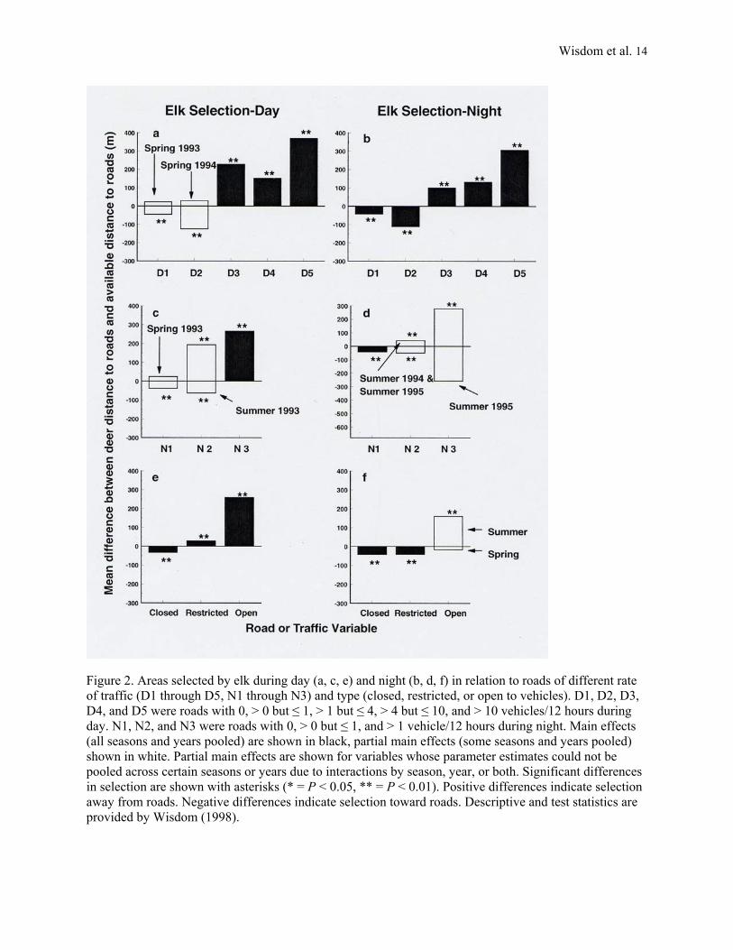
Both day and night, elk selected areas farther from roads that had day rates of >1 vehicles/12 hours (D3, D4, and D5, Figure 2a, b). Elk also selected areas farther from roads that had night rates of >1 vehicle/12 hours (N3, Figure 2c, d) and farther from roads open to motorized traffic (Open, Figure 2e, f). During night, summer 1995, however, elk showed no selection in relation to roads having night rates of >1 vehicles/12 hours (N3, Figure 2d). Elk also showed no selection during night in relation to open roads for spring, all years (Figure 2f).

The consistency of elk selection away from roads appeared to increase with increasing rate of traffic: roads with the highest rates--D3, D4, and D5--had no significant season or year interactions. Roads with the highest rate of traffic--D5--also had greatest mean difference between use and availability.

In contrast to typically selecting areas farther from open roads and farther from roads that had higher rates of traffic, elk generally selected areas closer to roads that had little or no traffic. However, the pattern was not consistent among all season-year periods. Specifically, elk were closer to roads that had day rates of >0 but ≤1 vehicles/12 hours (D2, Figure 2a, c, except for spring 1994 during day), closer to roads with no traffic (D1, Figure 2a, b, except for spring 1993; and N1, Figure 2c, d, except for spring 1993) and closer to roads that were closed (Closed, Figure 2e, f). However, elk showed either an opposite or an inconsistent pattern of selection, day versus night, in relation to roads that had night rates of >0 but ≤1 vehicles/12 hours (N2, Figure 2c, d). During day, elk also selected areas farther from roads restricted to administrative traffic (Restricted, Figure 2e) but selected areas closer to these same roads during night (Restricted, Figure 2f).

Between-species Selection: Deer versus Elk

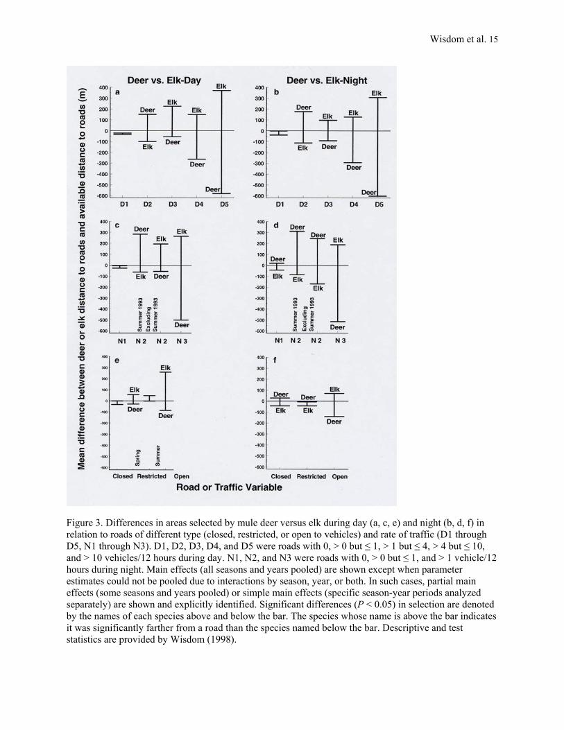
Both day and night, elk were farther than deer from roads that had traffic rates of >1 vehicles/12 hours (D3, N3, D4, and D5, Figure 3a, b, c, d) and farther than deer from open roads (Open, Figure 3e, f). By contrast, deer generally were farther than elk from roads that had lower traffic rates or that were restricted or closed, especially during night. Specifically, deer were farther than elk from roads having

Wisdom et al. 6

day rates of >0 but ≤1 vehicles/12 hours (D2, Figure 3a, b), farther than elk during night from roads having night rates of >0 but ≤1 vehicles/12 hours (N2, Figure 3d, except for summer 1993), and farther than elk during night from roads that were restricted or closed (Restricted, Closed, Figure 3f). During day, however, deer were closer than elk to N2 roads (Figure 3c, except for summer 1993) and closer than elk to restricted roads during spring, all years (Restricted, Figure 3e). Finally, we found no difference in deer versus elk selection in relation to roads with zero traffic (D1, N1, Figure 3a-d), except during night, when deer were farther than elk (N1, Figure 3d). We also found no difference in deer versus elk selection during day in relation to closed roads (Closed, Figure 3e).

Discussion

Selection Patterns

A number of strong and surprising patterns emerged from our results. First, deer and elk selected areas in opposite ways in relation to rate of traffic, with the magnitude of difference increasing with increasing rate of traffic. Second, thresholds existed for both species in terms of direction in selection: elk were generally farther from roads with traffic rates >1 vehicles/12 hours, both day and night, while deer were closer; by contrast, selection by both species was inconsistent in relation to roads with little or no traffic (≤1 vehicles/12 hours). Third, the type of road often correctly indexed the direction in selection shown by both species in relation to rates of traffic; that is, elk were farther from and deer were closer to roads that were open to all vehicular travel, which agreed with the overall direction in selection shown by both species in relation to most roads that had non-zero rates of traffic (i.e., all roads having >1 vehicles/12 hours). Moreover, both species showed a weak or inconsistent pattern of selection in relation to closed or restricted roads, which agreed with the inconsistent pattern of selection shown by both species in relation to roads with little or no traffic (≤1 vehicles/12 hours). And fourth, the type of road sometimes failed to index the magnitude of selection in relation to the traffic variables. For example, mule deer were approximately 100-150 yards (91-137 m) closer to open roads than available, yet deer were more than 250 yards (229 m) farther from roads of second-highest traffic rate (D4), and more than 550 yards (505 m) farther from roads of highest traffic rate (D5).

Implications for Roads and Habitat Models

Our results have direct bearing on a number of key assumptions and relationships contained in habitat models for elk. First, our results support the inclusion of an open roads variable in spring-summer habitat models, such as done in models by Thomas et al. (1979), Leege (1984), Lyon et al. (1985), Wisdom et al. (1986), and Johnson et al. (1996). Second, our results corroborate the assumption by some elk habitat modelers (e.g., Thomas et al. 1979, Wisdom et al. 1986) that increasing rate of traffic exerts an increasingly strong effect on elk selection; this implies that accuracy of elk habitat models could be improved by substituting a variable on traffic rate for the currently-used variable on open roads. Third, our findings do not support the assumption (Thomas et al. 1979) that selection by mule deer is similar to that by elk in relation to traffic and road variables; instead, our findings suggest that separate modeling terms are needed for each species. And fourth, our results call into question the use of carrying capacity models that are strictly nutrition- or forage-based, such as those by Nelson (1984), Cooperrider and Bailey (1984), Van Dyne et al. (1984), and Schwartz and Hobbs (1985), due to the strong effect that traffic and traffic-indexed human activities may have on modeling results. In contrast to these models, our findings provide compelling justification for the inclusion of traffic variables as a potential decrement to any projections of carrying capacity for both species.

Our results would be particularly useful when considered as part of “distance band” assessment of roads, as recently proposed by Rowland et al. (2004). Under such an assessment, all roads open to traffic are mapped, and the associated landscape is subdivided into distance intervals or bands, according to the distance of each band to the nearest open road. The probability that elk will use each distance band, based

Wisdom et al. 7

on prior research on elk distributions in relation to distance from open roads (Rowland et al. 2000), is then assigned to each band. These probabilities are then weighted by the area of each distance band occurring on the landscape being evaluated, and an overall probability calculated. If open roads could be further characterized by traffic rates, that probabilities of elk use by distance to nearest road of each rate could be considered. This refinement in the road-distance band assessment deserves further consideration in future modeling of elk habitat use at landscape scales such as watersheds.

Are Elk Displacing Deer?

Perhaps our most intriguing finding relates to the hypothesis of interference or disturbance competition, where “the mere presence of an animal intimidates or annoys another animal into leaving the area” (Nelson 1982:416). In the past, this hypothesis has been tested in relation to potential displacement of wild ungulates by domestic livestock. For example, many studies have shown that elk avoid or decrease their use of areas with the onset of cattle grazing (Knowles and Campbell 1982, Lonner and Mackie 1983, Wallace and Krausman 1987, Frisina 1992, Yeo et al. 1993, Coe et al. 2001, 2004), suggesting that interference competition may be operating.

The interference competition hypothesis, however, has not been tested rigorously between sympatric species of wild ungulates in North America. In potential support of this hypothesis in relation to mule deer and elk, a number of researchers (Cliff 1939, Mackie 1981, Nelson 1982) inferred that elk may out-compete and potentially displace mule deer on winter ranges that are limited in size and available forage. Nelson (1982) also believed that mule deer may leave or avoid areas of heavy use by elk, even if forage is abundant and dietary overlap with elk is low. Wisdom and Thomas (1996) also suggested that elk may displace mule deer on jointly occupied ranges when elk exist at moderate to high densities, due to a number of behavioral and physiological advantages that elk presumably have over deer. Finally, Cowan (1950:582), working in western Canada, inferred that “mule deer and moose have decreased since elk became abundant, and the causal nature of the two events, though not established, seems probable.”

Lack of direct, cause-effect evidence, however, limits firm conclusions. On the other hand, an additional analysis at Starkey (M. J. Wisdom, unpublished data) supports the assumption that mule deer change their distributions within our study area in relation to opposite changes in distribution by elk. In this additional analysis, elk were significantly farther (P < 0.05) from roads that had highest rate of traffic (D5) during summer 1994 (use minus availability = 338 yards), while mule deer were closer (use minus availability = - 412 yards). During a one-month, either-sex bow season on elk that immediately followed summer 1994, however, elk shifted their distributions significantly closer to these same roads (use minus availability = - 227 yards) while deer moved significantly farther away (use minus availability = 388 yards). Simultaneous with the shift by elk toward the D5 roads during the bow-hunt was the inclusion of the D5 roads within a no-hunting area that extended 400 yards outward from these roads. Thus, the most plausible, logical explanation for these distributional shifts is that elk are sensitive to traffic but more sensitive to hunting pressure; and that mule deer are sensitive to the presence of elk. The results, we believe, are distributions of mule deer and elk that exist and shift in dynamic, opposite ways, both in direction and magnitude, in agreement with the interference competition hypothesis.

Similar findings and inferences were made from earlier analyses of mule deer and elk interactions at Starkey by Johnson et al. (2000), Coe et al. (2001, 2004), and Stewart et al. (2002). In each of these analyses, investigators found strong evidence, although observational, that mule deer were avoiding elk. For example, Johnson et al. (2000) found that the strongest coefficient in explaining resource selection by mule deer was resource selection by elk. While mule deer occupied areas largely avoided by elk, the opposite was not true. That is, resource selection by elk could not be explained by selection patterns of mule deer.

Although such discussion is compelling, manipulative experiments are needed to formally test and validate the interference competition hypothesis under varying levels of deer and elk densities and rates of traffic, under the presumption that certain ungulate densities and certain traffic rates work together to cause elk to avoid areas near roads, and to cause mule deer to select areas near roads as a

Wisdom et al. 8

means of avoiding elk. Ideally, such manipulative experiments should be designed to measure effects on population performance of both species. To date, analyses of the effect of vehicle access on survival (such as Unwsorth et al. 1993 and Cole et al. 1998 for elk) and reproduction of both species on jointly occupied range has not been conducted.

It also is important to note that some researchers have speculated that mule deer are attracted to areas near roads when roadsides have been seeded with nutritious grasses and forbs (Wallmo et al. 1976). However, attraction to forage along roadsides would not plausibly account for the large differences in mule deer selection that we observed in relation to varying rates of traffic. Moreover, the distributional shifts described above for mule deer versus elk before versus during the 1994 bow-hunt provide compelling support for the interference competition hypothesis, which does not accommodate the notion that mule deer selected areas near roads due to superior roadside forage.

Limits of Inference Our findings particularly are relevant to spring and summer ranges that are jointly occupied by deer and elk under conditions of moderate to high densities of elk. These are the conditions under which our study was conducted. However, these conditions are common across large areas of western North America. By contrast, inferring results from our study to other areas where mule deer are common and elk are absent or sparse, would be inappropriate and likely unreliable. Inferring results of our study to spring and summer ranges occupied solely by mule deer, in particular, could be especially unreliable, given the high potential for mule deer distributions in our study area to be affected strongly by selection patterns of elk. In the absence of moderate or high densities of elk, mule deer may exhibit different distribution and selection patterns in relation to roads and traffic than we observed at Starkey. Management Implications

Differences in selection by mule deer and elk in relation to traffic could be considered in the management of motorized vehicles and traffic-related human activities on spring-summer ranges where both species occur, and where elk exist at moderate to high densities. Our results suggest that spring-summer habitat models for elk may not account for patterns of resource selection by mule deer on jointly occupied range, and that resource needs of each species must be addressed separately.

Our results also suggest that inclusion of road or traffic variables in habitat models is essential to accurate portrayal of selection patterns for both species. Forage- or nutrition-based habitat models that exclude road or traffic variables have the potential to be highly inaccurate, given the large magnitude of difference in selection shown by sympatric populations of deer and elk in relation to rates of traffic and types of roads. Manipulative experiments are needed to validate the presumption that rate of traffic acts as a mechanistic cause for differences in selection patterns between mule deer and elk, and to validate these selection patterns across a diversity of environments in which both species occur.

Acknowledgments

We are indebted to A. Ager, C. Borum, P. Coe, R. Collins, B. Dick, L. Erickson, R. Kennedy, S. Findholt, J. Nothwang, J. Noyes, D. Leckenby, R. Stussy, B.Wales and the many other current or former Starkey personnel who provided needed support for collection or management of data used in the analysis. We thank R. Steinhorst for statistical guidance and J. Peek, R. Steinhorst, and M. Rowland for their reviews of our paper. Logistical support was provided by L. Norris, R. Pedersen, H. Black, Jr., R. Devlin, and R. Escano. Financial support was provided by U.S. Department of Agriculture Forest Service, Pacific Northwest Region, Oregon Department of Fish and Wildlife, and U.S. Department of Agriculture Forest Service, Pacific Northwest Research Station.

Wisdom et al. 9

Literature Cited Ager, A. A., and R. J. McGaughey. 1997. UTOOLS: microcomputer software spatial analysis and

landscape visualization. U.S. Department of Agriculture Forest Service, Pacific Northwest Research Station General Technical Report, PNW-GTR-397, Portland, Oregon.

Ager, A. A., B. K. Johnson, P. K. Coe, and M. J. Wisdom. 2004. Landscape simulation of foraging by elk, mule deer, and cattle on summer range. Transactions of the North American Wildlife and Natural Resources Conference 69: in press.

Cliff, E. P. 1939. Relationships between elk and mule deer in the Blue Mountains of Oregon. Transactions of the North American Wildlife and Natural Resources Conference 4:560-569.

Coe, P. K., B. K. Johnson, J. W. Kern, S. L. Findholt, J. G. Kie, and M. J. Wisdom. 2001. Responses of elk and mule deer to cattle in summer. Journal of Range Management 54:205, A51-A76.

Coe, P. K., B. K. Johnson, K. M. Stewart, and J. G. Kie. 2004. Spatial and temporal interactions of elk, mule deer, and cattle. Transactions of the North American Wildlife and Natural Resources Conference 69: in press.

Cole, E. K., M. D. Pope, and R. G. Anthony. 1998. Effects of road management on movement and survival of Roosevelt elk. Journal of Wildlife Management 61:1115-1126.

Cooperrider, A. Y., and J. A. Bailey. 1984. A simulation approach to forage allocation. In Developing strategies for rangeland management, 525-560. Westview Press, Boulder, Colorado, USA.

Cowan, I. M. 1950. Some vital statistics of big game on over-stocked mountain range. Transactions of the North American Wildlife and Natural Resources Conference 15:581-589.

Findholt, S. L., B. K. Johnson, L. D. Bryant, and J. W. Thomas. 1996. Corrections for position bias of a LORAN-C radio-telemetry system using DGPS. Northwest Science 70:273-280.

Frisina, M. R. 1992. Elk habitat use within a rest-rotation grazing system. Rangelands 14:93-96. Johnson, B. K., A. Ager, S. A. Crim, M. Wisdom, S. L. Findholt, and D. Sheehy. 1996. Allocating forage

among wild and domestic ungulates--a new approach. 166-169 eds. Proceedings, Sustaining rangeland ecosystems symposium, SR 953, eds. W. D. Edge and S. L. Olson-Edge, 166-169. Corvallis: Oregon State University.

Johnson, B. K., A. A. Ager, S. L. Findholt, M. J. Wisdom, D. B. Marx, J. W. Kern, and L. D. Bryant. 1998. Mitigating spatial differences in observation rate of automated telemetry systems. Journal of Wildlife Management 62:958-967.

Johnson, B. K, J. W. Kern, M. J. Wisdom, S. L. Findholt, and J. G. Kie. 2000. Resource selection and spatial separation of mule deer and elk in spring. Journal of Wildlife Management 64:685-697.

Kirk, R. E. 1982. Experimental design: procedures for the behavioral sciences. Second edition, Pacific Grove, California: Brooks/Cole Publishing Company.

Knowles, C. J., and R. B. Campbell. 1982. Distribution of elk and cattle in a rest-rotation grazing system. In Wildlife-livestock relationships symposium: proceedings 10, eds. J. M. Peek and P. D. Dalke, 46-60. Moscow: Wildlife and Range Experiment Station, University of Idaho.

Leege, T. A. 1984. Guidelines for evaluating and managing summer elk habitat in northern Idaho. Idaho Department of Fish and Game, Wildlife Bulletin Number 11, Boise.

Lonner, T. N., and R. J. Mackie. 1983. On the nature of competition between big game and livestock. In Proceedings Forestland grazing symposium, eds. B. F. Roche, Jr., and D. M. Baumgartner, 53-58. Pullman: Washington State University.

Lyon, L. J. 1983. Road density models describing habitat effectiveness for elk. Journal of Forestry 81:592-595.

Lyon, L. J., T. N. Lonner, J. P. Weigand, C. L. Marcum, W. D. Edge, J. D. Jones, D. W. McCleerey, and L. L. Hicks. 1985. Coordinating elk and timber management, final report of the Montana cooperative elk-logging study, 1970-1985. Helena: Montana Department of Fish, Wildlife, and Parks.

Wisdom et al. 10

Lyon, L.J., and A.G. Christensen. 2002. Elk and land management. In North American elk, ecology and management, eds. D.E. Toweill and J.W. Thomas, 557-581. Washington, DC: Smithsonian Institution Press.

Mackie, R. J. 1981. Interspecific relationships. In Mule and black-tailed deer of North America, ed. O. C. Wallmo, 487-507. Lincoln: University of Nebraska Press.

Nelson, J. R. 1982. Relationships of elk and other large herbivores. In Elk of North America, ecology and management, eds. J. W. Thomas and D. E. Toweill, 415-441. Harrisburg, Pennsylvania: Stackpole Books.

Nelson, J. R. 1984. A modeling approach to large herbivore competition. In Developing strategies for rangeland management, 491-524. Boulder, Colorado: Westview Press.

Perry, C., and R. Overly. 1977. Impact of roads on big game distributions in portions of the Blue Mountains of Washington, 1972-1973. Applied Research Bulletin Number 11, Washington Department of Game, Olympia, Washington.

Rost, G. R., and J. A. Bailey. 1979. Distribution of mule deer and elk in relation to roads. Journal of Wildlife Management 43:634-641.

Rowland, M. M., L. D. Bryant, Bruce K. Johnson, J. H. Noyes, M. J. Wisdom, and J. W. Thomas. 1997. The Starkey Project: history, facilities, and data collection methods for ungulate research. U.S. Department of Agriculture Forest Service, Pacific Northwest Research Station General Technical Report, PNW-GTR-396, Portland, Oregon.

Rowland, M. M., P. Coe, R. Stussy, B. K. Johnson, M. J. Wisdom, and N. J. Cimon. 1998. The Starkey habitat database for ungulate research: construction, documentation, and use. U.S. Department of Agriculture Forest Service, Pacific Northwest Research Station General Technical Report, PNW-GTR-430, Portland, Oregon.

Rowland, M. M., M. J. Wisdom, B. K. Johnson, and J. G. Kie. 2000. Elk distribution and modeling in relation to roads. Journal of Wildlife Management 64:672-684.

Rowland, M. M., M. J. Wisdom, B. K. Johnson, and M. A. Penninger. 2004. Effects of roads on elk: Implications for management in forested ecosystems. Transactions of the North American Wildlife and Natural Resources Conference 69: in press.

SAS Inst., Inc. 1990. SAS/STAT User’s Guide, volumes 1 and 2. Cary, North Carolina: SAS Institute, Incorporated.

Schwartz, C. C., and N. T. Hobbs. 1985. Forage and range evaluation. In Bioenergetics of wild herbivores, eds. R. J. Hudson and R. G. White, 26-51. Boca Raton, Florida: CRC Press.

Stewart, K. M., R. T. Bowyer, J. G. Kie, N. J. Cimon, and B. K. Johnson. 2002. Temporospatial distributions of elk, mule deer, and cattle: Resource partitioning and competitive displacement. Journal of Mammalogy 83:229-244.

Thomas, J. W. H. Black, R. J. Scherzinger, and R. J. Pedersen. 1979. Deer and elk. In Wildlife habitats in managed forests--the Blue Mountains of Oregon and Washington, ed. J. W. Thomas, 104-127. U.S. Department of Agriculture Forest Service, Agricultural Handbook Number 553, Washington, D.C.

Thomas, J. W., D. A. Leckenby, M. Henjum, R. J. Pedersen, and L. D. Bryant. 1988. Habitat effectiveness index for elk on Blue Mountain winter ranges. U.S. Department of Agriculture Forest Service, Pacific Northwest Research Station General Technical Report, PNW-GTR-218, Portland, Oregon.

Van Dyne, G. M., P. T. Kortopates, and F. M. Smith. 1984. Quantitative frameworks for forage allocation. In Developing strategies for rangeland management, 289-412. Boulder, Colorado: Westview Press.

Wallace, M. C., and P. R. Krausman. 1987. Elk, mule deer, and cattle habitats in central Arizona. Journal of Range Management 40:80-83.

Wallmo, O. C., D. F. Reed, and L. H. Carpenter. 1976. Alteration of mule deer habitat by wildfire, logging, highways, agriculture, and housing developments. In Proceedings, mule deer decline in the West, a symposium, eds. G. W. Workman and J. B. Low, 37-47. Logan: Utah State University.

Wisdom et al. 11

Wisdom, M. J. 1998. Assessing life-stage importance and resource selection for conservation of selected vertebrates. Ph.D. dissertation, University of Idaho, Moscow.

Wisdom, M. J., L. R. Bright, C. G. Carey, W. W. Hines, R. J. Pedersen, D. A. Smithey, J. W. Thomas, and G. W. Witmer. 1986. A model to evaluate elk habitat in western Oregon. U.S. Department of Agriculture Forest Service Publication No. R6-F&WL-216-1986, Portland, Oregon.

Wisdom, M. J., and J. W. Thomas. 1996. Elk. In Rangeland wildlife, ed. P.R. Krausman, 157-181. Denver, Colorado: Society For Range Management.

Wisdom, M. J., M. M. Rowland, B. K. Johnson, and B. Dick. 2004. Overview of the Starkey Project: Mule deer and elk research for management benefits. Transactions of the North American Wildlife and Natural Resources Conference 69: in press.

Witmer, G. W., and D. S. deCalesta. 1985. Effect of forest roads on habitat use by Roosevelt elk. Northwest Science 59:122-125.

Yeo, J. F., J. M. Peek, W. T. Wittinger, and C. T. Kvale. 1993. Influence of rest-rotation cattle grazing on mule deer and elk habitat use in east-central Idaho. Journal of Range Management 46:245-250.

Wisdom et al. 12

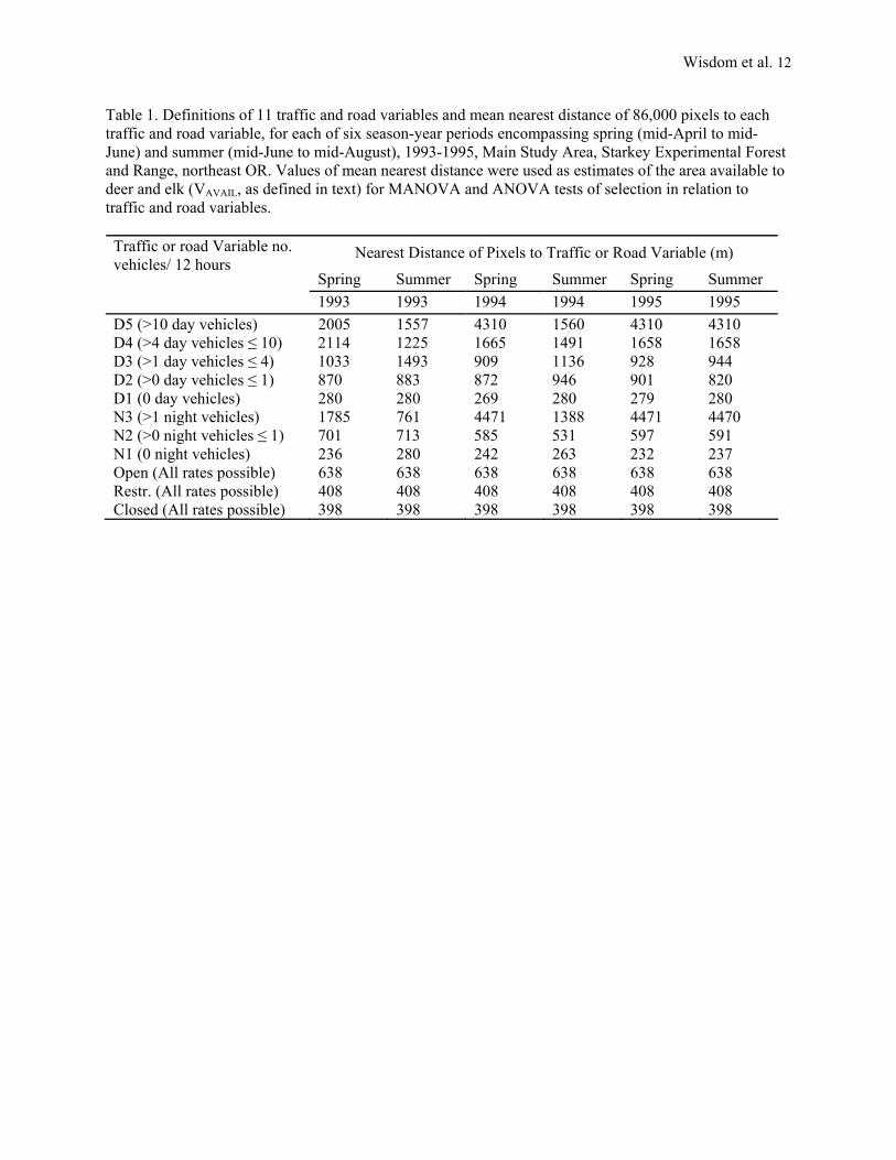
Table 1. Definitions of 11 traffic and road variables and mean nearest distance of 86,000 pixels to each traffic and road variable, for each of six season-year periods encompassing spring (mid-April to mid-June) and summer (mid-June to mid-August), 1993-1995, Main Study Area, Starkey Experimental Forest and Range, northeast OR. Values of mean nearest distance were used as estimates of the area available to deer and elk (VAVAIL, as defined in text) for MANOVA and ANOVA tests of selection in relation to traffic and road variables.

Nearest Distance of Pixels to Traffic or Road Variable (m)

Spring Summer Spring Summer Spring Summer

Traffic or road Variable no. vehicles/ 12 hours

1993 1993 1994 1994 1995 1995 D5 (>10 day vehicles) 2005 1557 4310 1560 4310 4310 D4 (>4 day vehicles ≤ 10) 2114 1225 1665 1491 1658 1658 D3 (>1 day vehicles ≤ 4) 1033 1493 909 1136 928 944 D2 (>0 day vehicles ≤ 1) 870 883 872 946 901 820 D1 (0 day vehicles) 280 280 269 280 279 280 N3 (>1 night vehicles) 1785 761 4471 1388 4471 4470 N2 (>0 night vehicles ≤ 1) 701 713 585 531 597 591 N1 (0 night vehicles) 236 280 242 263 232 237 Open (All rates possible) 638 638 638 638 638 638 Restr. (All rates possible) 408 408 408 408 408 408 Closed (All rates possible) 398 398 398 398 398 398

Wisdom et al. 13

Figure 1. Areas selected by mule deer during day (a, c, e) and night (b, d, f) in relation to roads of different rate of traffic (D1 through D5, N1 through N3) and type (closed, restricted, or open to vehicles). D1, D2, D3, D4, and D5 were roads with 0, > 0 but ≤ 1, > 1 but ≤ 4, > 4 but ≤ 10, and > 10 vehicles/12 hours during day. N1, N2, and N3 were roads with 0, > 0 but ≤ 1, and > 1 vehicle/12 hours during night. Main effects (all seasons and years pooled) are shown in black and partial main effects (some seasons and years pooled) shown in white. Partial main effects are shown for variables whose parameter estimates could not be pooled across certain seasons or years due to interactions by season, year, or both. Significant differences in selection are shown with asterisks ( * = P < 0.05, ** = P < 0.01). Positive differences indicate selection away from roads. Negative differences indicate selection toward roads. Descriptive and test statistics are provided by Wisdom (1998).

Wisdom et al. 14

Figure 2. Areas selected by elk during day (a, c, e) and night (b, d, f) in relation to roads of different rate of traffic (D1 through D5, N1 through N3) and type (closed, restricted, or open to vehicles). D1, D2, D3, D4, and D5 were roads with 0, > 0 but ≤ 1, > 1 but ≤ 4, > 4 but ≤ 10, and > 10 vehicles/12 hours during day. N1, N2, and N3 were roads with 0, > 0 but ≤ 1, and > 1 vehicle/12 hours during night. Main effects (all seasons and years pooled) are shown in black, partial main effects (some seasons and years pooled) shown in white. Partial main effects are shown for variables whose parameter estimates could not be pooled across certain seasons or years due to interactions by season, year, or both. Significant differences in selection are shown with asterisks (* = P < 0.05, ** = P < 0.01). Positive differences indicate selection away from roads. Negative differences indicate selection toward roads. Descriptive and test statistics are provided by Wisdom (1998).

Wisdom et al. 15

Figure 3. Differences in areas selected by mule deer versus elk during day (a, c, e) and night (b, d, f) in relation to roads of different type (closed, restricted, or open to vehicles) and rate of traffic (D1 through D5, N1 through N3). D1, D2, D3, D4, and D5 were roads with 0, > 0 but ≤ 1, > 1 but ≤ 4, > 4 but ≤ 10, and > 10 vehicles/12 hours during day. N1, N2, and N3 were roads with 0, > 0 but ≤ 1, and > 1 vehicle/12 hours during night. Main effects (all seasons and years pooled) are shown except when parameter estimates could not be pooled due to interactions by season, year, or both. In such cases, partial main effects (some seasons and years pooled) or simple main effects (specific season-year periods analyzed separately) are shown and explicitly identified. Significant differences (P < 0.05) in selection are denoted by the names of each species above and below the bar. The species whose name is above the bar indicates it was significantly farther from a road than the species named below the bar. Descriptive and test statistics are provided by Wisdom (1998).