spatial modeling of agricultural land use change at global scale
TRANSCRIPT
S
Pa
b
c
a
ARRA
KPDISVL
1
bat2ttcSb
i
(
h0
Ecological Modelling 291 (2014) 152–174
Contents lists available at ScienceDirect
Ecological Modelling
j ourna l h omepa ge: www.elsev ier .com/ locate /eco lmodel
patial modeling of agricultural land use change at global scale
rasanth Meiyappana,∗, Michael Daltonb, Brian C. O’Neill c, Atul K. Jaina,∗∗
Department of Atmospheric Sciences, University of Illinois, Urbana, IL 61801, USAAlaska Fisheries Science Center, National Ocean and Atmospheric Administration, National Marine Fisheries Service, Seattle, WA 98115, USAClimate and Global Dynamics Division, National Center for Atmospheric Research, Boulder, CO 80307, USA
r t i c l e i n f o
rticle history:eceived 28 April 2014eceived in revised form 23 July 2014ccepted 25 July 2014
eywords:redictionrivers
ntegrated Assessmentpatially explicitalidationand change
a b s t r a c t
Long-term modeling of agricultural land use is central in global scale assessments of climate change, foodsecurity, biodiversity, and climate adaptation and mitigation policies. We present a global-scale dynamicland use allocation model and show that it can reproduce the broad spatial features of the past 100years of evolution of cropland and pastureland patterns. The modeling approach integrates economictheory, observed land use history, and data on both socioeconomic and biophysical determinants ofland use change, and estimates relationships using long-term historical data, thereby making it suitablefor long-term projections. The underlying economic motivation is maximization of expected profits byhypothesized landowners within each grid cell. The model predicts fractional land use for cropland andpastureland within each grid cell based on socioeconomic and biophysical driving factors that changewith time. The model explicitly incorporates the following key features: (1) land use competition, (2)spatial heterogeneity in the nature of driving factors across geographic regions, (3) spatial heterogeneityin the relative importance of driving factors and previous land use patterns in determining land useallocation, and (4) spatial and temporal autocorrelation in land use patterns.
We show that land use allocation approaches based solely on previous land use history (but disre-garding the impact of driving factors), or those accounting for both land use history and driving factors
by mechanistically fitting models for the spatial processes of land use change do not reproduce welllong-term historical land use patterns. With an example application to the terrestrial carbon cycle, weshow that such inaccuracies in land use allocation can translate into significant implications for globalenvironmental assessments. The modeling approach and its evaluation provide an example that can beuseful to the land use, Integrated Assessment, and the Earth system modeling communities.© 2014 The Authors. Published by Elsevier B.V. This is an open access article under the CC BY-NC-ND
. Introduction
Changes in land use are driven by non-linear interactionsetween socioeconomic conditions (e.g. population, technology,nd economy), biophysical characteristics of the land (e.g. soil,opography, and climate), and land use history (Lambin et al., 2001,003). The spatial heterogeneity in driving factors has led to spa-
ially distinct land use patterns. Land use change models exploitechniques to understand the spatial relationship between histori-al changes in land use and its driving factors (or proxies for them).uch models are also used to project spatial changes in land useased on scenarios of changes in its drivers. The importance of∗ Corresponding author at: 105 South Gregory Street, Atmospheric Sciences Build-ng, Urbana, IL 61801, USA. Tel.: +1 217 898 1947.∗∗ Corresponding author. Tel.: +1 217 333 2128.
E-mail addresses: [email protected], [email protected]. Meiyappan), [email protected] (A.K. Jain).
ttp://dx.doi.org/10.1016/j.ecolmodel.2014.07.027304-3800/© 2014 The Authors. Published by Elsevier B.V. This is an open access article un
license (http://creativecommons.org/licenses/by-nc-nd/3.0/).
land use change models is evident from the wide range of exist-ing modeling approaches and applications (see reviews by NRC,2014; Heistermann et al., 2006; Verburg et al., 2004; Parker et al.,2003; Agarwal et al., 2002; Irwin and Geoghegan, 2001; Briassoulis,2000; U.S. EPA, 2000). However, most land use change models aredesigned for local to regional scale studies (typically sub-nationalto national level); global-scale modeling approaches are scarce(Rounsevell and Arneth, 2011; Heistermann et al., 2006).
Global-scale land use modeling is challenging compared tosmaller-scale approaches for three main reasons. First, the set ofdriving factors and their spatial characteristics of change are diverseacross the globe, and models need to represent this variability (vanAsselen and Verburg, 2012). Second, the various factors that affectland use decisions operate at different spatial scales. For example,
landowners make decisions at local scale, whereas factors like gov-ernance, institutions, and enforcement of property rights operate atmuch larger scales. Ideally, global-scale models should incorporatethe effects of driving factors at multiple scales (Rounsevell et al.,der the CC BY-NC-ND license (http://creativecommons.org/licenses/by-nc-nd/3.0/).
al Mo
2scTdg2
lctesSmlist(w2a
Iacmesmdahlridvaee(G22
sllmeed
cndmcGta2el
P. Meiyappan et al. / Ecologic
014; Heistermann et al., 2006). However, an integrated under-tanding of how the multi-scale drivers combine to cause land usehange is far from complete (Lambin et al., 2001; Meyfroidt, 2013).hird, spatially and temporally consistent data for many importantriving factors (e.g. market influence) are not readily available at alobal scale and at the required spatial resolution (Verburg et al.,011, 2013).
Despite these challenges, there are three reasons for modelingand use at a global scale. First, several key drivers of land use (e.g.limate) and their impacts on land use have no regional demarca-ions and substantial feedback exists between them (Rounsevellt al., 2014). Addressing the feedback between land use andocioecological systems requires a globally consistent framework.econd, regions across the world are interconnected through globalarkets and trade that can shift supply responses to demands for
and across geopolitical regions (Meyfroidt et al., 2013). Model-ng such complex interactions among economies demands a globalcale approach. Third, the aggregate consequences of land use athe global scale have significant consequences for climate changePielke et al., 2011), global biogeochemical cycles (Jain et al., 2013),ater resources (Bennett et al., 2001) and biodiversity (Phalan et al.,
011), making global land use modeling a useful component ofnalyses of these issues.
These reasons have motivated global scale assessments usingntegrated Assessment Models (IAMs) that seek to treat the inter-ctions between land and other socioecological systems in a fullyoupled manner (Sarofim and Reilly, 2011). In IAMs, socioeconomicodels are coupled with biophysical models (process-based veg-
tation models and/or climate models) to translate socioeconomiccenarios into changes in land cover and its impacts on environ-ental variables of interest (van Vuuren et al., 2012). IAMs typically
isaggregate the world into 14–24 regions (van Vuuren et al., 2011),nd land use decisions are made at this regional scale. Some IAMsave spatially explicit biophysical components, and in these cases
and use information on geographic grids at a much higher spatialesolution is required (typically 0.5◦ × 0.5◦ lat/long). To provide thisnformation, spatial land use allocation approaches are employed toownscale aggregate land demands for large world regions to indi-idual grid cells. Examples of such global scale land use allocationpproaches can be found in the Global Forest Model (Rokityanskiyt al., 2007), IMAGE (Bouwman et al., 2006), MagPie (Lotze-Campent al., 2010), KLUM (Ronneberger et al., 2005, 2009), MIT-IGSMReilly et al., 2012; Wang, 2008), GLOBIO3 (Alkemade et al., 2009),LOBIOM (Havlik et al., 2011), Nexus land use model (Souty et al.,012, 2013), and the Global Land use Model (GLM) (Hurtt et al.,011).
In this article, we develop a new global land use allocation modelpecifically to downscale agricultural (cropland and pastureland)and use from large world regions to the grid cell level. Agriculturaland use merits special attention because it is associated with the
ajority of land use-related environmental consequences (Greent al., 2005), currently occupying ∼40% of Earth’s land area (Foleyt al., 2005). There are two novel features of our approach thatistinguish it from previous approaches.
First, our model predicts fractional land use within each gridell (continuous field approach) driven by time-varying socioeco-omic and biophysical factors. In contrast, most existing modelso one or the other but not both. For example, many downscalingethods represent land use in each grid cell (0.5◦ × 0.5◦ lat/long or
oarser) by the dominant land cover category (e.g. MagPie, IMAGE,LOBIOM, and the Nexus land use model). This simplified represen-
ation in land cover underestimates land cover heterogeneity and is
major source of uncertainty in impact assessments (Verburg et al.,013). Some recent efforts (e.g. Letourneau et al., 2012; Schaldacht al., 2011) have addressed this problem by increasing spatial reso-ution, for example using 5-min grid cells that represent dominantdelling 291 (2014) 152–174 153
land cover types. While such approaches are an improvement, theyare also much more computationally intensive and do not escapethe problem that for many variables representing land use drivers,high resolution data at the global scale are unavailable (Verburget al., 2013). In other approaches (e.g., GLOBIO3 and GLM) landcover is represented as fractional units within each grid cell (again0.5◦ × 0.5◦ lat/long), but the approach to allocation is overly sim-plified, proportionally allocating land use projections for aggregateregions to grid cells as closely as possible to existing land use pat-terns. Such an approach does not account for the effect of changesover time in land use drivers, which can lead to land use projectionsthat are inconsistent with those drivers (as will be shown later).
Second, we carry out the first global scale evaluation of a spatialland use allocation model over a long historical period (>100 years),reproducing the broad spatial features of the long-term evolutionof agricultural land use patterns. Evaluation of global-scale spatialland use models is important because they are used to generatescenarios for 50–100 years into the future, for example, to exploreissues related to greenhouse gas emissions and mitigation possi-bilities (Moss et al., 2010; Kindermann et al., 2008), climate changeimpacts on ecosystems (MEA, 2005; UNEP, 2012), biodiversity(TEEB, 2010; Pereira et al., 2010), or adaptation options involv-ing land use (OECD, 2012; Phalan et al., 2011). While evaluationof model performance over the past 100 years is no guarantee ofgood performance over the next 100 years, demonstrating the abil-ity of a model to reproduce long-term historical patterns increasesconfidence in its suitability for application to long-term scenariosof future change. The model evaluation presented here could serveas an example for how evaluation of other downscaling method-ologies could be carried out (O’Neill and Verburg, 2012; Hibbardet al., 2010).
2. Methods and data
2.1. Overview of the approach
Our land use allocation model simulates the spatial and tempo-ral development of cropland and pastureland at a spatial resolutionof 0.5◦ × 0.5◦ lat/long and at an annual time-step. The model opera-tes at two different spatial levels. On the regional level, theaggregate regional demand for cropland and pastureland is pro-vided as input to the model. The model then allocates this demandto individual grid cells within that region. We use a constrainedoptimization technique to allocate a fraction of each grid cell tocropland and pastureland while meeting the aggregate regionaldemand for each type of land. The optimization technique selectsthe most profitable land to grow crops and pasture based on (1)the suitability of each grid cell for crop or pasture production,determined by a set of 46 biophysical and socioeconomic factors(Table 1), (2) historical land use patterns (temporal autocorrelation)and (3) the land use predicted for neighboring grid cells (spatialautocorrelation).
A primary intended application of this model is as one com-ponent of a larger modeling framework that includes a global,regionally resolved economic model that generates scenarios offuture demand for land at the regional level, similar to the approachtaken in other IAMs or land use models as discussed above. How-ever, the main aim of this paper is to present and evaluate ourmodel in a historical simulation against 20th century gridded dataof cropland and pastureland. Ideally, the model should be evaluatedagainst observational data. However, purely observational data for
global, spatially resolved land use data do not exist. Rather, exist-ing gridded land use reconstructions are modeled estimates thatdraw on national and sub-national data to the extent possible (seeAppendix A). For practical purposes, we assume existing land use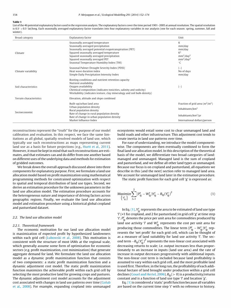
154 P. Meiyappan et al. / Ecological Modelling 291 (2014) 152–174
Table 1List of the 46 potential explanatory factors used in the regression analysis. The explanatory factors cover the time period 1901–2005 at annual resolution. The spatial resolutionis 0.5◦ × 0.5◦ lat/long. Each seasonally averaged explanatory factor translates into four explanatory variables in our analysis (one for each season: spring, summer, fall andwinter).
Broad category Explanatory factor Unit
Climate
Seasonally averaged temperature KSeasonally averaged precipitation mm/daySeasonally averaged potential evapotranspiration (PET) mm/daySquared seasonally averaged temperature K2
Squared seasonally averaged precipitation mm2/day2
Squared seasonally averaged PET mm2/day2
Seasonal Temperature Humidity Index (THI) ◦C
Climate variabilitySeasonal Palmer Drought Severity Index (PDSI) (–)Heat wave duration index No of daysSimple Daily Precipitation Intensity Index mm/day
Soil characteristics
Rooting conditions and nutrient retention capacity
(–)Nutrient availabilityOxygen availabilityChemical composition (indicates toxicities, salinity and sodicity)Workability (indicates texture, clay mineralogy and soil bulk-density)
Terrain characteristics Elevation, altitude and slope combined
Socioeconomic
Built-up/urban land area Fraction of grid area (m2/m2)Urban population density
Inhabitants/km2Rural population density
densit densi
rcitlHmoo
captdltgma
2
2
iwcwsamodfsTce
Rate of change in rural population
Rate of change in urban populationMarket Influence Index
econstructions represent the “truth” for the purpose of our modelalibration and evaluation. In this respect, we face the same lim-tations as all global, spatially resolved models of land use, whichypically use such reconstructions as maps representing currentand use as a basis for future projections (e.g., Hurtt et al., 2011).owever, it must be kept in mind that such reconstructions are esti-ates, and that estimates can and do differ from one another based
n different uses of the underlying data and methods for estimationf gridded outcomes.
We break down the overall approach discussed above into threeomponents for explanatory purpose. First, we formulate a land usellocation model based on profit maximization using mathematicalrogramming methods for constrained optimization with respecto spatial and temporal distribution of land use types. Second, weerive an estimation procedure for the unknown parameters in the
and use allocation model. The estimation procedure accounts forhe heterogeneous nature and importance of driving factors acrosseographic regions. Finally, we evaluate the land use allocationodel and estimation procedure using a historical global cropland
nd pastureland dataset.
.2. The land use allocation model
.2.1. Theoretical frameworkThe economic motivation for our land use allocation model
s maximization of expected profit by hypothesized landownersithin each grid cell (Lubowski et al., 2008). This motivation is
onsistent with the structure of most IAMs at the regional scale,hich generally assume some form of optimization for economic
ectors (e.g. profit maximization, cost minimization) that generateggregate demand for land. We formulate the land use allocationodel as a dynamic profit maximization function that consists
f two components: a static profit maximization function and aynamic adjustment cost model. The static profit maximizationunction maximizes the achievable profit within each grid cell by
electing the most productive land for growing crops and pastures.he dynamic adjustment cost model accounts for the adjustmentost associated with changes in land use patterns over time (Golubt al., 2008). For example, expanding cropland into unmanagedyInhabitants/km2/yrtyInternational dollars/person
ecosystems would entail some cost to clear unmanaged land andbuild roads and other infrastructure. This adjustment cost tends tocreate inertia in land use patterns over time.
For ease of understanding, we introduce the model component-wise. The components are then eventually combined to form thefinal land use allocation model. In this description of the theoreticalbasis of the model, we differentiate two broad categories of land:managed and unmanaged. Managed land is the sum of croplandand pastureland, and we define all other land types as unmanaged.Because our focus is on cropland and pastureland, all equations wedescribe in this (and the next) section refer to managed land area.We account for unmanaged land later in the estimation procedure.
The static profit function for each grid cell ‘g’ is expressed as:
Maximize{Yt
lg
} 2∑l=1
(Ptlg − Wt
lg)Ytlg − Rlg(Yt
lg)2
(1)
In Eq. (1), Ytlg
represents the area to be estimated of land use type‘l’ (=1 for cropland, and 2 for pastureland) in grid cell ‘g’ at time step‘t’. Pt
lgdenotes the price per unit area for commodities produced by
land use activity ‘l’ and Wtlg
represents the cost per unit area for
producing those commodities. The linear term (Ptlg
− Wtlg
)Ytlg
rep-resents the ‘net profit’ for each grid cell, which can be thought ofas a measure of land suitability for land use activity ‘l’. The sec-ond term −Rlg(Yt
lg)2 represents the non-linear cost associated with
decreasing returns to scale; i.e. output increases less than propor-tionately to an increase in inputs (land use area) and the rate ofincrease in output decreases progressively with additional inputs.The non-linear cost term is included because land profitability isassumed to vary within each grid cell, and the most profitable landis used first. Therefore, in the long run, the profitability of each addi-tional hectare of land brought under production within a grid cell
declines (Gouel and Hertel, 2006). Rlg(> 0) is a productivity/returnsconstant and is a function of land use type ‘l’ and location ‘g’.Eq. (1) is considered a ‘static’ profit function because all variablesare based on the current time step ‘t’ with no reference to history.
al Mo
Ef
M
si
Y
∑
cs
c
M
cabscfabe2
t
M
eutp
cT(
M
a[sTaSi
D
P. Meiyappan et al. / Ecologic
q. (1) can be simplified as a quadratic function (see Appendix E.1or detailed steps):
aximize{Yt
lg
} 2∑l=1
(−Rlg)(Ytlg − dlgSt
lg)2
(2)
In Eq. (2), dlg = (1/2Rlg) is a constant for decreasing returns tocale and St
lg(suitability) equals the net price term Pt
lg− Wt
lg. Eq. (2)
s subject to two constraints:
tlg≥0 (3)
2
l=1
Ytlg ≤ GAg (4)
Eq. (3) avoids negative allocations. Eq. (4) implies the total ofropland and pastureland area allocated within each grid cell ‘g’hould not exceed the grid cell area GAg .
We formulate a dynamic adjustment cost model for each gridell ‘g’ as follows:
inimize{Yt
lg
} 2∑l=1
Qlg(Ytlg − Yt
lg)2
(5)
Eq. (5) is also constrained by Eqs. (3) and (4). Eq. (5) represents aonstrained least-squares optimization that tends to minimize thedjustment cost by minimizing the changes in land use allocationetween the current and a previous time step t(t < t). Criteria forelecting the value of t are explained in Section 2.5. Qlg(> 0) is aonstant that indicates the adjustment cost per unit area and is aunction of land use type ‘l’ and location ‘g’. In Eq. (5) we assumen exponent of 2 because: (1) our land use allocation method isased on quadratic programming, and (2) our model parameterstimation involves differentiating the quadratic program (Section.3), which results in linear equations that are convenient to solve.
We combine Eqs. (2) and (5), to write the overall objective func-ion as a minimization problem for each grid cell ‘g’:
inimize{Yt
lg
} 2∑l=1
⎡⎣Qlg
(Yt
lg
GAg−
Ytlg
GAg
)2
+ Rlg
(Yt
lg
GAg− dlg
Stlg
GAg
)2⎤⎦ (6)
For convenience we have divided Eq. (6) by a constant thatquals the square of grid cell area. The minimization problem isnaffected by this modification. Later, it will become evident thatreating variables as fractions instead of areas is convenient in thearameter estimation procedure.
Our aim is to allocate the aggregate land demand among the gridells within a given region such that the total profits are maximized.herefore, we stack the individual grid cell level optimizations (Eq.6)) over the aggregate region and write in matrix notation:
inimize{Yt }
(Yt − Yt
)′A(Yt − Yt) +
(Yt − DSt
)′(Yt − DSt) (7)
In Eq. (7), primes denote the matrix transpose operator. Yt is column vector of size ‘2N × 1’ with elements (Yt
lg/GAg), i.e. Yt =
Yt11/GA1 Yt
21/GA1 · · · Yt1N/GAN Yt
2N/GAN
]′, where ‘N’ repre-
ents the total number of grid cells within the aggregate region.herefore, elements in vector Yt are normalized by the grid cellrea and will therefore range from zero to one. Similarly Yt , d, andt are vectors of Yt
lg/GAg , dlg , and St
lg/GAg , respectively. The term D
s a diagonal matrix of size ‘2N × 2N’ given by
= d ∗ I2N×2N
delling 291 (2014) 152–174 155
where I is an identity matrix. The term A represents a constantdiagonal matrix.
A =
⎡⎢⎢⎢⎢⎢⎢⎢⎢⎢⎢⎣
Q11
R110 · · · · · · 0
0Q21
R21
. . .. . .
...
.... . .
. . .. . .
......
. . .. . . Q1N
R1N0
0 · · · · · · 0Q2N
R2N
⎤⎥⎥⎥⎥⎥⎥⎥⎥⎥⎥⎦
2N×2N
.
The matrix A can be usefully interpreted as representing thebalance between the importance of adjustment costs and of landsuitability in determining land allocation across grid cells. Eq. (7)can be regarded as a balance between a dynamic (time-seriesaspect) and a static (cross-sectional aspect) term. The dynamic termis implicitly minimizing adjustment costs by trying to keep landuse similar to the historical (already existing) land use patterns,whereas the static term selects the most suitable land to maximizethe net profit regardless of history. The balance between the staticand dynamic term is determined by the values of the matrix A. Inextreme cases, when Rlg is zero, no explicit account is taken of therelative suitability of land across grid cells and outcomes are deter-mined entirely by land use history; when Qlg is zero, no accountis taken of past land use patterns and outcomes are determinedentirely by suitability across grid cells.
We simplify the matrix A by assuming the diagonal elementsare equal (i.e. Qlg/Rlg is same for all ‘l’ and ‘g’). Hence A = aI, where‘a’ is a positive scalar (= (Qlg/Rlg)) and I is an identity matrix ofsize ‘2N × 2N’. Substantively, this implies that while adjustmentcosts and land suitability can vary across grid cells, their relativeimportance to land allocation decisions is held fixed across gridcells within a given region. This is not an unreasonable assump-tion and a minor concession given its practical benefits: it is bothunrealistic and undesirable to estimate Qlg/Rlg for each ‘l’ and ‘g’.It is unrealistic because the number of unknown parameters willincrease with the number of grid cells resulting in the incidentalparameters problem (see Lancaster, 2000). It is undesirable becausethe historical data for land use and its driving factors available toconstrain the model is limited by both availability and grid levelaccuracy (see Appendix A).
Eq. (7) is quadratic in the Yt vector and is subject to two grid cellarea constraints (Eqs. (8) and (9)) that are the vector forms of Eqs.(3) and (4), respectively.
Yt≥0 (8)
(Yt2g−1 + Yt
2g) ≤ 1 ∀g ∈ [1, N] (9)
N∑g=1
GAgYt2g−1 = regional area demand for cropland (10)
N∑g=1
GAgYt2g = regional area demand for pastureland (11)
Eq. (7) is also subject to regional scale constraints (Eqs. (10) and(11)) that ensure that aggregate regional demand for each land useactivity is equal to the total grid cell allocations of that land useactivity within that region. Therefore, Eq. (7) is a quadratic program.
Competition between land use types is accounted for in Eq. (7)because the profits within each grid cell are maximized by simul-taneously weighing both the cropland and pastureland benefits.The first term (adjustment cost) in Eq. (7) accounts for temporal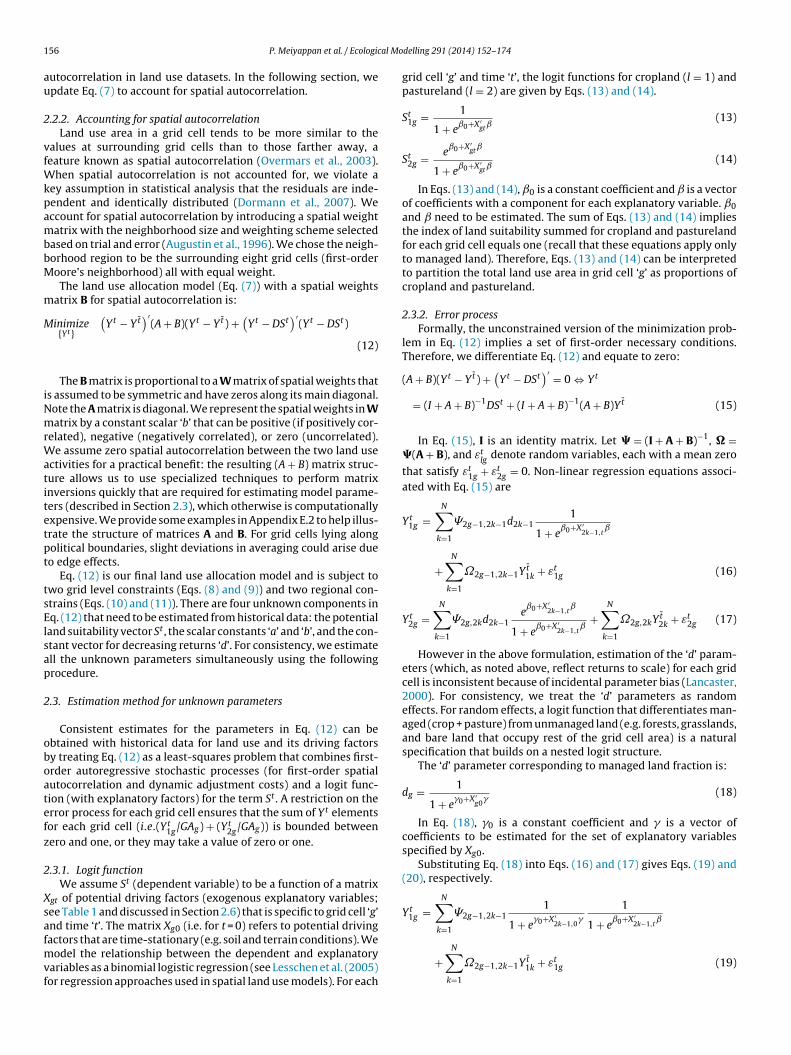
1 al Mo
au
2
vfWkpambbM
m
M
iNmrWatitetpt
tsElsap
2
oboatefz
2
Xsafmvf
56 P. Meiyappan et al. / Ecologic
utocorrelation in land use datasets. In the following section, wepdate Eq. (7) to account for spatial autocorrelation.
.2.2. Accounting for spatial autocorrelationLand use area in a grid cell tends to be more similar to the
alues at surrounding grid cells than to those farther away, aeature known as spatial autocorrelation (Overmars et al., 2003).
hen spatial autocorrelation is not accounted for, we violate aey assumption in statistical analysis that the residuals are inde-endent and identically distributed (Dormann et al., 2007). Weccount for spatial autocorrelation by introducing a spatial weightatrix with the neighborhood size and weighting scheme selected
ased on trial and error (Augustin et al., 1996). We chose the neigh-orhood region to be the surrounding eight grid cells (first-orderoore’s neighborhood) all with equal weight.The land use allocation model (Eq. (7)) with a spatial weights
atrix B for spatial autocorrelation is:
inimize{Yt}
(Yt − Yt
)′(A + B)(Yt − Yt) +
(Yt − DSt
)′(Yt − DSt)
(12)
The B matrix is proportional to a W matrix of spatial weights thats assumed to be symmetric and have zeros along its main diagonal.ote the A matrix is diagonal. We represent the spatial weights in Watrix by a constant scalar ‘b’ that can be positive (if positively cor-
elated), negative (negatively correlated), or zero (uncorrelated).e assume zero spatial autocorrelation between the two land use
ctivities for a practical benefit: the resulting (A + B) matrix struc-ure allows us to use specialized techniques to perform matrixnversions quickly that are required for estimating model parame-ers (described in Section 2.3), which otherwise is computationallyxpensive. We provide some examples in Appendix E.2 to help illus-rate the structure of matrices A and B. For grid cells lying alongolitical boundaries, slight deviations in averaging could arise dueo edge effects.
Eq. (12) is our final land use allocation model and is subject towo grid level constraints (Eqs. (8) and (9)) and two regional con-trains (Eqs. (10) and (11)). There are four unknown components inq. (12) that need to be estimated from historical data: the potentialand suitability vector St , the scalar constants ‘a’ and ‘b’, and the con-tant vector for decreasing returns ‘d’. For consistency, we estimatell the unknown parameters simultaneously using the followingrocedure.
.3. Estimation method for unknown parameters
Consistent estimates for the parameters in Eq. (12) can bebtained with historical data for land use and its driving factorsy treating Eq. (12) as a least-squares problem that combines first-rder autoregressive stochastic processes (for first-order spatialutocorrelation and dynamic adjustment costs) and a logit func-ion (with explanatory factors) for the term St . A restriction on therror process for each grid cell ensures that the sum of Yt elementsor each grid cell (i.e.(Yt
1g/GAg) + (Yt2g/GAg)) is bounded between
ero and one, or they may take a value of zero or one.
.3.1. Logit functionWe assume St (dependent variable) to be a function of a matrix
gt of potential driving factors (exogenous explanatory variables;ee Table 1 and discussed in Section 2.6) that is specific to grid cell ‘g’nd time ‘t’. The matrix Xg0 (i.e. for t = 0) refers to potential driving
actors that are time-stationary (e.g. soil and terrain conditions). Weodel the relationship between the dependent and explanatoryariables as a binomial logistic regression (see Lesschen et al. (2005)or regression approaches used in spatial land use models). For each
delling 291 (2014) 152–174
grid cell ‘g’ and time ‘t’, the logit functions for cropland (l = 1) andpastureland (l = 2) are given by Eqs. (13) and (14).
St1g = 1
1 + eˇ0+X ′
gtˇ(13)
St2g = e
ˇ0+X ′gtˇ
1 + eˇ0+X ′
gtˇ(14)
In Eqs. (13) and (14), ˇ0 is a constant coefficient and is a vectorof coefficients with a component for each explanatory variable. ˇ0and need to be estimated. The sum of Eqs. (13) and (14) impliesthe index of land suitability summed for cropland and pasturelandfor each grid cell equals one (recall that these equations apply onlyto managed land). Therefore, Eqs. (13) and (14) can be interpretedto partition the total land use area in grid cell ‘g’ as proportions ofcropland and pastureland.
2.3.2. Error processFormally, the unconstrained version of the minimization prob-
lem in Eq. (12) implies a set of first-order necessary conditions.Therefore, we differentiate Eq. (12) and equate to zero:
(A + B)(Yt − Yt) +(
Yt − DSt)′ = 0 ⇔ Yt
= (I + A + B)−1DSt + (I + A + B)−1(A + B)Yt (15)
In Eq. (15), I is an identity matrix. Let � = (I + A + B)−1, � =�(A + B), and εt
lgdenote random variables, each with a mean zero
that satisfy εt1g + εt
2g = 0. Non-linear regression equations associ-ated with Eq. (15) are
Yt1g =
N∑k=1
�2g−1,2k−1d2k−11
1 + eˇ0+X ′
2k−1,tˇ
+N∑
k=1
˝2g−1,2k−1Yt1k + εt
1g (16)
Yt2g =
N∑k=1
�2g,2kd2k−1e
ˇ0+X ′2k−1,t
ˇ
1 + eˇ0+X ′
2k−1,tˇ
+N∑
k=1
˝2g,2kY t2k + εt
2g (17)
However in the above formulation, estimation of the ‘d’ param-eters (which, as noted above, reflect returns to scale) for each gridcell is inconsistent because of incidental parameter bias (Lancaster,2000). For consistency, we treat the ‘d’ parameters as randomeffects. For random effects, a logit function that differentiates man-aged (crop + pasture) from unmanaged land (e.g. forests, grasslands,and bare land that occupy rest of the grid cell area) is a naturalspecification that builds on a nested logit structure.
The ‘d’ parameter corresponding to managed land fraction is:
dg = 1
1 + e�0+X ′
g0�
(18)
In Eq. (18), �0 is a constant coefficient and � is a vector ofcoefficients to be estimated for the set of explanatory variablesspecified by Xg0.
Substituting Eq. (18) into Eqs. (16) and (17) gives Eqs. (19) and(20), respectively.
Yt1g =
N∑k=1
�2g−1,2k−11
1 + e�0+X ′
2k−1,0�
1
1 + eˇ0+X ′
2k−1,tˇ
+N∑
k=1
˝2g−1,2k−1Yt1k + εt
1g (19)
al Mo
Y
(eav
twf
t
1
tbaT
ghTasla
Y
2
mm
M
dos
ccats
2
vf
P. Meiyappan et al. / Ecologic
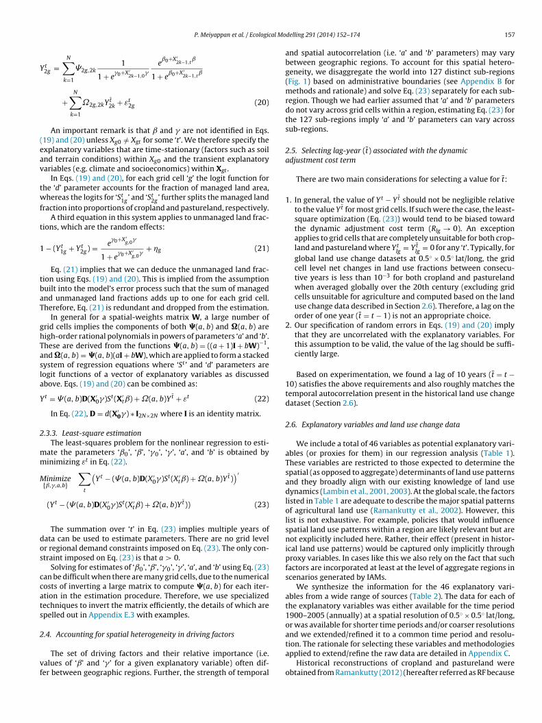
t2g =
N∑k=1
�2g,2k1
1 + e�0+X ′
2k−1,0�
eˇ0+X ′
2k−1,tˇ
1 + eˇ0+X ′
2k−1,tˇ
+N∑
k=1
˝2g,2kY t2k + εt
2g (20)
An important remark is that and � are not identified in Eqs.19) and (20) unless Xg0 /= Xgt for some ‘t’. We therefore specify thexplanatory variables that are time-stationary (factors such as soilnd terrain conditions) within Xg0 and the transient explanatoryariables (e.g. climate and socioeconomics) within Xgt .
In Eqs. (19) and (20), for each grid cell ‘g’ the logit function forhe ‘d’ parameter accounts for the fraction of managed land area,hereas the logits for ‘St
1g ’ and ‘St2g ’ further splits the managed land
raction into proportions of cropland and pastureland, respectively.A third equation in this system applies to unmanaged land frac-
ions, which are the random effects:
− (Yt1g + Yt
2g) = e�0+X ′
g,0�
1 + e�0+X ′
g,0�
+ �g (21)
Eq. (21) implies that we can deduce the unmanaged land frac-ion using Eqs. (19) and (20). This is implied from the assumptionuilt into the model’s error process such that the sum of managednd unmanaged land fractions adds up to one for each grid cell.herefore, Eq. (21) is redundant and dropped from the estimation.
In general for a spatial-weights matrix W, a large number ofrid cells implies the components of both �(a, b) and �(a, b) areigh-order rational polynomials in powers of parameters ‘a’ and ‘b’.hese are derived from the functions �(a, b) = ((a + 1)I + bW)−1,nd �(a, b) = �(a, b)(aI + bW), which are applied to form a stackedystem of regression equations where ‘St ’ and ‘d’ parameters areogit functions of a vector of explanatory variables as discussedbove. Eqs. (19) and (20) can be combined as:
t = � (a, b)D(X′0�)St(X′
tˇ) + ˝(a, b)Yt + εt (22)
In Eq. (22), D = d(X′0�) ∗ I2N×2N where I is an identity matrix.
.3.3. Least-square estimationThe least-squares problem for the nonlinear regression to esti-
ate the parameters ‘ˇ0’, ‘ˇ’, ‘�0’, ‘� ’, ‘a’, and ‘b’ is obtained byinimizing εt in Eq. (22).
inimize{ˇ,�,a,b}
∑t
(Yt − (� (a, b)D(X ′
0�)St(X ′tˇ) + ˝(a, b)Yt)
)′
(Yt − (� (a, b)D(X ′0�)St(X ′
tˇ) + ˝(a, b)Yt)) (23)
The summation over ‘t’ in Eq. (23) implies multiple years ofata can be used to estimate parameters. There are no grid levelr regional demand constraints imposed on Eq. (23). The only con-traint imposed on Eq. (23) is that a > 0.
Solving for estimates of ‘ˇ0’, ‘ˇ’, ‘�0’, ‘� ’, ‘a’, and ‘b’ using Eq. (23)an be difficult when there are many grid cells, due to the numericalosts of inverting a large matrix to compute �(a, b) for each iter-tion in the estimation procedure. Therefore, we use specializedechniques to invert the matrix efficiently, the details of which arepelled out in Appendix E.3 with examples.
.4. Accounting for spatial heterogeneity in driving factors
The set of driving factors and their relative importance (i.e.alues of ‘ˇ’ and ‘� ’ for a given explanatory variable) often dif-er between geographic regions. Further, the strength of temporal
delling 291 (2014) 152–174 157
and spatial autocorrelation (i.e. ‘a’ and ‘b’ parameters) may varybetween geographic regions. To account for this spatial hetero-geneity, we disaggregate the world into 127 distinct sub-regions(Fig. 1) based on administrative boundaries (see Appendix B formethods and rationale) and solve Eq. (23) separately for each sub-region. Though we had earlier assumed that ‘a’ and ‘b’ parametersdo not vary across grid cells within a region, estimating Eq. (23) forthe 127 sub-regions imply ‘a’ and ‘b’ parameters can vary acrosssub-regions.
2.5. Selecting lag-year (t) associated with the dynamicadjustment cost term
There are two main considerations for selecting a value for t:
1. In general, the value of Yt − Yt should not be negligible relativeto the value Yt for most grid cells. If such were the case, the least-square optimization (Eq. (23)) would tend to be biased towardthe dynamic adjustment cost term (Rlg → 0). An exceptionapplies to grid cells that are completely unsuitable for both crop-land and pastureland where Yt
lg= Yt
lg= 0 for any ‘t’. Typically, for
global land use change datasets at 0.5◦ × 0.5◦ lat/long, the gridcell level net changes in land use fractions between consecu-tive years is less than 10−3 for both cropland and pasturelandwhen averaged globally over the 20th century (excluding gridcells unsuitable for agriculture and computed based on the landuse change data described in Section 2.6). Therefore, a lag on theorder of one year (t = t − 1) is not an appropriate choice.
2. Our specification of random errors in Eqs. (19) and (20) implythat they are uncorrelated with the explanatory variables. Forthis assumption to be valid, the value of the lag should be suffi-ciently large.
Based on experimentation, we found a lag of 10 years (t = t −10) satisfies the above requirements and also roughly matches thetemporal autocorrelation present in the historical land use changedataset (Section 2.6).
2.6. Explanatory variables and land use change data
We include a total of 46 variables as potential explanatory vari-ables (or proxies for them) in our regression analysis (Table 1).These variables are restricted to those expected to determine thespatial (as opposed to aggregate) determinants of land use patternsand they broadly align with our existing knowledge of land usedynamics (Lambin et al., 2001, 2003). At the global scale, the factorslisted in Table 1 are adequate to describe the major spatial patternsof agricultural land use (Ramankutty et al., 2002). However, thislist is not exhaustive. For example, policies that would influencespatial land use patterns within a region are likely relevant but arenot explicitly included here. Rather, their effect (present in histor-ical land use patterns) would be captured only implicitly throughproxy variables. In cases like this we also rely on the fact that suchfactors are incorporated at least at the level of aggregate regions inscenarios generated by IAMs.
We synthesize the information for the 46 explanatory vari-ables from a wide range of sources (Table 2). The data for each ofthe explanatory variables was either available for the time period1900–2005 (annually) at a spatial resolution of 0.5◦ × 0.5◦ lat/long,or was available for shorter time periods and/or coarser resolutionsand we extended/refined it to a common time period and resolu-
tion. The rationale for selecting these variables and methodologiesapplied to extend/refine the raw data are detailed in Appendix C.Historical reconstructions of cropland and pastureland wereobtained from Ramankutty (2012) (hereafter referred as RF because
158 P. Meiyappan et al. / Ecological Modelling 291 (2014) 152–174
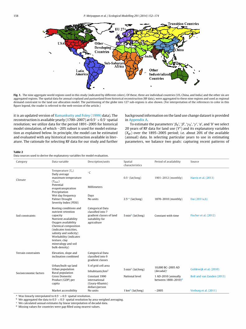
Fig. 1. The nine aggregate world regions used in this study (indicated by different colors). Of these, three are individual countries (US, China, and India) and the other six area rical rd into 1fi
irrmtaa
TD
ggregated regions. The spatial data for annual cropland and pastureland from histoemand constraint to the land use allocation model. The partitioning of the globe
gure legend, the reader is referred to the web version of the article.)
t is an updated version of Ramankutty and Foley (1999) data). Theeconstruction is available yearly (1700–2007) at 0.5◦ × 0.5◦ spatialesolution; we utilize data for the period 1891–2005 for historical
odel simulation, of which ∼20% subset is used for model estima-ion as explained below. In principle, the model can be estimatednd evaluated with any historical reconstruction available in liter-ture. The rationale for selecting RF data for our study and further
able 2ata sources used to derive the explanatory variables for model evaluation.
Category Data variable Description/units Sc
Climate
Temperature (Ta) ◦C
0Daily averagemaximum temperature(Tmax)Potentialevapotranspiration Millimeters
PrecipitationWet day frequency DaysPalmer DroughtSeverity Index (PDSI)
No units 2
Soil constraints
Rooting conditions andnutrient retentioncapacity
Categorical Dataclassified into 7gradient classes of landsuitability foragriculture
5Nutrient availabilityOxygen availabilityChemical composition(indicates toxicities,salinity and sodicity)Workability (indicatestexture, claymineralogy and soilbulk-density)
Terrain constraints Elevation, slope andinclination combined
Categorical Dataclassified into 9gradient classes
Socioeconomic factors
Urban/built-up land % of grid cell area5Urban population
Inhabitants/km2Rural populationGross DomesticProduct (GDP) percapita
Constant 1990international(Geary-Khamis)dollars/person
N
Market accessibility No units 1
a Was linearly interpolated to 0.5◦ × 0.5◦ spatial resolution.b We aggregated the data to 0.5◦ × 0.5◦ spatial resolution by area-weighed averaging.c We calculated annual estimates by linear interpolation of decadal data.d Missing values for countries were gap filled using nearest values.
econstruction (RF data), were aggregated to these nine regions and used as regional27 sub-regions is also shown. (For interpretation of the references to color in this
background information on the land use change dataset is providedin Appendix A.
To estimate the parameters ‘ˇ0’, ‘ˇ’, ‘�0’, ‘� ’, ‘a’, and ‘b’ we select
20 years of RF data for land use (Yt) and its explanatory variables(Xgt) over the 1895–2005 period; i.e. about 20% of the available(annual) data. In selecting particular years to use in estimatingparameters, we balance two goals: capturing recent patterns ofpatialharacteristics
Period of availability Source
.5◦ (lat/long) 1901–2012 (monthly) Harris et al. (2013)
.5◦a (lat/long) 1870–2010 (monthly) Dai (2011a,b)
minb (lat/long) Constant with time Fischer et al. (2012)
minb (lat/long)10,000 BC–2005 AD(decadal)c Goldewijk et al. (2010)
ational level 1 AD-2010 (annuallybetween 1800–2010)d
Bolt and van Zanden (2013)
kmb (lat/long) ∼2005 Verburg et al. (2011)
al Modelling 291 (2014) 152–174 159
lltWtayelcta1
f(ptatsdAtiF�dgattc
tpis
2m
ftttgmsm1drtrucutswe
gr
P. Meiyappan et al. / Ecologic
and use from which future projections will begin, and capturingarger, longer-term changes in land use and explanatory variableso better support use of the model in long-term future projections.
e therefore choose two 10-year sets of data. The first set, to cap-ure longer-term changes, consists of 10 years drawn between 1905nd 1995 at 10-year time steps (i.e. 1905, 1915,. . ., 1995). For eachear, a corresponding 10-year lag data point (Yt−10) is used in thestimation procedure (Section 2.5). For example, for year 1905, theag year data corresponds to 1895, and for 1995 the lag year dataorresponds to 1985. The second set, to capture contemporary rela-ionships, includes 10 years of data covering the period 1996–2005t 1-year time steps. For 1996, the lag year data corresponds to986, and for 2005 the lag year data corresponds to 1995.
The explanatory variables (Table 1) used in the analysis have dif-erent units and scales. Hence, the estimated regression coefficients
and � vectors) are of different scale and cannot be directly inter-reted to infer the relative importance of explanatory variables onhe dependent variable. To address this problem, we standardizell explanatory variables covering the period 1901–2005 beforehe parameter estimation and model simulation procedure. Thetandardization also prevents numerical difficulties that could ariseue to scaling problems in the least-squares estimation (Eq. (23)).
standardized coefficient indicates how many standard devia-ions a dependent variable will change, per standard deviationncrease in the explanatory variable (Hunter and Hamilton, 2002).or each explanatory variable associated with the vectors and, we calculate its mean and standard deviation using 5 years ofata (2001–2005) separately for each of the 127 sub-region. For aiven explanatory variable and grid cell, we standardize the vari-ble using the z-score which is computed as the difference betweenhe value of the variable at that grid cell and its mean value forhe corresponding sub-region, divided by the standard deviationorresponding to that sub-region.
See Appendix D for a discussion on how we handle mul-icollinearity among explanatory variables and excess-zerosroblem. Appendix E.4 provides details on the solvers used to
mplement the land use allocation model (Eq. (12)) and the least-quares optimization (Eq. (23)).
.7. Simulation procedure to evaluate the land use allocationodel
To test the land use allocation model, we compared resultsrom model simulations for the historical period (1901–2005) tohe historical reconstruction (RF data) over that period. For thisest, we first divided the world into nine regions (Fig. 1), consis-ent with the regions used in a general equilibrium model of thelobal economy, the PET (Population-Environment-Technology)odel (O’Neill et al., 2010). This regional mask will allow us to
ubsequently link the land use allocation model with the PETodel for exploring future scenarios. For each year over the period
901–2005, we aggregated the 0.5◦ × 0.5◦ lat/long reconstructionata for cropland and pastureland to these nine regions. Thisegionally aggregated land use information was then used as inputo the land use allocation model (Eq. (12)) to form the annualegional-scale constraint on the total area demand for each landse type (through Eqs. (10) and (11)). Next, the land use allo-ation model (Eq. (12)) allocated the regionally aggregated landse information back to 0.5◦ × 0.5◦ spatial resolution by applyingime-dependent regional demand constraints and two local con-traints (Eqs. (8) and (9)). The model-downscaled land use mapsere finally compared to the original 0.5◦ × 0.5◦ lat/long RF data to
valuate model performance.Our evaluation test is rigorous given that most IAMs disaggre-
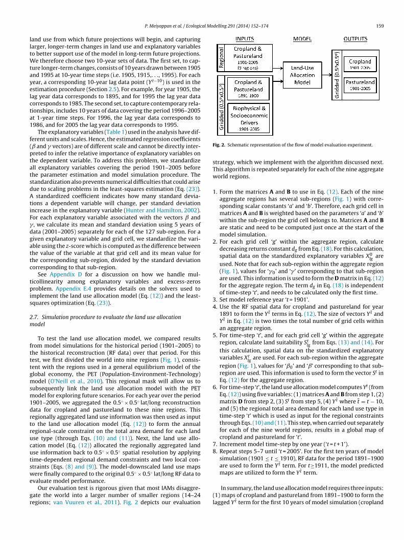
ate the world into a larger number of smaller regions (14–24egions; van Vuuren et al., 2011). Fig. 2 depicts our evaluation
Fig. 2. Schematic representation of the flow of model evaluation experiment.
strategy, which we implement with the algorithm discussed next.This algorithm is repeated separately for each of the nine aggregateworld regions.
1. Form the matrices A and B to use in Eq. (12). Each of the nineaggregate regions has several sub-regions (Fig. 1) with corre-sponding scalar constants ‘a’ and ‘b’. Therefore, each grid cell inmatrices A and B is weighted based on the parameters ‘a’ and ‘b’within the sub-region the grid cell belongs to. Matrices A and Bare static and need to be computed just once at the start of themodel simulation.
2. For each grid cell ‘g’ within the aggregate region, calculatedecreasing returns constant dg from Eq. (18). For this calculation,spatial data on the standardized explanatory variables X0
lgare
used. Note that for each sub-region within the aggregate region(Fig. 1), values for ‘�0’ and ‘� ’ corresponding to that sub-regionare used. This information is used to form the D matrix in Eq. (12)for the aggregate region. The term dg in Eq. (18) is independentof time-step ‘t’, and needs to be calculated only the first time.
3. Set model reference year ‘t = 1901’.4. Use the RF spatial data for cropland and pastureland for year
1891 to form the Yt terms in Eq. (12). The size of vectors Yt andYt in Eq. (12) is two times the total number of grid cells withinan aggregate region.
5. For time-step ‘t’, and for each grid cell ‘g’ within the aggregateregion, calculate land suitability St
lgfrom Eqs. (13) and (14). For
this calculation, spatial data on the standardized explanatoryvariables Xt
lgare used. For each sub-region within the aggregate
region (Fig. 1), values for ‘ˇ0’ and ‘ˇ’ corresponding to that sub-region are used. This information is used to form the vector St inEq. (12) for the aggregate region.
6. For time-step ‘t’, the land use allocation model computes Yt (fromEq. (12)) using five variables: (1) matrices A and B from step 1, (2)matrix D from step 2, (3) St from step 5, (4) Yt where t = t − 10,and (5) the regional total area demand for each land use type intime-step ‘t’ which is used as input for the regional constraintsthrough Eqs. (10) and (11). This step, when carried out separatelyfor each of the nine world regions, results in a global map ofcropland and pastureland for ‘t’.
7. Increment model time-step by one year (‘t = t + 1’).8. Repeat steps 5–7 until ‘t = 2005’. For the first ten years of model
simulation (1901 ≤ t ≤ 1910), RF data for the period 1891–1900are used to form the Yt term. For t≥1911, the model predictedmaps are utilized to form the Yt term.
In summary, the land use allocation model requires three inputs:(1) maps of cropland and pastureland from 1891–1900 to form thelagged Yt term for the first 10 years of model simulation (cropland
160 P. Meiyappan et al. / Ecological Modelling 291 (2014) 152–174
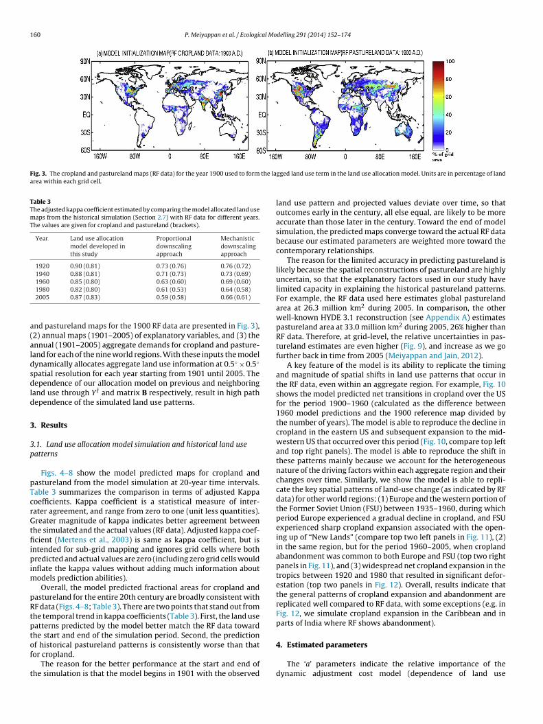
Fig. 3. The cropland and pastureland maps (RF data) for the year 1900 used to form the laarea within each grid cell.
Table 3The adjusted kappa coefficient estimated by comparing the model allocated land usemaps from the historical simulation (Section 2.7) with RF data for different years.The values are given for cropland and pastureland (brackets).
Year Land use allocationmodel developed inthis study
Proportionaldownscalingapproach
Mechanisticdownscalingapproach
1920 0.90 (0.81) 0.73 (0.76) 0.76 (0.72)1940 0.88 (0.81) 0.71 (0.73) 0.73 (0.69)1960 0.85 (0.80) 0.63 (0.60) 0.69 (0.60)
a(aldsdld
3
3p
pTcrGtfiipim
pRtptof
t
1980 0.82 (0.80) 0.61 (0.53) 0.64 (0.58)2005 0.87 (0.83) 0.59 (0.58) 0.66 (0.61)
nd pastureland maps for the 1900 RF data are presented in Fig. 3),2) annual maps (1901–2005) of explanatory variables, and (3) thennual (1901–2005) aggregate demands for cropland and pasture-and for each of the nine world regions. With these inputs the modelynamically allocates aggregate land use information at 0.5◦ × 0.5◦
patial resolution for each year starting from 1901 until 2005. Theependence of our allocation model on previous and neighboring
and use through Yt and matrix B respectively, result in high pathependence of the simulated land use patterns.
. Results
.1. Land use allocation model simulation and historical land useatterns
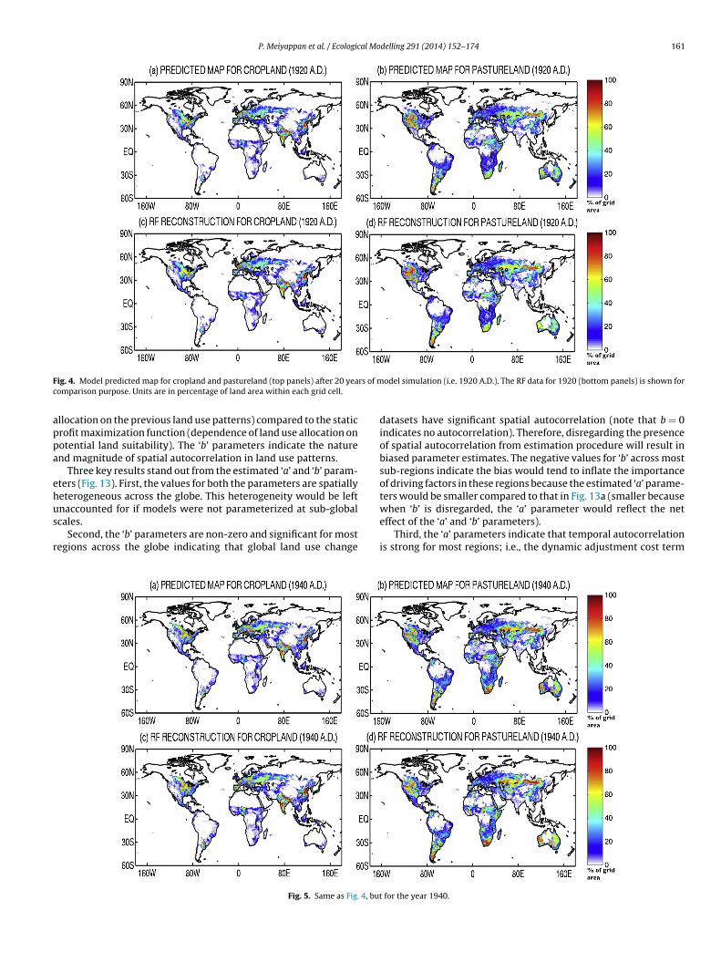
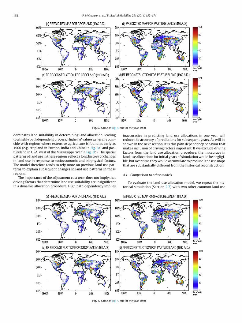
Figs. 4–8 show the model predicted maps for cropland andastureland from the model simulation at 20-year time intervals.able 3 summarizes the comparison in terms of adjusted Kappaoefficients. Kappa coefficient is a statistical measure of inter-ater agreement, and range from zero to one (unit less quantities).reater magnitude of kappa indicates better agreement between
he simulated and the actual values (RF data). Adjusted kappa coef-cient (Mertens et al., 2003) is same as kappa coefficient, but is
ntended for sub-grid mapping and ignores grid cells where bothredicted and actual values are zero (including zero grid cells would
nflate the kappa values without adding much information aboutodels prediction abilities).Overall, the model predicted fractional areas for cropland and
astureland for the entire 20th century are broadly consistent withF data (Figs. 4–8; Table 3). There are two points that stand out fromhe temporal trend in kappa coefficients (Table 3). First, the land useatterns predicted by the model better match the RF data towardhe start and end of the simulation period. Second, the prediction
f historical pastureland patterns is consistently worse than thator cropland.The reason for the better performance at the start and end ofhe simulation is that the model begins in 1901 with the observed
gged land use term in the land use allocation model. Units are in percentage of land
land use pattern and projected values deviate over time, so thatoutcomes early in the century, all else equal, are likely to be moreaccurate than those later in the century. Toward the end of modelsimulation, the predicted maps converge toward the actual RF databecause our estimated parameters are weighted more toward thecontemporary relationships.
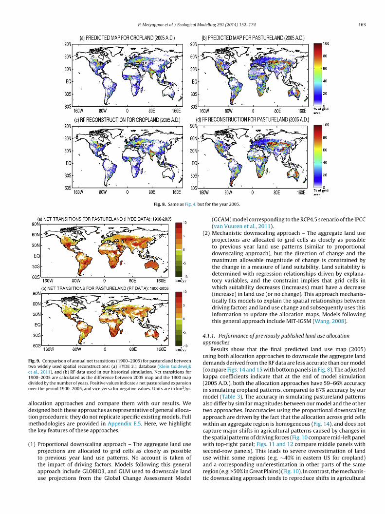
The reason for the limited accuracy in predicting pastureland islikely because the spatial reconstructions of pastureland are highlyuncertain, so that the explanatory factors used in our study havelimited capacity in explaining the historical pastureland patterns.For example, the RF data used here estimates global pasturelandarea at 26.3 million km2 during 2005. In comparison, the otherwell-known HYDE 3.1 reconstruction (see Appendix A) estimatespastureland area at 33.0 million km2 during 2005, 26% higher thanRF data. Therefore, at grid-level, the relative uncertainties in pas-tureland estimates are even higher (Fig. 9), and increase as we gofurther back in time from 2005 (Meiyappan and Jain, 2012).
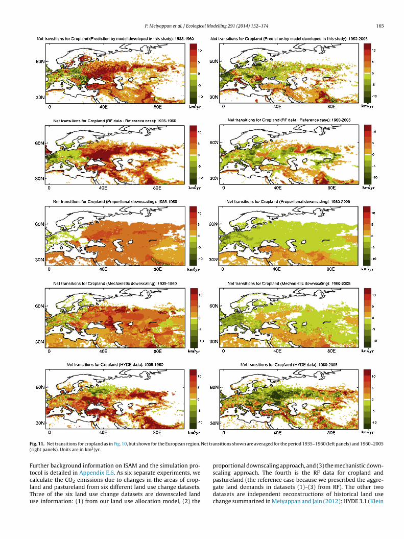
A key feature of the model is its ability to replicate the timingand magnitude of spatial shifts in land use patterns that occur inthe RF data, even within an aggregate region. For example, Fig. 10shows the model predicted net transitions in cropland over the USfor the period 1900–1960 (calculated as the difference between1960 model predictions and the 1900 reference map divided bythe number of years). The model is able to reproduce the decline incropland in the eastern US and subsequent expansion to the mid-western US that occurred over this period (Fig. 10, compare top leftand top right panels). The model is able to reproduce the shift inthese patterns mainly because we account for the heterogeneousnature of the driving factors within each aggregate region and theirchanges over time. Similarly, we show the model is able to repli-cate the key spatial patterns of land-use change (as indicated by RFdata) for other world regions: (1) Europe and the western portion ofthe Former Soviet Union (FSU) between 1935–1960, during whichperiod Europe experienced a gradual decline in cropland, and FSUexperienced sharp cropland expansion associated with the open-ing up of “New Lands” (compare top two left panels in Fig. 11), (2)in the same region, but for the period 1960–2005, when croplandabandonment was common to both Europe and FSU (top two rightpanels in Fig. 11), and (3) widespread net cropland expansion in thetropics between 1920 and 1980 that resulted in significant defor-estation (top two panels in Fig. 12). Overall, results indicate thatthe general patterns of cropland expansion and abandonment arereplicated well compared to RF data, with some exceptions (e.g. inFig. 12, we simulate cropland expansion in the Caribbean and inparts of India where RF shows abandonment).
4. Estimated parameters
The ‘a’ parameters indicate the relative importance of thedynamic adjustment cost model (dependence of land use
P. Meiyappan et al. / Ecological Modelling 291 (2014) 152–174 161
F rs of mc
appa
ehus
r
ig. 4. Model predicted map for cropland and pastureland (top panels) after 20 yeaomparison purpose. Units are in percentage of land area within each grid cell.
llocation on the previous land use patterns) compared to the staticrofit maximization function (dependence of land use allocation onotential land suitability). The ‘b’ parameters indicate the naturend magnitude of spatial autocorrelation in land use patterns.
Three key results stand out from the estimated ‘a’ and ‘b’ param-ters (Fig. 13). First, the values for both the parameters are spatiallyeterogeneous across the globe. This heterogeneity would be leftnaccounted for if models were not parameterized at sub-global
cales.Second, the ‘b’ parameters are non-zero and significant for mostegions across the globe indicating that global land use change
Fig. 5. Same as Fig. 4, but
odel simulation (i.e. 1920 A.D.). The RF data for 1920 (bottom panels) is shown for
datasets have significant spatial autocorrelation (note that b = 0indicates no autocorrelation). Therefore, disregarding the presenceof spatial autocorrelation from estimation procedure will result inbiased parameter estimates. The negative values for ‘b’ across mostsub-regions indicate the bias would tend to inflate the importanceof driving factors in these regions because the estimated ‘a’ parame-ters would be smaller compared to that in Fig. 13a (smaller becausewhen ‘b’ is disregarded, the ‘a’ parameter would reflect the net
effect of the ‘a’ and ‘b’ parameters).Third, the ‘a’ parameters indicate that temporal autocorrelationis strong for most regions; i.e., the dynamic adjustment cost term
for the year 1940.
162 P. Meiyappan et al. / Ecological Modelling 291 (2014) 152–174
4, but
dtc1tpiTtr
di
Fig. 6. Same as Fig.
ominates land suitability in determining land allocation, leadingo a highly path dependent process. Higher ‘a’ values generally coin-ide with regions where extensive agriculture is found as early as900 (e.g. cropland in Europe, India and China in Fig. 3a, and pas-ureland in USA, west of the Mississippi river in Fig. 3b). The spatialatterns of land use in these regions reflect a long history of changes
n land use in response to socioeconomic and biophysical factors.he model therefore tends to rely more on previous land use pat-erns to explain subsequent changes in land use patterns in these
egions.The importance of the adjustment cost term does not imply thatriving factors that determine land use suitability are insignificant
n a dynamic allocation procedure. High path dependency implies
Fig. 7. Same as Fig. 4, but
for the year 1960.
inaccuracies in predicting land use allocations in one year willreduce the accuracy of predictions for subsequent years. As will beshown in the next section, it is this path dependency behavior thatmakes inclusion of driving factors important. If we exclude drivingfactors from the land use allocation procedure, the inaccuracy inland use allocations for initial years of simulation would be negligi-ble, but over time they would accumulate to produce land use mapsthat are substantially different from the historical reconstruction.
4.1. Comparison to other models
To evaluate the land use allocation model, we repeat the his-torical simulation (Section 2.7) with two other common land use
for the year 1980.
P. Meiyappan et al. / Ecological Modelling 291 (2014) 152–174 163
Fig. 8. Same as Fig. 4, but
Fig. 9. Comparison of annual net transitions (1900–2005) for pastureland betweentwo widely used spatial reconstructions: (a) HYDE 3.1 database (Klein Goldewijket al., 2011), and (b) RF data used in our historical simulation. Net transitions for1do
adtmt
(
900–2005 are calculated as the difference between 2005 map and the 1900 mapivided by the number of years. Positive values indicate a net pastureland expansionver the period 1900–2005, and vice versa for negative values. Units are in km2/yr.
llocation approaches and compare them with our results. Weesigned both these approaches as representative of general alloca-ion procedures; they do not replicate specific existing models. Full
ethodologies are provided in Appendix E.5. Here, we highlighthe key features of these approaches.
1) Proportional downscaling approach – The aggregate land useprojections are allocated to grid cells as closely as possible
to previous year land use patterns. No account is taken ofthe impact of driving factors. Models following this generalapproach include GLOBIO3, and GLM used to downscale landuse projections from the Global Change Assessment Modelfor the year 2005.
(GCAM) model corresponding to the RCP4.5 scenario of the IPCC(van Vuuren et al., 2011).
(2) Mechanistic downscaling approach – The aggregate land useprojections are allocated to grid cells as closely as possibleto previous year land use patterns (similar to proportionaldownscaling approach), but the direction of change and themaximum allowable magnitude of change is constrained bythe change in a measure of land suitability. Land suitability isdetermined with regression relationships driven by explana-tory variables, and the constraint implies that grid cells inwhich suitability decreases (increases) must have a decrease(increase) in land use (or no change). This approach mechanis-tically fits models to explain the spatial relationships betweendriving factors and land use change and subsequently uses thisinformation to update the allocation maps. Models followingthis general approach include MIT-IGSM (Wang, 2008).
4.1.1. Performance of previously published land use allocationapproaches
Results show that the final predicted land use map (2005)using both allocation approaches to downscale the aggregate landdemands derived from the RF data are less accurate than our model(compare Figs. 14 and 15 with bottom panels in Fig. 8). The adjustedkappa coefficients indicate that at the end of model simulation(2005 A.D.), both the allocation approaches have 59–66% accuracyin simulating cropland patterns, compared to 87% accuracy by ourmodel (Table 3). The accuracy in simulating pastureland patternsalso differ by similar magnitudes between our model and the othertwo approaches. Inaccuracies using the proportional downscalingapproach are driven by the fact that the allocation across grid cellswithin an aggregate region is homogeneous (Fig. 14), and does notcapture major shifts in agricultural patterns caused by changes inthe spatial patterns of driving forces (Fig. 10 compare mid-left panelwith top-right panel; Figs. 11 and 12 compare middle panels withsecond-row panels). This leads to severe overestimation of land
use within some regions (e.g. ∼40% in eastern US for cropland)and a corresponding underestimation in other parts of the sameregion (e.g. >50% in Great Plains) (Fig. 10). In contrast, the mechanis-tic downscaling approach tends to reproduce shifts in agricultural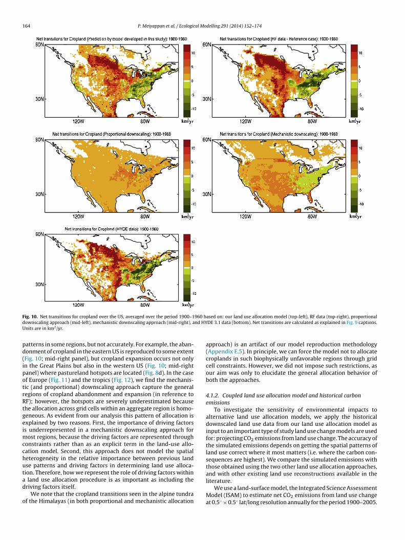
164 P. Meiyappan et al. / Ecological Modelling 291 (2014) 152–174
F 960 bd nd HYU
pd(ipotrRtgeimcchutad
o
ig. 10. Net transitions for cropland over the US, averaged over the period 1900–1ownscaling approach (mid-left), mechanistic downscaling approach (mid-right), anits are in km2/yr.
atterns in some regions, but not accurately. For example, the aban-onment of cropland in the eastern US is reproduced to some extentFig. 10; mid-right panel), but cropland expansion occurs not onlyn the Great Plains but also in the western US (Fig. 10; mid-rightanel) where pastureland hotspots are located (Fig. 8d). In the casef Europe (Fig. 11) and the tropics (Fig. 12), we find the mechanis-ic (and proportional) downscaling approach capture the generalegions of cropland abandonment and expansion (in reference toF); however, the hotspots are severely underestimated becausehe allocation across grid cells within an aggregate region is homo-eneous. As evident from our analysis this pattern of allocation isxplained by two reasons. First, the importance of driving factorss underrepresented in a mechanistic downscaling approach for
ost regions, because the driving factors are represented throughonstraints rather than as an explicit term in the land-use allo-ation model. Second, this approach does not model the spatialeterogeneity in the relative importance between previous landse patterns and driving factors in determining land use alloca-ion. Therefore, how we represent the role of driving factors within
land use allocation procedure is as important as including theriving factors itself.
We note that the cropland transitions seen in the alpine tundraf the Himalayas (in both proportional and mechanistic allocation
ased on: our land use allocation model (top-left), RF data (top-right), proportionalDE 3.1 data (bottom). Net transitions are calculated as explained in Fig. 9 captions.
approach) is an artifact of our model reproduction methodology(Appendix E.5). In principle, we can force the model not to allocatecroplands in such biophysically unfavorable regions through gridcell constraints. However, we did not impose such restrictions, asour aim was only to elucidate the general allocation behavior ofboth the approaches.
4.1.2. Coupled land use allocation model and historical carbonemissions
To investigate the sensitivity of environmental impacts toalternative land use allocation models, we apply the historicaldownscaled land use data from our land use allocation model asinput to an important type of study land use change models are usedfor: projecting CO2 emissions from land use change. The accuracy ofthe simulated emissions depends on getting the spatial patterns ofland use correct where it most matters (i.e. where the carbon con-sequences are highest). We compare the simulated emissions withthose obtained using the two other land use allocation approaches,and with other existing land use reconstructions available in the
literature.We use a land-surface model, the Integrated Science AssessmentModel (ISAM) to estimate net CO2 emissions from land use changeat 0.5◦ × 0.5◦ lat/long resolution annually for the period 1900–2005.
P. Meiyappan et al. / Ecological Modelling 291 (2014) 152–174 165
F Net tra(
FtclTu
ig. 11. Net transitions for cropland as in Fig. 10, but shown for the European region.
right panels). Units are in km2/yr.
urther background information on ISAM and the simulation pro-ocol is detailed in Appendix E.6. As six separate experiments, we
alculate the CO2 emissions due to changes in the areas of crop-and and pastureland from six different land use change datasets.hree of the six land use change datasets are downscaled landse information: (1) from our land use allocation model, (2) thensitions shown are averaged for the period 1935–1960 (left panels) and 1960–2005
proportional downscaling approach, and (3) the mechanistic down-scaling approach. The fourth is the RF data for cropland and
pastureland (the reference case because we prescribed the aggre-gate land demands in datasets (1)–(3) from RF). The other twodatasets are independent reconstructions of historical land usechange summarized in Meiyappan and Jain (2012): HYDE 3.1 (Klein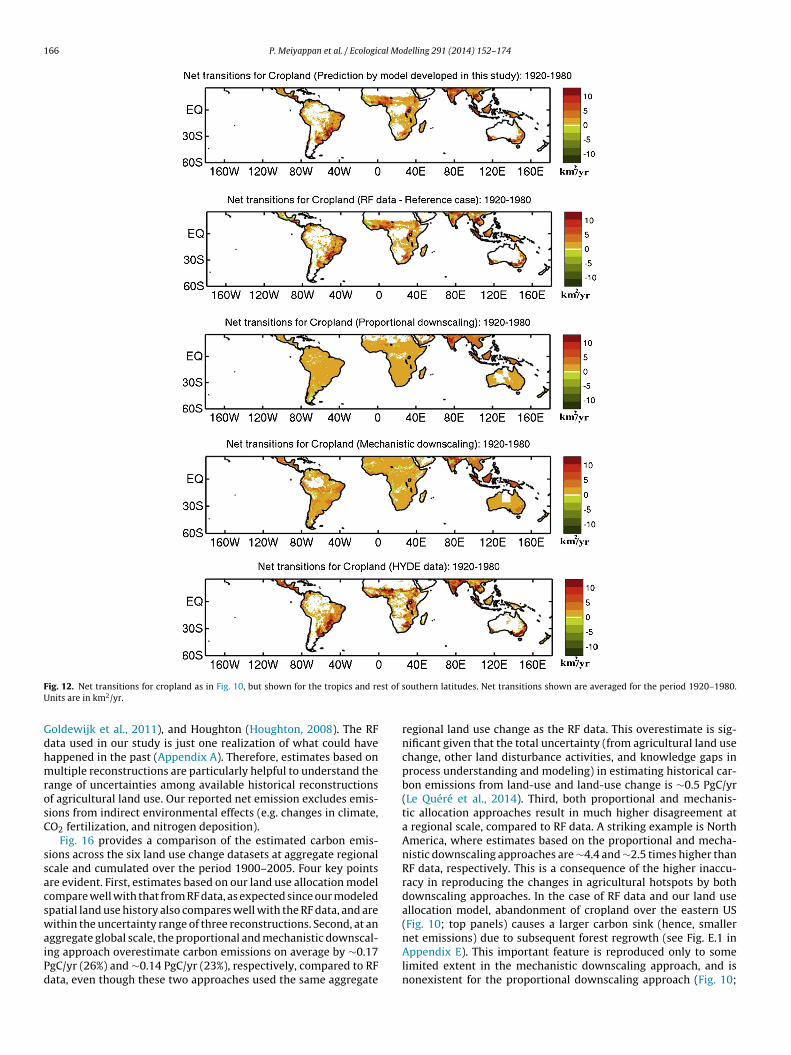
166 P. Meiyappan et al. / Ecological Modelling 291 (2014) 152–174
F st of sU
GdhmrosC
ssacswaiPd
ig. 12. Net transitions for cropland as in Fig. 10, but shown for the tropics and renits are in km2/yr.
oldewijk et al., 2011), and Houghton (Houghton, 2008). The RFata used in our study is just one realization of what could haveappened in the past (Appendix A). Therefore, estimates based onultiple reconstructions are particularly helpful to understand the
ange of uncertainties among available historical reconstructionsf agricultural land use. Our reported net emission excludes emis-ions from indirect environmental effects (e.g. changes in climate,O2 fertilization, and nitrogen deposition).
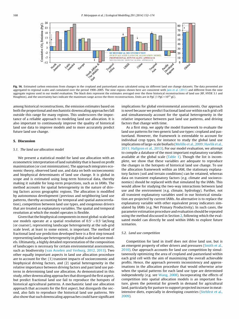
Fig. 16 provides a comparison of the estimated carbon emis-ions across the six land use change datasets at aggregate regionalcale and cumulated over the period 1900–2005. Four key pointsre evident. First, estimates based on our land use allocation modelompare well with that from RF data, as expected since our modeledpatial land use history also compares well with the RF data, and areithin the uncertainty range of three reconstructions. Second, at an
ggregate global scale, the proportional and mechanistic downscal-ng approach overestimate carbon emissions on average by ∼0.17gC/yr (26%) and ∼0.14 PgC/yr (23%), respectively, compared to RFata, even though these two approaches used the same aggregate
outhern latitudes. Net transitions shown are averaged for the period 1920–1980.
regional land use change as the RF data. This overestimate is sig-nificant given that the total uncertainty (from agricultural land usechange, other land disturbance activities, and knowledge gaps inprocess understanding and modeling) in estimating historical car-bon emissions from land-use and land-use change is ∼0.5 PgC/yr(Le Quéré et al., 2014). Third, both proportional and mechanis-tic allocation approaches result in much higher disagreement ata regional scale, compared to RF data. A striking example is NorthAmerica, where estimates based on the proportional and mecha-nistic downscaling approaches are ∼4.4 and ∼2.5 times higher thanRF data, respectively. This is a consequence of the higher inaccu-racy in reproducing the changes in agricultural hotspots by bothdownscaling approaches. In the case of RF data and our land useallocation model, abandonment of cropland over the eastern US(Fig. 10; top panels) causes a larger carbon sink (hence, smaller
net emissions) due to subsequent forest regrowth (see Fig. E.1 inAppendix E). This important feature is reproduced only to somelimited extent in the mechanistic downscaling approach, and isnonexistent for the proportional downscaling approach (Fig. 10;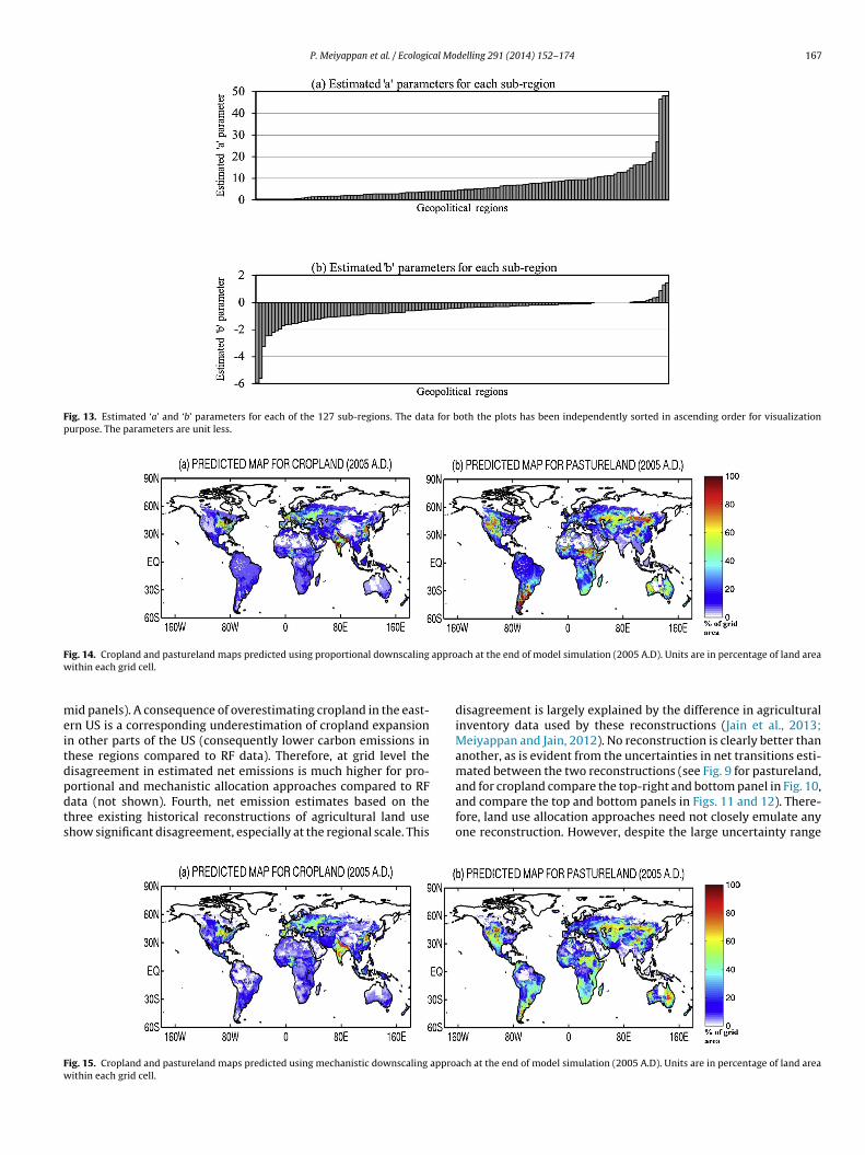
P. Meiyappan et al. / Ecological Modelling 291 (2014) 152–174 167
Fig. 13. Estimated ‘a’ and ‘b’ parameters for each of the 127 sub-regions. The data for both the plots has been independently sorted in ascending order for visualizationpurpose. The parameters are unit less.
F approw
meitdpdts
Fw
ig. 14. Cropland and pastureland maps predicted using proportional downscalingithin each grid cell.
id panels). A consequence of overestimating cropland in the east-rn US is a corresponding underestimation of cropland expansionn other parts of the US (consequently lower carbon emissions inhese regions compared to RF data). Therefore, at grid level theisagreement in estimated net emissions is much higher for pro-
ortional and mechanistic allocation approaches compared to RFata (not shown). Fourth, net emission estimates based on thehree existing historical reconstructions of agricultural land usehow significant disagreement, especially at the regional scale. Thisig. 15. Cropland and pastureland maps predicted using mechanistic downscaling approithin each grid cell.
ach at the end of model simulation (2005 A.D). Units are in percentage of land area
disagreement is largely explained by the difference in agriculturalinventory data used by these reconstructions (Jain et al., 2013;Meiyappan and Jain, 2012). No reconstruction is clearly better thananother, as is evident from the uncertainties in net transitions esti-mated between the two reconstructions (see Fig. 9 for pastureland,
and for cropland compare the top-right and bottom panel in Fig. 10,and compare the top and bottom panels in Figs. 11 and 12). There-fore, land use allocation approaches need not closely emulate anyone reconstruction. However, despite the large uncertainty rangeach at the end of model simulation (2005 A.D). Units are in percentage of land area
168 P. Meiyappan et al. / Ecological Modelling 291 (2014) 152–174
Fig. 16. Estimated carbon emissions from changes in the cropland and pastureland areas calculated using six different land use change datasets. The data presented area e regia matesH recon
abotalf
5
5
emnasmmibpttr
u(sfreosoabrtsbhaoa
ggregated to regional scales and cumulated over the period 1900–2005. The ninggregate regions used in our model evaluation. The black dots represent the estioughton), and the uncertainty bars indicate the maximum range across the three
mong historical reconstructions, the emission estimates based onoth the proportional and mechanistic downscaling approaches fallutside this range for many regions. This underscores the impor-ance of a reliable approach to modeling land use allocation. It islso important to continuously improve the quality of historicaland use data to improve models and to more accurately predictuture land use change.
. Discussion
.1. The land use allocation model
We present a statistical model for land use allocation with anconometric interpretation of land suitability that is based on profitaximization (or cost minimization). The approach integrates eco-
omic theory, observed land use, and data on both socioeconomicnd biophysical determinants of land use change. It is global incope and is estimated using long-term historical data, therebyaking it suitable for long-term projections, such as in IAMs. Theethod accounts for spatial heterogeneity in the nature of driv-
ng factors across geographic regions. The allocation is modifiedy autonomous development (previous and neighboring land useatterns, thereby accounting for temporal and spatial autocorrela-ion), competition between land use types, and exogenous drivershat are treated as explanatory variables. The spatial and temporalesolution at which the model operates is flexible.
Given that the biophysical components in most global-scale landse models operate at a spatial resolution of 0.5◦ × 0.5◦ lat/longor coarser), representing landscape heterogeneity at the sub-gridcale level, at least to some extent, is important. The method ofractional land use prediction developed here is a first step towardepresenting landscape heterogeneity in global scale land use mod-ls. Ultimately, a highly detailed representation of the compositionf landscapes is necessary for certain environmental assessments,uch as biodiversity (van Asselen and Verburg, 2012, 2013). Twother equally important aspects in land use allocation procedurere to account for the: (1) transient impacts of socioeconomic andiophysical driving factors, and (2) spatial heterogeneity in theelative importance between driving factors and past land use pat-erns in determining land use allocation. As demonstrated in thistudy, other downscaling approaches that disregard the first aspect,ut predict fractional land use fail to reproduce the hotspots of
istorical agricultural patterns. A mechanistic land use allocationpproach that accounts for the first aspect, but disregards the sec-nd, also fails to reproduce the historical land use patterns. Welso show that such downscaling approaches could have significantons shown here are consistent with Jain et al. (2013) and different from the nine averaged over the three historical reconstructions of land use (RF, HYDE 3.1 andstructions. Units are in PgC (1 PgC = 1015 gC).
implications for global environmental assessments. Our approachis novel because we predict fractional land use within each grid celland simultaneously account for the spatial heterogeneity in therelative importance between past land use patterns, and drivingfactors that change with time.
As a first step, we apply the model framework to evaluate theland use patterns for two generic land use types: cropland and pas-tureland. However, the framework is extendable to account forindividual crop types, for instance to study the global land useimplications of large-scale biofuels (Melillo et al., 2009; Havlik et al.,2011; Hallgren et al., 2013). For our model evaluation, we attemptto compile a database of the most important explanatory variablesavailable at the global scale (Table 1). Though the list is incom-plete, we show that these variables are adequate to reproducethe changes in the hotspots of historical land use change. To usethe allocation framework within an IAM, the stationary explana-tory factors (soil and terrain conditions) can be retained, whereasdata on transient explanatory factors (e.g. climate and socioeco-nomics) should be replaced with that simulated by the IAMs. Thiswould allow for studying the two-way interactions between landuse and the environment (e.g. climate, hydrology). Further, notall transient explanatory variables used in our historical simula-tion are projected by current IAMs. An alternative is to replace theexplanatory variable with other equivalent proxy indicators sim-ulated by IAMs (e.g. Net Primary Productivity). In such cases, theparameter estimation procedure and evaluation should be repeatedusing the method discussed in Section 2, following which the eval-uated model can directly be used within IAMs to explore futurescenarios.
5.2. Land use competition
Competition for land in itself does not drive land use, but isan emergent property of other drivers and pressures (Smith et al.,2010). Our approach accounts for land use competition by simul-taneously optimizing the area of cropland and pastureland withineach grid cell with the aim of maximizing the overall achievableprofits. Hence, the approach prevents inconsistency and approx-imations in the allocation procedure that would otherwise arisewhen the spatial patterns for each land use type are determinedindependently (e.g. see Wang, 2008). Incorporating the effects ofcompetition into spatial allocation models is an important fea-
ture, given the potential for growth in demand for agriculturalland, particularly for pasture to support projected increase in meat-intensive diets, especially in developing countries (Stehfest et al.,2009).
al Mo
5
vttedtgtrva
(llbpm
tt(ad
dldi5imcpt(2voc
susPwttf
lawdfsaaeuvia
P. Meiyappan et al. / Ecologic
.3. Caveats and concluding remarks
Expansion of cropland and pastureland is accompanied by con-ersion of native vegetation (except when one land use is convertedo another). Therefore, one of the important factors that determinehe allocation of cropland and pastureland is the type of native veg-tation to be replaced. Each native (and managed) vegetation offersifferent resistance (cost) to conversion depending on the land useype. For example, historically most of the pastureland (managedrassland) has been derived from natural grasslands (with excep-ions, notably Latin America where forests are cleared for cattleanching). However, we chose not to include the type of nativeegetation to be converted as a factor in determining the land usellocation patterns. There are three reasons for this choice.
First, our land use allocation is carried out at 0.5◦ × 0.5◦ lat/long∼55 km × 55 km) resolution, consistent with most global scaleand use models. A mix of native vegetation usually occupies sucharge grid areas. Therefore, the difference in the resistance offeredy native vegetation across grid cells becomes less important com-ared to an approach in which land use data are downscaled to auch higher spatial resolution.Second, available global scale reconstructions of native vegeta-
ion for the 20th century are highly uncertain, especially beforehe 1960s when remote-sensing observations were unavailableMeiyappan and Jain, 2012). Therefore, it is undesirable to constrainnd evaluate a land use allocation model based on highly uncertainata.
Third, the representation of natural landscapes is fundamentallyifferent among current generation biophysical models. Therefore,
and cover maps produced for one model cannot be implementedirectly within other models (Pitman et al., 2009). As a result, even
n the most recent Coupled Model Intercomparison Project phase (CMIP5) (Taylor et al., 2012), land use changes and the result-
ng changes in native vegetation are estimated sequentially. First,aps of land use from historical reconstructions are harmonized to
onnect smoothly with the land use maps for the future scenariosroduced by the IAMs (Hurtt et al., 2011). The climate modelingeams combine the land use information with different techniquese.g. Hurtt et al., 2011; Meiyappan and Jain, 2012; Lawrence et al.,012; Pitman et al., 2009) to estimate changes in the area of nativeegetation, so as to be consistent with the land surface componentsf their climate or Earth system models. Therefore, our approach isonsistent with current approaches.
Despite irrigation exerting a positive influence on agriculturaluitability (Lambin et al., 2001, 2003), data limitations precludeds from including irrigation as an explanatory factor in our analy-is. While contemporary maps of irrigated areas are available (e.g.ortmann et al., 2010; Thenkabail et al., 2009; Siebert et al., 2005),e could not find historical maps on irrigation to account for the
ransient impacts. In principle, the presented framework could fac-or irrigation into the analysis, provided the data are available (e.g.or exploring scenarios that vary assumptions about irrigation).
We also do not explicitly account for the effect of policies onand use allocation patterns, despite their importance. Policy effectsre explicitly accounted for in global land use models or IAMs thatould provide aggregate regional demands for land that wouldrive our allocation model. However ideally it would still be use-ul to reflect policies that operate at smaller spatial scales as well,uch as land protection or national planning schemes. Globallynd temporally consistent data on policies are not readily avail-ble for the 20th century. Although we did not account for policyffects explicitly, they are implicitly reflected in historical land
se outcomes and therefore in the effects of other explanatoryariables that could be considered proxies. In addition, for explor-ng policy effects in future scenarios, such assumptions can beccounted for through grid cell constraints. For example, we candelling 291 (2014) 152–174 169
force grid cells within protected areas to not allow any land useallocation.
We predict only the net changes in land use areas withineach grid cell because our model relies on land use reconstruct-ions that provide only net change information. Available globalscale reconstructions of land use (e.g. RF, HYDE, and Hurtt et al.(2011) data which use cropland and pastureland transitions fromHYDE) are estimated based on the difference in (sub-)nationalstatistics between two time steps, and therefore estimate netchanges. Recent regional studies have shown that relying on netchanges rather than gross changes (all area gains and losses) couldlead to severe underestimation of land use change (Fuchs et al.,2014), and consequently have significant implications for envi-ronmental assessments, especially on the terrestrial carbon cycle(Wilkenskjeld et al., 2014).
Another important limitation is that our land use allocationmodel does not provide any information on land use intensity.Since 1960, a tripling of crop production has been achieved mainlythrough intensification, with only a 14% extensification (Bruinsma,2009). Intensification is expected to become even more decisive inthe future in the light of growing population, biofuel consumption,and mandates to protect world forests (Foley et al., 2011; Tilmanet al., 2011; Phalan et al., 2011). Several global scale grid levelindicators of agricultural land use intensification have recentlybecome available to foster modeling efforts (Kuemmerle et al.,2013), although substantial data gaps, uncertainties, and concep-tual challenges exist (Keys and McConnell, 2005; Erb et al., 2013;Kuemmerle et al., 2013; Lambin et al., 2000). If land use intensityis measured by yields (i.e. output per unit area of land use activity)then the product term St
lg× dg (derived from Eq. (13), Eq. (14) and
Eq. (18)) itself is a measure of land use intensity. In principle thecapital-related inputs (e.g. fertilizer, irrigation, pesticides, or mech-anization) that increase agricultural yields can be accommodatedas explanatory variables in the logit functions, assuming data areavailable. If land use intensity is measured by the frequency of cul-tivation (multiple cropping), then the total harvested area within agrid cell in a year could exceed the grid cell area. Our land use allo-cation procedure is versatile to accommodate such datasets (e.g.Ray et al., 2012; Portmann et al., 2010) as well. The RF data used inthis study does not account for multiple cropping (i.e. Yt
lg< GAg).
Therefore, for feasibility, we have assumed the decreasing returns-to-scale is strong enough to deter full use of grid cell area (i.e.dg < 1; see Eq. (18)). However, this restriction when relaxed canhandle data on multiple cropping. Detailed representation of man-agement characteristics such as land use intensity is important forIAMs to better capture human–environment interactions and tofurther improve our prediction capacity.
In a complementary study, we will extend the analysis to exam-ine the role of different explanatory factors in shaping the 20thcentury patterns of agriculture. This will be carried out using twomethods: (1) examining the values of the standardized ‘ˇ’ and ‘� ’parameters, and (2) simulating the land use allocation model (Sec-tion 2.7) in the absence of historical changes observed for one ormore explanatory variables by keeping the explanatory factors ofinterest constant at initial values, with all other factors varying withtime. We will quantify the effects of an explanatory variable by cal-culating the grid cell level differences between the final predictedmap (2005) without changes in this variable, and the map (2005)obtained by varying all variables (as in Fig. 8).
Our ability to model land use change on longer time scales is cru-cial for exploring policy alternatives, especially because adaptationand mitigation of climate change requires long-term commitment.
Notwithstanding the aforementioned caveats, the framework pre-sented here and the approach to evaluation provides an examplethat can be useful to the IAM, land use, and the Earth system mod-eling communities.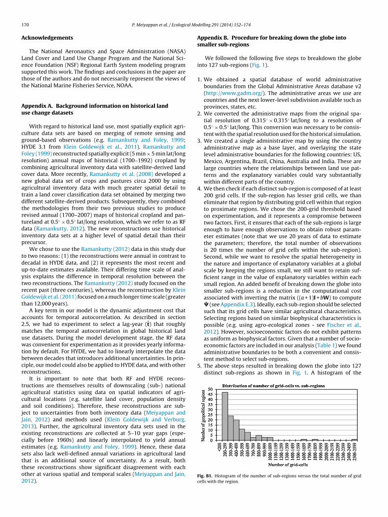
1 al Mo
A
Lestt
Au
cgHFrccnatdtrtdip
tduytrGt
a2muwtbcr
tacajJ2ecestto2
administrative boundaries to be both a convenient and consis-tent method to select sub-regions.
5. The above steps resulted in breaking down the globe into 127distinct sub-regions as shown in Fig. 1. A histogram of the
70 P. Meiyappan et al. / Ecologic
cknowledgements
The National Aeronautics and Space Administration (NASA)and Cover and Land Use Change Program and the National Sci-nce Foundation (NSF) Regional Earth System modeling programupported this work. The findings and conclusions in the paper arehose of the authors and do not necessarily represent the views ofhe National Marine Fisheries Service, NOAA.
ppendix A. Background information on historical landse change datasets
With regard to historical land use, most spatially explicit agri-ulture data sets are based on merging of remote sensing andround-based observations (e.g. Ramankutty and Foley, 1999;YDE 3.1 from Klein Goldewijk et al., 2011). Ramankutty andoley (1999) reconstructed spatially explicit (5 min × 5 min lat/longesolution) annual maps of historical (1700–1992) cropland byombining agricultural inventory data with satellite-derived landover data. More recently, Ramankutty et al. (2008) developed aew global data set of crops and pastures circa 2000 by usinggricultural inventory data with much greater spatial detail torain a land cover classification data set obtained by merging twoifferent satellite-derived products. Subsequently, they combinedhe methodologies from their two previous studies to produceevised annual (1700–2007) maps of historical cropland and pas-ureland at 0.5◦ × 0.5◦ lat/long resolution, which we refer to as RFata (Ramankutty, 2012). The new reconstructions use historical
nventory data sets at a higher level of spatial detail than theirrecursor.
We chose to use the Ramankutty (2012) data in this study dueo two reasons: (1) the reconstructions were annual in contrast toecadal in HYDE data, and (2) it represents the most recent andp-to-date estimates available. Their differing time scale of anal-sis explains the difference in temporal resolution between thewo reconstructions. The Ramankutty (2012) study focused on theecent past (three centuries), whereas the reconstruction by Kleinoldewijk et al. (2011) focused on a much longer time scale (greater
han 12,000 years).A key term in our model is the dynamic adjustment cost that
ccounts for temporal autocorrelation. As described in section.5, we had to experiment to select a lag-year (t) that roughlyatches the temporal autocorrelation in global historical land
se datasets. During the model development stage, the RF dataas convenient for experimentation as it provides yearly informa-
ion by default. For HYDE, we had to linearly interpolate the dataetween decades that introduces additional uncertainties. In prin-iple, our model could also be applied to HYDE data, and with othereconstructions.
It is important to note that both RF and HYDE recons-ructions are themselves results of downscaling (sub-) nationalgricultural statistics using data on spatial indicators of agri-ultural locations (e.g. satellite land cover, population densitynd soil conditions). Therefore, these reconstructions are sub-ect to uncertainties from both inventory data (Meiyappan andain, 2012) and methods used (Klein Goldewijk and Verburg,013). Further, the agricultural inventory data sets used in thexisting reconstructions are collected at 5–10 year gaps (espe-ially before 1960s) and linearly interpolated to yield annualstimates (e.g. Ramankutty and Foley, 1999). Hence, these data
ets also lack well-defined annual variations in agricultural landhat is an additional source of uncertainty. As a result, bothhese reconstructions show significant disagreement with eachther at various spatial and temporal scales (Meiyappan and Jain,012).delling 291 (2014) 152–174
Appendix B. Procedure for breaking down the globe intosmaller sub-regions
We followed the following five steps to breakdown the globeinto 127 sub-regions (Fig. 1).
1. We obtained a spatial database of world administrativeboundaries from the Global Administrative Areas database v2(http://www.gadm.org/). The administrative areas we use arecountries and the next lower-level subdivision available such asprovinces, states, etc.
2. We converted the administrative maps from the original spa-tial resolution of 0.315◦ × 0.315◦ lat/long to a resolution of0.5◦ × 0.5◦ lat/long. This conversion was necessary to be consis-tent with the spatial resolution used for the historical simulation.
3. We created a single administrative map by using the countryadministrative map as a base layer, and overlaying the statelevel administrative boundaries for the following countries: US,Mexico, Argentina, Brazil, China, Australia and India. These arelarge countries where the relationships between land use pat-terns and the explanatory variables could vary substantiallywithin different parts of the country.
4. We then check if each distinct sub-region is composed of at least200 grid cells. If the sub-region has lesser grid cells, we thaneliminate that region by distributing grid cell within that regionto proximate regions. We chose the 200-grid threshold basedon experimentation, and it represents a compromise betweentwo factors. First, it ensures that each of the sub-regions is largeenough to have enough observations to obtain robust param-eter estimates (note that we use 20 years of data to estimatethe parameters; therefore, the total number of observationsis 20 times the number of grid cells within the sub-region).Second, while we want to resolve the spatial heterogeneity inthe nature and importance of explanatory variables at a globalscale by keeping the regions small, we still want to retain suf-ficient range in the value of explanatory variables within eachsmall region. An added benefit of breaking down the globe intosmaller sub-regions is a reduction in the computational costassociated with inverting the matrix ((a + 1)I + bW) to compute� (see Appendix E.3). Ideally, each sub-region should be selectedsuch that its grid cells have similar agricultural characteristics.Selecting regions based on similar biophysical characteristics ispossible (e.g. using agro-ecological zones - see Fischer et al.,2012). However, socioeconomic factors do not exhibit patternsas uniform as biophysical factors. Given that a number of socio-economic factors are included in our analysis (Table 1) we found
Fig. B1. Histogram of the number of sub-regions versus the total number of gridcells with the region.
al Mo
Am
se(meiattr
C
fm(mfplsoetsoiis
l(iaKp2tas
C
aBdd(gwnlcwteui
P. Meiyappan et al. / Ecologic
number of sub-regions versus the total number of grid cellswithin the region is shown in Fig. B1.
ppendix C. Explanatory variables for land use allocationodel
Table 1 lists the 46 explanatory variables used in our regres-ion analysis. Table 2 lists the source data used to compile thexplanatory factors for model evaluation. Table 2 also includesas footnotes) information on processing of raw data sources to
atch the spatial and temporal resolution required for our modelvaluation. Here we provide details on: (1) the rationale for select-ng these explanatory factors, and (2) any additional refinementspplied to the raw data to construct the explanatory variables. Allhe 46 explanatory variables compiled for model evaluation coverhe time period 1900-2005 (annual time steps) at a uniform spatialesolution of 0.5◦ × 0.5◦ lat/long.
.1. Climate
To determine the climate suitability to cropland and pasturelandor each year, we use seasonal (spring, summer, fall and winter)
ean temperature, precipitation, and potential evapotranspirationPET) for the 3 preceding years to allow for adaptive land use adjust-
ents. Inclusion of time-lagged climate variables as explanatoryactors is motivated by the fact that climatic conditions over theast few years are taken into account to evaluate the potential
and suitability for agriculture, prior to making investment deci-ions (Mu et al., 2013). In other words, land use decisions are basedn expected climate rather than current weather conditions. Thisffect is not implicitly reflected in our dynamic cost adjustmenterm (first term in Eq. (12)) for two reasons. First, the potential landuitability for the current year is evaluated independent of previ-us land use patterns. Second, the dynamic cost adjustment termncludes a ten-year time-lag effect, whereas land use adjustmentsn response to climate change occur over a relatively smaller timecale (Mu et al., 2013).
According to agronomic studies, plant growth is partly a non-inear function of weather conditions, especially temperatureSchlenker and Roberts, 2006). To account for non-linearity, we alsonclude squared terms for each of the three seasonal climate vari-bles as explanatory factors in our analysis. We use temperature inelvins to avoid squaring of negative terms. While historical tem-erature and precipitation data were measured values (Harris et al.,013), PET is estimated using the grass reference evapotranspira-ion method (Ekström et al., 2007). PET indicates the capacity of thetmosphere to remove water from the surface through processesuch as winds and radiative energy transfer.
.2. Climate variability
Given the significant evidence on the impacts of climate vari-bility on land use decisions (e.g. Parry et al., 1999; Olesen andindi, 2002), we use three indices reflective of climate variability:rought, temperature, and precipitation extremes. For incidence ofrought, we use the seasonal Palmer Drought Severity Index (PDSI)Dai, 2011a,b). PDSI is a measurement of dryness with values ran-ing between -10 (dry) and +10 (wet). For temperature extremes,e use the heat wave duration index, calculated by counting theumber of days in a year with maximum temperature higher by at
east 5 ◦C than the climatological norm (1961–1990) for the samealendar day (Alexander et al., 2006). For precipitation extremes,e use the simple daily intensity index defined as the annual
otal precipitation divided by the number of wet days (Alexandert al., 2006). Both the temperature and precipitation extreme indexsed here are qualitatively representative of other indices measur-
ng temperature and precipitation extremes, respectively (Tebaldi
delling 291 (2014) 152–174 171
et al., 2006). Similar indices representative of climate extremeswere used by Mu et al. (2013) to understand the impacts of climateadaptation on the US land use trends.
Pastureland extent and livestock comfort are correlated.Temperature-humidity index (THI) is an indicator of the degree ofdiscomfort experienced by cattle due to seasonal conditions. Previ-ous studies have shown that higher THI in summer results in lowerfeed intake of livestock, thus inducing a smaller number of animalsper hectare, and a heavier stocking rate in the spring or winter(Hubbard et al., 1999; Mu et al., 2013). We estimated seasonal THIfollowing Mu et al. (2013).
The PDSI data was at 2.5◦ × 2.5◦ lat/long resolution which welinearly interpolated to 0.5◦ × 0.5◦ lat/long (Table 2). This adjust-ment will affect the allocation patterns, and we did not conduct asystematic sensitivity analysis to test the results against differentinterpolation techniques. In general, the interpolation techniquefor an explanatory variable should be given more focus, if that vari-able is sensitive in determining the allocation patterns (i.e. its ‘ˇ’value estimated from Eq. (23) is non-zero and significant).
C.3. Soil and terrain characteristics
We use five different factors indicating soil suitability for agri-culture (Table 1) as explanatory variables in our analysis. Each 5 mingrid cell in the original data was classified into one of the sevencategories, each indicating a different percentage range of soil suit-ability (Table 2). For each category, we take the median suitabilitypercentage and aggregate the data to 0.5◦ × 0.5◦ lat/long resolutionby area-weighted averaging. We process the map for terrain con-straints similarly to the aggregation procedure followed for soilconstraints.
We assume that soil and terrain conditions do not change withinthe time frame of analysis (∼100 years), because soil developmentprocesses are very slow. However, this assumption might not holdin regions where organic content could build up rapidly. More-over, consistent and temporally varying global maps of soil andterrain condition are unavailable historically and are unlikely to besimulated by Earth System Models for future projections.
C.4. Urban area and population
We include urban land and urban and rural population densityvariables as potential explanatory factors because these are con-sidered important drivers of land use change (Geist et al., 2006). Inaddition to population density, we also include four-year averagedrates of change in urban and rural population density to account forthe impact of changes in population pressure on land use allocationpatterns.
C.5. Market influence index
Markets play a prominent role in shaping agriculture, defor-estation, and other land use patterns (Lambin et al., 2001; Lambinand Meyfroidt, 2011). However, global scale studies have largelyignored the influence of markets in shaping land use patterns dueprimarily to lack of global scale data on markets. Here, we describeour approach to derive a single variable called market influenceindex to use as an explanatory variable in the allocation proce-dure. The market influence index is a combination of two variables:market accessibility and market importance.
Verburg et al. (2011) developed the first high-resolution (1 km2)global map (for 2005) indicating accessibility to markets. In simpleterms, their market accessibility index reflects the travel time to
nearest cities, taking into account travel impedance due to sev-eral terrain characteristics (e.g. road networks). The index variesfrom 0 (low accessibility) to 1 (high accessibility). For our analysis,we require market accessibility maps for the entire 20th century,
1 al Mo
w(tfbiihtisbto
A
wupcpumopWZawa
A
eoscetfa(stwvmpmo
ctsro1wbattom
72 P. Meiyappan et al. / Ecologic
hereas a number of terrain characteristics used by Verburg et al.2011) (e.g. road networks, wetlands) were unavailable globally forhe historical period and are also unlikely to be simulated by IAMsor the future. Instead, we model the market accessibility index toe a function of urban land area alone, neglecting other measures of
nfrastructural development. The rationale behind our assumptions that a grid cell with a higher fraction of urban area would likelyave more accessibility (e.g. road networks and other infrastruc-ure) as well. A reciprocal function is commonly used in spatialnteraction and gravity models to manipulate distance or acces-ibility. We follow a similar approach and model the relationshipetween the year 2005 urban land area (Goldewijk et al., 2010) andhe corresponding market accessibility index (Verburg et al., 2011)f the form:
g = c1b−c2g
here ‘Ag’ is the market accessibility index in grid cell ‘g’, ‘bg’ is therban land fraction specific to each grid cell, and ‘c1’ and ‘c2’ are thearameters to be estimated. We fit the model separately for eachontinent. We assume the same relationships to be true at any otheroint of time and we combine them with historical (1900–2005)rban land data (Goldewijk et al., 2010) to produce annual maps ofarket accessibility. One can think of market influence as reflective
f both market importance and its accessibility. Gross Domesticroduct (GDP) is a well-accepted measure of market importance.e multiplied the national per capita GDP values (Bolt and van
anden, 2013) with spatially explicit market access data to produce data set of market influence for the period 1900-2005. In otherords, we downscale GDP per capita to grid cells using the market
ccessibility index.
ppendix D. On multicollinearity and excess zeros
Multicollinearity is a common problem in land use change mod-ling where one or more explanatory variables are dependentn each other. A high degree of multicollinearity results in hightandard errors and spurious parameter estimates. We used a prioriorrelation analysis and did not find any pair of the 46 standardizedxplanatory variables that exceeded a correlation of 0.7 for each ofhe 127 sub-regions. We therefore did not discard any explanatoryactor from our model. For comparison, a correlation of 0.8 is used as
threshold in land-change studies to discard explanatory variablesLesschen et al., 2005). Even in the presence of multicollinearity, thepecification of error terms in our estimation procedure implieshat our point estimates are unbiased. Further, multicollinearityill not affect the efficiency of the fitted model to new data pro-
ided that the explanatory variables follow the same pattern ofulticollinearity in the new data as in the data based on which the
arameters were estimated. A problem would occur only if two orore explanatory variables are a perfect linear combination of each
ther.There are three approaches commonly followed in land use
hange models to eliminate explanatory variables due to mul-icollinearity: a priori correlation analysis, factor analysis andtepwise regression (Lesschen et al., 2005). All of them have a highisk of throwing out important explanatory variables and causingmitted variable bias, among many others (James and McCulloch,990). These methods are viable if used for smaller scale studies,here additional care can be taken on the explanatory variables
eing eliminated from the model. However, this task is taxing at global scale. Additionally, given the limited number of explana-
ory factors available for global scale analysis, it is crucial to utilizehem to the maximum potential possible. In the initial stages ofur model development, we experimented with a state-of-the-artethod to deal with multicollinearity, elastic-net regularizationdelling 291 (2014) 152–174
(Zou and Hastie, 2005). We found the elastic-net method to bemore effective than the traditional approaches used in land usechange models. The elastic-net method tries to capitalize on thestrengths of correlated variables by converging their coefficientstowards each other rather than eliminating them. Unfortunately,we could not build elastic-net regularization into our final esti-mation procedure because the current packages (Friedman et al.,2007, 2010) available for elastic-net cannot accommodate nonlin-ear restrictions among coefficients.
As evident from the historical land use patterns (Figs. 3–8), thereare many locations around the world that are unsuitable for agri-culture (i.e.) grid cells where cropland and pastureland areas arezero consistently. When estimating Eq. (23), having excessive zero-valued observation could result in biased parameter estimates. Thisis known as the excess-zeros problem (Breen, 1996). To determinewhether there is bias in our estimates, we estimated Eq. (23) witha “trimmed” sample where the grid cells unsuitable for agricul-ture were removed (see censored regressions – Breen, 1996). Wethen compared the estimated parameters for each of the 127 sub-regions with those obtained without “trimming” the sample. Withthe exception of four regions, we found no significant problem withexcess-zeros. Within these four regions (e.g. Alaska), more than 95%of the total grid cells had zero land use areas for the entire 20thcentury. For the grid cells within these four regions, we force themodel not to allocate any cropland and pastureland through Eq. (9)by replacing one on the right-hand side of the equation with zero.If excess-zeros had been a problem in some regions of the globe,then maximum likelihood estimation with a censored regressionmodel is a consistent estimation method (Breen, 1996).
Appendix E. Supplementary data
Supplementary data associated with this article can be found,in the online version, at http://dx.doi.org/10.1016/j.ecolmodel.2014.07.027.
References
Agarwal, C., Green, G.M., Grove, J.M., Evans, T.P., Schweik, C.M., 2002. A Review andAssessment of Land Use Change Models: Dynamics of Space, Time, and HumanChoice. US Department of Agriculture, Forest Service, Northeastern ResearchStation, Newton Square, PA, pp. 12–27.
Alexander, L.V., Zhang, X., Peterson, T.C., Caesar, J., Gleason, B., Klein Tank, A.M.G.,Vazquez-Aguirre, J.L., 2006. Global observed changes in daily climate extremesof temperature and precipitation. J. Geophys. Res. Atmos. (1984–2012) 111 (D5).
Alkemade, R., van Oorschot, M., Miles, L., Nellemann, C., Bakkenes, M., ten Brink, B.,2009. GLOBIO3: a framework to investigate options for reducing global terres-trial biodiversity loss. Ecosystems 12 (3), 374–390.
Augustin, N.H., Mugglestone, M.A., Buckland, S.T., 1996. An autologistic model forthe spatial distribution of wildlife. J. Appl. Ecol., 339–347.
Bennett, E.M., Carpenter, S.R., Caraco, N.F., 2001. Human impact on erodable phos-phorus and eutrophication: a global perspective. BioScience 51 (3), 227–234.
Bolt, J., van Zanden, J.L., 2013. The Maddison Project: The First Update of theMaddison project; Re-Estimating Growth Before 1820. Maddison-Project Work-ing Paper WP-4, Available from http://www.ggdc.net/maddison/maddison-project/home.htm
Bouwman, A.F., Kram, T., Klein Goldewijk, K., 2006. Integrated Modeling of GlobalEnvironmental Change. An overview of IMAGE 2.4. Netherlands EnvironmentalAssessment Agency, Bilthoven.
Breen, B., 1996. Regression Models: Censored, Sample Selected or Truncated Data.Sage Publications, London/Thousand Oaks, CA.
Briassoulis, H., 2000. Analysis of land use change: theoretical and modelingapproaches. In: Loveridge, S. (Ed.), The Web Book of Regional Science. WestVirginia University, Morgantown.
Bruinsma, J., 2009. The resource outlook to 2050: by how much do land, waterand crop yields need to increase by 2050? In: How to feed the World in 2050.Proceedings of a Technical Meeting of Experts, Rome, Italy, 24–26 June 2009.Food and Agriculture Organization of the United Nations (FAO), pp. 1–33.
Dai, A., 2011a. Characteristics and trends in various forms of the Palmer DroughtSeverity Index during 1900–2008. J. Geophys. Res. Atmos. (1984–2012) 116(D12.).
Dai, A., 2011b. Drought under global warming: a review. Wiley Interdiscip. Rev.Climate Change 2 (1), 45–65.
al Mo
D
E
E
F
F
F
F
F
F
G
G
G
G
G
H
H
H
H
H
H
H
H
H
I
J
J
K
K
K
P. Meiyappan et al. / Ecologic
ormann, C., M McPherson, J., B Araújo, M., Bivand, R., Bolliger, J., Carl, G., Wilson, R.,2007. Methods to account for spatial autocorrelation in the analysis of speciesdistributional data: a review. Ecography 30 (5), 609–628.
kström, M., Jones, P.D., Fowler, H.J., Lenderink, G., Buishand, T.A., Conway, D., 2007.Regional climate model data used within the SWURVE project – 1: projectedchanges in seasonal patterns and estimation of PET. Hydrol. Earth Syst. Sci. 11(3), 1069–1083.
rb, K.H., Haberl, H., Jepsen, M.R., Kuemmerle, T., Lindner, M., Müller, D., Ver-burg, P.H., Reenberg, A., 2013. A conceptual framework for analysing andmeasuring land use intensity. Curr. Opin. Environ. Sust., http://dx.doi.org/10.1016/j.cosust.2013.07.010.
ischer, G., Nachtergaele, F.O., Prieler, S., Teixeira, E., Tóth, G., van Velthuizen, H.,Wiberg, D., 2012. Global Agro-Ecological Zones (GAEZ v3. 0): Model Documen-tation. International Institute for Applied systems Analysis (IIASA), Laxenburg.Austria and the Food and Agriculture Organization of the United Nations (FAO),Rome, Italy, Data accessible from http://www.fao.org/nr/gaez/en/
oley, J.A., DeFries, R., Asner, G.P., Barford, C., Bonan, G., Carpenter, S.R., Snyder, P.K.,2005. Global consequences of land use. Science 309 (5734), 570–574.
oley, J.A., Ramankutty, N., Brauman, K.A., Cassidy, E.S., Gerber, J.S., Johnston, M.,Zaks, D.P., 2011. Solutions for a cultivated planet. Nature 478 (7369), 337–342.
riedman, J., Hastie, T., Höfling, H., Tibshirani, R., 2007. Pathwise coordinate opti-mization. Ann. Appl. Stat. 1 (2), 302–332.
riedman, J., Hastie, T., Tibshirani, R., 2010. Regularization paths for generalizedlinear models via coordinate descent. J. Stat. Softw. 33 (1), 1.
uchs, R., Herold, M., Verburg, P., Clevers, J., Eberle, J., 2014. Gross changes in recons-tructions of historic land use for Europe during the 20th century. Global ChangeBiol. (in review).
eist, H.J., McConnell, W.J., Lambin, E.F., Moran, E., Alves, D., Rudel, T.K., 2006.Causes and trajectories of land use/cover change. In: Lambin, E.F., Geist HJ (Eds.),Land Use and Land-Cover Change. Local Processes and Global Impacts. Springer-Verlag, Berlin Heidelberg, pp. 41–70.
oldewijk, K.K., Beusen, A., Janssen, P., 2010. Long-term dynamic modeling of globalpopulation and built-up area in a spatially explicit way: HYDE 3.1. Holocene 20(4), 565–573.
olub, A., Hertel, T., Sohngen, B., 2008. Land Use Modeling in Recursively-dynamicGTAP Framework (No. 2609). GTAP Working paper No. 48. Center for GlobalTrade Analysis, Department of Agricultural Economics, Purdue University.
ouel, C., Hertel, T.W., 2006. Introducing Forest Access Cost Functions into a GeneralEquilibrium Model. GTAP Research Memorandum 8.
reen, R.E., Cornell, S.J., Scharlemann, J.P., Balmford, A., 2005. Farming and the fateof wild nature. Science 307 (5709), 550–555.
allgren, W., Schlosser, C.A., Monier, E., Kicklighter, D., Sokolov, A., Melillo, J., 2013.Climate impacts of a large-scale biofuels expansion. Geophys. Res. Lett. 40 (8),1624–1630.
arris, I., Jones, P.D., Osborn, T.J., Lister, D.H., 2013. Updated high-resolutiongrids of monthly climatic observations. Int. J. Climatol., http://dx.doi.org/10.1002/joc.3711.
avlik, P., Schneider, U.A., Schmid, E., Böttcher, H., Fritz, S., Skalsky, R., Obersteiner,M., 2011. Global land use implications of first and second generation biofueltargets. Energy Policy 39 (10), 5690–5702.
eistermann, M., Müller, C., Ronneberger, K., 2006. Land in sight? Achievements,deficits and potentials of continental to global scale land use modeling. Agric.Ecosyst. Environ. 114 (2), 141–158.
ibbard, K., Janetos, A., van Vuuren, D.P., Pongratz, J., Rose, S.K., Betts, R., Fed-dema, J.J., 2010. Research priorities in land use and land-cover change for theEarth system and integrated assessment modelling. Int. J. Climatol. 30 (13),2118–2128.
oughton, R.A., 2008. Carbon flux to the atmosphere from land use changes:1850–2005. In: TRENDS: A Compendium of Data on Global Change. Car-bon Dioxide Information Analysis Center, Oak Ridge National Laboratory, U.S.Department of Energy, Oak Ridge, TN, USA.
ubbard, K.G., Stooksbury, D.E., Hahn, G.L., Mader, T.L., 1999. A climatologi-cal perspective on feedlot cattle performance and mortality related to thetemperature-humidity index. J. Prod. Agric. 12 (4), 650–653.
unter, J.E., Hamilton, M.A., 2002. The advantages of using standardized scores incausal analysis. Hum. Commun. Res. 28 (4), 552–561.
urtt, G.C., Chini, L.P., Frolking, S., Betts, R.A., Feddema, J., Fischer, G., Wang, Y.P.,2011. Harmonization of land use scenarios for the period 1500–2100: 600 yearsof global gridded annual land use transitions, wood harvest, and resulting sec-ondary lands. Climatic Change 109 (1–2), 117–161.
rwin, E.G., Geoghegan, J., 2001. Theory, data, methods: developing spatiallyexplicit economic models of land use change. Agric. Ecosyst. Environ. 85 (1),7–24.
ain, A.K., Meiyappan, P., Song, Y., House, J.I., 2013. CO2 emissions from land-usechange affected more by nitrogen cycle, than by the choice of land cover data.Global Change Biol. 19, 2893–2906.
ames, F.C., McCulloch, C.E., 1990. Multivariate analysis in ecology and systematics:panacea or Pandora’s box? Ann. Rev. Ecol. Syst. 21, 129–166.
eys, E., McConnell, W.J., 2005. Global change and the intensification of agriculturein the tropics. Global Environ. Change 15 (4), 320–337.
indermann, G., Obersteiner, M., Sohngen, B., Sathaye, J., Andrasko, K., Rametsteiner,
E., Beach, R., 2008. Global cost estimates of reducing carbon emissions throughavoided deforestation. Proc. Natl. Acad. Sci. U.S.A. 105 (30), 10302–10307.lein Goldewijk, K., Verburg, P.H., 2013. Uncertainties in global-scale reconstruct-ions of historical land use: an illustration using the HYDE data set. Landsc. Ecol.28 (5), 861–877.
delling 291 (2014) 152–174 173
Klein Goldewijk, K., Beusen, A., Van Drecht, G., De Vos, M., 2011. The HYDE 3.1 spa-tially explicit database of human-induced global land-use change over the past12,000 years. Global Ecol. Biogeogr. 20 (1), 73–86.
Kuemmerle, T., Erb, K., Meyfroidt, P., Müller, D., Verburg, P.H., Estel, S., Haberl,H., Hostert, P., Jepsen, M.R., Kastner, T., Levers, C., Lindner, M., Plutzar, C.,Verkerk, P.J., van der Zanden, E.H., Reenberg, A., 2013. Challenges and oppor-tunities in mapping land use intensity globally. Curr. Opin. Environ. Sustain. 5,484–493.
Lambin, E.F., Meyfroidt, P., 2011. Global land use change, economic globaliza-tion, and the looming land scarcity. Proc. Natl. Acad. Sci. U.S.A. 108 (9),3465–3472.
Lambin, E.F., Rounsevell, M.D.A., Geist, H.J., 2000. Are agricultural land use modelsable to predict changes in land use intensity? Agric. Ecosyst. Environ. 82 (1),321–331.
Lambin, E.F., Turner, B.L., Geist, H.J., Agbola, S.B., Angelsen, A., Bruce, J.W., Xu, J., 2001.The causes of land use and land-cover change: moving beyond the myths. GlobalEnviron. Change 11 (4), 261–269.
Lambin, E.F., Geist, H.J., Lepers, E., 2003. Dynamics of land use and land-cover changein tropical regions. Ann. Rev. Environ. Resour. 28 (1), 205–241.
Lancaster, T., 2000. The incidental parameter problem since 1948. J. Econometrics95 (2), 391–413.
Lawrence, P.J., Feddema, J.J., Bonan, G.B., Meehl, G.A., O’Neill, B.C., Oleson, K.W.,Thornton, P.E., 2012. Simulating the biogeochemical and biogeophysical impactsof transient land cover change and wood harvest in the community climatesystem model (CCSM4) from 1850 to 2100. J. Clim. 25 (9.).
Le Quéré, C., Peters, G.P., Andres, R.J., Andrew, R.M., Boden, T.A., Ciais, P., Zaehle, S.,2014. Global carbon budget 2013. Earth Syst. Sci. Data 6 (1), 235–263.
Lesschen, J.P., Verburg, P.H., Staal, S.J., 2005. Statistical Methods for Analysing theSpatial Dimension of Changes in Land Use and Farming Systems. InternationalLivestock Research Institute.
Letourneau, A., Verburg, P.H., Stehfest, E., 2012. A land use systems approach torepresent land use dynamics at continental and global scales. Environ. Model.Softw. 33, 61–79.
Lotze-Campen, H., Popp, A., Beringer, T., Müller, C., Bondeau, A., Rost, S., Lucht, W.,2010. Scenarios of global bioenergy production: the trade-offs between agricul-tural expansion, intensification and trade. Ecol. Model. 221 (18), 2188–2196.
Lubowski, R.N., Plantinga, A.J., Stavins, R.N., 2008. What drives land use change inthe United States? A national analysis of landowner decisions. Land Econ. 84 (4),529–550.
MEA, 2005. Ecosystems and Human Well-being, vol. 5. Island Press, Washington,DC.
Meiyappan, P., Jain, A.K., 2012. Three distinct global estimates of historical land-cover change and land use conversions for over 200 years. Front. Earth Sci. 6 (2),122–139.
Melillo, J.M., Reilly, J.M., Kicklighter, D.W., Gurgel, A.C., Cronin, T.W., Paltsev, S.,Schlosser, C.A., 2009. Indirect emissions from biofuels: how important? Science326 (5958), 1397–1399.
Mertens, K.C., Verbeke, L.P.C., Ducheyne, E.I., De Wulf, R.R., 2003. Using geneticalgorithms in sub-pixel mapping. Int. J. Remote Sens. 24 (21), 4241–4247.
Meyfroidt, P., 2013. Environmental cognitions, land change, and social–ecologicalfeedbacks: an overview. J. Land Use Sci. 8 (3), 314–367.
Meyfroidt, P., Lambin, E.F., Erb, K.H., Hertel, T.W., 2013. Globalization of land use:distant drivers of land change and geographic displacement of land use. Curr.Opin. Environ. Sustain. 5 (5), 438–444.
Moss, R.H., Edmonds, J.A., Hibbard, K.A., Manning, M.R., Rose, S.K., van Vuuren,D.P., Wilbanks, T.J., 2010. The next generation of scenarios for climate changeresearch and assessment. Nature 463 (7282), 747–756.
Mu, J.E., McCarl, B.A., Wein, A.M., 2013. Adaptation to climate change: changes infarmland use and stocking rate in the U.S. Mitigation Adapt. Strat. Global Change18 (6.), http://dx.doi.org/10.1007/s11027-012-9384-4.
NRC, 2014. Advancing Land Change Modeling: Opportunities and Research Require-ments. National Academy Press, Washington, DC.
O’Neill, B., Verburg, P., 2012. Spatial land use modeling: simulating decisions andtheir consequences for climate, carbon, and water, Global Land Project (GLP)News Letter, Issue No 9.
OECD, 2012. OECD Environmental Outlook to 2050: The Consequences of Inaction.Organisation for Economic Co-operation Development, Paris, http://dx.doi.org/10.1787/9789264122246-en.
Olesen, J.E., Bindi, M., 2002. Consequences of climate change for European agricul-tural productivity, land use and policy. Eur. J. Agron. 16 (4), 239–262.
O’Neill, B.C., Dalton, M., Fuchs, R., Jiang, L., Pachauri, S., Zigova, K., 2010. Global demo-graphic trends and future carbon emissions. Proc. Natl. Acad. Sci. U.S.A. 107 (41),17521–17526.
Overmars, K.P., De Koning, G.H.J., Veldkamp, A., 2003. Spatial autocorrelation inmulti-scale land use models. Ecol. Model. 164 (2), 257–270.
Parker, D.C., Manson, S.M., Janssen, M.A., Hoffmann, M.J., Deadman, P., 2003. Multi-agent systems for the simulation of land use and land-cover change: a review.Ann. Assoc. Am. Geogr. 93 (2), 314–337.
Parry, M., Rosenzweig, C., Iglesias, A., Fischer, G., Livermore, M., 1999. Climate changeand world food security: a new assessment. Global Environ. Change 9, S51–S67.
Pereira, H.M., Leadley, P.W., Proenc a, V., Alkemade, R., Scharlemann, J.P., Fernandez-
Manjarrés, J.F., Walpole, M., 2010. Scenarios for global biodiversity in the 21stcentury. Science 330 (6010), 1496–1501.Phalan, B., Onial, M., Balmford, A., Green, R.E., 2011. Reconciling food production andbiodiversity conservation: land sharing and land sparing compared. Science 333(6047), 1289–1291.
1 al Mo
P
P
P
R
R
R
R
R
R
R
R
R
R
R
S
S
S
S
S
74 P. Meiyappan et al. / Ecologic
ielke, R.A., Pitman, A., Niyogi, D., Mahmood, R., McAlpine, C., Hossain, F., de Noblet,N., 2011. Land use/land cover changes and climate: modeling analysis and obser-vational evidence. Wiley Interdiscip. Rev. Climate Change 2 (6), 828–850.
itman, A.J., de Noblet-Ducoudré, N., Cruz, F.T., Davin, E.L., Bonan, G.B., Brovkin, V.,Voldoire, A., 2009. Uncertainties in climate responses to past land cover change:first results from the LUCID intercomparison study. Geophys. Res. Lett. 36 (14).
ortmann, F.T., Siebert, S., Döll, P., 2010. MIRCA2000—global monthly irrigated andrainfed crop areas around the year 2000: a new high-resolution data set foragricultural and hydrological modeling. Global Biogeochem. Cycles 24 (1).
amankutty, N., 2012. Global Cropland and Pasture Data from 1700–2007, Availableonline at [http://www.geog.mcgill.ca/∼nramankutty/Datasets/Datasets.html]from the LUGE (Land Use and the Global Environment) Laboratory, Depart-ment of Geography, McGill University, Montreal, Quebec, Canada (accessed on25.09.12).
amankutty, N., Foley, J.A., 1999. Estimating historical changes in global land cover:Croplands from 1700 to 1992. Global Biogeochem. Cycles 13 (4), 997–1027.
amankutty, N., Foley, J.A., Norman, J., McSweeney, K., 2002. The global distributionof cultivable lands: current patterns and sensitivity to possible climate change.Global Ecol. Biogeogr. 11 (5), 377–392.
amankutty, N., Evan, A.T., Monfreda, C., Foley, J.A., 2008. Farming the planet: 1.Geographic distribution of global agricultural lands in the year 2000. GlobalBiogeochem. Cycles 22 (1.).
ay, D.K., Ramankutty, N., Mueller, N.D., West, P.C., Foley, J.A., 2012. Recent patternsof crop yield growth and stagnation. Nat. Commun. 3, 1293.
eilly, J., Melillo, J., Cai, Y., Kicklighter, D., Gurgel, A., Paltsev, S., Schlosser, A., 2012.Using land to mitigate climate change: hitting the target, recognizing the trade-offs. Environ. Sci. Technol. 46 (11), 5672–5679.
okityanskiy, D., Benítez, P.C., Kraxner, F., McCallum, I., Obersteiner, M., Ramet-steiner, E., Yamagata, Y., 2007. Geographically explicit global modeling of landuse change, carbon sequestration, and biomass supply. Technol. Forecast. Soc.Change 74 (7), 1057–1082.
onneberger, K., Tol, R.S.J., Schneider, U.A., 2005. KLUM: A Simple Model of GlobalAgricultural Land use a Coupling Tool of Economy and Vegetation. WorkingPaper FNU-65. Hamburg University, Hamburg, Germany.
onneberger, K., Berrittella, M., Bosello, F., Tol, R.S., 2009. KLUM@ GTAP: introducingbiophysical aspects of land use decisions into a computable general equilibriummodel a coupling experiment. Environ. Model. Assess. 14 (2), 149–168.
ounsevell, M.D., Arneth, A., 2011. Representing human behaviour and decisionalprocesses in land system models as an integral component of the Earth system.Global Environ. Change 21 (3), 840–843.
ounsevell, M.D.A., Arneth, A., Alexander, P., Brown, D.G., de Noblet-Ducoudré, N.,Ellis, E., Finnigan, J., Galvin, K., Grigg, N., Harman, I., Lennox, J., Magliocca, N.,Parker, D., O’Neill, B.C., Verburg, P.H., Young, O., 2014. Towards decision-basedglobal land use models for improved understanding of the Earth system. EarthSyst. Dyn. 5, 117–137, http://dx.doi.org/10.5194/esd-5-117-2014.
arofim, M.C., Reilly, J.M., 2011. Applications of integrated assessment modeling toclimate change. Wiley Interdiscip. Rev. Climate Change 2 (1), 27–44.
chaldach, R., Priess, J.A., Alcamo, J., 2011. Simulating the impact of biofuel devel-opment on country-wide land use change in India. Biomass Bioenergy 35 (6),2401–2410.
chlenker, W., Roberts, M.J., 2006. Nonlinear effects of weather on corn yields. Appl.Econ. Perspect. Policy 28 (3), 391–398.
iebert, S., Döll, P., Hoogeveen, J., Faures, J.-M., Frenken, K., Feick, S., 2005. Develop-
ment and validation of the global map of irrigation areas. Hydrol. Earth Syst. Sci.9, 535–547, http://dx.doi.org/10.5194/hess-9-535-2005.mith, P., Gregory, P.J., Van Vuuren, D., Obersteiner, M., Havlík, P., Rounsevell, M.,Bellarby, J., 2010. Competition for land. Philos. Trans. R. Soc. B: Biol. Sci. 365(1554), 2941–2957.
delling 291 (2014) 152–174
Souty, F., Brunelle, T., Dumas, P., Dorin, B., Ciais, P., Crassous, R., Bondeau, A., 2012.The Nexus Land-Use model version 1.0, an approach articulating biophysicalpotentials and economic dynamics to model competition for land-use. Geosci.Model Develop. 1, 1297–1322.
Souty, F., Dorin, B., Brunelle, T., Dumas, P., Ciais, P., 2013. Modelling economic andbiophysical drivers of agricultural land use change. Calibration and evaluationof the Nexus Land use model over 1961–2006. Geosci. Model Develop. Discuss.6 (4), 6975–7046.
Stehfest, E., Bouwman, L., van Vuuren, D.P., den Elzen, M.G., Eickhout, B., Kabat, P.,2009. Climate benefits of changing diet. Clim. Change 95 (1–2), 83–102.
Taylor, K.E., Stouffer, R.J., Meehl, G.A., 2012. An overview of CMIP5 and the experi-ment design. Bull. Am. Meteorol. Soc. 93 (4), 485–498.
Tebaldi, C., Hayhoe, K., Arblaster, J.M., Meehl, G.A., 2006. Going to the extremes.Climatic Change 79 (3-4), 185–211.
TEEB, 2010. The Economic of Ecosystems and Biodiversity: Mainstreaming theEconomics of Nature: a Synthesis of the Approach, Conclusions and Recommen-dations to the TEEB.
Thenkabail, P.S., Biradar, C.M., Noojipady, P., Dheeravath, V., Li, Y., Velpuri, M., Dutta,R., 2009. Global irrigated area map (GIAM), derived from remote sensing, for theend of the last millennium. Int. J. Remote Sens. 30 (14), 3679–3733.
Tilman, D., Balzer, C., Hill, J., Befort, B.L., 2011. Global food demand and the sus-tainable intensification of agriculture. Proc. Natl. Acad. Sci. U.S.A. 108 (50),20260–20264.
UNEP, 2012. Global Environmental Outlook: Environment for the Future We Want,GEO 5. United Nations Environmental Programme.
US Environmental Protection Agency (EPA), 2000. Projecting Land use Change: ASummary of Models for Assessing the Effects of Community Growth and Changeon Land Use Patterns. U.S. Environmental Protection Agency, Cincinnati, OH,Office of Research and Development Publication EPA/600/R-00/098.
van Asselen, S., Verburg, P.H., 2012. A Land System representation for global assess-ments and land use modeling. Global Change Biol. 18 (10), 3125–3148.
van Asselen, S., Verburg, P.H., 2013. Land cover change or land use intensification:simulating land system change with a global-scale land change model. GlobalChange Biol., http://dx.doi.org/10.1111/gcb.12331.
van Vuuren, D.P., Edmonds, J., Kainuma, M., Riahi, K., Thomson, A., Hibbard, K., Rose,S.K., 2011. The representative concentration pathways: an overview. ClimaticChange 109 (1–2), 5–31.
van Vuuren, D.P., Bayer, L.B., Chuwah, C., Ganzeveld, L., Hazeleger, W., van den Hurk,B., van Noije, T., O’Neill, B., Strengers, B.J., 2012. A comprehensive view on climatechange: coupling of Earth system and Integrated Assessment Models. Environ.Res. Lett. 7 (2), 024012.
Verburg, P.H., Schot, P.P., Dijst, M.J., Veldkamp, A., 2004. Land use change modelling:current practice and research priorities. GeoJournal 61 (4), 309–324.
Verburg, P.H., Ellis, E.C., Letourneau, A., 2011. A global assessment of market acces-sibility and market influence for global environmental change studies. Environ.Res. Lett. 6 (3), 034019.
Verburg, P.H., van Asselen, S., van der Zanden, E.H., Stehfest, E., 2013. The repre-sentation of landscapes in global scale assessments of environmental change.Landsc. Ecol., http://dx.doi.org/10.1007/s10980-012-9745-0.
Wang, X., (Ph.D. Thesis) 2008. Impacts of Greenhouse Gas Mitigation Policies on Agri-cultural Land. Massachusetts Institute of Technology, Cambridge, MA, Availableat globalchange.mit.edu/files/document/Wang PhD 08.pdf (accessed 28.07.13).
Wilkenskjeld, S., Kloster, S., Pongratz, J., Raddatz, T., Reick, C., 2014. Compar-
ing the influence of net and gross anthropogenic land use and land coverchanges on the carbon cycle in the MPI-ESM. Biogeosci. Discuss. 11 (4),5443–5469.Zou, H., Hastie, T., 2005. Regularization and variable selection via the elastic net. J.R. Stat. Soc.: Ser. B (Stat. Methodol.) 67 (2), 301–320.