spatial econometric models for evaluating rdp...

Work Package No. 4

March 2013

D4.3

Spatial econometric models for evaluating

RDP measures: analyses for the EU27

Authors: Stijn Reinhard, Vincent Linderhof, Eveline van

Leeuwen, Martijn Smit, Peter Nowicki, and Rolf Michels

Document status

Public use

Confidential use

Draft No. 1

Final

Submitted for internal review

x

x

Date

Date

29-3-2013

i

Table of contents

Tables ___________________________________________________________________ iii

Figures __________________________________________________________________ iv

Abbreviations ______________________________________________________________ v

Summary ________________________________________________________________ vi

1 Introduction ____________________________________________________________ 7

1.1 Objective of WP4.3 _______________________________________________________ 7

1.2 Using spatial econometrics for evaluating RDP measures _________________________ 8

1.3 Outline of the report _______________________________________________________ 8

2 Spatial econometrics _____________________________________________________ 9

2.1 Theory _________________________________________________________________ 9

2.2 Choice of weight matrix ___________________________________________________ 10

2.3 Empirical studies ________________________________________________________ 13

2.4 Opportunities and pitfalls __________________________________________________ 13

3 Agricultural labour productivity model ____________________________________ 15

3.1 Introduction ____________________________________________________________ 15

3.2 Theory and model _______________________________________________________ 19

3.2.1 Guide for the analysis in SPARD _________________________________________ 19

3.2.2 Model approach _______________________________________________________ 21

3.3 Data, definitions and caveats _______________________________________________ 22

3.4 Results ________________________________________________________________ 28

3.4.1 Results ______________________________________________________________ 34

3.4.2 Scenario analysis ______________________________________________________ 38

3.5 Discussion and conclusions ________________________________________________ 39

4 Environmental model ___________________________________________________ 41

4.1 Introduction ____________________________________________________________ 41

4.2 Theory and model _______________________________________________________ 44

4.2.1 Introduction __________________________________________________________ 44

4.2.2 Spillover effects _______________________________________________________ 46

4.2.3 Model _______________________________________________________________ 46


4.3.1 Impact on water quality _________________________________________________ 49

4.3.2 Impact on biodiversity __________________________________________________ 51

4.4 Results ________________________________________________________________ 56

4.4.1 Nitrogen surplus ______________________________________________________ 57

4.4.2 High Natural Value Farmland ____________________________________________ 61


5 Tourism _______________________________________________________________ 67

5.1 Introduction ____________________________________________________________ 67

5.2 Theory and model _______________________________________________________ 71

5.2.1 Introduction __________________________________________________________ 71

ii

5.2.2 Spillover effects _______________________________________________________ 72

5.2.3 Model _______________________________________________________________ 74


5.4 Results ________________________________________________________________ 77

5.4.1 Explanatory data analysis _______________________________________________ 77

5.4.2 Static specification _____________________________________________________ 78

5.4.3 Dynamic specification __________________________________________________ 81


6 Conclusions ____________________________________________________________ 86

6.1 Introduction ____________________________________________________________ 86

6.2 Did spatial analysis matter? ________________________________________________ 86

6.3 How to continue? ________________________________________________________ 88

Acknowledgement _________________________________________________________ 90

References _______________________________________________________________ 91

iii

Tables Table 3.1: Examples of investments supported under the measure ”farm modernisation“ (121). ..... 18

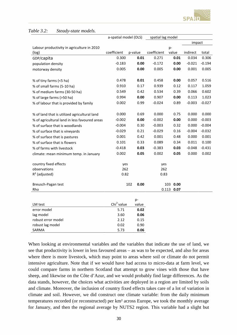
Table 3.2: Steady-state models. ......................................................................................................... 30

Table 3.3: Spatial growth models for labour productivity in agriculture in 2010 (log) ..................... 35

Table 3.4: Simplified Durbin model, split by time periods. ............................................................... 37

Table 4.1 CMEF objective-related baseline indicators for measure 214 .......................................... 43

Table 4.2 CMEF indicators for Agri-environmental measures (214) focussing on water quality and

biodiversity ....................................................................................................................... 44

Table 4.3 Moran’s I statistics for the environmental indicators (Nitrogen surplus and HNV-index )

.......................................................................................................................................... 57

Table 4.4 Static panel data model for N-surplus: a-spatial and spatial error model ......................... 58

Table 4.5 Regression results of change in N-surplus (Dynamic) panel data model and Simplified

Durbin model. ................................................................................................................... 60

Table 4.6 Static model for HNV index in 2010: a-spatial and spatial error model ........................... 63

Table 4.7 Dynamic model for HNV index: a-spatial, Durbin model and Durbin/spatial lag model 64

Table 5.1 Axis 3 EU spending on measures 311 and 313. ................................................................ 67

Table 5.2 The description of the measures 311 and 313 ................................................................... 70

Table 5.3 Hypotheses for expected spillover effects for different types of tourism at NUTS 2 areas

.......................................................................................................................................... 73

Table 5.4 Moran’s I statistics for four indicators of tourism (number of nights spent at NUTS2

level) ................................................................................................................................. 77

Table 5.5 Estimation results for log of the number of nights spent at NUTS2 level for the EU27 in

2009. ................................................................................................................................. 78

Table 5.6 Spatial error model estimation results for nights spent at NUTS2 level for the EU27 in the

period 2001-2009. ............................................................................................................. 80

Table 5.7 Estimation results for log of number of nights spent at NUTS2 level for the EU27 in the

period 2009 ....................................................................................................................... 82

Table 5.8 Results for the dynamic spatial specification of the logarithm of the number of nights

spent at NUTS2 level for the EU27 in the period 2001-2009. .......................................... 84

Table 6.1 Spatial error model estimation results for nights spent at NUTS2 level for the EU27 in the

period 2001-2009. ............................................................................................................. 87

iv

Figures Figure 2.1: Gabriel neighbours ......................................................................................................... 12

Figure 2.2: Gabriel neighbours for European NUTS2 regions ......................................................... 12

Figure 3.1: Historical development of the CAP (source: (Pack, 2011)) ........................................... 17

Figure 3.2: Intervention logic of measure 121 .................................................................................. 17

Figure 3.3: Regimes .......................................................................................................................... 24

Figure 3.4: Labour productivity in agriculture, 2000, by NUTS2 region. ........................................ 25

Figure 3.4: Labour productivity in agriculture, 2010, by NUTS2 region. ........................................ 26

Figure 3.6: Annual average spending per holding, 2000-2010, by NUTS2 region. ......................... 27

Figure 3.7: Motorway density in km of motorway per 1000 km², by NUTS2 region. ..................... 27

Figure 3.8: Country-specific levels of labour productivity, controlling for all variables in the

extensive model. ............................................................................................................. 31

Figure 3.9: Scatter plot of RDP spending (yearly average, 1999-2010) , in thousands of € and its

spatial lag ....................................................................................................................... 32

Figure 3.10: Scatter plot of labour productivity in agriculture (2010) and its spatial lag ................... 33

Figure 3.11: Scenario analysis ............................................................................................................ 39

Figure 4.1: Spending per hectare per NUTS2 region on measure 214 in 2010 ................................ 41

Figure 4.2: Objectives and indicators of measure 214 ...................................................................... 42

Figure 4.3: Scheme for the nitrogen cycle including gross nitrogen surplus .................................... 50

Figure 4.4: Nitrogen Surplus, average 2000-2004 and 2005-2008 (kg N per ha agricultural land). 51

Figure 4.5: Example of ruminant stocking density index functions, relative to different

environmental contexts. Points A-B-C-D represent respective critical stocking densities

for High Nature Value farmland .................................................................................... 54

Figure 4.6: HNV changes in the EU in the period 2000-2010 .......................................................... 56

Figure 5.1: Objectives and indicators for measure 311 (left) and 313 (right) .................................. 68

Figure 5.2: Top 10 of tourist destinations in the EU (1,000 nights spent in the country by non-

residents) ....................................................................................................................... 68

Figure 5.3: Spending per hectare (total area) on measure 311 per NUTS 2 region in 2010 ............. 69

Figure 5.4: Spending per hectare (total area) on measure 313 per NUTS 2 region in 2010 ............. 69

v

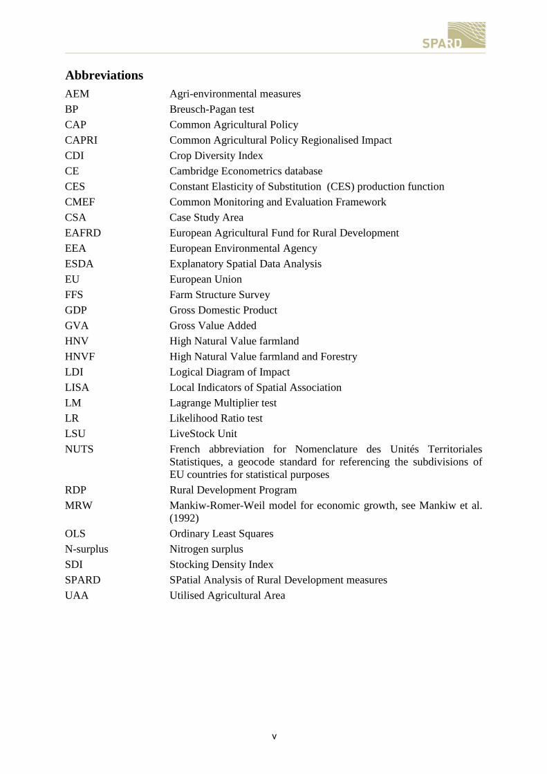
Abbreviations AEM Agri-environmental measures

BP Breusch-Pagan test

CAP Common Agricultural Policy

CAPRI Common Agricultural Policy Regionalised Impact

CDI Crop Diversity Index

CE Cambridge Econometrics database

CES Constant Elasticity of Substitution (CES) production function

CMEF Common Monitoring and Evaluation Framework

CSA Case Study Area

EAFRD European Agricultural Fund for Rural Development

EEA European Environmental Agency

ESDA Explanatory Spatial Data Analysis

EU European Union

FFS Farm Structure Survey

GDP Gross Domestic Product

GVA Gross Value Added

HNV High Natural Value farmland

HNVF High Natural Value farmland and Forestry

LDI Logical Diagram of Impact

LISA Local Indicators of Spatial Association

LM Lagrange Multiplier test LR Likelihood Ratio test

LSU LiveStock Unit

NUTS French abbreviation for Nomenclature des Unités Territoriales Statistiques, a geocode standard for referencing the subdivisions of EU countries for statistical purposes

RDP Rural Development Program

MRW Mankiw-Romer-Weil model for economic growth, see Mankiw et al. (1992)

OLS Ordinary Least Squares

N-surplus Nitrogen surplus

SDI Stocking Density Index

SPARD SPatial Analysis of Rural Development measures

UAA Utilised Agricultural Area

vi

Summary In SPARD task 4.3 EU wide spatial econometric models are identified and estimated of the. The objective of these models is to assess the impact of RDP-spending on EU objectives. The models are developed along the CMEF framework and data for ex post evaluation data of RDP are used. The model is elaborated for three measures (representing 3 axes) of the Rural Development Programme (RDP). These measure are:

• modernization of agricultural holdings (121);

• agri-environmental measures (214) and

• diversification into non-agricultural activities (311) / (313).

For all three measures, first a basic model is derived based on literature. Then data to estimate the model are gathered. It proved to be difficult to obtain the necessary data. To enable a suitable spatial econometric model, data at NUTS2 level are preferred for a longer time period to relate the development of the relevant impact indicators to the RDP-spending.

For measure 121 our model could not show a significant influence of the measure on the agricultural labour productivity (the impact indicator) at NUTS2 level. Although at a lower aggregation level (farm level) this effect can be present. Labour productivity has a clear spatial pattern, so spatial econometrics is the suitable approach.

Measure 214 consists of an array of different activities that are subsidized, so we expect that the relation between RDP spending and impact indicators is less clear. Moreover the impact indicators (e.g. biodiversity and water quality) are not measured quantitatively at NUTS2 level throughout the EU. We estimate the model using proxies for the real impact indicators (e.g. a for this study constructed proxy for High Natural Value Farmland that should reflect biodiversity).

Measure 313 objective is to stimulate tourism activities to enlarge the gross domestic product (GDP) and the reduce the share of agriculture in GDP. In the model the relation between RDP spending and nights spent by non-residents is estimated. Also in this model space matters, thus spatial econometrics is the appropriate way to estimate the model.

7

1 Introduction

1.1 Objective of WP4.3

The SPARD project aims at developing tools to analyse to what extent EU rural development measures have an impact on the economy, such as through economic growth and tourism, and at the same time contribute to the realization of environmental targets. The development of tools is based upon the Common Monitoring and Evaluation Framework (CMEF), i.e. the assessment framework of Rural Development Program measures introduced by the European Commission in consultation with the EU Member States. The CMEF distinguishes different parameters for monitoring the implementing of measures within the RDP. For each measure, CMEF prescribes the following indicators:

• baseline indicators (objective- and context-related); • input indicators (expenditures);

• output (physical); • result (physical and successful) and

• impact.

Baseline indicators describe the socio-economic, environmental and farm structure related situation of a region, while the other indicators are related to budget, implementation and impact of rural development measures. There are still many data gaps and the data delivered by the authorities in the Member States has not been sufficiently checked yet. In addition, the indicators used within the framework refer to different spatial units. Baseline indicators, for example, are available at NUTS2 level, while input, output, result and impact indicators are measured at the programming level. Input, output, and result indicators are available for the single RDP measures, while impact indicators measure the outcome of an entire program (consisting of a number of RDP measures).

In SPARD we enable policy analysis to look at causal relationships between characteristics, needs, expenditures and results of rural development measures in a spatial dimension. We analyse to what extent a spatial econometric approach will be useful to provide information on the effect of the RDP measures on impact indicators.

In WP4 of the SPARD project, Task 4.1 is the definition of the econometric test to assess the impact of RDPs. This follows from the work in WP2 to select relevant variables and the work in WP3 on the design of logical diagrams and the identification of relations that have to be tested (the identification of causal relationships). Task 4.2 proceeds with an analysis of the database for spatial patterns. This is followed by Task 4.3, which is the identification and estimation of the model at NUTS0 level. In order to prepare for the case study analyses in WP5, the next step is Task 4.4, which is the specification of the model to be used at the NUTS2 and NUTS3 levels. Task 4.5 brings together the knowledge gained in the other Tasks in WP4 through a description of a general methodology for the use of spatial econometrics in Rural Development Programmes.

8

1.2 Using spatial econometrics for evaluating RDP measures

This report describes the spatial econometric analyses framework of a selected number of RDP measures. Within SPARD, three RPD measures were preselected for the analyses at EU 27 level. For this pre-selection we have used three criteria.

1. Data availability for the impact indicators from the CMEF (see WP2), 2. The theoretical considerations from the literature on the impact indicators for the

econometric specifications models. For agricultural productivity, econometric specifications are available in the literature while there is not a clear specification for impact indicators of agri-environmental schemes and tourism.

3. The expectation of the impacts of the measures. For all axis in the RDP, one measure is selected, namely:

o modernization of agricultural holdings (121);

o agri-environment measures (214) and

o diversification into non-agricultural activities (311) or (313).

The spatial econometric analyses for the three different measures will be built upon ex-post analysis, i.e. mainly based on the input, output and result indicators provided by the RDPs themselves and the baseline indicators if available. The objective of the spatial econometric analysis is to explain the impact (based on the impact indicator available or selected) of measures by regressing explanatory variables, including RPD expenditures on measures, on the impact indicator. Note however that each RDP measure has its own impact indicator and each impact indicator has its own econometric specification and explanatory variables.

The spatial econometric analysis for each measure starts with a (theoretical) model that describes the causal relationships. We build upon the SPARD 3.1 Report (Report on analytical framework – conceptual model, data sources, and implications for spatial econometric modelling).

The principal scale is the scale of RD programming. In some Member States it is the National scale, in others Federal States and for certain RDP measures also the regional scale. To set up the model applicable for the regional scale is crucial, since this will provide insight into how spatial heterogeneity within a country affects the impact of an RDP measure. Moreover, in many countries the RDPs are planned and managed at the regional level. The spatial scale of the econometric analyses is NUTS2 for the whole EU27, so that the analysis can be used for validation of the analyses in the case studies (WP5). By aggregation of the impact indicators to the national (NUTS0) level, Member States can assess the overall effectiveness of its RDP as well.

1.3 Outline of the report

The outline of the report is the following. Chapter 2 summarizes the theory on spatial econometrics and discusses the opportunities and pitfalls for our spatial econometric analyses. Chapters 3, 4 and 5 then present the econometric analysis at NUTS2 level of the EU for the three different measures. Chapter 3 analyses agricultural productivity and the measure modernization of agricultural holdings (121). In Chapter 4, the impact of agri-environment measures (214) is analysed. Finally, in Chapter 5, the impact of the encouragement of tourism activities (313).

9

2 Spatial econometrics

2.1 Theory

History of spatial econometrics

Data with a spatial dimension poses problems that are often ignored. However, spatial dependence between observations, and spatial heterogeneous relationships in the real world can form serious issues in econometric modelling LeSage (1999).1 Spatial relationships and spatial autocorrelation have been known for a long time, as (Paelinck, 2005) argues. However, the more advanced ways of incorporating space into econometrics have only been developed over the past decades. Luc Anselin, one of the main founders in spatial econometrics at the moment, argues that 1979 can be seen as the ‘year of birth’ of spatial econometrics, since in that year Paelinck and Klaassen published a book entitled Spatial Econometrics (Paelinck and Klaassen, 1979). The term itself is slightly older, but its huge growth and popularity started actually only in the later 1990s, which Anselin (2010) attributes especially to a growth in geo-referenced data; the increasing capacities of hardware, and later software, also played a role. This trend we see as likely to continue, as more and more uses can be made of GPS, e.g. geo-referenced mobile phone data (Yuan, 2010).

Implementation of spatial econometrics

Linderhof et al. (2011) already summarized the different ways to conduct spatial econometrics. Simple spatial heterogeneity can be captured reasonably well with regional dummies, possibly interacted with an independent variable if the effect of that variable varies by region. Another type of spatial variable that is often encountered is a distance to some important place (e.g., to the nearest airport). Among the more advanced models, however, two main approaches are in use, covering situations:

1. where the outcome in one region is affected by the outcome in neighboring regions (a spatial lag model)

2. where the outcome in one region is affected by unknown characteristics of the neighboring regions (a spatial error model).

An example of the first type would be house prices. Obviously, the housing price depends on its characteristics like age and size, the number of rooms, the presence of a garage, etc. However, the neighbourhood is also an important determinant for the house price. Better neighbourhoods are characterized by higher housing prices, Hence, prices of nearby houses have an impact too. In vector notation, we estimate a linear model:

� � � � �� (2.1) instead of the classic linear model

� � � � �� (2.2)

1 Although very basic spatial econometrics occurs quite often, it might not be label it as such; for example, we can see controlling for spatial heterogeneity with regional dummies or a distance to the nearest airport as one way of implementing spatial econometrics.

10

with X being a vector of house characteristics and P the price of a house, and � is the coefficient estimated for the spatial lag. Note that this effect also allows for a rebound effect: any change in prices in region A will have an effect on prices in region B, which in turn will affect the prices in region A. The most distinguishing aspect of the formula is the spatial weights matrix (W), see section 2.2. Although this is a crucial element in a spatial econometric estimation, its function is fairly simple: it ‘depreciates’ the effects of the other observations by some distance-related characteristic. The most common characteristics used for a spatial weight matrix are border contiguity, Euclidean distance, and travel time .

For the second case, the so-called spatial error model, we can think of productivity (Prod) in a farm. If we have information on just inputs of labour (L), capital (C) as well as a range of regional dummy variables (Dreg): sector of a firm, and estimate

�� (2.3) then a map of the error terms might show a spatial pattern – most likely, clusters of high and low values together. Those unobserved effects are probably related to soil quality and other environmental conditions, and if we cannot control for them, they will distort the estimates for �, �and �. We can prevent this by splitting the error term into a spatial component and a leftover error u:

� �� (2.4) with � as the coefficient estimated for the spatial error, and W again as the spatial weight matrix. The error term u is unobserved and non-spatial for every observation.

In addition, one can also add spatially lagged explanatory variables in the specification, this model is called a (simplified) Durbin model:

�� (2.5) with the error term as in Equation (2.4).

Finally, both specification can also be combined into one specification

�� (2.6)

The type of model, which fits the data best, is found by testing for the presence of spatial dependence in the error term. LM test for the (robust) error and lag model indicate the best suitable spatial specification. In case of a panel data estimation the error term of the random effects model also contains a random individual effect, that is estimated using variance components of the disturbance process σν , σ1 and θ. See Millo and Piras (2012) for a description of the estimation of spatial panel data models.

2.2 Choice of weight matrix

The conceptualization of spatial relationships prior to analysis is very important (Anselin et al., 2008), although some claim the impact on the final results is minor (LeSage and Pace, 2010). Weight matrices are a necessity when studying the relationships between regions.

11

Whereas for relationships over time the distance in time can be measured in different quantities (days, weeks, years) – but these are always related to each other – distance in space is less clear. Is the distance measured from border to border, or from centre to centre, in a straight line or following transport lines? Do distances across other regions or across water bodies also count?

Weight matrices are used to model the spatial relation between observations. Binary weight matrices contain information for every ‘region A’-‘region B’ combination whether they are to be considered neighbours or not (0 or 1). This means that it is assumed that spatial autocorrelation in the region under study primarily occurs between these neighbouring spatial units, whatever is their size, shape and distance. Secondary effects occur with the neighbours of the neighbours, and so on. Alternatively, weight matrices made up of weights representing various types of spatial connections can be used to represent the nuances of spatial associations in real-world circumstances, thus trying to solve the problem of topological invariance (Getis, 2009). In such cases, a weight matrix generally consists of weights between 0 and 1 for every A-B combination; those weights then sum to 1 by row and/or column.

Three types of binary weight matrices are commonly used, namely nearest neighbours, distance cut-off, and rook or queen contiguity. We add to that a fourth option, coming from the field of graph theory: a Gabriel matrix. However, not all of these four types are equally useful. However, their usefulness varies by location and phenomenon. We will highlight the advantages and disadvantages below.

Nearest neighbours

This analysis renders a robust type of matrix, as it always assigns neighbours to a region, whether they actually share borders or not. The number of neighbours is the same for all regions, and it is identified by a number k. Depending on the size and number of regions, settings vary; 10 is tractable in the NUTS2 setting. The robustness of this matrix lies in the fact that islands pose no problems. However, a disadvantage is that distances between ‘neighbours’ can vary widely across the map (e.g. North Sweden vs. the Netherlands).

Distance cut-off

A distance cut-off works in a way similar to the nearest neighbours approach, except that here all regions within a certain distance range are considered neighbours. Some regions that are far off (Cyprus, Azores, Iceland) may end up without neighbours, which often leads to problems in software for spatial analyses. If population densities and travel times are homogenous across all regions, this is a very realistic choice, but islands can create problems.

Rook and Queen contiguity

Pure contiguity matrices are the most basic concept: whoever touches your region is considered a neighbour. This renders islands neighbourless, and therefore some models will not work with this type. Rook contiguity differs from Queen contiguity in that corner contacts are not counted in rook contiguity. In a European context these are rare anyway, but they do occur in the United States and Africa. Contiguity matrices are the most commonly used types of weight matrix. However, the fact that the shape of regions decides which regions are

12

neighbours can lead to strange results if two regions share a narrow border but otherwise extend away from each other.

Gabriel weight matrix

Figure 2.1: Gabriel neighbours

In brief, a Gabriel plot (Gabriel and Sokal, 1969; Matula and Sokal, 1980) connects all points that have no intervening neighbour. Figure 2.1 shows in the left-hand panel how points A and B are connected if no other point C falls between the circle of which AB is the diameter; in the right-hand panel, point C falls inside this circle, and hence A and B are not direct neighbours. If there are no other points, C would of course be a neighbour of both A and B. How this works out for European NUTS 2 regions is shown in Figure 2.2.

Figure 2.2: Gabriel neighbours for European NUTS2 regions

13

2.3 Empirical studies

Over the past decades, a large number of studies employing spatial econometrics have appeared. Useful overviews are provided by (Anselin and Florax, 1995) and by (Florax and Van der Vlist, 2003). We will mention just a few topics, to give an idea of the breadth of application.

Regional economic growth is as always a major topic of interest, with a large number of studies working on issues of convergence (Abreu et al., 2005; Rey et al., 2009). We speak of convergence when countries evolve towards a so-called steady state, a ‘natural level’ of production. This process is akin to a catching-up of less advanced (less productive, less rich) regions with respect to the ‘leaders’ over time. However, we see in practice that in Europe, certain regions do not manage to grow and thus do not get out of their low-productivity position. This resulted in a search for self-reinforcing mechanisms that can result in both high and low equilibria of productivity. There might be for example critical thresholds of physical or human capital (Azariadis and Drazen, 1990), or there might be the need for scale economies (Basile, 2009). As regards European regions, structural funds and cohesion funds have been used as tools (a big push of basic investments in physical and human capital and public infrastructure) to help objective 1 (mainly peripheral) regions to escape low-productivity traps (Ederveen et al., 2002).

Therefore, in this field, accounting for spatial effects “has become part of the standard research protocol” (Anselin, 2010). It is also more and more applied in the study of agglomeration and urbanization (van Oort, 2002; Viladecans-Marsal, 2004). Another topic where spatial econometrics have become standard is that of hedonic analysis (Anselin et al., 2009); a few examples of applications in rural studies are (Geoghegan et al., 2003; Patton and McErlean, 2003; Sengupta and Osgood, 2003). Some studies have also applied spatial econometrics to the study of labour markets, e.g. (Longhi and Nijkamp, 2007; Niebuhr, 2002). Finally, spatial econometrics have also been applied to environmental topics, including deforestation (Nelson and Hellerstein, 1997) and yields (Florax et al., 2002).

Recent developments in spatial econometrics include the development of new types of models besides the common spatial lag and error models; for example, there is some interest in moving average models (Fingleton, 2008), panel spatial econometrics (Anselin et al., 2008; Elhorst, 2003) and spatial probability modelling (Kelejian and Prucha, 2001).

2.4 Opportunities and pitfalls

Econometric modelling impact of EU policy

We are not aware of any ex-post evaluation of RDPs using spatial econometrics. However, spatial econometrics has been used to evaluate the effectiveness of EU Structural Funds and convergence between European regions, see for example (Gallo Le and Dall'erba, 2008) for a very recent application. The main conclusion of (Ederveen et al., 2006) is that Structural Funds are only conditionally effective. (Ertur et al., 2006) found positive spatial autocorrelation of regional GDPs (this is a sign of regional polarization of the economies in Europe). We will build on their work to expand it to RDPs. Results of the spatial econometric

14

analysis can be used to calibrate existing simulation models for ex-ante evaluation of RDP’s. Furthermore, they provide ex-post evidence on the effectiveness of policies which should complement ex-ante evaluations for policies that typically tend to find more positive conclusions.

15

3 Agricultural labour productivity model

3.1 Introduction

Labour productivity is a common measure in economics, which can be used to compare entities as disparate as regions, industries or types of workers (e.g. male vs. female, high- versus low-skilled). There is extensive literature on productivity and growth in spatial economics, including a growing number of studies employing spatial econometrics. Labour productivity remains a complicated topic, and all the more so when measured across sectors. Its interpretation is difficult since more factors than just labour enter into a production function, and the relative productivity of these factors can be very different, due to differences in technologies (Bernard & Jones 1996). Thus, capital-intensive industries such as the petrochemical sector generally have a much higher labour productivity than labour-intensive activities such as retail. The OECD (2001) recognizes that the variable labour productivity is a partial productivity measure, which reflects the joint influence of a host of factors. Several researchers claim that instead total factor productivity (TFP) should be used (Ruttan 2002, McErlean & Wu 2003), but TFP also faces the problem that it hides underlying differences in the mix of production factors. In a more balanced view, Sargent & Rodríguez 2001 suggest that if the intent is to examine trends of less than a decade, labour productivity is a good guide, but for longer periods, total factor productivity is more useful.

Although most studies focus on industrial labour productivity, some of them focus on agricultural performance and trends. In the EU, this is fed by specific assumptions of the European integration programme to strive for economic and social cohesion, as well as by the large amounts of funds allocated to the agricultural sector through the Common Agricultural Policy (CAP). However, few studies of regional agricultural trends across Europe are present, probably due to the lack of statistical data (Ezcurra et al. 2007).

In agriculture, labour productivity depends on many factors, among which three main categories can be distinguished (Hayami and Ruttan, 1970): resource endowments (e.g., soil fertility, precipitation), technology (e.g., fertilizer, machinery), and human capital (e.g., education, physical strength). These factors explain, for example, why labour-intensive winegrowing in California or France yields much more production (in $ or €) per unit of labour than labour-intensive rice-growing in western China. Ezcurra et al. (2010) provide numerous hypotheses regarding the possible influence of exogenous factors on agricultural productivity. According to Ezcurra et al. (2010), the most frequently studied variables are those relating to the education level of agricultural workers (Huffman 2001), expenditures in public and private research (Huffman & Evenson 1992), the existence of agricultural extension services (Arnade 1998; Coelli et al. 2003), the availability of public capital (Gopinath & Roe 1997), the relative quantity of capital and intermediate inputs per unit of labour (Ball et al. 2001), and different price policies (Fulginiti and Perrin, 1998).

Note that space should also enter into this: the famous model by Von Thünen (Forstner et al., 2009) predicts that even with the same soil type everywhere (an isotopic landscape) areas nearer to the market will be able to specialize in different products due to their small cost of transport. This lower cost finds its expression both in money – bulk transport becomes less profitable – and in time – products stay fresh. When summarizing the factors influencing

16

productivity, regions can then be categorized as high-productive or low-productive (Weingarten et al., 2010) based on geographical characteristics (soil, climate, water topography) and “secondary geography” (population density, infrastructure).

An interesting additional explanatory variable is proposed by Masters & McMillan (2001), who include frost as an important climate factor. They find a positive link between the number of days of frost and population and land cultivation, and a negative link between the squared number of days with frost. The idea is that having a few days of frost is important to control pests, but too much frost makes it difficult to maintain a certain level of activities.

Other researchers include the correlation between income and latitude. For example, Hall & Jones (1999) interpret latitude to be a measure of distance from western Europe, which might have affected income through the spread of market institutions. In contrast Gallup et al. (1999) see latitude as correlated with other factors affecting income, notably the difficulty of transport, the prevalence of disease and the productivity of agriculture.

However, when we look at changes in labour productivity over time, i.e. when we move from a model that describes the current status quo to a more dynamic or evolutionary view, the picture is fundamentally different. The influence of resource endowments on the relative changes in labour productivity is generally a lot smaller than on the level of productivity. For the development of productivity, technological change and its diffusion and adaptation makes the difference. In the literature, the most important aspects of this process are catching up (Abramovitz, 1986) and convergence (Abreu et al., 2005); less advantaged regions can easily copy techniques and routines from the leading region, which is closest to the so-called technological frontier (Dosi, 1982), giving the leaders a disadvantage and leading to convergence across the ‘playing field’. However, Bernard & Jones (1996b), found that productivity in agriculture does not actually tend to converge, contrary to what it does in manufacturing and services. When technology improves it is important that the sector is able to employ this. This needs a certain basic level of technology, as well as a certain level of education of the users to implement it. However, the mechanics of the labour market are also important (de Groot 2000). It might be the case that innovation only leads to increasing wages if redundant workers (e.g. family members) have the opportunity to find a job somewhere else (Masters and McMillan, 2001). If the region has a high level of unemployment and a strong dependency on the agricultural sector, the increase of labour productivity might be blocked.

Current research is still struggling with the concepts of technology, knowledge and competition, which of course stem from firm-level analyses and should not, according to some (Krugman, 1996) be projected onto countries or regions, since countries or regions themselves are not actors, but rather the firms, institutions and people in them (Beugelsdijk, 2007).

European support for productivity

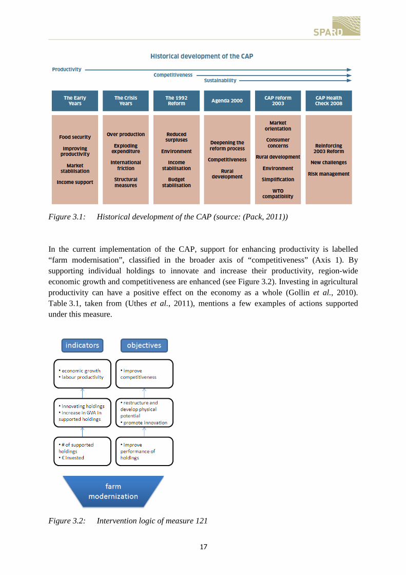
Productivity is a key factor on the Lisbon agenda, and so is cohesion (i.e., spatial equity). European support for investments in agricultural holdings started already in the mid-1960s, and it has always been a permanent instrument of the Common Agricultural Policy (CAP). Figure 3.1 (Uthes et al., 2011) shows further details on its history and juridical implementation.

17

Figure 3.1: Historical development of the CAP (source: (Pack, 2011))

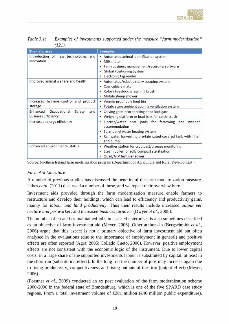
In the current implementation of the CAP, support for enhancing productivity is labelled “farm modernisation”, classified in the broader axis of “competitiveness” (Axis 1). By supporting individual holdings to innovate and increase their productivity, region-wide economic growth and competitiveness are enhanced (see Figure 3.2). Investing in agricultural productivity can have a positive effect on the economy as a whole (Gollin et al., 2010). Table 3.1, taken from (Uthes et al., 2011), mentions a few examples of actions supported under this measure.

Figure 3.2: Intervention logic of measure 121

18

Table 3.1: Examples of investments supported under the measure ”farm modernisation“ (121).

Thematic area Examples

Introduction of new technologies and

innovation

• Automated animal identification system

• Milk meter

• Farm business management/recording software

• Global Positioning System

• Electronic tag reader

Improved animal welfare and health

• Automated/robotic slurry scraping system

• Cow cubicle mats

• Rotary livestock scratching brush

• Mobile sheep shower

Increased hygiene control and product

storage

• Vermin proof bulk feed bin

• Potato store ambient cooling ventilation system

Enhanced Occupational Safety and

Business Efficiency

• Calving gate incorporating dead lock gate

• Weighing platform or load bars for cattle crush

Increased energy efficiency • Electric/water heat pads for farrowing and weaner

accommodation

• Solar panel water heating system

• Rainwater harvesting pre-fabricated covered tank with filter

and pump

Enhanced environmental status • Weather station for crop pest/disease monitoring

• Steam boiler for soil/ compost sterilization

• Quad/ATV fertiliser sower

Source: Northern Ireland farm modernization program (Department of Agriculture and Rural Development ).

Farm Aid Literature

A number of previous studies has discussed the benefits of the farm modernization measure. Uthes et al. (2011) discussed a number of these, and we repeat their overview here.

Investment aids provided through the farm modernization measure enable farmers to restructure and develop their holdings, which can lead to efficiency and productivity gains, mainly for labour and land productivity. Thus their results include increased output per hectare and per worker, and increased business turnover (Dwyer et al., 2008).

The number of created or maintained jobs in assisted enterprises is also sometimes described as an objective of farm investment aid (Meyer, 2006). Other authors in (Bergschmidt et al., 2006) argue that this aspect is not a primary objective of farm investment aid but often analysed in the evaluations (due to the importance of employment in general) and positive effects are often reported (Agra, 2005; Collado Cueto, 2006). However, positive employment effects are not consistent with the economic logic of the instrument. Due to lower capital costs, in a large share of the supported investments labour is substituted by capital, at least in the short run (substitution effect). In the long run the number of jobs may increase again due to rising productivity, competitiveness and rising outputs of the firm (output effect) (Meyer, 2006).

(Forstner et al., 2009) conducted an ex post evaluation of the farm modernization scheme 2000-2006 in the federal state of Brandenburg, which is one of the five SPARD case study regions. From a total investment volume of €201 million (€46 million public expenditure),

19

61% was spent for investments in agricultural buildings (29% for cattle sheds, 10% for pig pens, the remaining for other investments in buildings), 23% went to machinery and equipment, 14% to environmental investments (including photovoltaic systems, biogas plants) and the rest to other measures (e.g. young farmers aid 2%). Due to insufficient data (missing or incomplete accounting records, no time series), the authors conducted written and telephone interviews in combination with model-based analyses.

The interviews among the beneficiaries2 in Brandenburg (before-after comparison) indicated that labour productivity (87% of the surveyed farms), working conditions (85%), product quality (75%) as well as the farm income (75% positive or strongly positive, 13% however also slightly negative) were positively influenced by the investment aid. (Forstner et al., 2009) also found that the employment in supported farms had decreased by 13% (except for one farm that expanded production after the investment leading to 40 additional full employees). 65% of the surveyed farms had the opinion that the investment had somewhat lowered production costs, 67 % felt positive impacts on economic growth.

The authors found that the investments with environmental motivation (mostly machinery for improved slurry and pesticide application) were not very well targeted, a real impact assessment, however, was not possible due to lack of data. In addition, they reported positive impacts on animal welfare in the dairy sector (more space per animal) and negative impacts in the pig sector as the investments usually involved building fully concrete slatted floor pens.

A study in Belgium (Beck and Dogot), also based on questionnaires (n=17), found that the primary motivation for investment was improvement of working conditions (time saving for milking, feeding, better monitoring of animals, reduced stress and improved well-being for the animals) and to maintain the farming activity, and only to a lesser extent the improvement of farm income.

3.2 Theory and model

3.2.1 Guide for the analysis in SPARD

Uthes et al. (2011) discussed the appropriate method for the analysis of measure 121 in the current RDP programme (table 12). They noted in particular that this measure is one of the largest targets of RDP spending, covering over a tenth of the total budget across Europe, ranging from 3% in Ireland to 51% in Belgium. The total amount of money spent under this measure over the whole programming period (2007-2013) will be over €15 billion.

Following a literature survey and guided by expert insights, (Uthes et al., 2011) report that spill-over effects from RDP spending are not expected, and therefore our null hypothesis will be that there are none. One important reason why we would not expect large spill-over effects of this kind is that many NUTS2 areas coincide with planning regions for the RDP. However, we can think of two main ways in which spill-overs might occur of knowledge that influences productivity:

2 Interview sample size: 65 farms (= 4.1% of all beneficiaries); only farms with an investment volume of more

than 100.000 Euro were included; in total 1.586 cases were supported during the period 2000-2006

20

• by taking example: EU-funded modernization measures on one farm might be copied by neighbouring farms, or by farmers within a local network – where ‘local’ has no specific boundary, and certainly not the boundaries of an RDP; moreover, it is well known (even!) in spatial economics that proximity has other explanations than the obvious spatial one (Boschma, 2005; Torre and Rallet, 2005).

• by migration: some farmers might move their ‘business’ elsewhere, especially if they are not dependent on land or fixed assets. Many of the movers will move within a region, but some of them might cross a regional boundary. In some cases, a farmer who has scattered possessions might even receive money in one region but manage to spend part of it elsewhere.

Moreover, we will be able to test whether spatial heterogeneity exists - whether RDP spendings have different effects in different regions.

Hence, these effects can easily cross regional boundaries, especially where these do not coincide with physical or cultural separation (Newman and Paasi, 1998). Physical separation can hamper contact between otherwise similar regions; we can think of the IJsselmeer between North Holland and Friesland, or the Strait of Messina between Sicily and Calabria. Cultural separation is especially severe across country borders (Hussler, 2004), e.g. between Germany and Poland, and the more so with a language barrier; but language barriers even exist within countries, e.g. between the Flemish and the Walloon parts of Belgium.

There are, unfortunately, also reasons why the effect of RDP spending itself, without any spatial dimension, might appear less positive. Foremost is the displacement effect: if a subsidy to some farms makes these very competitive, they might actually push some of their competitors out of the market (especially if total demand stays constant, which is likely if the product itself does not change). Part of these competitors will be in the same region. A second risk is a deadweight effect: if subsidies replace investments that would have taken place anyway, the amount of subsidies will not change the outcome (Meyer, 2006).

One of the important aspects of almost any analysis is that of time. Three main problems arise. Firstly, the Mankiw-Romer-Weil model we will use as a base focuses on long-term structural developments in the economy, and thus we would like to use long periods. In doing so, we will also evade measuring business cycles, of which different types occur in agriculture, with some cycles lasting three, others a year and a half, some seven years, etc. (Coase and Fowler, 1935). (Da-Rocha and Restuccia, 2006) argue that agricultural activity fluctuates more and is not (positively) correlated with the rest of the economy. Secondly, the current RDP (“RDP2”) started only in 2007. Hence, the amount of years for which data is available is still small. We will therefore use data for the previous RDP period (2000-2006) as well, allowing us to analyse the period 2000-2010. Finally, investments in productivity increases take time. Previous research has shown that results are to be expected a minimum of 2-3 years after the investments (Forstner et al., 2009). Hence, we can only analyze results over longer time periods, and looking at short periods does not make sense. In this respect, we should also take into account that RDP spending only recently got underway in the newest members of the EU.

21

3.2.2 Model approach

Neoclassic growth models predict that, under certain conditions (complete markets, free entry and exit, negligible transaction costs, and convex technology relative to market size), countries and regions navigate a sea of economic opportunity that rewards productive efforts and savings (Solow, 1956). In the basic Solow model, economic growth is driven by savings and investments (in exogenous determined technologies). (Mankiw et al., 1992) add the human capital as an important factor. Other extensions are those of (Hall and Jones, 1999) that include the quality of the institutions, and Sachs and Warner (1997) adding (national trade policies). López-Bazo et al. (2004) address the effect of regional spillovers in the technology of production on the steady state level of capital and product and on the process of growth. The reasoning behind such spillovers is basically the diffusion of technology from other regions caused by investments in physical and human capital.

We base our model upon the basic (Solow, 1956)/(Swan, 1956) model as reproduced by (Mankiw et al., 1992) (henceforth MRW). This is a convenient model, but it is not the only way to model productivity. For example, (Hayami and Ruttan, 1970) (appendix; see discussion in (Huffman et al., 2001) p. 366) follow the approach where the wage in agriculture forms the basis of the approach, instead of capital, in a general CES production function. MRW define total production Y as a Cobb-Douglas function of capital (K), labour (L), and a modifying technological component (A). Basically, at time t:

"# � $#%(&#�#)'(%

�# � �)*+# &# � &)*�#

Effective labour A(t)L(t), which is L(t) modified by the amount of available technology A(t), grows at rate n+g; moreover, accumulation of capital enters as investments s (from ‘savings’). By assuming that each country is in or at a similar distance from its steady state, income per capita can then be derived to be

ln ."#�#

/ � ln &) � 01 2 �1 2 � ln(3 � 0 � �) � �

1 2 � ln(4) (1)

where &) represents an amount of technology, endowments, institutions, etc. available locally: in short, a parameter capturing all local influences on productivity. Mankiw, Romer & Weil take this factor to consist of a constant plus a random component, but other explanatory variables can be easily included (although this will make interpretation of the core variables less straightforward). On the other hand, depreciation δ and the exogenously assumed general growth of productivity g are supposed to be the same globally – in other words, technology is a pure public good.

Finally, n, is also a local parameter, denoting the growth rate of the local labour force. MRW explain that n (like s) has to be independent from the shock component of A (see below for remarks on interpreting n in a sectoral setting).

An extension MRW make to the Solow/Swan model is that they include human capital as a production factor. Using � as the parameter that gauges the importance of human capital H in total production, usually with � � � 6 1, they specify

22

"# � $#%7#8(&#�#)'(%(8 (2)

ln ."#�#

/ � ln &) � 01 2 � � �1 2 � 2 � ln(3 � 0 � �)

� �1 2 � 2 � ln(49) � �

1 2 � 2 � ln(4:)

(3)

in which 49 and 4: represent the fraction of income that is saved and automatically reinvested in capital and human capital, respectively. However, 4:, the increase in human capital, is not always available, and MRW propose to estimate the current level of human capital instead, assuming that level is at a steady state (p. 418):

ln ."#�#

/ � ln &) � 01 2 �1 2 � ln(3 � 0 � �)

� �1 2 � ln(49) � �

1 2 � ln(;∗)

(4)

Islam (1995, p. 1136) subsequently reformulated equation (1) to reflect a panel structure (eq. 11 in his article). Although the following equation appears to be still looking at levels, in fact it includes the lag of productivity on the right hand, and can easily be rewritten to explain the growth of productivity from year to year.3

ln =(1�) � >1 2 *?@A ln &) � 0(1� 2 *?@1')2 >1 2 *?@A �

1 2 � ln(3 � 0 � �)� >1 2 *?@A �

1 2 � ln(4) � *?@=(1')

(5)

where y is per capita income and � � (3 � 0 � �)(1 2 �). Translating a panel model to a spatial setting is not trivial, but huge progress has been made in this field over the last years, e.g. Anselin (2006), or the work by Elhorst (2003). However, since effects on productivity take time, as we discussed above, and we will have data for only eleven years, producing a spatial version of the Islam model falls outside the scope of this project. We will, however, split the sample into two periods, which may lead to hypotheses concerning the evolution of parameters over time.

3.3 Data, definitions and caveats

Data stem from a Cambridge Econometrics database, called the Regional Economic Model. This provides comprehensive data at the NUTS2 level, as well as a rather restricted dataset at the NUTS3 level. Cambridge Econometrics has employed “deflation, interpolation, and summation constraints” to make clean and verify the data, which is mainly based on the

3 Islands have no neighbours in a contiguity matrix, and thus form an econometric problem; see the section on

the weight matrix below.

23

Eurostat REGIO database. The data are available for 1980 to 2014, but data for the future are of course extrapolations from previous trends. We therefore restrict ourselves to the period 2000-2010.

For our analysis we will connect this database with two other data sources. First of all, we use data on RDP spending by NUTS2 region. This data was gathered by the European Commission in the so-called CATS database. This data is split by region and year, and to some degree also by objective or measure. Secondly, we will make use of Eurostat data, which has been conveniently bundled in the so-called MetaBase, developed by LEI (Dol and Godeschalk, 2011). From the enormous amount of available data there, we have selected some relevant proxies available at the NUTS2 level, including the size of agricultural holdings, the number of holdings with livestock, and the amounts of land (in % of total ha) used for pasture, woodland and vineyards, as well as the share of land in Less Favoured Areas.

Time and Space

The Cambridge Econometrics dataset and Eurostat both comprise 285 NUTS2 regions, covering the complete EU (including regions “d’outre-mer”), as well as Norway and Switzerland. For econometrics reasons, we restrict ourselves to regions within the European part of the EU, giving 263 regions.

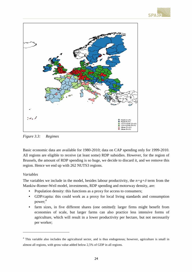
Because we expect both labour productivity and the effects of spending on rural development to vary across different types of regions, we distinguish six subregions within Europe, which we will call ‘regimes’ in the rest of this chapter (Figure 3.3). We define these six regions by population density (three classes, each with one third of the regions: urban, intermediate, and rural) and a north/south division. The latter can account for some climatic variation, but can also be linked to institutional quality.

24

Figure 3.3: Regimes

Basic economic data are available for 1980-2010; data on CAP spending only for 1999-2010. All regions are eligible to receive (at least some) RDP subsidies. However, for the region of Brussels, the amount of RDP spending is so huge, we decide to discard it, and we remove this region. Hence we end up with 262 NUTS3 regions.

Variables

The variables we include in the model, besides labour productivity, the n+g+δ term from the Mankiw-Romer-Weil model, investments, RDP spending and motorway density, are:

• Population density: this functions as a proxy for access to consumers; • GDP/capita: this could work as a proxy for local living standards and consumption

power;4 • farm sizes, in five different shares (one omitted): larger firms might benefit from

economies of scale, but larger farms can also practice less intensive forms of agriculture, which will result in a lower productivity per hectare, but not necessarily per worker;

4 This variable also includes the agricultural sector, and is thus endogenous; however, agriculture is small in

almost all regions, with gross value added below 2,5% of GDP in all regions.

25

• the share of family labour in total labour: the influence of family labour has been widely discussed in development economics, e.g. (Bardhan, 1973; Gershon, 1985), but its direction is not clear;

• the total share of agricultural land in the region: if this is low, farmers might have picked the best available soils, but they might also be spread further apart and have less benefits of networking or shared resources;

• the share of agricultural land in less favoured areas: if circumstances are bad, productivity is likely to be lower;

• and measures for some specific types of activities, namely woodlands, vineyards, flowers and livestock, which all have their specific technological and climatic differences..

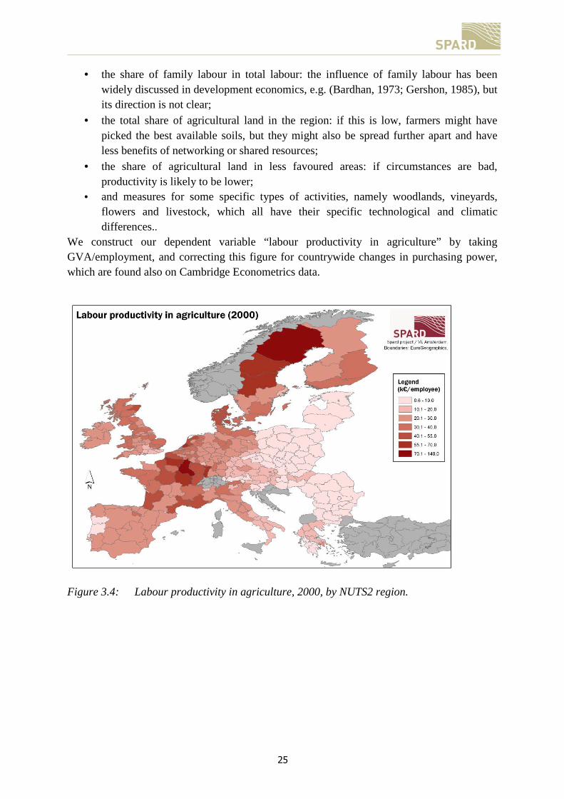
We construct our dependent variable “labour productivity in agriculture” by taking GVA/employment, and correcting this figure for countrywide changes in purchasing power, which are found also on Cambridge Econometrics data.

Figure 3.4: Labour productivity in agriculture, 2000, by NUTS2 region.

26

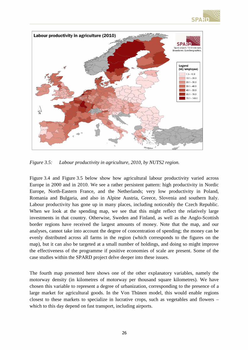
Figure 3.5: Labour productivity in agriculture, 2010, by NUTS2 region.

Figure 3.4 and Figure 3.5 below show how agricultural labour productivity varied across Europe in 2000 and in 2010. We see a rather persistent pattern: high productivity in Nordic Europe, North-Eastern France, and the Netherlands; very low productivity in Poland, Romania and Bulgaria, and also in Alpine Austria, Greece, Slovenia and southern Italy. Labour productivity has gone up in many places, including noticeably the Czech Republic. When we look at the spending map, we see that this might reflect the relatively large investments in that country. Otherwise, Sweden and Finland, as well as the Anglo-Scottish border regions have received the largest amounts of money. Note that the map, and our analyses, cannot take into account the degree of concentration of spending; the money can be evenly distributed across all farms in the region (which corresponds to the figures on the map), but it can also be targeted at a small number of holdings, and doing so might improve the effectiveness of the programme if positive economies of scale are present. Some of the case studies within the SPARD project delve deeper into these issues.

The fourth map presented here shows one of the other explanatory variables, namely the motorway density (in kilometres of motorway per thousand square kilometres). We have chosen this variable to represent a degree of urbanization, corresponding to the presence of a large market for agricultural goods. In the Von Thünen model, this would enable regions closest to these markets to specialize in lucrative crops, such as vegetables and flowers – which to this day depend on fast transport, including airports.

27

Figure 3.6: Annual average spending per holding, 2000-2010, by NUTS2 region.

Figure 3.7: Motorway density in km of motorway per 1000 km², by NUTS2 region.

28

Caveats

The RDP spending data we use is organized by year, but these years are not regular calendar years; instead, they start with three months in the previous calendar year, and then contain the first nine months of the given year. In other words, spending for 2010 refers to the period from October 2009 until September 2010. However, in some years the figures have been corrected for what apparently were mistakes or perhaps ex-post changes to previously allocated funding. In a handful of cases, this results in negative RDP spending for a particular year; in the analyses presented here, this does not pose an immediate problem, since we consider the total RDP spending over all 11 years, but it will lead to some imprecision, as the data are apparently organized by accounting year, which does not align perfectly with the moment of actual spending.

As for the regions used, the use of a Gabriel matrix allows us to keep all islands in the data; traditionally, they create problems particular to spatial econometrics (Anselin, 2002). Removing them is normally a straightforward solution, but it has the disadvantage of losing some information. However, we did choose to concentrate on the European part of the EU, removing information on the Spanish exclaves of Ceuta and Melilla (in Africa) as well as on the Portuguese Azores, but retaining the Canaries. We also dropped the city region of Brussels, as improbably high amounts of RDP spending are reported there, which we suspect to be due to accounting.

3.4 Results

In principle, Mankiw-Romer-Weil models focus on growth towards a steady-state, i.e. an equilibrium; hence its importance in literature on convergence (Abreu et al. 2005). However, we can also assume the status in a given year to be the steady state – i.e., there is a complete equilibrium – or that all regions are at the same distance from their respective steady states. This is a somewhat heroic assumption (surely there are still technological improvements, which for sound economic reasons will be implemented in rural Bulgaria in the near future), but it gives us an interesting background with which to compare our results of a growth analysis, which we will present below. When aiming to explain the productivity in the steady state, we would expect aspects such as the quality of the soil, hours of sunshine, level of technology and human capital to all affect the kind and efficiency of activities, and thus the labour productivity. However, when we move towards a growth model, the picture is fundamentally different, since we explain the dynamics. It is there that spatial effects, e.g. knowledge spillovers, can play an important role, but we will also test for them in the steady-state model.

Steady-state model

Our basic Mankiw-Romer-Weil model and the data we gathered is not aimed at explaining a steady-state; therefore, we do not expect the model to perform very well. Moreover, we cannot include RDP spending, since that assumes dynamics.5 The fact that it does render a

5 In theory, we can imagine a steady-state model that includes the total sum of all subsidies ever received.

29

high R squared (Table 3.2) is especially due to the country fixed effects. The OLS model (left-hand side) has some spatial dependence, indicated by the LM tests (bottom), but is indecisive whether this should be a spatial error or a spatial lag model – for reasons of interpretation and comparability, we estimate the latter, and these results are presented in the second column: here, where labour productivity in one region is influenced by a series of factors plus labour productivity in surrounding regions. Since this productivity of surrounding regions is in turn influenced by the same explanatory factors, indirect impacts are reported in the fifth column, and the total impact of the spatial model (i.e., coefficient + indirect effect) in the last column. Since the sign for � is positive, the indirect effects reinforce to some (small) degree the direct effects. Further details on the weight matrix, as well as a brief ESDA can be found below on page 32. The spatial model shows results similar to the regular OLS model. However, we should note that the estimates in the OLS model are not to be trusted as they stand; the LM tests prove there is spatial dependence, and thus OLS estimates are both inconsistent and biased.

Regarding individual variables, we see that the population density has a negative and significant effect on the labour productivity in agriculture. In other words, productivity seems to be lower in (urban) areas, with high population densities. Of course, this does not deny that labour-intensive activities are located near urban areas, but it does indicate that their labour productivity is lower. This is somewhat mitigated for regions that are easy to access by car/truck (motorway density), but still, our finding contradicts the theory of Von Thünen that intensive, profitable types of agriculture can take place just outside cities. Possibly, (environmental) restrictions and insufficient space to grow may cause this negative effect. Another explanation is that Von Thünens model does not apply to the spatial scale we have chosen; in the Netherlands, for example, where the NUTS2 level is defined by the twelve provinces, intensive horticulture might take place just outside Amsterdam and Rotterdam, but there are other types of agriculture in their provinces of North and South Holland as well, and the overall provincial productivity in both is less than in other Dutch provinces.

Regions with a higher income (GDP/capita) have a higher agricultural productivity per employee. When looking at the farm-related variables, we find the share of large farms in terms of acreage has a significant positive effect on the productivity, but the share of smallest farms also has this same effect, albeit only half as strong (the reference category is formed by farms of intermediate size, 10-30 ha). It is possible that this effect is caused by farms with a small area that actually grow intensive, high-yield crops; however, we should also remember we included country fixed effects, so that a general offset for some of the Eastern European countries is already provided in the model.

30

Table 3.2: Steady-state models. a-spatial model (OLS) spatial lag model

impact

Labour productivity in agriculture in 2010

(log) coefficient p-value coefficient

p-

value indirect total

GDP/capita 0.300 0.01 0.271 0.01 0.034 0.306

population density -0.183 0.00 -0.172 0.00 -0.021 -0.194

motorway density 0.005 0.00 0.005 0.00 0.001 0.005

% of tiny farms (<5 ha) 0.478 0.01 0.458 0.00 0.057 0.516

% of small farms (5-10 ha) 0.910 0.17 0.939 0.12 0.117 1.059

% of medium farms (30-50 ha) 0.549 0.42 0.534 0.39 0.066 0.602

% of large farms (>50 ha) 0.994 0.00 0.907 0.00 0.113 1.023

% of labour that is provided by family 0.002 0.99 -0.024 0.89 -0.003 -0.027

% of land that is utilized agricultural land 0.000 0.69 0.000 0.75 0.000 0.000

% of agricultural land in less favoured areas -0.002 0.00 -0.002 0.00 0.000 -0.003

% of surface that is woodlands -0.004 0.30 -0.003 0.32 0.000 -0.004

% of surface that is vineyards -0.029 0.21 -0.029 0.16 -0.004 -0.032

% of surface that is pastures 0.001 0.42 0.001 0.48 0.000 0.001

% of surface that is flowers 0.101 0.33 0.089 0.34 0.011 0.100

% of farms with livestock -0.418 0.03 -0.383 0.03 -0.048 -0.431

climate: mean minimum temp. in January 0.002 0.05 0.002 0.05 0.000 0.002

country fixed effects yes yes

observations 262 262

R² (adjusted) 0.82 0.83

Breusch-Pagan test 102 0.00 103 0.00

Rho 0.113 0.07

LM test Chi2-

value

p-

value

error model 5.71 0.02

lag model 3.60 0.06

robust error model 2.12 0.15

robust lag model 0.02 0.90

SARMA 5.73 0.06

When looking at environmental variables and the variables that indicate the use of land, we see that productivity is lower in less favoured areas – as was to be expected, and also for areas where there is more livestock, which may point to areas where soil or climate do not permit intensive agriculture. Note that if we would have had access to micro-data at farm level, we could compare farms in northern Scotland that attempt to grow vines with those that have sheep, and likewise on the Côte d’Azur, and we would probably find large differences. As the data stands, however, the choices what activities are deployed in a region are limited by soils and climate. Moreover, the inclusion of country fixed effects takes care of a lot of variation in climate and soil. However, we did construct one climate variable: from the daily minimum temperatures recorded (or reconstructed) per km² across Europe, we took the monthly average for January, and then the regional average by NUTS2 region. This variable had a slight but

31

statistically significant positive effect; in areas with warmer winters, productivity tends to be slightly higher. The effect is very small, and we refrained from constructing other variables. In an analysis on the production of specific crops with their own specific sensitivities (e.g., a minimum amount of sun in the growing season, no rain during the harvest, no frost in winter), more climate variables could and should be constructed.

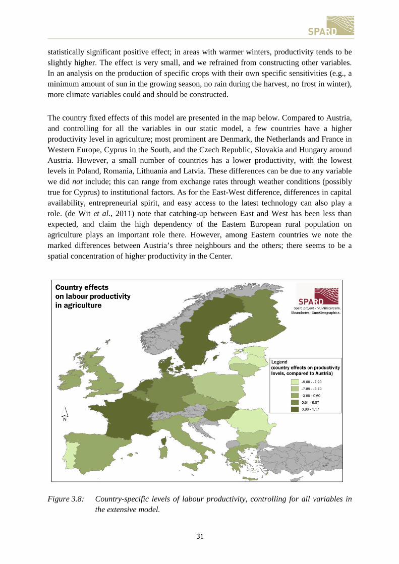
The country fixed effects of this model are presented in the map below. Compared to Austria, and controlling for all the variables in our static model, a few countries have a higher productivity level in agriculture; most prominent are Denmark, the Netherlands and France in Western Europe, Cyprus in the South, and the Czech Republic, Slovakia and Hungary around Austria. However, a small number of countries has a lower productivity, with the lowest levels in Poland, Romania, Lithuania and Latvia. These differences can be due to any variable we did not include; this can range from exchange rates through weather conditions (possibly true for Cyprus) to institutional factors. As for the East-West difference, differences in capital availability, entrepreneurial spirit, and easy access to the latest technology can also play a role. (de Wit et al., 2011) note that catching-up between East and West has been less than expected, and claim the high dependency of the Eastern European rural population on agriculture plays an important role there. However, among Eastern countries we note the marked differences between Austria’s three neighbours and the others; there seems to be a spatial concentration of higher productivity in the Center.

Figure 3.8: Country-specific levels of labour productivity, controlling for all variables in

the extensive model.

32

Growth models We estimate the growth model as productivity in 2010 related to productivity in 2000 and a series of variables influencing change, as in the standard MRW model. We also rewrite the model to explain the change in productivity from 2000 to 2010, but this makes no fundamental differences for the interpretation of the other explanatory variables; it does, however, allow a reinterpretation of the R² of the regression which is more realistic.6

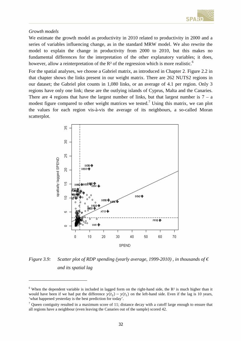
For the spatial analyses, we choose a Gabriel matrix, as introduced in Chapter 2. Figure 2.2 in that chapter shows the links present in our weight matrix. There are 262 NUTS2 regions in our dataset; the Gabriel plot counts in 1,080 links, or an average of 4.1 per region. Only 3 regions have only one link; these are the outlying islands of Cyprus, Malta and the Canaries. There are 4 regions that have the largest number of links, but that largest number is 7 – a modest figure compared to other weight matrices we tested.7 Using this matrix, we can plot the values for each region vis-à-vis the average of its neighbours, a so-called Moran scatterplot.

Figure 3.9: Scatter plot of RDP spending (yearly average, 1999-2010) , in thousands of €

and its spatial lag

6 When the dependent variable is included in lagged form on the right-hand side, the R² is much higher than it would have been if we had put the difference =(1�) 2 =(1') on the left-hand side. Even if the lag is 10 years, ‘what happened yesterday is the best prediction for today’. 7 Queen contiguity resulted in a maximum score of 11; distance decay with a cutoff large enough to ensure that all regions have a neighbour (even leaving the Canaries out of the sample) scored 42.

33

Figure 3.10: Scatter plot of labour productivity in agriculture (2010) and its spatial lag

Figure 3.9 and Figure 3.10 do this for RDP spending and labour productivity in agriculture, respectively. According to the figure Figure 3.9, there is a large number of regions with little spending, and their neighbours receive small sums as well. There are a few regions where a large amount of money is spent within the RDP (and from the maps reported above, we know these are for example some German regions), and most of these have neighbours that have also received above-average amounts of money. Observations with a large influence on the regression line are marked and labelled. Figure 3.9shows that there is a large cluster of observations around the average labour productivity, and sizeable groups of lower values Only a few observations are actually above this central cluster, most notably some Swedish regions. At the lower end of the scale, we see some Polish and British regions – since we correct for purchasing power, regions can have a similar labour productivity in our analysis, even if the real values differ widely.

The diagnostic LM tests (Anselin et al., 1996) are performed on the a-spatial model to test if the error terms show a spatial structure, see (Linderhof et al., 2011) for more details. They indicate there is scope for spatial econometrics in the first model, but as we proceed by differentiating both the base level (i.e., the constant) and the impact of spending by regimes, there is none left.

34

3.4.1 Results

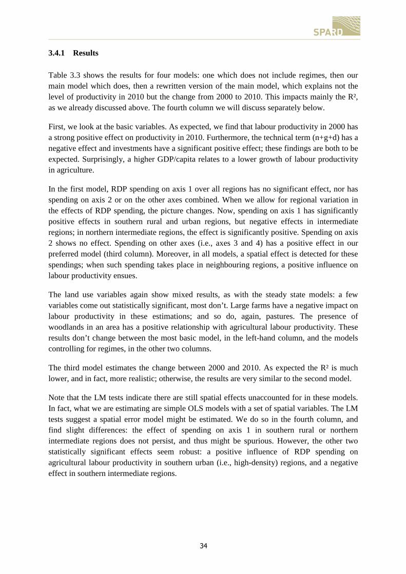
Table 3.3 shows the results for four models: one which does not include regimes, then our main model which does, then a rewritten version of the main model, which explains not the level of productivity in 2010 but the change from 2000 to 2010. This impacts mainly the R², as we already discussed above. The fourth column we will discuss separately below.

First, we look at the basic variables. As expected, we find that labour productivity in 2000 has a strong positive effect on productivity in 2010. Furthermore, the technical term (n+g+d) has a negative effect and investments have a significant positive effect; these findings are both to be expected. Surprisingly, a higher GDP/capita relates to a lower growth of labour productivity in agriculture.

In the first model, RDP spending on axis 1 over all regions has no significant effect, nor has spending on axis 2 or on the other axes combined. When we allow for regional variation in the effects of RDP spending, the picture changes. Now, spending on axis 1 has significantly positive effects in southern rural and urban regions, but negative effects in intermediate regions; in northern intermediate regions, the effect is significantly positive. Spending on axis 2 shows no effect. Spending on other axes (i.e., axes 3 and 4) has a positive effect in our preferred model (third column). Moreover, in all models, a spatial effect is detected for these spendings; when such spending takes place in neighbouring regions, a positive influence on labour productivity ensues.

The land use variables again show mixed results, as with the steady state models: a few variables come out statistically significant, most don’t. Large farms have a negative impact on labour productivity in these estimations; and so do, again, pastures. The presence of woodlands in an area has a positive relationship with agricultural labour productivity. These results don’t change between the most basic model, in the left-hand column, and the models controlling for regimes, in the other two columns.

The third model estimates the change between 2000 and 2010. As expected the R² is much lower, and in fact, more realistic; otherwise, the results are very similar to the second model.

Note that the LM tests indicate there are still spatial effects unaccounted for in these models. In fact, what we are estimating are simple OLS models with a set of spatial variables. The LM tests suggest a spatial error model might be estimated. We do so in the fourth column, and find slight differences: the effect of spending on axis 1 in southern rural or northern intermediate regions does not persist, and thus might be spurious. However, the other two statistically significant effects seem robust: a positive influence of RDP spending on agricultural labour productivity in southern urban (i.e., high-density) regions, and a negative effect in southern intermediate regions.

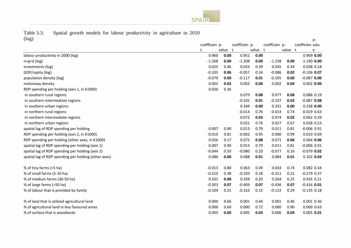
Table 3.3: Spatial growth models for labour productivity in agriculture in 2010 (log)

coefficien

t

p-

value

coefficien

t

p-

value

coefficien

t

p-

value

coefficien

t

p-

valu

e

labour productivity in 2000 (log) 0.960 0.00 0.951 0.00 0.969 0.00

n+g+d (log) -1.268 0.00 -1.208 0.00 -1.238 0.00 -1.190 0.00

investments (log) 0.025 0.46 0.033 0.39 0.035 0.34 0.038 0.18

GDP/capita (log) -0.105 0.06 -0.057 0.34 -0.086 0.02 -0.106 0.07

population density (log) -0.079 0.00 -0.117 0.01 -0.105 0.00 -0.087 0.00

motorway density 0.002 0.02 0.002 0.06 0.002 0.04 0.002 0.00

RDP spending per holding (axis 1, in €1000) 0.026 0.36

in southern rural regions 0.079 0.08 0.077 0.08 0.086 0.19

in southern intermediate regions -0.102 0.01 -0.107 0.02 -0.087 0.08

in southern urban regions 0.349 0.00 0.331 0.00 0.338 0.00

in northern rural regions -0.014 0.76 -0.014 0.74 -0.019 0.63

in northern intermediate regions 0.072 0.03 0.074 0.02 0.062 0.29

in northern urban regions 0.021 0.76 0.027 0.67 0.028 0.53

spatial lag of RDP spending per holding 0.007 0.90 0.013 0.79 0.011 0.81 -0.006 0.91

RDP spending per holding (axis 2, in €1000) -0.010 0.81 -0.002 0.95 0.000 0.99 0.010 0.69

RDP spending per holding (other axes, in €1000) 0.056 0.17 0.072 0.08 0.071 0.06 0.064 0.06

spatial lag of RDP spending per holding (axis 1) 0.007 0.90 0.013 0.79 0.011 0.81 -0.006 0.91

spatial lag of RDP spending per holding (axis 2) -0.044 0.50 -0.080 0.20 -0.077 0.16 -0.079 0.02

spatial lag of RDP spending per holding (other axes) 0.086 0.00 0.088 0.01 0.084 0.01 0.102 0.04

% of tiny farms (<5 ha) -0.013 0.80 0.063 0.49 0.034 0.74 0.082 0.34

% of small farms (5-10 ha) -0.210 0.38 -0.320 0.18 -0.311 0.21 -0.279 0.37

% of medium farms (30-50 ha) 0.501 0.08 0.359 0.20 0.264 0.25 0.435 0.21

% of large farms (>50 ha) -0.303 0.07 -0.409 0.07 -0.436 0.07 -0.416 0.01

% of labour that is provided by family -0.104 0.31 -0.163 0.15 -0.122 0.29 -0.135 0.18

% of land that is utilized agricultural land 0.000 0.66 0.001 0.44 0.001 0.46 0.001 0.36

% of agricultural land in less favoured areas 0.000 0.60 0.000 0.72 0.000 0.90 0.000 0.63

% of surface that is woodlands 0.005 0.00 0.005 0.03 0.006 0.04 0.005 0.01

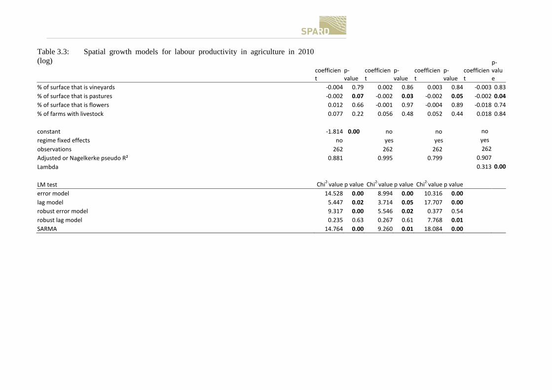
Table 3.3: Spatial growth models for labour productivity in agriculture in 2010 (log)

coefficien

t

p-

value

coefficien

t

p-

value

coefficien

t

p-

value

coefficien

t

p-

valu

e

% of surface that is vineyards -0.004 0.79 0.002 0.86 0.003 0.84 -0.003 0.83

% of surface that is pastures -0.002 0.07 -0.002 0.03 -0.002 0.05 -0.002 0.04

% of surface that is flowers 0.012 0.66 -0.001 0.97 -0.004 0.89 -0.018 0.74

% of farms with livestock 0.077 0.22 0.056 0.48 0.052 0.44 0.018 0.84

constant -1.814 0.00 no no no

regime fixed effects no yes yes yes

observations 262 262 262 262

Adjusted or Nagelkerke pseudo R² 0.881 0.995 0.799 0.907

Lambda 0.313 0.00

LM test Chi2-

value p value Chi2-

value p value Chi2-

value p value

error model 14.528 0.00 8.994 0.00 10.316 0.00

lag model 5.447 0.02 3.714 0.05 17.707 0.00

robust error model 9.317 0.00 5.546 0.02 0.377 0.54

robust lag model 0.235 0.63 0.267 0.61 7.768 0.01

SARMA 14.764 0.00 9.260 0.01 18.084 0.00

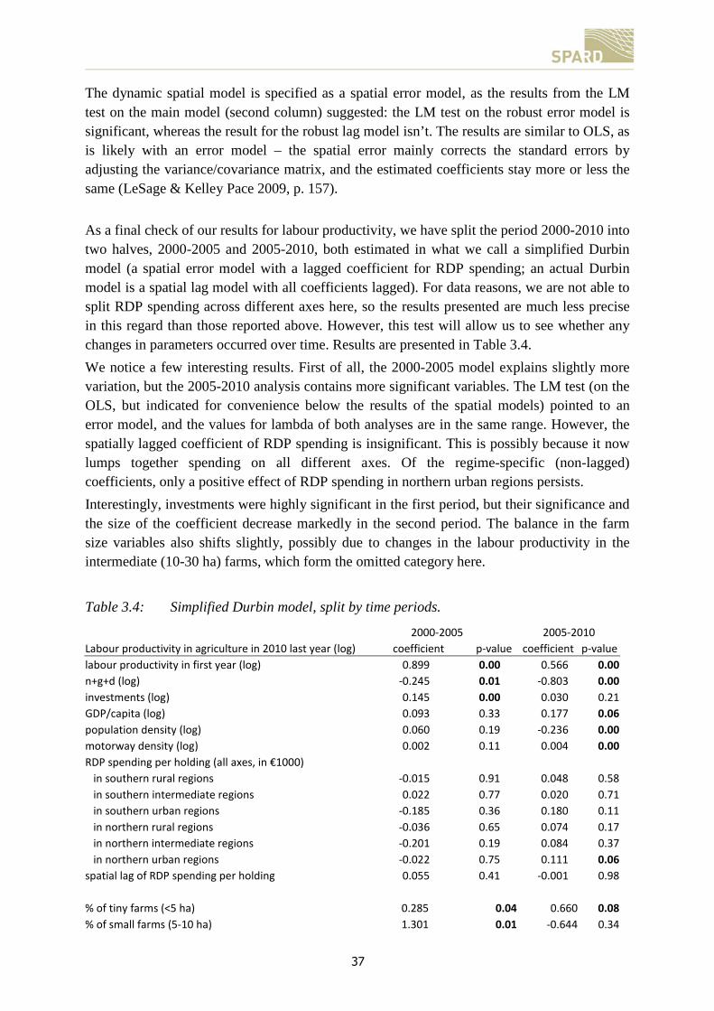
37

The dynamic spatial model is specified as a spatial error model, as the results from the LM test on the main model (second column) suggested: the LM test on the robust error model is significant, whereas the result for the robust lag model isn’t. The results are similar to OLS, as is likely with an error model – the spatial error mainly corrects the standard errors by adjusting the variance/covariance matrix, and the estimated coefficients stay more or less the same (LeSage & Kelley Pace 2009, p. 157).

As a final check of our results for labour productivity, we have split the period 2000-2010 into two halves, 2000-2005 and 2005-2010, both estimated in what we call a simplified Durbin model (a spatial error model with a lagged coefficient for RDP spending; an actual Durbin model is a spatial lag model with all coefficients lagged). For data reasons, we are not able to split RDP spending across different axes here, so the results presented are much less precise in this regard than those reported above. However, this test will allow us to see whether any changes in parameters occurred over time. Results are presented in Table 3.4.

We notice a few interesting results. First of all, the 2000-2005 model explains slightly more variation, but the 2005-2010 analysis contains more significant variables. The LM test (on the OLS, but indicated for convenience below the results of the spatial models) pointed to an error model, and the values for lambda of both analyses are in the same range. However, the spatially lagged coefficient of RDP spending is insignificant. This is possibly because it now lumps together spending on all different axes. Of the regime-specific (non-lagged) coefficients, only a positive effect of RDP spending in northern urban regions persists.

Interestingly, investments were highly significant in the first period, but their significance and the size of the coefficient decrease markedly in the second period. The balance in the farm size variables also shifts slightly, possibly due to changes in the labour productivity in the intermediate (10-30 ha) farms, which form the omitted category here.

Table 3.4: Simplified Durbin model, split by time periods.

2000-2005 2005-2010

Labour productivity in agriculture in 2010 last year (log) coefficient p-value coefficient p-value

labour productivity in first year (log) 0.899 0.00 0.566 0.00

n+g+d (log) -0.245 0.01 -0.803 0.00

investments (log) 0.145 0.00 0.030 0.21

GDP/capita (log) 0.093 0.33 0.177 0.06

population density (log) 0.060 0.19 -0.236 0.00

motorway density (log) 0.002 0.11 0.004 0.00

RDP spending per holding (all axes, in €1000)

in southern rural regions -0.015 0.91 0.048 0.58

in southern intermediate regions 0.022 0.77 0.020 0.71

in southern urban regions -0.185 0.36 0.180 0.11

in northern rural regions -0.036 0.65 0.074 0.17

in northern intermediate regions -0.201 0.19 0.084 0.37

in northern urban regions -0.022 0.75 0.111 0.06

spatial lag of RDP spending per holding 0.055 0.41 -0.001 0.98

% of tiny farms (<5 ha) 0.285 0.04 0.660 0.08

% of small farms (5-10 ha) 1.301 0.01 -0.644 0.34

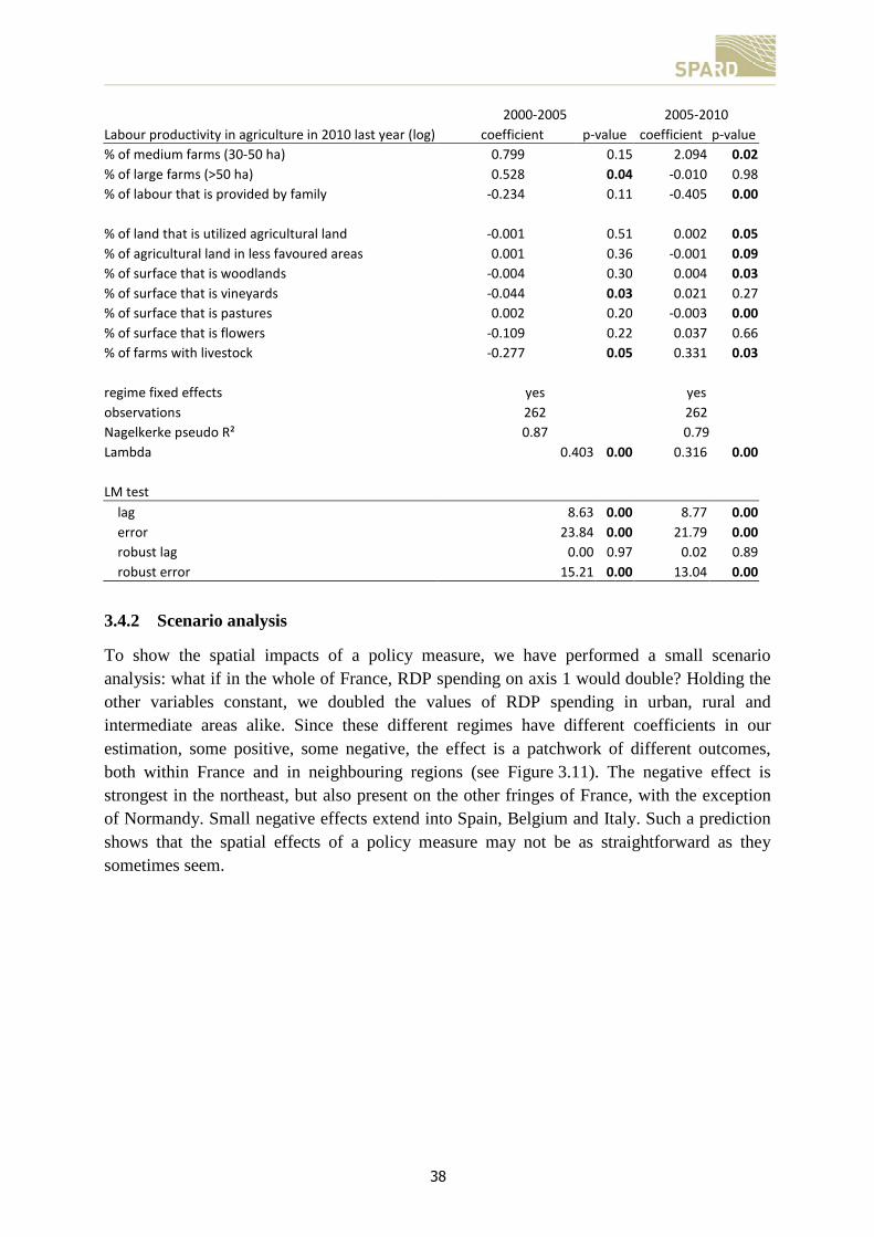
38

2000-2005 2005-2010

Labour productivity in agriculture in 2010 last year (log) coefficient p-value coefficient p-value

% of medium farms (30-50 ha) 0.799 0.15 2.094 0.02

% of large farms (>50 ha) 0.528 0.04 -0.010 0.98

% of labour that is provided by family -0.234 0.11 -0.405 0.00

% of land that is utilized agricultural land -0.001 0.51 0.002 0.05

% of agricultural land in less favoured areas 0.001 0.36 -0.001 0.09

% of surface that is woodlands -0.004 0.30 0.004 0.03

% of surface that is vineyards -0.044 0.03 0.021 0.27

% of surface that is pastures 0.002 0.20 -0.003 0.00

% of surface that is flowers -0.109 0.22 0.037 0.66

% of farms with livestock -0.277 0.05 0.331 0.03

regime fixed effects yes yes

observations 262 262

Nagelkerke pseudo R² 0.87 0.79

Lambda 0.403 0.00 0.316 0.00

LM test

lag 8.63 0.00 8.77 0.00

error 23.84 0.00 21.79 0.00

robust lag 0.00 0.97 0.02 0.89

robust error 15.21 0.00 13.04 0.00

3.4.2 Scenario analysis

To show the spatial impacts of a policy measure, we have performed a small scenario analysis: what if in the whole of France, RDP spending on axis 1 would double? Holding the other variables constant, we doubled the values of RDP spending in urban, rural and intermediate areas alike. Since these different regimes have different coefficients in our estimation, some positive, some negative, the effect is a patchwork of different outcomes, both within France and in neighbouring regions (see Figure 3.11). The negative effect is strongest in the northeast, but also present on the other fringes of France, with the exception of Normandy. Small negative effects extend into Spain, Belgium and Italy. Such a prediction shows that the spatial effects of a policy measure may not be as straightforward as they sometimes seem.

39

Figure 3.11: Scenario analysis

3.5 Discussion and conclusions

Proving the effects of spending from Rural Development Programme on regional labour and land productivity is not an easy thing. First of all, (micro)economic models – as most models – are simplifications of reality. Therefore it is difficult to adopt it to such a complex reality as regional labour productivity in agriculture. However, we do think that the MRW model we used is one of the best instruments for our purpose.

Other complications are the data on RDP spending. Since spending for 2010 refers to the period from October 2009 until September 2010 and, in some years the figures have been corrected for what apparently were mistakes or perhaps ex-post changes to previously allocated funding, this sometimes resulted in negative RDP spending for a particular year. In the analyses presented here, this does not pose an immediate problem, since we consider the total RDP spending over all 11 years or two periods, this does indicate likely imprecision in the data.

A final complication is the use of spatial weight matrices. The use of a Gabriel matrix allows us to keep all islands in the data; traditionally, they create problems particular to spatial econometrics (Anselin, 2002)). However, we dropped the city region of Brussels, as improbably high amounts of RDP spending are reported there, which we suspect to be due to accounting.

40

As for the role of spatial econometrics, we have shown using ESDA that agricultural labour productivity has a clear spatial pattern, and using LM tests that analyses that include spatial econometrics will be more accurate than regular estimations. However, when using the regimes, grouping similar regions, already a large share of the spatial relations were accounted for. From a policy perspective this implies that not taking spatial correlations into account may well be an acceptable second best strategy.

Important conclusions that we can draw from the analyses is that spending in general seems to have a positive effect on labour productivity; most strongly in southern rural and urban regions, and also in northern intermediate regions. The effect in southern intermediate regions seems to be negative. Another important conclusion is that spendings in axis 2 seems to have a negative effect on labour productivity. This counter effect should be taken serious by policy makers.

Finally, the effect of spendings on axis 1 and 2 in neighbouring regions seems to be very small or non-existent, at least for labour productivity, in a timeframe of 10 years, at the NUTS2 level. However, spill-over effects of spending on the other axes appear to be positively significant. Further research might be needed to indicate if this is desirable or not from the perspective of the objectives of the other axes.

The additional models in which the time period is split up in 2000-2005 and 2005-2010 give us an important warning. The spending variables show different results: most of the significant effects disappear. This can be explained by the fact that this model only handles total spending, not correcting for axis 1 and 2, and thus it underlines the importance of taking into account the separate axes.

41

4 Environmental model

4.1 Introduction

This chapter deals with measure 214 (improving the environment and the countryside) and consists of agri-environmental measures (AEM). It is the most important measure within RDP. Of the total public budget, almost a quarter (23.6%) is allocated to this measure (35 billion including EU and national contribution). The measure is offered in all 27 EU Member States. The relative share in total public RD budget ranges from 46.3% (Ireland) to less than 6.8% in Latvia. Highest farmer uptake is found in extensive agricultural regions (mountainous areas, grassland areas), whereas low implementation occurs in prime agricultural regions. Measure 214 consists of an array of different measures for which the degree of implementation varies largely among the Member States and regions.

Figure 4.1: Spending per hectare per NUTS2 region on measure 214 in 2010

AEM are contracts between farmers and the governing authority, in which farmers commit themselves – usually for a five-year minimum period – to adopt environmentally friendly farming practices that go beyond usual good agricultural practice. In return, they receive payments that compensate for additional costs and loss of income that result from altered farming practices (Com, 2005). AEM are a mandatory component of the RDPs (Com, 2005). The majority of AEM aims at taking action rather than achieving environmental results (Uthes et al., 2011). Measure 214 can be seen as a stimulus for farmers to deviate from optimal agricultural practice to enlarge the positive effects for society. These societal benefits are improvements of water quality and biodiversity (the objectives of RDP).

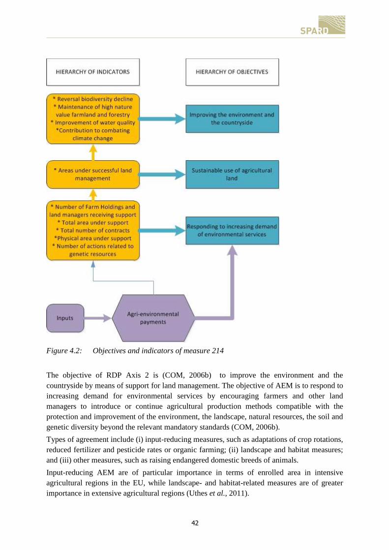
42

Figure 4.2: Objectives and indicators of measure 214

The objective of RDP Axis 2 is (COM, 2006b) to improve the environment and the countryside by means of support for land management. The objective of AEM is to respond to increasing demand for environmental services by encouraging farmers and other land managers to introduce or continue agricultural production methods compatible with the protection and improvement of the environment, the landscape, natural resources, the soil and genetic diversity beyond the relevant mandatory standards (COM, 2006b).

Types of agreement include (i) input-reducing measures, such as adaptations of crop rotations, reduced fertilizer and pesticide rates or organic farming; (ii) landscape and habitat measures; and (iii) other measures, such as raising endangered domestic breeds of animals.

Input-reducing AEM are of particular importance in terms of enrolled area in intensive agricultural regions in the EU, while landscape- and habitat-related measures are of greater importance in extensive agricultural regions (Uthes et al., 2011).

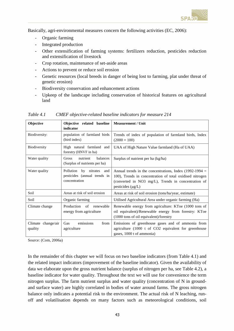
43

Basically, agri-environmental measures concern the following activities (EC, 2006):

- Organic farming

- Integrated production

- Other extensification of farming systems: fertilizers reduction, pesticides reduction and extensification of livestock

- Crop rotation, maintenance of set-aside areas

- Actions to prevent or reduce soil erosion

- Genetic resources (local breeds in danger of being lost to farming, plat under threat of genetic erosion)

- Biodiversity conservation and enhancement actions

- Upkeep of the landscape including conservation of historical features on agricultural land

Table 4.1 CMEF objective-related baseline indicators for measure 214

Objective Objective related baseline indicator

Measurement / Unit

Biodiversity:

population of farmland birds (bird index)

Trends of index of population of farmland birds, Index (2000 = 100)

Biodiversity High natural farmland and forestry (HNVF in ha)

UAA of High Nature Value farmland (Ha of UAA)

Water quality

Gross nutrient balances (Surplus of nutrients per ha)

Surplus of nutrient per ha (kg/ha)

Water quality

Pollution by nitrates and pesticides (annual trends in concentration

Annual trends in the concentrations, Index (1992-1994 = 100), Trends in concentration of total oxidised nitrogen (converted in NO3 mg/L), Trends in concentration of pesticides (µg/L)

Soil Areas at risk of soil erosion Areas at risk of soil erosion (tons/ha/year, estimate)

Soil Organic farming Utilised Agricultural Area under organic farming (Ha)

Climate change Production of renewable energy from agriculture

Renewable energy from agriculture: KToe (1000 tons of oil equivalent)/Renewable energy from forestry: KToe (1000 tons of oil equivalent)/forestry

Climate change/air quality

Gas emissions from agriculture

Emissions of greenhouse gases and of ammonia from agriculture (1000 t of CO2 equivalent for greenhouse gases, 1000 t of ammonia)

Source: (Com, 2006a)

In the remainder of this chapter we will focus on two baseline indicators (from Table 4.1) and the related impact indicators (improvement of the baseline indicator). Given the availability of data we elaborate upon the gross nutrient balance (surplus of nitrogen per ha, see Table 4.2), a baseline indicator for water quality. Throughout the text we will use for convenience the term nitrogen surplus. The farm nutrient surplus and water quality (concentration of N in ground- and surface water) are highly correlated in bodies of water around farms. The gross nitrogen balance only indicates a potential risk to the environment. The actual risk of N leaching, run-off and volatilisation depends on many factors such as meteorological conditions, soil

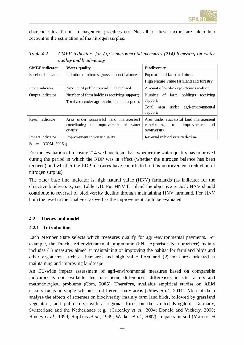
44

characteristics, farmer management practices etc. Not all of these factors are taken into account in the estimation of the nitrogen surplus.

Table 4.2 CMEF indicators for Agri-environmental measures (214) focussing on water quality and biodiversity

CMEF indicator Water quality Biodiversity

Baseline indicator Pollution of nitrates, gross nutrient balance Population of farmland birds,

High Nature Value farmland and forestry

Input indicator Amount of public expenditures realised Amount of public expenditures realised

Output indicator Number of farm holdings receiving support;

Total area under agri-environmental support;

Number of farm holdings receiving support;

Total area under agri-environmental support;

Result indicator Area under successful land management contributing to improvement of water quality.

Area under successful land management contributing to improvement of biodiversity

Impact indicator Improvement in water quality Reversal in biodiversity decline

Source: (COM, 2006b)

For the evaluation of measure 214 we have to analyse whether the water quality has improved during the period in which the RDP was in effect (whether the nitrogen balance has been reduced) and whether the RDP measures have contributed to this improvement (reduction of nitrogen surplus)

The other base line indicator is high natural value (HNV) farmlands (as indicator for the objective biodiversity, see Table 4.1). For HNV farmland the objective is dual: HNV should contribute to reversal of biodiversity decline through maintaining HNV farmland. For HNV both the level in the final year as well as the improvement could be evaluated.


4.2.1 Introduction

Each Member State selects which measures qualify for agri-environmental payments. For example, the Dutch agri-environmental programme (SNL Agrarisch Natuurbeheer) mainly includes (1) measures aimed at maintaining or improving the habitat for farmland birds and other organisms, such as hamsters and high value flora and (2) measures oriented at maintaining and improving landscape.

An EU-wide impact assessment of agri-environmental measures based on comparable indicators is not available due to scheme differences, differences in site factors and methodological problems (Com, 2005). Therefore, available empirical studies on AEM usually focus on single schemes in different study areas (Uthes et al., 2011). Most of them analyse the effects of schemes on biodiversity (mainly farm land birds, followed by grassland vegetation, and pollinators) with a regional focus on the United Kingdom, Germany, Switzerland and the Netherlands (e.g., (Critchley et al., 2004; Donald and Vickery, 2000; Hanley et al., 1999; Hopkins et al., 1999; Walker et al., 2007). Impacts on soil (Marriott et

45

al., 2005), (Deumlich et al., 2006), water (Granlund et al., 2005; Hodge, 2000; Parrott and Burningham, 2008), and air (Peerlings and Polman, 2008) are less often addressed (Uthes et al., 2011).

The experience with agri-environmental measures shows that they have patchy success (Anselin, 2006; Kleijn et al., 2006; Sutherland, 2004) depending on the schemes and indicators under investigation (Uthes et al., 2011). There is some evidence for AEM reversing negative trends in bird monitoring data (Brereton et al., 2008), particularly in diversified, small-scale landscapes (Bullock et al., 2007; Edwards et al., 2007; Hopkins et al., 1999)}. AEM have effectively targeted suitable habitats in the UK (Carey et al., 2005), but were less successful in targeting erosive sites in Germany (Deumlich et al., 2006). Grassland extensification in Switzerland has had positive effects on pollinator species richness and abundance and pollination services to nearby intensely managed farmland (Albrecht et al., 2007). A study in the Netherlands found no positive effects on plant and bird species diversity, while hover flies and bees showed modest increases (Kleijn et al., 2001). Studies in intensive regions usually reported less successful results and concluded that much more and different conservation efforts are needed (Herzog et al., 2005; Kleijn, 2006). Available studies of impacts on abiotic resources reported unsatisfactory results (Granlund et al., 2005).

If the causes of environmental problems are not well-known and schemes therefore might not be appropriately designed, AEM can also have unintended effects. Impacts on biodiversity, for example, are influenced by many factors, such as habitat quality, nutrient supply, groundwater levels, forage availability, disturbances (scaring), and landscape (Uthes et al., 2011). (Kleijn et al., 2001) report a scheme in the Netherlands in which grassland extensification with delayed cutting caused a lower availability of food (soil invertebrates) for bird species. Birds consequently preferred conventional fields as forage areas. It was concluded that the lower food availability caused the birds to perceive such sites as poor-quality nesting habitat (despite a potentially higher survival rate of juveniles). The management prescriptions of the scheme were obviously not appropriately designed for the conditions in that particular landscape and the needs of that bird species, leading to a decoupling effect between nesting habitat and reproductive effect. Another example was given in (Bro et al., 2004), who analysed the biodiversity effects of wildlife cover strips. These authors found that, under certain circumstances, cover strips concentrate the number of species within small isolated areas and may therefore act as an ecological trap for prey species such as the grey partridge. A weak scheme design can also cause trade-offs between different ecological objectives, e.g. between biodiversity and arboriculture (tree care) if the time of tree cuts overlaps with the breeding period of field birds (Bussler et al., 2006).

(Hodge and Reader, 2009) criticize the failure of schemes in the UK to include prescriptions for maintaining hedges and ditches and the lack of water level prescriptions included in wetland restoration program (Hodge and McNally, 1998). In a later publication, these authors therefore recommend more room for collective actions to effectively control the water level in such programs (Hodge and McNally, 2000). (Bailey, 2007) reports as a negative effect that increasing connectivity networks, especially those with corridors, may function as conduits for undesirable species or disease spread. This invasion of habitats by non-target species can compromise conservation goals (Baer et al., 2009). Invasion is promoted by legacies of

46

disturbance, landscape factors, novel plant communities and the absence of ecological drivers that historically maintained target communities (Baer et al., 2009) and also by climate change (Ausden and Fuller, 2009).

4.2.2 Spillover effects

Water quality

In SPARD we are interested in the spatial dependence of the impact of agri-environmental measures. The most prominent element of spatial dependence is spillover. Water quality has a distinctive spillover effect. For example pollution emitted to a river upstream will flow downstream and pollute the water on its way to the sea (until it is diluted sufficiently). Assuming that the NUTS regions are not defined based on the watersheds, water quality is a clear example of a spillover. The water quality in a region affects the adjacent regions downstream. If we want to model this spatial econometrically the weight matrix has to be defined according to the direction of the water flow. The spatial lag model is the appropriate model in which the parameter rho captures the dilution of pollution. (water and its quality is not tied to one region).

In our model we use nitrogen surplus as a baseline indicator. Nitrogen surplus is defined as the nitrogen surplus per hectare, it is therefore tied to a territorial unit. As presented in Figure 4.3 nitrogen surplus is affected by various processes and is computed based on several variables, of which a few have a spillover. Deposition of nitrogen (by air) is a clear spillover, it is caused by nitrogen emissions on other locations. Largest portion of nitrogen surplus is defined at the regional level by the production intensity of the farms. If we assume that the type of farming does not change a lot across the border there is some spatial relation (but no physical spillover). Transport of manure, from farms with a manure surplus towards farms with a manure deficit, is included in the data thus also a direct spillover exists.

Biodiversity

Biodiversity also has a spatial spillover. Animals are free to migrate across the border of regions (the actual rate of which animals will cross the border largely depends on the specie). Birds will more easily cross borders than reptiles. We used the HNV farmland indicator as an proxy for biodiversity. The variables that determine the HNV indicator are spatially determined by the region itself (see Section 4.3.2) and have no direct spillover effect, although the indicator that is simulated has. If we explain the HNV indicator we do not model spillovers.

4.2.3 Model

Water quality

Several AEM aim to reduce the use of nutrients (e.g. organic farming, extensification of grassland, application of better techniques), decreasing the emission of nutrients to the environment and improving water quality. Emissions to the environment can be described by

47

the nitrogen surplus as the indicator for measure 214. Nitrogen surplus is in the CMEF indicators coupled to water quality (table 4.2). AEM will substitute the environmentally detrimental output nitrogen surplus for inputs (for instance extra labour or more expensive machinery) and/or a reduction of the agricultural production.

Agricultural production can be modelled by a production function relating agricultural production to inputs (equation 4.1). This production function is an extended version of the standard production function alike the one presented in paragraph 3.2.2. In equation 4.1 the environment and the entrepreneur are added (Antle and Capalbo, 2001; Neumann et al., 2010; Reinhard et al., 1999)

.

" � B(�, $, D, E, F, G, H) (4.1)

Where:

Y = Agricultural production

L = (family) labour input (a quasi-fixed input)

K = Capital input (buildings, machinery), private investments (a quasi-fixed input)

G = land input (in ha; a quasi-fixed input)

V = Variable inputs (fertilizer, feed, etcetera)

S = Site specific characteristics (soil quality, slope, weather conditions, institutions)

M = Managerial quality

N = Emissions to the environment (e.g. nitrogen surplus).

To evaluate the relation between the baseline indicator nitrogen surplus and the expenditures on measure 214, a transformation of equation 4.1 is preferable to obtain a specification where the baseline indicator is the dependent variable. Emissions to the environment (N) are an undesirable output and can be modelled as an input (Reinhard, 1999). We assume a positive relationship between the environmentally detrimental output N and the market output Y, and a negative relationship between N and the other inputs (N surplus and the inputs are considered substitutes).

An input demand function for nitrogen surplus (that relates nitrogen surplus to expenditures on 214) is the perfect candidate for the equation to be estimated. The duality property between cost and production functions (based on Shephard’s Lemma) can be used to derive input demand equations (Diewert, 1971). The production function and cost have to fulfil regularity conditions implied by economic theory (Diewert, 1974). The usual strategy is to choose a flexible functional form for the cost function and then use Shephard’s Lemma to derive a set of factor share, input demand equations which is linear in the parameters. The corresponding input demand functions (multiple inputs and one output) relates the input to the output, the quasi-fixed inputs and the prices of all variable inputs (Kumbhakar, 1994; O'Donnell et al., 1999).

A market price for nitrogen surplus does not exist. We also do not have data available on prices of the variable inputs (see section 4.3.1). These missing data restrict the possibilities to specify the input demand equations. We choose, given the available data, for an input demand

48

function specification (O'Donnell et al., 1999), using output quantity, quasi-fixed inputs quantity (capital and labour) and a country specific effect (we use panel data) to capture country specific physical conditions and efficiency. As we have only quantity data on one variable input (nitrogen surplus per hectare), we estimate one ad hoc input demand function. We will test the basic underlying assumptions.

The dependent variable is the baseline indicator nitrogen surplus per hectare (kg N/ha), therefore we divide all variables in equation (4.1) by the relevant acreage. The land variable can be omitted in our analysis, see Section 4.4.1. We compare regions in the EU, hence we include a variable that incorporates site specific characteristics to model productivity differences throughout the EU. If regions are analysed the average managerial quality can be regarded as a regional specific variable and can be included in the variable, S.

H � B(", �, $, E, F) (4.2)

To test the hypotheses that RDP-measures affect the change of the baseline indicator, we have to estimate the aforementioned functions (4.2). A specification has to be selected (due to data limitations we shall not derive this input demand function formally from the corresponding cost function). A flexible function form is warranted to allow for diminishing rate of returns of inputs. The Cobb-Douglas and quadratic specifications are the most commonly used types of farm production, and have been shown to give similar results. Unlike the Cobb-Douglas method, the quadratic form allows for decreasing returns and can handle zero values for input or output variables, yet multicollinearity is a frequently encountered problem. The Cobb-Douglas function, on the other hand, tends to give better results if inputs and outputs have a high variation, as logarithmic transformation reduces the spread in values (Grovermann et al., 2012). The Cobb-Douglas production function form is chosen. A disadvantage of a Cobb-Douglas production function is that is specified in logarithms that do not allow for negative values (that are possible in year to year change in nitrogen surplus). We deal with this problem in section 4.30.

Agricultural Biodiversity

Farmers are subsidized via AEM to maintain or improve landscape elements or nature areas (e.g. erosion protection measures, hedgerow maintenance). These measures will decrease the productive capacity of agricultural land, and improve the quantity and quality of landscape elements (by providing an income for their time spent to landscape maintenance). Various AEM affect the joint agricultural production of produce and landscape amenities, see (Wiggering et al., 2006).

B(", &) � B(�, $, GF, D, E, F, G, H) (4.3)

Where:

A = Rural amenities (e.g. landscape and agricultural biodiversity)

49

We model rural amenities (A) as a joint output. Agricultural yield can be substituted for agricultural biodiversity. We do not have actual data on agricultural biodiversity and use a constructed index based on farm structural characteristics (see 4.3.2). We also have limited data on inputs. Therefore, we do not derive the agricultural biodiversity function (equation 4.4) formally, but apply a more pragmatic approach, but will test the basic underlying assumptions.

& � B(", �, $, GF, D, E, F, G, H) (4.4)

We assume a negative relationship between agricultural biodiversity and the market output Y, and a positive relationship between agricultural biodiversity (A) and the inputs. The effect that RDP measures have on the related RDP objectives is measured in SPARD using spatial econometrics. The change of the impact indicator (the dependent variable) is related to the RDP spending (one of the independent variables).


4.3.1 Impact on water quality

Water quality is not measured consistently throughout the EU and cannot be used as a suitable indicator. The impact indicator defined in the handbook on CMEF is changes in gross nutrient balance. The gross nutrient balance indicates potential nutrient losses to the water bodies likely to be detrimental for the quality of water. Important water quality problems in EU rural areas are the high concentrations of nutrients in ground- and surface waters. These nutrients stem from excess application of nitrogen en phosphorus to crops due to application of manure and fertilizer. The water quality is highly affected by agricultural nitrogen use. In the remainder of this Chapter, we focus on nitrogen surplus.

The gross nitrogen balance provides an insight into the links between agricultural nitrogen (N) use, losses of N to the environment, and the sustainable use of soil N resources8. Part of the applied nitrogen (in fertilizer and manure), is taken up by crops, but a large portion of these nutrients is emitted to the environment (nitrogen is emitted to the air and soil; and from the soil into the ground water).

8 See: http://epp.eurostat.ec.europa.eu/statistics_explained/index.php/Nitrogen_balance_in_agriculture

50

Figure 4.3: Scheme for the nitrogen cycle including gross nitrogen surplus

The gross nitrogen balance indicates the amount of nitrogen that can be potentially emitted into the water and should be interpreted as a potential risk indicator for water quality. A persistent N surplus indicates a potential risk of N leaching, run-off and volatilisation to water, soil and air. A persistent deficit indicates a potential risk of decline in soil fertility. The gross nitrogen surplus is computed as equation 4.5, based on farm accounts: yield and input use (Reinhard, 1999).

outputsNinputsNsurpN ___ −= (4.5)

Where

N_surp = Nitrogen surplus (in kgN/year)

N_inputs = Nitrogen in inputs (fertilizer, manure, feed) (in kgN/year)

N_outputs = Nitrogen in outputs (milk, wheat, potatoes, roughage) (in kgN/year)

There are too many variables influencing the transfer of nutrients from the soil to the water bodies to establish a direct and simple relationship between gross nitrogen balance and nitrogen concentration in the water at an aggregate level (see figure 4.3). The actual risk of N leaching, run-off and volatilisation depends on many factors such as meteorological conditions, soil characteristics, farmer management practices etc. These factors are not all taken into account in the estimation of the gross nitrogen balances. The gross nitrogen surplus shows the link between agricultural activities and the environmental impact, identifying the factors determining nitrogen surpluses or deficits and the trends over time.

Data

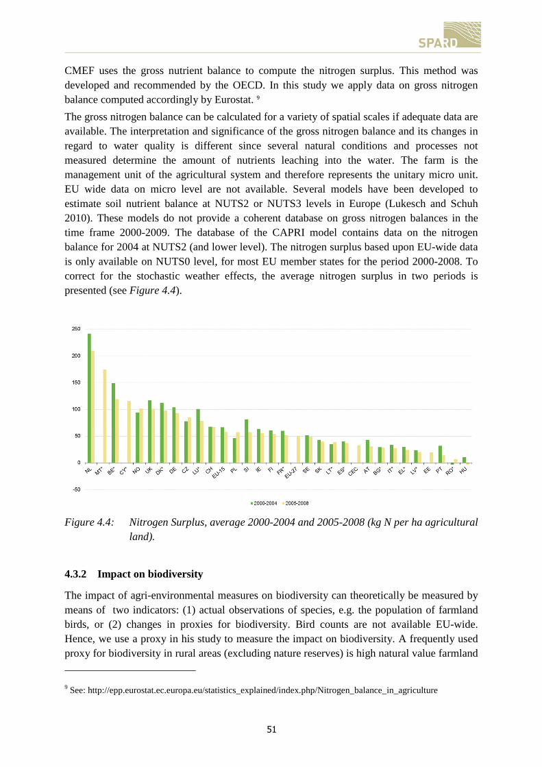
51

CMEF uses the gross nutrient balance to compute the nitrogen surplus. This method was developed and recommended by the OECD. In this study we apply data on gross nitrogen balance computed accordingly by Eurostat. 9

The gross nitrogen balance can be calculated for a variety of spatial scales if adequate data are available. The interpretation and significance of the gross nitrogen balance and its changes in regard to water quality is different since several natural conditions and processes not measured determine the amount of nutrients leaching into the water. The farm is the management unit of the agricultural system and therefore represents the unitary micro unit. EU wide data on micro level are not available. Several models have been developed to estimate soil nutrient balance at NUTS2 or NUTS3 levels in Europe (Lukesch and Schuh 2010). These models do not provide a coherent database on gross nitrogen balances in the time frame 2000-2009. The database of the CAPRI model contains data on the nitrogen balance for 2004 at NUTS2 (and lower level). The nitrogen surplus based upon EU-wide data is only available on NUTS0 level, for most EU member states for the period 2000-2008. To correct for the stochastic weather effects, the average nitrogen surplus in two periods is presented (see Figure 4.4).

Figure 4.4: Nitrogen Surplus, average 2000-2004 and 2005-2008 (kg N per ha agricultural

land).

4.3.2 Impact on biodiversity

The impact of agri-environmental measures on biodiversity can theoretically be measured by means of two indicators: (1) actual observations of species, e.g. the population of farmland birds, or (2) changes in proxies for biodiversity. Bird counts are not available EU-wide. Hence, we use a proxy in his study to measure the impact on biodiversity. A frequently used proxy for biodiversity in rural areas (excluding nature reserves) is high natural value farmland

9 See: http://epp.eurostat.ec.europa.eu/statistics_explained/index.php/Nitrogen_balance_in_agriculture

52

and forestry (HNV). Such land types comprise the hot spots of biological diversity in rural areas. They are often characterised by extensive farming practices, associated with a high species and habitat diversity or the presence of species of European conservation interest (Paracchini, 2006). In the definition given by (Andersen et al., 2003), HNV farmland is described as: ‘those areas in Europe where agriculture is a major (usually the dominant) land use and where that agriculture supports or is associated with either a high species and habitat diversity or the presence of species of European conservation concern or both’.

HNV farmland refers to farmland characterised by the presence if particular land cover types and patterns (especially semi-natural vegetation and low-intensity crop mosaics) which indicate that this farmland is valuable for nature conservation. The presence of populations of particular wildlife species may also provide this indication. HNV farmland may exist at different scales, from the individual parcel to the entire landscape. The HNV farmland guidance document (EC, 2009) emphasises that the idea of the indicator is not to design particular areas or zones as HNV farmland. The idea of the HNV concept is to contribute to nature conservation by supporting and maintaining the broad types of farming (and forestry) characteristics that are known to be critical for supporting nature values, and which then provide the basis for identifying HNV farmland on the ground (Lukesch and Schuh, 2010).

The overall challenge for Member States in order to implement this CMEF indictor is to - Devise a set of indicators that will provide meaningful information on changes in the

extent and in the condition of HNV farmland, and on trends in HNV systems and practices, during the seven years of the Rural Development Programme

- Devise a method for assessing to what extent (and how) these changes and trends have been influenced by RD programmes and measures.

Member States have not yet established a satisfactory method of indicators for HNV farmland. There are many challenges to overcome. Severe data limitations exist at present which make it very difficult to specify a computable HNV indicator at the level of entire countries or regions. The data required are not available to distinguish the full range of HNV farmland characteristic at the level of land parcel or farm holding, or to map their distribution with accuracy across an entire region. Several HNV farmland indicators have been developed and computed at member state of regional level; Lukesch and Schuh (2010) present an overview of examples. For instance Germany has taken the sampling approach to monitoring HNV farmland. About 1,000 sites of each 100 ha are included in the survey. An EU-wide indicator is not available. Therefore the impact of RDP spending on this HNV indicator has not been established yet. In order to be able to do so in SPARD, we defined a HNV-indicator (especially for this project) that could be computed for a majority of the NUTS2 regions. In order to be able to do so in SPARD, we defined a HNV-indicator (especially for this project) that could be computed for a majority of the NUTS2 regions. Our HNV indicator is not approved by the EU and should not be taken as indicator in official evaluations. It is only applied in this document to show the potential of spatial econometrics.

Among other factors, the type of agriculture is relevant for biodiversity (Paracchini and Britz, 2010). Arable land is not generally considered as the main source of biodiversity in agricultural land, especially when compared to semi-natural grasslands or traditional orchards. Nevertheless there are conditions under which arable land provides relevant habitats for

53

biodiversity and can be classified of high nature value. Such conditions are linked to a few characteristics identified by several authors (EC, 2009; EEA, 2004): low intensity of management, presence of semi-natural vegetation and crop diversity.

Semi-natural grasslands are well known biodiversity hotspots, they are among the most species-rich habitats (Pykälä, 2007) and for this reason they have been identified as a primary component of HNV farmland (Andersen et al., 2003; Beaufoy et al., 1994).

Permanent crops are associated to a high nature value when they are traditionally managed. This is normally linked to the presence of old trees, permanent vegetation cover of the floor, and a very low (or inexistent) input of pesticides and fertilizers. Vineyards and olive groves can be associated to arable crops or grasslands; the floor of traditional orchards is likely to be constituted by grassland (mown or grazed, or both).

An increase in the indicator value of HNV farmland stands for an improvement of environmental quality. According to (EC, 2009), the three key characteristics of HNV are:

1. Low intensity farming characteristics (livestock/ha; nitrogen/ha; biocides/ha)

2. High proportion of semi-natural vegetation (grass, trees, shrubs, water bodies, field margins)

3. High diversity of land cover (crops, fallows, shrubs, grass, features)

In essence, low intensity farming, a high proportion of semi-natural vegetation and high crop diversity are regarded as biodiversity friendly farming practices. These practices promote the maintenance and improvement of HNV farmland. The key characteristics can be measured by means of the following indices (Paracchini and Britz, 2010):

Ad 1 Intensity of agricultural management

Several indices have been proposed to measure management intensity for arable and permanent crops (i.e. input costs per ha, yield differences to national averages, N-application rates). (Paracchini and Britz, 2010) opted to use the sum of manure and mineral nitrogen applied per ha. In (Paracchini and Britz, 2010), stocking density was selected as a proxy for management intensity on grassland. We use an identical approach, data on livestock numbers and the acreage of fodder crops is available in Farm Structure Survey (FSS) at NUTS2 level. The intensity of arable farming cannot be computed similarly, because data on the yield (in kg per ha) or the use of inputs is not given in FSS (or otherwise available in EU data). The Stocking Density Index (SDI) is based on the stocking density of ruminants (cattle, sheep and goats) in Livestock Units (LSU) per hectare of fodder crops (LSU / ha). The stocking density is translated into the SDI by using the relation depicted by Figure 4.5. The SDI has a value within 0-1 range (LSU / ha < 0.25 returns 1 & LSU / ha > 1.78 returns 0)

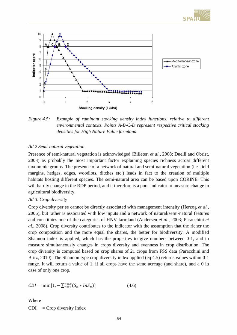
54

Figure 4.5: Example of ruminant stocking density index functions, relative to different

environmental contexts. Points A-B-C-D represent respective critical stocking densities for High Nature Value farmland

Ad 2 Semi-natural vegetation

Presence of semi-natural vegetation is acknowledged (Billeter. et al., 2008; Duelli and Obrist, 2003) as probably the most important factor explaining species richness across different taxonomic groups. The presence of a network of natural and semi-natural vegetation (i.e. field margins, hedges, edges, woodlots, ditches etc.) leads in fact to the creation of multiple habitats hosting different species. The semi-natural area can be based upon CORINE. This will hardly change in the RDP period, and it therefore is a poor indicator to measure change in agricultural biodiversity.

Ad 3. Crop diversity

Crop diversity per se cannot be directly associated with management intensity (Herzog et al., 2006), but rather is associated with low inputs and a network of natural/semi-natural features and constitutes one of the categories of HNV farmland (Andersen et al., 2003; Paracchini et al., 2008). Crop diversity contributes to the indicator with the assumption that the richer the crop composition and the more equal the shares, the better for biodiversity. A modified Shannon index is applied, which has the properties to give numbers between 0-1, and to measure simultaneously changes in crops diversity and evenness in crop distribution. The crop diversity is computed based on crop shares of 21 crops from FSS data (Paracchini and Britz, 2010). The Shannon type crop diversity index applied (eq 4.5) returns values within 0-1 range. It will return a value of 1, if all crops have the same acreage (and share), and a 0 in case of only one crop.

��I � min L1, 2 ∑ (F+ ∗ N3F++OP+O' )Q (4.6)

Where

CDI = Crop diversity Index

55

S = Share of crop (n=1,…, N)

N = number of distinguished crops

High Natural Value Index

The final index score for the arable part of the crop shares is of the crop diversity index10 (CDI) and the intensity index (Paracchini and Britz, 2010)11. The HNV farmland index is computed based on the geometric mean of the crop diversity index and the stocking density index (divided by a factor 10 to scale it to the crop diversity index).

7HE � F�I ∗ RSRSTUS � ��I ∗ US

RSTUS (4.7)

Where HNV = High Nature Value farmland index FA = Fodder acreage = Permanent grassland area CA = Arable land area

Data

Reliable data on nitrogen surplus for the period 2000 till 2009 at EU level are only available in Eurostat at NUTS0 level (and not a lower levels). Data were selected of EU25 member states that had data for the entire period. Because of the negative nitrogen surplus in Hungary in several years, Hungary was deleted. Data on GVA (Gross Value Added, is yield minus variable inputs) were from Cambridge Econometrics (CE). The CE database does not contain information on the variable inputs used in agriculture. Data on investments and labour in agriculture were also extracted from CE. The spending on measure 214 (and on Axis 1 and Axis 2) stem from CATS database. We have a balanced panel data set of 8 years (2001-2008) and 18 member states, totalling 144 observations. The data for 2000 are used to compute the change in nitrogen surplus. The change in nitrogen surplus is computed as the ratio of nitrogen surplus of the current year and previous year’s nitrogen surplus (to allow panel data estimation). The investments and spending used are the sum of current year and previous year.

The data for the HNV farmland analysis (number of livestock and acreage of crops) come from FSS (Farm Structure Survey) at NUTS2 level for 2000 and 2010. The availability of FSS data limited the number of NUTS2 regions we could use in our analysis. We have 153 regions in the dataset. For some member states we use only data at NUTS1 or NUTS0 level. Figure 4.6 shows the regions incorporated.

10 multiplied by a factor 10 to make it comparable to the stocking density index. 11 Paracchini, M. L. and W. Britz (2010) Quantifying effects of changed farm practices on biodiversity in policy impact assessment – an application of CAPRI-Spat, Ispra, Institute for Environment and Sustainability of the Joint Research Centre, European Commission, ibid. do not compute the “presence of semi-natural semi-natural vegetation”, this factor is not included in the actual index..

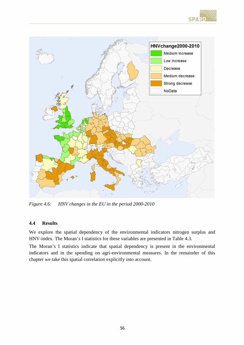
56

Figure 4.6: HNV changes in the EU in the period 2000-2010

4.4 Results

We explore the spatial dependency of the environmental indicators nitrogen surplus and HNV-index. The Moran’s I statistics for these variables are presented in Table 4.3.

The Moran’s I statistics indicate that spatial dependency is present in the environmental indicators and in the spending on agri-environmental measures. In the remainder of this chapter we take this spatial correlation explicitly into account.

57

Table 4.3 Moran’s I statistics for the environmental indicators (Nitrogen surplus and HNV-index )

2001 2009 Change between 2001-2009

Nitrogen surplus 0.516 0.290 0.368

HNV index 0.655 0.232

Spending measure 214 0.140 0.212

* All statistics in the table are statistically significant at 1%-level.

** Nitrogen surplus is three year average of nitrogen surplus (to correct for weather influences), The change in nitrogen surplus is the change between the three year average nitrogen surpluses in the beginning and end of our analysis period.

4.4.1 Nitrogen surplus

We estimate the model defined in section 4.2.3, using the Cobb-Douglas specification. Given the data presented in section 4.30 the estimated equation is below (equation 4.8). Besides the spending on RDP measure 214 (AEM) we also include the spending on RDP Axis 1 (improving the competitiveness of the agricultural and forest sector) and the spending on other measures from RDP Axis 2 (minus those on AEM). Thus we can test the impact of the interaction between different RDP-axes. Weather conditions play an important role in the yearly variation in yield, hence also in the yearly nitrogen surplus (nitrogen surplus is computed based on the actual yield per year). We add a year dummy for 2003 (variable YD) because it was an extremely dry year with low yields throughout Europe. A time trend (variable TT) is added to capture the reduction over time of the nitrogen surplus due to technological change, the related improvement of productivity and more constrained legislation. Nitrogen surplus in Eastern European countries was in the entire period much smaller than that of Western Europe (as was the yield and the input use). The productivity gap was partly closed by intensification of agriculture in Eastern European Member States, leading to higher nitrogen surpluses in the end of the RDP period. To capture this different development a dummy for the Eastern European countries (variable EE) is added.

N3HV# � �)� � �'N3"V# � ��N3$V# � �WN3�V# � �XN3G214V# � �YN3&Z1V# � �[N3&Z2V# � �\]]# ��^"�# � �_` V̀ (4.8)

For the static model we estimated different spatial panel data models. First, the random effects model (the random effects model was preferred over the fixed effects model based on the Hausman test). The diagnostic LM tests (Anselin et al., 1996) are performed on the a-spatial model to test if the error terms show a spatial structure, see (Linderhof et al., 2011) for more details. The LM-tests indicate there is scope for spatial econometrics, and that an error model is the preferred option. Second, a spatial specification for panel data was estimated in R (Millo and Piras, 2012). For the spatial panel data models the Baltagi, Song and Koh LM tests are performed (Baltagi et al., 2007). The model containing random regional effects and spatial autocorrelation was selected based on the test results.

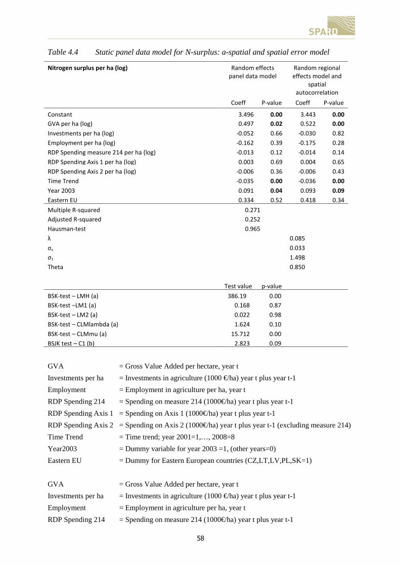
58

Table 4.4 Static panel data model for N-surplus: a-spatial and spatial error model

Nitrogen surplus per ha (log) Random effects

panel data model

Random regional

effects model and

spatial

autocorrelation

Coeff P-value Coeff P-value

Constant 3.496 0.00 3.443 0.00

GVA per ha (log) 0.497 0.02 0.522 0.00

Investments per ha (log) -0.052 0.66 -0.030 0.82

Employment per ha (log) -0.162 0.39 -0.175 0.28

RDP Spending measure 214 per ha (log) -0.013 0.12 -0.014 0.14

RDP Spending Axis 1 per ha (log) 0.003 0.69 0.004 0.65

RDP Spending Axis 2 per ha (log) -0.006 0.36 -0.006 0.43

Time Trend -0.035 0.00 -0.036 0.00

Year 2003 0.091 0.04 0.093 0.09

Eastern EU 0.334 0.52 0.418 0.34

Multiple R-squared 0.271

Adjusted R-squared 0.252

Hausman-test 0.965

λ 0.085

σν 0.033

σ1 1.498

Theta 0.850

Test value p-value

BSK-test – LMH (a) 386.19 0.00

BSK-test –LM1 (a) 0.168 0.87

BSK-test – LM2 (a) 0.022 0.98

BSK-test – CLMlambda (a) 1.624 0.10

BSK-test – CLMmu (a) 15.712 0.00

BSJK test – C1 (b) 2.823 0.09

GVA = Gross Value Added per hectare, year t

Investments per ha = Investments in agriculture (1000 €/ha) year t plus year t-1

Employment = Employment in agriculture per ha, year t

RDP Spending 214 = Spending on measure 214 (1000€/ha) year t plus year t-1

RDP Spending Axis 1 = Spending on Axis 1 (1000€/ha) year t plus year t-1

RDP Spending Axis 2 = Spending on Axis 2 (1000€/ha) year t plus year t-1 (excluding measure 214)

Time Trend = Time trend; year 2001=1,…, 2008=8

Year2003 = Dummy variable for year 2003 =1, (other years=0)

Eastern EU = Dummy for Eastern European countries (CZ,LT,LV,PL,SK=1)

GVA = Gross Value Added per hectare, year t

Investments per ha = Investments in agriculture (1000 €/ha) year t plus year t-1

Employment = Employment in agriculture per ha, year t

RDP Spending 214 = Spending on measure 214 (1000€/ha) year t plus year t-1

59

RDP Spending Axis 1 = Spending on Axis 1 (1000€/ha) year t plus year t-1

RDP Spending Axis 2 = Spending on Axis 2 (1000€/ha) year t plus year t-1 (excluding measure 214)

Time Trend = Time trend; year 2001=1,…, 2008=8

Year2003 = Dummy variable for year 2003 =1, (other years=0)

Eastern EU = Dummy for Eastern European countries (CZ,LT,LV,PL,SK=1)

First the regularity conditions are evaluated. The positive sign (significantly) for the GVA (yield minus variable inputs) per ha fits the theory that yield is positively related to N surplus. The inputs are supposed to be negatively related with nitrogen surplus (as substitutes). This is valid for both employment and investments, see Table 4.4. Investments is the summation of all farmers’ private investments (for the current year and the year before). Some investments may be related to the environment (e.g. equipment to spread manure more environmentally friendly), while others are clearly related to intensification. Spending on measure 214 is negatively related to the nitrogen surplus emission. Although the p-value is small, the coefficient is not significant. Also the other measures of Axis2 are negatively (although not significantly) related to the level of N surplus. Measure 214 and Axis2 stimulate more extensive agriculture, hence a smaller N surplus is expected. Suggesting that AEM spending stimulate a reduction of nitrogen surplus. Axis1 spending are often related to more intensified agriculture and are expected to increase N surplus. The expenditures on Axis1 show a positive (but not significant) parameter value.

The time trend has a negative sign and captures the (autonomous) reduction over time of the levels of nitrogen surplus. Due to more strict legislation farmers had already incentives to reduce their nitrogen input. This nitrogen surplus reduction over time is not seen in Eastern European countries, hence the dummy for these countries has a positive value. The year dummy for 2003 proved to be significant and has the expected positive value.

The variables that constitute nitrogen surplus are not all incorporated in the regression. Hence we have omitted variables that might be spatially related. The spatial specification, including random regional effects and spatial autocorrelation was tested to be the appropriate model. The parameter estimates are very stable when the spatial specification is added.

The dynamic version of the N surplus model explains the annual change in N surplus. The dependent variable is the log of the relative change in the impact indicator (Nsurplust/ Nsurplust-1). A reduction of N surplus gives a value smaller than 1 (and vice versa). This definition of the change in the baseline indicator prevents missing values due to the impossibility to compute logarithms of negative values. The change in baseline indicator is related to the same explanatory variables as in the ‘static’ analysis (see table 4.4) and to nitrogen surplus in the preceding year for the prescriptive aspect.

N3�HV# � �)� � �'N3HV#(' � ��N3"V# � �WN3(IV# � IV#(') � �XN3�V# � �YN3 (G214V# �G214V#(') � �[N3 (&Z1V# � &Z1V#(') � �\N3 (&Z2V# � &Z2V#(') � �^]]# � �_"�# � �')` V̀ (4.9)

60

We tested a Durbin model, in which spatially lagged variables of spending on investment and RDP measures are incorporated into our analysis (results are presented in the right hand side column of Table 4.5).

Table 4.5 Regression results of change in N-surplus (Dynamic) panel data model and Simplified Durbin model.

Change in nitrogen surplus per ha (log) One way fixed

effects model

Simplified Durbin

models


Time lag N-surplus (log) -0.671 0.00 -0.665 0.00

Spatial lag of Time lag N-surplus (log) -0.021 0.54

GVA per ha (log) 0.110 0.75 0.154 0.67

Investments per ha (log) -0.005 0.96 -0.012 0.91

Employment per ha (log) 0.082 0.81 0.056 0.88

Spending measure 214 per ha (log) -0.008 0.14 -0.008 0.16

Spatial lag Spending measure 214 per ha (log) 0.001 0.90

Spending Axis 1 per ha (log) 0.004 0.50 0.004 0.51

Spatial lag of Axis 1 per ha (log) -0.002 0.82

Spending Axis 2 (excluding M214) per ha (log) -0.004 0.39 -0.004 0.43

Spatial lag Axis 2 (excluding M214)er ha (log) 0.002 0.79

Time trend -0.018 0.12 -0.019 0.11

Year 2003 0.082 0.04 0.084 0.03

Multiple R-squared 0.407 0.412

Adjusted R-squared 0.333 0.324

Chi2

value

p-value Chi2

value

p-value

BSK-test – LMH (a) 0.090 0.62 0.003 0.73

BSK-test –LM1 (a) -0.003 1.00 -0.001 1.00

BSK-test – LM2 (a) 0.005 0.99 0.004 0.99

BSK-test – CLMlambda (a) 1.554 0.12

BSK-test – CLMmu (a) 1.305 0.19 1.086 0.28

BSJK test – C1 (b) 1.042 0.31 1.109 0.29

(a) See (Baltagi et al., 2003); (Millo and Piras, 2012) (b) See (Baltagi et al., 2007); (Millo and Piras, 2012)

61

The one way fixed effects panel data estimation provides a rather high R2 (partially due to the lagged endogenous variable) and prevents the inclusion of the Eastern European countries dummy variable. The coefficients have not changed largely compared to the ‘static’ analysis (table 4.4). The lagged nitrogen surplus parameter has a negative sign reflecting that the higher nitrogen surplus in the preceding year is, the more likely it is to be reduced. The GVA and Investments have the same sign as in the static analysis, but here it does not significantly differ from 0 (probably due to the inclusion of the time lag of nitrogen surplus). The employment variable has a counter intuitive positive sign, but this is not significant. The spending on measure 214 shows a negative parameter, and has a small p-value but does not differ significantly from 0. The spending on Axis1 and Axis2 also have the expected sign (positive for Axis1 and negative for Axis2), but also do not differ significantly from 0.

This model was tested against spatial econometric specifications using the Baltagi, Song and Koh LM tests for panel data models (Baltagi et al., 2007; Baltagi et al., 2003). None of these LM-tests indicated that a spatial model will improved the results.

The Durbin model with added spatial lagged variables of the time lag of N-surplus and of the RDP expenditures did hardly change the estimation results. None of these spatial lagged variables has an parameter estimate that differs significantly from zero. The adjusted R2 is smaller than in the model without spatial lagged variables. Again the Baltagi, Song and Koh LM tests for panel data models (Baltagi et al., 2007; Baltagi et al., 2003) show that a spatial formulation of this model is not preferred over the Durbin model.

It proved to be possible to estimate an input demand type function, relating nitrogen surplus on NUTS0 level with output, quasi fixed inputs and RDP spending in a panel data context. Both the ‘static’ and ‘dynamic’ analysis indicate in the same direction that spending on measure 214 are related to a reduction of nitrogen surplus, but the parameter estimates do not differ significantly from zero. Hence, this analysis does not prove this relation convincingly. On the other hand, all models show that parameter estimates of expenditures on axis1 have a positive sign (related to a higher nitrogen surplus) but also this relation cannot be proved.

The spatial econometric specification in the static model improves the results, indicating that the omitted variables show spatial correlation. We hardly expect any significant spill-overs at NUTS0 level. In the dynamic model, a spatial specification did not add to the model. This is probably due to the incorporation of the time lag of nitrogen surplus, this will capture part of the omitted variables from the static analysis.

4.4.2 High Natural Value Farmland

We use the HNV farmland index as dependent variable, as proxy for agricultural biodiversity; see 4.2.3. In this section we focus on the relation between HNV and measure 214, but also other measures will influence the farmer’s decisions or affect the region. Measures in axis 1 will stimulate intensification of production, while axis 2 measures are meant to reverse intensification or to maintain existing production systems. To take account of the impact of these measures on the impact indicators the spending on axis1 and axis2 are also included in the econometric analysis. This results in equation 4.10.

62

7HE# � �)� � �' � �� N3"# � �W (N3∑'# I#) � �X N3�V � �Y (N3∑'# G214#) � �[ (N3∑'# &Z1#) ��\ (N3∑'# &Z2#) � �^ ab# � �_ N3Fc# (4.10)

This index lies between 0 and 1. For agricultural biodiversity we expect a decreasing marginal rate of substitution (a positive relation between this indicator and the inputs and a negative relation with the marketable outputs). We do not know the actual relation between the HNV index and the level of agricultural biodiversity, but expect that due to the relevant trajectory of this variable between 0 and 1, the index is linearly related to the logs of the explanatory variables. We use the Cobb-Douglas specification (eq 4.10), because it allows for decreasing marginal returns.

The HNV-index is a combination of the livestock density index and crop diversity index and based upon the farm structure in the region. We first estimate the ‘static’ model for 2010 to present the relation between the level of the impact indicator and the explanatory variables. These explanatory variables are determined by the production function. We do not use explanatory variables from the FSS, because the dependent variable HNV is already constructed from FSS-variables (as in section 3). We want to avoid a tautological estimation. The size of the regions (in logarithms) is tested as an explanatory variable because the crop index is influenced by this size (larger regions are more likely to have a more diverse array of crops). Also the percentage of agricultural land that does not belong to the categories grassland and arable land is used, because information of this land category is not incorporated in the HNV index. Thereafter we estimate the dynamic version, relating the dependent variable HNV-index in 2010 to HNV-index in 2000, the summation over the entire period of the private investments and the spending in AEM, Axis1 and Axis2 the other explanatory variables are the same as in the ‘static’ model. The Gabriel weight matrix, see Figure 2.2.

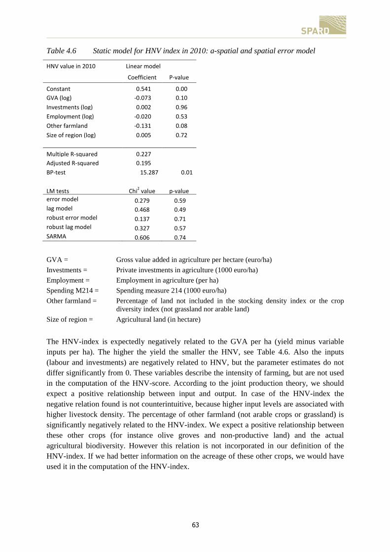
63

Table 4.6 Static model for HNV index in 2010: a-spatial and spatial error model

HNV value in 2010 Linear model

Coefficient P-value

Constant 0.541 0.00

GVA (log) -0.073 0.10

Investments (log) 0.002 0.96

Employment (log) -0.020 0.53

Other farmland -0.131 0.08

Size of region (log) 0.005 0.72

Multiple R-squared 0.227

Adjusted R-squared 0.195

BP-test 15.287 0.01

LM tests Chi2 value p-value

error model 0.279 0.59

lag model 0.468 0.49

robust error model 0.137 0.71

robust lag model 0.327 0.57

SARMA 0.606 0.74

GVA = Gross value added in agriculture per hectare (euro/ha)

Investments = Private investments in agriculture (1000 euro/ha)

Employment = Employment in agriculture (per ha)

Spending M214 = Spending measure 214 (1000 euro/ha)

Other farmland = Percentage of land not included in the stocking density index or the crop diversity index (not grassland nor arable land)

Size of region = Agricultural land (in hectare)

The HNV-index is expectedly negatively related to the GVA per ha (yield minus variable inputs per ha). The higher the yield the smaller the HNV, see Table 4.6. Also the inputs (labour and investments) are negatively related to HNV, but the parameter estimates do not differ significantly from 0. These variables describe the intensity of farming, but are not used in the computation of the HNV-score. According to the joint production theory, we should expect a positive relationship between input and output. In case of the HNV-index the negative relation found is not counterintuitive, because higher input levels are associated with higher livestock density. The percentage of other farmland (not arable crops or grassland) is significantly negatively related to the HNV-index. We expect a positive relationship between these other crops (for instance olive groves and non-productive land) and the actual agricultural biodiversity. However this relation is not incorporated in our definition of the HNV-index. If we had better information on the acreage of these other crops, we would have used it in the computation of the HNV-index.

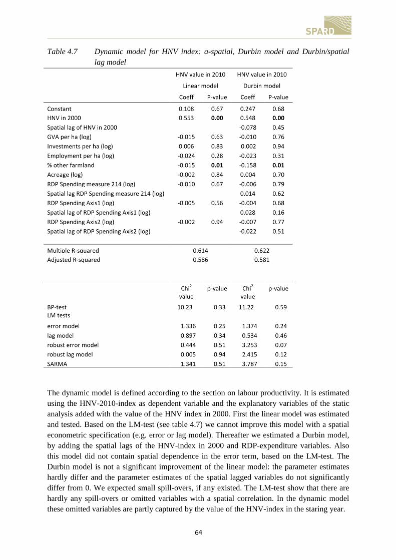
64

Table 4.7 Dynamic model for HNV index: a-spatial, Durbin model and Durbin/spatial lag model

HNV value in 2010

Linear model

HNV value in 2010

Durbin model


Constant 0.108 0.67 0.247 0.68

HNV in 2000 0.553 0.00 0.548 0.00

Spatial lag of HNV in 2000 -0.078 0.45

GVA per ha (log) -0.015 0.63 -0.010 0.76

Investments per ha (log) 0.006 0.83 0.002 0.94

Employment per ha (log) -0.024 0.28 -0.023 0.31

% other farmland -0.015 0.01 -0.158 0.01

Acreage (log) -0.002 0.84 0.004 0.70

RDP Spending measure 214 (log) -0.010 0.67 -0.006 0.79

Spatial lag RDP Spending measure 214 (log) 0.014 0.62

RDP Spending Axis1 (log) -0.005 0.56 -0.004 0.68

Spatial lag of RDP Spending Axis1 (log) 0.028 0.16

RDP Spending Axis2 (log) -0.002 0.94 -0.007 0.77

Spatial lag of RDP Spending Axis2 (log) -0.022 0.51

Multiple R-squared 0.614 0.622

Adjusted R-squared 0.586 0.581

Chi2

value

p-value Chi2

value

p-value

BP-test 10.23 0.33 11.22 0.59

LM tests

error model 1.336 0.25 1.374 0.24

lag model 0.897 0.34 0.534 0.46

robust error model 0.444 0.51 3.253 0.07

robust lag model 0.005 0.94 2.415 0.12

SARMA 1.341 0.51 3.787 0.15

The dynamic model is defined according to the section on labour productivity. It is estimated using the HNV-2010-index as dependent variable and the explanatory variables of the static analysis added with the value of the HNV index in 2000. First the linear model was estimated and tested. Based on the LM-test (see table 4.7) we cannot improve this model with a spatial econometric specification (e.g. error or lag model). Thereafter we estimated a Durbin model, by adding the spatial lags of the HNV-index in 2000 and RDP-expenditure variables. Also this model did not contain spatial dependence in the error term, based on the LM-test. The Durbin model is not a significant improvement of the linear model: the parameter estimates hardly differ and the parameter estimates of the spatial lagged variables do not significantly differ from 0. We expected small spill-overs, if any existed. The LM-test show that there are hardly any spill-overs or omitted variables with a spatial correlation. In the dynamic model these omitted variables are partly captured by the value of the HNV-index in the staring year.

65

Expectedly, the incorporation of the HNV-index in the starting year as explanatory variables gives a much higher R2 than in the static analysis, see Table 4.7. In the dynamic models this HNV-index 2000 is positively related to the HNV-index in 2010. The coefficients for GVA and investments have the appropriate signs (although not significantly differing from 0). The percentage of other land is negatively (and significantly) related to HNV-index. The RDP spending (AEM, axis1, axis2) are all negatively related to the HNV-index in the linear model. For AEM and Axis2, this is not according to the theory, however the parameter estimates do not differ significantly from 0.

Conclusions The HNV index can be used in the analysis of the impact of AEM. The R2 in the static model is not large, reflecting that we did not incorporate all relevant explanatory variables. The omitted variables could be partly compensated for using the spatial error model. The negative parameter estimate for the percentage of other land is an indication that our constructed HNV-index has to be improved upon to be able to reflect the actual rate of biodiversity better. The dynamic model does not provide an entirely different picture. The spending on AEM are negatively related to HNV-index in the linear model, but if we apply spatial specifications this relationship turn out to be positive (as expected).


In this chapter we demonstrated that it is possible to relate the spending on measure 214 (Agri-environmental measures) EU wide to changes in selected CMEF baseline indicators, although we used some simplifications to create EU wide baseline indicators. Although the underlying physical (environmental) system shows clear spillover effects of water quality and (agricultural) biodiversity, the actual baseline indicators selected and elaborated for our analysis will not show these spillover effects. Measure 214 consists of an array of different measures, that all affect the environment differently. The actual combination of specific measures will differ between regions, as will the impact of these measures on either nitrogen surplus or HNV. Spending on measure 214 is relatively small combined to other transactions in rural areas and other policies that influences farmers’ behaviour with respect to the environment (e.g. Nitrate directive, Water Framework Directive). Especially at an aggregated area (as NUTS0) we do not expect to find these measures to affect the baseline indicators significantly. We analysed the baseline indicators at a level, at which we do not expect to find significant spillovers. The main spatial effect captured in our spatial econometric analysis is the spatial relation in the omitted variables. Dealing with environmental processes an array of omitted variables exists due to missing data (or missing indicators to aggregate these data to the relevant level of analysis), examples are the weather and climate, soil type. These omitted variables are clearly spatially correlated and their effect on the impact indicator can be captured by spatial econometrics (as done in this chapter).

Based on the estimation results we can conclude that spending on measure 214 affect their impact indicators in the expected direction, but this relation could not be tested significantly. For nitrogen surplus all models point in the same direction that AEM are related to a reduction of N surplus and the related improvement of water quality. Evidence for impact on the HNV-index is less strong. We also found indications that the HNV-index constructed for

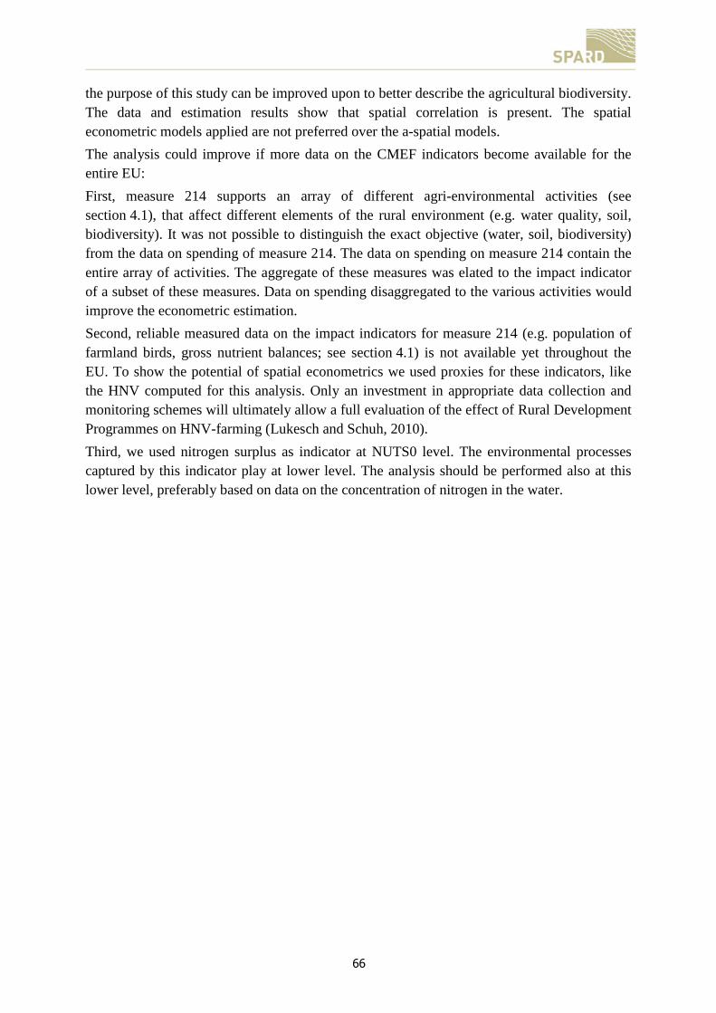
66

the purpose of this study can be improved upon to better describe the agricultural biodiversity. The data and estimation results show that spatial correlation is present. The spatial econometric models applied are not preferred over the a-spatial models.

The analysis could improve if more data on the CMEF indicators become available for the entire EU:

First, measure 214 supports an array of different agri-environmental activities (see section 4.1), that affect different elements of the rural environment (e.g. water quality, soil, biodiversity). It was not possible to distinguish the exact objective (water, soil, biodiversity) from the data on spending of measure 214. The data on spending on measure 214 contain the entire array of activities. The aggregate of these measures was elated to the impact indicator of a subset of these measures. Data on spending disaggregated to the various activities would improve the econometric estimation.

Second, reliable measured data on the impact indicators for measure 214 (e.g. population of farmland birds, gross nutrient balances; see section 4.1) is not available yet throughout the EU. To show the potential of spatial econometrics we used proxies for these indicators, like the HNV computed for this analysis. Only an investment in appropriate data collection and monitoring schemes will ultimately allow a full evaluation of the effect of Rural Development Programmes on HNV-farming (Lukesch and Schuh, 2010).

Third, we used nitrogen surplus as indicator at NUTS0 level. The environmental processes captured by this indicator play at lower level. The analysis should be performed also at this lower level, preferably based on data on the concentration of nitrogen in the water.

67

5 Tourism

5.1 Introduction

From Axis 3, we explore a spatial analysis for measures that are primarily focused on the improvement of non-agriculture activities in rural areas. Examples are the measures “diversification into non-agricultural activities” by farmers including agro-tourism (RDP measure 311) and “encouraging tourism” in rural areas (RDP measure 313). Measures in Axis 3 can thus be described as true rural (rather than agricultural) development measures of the RD catalogue (Agra, 2005). The content and the grants for measure 311 are similar to measure 121 with the difference that measure 311 focuses on non-agricultural investments by farmers, while 121 has a pure agricultural focus. For measure 313 there is no specific target group. Both measures were handled together in the programming period 2000-2006, and a separation of the evaluation results only for non-agricultural investments is factually not possible (Uthes et al., 2011).

Table 5.1 Axis 3 EU spending on measures 311 and 313.

Measure 2000-2006 2007-2013

€ mln % € mln %

311 Diversification of agricultural activities (Art 33) 645 12.2 1,301 8.6

313 Encouragement for tourist and craft activities (Art

33, 2000-06) / tourism activities (2007-)

433 8.2 1,165 7.7

Total Axis 3 5,273 100 15,066 100

Note: Data for Germany, Spain, UK, Italy, Portugal and Malta were not yet included in the period 2007-2013. Source: (Dwyer et al., 2008)

The spending on measures 311 and 313 is increasing over the last years, see Table 5.1. In 2007, about €12 million was spent on measure 311 and it increased to almost €200 million in 2010. For measure 313, we observed a similar pattern; €6 million in 2007 and €157 million in 2010. The spending on either measure 311 or 313 also show a huge difference across EU Member States. The maps in Figure 5.3 and Figure 5.4 show the spending on measure 311 and 313 at NUTS2 level in 2010.

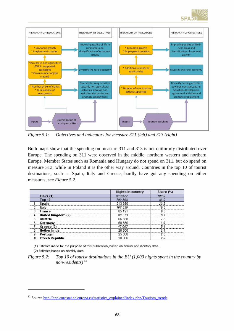
68

Figure 5.1: Objectives and indicators for measure 311 (left) and 313 (right)

Both maps show that the spending on measure 311 and 313 is not uniformly distributed over Europe. The spending on 311 were observed in the middle, northern western and northern Europe. Member States such as Romania and Hungary do not spend on 311, but do spend on measure 313, while in Poland it is the other way around. Countries in the top 10 of tourist destinations, such as Spain, Italy and Greece, hardly have got any spending on either measures, see Figure 5.2.

Figure 5.2: Top 10 of tourist destinations in the EU (1,000 nights spent in the country by

non-residents) 12

12 Source http://epp.eurostat.ec.europa.eu/statistics_explained/index.php/Tourism_trends

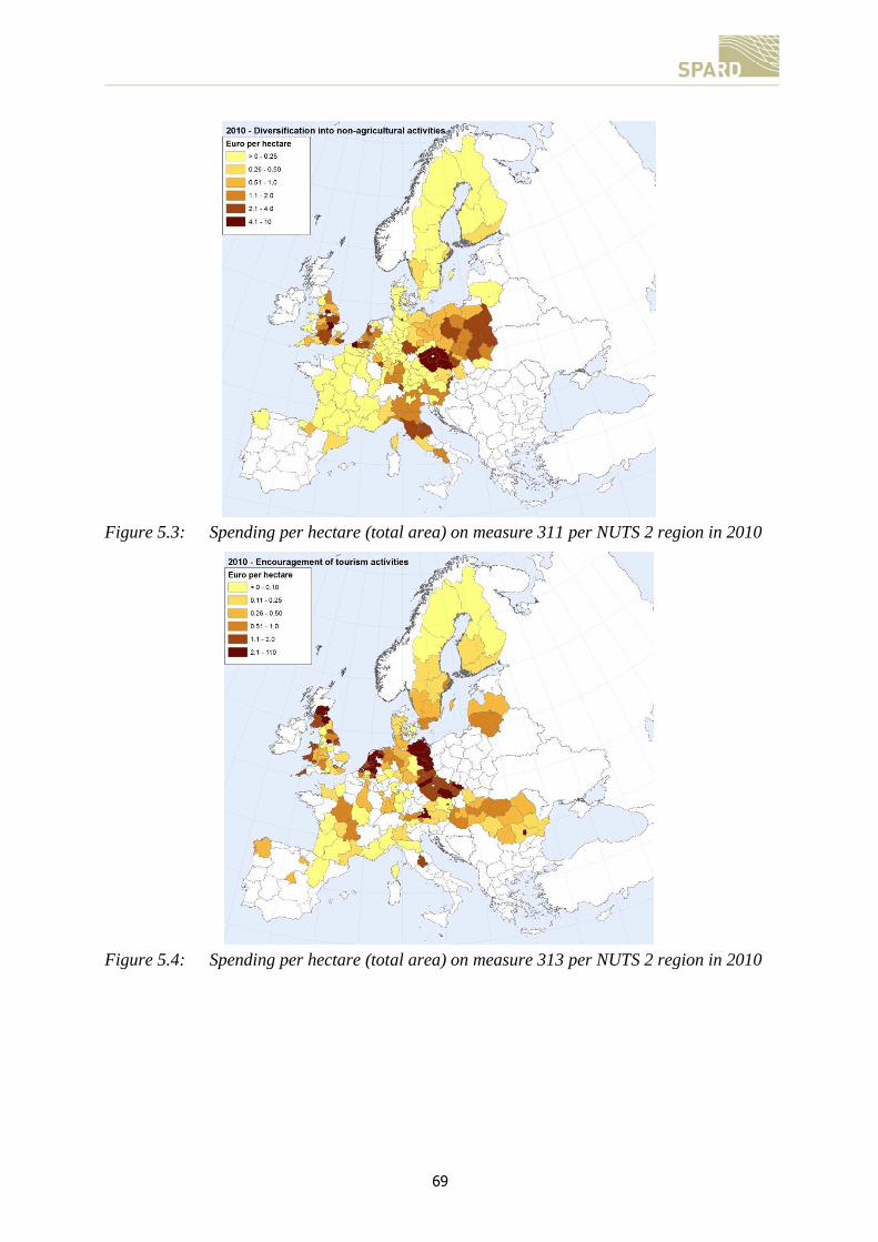
69

Figure 5.3: Spending per hectare (total area) on measure 311 per NUTS 2 region in 2010

Figure 5.4: Spending per hectare (total area) on measure 313 per NUTS 2 region in 2010

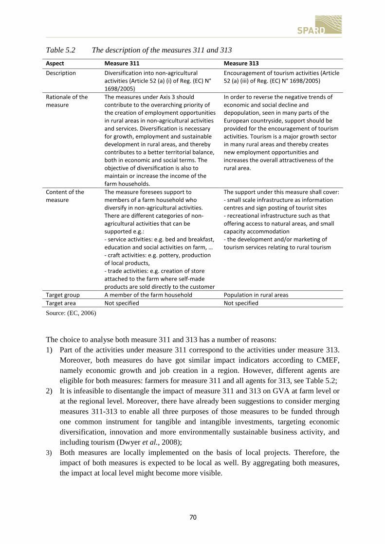
70

Table 5.2 The description of the measures 311 and 313

Aspect Measure 311 Measure 313

Description Diversification into non-agricultural

activities (Article 52 (a) (i) of Reg. (EC) N°

1698/2005)

Encouragement of tourism activities (Article

52 (a) (iii) of Reg. (EC) N° 1698/2005)

Rationale of the

measure

The measures under Axis 3 should

contribute to the overarching priority of

the creation of employment opportunities

in rural areas in non-agricultural activities

and services. Diversification is necessary

for growth, employment and sustainable

development in rural areas, and thereby

contributes to a better territorial balance,

both in economic and social terms. The

objective of diversification is also to

maintain or increase the income of the

farm households.

In order to reverse the negative trends of

economic and social decline and

depopulation, seen in many parts of the

European countryside, support should be

provided for the encouragement of tourism

activities. Tourism is a major growth sector

in many rural areas and thereby creates

new employment opportunities and

increases the overall attractiveness of the

rural area.

Content of the

measure

The measure foresees support to

members of a farm household who

diversify in non-agricultural activities.

There are different categories of non-

agricultural activities that can be

supported e.g.:

- service activities: e.g. bed and breakfast,

education and social activities on farm, …

- craft activities: e.g. pottery, production

of local products,

- trade activities: e.g. creation of store

attached to the farm where self-made

products are sold directly to the customer

The support under this measure shall cover:

- small scale infrastructure as information

centres and sign posting of tourist sites

- recreational infrastructure such as that

offering access to natural areas, and small

capacity accommodation

- the development and/or marketing of

tourism services relating to rural tourism

Target group A member of the farm household Population in rural areas

Target area Not specified Not specified

Source: (EC, 2006)

The choice to analyse both measure 311 and 313 has a number of reasons: 1) Part of the activities under measure 311 correspond to the activities under measure 313.

Moreover, both measures do have got similar impact indicators according to CMEF, namely economic growth and job creation in a region. However, different agents are eligible for both measures: farmers for measure 311 and all agents for 313, see Table 5.2;

2) It is infeasible to disentangle the impact of measure 311 and 313 on GVA at farm level or at the regional level. Moreover, there have already been suggestions to consider merging measures 311-313 to enable all three purposes of those measures to be funded through one common instrument for tangible and intangible investments, targeting economic diversification, innovation and more environmentally sustainable business activity, and including tourism (Dwyer et al., 2008);

3) Both measures are locally implemented on the basis of local projects. Therefore, the impact of both measures is expected to be local as well. By aggregating both measures, the impact at local level might become more visible.

71

As mentioned in Figure 5.1, the impact indicators of the measures 311 and 313 are economic growth and employment creation. However, those indicators are rather generic impact indicators in CMEF and it is very difficult to disentangle impacts of specific measures, Therefore, we focus our spatial analysis on one of the result indicators namely tourism, so that we are able to disentangle the impact of specific measures. For measure 313, the number of tourist visits is defined as a result indicator, see Figure 5.1. For this reason, Eurostat collects data on the number of nights spent, where a sub-selection for non-residents is available as well. For measure 311, this is not an explicit result indicator, but an optional one, since Bed & Breakfast activities are explicitly defined in the CMEF description of measure 311 (EC, 2006).

The outline of this Chapter is as follows. Section 5.2 discusses the econometric specification of the tourism analysis. Then Section 5.3 defines the indicators and presents the data used. In Section 5.4, the estimation procedure and results are presented. Finally, Section 5.5 discusses the results and the conclusions from using spatial econometric analysis to explain the impact of measure 313 on development of tourism.


5.2.1 Introduction

The rationale of measures 311 and 313 is the economic growth of a rural area by encouraging rural tourism in the EU regions. In fact, measure 311 supports farmers that would like to start tourism activities next to their agricultural activities, and measure 313 stimulates the increase of tourist demand in a region for a wide range of applicants. In the economic literature, there is a wide range of articles on tourism and its impact on the economy. Tourism can be helpful in improving the multi-functionality of the a region which implies more robust economic development (van Leeuwen et al., 2009). In addition, stimulating tourism in a region also implies an increase in employment, because tourism is a rather labour-intensive sector but it does not require highly skilled labour, see (van Leeuwen et al., 2009).

In the literature, tourism has been analysed from many different perspectives: (i) production efficiency, (ii) impact of tourism on the economy and (iii) growth-led economy for tourism. The production efficiency perspective relates to the efficient use of tourism accommodations (Bernini and Guizzardi, 2010). They for instance analyse hotel efficiency in Italy in order to identify the causes of the low hotel efficiency growth compared to France and Spain. This type of analyses is beyond the scope of SPARD.

The studies on the importance of tourism on the (local, regional or national) economy mainly use input-output tables and multiplier analyses (van Leeuwen et al., 2009). They summarize a number of studies that analyse the relevance of tourism on the regional economy from a static perspective. Most studies used input-output tables over time in order to derive multiplier impacts on the economy due to changes in tourism. In addition, other studies explore a computable general equilibrium model for analysing changes in the drivers of tourism (Dwyer et al., 2004). Studies using CGE models are useful for ex-ante evaluation of tourism, but they do not provide evidence for new drivers of tourism, because drivers are predefined in CGE models.

72

Finally, there is also a stream of articles on the analyses of tourist demand and the role of tourism in the so-called growth-led economy. In growth-led economy, tourism is one of the drivers of economic growth. The role of tourism in the economy is analysed with models based on the economic growth theory using time series or panel data analyses. Different studies found that: tourism-based economies have higher economic growth rates than non-tourism based economies (Brau et al., 2004; Brau et al., 2007); there is evidence for positive unidirectional causality from real GDP to international tourism revenues (Payne and Mervar, 2010), which supports the economic-driven tourism growth hypothesis; and tourism stimulates the local firms’ productivity and creates new job opportunities that increase the country’s welfare (Nissan et al., 2011).

Goel and Budak (2010) analysed more specifically different aspects of tourism on economic growth, and they found that strengthened tourism safety regulations (avoiding negative events (Yang and Wong, 2012)) and government’s prioritization of tourism boost economic growth, while tourism initiatives and infrastructure investments seem to have opposite effects. If the impacts of all aspects are summed up, economic growth is higher in countries that transform from agricultural based to service based economies (Goel and Budak, 2010). A 150 countries comparison provided empirical evidence that tourism-based economies did not grow at a higher rate than non-tourism-based countries since the 1990s (Figini and Vici, 2010).

Tourism demand is often analysed with a temporal perspective (Morley, 2009). The specification of a tourism demand model now commonly includes lagged demand as an explanatory variable. This raises issues in the formulation and interpretation of econometric tourism demand models. He also argued that a simple lagged demand term is not sufficient to account for the dynamics of tourism demand. The dynamics of tourism demand have spatial aspect as well (Morley, 2009).

Marrocu and Paci (2011) examine tourism flows as determinants of regional total factor productivity within a spatial framework. Within their analysis of 199 European regions, they controlled for intangible factors, such as human, social and technological capital, and for the degree of accessibility (Marrocu and Paci, 2011). Their empirical results showed that tourism flows enhance spatial spillovers have positive impacts on regional economic growth.

5.2.2 Spillover effects

Spillover effects in tourism reflect indirect or unintentional effects of a region’s tourism industry due to tourism flows to other regions (Yang and Wong, 2012). As a result, tourism in a region can benefit (or suffer) from regional tourism developments in their neighbouring regions. Yang and Wong (2012) discussed 7 types of spillover effects: one at the demand side (multiple destination spillovers or in other words round trips like cruises), and six supply side spillovers (labour movement, demonstration effect, competition effect, market access spillovers, joint promotion, and negative external events) in the case of city tourism.

For our analysis, we explore the applicability of the different types of spillovers and formulate hypotheses for our regional tourism analysis, see Table 5.3. In particular, we distinguish between inbound and domestic tourism. We ignore multiple destination spillovers, because we do not take into account the origin of tourists in our analyse. Labour movement means that

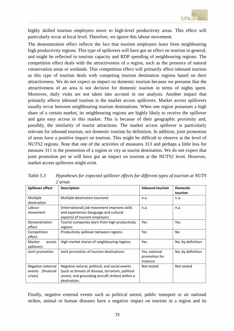
73

highly skilled tourism employers move to high-level productivity areas. This effect will particularly occur at local level. Therefore, we ignore this labour movement.

The demonstration effect reflects the fact that tourism employers learn from neighbouring high productivity regions. This type of spillovers will have got an effect on tourism in general, and might be reflected in tourism capacity and RDP spending of neighbouring regions. The competition effect deals with the attractiveness of a region, such as the presence of natural conservation areas or wetlands. This competition effect will primarily affect inbound tourism as this type of tourism deals with competing tourism destination regions based on their attractiveness. We do not expect an impact on domestic tourism because we presume that the attractiveness of an area is not decisive for domestic tourism in terms of nights spent. Moreover, daily visits are not taken into account in our analysis. Another impact that primarily affects inbound tourism is the market access spillovers. Market access spillovers usually occur between neighbouring tourism destinations. When one region possesses a high share of a certain market, its neighbouring regions are highly likely to receive the spillover and gain easy access to this market. This is because of their geographic proximity and, possibly, the similarity of tourist attractions. The market access spillover is particularly relevant for inbound tourism, not domestic tourism by definition. In addition, joint promotion of areas have a positive impact on tourism. This might be difficult to observe at the level of NUTS2 regions. Note that one of the activities of measures 313 and perhaps a little less for measure 311 is the promotion of a region or city as tourist destination. We do not expect that joint promotion per se will have got an impact on tourism at the NUTS2 level. However, market access spillovers might exist.

Table 5.3 Hypotheses for expected spillover effects for different types of tourism at NUTS 2 areas

Spillover effect Description Inbound tourism Domestic

tourism

Multiple

destination

Multiple destination tourisme n.a. n.a.

Labour

movement

(International) job movement improves skills

and experiences (language and cultural

aspects) of tourism employers

n.a. n.a.

Demonstration

effect

Tourist companies learn from high productivity

regions

Yes Yes

Competition

effect.

Productivity spillover between regions. Yes No

Market access

spillovers

High market shares of neighbouring regions. Yes No, by definition

Joint promotion Joint promotion of tourism destinations Yes, national

promotion for

instance

No, by definition

Negative external

events (financial

crises)

Negative natural, political, and social events

(such as threats of disease, terrorism, political

unrest, and grounding aircraft strikes) within a

destination.

Not tested Not tested

Finally, negative external events such as political unrest, public transport or air national strikes, animal or human diseases have a negative impact on tourism in a region and its

74

neighbouring regions. In the last decade, a number of negative external effects have occurred, such as increased risk of terrorism attacks, grounding aircraft strikes and threatening diseases, so these spillover effects might be present. However, there are no good indicators available for those events to include in our empirical analyses, and we will not be able to test the hypothesis of the presence of spillovers of negative events.

In summary, we will test the presence of three types of spillovers. The demonstration effect will be related to the RDP spending for the stimulation of tourism. The competition and market access will be related to the capacity of tourism. This means that we will not be able to distinguish between competition and market access spillovers.

5.2.3 Model

For the assessment of the impact of RDP measures 311 and 313, we start with a suitable two equation model from the literature (Nissan et al., 2011):

( ) ε+= TOURKHUIPEfGDP ,,, (5.1)

( ) ν+= MSGDPTEAhTOUR ,, (5.2)

Regional gross domestic product (GDP) is explained by the factor capital proxied by public expenditures (PE) and the private investment (I), the factor labour proxied by human capital (KHU) and an indicator for the tourism sector (TOUR). Tourism is endogenous itself, and is explained by total entrepreneurship activity (TEA) which is a combined proxy for the factors capital and labour, GDP and the money supply (MS). Nissan et al. (2011) use panel data for the estimation of both equations so that they take into account temporal dependencies but they ignore spatial dependencies.

Table 5.3 shows that we do expect spillovers in the case of tourism assessment. Moreover, there are two additional reasons to take into account spatial dependencies in tourism. The maps in Figure 5.3 and Figure 5.4 in the previous section showed that the spending on both measures is not uniformly distributed over the NUTS2 regions. Also, spatial data analysis of tourism indicators did show significant spatial dependencies, see section 5.4 later on. Ignoring the spatial dependencies might lead to biased estimators. Therefore, we start simple with the exploration of the tourism model in Eq. (5.2) in order to be able to take into account the spatial dependencies in a proper way.

In addition to the tourism model of Nissal et al. (2011), our literature survey yields a number of relevant explanatory variables. As a result, we specify our preferred specification of tourism in a region as follows:

ν+= ),,,,,,( RDPCliAccNatEnvEconDemCaphTOUR (5.3)

Instead of including a combined factor for entrepreneurship, we use separate variables for capital and labour. The variable Cap is the capacity of tourist accommodations which is a proxy for capital in 5.3, Dem represents the demographic variables which is a proxy for labour factor in Eq. 5.3. Econ refers to economic indicators of the region, Unempl is the

75

unemployment rate, NatEnv is the set of natural environment variables, Acc is the set of accessibility variables like the presence of infrastructure and Cli are a set of climate variables (precipitation, temperature etc.). In addition, the spending on RDP measures (RDP) will be included as well.

Preferably, we would like to include all relevant variables in the analysis, but due to limited data availability not all variables are available for all NUTS2 regions at the EU27 level. The capacity is the number of bed places per region which are available the whole year, and the changes of capacity over time is a proxy of the investments in the tourism sector in the region. This variable is divided into capacity for hotels and holiday houses. The demographic variables include population density and the size of the area to indicate the urbanisation of the region. GDP (Gross domestic product) and the unemployment rate indicate the wealth level of the region. Unfortunately, the GDP variable highly correlates with population density, and therefore we decided to neglect GDP in our analysis. The NatEnv variables are variables like the share of forest or other natural areas, the share of wetlands and the presence of beaches. Acc variables include the infrastructure of a region including roads network, presence of harbours and airports for instance. Cli variables would include the climatic variables, such as precipitation, number of sunny days in Summer and temperature in Summer. Unfortunately, suitable climate indicators for all NUTS2 in the EU27 are no readily available. Below, we take into account indicators of the different characteristics in Eq. (5.3) which are readily available from Eurostat and other public sources.


The econometric specification in the previous section is estimated with data at the level of NUTS2 regions. In terms of CMEF, we prefer to use impact indicators such as economic growth or employment creation. Those indicators are rather generic, so we selected one of the CMEF result indicators for our assessment which is the increase in the number of visitors, see also Section 5.2.

In CMEF, there is preference for the distinction between visitors staying overnight and daily visitors. However, the tourist data from Eurostat includes information on nights spent by tourists, and not on daily visitors. Moreover, Eurostat makes two distinction in their tourism data which are relevant to take into account in our spatial analysis. First, Eurostat distinguishes between inbound (or incoming) tourism and domestic tourism. Inbound tourism means tourists living outside the region that stay at least one night in the region. Domestic tourism are inhabitants of the region which spent at least one night in any type of collective accommodation. Secondly, Eurostat distinguishes two types of collective accommodations.

According to the definition of Eurostat, a collective tourist accommodation establishment is an accommodation establishment providing overnight lodging for the traveller in a room or some other unit, with the number of places provided greater than a specified minimum for groups of persons exceeding a single family unit. In addition, all the places in the establishment must come under a common commercial-type management, even if the establishment is non-profit-making.

The collective tourist accommodation establishments includes two categories (see http://epp.eurostat.ec.europa.eu/cache/ITY_SDDS/en/tour_cap_esms.htm for the definition:

1. “hotels and similar establishments” referred to as hotels

76

2. “other collective accommodation establishments such as holiday dwellings, tourist campsites, marinas; and specialised establishments such as health establishments, work and holiday camps, public means of transport and conference centres” referred to as holiday houses

From the Eurostat data, we have derived four indicators which we will distinguish in our analyse data from out four types of tourist namely:

• Inbound tourism in hotels: the number of nights spent in hotels and similar collective accommodations by non-residents.

• Inbound tourism in holiday houses and camping sites: the number of nights spent in other collective accommodations (incl. holiday houses and camping sites) by non-residents.

• Domestic tourism in hotels: the number of nights spent in hotels and similar collective accommodations by residents.

• Domestic tourism in holiday houses and camping sites: the number of nights spent in other collective accommodations (incl. holiday houses and camping sites) by residents.

Note that the four indicators divide tourism into four mutually exclusive groups of tourism. Furthermore, the four types of indicators can also be different in the number of tourist and the duration of their stay. However, we have no information on those items.

For our analyses, we use the nights spent in tourist collective accommodation establishments in the years 2001 and 2009 at NUTS2 level. The emphasis of our analyses is twofold:

• What is the impact of RDP spending on the encouragement of tourism? • Which spillovers are there in the analysis of tourism, and more specifically do the RDP

expenditures entail spillover effect?

Eurostat presents the data at NUTS2 level, but the indicators are not available for all NUTS2 areas. Therefore, we constructed a sample of NUTS2 areas based on the following criteria:

• Availability of tourist data at NUTS2 level, which means that NUTS2 areas in Ireland, Inner London, Outer London are excluded, because data are lacking.

• Overseas areas of France, Portugal, Spain and the Netherlands are excluded, see the paragraph on the weight matrix.

• European Island are excluded as well. This is due to our choice of our weighing matrix, see below. For many Islands, tourism is an important economic activity, but we have to exclude them in order to be able to explore spatial econometric analyses.

When we take a look at the tourist data at NUTS2 level, the information is not always available for the years 2001 and 2009. For cases with missing tourism information, we first used imputed data for 2001 based on average numbers in the period 2000 and 2002 and for 2009 based on average numbers in the period 2008-2010. In this way, we do not have to exclude all the NUTS2 areas without data on tourism for the year 2009. Our final sample included 251 NUTS2 areas.

Variables

We already listerd our variables in Section 5.2.3. Ideally, the origin of the tourist could be of relevance to estimate the demand for tourism, however there are no data available – at least not to our knowledge – on the origin of tourists at the EU27 level. Finally, we include country

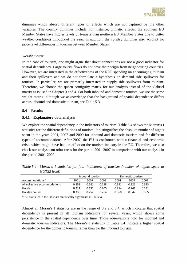
77

dummies which absorb different types of effects which are not captured by the other variables. The country dummies include, for instance, climatic effects: the southern EU Member States have higher levels of tourists than northern EU Member States due to better weather conditions throughout the year. In addition, the country dummies also account for price level differences in tourism between Member States.

Weight matrix

In the case of tourism, one might argue that direct connections are not a good indicator for spatial dependency. Large tourist flows do not have their origin from neighbouring countries. However, we are interested in the effectiveness of the RDP spending on encouraging tourism and their spillovers and we do not formulate a hypothesis on demand side spillovers for tourism. In particular, we are primarily interested in supply side spillovers from tourism. Therefore, we choose the queen contiguity matrix for our analysis instead of the Gabriel matrix as is used in Chapter 3 and 4. For both inbound and domestic tourism, we use the same weight matrix, although we acknowledge that the background of spatial dependence differs across inbound and domestic tourism, see Table 5.3.

5.4 Results

5.4.1 Explanatory data analysis

We explore the spatial dependency in the indicators of tourism. Table 5.4 shows the Moran’s I statistics for the different definitions of tourism. It distinguishes the absolute number of nights spent in the years 2001, 2007 and 2009 for inbound and domestic tourism and for different types of accommodations. After 2007, the EU is confronted with a financial and economic crisis which might have had an effect on the tourism industry in the EU. Therefore, we also check our analysis on robustness for the period 2001-2007 in comparison with our analysis in the period 2001-2009.

Table 5.4 Moran’s I statistics for four indicators of tourism (number of nights spent at NUTS2 level)

Inbound tourism Domestic tourism

Accommodations * 2001 2007 2009 2001 2007 2009

All collective accommodations 0.258 0.241 0.258 0.381 0.321 0.333 Hotels 0.211 0.191 0.205 0.254 0.241 0.231 Holiday houses 0.335 0.252 0.264 0.360 0.347 0.355

* All statistics in the table are statistically significant at 1%-level.

Almost all Moran’s I statistics are in the range of 0.2 and 0.4, which indicates that spatial dependency is present in all tourism indicators for several years, which shows some persistence in the spatial dependence over time. Those observations hold for inbound and domestic tourism indicators. The Moran’s I statistics in Table 5.4 indicate a higher spatial dependence for the domestic tourism rather than for the inbound tourism.

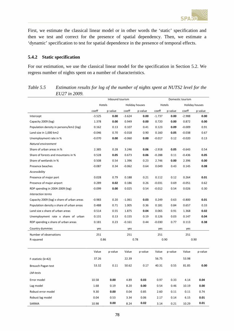
78

First, we estimate the classical linear model or in other words the ‘static’ specification and then we test and correct for the presence of spatial dependency. Then, we estimate a ‘dynamic’ specification to test for spatial dependence in the presence of temporal effects.

5.4.2 Static specification

For our estimation, we use the classical linear model for the specification in Section 5.2. We regress number of nights spent on a number of characteristics.

Table 5.5 Estimation results for log of the number of nights spent at NUTS2 level for the EU27 in 2009.


Hotels Holiday houses Hotels Holiday houses

coeff p-value coeff p-value coeff p-value coeff p-value

Intercept -3.525 0.00 -3.624 0.00 -1.737 0.00 -2.988 0.00

Capacity 2009 (log) 1.378 0.00 0.949 0.00 0.720 0.00 0.872 0.00

Population density in persons/km2 (log) 0.162 0.13 0.107 0.41 0.123 0.09 -0.009 0.91

Land size in 1,000 km2 -0.046 0.70 -0.018 0.90 0.160 0.05 -0.038 0.67

Unemployment rate in % -0.070 0.00 -0.060 0.00 -0.017 0.12 -0.020 0.13

Natural environment

Share of urban areas in % 2.385 0.28 3.246 0.06 -2.918 0.05 -0.643 0.54

Share of forests and mountains in % 0.528 0.05 0.673 0.06 -0.288 0.11 -0.436 0.05

Share of wetlands in % 0.508 0.54 1.396 0.23 2.746 0.00 2.396 0.00

Presence beaches -0.087 0.34 -0.062 0.64 0.049 0.43 0.145 0.08

Accessibility

Presence of major port 0.028 0.79 0.188 0.21 0.112 0.12 0.264 0.01

Presence of major airport 0.289 0.02 0.186 0.26 -0.031 0.69 -0.051 0.62

RDP spending in 2004-2009 (log) -0.099 0.00 0.025 0.54 -0.012 0.54 0.026 0.30

Interaction terms

Capacity 2009 (log) x share of urban areas -0.983 0.20 -1.061 0.03 0.249 0.63 -0.800 0.01

Population density x share of urban areas 0.488 0.71 1.005 0.36 0.181 0.84 0.657 0.33

Land size x share of urban areas 0.514 0.55 1.875 0.04 0.065 0.91 1.368 0.02

Unemployment rate x share of urban 0.131 0.13 0.155 0.19 0.126 0.03 0.147 0.04

RDP spending x share of urban areas 0.181 0.23 -0.161 0.44 -0.030 0.77 0.113 0.38

Country dummies yes

yes

yes

yes

Number of observations 251 251 251 251

R-squared 0.86 0.78 0.90 0.90

Value p-value Value p-value Value p-value Value p-value

F-statistic (k=42) 37.26 22.39 56.75 53.98

Breusch Pagan test 53.32 0.11 50.62 0.17 40.31 0.55 81.85 0.00

LM-tests

Error model 10.58 0.00 4.89 0.03 0.97 0.33 4.14 0.04

Lag model 1.68 0.19 8.20 0.00 0.54 0.46 10.19 0.00

Robust error model 9.30 0.00 0.04 0.85 2.60 0.11 0.11 0.74

Robust lag model 0.04 0.53 3.34 0.06 2.17 0.14 6.15 0.01

SARMA 10.98 0.00 8.24 0.02 3.14 0.21 10.29 0.01

79

The available capacity measured by the number of bed places has a significant positive impact on the number of nights spent in 2009. More capacity implies more nights spent. This holds for all four types of tourism considered. For the tourism in holiday houses the impact of capacity also depends on the level of urbanisation due to negative coefficient for the interaction between share of urban areas and capacity. In a fully urbanised region, the impact of capacity would be negligible.

Domestic tourism in hotels increases with population density, which holds for inbound and domestic tourism, while tourism in holiday houses is not affected by the population size. The size of the region only affects the domestic tourism in hotels. Inhabitants of a region are more likely to stay in hotels in urban areas when the region is larger. For tourism in holiday houses (rural tourism), the rural tourism increases with the combination of land size and share of urbanised areas. Larger regions with higher shares of urban areas will have higher levels of rural tourism. In the case of domestic tourism, the citizens of cities will stay at rural accommodations. For inbound tourism, more tourist stay in rural areas but are also attracted by the large share of urban areas.

We use an alternative indicator for the economic performance of a region: unemployment rate. The unemployment rate has negative impacts on inbound tourism, and no significant impact for domestic tourism. More incoming tourism takes place at regions that are performing better from an economic perspective. In addition, domestic tourism increases with higher levels of unemployment especially if the region has higher shares of urbanised areas. This finding shows that inhabitants of more remote areas will go on a holiday in their own region because it is probably cheaper due to lower travelling costs for instance.

The share of urban areas has a significant positive effect on inbound tourism in holiday houses and camping sites. Moreover, it has a significant negative effect on domestic tourism in hotels. Apparently, incoming tourist prefer staying in rural areas but like the idea of urban centres to be nearby. Domestic tourist do not prefer to stay in hotels in their own region.

With respect to the attractiveness of a region, regions with higher shares of natural areas such as mountains and forest, attract more tourists from outside the region, while the higher shares of wetlands attracts tourist from the area itself. The presence of beaches did not have a significant effect, although we would have expected a positive impact of beaches.

The impact of RDP spending on encouraging rural tourism had a negative significant effect for inbound tourist in hotels, and there is no significant impact on rural tourism. The objective of RDP spending is to promote rural tourism (i.e. tourism in holiday houses), so we would expect a positive coefficient for the spending on tourism. However, we do not find a significant impact of the RDP spending. The impact of spending on tourism on hotels (urban tourism) might be negative, because the tourist might choose more often for rural accommodations (holiday houses) than urban accommodation (hotels). We found that only inbound tourism in hotels had a negative effect, but there is no compensating positive effect for rural tourism.

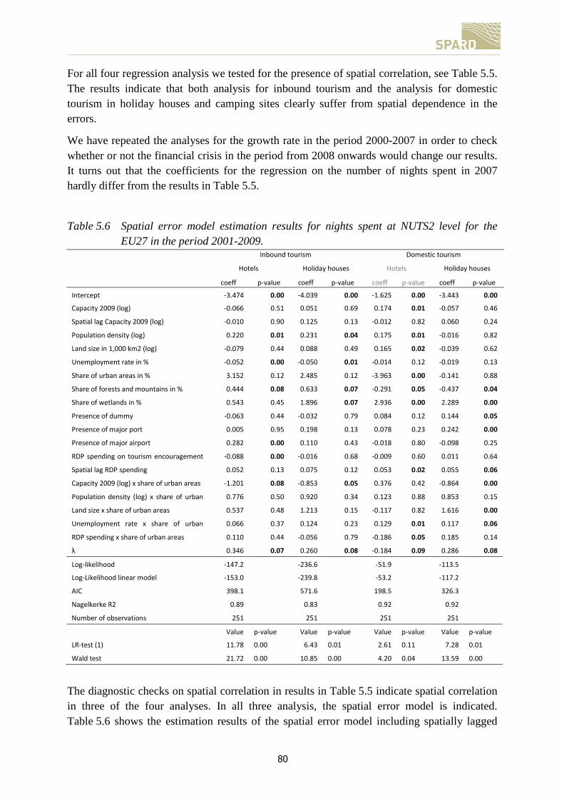
80

For all four regression analysis we tested for the presence of spatial correlation, see Table 5.5. The results indicate that both analysis for inbound tourism and the analysis for domestic tourism in holiday houses and camping sites clearly suffer from spatial dependence in the errors.

We have repeated the analyses for the growth rate in the period 2000-2007 in order to check whether or not the financial crisis in the period from 2008 onwards would change our results. It turns out that the coefficients for the regression on the number of nights spent in 2007 hardly differ from the results in Table 5.5.

Table 5.6 Spatial error model estimation results for nights spent at NUTS2 level for the EU27 in the period 2001-2009.




Intercept -3.474 0.00 -4.039 0.00 -1.625 0.00 -3.443 0.00

Capacity 2009 (log) -0.066 0.51 0.051 0.69 0.174 0.01 -0.057 0.46

Spatial lag Capacity 2009 (log) -0.010 0.90 0.125 0.13 -0.012 0.82 0.060 0.24

Population density (log) 0.220 0.01 0.231 0.04 0.175 0.01 -0.016 0.82

Land size in 1,000 km2 (log) -0.079 0.44 0.088 0.49 0.165 0.02 -0.039 0.62

Unemployment rate in % -0.052 0.00 -0.050 0.01 -0.014 0.12 -0.019 0.13

Share of urban areas in % 3.152 0.12 2.485 0.12 -3.963 0.00 -0.141 0.88

Share of forests and mountains in % 0.444 0.08 0.633 0.07 -0.291 0.05 -0.437 0.04

Share of wetlands in % 0.543 0.45 1.896 0.07 2.936 0.00 2.289 0.00

Presence of dummy -0.063 0.44 -0.032 0.79 0.084 0.12 0.144 0.05

Presence of major port 0.005 0.95 0.198 0.13 0.078 0.23 0.242 0.00

Presence of major airport 0.282 0.00 0.110 0.43 -0.018 0.80 -0.098 0.25

RDP spending on tourism encouragement -0.088 0.00 -0.016 0.68 -0.009 0.60 0.011 0.64

Spatial lag RDP spending 0.052 0.13 0.075 0.12 0.053 0.02 0.055 0.06

Capacity 2009 (log) x share of urban areas -1.201 0.08 -0.853 0.05 0.376 0.42 -0.864 0.00

Population density (log) x share of urban 0.776 0.50 0.920 0.34 0.123 0.88 0.853 0.15

Land size x share of urban areas 0.537 0.48 1.213 0.15 -0.117 0.82 1.616 0.00

Unemployment rate x share of urban 0.066 0.37 0.124 0.23 0.129 0.01 0.117 0.06

RDP spending x share of urban areas 0.110 0.44 -0.056 0.79 -0.186 0.05 0.185 0.14

λ 0.346 0.07 0.260 0.08 -0.184 0.09 0.286 0.08

Log-likelihood -147.2 -236.6 -51.9 -113.5

Log-Likelihood linear model -153.0 -239.8 -53.2 -117.2

AIC 398.1 571.6 198.5 326.3

Nagelkerke R2 0.89 0.83 0.92 0.92


Value p-value Value p-value Value p-value Value p-value

LR-test (1) 11.78 0.00 6.43 0.01 2.61 0.11 7.28 0.01

Wald test 21.72 0.00 10.85 0.00 4.20 0.04 13.59 0.00

The diagnostic checks on spatial correlation in results in Table 5.5 indicate spatial correlation in three of the four analyses. In all three analysis, the spatial error model is indicated. Table 5.6 shows the estimation results of the spatial error model including spatially lagged

81

variables for capacity and RDP spending. In comparison with the results in Table 5.5 the signs and magnitude of the coefficients do not change much due to the spatial error structure. All analysis are significant according to the Likelihood ratio test. The λ-parameter of the spatial error model is positive and significant in all models, which means that the results improve significantly when we take into account the spatial dependencies in the error terms.

In addition, we also included two spatially lagged variables in the spatial error models. The capacity of neighbouring regions did not have impact on any type of tourism in the region. For the RDP spending in neighbouring regions, however, we do find positive significant coefficients for domestic tourism. So, there are spillover effects from RDP spending from other regions on the tourism from inhabitants of a region. This indicates that there might be a demonstration effect spillovers present. Apparently, the tourism industry in a region learns from the developments in its neighbouring regions.

Spatial dependence The results for the static specification of the tourism model show that spatial dependence plays a role in the explanation of tourism in a number of ways. First of all, the explanatory spatial data analysis already showed the presence of spatial dependence in the tourism indicators and the spending on encouraging tourism. Secondly, by distinguishing between inbound and domestic tourism indicators we already take into account spatial dependence because both type of indicators have different types of spillovers. Thirdly, the spatial dependence tests for the linear model of the static specification indicate the presence of spatial errors in all cases. Finally, the spatial error model result are significant, and the spatially lagged variables for RDP spending are significant for the domestic tourism.

5.4.3 Dynamic specification

So far, we have focused on the spatial patterns in the explanation of tourism in a region. In the literature, however, there are also studies on tourism that focus on the temporal patterns of tourism. In this section, we extend the linear cross section specifications from Section 5.4.2 with a temporal dimension in order to check whether the temporal patterns are present and how those temporal patterns affect the results from the spatial patterns. We have got two alternatives. Firstly, we simply add the lagged number of number of nights spent in the specification. Secondly, we apply the convergence specification from the economic growth theory literature, in which we explain the changes in the number of nights spent in a specific period by the number of nights spent at the beginning of the period and other explanatory variables. For consistency with Chapter 3 and 4, we explore the first alternative and ignore the convergence models, since we are using logarithms for many variables, and the differences might be negative. Alternatively, we attempted to estimate growth factor models as is done in Chapter 4 but for tourism the result of those regression models showed limited explanatory power.

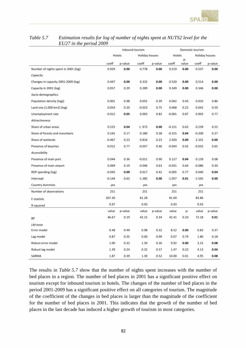
82

Table 5.7 Estimation results for log of number of nights spent at NUTS2 level for the

EU27 in the period 2009



coeff p-value coeff p-value coeff

p-

value coeff p-value

Number of nights spent in 2001 (log) 0.929 0.00 0.778 0.00 0.519 0.00 0.537 0.00

Capacity

Changes in capacity 2001-2009 (log) 0.447 0.00 0.332 0.00 0.520 0.00 0.514 0.00

Capacity in 2001 (log) 0.057 0.29 0.289 0.00 0.349 0.00 0.346 0.00

Socio-demographics

Population density (log)) 0.001 0.98 0.055 0.39 0.042 0.43 0.010 0.86

Land size (1,000 km2) (log) 0.054 0.20 -0.023 0.75 0.068 0.22 0.042 0.50

Unemployment rate -0.012 0.05 0.003 0.82 -0.001 0.87 0.003 0.77

Attractiveness

Share of urban areas 0.525 0.04 1. 973 0.00 -0.151 0.63 0.239 0.55

Share of forests and mountains 0.165 0.17 0.180 0.38 -0.315 0.04 -0.200 0.27

Share of wetlands -0.467 0.23 0.816 0.23 2.920 0.00 2.101 0.00

Presence of beaches -0.012 0.77 -0.057 0.46 -0.043 0.42 -0.032 0.65

Accessibility

Presence of main port 0.044 0.36 -0.011 0.90 0.127 0.04 0.139 0.08

Presence of main airport 0.069 0.19 -0.046 0.63 -0.031 0.64 -0.086 0.30

RDP spending (log) -0.045 0.00 0.017 0.42 -0.005 0.77 0.040 0.04

Intercept -0.144 0.62 -1.385 0.00 -1.057 0.01 -1.565 0.00

Country dummies yes

yes

yes

yes


F-statistic 207.30 81.28 81.69 83.86

R-squared 0.97 0.93 0.93 0.93

value p-value value p-value value p- value p-value

BP 46.67 0.19 42.15 0.34 42.41 0.10 72.18 0.01

LM-tests

Error model 0.48 0.49 0.98 0.32 8.52 0.00 0.83 0.37

Lag model 0.87 0.35 0.00 0.99 0.07 0.79 1.80 0.18

Robust error model 1.00 0.32 1.30 0.26 9.92 0.00 3.15 0.08

Robust lag model 1.39 0.24 0.32 0.57 1.47 0.23 4.13 0.04

SARMA 1.87 0.39 1.30 0.52 10.00 0.01 4.95 0.08

The results in Table 5.7 show that the number of nights spent increases with the number of bed places in a region. The number of bed places in 2001 has a significant positive effect on tourism except for inbound tourism in hotels. The changes of the number of bed places in the period 2001-2009 has a significant positive effect on all categories of tourism. The magnitude of the coefficient of the changes in bed places is larger than the magnitude of the coefficient for the number of bed places in 2001. This indicates that the growth of the number of bed places in the last decade has induced a higher growth of tourism in most categories.

83

As in the static specification, the impacts for population density and size of the area rate have no significant effect in the dynamic specification. The impact of the unemployment rate is insignificant, although it was significant in the static specification.

The share of urban areas has a significant positive impact on inbound tourism. A larger share of urban areas increases the domestic tourism, while a larger share of wetland increases domestic tourism. Also, the presence of a main port increases domestic tourism, while the presence of a main port does not affect inbound tourism which is in contrast to the results of the static specification. The RDP spending on the encouragement of tourism has a positive impact on domestic tourism in holiday houses (rural tourism) while it has a negative effect on the inbound tourism in hotels. The level of tourism in 2001 has a significant positive impact on the level of tourism in 2009. The coefficients for the level of tourism in 2001 are higher for inbound tourism than for domestic tourism. Spatial dependence

The diagnostic tests in the dynamic specification do not indicate spatial dependence for the inbound tourism indicators. This means that there are no spillover effects from other regions. Based on the comparison of the results of the static and dynamic specifications, the temporal effect of inbound tourism seems to eliminate the spatial dependence with other regions. The dynamic specification does not indicate demonstration effect, competition effect or market access spillovers. For domestic tourism in hotels, the LM test suggest the spatial error model. This means that demonstration effect spillovers might be present in domestic tourism. In order to test for the presence of this type of spillover effects, we explore a spatial error model for the dynamic specification of domestic tourism. For inbound tourism, we re-explore the linear model with additional spatially lagged variables for capacity and RDP spending.

Table 5.8 presents the results of the dynamic specification of the number of nights spent including spatially lagged variables. For the domestic tourism, we explored the spatial error model. The significance and values of the coefficient do not change much when we compare the results in Table 5.8 with the results in Table 5.7. For inbound tourism, the lack of spatial dependence is confirmed by the insignificant coefficients for the spatially lagged RDP spending and capacity in 2009. There is no evidence for spillover effects for the dynamic specification inbound tourism.

In the case of domestic tourism, the spatial error model improves the results. Firstly, there is evidence for spillover effects for RDP spending from neighbouring regions. This results confirms the results found for the static specification of domestic tourism. Secondly, the λ-parameter in the spatial error model is significantly negative for domestic tourism, which is rather unusual for spatial error models. However, the negative λ-parameter means that regions with high levels of domestic tourism in hotels for instance are likely to be adjacent to regions with low levels of domestic tourism in hotels. For domestic tourism in holiday houses the same applies. It might indicate that there are still unobserved explanatory variables which are not included in our model.

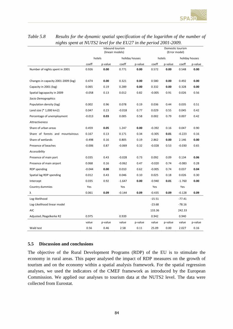
84

Table 5.8 Results for the dynamic spatial specification of the logarithm of the number of

nights spent at NUTS2 level for the EU27 in the period 2001-2009.

Inbound tourism

(lineair models)

Domestic tourism

(Error model)

hotels holiday houses hotels holiday houses


Number of nights spent in 2001 0.926 0.00 0.771 0.00 0.572 0.00 0.548 0.00

Changes in capacity 2001-2009 (log) 0.474 0.00 0.321 0.00 0.580 0.00 0.492 0.00

Capacity in 2001 (log) 0.065 0.19 0.289 0.00 0.332 0.00 0.328 0.00

Spatial lagcapacity in 2009 -0.058 0.13 0.012 0.82 -0.005 0.91 0.026 0.56

Socio Demographics

Population density (log) 0.002 0.96 0.078 0.19 0.036 0.44 0.035 0.51

Land size (* 1,000 km2) 0.047 0.23 -0.018 0.77 0.029 0.55 0.045 0.42

Percentage of unemployment -0.013 0.03 0.005 0.58 0.002 0.79 0.007 0.42

Attractiveness

Share of urban areas 0.459 0.05 1.247 0.00 -0.392 0.16 0.047 0.90

Share of forests and mountainous 0.167 0.13 0.171 0.34 -0.305 0.01 -0.223 0.16

Share of wetlands -0.498 0.16 0.805 0.19 2.862 0.00 2.146 0.00

Presence of beaches -0.006 0.87 -0.069 0.32 -0.028 0.53 -0.030 0.65

Accessibility

Presence of main port 0.035 0.43 -0.028 0.73 0.092 0.09 0.134 0.06

Presence of main airport 0.068 0.16 -0.062 0.47 -0.020 0.74 -0.083 0.28

RDP spending -0.044 0.00 0.010 0.62 -0.005 0.74 0.037 0.04

Spatial lag RDP spending 0.012 0.43 0.046 0.10 0.025 0.18 0.026 0.30

Intercept 0.035 0.92 -1.647 0.00 -0.940 0.01 -1.760 0.00

Country dummies Yes Yes Yes Yes

λ 0.061 0.09 -0.144 0.09 -0.435 0.09 -0.128 0.09

Log-likelihood -15.51 -77.41

Log-Likelihood linear model -23.68 -78.16

AIC 133.36 242.33

Adjusted /Nagelkerke R2 0.975 0.939 0.942 0.940

value p-value value p-value value p-value value p-value

Wald test 0.56 0.46 2.58 0.11 25.09 0.00 2.027 0.16


The objective of the Rural Development Programs (RDP) of the EU is to stimulate the economy in rural areas. This paper analysed the impact of RDP measures on the growth of tourism and on the economy within a spatial analysis framework. For the spatial regression analyses, we used the indicators of the CMEF framework as introduced by the European Commission. We applied our analyses to tourism data at the NUTS2 level. The data were collected from Eurostat.

85

The explanatory spatial data analysis clearly showed the spatial dependency of the tourism indicators, i.e. number of nights spent by non-residents. For three different years, the number of nights spent by non-residents were significantly different from zero. The spending on the RDP measure showed spatial dependence as well although the spending was not uniformly distributed over the years. As a result, we explored a regression analysis and tested for spatial dependencies afterwards. In the case of the tourism growth model, there is little evidence for spatial dependencies in the residuals of the model despite a significant positive Moran’s I. In the case of the absolute developments of tourism, spatial dependencies turned out to be present. The appropriate model was the spatial error model in a number of specifications of both the steady state and growth model. The capacity of tourism accommodations had a significant impact on tourism regardless the type of specification or model. In the ‘dynamic’ model, the growth of capacity induced additional growth of tourism. The presence of natural areas also had a positive impact. In both models we took into account spatial heterogeneity. We included country dummy variables, and we included spatial variables, such as share of land use and accessibility through ports and airport, which were incidentally significant for the tourism indicators.

The direct spending on the encouragement of tourism turned out to be insignificant, although the spatially lagged spending has a small positive impact. One reason for this finding might be the concentration of spending in particular part of the EU. Secondly, the spending is rather small compared to the economic value of the tourism sector. Moreover, the spending is often project-based. It is more likely that the impact of spending can be observed at lower levels, such as the level of municipalities for instance. Preferably, the spatial analysis is repeated at municipality level.

For analysing tourism, the spatial econometric approach is very suitable, because tourism data exhibits spatial dependence by nature. This is not necessarily shown by complicated spatial models but by straightforward linear or error models including spatially lagged variables explicitly. Based on our hypotheses, we would have expected significant evidence for spillovers in inbound tourism and modest impacts in domestic tourism. However, the results of our analysis indicate that modest spillovers are present in domestic tourism, and spillovers results in the static specification for inbound tourism turn out to be part of the temporal effect in inbound tourism.

86

6 Conclusions

6.1 Introduction

The SPARD project aims at developing tools to analyse to what extent EU rural development measures have the intended impact, either an impact on the economy, such as through labour productivity growth, economic growth and tourism, or a contribution to the realization of environmental targets. The analyses is based upon CMEF, the EU common monitoring and evaluation framework of RDP measures. For measures from the three Axes of the RDP, we constructed spatial models, based on economic theory, to show that this approach is feasible. We estimated these models spatial econometrically, using data from Eurostat and from Cambridge Econometrics (CE) at NUTS2 level to test whether we could find evidence for the intended effect of selected measures. The results clearly indicate that spatial analyses and spatial econometrics improve the assessment of RPD measures. The measures analysed all require measure-specific models with measure-specific data.

In this concluding Chapter we return to our main research questions. In particular, we elaborate on the answer of the question “did spatial analysis matter in the evaluation of the effectiveness of the RDP measures?” in Section 6.2. The answers result from the analysis in Chapters 3 to 5. Finally, we discuss a number of issues how the spatial analyses for RDP evaluation can be improved.

6.2 Did spatial analysis matter?

The results of the assessments in Chapters 3 to 5 clearly indicate that it is important to take into account spatial dependence in the assessment of RDP measures. Table 6.1 summarizes the spatial dependence in the data and econometric estimations for the different assessments.

In the case of agricultural labour productivity, agri-environmental measures and tourism analysis, we found that spatial dependency is present in the dependent variables (the result indicator). Especially, agricultural labour productivity and nitrogen surplus showed high Moran’s I statistics. In the case of tourism, the Moran’s I statistics were modest but significantly different from 0.

87

Table 6.1 Spatial error model estimation results for nights spent at NUTS2 level for the EU27 in the period 2001-2009.

Labour

productivity in

agriculture

Environmental models Tourism

N-surplus HNV indicator

Level of analyses NUTS2 NUTS0 NUTS 1 and

combined

NUTS2

Data source CE CE/EUROSTAT CE/EUROSTAT EUROSTAT

Type of data Cross section Panel data Cross section Cross section

Spatial dependence in data

-Indicators Yes Yes Yes Yes

-Spending

Weight matrix Gabriel Gabriel Gabriel Queen contiguity

Spatial dependence in

regressions

Type of spatial model Spatial error

model

Spatial panel Spatial lag

model

Spatial error model

Spending

Spatially lagged spending Yes Yes Yes

Cross spending effects tested Yes Yes Yes No

Spatial heterogeneity

-Country specific dummies Yes No Yes

-Regime dummies/coefficients Yes Yes (steady state)

-Regional specific variables Yes Yes Yes

In all analyses of the RDP axes 1 (agricultural labour productivity), 2 (nitrogen surplus) and 3 (tourism), there is only little evidence for the effects of spending of particular measures on either impact or result indicators. For the HNV-index we could not detect this relation. There are different reasons to explain these results.

Firstly, at NUTS2 level, the correlation of spending and three dependent variables (agricultural labour productivity, HNV-index, tourism) is apparently negligible or weak. The spending on RDP measures is small compared to the GVA and investments,. This especially applies to measure 311 and 313. Secondly, as we have described in the previous chapters, the impact of RDP measures is for measure 121, measure 214 and measure 311 best measured at the farm level (measure 313 is not focussed on farms). The impact at a lower aggregation level will be difficult to prove at the aggregated NUTS2 level.

Our analyses heavily rely on the presence of good quality data sets. Without data, we cannot explore the spatial data analysis or the spatial econometric analysis. We selected the relevant characteristics or explanatory not only from the CMEF framework but also from the economic literature. At NUTS 2 level, we collected data from the EU (on spending), Eurostat and Cambridge Econometrics. For many NUTS2 regions, data, that reflect the impact or result

88

indicators, were present. For our HNV-index we constructed an index based on Farm Structure Survey at NUTS2 level and for nitrogen surplus we had to use data at NUTS0 level. For all results of impact indicators we used as dependent variables a time series of indicators, so that the change in the indicators could be analysed and related to the spending.

Due to the fact that we apply spatial analyses, particular NUTS2 regions, such as the islands and overseas areas, drop out of the analysis for practical reasons. According to our spatial models of the dependent variables, this hardly effects our analysis. In addition, a few other NUTS2 areas were excluded because particular variables relevant for the spatial econometric analyses were lacking. In the case of tourism data, we first tried to impute data for other years before excluding NUTS2 areas. Approximately 16% of the NUTS2 regions were ultimately excluded in the spatial econometric analysis with small differences in the three different analyses.

Next to the spatial dependence, our models also took into account spatial heterogeneity. In the agricultural labour productivity analyses, regime dummies were tested and interacted with the RDP expenditures. The impact of RDP expenditures on labour productivity is stronger in southern rural and urban regions, and also in northern intermediate regions of the EU. In the case of water quality, a panel analyses was explored with random effects and a particular impact for Eastern EU Member States was tested and found not to be significant.

For biodiversity, spatial variables, such as acreage and share of other farmland, were tested. These spatial variables were insignificant. Finally, the tourism model accounted for spatial heterogeneity by including country specific effects and spatial variables such as the accessibility and land use share. Land use variables such as share of wetland in the area and presences of ports and airports were significant for one or more tourism indicators. Note that we already distinguished between domestic and in-bound tourism indicators which already includes a choice of location by tourists.

6.3 How to continue?

The spatial econometric analyses in this report can still be improved in order to resolve remaining issues such as heterogeneity problems and missing relevant explanatory variables. So far, the econometric analyses focused on the spatial econometric specifications for the dependent variables (agricultural labour productivity, environmental indicator, and tourism).

With respect to the case study analyses, the three spatial analyses provide a useful guide to start exploring a similar analyses at lower aggregation levels. The first step is to make sure that result or impact indicators are available. Note that the indicators in the spatial analyses of the different Axes do not have to be exactly the same as the indicators used in this report. In the case of agriculture labour productivity, one can also use one of the alternative result/impact indicators suggested in the CMEF framework. In the case of tourism, one could use employment in the tourism sector instead of number of nights spent. In addition, relevant characteristics have to be selected from the literature and their data availability have to be checked. The spatial data analyses and spatial econometric analyses as presented in this report can be explored at the case study as well if sufficient and relevant data are available.

89

In addition, the question whether spatial econometrics contributes to the assessment of the Rural Development Programme is answered and discussed in another Work Package of the SPARD project, see Reinhard and Linderhof (2013).

90

Acknowledgement We are very grateful to Raymond Florax for his advice during the estimation processes and his valuable comments on earlier drafts of this report. All maps are © EuroGeographics for the administrative boundaries

91

References Abramovitz, M. (1986). 'Catching Up, Forging Ahead, and Falling Behind', Journal of

Economic History, vol. 46(2), pp. 385-406.

Abreu, M., H. L. F. de Groot and R. J. G. M. Florax (2005). 'A Meta-Analysis of Beta-Convergence: the Legendary 2%', Journal of Economic Surveys, vol. 19(3), pp. 389-420.

Agra, C. (2005) Synthesis of rural development mid-term evaluation, LOT 11 EAGGF Guidance. Final report for European Commission. Available at http://www.ceasc.com/Images/Content/2181%20final%20report.pdf.

Albrecht, M., P. Duelli, C. Muller, D. Kleijn and B. Schmid (2007). 'The Swiss agri-environment scheme enhances pollinator diversity and plant reproductive success in nearby intensively managed farmland', Journal of Applied Ecology, vol. 44(4), pp. 813-822.

Andersen, E., D. Baldock, H. Bennett, G. Beaufoy, E. Bignal, F. Brouwer, B. Elbersen, G. Eiden, F. Godeschalk, G. Jones, D. McCracken, W. Nieuwenhuizen, M. Van Eupen, S. Hennekens and G. Zervas (2003) Developing a High Nature Value Farming area indicator, Copenhagen, European Environment Agency.

Anselin, L. (2002). 'Under the Hood: Issues in the Specification and Interpretation of Spatial Regression Models', Agricultural Economics, vol. 27(3), pp. 247-267.

Anselin, L. (2006). 'How (Not) to Lie with Spatial Statistics', American Journal of Preventive Medicine, vol. 30(2S), pp. 3-6.

Anselin, L. (2010). 'Thirty years of spatial econometrics', Papers in Regional Science, vol. 89(1), pp. 3-25.

Anselin, L., A. K. Bera, R. J. G. M. Florax and M. J. Yoon (1996). 'Simple Diagnostic Tests for Spatial Dependence', Regional Science and Urban Economics, vol. 26(1), pp. 77-104.

Anselin, L. and R. J. G. M. Florax (1995). New Directions in Spatial Econometrics, Berlin: Springer.

Anselin, L., J. Le Gallo, H. Jayet, L. M ty s and P. Sevestre (2008). 'Spatial Panel Econometrics', in (Marquez, J., A. Spanos, F. G. Adams, P. Balestra, M. G. Dagenais, D. Kendrick, J. H. P. Paelinck, R. S. Pindyck and W. Welfe Eds.), The Econometrics of Panel Data, pp. 625-660, Berlin/Heidelberg: Springer.

Anselin, L., N. Lozano-Gracia, T. C. Mills and K. Patterson (2009). 'Spatial Hedonic Models', Palgrave handbook of econometrics, pp. 1213-1250, Houndmills: Palgrave Macmillan.

Antle, J. M. and S. M. Capalbo (2001). 'Econometric-process models for integrated assessment of agricultural production systems', American Journal of Agricultural Economics, vol. 83(2), pp. 389-401.

Ausden, M. and R. J. Fuller (2009). 'Birds and habitat change in Britain Part 2: past and future conservation responses', British Birds, vol. 102(2), pp. 52-71.

Azariadis, C. and A. Drazen (1990). 'Threshold Externalities in Economic Development', The Quarterly Journal of Economics, vol. 105(2), pp. 501-526.

Baer, S. G., D. M. Engle, J. M. H. Knops, K. A. Langeland, B. D. Maxwell, F. D. Menalled and A. J. Symstad (2009). 'Vulnerability of Rehabilitated Agricultural Production Systems to Invasion by Nontarget Plant Species', Environmental Management, vol. 43(2), pp. 189-196.

92

Bailey, S. (2007). 'Increasing connectivity in fragmented landscapes: An investigation of evidence for biodiversity gain in woodlands', Forest Ecology and Management, vol. 238(1-3), pp. 7-23.

Baltagi, B. H., S. H. Song, J. B. and W. Koh (2007). 'Testing panel data regression models with spatial and serial error correlation', Journal of Econometrics, vol. 140, pp. 5-51.

Baltagi, B. H., S. H. Song and W. Koh (2003). 'Testing panel data regression models with spatial error correlation', Journal of Econometrics, vol. 117, pp. 123-150.

Bardhan, P. K. (1973). 'Size, Productivity, and Returns to Scale: An Analysis of Farm-Level Data in Indian Agriculture', Journal of Political Economy, vol. 81(6), pp. 1370-1386.

Basile, R. (2009). 'Productivity Polarization across Regions in Europe The Role of Nonlinearities and Spatial Dependence', International Regional Science Review, vol. 32, pp. 92.

Beaufoy, G., D. Baldock and J. Clark (1994) The Nature of Farming: Low Intensity Farming Systems in Nine European Countries, London, Institute for European Environmental Policy.

Beck, M. and T. Dogot 'The use of impact indicators for the evaluation of farm investment support - a case study based on the rural development programme for Wallonia (2000-2006)', in (Bergschmidt, A., W. Dirksmeyer, J. Efken and B. Forstner Eds.), Proceedings of the European Workshop on the Evaluation of Farm Investment Support and Investment Support for Improvement of Processing and Marketing of Agricultural Products, pp. 69-77.

Bergschmidt, A., W. Dirksmeyer, J. Efken and B. Forstner (2006) Proceedings of the European Workshop on the Evaluation of Farm Investment Support and Investment Support for Improvement of Processing and Marketing of Agricultural Products

Bernini, C. and A. Guizzardi (2010). 'Internal and locational factors affecting hotel industry efficiency: evidence from Italian business corporations', Tourism Economics, vol. 16(4), pp. 883-913.

Beugelsdijk, S. (2007). 'The Regional Environment and a Firm's Innovative Performance: A Plea for a Multilevel Interactionist Approach', Economic Geography, vol. 83(2), pp. 181-199.

Billeter., R., J. Liira, D. Bailey, R. Bugter, P. Arens, I. Augenstein, S. Aviron, J. Baudry, R. Bukacek, F. Burel, M. Cerny, G. De Blust, R. De Cock, T. Diekötter, H. Dietz, J. Dirksen, C. Dormann, W. Durka, M. Frenzel, R. Hamersky, F. Hendrickx, F. Herzog, S. Klotz, B. Koolstra, A. Lausch, D. Le Coeur, J. P. Maelfait, P. Opdam, M. Roubalova, A. Schermann, N. Schermann, T. Schmidt, O. Schweiger, M. J. M. Smulders, M. Speelmans, P. Simova, J. Verboom, W. K. R. E. Van Wingerden, M. Zobel and P. J. Edwards (2008). 'Indicators for biodiversity in agricultural landscapes: a pan-European study', Journal of Applied Ecology, vol. 45, pp. 141-150.

Boschma, R. A. (2005). 'Role of Proximity in Interaction and Performance: Conceptual and Empirical Challenges (editorial)', Regional Studies, vol. 39(1), pp. 41-45.

Brau, R., A. Lanza and P. F. (2004). 'How fast are tourism countries growing? The cross country evidence', in (Lanza, A., A. Markandya and F. Pigliaru Eds.), The Economics of Tourism and Sustainable Development, Cheltenham, UK: Edward Elgar.

Brau, R., A. Lanza and F. Pigliaru (2007). 'How fast are small tourism countries growing? Evidence from the data for 1980-2003', Tourism Economics, vol. 13, pp. 603-613.

Brereton, T. M., M. S. Warren, D. B. Roy and K. Stewart (2008). 'The changing status of the Chalkhill Blue butterfly Polyommatus coridon in the UK: the impacts of conservation

93

policies and environmental factors', Journal of Insect Conservation, vol. 12(6), pp. 629-638.

Bro, E., P. Mayot, E. Corda and F. Reitz (2004). 'Impact of habitat management on grey partridge populations: assessing wildlife cover using a multisite BACI experiment', Journal of Applied Ecology, vol. 41(5), pp. 846-857.

Bullock, J. M., R. F. Pywell and K. J. Walker (2007). 'Long-term enhancement of agricultural production by restoration of biodiversity', Journal of Applied Ecology, vol. 44(1), pp. 6-12.

Bussler, H., D. Dujesiefken and P. Kockenbeck (2006). 'Der Zielkonflikt zwischen Artenschutz und Verkehrssicherheit - xylobionte K„ferarten der FFH-Richtlinie in Bayern', Jahrbuch der Baumpflege 2006 (Yearbook of Arboriculture). pp. 113-118, Braunschweig, 288 p.

Carey, P. D., S. J. Manchester and L. G. Firbank (2005). 'Performance of two agri-environment schemes in England: a comparison of ecological and multi-disciplinary evaluations', Agriculture Ecosystems & Environment, vol. 108(3), pp. 178-188.

Coase, R. H. and R. F. Fowler (1935). 'Bacon Production and the Pig-Cycle in Great Britain', Economica, vol. 2(6), pp. 142-167.

Collado Cueto, L. A. (2006). 'Effectiveness and impacts of farm investment support in Spain - the experience of the updated mid-term evaluation (2000-2006)', in (Bergschmidt, A., W. Dirksmeyer, J. Efken and B. Forstner Eds.), Proceedings of the European Workshop on the Evaluation of Farm Investment Support and Investment Support for Improvement of Processing and Marketing of Agricultural Products, pp. 105-120.

Com (2005) Agri-environment Measures - Overview on General Principles, Types of Measures, and Application, European Commission, Directorate General for Agriculture and Rural Development, Unit G-4 - Evaluation of Measures applied to Agriculture, Studies. Available at http://ec.europa.eu/agriculture/publi/reports/agrienv/rep_en.pdf.

Com (2006a) Common Monitoring and Evaluation Framework. Guidance document, Directorate General for Agriculture and Rural Development. Available at http://ec.europa.eu/agriculture/rurdev/eval/guidance/document_en.pdf.

COM (2006b) The EU rural development policy 2007-2013.

Critchley, C. N. R., M. J. W. Burke and D. P. Stevens (2004). 'Conservation of lowland semi-natural grasslands in the UK: a review of botanical monitoring results from agri-environment schemes', Biological Conservation, vol. 115(2), pp. 263-278.

Da-Rocha, J. M. and D. Restuccia (2006). 'The role of agriculture in aggregate business cycles', Review of Economic Dynamics, vol. 9(3), pp. 455-482.

de Wit, M., M. Londo and A. Faaij (2011). 'Productivity developments in European agriculture: Relations to and opportunities for biomass production', Renewable and Sustainable Energy Reviews, vol. 15(5), pp. 2397-2412.

Deumlich, D., J. Kiesel, J. Thiere, H. I. Reuter, L. Volker and R. Funk (2006). 'Application of the SIte COmparison Method (SICOM) to assess the potential erosion risk - a basis for the evaluation of spatial equivalence of agri-environmental measures', Catena, vol. 68(2-3), pp. 141-152.

Diewert, W. E. (1971). 'An application of the Shephard Duality Theorem: A General Leontief Production Function', Journal of Political Economy, vol. 79(3), pp. 481-507.

Diewert, W. E. (1974). 'Functional forms for revenue and factor requirement functions', International Economic Review, vol. 15, pp. 119-130.

Dol, W. and D. Godeschalk (2011). 'MetaBase, The Hague: LEI Wageningen UR.

94

Donald, P. F. and J. A. Vickery (2000). 'The importance of cereal fields to breeding and wintering Skylarks Alauda arvensis in the UK', Ecology and Conservation of Lowland Farmland Birds, pp. 140-150.

Dosi, G. (1982). 'Technological paradigms and technological trajectories: a suggested interpretation of the determinants and directions of technical change', Research Policy, vol. 11(3), pp. 147-162.

Duelli, P. and M. K. Obrist (2003). 'Regional biodiversity in an agricultural landscape: The contribution of seminatural habitat islands', Basic and Applied Ecology, vol. 4, pp. 129-138.

Dwyer, J., J. Kirwan, K. Thomson, M. Clark, C. Kambites, N. Lewis and A. Molnarova (2008) Review of Rural Development Instruments. DG Agri project 2006-G4-10. Final Report (With colleagues at INEA, IfLS, IEEP, VUZE, AgraCeas Consulting Ltd). Available at http://ec.europa.eu/agriculture/analysis/external/rurdev/full_report_en.pdf.

Dwyer, L., P. Forsyth and R. Spurr (2004). 'Evaluating tourism’s economic effects: new and old approaches', Tourism Management, vol. 25, pp. 307-317.

EC (2006) The Guidance Note E – measure fiches of the guidance document of the CMEF for the Rural Development 2007-2013, Brussels. Available at http://ec.europa.eu/agriculture/rurdev/eval/index_en.htm.

EC (2009) Guidance document; The application of the High Nature Value Impact Indicator; Programming Period 2007-2013, Brussels. Available at http://ec.europa.eu/agriculture/rurdev/eval/hnv/guidance_en.pdf.

Ederveen, S., H. L. de Groot and R. Nahuis (2006). 'Fertile Soil for Structural Funds? A Panel Data Analysis of the Conditional Effectiveness of European Cohesion Policy', Kyklos, vol. 59(1), pp. 17-42.

Ederveen, S., J. Gorter, R. de Mooij and R. Nahuis (2002) Funds and Games; The Economics of European Cohesion Policy, The Hague, CPB Netherland’s Bureau for Economic Policy Analysis.

Edwards, A. R., S. R. Mortimer, C. S. Lawson, D. B. Westbury, S. J. Harris, B. A. Woodcock and V. K. Brown (2007). 'Hay strewing, brush harvesting of seed and soil disturbance as tools for the enhancement of botanical diversity in grasslands', Biological Conservation, vol. 134(3), pp. 372-382.

EEA (2004) High Nature Value Farmland: Characteristics, Trends and Policy Challenges, Copenhagen, European Environment Agency.

Elhorst, J. P. (2003). 'Specification and estimation of spatial panel data models', International Regional Science Review, vol. 26(3), pp. 244.

Ertur, C., J. Le Gallo and C. Baumont (2006). 'The European Regional Convergence Process, 1980-1995: Do Spatial Regimes and Spatial Dependence Matter?', International Regional Science Review, vol. 29(1), pp. 3-34.

Ezcurra, R., B. Iraizoz, P. Pascual and M. Rapun (2010). 'Agricultural Productivity in the European Regions: Trends and Explanatory Factors', European Urban and Regional Studies, vol. 18(2), pp. 113-135.

Figini, P. and L. Vici (2010). 'Tourism and growth in a cross section of countries', Tourism Economics, vol. 16(4), pp. 789-805.

Fingleton, B. (2008). 'A generalized method of moments estimator for a spatial panel model with an endogenous spatial lag and spatial moving average errors', Spatial Economic Analysis, vol. 3(1), pp. 27-44.

95

Florax, R. J. G. M. and A. J. Van der Vlist (2003). 'Spatial Econometric Data Analysis: Moving Beyond Traditional Models', International Regional Science Review, vol. 26(3), pp. 223.

Florax, R. J. G. M., R. L. Voortman and J. Brouwer (2002). 'Spatial dimensions of precision agriculture: a spatial econometric analysis of millet yield on Sahelian coversands', Agricultural Economics, vol. 27(3), pp. 425-443.

Forstner, B., A. Bergschmidt, W. Dirksmeyer, H. Ebers, A. Fitschen-Lischewski, A. Margarian and J. Heuer (2009) Ex-Post-Bewertung des Agrarinvestitionsförderungsprogramms (AFP) im Förderzeitraum 2000 bis 2006, Johann Heinrich von Thünen-Institut.

Fulginiti, L. and R. Perrin (1998). 'Agricultural Productivity in Developing Countries', Agricultural Economics, vol. 19(1-2), pp. 45-51.

Gabriel, K. R. and R. R. Sokal (1969). 'A New Statistical Approach to Geographic Variation Analysis', Systematic Biology, vol. 18(3), pp. 259-278.

Gallo Le, J. and S. Dall'erba (2008). 'Spatial and sectoral productivity convergence between European regions, 1975-2000', Papers in Regional Science, vol. 87(4), pp. 505-525.

Geoghegan, J., L. Lynch and S. Bucholtz (2003). 'Capitalization of open spaces into housing values and the residential property tax revenue impacts of agricultural easement programs', Agricultural and Resource Economics Review, vol. 32(1), pp. 33-45.

Gershon, F. (1985). 'The relation between farm size and farm productivity: The role of family labor, supervision and credit constraints', Journal of Development Economics, vol. 18(2-3), pp. 297-313.

Getis, A. (2009). 'Spatial Weights Matrices', Geographical Analysis, vol. 41, pp. 404-410.

Goel, R. K. and J. Budak (2010). 'Tourism policies and cross-country growth: a disaggregated analysis', Tourism Economics, vol. 16(3), pp. 535-548.

Gollin, D., P. Pingali and R. Evenson (2010). 'Agricultural Productivity and Economic Growth', Handbook of Agricultural Economics, pp. 3825-3866, Oxford/Amsterdam: Elsevier.

Granlund, K., A. Raike, P. Ekholm, K. Rankinen and S. Rekolainen (2005). 'Assessment of water protection targets for agricultural nutrient loading in Finland', Journal of Hydrology, vol. 304(1-4), pp. 251-260.

Grovermann, C., P. Schreinemachers and T. Berger (2012). 'Private and social levels of pesticide overuse in rapidly intensifying upland agriculture in Thailand, City.

Hall, R. E. and C. I. Jones (1999). 'Why Do Some Countries Produce So Much More Output per Worker than Others?', Quarterly Journal of Economics, vol. 114(1), pp. 83-116.

Hanley, N., M. Whitby and I. Simpson (1999). 'Assessing the success of agri-environmental policy in the UK', Land Use Policy, vol. 16(2), pp. 67-80.

Hayami, Y. and V. W. Ruttan (1970). 'Agricultural Productivity Differences among Countries', American Economic Review, vol. 60(5), pp. 895-911.

Herzog, F., S. Dreier, G. Hofer, C. Marfurt, B. Schüpbach, M. Spiess and T. Walter (2005). 'Effect of ecological compensation areas on floristic and breeding bird diversity in Swiss agricultural landscapes', Agriculture, Ecosystems & Environment, vol. 108(3), pp. 189-204.

Herzog, F., B. Steiner, D. Bailey, J. Baudry, R. Billeter, R. Bukacek, G. De Blust, R. De Cocke, J. Dirksen, C. F. Dormanng, R. De Filippi, E. Frossard, J. Liira, T. Schmidt, R. Stockli, C. Thenail, W. Van Wingerden and R. Bugter (2006). 'Assessing the intensity

96

of temperate European agriculture at the landscape scale', European Journal of Agronomy, vol. 24, pp. 165-181.

Hodge, I. (2000). 'Agri-environmental Pelationships and the Choice of Policy Mechanism', The World Economy, vol. 23(2), pp. 257-273.

Hodge, I. and S. McNally (1998). 'Evaluating the environmentally sensitive areas: the value of rural environments and policy relevance', Journal of Rural Studies, vol. 14(3), pp. 357-367.

Hodge, I. and S. McNally (2000). 'Wetland restoration, collective action and the role of water management institutions', Ecological Economics, vol. 35(1), pp. 107-118.

Hodge, I. and M. Reader (2009). 'The introduction of Entry Level Stewardship in England: Extension or dilution in agri-environment policy?', Land Use Policy, vol. 27, pp 744-754.

Hopkins, A., R. F. Pywell, S. Peel, R. H. Johnson and P. J. Bowling (1999). 'Enhancement of botanical diversity of permanent grassland and impact on hay production in Environmentally Sensitive Areas in the UK', Grass and Forage Science, vol. 54(2), pp. 163-173.

Huffman, W. E., B. L. Gardner and G. C. Rausser (2001). 'Human capital: Education and agriculture', Handbook of Agricultural Economics, pp. 333-381, Oxford/Amsterdam: Elsevier.

Hussler, C. (2004). 'Culture and knowledge spillovers in Europe: New perspectives for innovation and convergence policies?', Economics of Innovation and New Technology, vol. 13(6), pp. 523-541.

Kelejian, H. and I. R. Prucha (2001). 'On the asymptotic distribution of the Moran I test statistic with applications', Journal of Econometrics, vol. 104(2), pp. 219-257.

Kleijn, D. (2006). 'Ecological effects of agri-environment schemes on birds in different European countries', Journal of Ornithology, vol. 147, pp. 20-21.

Kleijn, D., R. A. Baquero, Y. Clough, M. Diaz, J. De Esteban, F. Fernandez, D. Gabriel, F. Herzog, A. Holzschuh, R. Johl, E. Knop, A. Kruess, E. J. P. Marshall, I. Steffan-Dewenter, T. Tscharntke, J. Verhulst, T. M. West and J. L. Yela (2006). 'Mixed biodiversity benefits of agri-environment schemes in five European countries', Ecology Letters, vol. 9(3), pp. 243-254.

Kleijn, D., F. Berendse, R. Smit and N. Gilissen (2001). 'Agri-environment schemes do not effectively protect biodiversity in Dutch agricultural landscapes', Nature, vol. 413(6857), pp. 723-725.

Krugman, P. (1996). Pop Internationalism, Cambridge (MA): MIT Press. Kumbhakar, S. C. (1994). 'A multiproduct symmetric generalized McFadden cost function',

Journal of Productivity Analysis, vol. 5, pp. 349-357.

LeSage, J. P. (1999). The Theory and Practice of Spatial Econometrics, Toledo: University of Toledo.

LeSage, J. P. and R. K. Pace (2010). The Biggest Myth in Spatial Econometrics, Toledo: University of Toledo.

.

Linderhof, V., P. Nowicki, E. van Leeuwen, S. Reinhard and M. J. Smit (2011) Manual for Testing a Spatial Econometric Model, D4.1.

Longhi, S. and P. Nijkamp (2007). 'Forecasting regional labor market developments under spatial autocorrelation', International Regional Science Review, vol. 30(2), pp. 100-119.

97

Lukesch, R. and B. Schuh (2010) Approaches for assessing the impacts of the Rural Development Programmes in the context of multiple intervening factors, European Commission - Agriculture and Rural Development, Findings of a Thematic Working Group established and coordinated by the European Evaluation Network for Rural Development. Available at http://ec.europa.eu/agriculture/rurdev/eval/network/impacts_interactive_en.pdf.

Mankiw, N. G., D. Romer and D. N. Weil (1992). 'A Contribution to the Empirics of Economic Growth', Quarterly Journal of Economics, pp. 407-437.

Marriott, C. A., G. R. Bolton, J. M. Fisher and K. Hood (2005). 'Short-term changes in soil nutrients and vegetation biomass and nutrient content following the introduction of extensive management in upland sown swards in Scotland, UK', Agriculture Ecosystems & Environment, vol. 106(4), pp. 331-344.

Marrocu, E. and R. Paci (2011). 'They arrive with new information. Tourism flows and production efficiency in the European regions', Tourism Management, vol. 32(4), pp. 750-758.

Masters, W. A. and M. S. McMillan (2001). 'Climate and Scale in Economic Growth', Journal of Economic Growth, vol. 6, pp. 167-186.

Matula, D. W. and R. R. Sokal (1980). 'Properties of Gabriel Graphs Relevant to Geographic Variation Research and the Clustering of Points in the Plane', Geographical Analysis, vol. 12(3), pp. 205-222.

Meyer, S. (2006). 'Methods for the evaluation of investment support', in (Bergschmidt, A., W. Dirksmeyer, J. Efken and B. Forstner Eds.), Proceedings of the European Workshop on the Evaluation of Farm Investment Support and Investment Support for Improvement of Processing and Marketing of Agricultural Products, pp. 3-14.

Millo, G. and G. Piras (2012). 'splm: Spatial Panel Data Models in R', Journal of Statistical Software, vol. 47(1), pp. 1-38.

Morley, C. L. (2009). 'Dynamics in the specification of tourism demand models', Tourism Economics, vol. 15(1), pp. 23-39.

Nelson, G. C. and D. Hellerstein (1997). 'Do roads cause deforestation? Using satellite images in econometric analysis of land use', American Journal of Agricultural Economics, pp. 80-88.

Neumann, K., P. H. Verburg, E. Stehfest and C. Müller (2010). 'The yield gap of global grain production: A spatial analysis.', Agricultural Systems, vol. 103(5), pp. 316-326.

Newman, D. and A. Paasi (1998). 'Fences and neighbours in the postmodern world: boundary narratives in political geography', Progress in Human Geography, vol. 22(2), pp. 186-207.

Niebuhr, A. (2002). 'Spatial dependence of regional unemployment in the European Union', Discussion Paper Series.

Nissan, E., M. A. Galindo and M. T. Mendez (2011). 'Relationship between tourism and economic growth', Service Industries Journal, vol. 31(10), pp. 1567-1572.

O'Donnell, C. J., C. R. Shumway and V. E. Ball (1999). 'Input Demands and Inefficiency in U.S. Agriculture', American Journal of Agricultural Economics, vol. 81(4), pp. 865-880.

Oecd (2001) Measuring Productivity: Measurement of Aggregate and Industry-Level Productivity Growth, Paris, OECD.

Pack, B. (2011) The Road Ahead for Scotland: Final Report of the Inquiry into Future Support for Agriculture in Scotland, Edinburgh, The Scottish Government. Available at http://www.scotland.gov.uk/Resource/Doc/329281/0106448.pdf.

98

Paelinck, J. H. P. (2005). Spatial Econometrics: History, State-of-the-art and Challenges Ahead, City: Institute for World Economics.

Paelinck, J. H. P. and L. H. Klaassen (1979). Spatial econometrics, Farnorough: Saxon House.

Paracchini, M. L. (2006) Indicator ENV6; Biodiversity, flora, fauna and landscapes/High Nature Value Farmland; State Indicator, Ispra.

Paracchini, M. L. and W. Britz (2010) Quantifying effects of changed farm practices on biodiversity in policy impact assessment – an application of CAPRI-Spat, Ispra, Institute for Environment and Sustainability of the Joint Research Centre, European Commission.

Paracchini, M. L., J.-E. Petersen, Y. Hoogeveen, C. Bamps, I. Burfield and V. S. C. (2008) High Nature Value Farmland in Europe; An Estimate of the Distribution Patterns on the Basis of Land Cover and Biodiversity Data, Luxembourg, Institute for Environment and Sustainability of the Joint Research Centre, European Commission.

Parrott, A. and H. Burningham (2008). 'Opportunities of, and constraints to, the use of intertidal agri-environment schemes for sustainable coastal defence: A case study of the Blackwater Estuary, southeast England', Ocean & Coastal Management, vol. 51(4), pp. 352-367.

Patton, M. and S. McErlean (2003). 'Spatial effects within the agricultural land market in Northern Ireland', Journal of Agricultural Economics, vol. 54(1), pp. 35-54.

Payne, J. E. and A. Mervar (2010). 'Research note: The tourism-growth nexus in Croatia', Tourism Economics, vol. 16(4), pp. 1089-1094.

Peerlings, J. and N. Polman (2008). 'Agri-environmental contracting of Dutch dairy farms: the role of manure policies and the occurrence of lock-in', European Review of Agricultural Economics, vol. 35(2), pp. 167-191.

Pykälä, J. (2007). Maintaining plant species richness by cattle grazing: mesic semi-natural grasslands as focal habitats, PhD thesis. University of Helsinki.

Reinhard, A. J. (1999). ' Econometric analysis of economic and environmental efficiency of Dutch dairy farms, pp. 174, Wageningen: Wageningen Agricultural University.

Reinhard, A. J. and V. Linderhof (2013) Using spatial econometrics in impact assessment, SPARD deliverable D4.5. The Hague, LEI-Wageningen UR.

Reinhard, A. J., C. A. K. Lovell and T. G. (1999). 'Econometric Estimation of Technical and Environmental Efficiency: An Application to Dutch Dairy Farms ', American Journal of Agricultural Economics, vol. 81(1), pp. 44-60.

Rey, S. J., J. Le Gallo, T. C. Mills and K. Patterson (2009). 'Spatial Analysis of Economic Convergence', Palgrave Handbook of Econometrics, pp. 1251-1292, Houndmills: Palgrave Macmillan.

Sengupta, S. and D. E. Osgood (2003). 'The value of remoteness: a hedonic estimation of ranchette prices', Ecological Economics, vol. 44(1), pp. 91-103.

Solow, R. M. (1956). 'A Contribution to the Theory of Economic Growth', Quarterly Journal of Economics, vol. 70(1), pp. 65-94.

Sutherland, W. J. (2004). 'A blueprint for the countryside', Ibis, vol. 146, pp. 230-238.

Swan, T. W. (1956). 'Economic Growth and Capital Accumulation', Economic Record, vol. 32(2), pp. 334-361.

Torre, A. and A. Rallet (2005). 'Proximity and Localization', Regional Studies, vol. 39(1), pp. 47-59.

99

Uthes, S., T. Kuhlman, S. Reinhard, P. Nowicki, M. J. Smit, E. van Leeuwen, A. L. Silburn, I. Zasada and A. Piorr (2011) Report on analytical framework – conceptual model, data sources, and implications for spatial econometric modeling.

van Leeuwen, E., P. Nijkamp and P. Rietveld (2009). 'A Meta-analytic Comparison of Regional Output Multipliers at Different Spatial Levels: Economic Impacts of Tourism', in (Matias, Á., P. Nijkamp and M. Sarmento Eds.), Advances in Tourism Economics, pp. 13-33, Heidelberg: Physica-Verlag.

van Oort, F. G. (2002). 'Innovation and Agglomeration Economies in the Netherlands', Tijdschrift voor Economische en Sociale Geografie, vol. 93(3), pp. 344-360.

Viladecans-Marsal, E. (2004). 'Agglomeration Economies and Industrial Location: City-level Evidence', Journal of Economic Geography, vol. 4(5), pp. 565-582.

Walker, K. J., C. N. R. Critchley, A. J. Sherwood, R. Large, P. Nuttall, S. Hulmes, R. Rose and J. O. Mountford (2007). 'The conservation of arable plants on cereal field margins: An assessment of new agri-environment scheme options in England, UK', Biological Conservation, vol. 136(2), pp. 260-270.

Weingarten, P., S. Neumeier, A. Copus, D. Psaltopoulos, D. Skuras, E. Balamou, S. Sieber and T. Ratinger (2010) Building a Typology of European Rural Areas for the Spatial Impact Assessment of Policies

Wiggering, H., C. Dalchow, M. Glemnitz, K. Helming, K. Müller, A. Schultz, U. Stachow and P. Zander (2006). 'Indicators for multifunctional land use—Linking socio-economic requirements with landscape potentials', Ecological Indicators, vol. 6(1), pp. 238-249.

Yang, Y. and K. K. F. Wong (2012). 'A spatial econometric approach to model spillover effects in tourism flows', Journal of Travel Research, vol. 51, pp. 768-778.

Yuan, J. L. (2010). The Sustainable development Research on the Tourism, Alfred: Alfred Univ.

spatial econometric models for evaluating rdp...

Documents