Journal of Geomatics Vol 8 No. 1 April 2014

© Indian Society of Geomatics

Spatial analysis of Indian summer monsoon rainfall

Markand Oza and C.M. KishtawalSpace Applications Centre, ISRO, Ahmedabad – 380 015

Email: markand@sac.isro.gov.in; cmk307@rediffmail.com

(Received: Feb 06, 2014; in final form Mar 26, 2014)

Abstract: Changing rainfall has significant effect on water resources, agricultural output and hence economy. Tounderstand the variability in rainfall, a spatio-temporal analysis of Indian summer monsoon rainfall was taken up. Theobjective for the present analysis was to identify trends in amount of Indian summer monsoon at various spatial scales.Daily gridded rainfall data (10 X 10 spatial resolution) for the period 1951-2010 corresponding to monsoon season andmonthly rainfall data at meteorological sub-division level for 1901 - 2010 were analysed. From the gridded data, aseries of rainfall at agroclimatic regions was constructed. The analysis was based on linear trend analysis. Bothparametric and non-parametric methods were used. From statistical analysis of data it was concluded that there is adecreasing trend in all-India Indian summer monsoon rainfall. Northeast India is one big cluster having highlydecreasing trend. Also, there is a strong agreement between gridded and meteorological subdivision based rainfall.

Keywords: IMD Gridded data, Meteorological sub-division, Agroclimatic zone, Rainfall, Indian summer monsoon,Trend analysis

1. Introduction

Water is a precious natural resource and most of thewater is received in the form of rainfall. Decliningrainfall has adverse effect on water resources,agricultural output and economy. It is well realized thatnatural climate variability (e.g. decadal changes incirculation) and human induced (e.g. land cover andemissions of green house gases) changes alter therainfall patterns. The contribution and effects of thesefactors are difficult to quantify and vary in time andspace (IPCC, 2007). The rainfall has importantsocioeconomic implications over the Indiansubcontinent (Fein and Stephens, 1987). Therefore it isof interest to study changing patterns of rainfall inspatio-temporal domain to identify areas undergoingrapid changes.

The monsoon season follows intense heat of thesummer months in the Indian subcontinent whichbecomes hot and draws moist winds from the oceans.This causes a reversal of the winds over the regionwhich is called the onset of monsoon (Das, 1984;Gadgil, 2007). The monsoon season in India typicallybegins in late May/early June. It advances graduallyand covers the Indian land mass by June-end / July.After mid-August the Indian summer monsoonundergoes a gradual decaying phase and withdrawal ofmonsoon begins. By September, the monsoon seasonin India ends. India Meteorological Department (IMD)defines a four month period from June to September asIndian summer monsoon (ISM) period (Attri andTyagi, 2010). About 75% of the annual rainfall isreceived during a short span of these four months.

ISM is a well studied phenomenon. Mooley andParthasarathy (1984) and Parthasarathy et al. (1991)analysed long term rainfall datasets over the Indiansubcontinent and found epochal variations in the ISM

rainfall. Krishna Kumar et al. (1999) related amount ofISM rainfall with El Nino – Southern Oscillation(ENSO) and found that above average rainfall wascoinciding with cold phase and below average rainfallwith warm phase on ENSO. Gadgil et al. (2004)related extremes of ISM with ENSO and equatorialIndian Ocean oscillation. Sahai et al. (2003) relatedISM to sea surface temperature. Rajeevan et al. (2010)studied active and break cycles of ISM.

In spite of its regularity, ISM exhibits large variabilityin different space and time scales. The most importantparameter which has drawn attention of meteorologistsis the amount of rainfall during ISM season. Thespatial scales of rainfall variability cover a wide rangestarting from the scale as small as a single rain-gaugesite to as big as a continent. Analyzing 100 years ofsurface rain gauge observations, Srivastava et al.(1992) showed that the mean monsoon seasonalrainfall has not changed significantly in the pastcentury. However, Goswami et al. (2006), byperforming analysis over central India, concluded thatthere are significant changes in the heavy rainfalltrends. Such contradicting conclusions indicateheterogeneity on ISM rainfall in spatial domain. Thetime-scale varies from daily to interannual to decadalscales, centuries and even millennia (Pai and Rajeevan,2007). In the present study, spatio-temporal analysis ofISM rainfall has been considered.

2. Data used

Spatio-temporal analysis of rainfall over India wasperformed with a view to identifying trends in amountof ISM in various regions of India. Two sets of rainfalldata were used for the present study as shown in Table1. The first set of data, high resolution (10 x 10) dailygridded rainfall dataset, has been prepared by IMD.IMD prepares a consistent set of gridded data based on

4040

station data. The grid-point analysis of rainfall isprepared by using Shepard’s interpolation method(Shepard, 1968) over the Indian subcontinent (6.50 Nto 37.50 N, 66.50 E to 101.50 E). Shepard’s method isbased on the weights that not only depend on thedistance between the station and the grid point but alsoconsiders the directional effects. Standard qualitycontrols are performed before carrying out theinterpolation analysis. Due to averaging, the griddedrainfall data are smoother compared to individualstation data. A detailed description of the preparationof this gridded dataset, is discussed in Rajeevan et al.(2005, 2006). The second data set was taken frommonthly rainfall at meteorological subdivisions(MSBD) of India as available at www.tropmet.res.in.

Table 1: Description of data used

Datacharacteristic

Set 1 Set 2

Variable Rainfall RainfallFrequency Daily MonthlyFormat .grd Table (ascii)Duration 1951-2010 1901-2010Resolution 10 x 10 Meteorological

subdivisionSource India

MeteorologicalDepartment –New Delhi

www.tropmet.res.in

3. Methods

The data were available in “.grd” format which wereimported in a digital image processing compatibleformat. There were 365 / 366 layers / year, each givingdaily rainfall for a 10 x 10 grid cell. A subsetcorresponding to 122 day period representing ISMperiod was extracted for further analysis. Accumulatedrainfall for this period is computed. This is done foreach of the years under consideration. The data wereexported to ascii format for further processing in aspreadsheet.

It is very common to analyse 30 – year movingaverage, called climatic series, to study long-termbehavior of meteorological data (Mazumdar et al.,2001; Arguez and Vose, 2011;www.ncdc.noaa.gov.oa/climate/normals/usnormals.hml;www.wmo.int/pages/themes/climate/climate_data_and_products.php; www.metoffice.gov.uk/climate/uk/averages;WMO, 1989). Basically, it performs low pass filteringin time domain. By doing this smoothing, the year-to-year variations get suppressed and dominant behavior,if any, emerges. A 30-year moving average wascomputed to represent climatic conditions.

For detecting trend in the smoothed data series,parametric and non-parametric approaches wereemployed. In parametric approach, a least square linear

trend of the form “a + b* year” was fitted for each cell.The parameters of the fit such as coefficients, theirstandard errors, R2 value, F-statistic were alsocomputed. If there is increasing trend in the climaticseries, then the slope coefficient should be positive andstatistically significant. Conversely, for decreasingtrend in behavior of a variable the slope value shouldbe negative. The values of slopes were brought backto image format for visualization and analysis.

It may be pertinent to note that most of the parametricmethods are based on assumption of normality and arevery sensitive to extreme values. Therefore, non-parametric methods, which are distribution free, wereapplied at agroclimatic scale. In the present study, wehave used Mann-Kendall test (Gilbert, 1987) which isbased on order (or rank) rather than magnitude ofmeasurement. This is a non-parametric test to detectpresence of trend in time series data (of length n) andtest statistic S is calculated as

;)sgn(1

1 1

n

k

n

kjkj xxS

where,

0if10if00if1

)sgn(

kj

kj

kj

kj

xxxxxx

xx

The mean and variance of S, under the assumption ofnull hypothesis (no trend in time series data), are givenby

tiesno18

)52)(1(

tiesif18

)52)(1()52)(1(

0

1

nnn

tttnnn

SVar

SEp

jjjj

For n >10, z = (S-1) / [Var(S)] if S >0= (S+1) / [Var(S) ] if S <0

provides critical values.

It may be noticed that it is the distribution-free (hencerobust), positive (negative) value of S indicatesincreasing (decreasing) trend but gives only direction(not magnitude) of trend.

The data at 10 x 10 give detail at fine scale. Forchecking consistency and correctness of gridded data,the data may be required at coarser scales. Policymakers require information at agro-climatic levels(AGCL). India is divided into 15 agro-climatic regions(Planning Commission, 1989) on the basis ofcommonality of factors like soil type, rainfall,temperature and water resources. To arrive at the value

41

Journal of Geomatics Vol 8 No.1 April 2014

41

of ISM rainfall at coarser scale (of MSBD or AGCL)gridded data over India for each ISM period wereintersected with a vector layer containing theseboundaries. Since area within a 10 x 10 cells are notequal, areas of each grid cell was computed and areaweighted average ISM rainfall was computed torepresent ISM rainfall for that region. This was donefor each of the 60-year data. A 30-year movingaverage and linear trend fitting was followed as inprevious case.

For dataset 2, monthly rainfall corresponding to fourISM months, available at www.tropmet.res.in, atmeteorological subdivision (MSBD) were summed.MSBD 1 (Andaman and Nicobar Islands) had datamissing for 1941 – 1945 and MSBD 2 (ArunachalPradesh) had missing data for 1901-15, 1950, 1954-56and 1971. Hence, data corresponding to these twoMSBDs were not analysed any further. For theremaining 34 MSBDs, accumulated ISM rainfall wasderived from the monthly rainfall. A 30-year movingaverage was computed and linear trend was fitted.

4. Results

The outcome and interpretation of analysis of data atvarious scales and their comparison is reported in thefollowing sub-sections.

4.1 Grid-wise anlysis

There are 332 10 x 10 cells over Indian landmass. Table2 gives frequency distribution of cell-wise slopecoefficient. The values of slope were categorized intofive levels as shown in column 1; number of cellssatisfying the criteria and shown in column 2. Column2 also gives break up of statistically significant andnon-significant number of cells (based on t-statistic) ofthese. Column 3 provides proportion of Indianlandmass cells falling under each slope category.

Table 2: Frequency distribution of grid-wise slopecoefficient for 30-year moving average rainfall

SlopeRange

Frequency(Siginificant /

non-significant)

Percent

<-2 100 (99/01) 30.12

-2 to -1 34 (31/03) 10.24

-1 to 0 42 (15/27) 12.65

0 to 1 49 (22/27) 14.76

1 to 2 26 (24/02) 7.83

>2 81 (80/01) 24.4

Total 332(271/61) 100

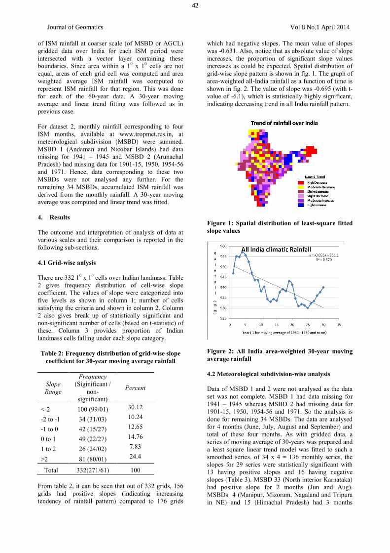
From table 2, it can be seen that out of 332 grids, 156grids had positive slopes (indicating increasingtendency of rainfall pattern) compared to 176 grids

which had negative slopes. The mean value of slopeswas -0.631. Also, notice that as absolute value of slopeincreases, the proportion of significant slope valuesincreases as could be expected. Spatial distribution ofgrid-wise slope pattern is shown in fig. 1. The graph ofarea-weighted all-India rainfall as a function of time isshown in fig. 2. The value of slope was -0.695 (with t-value of -6.1), which is statistically highly significant,indicating decreasing trend in all India rainfall pattern.

Figure 1: Spatial distribution of least-square fittedslope values

Figure 2: All India area-weighted 30-year movingaverage rainfall

4.2 Meteorological subdivision-wise analysis

Data of MSBD 1 and 2 were not analysed as the dataset was not complete. MSBD 1 had data missing for1941 – 1945 whereas MSBD 2 had missing data for1901-15, 1950, 1954-56 and 1971. So the analysis isdone for remaining 34 MSBDs. The data are analysedfor 4 months (June, July, August and September) andtotal of these four months. As with gridded data, aseries of moving average of 30-years was prepared anda least square linear trend model was fitted to such asmoothed series. of 34 x 4 = 136 monthly series, theslopes for 29 series were statistically significant with13 having positive slopes and 16 having negativeslopes (Table 3). MSBD 33 (North interior Karnataka)had positive slope for 2 months (Jun and Aug).MSBDs 4 (Manipur, Mizoram, Nagaland and Tripurain NE) and 15 (Himachal Pradesh) had 3 months

42

Journal of Geomatics Vol 8 No.1 April 2014

42

having negative slope whereas 12 (Uttaranchal) had 2months having negative slopes and remaining twomonths showing lack of trend.

From table 3, it can be seen that MSBD 8 had twostatistically significant trends (one positive and onenegative). Ten MSBD (3, 6, 13, 14, 17, 25, 26, 29, 30and 32) had one month with positive trend where asseven MSBD (5, 9, 16, 20, 24, 31 and 34) had onemonth having negative trend. Twelve MSBD (7, 10,11, 18, 19, 21, 22, 23, 27, 28, 35 and 36) did not haveany month showing trend (either positive or negative).It can be seen that first ten of these MSBDs coverstates of Orissa, Uttar Pradesh, areas in East Rajasthan,West Madhya Pradesh, Gujarat, Chhatisgarh andcoastal Andhra Pradesh. Spatially, they form inverted“U” belt starting from Gujarat going to (West andEast) Uttar Pradesh and falling to coastal AndhraPradesh. The last two represent Kerala and Lakshadeepislands.

Analysing total south-west monsoon rainfall (lastcolumn of table 3), it is observed that 9 MSBD hadstatistically significant trend (4 increasing and 5decreasing). As could be expected, MSBDs havingmultiple months of similar trend, the ISM rainfall alsoretained the pattern. MSBD 33 had positive trend andMSBD 4, 12 and 15 had negative trend. Figure 3shows the slope patterns of ISM rainfall over studyyears. It can be seen that MSBD 4, 5, 12, 15 and 20have dominant negative slopes indicating tendency fordecreased rainfall over the years. The MSBD 5, 12 and15 are dominantly mountainous region in theHimalayas. MSBD 14 has a positive trend and islocated south-west of MSBD 15 and west of MSBD12, both having decreasing pattern of rainfall.Similarly, MSBD 6 is having increasing trend and islocated west of MSBD 4 and south of MSBD 5, bothhaving decreasing pattern of ISM rainfall. MSBD 32and 33 also have increasing ISM rainfall.

Figure 3: The slope patterns of total Indian summermonsoon (ISM) rainfall during study years atmeteorological sub-division (MSBD) level

4.3 Analysis at Agroclimatic Zones

Moving to coarser level, the analysis was performed atAGCL scale also. Spatial extent of agroclimaticregions of India, as defined by Planning Commissionof India, is shown in fig. 4. As mentioned earlier, ISMrainfall at AGCL was derived from gridded data. Atthis scale, both (parametric and non-parametric)methods were used and compared. It can be seen thatAGCL 15 is composed of small islands of Andaman,Nicobar and Lakshadeep. The land portion overrepresentative 10 x 10 would be very less. It was notanalysed as the gridded data were not available overthis region. Analysis was performed for the remaining14 AGCLs. The outcome of analysis is summarized inTable 4. Perusal of Table 4 reveals that three AGCLs(1, 7 and 13) did not show any statistically significanttrend in parametric procedure. There were four AGCLs(3, 4, 10 and 11) with positive slope values where asremaining seven AGCLs had significantly negativetrend in ISM rainfall. The spatial representation isshown in figure 4. As regards comparison ofparametric and non-parametric methods, it can be seenfrom table 4 that in 12 cases there is agreementbetween the decisions of parametric and non-parametric approaches. In the remaining two cases, onemethod indicated significance and the other did not.The two methods did not show contradicting decision(one increasing and another decreasing). Thus it can beconcluded that there is good agreement the twoapproaches.

Figure 4: The trend patterns of Indian summermonsoon (ISM) rainfall over agro-climatic (AGCL)regions

4.4 Comparison of all-India rainfall derived fromgridded rainfall and MSBD data

It may be of interest to compare the all-India rainfallpatterns as obtained by two methods, namely griddedrainfall and MSBD based. Since the geographic area ofeach MSBD is known, it was possible to calculate areaweighted all India rainfall. However, since MSBD 1and 2 were not analysed, it is not proper to comparethe values of rainfall. But the correlation coefficient isa sound indicator to judge the consistency of all Indiarainfall derived from these two methods. This is shown

43

Journal of Geomatics Vol 8 No.1 April 2014

43

in fig 5. The correlation is positive and strong (r =0.86), as could be expected. However, high deviationfor 2005 rainfall needs to be investigated.

Figure 5: Scatter plot of all India rainfall by twomethods, namely gridded data and MSBD data forcommon year

4.5 Analysis in neighbouring regions (includingoceanic area)

With a view to relating spatio-temporal changes inISM over Indian land mass to adjoining region,analysis region was extended to include neighboringregion including ocean. CMAP (CPC Merged Analysisof Precipitation) data were used for the same. CMAPprovides merged dataset of precipitation derived fromsatellite, rain gauge measured and forecast fromnumerical weather prediction models (Xie and Arkin,1996; 1997). The data set is available over entire earthsurface at 2.5 deg x 2.5 deg resolution on monthlyscale from 1979 to 2011. A subset of the data set overIndian region (50 – 350 N and 650 – 1000 E) for ISMseason was extracted and analysed. Since the length ofdata series is just 33, no smoothing / filtering wasperformed. The locations of statistically significantrelationships and their values of slope are shown in fig6. It can be seen that besides a cluster of decreasingpatterns in Northeast, a bigger cluster of deceasingrainfall patterns was observed in Bay of Bengal.

Figure 6: Locations and values of statisticallysignificant ISM rainfall trend values based on 1979- 2011 analysis of CMAP data over Indian region(50 – 350 N and 650 – 1000 E)

5. Discussions

The above results indicate over-all decreasing amountof rainfall. However, this need not be looked inisolation. Parallel to the changes in the monsoonrainfall, the regional land use has also been changing(Pielke et al., 2003, 2007). The land use change overIndia in the recent decades has primarily occurred interms of urbanization (Kishtawal et al., 2009). Due tocreation of irrigation systems in first few five-yearplans of independent India, significant changes havetaken place. The moisture regime has altered and areaunder agriculture has increased. This has also led tointensive agriculture. Studies have shown thattemperature regimes of the pre- and post- agriculturalgreen revolution have different characteristics (Roy etal., 2007). Such land cover transformation can producesignificant changes in the future climate and couldaffect monsoon circulation (Feddema et al., 2005).Douglas et al. (2006, 2009) have shown thatagricultural irrigation can impact regionalevapotranspiration, surface radiative balance andmesoscale rainfall over the Indian monsoon region.Similarly, there would be effect of solar andgreenhouse gas forcing (Meehl, 2003). The impact ofland use land cover changes such as urbanization andintensification of agriculture on rainfall, thoughdifficult to quantify, needs to be taken up.

6. Conclusions

From the present study, it can be concluded that basedon the analysis of last 60 years of gridded data, there isa statistically significant decreasing trend in all IndiaISM rainfall. Northeast India is one big cluster havinghighly decreasing trend. From the analysis of MSBDdata over 110 years, a very significant decreasing trendin MSBD 4, 5, 12 and 15 and increasing trend inMSBD 6 and 33 was noticeable. The correlationcoefficient between all India rainfall by gridded dataand MSBD based data is positive and strong. However,high disagreement for 2005 rainfall needs to beinvestigated.

References

Arguez, A. and R.S. Vose (2011). The definition of thestandard WMO climate normal: The key to derivingalternative climate normals. American MeteorologicalSociety, June 2011, pp 699 – 704. (DOI:10.1175/2010BAMS2955.1)

Attri, S.D. and A. Tyagi (2010). Climate profile ofIndia. India Meteorological Department, Ministry ofEarth Sciences, New Delhi: Met Monograph No.Environment Meteorology -01/2010.

Das, P.K. (1984). The monsoons – A perspective.Indian National Science Academy, New Delhi:Perspective Report Series 4.

44

Journal of Geomatics Vol 8 No.1 April 2014

44

Douglas, E., D. Niyogi, S. Frolking, J.B. Yeluripati,R.A. Pielke Sr., N. Niyogi, C.J. Vörösmarty andMohanty, U.C. (2006). Changes in moisture andenergy fluxes due to agricultural land use andirrigation in the Indian monsoon belt. Geophys. Res.Lett., 33, L14403, doi:10.1029/2006GL026550.

Douglas, E.M., A. Beltrán-Przekurat, D. Niyogi, R.A.Pielke Sr. and C.J. Vörösmarty (2009). The impact ofagricultural intensification and irrigation on land-atmosphere interactions and Indian monsoonprecipitation - A mesoscale modeling perspective.Global and Planetary Changes, 67, 117-128.

Feddema, J.J., K.W. Oleson, G.B. Bonan, L.O.Mearns, L.E. Buja, G.A. Meehl and W.M.Washington (2005). The importance of land-coverchange in simulating future climates. Science, 310,1674-1678.

Fein, J.S. and P.L. Stephens (1987). Monsoons. WileyInterscience, Washington, D.C., 654 p.

Gadgil, S, P.N. Vinayachandran, P.A. Francis and S.Gadgil (2004). Extremes of the Indian summermonsoon rainfall, ENSO and equatorial Indian Oceanoscillation. Geophysical Research Letters 31: L12213.DOI:10.1029/2004GL019733.

Gadgil, S. (2007). The Indian monsoon. Resonance,May 2007, pp 4 -20.

Gilbert, R.O. (1987). Statistical methods forenvironmental Pollution monitoring. Van NostrandReinhold, New York.

Goswami, B.N., V. Venugopal, D. Sengupta, M.S.Madhusoodanan and P.K. Xavier (2006). Increasingtrend of extreme rain events over India in a warmingenvironment. Science, 314, 1442-1445.

IPCC (Intergovernmental Panel on Climate Change)(2007). Climate Change 2007: The physical sciencebasis: Contribution of working group I to the fourthassessment report of the Intergovernmental Panel onClimate Change, edited by S. Solomon et al., 1009 pp.,Cambridge Univ. Press, Cambridge, U. K.

Kishtawal C., D. Niyogi, M. Tewari, R.A. Pielke Sr.and M. Shepherd (2009). Urbanization signature in theobserved heavy rainfall climatology over India. Int. J.Climatol., doi:10.1002/joc.2044.

Krishna Kumar, K., B. Rajagopolan, and M.A. Cane(1999). On the weakening relationship between theIndian monsoon and ENSO. Science, 284, 2156–2159.

Mazumdar, A.B., V. Thapliyal and V.V. Patekar(2001). Onset, withdrawal and duration of southwestmonsoon. Vayu Mandal, Vol. 31, No. 1- 4, pp 64 – 68.

Meehl, G.A., W.M. Washington, T.M.L. Wigley, J.M.Arblaster and A. Dai (2003). Solar and greenhouse gasforcing and climate response in the 20th century. J.Climate, 16, 426-444.

Mooley, D.A. and B. Parthasarathy (1984).Fluctuations of All-India summer monsoon rainfallduring 1871-1978. Climatic Change, 6, 287-301.

Pai, D.S. and M. Rajeevan (2007). Indian summermonsoon onset: Variability and prediction. NationalClimate Centre, India Meteorological Department -Pune (India), National Climate Centre Research ReportNo: 4/2007.

Parthasarathy, B., K. Rupa Kumar and A.A. Munot(1991). Evidence of secular variations in Indiansummer monsoon rainfall-circulation relationships. J.Climate, 4, 927-938.

Pielke Sr., R.A., D. Niyogi, T.N. Chase and J. Eastman(2003). A new perspective on climate change andvariability: A focus on India, Invited paper to theAdvanced in Atmospheric and Oceanic Sciences, Proc.Indian National Science Academy, 69, 107 – 123.

Pielke Sr., R.A., J. Adegoke, A. Beltran-Przekurat,C.A. Hiemstra, J. Lin, U.S. Nair, D. Niyogi and T.E.Nobis (2007). An overview of regional land use andland cover impacts on rainfall. Tellus B, 59B, 587-601.

Planning Commission, (Government of India), (1989).Agro-climatic regional planning - An overview. NewDelhi, Government of India.

Rajeevan M, J. Bhate, J.D. Kale and B. Lal (2005).Development of a high resolution daily gridded rainfalldata for the Indian land region. Met. MonographClimatology No. 22/2005, Tech. rep., IMD, NationalClimate Centre, India Meteorological Department,Pune, India.

Rajeevan, M, J. Bhate, J.D. Kale and B. Lal (2006).High resolution daily gridded rainfall data for theIndian region: Analysis of break and active monsoonspells. Current Science 91:296–306.

Rajeevan, M, S. Gadgil and J. Bhate (2010). Activeand break spells of the Indian summer monsoon. J.Earth Syst. Sci. 119, No. 3, June 2010, pp. 229–247.

Roy, S.S., R. Mahmood, D. Niyogi, M. Lei, S.A.Foster, K.G. Hubbard, E. Douglas and R.A. Pielke Sr.(2007). Impacts of the agricultural green revolution-induced land use changes on air temperatures in India.J. Geophys. Res., 112, D21108,doi:10.1029/2007JD008834.

Sahai, A.K., A.M. Grimm, V. Satyan and G.B. Pant(2003). Long-lead prediction of Indian summermonsoon rainfall from global SST evolution. ClimateDynamics 20: 855–863.

45

Journal of Geomatics Vol 8 No.1 April 2014

45

Shepard, D. (1968). A two-dimensional interpolationfunction for irregularly-spaced data, ACM,Proceedings of the 23rd ACM National Conference,517 – 524, Association for Computing Machinery,New York, NY.

Srivastava, H.N., B.N. Dewan, S.K. Dikshit, G.S.Prakash Rao, S.S. Singh and K.R. Rao (1992).Decadal trends in climate over India. Mausam, 1992,43, 7–20.

WMO, (1989). Calculation of monthly and annual 30-year standard normals. WCDP- No 10, WMO – TD /No. 341, World Meteorological Organisation, Geneva.

www.metoffice.gov.uk/climate/uk/averages; (Accessedon Oct 24, 2012)

www.ncdc.noaa.gov.oa/climate/normals/usnormals.html; (Accessed on Oct 24, 2012)

www.wmo.int/pages/themes/climate/climate_data_and_products.php; (Accessed on Oct 24, 2012)

Xie, P. and P.A. Arkin (1996). Analysis of globalmonthly precipitation using gauge observations,satellite estimates, and numerical model predictions. J.Climate, 9, 840-858.

Xie, P. and P.A. Arkin (1997). Global precipitation: A17-year monthly analysis based on gauge observations,satellite estimates, and numerical model outputs. Bull.Amer. Meteor. Soc., 78, 2539-2558.

Table 3: Value of slope coefficient for 30-year moving monthly average and ISM rainfall at meteorological sub-division (MSBD) level. (Values in bold indicate statistically significant at 5 % level)

46

Journal of Geomatics Vol 8 No.1 April 2014

46

Table 4:Value of slope coefficient along with R2 and F value for 30-year moving average ISM rainfall atagro-climatic region (AGCL) level

AGCL Region Slope R2 F Remarks Z-value Remarks1 Western Himalayan -0.53 0.04 1.11 NS 0.07 NS2 Eastern Himalayan -4.64 0.44 22.6 Negative -3.88 Negative3 Lower Gangatic Plains 4.94 0.93 378.5 Positive 6.66 Positive

4 Middle Gangatic Plains 1.28 0.6 43.69 Positive 4.62 Positive

5 Upper Gangatic Plains -1.64 0.79 108.5 Negative -5.74 Negative6 Trans Gangatic Plains -1.03 0.55 34.81 Negative -4.49 Negative

7 Eastern Plateaus & Hills 0.4 0.12 4.09 NS 2.24 Positive

8 Central Plateau & hills -1.39 0.62 47.64 Negative -4.69 Negative

9 Western Plateau & hills -0.97 0.35 15.5 Negative -2.92 Negative

10 Southern Plateau &Hills

0.9 0.3 12.37 Positive 1.94 NS

11 East coast Plains & hills 1.01 0.41 20.18 Positive 2.28 Positive

12 West coast Plains &Hills

-2 0.41 20.5 Negative -3.13 Negative

13 Gujarat Plains & Hills -0.64 0.1 3.14 NS -0.24 NS14 Western Dry -0.42 0.17 5.76 Negative -2.11 Negative15 The Islands No-data

PARAMETRIC METHOD NON-PARAMETRICMETHOD

NS indicates statistically non-significant.

47

Journal of Geomatics Vol 8 No.1 April 2014

47