sparr: analyzing spatial relative risk using fixed and ... · jss journalofstatisticalsoftware...

JSS Journal of Statistical SoftwareMarch 2011, Volume 39, Issue 1. http://www.jstatsoft.org/

sparr: Analyzing Spatial Relative Risk Using Fixed

and Adaptive Kernel Density Estimation in R

Tilman M. DaviesMassey University

Martin L. HazeltonMassey University

Jonathan C. MarshallMassey University

Abstract

The estimation of kernel-smoothed relative risk functions is a useful approach to ex-amining the spatial variation of disease risk. Though there exist several options for per-forming kernel density estimation in statistical software packages, there have been veryfew contributions to date that have focused on estimation of a relative risk function perse. Use of a variable or adaptive smoothing parameter for estimation of the individualdensities has been shown to provide additional benefits in estimating relative risk andspecific computational tools for this approach are essentially absent. Furthermore, lit-tle attention has been given to providing methods in available software for any kind ofsubsequent analysis with respect to an estimated risk function. To facilitate analyses inthe field, the R package sparr is introduced, providing the ability to construct both fixedand adaptive kernel-smoothed densities and risk functions, identify statistically signifi-cant fluctuations in an estimated risk function through the use of asymptotic tolerancecontours, and visualize these objects in flexible and attractive ways.

Keywords: density estimation, variable bandwidth, tolerance contours, geographical epidemi-ology, kernel smoothing.

1. Introduction

In epidemiological studies it is often of interest to have an understanding of the dispersionof some disease within a given geographical region. A common objective in such analyses isto determine the way in which the ‘risk’ of contraction of the disease varies over the spatialarea in which the data has been collected. In order to avoid confounding by the underlyingpopulation dispersion, it is necessary to obtain not only the disease case location data, butalso control data describing this at-risk distribution. By then finding the ratio of estimatedcase to control densities (Bithell 1990, 1991), the resulting relative risk function is a commontool for describing the spatial variation in disease risk (see for example Kelsall and Diggle

http://www.jstatsoft.org/

2 sparr: Spatial Relative Risk in R

1995b; Wheeler 2007; Clough, Fenton, French, Miller, and Cook 2009).

In these and indeed most other examples, kernel smoothing is used to estimate the densities.Kernel smoothing provides a flexible approach to modeling the highly heterogeneous spatialdistributions encountered in problems in geographical epidemiology, as well as an accessibleframework for subsequent analysis. To date, the use of a fixed smoothing parameter (thatis, a constant degree of smoothing for all observations) has dominated in the literature. Afixed bandwidth is relatively simple to implement and often effective, but can perform poorlywith highly heterogeneous populations. For such distributions, the well-known variable (oradaptive) smoothing parameter method of Abramson (1982) has been shown to provide boththeoretical and practical benefits with respect to the final density estimate (Abramson 1982;Hall and Marron 1988; Davies and Hazelton 2010). It is not unreasonable to assume that theincreased complexity of the adaptive approach over the fixed, as well as the lack of specificcomputational tools for performing this kind of relative risk estimation, are at least partly toblame for the somewhat limited number of examples in the literature.

We seek to motivate further interest in this specific field by introducing the package sparr(spatial relative risk) for use with the statistical programming environment R (R Develop-ment Core Team 2010); freely available on the Comprehensive R Archive Network (CRAN)at http://CRAN.R-project.org/package=sparr. There already exist a number of packagesthat can perform bivariate kernel density/intensity estimation in R; see for example spat-stat (Baddeley and Turner 2005), ks (Duong 2007), KernSmooth (Wand and Ripley 2010)and spatialkernel (Zheng and Diggle 2011). With the exception of spatialkernel (which itselfprovides only fixed smoothing), however, none provide the explicit capability to estimate fixedand adaptive relative risk functions. In addition to this functionality, sparr also implementsthe unique ability to construct asymptotically derived p value surfaces for both fixed (Hazeltonand Davies 2009) and adaptive (Davies and Hazelton 2010) relative risk function estimates.Superimposition upon a plot of a certain risk function of tolerance contours (based on thesep values) at given significance levels can help to identify sub-regions of statistically significantdepartures from uniformity of risk; often of interest in studies in geographical epidemiol-ogy. For a further review of spatial point pattern analysis in R, see Bivand, Pebesma, andGomez-Rubio (2008).

This work is organized as follows. Section 2 gives a brief overview of the (bivariate) kerneldensity estimator (for both fixed and adaptive smoothing), discusses correction for boundarybias and outlines estimation of a relative risk function. Section 3 describes the developmentand use of asymptotic tolerance contours. Section 4 walks the reader through an analysis usingsparr and an example dealing with the spatial distribution of primary biliary cirrhosis in aregion of northeast England. Concluding remarks discussing the package and its limitations,as well as future goals, are provided in Section 5.

2. Kernel density estimation and the risk function

Consider n bivariate observations X1,X2, . . . ,Xn drawn from an unknown density f . Usingkernel smoothing, this density may then be estimated by f , given by

f(z) =1

n

n∑i=1

h−2i K

(z −Xi

hi

), (1)

http://CRAN.R-project.org/package=sparr

Journal of Statistical Software 3

where K is the kernel function, typically chosen to be a radially symmetric probability densityfunction, and hi is the smoothing parameter or bandwidth for the ith observation.

We may replace hi in (1) by some constant value hF to give us an explicit definition for thefixed-bandwidth kernel density estimator. For the adaptive estimator, we turn to an approachsuggested by Abramson (1982), and calculate the varying bandwidths by

hi = h0f(Xi)−1/2γ−1, (2)

where h0 is a secondary smoothing multiplier we refer to as the global bandwidth, and γ issimply the geometric mean of the f(Xi)

−1/2 terms, in place to alleviate the dependency ofthe his on the scale of the recorded data. The form of variable bandwidth calculation in (2) isintuitively natural since amount of smoothing depends inversely on the local amount of data.

In practice we must replace the unknown density in (2) by a pilot density. The pilot densityfh is itself a fixed-bandwidth kernel density estimate constructed with the pilot bandwidth h.

Suppose we now have not one but two sets of bivariate observations, X1,X2, . . . ,Xn1 andY 1,Y 2, . . . ,Y n2 , representing cartesian coordinates of (disease) case and control locationsrespectively. Bithell (1990, 1991) suggests that the relative risk function may be expressed asthe ratio of the (unknown) case and control densities f and g respectively. The function r istherefore written as

r(z) =f(z)

g(z). (3)

In order to symmetrize our treatment of the two densities, Kelsall and Diggle (1995a,b)advocate the use of the log-risk function ρ, where ρ = logr. Thus, by replacing f and g in(3) by their fixed or adaptive kernel estimates based on the sampled data, we obtain ourestimated (log) relative risk function (ρ = logr); r = f/g.

A common consideration in these problems is the fact that the data have been collectedover a restricted geographical region R. This is important because a portion of the kernel‘contributions’ of observations that lie near the region boundary can fall outside the definedregion. If ignored, this creates a negative bias around the boundary that can adverselyaffect the resulting density (and risk function) estimate. To correct for this by creatingan asymptotically negligible level of boundary bias, we must implement methods describedin Kelsall and Diggle (1995a) (fixed) and Marshall and Hazelton (2010) (adaptive), whichinvolves quantifying the proportion of kernel weight left within the boundary. That is, wecorrect a given density estimate f by dividing it at each location z by the value qh(z)(z), givenas

qh(z)(z) =

∫Rh−2(z)K

(x− z

h(z)

)dx, (4)

where h(z) is the bandwidth at location z. For the fixed density estimate, we recall thath(z) = hF for all z.

The R package sparr includes functions to perform the aforementioned tasks: kernel estimationof bivariate edge-corrected fixed and adaptive densities, as well as estimation of a relative riskfunction. Code examples are given in Section 4.


3. Asymptotic tolerance contours

It is often desirable in analyses involving relative risk functions to be able to identify sta-tistically significant fluctuations in the risk itself. For example, we may wish to determinewhether or not a given peak in an estimated surface reflects truly heightened risk or is simplya product of random variation. This can be thought of as an upper tailed hypothesis test.That is, for a given log relative risk function ρ, we write

H0: ρ(z) = 0HA: ρ(z) > 0.

(5)

Calculation of pointwise p values over the estimated log relative risk function ρ can be achievedwith respect to the above hypotheses. Then, we may superimpose upon a plot of ρ at givensignificance levels tolerance contours, which highlight any identified ‘extreme’ sub-regions ofelevated risk.

The question arises as to how to calculate these p value surfaces. Until recently, this was doneby Monte-Carlo (MC) permutations for fixed risk functions (see Kelsall and Diggle 1995a).However, this approach would be extremely computationally expensive for the adaptive ap-proach, and findings in Hazelton and Davies (2009) suggested that the MC tolerance contoursare prone to signify artefactual risk hotspots in areas where there are no data.

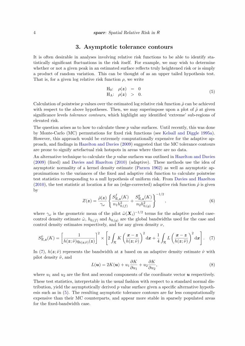
An alternative technique to calculate the p value surfaces was outlined in Hazelton and Davies(2009) (fixed) and Davies and Hazelton (2010) (adaptive). These methods use the idea ofasymptotic normality of a kernel density estimate (Parzen 1962) as well as asymptotic ap-proximations to the variances of the fixed and adaptive risk function to calculate pointwisetest statistics corresponding to a null hypothesis of uniform risk. From Davies and Hazelton(2010), the test statistic at location z for an (edge-corrected) adaptive risk function ρ is givenby

Z(z) =ρ(z)

γω

{SfR,z(K)

n1h20,(f)+SgR,z(K)

n2h20,(g)

}−1/2, (6)

where γω is the geometric mean of the pilot ω(Xi)−1/2 terms for the adaptive pooled case-

control density estimate ω, h0,(f) and h0,(g) are the global bandwidths used for the case andcontrol density estimates respectively, and for any given density ν,

S νR,z(K) =

[1

h(z; ν)qh(z;ν)(z)

]2×

[2

∫RK

(x− z

h(z; ν)

)2

dx +1

4

∫RL

(x− z

h(z; ν)

)2

dx

]. (7)

In (7), h(z; ν) represents the bandwidth at z based on an adaptive density estimate ν withpilot density ν, and

L(u) = 2K(u) + u1∂K

∂u1+ u2

∂K

∂u2, (8)

where u1 and u2 are the first and second components of the coordinate vector u respectively.

These test statistics, interpretable in the usual fashion with respect to a standard normal dis-tribution, yield the asymptotically derived p value surface given a specific alternative hypoth-esis such as in (5). The resulting asymptotic tolerance contours are far less computationallyexpensive than their MC counterparts, and appear more stable in sparsely populated areasfor the fixed-bandwidth case.


In addition to the capability of estimating fixed and adaptive risk functions, sparr includesthe functionality to produce corresponding asymptotic p value surfaces and their tolerancecontours, as well as flexible visualization options. These are put to use in the example in thefollowing section.

4. Code examples

To illustrate use of sparr we make use of a dataset concerning liver disease in a set of adjacenthealth regions in northeast England. The data, first presented and analyzed by Prince,Chetwynd, Diggle, Jarner, Metcalf, and James (2001) and included in sparr, comprise thelocations of 761 cases of primary biliary cirrhosis (PBC), along with 3020 controls randomlyselected using weighted postal zones, to represent the at-risk population. The following codeproduces Figure 1.

R> data("PBC")

R> par(mfrow = c(1, 2))

R> plot(PBC$owin, main = "cases")

R> axis(1)

R> axis(2)

Figure 1: Distribution of cases and controls, including the defining region, for the PBCdataset.


R> title(xlab = "Easting", ylab = "Northing")

R> points(PBC$data[PBC$data$ID == 1, 1:2], cex = 0.8)

R> plot(PBC$owin, main = "controls")

R> axis(1)

R> axis(2)

R> title(xlab = "Easting", ylab = "Northing")

R> points(PBC$data[PBC$data$ID == 0, 1:2], pch = 3, cex = 0.8)

R> par(mfrow = c(1, 1))

The goal is to construct an edge-corrected, adaptive (log) relative risk function; calculate anappropriate (asymptotic) p value surface searching for elevated PBC risk ‘hotspots’ (5); anddisplay and summarize the results. We note that all examples (and approximate functionrunning times) were executed on a PC desktop machine with an Intel Pentium Dual CPU at2.2Ghz, 2Gb RAM; running Microsoft Windows XP Professional.

Prior to commencing, we must decide upon the selection of appropriate bandwidths. For fixedrelative risk functions, we are required to select two bandwidths, hF1 and hF2, for the case (f)and control (g) density estimates respectively. Often, a ‘jointly optimal’ smoothing parameteris chosen for both densities when fixed estimates are used, that is hF1 = hF2 = hJ , due tocertain resultant theoretical benefits. This reduces the number of distinct values requiredto one. Adaptive density estimates, on the other hand, require both a global and pilotbandwidth. In Davies and Hazelton (2010), the authors used a common value for both caseand control global bandwidths, but left distinct the two pilot smoothing parameters. Werepeat this procedure for this example.

This leaves the issue of precisely how to calculate the required smoothing parameters. Kelsalland Diggle (1995a,b) and Hazelton (2008) suggested methods to select a common bandwidthgiven a fixed risk function (also applicable to a common global in the adaptive version),but we have found these approaches to have unreliable performance and be computationallyexpensive. Davies and Hazelton (2010) instead made use of methods designed for single densityestimates in conjunction with the pooled case/control dataset. They considered a maximalsmoothing principle suggested by Terrell (1990), as well as a least-squares cross-validationapproach available in the package sm (as summarized in Bowman and Azzalini 1997). Thesemethods have been made available in sparr.

The following R code, assuming the PBC dataset has already been loaded into the workspace,specifies bandwidths and calculates adaptive ‘pooled’, ‘case’ and ‘control’ bivariate densityestimates (information from the pooled dataset estimate is used in the analysis).

R> n1 <- sum(PBC$data$ID)

R> n2 <- nrow(PBC$data) - n1

R> pool.pilot <- CV.sm(PBC$data[,1:2])

R> pool.global <- OS(PBC$data[,1:2])

R> pbc.pool <- bivariate.density(data = PBC$data[,1:2],

+ pilotH = pool.pilot, globalH = pool.global, WIN = PBC$owin)

R> f.pilot <- CV.sm(PBC$data[PBC$data$ID == 1, 1:2])

R> g.pilot <- CV.sm(PBC$data[PBC$data$ID == 0, 1:2])

R> f.global <- g.global <- OS(PBC$data[,1:2], nstar = sqrt(n1 * n2))

R> pbc.case <- bivariate.density(data = PBC$data, ID = 1, pilotH = f.pilot,

+ globalH = f.global, WIN = PBC$owin, gamma = pbc.pool$gamma)


R> pbc.con <- bivariate.density(data = PBC$data, ID = 0, pilotH = g.pilot,

+ globalH = g.global, WIN = PBC$owin, gamma = pbc.pool$gamma)

On the previously mentioned machine, these calculations take under two minutes collectively.We are left with our adaptive density estimates based on the pooled dataset, as well as thecase and control data separately, represented as objects of class bivden (bivariate density)by sparr. This class is essentially a named list of components describing the density estimate;individual components are accessible via the familiar $ notation.

Simple S3 support in the form of print, summary and plot methods is available for thebivden class. As usual, entering the name of a stored object within the current workspacewill invoke the relevant print command, the appearance of which is seen for the ‘case’ densityobject below.

R> pbc.case

Bivariate kernel density estimate

Adaptive isotropic smoothing with (pilot) h = 494.2531 global h = 349.8445

unit(s)

No. of observations: 761

We are now ready to calculate a (log) relative risk function; a trivial task in sparr throughthe use of the function risk. This method produces a named list object of the class rrs, forwhich the same S3 support is available as described above.

R> pbc.risk <- risk(f = pbc.case, g = pbc.con, plotit = FALSE)

R> summary(pbc.risk)

Log-Relative risk function.

Surface (Z) summary:

Min. 1st Qu. Median Mean 3rd Qu. Max. NA's

-2.7810 -1.1610 -0.7845 -0.7742 -0.3453 0.9925 1147.0000

--Numerator (case) density--



unit(s)


Evaluated over 50 by 50 rectangular grid.

Defined study region is a polygon with 115 vertices.

Estimated density description


3.182e-11 6.104e-10 1.205e-09 1.238e-08 8.141e-09 3.967e-07 1.147e+03


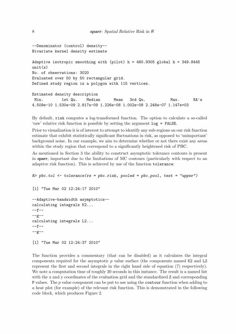
--Denominator (control) density--



unit(s)


Evaluated over 50 by 50 rectangular grid.

Defined study region is a polygon with 115 vertices.

Estimated density description


4.509e-10 1.530e-09 2.817e-09 1.226e-08 1.002e-08 2.248e-07 1.147e+03

By default, risk computes a log-transformed function. The option to calculate a so-called‘raw’ relative risk function is possible by setting the argument log = FALSE.

Prior to visualization it is of interest to attempt to identify any sub-regions on our risk functionestimate that exhibit statistically significant fluctuations in risk, as opposed to ‘unimportant’background noise. In our example, we aim to determine whether or not there exist any areaswithin the study region that correspond to a significantly heightened risk of PBC.

As mentioned in Section 3 the ability to construct asymptotic tolerance contours is presentin sparr; important due to the limitations of MC contours (particularly with respect to anadaptive risk function). This is achieved by use of the function tolerance:

R> pbc.tol <- tolerance(rs = pbc.risk, pooled = pbc.pool, test = "upper")

[1] "Tue Mar 02 12:24:17 2010"

--Adaptive-bandwidth asymptotics--

calculating integrals K2...

--f--

--g--

calculating integrals L2...

--f--

--g--

[1] "Tue Mar 02 12:24:37 2010"

The function provides a commentary (that can be disabled) as it calculates the integralcomponents required for the asymptotic p value surface (the components named K2 and L2

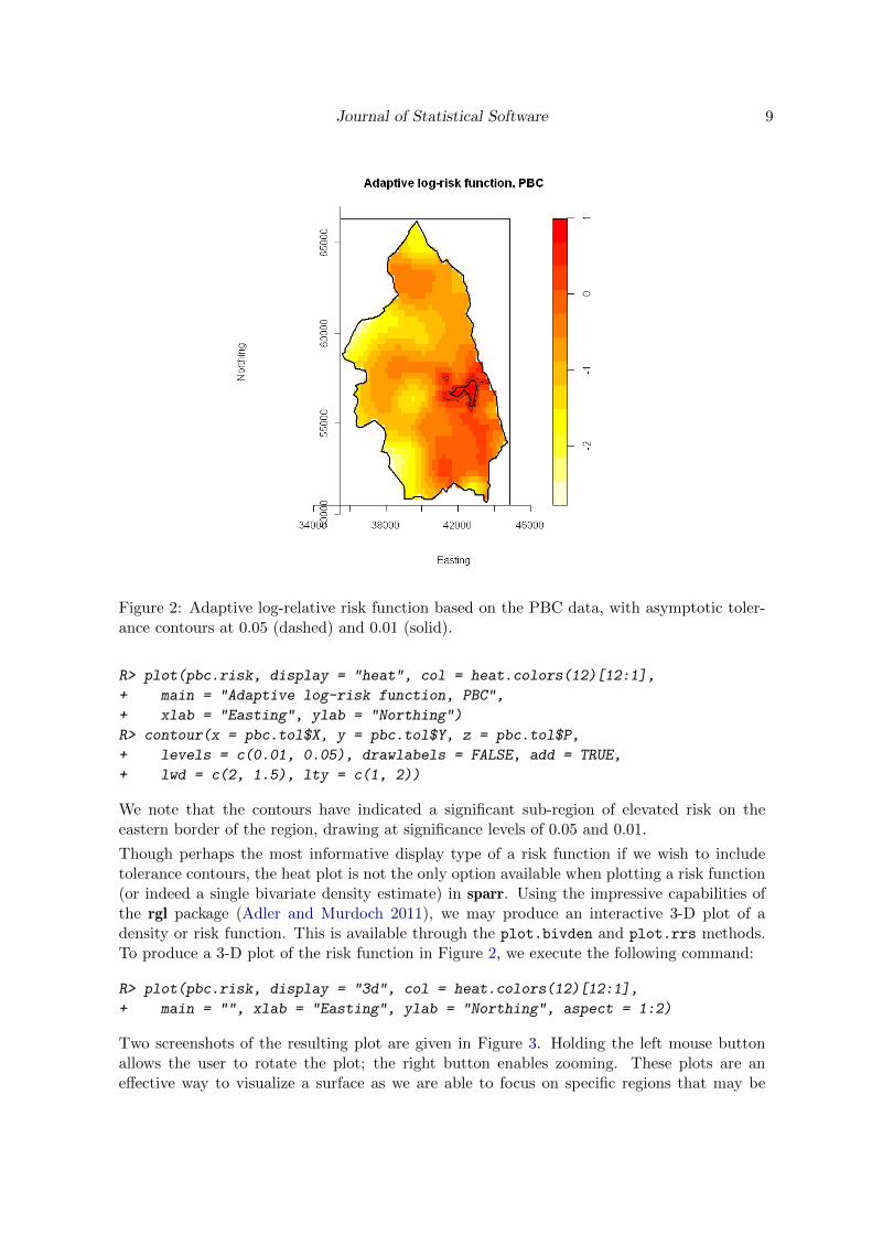
represent the first and second integrals in the right hand side of equation (7) respectively).We note a computation time of roughly 20 seconds in this instance. The result is a named listwith the x and y coordinates of the evaluation grid and the standardized Z and correspondingP values. The p value component can be put to use using the contour function when adding toa heat plot (for example) of the relevant risk function. This is demonstrated in the followingcode block, which produces Figure 2.


Figure 2: Adaptive log-relative risk function based on the PBC data, with asymptotic toler-ance contours at 0.05 (dashed) and 0.01 (solid).

R> plot(pbc.risk, display = "heat", col = heat.colors(12)[12:1],

+ main = "Adaptive log-risk function, PBC",

+ xlab = "Easting", ylab = "Northing")

R> contour(x = pbc.tol$X, y = pbc.tol$Y, z = pbc.tol$P,

+ levels = c(0.01, 0.05), drawlabels = FALSE, add = TRUE,

+ lwd = c(2, 1.5), lty = c(1, 2))

We note that the contours have indicated a significant sub-region of elevated risk on theeastern border of the region, drawing at significance levels of 0.05 and 0.01.

Though perhaps the most informative display type of a risk function if we wish to includetolerance contours, the heat plot is not the only option available when plotting a risk function(or indeed a single bivariate density estimate) in sparr. Using the impressive capabilities ofthe rgl package (Adler and Murdoch 2011), we may produce an interactive 3-D plot of adensity or risk function. This is available through the plot.bivden and plot.rrs methods.To produce a 3-D plot of the risk function in Figure 2, we execute the following command:

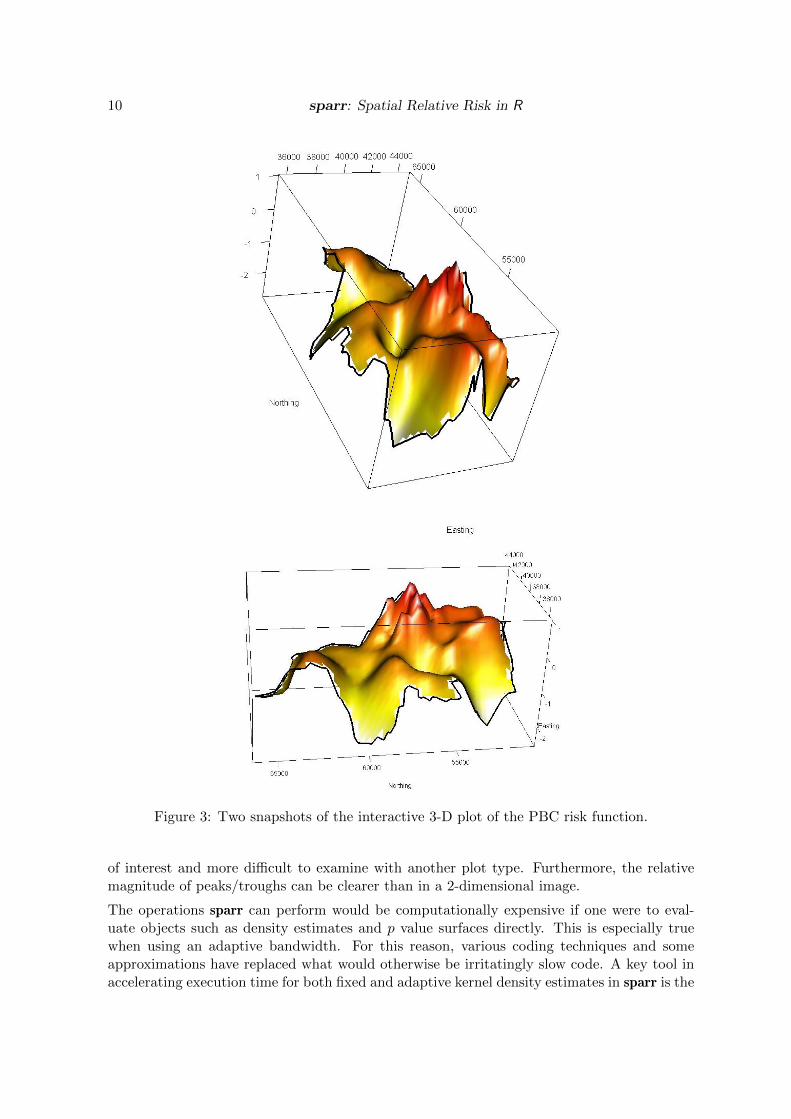
R> plot(pbc.risk, display = "3d", col = heat.colors(12)[12:1],

+ main = "", xlab = "Easting", ylab = "Northing", aspect = 1:2)

Two screenshots of the resulting plot are given in Figure 3. Holding the left mouse buttonallows the user to rotate the plot; the right button enables zooming. These plots are aneffective way to visualize a surface as we are able to focus on specific regions that may be


Figure 3: Two snapshots of the interactive 3-D plot of the PBC risk function.

of interest and more difficult to examine with another plot type. Furthermore, the relativemagnitude of peaks/troughs can be clearer than in a 2-dimensional image.

The operations sparr can perform would be computationally expensive if one were to eval-uate objects such as density estimates and p value surfaces directly. This is especially truewhen using an adaptive bandwidth. For this reason, various coding techniques and someapproximations have replaced what would otherwise be irritatingly slow code. A key tool inaccelerating execution time for both fixed and adaptive kernel density estimates in sparr is the


powerful Fast-Fourier Transform code used to evaluate edge-corrected fixed-bandwidth densityestimates in spatstat (via its function density.ppp). Though this is a trivial translation forbivariate.density to make for the fixed bandwidth case, more thought is required to utilizethe advantageous speed of the spatstat code for adaptive estimation, where we require band-widths for all possible grid coordinates to edge-correct. In this situation, bivariate.densitycalculates these bandwidths and finds the unique values of the 100 integer quantiles thereof.Each of these unique values is then treated as a fixed bandwidth, and the corresponding fixed-bandwidth edge-correction factors are extracted from the Fast-Fourier Transform-calculatedobjects. A given coordinate within the study region is then matched to the nearest appropriateinteger quantile value by its bandwidth, and the edge-correction factor corresponding to thatbandwidth and coordinate is assigned. This approximation is significantly faster than directlyevaluating factors at each distinct coordinate and associated bandwidth, at a negligible costof accuracy. Nevertheless, the user can turn off the option to use this Fast-Fourier Transformassistance by setting the bivariate.density argument use.ppp.methods = FALSE. Otherapproximations of note are made for the integral components of the asymptotic p value sur-faces in tolerance, again using the Fast-Fourier methods of spatstat as well as approachesthat involve single evaluations of a function, translated to all possible grid coordinates. Seethe documentation pages for bivariate.density and tolerance for further information.

In addition, it is worth noting that a reduction in computation time may be had by reducingthe resolution of the grid over which we estimate the density or p value surface. The defaultresolution is to use a 50 by 50 grid, which we consider to be a suitable minimum resolution thatprovides serviceable estimates and images, while keeping computation costs at a relativelylow level. The user may find that a modest increase in resolution may be warranted foraesthetic reasons. In the interests of flexibility it is possible, for example, to evaluate ap value surface over a coarser grid than the corresponding risk function density estimates.This allows tolerance counters to be computed relatively quickly, and then superimposed overa more aesthetically pleasing image of the risk surface.

Finally, we mention that the complexity of the polygon describing the study region can,in extreme cases, result in a prohibitive computational cost for density and p value surfaceestimation. A polygon with many thousands of vertices (e.g. one obtained from a detailedgeographical map) will cause delays, particularly when the complex region needs to be checkedby the function multiple times for calculation of edge-correction factors. We recommend usersworking with such regions reduce the order of the polygon by, for example, retaining onlyevery kth vertex. Analysis can then be performed at a generally negligible cost of accuracy(depending on the magnitude of k) using the reduced polygon. For imaging, the researcherscan easily display the efficiently computed results using the original geographical map.

5. Final comments

Though concentrating on one particular approach for analyzing the spatial dispersion of dis-ease, we hope that sparr will prove a useful tool for epidemiologists and researchers workingwith point process case-control data in geographical epidemiology. The functions in this pack-age are flexible in the types of arguments they accept and the user can tailor their analysesto a varying level of detail. Indeed, by accepting a number of default values, the user is ableto directly estimate a relative risk function by supplying the raw data to risk, bypassing theneed to run bivariate.density explicitly.


Though there exist several packages for R that perform kernel density estimation, none (todate) provide the capabilities found here, particularly with the use of the variable bandwidth.With sparr (version 0.2-0 at the time of writing) the user is provided with flexible functions toperform fixed and adaptive bivariate kernel density estimation, including boundary correctionwith respect to a complex study region, for both smoothing regimens. In addition, the usercan calculate a relative risk function and use asymptotic theory to calculate correspondingp value surfaces and tolerance contours. Finally, sparr provides simple-to-use yet powerfulapproaches to visualizing the results.

The advancements in this package would not be possible without several other importantcontributions to CRAN; these are reflected as sparr’s package dependencies. As alreadymentioned, rgl by Adler and Murdoch (2011) provides the ability to plot in 3 dimensionsand interact with the device. The comprehensive spatial point pattern package spatstat (seeBaddeley and Turner 2005) provides functions to enable efficient region handling, as well asthe aforementioned Fast-Fourier Transform implementation. Package sm provides access tothe LSCV bandwidth selector; named CV.sm here. The base package MASS (see Venablesand Ripley 2002) provides utility support for internal functions.

There remains scope for further extensions to sparr. The issue of bandwidth selection is adifficult problem with respect to risk functions, and the somewhat ad hoc approach takenby most authors (present included) in tackling practical applications of the methodologyhas shifted the focus of sparr to the actual implementation and analysis of a risk function.Though, as mentioned, the package does provide the functionality of two bandwidth selectorsfor density estimation (OS and CV.sm), sparr generally aims to leave the bandwidth choice(s)for risk functions up to the user.

As almost all practical applications of the methodology use the Gaussian kernel function, thisis the only kernel currently supported for the bivariate kernel density estimation in sparr. Theinfinite tails of this kernel are useful in areas of a given region with sparse observations, wherea bounded kernel can result in a discontinuous estimate. Future versions of this package will,however, endeavor to expand the available choices for K.

Finally, it is worth noting the ever-present computational demands of estimating a kernel-smoothed relative risk function. Producing adaptive over fixed estimates will increase thiscost. The size of the dataset, opting to edge-correct, as well as grid resolution, also impact onexecution time. Though sparr has sought to minimize this cost as much as possible for initialrelease, it remains up to the user to find an acceptable balance between the aforementionedissues and computing time for their projects.

Acknowledgments

The authors would like to acknowledge Dr. Geoff Jones (Senior Lecturer, Dept. of Statistics,Massey University) who facilitated proofing and testing of sparr. We also thank Prof. PeterJ. Diggle (Division of Medicine, Lancaster University) for kindly providing the PBC datasetin sparr (see also http://www.lancs.ac.uk/staff/diggle/pointpatterns/Datasets/).

We thank two anonymous reviewers for providing helpful comments leading to an improvementin the presentation of this work.

T.M.D. is financially supported by a Top Achiever’s Doctoral Research Scholarship from theNew Zealand Tertiary Education Commission (TEC).

http://www.lancs.ac.uk/staff/diggle/pointpatterns/Datasets/


References

Abramson IS (1982). “On Bandwidth Estimation In Kernel Estimates – A Square Root Law.”The Annals of Statistics, 10(4), 1217–1223.

Adler D, Murdoch D (2011). rgl: 3D Visualization Device System (OpenGL). R packageversion 0.92.798, URL http://CRAN.R-project.org/package=rgl.

Baddeley A, Turner R (2005). “spatstat: An R Package for Analyzing Spatial Point Patterns.”Journal of Statistical Software, 12(6), 1–42. URL http://www.jstatsoft.org/v12/i06/.

Bithell JF (1990). “An Application of Density Estimation to Geographical Epidemiology.”Statistics in Medicine, 9, 691–701.

Bithell JF (1991). “Estimation of Relative Risk Functions.” Statistics in Medicine, 10, 1745–1751.

Bivand RS, Pebesma EJ, Gomez-Rubio V (2008). Applied Spatial Data Analysis with R.Springer-Verlag, New York. ISBN 978-0-387-78170-9.

Bowman AW, Azzalini A (1997). Applied Smoothing Techniques for Data Analysis: TheKernel Approach with S-PLUS Illustrations. Oxford University Press, New York. ISBN0-19-852396-3.

Clough HE, Fenton SE, French NP, Miller AJ, Cook AJC (2009). “Evidence from the UKZoonoses Action Plan in Favour of Localised Anomalies of Salmonella Infection on UnitedKingdom Pig Farms.” Preventive Veterinary Medicine, 89(1-2), 67–74.

Davies TM, Hazelton ML (2010). “Adaptive Kernel Estimation of Spatial Relative Risk.”Statistics in Medicine, 29(23), 2423–2437.

Duong T (2007). “ks: Kernel Density Estimation and Kernel Discriminant Analysis forMultivariate Data in R.” Journal of Statistical Software, 21(7), 1–16. URL http://www.

jstatsoft.org/v21/i07/.

Hall P, Marron JS (1988). “Variable Window Width Kernel Density Estimates of ProbabilityDensities.” Probability Theory and Related Fields, 80, 37–49.

Hazelton ML (2008). “Letter to the Editor: Kernel Estimation of Risk Surfaces Without theNeed for Edge Correction.” Statistics in Medicine, 27, 2269–2272.

Hazelton ML, Davies TM (2009). “Inference Based on Kernel Estimates of the Relative RiskFunction in Geographical Epidemiology.” Biometrical Journal, 51, 98–109.

Kelsall JE, Diggle PJ (1995a). “Kernel Estimation of Relative Risk.” Bernoulli, 1, 3–16.

Kelsall JE, Diggle PJ (1995b). “Non-Parametric Estimation of Spatial Variation in RelativeRisk.” Statistics in Medicine, 14, 2335–2342.

Marshall JC, Hazelton ML (2010). “Boundary Kernels for Adaptive Density Estimators onRegions with Irregular Boundaries.” Journal of Multivariate Analysis, 101, 949–963.

http://CRAN.R-project.org/package=rgl

http://www.jstatsoft.org/v12/i06/




Parzen E (1962). “On Estimation of a Probability Density Function and Mode.” Annals ofMathematical Statistics, 33, 1065–1076.

Prince MI, Chetwynd A, Diggle PJ, Jarner M, Metcalf JV, James OFW (2001). “The Geo-graphical Distribution of Primary Biliary Cirrhosis in a Well-Defined Cohort.” Hepatology,34, 1083–1088.

R Development Core Team (2010). R: A Language and Environment for Statistical Computing.R Foundation for Statistical Computing, Vienna, Austria. ISBN 3-900051-07-0, URL http:

//www.R-project.org/.

Terrell GR (1990). “The Maximal Smoothing Principle in Density Estimation.” Journal ofthe American Statistical Association, 85, 470–477.

Venables WN, Ripley BD (2002). Modern Applied Statistics with S. 4th edition. Springer-Verlag, New York.

Wand MP, Ripley BD (2010). KernSmooth: Functions for Kernel Smoothing for Wand& Jones (1995). R package version 2.23-4, URL http://CRAN.R-project.org/package=

KernSmooth.

Wheeler DC (2007). “A Comparison of Spatial Clustering and Cluster Detection Techniquesfor Childhood Leukemia Incidence in Ohio, 1996–2003.” International Journal of HealthGeographics, 6(13).

Zheng P, Diggle PJ (2011). spatialkernel: Nonparameteric Estimation of Spatial Segregationin a Multivariate Point Process. R package version 0.4-10, URL http://CRAN.R-project.

org/package=spatialkernel.

Affiliation:

Tilman M. DaviesDepartment of StatisticsInstitute of Fundamental SciencesMassey UniversityPalmerston North, New ZealandE-mail: [email protected]: http://ifs.massey.ac.nz/people/staff.php?personID=232

Journal of Statistical Software http://www.jstatsoft.org/

published by the American Statistical Association http://www.amstat.org/

Volume 39, Issue 1 Submitted: 2010-05-02March 2011 Accepted: 2010-08-10

http://www.R-project.org/

http://www.R-project.org/

http://CRAN.R-project.org/package=KernSmooth

http://CRAN.R-project.org/package=KernSmooth

http://CRAN.R-project.org/package=spatialkernel

http://CRAN.R-project.org/package=spatialkernel

mailto:[email protected]

http://ifs.massey.ac.nz/people/staff.php?personID=232

http://www.jstatsoft.org/

http://www.amstat.org/

sparr: analyzing spatial relative risk using fixed and ... · jss journalofstatisticalsoftware...

Documents