Some applications of MUMPs in Some applications of MUMPs in computational fluid dynamics and computational fluid dynamics and

electromagneticselectromagnetics

Al dAl d G lf tG lf tAlexander Alexander GelfgatGelfgatSchool of Mechanical School of Mechanical Engineering, Faculty Engineering, Faculty of Engineeringof Engineering

TelTel--Aviv UniversityAviv University

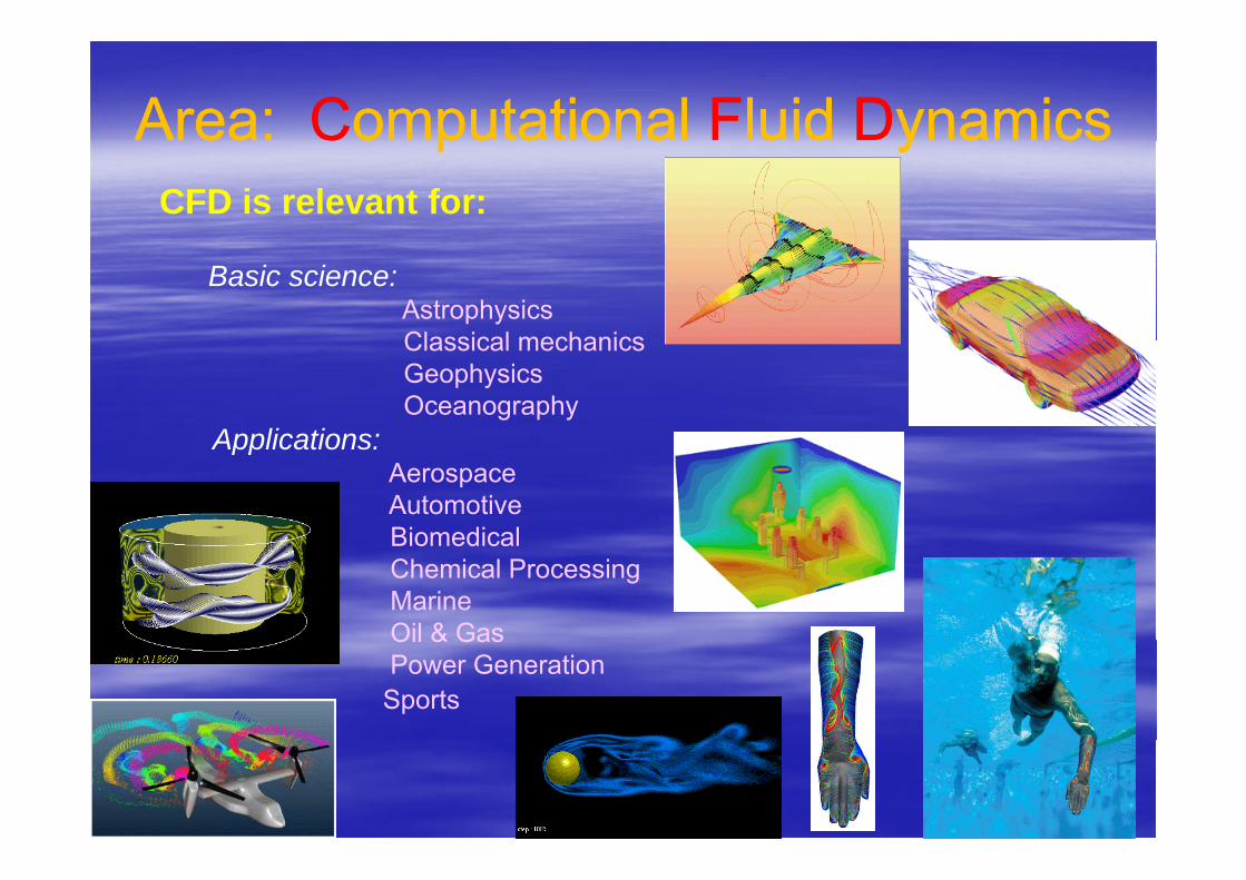
Area: Area: CComputational omputational FFluid luid DDynamicsynamicseaea CCo pu a o ao pu a o a u du d y a csy a csCFD is relevant for:

Basic science:AstrophysicsClassical mechanicsClassical mechanicsGeophysicsOceanography

Applications:Applications:AerospaceAutomotiveBiomedicalBiomedicalChemical ProcessingMarineOil & GasOil & GasPower GenerationSports

Our current project:Our current project:spiraling growth of rarespiraling growth of rare earthearth scandatesscandatesspiraling growth of rarespiraling growth of rare--earth earth scandatesscandates

caused by melt flow instabilitiescaused by melt flow instabilities

GdScO3DyScO3 SmScO3 NdScO3

2

0.5

1

1.5

Z

0

-1

-0.5

0

0.5

1

X

-1

-0.5

0

0.5

1

Y

Some historySome history

Some historySome history"Observe the motion of the surface of the waterObserve the motion of the surface of the water,which resembles that of hair, which has twomotions, of which one is caused by the weight ofthe hair, the other by the direction of the curls;thus the water has eddying motions one part ofthus the water has eddying motions, one part ofwhich is due to the principal current, the other tothe random and reverse motion.“ Leonardo daVinci, translated by Ugo Piomelli, University ofMaryland)Maryland),

1452-1519

, , ' ,t t t v r v r v r

1, ,t T

t t dt

v r v r , ,t

t t dtT v r v r

' , , ,t t t v r v r v r

Osborne Reynolds,1842-1921

, , ,t t tv v v

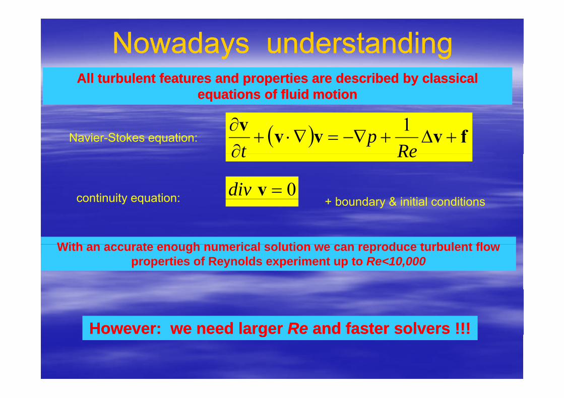
Nowadays understandingNowadays understandingAll turbulent features and properties are described by classical All turbulent features and properties are described by classical

equations of fluid motionequations of fluid motion

Navier-Stokes equation: fvvvv

Rep

t1

+ b d & i iti l diticontinuity equation:

Ret

0vdiv+ boundary & initial conditionscontinuity equation:

With t h i l l ti d t b l t flWith an accurate enough numerical solution we can reproduce turbulent flow properties of Reynolds experiment up to Re<10,000

However: we need larger However: we need larger ReRe and faster solvers !!!and faster solvers !!!gg

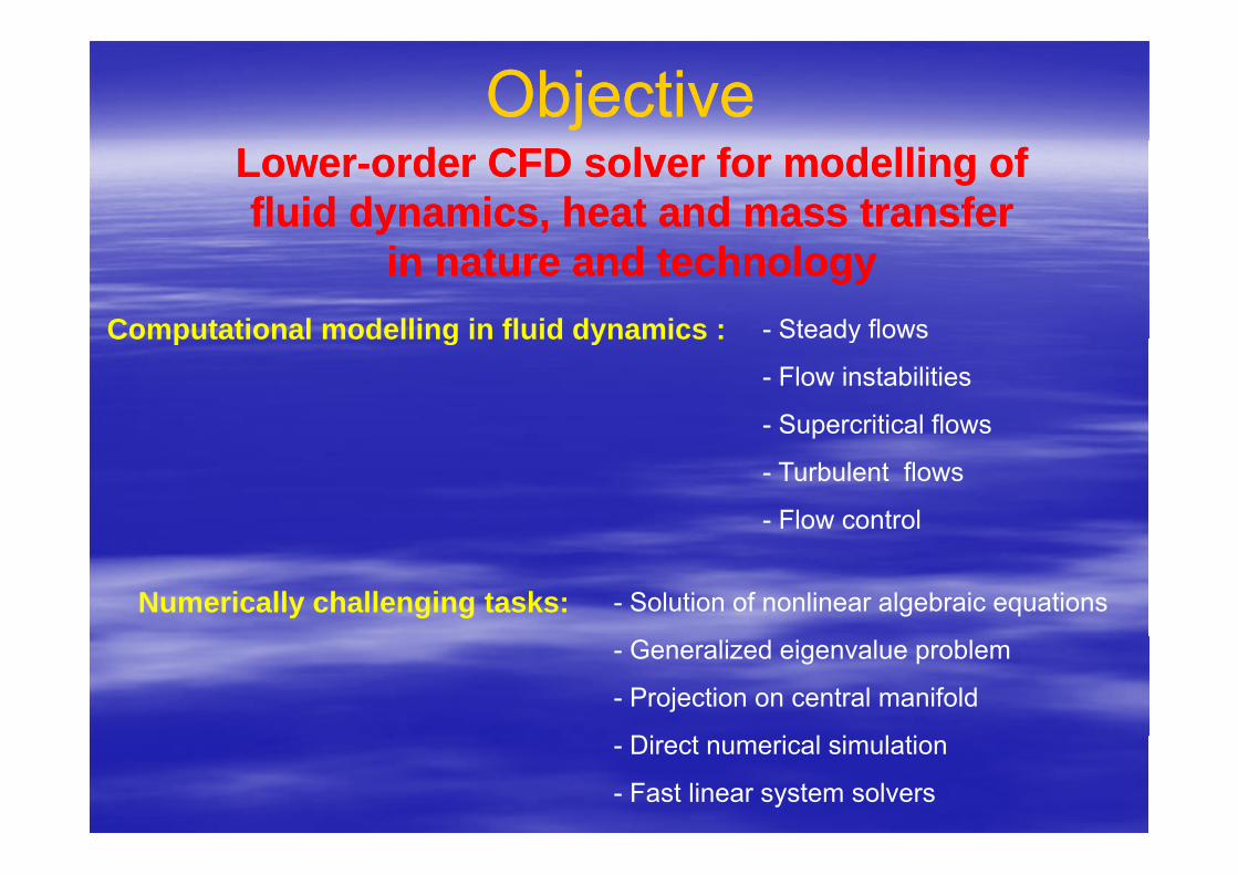
ObjectiveObjectiveLowerLower--order CFD solver for order CFD solver for modellingmodelling of of fluid dynamics, heat and mass transfer fluid dynamics, heat and mass transfer

Computational modelling in fluid dynamics : - Steady flows

in nature and technologyin nature and technologyComputational modelling in fluid dynamics : y

- Flow instabilities

- Supercritical flows p

- Turbulent flows

- Flow control

Numerically challenging tasks: - Solution of nonlinear algebraic equations

- Generalized eigenvalue problem

- Projection on central manifold

Di i l i l i- Direct numerical simulation

- Fast linear system solvers

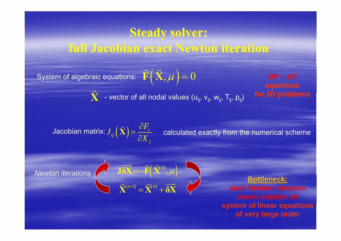
Steady solver: Steady solver: yyfull Jacobian exact Newton iteration full Jacobian exact Newton iteration

, 0 F X

System of algebraic equations:

101055 –– 101077

equations equations forfor 22D problemsD problemsX - vector of all nodal values (uij, vij, wij, Tij, pij) for for 22D problemsD problems

Jacobian matrix: iij

j

FJX

X

calculated exactly from the numerical scheme

Newton iterations: ,n JδX F X

Newton iterations:

1n n

X X δX

Bottleneck:each Newton iteration

needs solution of f li isystem of linear equations

of very large order

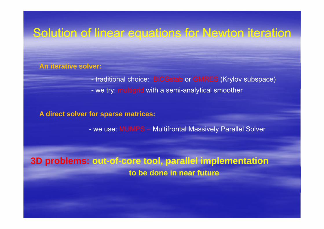
Solution of linear equations for Newton iterationSolution of linear equations for Newton iterationSolution of linear equations for Newton iterationSolution of linear equations for Newton iteration

An iterative solver:

- traditional choice: BiCGstab or GMRES (Krylov subspace)t lti id ith i l ti l th- we try: multigrid with a semi-analytical smoother

A direct solver for sparse matrices:A direct solver for sparse matrices:

- we use: MUMPS – Multifrontal Massively Parallel Solver

3D problems: out-of-core tool, parallel implementationto be done in near future

Eigenproblem for analysis of instabilitiesEigenproblem for analysis of instabilities

u uv v

Generalized eigenvalue problemwhere J is the Jacobian matrix and detB=0

w wp p

B J

Solution: Arnoldi iteration in the shift-and-invert mode

1 1, , , , , , ,T T

u v w p u v w p

J B B

Solution: Arnoldi iteration in the shift and invert mode

Choose as close as possible to the leading eigenvalue and calculate several with the largest ||.

Bottleneck: calculation of the Krylov basis 1 2, , ,..., nx x x x J B J B J B

The matrix (J−B) is iteration independent !

Calculation of LU-decomposition of (J−B)resolves the bottleneck ! Instead of an iterative solver use resolves the bottleneck ! a direct solver (we use MUMPS in

a complex mode)

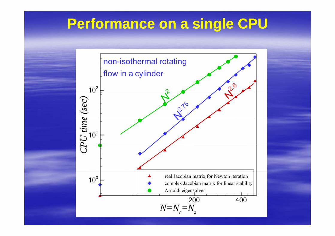
Performance on a single CPUPerformance on a single CPU

non-isothermal rotating

102

N2.6

gflow in a cylinder

2e

(sec

)10

N2

N2.75

N2

PUtim

e

101

N

CP

200 400

100 real Jacobian matrix for Newton iterationcomplex Jacobian matrix for linear stabilityArnoldi eigensolver

N=Nr=Nz

200 400

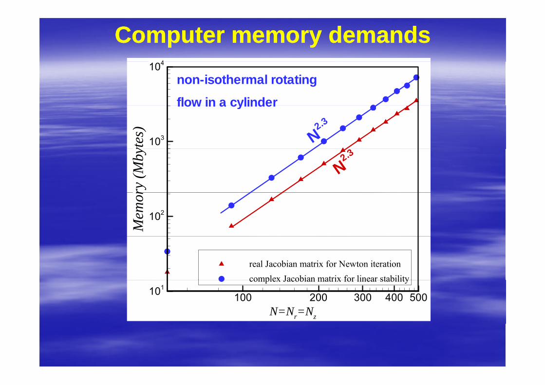
Computer memory demandsComputer memory demands4104

non-isothermal rotating

flow in a cylinder

ytes

)103

3

flow in a cylinder

N2.3

ry(M

by

N2.3

Mem

or

102

real Jacobian matrix for Newton iterationcomplex Jacobian matrix for linear stability

N=Nr=Nz

100 200 300 400 500101complex Jacobian matrix for linear stability

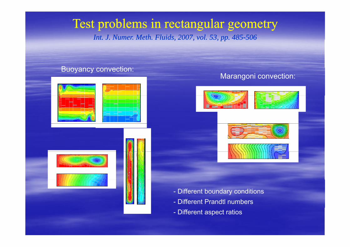
Test problems in rectangular geometryTest problems in rectangular geometryInt. J.Int. J. NumerNumer. Meth. Fluids,. Meth. Fluids, 20072007, vol., vol. 5353, pp., pp. 485485--506506Int. J. Int. J. NumerNumer. Meth. Fluids, . Meth. Fluids, 20072007, vol. , vol. 5353, pp. , pp. 485485 506506

B tiBuoyancy convection:Marangoni convection:

- Different boundary conditions- Different Prandtl numbers- Different aspect ratios

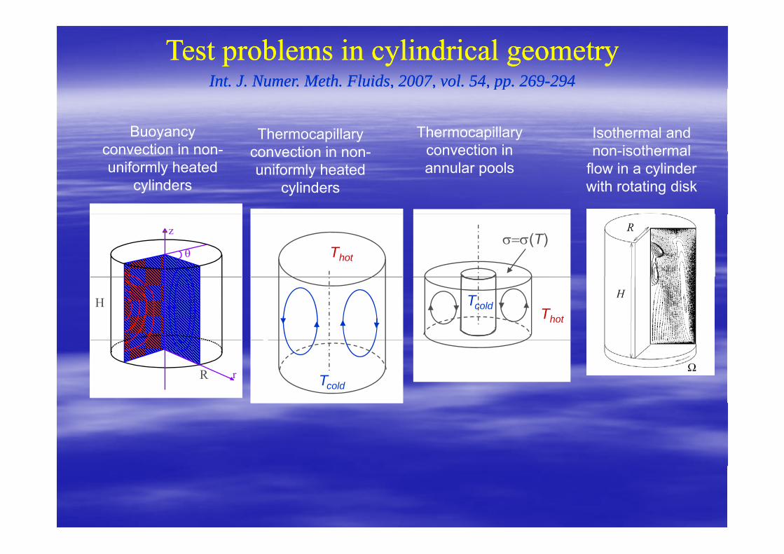
Test problems in cylindrical geometryTest problems in cylindrical geometryInt. J. Int. J. NumerNumer. Meth. Fluids, . Meth. Fluids, 20072007, vol. , vol. 5454, pp. , pp. 269269--294294pppp

Buoyancy convection in non-

Thermocapillary convection in non

Isothermal and non-isothermal

Thermocapillary convection inconvection in non

uniformly heated cylinders

convection in non-uniformly heated

cylinders

non-isothermal flow in a cylinder with rotating disk

convection in annular pools

z

Thot

(T)

H

(

T) Tcold Thot

rR Tcold

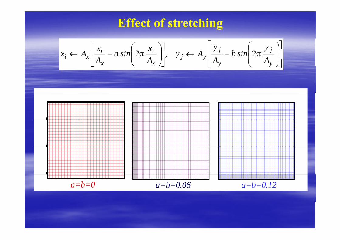
Effect of stretching Effect of stretching

y

j

y

jyj

x

i

x

ixi A

ysinb

Ay

Ay,Axsina

AxAx 22

yy

a=b=0.06 a=b=0.12a=b=0

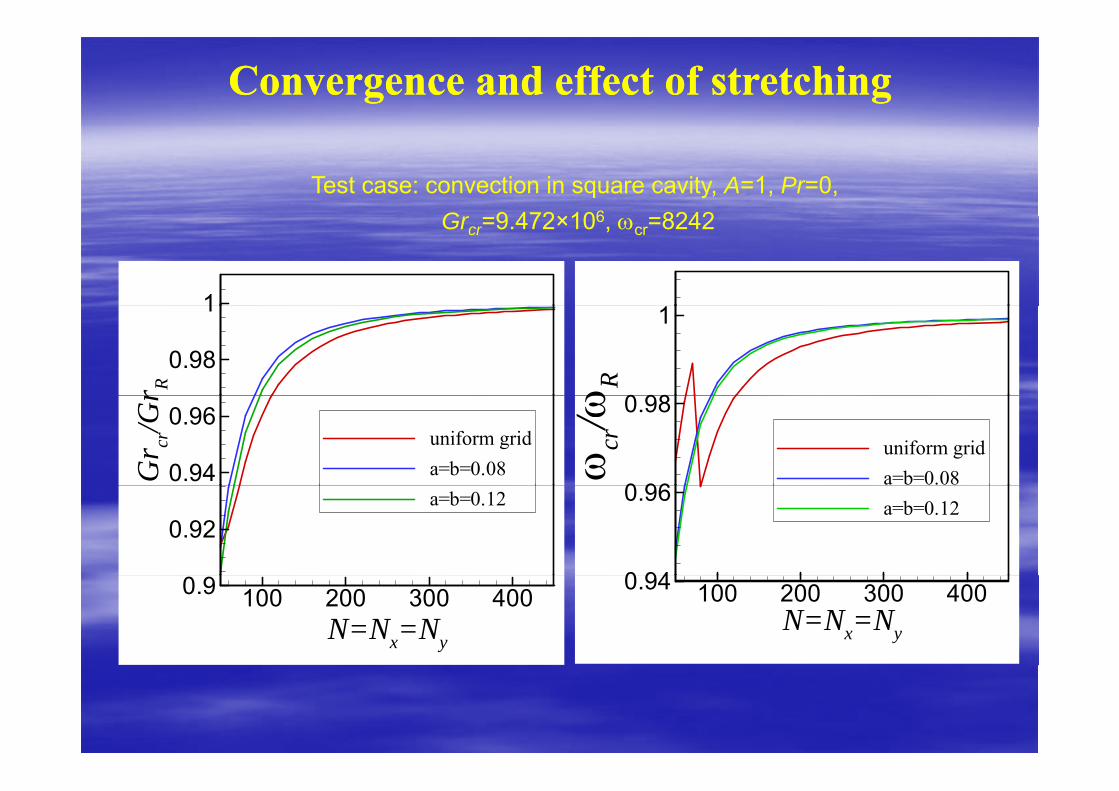
Convergence and effect Convergence and effect of stretching of stretching

Test case: convection in square cavity, A=1, Pr=0, G 9 472×106 8242Grcr=9.472×106, cr=8242

1

r R

0.98

1

R

0 98

1

Gr cr

/Gr

0.94

0.96uniform grida=b=0.08

cr/

0 96

0.98

uniform grida=b=0.08

0.92a=b=0.12

0 94

0.96a=b=0.12

N=Nx=Ny

100 200 300 4000.9N=Nx=Ny

100 200 300 4000.94

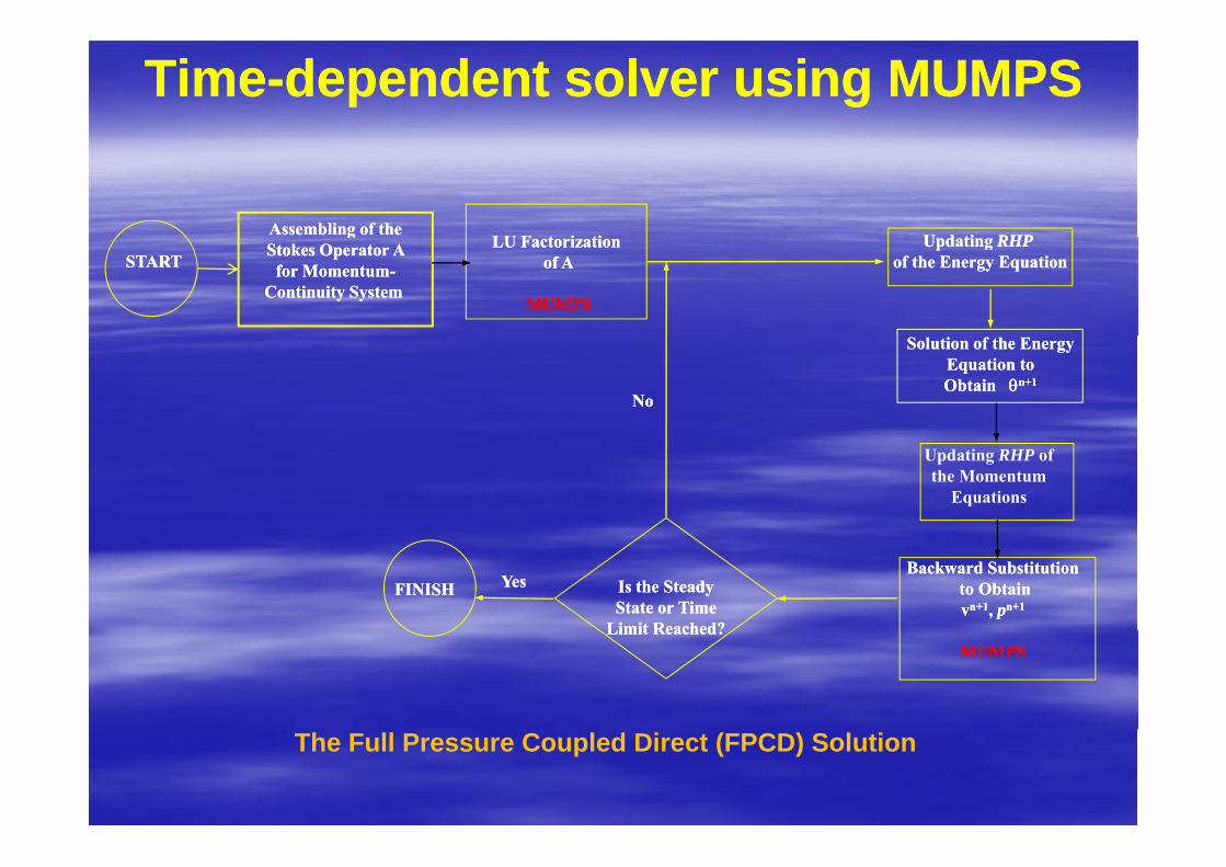
TimeTime--dependent solver using MUMPSdependent solver using MUMPS

Assembling Assembling of of the the LU F t i tiLU F t i ti U d tiU d ti RHPRHP

STARTSTART

ggStokes Operator Stokes Operator A A

for Momentumfor Momentum--Continuity System Continuity System

LU Factorization LU Factorization of Aof A

MUMPSMUMPS

Updating Updating RHPRHPof the of the EEnergy Equationnergy Equation

Solution of the Energy Solution of the Energy Equation toEquation toObtain Obtain n+n+11

NoNo

Updating RHP of the Momentum

Equations

Backward SubstitutionBackward Substitutionto to ObtainObtainvvn+n+11, , ppn+n+11

Is the Steady Is the Steady State or Time State or Time

Limit Reached?Limit Reached?

YesYesFINISHFINISH

MUMPSMUMPSLimit Reached?Limit Reached?

The Full Pressure Coupled Direct (FPCD) Solution

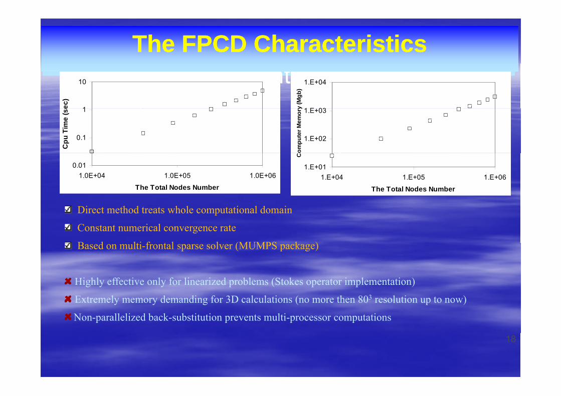
An efficient 3D time marching solver The FPCD CharacteristicsThe FPCD Characteristics(Cont.1)

1

10

ec)

1 E 03

1.E+04

y (M

gb)

10-6 ×N 1.09480.0015×N 1.0501

0.1

1

Cpu

Tim

e (s

e

1.E+02

1.E+03

ompu

ter M

emor

y

0.011.0E+04 1.0E+05 1.0E+06

The Total Nodes Number

1.E+011.E+04 1.E+05 1.E+06

The Total Nodes Number

C

Direct method treats whole computational domain

Constant numerical convergence rate

B d lti f t l l (MUMPS k )Based on multi-frontal sparse solver (MUMPS package)

Highly effective only for linearized problems (Stokes operator implementation)

Extremely memory demanding for 3D calculations (no more then 803 resolution up to now)

Non-parallelized back-substitution prevents multi-processor computations

18

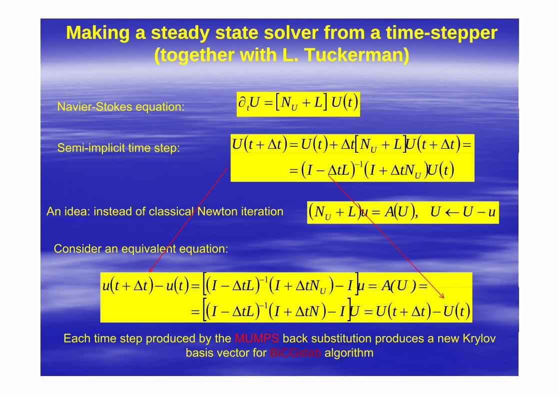
Making a steady state solver from a timeMaking a steady state solver from a time--stepper stepper (together with L. Tuckerman)(together with L. Tuckerman)( g )( g )

Navier-Stokes equation: tULNU Ut Navier-Stokes equation: Ut

Semi-implicit time step: ttULNttUttU U p p tUtNItLI U

U

1

An idea: instead of classical Newton iteration uUU,UAuLNU

Consider an equivalent equation:

)U(AuItNItLItuttu 1 tUttUUItNItLI

)U(AuItNItLItuttu U

1

Each time step produced by the MUMPS back substitution produces a new Krylov basis vector for BiCGstab algorithm

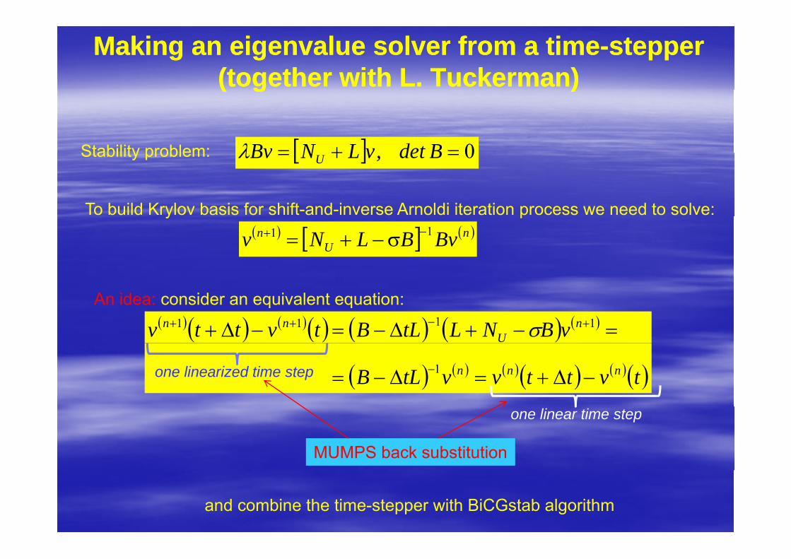
Making an eigenvalue solver from a timeMaking an eigenvalue solver from a time--stepper stepper ((together with Ltogether with L. Tuckerman). Tuckerman)(( gg ))

Stability problem: 0 BdetvLNBvStability problem: 0 Bdet,vLNBv U

To build Krylov basis for shift-and-inverse Arnoldi iteration process we need to solve:y p n

Un BvBLNv 11

vBNLtLBtvttv nU

nn 1111 An idea: consider an equivalent equation:

tvttvvtLB nnn 1one linearized time step

one linear time step

MUMPS back substitution

and combine the time-stepper with BiCGstab algorithm

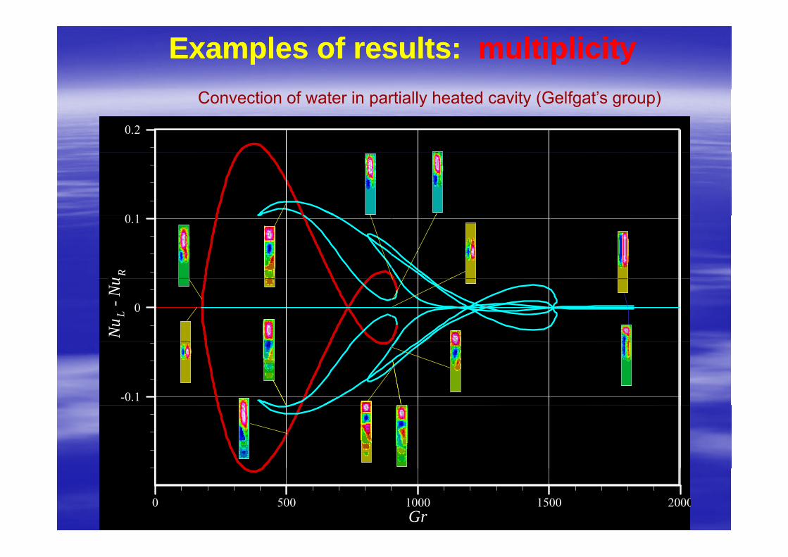
Examples of results:Examples of results: multiplicitymultiplicity

0.2

Convection of water in partially heated cavity (Gelfgat’s group)

0 1

u

0.1

RN

u-N

u

0L

-0.1

Gr0 500 1000 1500 2000

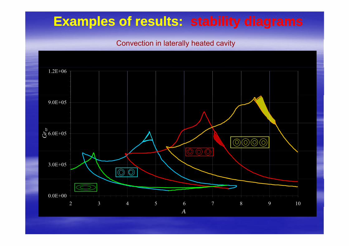
Examples of results:Examples of results: stability diagramsstability diagramsConvection in laterally heated cavity

1.2E+06

9.0E+05

6.0E+05Gr c

r

3.0E+05

0.0E+002 3 4 5 6 7 8 9 10

A

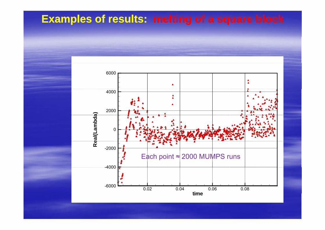
Examples of results:Examples of results: melting of a square blockmelting of a square block

T=06000

a)

2000

4000

T=0T=Tmelting

eal(L

ambd

a

0

Re

-4000

-2000

Each point ≈ 2000 MUMPS runs

T=0time

0.02 0.04 0.06 0.08-6000

-4000

time

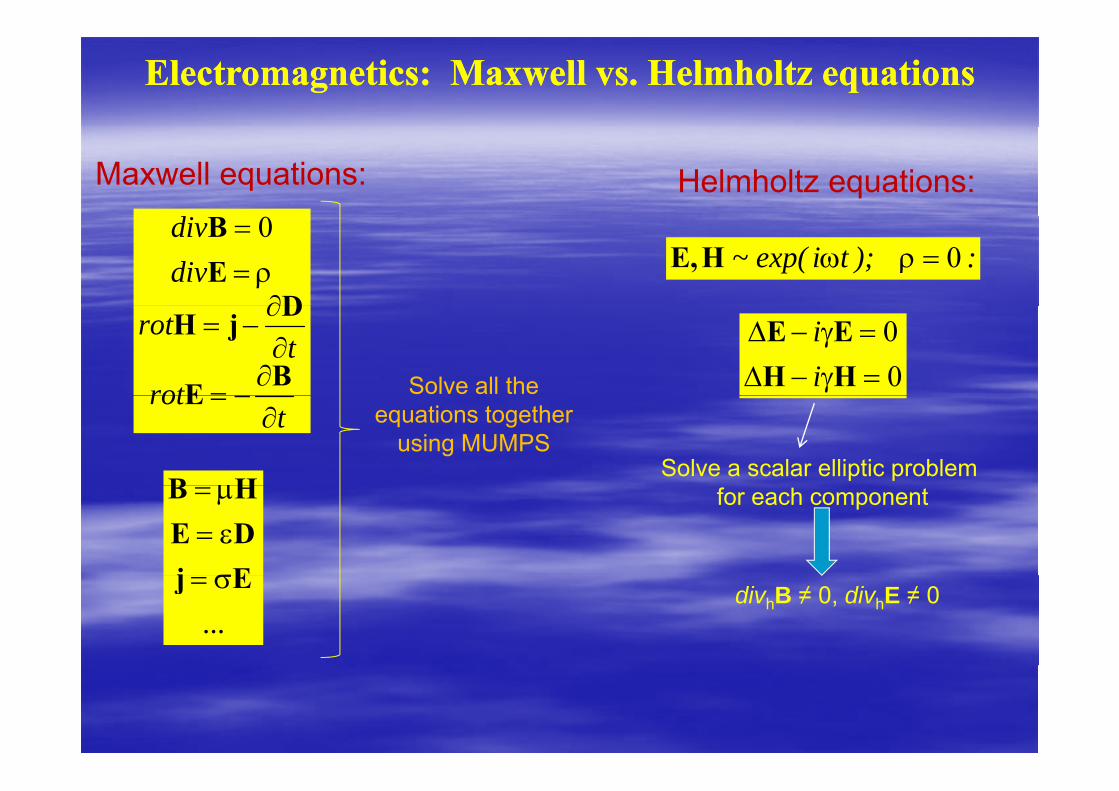
ElectromagneticsElectromagnetics: Maxwell vs. Helmholtz equations: Maxwell vs. Helmholtz equations

Maxwell equations: Helmholtz equations:ddivdiv

DEB 0

:);tiexp(~ 0HE,

rott

rot

BE

DjH

00

HHEE

ii

Solve all the t

rot

E

HB Solve a scalar elliptic problem

equations together using MUMPS

EjDEHB

for each component

...Ej divhB ≠ 0, divhE ≠ 0

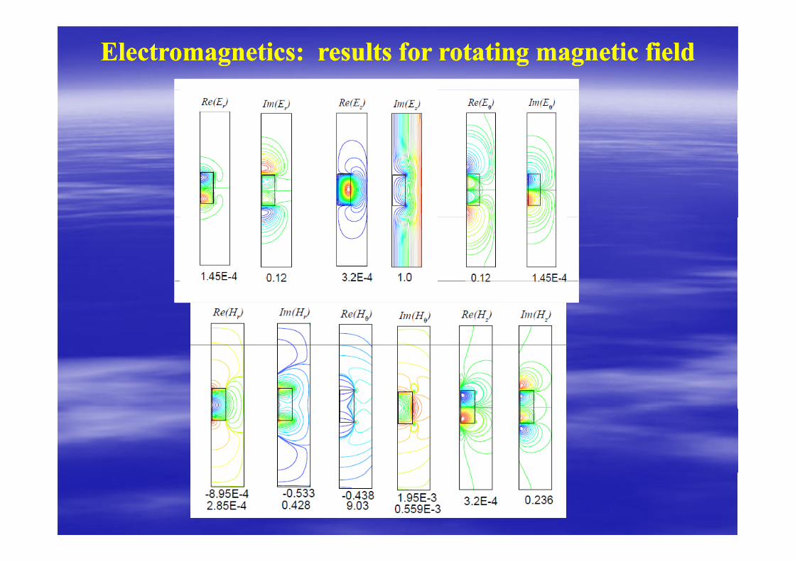
ElectromagneticsElectromagnetics: results for rotating magnetic field: results for rotating magnetic field

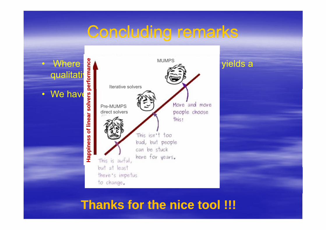
ConcludingConcluding remarksremarksConcluding Concluding remarksremarks

• Where MUMPS is successfully applies it yields acece MUMPS • Where MUMPS is successfully applies it yields a qualitative improvement of results

perf

orm

anc

perf

orm

anc

Iterative solvers

• We have more ideas for future studiesar

sol

vers

par

sol

vers

p

Pre-MUMPS direct solvers

ss o

f lin

eass

of l

inea

Hap

pine

Hap

pine

Thanks for the nice tool !!!Thanks for the nice tool !!!