Solving of linear Equations using SVD

nSolving a linear equationnGauss elimination and SVDnHowTonSome tricks for SVD Jochen Schieck

MPI Munich

Problems in Linear Equations

n generally in solving Ax=b two error contributions possible:

1. intrinsic errors in A and b2. numerical errors due to rounding

Mathematical description and handling available

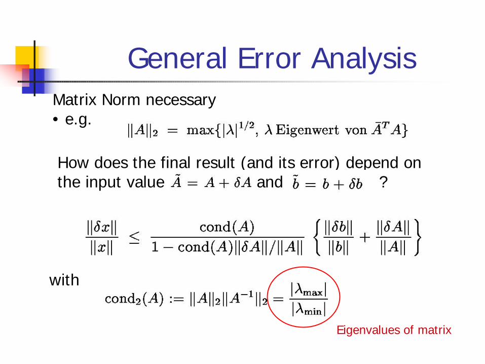
How does the final result (and its error) depend on the input value and ?

General Error AnalysisMatrix Norm necessary• e.g.

with

Eigenvalues of matrix

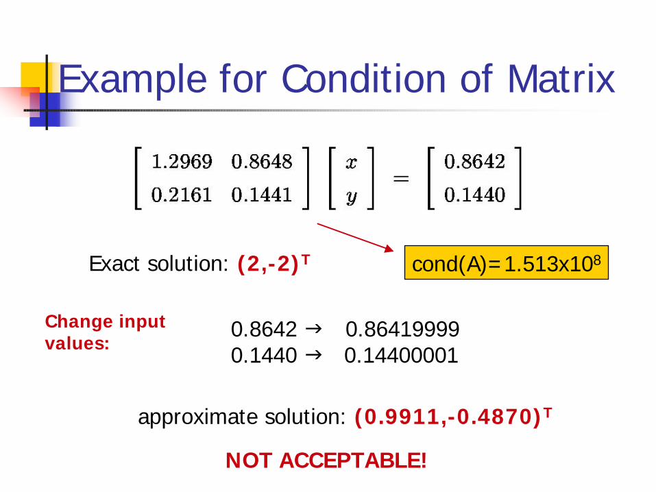
Example for Condition of Matrix

Exact solution: (2,-2)T

0.8642 g 0.864199990.1440 g 0.14400001

Change input values:

approximate solution: (0.9911,-0.4870)T

NOT ACCEPTABLE!

cond(A)=1.513x108

Gauss Elimination

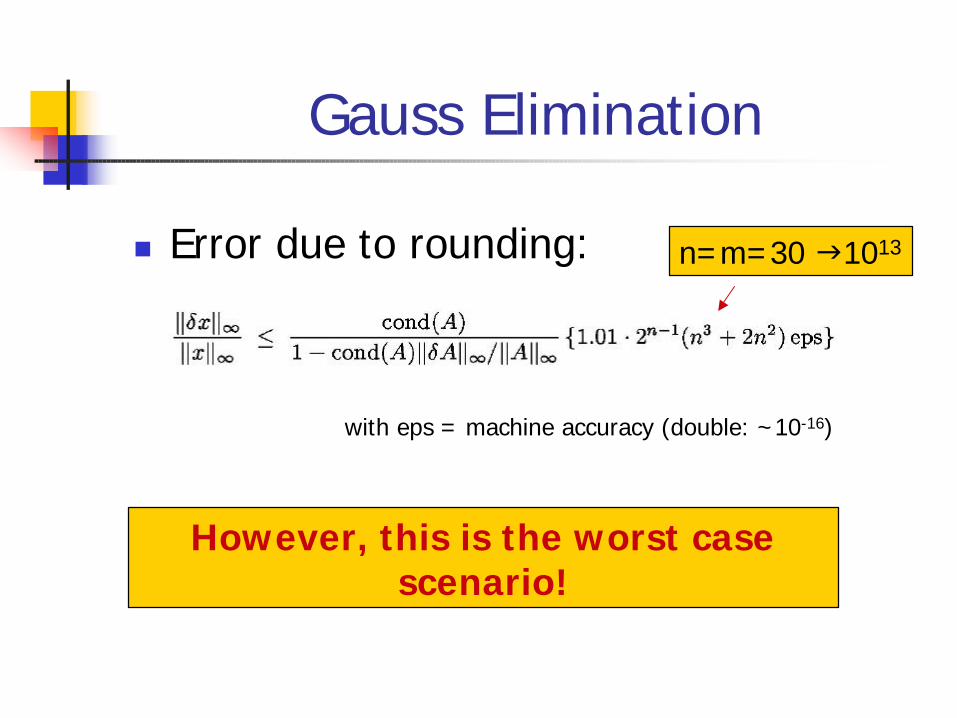
n Error due to rounding:

with eps = machine accuracy (double: ~10-16)

However, this is the worst case scenario!

n=m=30 g1013

Singular Value Decomposition

n here for (nxn) case, valid also for (nxm)n Solution of linear equations numerically

difficult for matrices with bad condition:Ø regular matrices in numeric approximation

can be singularØ SVD helps finding and dealing with the

sigular values

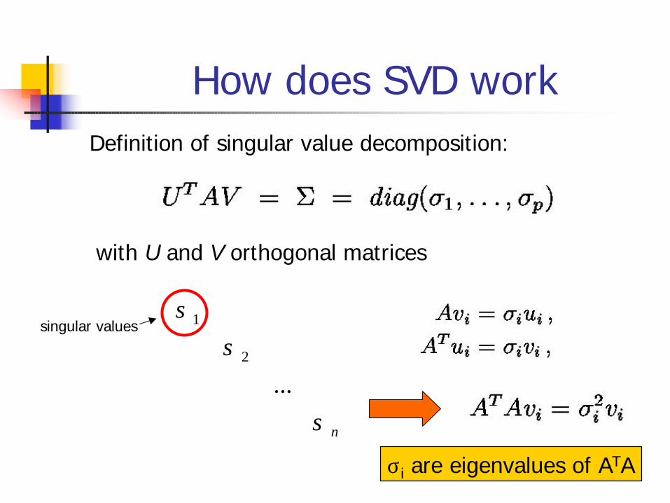
How does SVD workDefinition of singular value decomposition:

with U and V orthogonal matrices

nσ

σσ

...2

1singular values

σi are eigenvalues of ATA

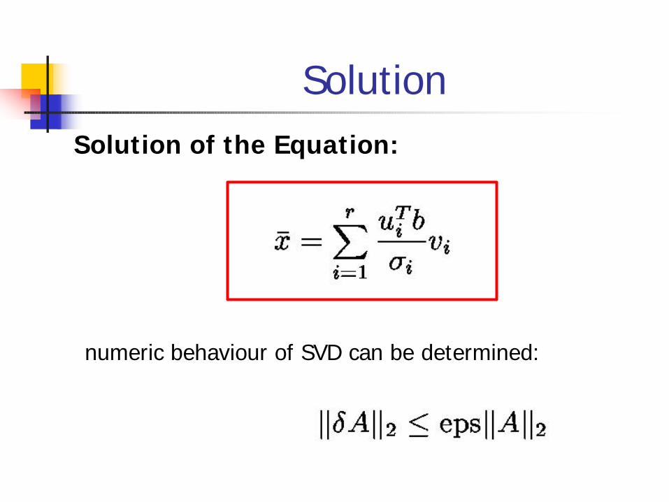
SolutionSolution of the Equation:

numeric behaviour of SVD can be determined:

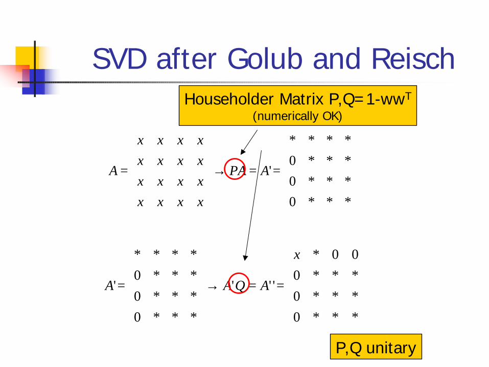
SVD after Golub and Reisch

==→

=

***0***0***0****

'APA

xxxxxxxxxxxxxxxx

A

==→

=

***0***0***000*

'''

***0***0***0****

'

x

AQAA

Householder Matrix P,Q=1-wwT

(numerically OK)

P,Q unitary

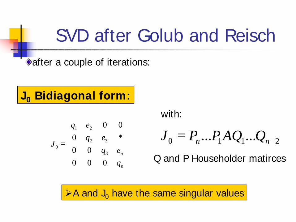
SVD after Golub and Reisch

=

n

n

qeq

eqeq

J

00000

*000

3

32

21

0

after a couple of iterations:

2110 ...... −= nn QAQPPJ

with:

Q and P Householder matirces

ØA and J0 have the same singular values

J0 Bidiagonal form:

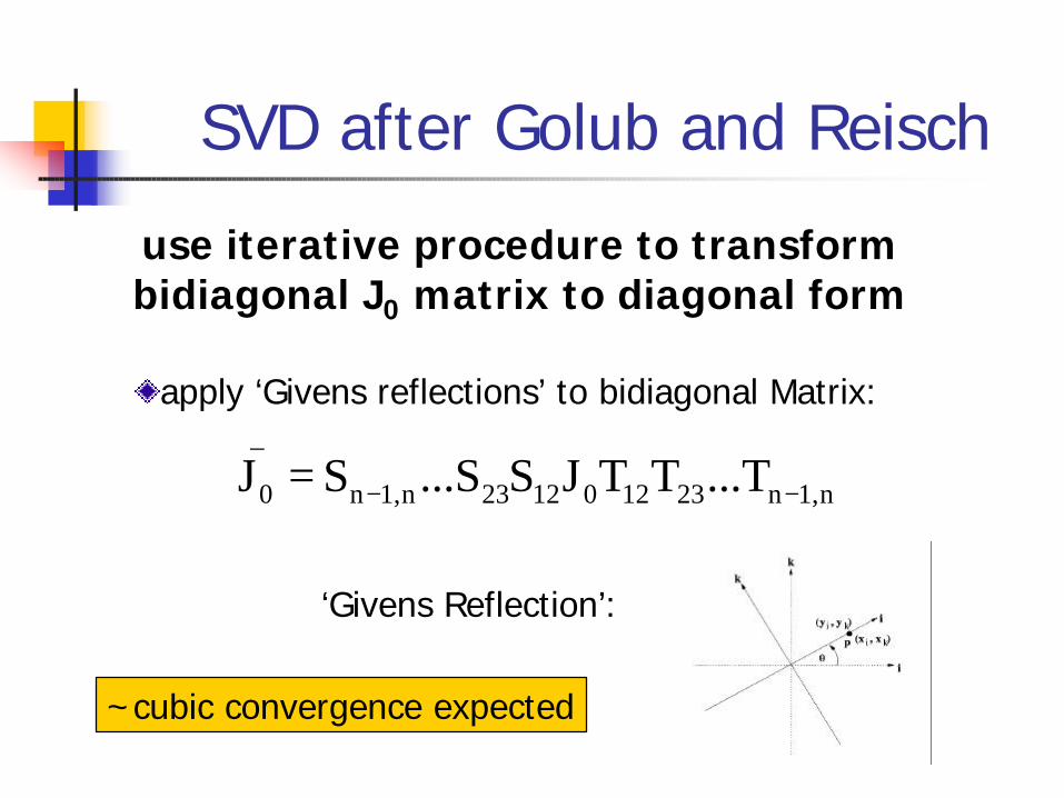
SVD after Golub and Reisch

apply ‘Givens reflections’ to bidiagonal Matrix:

use iterative procedure to transform bidiagonal J0 matrix to diagonal form

n1,n231201223n1,n

_

0 ...TTTJS...SSJ −−=

‘Givens Reflection’:

~cubic convergence expected

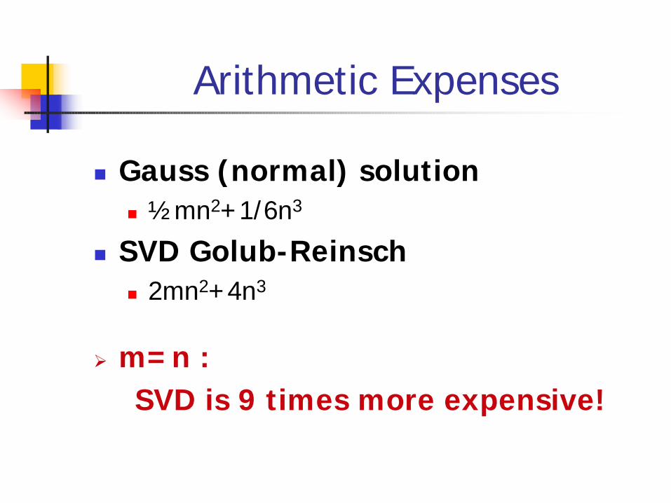
Arithmetic Expenses

n Gauss (normal) solutionn ½mn2+1/6n3

n SVD Golub-Reinschn 2mn2+4n3

Ø m=n :SVD is 9 times more expensive!

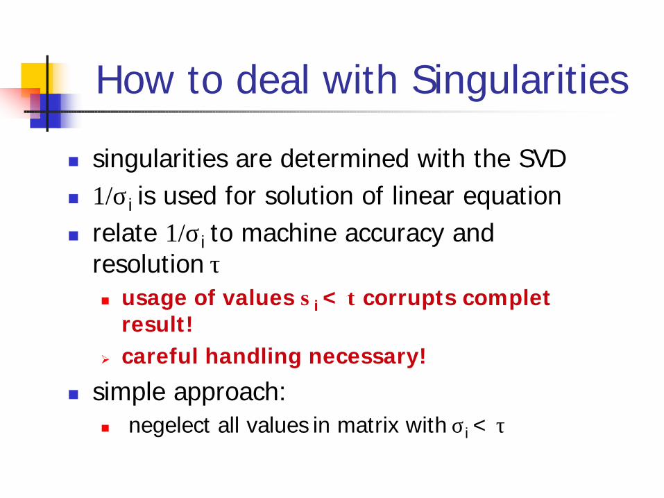
How to deal with Singularities

n singularities are determined with the SVD n 1/σi is used for solution of linear equation n relate 1/σi to machine accuracy and

resolution τn usage of values σi < τ corrupts complet

result!Ø careful handling necessary!

n simple approach:n negelect all values in matrix with σi < τ

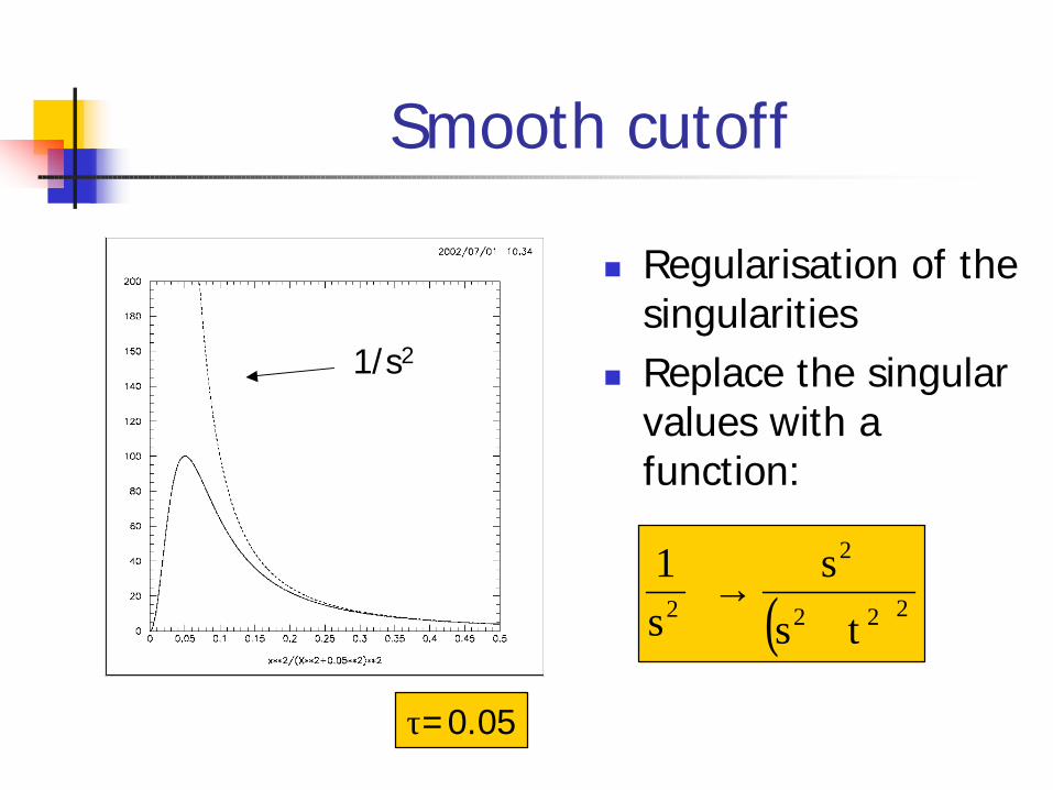
Smooth cutoff

n Regularisation of the singularities

n Replace the singular values with a function:

( )222

2

2ts

ss1

+→

τ=0.05

1/s2

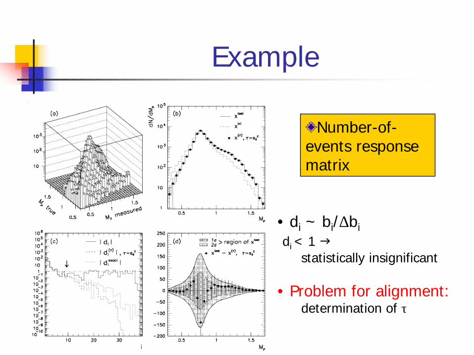
Example

Number-of-events response matrix

• di ~ bi/∆bi di < 1 g

statistically insignificant

• Problem for alignment:determination of τ

Conclusion

n Numeric Solution of a regular linear equation can be distorted by singular behaviour

n SVD returns singular valuesn Singular values can be handeld with

smooth cut off n Mathemaical well described procedure