solving fluid dynamics problems with matlab · pdf filematlab allows us to use a powerful...

12

Solving Fluid Dynamics Problems with Matlab

Rui M. S. Pereira1 and Jitesh S. B. Gajjar2

1 Centre of Mathematics, University of Minho2School of Mathematics, University of Manchester

1Portugal2United Kingdom

1. Introduction

MATLAB (short for Matrix Laboratory) was created by Cleve Moler and Jack Little in theseventies. It is a programming language for technical computing. Its environment is easyto work with, the syntax is very simple and intuitive, it has powerful toolboxes to treatmany different problems in engineering, and it allows us to produce fantastic graphics as theprogramme runs. It also allows us to create a graphical interface (via graphical user interfaces- GUIs) that gives our programme a look that is very close to professional software.Because of many of the mentioned features, a MATLAB code can be very compact, allowinganyone to have "the big picture" of any code without have to look at all its details. Anothergreat advantage of Matlab is that, if the code is written in a vectorized form, the code canrun much faster than if it was written in the traditional form (’a la C/fortran’). The fact thatMATLAB allows us to use a powerful toolbox for sparse matrices, is also a great advantagesince, many traditional linear algebra operations can be highly improved, allowing the codesto run much faster than it would run with the traditional linear algebra functions.In our work we have made extensive use of MATLAB to do ’proof of concept’ studies,especially when developing new algorithms and techniques for solving systems of couplednonlinear partial differential equations, such as those which arise in fluid dynamics. Thisincludes, for instance, codes for investigating instabilities in lid-driven cavities, Boppana andGajjar (2010a), instabilities in flow past circular cylinders, Boppana and Gajjar (2010b), andtransonic flow past aerofoils Pereira and Gajjar (2010). In some cases MATLAB is used in itsown right for solving small problems, but the fact that MATLAB is an interpreted languagemeans that for increasing problem sizes, the MATLAB version of the code can be much slowerthan equivalent versions in other languages especially when one is dealing with very largesparse matrices. On the other hand the beauty of MATLAB is that much of the hard workis buried in the simple syntax and hidden from the user. An example of this is the use ofthe backslash operator for solving linear systems. Whether the system is sparse or full, themanner in which the equations are solved is hidden from the user and this greatly facilitatescode development. In the equivalent fortran versions of the code the replacement for the ’\’operation requires considerable work and the code translation process is no longer a trivialexercise.In this chapter we will discuss the use of hybrid spectral methods to solve two andthree-dimensional problems using MATLAB. There is an excellent book by Trefethen (2000)which discusses the application of spectral methods using MATLAB to solve ordinary and

2 Engineering Education and Research Using MATLAB

partial differential equations, and which provides the foundation for the techniques describedbelow.To motivate the ideas we first consider the solution of a model equation of the form

a(x, y)ψxx + b(x, y)ψyy + c(x, y)ψx + e(x, y)ψy + f (x, y)ψ = g(x, y),

say with Dirichlet boundary conditions in a rectangular domain. To obtain a numericalsolution to this problem the first step is to choose an appropriate method and discretization.In our work we have used a combination of spectral methods in one or two dimensions andhigh order finite difference methods in another dimension. The main reasons for this choiceare that a hybrid approach combines the accuracy of spectral methods together with flexibilityin comparison to using spectral methods on their own. One restriction with the use of spectralmethods is that one needs to use somewhat simplified geometries. A hybrid approach givesmore flexibility in this respect. Another important reason stems from consideration of thetype of matrix patterns which arise. With finite differences in say the x direction and spectralcollocation in the y direction, the coefficient matrix with the unknowns ordered in terms ofincreasing y values for a fixed x value, has a particular sparsity pattern dependent on the orderof the finite-differencing used. Second order finite-differencing leads to a a block tridiagonalmatrix whilst with fourth-order finite differences, the matrix is block-pentadiagonal of theform:

AqΨq−2 + BqΨq−1 + CqΨq + DqΨq+1 + EqΨq+2 = Rq, q = 0, 1, ..., M. (1)

Here Ψq is the vector of unknowns at location x = xq, M + 1 is typically the number of pointsin the x direction and the block matrices are of size N + 1 by N + 1 where N + 1 spectral pointsare used.Using MATLAB it is not too difficult to generate a short code to solve the above discrete systemand the book by Trefethen (2000) gives plenty of such examples. The problem becomes morechallenging when N and M become large, as for example in some fluid flow applicationswhere large N, M values are needed to resolve regions of the flow where the solution changesvery rapidly. When using a large number of points the sparse matrix facilities of MATLABcome into their own. The whole coefficient matrix does not need to be stored and by declaringthis as a sparse matrix, only the non-zero entries of the block matrices are calculated. Thisavoids having to store a very large and sparse matrix which can quickly lead to memoryproblems.Increasing the order of the scheme leads to increased bandwidths. This sparsity pattern canbe exploited for 2nd, 4th or even 6th finite-differencing with a direct solver. However, withspectral methods in two directions, unless the differential operator involved has a specialform, it is not immediately possible to utilize the sparse nature of the matrix. Whilst thisdoes not pose any intrinsic difficulties if one is coding in MATLAB, with increased number ofpoints the solution phase can become very memory intensive and requires a lot of processortime. The use of the hybrid approach in our work is motivated in part by the observation thatthe sparse matrix structure can be exploited to write efficient solvers, which not only workwell with MATLAB, but can be coded directly in other languages. MATLAB provides for anexcellent environment in which one can test and develop solvers of this type.The above techniques have been successfully applied to investigate a whole range of differentflow problems governed by the Navier-Stokes and related equations. In the first example weconsider the onset of instability in the lid-driven cavity flow. MATLAB was used to generateresults on coarse grids and do preliminary eigenvalue computations. For very fine grids, the

Solving Fluid Dynamics Problems with Matlab 3

computations were performed in Fortran 95. The problem is described in detail in Boppanaand Gajjar (2010a).The second problem concerns the onset of instability in the flow past a row of circularcylinders. Again the same technqiues have been used but for a more complicated geometry.This problem is described in detail in Boppana and Gajjar (2010b).The third problem we discuss concerns the inviscid transonic flows past thin airfoils. Herethe governing equations are nonlinear and of mixed type and the flow can contain shockwave discontinuities for certain parameter values. The full details are given in Pereira andGajjar (2010). The same methods as described above are used except now type differencingneeds to be incorporated to allow for the different flow behaviours in regions of subsonicand supersonic flow. The method is fast and very robust and we are able to compute steadyflows with strong shocks. The code was written in MATLAB, using vectorization whenpossible, and, in order to produce a good interface with the user, we used GUIs (graphicaluser interfaces) from MATLAB. The result was a fast and accurate code, with the extra bonusof a very good interface with the user, without a lot of effort in terms of programming. The factthat graphical results can be shown immediately, saves us a lot of work, both on the analysisof the results and on its presentation.

2. Instabilities in lid-driven cavities.

To motivate the techniques used in our work we first consider a model elliptic equation of theform

a(x, y)ψxx + b(x, y)ψyy + c(x, y)ψx + e(x, y)ψy + f (x, y)ψ = g(x, y) (2)

with say Dirichlet boundary conditions in a square domain 0 ≤ x, y ≤ 1. It is assumed thatthe functions a, b, c, e, f , g are smooth functions of x and y.The discrete solution to the equations will be obtained at a set of grid points on an (M +1) × (N + 1) grid say with the nodes, x = xj, j = 0, . . . , M with x1 = 0, xM = 1, andy = yk, 0 ≤ k ≤ N with y0 = 1, yN = 1, and at these points we set ψj,k = ψ(xj, yk).We will assume that derivatives in the x− and y− directions may be approximated as

∂ψ

∂x(xj, yk) =

M

∑q=0

(Dx)j,qψq,k,∂2ψ

∂x2 (xj, yk) =M

∑q=0

(Dxx)j,qψq,k,

∂ψ

∂y(xj, yk) =

M

∑q=0

(Dy)k,qψj,q,∂2ψ

∂y2 (xj, yk) =M

∑q=0

(Dyy)k,qψj,q. (3)

Given the type and order of discretisation, the elements of the matrices Dx, Dxx, Dy, Dyy areknown. For example with second-order central finite differences, at an interior point of auniform grid in x with ∆x = xj − xj−1, we have

(Dx)j,j−1 = − 12∆x

, (Dx)j,j+1 =1

2∆x,

(Dxx)j,j−1 =1

∆2x

, (Dxx)j,j+1 =1

∆2x

, (Dxx)j,j = − 2∆2

x, 1 ≤ j ≤ M− 1,

and zero otherwise. If we take Chebychev collocation in the y−direction, the Dy, Dyy arethe Chebychev differentiation matrices and are given in a number of places, see for example


Weideman and Reddy (2003) or Trefethen (2000), where MATLAB code to generate thematrices is given.Discretization of the equation 2 leads to the set of equations

aj,k

M

∑q=0

(Dxx)j,qψq,k + bj,k

M

∑q=0

(Dyy)k,qψj,q + cj,k

M

∑q=0

(Dx)j,qψq,k + ej,k

M

∑q=0

(Dy)k,qψj,q + f j,kψj,k = gj,k,

(4)at the interior points 1 ≤ j ≤ M− 1, 1 ≤ k ≤ N − 1. At the boundaries we have ψ = 0.The discrete set (4) can be combined into a compact form as

[DIAG(a)(IN+1 ⊕Dxx) + DIAG(c)(IN+1 ⊕Dx)] Ψ+[DIAG(b)(Dyy ⊕ IM+1) + DIAG(e)(Dy ⊕ IM+1)

]Ψ + DIAG(f)Ψ = g , (5)

where Ψ denotes the vector of unknowns, A ⊕ B is the kronecker tensor product of twomatrices A, B (which in MATLAB is represented by the kron(A,B) operator), and DIAG(v)is as in MATLAB the diagonal matrix with entries given by the vector v, and IM+1 is theidentity matrix of order M + 1. Certain rows of the matrix operator in (5) are also modifiedwhen the boundary conditions are incorporated.The linear sytem may be represented as

SΨ = R. (6)

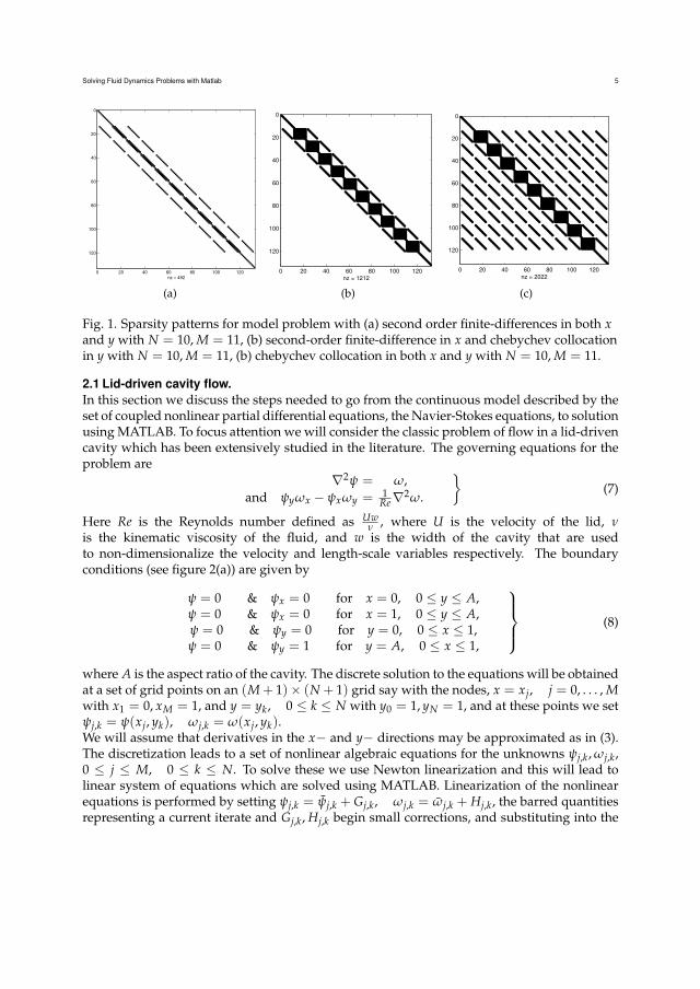
Once the coefficient matrix S and the right hand sides have been computed, the solution justinvolves the use of the \ operator with Ψ = S\R. From the user perspective other thandeclaring that the matrices involved are sparse matrices, no additional special treatment isrequired to obtain the solution of the linear systems.Given the discretization matrices, the above system is easy to code in MATLAB. For certaindiscretizations however, the linear systems outlined above can be huge and highly sparse.The bandwidth of the coefficient matrix increases with increasing order of differences used,and with spectral methods in two directions, the coefficient matrix has the sparsity patternsimilar to that in figure 1(c), obtained using the spy function in MATLAB. On the other handby taking second-order finite differences in the x−direction and spectral collocation in they−direction, with a particular ordering of grid points, the matrices can be written in blocktridiagonal form as shown in figure 1(a),1(b), or with fourth order finite-differencing in x thelinear system is block pentadiagonal. With 2nd, 4th or even 6th finite-differencing the linearsystems can be solved with a direct solver but with spectral methods in two directions, unlessthe differential operator involved has a special form, it is not immediately possible to utilizethe sparse nature of the matrix. Whilst this does not pose any intrinsic difficulties if one iscoding in MATLAB, with increased number of points the solution phase can become verymemory intensive and requires a lot of processor time. The use of the hybrid approach in ourwork is motivated in part by the observation that the sparse matrix structure can be exploitedto write efficient solvers, which not only work well with MATLAB, but can be coded directlyin other languages. MATLAB provides for an excellent environment in which one can test anddevelop solvers of this type. In our work we have written our own direct block solvers as wellas making direct use of the \ operator with a sparse matrix.In the MATLAB codes when constructing the coefficient matrices, we use the functions speyeor spalloc for initially creating the sparse matrices. After this only the non-zero elements ofthe matrices are assigned.


0 20 40 60 80 100 120

0

20

40

60

80

100

120

nz = 492

(a)

0 20 40 60 80 100 120

0

20

40

60

80

100

120

nz = 1212

(b)

0 20 40 60 80 100 120

0

20

40

60

80

100

120

nz = 2022

(c)

Fig. 1. Sparsity patterns for model problem with (a) second order finite-differences in both xand y with N = 10, M = 11, (b) second-order finite-difference in x and chebychev collocationin y with N = 10, M = 11, (b) chebychev collocation in both x and y with N = 10, M = 11.

2.1 Lid-driven cavity flow.In this section we discuss the steps needed to go from the continuous model described by theset of coupled nonlinear partial differential equations, the Navier-Stokes equations, to solutionusing MATLAB. To focus attention we will consider the classic problem of flow in a lid-drivencavity which has been extensively studied in the literature. The governing equations for theproblem are

∇2ψ = ω,and ψyωx − ψxωy = 1

Re∇2ω.

(7)

Here Re is the Reynolds number defined as Uwν , where U is the velocity of the lid, ν

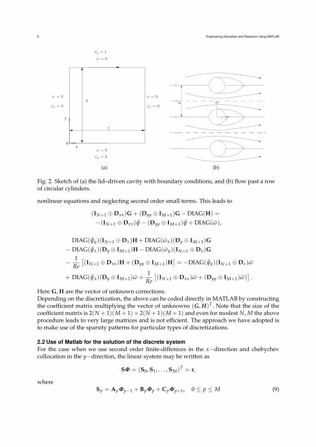
is the kinematic viscosity of the fluid, and w is the width of the cavity that are usedto non-dimensionalize the velocity and length-scale variables respectively. The boundaryconditions (see figure 2(a)) are given by

ψ = 0 & ψx = 0 for x = 0, 0 ≤ y ≤ A,ψ = 0 & ψx = 0 for x = 1, 0 ≤ y ≤ A,ψ = 0 & ψy = 0 for y = 0, 0 ≤ x ≤ 1,ψ = 0 & ψy = 1 for y = A, 0 ≤ x ≤ 1,

(8)

where A is the aspect ratio of the cavity. The discrete solution to the equations will be obtainedat a set of grid points on an (M + 1)× (N + 1) grid say with the nodes, x = xj, j = 0, . . . , Mwith x1 = 0, xM = 1, and y = yk, 0 ≤ k ≤ N with y0 = 1, yN = 1, and at these points we setψj,k = ψ(xj, yk), ωj,k = ω(xj, yk).We will assume that derivatives in the x− and y− directions may be approximated as in (3).The discretization leads to a set of nonlinear algebraic equations for the unknowns ψj,k, ωj,k,0 ≤ j ≤ M, 0 ≤ k ≤ N. To solve these we use Newton linearization and this will lead tolinear system of equations which are solved using MATLAB. Linearization of the nonlinearequations is performed by setting ψj,k = ψj,k + Gj,k, ωj,k = ωj,k + Hj,k, the barred quantitiesrepresenting a current iterate and Gj,k, Hj,k begin small corrections, and substituting into the


0x

y

A

1

ψ = 0ψ = 0

ψ = 0

ψ = 0

ψx = 0ψx = 0

ψy = 0

ψy = 1

(a)

W

x

y

1

(b)

Fig. 2. Sketch of (a) the lid–driven cavity with boundary conditions, and (b) flow past a rowof circular cylinders.

nonlinear equations and neglecting second order small terms. This leads to

(IN+1 ⊕Dxx)G + (Dyy ⊕ IM+1)G−DIAG(H) =−(IN+1 ⊕Dxx)ψ− (Dyy ⊕ IM+1)ψ + DIAG(ω),

DIAG(ψy)(IN+1 ⊕Dx)H + DIAG(ωx)(Dy ⊕ IM+1)G

− DIAG(ψx)(Dy ⊕ IM+1)H−DIAG(ωy)(IN+1 ⊕Dx)G

− 1Re[(IN+1 ⊕Dxx)H + (Dyy ⊕ IM+1)H

]= −DIAG(ψy)(IN+1 ⊕Dx)ω

+ DIAG(ψx)(Dy ⊕ IM+1)ω +1

Re[(IN+1 ⊕Dxx)ω + (Dyy ⊕ IM+1)ω)

].

Here G, H are the vector of unknown corrections.Depending on the discretization, the above can be coded directly in MATLAB by constructingthe coefficient matrix multiplying the vector of unknowns (G, H)T . Note that the size of thecoefficient matrix is 2(N + 1)(M + 1)× 2(N + 1)(M + 1) and even for modest N, M the aboveprocedure leads to very large matrices and is not efficient. The approach we have adopted isto make use of the sparsity patterns for particular types of discretizations.

2.2 Use of Matlab for the solution of the discrete systemFor the case when we use second order finite-differeces in the x−direction and chebychevcollocation in the y−direction, the linear system may be written as

SΦ = (S0, S1, . . . , SM)T = r,

whereSp = ApΦp−1 + BpΦp + CpΦp+1, 0 ≤ p ≤ M (9)


Φp = (Gp0, Gp1, . . . , GpN , Hp0, Hp1, . . . HpN)T , Φ = (Φ0, Φ1, . . . , ΦM)T ,

with A0 = CM = 0. This represents a particular ordering of unknowns and gives rise to theblock tridiagonal system in (9). With 4th order finite-differencing in x the linear system isblock pentadiagonal.The coefficient matrices Ap, BP, Cp can be extracted from the discrete equations above and

Ap =

( 1∆2

xIN+1 O

12∆x

DIAG(Dyωp) − 12∆x

DIAG(Up)− 1Re∆2

xIN+1

),

Bp =

Dyy − 2∆2

xIN+1 −IN+1

DIAG(Ωx p)Dy DIAG(Vp)Dy + 1Re

[2

∆2xIN+1 −Dyy

] ,

Cp =

( 1∆2

xIN+1 O

12∆x

DIAG(Dyωp) 12∆x

DIAG(Up)− 1Re∆2

xIN+1

),

with

Up = Dyψp, Ωx p =ωp+1 − ωp−1

2∆x, Vp = − ψp+1 − ψp−1

2∆x.

The above excludes the boundary conditions, but these just alter certain rows of the matrices.In MATLAB the individual entries of the block matrices are easily computed and the S matrixis updated via

S(1 + 2p(N + 1) : 2(p + 1)(N + 1), 1 + 2(p− 1)(N + 1) : 2p(N + 1)) = Ap,

S(1 + 2p(N + 1) : 2(p + 1)(N + 1), 1 + 2p(N + 1) : 2(p + 1)(N + 1)) = Bp,

S(1 + 2p(N + 1) : 2(p + 1)(N + 1), 1 + 2(p + 1)(N + 1) : 2(p + 2)(N + 1)) = CP,

for 1 ≤ p ≤ M− 1.

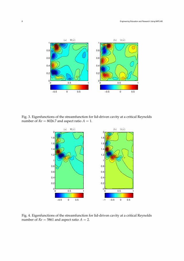
2.3 Results for lid-driven cavityThe method described above was used to compute the flow in a lid-driven cavity. Thesame techniques used were adapted to firstly compute the steady flow, and then investigatethe instability of the flow via simulations as well as solving the linear eigenvalue problemassuming normal mode disturbances proportional to eλt. Further details of the techniquesmay be found in Boppana and Gajjar (2010a). MATLAB was also used in the eigenvalueanalysis. In fact the eigenvalue problem required to be solved takes the form

SΦ = λT,

which is a generalised eigenvalue problem. The matrix S is the same as the Jacobian matrixof the linear system after Newton linearization, and T is a singular diagonal matrix. Theeigenvalue problem is solved in MATLAB using the eig function. In other related problemsthe routine sptarn available in the PDE toolbox was used for the solution of the generalisedeigenvalue problem.In figure 3 we have shown the real and imaginary parts of eigenfunctions for the disturbancestreamfunction ψ for aspect ratios of A = 1 and A = 2 at the onset of instability, obtainedfrom a solution of the eigenvalue problem. The advantage of working with MATLAB is thatsuch plots can be generated at the same time as the computation is in progress.More extensive results and details are documented in Boppana and Gajjar (2010a).


(a) ℜ(ψ)

0 0.5 10

0.2

0.4

0.6

0.8

1

−0.5 0 0.5

(b) ℑ(ψ)

0 0.5 10

0.2

0.4

0.6

0.8

1

−0.5 0 0.5

Fig. 3. Eigenfunctions of the streamfunction for lid-driven cavity at a critical Reynoldsnumber of Re = 8026.7 and aspect ratio A = 1.

(a) ℜ(ψ)

0 0.5 10

0.2

0.4

0.6

0.8

1

1.2

1.4

1.6

1.8

2

−0.5 0 0.5

(b) ℑ(ψ)

0 0.5 10

0.2

0.4

0.6

0.8

1

1.2

1.4

1.6

1.8

2

−1 −0.5 0 0.5

Fig. 4. Eigenfunctions of the streamfunction for lid-driven cavity at a critical Reynoldsnumber of Re = 5861 and aspect ratio A = 2.


3. Flow past circular cylinders

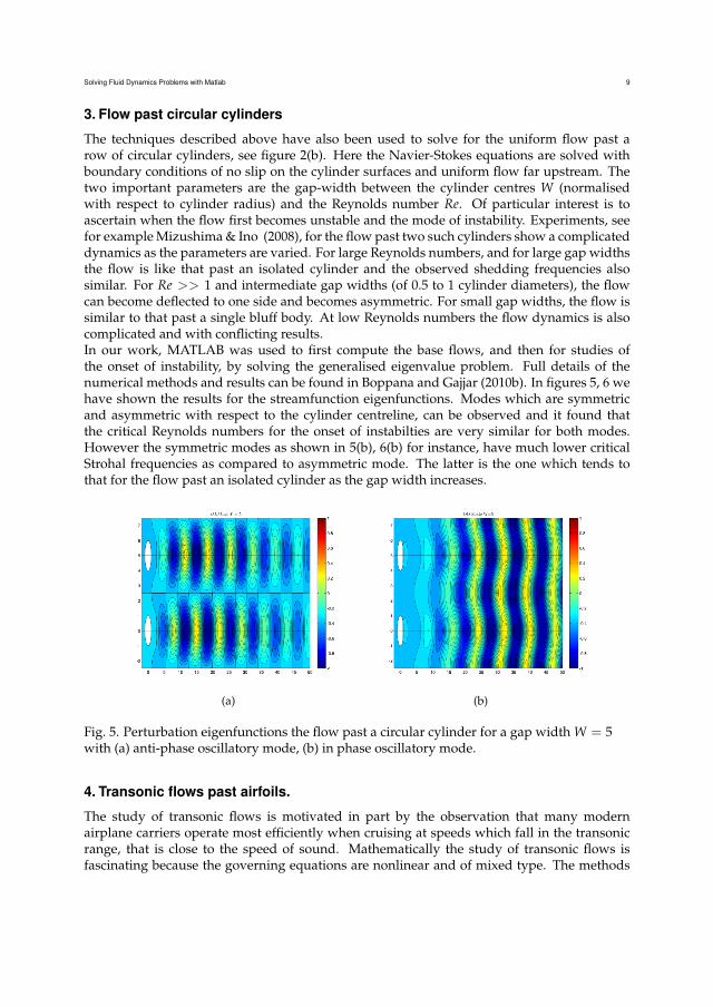
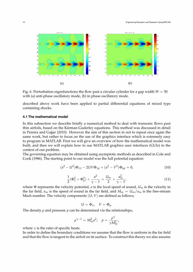
The techniques described above have also been used to solve for the uniform flow past arow of circular cylinders, see figure 2(b). Here the Navier-Stokes equations are solved withboundary conditions of no slip on the cylinder surfaces and uniform flow far upstream. Thetwo important parameters are the gap-width between the cylinder centres W (normalisedwith respect to cylinder radius) and the Reynolds number Re. Of particular interest is toascertain when the flow first becomes unstable and the mode of instability. Experiments, seefor example Mizushima & Ino (2008), for the flow past two such cylinders show a complicateddynamics as the parameters are varied. For large Reynolds numbers, and for large gap widthsthe flow is like that past an isolated cylinder and the observed shedding frequencies alsosimilar. For Re >> 1 and intermediate gap widths (of 0.5 to 1 cylinder diameters), the flowcan become deflected to one side and becomes asymmetric. For small gap widths, the flow issimilar to that past a single bluff body. At low Reynolds numbers the flow dynamics is alsocomplicated and with conflicting results.In our work, MATLAB was used to first compute the base flows, and then for studies ofthe onset of instability, by solving the generalised eigenvalue problem. Full details of thenumerical methods and results can be found in Boppana and Gajjar (2010b). In figures 5, 6 wehave shown the results for the streamfunction eigenfunctions. Modes which are symmetricand asymmetric with respect to the cylinder centreline, can be observed and it found thatthe critical Reynolds numbers for the onset of instabilties are very similar for both modes.However the symmetric modes as shown in 5(b), 6(b) for instance, have much lower criticalStrohal frequencies as compared to asymmetric mode. The latter is the one which tends tothat for the flow past an isolated cylinder as the gap width increases.

(a) (b)

Fig. 5. Perturbation eigenfunctions the flow past a circular cylinder for a gap width W = 5with (a) anti-phase oscillatory mode, (b) in phase oscillatory mode.

4. Transonic flows past airfoils.

The study of transonic flows is motivated in part by the observation that many modernairplane carriers operate most efficiently when cruising at speeds which fall in the transonicrange, that is close to the speed of sound. Mathematically the study of transonic flows isfascinating because the governing equations are nonlinear and of mixed type. The methods


(a) (b)

Fig. 6. Perturbation eigenfunctions the flow past a circular cylinder for a gap width W = 50with (a) anti-phase oscillatory mode, (b) in phase oscillatory mode.

described above work have been applied to partial differential equations of mixed typecontaining shocks.

4.1 The mathematical model

In this subsection we describe briefly a numerical method to deal with transonic flows pastthin airfoils, based on the Kárman-Guderley equations. This method was discussed in detailin Pereira and Gajjar (2010). However the aim of this section in not to repeat once again thesame work, but rather to focus on the use of the graphics interface which is extremely easyto program in MATLAB. First we will give an overview of how the mathematical model wasbuilt, and then we will explain how to use MATLAB graphics user interfaces (GUIs) in thecontext of our problem.The governing equation may be obtained using asymptotic methods as described in Cole andCook (1986). The starting point to our model was the full potential equation:

(a2 −U2)Φxx − 2UVΦxy + (a2 −V2)Φyy = 0, (10)

12(Φ2

x + Φ2y) +

a2

γ− 1=

U∞

2+

a2∞

γ− 1, (11)

where Φ represents the velocity potential, a is the local speed of sound, U∞ is the velocity inthe far field, a∞ is the speed of sound in the far field, and M∞ = U∞/a∞ is the free-streamMach number. The velocity components (U, V) are defined as follows,

U = Φx, V = Φy.

The density ρ and pressure p can be determined via the relationships,

ργ−1 = M2∞a2; p =

ργ

γM2∞

,

where γ is the ratio of specific heats.In order to define the boundary conditions we assume that the flow is uniform in the far fieldand that the flow is tangent to the airfoil on its surface. To construct this theory we also assume


that we have a thin aerofoil with width (δ→ 0) and that the air flow speed is close to sonic soM2

∞ = 1− kµ(δ), µ(δ)→ 0 where k is the transonic similarity parameter and µ is a functionof the airfoil width (δ). The oncoming flow is assumed to be aligned with the x-direction.In order to define the boundary conditions we assume that the flow is uniform in the far fieldand that the flow is tangent to the airfoil on its surface. To construct this theory we also assumethat we have a thin aerofoil with width (δ→ 0) and that the air flow speed is close to sonic soM2

∞ = 1− kµ(δ), µ(δ)→ 0 where k is the transonic similarity parameter and µ is a functionof the airfoil width (δ). The oncoming flow is assumed to be aligned with the x-direction. Theairfoil is defined by,

y = δF(x).

Introducing non dimensional variables,

U = uU∞, V = vU∞,

then the full potential equation becomes,

(a2

U2∞− u2)Φxx − 2uvΦxy + (

a2

U2∞− v2)Φyy = 0.

The expansion for Φ is described in Cole and Cook (1986) and is given by,

Φ(x, y, M∞, δ) = U∞(x + ε(δ)φ(x, y, k) + ...).

It is well known that as M∞ → 1, the perturbations extend in the y direction significantly.Because of this, stretched coordinates were used and the governing equations and boundaryconditions reduce to,

φxx(k− φx(γ + 1)) + φYY = 0, (12)

φx = φY = 0, x2 + Y2 → ∞, (13)

φY(Y = 0) = F′(x), (14)

where (12) is the so called Kárman-Guderley equation. Equation (12) in conservative form iswritten as follows,

∂

∂x(kφx −

γ + 12

φ2x) + φYY = 0, (15)

and, if we denote,ψ = kx− (γ + 1)φ (16)

then, we may rewrite (15) as,

(ψ2

x2

)x + ψYY = 0. (17)

The boundary conditions become,

ψ(x2 + Y2 → ∞) = kx, ψY(Y = 0) = −(γ + 1)F′(x). (18)

When considering the non symmetric case, one has to introduce a new boundary condition -the Kutta condition. The Kutta condition is used at the trailing edge to ensure that the jumpobtained in the integration of ψx along the lower and upper surfaces at the tail is zero.


Next we give a brief overview of the numerical method used to solve the above problem.Ee used finite differences for the derivatives in the x direction and a Chebyshev collocationmethod to describe the derivatives in the Y direction. As described in Cole and Cook (1986)each point of the domain may be either subsonic, sonic, supersonic or a shock point. Let,

P = (ψ2

x2

),

then equation (17) becomes,Px + ψYY = 0. (19)

Let (ψx)i+1/2,j represent the derivative with respect to x of ψ at the point (xi+1/2, Yj), and lethi = xi − xi−1. Using central differences for the x derivatives we may write (19) as,

(ψx)2i+1/2,j − (ψx)2

i−1/2,j

hi + hi+1+ (ψYY)i,j = 0,

or,

1hi + hi+1

((ψx)i+1/2,j − (ψx)i−1/2,j)((ψx)i+1/2,j + (ψx)i−1/2,j) + (ψYY)i,j = 0. (20)

As discussed in Cole and Cook (1986) if we have a subsonic point, the equation is elliptic andcentral differences should be used to calculate both (ψx)i+1/2,j and (ψx)i−1/2,j. If we have asupersonic point, then equation (20) becomes hyperbolic and backwards differences shouldbe used to calculate both (ψx)i+1/2,j and (ψx)i−1/2,j. In the first case we can rewrite (20) as,

pi,j + (ψYY)i,j = 0. (21)

In the second case, we can rewrite (20) as,

pi−1,j + (ψYY)i,j = 0. (22)

where,

pi,j =Ai,j

hi + hi+1ψc

x,

Ai,j =ψi+1,j − ψi,j

hi+1−

ψi,j − ψi−1,j

hi. (23)

and,

ψcx =

ψi+1,j − ψi,j

hi+1+

ψi,j − ψi−1,j

hi. (24)

Two other cases are considered, the case when the flow accelerates from subsonic tosupersonic in which case we define a sonic point, and the opposite, when the flow deceleratesform supersonic to subsonic in which case we call it a shock point. To deal with these caseswe use artificial viscosity (µi,j) Murman and Cole (1971), and equations (21) and (22) can becondensed as,

pi,j(1− µi,j) + pi−1,jµi−1,j + ψYY = 0

where the values of µi,j and µi−1,j are taken from the following table:


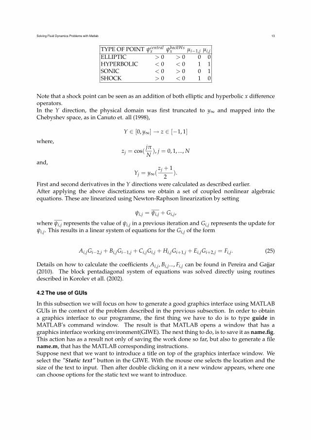
TYPE OF POINT ψcentralx ψbackWs

x µi−1,j µi,jELLIPTIC > 0 > 0 0 0HYPERBOLIC < 0 < 0 1 1SONIC < 0 > 0 0 1SHOCK > 0 < 0 1 0

Note that a shock point can be seen as an addition of both elliptic and hyperbolic x differenceoperators.In the Y direction, the physical domain was first truncated to y∞ and mapped into theChebyshev space, as in Canuto et. all (1998),

Y ∈ [0, y∞]→ z ∈ [−1, 1]

where,

zj = cos(jπN

), j = 0, 1, ..., N

and,

Yj = y∞(zj + 1

2).

First and second derivatives in the Y directions were calculated as described earlier.After applying the above discretizations we obtain a set of coupled nonlinear algebraicequations. These are linearized using Newton-Raphson linearization by setting

ψi,j = ψi,j + Gi,j,

where ψi,j represents the value of ψi,j in a previous iteration and Gi,j represents the update forψi,j. This results in a linear system of equations for the Gi,j of the form

Ai,jGi−2,j + Bi,jGi−1,j + Ci,jGi,j + Hi,jGi+1,j + Ei,jGi+2,j = Fi,j. (25)

Details on how to calculate the coefficients Ai,j, Bi,j..., Fi,j can be found in Pereira and Gajjar(2010). The block pentadiagonal system of equations was solved directly using routinesdescribed in Korolev et all. (2002).

4.2 The use of GUIs

In this subsection we will focus on how to generate a good graphics interface using MATLABGUIs in the context of the problem described in the previous subsection. In order to obtaina graphics interface to our programme, the first thing we have to do is to type guide inMATLAB’s command window. The result is that MATLAB opens a window that has agraphics interface working environment(GIWE). The next thing to do, is to save it as name.fig.This action has as a result not only of saving the work done so far, but also to generate a filename.m, that has the MATLAB corresponding instructions.Suppose next that we want to introduce a title on top of the graphics interface window. Weselect the "Static text" button in the GIWE. With the mouse one selects the location and thesize of the text to input. Then after double clicking on it a new window appears, where onecan choose options for the static text we want to introduce.


Another important feature on the design of an interface, is how to read data from this interface.To do so, one option is to select the "Edit text" button in the GIWE. With the mouse one selectsthe location and the size of the text to be read. Then, after a double click a new windowappears where one can chose options for the text to be read from the keyboard. It is possibleto choose a default text that can be attributed to a certain variable in the MATLAB code. If wefill in the field "Tag" with a name, that can be used to attribute the edited text to a variable.Suppose we fill the field "Tag" with A1. By doing this and saving it, one automatically obtainsin the .m file two new functions A1CreateFcn and A1Callback. The first function executesduring object creation, after setting all properties. The second function allows for the editedtext to be attributed to a variable when the enter key is pressed. Say we want to attribute theedited text to the variable "x", all you have to do is to write in the A1Callback function thefollowing instruction:

x=str2double(get(handles.A1,’String’));

Here, the text read via the keyboard, once the enter key is pressed, is converted to double andattributed to a variable "x". This feature is very important for the user to be able to set thevalues of any variables to be used in the program.

In many codes, it is also very important to define a push button. This can be used to setup certain actions once it is pushed. An example is when one wants to read data from thekeyboard, before starting a simulation. To implement this idea, we click the push button inthe GIWE. Then one selects the size and place where to put it in the GIWE. Next, if one doubleclicks in it, a new window opens and the options for this push button are defined. Once thisis done and it is saved, a new function is created in the .m file called pushbuttonCallback.All the actions that are to happen once the button is pushed are to appear in this function.For instance, one can attribute a set of values to a set of variables. This is done exactly in thesame way as before. The difference is that this can be done to a set of many variables at once.The next instructions we put in this function are the ones that compose the main code of ourprogramme.

Suppose that in the course of the simulation, we want to show a graphic object. This is doneby choosing the Axes button in the GIWE. Then one selects the size and place where to putthe graphic in the GIWE. Next, a double click on it and a new window opens and the optionsfor this Axes button are defined. If we fill in the field "Tag" with a name, say "graphics1", inorder to plot a graphic (x, f (x)) in that window, we would write:

axes(handles.graphics1);plot(x,f)

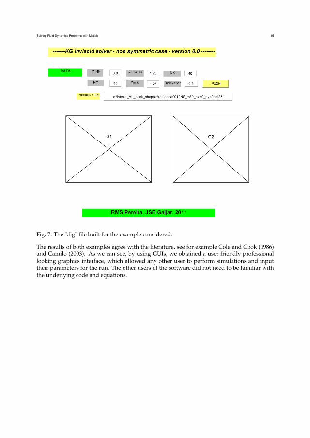
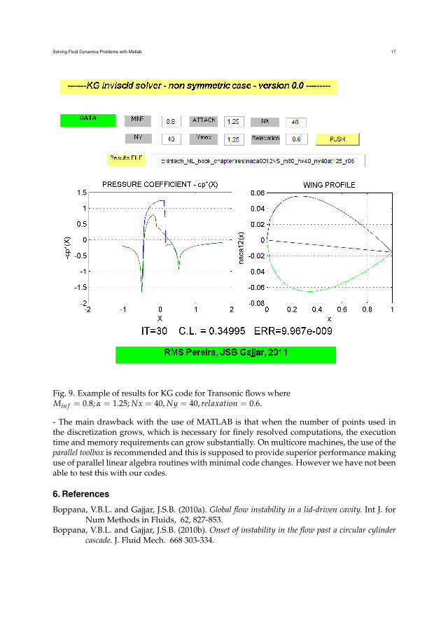
Using these features, we were able to define a useful graphics interface for the programto solve the transonic flow past an airfoil using the mathematical model presented in theprevious section. The interface was built for the NACA0012 airfoil.The parameters considered were: Angle of attack (α), Mach number(M∞), number of pointsin the x direction over the wing (nx), number of points in the Y direction (ny), maximum valuefor Y (Ymax), and relaxation factor (w).In the figures 8, 9, we present the results obtained by our code for two classic examplesextensively studied in the literature. The first example is for M∞ = 0.75, α = 2.0, nx = 40,ny = 40, Ymax = 1.25, w = 0.5.The second example is for M∞ = 0.8, α = 1.25, nx = 40, ny = 40, Ymax = 1.25, w = 0.6.


Fig. 7. The ".fig" file built for the example considered.

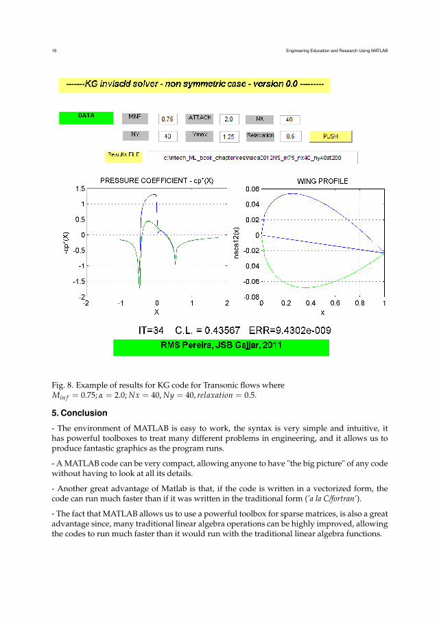
The results of both examples agree with the literature, see for example Cole and Cook (1986)and Camilo (2003). As we can see, by using GUIs, we obtained a user friendly professionallooking graphics interface, which allowed any other user to perform simulations and inputtheir parameters for the run. The other users of the software did not need to be familiar withthe underlying code and equations.


Fig. 8. Example of results for KG code for Transonic flows whereMin f = 0.75; α = 2.0; Nx = 40, Ny = 40, relaxation = 0.5.

5. Conclusion

- The environment of MATLAB is easy to work, the syntax is very simple and intuitive, ithas powerful toolboxes to treat many different problems in engineering, and it allows us toproduce fantastic graphics as the program runs.

- A MATLAB code can be very compact, allowing anyone to have "the big picture" of any codewithout having to look at all its details.

- Another great advantage of Matlab is that, if the code is written in a vectorized form, thecode can run much faster than if it was written in the traditional form (’a la C/fortran’).

- The fact that MATLAB allows us to use a powerful toolbox for sparse matrices, is also a greatadvantage since, many traditional linear algebra operations can be highly improved, allowingthe codes to run much faster than it would run with the traditional linear algebra functions.


Fig. 9. Example of results for KG code for Transonic flows whereMin f = 0.8; α = 1.25; Nx = 40, Ny = 40, relaxation = 0.6.

- The main drawback with the use of MATLAB is that when the number of points used inthe discretization grows, which is necessary for finely resolved computations, the executiontime and memory requirements can grow substantially. On multicore machines, the use of theparallel toolbox is recommended and this is supposed to provide superior performance makinguse of parallel linear algebra routines with minimal code changes. However we have not beenable to test this with our codes.

6. References

Boppana, V.B.L. and Gajjar, J.S.B. (2010a). Global flow instability in a lid-driven cavity. Int J. forNum Methods in Fluids, 62, 827-853.

Boppana, V.B.L. and Gajjar, J.S.B. (2010b). Onset of instability in the flow past a circular cylindercascade. J. Fluid Mech. 668 303-334.


Camilo E. (2003). Solução numérica das equações de Euler para representação do escoamentotransónico de aerofólios.M.Sc thesis, University of São Paulo, Brazil.

Canuto, C., Hussaini, M. Y., Quarteroni, A. and Zhang, T.A., (1998). Spectral Methods in FluidMechanics. Springer series in Comp. Phys., Springer Verlag.

Cole, J. D. and Cook, L. P., (1986). Transonic Aerodynamics, Elsevier Science Publishers B.V. .Korolev G.L, Gajjar J.S.B., and Ruban A.I., (2002). Once again on the supersonic flow separation

near a corner. J. Fluid Mech., 463, 173-199.Mizushima, J. and Ino, Y., (2008). Stability of flows past a pair of circular cylinders in a side-by-side

arrangement. J. Fluid Mech., 595, 491-507.Murman, E. M. and Cole, J. D.,(1971). Calculation of plane steady transonic flows. Boeing Scientific

Research Laboratories.Pereira, R. M. S. and Gajjar, J. S. B. (2010). Transonic Inviscid Flows Past Thin Airfoils: A New

Numerical Method and Global Stability Analysis using MatLab. International Journal ofMathematical Models and Methods in Applied Sciences, ISSN 1998-0140.

Trefethen L.N., (2000). Spectral Methods in Matlab. SIAM.Weideman, J.A.C and Reddy, S.C (2003). http://dip.sun.ac.za/∼weideman/research/differ.html .

solving fluid dynamics problems with matlab · pdf filematlab allows us to use a powerful...

Documents