solving a large-scale precedence constrained scheduling problem with elastic jobs using tabu search
TRANSCRIPT
Computers & Operations Research 34 (2007) 2025–2042www.elsevier.com/locate/cor
Solving a large-scale precedence constrained scheduling problemwith elastic jobs using tabu search
Christian R. Pedersena,∗, Rasmus V. Rasmussena,∗, Kim A. Andersenb
aDepartment of Operations Research, University of Aarhus, Ny Munkegade, Building 530, 8000 Aarhus C, DenmarkbDepartment of Accounting, Finance and Logistics, Aarhus School of Business, Fuglesangs Allé 4, 8210 Aarhus V, Denmark
Available online 3 October 2005
Abstract
This paper presents a solution method for minimizing makespan of a practical large-scale scheduling problemwith elastic jobs. The jobs are processed on three servers and restricted by precedence constraints, time windowsand capacity limitations. We derive a new method for approximating the server exploitation of the elastic jobs andsolve the problem using a tabu search procedure. Finding an initial feasible solution is in general NP-complete, butthe tabu search procedure includes a specialized heuristic for solving this problem. The solution method has provento be very efficient and leads to a significant decrease in makespan compared to the strategy currently implemented.� 2005 Elsevier Ltd. All rights reserved.
Keywords: Large-scale scheduling; Elastic jobs; Precedence constraints; Practical application; Tabu search
1. Introduction
This paper focuses on a specific problem provided to us by the Danish telecommunications net operator,Sonofon. By the end of each day a rather large number of jobs (End-of-Day jobs) have to be processed onthree available servers. Each job is preassigned to one of the three servers and the objective is to schedulethe jobs on the machines in order to minimize makespan. This task is complicated by the fact that a largenumber of precedence constraints among the jobs must be fulfilled, that time windows must be obeyed
∗ Corresponding authors. Tel.: +45 8942 3536; fax: +45 8613 1769.E-mail addresses: [email protected] (C.R. Pedersen), [email protected] (R.V. Rasmussen), [email protected] (K. A. Andersen).
0305-0548/$ - see front matter � 2005 Elsevier Ltd. All rights reserved.doi:10.1016/j.cor.2005.08.001
2026 C.R. Pedersen et al. / Computers & Operations Research 34 (2007) 2025–2042
and that capacity limitations must be respected. In addition, the jobs are elastic which means that theduration of a particular job depends on the capacity assigned to the job. Elasticity of jobs complicatesthe problem considerably and has to the best of our knowledge not yet been considered in large-scalescheduling.
The applications of scheduling problems are wide-spread, and hence a considerable amount of promis-ing research has been devoted to such problems both within the operations research literature and thecomputer science literature. Especially during the past decade algorithms merging operations researchtechniques and constraint programming (CP) have proved efficient as exact solution methods for solv-ing scheduling problems. Among a number of interesting CP contributions to small- or medium-scaledscheduling problems we mention the work by Jain and Grossmann [1], Hooker and Ottoson [2], Hooker[3] and Baptiste et al. [4,5]. For large-scale problems, meta heuristics in particular have shown promisingresults.
One classical meta heuristic that has been successfully applied to scheduling problems is tabu search,due to Glover [6] and Glover and Laguna [7]. The papers on tabu search are numerous, but let us forbrevity only mention a few which all appeared recently and consider scheduling problems. Grabowskiand Wodecki [8] consider large-scale flow shop problems with makespan criterion and develop a veryfast tabu search heuristic focusing on a lower bound for the makespan instead of the exact makespanvalue. Ferland et al. [9] consider a practical problem of scheduling internships for physician studentsand propose several variants of tabu search procedures. The last three papers all consider the problemof scheduling a number of jobs to a set of heterogeneous machines under precedence constraints, withthe objective of minimizing makespan. In Porto et al. [10] a parallel Tabu Search heuristic is developedand proved superior to a widely used greedy heuristic for the problem. In Chekuri and Bender [11]a new approximation algorithm is presented, but unfortunately, no computational results are reported.Finally, in Mansini et al. [12] jobs with up to three predecessors each are considered among groupsof jobs requiring the same set of machines. The problem is formulated as a graph-theoretical prob-lem. In the paper a number of approximation results are provided, but no computational experience isreported.
Clearly, the vast solution space and the complexity of the present problem called for a heuristic pro-cedure. Due to the high flexibility of tabu search and its promising results with scheduling problems, wechose that method.
The contributions of this paper can be summarized as follows:
• We present a special designed heuristic based on tabu search to solve a large-scale practical prob-lem provided to us by a large Danish telecommunications net operator, Sonofon. Today Sonofonfaces the problem that the average completion time exceeds the deadline by 41 min. This meansthat with the existing scheduling strategy new hardware needs to be purchased in order to keepsatisfying the given requirements. This paper shows that the existing hardware is, in fact, suffi-cient to complete the jobs in time and indeed spare capacity is available, when a good schedule ischosen.
• The algorithm is capable of handling large-scale scheduling problems with precedence constraintsamong jobs and time windows, and a new approximate method for scheduling elastic jobs isdeveloped.
• A heuristic procedure for obtaining an initial feasible solution is provided. This proves to work verywell on the specific application which cannot be solved by traditional IP/CP code.
C.R. Pedersen et al. / Computers & Operations Research 34 (2007) 2025–2042 2027
• The solution method provides a significant improvement in makespan compared to the strategy cur-rently implemented by Sonofon, and an improvement of 25 percent to the current solution is reportedwithin 56 min of computation time. Sonofon expects to use the proposed solution method in thefuture.
• The algorithm quickly finds a good solution and can be aborted at any time. Therefore as long as thejobs are known just prior to the actual scheduling process our algorithm is capable of producing agood feasible schedule.
The remaining part of the paper is organized as follows. In Section 2, we present the practical prob-lem offered by Sonofon, followed by the derivation of a hybrid IP/CP model. In Section 3, we give athorough introduction to the developed tabu search heuristic, and computational results are provided inSection 4.
2. Problem formulation
The Danish telecommunications net operator, Sonofon, faces a three-machine scheduling problem,with 346 End-of-Day jobs (EOD). Each job is dedicated to a particular server in advance and it has to beprocessed on that server without preemption.1 This means that the allocation of jobs to machines is notpart of the problem.
The scheduling time horizon runs from 7.00 p.m. to 8.00 a.m., and each job receives a time win-dow in which it should be processed. The time windows are wide, leaving numerous feasible start-ing times for each job. Since most scheduling tools applying Constraint Programming rely heavily onpropagation techniques, the wide time windows have a negative influence on the performance of suchscheduling packages. The time windows will be explored further in Section 3.1. Since the servers imme-diately after completing the EOD-jobs are assigned to other operations, the objective will be to minimizemakespan.
Because of interrelations between jobs, a number of precedence constraints must be fulfilled. It mightoccur that a job need information from a database to which another job (a predecessor) has writtenearlier.
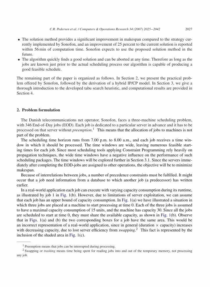
In a real-world application each job can execute with varying capacity consumption during its runtime,as illustrated by job 1 in Fig. 1(b). However, due to limitations of server exploitation, we can assumethat each job has an upper bound of capacity consumption. In Fig. 1(a) we have illustrated a situation inwhich three jobs are placed at a machine to start processing at time 0. Each of the three jobs is assumedto have a maximal capacity consumption of 15 units, and the machine has capacity 30. Since all the jobsare scheduled to start at time 0, they must share the available capacity, as shown in Fig. 1(b). Observethat in Figs. 1(a) and (b) the two corresponding boxes for a job have the same area. This would bean incorrect representation of a real-world application, since in general (duration × capacity) increaseswith decreasing capacity, due to lost server efficiency from swapping.2 This fact is represented by theinclusion of the shaded area in Fig. 1(c).
1 Preemption means that jobs can be interrupted during processing.2 Swapping or trashing means time being spent for reading jobs into and out of the temporary memory, not processing
any job.
2028 C.R. Pedersen et al. / Computers & Operations Research 34 (2007) 2025–2042
0
10
20
30
40
0 10 20 30 40
capa
city
time(a)
job1
job2
job3
0
10
20
30
40
0 10 20 30 40
capa
city
0
10
20
30
40
capa
city
time(b)
job1
job2
job3
0 10 20 30 40time(c)
job1
job2
job3
Fig. 1. (Duration × capacity) increases with decreasing capacity.
0
5
10
15
20
0 10 15 20 25
capa
city
time
box1
box2
box3
5
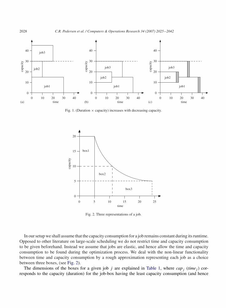
Fig. 2. Three representations of a job.
In our setup we shall assume that the capacity consumption for a job remains constant during its runtime.Opposed to other literature on large-scale scheduling we do not restrict time and capacity consumptionto be given beforehand. Instead we assume that jobs are elastic, and hence allow the time and capacityconsumption to be found during the optimization process. We deal with the non-linear functionalitybetween time and capacity consumption by a rough approximation representing each job as a choicebetween three boxes, (see Fig. 2).
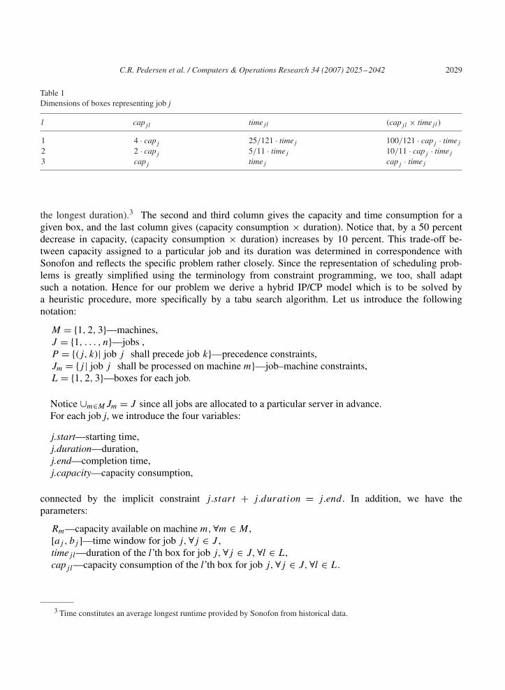
The dimensions of the boxes for a given job j are explained in Table 1, where capj (timej ) cor-responds to the capacity (duration) for the job-box having the least capacity consumption (and hence
C.R. Pedersen et al. / Computers & Operations Research 34 (2007) 2025–2042 2029
Table 1Dimensions of boxes representing job j
l capj l timej l (capj l × timej l)
1 4 · capj 25/121 · timej 100/121 · capj · timej
2 2 · capj 5/11 · timej 10/11 · capj · timej
3 capj timej capj · timej
the longest duration).3 The second and third column gives the capacity and time consumption for agiven box, and the last column gives (capacity consumption × duration). Notice that, by a 50 percentdecrease in capacity, (capacity consumption × duration) increases by 10 percent. This trade-off be-tween capacity assigned to a particular job and its duration was determined in correspondence withSonofon and reflects the specific problem rather closely. Since the representation of scheduling prob-lems is greatly simplified using the terminology from constraint programming, we too, shall adaptsuch a notation. Hence for our problem we derive a hybrid IP/CP model which is to be solved bya heuristic procedure, more specifically by a tabu search algorithm. Let us introduce the followingnotation:
M = {1, 2, 3}—machines,J = {1, . . . , n}—jobs ,P = {(j, k)| job j shall precede job k}—precedence constraints,Jm = {j | job j shall be processed on machine m}—job–machine constraints,L = {1, 2, 3}—boxes for each job.
Notice ∪m∈MJm = J since all jobs are allocated to a particular server in advance.For each job j, we introduce the four variables:
j.start—starting time,j.duration—duration,j.end—completion time,j.capacity—capacity consumption,
connected by the implicit constraint j.start + j.duration = j.end. In addition, we have theparameters:
Rm—capacity available on machine m, ∀m ∈ M ,[aj , bj ]—time window for job j, ∀j ∈ J ,timej l—duration of the l’th box for job j, ∀j ∈ J, ∀l ∈ L,capj l—capacity consumption of the l’th box for job j, ∀j ∈ J, ∀l ∈ L.
3 Time constitutes an average longest runtime provided by Sonofon from historical data.
2030 C.R. Pedersen et al. / Computers & Operations Research 34 (2007) 2025–2042
Let xjl denote a binary variable which is 1 if box l is chosen for job j and 0 otherwise. Introducing theartificial job makespan with zero duration, we can state our model as follows:
min makespan.end
s.t.∑l∈L
xjl = 1 ∀j ∈ J , (1)
j.duration =∑l∈L
(xjl · timej l) ∀j ∈ J , (2)
j.capacity =∑l∈L
(xjl · capj l) ∀j ∈ J , (3)
aj � j.start ∀j ∈ J , (4)j.end�bj ∀j ∈ J , (5)j precedes makespan ∀j ∈ J , (6)j precedes k ∀(j, k) ∈ P , (7)
cumulative
⎛⎜⎝
{j.start}j∈Jm{j.duration}j∈Jm{j.capacity}j∈Jm
Rm
⎞⎟⎠ ∀m ∈ M , (8)
xjl ∈ {0, 1} ∀j ∈ J, ∀l ∈ L, (9)
where cumulative is a global constraint in CP, stating that, at all times, the total capacity is not exceededby the capacity consumption of running jobs. The constraint can be rewritten as
cumulative ((t1, . . . , tn), (d1, . . . , dn), (r1, . . . , rn), R)
� ∑{j |tj � t � tj+dj }
rj �R ∀t ,
where the vector (t1, . . . , tn) represents starting times of jobs 1, . . . , n, with duration (d1, . . . , dn) andcapacity consumption (r1, . . . , rn). Available capacity is R.
The above constraints (1) choose a box for each job, yielding a specific time and capacity consumptionin cooperation with (2) and (3). Constraints (4) and (5) consider time windows. Constraints (6) togetherwith the objective function minimize the completion time of the last job. Constraints (7) handle precedenceconstraints (j precedes k means j.end �k.start), whereas constraints (8) handle resource consumptionfor each machine.
3. Tabu search
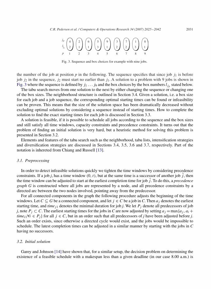
To obtain a solution to the given problem we need the starting time and the box size for each jobsince then the completion times, the durations and the capacity consumptions are implicitly determined.However, due to wide time windows numerous possible starting times exist for each job and prevent usfrom using the starting times explicitly in the solutions. Instead a solution is composed of a box size foreach job and a sequence which specifies the order of the starting times. Given a sequence we let jp denote
C.R. Pedersen et al. / Computers & Operations Research 34 (2007) 2025–2042 2031
1 9
4
2 1
jp
ljp
p 2 3 4 5 6 7 8
1 1 3 1 2 2 3
2 6 5 9 3 7 1 8
Fig. 3. Sequence and box choices for example with nine jobs.
the number of the job at position p in the following. The sequence specifies that since job j1 is beforejob j2 in the sequence, j2 must start no earlier than j1. A solution to a problem with 9 jobs is shown inFig. 3 where the sequence is defined by j1 . . . j9 and the box choices by the box numbers ljp stated below.
The tabu search moves from one solution to the next by either changing the sequence or changing oneof the box sizes. The neighborhood structure is outlined in Section 3.4. Given a solution, i.e. a box sizefor each job and a job sequence, the corresponding optimal starting times can be found or infeasibilitycan be proven. This means that the size of the solution space has been dramatically decreased withoutexcluding optimal solutions by considering a sequence instead of starting times. How to complete thesolution to find the exact starting times for each job is discussed in Section 3.3.
A solution is feasible, if it is possible to schedule all jobs according to the sequence and the box sizesand still satisfy all time windows, capacity constraints and precedence constraints. It turns out that theproblem of finding an initial solution is very hard, but a heuristic method for solving this problem ispresented in Section 3.2.
Elements and features of the tabu search such as the neighborhood, tabu lists, intensification strategiesand diversification strategies are discussed in Sections 3.4, 3.5, 3.6 and 3.7, respectively. Part of thenotation is inhereted from Chiang and Russell [13].
3.1. Preprocessing
In order to detect infeasible solutions quickly we tighten the time windows by considering precedenceconstraints. If a job j, has a time window (0, t), but at the same time is a successor of another job j , thenthe time window can be adjusted to start at the earliest completion time for job j . To do this, a precedencegraph G is constructed where all jobs are represented by a node, and all precedence constraints by adirected arc between the two nodes involved, pointing away from the predecessor.
For all connected components in the graph the following procedure adjusts the beginning of the timewindows. Let C ⊆ G be a connected component, and let j ∈ C be a job in C. Then aj denotes the earlieststarting time, and timej1 denotes the minimal duration for job j. We let Pj denote all predecessors of jobj, note Pj ⊂ C. The earliest starting times for the jobs in C are now adjusted by setting aj =max{aj , ai +timei1∀i ∈ Pj } for all j ∈ C, but in an order such that all predecessors of j have been adjusted before j.Such an order exists, since otherwise a directed cycle would exist, and the jobs would be impossible toschedule. The latest completion times can be adjusted in a similar manner by starting with the jobs in Chaving no successors.
3.2. Initial solution
Garey and Johnson [14] have shown that, for a similar setup, the decision problem on determining theexistence of a feasible schedule with a makespan less than a given deadline (in our case 8.00 a.m.) is
2032 C.R. Pedersen et al. / Computers & Operations Research 34 (2007) 2025–2042
job 1
job 2
job 3 job 5 job 6
job 7
time
t1 t2 t3 t4
layer 1: job 1, job 2, job 3
layer 2: job 4
layer 3: job 5
layer 4: job 6, job 7
(a) (b)
job 4
Fig. 4. How jobs are divided into layers.
NP-complete in the strong sense. In this section, we shall describe a heuristical procedure to generate aninitial feasible solution for this particular instance. The procedure is divided into five steps where the firstthree steps use the precedence graph to generate a sequence. In the fourth step, box sizes are chosen. Ifthe solution obtained is feasible the procedure stops, and otherwise Step 5 relaxes the problem and usesthe tabu search to find a feasible solution.
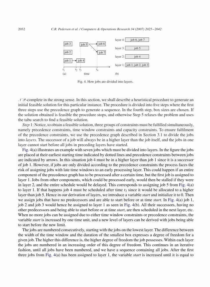
Step 1: Notice, to obtain a feasible solution, three groups of constraints must be fulfilled simultaneously,namely precedence constraints, time window constraints and capacity constraints. To ensure fulfilmentof the precedence constraints, we use the precedence graph described in Section 3.1 to divide the jobsinto layers. The successor of a job will always be in a higher layer than the job itself, and the jobs in onelayer cannot start before all jobs in preceding layers have started.
Fig. 4(a) illustrates an example with seven jobs which must be divided into layers. In the figure the jobsare placed at their earliest starting time indicated by dotted lines and precedence constraints between jobsare indicated by arrows. In this situation job 4 must be in a higher layer than job 1 since it is a successorof job 1. However, if jobs are only divided according to the precedence constraints the process faces therisk of assigning jobs with late time windows to an early processing layer. This could happen if an entirecomponent of the precedence graph has to be processed after a certain time, but the first job is assigned tolayer 1. Jobs from other components, which could be processed early, would then be stalled if they werein layer 2, and the entire schedule would be delayed. This corresponds to assigning job 5 from Fig. 4(a)to layer 1. If that happens job 4 must be scheduled after time t3 since it would be allocated to a higherlayer than job 5. Hence in our derivation of layers, we introduce a variable start and initialize it to 0. Thenwe assign jobs that have no predecessors and are able to start before or at time start. In Fig. 4(a) job 1,job 2 and job 3 would hence be assigned to layer 1 as seen in Fig. 4(b). All their successors, having noother predecessors and being able to start before or at time start, are then scheduled in the next layer, etc.When no more jobs can be assigned due to either time window constraints or precedence constraints, thevariable start is increased by one time unit, and a new level of layers can be derived with jobs being ableto start before the new limit.
The jobs are numbered consecutively, starting with the jobs on the lowest layer. The difference betweenthe width of the time window and the duration of the smallest box expresses a degree of freedom for agiven job. The higher this difference is, the higher degree of freedom the job possesses. Within each layerthe jobs are numbered in an increasing order of this degree of freedom. This continues in an iterativefashion, until all jobs have been numbered, and we have a sequence containing all jobs. After the firstthree jobs from Fig. 4(a) has been assigned to layer 1, the variable start is increased until it is equal to
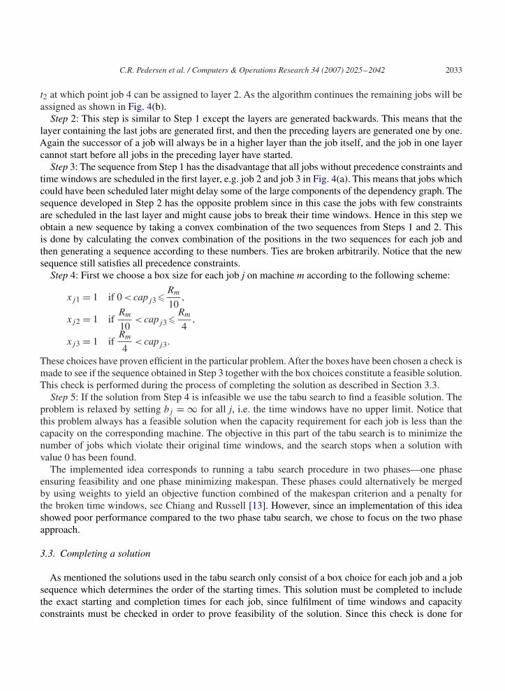
C.R. Pedersen et al. / Computers & Operations Research 34 (2007) 2025–2042 2033
t2 at which point job 4 can be assigned to layer 2. As the algorithm continues the remaining jobs will beassigned as shown in Fig. 4(b).
Step 2: This step is similar to Step 1 except the layers are generated backwards. This means that thelayer containing the last jobs are generated first, and then the preceding layers are generated one by one.Again the successor of a job will always be in a higher layer than the job itself, and the job in one layercannot start before all jobs in the preceding layer have started.
Step 3: The sequence from Step 1 has the disadvantage that all jobs without precedence constraints andtime windows are scheduled in the first layer, e.g. job 2 and job 3 in Fig. 4(a). This means that jobs whichcould have been scheduled later might delay some of the large components of the dependency graph. Thesequence developed in Step 2 has the opposite problem since in this case the jobs with few constraintsare scheduled in the last layer and might cause jobs to break their time windows. Hence in this step weobtain a new sequence by taking a convex combination of the two sequences from Steps 1 and 2. Thisis done by calculating the convex combination of the positions in the two sequences for each job andthen generating a sequence according to these numbers. Ties are broken arbitrarily. Notice that the newsequence still satisfies all precedence constraints.
Step 4: First we choose a box size for each job j on machine m according to the following scheme:
xj1 = 1 if 0 < capj3 �Rm
10,
xj2 = 1 ifRm
10< capj3 �
Rm
4,
xj3 = 1 ifRm
4< capj3.
These choices have proven efficient in the particular problem. After the boxes have been chosen a check ismade to see if the sequence obtained in Step 3 together with the box choices constitute a feasible solution.This check is performed during the process of completing the solution as described in Section 3.3.
Step 5: If the solution from Step 4 is infeasible we use the tabu search to find a feasible solution. Theproblem is relaxed by setting bj = ∞ for all j, i.e. the time windows have no upper limit. Notice thatthis problem always has a feasible solution when the capacity requirement for each job is less than thecapacity on the corresponding machine. The objective in this part of the tabu search is to minimize thenumber of jobs which violate their original time windows, and the search stops when a solution withvalue 0 has been found.
The implemented idea corresponds to running a tabu search procedure in two phases—one phaseensuring feasibility and one phase minimizing makespan. These phases could alternatively be mergedby using weights to yield an objective function combined of the makespan criterion and a penalty forthe broken time windows, see Chiang and Russell [13]. However, since an implementation of this ideashowed poor performance compared to the two phase tabu search, we chose to focus on the two phaseapproach.
3.3. Completing a solution
As mentioned the solutions used in the tabu search only consist of a box choice for each job and a jobsequence which determines the order of the starting times. This solution must be completed to includethe exact starting and completion times for each job, since fulfilment of time windows and capacityconstraints must be checked in order to prove feasibility of the solution. Since this check is done for
2034 C.R. Pedersen et al. / Computers & Operations Research 34 (2007) 2025–2042
0
10
20
(a)
ajpajp
ajpajp
jp− 1.start jp− 1.start jp− 1.start jp− 1.start
capa
city
0
10
20
capa
city
0
10
20
capa
city
0
10
20
capa
city
time
job jp-1
job jp−2
job jp
(b) time
job jp−1
job jp−2
(c) (d) timetime
pre. con.job jp−2 job jp−2
job jp job jp job jp
job jp−1 job jp−1
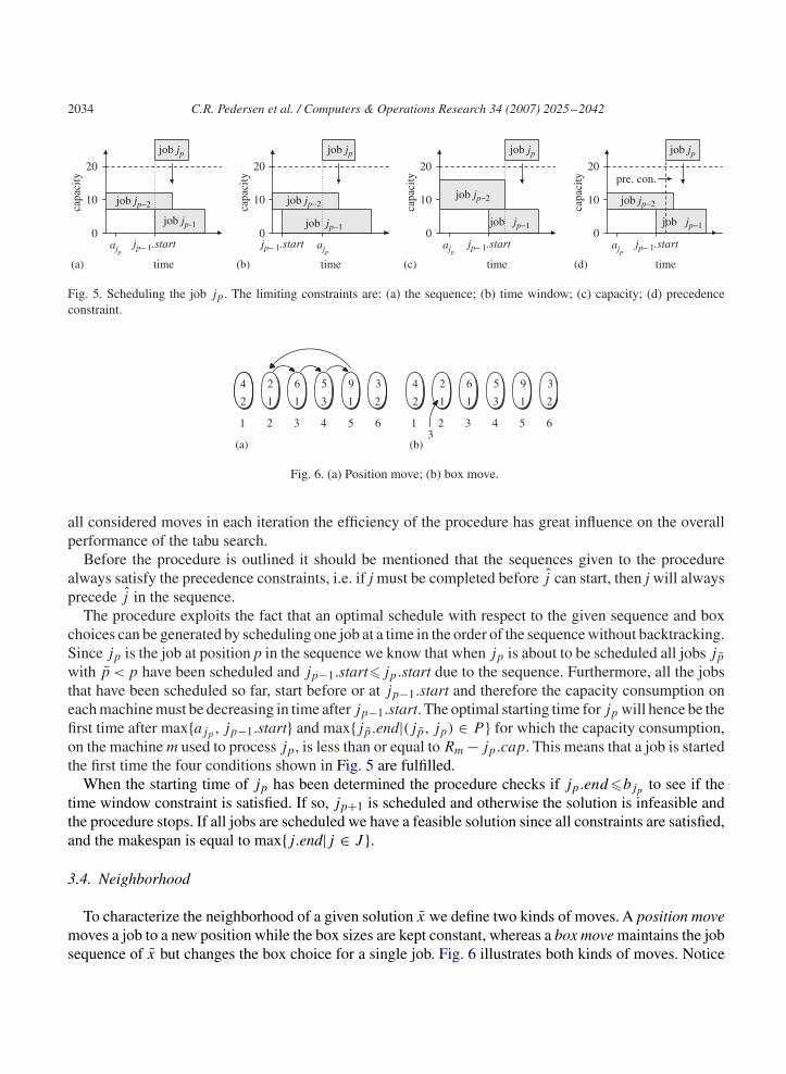
Fig. 5. Scheduling the job jp . The limiting constraints are: (a) the sequence; (b) time window; (c) capacity; (d) precedenceconstraint.
3(a) (b)
1
4
2
2 3 4 5 6 1 2 3 4 5 6
1 1 3 1 2
2 6 5 9 3 4
2 1 1 3 1 2
2 6 5 9 3
Fig. 6. (a) Position move; (b) box move.
all considered moves in each iteration the efficiency of the procedure has great influence on the overallperformance of the tabu search.
Before the procedure is outlined it should be mentioned that the sequences given to the procedurealways satisfy the precedence constraints, i.e. if j must be completed before j can start, then j will alwaysprecede j in the sequence.
The procedure exploits the fact that an optimal schedule with respect to the given sequence and boxchoices can be generated by scheduling one job at a time in the order of the sequence without backtracking.Since jp is the job at position p in the sequence we know that when jp is about to be scheduled all jobs jp
with p < p have been scheduled and jp−1.start�jp.start due to the sequence. Furthermore, all the jobsthat have been scheduled so far, start before or at jp−1.start and therefore the capacity consumption oneach machine must be decreasing in time after jp−1.start. The optimal starting time for jp will hence be thefirst time after max{ajp , jp−1.start} and max{jp.end|(jp, jp) ∈ P } for which the capacity consumption,on the machine m used to process jp, is less than or equal to Rm − jp.cap. This means that a job is startedthe first time the four conditions shown in Fig. 5 are fulfilled.
When the starting time of jp has been determined the procedure checks if jp.end �bjp to see if thetime window constraint is satisfied. If so, jp+1 is scheduled and otherwise the solution is infeasible andthe procedure stops. If all jobs are scheduled we have a feasible solution since all constraints are satisfied,and the makespan is equal to max{j.end|j ∈ J }.
3.4. Neighborhood
To characterize the neighborhood of a given solution x we define two kinds of moves. A position movemoves a job to a new position while the box sizes are kept constant, whereas a box move maintains the jobsequence of x but changes the box choice for a single job. Fig. 6 illustrates both kinds of moves. Notice
C.R. Pedersen et al. / Computers & Operations Research 34 (2007) 2025–2042 2035
in Fig. 6(a) that, when job 9 at position 5 in the job sequence is moved to position 2, not only does job 9get a new position, but the jobs at position 2, 3 and 4 are moved to the subsequent position.
The position move described above has been chosen instead of alternatives, such as exchanging twojobs, since the precedence constraints does not limit the flexibility of this move. Consider the move fromFig. 6(a) and imagine that job 2 must precede job 6 and job 6 must precede job 5. In that case three“exchanges” of jobs are needed to perform the single position move shown in the figure.
The neighborhood for solution x can be characterized as the union of solutions obtained by a singlebox move and solutions obtained by a single position move which fulfils the precedence constraints. Thecardinality of the neighborhood is O(n2) due to the large number of position moves, and in the presentimplementation we must consider approximately 120,000 moves (some are ignored due to violation ofthe precedence constraints) for each solution. The ability to select only part of the neighborhood forexamination is therefore crucial. We use two methods for limiting the number of possible moves.
3.4.1. Restricting position movesBy introducing a limit movelimit on how far a job can move, the number of considered position moves
are reduced. This leads to faster iterations but might restrict the search from choosing some very goodsolutions. To avoid the search from stalling due to the restriction, the entire neighborhood is examinedevery time the algorithm has performed non-improving moves for a predefined number of iterations.This makes the search capable of performing a single time consuming move and then a number of fastiterations to exploit the new conditions.
3.4.2. Candidate listsThe Elite Candidate List approach (see [7]), is used to limit the number of position moves by only
evaluating moves belonging to candidate lists. In this setup two lists are used, and they are constructed byevaluating the neighborhood of the initial solution. All moves which lead to an improving makespan arestored in list 1, and all moves leading to the same makespan are stored in list 2. In the following iterationsonly moves from the two candidate lists are considered. First the moves in list 1 are evaluated, and if oneof these moves leads to an improving makespan the best move is chosen. If list 1 does not contain animproving move the moves in list 2 are evaluated, and the best move considering both list 1 and list 2 ischosen.
When a move has been chosen from one of the candidate lists both lists are updated by deleting allmoves conflicting with the chosen one. This means that, if a position move for job j is chosen, then allother position moves for job j are deleted from the candidate lists and correspondingly for box moves.The candidate lists are used until no improving move has been found in the lists. When this happens bothlists are deleted, and two new lists are generated by examining the possible moves of the current solution.Notice that, this might not be an evaluation of all possible moves, since the position moves might berestricted as explained in Section 3.4.1. The underlying assumption of the strategy is that a move whichperforms well in the current solution will probably also lead to improvements in the following iterations.
3.5. Tabu list
The corner stone in tabu search is the use of short-term memory by generating a tabu list. The tabulist stores the move from an iteration and keeps it for TimeInTL iterations. This is done by keeping theiteration number i from the iteration in which the move is made tabu and deleting the move from the tabu
2036 C.R. Pedersen et al. / Computers & Operations Research 34 (2007) 2025–2042
list when the iteration number exceeds i + TimeInTL. The tabu list differentiates between the two kindsof moves, but the number of the job involved is always stored. If a box move is performed for job j thetabu list restricts job j from performing a new box move in the following TimeInTL iterations, unless theaspiration criterion is satisfied. If a position move is moving job j from position p the tabu list restrictsthe search from performing a new position move taking job j to a position p where |p− p|� tabuPosLimitin the following TimeInTL iterations, unless the aspiration criterion is satisfied.
The aspiration criterion implemented checks if an improved makespan can be obtained by performinga forbidden move. If this is the case the tabu restriction is suspended, and the search is allowed to performthe move.
The tabu search implemented here has the ability to dynamically adjust the variable TimeInTL whichdetermines the number of iterations for which a move is tabu. TimeInTL is decreased by the parameterzdecrease=0.9 every time the search is trapped in a solution without a non-tabu or feasible neighbor andincreased by zincrease = 1.1, when the same makespan has been found in many successive iterations.
In addition a variable steps is counting the number of moves without a change in TimeInTL, andTimeInTL is decreased by zdecrease if steps exceeds a fixed threshold movingaverage. This adjustmenthelps the search to avoid a lot of bad moves which could be the result of a long tabu list.
3.6. Intensification strategy
A list IntenArray holds moves which have led to improvements of the makespan. The moves are keptfor Intensize iterations, and corresponding moves for the same job are not allowed while the move isin the IntenArray. For example, if a position move is performed for job j in iteration i, a new positionmove cannot be performed for j before iteration i + Intensize. However, the intensification status is notconsidered if a job satisfies the aspiration criterion. In this case the job can be chosen even though themove is in the intensification array.
3.7. Diversification strategies
The algorithm contains two kinds of diversification strategies. The first strategy is active throughout thesearch and helps the algorithm to perform a thorough search in the current region of the solution space,while the other strategy forces the search to change the region.
3.7.1. Penalized move valueThe quality of a move is measured by movevalue, which gives the difference between the current
makespan and the makespan obtained by performing the move, movevalue = newTime − curTime. Thismovevalue could be used to guide the search, but in order to implement the first diversification strategy apenalized move value, pmv is introduced. The pmv takes into account how many times the job has beenmoved before:
pmv ={
movevalue + � · Move[j ] if movevalue�0,
movevalue if movevalue < 0,
where Move[j ] counts the number of moves performed by job j and � is a parameter to adjust the penalty.By choosing moves according to lowest pmv, the algorithm automatically follows the diversificationstrategy.
C.R. Pedersen et al. / Computers & Operations Research 34 (2007) 2025–2042 2037
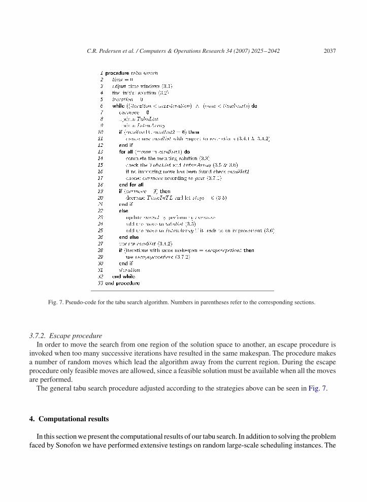
Fig. 7. Pseudo-code for the tabu search algorithm. Numbers in parentheses refer to the corresponding sections.
3.7.2. Escape procedureIn order to move the search from one region of the solution space to another, an escape procedure is
invoked when too many successive iterations have resulted in the same makespan. The procedure makesa number of random moves which lead the algorithm away from the current region. During the escapeprocedure only feasible moves are allowed, since a feasible solution must be available when all the movesare performed.
The general tabu search procedure adjusted according to the strategies above can be seen in Fig. 7.
4. Computational results
In this section we present the computational results of our tabu search. In addition to solving the problemfaced by Sonofon we have performed extensive testings on random large-scale scheduling instances. The
2038 C.R. Pedersen et al. / Computers & Operations Research 34 (2007) 2025–2042
mak
espa
n
time (sec.)
Lower bound
(4.00 am) 540
(5.00 am) 600
(6.00 am) 660
(7.00 am) 720
(8.00 am) 780
1000 2000 3000 4000 5000 6000 7000 8000 9000 10000 11000
current sol.best sol.
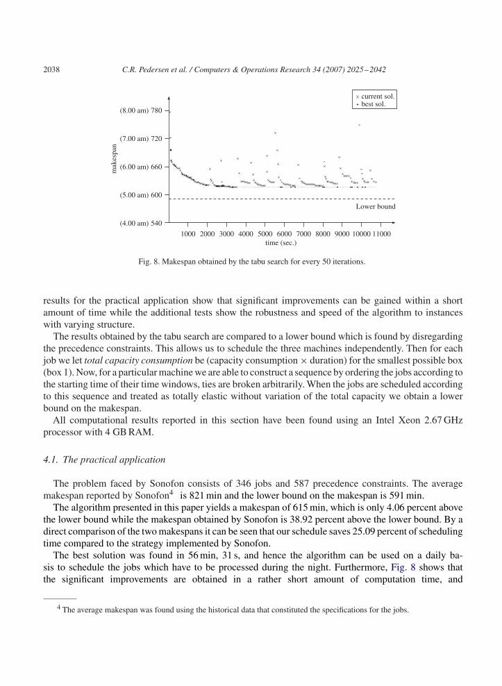
Fig. 8. Makespan obtained by the tabu search for every 50 iterations.
results for the practical application show that significant improvements can be gained within a shortamount of time while the additional tests show the robustness and speed of the algorithm to instanceswith varying structure.
The results obtained by the tabu search are compared to a lower bound which is found by disregardingthe precedence constraints. This allows us to schedule the three machines independently. Then for eachjob we let total capacity consumption be (capacity consumption × duration) for the smallest possible box(box 1). Now, for a particular machine we are able to construct a sequence by ordering the jobs according tothe starting time of their time windows, ties are broken arbitrarily. When the jobs are scheduled accordingto this sequence and treated as totally elastic without variation of the total capacity we obtain a lowerbound on the makespan.
All computational results reported in this section have been found using an Intel Xeon 2.67 GHzprocessor with 4 GB RAM.
4.1. The practical application
The problem faced by Sonofon consists of 346 jobs and 587 precedence constraints. The averagemakespan reported by Sonofon4 is 821 min and the lower bound on the makespan is 591 min.
The algorithm presented in this paper yields a makespan of 615 min, which is only 4.06 percent abovethe lower bound while the makespan obtained by Sonofon is 38.92 percent above the lower bound. By adirect comparison of the two makespans it can be seen that our schedule saves 25.09 percent of schedulingtime compared to the strategy implemented by Sonofon.
The best solution was found in 56 min, 31 s, and hence the algorithm can be used on a daily ba-sis to schedule the jobs which have to be processed during the night. Furthermore, Fig. 8 shows thatthe significant improvements are obtained in a rather short amount of computation time, and
4 The average makespan was found using the historical data that constituted the specifications for the jobs.
C.R. Pedersen et al. / Computers & Operations Research 34 (2007) 2025–2042 2039
0
5
10
15
20
19 24 04 08
capa
city
0
5
10
15
20
capa
city
0
5
10
15
20
capa
city
timeMachine 1 Machine 2 Machine 3
19 24 04 08time
19 24 04 08time
(a) (b) (c)
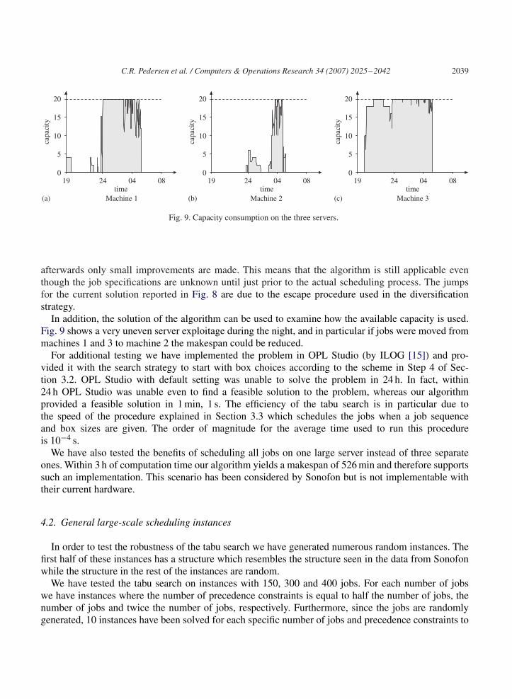
Fig. 9. Capacity consumption on the three servers.
afterwards only small improvements are made. This means that the algorithm is still applicable eventhough the job specifications are unknown until just prior to the actual scheduling process. The jumpsfor the current solution reported in Fig. 8 are due to the escape procedure used in the diversificationstrategy.
In addition, the solution of the algorithm can be used to examine how the available capacity is used.Fig. 9 shows a very uneven server exploitage during the night, and in particular if jobs were moved frommachines 1 and 3 to machine 2 the makespan could be reduced.
For additional testing we have implemented the problem in OPL Studio (by ILOG [15]) and pro-vided it with the search strategy to start with box choices according to the scheme in Step 4 of Sec-tion 3.2. OPL Studio with default setting was unable to solve the problem in 24 h. In fact, within24 h OPL Studio was unable even to find a feasible solution to the problem, whereas our algorithmprovided a feasible solution in 1 min, 1 s. The efficiency of the tabu search is in particular due tothe speed of the procedure explained in Section 3.3 which schedules the jobs when a job sequenceand box sizes are given. The order of magnitude for the average time used to run this procedureis 10−4 s.
We have also tested the benefits of scheduling all jobs on one large server instead of three separateones. Within 3 h of computation time our algorithm yields a makespan of 526 min and therefore supportssuch an implementation. This scenario has been considered by Sonofon but is not implementable withtheir current hardware.
4.2. General large-scale scheduling instances
In order to test the robustness of the tabu search we have generated numerous random instances. Thefirst half of these instances has a structure which resembles the structure seen in the data from Sonofonwhile the structure in the rest of the instances are random.
We have tested the tabu search on instances with 150, 300 and 400 jobs. For each number of jobswe have instances where the number of precedence constraints is equal to half the number of jobs, thenumber of jobs and twice the number of jobs, respectively. Furthermore, since the jobs are randomlygenerated, 10 instances have been solved for each specific number of jobs and precedence constraints to
2040 C.R. Pedersen et al. / Computers & Operations Research 34 (2007) 2025–2042
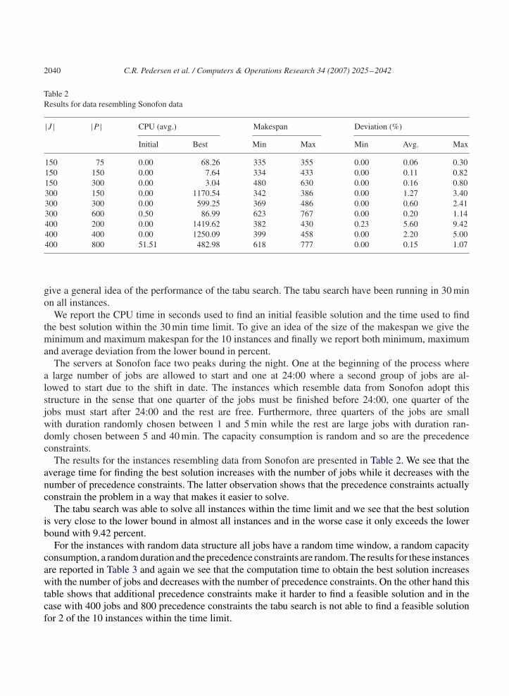
Table 2Results for data resembling Sonofon data
|J | |P | CPU (avg.) Makespan Deviation (%)
Initial Best Min Max Min Avg. Max
150 75 0.00 68.26 335 355 0.00 0.06 0.30150 150 0.00 7.64 334 433 0.00 0.11 0.82150 300 0.00 3.04 480 630 0.00 0.16 0.80300 150 0.00 1170.54 342 386 0.00 1.27 3.40300 300 0.00 599.25 369 486 0.00 0.60 2.41300 600 0.50 86.99 623 767 0.00 0.20 1.14400 200 0.00 1419.62 382 430 0.23 5.60 9.42400 400 0.00 1250.09 399 458 0.00 2.20 5.00400 800 51.51 482.98 618 777 0.00 0.15 1.07
give a general idea of the performance of the tabu search. The tabu search have been running in 30 minon all instances.
We report the CPU time in seconds used to find an initial feasible solution and the time used to findthe best solution within the 30 min time limit. To give an idea of the size of the makespan we give theminimum and maximum makespan for the 10 instances and finally we report both minimum, maximumand average deviation from the lower bound in percent.
The servers at Sonofon face two peaks during the night. One at the beginning of the process wherea large number of jobs are allowed to start and one at 24:00 where a second group of jobs are al-lowed to start due to the shift in date. The instances which resemble data from Sonofon adopt thisstructure in the sense that one quarter of the jobs must be finished before 24:00, one quarter of thejobs must start after 24:00 and the rest are free. Furthermore, three quarters of the jobs are smallwith duration randomly chosen between 1 and 5 min while the rest are large jobs with duration ran-domly chosen between 5 and 40 min. The capacity consumption is random and so are the precedenceconstraints.
The results for the instances resembling data from Sonofon are presented in Table 2. We see that theaverage time for finding the best solution increases with the number of jobs while it decreases with thenumber of precedence constraints. The latter observation shows that the precedence constraints actuallyconstrain the problem in a way that makes it easier to solve.
The tabu search was able to solve all instances within the time limit and we see that the best solutionis very close to the lower bound in almost all instances and in the worse case it only exceeds the lowerbound with 9.42 percent.
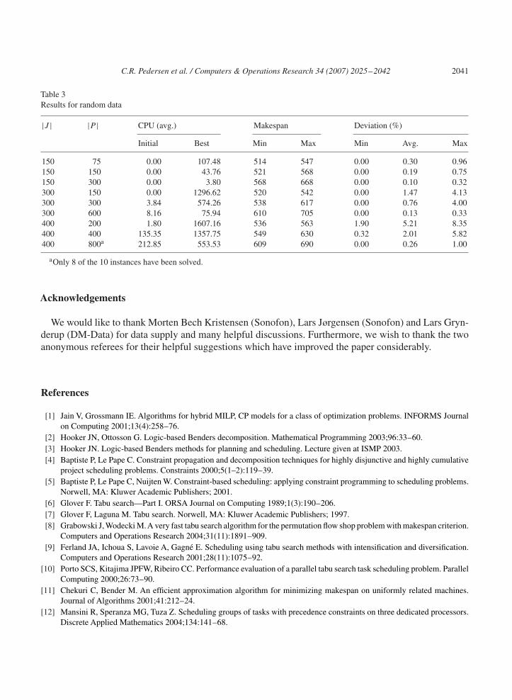
For the instances with random data structure all jobs have a random time window, a random capacityconsumption, a random duration and the precedence constraints are random. The results for these instancesare reported in Table 3 and again we see that the computation time to obtain the best solution increaseswith the number of jobs and decreases with the number of precedence constraints. On the other hand thistable shows that additional precedence constraints make it harder to find a feasible solution and in thecase with 400 jobs and 800 precedence constraints the tabu search is not able to find a feasible solutionfor 2 of the 10 instances within the time limit.
C.R. Pedersen et al. / Computers & Operations Research 34 (2007) 2025–2042 2041
Table 3Results for random data
|J | |P | CPU (avg.) Makespan Deviation (%)
Initial Best Min Max Min Avg. Max
150 75 0.00 107.48 514 547 0.00 0.30 0.96150 150 0.00 43.76 521 568 0.00 0.19 0.75150 300 0.00 3.80 568 668 0.00 0.10 0.32300 150 0.00 1296.62 520 542 0.00 1.47 4.13300 300 3.84 574.26 538 617 0.00 0.76 4.00300 600 8.16 75.94 610 705 0.00 0.13 0.33400 200 1.80 1607.16 536 563 1.90 5.21 8.35400 400 135.35 1357.75 549 630 0.32 2.01 5.82400 800a 212.85 553.53 609 690 0.00 0.26 1.00
aOnly 8 of the 10 instances have been solved.
Acknowledgements
We would like to thank Morten Bech Kristensen (Sonofon), Lars JZrgensen (Sonofon) and Lars Gryn-derup (DM-Data) for data supply and many helpful discussions. Furthermore, we wish to thank the twoanonymous referees for their helpful suggestions which have improved the paper considerably.
References
[1] Jain V, Grossmann IE. Algorithms for hybrid MILP, CP models for a class of optimization problems. INFORMS Journalon Computing 2001;13(4):258–76.
[2] Hooker JN, Ottosson G. Logic-based Benders decomposition. Mathematical Programming 2003;96:33–60.[3] Hooker JN. Logic-based Benders methods for planning and scheduling. Lecture given at ISMP 2003.[4] Baptiste P, Le Pape C. Constraint propagation and decomposition techniques for highly disjunctive and highly cumulative
project scheduling problems. Constraints 2000;5(1–2):119–39.[5] Baptiste P, Le Pape C, Nuijten W. Constraint-based scheduling: applying constraint programming to scheduling problems.
Norwell, MA: Kluwer Academic Publishers; 2001.[6] Glover F. Tabu search—Part I. ORSA Journal on Computing 1989;1(3):190–206.[7] Glover F, Laguna M. Tabu search. Norwell, MA: Kluwer Academic Publishers; 1997.[8] Grabowski J, Wodecki M.A very fast tabu search algorithm for the permutation flow shop problem with makespan criterion.
Computers and Operations Research 2004;31(11):1891–909.[9] Ferland JA, Ichoua S, Lavoie A, Gagné E. Scheduling using tabu search methods with intensification and diversification.
Computers and Operations Research 2001;28(11):1075–92.[10] Porto SCS, Kitajima JPFW, Ribeiro CC. Performance evaluation of a parallel tabu search task scheduling problem. Parallel
Computing 2000;26:73–90.[11] Chekuri C, Bender M. An efficient approximation algorithm for minimizing makespan on uniformly related machines.
Journal of Algorithms 2001;41:212–24.[12] Mansini R, Speranza MG, Tuza Z. Scheduling groups of tasks with precedence constraints on three dedicated processors.
Discrete Applied Mathematics 2004;134:141–68.

2042 C.R. Pedersen et al. / Computers & Operations Research 34 (2007) 2025–2042
[13] Chiang W-C, Russell RA. A reactive tabu search metaheuristic for the vehicle routing problem with time windows.INFORMS Journal on Computing 1997;9(4):417–30.
[14] Garey MR, Johnson DS. Computers and intractability. a guide to the theory of NP-completeness. NewYork: W.H. Freemanand Company; 1979.
[15] ILOG, ILOG Optimization Suite—white paper 2001. http://www.ilog.com.