solution of single and multiobjective stochastic inventory...

Hindawi Publishing CorporationAdvances in Operations ResearchVolume 2010, Article ID 765278, 19 pagesdoi:10.1155/2010/765278

Research ArticleSolution of Single and Multiobjective StochasticInventory Models with Fuzzy Cost Components byIntuitionistic Fuzzy Optimization Technique

S. Banerjee and T. K. Roy

Department of Mathematics, Bengal Engineering and Science University, Shibpur, Howrah 711103, India

Correspondence should be addressed to S. Banerjee, sou [email protected]

Received 14 August 2009; Revised 26 January 2010; Accepted 5 March 2010

Academic Editor: Ching Jong Liao

Copyright q 2010 S. Banerjee and T. K. Roy. This is an open access article distributed underthe Creative Commons Attribution License, which permits unrestricted use, distribution, andreproduction in any medium, provided the original work is properly cited.

Paknejad et al.’s model is considered in this paper. Itemwise multiobjective models for bothexponential and uniform lead-time demand are taken and the results are compared numericallyboth in fuzzy optimization and intuitionistic fuzzy optimization techniques. Objective of thispaper is to establish that intuitionistic fuzzy optimizaion method is better than usual fuzzyoptimization technique as expected annual cost of this inventory model is more minimized incase of intuitionistic fuzzy optimization method. As a single objective stochastic inventory modelwhere the lead-time demand follows normal distribution and with varying defective rate, expectedannual cost is also measured. Finally the model considers for fuzzy cost components, whichmake the model more realistic, and numerical values for uniform, exponential, and normal lead-time demand are compared. Necessary graphical presentations are also given besides numericalillustrations.

1. Introduction

In conventional inventory models, uncertainties are treated as randomness and are handledby appealing to probability theory. However, in certain situations uncertainties are dueto fuzziness and in these cases the fuzzy set theory, originally introduced by Zadeh[1], is applicable. Today most of the real-world decision-making problems in economic,technical and environmental ones are multidimensional and multiobjective. It is significantto realize that multiple-objectives are often noncommensurable and conflict with each otherin optimization problem. An objective within exact target value is termed as fuzzy goal. So amultiobjective model with fuzzy objectives is more realistic than deterministic of it.

In decision making process, first, Bellman and Zadeh [2] introduced fuzzy set theory;Tanaka et al. [3] applied concept of fuzzy sets to decision-making problems to consider theobjectives as fuzzy goals over the α-cuts of a fuzzy constraints. Zimmermann [4, 5] showed

2 Advances in Operations Research

that the classical algorithms can be used in few inventory models. Li et al. [6] discussedfuzzy models for single-period inventory problem in 2002. Abou-El-Ata et al. [7] consideredin 2003 a probabilistic multiitem inventory model with varying order cost. A single-periodinventory model with fuzzy demand is analyzed by Kao and Hsu [8]. Fergany and El-Wakeel[9] considered a probabilistic single-item inventory problem with varying order cost undertwo linear constraints. A survey of literature on continuously deteriorating inventory modelsare discussed by Raafat [10]. Hala and EI-Saadani [11] analyzed a constrained single periodstochastic uniform inventory model with continuous distributions of demand and varyingholding cost. Some inventory problems with fuzzy shortage cost is discussed by Katagiriand Ishii [12]. Moon and Choi [13] implemented a note on lead time and distributionalassumptions in continuous review inventory models. Lai and Hwang [14, 15] elaboratelydiscussed fuzzy mathematical programming and fuzzy multiple objective decision making intheir two renowned contributions. Ouyang and Chang [16] analyzed a minimax distributionfree procedure for mixed inventory models involving variable lead time with fuzzy lostsales. Mahapatra and Roy [17] discussed fuzzy multiobjective mathematical programmingon reliability optimization model. Hariga and Ben-Daya [18] considered some stochasticinventory models with deterministic variable lead time. A fuzzy EOQ model with demand-dependent unit cost under limited storage capacity is implemented by Roy and Maiti [19].Zheng [20] discussed optimal control policy for stochastic inventory systems with Markoviandiscount opportunities.

Intuitionistic Fuzzy Set (IFS) was introduced by Atanassov [21] and seems to beapplicable to real world problems. The concept of IFS can be viewed as an alternativeapproach to define a fuzzy set in case where available information is not sufficient for thedefinition of an imprecise concept by means of a conventional fuzzy set. Thus it is expectedthat IFS can be used to simulate human decision-making process and any activitities requiringhuman expertise and knowledge that are inevitably imprecise or totally reliable. Here thedegrees of rejection and satisfaction are considered so that the sum of both values is alwaysless than unity [21]. Atanassov also analyzed Intuitionistic fuzzy sets in a more explicitway. Atanassov and Gargov [22] discussed an Open problem in intuitionistic fuzzy setstheory. An Interval-valued intuitionistic fuzzy set was analyzed byAtanassov [23]. Atanassovand Kreinovich [24] implemented Intuitionistic fuzzy interpretation of interval data. Thetemporal intuitionistic fuzzy sets are discussed also by Atanassov [25]. Intuitionistic fuzzysoft sets are considered by Maji et al. [26]. Nikolova et al. [27] presented a Survey of theresearch on intuitionistic fuzzy sets. Rough intuitionistic fuzzy sets are analyzed by Rizvi etal. [28]. Angelov [29] implemented the Optimization in an intuitionistic fuzzy environment.He [30, 31] also contributed in another two important papers, based on Intuitionisticfuzzy optimization. Pramanik and Roy [32] solved a vector optimization problem using anIntuitionistic Fuzzy goal programming. A transportation model is solved by Jana and Roy[33] using multi-objective intuitionistic fuzzy linear programming.

Paknejad et al.[35] presented a quality adjusted lot-sizing model with stochasticdemand and constant lead time and studied the benefits of lower setup cost in the model.We note that the previous literature focuses on the issue of setup cost reduction in whichinformation about lead-time demand, whether constant or stochastic, is assumed completelyknown. Ouyang and Chang [34] modified Paknejad et al.’s inventory model by relaxingthe assumption that the stochastic demand during lead time follows a specific probabilitydistribution and by considering that the unsatisfied demands are partially backordered.Also, instead of having a stockout cost in the objective function, a service level constraintis employed.

Advances in Operations Research 3

Paknejad et al.’s [35] model is considered in this paper, as a single objective stochasticinventory model where the lead-time demand follows normal distribution and with varyingdefective rate, expected annual cost is measured. Itemwise multiobjective models forboth exponential and uniform lead time demand are taken and the results are comparednumerically both in fuzzy optimization and intuitionistic fuzzy optimization techniques.From our numerical as well as graphical presentations, it is clear that intuitionistic fuzzyoptimization obtains better results than fuzzy optimization. Finally the model considers forseveral fuzzy costs and numerical values for uniform, exponential, and normal lead-timedemand are compared. Necessary graphical presentations are also given besides numericalillustrations.

2. Mathematical Model

Paknejad et al. [35] presented a quality adjusted lot-sizing model with stochastic demand andconstant lead time and studied the benefits of lower setup cost in the model. We note that theprevious literature focuses on the issue of setup cost reduction in which information aboutlead-time demand, whether constant or stochastic, is assumed completely known. This paperconsiders Paknejad et al.’s model along with the notations and some assumptions that willbe taken into account throughout the paper. Each lot contains a random number of defectivesfollowing binomial distribution. After the arrival purchaser examines the entire lot, an orderof sizeQ is placed as soon as the inventory position reaches the reorder point s. The shortagesare allowed and completely backordered. Lead-time is constant and probability distributionof lead-time demand is known.

Now, we use the following notations:

D: expected demand per year,

Q: lot size,

s: reorder point,

K: setup cost,

θ: defective rate in a lot of size Q, 0 ≤ θ ≤ 1,

h: nondefective holding cost per unit per year,

h′: defective holding cost per unit per year,

π : shortage cost per unit short,

ν: cost of inspecting a single item in each lot,

μ: expected demand during lead time,

b(s): the expected demand short at the end of the cycle

b(s) =∫∞s

(x − s)f(x)dx, (2.1)

where f(x) is the density function of lead-time demand,

EC(Q, s): expected annual cost given that a lot size Q is ordered.


3. Single Objective Stochastic Inventory Model (SOSIM)

Thus a quality-adjusted lot-sizing model is formed as

MinEC(Q, s) = Setup cost + non-defective item holding cost + stockout cost

+ defective item holding cost + inspecting cost

=DK

Q(1 − θ) + h(s − μ +

12(Q(1 − θ) + θ)

)

+Dπb(s)Q(1 − θ) + h

′θ(Q − 1) +Dv

1 − θ Q, s > 0.

(3.1)

It is the stochastic model, which minimizes the expected annual cost.

4. Multiobjective Stochastic Inventory Model (MOSIM)

In reality, a managerial problem of a responsible organization involves several conflictingobjectives to be achieved simultaneously that refers to a situation on which the DM hasno control. For this purpose a latest tool is linear or nonlinear programming problem withmultiple conflicting objectives. So the following model may be considered.

To solve the problem in (3.1) as an MOSIM, it can be reformulated as

MinECi(Qi, si)=DiKi

Qi(1 − θi)+hi(si − μi +

12(Qi(1 − θi)+θi)

)

+Diπbi(si)Qi(1 − θi)

+ h′iθi(Qi − 1)+Divi1 − θi

Qi, si > 0 ∀i = 1, 2, . . . , n.

(4.1)

5. Multiitem Stochastic Model with Fuzzy Cost Components

Stochastic nonlinear programming problem with fuzzy cost components considers as

MinEC(Q1, . . . , Qn, s1, . . . , sn)

=n∑i=1

(DiK̃i

Qi(1 − θi)+h̃i(si−μi+

12(Qi(1−θi)+θi)

)+Diπ̃ibi(s)Qi(1−θi)

+h̃′iθi(Qi − 1)+Divi1 − θi

)

Qi, si > 0 ∀i = 1, 2, . . . , n.(5.1)

Here K̃i, π̃i, h̃i, h̃′i represent vector of fuzzy parameters involved in the objective function

EC. We assume K̃i = (K−i , K0i , K

+i ), π̃i = (π−i , π

0i , π

+i ), h̃i = (h−i , h

0i , h

+i ), and h̃′i = (h′−i , h

′0i , h

′+i ),

all of which are triangular fuzzy numbers.


6. Fuzzy Nonlinear Programming (FNLP) Technique toSolve Multiobjective Nonlinear Programming Problem (MONLP)

A Multi-Objective Non-Linear Programming (MONLP) or Vector Minimization problem(VMP) may be taken in the following form:

M inf(x) =(f1(x), f2(x), . . . , fk(x)

)TSubject to x ∈ X =

{x ∈ Rn : gj(x) ≤ or = or ≥ bj for j = 1, 2, . . . , m

}li ≤ x ≤ ui (i = 1, 2, . . . , n).

(6.1)

Zimmermann [5] showed that fuzzy programming technique can be used to solve the multi-objective programming problem.

To solve MONLP problem, the following steps are used.

Step 1. Solve the MONLP of (6.1) as a single objective non-linear programming problemusing only one objective at a time and ignoring the others; these solutions are known as idealsolution.

Step 2. From the result of Step 1, determine the corresponding values for every objective ateach solution derived. With the values of all objectives at each ideal solution, pay-off matrixcan be formulated as follows:

f1(x) f2(x) . . . fk(x)x1

x2

. . .xk

⎡⎢⎢⎣f∗1(x1)

f1(x2). . .

f1(xk)

f2(x1)

f∗2(x2). . .

f2(xk)

. . .

. . .

. . .

. . .

fk(x1)

fk(x2). . .

f∗k

(xk)

⎤⎥⎥⎦. (6.2)

Here x1, x2, . . . , xk are the ideal solutions of the objective functions f1(x), f2(x), . . . , fk(x),respectively.

So

Ur = max{fr(x1), fr(x2), . . . , fr(xk)

},

Lr = min{fr(x1), fr(x2), . . . , fr(xk)

} (6.3)

(Lr and Ur are lower and upper bounds of the rth objective functions fr(x) r = 1, 2, . . . , k)).

Step 3. Using aspiration level of each objective of the MONLP of (6.1) may be written asfollows.

Find x so as to satisfy

fr(x)≤̃Lr (r = 1, 2, . . . , k), x ∈ X. (6.4)


Here objective functions of (6.1) are considered as fuzzy constraints. These type offuzzy constraints can be quantified by eliciting a corresponding membership function:

μr(fr(x)

)=

⎧⎪⎪⎪⎨⎪⎪⎪⎩

0 or −→ 0 if fr(x) ≥ Ur

μr(fr(x)

)if Lr ≤ fr(x) ≤ Ur (r = 1, 2, . . . , k)

1 if fr(x) ≤ Lr.

(6.5)

Having elicited the membership functions (as in (6.5)) μr(fr(x)) for r = 1, 2, . . . , k introducea general aggregation function:

μD̃(x) = G(μ1(f1(x)

), μ2(f2(x)

), . . . , μk

(fk(x)

)). (6.6)

So a fuzzy multi-objective decision making problem can be defined as

Max μD̃(x)

subject to x ∈ X.(6.7)

Here we adopt the fuzzy decision as follows.Fuzzy decision is based on minimum operator (like Zimmermann’s approach [4]). In

this case (6.7) is known as FNLPM.Then the problem of (6.7), using the membership function as in (6.5), according to

min-operator is reduced to

Max α

Subject to μi(fi(x)

)≥ α for (i = 1, 2, . . . , k), x ∈ X α ∈ [0, 1].

(6.8)

Step 4. Solve (6.8) to get optimal solution.

7. Stochastic Models with Fuzzy Cost Components

Stochastic non-linear programming problem with fuzzy objective coefficient considers as

MinZ = C̃X, X ≥ 0. (7.1)


Here C̃ represents a vector of fuzzy parameters involved in the objective function Z. Weassume C̃i= (ci−, ci0, ci+), which is a triangular fuzzy number with membership function:

μC̃i(t) =

⎧⎪⎪⎪⎪⎪⎪⎪⎪⎪⎪⎪⎨⎪⎪⎪⎪⎪⎪⎪⎪⎪⎪⎪⎩

t − c−ici0 − c−i

for c−i ≤ t ≤ c0i ,

c+i − tc+i − c

0i

for c0i ≤ t ≤ c

+i ,

0 for t > c+i or t < c−i .

(7.2)

So (7.1) becomes

MinZ =(c−i X, c

0i X, c

+i X), X ≥ 0, (7.3)

where

c− =(c−1 , c

−2 , . . . , c

−n

),

c0 =(c0

1, c02, . . . , c

0n

),

c+ =(c+1 , c

−2 , . . . , c

+n

).

(7.4)

According to Kaufman and Gupta [36] by combining three objectives into a single objectivefunction, (7.3) can be reduced to an LPP by most likely criteria as

Min

(c− + 4c0 + c+

6

)X, X ≥ 0. (7.5)

8. Formulation of Intuitionistic Fuzzy Optimization

When the degree of rejection (nonmembership) is defined simultaneously with degreeof acceptance (membership) of the objectives and when both of these degrees are notcomplementary to each other, then IF sets can be used as a more general tool for describinguncertainty.


(μk, vk)

μk(Zk(X))

vk(Zk(X))

Zk(X)Uacck

= Urejk

Lacck

Lrejk

1 1

Figure 1: Membership and nonmemebership functions of the objective goal.

To maximize the degree of acceptance of IF objectives and constraints and to minimizethe degree of rejection of IF objectives and constraints, we can write

max μi(X), XεR, i = 1, 2, . . . , K + n,

min υi(X), XεR, i = 1, 2, . . . , K + n,

Subject to υi(X)≥ 0,

μi(X)≥ υi(X),

μi(X)+ υi(X)< 1,

X ≥ 0,

(8.1)

where μi(X) denotes the degree of membership function of (X) to the ith IF sets and νi(X)denotes the degree of nonmembership (rejection) of (X) from the ith IF sets.

9. An Intuitionistic Fuzzy Approach for Solving MOIP with LinearMembership and Nonmembership Functions

To define the membership function of MOIM problem, let Lacck

and Uacck

be the lower andupper bounds of the kth objective function. These values are determined as follows. Calculatethe individual minimum value of each objective function as a single objective IP subject tothe given set of constraints. Let X

∗1, X

∗2, . . . , X

∗k be the respective optimal solution for the k

different objective and evaluate each objective function at all these k optimal solutions. It isassumed here that at least two of these solutions are different for which the kth objective func-tion has different bounded values. For each objective, find lower bound (minimum value)Lacck and the upper bound (maximum value) Uacc

k . But in intuitionistic fuzzy optimization(IFO), the degree of rejection (non-membership) and degree of acceptance (membership) areconsidered so that the sum of both values is less than one. To define membership functionof MOIM problem, let Lrej

k and Urejk be the lower and upper bounds of the objective function

Zk(X) where Lacck≤ Lrej

k≤ Urej

k≤ Uacc

k. These values are defined as follows.


The linear membership function for the objective Zk(X) is defined as

μk(Zk

(X))

=

⎧⎪⎪⎪⎪⎪⎪⎨⎪⎪⎪⎪⎪⎪⎩

1 if Zk

(X)≤ Lacc

k ,

Uacck − Zk

(X)

Uacck− Lacc

k

if Lacck ≤ Zk

(X)≤ Uacc

k ,

0 if Zk

(X)≥ Uacc

k,

νk(Zk

(X))

=

⎧⎪⎪⎪⎪⎪⎪⎨⎪⎪⎪⎪⎪⎪⎩

1 if Zk

(X)≥ Urej

k,

Zk

(X)− Lrej

k

Urejk− Lrej

k

if Lrejk≤ Zk

(X)≤ Urej

k,

0 if Zk

(X)≤ Lrej

k .

(9.1)

Lemma 9.1. In case of minimization problem, the lower bound for non-membership function(rejection) is always greater than that of the membership function (acceptance).

Now, we take new lower and upper bounds for the non-membership function asfollows:

Lrejk

= Lacck + t

(Uacck − L

acck

), where 0 < t < 1,

Urejk = Uacc

k + t(Uacck − L

acck

)for t = 0.

(9.2)

Following the fuzzy decision of Bellman-Zadeh [2] together with linear membershipfunction and non-membership functions of (9.1), an intuitionistic fuzzy optimization modelof MOIM problem can be written as

max μk(X), XεR, k = 1, 2, . . . , K,

min υk(X), XεR, k = 1, 2, . . . , K

Subject to υk(X)≥ 0,

μk(X)≥ υk

(X),

μk(X)+ υk

(X)< 1,

X ≥ 0.

(9.3)


The problem of (9.3) can be reduced following Angelov [29] to the following form:

Max α − β

Subject to Zk

(X)≤ Uacc

k − α(Uacck − L

acck

),

Zk

(X)≤ Lrej

k+ β(U

rejk− Lrej

k

),

β ≥ 0,

α ≥ β,

α + β < 1,

X ≥ 0,

(9.4)

Then the solution of the MOIM problem is summarized in the following steps.

Step 1. Pick the first objective function and solve it as a single objective IP subject to theconstraint; continue the processK-times forK different objective functions. If all the solutions(i.e., X

∗1 = X

∗2 = · · · = X

∗k (i = 1, 2, . . . , m; j = 1, 2, . . . , n)) are the same, then one of them is the

optimal compromise solution and go to Step 6. Otherwise go to Step 2. However, this rarelyhappens due to the conflicting objective functions.

Then the intuitionistic fuzzy goals take the form

Zk

(X)≤̃ Lk

(X)∗k

k = 1, 2, . . . , K. (9.5)

Step 2. To build membership function, goals and tolerances should be determined at first.Using the ideal solutions, obtained in Step 1, we find the values of all the objective functionsat each ideal solution and construct pay off matrix as follows:

⎡⎢⎢⎢⎢⎢⎢⎢⎢⎢⎢⎢⎢⎢⎢⎢⎣

Z1

(X∗1

)Z2

(X∗1

)· · · · · · · · · Zk

(X∗1

)

Z1

(X∗2

)Z2

(X∗2

)· · · · · · · · · Zk

(X∗2

)

· · · · · · · · · · · · · · · · · ·

· · · · · · · · · · · · · · · · · ·

· · · · · · · · · · · · · · · · · ·

Z1

(X∗k

)Z2

(X∗k

)· · · · · · · · · Zk

(X∗k

)

⎤⎥⎥⎥⎥⎥⎥⎥⎥⎥⎥⎥⎥⎥⎥⎥⎦

. (9.6)

Step 3. From Step 2, we find the upper and lower bounds of each objective for the degree ofacceptance and rejection corresponding to the set of solutions as follows:

Uacck = max

(Zk

(X∗r

)), Lacc

k = min(Zk

(X∗r

)), 1 ≤ r ≤ k. (9.7)


For linear membership functions,

Lrejk

= Lacck + t

(Uacck − L

acck

), where 0 < t < 1,

Urejk

= Uacck + t

(Uacck − L

acck

)for t = 0.

(9.8)

Step 4. Construct the fuzzy programming problem of (9.3) and find its equivalent LP problemof (9.4).

Step 5. Solve (9.4) by using appropriate mathematical programming algorithm to get anoptimal solution and evaluate the K objective functions at these optimal compromisesolutions.

Step 6. STOP.

10. Few Stochastic Models

Case 1 (Demand follows Uniform distribution). We assume that lead time demand for theperiod for the ith item is a random variable which follows uniform distribution and if thedecision maker feels that demand values for item I below ai or above bi are highly unlikelyand values between ai and bi are equally likely, then the probability density function fi(x) isgiven by

fi(x) =

⎧⎪⎨⎪⎩

1bi − ai

, if ai ≤ x ≤ bi,

0, otherwise,for i = 1, 2, . . . , n. (10.1)

So,

bi(si) =(bi − si)2

2(bi − ai)for i = 1, 2, . . . , n, (10.2)

where bi(si) are the expected number of shortages per cycle and all these values of bi(si) affectall the desired models.

Case 2 (Demand follows Exponential distribution). We assume that lead-time demand for theperiod for the ith item is a random variable that follows exponential distribution. Then theprobability density function fi(x) is given by

fi(x) =

{λie

(−λix), x > 0 for i = 1, 2, . . . , n,0, otherwise.

(10.3)

So,

bi(si) =e−λisi

(−λi)for i = 1, 2, . . . , n, (10.4)


where bi(si) are the expected number of shortages per cycle and all these values of bi(si) affectall the desired models.

Case 3 (Demand follows Normal distribution). We assume that lead-time demand for theperiod for the ith item is a random variable, which follows normal distribution. Then theprobability density function fi(x) is given by

fi(x) =1

σi√

2πexp

(−(x − μi

)2

2σi2

), −∞ < x <∞,

bi(si) =

(μi − si

)σi√

2π

(1 −Φ

(si − μiσi

))+

1√2π

exp

(−(μi − si

)2

2σi2

)for i = 1, 2, . . . , n,

(10.5)

where bi(si) are the expected number of shortages per cycle and all these values of bi(si)affects all the desired models and Φ(xi) represents area under standard normal curve from−∞ to xi.

11. Numericals

11.1. Solution of the Model of (3.1)

The lead-time demand follows normal distribution and thus bi(si), the expected demandshort at the end of the cycle, takes up the value according to (10.2). Thus for single itemmodel, we consider the following data:

D = 2750; K = 10; h = 0.25; v = 0.02; π = 1; h′ = 0.15 (11.1)

(all the cost-related parameters are measured in “$”).Here, the lead-time demand follows Normal distribution with mean μ = 20 and

standard deviation σ = 2.The lead-time demand follows normal distribution and thus bi(si), the expected

demand short at the end of the cycle, takes up the value according to (10.2).In Table 1, a study of expected annual cost EC(Q, s) with lot size Q and reorder point

s is given for different defective rate θ. We conclude from Table 1 as well asFigure 2 that theorder quantity as well as the expected annual cost increases as θ increases.


In case of MOSIM of (4.1), we use the methods described in Section 6, to solve it by fuzzyoptimization technique, and Sections 8 and 9, to solve it by intuitionistic fuzzy optimizationtechnique and the following data are considered.


0

200

400

600

800

1000

1200

1400

θ

EC∗(Q, s)Q∗

1

0.1186.347489.248

2

0.2202.854513.793

3

0.3223.274543.933

4

0.4249.389581.908

5

0.5284.312631.468

6

0.6334.073699.485

7

0.7412.221800.352

8

0.8557.593971.432

9

0.9952.6871361.61

Figure 2

Table 1: Variation of “EC” and “s” with “θ”.

θ EC∗ ($) Q∗

0.1 186.3471 489.24840.2 202.8538 513.79290.3 223.2740 543.93290.4 249.3887 581.90800.5 284.3121 631.46770.6 334.0731 699.48500.7 412.2208 800.35150.8 557.5926 971.43240.9 952.6872 1361.609

Case 1. The lead-time demand follows uniform distribution and thus bi(si), the expecteddemand short at the end of the cycle, takes up the value according to (10.2).

We consider two different sets of data as

D1 = 2700; K1 = 12; h1 = 0.55; θ1 = 0.6; μ1 =(a1 + b1)

2;

ν1 = 0.03; π1 = 1; h′1 = 0.25; a1 = 20; b1 = 70; μ1 =(a1 + b1)

2.

D2 = 2750; K2 = 10; h2 = 0.25; θ2 = 0.8; μ2 =(a2 + b2)

2; ν2 = 0.02;

π2 = 2; h′2 = 0.15; a2 = 10; b2 = 50; μ2 =(a2 + b2)

2.

(11.2)


Table 2: Comparison of solutions of FO and IFO (UNIFORM).

Methods Q1 Q2 s1 S2 EC1($) EC2($) α∗ β∗Fuzzyoptimization

415.3 1042.3 69.157 44.778 519.0996 570.8203 0.9599 —

IntuitionisticFuzzyoptimization

967.6 1136.8 65.371 49.647 516.8335 563.7091 0.76 0.023

The pay-off matrix is

EC1 EC2

[506.0453 804.4216

831.6330 562.4362

] (11.3)

We take

Uacc1 = 831.6330; Lacc

1 = 506.0453; Uacc2 = 804.4216; Lacc

2 = 562.4362;

Urej1 = 831.6330; L

rej1 = 507; U

rej2 = 804.4216; L

rej2 = 570

(11.4)

(all the cost -related parameters are measured in “$”).Then from Table 2 andFigure 3 we conclude that Intuitionistic fuzzy optimization

(IFO) obtains more optimized values of EC1 and EC2 than fuzzy optimization (FO). Alsosolution obtained by IFO (516.8335, 563.7091) is closer to the ideal solution (506.0453,562.4362) than the solution obtained by FO.

Case 2. The lead-time demand follows exponential distribution and thus bi(si), the expecteddemand short at the end of the cycle, takes up the value according to (10.4).

We consider two different sets of data as

D1 = 2700; K1 = 8; h1 = 1; θ1 = 0.4; μ1 =1λ1

; ν1 = 0.03;

π1 = 1; h′1 = 0.25; λ1 = 1;

D2 = 2750; K2 = 10; h2 = 1; θ2 = 0.7; ν2 = 0.02; π2 = 1.1;

h′2 = 0.15; μ2 =1λ2

; λ2 = 1.1.

(11.5)

The pay-off matrix is

EC1 EC2

[378.0060 523.5858

551.0537 382.4234

] (11.6)


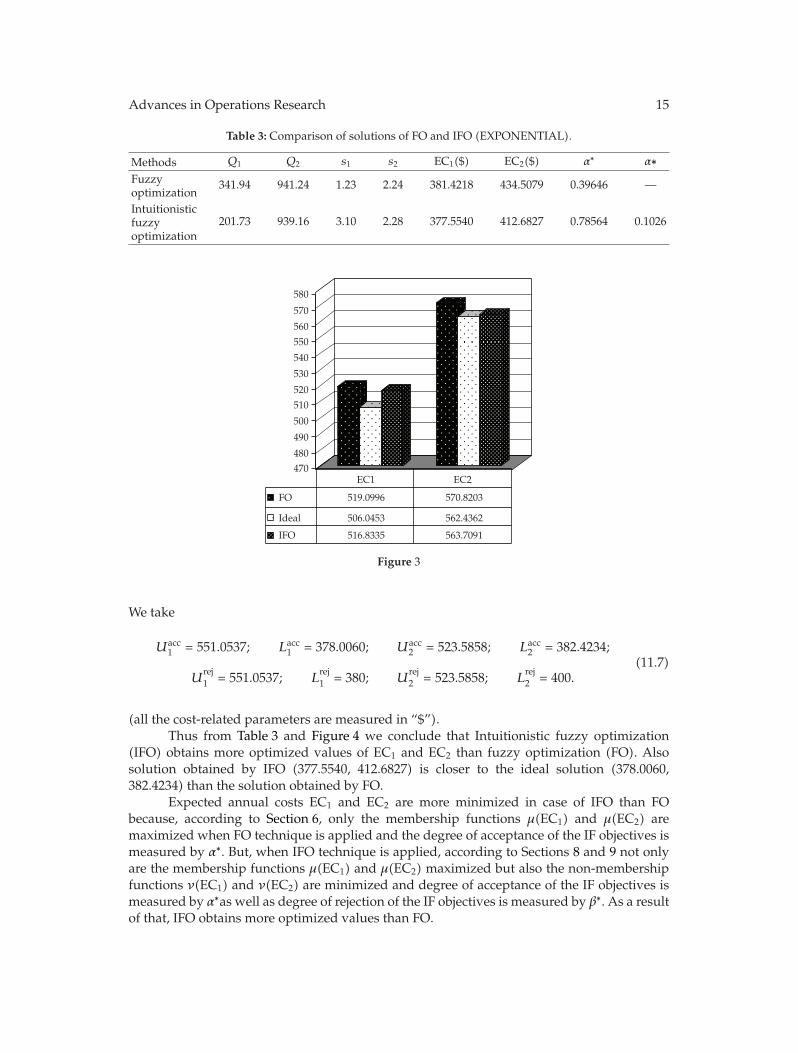
Table 3: Comparison of solutions of FO and IFO (EXPONENTIAL).

Methods Q1 Q2 s1 s2 EC1($) EC2($) α∗ α∗Fuzzyoptimization

341.94 941.24 1.23 2.24 381.4218 434.5079 0.39646 —

Intuitionisticfuzzyoptimization

201.73 939.16 3.10 2.28 377.5540 412.6827 0.78564 0.1026

470

480

490

500

510

520

530

540

550

560

570

580

FO

Ideal

IFO

EC1

519.0996

506.0453

516.8335

EC2

570.8203

562.4362

563.7091

Figure 3

We take

Uacc1 = 551.0537; Lacc

1 = 378.0060; Uacc2 = 523.5858; Lacc

2 = 382.4234;

Urej1 = 551.0537; L

rej1 = 380; U

rej2 = 523.5858; L

rej2 = 400.

(11.7)

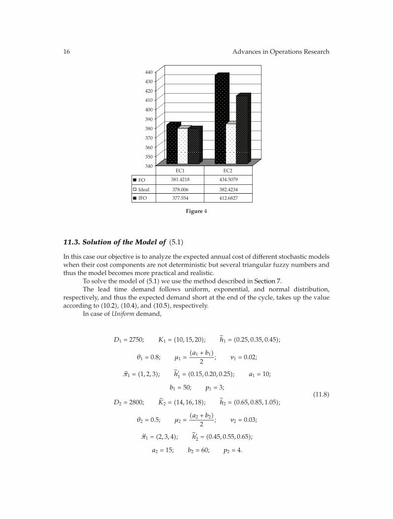
(all the cost-related parameters are measured in “$”).Thus from Table 3 and Figure 4 we conclude that Intuitionistic fuzzy optimization

(IFO) obtains more optimized values of EC1 and EC2 than fuzzy optimization (FO). Alsosolution obtained by IFO (377.5540, 412.6827) is closer to the ideal solution (378.0060,382.4234) than the solution obtained by FO.

Expected annual costs EC1 and EC2 are more minimized in case of IFO than FObecause, according to Section 6, only the membership functions μ(EC1) and μ(EC2) aremaximized when FO technique is applied and the degree of acceptance of the IF objectives ismeasured by α∗. But, when IFO technique is applied, according to Sections 8 and 9 not onlyare the membership functions μ(EC1) and μ(EC2) maximized but also the non-membershipfunctions ν(EC1) and ν(EC2) are minimized and degree of acceptance of the IF objectives ismeasured by α∗as well as degree of rejection of the IF objectives is measured by β∗. As a resultof that, IFO obtains more optimized values than FO.


340

350

360

370

380

390

400

410

420

430

440

FO

Ideal

IFO

EC1

381.4218

378.006

377.554

EC2

434.5079

382.4234

412.6827

Figure 4


In this case our objective is to analyze the expected annual cost of different stochastic modelswhen their cost components are not deterministic but several triangular fuzzy numbers andthus the model becomes more practical and realistic.

To solve the model of (5.1) we use the method described in Section 7.The lead time demand follows uniform, exponential, and normal distribution,

respectively, and thus the expected demand short at the end of the cycle, takes up the valueaccording to (10.2), (10.4), and (10.5), respectively.

In case of Uniform demand,

D1 = 2750; K1 = (10, 15, 20); h̃1 = (0.25, 0.35, 0.45);

θ1 = 0.8; μ1 =(a1 + b1)

2; ν1 = 0.02;

π̃1 = (1, 2, 3); h̃′1 = (0.15, 0.20, 0.25); a1 = 10;

b1 = 50; p1 = 3;

D2 = 2800; K̃2 = (14, 16, 18); h̃2 = (0.65, 0.85, 1.05);

θ2 = 0.5; μ2 =(a2 + b2)

2; ν2 = 0.03;

π̃1 = (2, 3, 4); h̃′2 = (0.45, 0.55, 0.65);

a2 = 15; b2 = 60; p2 = 4.

(11.8)


Table 4: Expected Annual costs of different stochastic models.

Prob. distribution EC ($) Q1 Q2 s1 s2

UNIFORM 1459.05 491.64 256.26 49.74 59.41EXPONENTIAL 1260.15 502.27 750.00 2.9 3.01NORMAL 831.05 335.5 305.79 20.86 10.55

In case of Exponential demand,

D1 = 2750; K̃1 = (10, 12, 14); h̃1 = (1, 2, 3); θ1 = 0.7; λ1 = 1;

ν1 = 0.02; π̃1 = (1, 2, 3); h̃′1 = (0.15, 0.20, 0.25); p1 = 4;

D2 = 2700; K̃2 = (8, 10, 12); h̃2 = (0.6, 0.8, 1); θ2 = 0.8; λ2 = 1.1; ν2 = 0.02;

π̃2 = (1, 2, 3); h̃′2 = (0.15, 0.20, 0.25); p2 = 3.(11.9)

In case of Normal demand,

D1 = 2750; K̃1 = (10, 15, 20); h̃1 = (0.25, 0.3, 0.35); θ1 = 0.3;

ν1 = 0.02; π̃1 = (1, 2, 3); h̃′1 = (0.15, 0.25, 0.35); μ1 = 20; σ1 = 2; p1 = 2;

D2 = 2700; K̃2 = (20, 25, 30); h̃2 = (0.45, 0.55, 0.65); θ2 = 0.4; λ2 = 1.1;

ν2 = 0.01; π̃2 = (2, 3, 4); h̃′2 = (0.35, 0.45, 0.55); μ2 = 10; σ1 = 1; p2 = 5(11.10)

(all the cost-related parameters are measured in “$”).

12. Conclusion

Paknejad et al.’s model is considered in this paper, as a single objective stochastic inventorymodel where the lead-time demand follows normal distribution, and with varying defectiverate, expected annual cost is measured. Our objective is to minimize the expected annualcost. Itemwise multiobjective models for both exponential and uniform lead-time demandare taken and the results are compared numerically both in fuzzy optimization and inintuitionistic fuzzy optimization techniques. From our numerical as well as graphicalpresentations, it is clear that intuitionistic fuzzy optimization obtains better results than fuzzyoptimization. Thus expected annual cost is more minimized in case of intuitionistic fuzzyoptimization than the usual fuzzy optimization technique. Finally the model considers forseveral fuzzy costs and numerical values for uniform, exponential, and normal lead-timedemand are compared. Necessary graphical presentations are also given besides numericalillustrations. This model can also be extended taking lead-time demand as fuzzy randomvariables.


References

[1] L. A. Zadeh, “Fuzzy sets,” Information and Control, vol. 8, no. 3, pp. 338–353, 1965.[2] R. E. Bellman and L. A. Zadeh, “Decision-making in a fuzzy environment,” Management Science, vol.

17, no. 4, pp. B141–B164, 1970.[3] H. Tanaka, T. Okuda, and K. Asai, “On fuzzy mathematical programming,” Journal of Cybernetics, vol.

3, no. 4, pp. 37–46, 1974.[4] H. J. Zimmermann, “Description and optimization of fuzzy system,” International Journal of General

Systems, vol. 2, no. 4, pp. 209–215, 1976.[5] H. J. Zimmermann, “Fuzzy linear programming with several objective functions,” Fuzzy Sets and

Systems, vol. 1, pp. 46–55, 1978.[6] L. Li, S. N. Kabadi, and K. P. K. Nair, “Fuzzy models for single-period inventory problem,” Fuzzy Sets

and Systems, vol. 132, no. 3, pp. 273–289, 2002.[7] M. O. Abuo-El-Ata, H. A. Fergany, and M. F. El-Wakeel, “Probabilistic multi-item inventory model

with varying order cost under two restrictions: a geometric programming approach,” InternationalJournal of Production Economics, vol. 83, no. 3, pp. 223–231, 2003.

[8] C. Kao and W.-K. Hsu, “A single-period inventory model with fuzzy demand,” Computers &Mathematics with Applications, vol. 43, no. 6-7, pp. 841–848, 2002.

[9] H. A. Fergany and M. F. El-Wakeel, “Probabilistic single-item inventory problem with varying ordercost under two linear constraints,” Journal of the Egyptian Mathematical Society, vol. 12, no. 1, pp. 71–81,2004.

[10] F. Raafat, “Survey of literature on continuously deteriorating inventory models,” Journal of theOperational Research Society, vol. 42, no. 1, pp. 27–37, 1991.

[11] A. F. Hala and M. E. EI-Saadani, “Constrained single period stochastic uniform inventory model withcontinuous distributions of demand and varying holding cost,” Journal of Mathematics and Statistics,vol. 2, no. 1, pp. 334–338, 2006.

[12] H. Katagiri and H. Ishii, “Some inventory problems with fuzzy shortage cost,” Fuzzy Sets and Systems,vol. 111, no. 1, pp. 87–97, 2000.

[13] I. Moon and S. Choi, “A note on lead time and distributional assumptions in continuous reviewinventory models,” Computers & Operations Research, vol. 25, no. 11, pp. 1007–1012, 1998.

[14] Y. J. Lai and C. L. Hwang, Fuzzy Mathematical Programming: Methods and Applications, Lecture Notesin Economics and Mathematical Systems, Springer, Heidelberg, Germany, 1992.

[15] Y. J. Lai and C. L. Hwang, Fuzzy Multiple Objective Decision Making, Lecture Notes in Economics andMathematical Systems, Springer, Berlin, Germany, 1994.

[16] L.-Y. Ouyang and H.-C. Chang, “A minimax distribution free procedure for mixed inventory modelsinvolving variable lead time with fuzzy lost sales ,” International Journal of Production Economics, vol.76, no. 1, pp. 1–12, 2002.

[17] G. S. Mahapatra and T. K. Roy, “Fuzzy multi-objective mathematical programming on reliabilityoptimization model,” Applied Mathematics and Computation, vol. 174, no. 1, pp. 643–659, 2006.

[18] M. Hariga and M. Ben-Daya, “Some stochastic inventory models with deterministic variable leadtime,” European Journal of Operational Research, vol. 113, no. 1, pp. 42–51, 1999.

[19] T. K. Roy and M. Maiti, “A fuzzy EOQ model with demand-dependent unit cost under limited storagecapacity,” European Journal of Operational Research, vol. 99, no. 2, pp. 425–432, 1997.

[20] Y.-S. Zheng, “Optimal control policy for stochastic inventory systems with Markovian discountopportunities,” Operations Research, vol. 42, no. 4, pp. 721–738, 1994.

[21] K. T. Atanassov, “Intuitionistic fuzzy sets,” Fuzzy Sets and Systems, vol. 20, no. 1, pp. 87–96, 1986.[22] K. Atanassov and G. Gargov, “Interval valued intuitionistic fuzzy sets,” Fuzzy Sets and Systems, vol.

31, no. 3, pp. 343–349, 1989.[23] K. T. Atanassov, “Open problems in intuitionistic fuzzy sets theory,” in Proceedings of the 6th Joint

Conference on Information Sciences (JCIS ’02), vol. 6, pp. 113–116, Research Triange Park, NC, USA,March 2002.

[24] K. Atanassov and V. Kreinovich, “Intuitionistic fuzzy interpretation of interval data,” Notes onIntuitionistic Fuzzy Sets, vol. 5, no. 1, pp. 1–8, 1999.

[25] K. Atanassov, Intuitionistic Fuzzy Sets: Theory and Applications, vol. 35 of Studies in Fuzziness and SoftComputing, Springer Physica, Berlin, Germany, 1999.

[26] P. K. Maji, R. Biswas, and A. R. Roy, “Intuitionistic fuzzy soft sets,” The Journal of Fuzzy Mathematics,vol. 9, no. 3, pp. 677–692, 2001.


[27] M. Nikolova, N. Nikolov, C. Cornelis, and G. Deschrijver, “Survey of the research on intuitionisticfuzzy sets,” Advanced Studies in Contemporary Mathematics, vol. 4, no. 2, pp. 127–157, 2002.

[28] S. Rizvi, H. J. Naqvi, and D. Nadeem, “Rough intuitionistic fuzzy sets,” in Proceedings of the 6th JointConference on Information Sciences (JCIS ’02), vol. 6, pp. 101–104, Research Triange Park, NC, USA,March 2002.

[29] P. P. Angelov, “Optimization in an intuitionistic fuzzy environment,” Fuzzy Sets and Systems, vol. 86,no. 3, pp. 299–306, 1997.

[30] P. P. Angelov, “Intuitionistic fuzzy optimization,” Notes on Intutionistic Fuzzy Sets, vol. 1, pp. 27–33,1995.

[31] P. P. Angelov, “Intuitionistic fuzzy optimization,” Notes on Intutionistic Fuzzy Sets, vol. 1, no. 2, pp.123–129, 1995.

[32] P. Pramanik and T. K. Roy, “An intuitionistic fuzzy goal programming approach to vectoroptimization problem,” Notes on Intutionistic Fuzzy Sets, vol. 11, no. 1, pp. 1–14, 2005.

[33] B. Jana and T. K. Roy, “Multi-objective intuitionistic fuzzy linear programming and its application intransportation model,” Notes on Intuitionistic Fuzzy Sets, vol. 13, no. 1, pp. 34–51, 2007.

[34] L.-Y. Ouyang and H.-C. Chang, “Mixture inventory model involving setup cost reduction with aservice level constraint,” Opsearch, vol. 37, no. 4, pp. 327–339, 2000.

[35] M. J. Paknejad, F. Nasri, and J. F. Affisco, “Defective units in a continuous review (s, Q) system,”International Journal of Production Research, vol. 33, no. 10, pp. 2767–2777, 1995.

[36] A. Kaufmann and M. Gupta, Fuzzy Mathematical Models in Engineering and Management Science, NorthHolland, Amsterdam, The Netherlands, 1988.

Submit your manuscripts athttp://www.hindawi.com

Hindawi Publishing Corporationhttp://www.hindawi.com Volume 2014

MathematicsJournal of


Mathematical Problems in Engineering

Hindawi Publishing Corporationhttp://www.hindawi.com

Differential EquationsInternational Journal of

Volume 2014

Applied MathematicsJournal of


Probability and StatisticsHindawi Publishing Corporationhttp://www.hindawi.com Volume 2014

Journal of


Mathematical PhysicsAdvances in

Complex AnalysisJournal of


OptimizationJournal of


CombinatoricsHindawi Publishing Corporationhttp://www.hindawi.com Volume 2014

International Journal of


Operations ResearchAdvances in

Journal of


Function Spaces

Abstract and Applied AnalysisHindawi Publishing Corporationhttp://www.hindawi.com Volume 2014

International Journal of Mathematics and Mathematical Sciences


The Scientific World JournalHindawi Publishing Corporation http://www.hindawi.com Volume 2014


Algebra

Discrete Dynamics in Nature and Society



Decision SciencesAdvances in

Discrete MathematicsJournal of

Hindawi Publishing Corporationhttp://www.hindawi.com

Volume 2014 Hindawi Publishing Corporationhttp://www.hindawi.com Volume 2014

Stochastic AnalysisInternational Journal of

solution of single and multiobjective stochastic inventory...

Documents