solution of a concentration problem using numerical methods
DESCRIPTION
In this project the dimensionless concentration profile of benzene in the reaction of benzene dehydrogenation into cyclohexane in absence of inter- and intra-phase gradients is calculated numerically using the first order explicit Euler method, the second order modified midpoint and modified Euler methods, the Fourth-order Runge-Kutta method and the fourth-order Adams-Bashforth-Moulton method, both by hand and using MATLAB.Finally all numerical results were compared to analytical results graphically and by hand calculations and errors were found.The stability criterion for each method was discussed in the conclusion.TRANSCRIPT
American University of Sharjah
Faculty of Engineering
Department of Chemical Engineering
Advance Numerical Methods (NGN-509)
Solution of a concentration problem using
Numerical Methods
Submitted by:
Salma Elgaili Abdel-Karim Ahmed
@g00050051
January - 2013
Solution of a concentration problem using Numerical Methods NGN 509
2
Abstract
In this project the dimensionless concentration profile of benzene in the reaction of benzene
dehydrogenation into cyclohexane in absence of inter- and intra-phase gradients is calculated
numerically using the first order explicit Euler method, the second order modified midpoint and
modified Euler methods, the Fourth-order Runge-Kutta method and the fourth-order Adams-
Bashforth-Moulton method, both by hand and using MATLAB.
Finally all numerical results were compared to analytical results graphically and by hand
calculations and errors were found.
The stability criterion for each method was discussed in the conclusion.
Solution of a concentration problem using Numerical Methods NGN 509
3
Table of contents Abstract……………………………………………...………………………………..............…..2
Table of contents…………..……………………………………………………………...……....3
List of tables……………………………………...…………………………………………….....4
Section1 General Background and Problem Modeling
Introduction…………………………………………………………………………………….....6
Problem Modeling ……………………………………………………………………………..…7
Section2 Numerical Solution
Solving using Euler method…………………………………………………………………......12
Solving using the modified midpoint method……………………………………………….......15
Solving using the modified Euler method………………………………………………….........22
Solving using the fourth-order Runge-Kutta method method……………………………….......28
Solving using the fourth-order Adams-Bashforth-Moulton method……..………………….......35
Section3 MATLAB Results
Solving using MATLAB………………………………………………………………….…......44
Section4 Discussion………………………………………………………………….…......48
Section5 Conclusion………………………………………………………………….…......49
References…………….………………………………………………………………….…......51
Appendix A…………….………………………………………………………………….…......52
Solution of a concentration problem using Numerical Methods NGN 509
4
List of Tables
Table 1.1: Analytical results of the problem using explicit Euler method ….……………….......8
Table 2.1: Numerical results of the problem using explicit Euler method ….……………….....12
Table 2.2: Numerical results of the problem using the modified midpoint method ….……......16
Table 2.3: Numerical results of the problem using the modified Euler method ….……...........22
Table 2.4: Numerical results of the problem using the fourth-order Runge-Kutta method........29
Table 2.5: Numerical results of the problem using the fourth-order Adams-Bashforth-Moulton
method…………………………………………………………..…………………….36

Solution of a concentration problem using Numerical Methods NGN 509
5
Solution of a concentration problem using Numerical Methods NGN 509
6
1.1. Introduction
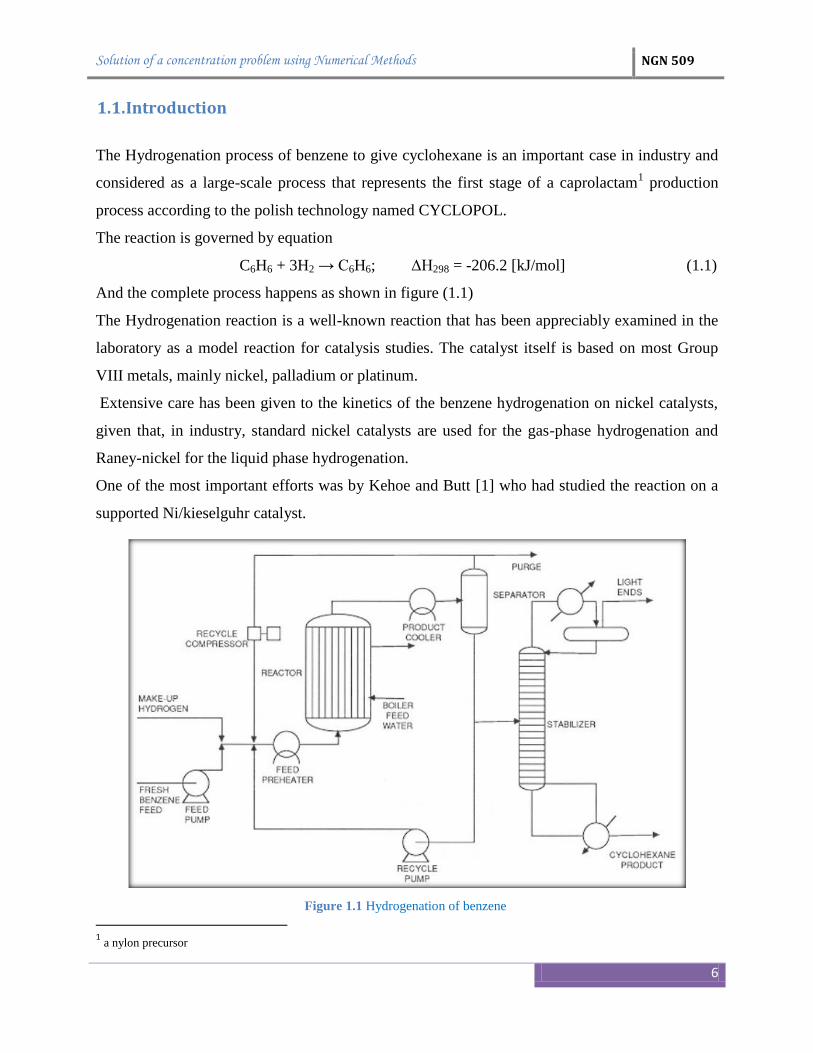
The Hydrogenation process of benzene to give cyclohexane is an important case in industry and
considered as a large-scale process that represents the first stage of a caprolactam1 production
process according to the polish technology named CYCLOPOL.
The reaction is governed by equation
C6H6 + 3H2 → C6H6; ΔH298 = -206.2 [kJ/mol] (1.1)
And the complete process happens as shown in figure (1.1)
The Hydrogenation reaction is a well-known reaction that has been appreciably examined in the
laboratory as a model reaction for catalysis studies. The catalyst itself is based on most Group
VIII metals, mainly nickel, palladium or platinum.
Extensive care has been given to the kinetics of the benzene hydrogenation on nickel catalysts,
given that, in industry, standard nickel catalysts are used for the gas-phase hydrogenation and
Raney-nickel for the liquid phase hydrogenation.
One of the most important efforts was by Kehoe and Butt [1] who had studied the reaction on a
supported Ni/kieselguhr catalyst.
1 a nylon precursor
Figure 1.1 Hydrogenation of benzene
Solution of a concentration problem using Numerical Methods NGN 509
7
They have found that in the presence of a large excess of Hydrogen, the reaction is pseudo-first-
order at temperatures below 200°C with the rate given by:
[
]
Where
Rg= gas constant, 1.987cal/(mole0K)
-Q – Ea= 2700cal/mole
PH2 = hydrogen partial pressure(torr)
k0= 4.22 mole/(gcat·s·torr)
K0 = 2.63 x10⁻⁶
cm3/(mole
0K)
T = absolute temperature (K)
CB = concentration of benzene (mole/cm3)
Price and Butt [2] studied this reaction in an isothermal tubular, plug flow reactor where a typical
run, in which (PH2 = 685 torr, ρH = density of the reactor bed = 1,2 gcat/ cm3, ϴ = constant time =
0.266 s, T = 1500C),
is used.
1.2. Problem modeling
Let
CB = feed concentration of benzene (mole/cm3)
z = axial reactor coordinate (cm)
L = reactor length
y = dimensionless concentration of benzene (CB/ CB0)
x = dimensionless axial coordinate (z/L).
The one-dimensional steady-state material balance for the reactor that expresses the fact that the
change in the axial convection of benzene is equal to the amount converted by reaction is
(
)
With CB = CB0 at x = 0
Since ϴ is constant,
[
]
mole/(g of catalyst.s) (1.2)
(1.3)
Solution of a concentration problem using Numerical Methods NGN 509
8
Gathering the constants and defining as
[
]
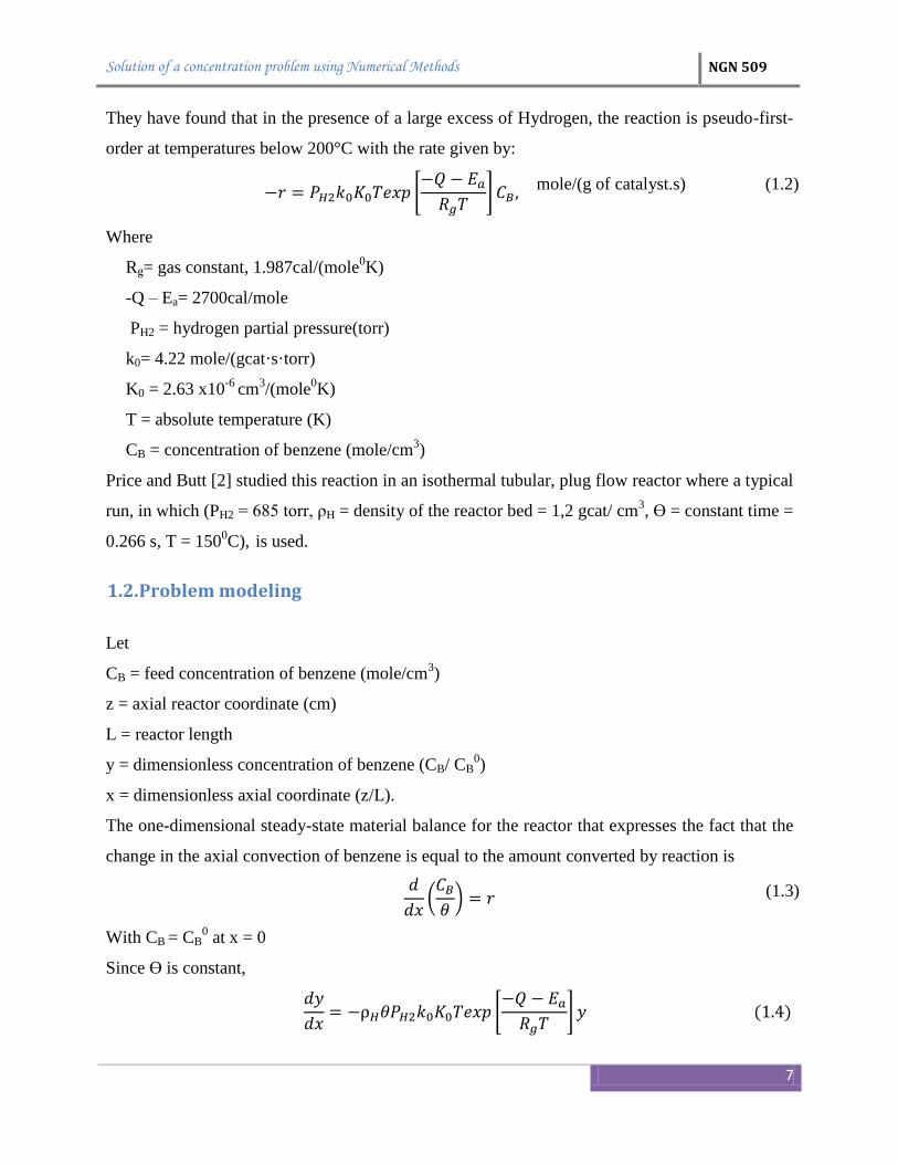
Using the data provided, it’s found = 21.6. Substituting back in (1.4)
With (y = 1 at x = 0), and the analytical solution
y = exp (-21.6 x) (1.6)
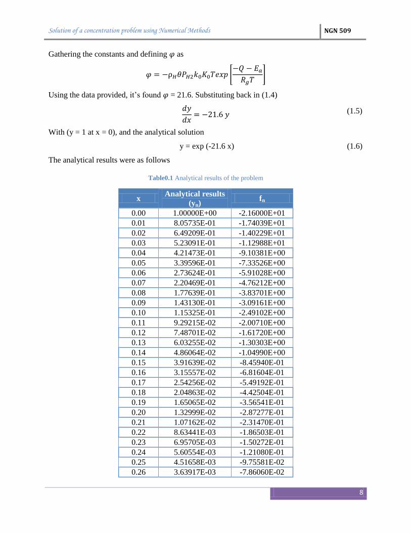
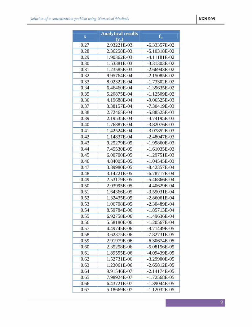
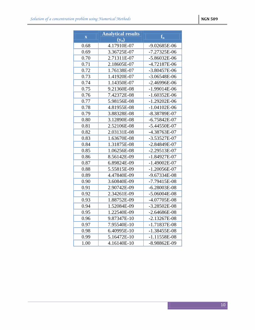
The analytical results were as follows
Table0.1 Analytical results of the problem
x Analytical results
(yn) fn
0.00 1.00000E+00 -2.16000E+01
0.01 8.05735E-01 -1.74039E+01
0.02 6.49209E-01 -1.40229E+01
0.03 5.23091E-01 -1.12988E+01
0.04 4.21473E-01 -9.10381E+00
0.05 3.39596E-01 -7.33526E+00
0.06 2.73624E-01 -5.91028E+00
0.07 2.20469E-01 -4.76212E+00
0.08 1.77639E-01 -3.83701E+00
0.09 1.43130E-01 -3.09161E+00
0.10 1.15325E-01 -2.49102E+00
0.11 9.29215E-02 -2.00710E+00
0.12 7.48701E-02 -1.61720E+00
0.13 6.03255E-02 -1.30303E+00
0.14 4.86064E-02 -1.04990E+00
0.15 3.91639E-02 -8.45940E-01
0.16 3.15557E-02 -6.81604E-01
0.17 2.54256E-02 -5.49192E-01
0.18 2.04863E-02 -4.42504E-01
0.19 1.65065E-02 -3.56541E-01
0.20 1.32999E-02 -2.87277E-01
0.21 1.07162E-02 -2.31470E-01
0.22 8.63441E-03 -1.86503E-01
0.23 6.95705E-03 -1.50272E-01
0.24 5.60554E-03 -1.21080E-01
0.25 4.51658E-03 -9.75581E-02
0.26 3.63917E-03 -7.86060E-02
(1.5)
Solution of a concentration problem using Numerical Methods NGN 509
9
x Analytical results
(yn) fn
0.27 2.93221E-03 -6.33357E-02
0.28 2.36258E-03 -5.10318E-02
0.29 1.90362E-03 -4.11181E-02
0.30 1.53381E-03 -3.31303E-02
0.31 1.23585E-03 -2.66943E-02
0.32 9.95764E-04 -2.15085E-02
0.33 8.02322E-04 -1.73302E-02
0.34 6.46460E-04 -1.39635E-02
0.35 5.20875E-04 -1.12509E-02
0.36 4.19688E-04 -9.06525E-03
0.37 3.38157E-04 -7.30419E-03
0.38 2.72465E-04 -5.88525E-03
0.39 2.19535E-04 -4.74195E-03
0.40 1.76887E-04 -3.82076E-03
0.41 1.42524E-04 -3.07852E-03
0.42 1.14837E-04 -2.48047E-03
0.43 9.25279E-05 -1.99860E-03
0.44 7.45530E-05 -1.61035E-03
0.45 6.00700E-05 -1.29751E-03
0.46 4.84005E-05 -1.04545E-03
0.47 3.89980E-05 -8.42357E-04
0.48 3.14221E-05 -6.78717E-04
0.49 2.53179E-05 -5.46866E-04
0.50 2.03995E-05 -4.40629E-04
0.51 1.64366E-05 -3.55031E-04
0.52 1.32435E-05 -2.86061E-04
0.53 1.06708E-05 -2.30489E-04
0.54 8.59784E-06 -1.85713E-04
0.55 6.92758E-06 -1.49636E-04
0.56 5.58180E-06 -1.20567E-04
0.57 4.49745E-06 -9.71449E-05
0.58 3.62375E-06 -7.82731E-05
0.59 2.91979E-06 -6.30674E-05
0.60 2.35258E-06 -5.08156E-05
0.61 1.89555E-06 -4.09439E-05
0.62 1.52731E-06 -3.29900E-05
0.63 1.23061E-06 -2.65812E-05
0.64 9.91546E-07 -2.14174E-05
0.65 7.98924E-07 -1.72568E-05
0.66 6.43721E-07 -1.39044E-05
0.67 5.18669E-07 -1.12032E-05
Solution of a concentration problem using Numerical Methods NGN 509
10
x Analytical results
(yn) fn
0.68 4.17910E-07 -9.02685E-06
0.69 3.36725E-07 -7.27325E-06
0.70 2.71311E-07 -5.86032E-06
0.71 2.18605E-07 -4.72187E-06
0.72 1.76138E-07 -3.80457E-06
0.73 1.41920E-07 -3.06548E-06
0.74 1.14350E-07 -2.46996E-06
0.75 9.21360E-08 -1.99014E-06
0.76 7.42372E-08 -1.60352E-06
0.77 5.98156E-08 -1.29202E-06
0.78 4.81955E-08 -1.04102E-06
0.79 3.88328E-08 -8.38789E-07
0.80 3.12890E-08 -6.75842E-07
0.81 2.52106E-08 -5.44550E-07
0.82 2.03131E-08 -4.38763E-07
0.83 1.63670E-08 -3.53527E-07
0.84 1.31875E-08 -2.84849E-07
0.85 1.06256E-08 -2.29513E-07
0.86 8.56142E-09 -1.84927E-07
0.87 6.89824E-09 -1.49002E-07
0.88 5.55815E-09 -1.20056E-07
0.89 4.47840E-09 -9.67334E-08
0.90 3.60840E-09 -7.79415E-08
0.91 2.90742E-09 -6.28003E-08
0.92 2.34261E-09 -5.06004E-08
0.93 1.88752E-09 -4.07705E-08
0.94 1.52084E-09 -3.28502E-08
0.95 1.22540E-09 -2.64686E-08
0.96 9.87347E-10 -2.13267E-08
0.97 7.95540E-10 -1.71837E-08
0.98 6.40995E-10 -1.38455E-08
0.99 5.16472E-10 -1.11558E-08
1.00 4.16140E-10 -8.98862E-09

Solution of a concentration problem using Numerical Methods NGN 509
11
Solution of a concentration problem using Numerical Methods NGN 509
12
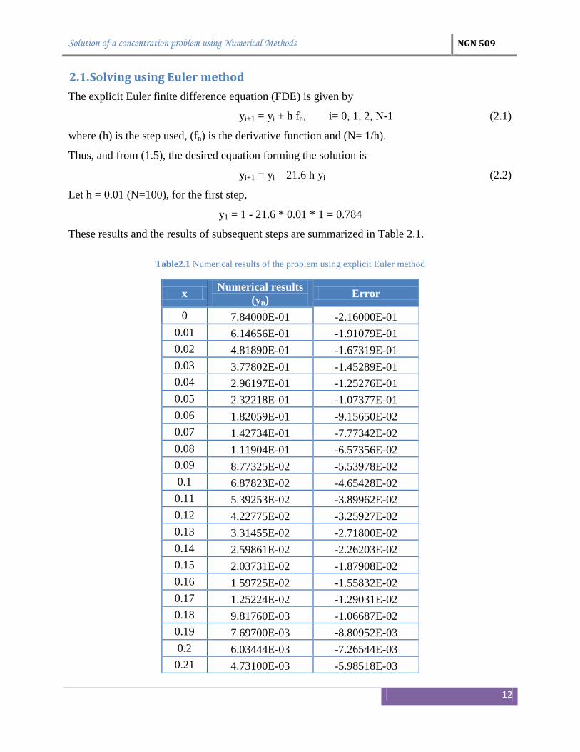
2.1. Solving using Euler method
The explicit Euler finite difference equation (FDE) is given by
yi+1 = yi + h fn, i= 0, 1, 2, N-1 (2.1)
where (h) is the step used, (fn) is the derivative function and (N= 1/h).
Thus, and from (1.5), the desired equation forming the solution is
yi+1 = yi – 21.6 h yi (2.2)
Let h = 0.01 (N=100), for the first step,
y1 = 1 - 21.6 * 0.01 * 1 = 0.784
These results and the results of subsequent steps are summarized in Table 2.1.
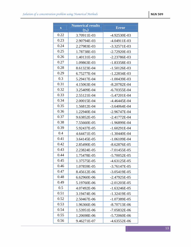
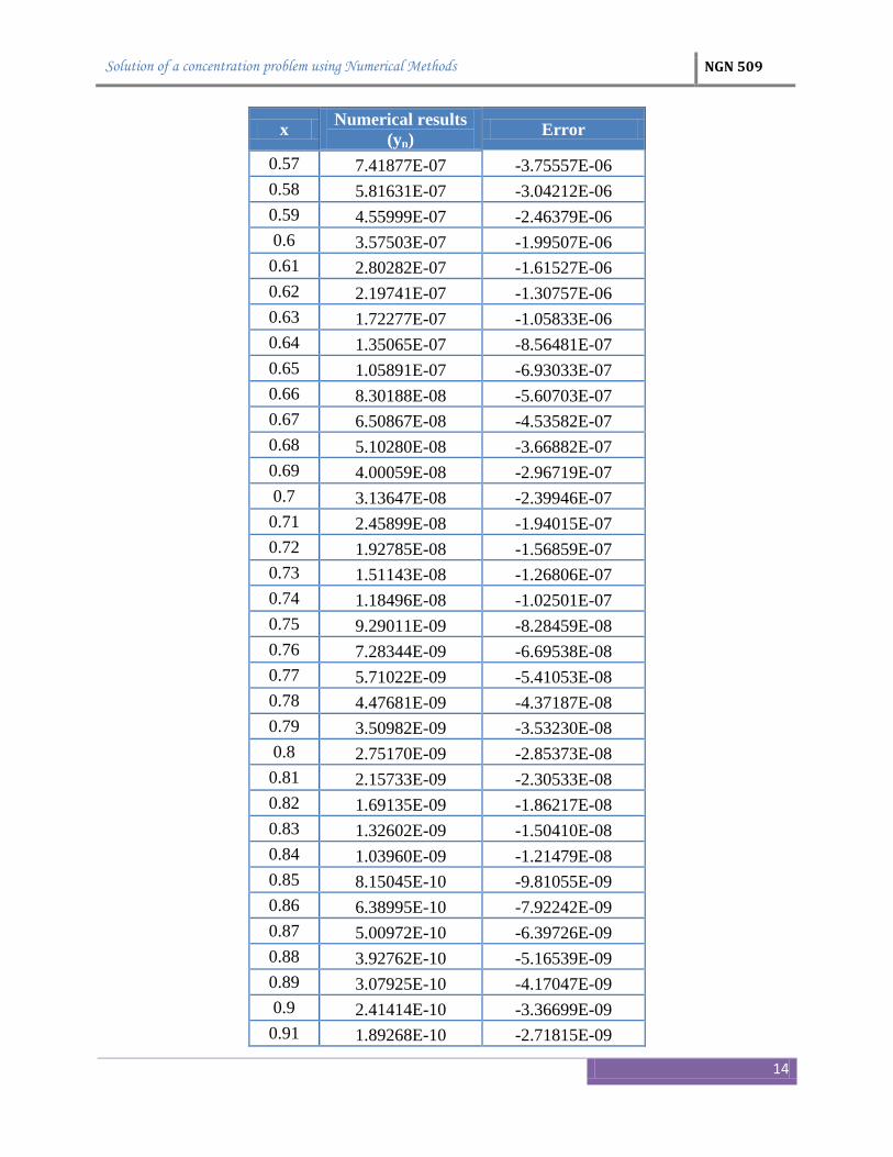
Table2.1 Numerical results of the problem using explicit Euler method
x Numerical results
(yn) Error
0 7.84000E-01 -2.16000E-01
0.01 6.14656E-01 -1.91079E-01
0.02 4.81890E-01 -1.67319E-01
0.03 3.77802E-01 -1.45289E-01
0.04 2.96197E-01 -1.25276E-01
0.05 2.32218E-01 -1.07377E-01
0.06 1.82059E-01 -9.15650E-02
0.07 1.42734E-01 -7.77342E-02
0.08 1.11904E-01 -6.57356E-02
0.09 8.77325E-02 -5.53978E-02
0.1 6.87823E-02 -4.65428E-02
0.11 5.39253E-02 -3.89962E-02
0.12 4.22775E-02 -3.25927E-02
0.13 3.31455E-02 -2.71800E-02
0.14 2.59861E-02 -2.26203E-02
0.15 2.03731E-02 -1.87908E-02
0.16 1.59725E-02 -1.55832E-02
0.17 1.25224E-02 -1.29031E-02
0.18 9.81760E-03 -1.06687E-02
0.19 7.69700E-03 -8.80952E-03
0.2 6.03444E-03 -7.26544E-03
0.21 4.73100E-03 -5.98518E-03
Solution of a concentration problem using Numerical Methods NGN 509
13
x Numerical results
(yn) Error
0.22 3.70911E-03 -4.92530E-03
0.23 2.90794E-03 -4.04911E-03
0.24 2.27983E-03 -3.32571E-03
0.25 1.78738E-03 -2.72920E-03
0.26 1.40131E-03 -2.23786E-03
0.27 1.09863E-03 -1.83358E-03
0.28 8.61323E-04 -1.50126E-03
0.29 6.75277E-04 -1.22834E-03
0.3 5.29417E-04 -1.00439E-03
0.31 4.15063E-04 -8.20782E-04
0.32 3.25409E-04 -6.70355E-04
0.33 2.55121E-04 -5.47201E-04
0.34 2.00015E-04 -4.46445E-04
0.35 1.56812E-04 -3.64064E-04
0.36 1.22940E-04 -2.96747E-04
0.37 9.63852E-05 -2.41772E-04
0.38 7.55660E-05 -1.96899E-04
0.39 5.92437E-05 -1.60291E-04
0.4 4.64471E-05 -1.30440E-04
0.41 3.64145E-05 -1.06109E-04
0.42 2.85490E-05 -8.62876E-05
0.43 2.23824E-05 -7.01455E-05
0.44 1.75478E-05 -5.70052E-05
0.45 1.37575E-05 -4.63125E-05
0.46 1.07859E-05 -3.76147E-05
0.47 8.45612E-06 -3.05419E-05
0.48 6.62960E-06 -2.47925E-05
0.49 5.19760E-06 -2.01203E-05
0.5 4.07492E-06 -1.63246E-05
0.51 3.19474E-06 -1.32419E-05
0.52 2.50467E-06 -1.07389E-05
0.53 1.96366E-06 -8.70713E-06
0.54 1.53951E-06 -7.05832E-06
0.55 1.20698E-06 -5.72060E-06
0.56 9.46271E-07 -4.63552E-06
Solution of a concentration problem using Numerical Methods NGN 509
14
x Numerical results
(yn) Error
0.57 7.41877E-07 -3.75557E-06
0.58 5.81631E-07 -3.04212E-06
0.59 4.55999E-07 -2.46379E-06
0.6 3.57503E-07 -1.99507E-06
0.61 2.80282E-07 -1.61527E-06
0.62 2.19741E-07 -1.30757E-06
0.63 1.72277E-07 -1.05833E-06
0.64 1.35065E-07 -8.56481E-07
0.65 1.05891E-07 -6.93033E-07
0.66 8.30188E-08 -5.60703E-07
0.67 6.50867E-08 -4.53582E-07
0.68 5.10280E-08 -3.66882E-07
0.69 4.00059E-08 -2.96719E-07
0.7 3.13647E-08 -2.39946E-07
0.71 2.45899E-08 -1.94015E-07
0.72 1.92785E-08 -1.56859E-07
0.73 1.51143E-08 -1.26806E-07
0.74 1.18496E-08 -1.02501E-07
0.75 9.29011E-09 -8.28459E-08
0.76 7.28344E-09 -6.69538E-08
0.77 5.71022E-09 -5.41053E-08
0.78 4.47681E-09 -4.37187E-08
0.79 3.50982E-09 -3.53230E-08
0.8 2.75170E-09 -2.85373E-08
0.81 2.15733E-09 -2.30533E-08
0.82 1.69135E-09 -1.86217E-08
0.83 1.32602E-09 -1.50410E-08
0.84 1.03960E-09 -1.21479E-08
0.85 8.15045E-10 -9.81055E-09
0.86 6.38995E-10 -7.92242E-09
0.87 5.00972E-10 -6.39726E-09
0.88 3.92762E-10 -5.16539E-09
0.89 3.07925E-10 -4.17047E-09
0.9 2.41414E-10 -3.36699E-09
0.91 1.89268E-10 -2.71815E-09
Solution of a concentration problem using Numerical Methods NGN 509
15
x Numerical results
(yn) Error
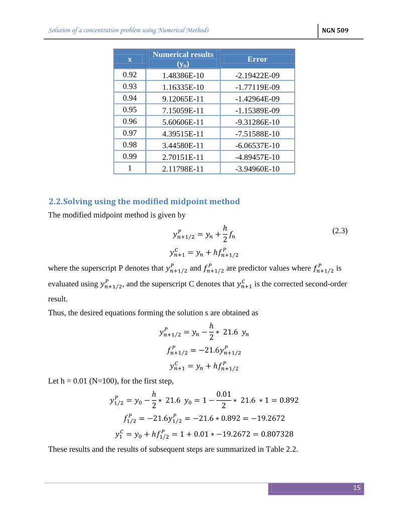
0.92 1.48386E-10 -2.19422E-09
0.93 1.16335E-10 -1.77119E-09
0.94 9.12065E-11 -1.42964E-09
0.95 7.15059E-11 -1.15389E-09
0.96 5.60606E-11 -9.31286E-10
0.97 4.39515E-11 -7.51588E-10
0.98 3.44580E-11 -6.06537E-10
0.99 2.70151E-11 -4.89457E-10
1 2.11798E-11 -3.94960E-10
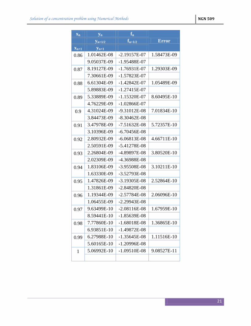
2.2. Solving using the modified midpoint method
The modified midpoint method is given by
⁄
⁄
where the superscript P denotes that ⁄ and ⁄
are predictor values where ⁄ is
evaluated using ⁄ , and the superscript C denotes that
is the corrected second-order
result.
Thus, the desired equations forming the solution s are obtained as
⁄
⁄ ⁄
⁄
Let h = 0.01 (N=100), for the first step,
⁄
⁄ ⁄
⁄
These results and the results of subsequent steps are summarized in Table 2.2.
(2.3)
Solution of a concentration problem using Numerical Methods NGN 509
16
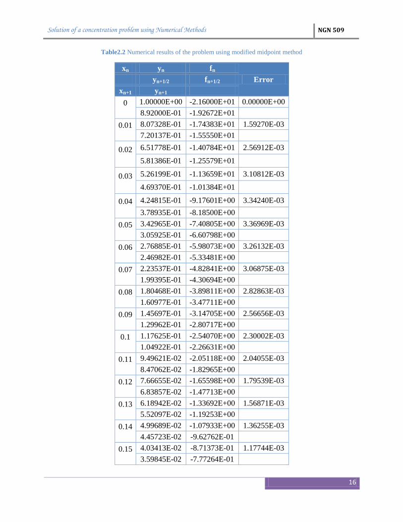
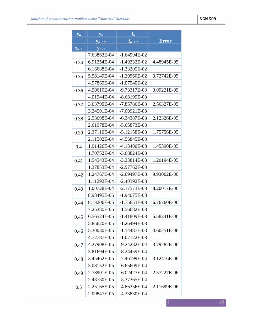
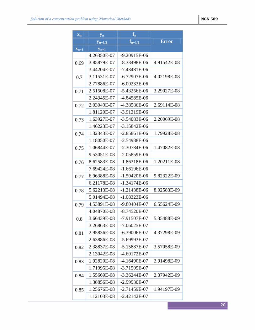
Table2.2 Numerical results of the problem using modified midpoint method
xn yn fn
Error yn+1/2 fn+1/2
xn+1 yn+1
0
1.00000E+00 -2.16000E+01 0.00000E+00
8.92000E-01 -1.92672E+01
0.01
8.07328E-01 -1.74383E+01 1.59270E-03
7.20137E-01 -1.55550E+01
0.02
6.51778E-01 -1.40784E+01 2.56912E-03
5.81386E-01 -1.25579E+01
0.03
5.26199E-01 -1.13659E+01 3.10812E-03
4.69370E-01 -1.01384E+01
0.04
4.24815E-01 -9.17601E+00 3.34240E-03
3.78935E-01 -8.18500E+00
0.05
3.42965E-01 -7.40805E+00 3.36969E-03
3.05925E-01 -6.60798E+00
0.06
2.76885E-01 -5.98073E+00 3.26132E-03
2.46982E-01 -5.33481E+00
0.07
2.23537E-01 -4.82841E+00 3.06875E-03
1.99395E-01 -4.30694E+00
0.08
1.80468E-01 -3.89811E+00 2.82863E-03
1.60977E-01 -3.47711E+00
0.09
1.45697E-01 -3.14705E+00 2.56656E-03
1.29962E-01 -2.80717E+00
0.1
1.17625E-01 -2.54070E+00 2.30002E-03
1.04922E-01 -2.26631E+00
0.11
9.49621E-02 -2.05118E+00 2.04055E-03
8.47062E-02 -1.82965E+00
0.12
7.66655E-02 -1.65598E+00 1.79539E-03
6.83857E-02 -1.47713E+00
0.13
6.18942E-02 -1.33692E+00 1.56871E-03
5.52097E-02 -1.19253E+00
0.14
4.99689E-02 -1.07933E+00 1.36255E-03
4.45723E-02 -9.62762E-01
0.15
4.03413E-02 -8.71373E-01 1.17744E-03
3.59845E-02 -7.77264E-01

Solution of a concentration problem using Numerical Methods NGN 509
17
xn yn fn
Error yn+1/2 fn+1/2
xn+1 yn+1
0.16
3.25687E-02 -7.03484E-01 1.01295E-03
2.90513E-02 -6.27507E-01
0.17
2.62936E-02 -5.67942E-01 8.68044E-04
2.34539E-02 -5.06604E-01
0.18
2.12276E-02 -4.58516E-01 7.41292E-04
1.89350E-02 -4.08996E-01
0.19
1.71376E-02 -3.70172E-01 6.31094E-04
1.52867E-02 -3.30194E-01
0.2
1.38357E-02 -2.98851E-01 5.35790E-04
1.23414E-02 -2.66575E-01
0.21
1.11699E-02 -2.41270E-01 4.53741E-04
9.96357E-03 -2.15213E-01
0.22
9.01779E-03 -1.94784E-01 3.83385E-04
8.04387E-03 -1.73748E-01
0.23
7.28032E-03 -1.57255E-01 3.23270E-04
6.49404E-03 -1.40271E-01
0.24
5.87760E-03 -1.26956E-01 2.72065E-04
5.24282E-03 -1.13245E-01
0.25
4.74515E-03 -1.02495E-01 2.28574E-04
4.23268E-03 -9.14258E-02
0.26
3.83090E-03 -8.27474E-02 1.91728E-04
3.41716E-03 -7.38106E-02
0.27
3.09279E-03 -6.68043E-02 1.60583E-04
2.75877E-03 -5.95894E-02
0.28
2.49690E-03 -5.39329E-02 1.34313E-04
2.22723E-03 -4.81082E-02
0.29
2.01581E-03 -4.35416E-02 1.12198E-04
1.79811E-03 -3.88391E-02
0.3
1.62742E-03 -3.51523E-02 9.36123E-05
1.45166E-03 -3.13559E-02
0.31
1.31386E-03 -2.83795E-02 7.80188E-05
1.17197E-03 -2.53145E-02
0.32
1.06072E-03 -2.29115E-02 6.49551E-05
9.46162E-04 -2.04371E-02
0.33 8.56348E-04 -1.84971E-02 5.40260E-05
Solution of a concentration problem using Numerical Methods NGN 509
18
xn yn fn
Error yn+1/2 fn+1/2
xn+1 yn+1
7.63863E-04 -1.64994E-02
0.34
6.91354E-04 -1.49332E-02 4.48945E-05
6.16688E-04 -1.33205E-02
0.35
5.58149E-04 -1.20560E-02 3.72742E-05
4.97869E-04 -1.07540E-02
0.36
4.50610E-04 -9.73317E-03 3.09221E-05
4.01944E-04 -8.68199E-03
0.37
3.63790E-04 -7.85786E-03 2.56327E-05
3.24501E-04 -7.00921E-03
0.38
2.93698E-04 -6.34387E-03 2.12326E-05
2.61978E-04 -5.65873E-03
0.39
2.37110E-04 -5.12158E-03 1.75756E-05
2.11502E-04 -4.56845E-03
0.4
1.91426E-04 -4.13480E-03 1.45390E-05
1.70752E-04 -3.68824E-03
0.41
1.54543E-04 -3.33814E-03 1.20194E-05
1.37853E-04 -2.97762E-03
0.42
1.24767E-04 -2.69497E-03 9.93062E-06
1.11292E-04 -2.40392E-03
0.43
1.00728E-04 -2.17573E-03 8.20017E-06
8.98495E-05 -1.94075E-03
0.44
8.13206E-05 -1.75653E-03 6.76760E-06
7.25380E-05 -1.56682E-03
0.45
6.56524E-05 -1.41809E-03 5.58241E-06
5.85620E-05 -1.26494E-03
0.46
5.30030E-05 -1.14487E-03 4.60251E-06
4.72787E-05 -1.02122E-03
0.47
4.27908E-05 -9.24282E-04 3.79282E-06
3.81694E-05 -8.24459E-04
0.48
3.45462E-05 -7.46199E-04 3.12416E-06
3.08152E-05 -6.65609E-04
0.49
2.78901E-05 -6.02427E-04 2.57227E-06
2.48780E-05 -5.37365E-04
0.5
2.25165E-05 -4.86356E-04 2.11699E-06
2.00847E-05 -4.33830E-04

Solution of a concentration problem using Numerical Methods NGN 509
19
xn yn fn
Error yn+1/2 fn+1/2
xn+1 yn+1
0.51
1.81782E-05 -3.92649E-04 1.74160E-06
1.62150E-05 -3.50243E-04
0.52
1.46758E-05 -3.16997E-04 1.43222E-06
1.30908E-05 -2.82761E-04
0.53
1.18482E-05 -2.55920E-04 1.17736E-06
1.05686E-05 -2.28281E-04
0.54
9.56535E-06 -2.06612E-04 9.67513E-07
8.53229E-06 -1.84297E-04
0.55
7.72237E-06 -1.66803E-04 7.94794E-07
6.88836E-06 -1.48789E-04
0.56
6.23449E-06 -1.34665E-04 6.52693E-07
5.56116E-06 -1.20121E-04
0.57
5.03328E-06 -1.08719E-04 5.35827E-07
4.48968E-06 -9.69772E-05
0.58
4.06351E-06 -8.77717E-05 4.39752E-07
3.62465E-06 -7.82924E-05
0.59
3.28058E-06 -7.08606E-05 3.60795E-07
2.92628E-06 -6.32076E-05
0.6
2.64851E-06 -5.72077E-05 2.95930E-07
2.36247E-06 -5.10293E-05
0.61
2.13821E-06 -4.61854E-05 2.42660E-07
1.90729E-06 -4.11974E-05
0.62
1.72624E-06 -3.72868E-05 1.98925E-07
1.53981E-06 -3.32598E-05
0.63
1.39364E-06 -3.01026E-05 1.63030E-07
1.24313E-06 -2.68516E-05
0.64
1.12513E-06 -2.43027E-05 1.33579E-07
1.00361E-06 -2.16780E-05
0.65
9.08345E-07 -1.96203E-05 1.09421E-07
8.10244E-07 -1.75013E-05
0.66
7.33333E-07 -1.58400E-05 8.96113E-08
6.54133E-07 -1.41293E-05
0.67
5.92040E-07 -1.27881E-05 7.33710E-08
5.28100E-07 -1.14070E-05
0.68 4.77970E-07 -1.03242E-05 6.00605E-08
Solution of a concentration problem using Numerical Methods NGN 509
20
xn yn fn
Error yn+1/2 fn+1/2
xn+1 yn+1
4.26350E-07 -9.20915E-06
0.69
3.85879E-07 -8.33498E-06 4.91542E-08
3.44204E-07 -7.43481E-06
0.7
3.11531E-07 -6.72907E-06 4.02198E-08
2.77886E-07 -6.00233E-06
0.71
2.51508E-07 -5.43256E-06 3.29027E-08
2.24345E-07 -4.84585E-06
0.72
2.03049E-07 -4.38586E-06 2.69114E-08
1.81120E-07 -3.91219E-06
0.73
1.63927E-07 -3.54083E-06 2.20069E-08
1.46223E-07 -3.15842E-06
0.74
1.32343E-07 -2.85861E-06 1.79928E-08
1.18050E-07 -2.54988E-06
0.75
1.06844E-07 -2.30784E-06 1.47082E-08
9.53051E-08 -2.05859E-06
0.76
8.62583E-08 -1.86318E-06 1.20211E-08
7.69424E-08 -1.66196E-06
0.77
6.96388E-08 -1.50420E-06 9.82322E-09
6.21178E-08 -1.34174E-06
0.78
5.62213E-08 -1.21438E-06 8.02583E-09
5.01494E-08 -1.08323E-06
0.79
4.53891E-08 -9.80404E-07 6.55624E-09
4.04870E-08 -8.74520E-07
0.8
3.66439E-08 -7.91507E-07 5.35488E-09
3.26863E-08 -7.06025E-07
0.81
2.95836E-08 -6.39006E-07 4.37298E-09
2.63886E-08 -5.69993E-07
0.82
2.38837E-08 -5.15887E-07 3.57058E-09
2.13042E-08 -4.60172E-07
0.83
1.92820E-08 -4.16490E-07 2.91498E-09
1.71995E-08 -3.71509E-07
0.84
1.55669E-08 -3.36244E-07 2.37942E-09
1.38856E-08 -2.99930E-07
0.85
1.25676E-08 -2.71459E-07 1.94197E-09
1.12103E-08 -2.42142E-07
Solution of a concentration problem using Numerical Methods NGN 509
21
xn yn fn
Error yn+1/2 fn+1/2
xn+1 yn+1
0.86
1.01462E-08 -2.19157E-07 1.58473E-09
9.05037E-09 -1.95488E-07
0.87
8.19127E-09 -1.76931E-07 1.29303E-09
7.30661E-09 -1.57823E-07
0.88
6.61304E-09 -1.42842E-07 1.05489E-09
5.89883E-09 -1.27415E-07
0.89
5.33889E-09 -1.15320E-07 8.60495E-10
4.76229E-09 -1.02866E-07
0.9
4.31024E-09 -9.31012E-08 7.01834E-10
3.84473E-09 -8.30462E-08
0.91
3.47978E-09 -7.51632E-08 5.72357E-10
3.10396E-09 -6.70456E-08
0.92
2.80932E-09 -6.06813E-08 4.66711E-10
2.50591E-09 -5.41278E-08
0.93
2.26804E-09 -4.89897E-08 3.80520E-10
2.02309E-09 -4.36988E-08
0.94
1.83106E-09 -3.95508E-08 3.10211E-10
1.63330E-09 -3.52793E-08
0.95
1.47826E-09 -3.19305E-08 2.52864E-10
1.31861E-09 -2.84820E-08
0.96
1.19344E-09 -2.57784E-08 2.06096E-10
1.06455E-09 -2.29943E-08
0.97
9.63499E-10 -2.08116E-08 1.67959E-10
8.59441E-10 -1.85639E-08
0.98
7.77860E-10 -1.68018E-08 1.36865E-10
6.93851E-10 -1.49872E-08
0.99
6.27988E-10 -1.35645E-08 1.11516E-10
5.60165E-10 -1.20996E-08
1
5.06992E-10 -1.09510E-08 9.08527E-11
Solution of a concentration problem using Numerical Methods NGN 509
22
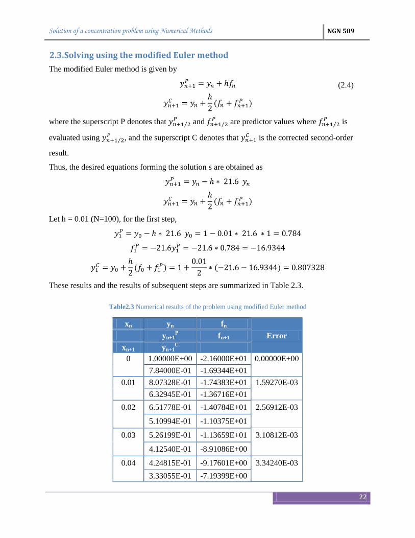
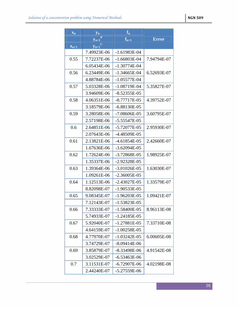
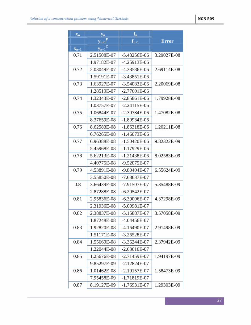
2.3. Solving using the modified Euler method
The modified Euler method is given by
where the superscript P denotes that ⁄ and ⁄
are predictor values where ⁄ is
evaluated using ⁄ , and the superscript C denotes that
is the corrected second-order
result.
Thus, the desired equations forming the solution s are obtained as
Let h = 0.01 (N=100), for the first step,
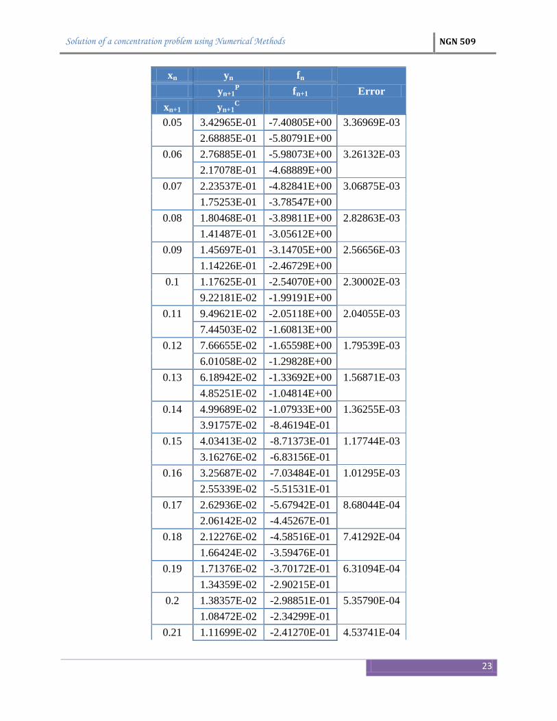
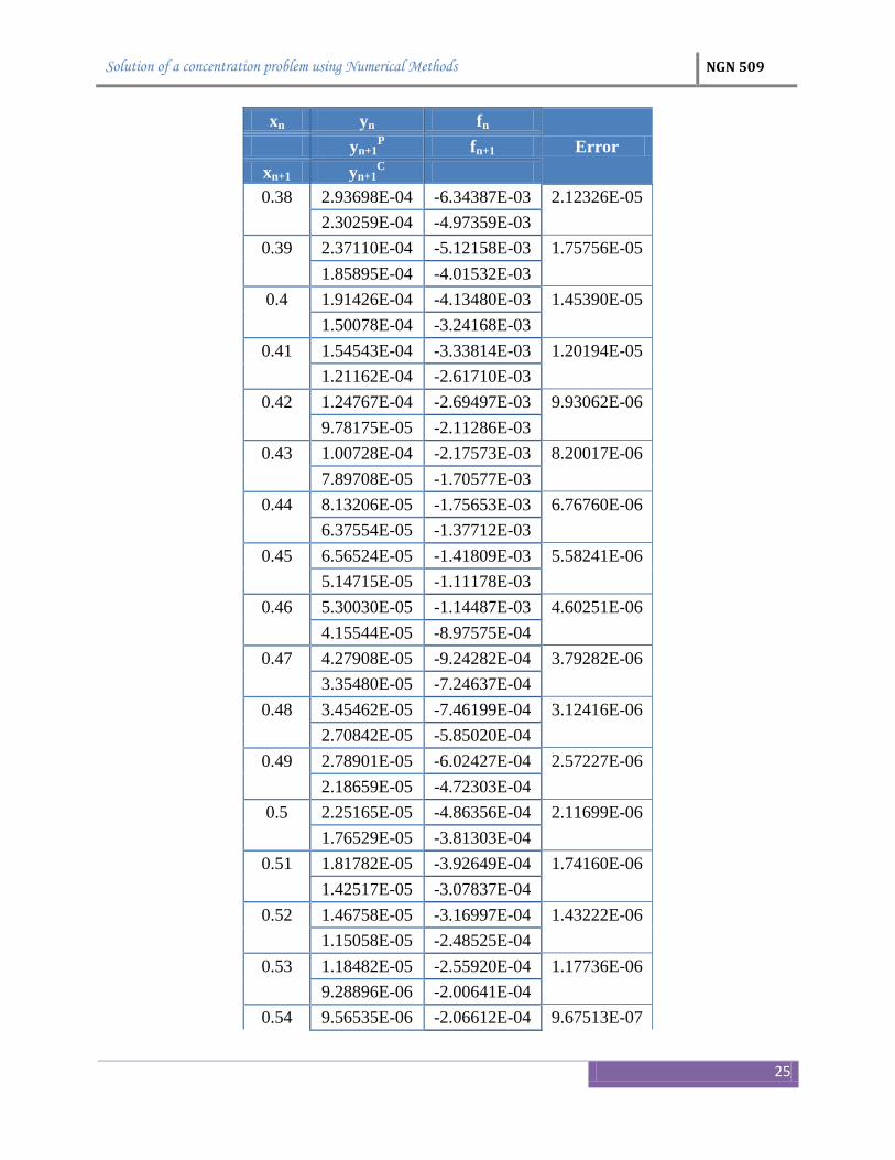
These results and the results of subsequent steps are summarized in Table 2.3.
Table2.3 Numerical results of the problem using modified Euler method
xn yn fn
Error yn+1P fn+1
xn+1 yn+1C
0 1.00000E+00 -2.16000E+01 0.00000E+00
7.84000E-01 -1.69344E+01
0.01 8.07328E-01 -1.74383E+01 1.59270E-03
6.32945E-01 -1.36716E+01
0.02 6.51778E-01 -1.40784E+01 2.56912E-03
5.10994E-01 -1.10375E+01
0.03 5.26199E-01 -1.13659E+01 3.10812E-03
4.12540E-01 -8.91086E+00
0.04 4.24815E-01 -9.17601E+00 3.34240E-03
3.33055E-01 -7.19399E+00
(2.4)
Solution of a concentration problem using Numerical Methods NGN 509
23
xn yn fn
Error yn+1P fn+1
xn+1 yn+1C
0.05 3.42965E-01 -7.40805E+00 3.36969E-03
2.68885E-01 -5.80791E+00
0.06 2.76885E-01 -5.98073E+00 3.26132E-03
2.17078E-01 -4.68889E+00
0.07 2.23537E-01 -4.82841E+00 3.06875E-03
1.75253E-01 -3.78547E+00
0.08 1.80468E-01 -3.89811E+00 2.82863E-03
1.41487E-01 -3.05612E+00
0.09 1.45697E-01 -3.14705E+00 2.56656E-03
1.14226E-01 -2.46729E+00
0.1 1.17625E-01 -2.54070E+00 2.30002E-03
9.22181E-02 -1.99191E+00
0.11 9.49621E-02 -2.05118E+00 2.04055E-03
7.44503E-02 -1.60813E+00
0.12 7.66655E-02 -1.65598E+00 1.79539E-03
6.01058E-02 -1.29828E+00
0.13 6.18942E-02 -1.33692E+00 1.56871E-03
4.85251E-02 -1.04814E+00
0.14 4.99689E-02 -1.07933E+00 1.36255E-03
3.91757E-02 -8.46194E-01
0.15 4.03413E-02 -8.71373E-01 1.17744E-03
3.16276E-02 -6.83156E-01
0.16 3.25687E-02 -7.03484E-01 1.01295E-03
2.55339E-02 -5.51531E-01
0.17 2.62936E-02 -5.67942E-01 8.68044E-04
2.06142E-02 -4.45267E-01
0.18 2.12276E-02 -4.58516E-01 7.41292E-04
1.66424E-02 -3.59476E-01
0.19 1.71376E-02 -3.70172E-01 6.31094E-04
1.34359E-02 -2.90215E-01
0.2 1.38357E-02 -2.98851E-01 5.35790E-04
1.08472E-02 -2.34299E-01
0.21 1.11699E-02 -2.41270E-01 4.53741E-04

Solution of a concentration problem using Numerical Methods NGN 509
24
xn yn fn
Error yn+1P fn+1
xn+1 yn+1C
8.75722E-03 -1.89156E-01
0.22 9.01779E-03 -1.94784E-01 3.83385E-04
7.06995E-03 -1.52711E-01
0.23 7.28032E-03 -1.57255E-01 3.23270E-04
5.70777E-03 -1.23288E-01
0.24 5.87760E-03 -1.26956E-01 2.72065E-04
4.60804E-03 -9.95337E-02
0.25 4.74515E-03 -1.02495E-01 2.28574E-04
3.72020E-03 -8.03563E-02
0.26 3.83090E-03 -8.27474E-02 1.91728E-04
3.00342E-03 -6.48739E-02
0.27 3.09279E-03 -6.68043E-02 1.60583E-04
2.42475E-03 -5.23745E-02
0.28 2.49690E-03 -5.39329E-02 1.34313E-04
1.95757E-03 -4.22834E-02
0.29 2.01581E-03 -4.35416E-02 1.12198E-04
1.58040E-03 -3.41366E-02
0.3 1.62742E-03 -3.51523E-02 9.36123E-05
1.27590E-03 -2.75594E-02
0.31 1.31386E-03 -2.83795E-02 7.80188E-05
1.03007E-03 -2.22495E-02
0.32 1.06072E-03 -2.29115E-02 6.49551E-05
8.31604E-04 -1.79626E-02
0.33 8.56348E-04 -1.84971E-02 5.40260E-05
6.71377E-04 -1.45017E-02
0.34 6.91354E-04 -1.49332E-02 4.48945E-05
5.42022E-04 -1.17077E-02
0.35 5.58149E-04 -1.20560E-02 3.72742E-05
4.37589E-04 -9.45193E-03
0.36 4.50610E-04 -9.73317E-03 3.09221E-05
3.53278E-04 -7.63081E-03
0.37 3.63790E-04 -7.85786E-03 2.56327E-05
2.85211E-04 -6.16056E-03
Solution of a concentration problem using Numerical Methods NGN 509
25
xn yn fn
Error yn+1P fn+1
xn+1 yn+1C
0.38 2.93698E-04 -6.34387E-03 2.12326E-05
2.30259E-04 -4.97359E-03
0.39 2.37110E-04 -5.12158E-03 1.75756E-05
1.85895E-04 -4.01532E-03
0.4 1.91426E-04 -4.13480E-03 1.45390E-05
1.50078E-04 -3.24168E-03
0.41 1.54543E-04 -3.33814E-03 1.20194E-05
1.21162E-04 -2.61710E-03
0.42 1.24767E-04 -2.69497E-03 9.93062E-06
9.78175E-05 -2.11286E-03
0.43 1.00728E-04 -2.17573E-03 8.20017E-06
7.89708E-05 -1.70577E-03
0.44 8.13206E-05 -1.75653E-03 6.76760E-06
6.37554E-05 -1.37712E-03
0.45 6.56524E-05 -1.41809E-03 5.58241E-06
5.14715E-05 -1.11178E-03
0.46 5.30030E-05 -1.14487E-03 4.60251E-06
4.15544E-05 -8.97575E-04
0.47 4.27908E-05 -9.24282E-04 3.79282E-06
3.35480E-05 -7.24637E-04
0.48 3.45462E-05 -7.46199E-04 3.12416E-06
2.70842E-05 -5.85020E-04
0.49 2.78901E-05 -6.02427E-04 2.57227E-06
2.18659E-05 -4.72303E-04
0.5 2.25165E-05 -4.86356E-04 2.11699E-06
1.76529E-05 -3.81303E-04
0.51 1.81782E-05 -3.92649E-04 1.74160E-06
1.42517E-05 -3.07837E-04
0.52 1.46758E-05 -3.16997E-04 1.43222E-06
1.15058E-05 -2.48525E-04
0.53 1.18482E-05 -2.55920E-04 1.17736E-06
9.28896E-06 -2.00641E-04
0.54 9.56535E-06 -2.06612E-04 9.67513E-07
Solution of a concentration problem using Numerical Methods NGN 509
26
xn yn fn
Error yn+1P fn+1
xn+1 yn+1C
7.49923E-06 -1.61983E-04
0.55 7.72237E-06 -1.66803E-04 7.94794E-07
6.05434E-06 -1.30774E-04
0.56 6.23449E-06 -1.34665E-04 6.52693E-07
4.88784E-06 -1.05577E-04
0.57 5.03328E-06 -1.08719E-04 5.35827E-07
3.94609E-06 -8.52355E-05
0.58 4.06351E-06 -8.77717E-05 4.39752E-07
3.18579E-06 -6.88130E-05
0.59 3.28058E-06 -7.08606E-05 3.60795E-07
2.57198E-06 -5.55547E-05
0.6 2.64851E-06 -5.72077E-05 2.95930E-07
2.07643E-06 -4.48509E-05
0.61 2.13821E-06 -4.61854E-05 2.42660E-07
1.67636E-06 -3.62094E-05
0.62 1.72624E-06 -3.72868E-05 1.98925E-07
1.35337E-06 -2.92328E-05
0.63 1.39364E-06 -3.01026E-05 1.63030E-07
1.09261E-06 -2.36005E-05
0.64 1.12513E-06 -2.43027E-05 1.33579E-07
8.82098E-07 -1.90533E-05
0.65 9.08345E-07 -1.96203E-05 1.09421E-07
7.12143E-07 -1.53823E-05
0.66 7.33333E-07 -1.58400E-05 8.96113E-08
5.74933E-07 -1.24185E-05
0.67 5.92040E-07 -1.27881E-05 7.33710E-08
4.64159E-07 -1.00258E-05
0.68 4.77970E-07 -1.03242E-05 6.00605E-08
3.74729E-07 -8.09414E-06
0.69 3.85879E-07 -8.33498E-06 4.91542E-08
3.02529E-07 -6.53463E-06
0.7 3.11531E-07 -6.72907E-06 4.02198E-08
2.44240E-07 -5.27559E-06
Solution of a concentration problem using Numerical Methods NGN 509
27
xn yn fn
Error yn+1P fn+1
xn+1 yn+1C
0.71 2.51508E-07 -5.43256E-06 3.29027E-08
1.97182E-07 -4.25913E-06
0.72 2.03049E-07 -4.38586E-06 2.69114E-08
1.59191E-07 -3.43851E-06
0.73 1.63927E-07 -3.54083E-06 2.20069E-08
1.28519E-07 -2.77601E-06
0.74 1.32343E-07 -2.85861E-06 1.79928E-08
1.03757E-07 -2.24115E-06
0.75 1.06844E-07 -2.30784E-06 1.47082E-08
8.37659E-08 -1.80934E-06
0.76 8.62583E-08 -1.86318E-06 1.20211E-08
6.76265E-08 -1.46073E-06
0.77 6.96388E-08 -1.50420E-06 9.82322E-09
5.45968E-08 -1.17929E-06
0.78 5.62213E-08 -1.21438E-06 8.02583E-09
4.40775E-08 -9.52075E-07
0.79 4.53891E-08 -9.80404E-07 6.55624E-09
3.55850E-08 -7.68637E-07
0.8 3.66439E-08 -7.91507E-07 5.35488E-09
2.87288E-08 -6.20542E-07
0.81 2.95836E-08 -6.39006E-07 4.37298E-09
2.31936E-08 -5.00981E-07
0.82 2.38837E-08 -5.15887E-07 3.57058E-09
1.87248E-08 -4.04456E-07
0.83 1.92820E-08 -4.16490E-07 2.91498E-09
1.51171E-08 -3.26528E-07
0.84 1.55669E-08 -3.36244E-07 2.37942E-09
1.22044E-08 -2.63616E-07
0.85 1.25676E-08 -2.71459E-07 1.94197E-09
9.85297E-09 -2.12824E-07
0.86 1.01462E-08 -2.19157E-07 1.58473E-09
7.95458E-09 -1.71819E-07
0.87 8.19127E-09 -1.76931E-07 1.29303E-09

Solution of a concentration problem using Numerical Methods NGN 509
28
xn yn fn
Error yn+1P fn+1
xn+1 yn+1C
6.42196E-09 -1.38714E-07
0.88 6.61304E-09 -1.42842E-07 1.05489E-09
5.18463E-09 -1.11988E-07
0.89 5.33889E-09 -1.15320E-07 8.60495E-10
4.18569E-09 -9.04110E-08
0.9 4.31024E-09 -9.31012E-08 7.01834E-10
3.37923E-09 -7.29913E-08
0.91 3.47978E-09 -7.51632E-08 5.72357E-10
2.72814E-09 -5.89279E-08
0.92 2.80932E-09 -6.06813E-08 4.66711E-10
2.20251E-09 -4.75742E-08
0.93 2.26804E-09 -4.89897E-08 3.80520E-10
1.77815E-09 -3.84080E-08
0.94 1.83106E-09 -3.95508E-08 3.10211E-10
1.43555E-09 -3.10078E-08
0.95 1.47826E-09 -3.19305E-08 2.52864E-10
1.15896E-09 -2.50335E-08
0.96 1.19344E-09 -2.57784E-08 2.06096E-10
9.35659E-10 -2.02102E-08
0.97 9.63499E-10 -2.08116E-08 1.67959E-10
7.55384E-10 -1.63163E-08
0.98 7.77860E-10 -1.68018E-08 1.36865E-10
6.09842E-10 -1.31726E-08
0.99 6.27988E-10 -1.35645E-08 1.11516E-10
4.92343E-10 -1.06346E-08
1 5.06992E-10 -1.09510E-08 9.08527E-11
3.97482E-10 -8.58561E-09
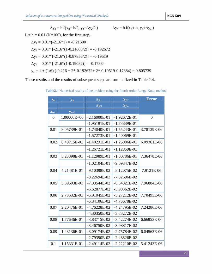
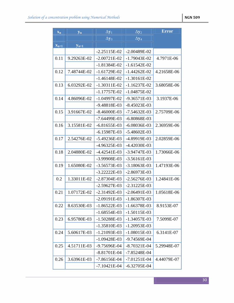
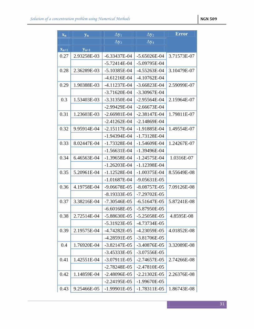
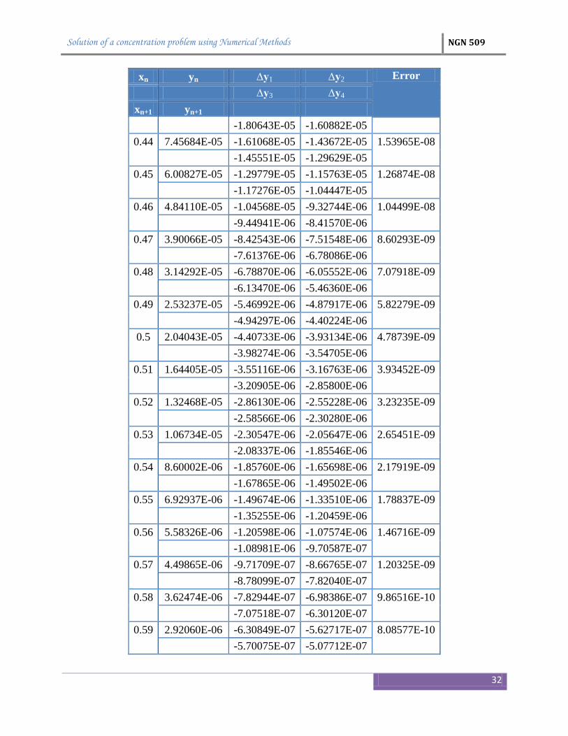
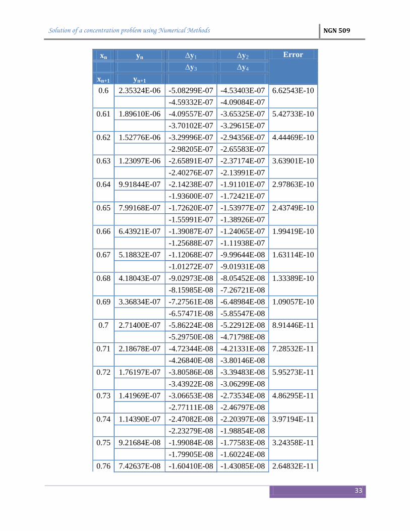
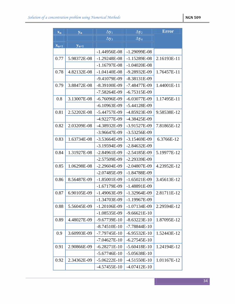
2.4. Solving using the fourth-order Runge-Kutta method
The fourth-order Runge-Kutta method is given by
yn+1 = yn + (1/6) (∆y1 + 2 ∆y2 + 2 ∆y3 + ∆y4)
∆y1 = h f(xn, yn) ∆y2 = h f(xn+ h/2, yn+∆y1/2 )
(2.5)
Solution of a concentration problem using Numerical Methods NGN 509
29
∆y3 = h f(xn+ h/2, yn+∆y2/2 ) ∆y4 = h f(xn+ h, yn+∆y3 )
Let h = 0.01 (N=100), for the first step,
∆y1 = 0.01*(-21.6*1) = -0.21600
∆y2 = 0.01* [-21.6*(1-0.21600/2)] = -0.192672
∆y3 = 0.01* [-21.6*(1-0.87856/2)] = -0.19519
∆y4 = 0.01* [-21.6*(1-0.19082)] = -0.17384
y1 = 1 + (1/6) (-0.216 + 2*-0.192672+ 2*-0.19519-0.17384) = 0.805739
These results and the results of subsequent steps are summarized in Table 2.4.
Table2.4 Numerical results of the problem using the fourth-order Runge-Kutta method
xn yn ∆y1 ∆y2 Error
∆y3 ∆y4
xn+1 yn+1
0 1.00000E+00 -2.16000E-01 -1.92672E-01 0
-1.95191E-01 -1.73839E-01
0.01 8.05739E-01 -1.74040E-01 -1.55243E-01 3.78139E-06
-1.57273E-01 -1.40069E-01
0.02 6.49215E-01 -1.40231E-01 -1.25086E-01 6.09361E-06
-1.26721E-01 -1.12859E-01
0.03 5.23098E-01 -1.12989E-01 -1.00786E-01 7.36478E-06
-1.02104E-01 -9.09347E-02
0.04 4.21481E-01 -9.10398E-02 -8.12075E-02 7.9121E-06
-8.22694E-02 -7.32696E-02
0.05 3.39603E-01 -7.33544E-02 -6.54321E-02 7.96884E-06
-6.62877E-02 -5.90362E-02
0.06 2.73632E-01 -5.91045E-02 -5.27212E-02 7.70495E-06
-5.34106E-02 -4.75678E-02
0.07 2.20476E-01 -4.76228E-02 -4.24795E-02 7.24286E-06
-4.30350E-02 -3.83272E-02
0.08 1.77646E-01 -3.83715E-02 -3.42274E-02 6.66953E-06
-3.46750E-02 -3.08817E-02
0.09 1.43136E-01 -3.09174E-02 -2.75784E-02 6.04563E-06
-2.79390E-02 -2.48826E-02
0.1 1.15331E-01 -2.49114E-02 -2.22210E-02 5.41243E-06
Solution of a concentration problem using Numerical Methods NGN 509
30
xn yn ∆y1 ∆y2 Error
∆y3 ∆y4
xn+1 yn+1
-2.25115E-02 -2.00489E-02
0.11 9.29263E-02 -2.00721E-02 -1.79043E-02 4.7971E-06
-1.81384E-02 -1.61542E-02
0.12 7.48744E-02 -1.61729E-02 -1.44262E-02 4.21658E-06
-1.46148E-02 -1.30161E-02
0.13 6.03292E-02 -1.30311E-02 -1.16237E-02 3.68058E-06
-1.17757E-02 -1.04875E-02
0.14 4.86096E-02 -1.04997E-02 -9.36571E-03 3.1937E-06
-9.48818E-03 -8.45023E-03
0.15 3.91667E-02 -8.46000E-03 -7.54632E-03 2.75709E-06
-7.64499E-03 -6.80868E-03
0.16 3.15581E-02 -6.81655E-03 -6.08036E-03 2.36959E-06
-6.15987E-03 -5.48602E-03
0.17 2.54276E-02 -5.49236E-03 -4.89919E-03 2.02859E-06
-4.96325E-03 -4.42030E-03
0.18 2.04880E-02 -4.42541E-03 -3.94747E-03 1.73066E-06
-3.99908E-03 -3.56161E-03
0.19 1.65080E-02 -3.56573E-03 -3.18063E-03 1.47193E-06
-3.22222E-03 -2.86973E-03
0.2 1.33011E-02 -2.87304E-03 -2.56276E-03 1.24841E-06
-2.59627E-03 -2.31225E-03
0.21 1.07172E-02 -2.31492E-03 -2.06491E-03 1.05618E-06
-2.09191E-03 -1.86307E-03
0.22 8.63530E-03 -1.86522E-03 -1.66378E-03 8.9153E-07
-1.68554E-03 -1.50115E-03
0.23 6.95780E-03 -1.50288E-03 -1.34057E-03 7.5099E-07
-1.35810E-03 -1.20953E-03
0.24 5.60617E-03 -1.21093E-03 -1.08015E-03 6.3141E-07
-1.09428E-03 -9.74569E-04
0.25 4.51711E-03 -9.75696E-04 -8.70321E-04 5.29948E-07
-8.81701E-04 -7.85248E-04
0.26 3.63961E-03 -7.86156E-04 -7.01251E-04 4.44079E-07
-7.10421E-04 -6.32705E-04
Solution of a concentration problem using Numerical Methods NGN 509
31
xn yn ∆y1 ∆y2 Error
∆y3 ∆y4
xn+1 yn+1
0.27 2.93258E-03 -6.33437E-04 -5.65026E-04 3.71573E-07
-5.72414E-04 -5.09795E-04
0.28 2.36289E-03 -5.10385E-04 -4.55263E-04 3.10479E-07
-4.61216E-04 -4.10762E-04
0.29 1.90388E-03 -4.11237E-04 -3.66823E-04 2.59099E-07
-3.71620E-04 -3.30967E-04
0.3 1.53403E-03 -3.31350E-04 -2.95564E-04 2.15964E-07
-2.99429E-04 -2.66673E-04
0.31 1.23603E-03 -2.66981E-04 -2.38147E-04 1.79811E-07
-2.41262E-04 -2.14869E-04
0.32 9.95914E-04 -2.15117E-04 -1.91885E-04 1.49554E-07
-1.94394E-04 -1.73128E-04
0.33 8.02447E-04 -1.73328E-04 -1.54609E-04 1.24267E-07
-1.56631E-04 -1.39496E-04
0.34 6.46563E-04 -1.39658E-04 -1.24575E-04 1.0316E-07
-1.26203E-04 -1.12398E-04
0.35 5.20961E-04 -1.12528E-04 -1.00375E-04 8.55649E-08
-1.01687E-04 -9.05631E-05
0.36 4.19758E-04 -9.06678E-05 -8.08757E-05 7.09126E-08
-8.19333E-05 -7.29702E-05
0.37 3.38216E-04 -7.30546E-05 -6.51647E-05 5.87241E-08
-6.60168E-05 -5.87950E-05
0.38 2.72514E-04 -5.88630E-05 -5.25058E-05 4.8595E-08
-5.31923E-05 -4.73734E-05
0.39 2.19575E-04 -4.74282E-05 -4.23059E-05 4.01852E-08
-4.28591E-05 -3.81706E-05
0.4 1.76920E-04 -3.82147E-05 -3.40876E-05 3.32089E-08
-3.45333E-05 -3.07556E-05
0.41 1.42551E-04 -3.07911E-05 -2.74657E-05 2.74266E-08
-2.78248E-05 -2.47810E-05
0.42 1.14859E-04 -2.48096E-05 -2.21302E-05 2.26376E-08
-2.24195E-05 -1.99670E-05
0.43 9.25466E-05 -1.99901E-05 -1.78311E-05 1.86743E-08
Solution of a concentration problem using Numerical Methods NGN 509
32
xn yn ∆y1 ∆y2 Error
∆y3 ∆y4
xn+1 yn+1
-1.80643E-05 -1.60882E-05
0.44 7.45684E-05 -1.61068E-05 -1.43672E-05 1.53965E-08
-1.45551E-05 -1.29629E-05
0.45 6.00827E-05 -1.29779E-05 -1.15763E-05 1.26874E-08
-1.17276E-05 -1.04447E-05
0.46 4.84110E-05 -1.04568E-05 -9.32744E-06 1.04499E-08
-9.44941E-06 -8.41570E-06
0.47 3.90066E-05 -8.42543E-06 -7.51548E-06 8.60293E-09
-7.61376E-06 -6.78086E-06
0.48 3.14292E-05 -6.78870E-06 -6.05552E-06 7.07918E-09
-6.13470E-06 -5.46360E-06
0.49 2.53237E-05 -5.46992E-06 -4.87917E-06 5.82279E-09
-4.94297E-06 -4.40224E-06
0.5 2.04043E-05 -4.40733E-06 -3.93134E-06 4.78739E-09
-3.98274E-06 -3.54705E-06
0.51 1.64405E-05 -3.55116E-06 -3.16763E-06 3.93452E-09
-3.20905E-06 -2.85800E-06
0.52 1.32468E-05 -2.86130E-06 -2.55228E-06 3.23235E-09
-2.58566E-06 -2.30280E-06
0.53 1.06734E-05 -2.30547E-06 -2.05647E-06 2.65451E-09
-2.08337E-06 -1.85546E-06
0.54 8.60002E-06 -1.85760E-06 -1.65698E-06 2.17919E-09
-1.67865E-06 -1.49502E-06
0.55 6.92937E-06 -1.49674E-06 -1.33510E-06 1.78837E-09
-1.35255E-06 -1.20459E-06
0.56 5.58326E-06 -1.20598E-06 -1.07574E-06 1.46716E-09
-1.08981E-06 -9.70587E-07
0.57 4.49865E-06 -9.71709E-07 -8.66765E-07 1.20325E-09
-8.78099E-07 -7.82040E-07
0.58 3.62474E-06 -7.82944E-07 -6.98386E-07 9.86516E-10
-7.07518E-07 -6.30120E-07
0.59 2.92060E-06 -6.30849E-07 -5.62717E-07 8.08577E-10
-5.70075E-07 -5.07712E-07
Solution of a concentration problem using Numerical Methods NGN 509
33
xn yn ∆y1 ∆y2 Error
∆y3 ∆y4
xn+1 yn+1
0.6 2.35324E-06 -5.08299E-07 -4.53403E-07 6.62543E-10
-4.59332E-07 -4.09084E-07
0.61 1.89610E-06 -4.09557E-07 -3.65325E-07 5.42733E-10
-3.70102E-07 -3.29615E-07
0.62 1.52776E-06 -3.29996E-07 -2.94356E-07 4.44469E-10
-2.98205E-07 -2.65583E-07
0.63 1.23097E-06 -2.65891E-07 -2.37174E-07 3.63901E-10
-2.40276E-07 -2.13991E-07
0.64 9.91844E-07 -2.14238E-07 -1.91101E-07 2.97863E-10
-1.93600E-07 -1.72421E-07
0.65 7.99168E-07 -1.72620E-07 -1.53977E-07 2.43749E-10
-1.55991E-07 -1.38926E-07
0.66 6.43921E-07 -1.39087E-07 -1.24065E-07 1.99419E-10
-1.25688E-07 -1.11938E-07
0.67 5.18832E-07 -1.12068E-07 -9.99644E-08 1.63114E-10
-1.01272E-07 -9.01931E-08
0.68 4.18043E-07 -9.02973E-08 -8.05452E-08 1.33389E-10
-8.15985E-08 -7.26721E-08
0.69 3.36834E-07 -7.27561E-08 -6.48984E-08 1.09057E-10
-6.57471E-08 -5.85547E-08
0.7 2.71400E-07 -5.86224E-08 -5.22912E-08 8.91446E-11
-5.29750E-08 -4.71798E-08
0.71 2.18678E-07 -4.72344E-08 -4.21331E-08 7.28532E-11
-4.26840E-08 -3.80146E-08
0.72 1.76197E-07 -3.80586E-08 -3.39483E-08 5.95273E-11
-3.43922E-08 -3.06299E-08
0.73 1.41969E-07 -3.06653E-08 -2.73534E-08 4.86295E-11
-2.77111E-08 -2.46797E-08
0.74 1.14390E-07 -2.47082E-08 -2.20397E-08 3.97194E-11
-2.23279E-08 -1.98854E-08
0.75 9.21684E-08 -1.99084E-08 -1.77583E-08 3.24358E-11
-1.79905E-08 -1.60224E-08
0.76 7.42637E-08 -1.60410E-08 -1.43085E-08 2.64832E-11
Solution of a concentration problem using Numerical Methods NGN 509
34
xn yn ∆y1 ∆y2 Error
∆y3 ∆y4
xn+1 yn+1
-1.44956E-08 -1.29099E-08
0.77 5.98372E-08 -1.29248E-08 -1.15289E-08 2.16193E-11
-1.16797E-08 -1.04020E-08
0.78 4.82132E-08 -1.04140E-08 -9.28932E-09 1.76457E-11
-9.41079E-09 -8.38131E-09
0.79 3.88472E-08 -8.39100E-09 -7.48477E-09 1.44001E-11
-7.58264E-09 -6.75315E-09
0.8 3.13007E-08 -6.76096E-09 -6.03077E-09 1.17495E-11
-6.10963E-09 -5.44128E-09
0.81 2.52202E-08 -5.44757E-09 -4.85923E-09 9.58538E-12
-4.92277E-09 -4.38425E-09
0.82 2.03209E-08 -4.38932E-09 -3.91527E-09 7.81865E-12
-3.96647E-09 -3.53256E-09
0.83 1.63734E-08 -3.53664E-09 -3.15469E-09 6.3766E-12
-3.19594E-09 -2.84632E-09
0.84 1.31927E-08 -2.84961E-09 -2.54185E-09 5.19977E-12
-2.57509E-09 -2.29339E-09
0.85 1.06298E-08 -2.29604E-09 -2.04807E-09 4.23952E-12
-2.07485E-09 -1.84788E-09
0.86 8.56487E-09 -1.85001E-09 -1.65021E-09 3.45613E-12
-1.67179E-09 -1.48891E-09
0.87 6.90105E-09 -1.49063E-09 -1.32964E-09 2.81711E-12
-1.34703E-09 -1.19967E-09
0.88 5.56045E-09 -1.20106E-09 -1.07134E-09 2.29594E-12
-1.08535E-09 -9.66621E-10
0.89 4.48027E-09 -9.67739E-10 -8.63223E-10 1.87095E-12
-8.74510E-10 -7.78844E-10
0.9 3.60993E-09 -7.79745E-10 -6.95532E-10 1.52443E-12
-7.04627E-10 -6.27545E-10
0.91 2.90866E-09 -6.28271E-10 -5.60418E-10 1.24194E-12
-5.67746E-10 -5.05638E-10
0.92 2.34362E-09 -5.06222E-10 -4.51550E-10 1.01167E-12
-4.57455E-10 -4.07412E-10
Solution of a concentration problem using Numerical Methods NGN 509
35
xn yn ∆y1 ∆y2 Error
∆y3 ∆y4
xn+1 yn+1
0.93 1.88835E-09 -4.07883E-10 -3.63832E-10 8.24002E-13
-3.68589E-10 -3.28268E-10
0.94 1.52152E-09 -3.28647E-10 -2.93153E-10 6.71068E-13
-2.96987E-10 -2.64498E-10
0.95 1.22594E-09 -2.64804E-10 -2.36205E-10 5.46457E-13
-2.39294E-10 -2.13117E-10
0.96 9.87792E-10 -2.13363E-10 -1.90320E-10 4.44935E-13
-1.92808E-10 -1.71716E-10
0.97 7.95902E-10 -1.71915E-10 -1.53348E-10 3.62235E-13
-1.55353E-10 -1.38359E-10
0.98 6.41290E-10 -1.38519E-10 -1.23559E-10 2.94875E-13
-1.25174E-10 -1.11481E-10
0.99 5.16712E-10 -1.11610E-10 -9.95559E-11 2.40016E-13
-1.00858E-10 -8.98245E-11
1 4.16335E-10 -8.99284E-11 -8.02161E-11 1.95344E-13
-8.12650E-11 -7.23751E-11
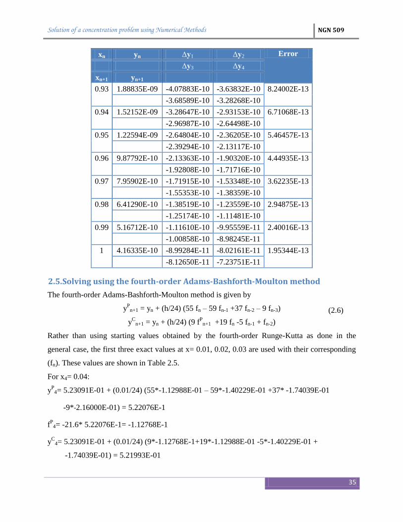
2.5. Solving using the fourth-order Adams-Bashforth-Moulton method
The fourth-order Adams-Bashforth-Moulton method is given by
yP
n+1 = yn + (h/24) (55 fn – 59 fn-1 +37 fn-2 – 9 fn-3)
yC
n+1 = yn + (h/24) (9 fP
n+1 +19 fn -5 fn-1 + fn-2)
Rather than using starting values obtained by the fourth-order Runge-Kutta as done in the
general case, the first three exact values at x= 0.01, 0.02, 0.03 are used with their corresponding
(fn). These values are shown in Table 2.5.
For x4= 0.04:
yP
4= 5.23091E-01 + (0.01/24) (55*-1.12988E-01 – 59*-1.40229E-01 +37* -1.74039E-01
-9*-2.16000E-01) = 5.22076E-1
fP
4= -21.6* 5.22076E-1= -1.12768E-1
yC
4= 5.23091E-01 + (0.01/24) (9*-1.12768E-1+19*-1.12988E-01 -5*-1.40229E-01 +
-1.74039E-01) = 5.21993E-01
(2.6)
Solution of a concentration problem using Numerical Methods NGN 509
36
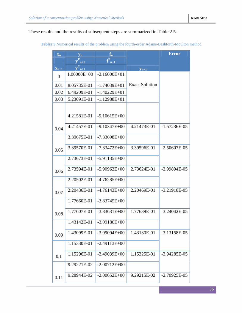
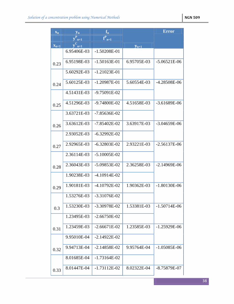
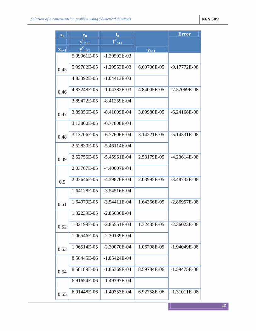
These results and the results of subsequent steps are summarized in Table 2.5.
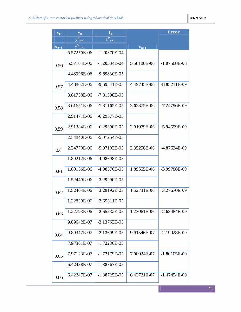
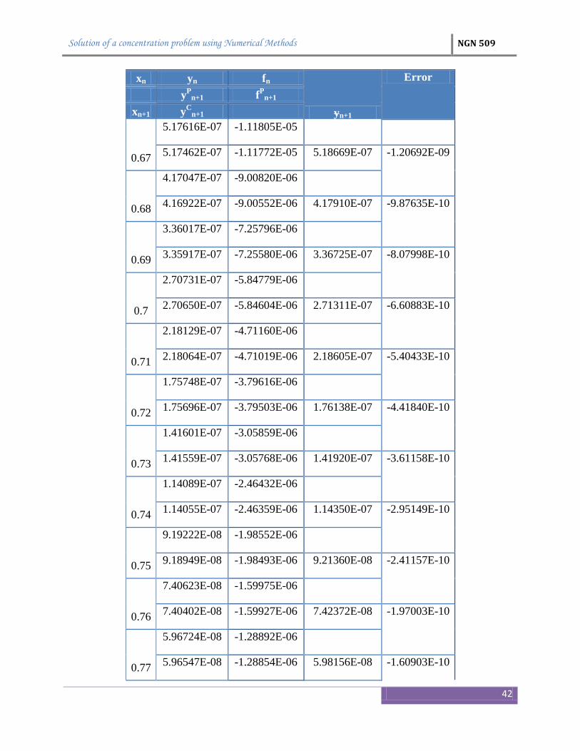
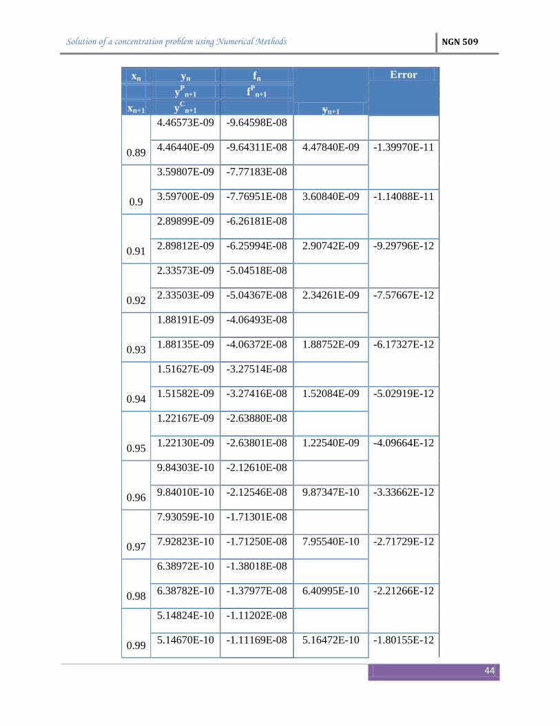
Table2.5 Numerical results of the problem using the fourth-order Adams-Bashforth-Moulton method
xn yn fn
yn+1
Error
yP
n+1 fP
n+1
xn+1 yC
n+1
0 1.00000E+00 -2.16000E+01
Exact Solution
0.01 8.05735E-01 -1.74039E+01
0.02 6.49209E-01 -1.40229E+01
0.03 5.23091E-01 -1.12988E+01
4.21581E-01 -9.10615E+00
0.04 4.21457E-01 -9.10347E+00 4.21473E-01 -1.57236E-05
3.39675E-01 -7.33698E+00
0.05 3.39570E-01 -7.33472E+00 3.39596E-01 -2.50607E-05
2.73673E-01 -5.91135E+00
0.06 2.73594E-01 -5.90963E+00 2.73624E-01 -2.99894E-05
2.20502E-01 -4.76285E+00
0.07 2.20436E-01 -4.76143E+00 2.20469E-01 -3.21918E-05
1.77660E-01 -3.83745E+00
0.08 1.77607E-01 -3.83631E+00 1.77639E-01 -3.24042E-05
1.43142E-01 -3.09186E+00
0.09 1.43099E-01 -3.09094E+00 1.43130E-01 -3.13158E-05
1.15330E-01 -2.49113E+00
0.1 1.15296E-01 -2.49039E+00 1.15325E-01 -2.94285E-05
9.29221E-02 -2.00712E+00
0.11 9.28944E-02 -2.00652E+00 9.29215E-02 -2.70925E-05

Solution of a concentration problem using Numerical Methods NGN 509
37
xn yn fn
yn+1
Error
yP
n+1 fP
n+1
xn+1 yC
n+1
7.48679E-02 -1.61715E+00
0.12 7.48456E-02 -1.61666E+00 7.48701E-02 -2.45533E-05
6.03215E-02 -1.30294E+00
0.13 6.03035E-02 -1.30256E+00 6.03255E-02 -2.19782E-05
4.86014E-02 -1.04979E+00
0.14 4.85869E-02 -1.04948E+00 4.86064E-02 -1.94769E-05
3.91584E-02 -8.45822E-01
0.15 3.91468E-02 -8.45570E-01 3.91639E-02 -1.71180E-05
3.15502E-02 -6.81484E-01
0.16 3.15408E-02 -6.81281E-01 3.15557E-02 -1.49405E-05
2.54202E-02 -5.49076E-01
0.17 2.54126E-02 -5.48912E-01 2.54256E-02 -1.29630E-05
2.04812E-02 -4.42394E-01
0.18 2.04751E-02 -4.42262E-01 2.04863E-02 -1.11899E-05
1.65018E-02 -3.56439E-01
0.19 1.64969E-02 -3.56333E-01 1.65065E-02 -9.61651E-06
1.32956E-02 -2.87185E-01
0.2 1.32917E-02 -2.87100E-01 1.32999E-02 -8.23210E-06
1.07124E-02 -2.31387E-01
0.21 1.07092E-02 -2.31318E-01 1.07162E-02 -7.02266E-06
8.63101E-03 -1.86430E-01
0.22 8.62844E-03 -1.86374E-01 8.63441E-03 -5.97243E-06
Solution of a concentration problem using Numerical Methods NGN 509
38
xn yn fn
yn+1
Error
yP
n+1 fP
n+1
xn+1 yC
n+1
6.95406E-03 -1.50208E-01
0.23 6.95198E-03 -1.50163E-01 6.95705E-03 -5.06521E-06
5.60292E-03 -1.21023E-01
0.24 5.60125E-03 -1.20987E-01 5.60554E-03 -4.28508E-06
4.51431E-03 -9.75091E-02
0.25 4.51296E-03 -9.74800E-02 4.51658E-03 -3.61689E-06
3.63721E-03 -7.85636E-02
0.26 3.63612E-03 -7.85402E-02 3.63917E-03 -3.04659E-06
2.93052E-03 -6.32992E-02
0.27 2.92965E-03 -6.32803E-02 2.93221E-03 -2.56137E-06
2.36114E-03 -5.10005E-02
0.28 2.36043E-03 -5.09853E-02 2.36258E-03 -2.14969E-06
1.90238E-03 -4.10914E-02
0.29 1.90181E-03 -4.10792E-02 1.90362E-03 -1.80130E-06
1.53276E-03 -3.31076E-02
0.3 1.53230E-03 -3.30978E-02 1.53381E-03 -1.50714E-06
1.23495E-03 -2.66750E-02
0.31 1.23459E-03 -2.66671E-02 1.23585E-03 -1.25929E-06
9.95010E-04 -2.14922E-02
0.32 9.94713E-04 -2.14858E-02 9.95764E-04 -1.05085E-06
8.01685E-04 -1.73164E-02
0.33 8.01447E-04 -1.73112E-02 8.02322E-04 -8.75879E-07

Solution of a concentration problem using Numerical Methods NGN 509
39
xn yn fn
yn+1
Error
yP
n+1 fP
n+1
xn+1 yC
n+1
6.45923E-04 -1.39519E-02
0.34 6.45730E-04 -1.39478E-02 6.46460E-04 -7.29228E-07
5.20424E-04 -1.12412E-02
0.35 5.20269E-04 -1.12378E-02 5.20875E-04 -6.06500E-07
4.19309E-04 -9.05707E-03
0.36 4.19184E-04 -9.05437E-03 4.19688E-04 -5.03934E-07
3.37839E-04 -7.29733E-03
0.37 3.37739E-04 -7.29516E-03 3.38157E-04 -4.18330E-07
2.72199E-04 -5.87950E-03
0.38 2.72118E-04 -5.87775E-03 2.72465E-04 -3.46967E-07
2.19313E-04 -4.73715E-03
0.39 2.19247E-04 -4.73574E-03 2.19535E-04 -2.87543E-07
1.76701E-04 -3.81675E-03
0.4 1.76649E-04 -3.81561E-03 1.76887E-04 -2.38112E-07
1.42369E-04 -3.07518E-03
0.41 1.42327E-04 -3.07426E-03 1.42524E-04 -1.97036E-07
1.14708E-04 -2.47769E-03
0.42 1.14674E-04 -2.47695E-03 1.14837E-04 -1.62932E-07
9.24208E-05 -1.99629E-03
0.43 9.23933E-05 -1.99570E-03 9.25279E-05 -1.34643E-07
7.44640E-05 -1.60842E-03
0.44 7.44418E-05 -1.60794E-03 7.45530E-05 -1.11196E-07
Solution of a concentration problem using Numerical Methods NGN 509
40
xn yn fn
yn+1
Error
yP
n+1 fP
n+1
xn+1 yC
n+1
5.99961E-05 -1.29592E-03
0.45 5.99782E-05 -1.29553E-03 6.00700E-05 -9.17772E-08
4.83392E-05 -1.04413E-03
0.46 4.83248E-05 -1.04382E-03 4.84005E-05 -7.57069E-08
3.89472E-05 -8.41259E-04
0.47 3.89356E-05 -8.41009E-04 3.89980E-05 -6.24168E-08
3.13800E-05 -6.77808E-04
0.48 3.13706E-05 -6.77606E-04 3.14221E-05 -5.14331E-08
2.52830E-05 -5.46114E-04
0.49 2.52755E-05 -5.45951E-04 2.53179E-05 -4.23614E-08
2.03707E-05 -4.40007E-04
0.5 2.03646E-05 -4.39876E-04 2.03995E-05 -3.48732E-08
1.64128E-05 -3.54516E-04
0.51 1.64079E-05 -3.54411E-04 1.64366E-05 -2.86957E-08
1.32239E-05 -2.85636E-04
0.52 1.32199E-05 -2.85551E-04 1.32435E-05 -2.36023E-08
1.06546E-05 -2.30139E-04
0.53 1.06514E-05 -2.30070E-04 1.06708E-05 -1.94049E-08
8.58445E-06 -1.85424E-04
0.54 8.58189E-06 -1.85369E-04 8.59784E-06 -1.59475E-08
6.91654E-06 -1.49397E-04
0.55 6.91448E-06 -1.49353E-04 6.92758E-06 -1.31011E-08
Solution of a concentration problem using Numerical Methods NGN 509
41
xn yn fn
yn+1
Error
yP
n+1 fP
n+1
xn+1 yC
n+1
5.57270E-06 -1.20370E-04
0.56 5.57104E-06 -1.20334E-04 5.58180E-06 -1.07588E-08
4.48996E-06 -9.69830E-05
0.57 4.48862E-06 -9.69541E-05 4.49745E-06 -8.83211E-09
3.61758E-06 -7.81398E-05
0.58 3.61651E-06 -7.81165E-05 3.62375E-06 -7.24796E-09
2.91471E-06 -6.29577E-05
0.59 2.91384E-06 -6.29390E-05 2.91979E-06 -5.94599E-09
2.34840E-06 -5.07254E-05
0.6 2.34770E-06 -5.07103E-05 2.35258E-06 -4.87634E-09
1.89212E-06 -4.08698E-05
0.61 1.89156E-06 -4.08576E-05 1.89555E-06 -3.99788E-09
1.52449E-06 -3.29290E-05
0.62 1.52404E-06 -3.29192E-05 1.52731E-06 -3.27670E-09
1.22829E-06 -2.65311E-05
0.63 1.22793E-06 -2.65232E-05 1.23061E-06 -2.68484E-09
9.89642E-07 -2.13763E-05
0.64 9.89347E-07 -2.13699E-05 9.91546E-07 -2.19928E-09
7.97361E-07 -1.72230E-05
0.65 7.97123E-07 -1.72179E-05 7.98924E-07 -1.80105E-09
6.42438E-07 -1.38767E-05
0.66 6.42247E-07 -1.38725E-05 6.43721E-07 -1.47454E-09
Solution of a concentration problem using Numerical Methods NGN 509
42
xn yn fn
yn+1
Error
yP
n+1 fP
n+1
xn+1 yC
n+1
5.17616E-07 -1.11805E-05
0.67 5.17462E-07 -1.11772E-05 5.18669E-07 -1.20692E-09
4.17047E-07 -9.00820E-06
0.68 4.16922E-07 -9.00552E-06 4.17910E-07 -9.87635E-10
3.36017E-07 -7.25796E-06
0.69 3.35917E-07 -7.25580E-06 3.36725E-07 -8.07998E-10
2.70731E-07 -5.84779E-06
0.7 2.70650E-07 -5.84604E-06 2.71311E-07 -6.60883E-10
2.18129E-07 -4.71160E-06
0.71 2.18064E-07 -4.71019E-06 2.18605E-07 -5.40433E-10
1.75748E-07 -3.79616E-06
0.72 1.75696E-07 -3.79503E-06 1.76138E-07 -4.41840E-10
1.41601E-07 -3.05859E-06
0.73 1.41559E-07 -3.05768E-06 1.41920E-07 -3.61158E-10
1.14089E-07 -2.46432E-06
0.74 1.14055E-07 -2.46359E-06 1.14350E-07 -2.95149E-10
9.19222E-08 -1.98552E-06
0.75 9.18949E-08 -1.98493E-06 9.21360E-08 -2.41157E-10
7.40623E-08 -1.59975E-06
0.76 7.40402E-08 -1.59927E-06 7.42372E-08 -1.97003E-10
5.96724E-08 -1.28892E-06
0.77 5.96547E-08 -1.28854E-06 5.98156E-08 -1.60903E-10

Solution of a concentration problem using Numerical Methods NGN 509
43
xn yn fn
yn+1
Error
yP
n+1 fP
n+1
xn+1 yC
n+1
4.80784E-08 -1.03849E-06
0.78 4.80641E-08 -1.03818E-06 4.81955E-08 -1.31395E-10
3.87371E-08 -8.36721E-07
0.79 3.87255E-08 -8.36472E-07 3.88328E-08 -1.07279E-10
3.12107E-08 -6.74151E-07
0.8 3.12014E-08 -6.73950E-07 3.12890E-08 -8.75739E-11
2.51466E-08 -5.43168E-07
0.81 2.51392E-08 -5.43006E-07 2.52106E-08 -7.14764E-11
2.02608E-08 -4.37633E-07
0.82 2.02548E-08 -4.37503E-07 2.03131E-08 -5.83282E-11
1.63243E-08 -3.52604E-07
0.83 1.63194E-08 -3.52499E-07 1.63670E-08 -4.75910E-11
1.31525E-08 -2.84095E-07
0.84 1.31486E-08 -2.84010E-07 1.31875E-08 -3.88243E-11
1.05971E-08 -2.28897E-07
0.85 1.05939E-08 -2.28829E-07 1.06256E-08 -3.16677E-11
8.53814E-09 -1.84424E-07
0.86 8.53559E-09 -1.84369E-07 8.56142E-09 -2.58264E-11
6.87923E-09 -1.48591E-07
0.87 6.87718E-09 -1.48547E-07 6.89824E-09 -2.10595E-11
5.54263E-09 -1.19721E-07
0.88 5.54098E-09 -1.19685E-07 5.55815E-09 -1.71701E-11
Solution of a concentration problem using Numerical Methods NGN 509
44
xn yn fn
yn+1
Error
yP
n+1 fP
n+1
xn+1 yC
n+1
4.46573E-09 -9.64598E-08
0.89 4.46440E-09 -9.64311E-08 4.47840E-09 -1.39970E-11
3.59807E-09 -7.77183E-08
0.9 3.59700E-09 -7.76951E-08 3.60840E-09 -1.14088E-11
2.89899E-09 -6.26181E-08
0.91 2.89812E-09 -6.25994E-08 2.90742E-09 -9.29796E-12
2.33573E-09 -5.04518E-08
0.92 2.33503E-09 -5.04367E-08 2.34261E-09 -7.57667E-12
1.88191E-09 -4.06493E-08
0.93 1.88135E-09 -4.06372E-08 1.88752E-09 -6.17327E-12
1.51627E-09 -3.27514E-08
0.94 1.51582E-09 -3.27416E-08 1.52084E-09 -5.02919E-12
1.22167E-09 -2.63880E-08
0.95 1.22130E-09 -2.63801E-08 1.22540E-09 -4.09664E-12
9.84303E-10 -2.12610E-08
0.96 9.84010E-10 -2.12546E-08 9.87347E-10 -3.33662E-12
7.93059E-10 -1.71301E-08
0.97 7.92823E-10 -1.71250E-08 7.95540E-10 -2.71729E-12
6.38972E-10 -1.38018E-08
0.98 6.38782E-10 -1.37977E-08 6.40995E-10 -2.21266E-12
5.14824E-10 -1.11202E-08
0.99 5.14670E-10 -1.11169E-08 5.16472E-10 -1.80155E-12

Solution of a concentration problem using Numerical Methods NGN 509
45
xn yn fn
yn+1
Error
yP
n+1 fP
n+1
xn+1 yC
n+1
4.14797E-10 -8.95961E-09
1 4.14673E-10 -8.95694E-09 4.16140E-10 -1.4667E-12

Solution of a concentration problem using Numerical Methods NGN 509
46
Solution of a concentration problem using Numerical Methods NGN 509
47
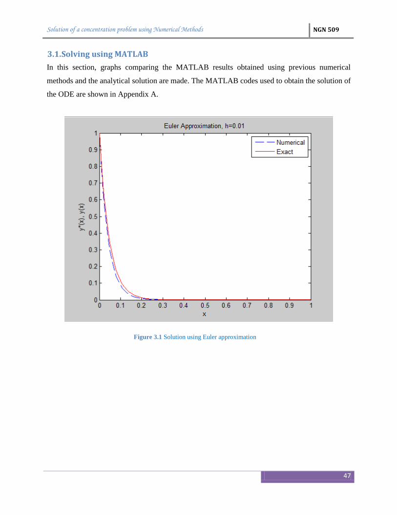
3.1. Solving using MATLAB
In this section, graphs comparing the MATLAB results obtained using previous numerical
methods and the analytical solution are made. The MATLAB codes used to obtain the solution of
the ODE are shown in Appendix A.
Figure 3.1 Solution using Euler approximation
Solution of a concentration problem using Numerical Methods NGN 509
48
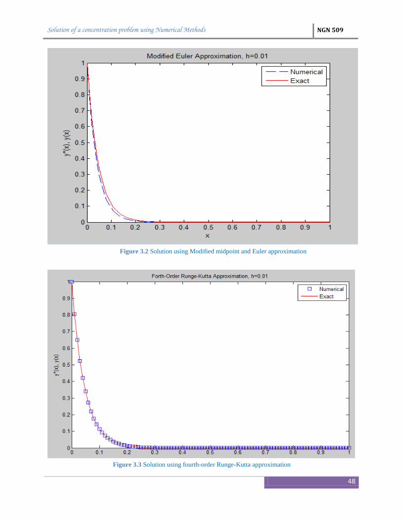
Figure 3.2 Solution using Modified midpoint and Euler approximation
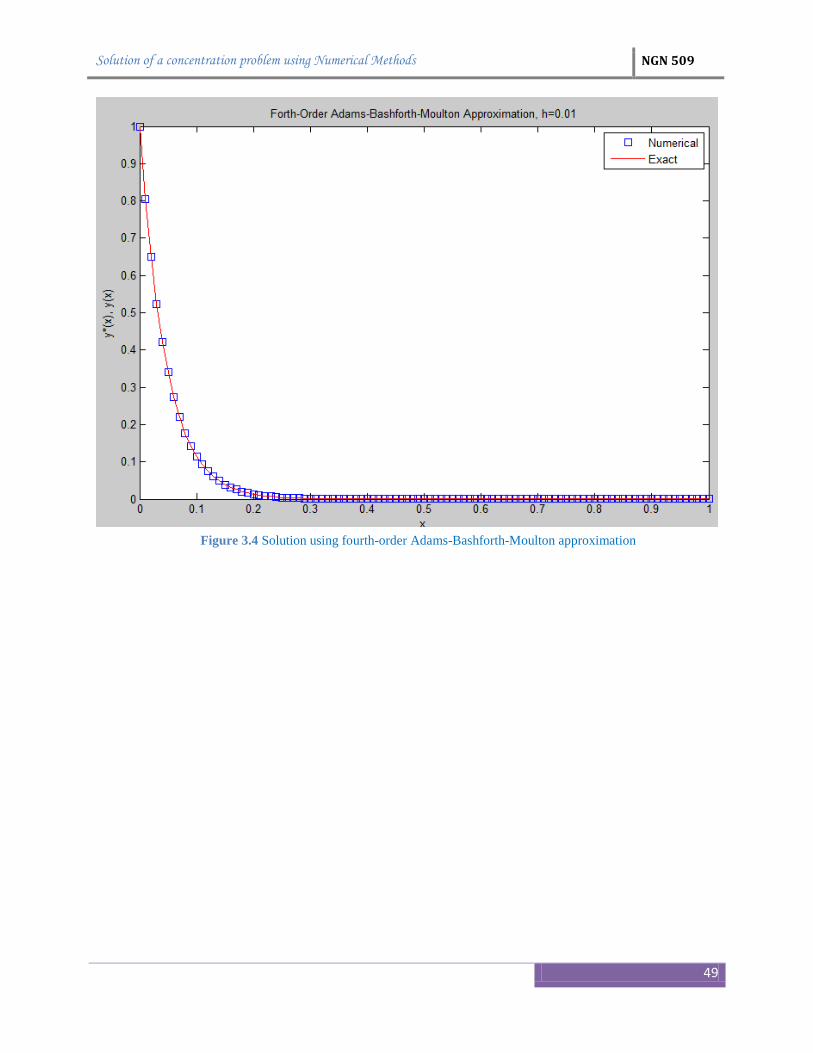
Figure 3.3 Solution using fourth-order Runge-Kutta approximation
Solution of a concentration problem using Numerical Methods NGN 509
49
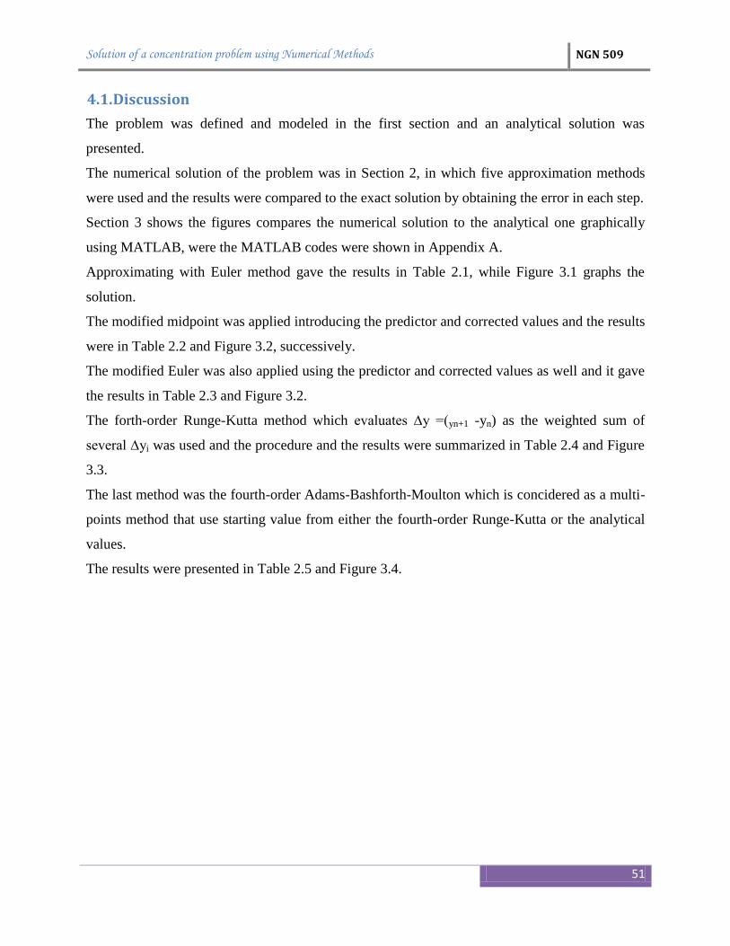
Figure 3.4 Solution using fourth-order Adams-Bashforth-Moulton approximation

Solution of a concentration problem using Numerical Methods NGN 509
50
Solution of a concentration problem using Numerical Methods NGN 509
51
4.1. Discussion
The problem was defined and modeled in the first section and an analytical solution was
presented.
The numerical solution of the problem was in Section 2, in which five approximation methods
were used and the results were compared to the exact solution by obtaining the error in each step.
Section 3 shows the figures compares the numerical solution to the analytical one graphically
using MATLAB, were the MATLAB codes were shown in Appendix A.
Approximating with Euler method gave the results in Table 2.1, while Figure 3.1 graphs the
solution.
The modified midpoint was applied introducing the predictor and corrected values and the results
were in Table 2.2 and Figure 3.2, successively.
The modified Euler was also applied using the predictor and corrected values as well and it gave
the results in Table 2.3 and Figure 3.2.
The forth-order Runge-Kutta method which evaluates ∆y =(yn+1 -yn) as the weighted sum of
several ∆yi was used and the procedure and the results were summarized in Table 2.4 and Figure
3.3.
The last method was the fourth-order Adams-Bashforth-Moulton which is concidered as a multi-
points method that use starting value from either the fourth-order Runge-Kutta or the analytical
values.
The results were presented in Table 2.5 and Figure 3.4.
Solution of a concentration problem using Numerical Methods NGN 509
52
5.1. Conclusion
Most of the problems in the engineering field can be explained in a way that gives an analytical
solution, but most of the times it’s complicated and might take long time to solve.
Numerical methods are used as fast ways that offer approximate solutions which are simple to
obtain and have accuracy that is good enough and close to the exact solution.
For the aim of this project, four single-point methods and one multi-points method were used.
The first, the fastest and the simplest was the 1st order Explicit Euler Method.
This method relatively has low accuracy but this was modified using a small step size. The
importance of small step size is extreme in this method as the solution might diverge if the step
was large as the method is conditionally stable.
The limit of stability for this method is [-1 ]. The right-hand inequality is
always satisfied for (21h 1), while the left-hand side is satisfied only if h 0.095 (or 21h 2).
The second numerical method used was the modified midpoint method which is considered as a
second order single-point method.
The errors presented in Table 2.2 for the second-order modified midpoint method are
approximately1 5 times smaller than the errors presented in Table 2.1 for the first-order explicit
Euler method. This illustrates the advantage of the second-order method.
The third method used was the modified Euler method which is considered as an alternate
approach for solving the implicit midpoint FDE.
Both, the modified midpoint and the modified Euler methods have a limit of stability of (21h 2)
or (h 0.095) which is the same as the first-order Euler method.
The fourth-order Runge-Kutta method is one ne of the most popular method of the Runge-Kutta
family. It gave the most accurate results with extremely small error as described in Table 2.4 and
Figure 3.3.
The stability condition for this method is
G = 1 + 21 h + 0.5 ( -21 h)2 – (1/6)*(-21h)
3 + (1/24) (-21h)
4
This implies that |G| 1 if (21h 2.785), where G = yn+1/yn.
Last method applied was the fourth-order Adams-Bashforth-Moulton method as an example of
the multi-points methods.
Comparing the results in Table 2.5 obtained using this method to the results in Table 2.4
obtained using the fourth-order Runge-Kutta method shows how different they are regarding the
(5.1)

Solution of a concentration problem using Numerical Methods NGN 509
53
errors. For example, at x=1, Table 2.4 gives an error of 1.95344E-13 which is approximately 8
times smaller than the corresponding error in Table 2.5. However, the Runge-Kutta method
requires four derivative function evaluations per step compared to two for the Adams-Bashforth-
Moulton method.
The stability condition for this method is
(
)
For stability, the whole for roots of G should be 1. Solving this equation gives the results
shown in Figure 5.1 [7]
In this project, the method is stable as (21h= 0.21) gives G 1.
(5.2)
Figure 5.1 Solution of equation (5.2)

Solution of a concentration problem using Numerical Methods NGN 509
54
Solution of a concentration problem using Numerical Methods NGN 509
55
References
[1] Kehoe, J. P. G. and J. B. Butt,(1972), "Interactions of Inter- and. Intraphase. Gradients in a
Diffusion Limited Catalytic Reaction," A.I.Ch.E. J., 18, 347
[2] Price. T. H, Gradients in a Diffusion Liniiteci Catalytic Reaction,” A.I.Ch.E. J., 18, 347, and
J. B. Butt, “Catalyst Poisoning and Fixed Bed Reactor Dynamics-TI.” Chern. Eng, Sci., 32, 393,
(1977).
[3] http://chemelab.ucsd.edu/CAPE/tutorial/aspentutorial01.pdf, cited on January 2013
[4] S.B. Halligudi*, H.C. Bajaj, K.N. Bhatt and M. Krishnaratnam, Hydrogenation of Benzene to
Cyclohexane Catalyzed by Rhodium(I) Complex Supported on Montmorillonite Clay, Central
Salt and Marine Chemicals Research Institute, Bhavnagar 364 002, India, September 1992
[5] John K. Marangozis , Basil G. Mantzouranls , Anastasios N. Sophos, Intrinsic Kinetics of
Hydrogenation of Benzene on Nickel Catalysts Supported on Kieselguhr, March 1979
[6] K. M. M. Al-Abrahemee, Solution of Some Application of System of Ordinary Initial Value
Problems Using Osculatory Interpolation Technique, Department of Mathematics, College of
Education ,University of Al- Qadysea, December 2011
[7] Joe D. Hoffman, Numerical Methods for Engineers and Scientists, Second Edition, 2001
Solution of a concentration problem using Numerical Methods NGN 509
56
APPENDIX A
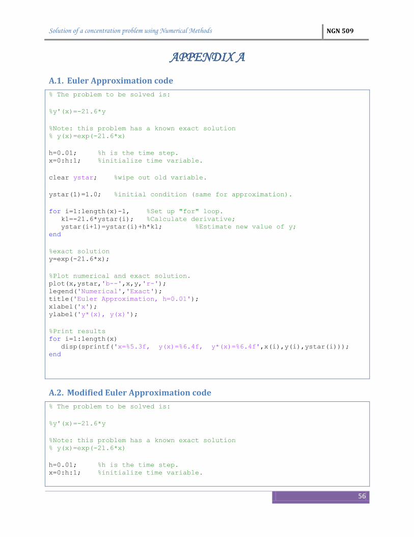
A.1. Euler Approximation code
% The problem to be solved is:
%y'(x)=-21.6*y
%Note: this problem has a known exact solution % y(x)=exp(-21.6*x)
h=0.01; %h is the time step. x=0:h:1; %initialize time variable.
clear ystar; %wipe out old variable.
ystar(1)=1.0; %initial condition (same for approximation).
for i=1:length(x)-1, %Set up "for" loop. k1=-21.6*ystar(i); %Calculate derivative; ystar(i+1)=ystar(i)+h*k1; %Estimate new value of y; end
%exact solution y=exp(-21.6*x);
%Plot numerical and exact solution. plot(x,ystar,'b--',x,y,'r-'); legend('Numerical','Exact'); title('Euler Approximation, h=0.01'); xlabel('x'); ylabel('y*(x), y(x)');
%Print results for i=1:length(x) disp(sprintf('x=%5.3f, y(x)=%6.4f, y*(x)=%6.4f',x(i),y(i),ystar(i))); end
A.2. Modified Euler Approximation code
% The problem to be solved is:
%y'(x)=-21.6*y
%Note: this problem has a known exact solution % y(x)=exp(-21.6*x)
h=0.01; %h is the time step. x=0:h:1; %initialize time variable.
Solution of a concentration problem using Numerical Methods NGN 509
57
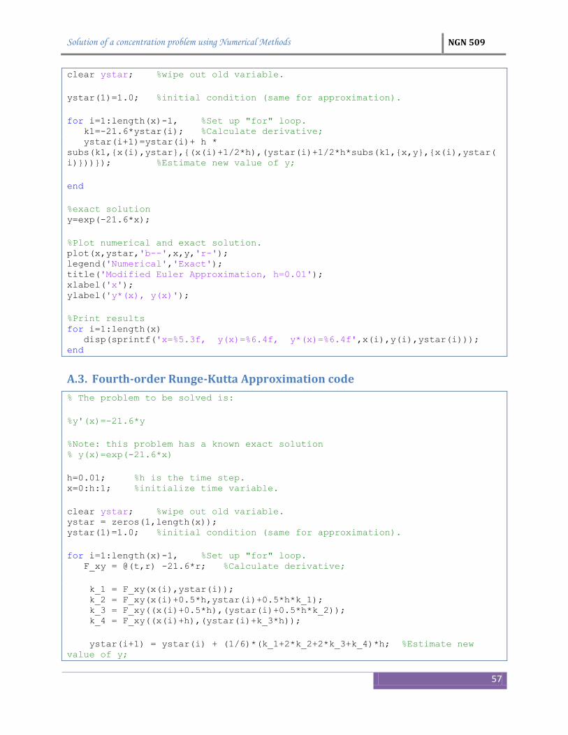
clear ystar; %wipe out old variable.
ystar(1)=1.0; %initial condition (same for approximation).
for i=1:length(x)-1, %Set up "for" loop. k1=-21.6*ystar(i); %Calculate derivative; ystar(i+1)=ystar(i)+ h *
subs(k1,{x(i),ystar},{(x(i)+1/2*h),(ystar(i)+1/2*h*subs(k1,{x,y},{x(i),ystar(
i)}))}); %Estimate new value of y;
end
%exact solution y=exp(-21.6*x);
%Plot numerical and exact solution. plot(x,ystar,'b--',x,y,'r-'); legend('Numerical','Exact'); title('Modified Euler Approximation, h=0.01'); xlabel('x'); ylabel('y*(x), y(x)');
%Print results for i=1:length(x) disp(sprintf('x=%5.3f, y(x)=%6.4f, y*(x)=%6.4f',x(i),y(i),ystar(i))); end
A.3. Fourth-order Runge-Kutta Approximation code
% The problem to be solved is:
%y'(x)=-21.6*y
%Note: this problem has a known exact solution % y(x)=exp(-21.6*x)
h=0.01; %h is the time step. x=0:h:1; %initialize time variable.
clear ystar; %wipe out old variable. ystar = zeros(1,length(x)); ystar(1)=1.0; %initial condition (same for approximation).
for i=1:length(x)-1, %Set up "for" loop. F_xy = @(t,r) -21.6*r; %Calculate derivative;
k_1 = F_xy(x(i),ystar(i)); k_2 = F_xy(x(i)+0.5*h,ystar(i)+0.5*h*k_1); k_3 = F_xy((x(i)+0.5*h),(ystar(i)+0.5*h*k_2)); k_4 = F_xy((x(i)+h),(ystar(i)+k_3*h));
ystar(i+1) = ystar(i) + (1/6)*(k_1+2*k_2+2*k_3+k_4)*h; %Estimate new
value of y;
Solution of a concentration problem using Numerical Methods NGN 509
58
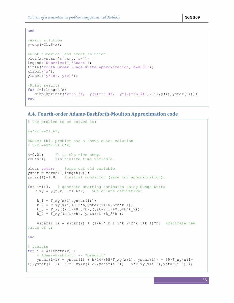
end
%exact solution y=exp(-21.6*x);
%Plot numerical and exact solution. plot(x,ystar,'s',x,y,'r-'); legend('Numerical','Exact'); title('Forth-Order Runge-Kutta Approximation, h=0.01'); xlabel('x'); ylabel('y*(x), y(x)');
%Print results for i=1:length(x) disp(sprintf('x=%5.3f, y(x)=%6.4f, y*(x)=%6.4f',x(i),y(i),ystar(i))); end
A.4. Fourth-order Adams-Bashforth-Moulton Approximation code
% The problem to be solved is:
%y'(x)=-21.6*y
%Note: this problem has a known exact solution % y(x)=exp(-21.6*x)
h=0.01; %h is the time step. x=0:h:1; %initialize time variable.
clear ystar; %wipe out old variable. ystar = zeros(1,length(x)); ystar(1)=1.0; %initial condition (same for approximation).
for i=1:3, % generate starting estimates using Runge-Kutta F_xy = @(t,r) -21.6*r; %Calculate derivative;
k_1 = F_xy(x(i),ystar(i)); k_2 = F_xy(x(i)+0.5*h,ystar(i)+0.5*h*k_1); k_3 = F_xy((x(i)+0.5*h),(ystar(i)+0.5*h*k_2)); k_4 = F_xy((x(i)+h),(ystar(i)+k_3*h));
ystar(i+1) = ystar(i) + (1/6)*(k_1+2*k_2+2*k_3+k_4)*h; %Estimate new
value of y;
end
% iterate for i = 4:length(x)-1 % Adams-Bashforth -- *predict* ystar(i+1) = ystar(i) + h/24*(55*F_xy(x(i), ystar(i)) - 59*F_xy(x(i-
1),ystar(i-1))+ 37*F_xy(x(i-2),ystar(i-2)) - 9*F_xy(x(i-3),ystar(i-3)));
Solution of a concentration problem using Numerical Methods NGN 509
59
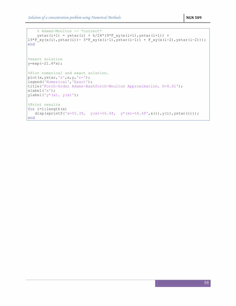
% Adams-Moulton -- *correct* ystar(i+1) = ystar(i) + h/24*(9*F_xy(x(i+1),ystar(i+1)) +
19*F_xy(x(i),ystar(i))- 5*F_xy(x(i-1),ystar(i-1)) + F_xy(x(i-2),ystar(i-2))); end
%exact solution y=exp(-21.6*x);
%Plot numerical and exact solution. plot(x,ystar,'s',x,y,'r-'); legend('Numerical','Exact'); title('Forth-Order Adams-Bashforth-Moulton Approximation, h=0.01'); xlabel('x'); ylabel('y*(x), y(x)');
%Print results for i=1:length(x) disp(sprintf('x=%5.3f, y(x)=%6.4f, y*(x)=%6.4f',x(i),y(i),ystar(i))); end