solar euv and xuv energy input to thermosphere on solar rotation time scales derived from...

Solar EUV and XUV energy input to thermosphere on solarrotation time scales derived from photoelectron observations

W. K. Peterson,1 T. N. Woods,1 J. M. Fontenla,1 P. G. Richards,2 P. C. Chamberlin,3

S. C. Solomon,4 W. K. Tobiska,5 and H. P. Warren6

Received 17 November 2011; revised 27 February 2012; accepted 5 April 2012; published 18 May 2012.

[1] Solar radiation below �100 nm produces photoelectrons, a substantial portion of theF region ionization, most of the E region ionization, and drives chemical reactions in thethermosphere. Unquantified uncertainties in thermospheric models exist because ofuncertainties in solar irradiance models used to fill spectral and temporal gaps in solarirradiance observations. We investigate uncertainties in solar energy input to thethermosphere on solar rotation time scales using photoelectron observations from theFAST satellite. We compare observed and modeled photoelectron energy spectra using twophotoelectron production codes driven by five different solar irradiance models. Weobserve about 1.7% of the ionizing solar irradiance power in the escaping photoelectronflux. Most of the code/model pairs used reproduce the average escaping photoelectron fluxover a 109-day interval in late 2006. The code/model pairs we used do not completelyreproduce the observed spectral and solar rotation variations in photoelectron powerdensity. For the interval examined, 30% of the variability in photoelectron power densitywith equivalent wavelengths between 18 and 45 nm was not captured in the code/modelpairs. For equivalent wavelengths below �16 nm, most of the variability was missed.This result implies that thermospheric model runs based on the solar irradiance models wetested systematically underestimate the energy input from ionizing radiation on solarrotation time scales.

Citation: Peterson, W. K., T. N. Woods, J. M. Fontenla, P. G. Richards, P. C. Chamberlin, S. C. Solomon, W. K. Tobiska, andH. P. Warren (2012), Solar EUV and XUV energy input to thermosphere on solar rotation time scales derived from photoelectronobservations, J. Geophys. Res., 117, A05320, doi:10.1029/2011JA017382.

1. Introduction

[2] The Earth’s thermosphere is heated primarily by solarradiation. Extensive model runs of large-scale, community-based, thermospheric general circulation models are now thebest way to interpret how changes in energy inputs fromsolar irradiance, Joule heating, and particle precipitation aredistributed to the thermosphere during periods of solar andgeomagnetic activity. However, the quantitative limitations,

and therefore usefulness of these models, on solar rotationtime scales remains to be determined. Here we presentphotoelectron observations for 109 days in late 2006, nearthe end of solar cycle 23. We use solar irradiance models andphotoelectron production codes to evaluate the uncertaintyin energy input to the thermosphere associated with uncer-tainties in photochemical models and in the spectral andtemporal variability of solar irradiance on solar rotation timescales.[3] There has been continual improvement in both the

spectral and temporal resolution of solar irradiance observa-tions over the years, but only since the launch of NASA’sSolar Dynamics Observatory (SDO) have the high temporal,high spectral resolution observations of solar irradiance atwavelengths between �1 and �100 nm necessary for aero-nomic calculations become available [Woods et al., 2010].To fill the historical spectral and temporal gaps in ourknowledge of solar EUV and XUV observations, empirical,first principles, and observation driven solar irradiancemodels have been developed. These models are neededespecially for the ionizing wavelengths below�45 nm wheresolar EUV and XUV radiation is most variable. As shownbelow, the spectral character of solar irradiance models differsignificantly from each other and available observations.

1Laboratory for Atmospheric and Space Physics, University ofColorado at Boulder, Boulder, Colorado, USA.

2Physics Department, George Mason University, Fairfax, Virginia,USA.

3NASA Goddard Space Flight Center, Greenbelt, Maryland, USA.4High Altitude Observatory, National Center for Atmospheric Research,

Boulder, Colorado, USA.5Space Weather Center, Utah State University, Logan, Utah, USA.6Space Science Division, Naval Research Laboratory, Washington, DC,

USA.

Corresponding author: W. K. Peterson, Laboratory for Atmospheric andSpace Physics, University of Colorado at Boulder, Boulder, CO 80303,USA. ([email protected])

Copyright 2012 by the American Geophysical Union.0148-0227/12/2011JA017382

JOURNAL OF GEOPHYSICAL RESEARCH, VOL. 117, A05320, doi:10.1029/2011JA017382, 2012

A05320 1 of 18

http://dx.doi.org/10.1029/2011JA017382

[4] Photoelectrons are efficiently and immediately pro-duced. They have been used as an indicator of the varyingintensity of solar ionizing radiation for many years [e.g.,Dalgarno et al., 1973]. This study relies on the photoelec-tron observations from the Fast Auroral Snapshot (FAST)satellite [Carlson et al., 2001] to provide the measurementsto which model calculations are compared. Previous com-parisons have been made between FAST photoelectronobservations and calculated photoelectron energy spectraduring two solar flares [Woods et al., 2003; Peterson et al.,2008] and for three days with minimal solar activity in2002, 2003, and 2008 [Peterson et al., 2009]. Peterson et al.[2008] demonstrated that, on solar flare time scales, theuncertainties in photoelectron observations and the FlareIrradiance Spectral Model (FISM) [Chamberlin et al., 2007,2008] were comparable for ionizing radiation below 45 nm.Peterson et al. [2009] found the largest differences betweenobserved and modeled fluxes are in the 4–10 nm range,where photoelectron data from the FAST satellite indicatethat the Thermosphere, Ionosphere, Mesosphere, Energetics,and Dynamics (TIMED) / Solar Extreme Ultraviolet Exper-iment (SEE) Version 9 irradiances are systematically low.Their analysis also suggested that variation on solar cycletimescales in the TIMED/SEE Version 9 data and the FISMirradiance derived from them are systematically low in the18–27 nm range. This paper examines variability on solarrotation time scales using daily average photoelectron fluxesacquired from FAST during the period of September 14th toDecember 31st, 2006 and compares them to photoelectronfluxes calculated from combinations of two photoelectronproduction codes and five solar irradiance models.

[5] Photoelectron observations were made from the FASTsatellite from 1997 to 2008. We use data acquired at altitudesabove 1500 km equatorward of the auroral oval. The paper isorganized as follows. We briefly discuss the technique, solarirradiance observations, irradiance models, and photoelec-tron production codes. We present daily averaged observedphotoelectron fluxes and those calculated from the suite ofcode/irradiance model pairs for the last 109 days in 2006.The calculated and observed photoelectron data are com-pared in multiple formats to explore the spatial and spectralvariability of the photoelectron power density on solarrotation time scales as well as over the entire interval.Finally, the implications of the comparisons on the reliabilityof solar irradiance models in the 2–45 nm range on solarrotation time scales are discussed.

2. Photoelectron Observations

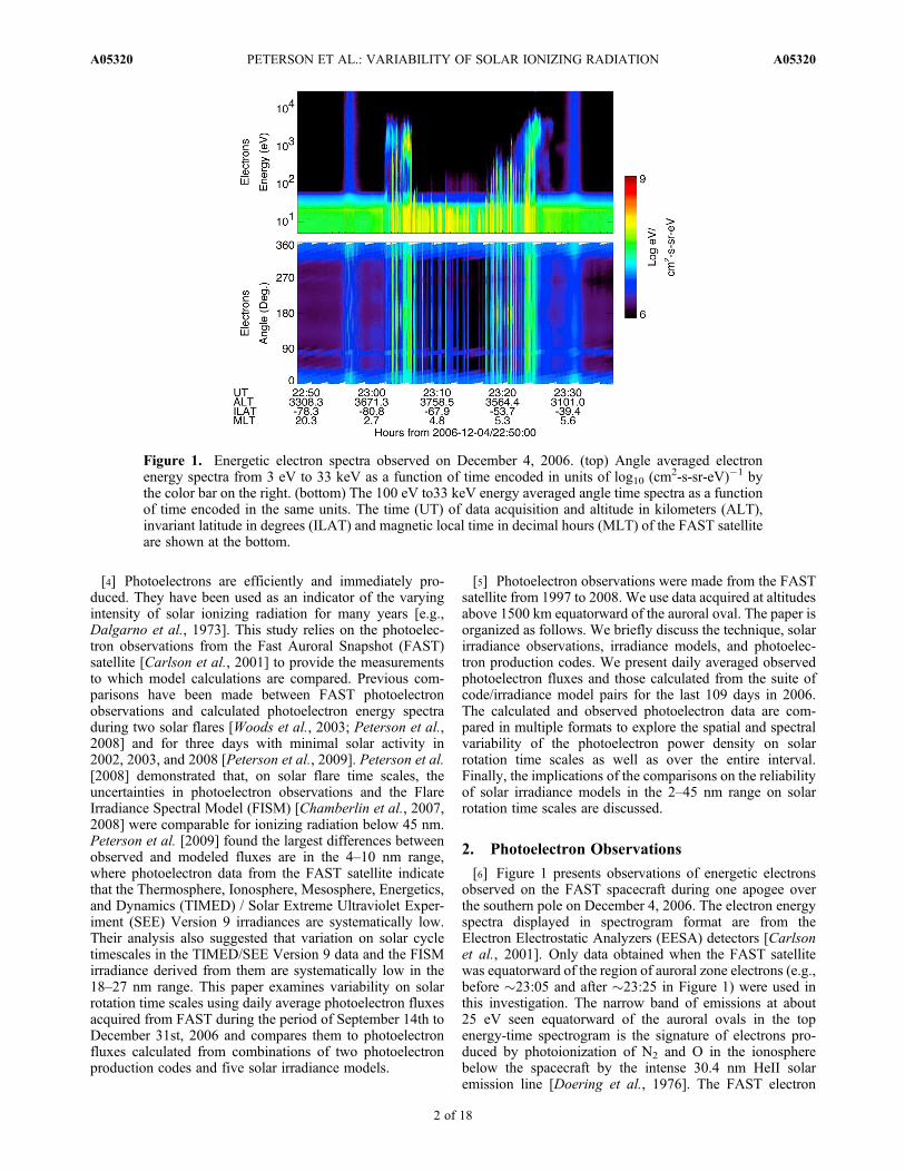
[6] Figure 1 presents observations of energetic electronsobserved on the FAST spacecraft during one apogee overthe southern pole on December 4, 2006. The electron energyspectra displayed in spectrogram format are from theElectron Electrostatic Analyzers (EESA) detectors [Carlsonet al., 2001]. Only data obtained when the FAST satellitewas equatorward of the region of auroral zone electrons (e.g.,before �23:05 and after �23:25 in Figure 1) were used inthis investigation. The narrow band of emissions at about25 eV seen equatorward of the auroral ovals in the topenergy-time spectrogram is the signature of electrons pro-duced by photoionization of N2 and O in the ionospherebelow the spacecraft by the intense 30.4 nm HeII solaremission line [Doering et al., 1976]. The FAST electron

Figure 1. Energetic electron spectra observed on December 4, 2006. (top) Angle averaged electronenergy spectra from 3 eV to 33 keV as a function of time encoded in units of log10 (cm

2-s-sr-eV)�1 bythe color bar on the right. (bottom) The 100 eV to33 keV energy averaged angle time spectra as a functionof time encoded in the same units. The time (UT) of data acquisition and altitude in kilometers (ALT),invariant latitude in degrees (ILAT) and magnetic local time in decimal hours (MLT) of the FAST satelliteare shown at the bottom.

PETERSON ET AL.: VARIABILITY OF SOLAR IONIZING RADIATION A05320A05320

2 of 18

spectrometer has a 360� field of view that includes themagnetic field direction. The instrument samples all pitchangles simultaneously. The energy-averaged pitch anglespectra in Figure 1 (bottom) show several horizontal bands.Electron pitch angles in the range 0–180� are related to theangle shown as follows: From 0 to 180� pitch angle equalsthe angle shown; from 180 to 360� pitch angle equals 360minus the angle shown. The widest and most intense band isnear angles of 0 or 360 degrees, which corresponds to ener-getic photoelectrons coming up field lines from their sourcein the southern hemisphere ionosphere. The width of theband of upflowing photoelectrons is determined by the rela-tive strengths of the magnetic field at the satellite and at thetop of the ionosphere. The two narrower horizontal bandsnear angles of 90� and 270� are produced by photoelectronsgenerated on spacecraft surfaces that are directed to theelectron detectors as they circle the local magnetic field afterthey are produced. The weak horizontal band appearing near180� corresponds to down flowing electrons in the southernhemisphere. These bands are the backscattered photoelec-trons that are generated in the dark magnetically conjugatenorthern hemisphere from the photoelectrons that areobserved streaming up from the sunlit southern hemisphere[Richards and Peterson, 2008]. Penetrating radiation in thering current introduces a background signal independent ofenergy and angle as seen at �22:57 and �23:30 in Figure 1.

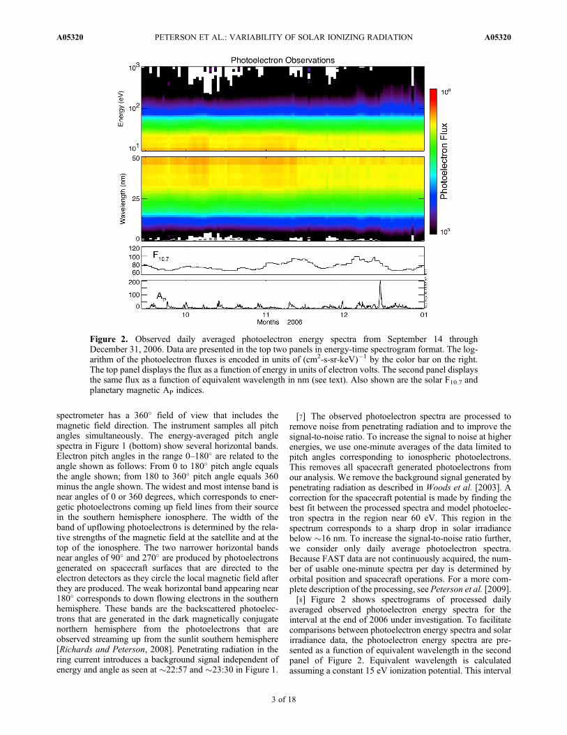
[7] The observed photoelectron spectra are processed toremove noise from penetrating radiation and to improve thesignal-to-noise ratio. To increase the signal to noise at higherenergies, we use one-minute averages of the data limited topitch angles corresponding to ionospheric photoelectrons.This removes all spacecraft generated photoelectrons fromour analysis. We remove the background signal generated bypenetrating radiation as described in Woods et al. [2003]. Acorrection for the spacecraft potential is made by finding thebest fit between the processed spectra and model photoelec-tron spectra in the region near 60 eV. This region in thespectrum corresponds to a sharp drop in solar irradiancebelow �16 nm. To increase the signal-to-noise ratio further,we consider only daily average photoelectron spectra.Because FAST data are not continuously acquired, the num-ber of usable one-minute spectra per day is determined byorbital position and spacecraft operations. For a more com-plete description of the processing, see Peterson et al. [2009].[8] Figure 2 shows spectrograms of processed daily

averaged observed photoelectron energy spectra for theinterval at the end of 2006 under investigation. To facilitatecomparisons between photoelectron energy spectra and solarirradiance data, the photoelectron energy spectra are pre-sented as a function of equivalent wavelength in the secondpanel of Figure 2. Equivalent wavelength is calculatedassuming a constant 15 eV ionization potential. This interval

Figure 2. Observed daily averaged photoelectron energy spectra from September 14 throughDecember 31, 2006. Data are presented in the top two panels in energy-time spectrogram format. The log-arithm of the photoelectron fluxes is encoded in units of (cm2-s-sr-keV)�1 by the color bar on the right.The top panel displays the flux as a function of energy in units of electron volts. The second panel displaysthe same flux as a function of equivalent wavelength in nm (see text). Also shown are the solar F10.7 andplanetary magnetic AP indices.


3 of 18

has modest solar activity as indicated by the F10.7 index andfour X class flares in December. Because of the precessionof the FAST orbit, data are primarily from the northernhemisphere before November 7 and from the southernhemisphere after. Also after November 7 most of the datawere acquired near the terminator where the solar zenithangle was near to but less than 90�. This interval was alsonoteworthy for the recurring low-level geomagnetic activitydriven by variations in the solar wind speed as seen in the AP

index and discussed by Thayer et al. [2008] and others.Variations of the photoelectron energy spectra over solarrotational periods are not prominent in the logarithmicintensity scale used in Figure 2. They are readily apparenthowever in the differential analysis presented below.

3. Solar Irradiance Observations and Models

[9] Only a very small fraction of solar irradiance producesphotoelectrons. Figure 3 presents line plots of total andrepresentative band restricted solar irradiance observationsduring the interval shown in Figure 2. Total solar irradianceincident on Earth observed on the SORCE satellite variedfrom 1345.1423 � 0.5169 W/m2 on September 14 to1407.6471 � 0.4961 W/m2 on December 31, 2006 as theEarth-Sun distance decreased [Kopp and Lean, 2011]. Theband restricted data presented in Figure 3 and the rest of the

paper have been adjusted to constant 1 astronomical unit(AU) values. During this interval, 1 nm resolution irradiancemeasurements above 27 nm were available from the SolarEUV Experiment (SEE) instrument on the ThermosphereIonosphere Mesosphere Energetics and Dynamics (TIMED)Satellite [Woods et al., 1998]. Below 27 nm, broadbandirradiance observations are available from TIMED/SEE andan instrument on the NOAA/GOES series of satellites[Garcia, 1994]. Shown in Figure 3 are 1 nm resolutionirradiances including the Lyman alpha (121.6 nm) and HeII(30.4 nm) lines as well as data from the 0.1–7 nm TIMED/SEE and 0.1–0.8 nm GOES sensors. Also presented inFigure 3 are the integrated irradiance from 27 to 45 nmobtained from TIMED/SEE observations. There is no com-plete spectral coverage of the region below 27 nm for thetime interval of interest. Systematic high-resolution (0.1–1 nm) solar irradiance data from 6 to 27 nm only becameavailable with the launch of the EUV Variability Experiment(EVE) on the Solar Dynamics Observatory (SDO) in Feb-ruary 2010 [Woods et al., 2010].[10] Photoelectrons are directly produced by EUV radia-

tion at wavelengths less than �100 nm. However, photo-electrons with equivalent wavelengths shorter than �35 nmare overwhelmed by secondary photoelectrons produced byhigher energy photoelectrons. About half of the ionizingradiation power occurs below 27 nm where measurements,

Figure 3. Daily average values of observed total and partial solar irradiance for the interval from Sep-tember 14 to December 31, 2006 from the SORCE, TIMED, and GOES satellites in units of W/m2.See text.


4 of 18

prior to those made by SDO/EVE, have inadequate coverageand wavelength resolution to use in models of the interactionof solar radiation with the thermosphere [see, e.g., Petersonet al., 2009]. To provide high spectral resolution solar irra-diance values for use in aeronomical calculations severalsolar irradiance models have been developed to fill spectraland temporal gaps in the observations. Here we considersome of the generally used models including EUVAC[Richards et al., 1994] and its higher spectral resolution

version HEUVAC [Richards et al., 2006], The Flare Irradi-ance Spectral Model (FISM) [Chamberlin et al., 2007, 2008],Solar 2000 (S2000 v2.35 [Tobiska et al., 2008], http://www.spacewx.com/solar2000.html), the Naval Research Labora-tory EUV model (NRLEUV) [Warren, 2006], and the SolarRadiation Physical Model (SRPM) [Fontenla et al., 2009a,2009b, 2011] driven by observations from the Mauna LoaSolar Observatory (MLSO) and the Solar observatory inRome. The SRPM model has an adjustable parameter to

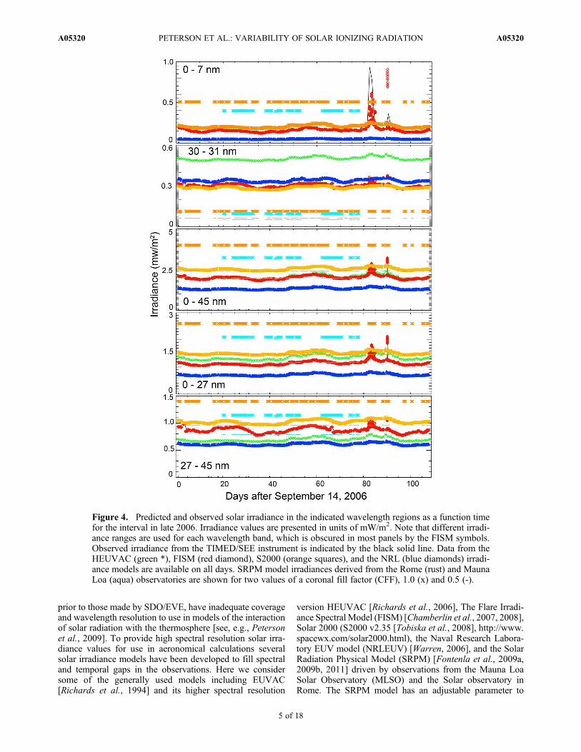
Figure 4. Predicted and observed solar irradiance in the indicated wavelength regions as a function timefor the interval in late 2006. Irradiance values are presented in units of mW/m2. Note that different irradi-ance ranges are used for each wavelength band, which is obscured in most panels by the FISM symbols.Observed irradiance from the TIMED/SEE instrument is indicated by the black solid line. Data from theHEUVAC (green *), FISM (red diamond), S2000 (orange squares), and the NRL (blue diamonds) irradi-ance models are available on all days. SRPM model irradiances derived from the Rome (rust) and MaunaLoa (aqua) observatories are shown for two values of a coronal fill factor (CFF), 1.0 (x) and 0.5 (-).


5 of 18

account for uncertainties associated with modeling coronalemissions using the visible images from the MLSO or Romeobservatories. Here we have used SRPM coronal fillingfactors (CFF) of 1 and 0.5. The HEUVAC and NRLEUVmodels are driven by the F10.7 index; the FISM and S2000models are driven by TIMED/SEE, and GOES X-rayobservations and F10.7 when these observations are notavailable.[11] Comparison of observed photoelectron energy spectra

and solar irradiance models is facilitated by consideringbroad wavelength bands [Peterson et al., 2009]. Figure 4presents model estimated and observed solar irradiancesfor the 0–7, 30–31, 0–45, 0–27, and 27–45 nm ranges.Measurements from the TIMED/SEE instrument are indi-cated by the solid black line in each panel. Model data areindicated by the symbols listed in the caption to Figure 4. Inmany cases the black line is not visible because it is identicalto the FISM model and over-plotted by red diamonds. Asshown in Figure 4, SRPM irradiances generated with a CFFof 0.5 are lower at all wavelengths than those generated witha CFF of 1. We note that the NRL solar irradiance modeldoes not extend below 5 nm [Warren, 2006], accounting forthe low value for the NRL irradiance over the 0–7 nm regiongiven in Figure 4 (top).[12] The two relatively short intervals of solar activity

centered on December 6 and 12 (days 83 and 89 in Figure 4)shown in the TIMED/SEE data are associated with bursts ofsolar flares. We note the significant spectral differences of theirradiance models displayed in Figure 4 and calculated pho-toelectron spectra shown in Figure 5. The goal of this paper isto compare, on solar rotation time scales, observed photo-electron energy spectra with those calculated using the vari-ous solar irradiance models. Before we do the comparison,

we first need to describe the photoelectron production codeswe are using in more detail.

4. Photoelectron Models

[13] Ionosphere/Thermosphere (I-T) codes accountexplicitly or implicitly for energy input from photoelectrons,but most codes are not generally available for use in inde-pendent investigations. We are aware of only two open I-Tcodes that are configured so that users can explicitly inputvarious solar irradiance spectra and examine the resultingphotoelectron energy spectra. These are the GLOW[Solomon and Qian, 2005, and references therein], and theField Line Interhemispheric Plasma (FLIP) [Richards, 2001,2002, 2004, and references therein] codes. The GLOW codeis a stand-alone module available from the NCAR website(http://download.hao.ucar.edu/pub/stans/glow/). The FLIPmodel includes an updated version of the simple photo-electron production model published by Richards and Torr[1983] and is available on request from Dr. Richards. Inthis study, both models use the International ReferenceIonosphere (IRI, http://iri.gsfc.nasa.gov/) and the MassSpectrometer and Incoherent Scatter (MSIS, http://en.wiki-pedia.org/wiki/NRLMSISE-00) neutral atmosphere modelsto specify the state of the ionosphere-thermosphere system.[14] Our approach to evaluating spectral uncertainties in

models of solar irradiance is to analyze the differencesbetween predicted and observed photoelectron spectra. Tomore clearly display the high-energy electron data mostrelevant to this investigation the photoelectron energyspectra are displayed as a function of the wavelengthequivalent. The equivalent wavelength is calculated using aconstant 15 eV ionization potential. This approximationdoes not take into account the production of Auger electrons

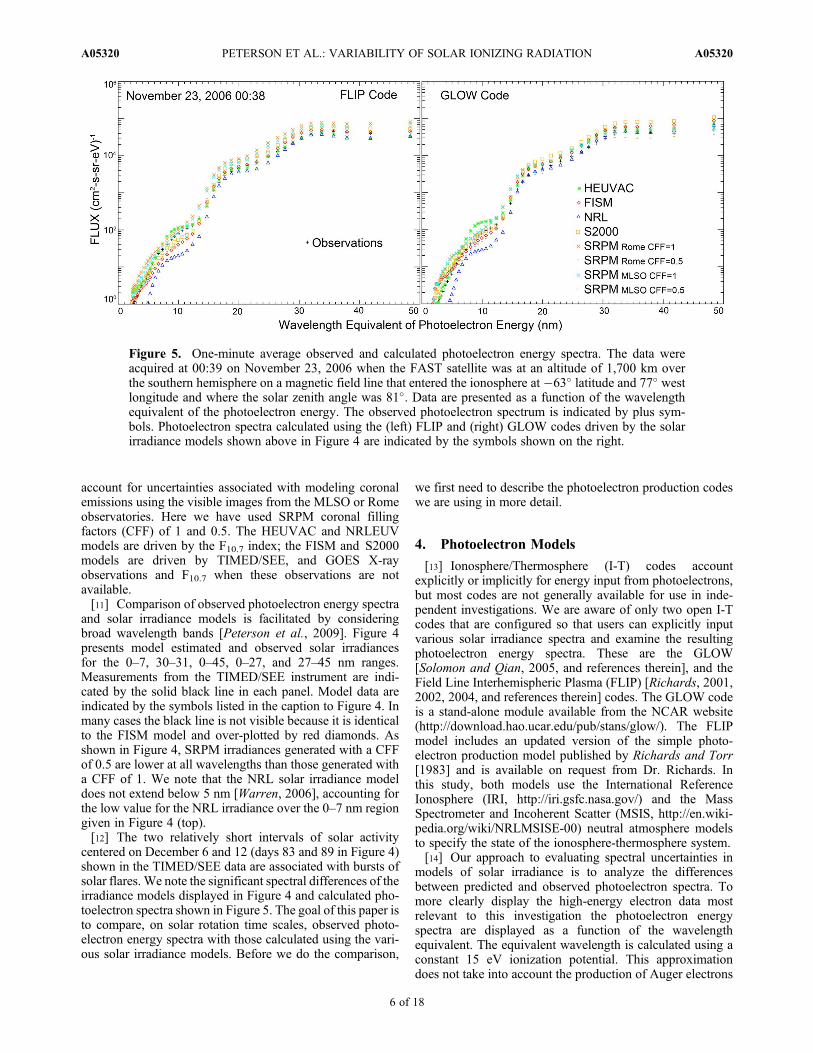
Figure 5. One-minute average observed and calculated photoelectron energy spectra. The data wereacquired at 00:39 on November 23, 2006 when the FAST satellite was at an altitude of 1,700 km overthe southern hemisphere on a magnetic field line that entered the ionosphere at �63� latitude and 77� westlongitude and where the solar zenith angle was 81�. Data are presented as a function of the wavelengthequivalent of the photoelectron energy. The observed photoelectron spectrum is indicated by plus sym-bols. Photoelectron spectra calculated using the (left) FLIP and (right) GLOW codes driven by the solarirradiance models shown above in Figure 4 are indicated by the symbols shown on the right.


6 of 18

from atomic oxygen or molecular nitrogen which haveenergies above 250 eV [Richards et al., 2006; Petersonet al., 2009]. Photoelectron energy spectra as a function ofequivalent wavelength from the code and solar irradiancemodel pairs used in this investigation are shown in Figure 5for the one-minute period identified in the caption. Thepredicted and observed photoelectron spectra agree withinan order of magnitude for this interval.[15] Another measure of differences between observed and

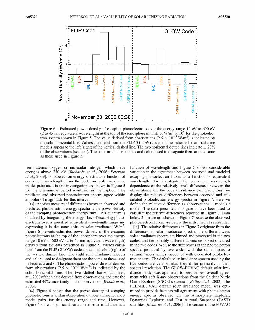
predicted photoelectron energy spectra is the power densityof the escaping photoelectron energy flux. This quantity isobtained by integrating the energy flux of escaping photo-electrons over a specified equivalent wavelength range andexpressing it in the same units as solar irradiance, W/m2.Figure 6 presents estimated power density of the escapingphotoelectrons at the top of the ionosphere over the energyrange 10 eV to 600 eV (2 to 45 nm equivalent wavelength)derived from the data presented in Figure 5. Values calcu-lated from the FLIP (GLOW) code appear in the left (right) ofthe vertical dashed line. The eight solar irradiance modelsand colors used to designate them are the same as those usedin Figures 5 and 6. The photoelectron power density derivedfrom observations (2.5 � 10�5 W/m2) is indicated by thesolid horizontal line. The two dotted horizontal lines,at�20% of the value derived from observations, indicate theestimated 40% uncertainty in the observations [Woods et al.,2003].[16] Figure 6 shows that the power density of escaping

photoelectrons is within observational uncertainties for mostmodel pairs for this energy range and time. However,Figure 4 shows significant variation in solar irradiance as a

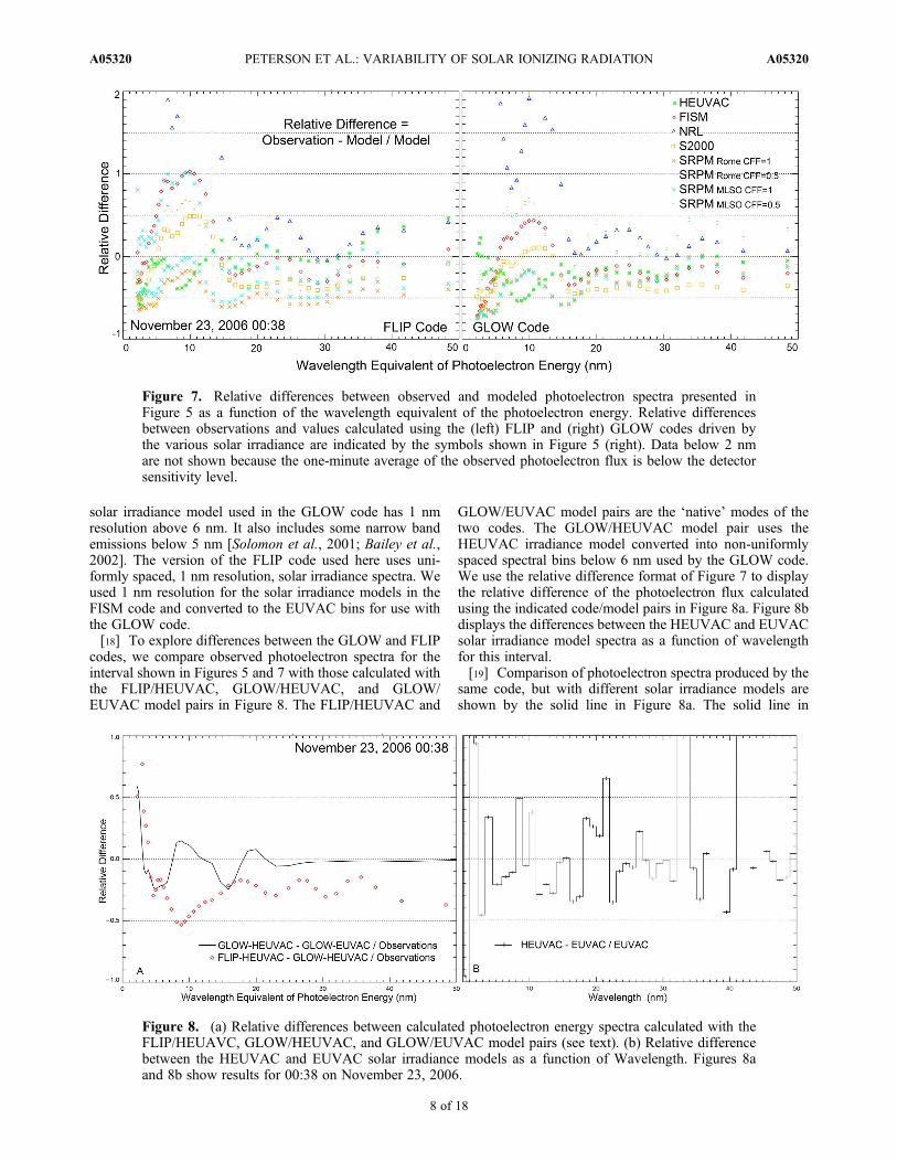
function of wavelength and Figure 5 shows considerablevariation in the agreement between observed and modeledescaping photoelectron fluxes as a function of equivalentwavelength. To investigate the equivalent wavelengthdependence of the relatively small differences between theobservations and the code / irradiance pair predictions, wedisplay the relative differences between observed and cal-culated photoelectron energy spectra in Figure 7. Here wedefine the relative difference as (observations – model) /model. The data presented in Figure 5 have been used tocalculate the relative differences reported in Figure 7. Databelow 2 nm are not shown in Figure 7 because the observedphotoelectron fluxes are below the instrumental sensitivity.[17] The relative differences in Figure 7 originate from the

differences in solar irradiance spectra, the different wayssolar irradiance spectra are binned and processed in the twocodes, and the possibly different atomic cross sections usedin the two codes. We use the differences in the photoelectronspectra produced by two codes with the same inputs toestimate uncertainties associated with calculated photoelec-tron spectra. The default solar irradiance spectra used by thetwo codes are very similar; they differ primarily in theirspectral resolution. The GLOW-EUVAC default solar irra-diance model was optimized to provide best overall agree-ment with soft X-ray observations from the Student NitricOxide Explorer (SNOE) spacecraft [Bailey et al., 2002]. TheFLIP-HEUVAC default solar irradiance model was opti-mized to provide best overall agreement with photoelectronenergy spectra observed on the Atmosphere Explorer,Dynamics Explorer, and Fast Auroral Snapshot (FAST)satellites [Richards et al., 2006]. The version of the EUVAC

Figure 6. Estimated power density of escaping photoelectrons over the energy range 10 eV to 600 eV(2 to 45 nm equivalent wavelength) at the top of the ionosphere in units of W/m2 � 105 for the photoelec-tron spectra shown in Figure 5. The value derived from observations (2.5 � 10�5 W/m2) is indicated bythe solid horizontal line. Values calculated from the FLIP (GLOW) code and the indicated solar irradiancemodels appear to the left (right) of the vertical dashed line. The two horizontal dotted lines indicate � 20%of the observations (see text). The solar irradiance models and colors used to designate them are the sameas those used in Figure 5.


7 of 18

solar irradiance model used in the GLOW code has 1 nmresolution above 6 nm. It also includes some narrow bandemissions below 5 nm [Solomon et al., 2001; Bailey et al.,2002]. The version of the FLIP code used here uses uni-formly spaced, 1 nm resolution, solar irradiance spectra. Weused 1 nm resolution for the solar irradiance models in theFISM code and converted to the EUVAC bins for use withthe GLOW code.[18] To explore differences between the GLOW and FLIP

codes, we compare observed photoelectron spectra for theinterval shown in Figures 5 and 7 with those calculated withthe FLIP/HEUVAC, GLOW/HEUVAC, and GLOW/EUVAC model pairs in Figure 8. The FLIP/HEUVAC and

GLOW/EUVAC model pairs are the ‘native’ modes of thetwo codes. The GLOW/HEUVAC model pair uses theHEUVAC irradiance model converted into non-uniformlyspaced spectral bins below 6 nm used by the GLOW code.We use the relative difference format of Figure 7 to displaythe relative difference of the photoelectron flux calculatedusing the indicated code/model pairs in Figure 8a. Figure 8bdisplays the differences between the HEUVAC and EUVACsolar irradiance model spectra as a function of wavelengthfor this interval.[19] Comparison of photoelectron spectra produced by the

same code, but with different solar irradiance models areshown by the solid line in Figure 8a. The solid line in

Figure 7. Relative differences between observed and modeled photoelectron spectra presented inFigure 5 as a function of the wavelength equivalent of the photoelectron energy. Relative differencesbetween observations and values calculated using the (left) FLIP and (right) GLOW codes driven bythe various solar irradiance are indicated by the symbols shown in Figure 5 (right). Data below 2 nmare not shown because the one-minute average of the observed photoelectron flux is below the detectorsensitivity level.

Figure 8. (a) Relative differences between calculated photoelectron energy spectra calculated with theFLIP/HEUAVC, GLOW/HEUVAC, and GLOW/EUVAC model pairs (see text). (b) Relative differencebetween the HEUVAC and EUVAC solar irradiance models as a function of Wavelength. Figures 8aand 8b show results for 00:38 on November 23, 2006.


8 of 18

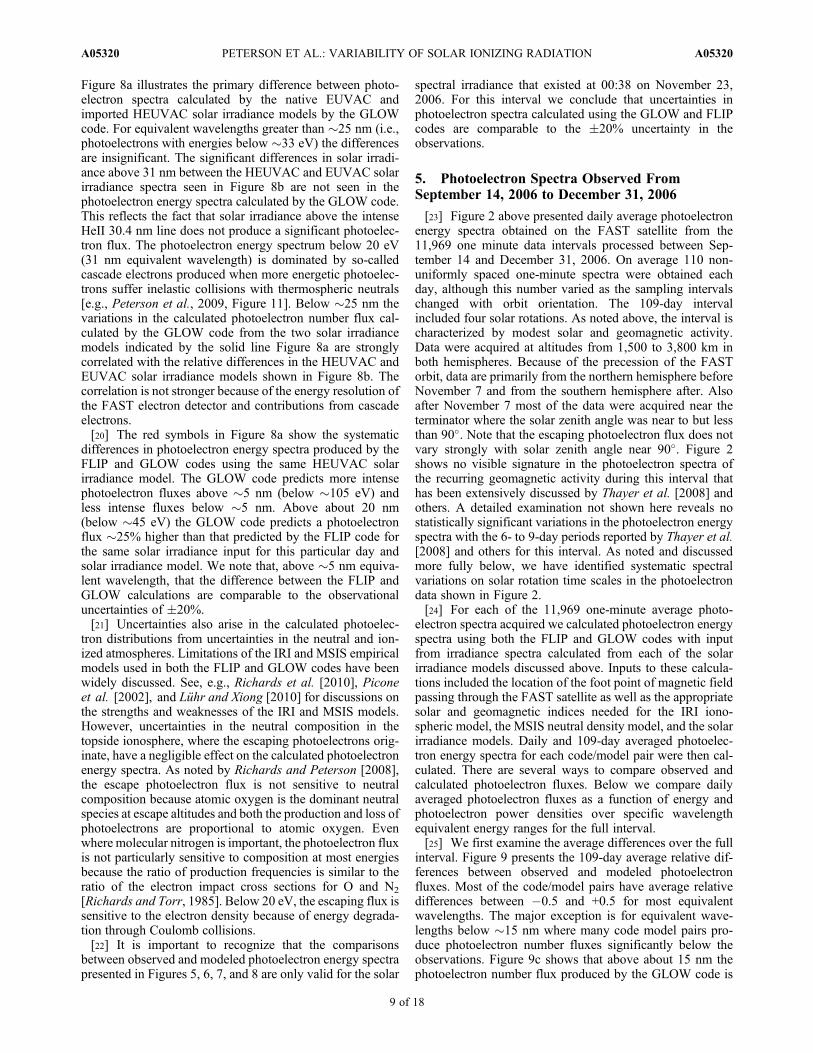
Figure 8a illustrates the primary difference between photo-electron spectra calculated by the native EUVAC andimported HEUVAC solar irradiance models by the GLOWcode. For equivalent wavelengths greater than �25 nm (i.e.,photoelectrons with energies below �33 eV) the differencesare insignificant. The significant differences in solar irradi-ance above 31 nm between the HEUVAC and EUVAC solarirradiance spectra seen in Figure 8b are not seen in thephotoelectron energy spectra calculated by the GLOW code.This reflects the fact that solar irradiance above the intenseHeII 30.4 nm line does not produce a significant photoelec-tron flux. The photoelectron energy spectrum below 20 eV(31 nm equivalent wavelength) is dominated by so-calledcascade electrons produced when more energetic photoelec-trons suffer inelastic collisions with thermospheric neutrals[e.g., Peterson et al., 2009, Figure 11]. Below �25 nm thevariations in the calculated photoelectron number flux cal-culated by the GLOW code from the two solar irradiancemodels indicated by the solid line Figure 8a are stronglycorrelated with the relative differences in the HEUVAC andEUVAC solar irradiance models shown in Figure 8b. Thecorrelation is not stronger because of the energy resolution ofthe FAST electron detector and contributions from cascadeelectrons.[20] The red symbols in Figure 8a show the systematic

differences in photoelectron energy spectra produced by theFLIP and GLOW codes using the same HEUVAC solarirradiance model. The GLOW code predicts more intensephotoelectron fluxes above �5 nm (below �105 eV) andless intense fluxes below �5 nm. Above about 20 nm(below �45 eV) the GLOW code predicts a photoelectronflux �25% higher than that predicted by the FLIP code forthe same solar irradiance input for this particular day andsolar irradiance model. We note that, above �5 nm equiva-lent wavelength, that the difference between the FLIP andGLOW calculations are comparable to the observationaluncertainties of �20%.[21] Uncertainties also arise in the calculated photoelec-

tron distributions from uncertainties in the neutral and ion-ized atmospheres. Limitations of the IRI and MSIS empiricalmodels used in both the FLIP and GLOW codes have beenwidely discussed. See, e.g., Richards et al. [2010], Piconeet al. [2002], and Lühr and Xiong [2010] for discussions onthe strengths and weaknesses of the IRI and MSIS models.However, uncertainties in the neutral composition in thetopside ionosphere, where the escaping photoelectrons orig-inate, have a negligible effect on the calculated photoelectronenergy spectra. As noted by Richards and Peterson [2008],the escape photoelectron flux is not sensitive to neutralcomposition because atomic oxygen is the dominant neutralspecies at escape altitudes and both the production and loss ofphotoelectrons are proportional to atomic oxygen. Evenwhere molecular nitrogen is important, the photoelectron fluxis not particularly sensitive to composition at most energiesbecause the ratio of production frequencies is similar to theratio of the electron impact cross sections for O and N2

[Richards and Torr, 1985]. Below 20 eV, the escaping flux issensitive to the electron density because of energy degrada-tion through Coulomb collisions.[22] It is important to recognize that the comparisons

between observed and modeled photoelectron energy spectrapresented in Figures 5, 6, 7, and 8 are only valid for the solar

spectral irradiance that existed at 00:38 on November 23,2006. For this interval we conclude that uncertainties inphotoelectron spectra calculated using the GLOW and FLIPcodes are comparable to the �20% uncertainty in theobservations.

5. Photoelectron Spectra Observed FromSeptember 14, 2006 to December 31, 2006

[23] Figure 2 above presented daily average photoelectronenergy spectra obtained on the FAST satellite from the11,969 one minute data intervals processed between Sep-tember 14 and December 31, 2006. On average 110 non-uniformly spaced one-minute spectra were obtained eachday, although this number varied as the sampling intervalschanged with orbit orientation. The 109-day intervalincluded four solar rotations. As noted above, the interval ischaracterized by modest solar and geomagnetic activity.Data were acquired at altitudes from 1,500 to 3,800 km inboth hemispheres. Because of the precession of the FASTorbit, data are primarily from the northern hemisphere beforeNovember 7 and from the southern hemisphere after. Alsoafter November 7 most of the data were acquired near theterminator where the solar zenith angle was near to but lessthan 90�. Note that the escaping photoelectron flux does notvary strongly with solar zenith angle near 90�. Figure 2shows no visible signature in the photoelectron spectra ofthe recurring geomagnetic activity during this interval thathas been extensively discussed by Thayer et al. [2008] andothers. A detailed examination not shown here reveals nostatistically significant variations in the photoelectron energyspectra with the 6- to 9-day periods reported by Thayer et al.[2008] and others for this interval. As noted and discussedmore fully below, we have identified systematic spectralvariations on solar rotation time scales in the photoelectrondata shown in Figure 2.[24] For each of the 11,969 one-minute average photo-

electron spectra acquired we calculated photoelectron energyspectra using both the FLIP and GLOW codes with inputfrom irradiance spectra calculated from each of the solarirradiance models discussed above. Inputs to these calcula-tions included the location of the foot point of magnetic fieldpassing through the FAST satellite as well as the appropriatesolar and geomagnetic indices needed for the IRI iono-spheric model, the MSIS neutral density model, and the solarirradiance models. Daily and 109-day averaged photoelec-tron energy spectra for each code/model pair were then cal-culated. There are several ways to compare observed andcalculated photoelectron fluxes. Below we compare dailyaveraged photoelectron fluxes as a function of energy andphotoelectron power densities over specific wavelengthequivalent energy ranges for the full interval.[25] We first examine the average differences over the full

interval. Figure 9 presents the 109-day average relative dif-ferences between observed and modeled photoelectronfluxes. Most of the code/model pairs have average relativedifferences between �0.5 and +0.5 for most equivalentwavelengths. The major exception is for equivalent wave-lengths below �15 nm where many code model pairs pro-duce photoelectron number fluxes significantly below theobservations. Figure 9c shows that above about 15 nm thephotoelectron number flux produced by the GLOW code is


9 of 18

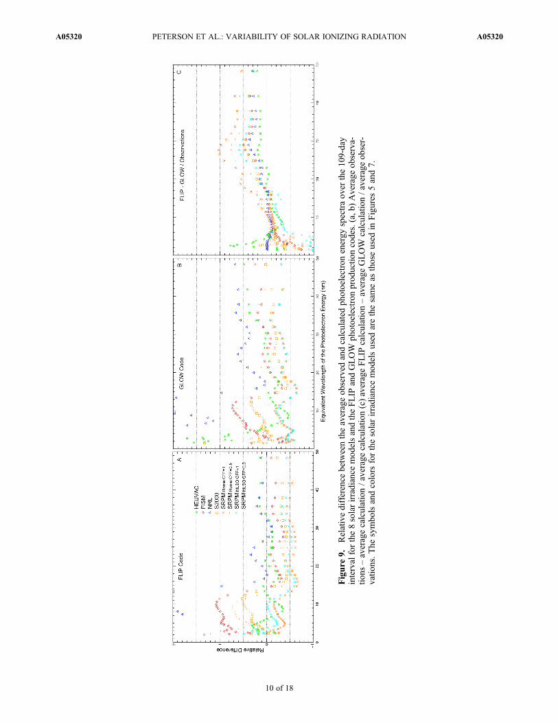
Figure

9.Relativedifference

betweentheaverageobserved

andcalculated

photoelectronenergy

spectraover

the109-day

intervalforthe8solarirradiance

modelsandtheFLIP

andGLOW

photoelectronproductio

ncodes.(a,b

)Average

observa-

tions

–averagecalculation/average

calculation(c)averageFLIP

calculation–averageGLOW

calculation/average

obser-

vatio

ns.The

symbolsandcolors

forthesolarirradiance

modelsused

arethesameas

thoseused

inFigures

5and7.


10 of 18

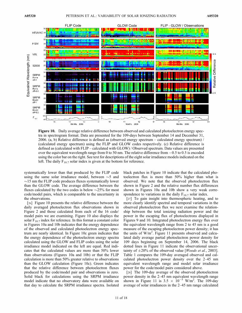
systematically lower than that produced by the FLIP codeusing the same solar irradiance model, between �5 and�15 nm the FLIP code produces fluxes systematically lowerthan the GLOW code. The average difference between thefluxes calculated by the two codes is below �25% for mostcode/model pairs, which is comparable to the uncertainty inthe observations.[26] Figure 10 presents the relative difference between the

daily averaged photoelectron flux observations shown inFigure 2 and those calculated from each of the 16 code/model pairs we are examining. Figure 10 also displays thesolar F10.7 index for reference. In this format a constant colorin Figures 10a and 10b indicates that the energy dependenceof the observed and calculated photoelectron energy spec-trum are nearly identical. In Figure 10c green indicates thatthe energy dependence of the photoelectron energy spectracalculated using the GLOW and FLIP codes using the solarirradiance model indicated on the left are equal. Red indi-cates that the calculated values are more than 50% lowerthan observations (Figures 10a and 10b) or that the FLIPcalculation is more than 50% greater relative to observationsthan the GLOW calculation (Figure 10c). Green indicatesthat the relative difference between photoelectron fluxesproduced by the code/model pair and observations is zero.Solid black for calculations using the SRPM irradiancemodel indicate that no observatory data were available onthat day to calculate the SRPM irradiance spectra. Isolated

black patches in Figure 10 indicate that the calculated pho-toelectron flux is more than 50% higher than what isobserved. We note that the observed photoelectron fluxshown in Figure 2 and the relative number flux differencesshown in Figures 10a and 10b show a very weak corre-spondence to variations in the daily F10.7 solar index.[27] To gain insight into thermospheric heating, and to

more clearly identify spectral and temporal variations in theobserved photoelectron flux we next examine the relation-ship between the total ionizing radiation power and thepower in the escaping flux of photoelectrons displayed inFigures 9 and 10. Integrated photoelectron energy flux overthe equivalent wavelength range from 2 to 45 nm is a goodmeasure of the escaping photoelectron power density; it hasthe units of W/m2. Figure 11 presents observed and calcu-lated daily average partial photoelectron power density for109 days beginning on September 14, 2006. The blackdotted lines in Figure 11 indicate the observational uncer-tainty of �20% of the observed value [Woods et al., 2003].Table 1 compares the 109-day averaged observed and cal-culated photoelectron power density over the 2–45 nmequivalent wavelength range and model solar irradiancepower for the code/model pairs considered above.[28] The 109-day average of the observed photoelectron

power density in the 2–45 nm equivalent wavelength rangeshown in Figure 11 is 3.5 � 10�5 W/m2. The 109-dayaverage of solar irradiances in the 2–45 nm range calculated

Figure 10. Daily average relative difference between observed and calculated photoelectron energy spec-tra in spectrogram format. Data are presented for the 109-days between September 14 and December 31,2006. (a, b) Relative difference is defined as (observed energy spectrum – calculated energy spectrum) /(calculated energy spectrum) using the FLIP and GLOW codes respectively. (c) Relative difference isdefined as (calculated with FLIP – calculated with GLOW) / Observed spectrum. Data values are presentedover the equivalent wavelength range from 0 to 50 nm. The relative difference from�0.5 to 0.5 is encodedusing the color bar on the right. See text for descriptions of the eight solar irradiance models indicated on theleft. The daily F10.7 solar index is given at the bottom for reference.


11 of 18

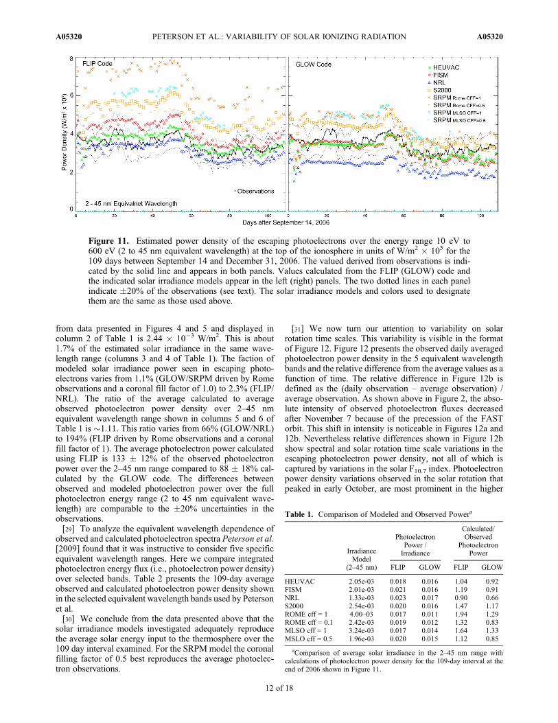
from data presented in Figures 4 and 5 and displayed incolumn 2 of Table 1 is 2.44 � 10�3 W/m2. This is about1.7% of the estimated solar irradiance in the same wave-length range (columns 3 and 4 of Table 1). The faction ofmodeled solar irradiance power seen in escaping photo-electrons varies from 1.1% (GLOW/SRPM driven by Romeobservations and a coronal fill factor of 1.0) to 2.3% (FLIP/NRL). The ratio of the average calculated to averageobserved photoelectron power density over 2–45 nmequivalent wavelength range shown in columns 5 and 6 ofTable 1 is �1.11. This ratio varies from 66% (GLOW/NRL)to 194% (FLIP driven by Rome observations and a coronalfill factor of 1). The average photoelectron power calculatedusing FLIP is 133 � 12% of the observed photoelectronpower over the 2–45 nm range compared to 88 � 18% cal-culated by the GLOW code. The differences betweenobserved and modeled photoelectron power over the fullphotoelectron energy range (2 to 45 nm equivalent wave-length) are comparable to the �20% uncertainties in theobservations.[29] To analyze the equivalent wavelength dependence of

observed and calculated photoelectron spectra Peterson et al.[2009] found that it was instructive to consider five specificequivalent wavelength ranges. Here we compare integratedphotoelectron energy flux (i.e., photoelectron power density)over selected bands. Table 2 presents the 109-day averageobserved and calculated photoelectron power density shownin the selected equivalent wavelength bands used by Petersonet al.[30] We conclude from the data presented above that the

solar irradiance models investigated adequately reproducethe average solar energy input to the thermosphere over the109 day interval examined. For the SRPM model the coronalfilling factor of 0.5 best reproduces the average photoelec-tron observations.

[31] We now turn our attention to variability on solarrotation time scales. This variability is visible in the formatof Figure 12. Figure 12 presents the observed daily averagedphotoelectron power density in the 5 equivalent wavelengthbands and the relative difference from the average values as afunction of time. The relative difference in Figure 12b isdefined as the (daily observation – average observation) /average observation. As shown above in Figure 2, the abso-lute intensity of observed photoelectron fluxes decreasedafter November 7 because of the precession of the FASTorbit. This shift in intensity is noticeable in Figures 12a and12b. Nevertheless relative differences shown in Figure 12bshow spectral and solar rotation time scale variations in theescaping photoelectron power density, not all of which iscaptured by variations in the solar F10.7 index. Photoelectronpower density variations observed in the solar rotation thatpeaked in early October, are most prominent in the higher

Figure 11. Estimated power density of the escaping photoelectrons over the energy range 10 eV to600 eV (2 to 45 nm equivalent wavelength) at the top of the ionosphere in units of W/m2 � 105 for the109 days between September 14 and December 31, 2006. The valued derived from observations is indi-cated by the solid line and appears in both panels. Values calculated from the FLIP (GLOW) code andthe indicated solar irradiance models appear in the left (right) panels. The two dotted lines in each panelindicate �20% of the observations (see text). The solar irradiance models and colors used to designatethem are the same as those used above.

Table 1. Comparison of Modeled and Observed Powera

IrradianceModel

(2–45 nm)

PhotoelectronPower /Irradiance

Calculated/Observed

PhotoelectronPower

FLIP GLOW FLIP GLOW

HEUVAC 2.05e-03 0.018 0.016 1.04 0.92FISM 2.01e-03 0.021 0.016 1.19 0.91NRL 1.33e-03 0.023 0.017 0.90 0.66S2000 2.54e-03 0.020 0.016 1.47 1.17ROME cff = 1 4.00–03 0.017 0.011 1.94 1.29ROME cff = 0.1 2.42e-03 0.019 0.012 1.32 0.83MLSO cff = 1 3.24e-03 0.017 0.014 1.64 1.33MSLO cff = 0.5 1.96e-03 0.020 0.015 1.12 0.85

aComparison of average solar irradiance in the 2–45 nm range withcalculations of photoelectron power density for the 109-day interval at theend of 2006 shown in Figure 11.


12 of 18

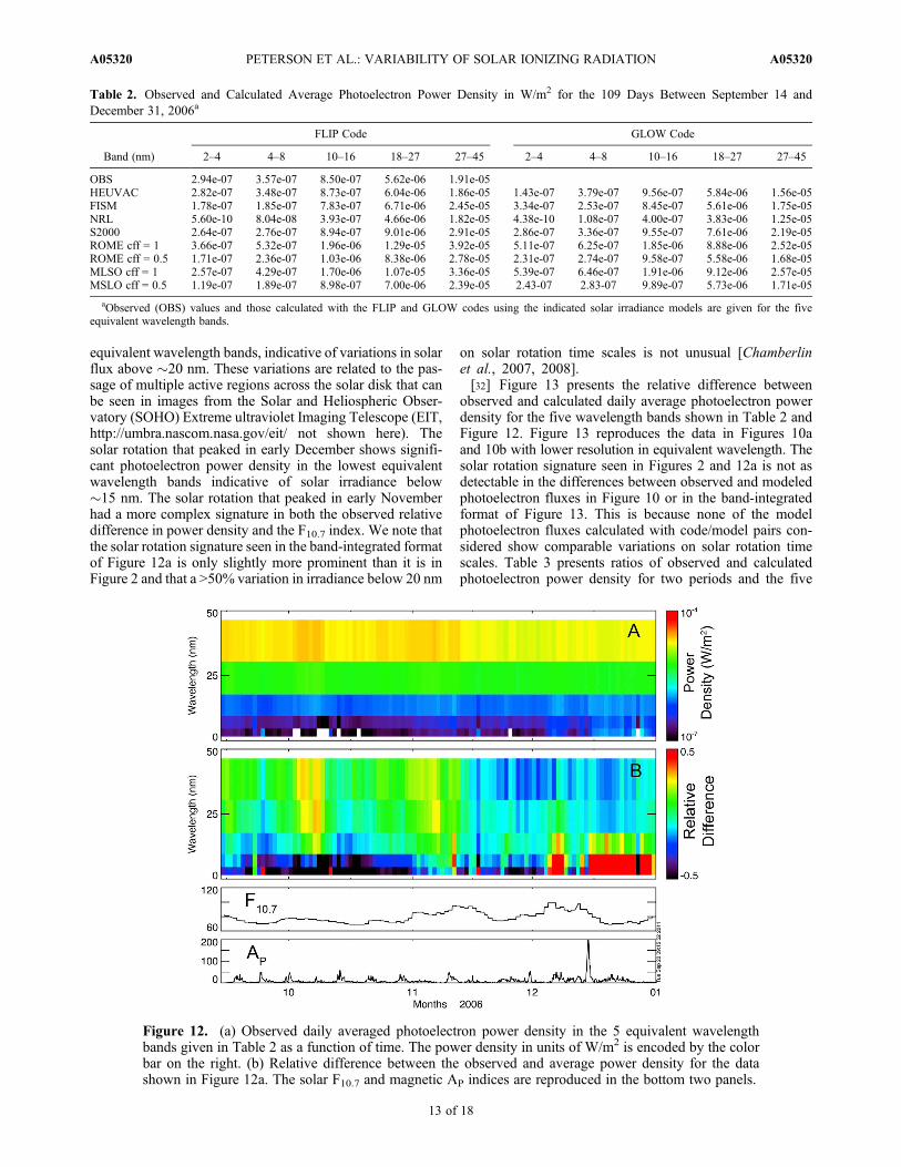
equivalent wavelength bands, indicative of variations in solarflux above �20 nm. These variations are related to the pas-sage of multiple active regions across the solar disk that canbe seen in images from the Solar and Heliospheric Obser-vatory (SOHO) Extreme ultraviolet Imaging Telescope (EIT,http://umbra.nascom.nasa.gov/eit/ not shown here). Thesolar rotation that peaked in early December shows signifi-cant photoelectron power density in the lowest equivalentwavelength bands indicative of solar irradiance below�15 nm. The solar rotation that peaked in early Novemberhad a more complex signature in both the observed relativedifference in power density and the F10.7 index. We note thatthe solar rotation signature seen in the band-integrated formatof Figure 12a is only slightly more prominent than it is inFigure 2 and that a >50% variation in irradiance below 20 nm

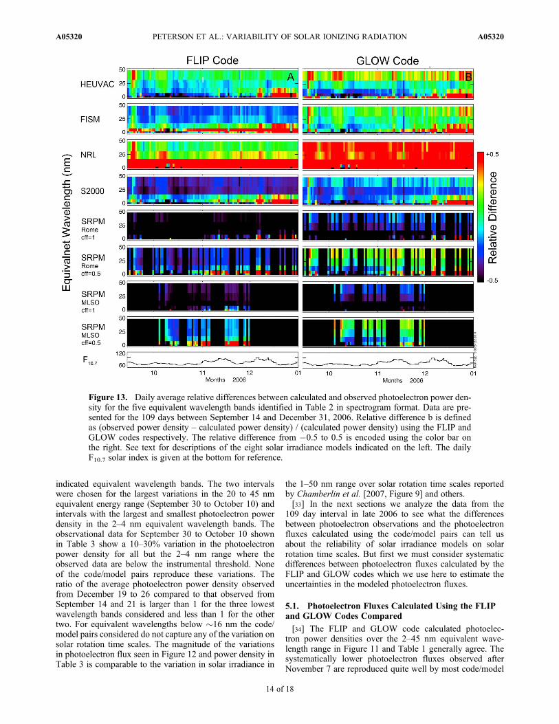
on solar rotation time scales is not unusual [Chamberlinet al., 2007, 2008].[32] Figure 13 presents the relative difference between

observed and calculated daily average photoelectron powerdensity for the five wavelength bands shown in Table 2 andFigure 12. Figure 13 reproduces the data in Figures 10aand 10b with lower resolution in equivalent wavelength. Thesolar rotation signature seen in Figures 2 and 12a is not asdetectable in the differences between observed and modeledphotoelectron fluxes in Figure 10 or in the band-integratedformat of Figure 13. This is because none of the modelphotoelectron fluxes calculated with code/model pairs con-sidered show comparable variations on solar rotation timescales. Table 3 presents ratios of observed and calculatedphotoelectron power density for two periods and the five

Figure 12. (a) Observed daily averaged photoelectron power density in the 5 equivalent wavelengthbands given in Table 2 as a function of time. The power density in units of W/m2 is encoded by the colorbar on the right. (b) Relative difference between the observed and average power density for the datashown in Figure 12a. The solar F10.7 and magnetic AP indices are reproduced in the bottom two panels.

Table 2. Observed and Calculated Average Photoelectron Power Density in W/m2 for the 109 Days Between September 14 andDecember 31, 2006a

Band (nm)

FLIP Code GLOW Code

2–4 4–8 10–16 18–27 27–45 2–4 4–8 10–16 18–27 27–45

OBS 2.94e-07 3.57e-07 8.50e-07 5.62e-06 1.91e-05HEUVAC 2.82e-07 3.48e-07 8.73e-07 6.04e-06 1.86e-05 1.43e-07 3.79e-07 9.56e-07 5.84e-06 1.56e-05FISM 1.78e-07 1.85e-07 7.83e-07 6.71e-06 2.45e-05 3.34e-07 2.53e-07 8.45e-07 5.61e-06 1.75e-05NRL 5.60e-10 8.04e-08 3.93e-07 4.66e-06 1.82e-05 4.38e-10 1.08e-07 4.00e-07 3.83e-06 1.25e-05S2000 2.64e-07 2.76e-07 8.94e-07 9.01e-06 2.91e-05 2.86e-07 3.36e-07 9.55e-07 7.61e-06 2.19e-05ROME cff = 1 3.66e-07 5.32e-07 1.96e-06 1.29e-05 3.92e-05 5.11e-07 6.25e-07 1.85e-06 8.88e-06 2.52e-05ROME cff = 0.5 1.71e-07 2.36e-07 1.03e-06 8.38e-06 2.78e-05 2.31e-07 2.74e-07 9.58e-07 5.58e-06 1.68e-05MLSO cff = 1 2.57e-07 4.29e-07 1.70e-06 1.07e-05 3.36e-05 5.39e-07 6.46e-07 1.91e-06 9.12e-06 2.57e-05MSLO cff = 0.5 1.19e-07 1.89e-07 8.98e-07 7.00e-06 2.39e-05 2.43-07 2.83-07 9.89e-07 5.73e-06 1.71e-05

aObserved (OBS) values and those calculated with the FLIP and GLOW codes using the indicated solar irradiance models are given for the fiveequivalent wavelength bands.


13 of 18

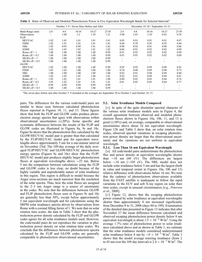
indicated equivalent wavelength bands. The two intervalswere chosen for the largest variations in the 20 to 45 nmequivalent energy range (September 30 to October 10) andintervals with the largest and smallest photoelectron powerdensity in the 2–4 nm equivalent wavelength bands. Theobservational data for September 30 to October 10 shownin Table 3 show a 10–30% variation in the photoelectronpower density for all but the 2–4 nm range where theobserved data are below the instrumental threshold. Noneof the code/model pairs reproduce these variations. Theratio of the average photoelectron power density observedfrom December 19 to 26 compared to that observed fromSeptember 14 and 21 is larger than 1 for the three lowestwavelength bands considered and less than 1 for the othertwo. For equivalent wavelengths below �16 nm the code/model pairs considered do not capture any of the variation onsolar rotation time scales. The magnitude of the variationsin photoelectron flux seen in Figure 12 and power density inTable 3 is comparable to the variation in solar irradiance in

the 1–50 nm range over solar rotation time scales reportedby Chamberlin et al. [2007, Figure 9] and others.[33] In the next sections we analyze the data from the

109 day interval in late 2006 to see what the differencesbetween photoelectron observations and the photoelectronfluxes calculated using the code/model pairs can tell usabout the reliability of solar irradiance models on solarrotation time scales. But first we must consider systematicdifferences between photoelectron fluxes calculated by theFLIP and GLOW codes which we use here to estimate theuncertainties in the modeled photoelectron fluxes.

5.1. Photoelectron Fluxes Calculated Using the FLIPand GLOW Codes Compared

[34] The FLIP and GLOW code calculated photoelec-tron power densities over the 2–45 nm equivalent wave-length range in Figure 11 and Table 1 generally agree. Thesystematically lower photoelectron fluxes observed afterNovember 7 are reproduced quite well by most code/model

Figure 13. Daily average relative differences between calculated and observed photoelectron power den-sity for the five equivalent wavelength bands identified in Table 2 in spectrogram format. Data are pre-sented for the 109 days between September 14 and December 31, 2006. Relative difference b is definedas (observed power density – calculated power density) / (calculated power density) using the FLIP andGLOW codes respectively. The relative difference from �0.5 to 0.5 is encoded using the color bar onthe right. See text for descriptions of the eight solar irradiance models indicated on the left. The dailyF10.7 solar index is given at the bottom for reference.


14 of 18

pairs. The differences for the various code/model pairs aresimilar to those seen between calculated photoelectronfluxes reported in Figures 10, 11, and 13. These figuresshow that both the FLIP and GLOW codes produce photo-electron energy spectra that agree with observations withinobservational uncertainties (�20%). Some specific andsystematic differences between the results of the FLIP andGLOW codes are illustrated in Figures 8a, 9c and 10c.Figure 8a shows that the photoelectron flux calculated by theGLOW/HEUVAC model pair is greater than that calculatedby the FLIP/HEUVAC model pair for equivalent wave-lengths above approximately 5 nm for a one-minute intervalon November 23rd. The 109-day average of the daily aver-aged FLIP/HEUVAC and GLOW/HEUVAC photoelectronenergy spectra (Figures 9c and 10c) show that the FLIP/HEUVAC model pair produces slightly larger photoelectronfluxes at equivalent wavelengths above �25 nm. Below5 nm the comparison between calculations using the FLIPand GLOW codes is less clear, no doubt because of thehighly variable and unpredictable nature of solar irradiancein this region. This region is difficult to model because theAuger cross-sections are much narrower than the resolutionof the solar spectra. Thus, how the solar fluxes are assignedto the 2–3 nm Auger range is a source of uncertaintyin the codes. We note that the differences between GLOWand FLIP photoelectron fluxes seen in Figures 9c and 10care generally less than 50%, except below approximately5 nm equivalent wavelength and for calculations using theSRPM solar irradiance spectra driven by observations fromRome with a coronal filling factor of 1. We note that on solarrotation time scales, the data in Table 3 show that the pho-toelectron power density calculated by the FLIP and GLOWcodes agrees for all solar irradiance models used. However,the code/model pairs do not reproduce the variation in pho-toelectron power density on solar rotation time scales. Weconclude that the differences between photoelectron spectracalculated by the FLIP and GLOW codes are generallycomparable to photoelectron observational uncertainties.

5.2. Solar Irradiance Models Compared

[35] In spite of the quite dissimilar spectral character ofthe various solar irradiance models seen in Figure 4, theoverall agreement between observed and modeled photo-electron fluxes shown in Figures 10a, 10b, 11, and 13 isgood (�50%) and, on average, comparable to observationaluncertainties above about 16 nm equivalent wavelength.Figure 12b and Table 3 show that, on solar rotation timescales, observed spectral variations in escaping photoelec-tron power density are larger than the observational uncer-tainty and the variations are not uniform in equivalentwavelength.5.2.1. Less Than 16 nm Equivalent Wavelength[36] All code/model pairs underestimate the photoelectron

flux and power density at equivalent wavelengths shorterthan �16 nm (60 eV). The differences are largestbelow �10 nm (�105 eV). The NRL model does notinclude solar irradiance below 5 nm and has the largest (bothin value and temporal extent in Figures 10a, 10b and 13)relative difference with observations below 16 nm. We notethat the cadence of photoelectron observations availablefrom the FAST satellite is inadequate to follow the rapidvariations in the EUV and soft X-ray region on solar flaretime scales, except in unusual circumstances [e.g., Petersonet al., 2008].[37] Figure 12, shows that the escaping photoelectron

power created by solar irradiance at equivalent wavelengthsshorter than approximately 8 nm increased significantlyfrom December 8 to 31, 2006 (days 84 to 109). Examinationof the detailed data presented in Figure 13 indicates that afterNovember 27 the mean difference between calculated andobserved escaping photoelectron power density below 8 nmequivalent wavelength is about 1.5 � 10�6 W/m2. Using theaverage 1.7% ratio of photoelectron power to solar irradi-ance calculated above and as shown in Table 1, we estimatethat the solar irradiance models considered underestimatedsolar irradiance below 8 nm by �9 � 10�5 W/m2. Table 1shows that the model average ionizing irradiance (from 2to 45 nm over the 109 day interval) is 2.4� 10�3 W/m2. The

Table 3. Ratio of Observed and Modeled Photoelectron Power in Five Equivalent Wavelength Bands for Selected Intervalsa

October 3–9 / Seven Days Before and After December 19–26 / September 14–21

Band Range (nm) 2:4 4:8 10:16 18:27 27:45 2:4 4:8 10:16 18:27 27:45Observations - 1.08 1.2 1.29 1.21 5.08 2.63 1.29 0.83 0.76FLIPHEUVAC 1.02 1.01 1.01 1.01 1.01 0.83 0.91 0.91 0.91 0.87FISM 1.02 1.01 1.01 1.01 1.01 0.68 0.79 0.93 0.93 0.84NRL 1.02 0.95 0.99 1.01 1.02 0.90 0.92 0.91 0.90 0.86S2000 1.02 1.03 1.02 1.01 1.02 0,86 0.91 0.92 0.92 0.89Rome cff = 1 1.00 1.00 1.00 1.00 0.99 0.91 0.93 0.92 0.92 0.89Rome cff = 0.5 1.00 1.00 1.00 1.00 0.99 0.91 0.93 0.92 0.92 0.88MLSO cff = 1 1.00 1.00 1.00 1.00 0.99 - - - - -MLSO cff = 0.5 1.00 1.00 1.00 1.00 0.99 - - - - -

GLOWHEUVAC 1.02 1.00 1.00 1.00 0.99 0.95 0.92 0.89 0.90 0.82FISM 1.03 1.02 1.00 1.00 1.00 0.70 0.80 0.89 0.90 0.75NRL 1.00 1.00 1.00 1.00 1.00 0.92 0.91 0.88 0.89 0.80S2000 1.02 1.03 1.01 1.00 1.01 0.92 0.91 0.89 0.89 0.81Rome cff = 1 1.03 1.02 1.01 1.01 1.00 0.80 0.85 0.85 0.84 0.76Rome cff = 0.5 1.03 1.02 1.01 1.01 1.01 0.81 0.85 0.85 0.84 0.77MLSO cff = 1 0.99 0.99 0.99 0.99 0.99 - - - - -MLSO cff = 0.5 1.00 1.00 1.00 1.00 0.99 - - - - -

aThe seven days before and after October 3–9 included in the averages are September 30 to October 2 and October 10–12.


15 of 18

irradiance below 8 nm represents only about 4% of theaverage model ionizing irradiance and photoelectron powerdensity for the 109 days, but for the interval after November27 it is about 10 times the average modeled solar irradianceand photoelectron power density.[38] Table 3 shows that during a solar rotation period

where there is little soft X-ray irradiance for wavelengthsbelow 16 nm all code/model pairs predict essentially novariation in photoelectron power density. The observedvariation in photoelectron power however is up to 20% inthe 10–16 nm equivalent wavelength band. Because thecontribution of cascade electrons is not dominant below31 nm the spectral variation in photoelectron power reflectsthe spectral variation in solar irradiance quite well.[39] The underestimated irradiance power below 16 nm in

the solar irradiance models inferred from photoelectronpower density observations discussed above has importantconsequences in large-scale thermospheric models. This isconsistent with earlier reports that solar irradiance in the softX-ray range is an important and highly variable thermo-spheric energy source [e.g., Richards et al., 1994; Baileyet al., 2002; Peterson et al., 2009]. As noted by Baileyet al. [2002] and many others, the soft X-ray ionizing radi-ation has a significant effect on nitric oxide chemistry andtherefore thermospheric dynamics. Large-scale models thatrely on the irradiance models considered here, including thedata driven FISM model, systematically underestimate thevariation of nitric oxide production over solar rotation timescales by sometimes by an order of magnitude.5.2.2. Equivalent Wavelength Above 16 nm[40] Two factors, cascade electrons and systematic differ-

ences between the FLIP and GLOW code calculations,complicate analysis above 16 nm. The nearly direct rela-tionship between ionizing radiation below 16 nm and theresulting observed escaping photoelectron power densitystarts to break down above about 16 nm. As noted above,cascade electrons dominate the photoelectron energy spec-trum above 31 nm equivalent wavelength. The systematicdifferences between photoelectron fluxes calculated usingthe FLIP and GLOW codes shown in Figures 9c and 10c arereflected in Table 1, which shows the photoelectron powerdensity in the 27–45 nm band calculated using the FLIPcode is greater than that calculated using the GLOW code. InFigure 13 and Tables 2 and 3, we considered two broadequivalent energy bands above 16 nm: 18–27 and 27–45 nm. Because of these complications we focus our anal-ysis on the 18–27 nm band.[41] On average, the code/model pairs considered repro-

duced the 109-day average photoelectron power density inthe 18–27 nm band quite well. The generally uniform colorsin Figure 13 for this band for all code/model pairs except theGLOW/NRL indicate good agreement between the observedand calculated photoelectron fluxes as a function time.Table 3 shows, however, that the observations and modelsdiffer on solar rotation time scales. For the solar rotationperiod from October 3–9, where there is little or no softX-ray irradiance, the code/model pairs calculated less than2% variation in the photoelectron power density in the 18–26 nm band compared to the 29% observed variation. Forthe intervals with significant soft X-ray variability (Decem-ber 19–26 compared to September 14–21), the agreementbetween observations and calculations is as expected from

observational uncertainties. Table 3 shows that for the 18–27 nm bin, the code/model pairs predict an 89 � 3% varia-tion compared to the 83% observed.5.2.3. Other Details Regarding the Agreement BetweenObserved and Calculated Escaping Photoelectrons[42] The data presented above show that our technique is

most sensitive to variations in solar irradiance at wave-lengths shorter than �31 nm (greater 24 eV equivalentenergy) where so-called cascade electrons do not dominatethe photoelectron energy spectrum. Table 2 shows that onlythe FLIP/HEUVAC model pair calculates the 109-dayaverage photoelectron power density within observationaluncertainties for all five equivalent wavelength bands con-sidered. Four GLOW/model pairs calculate power densitywithin the observational uncertainties for 4 of the 5 bands(HEUVAC, FISM, and the SRPM driven by both Rome andMLSO observations with a coronal filling factor of 0.5). Ingeneral the SRPM model with a coronal filling factor of0.5 best reproduces the observed photoelectron power den-sity reported in Figure 13 and Table 2.[43] The four poorest model pair calculations of 109-day

average photoelectron power density with calculated powerdensity values outside observational uncertainties for all 5energy bands are FLIP/SRPM, Rome, cff =1 and GLOW/NRL and SRPM with cff =1. Model pairs having powerdensity for 4 of 5 bands outside observational uncertaintiesinclude FLIP/SRPM, cff =0.5 and GLOW/SRPM, cff =1.[44] The decrease in escaping photoelectron power density

associated with local minima of the F10.7 index near Sep-tember 27 and October 1 (days 14 and 35) is not wellreproduced by any code/model pair for all of the equivalentwavelength ranges shown in Figure 13. The disagreement isgenerally greater than observational uncertainties. Thisconfirms, yet again, that the F10.7 index does not capture allsolar XUV and EUV irradiance variability [see, e.g., Dudokde Wit et al., 2009; Maruyama, 2011].

6. Summary and Conclusions

[45] We analyzed 11,969 one-minute average photoelec-tron energy spectra obtained during the 109 days fromSeptember 14 and December 31, 2006. During this intervalgeomagnetic activity was modest. The AP index ranged from0 to 236 with modest intensifications up to approximately 50at regular intervals. Solar activity was moderate with theF10.7 index ranging from 69 to 99. Four X class solar flareswere observed in December. We presented the solar irradi-ance observations available for this interval. We consideredfive widely used solar irradiance models (e.g., HEUVAC,FISM, NRL, S2000, and SRPM) to fill spectral and temporalgaps in the observations. We compared observed and mod-eled solar irradiances in Figure 4 using the FLIP and GLOWphotoelectron production codes with each of the solar irra-diance models. We showed that comparison of observed andcalculated escaping photoelectrons is most sensitive to var-iations in solar irradiance at wavelengths shorter than around31 nm (greater 24 eV equivalent energy) where so-calledcascade electrons do not dominate the photoelectron energyspectrum. We noted that uncertainties in the neutral compo-sition in the topside ionosphere, where the escaping photo-electrons originate, have a negligible effect on the calculatedphotoelectron energy spectra. On average we found that


16 of 18

about 1.7% of the solar ionizing radiation in the range 2–45 nm was observed in the escaping photoelectron flux.[46] Not unexpectedly, we found that the highly variable

solar irradiance below 8 nm is not fully captured in any ofthe irradiance models considered here. This is true both forsolar irradiance models driven by the F10.7 solar radio flux(HEUVAC and NRL) and those driven by other observationsand proxies (FISM, S2000, and SRPM). We estimated thatthe model solar irradiances were approximately 30% belowthose required to account for the increased photoelectronpower density at equivalent wavelengths below 10 nm(above 105 eV during the modest solar activity in December2006). During more active solar activity, Chamberlin et al.[2007] note that the Flare Irradiance Spectral Model (FISM)based on TIMED/SEE observations has uncertaintiesof �40%. The consequences are that large-scale models thatrely on the irradiance models considered here, including thedata driven FISM model, systematically underestimate thevariation of nitric oxide production over solar rotation timescales. The new solar irradiance measurements from thehigher temporal cadence and higher spectral resolutionExtreme Ultraviolet Variability Experiment (EVE) on theSolar Dynamics Observatory (SDO) [Woods et al., 2010]appear promising to resolve some of these differences in thephotoelectron comparisons for the shorter wavelengths;however, SDO EVE observations did not start until 2010 andthus do not overlap with these photoelectron measurements.[47] Considering the average photoelectron flux observed

in late 2006, our results indicate that even though the solarirradiance models we considered have significantly differentspectral charters, reasonable estimates of the heating effectsof photoelectrons are possible with both codes except duringperiods of activity changes during solar rotations. We foundthat none of the irradiance models was much better than theothers when used to calculate 109-day average escapingphotoelectron power density. However, the best agreementbetween 109-day average observations and irradiance mod-els was from the HEUVAC, FISM, and the SRPM with acoronal filling factor of 0.5. We note that these models aredriven by the F10.7 solar radio flux (HEUVAC) and othertypes of observations (FISM, EUV and XUV observations,and SRPM, solar visible images).[48] On solar rotation time scales we find that none of the

code/model pairs capture the variability of the observedphotoelectron power density (or flux) within the �20%observational uncertainties. During the solar rotation thatpeaked in early October 2006 all code/model pairs consid-ered predicted one or two percent variation the escapingphotoelectron power density in the 18 to 27 nm equivalentwavelength range (29 to 52 eV energy). FAST photoelectronobservations found the variation to be 29%. For the softX-ray region below �16 nm most of the variability inescaping photoelectrons was missed. Our results indicatethat existing code/model pairs, including those used in large-scale thermospheric models do not fully capture the varia-tion of thermospheric solar energy input on solar rotationtime scales.[49] Finally we identified and documented systematic dif-

ferences between photoelectron fluxes calculated using theFLIP and GLOW codes. The magnitudes of these differenceswere, for the most part, comparable to the observational

uncertainty of the photoelectron measurements. In any casethese differences do not affect our major conclusions:[50] 1. None of the solar irradiance models investigated

completely captures the variation of solar energy input to thethermosphere on solar rotation time scales during thisperiod.[51] 2. All of the solar irradiance models investigated

adequately reproduce the average solar energy input to thethermosphere over the 109 day interval examined.

[52] Acknowledgments. W.K.P. thanks Geoff Crowley, Jeff Thayer,and Jiuhou Lei for helpful discussions. W.K.P. was supported by NASAgrant NNX12AD25G to the University of Colorado. P. G. Richards wassupported by NASA grant NNX09AJ76G to George Mason University.Tom Woods is supported by NASA grant NNX07AB68G. S. C. Solomonis supported by NASA grant NNX08AQ31G to the National Center forAtmospheric Research. NCAR is sponsored by the National ScienceFoundation.[53] Philippa Browning thanks the reviewers for their assistance in

evaluating this paper.

ReferencesBailey, S. M., C. A. Barth, and S. C. Solomon (2002), A model of nitricoxide in the lower thermosphere, J. Geophys. Res., 107(A8), 1205,doi:10.1029/2001JA000258.

Carlson, C. W., et al. (2001), The electron and ion plasma experiment forFAST, Space Sci. Rev., 98, 33, doi:10.1023/A:1013139910140.

Chamberlin, P. C., T. N. Woods, and F. G. Eparvier (2007), Flare IrradianceSpectral Model (FISM): Daily component algorithms and results, SpaceWeather, 5, S07005, doi:10.1029/2007SW000316.

Chamberlin, P. C., T. N. Woods, and F. G. Eparvier (2008), Flare IrradianceSpectral Model (FISM): Flare component algorithms and results, SpaceWeather, 6, S05001, doi:10.1029/2007SW000372.

Dalgarno, A., W. B. Hanson, N. W. Spencer, and E. R. Schmerling (1973),The Atmosphere Explorer mission, Radio Sci., 8, 263, doi:10.1029/RS008i004p00263.

Doering, J. P., W. K. Peterson, C. O. Bostrom, and T. A. Potemra (1976),High resolution daytime photoelectron energy spectra from AE-E,Geophys. Res. Lett., 3, 129, doi:10.1029/GL003i003p00129.

Dudok de Wit, T., M. Kretzschmar, J. Lilensten, and T. Woods (2009),Finding the best proxies for the solar UV irradiance, Geophys. Res. Lett.,36, L10107, doi:10.1029/2009GL037825.

Fontenla, J. M., W. Curdt, M. Haberreiter, J. Harder, and H. Tian (2009a),Semiemperical models of the solar atmosphere III. Set of non-LTEmodels for far-ultraviolet/extreme-ultraviolet irradiance computation,Astrophys. J., 707, 482, doi:10.1088/0004-637X/707/1/482.

Fontenla, J. M., E. Quémerais, I. González Hernández, C. Lindsey, andM. Haberreiter (2009b), Solar irradiance forecast and far side imaging,Adv. Space Res., 44, 457, doi:10.1016/j.asr.2009.04.010.

Fontenla, J. M., J. Harder, W. Livingston, M. Snow, and T. Woods (2011),High-resolution solar spectral irradiance from extreme ultraviolet to farinfrared, J. Geophys. Res., 116, D20108, doi:10.1029/2011JD016032.

Garcia, H. (1994), Temperature and emission measure from GOES softX-ray measurements, Sol. Phys., 154, 275, doi:10.1007/BF00681100.

Kopp, G., and J. L. Lean (2011), A new, lower value of total solar irradi-ance: Evidence and climate significance, Geophys. Res. Lett., 38,L01706, doi:10.1029/2010GL045777.

Lühr, H., and C. Xiong (2010), IRI-2007 model overestimates electron den-sity during the 23/24 solar minimum, Geophys. Res. Lett., 37, L23101,doi:10.1029/2010GL045430.

Maruyama, T. (2011), Modified solar flux index for upper atmo-spheric applications, J. Geophys. Res., 116, A08303, doi:10.1029/2010JA016322.

Peterson, W. K., P. C. Chamberlin, T. N. Woods, and P. G. Richards(2008), Temporal and spectral variations of the photoelectron flux andsolar irradiance during an X class solar flare, Geophys. Res. Lett., 35,L12102, doi:10.1029/2008GL033746.

Peterson, W. K., E. N. Stavros, P. G. Richards, P. C. Chamberlin, T. N.Woods, S. M. Bailey, and S. C. Solomon (2009), Photoelectrons as a toolto evaluate spectral variations in solar EUV irradiance over solar cycletime scales, J. Geophys. Res., 114, A10304, doi:10.1029/2009JA014362.

Picone, J. M., A. E. Hedin, D. P. Drob, and A. C. Aikin (2002),NRLMSISE-00 empirical model of the atmosphere: Statistical compar-isons and scientific issues, J. Geophys. Res., 107(A12), 1468,doi:10.1029/2002JA009430.


17 of 18

Richards, P. G. (2001), Seasonal and solar cycle variations of the iono-spheric peak electron density: Comparison of measurement and models,J. Geophys. Res., 106, 12,803, doi:10.1029/2000JA000365.

Richards, P. G. (2002), Ion and neutral density variations during iono-spheric storms in September 1974: Comparison of measurement andmodels, J. Geophys. Res., 107(A11), 1361, doi:10.1029/2002JA009278.

Richards, P. G. (2004), On the increases in nitric oxide density at midlati-tudes during ionospheric storms, J. Geophys. Res., 109, A06304,doi:10.1029/2003JA010110.

Richards, P. G., and W. K. Peterson (2008), Measured and modeled back-scatter of ionospheric photoelectron fluxes, J. Geophys. Res., 113,A08321, doi:10.1029/2008JA013092.

Richards, P. G., and D. G. Torr (1983), A simple theoretical model for cal-culating and parameterizing the ionospheric photoelectron flux, J. Geo-phys. Res., 88, 2155, doi:10.1029/JA088iA03p02155.

Richards, P. G., and D. G. Torr (1985), The altitude variation of the iono-spheric photoelectron flux: A comparison of theory and measurement,J. Geophys. Res., 90(A3), 2877, doi:10.1029/JA090iA03p02877.

Richards, P. G., J. A. Fennelly, and D. G. Torr (1994), EUVAC: A solarEUV flux model for aeronomic calculations, J. Geophys. Res., 99,8981, doi:10.1029/94JA00518.

Richards, P. G., T. N. Woods, and W. K. Peterson (2006), HEUVAC: Anew high resolution solar EUV proxy model, Adv. Space Res., 37, 315,doi:10.1016/j.asr.2005.06.031.

Richards, P. G., D. Bilitza, and D. Voglozin (2010), Ion density calculator(IDC): A new efficient model of ionospheric ion densities, Radio Sci., 45,RS5007, doi:10.1029/2009RS004332.

Solomon, S. C., and L. Qian (2005), Solar extreme-ultraviolet irradiance forgeneral circulation models, J. Geophys. Res., 110, A10306, doi:10.1029/2005JA011160.

Solomon, S. C., S. M. Bailey, and T. N. Woods (2001), Effect of solar softX-rays on the lower atmosphere, Geophys. Res. Lett., 28, 2149,doi:10.1029/2001GL012866.

Thayer, J. P., J. Lei, J. M. Forbes, E. K. Sutton, and R. S. Nerem (2008),Thermospheric density oscillations due to periodic solar wind high-speedstreams, J. Geophys. Res., 113, A06307, doi:10.1029/2008JA013190.

Tobiska, W. K., S. D. Bouwer, and B. R. Bowman (2008), The develop-ment of new solar indices for use in thermospheric density modeling,J. Atmos. Space Phys., 70, 803, doi:10.1016/j.jastp.2007.11.001.

Warren, H. P. (2006), NRLEUV 2: A new model of solar EUV irradiancevariability, Adv. Space Res., 37, 359, doi:10.1016/j.asr.2005.10.028.

Woods, T., F. Eparvier, S. Bailey, S. C. Solomon, G. Rottman,G. Lawrence, R. Roble, O. R. White, J. Lean, and W. K. Tobiska (1998),TIMED solar EUV experiment, Proc. SPIE, 3442, 180, doi:10.1117/12.330255.

Woods, T. N., S. M. Bailey, W. K. Peterson, S. C. Solomon, H. P. Warren,F. G. Eparvier, H. Garcia, C. W. Carlson, and J. P. McFadden (2003),Solar extreme ultraviolet variability of the X–class flare on April 21,2002 and the terrestrial photoelectron response, Space Weather, 1(1),1001, doi:10.1029/2003SW000010.

Woods, T. N., et al. (2010), Extreme Ultraviolet Variability Experiment(EVE) on the Solar Dynamics Observatory (SDO): Overview of scienceobjectives, instrument design, data products, and model developments,Sol. Phys., 275, 115, doi:10.1007/s11207-009-9487-6.


18 of 18

solar euv and xuv energy input to thermosphere on solar rotation time scales derived from...

Documents