-

NASA Contractor Report 178423

P

SOFTWARE-IMPLEMENTED FAULT INSERTION: AN FTMP EXAMPLE

Edward W . Czeck, Daniel P. Siewiorek, and Zary Z. Segal l

fMASA-CR- 178423) SOPTYABE-IHPLEl'!ENTED FAULT N88-146 68

U n i V . ) 34 p CSCL 09B XNSERTIOtJ: AR FTUP EXAnPLE [Carnegie-flellon

Unclas C3/62 0118119

CARNEGIE-MELLON UNIVERSITY P i t tsburgh, Pennsylvania

Grant NAG1-190 October 1987

National Aeronautics and Space Administration

Langley Research Center Hampton, Virginia 23665

https://ntrs.nasa.gov/search.jsp?R=19880005286 2018-07-14T20:27:08+00:00Z

I

Table of Contents

L

Abstract 1. Introduction 2. FTMP Architecture

2.1 General Overview ?.? Fault Detection 2.3 Fault Identification 2.4 System Reconfiguration

3.1 Fault-Tolerant System Model 3.2 System Task Model 3.3 Software-Implemented Fault Insertion Realization

3. Software-Implemented Fault Insertion

3.3.1 Location and Generation of Faul ts 3.3.2 Timing of Faul ts 3.3.3 Duration of Faults 3.3.4 Workload 3.3.5 Recovery Mechanism

3.4 Experimental Environment 3.4.1 Parameters 3.4.2 Experimental Execution 3.4.3 Data Analysis

4. Experiments 4.1 Summary of Draper’s Faul t Insertion Data 4.8 Fault Detection Time 4.3 Fault Identification Time 4.4 System Reconfiguration Time

5. Conclusions Appendix A. Source Files

A.l FTMP Files A.2 Data Collection and Analysis Files

References

1 2 4 4 5 5 6 7 7 8 9 9

11 11 11 12 12 12 13 13 14 14 16 19 23 28 27 27 27 28

.. I1

List of Figures

Figure 2-1: Figure 3-1: Figure 3-2: Figure 3-3: Figure 4-1:

Figure 4-2: Figure 4-3: Figure 4-4: Figure 4-5: Figure 4-6: Figure 4-7: Figure 4-8:

Time Line of Fault Detection, Identification and Reconfiguration Fault-Tolerant System Model Computational Task Model 9 Lower Rate T a s k Execution Model 9 Possible Fault Mapping Between Hardware- and Software-Inserted 15 Faults Error Detection Time as a Function of Insertion Time 17 Fault Detection Time for Software-Inserted Faults 18 Draper’s Hardware-Inserted Faul t Detection Time 19 Fault Identification Time for Software-Inserted Faults 21 Draper’s and Wimmergren’s Fault Identification Time 22 System Reconfiguration Time for Software-Inserted Faults 24 Draper’s System Reconfiguration Time 25

5 - I

.

Abstract 1

Abstract

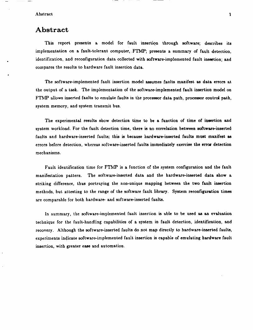
This report presents a model for fault insertion through software; describes i ts

implementation on a fault-tolerant computer, . FTMP; presents a summary of fault detection,

identification, and reconfiguration d a t a collected with software-implemented fault insestion; and

compares the results to hardware fault insertion data.

T h e software-implemented fault insertion model assumes faul ts manifest as d a t a errors at

the output of a task. T h e implementation of the software-implemented fault insertion model on

FTMP allows inserted faults to emulate faults in the processor d a t a path, processor control path,

system memory, and system transmit bus.

T h e experimental results show detection time to be a function of time of insertion and

system workload. For the fault detection time, there is no correlation between softwareinserted

faults and hardware-inserted faults; this is because hardware-inserted faults must manifest as

errors before detection, whereas software-inserted faults immediately exercise the error detection

mechanisms.

Fault identification time for FTMP is a function of the system configuration and the fault

manifestation pattern. The software-inserted da t a and the hardware-inserted d a t a show a

striking difference, thus portraying the non-unique mapping between the two fault insertion

methods, but attesting to the range of the software fault library. System reconfiguration times

are comparable for both hardware- and software-inserted faults.

In summary, the software-implemented fault insertion is able to be used as an evaluation

technique for the fault-handling capabilities of a system in fault detection, identification, and

recovery. Although the software-inserted faults do not map directly to hardware-inserted faults,

experiments indicate software-implemented fault insertion is capable of emulating hardware fault

insertion, with greater ease and automation.

Introduction 2

1. Introduction

Vdidation procedures, such ‘as those proposed in (Carter 86, NASA 79a, NASA 79bj include

steps to characterize and evaluate the behavior of a system under faulty conditions. T h e means

for these evaluations include the following:

1. Computer Simulation: Computer simulation is used to evaluate the manifestation of faults and the system’s response. T h e simulation models range from the Processor- Memory-Switch level through the Instruction-Set-Processor level, the Register- Transfer level, the gate level, and to the device level. T h e drawbacks to simulation are the high cost of model development, computational needs, and the difficulty in model validation [McCough & Stern 81, Rennels 841.

2. Physical Fault Insertion: Physical fault insertion places faults in the hardware of a realized system. T h e advantages over computer simulation include speed and fidelity to actual system faults. T h e drawbacks to this method are two fold. First, fault insertion requires physical manipulation of components, a time consuming effort [Lala & Smith 83aI. Second, the faults are limited to pin level insertion; as realizations moves from SSI/MSI to VLSI, the fault insertion level moves from gate level to system level.

This paper discusses So ftware-Implemented Fault Insertion, in which the at tempt is to

emulate hardware or physical faults by modifying program data or control. T h e motivations for

software-implemented fault insertion include speed and automation advantages over simulation

and physical fault insertion; the experimental run time is near, if not the same, as the actual

system and software-implemented fault insertion does not require any physical manipulation of

system hardware. Additionally, software-inserted faults are repeatable acrocss architectural and

implementation boundaries, since the insertion method does not require detailed information of

hardware implementation. Finally, the gap between pin level fault insertion in VLSI and

software-implemented faults insertion is narrowing and may be approaching equivalence.

T h e literature abounds with prior work demonstrating the benefits of fault insertion and the

feasibility of software-implemented fault insertion at the architectural or bus level; a sampling of I this prior work includes:

0 Pin-level (gate-level) fault insertion has been used in several evaluations including [Decouty e t al. 80, Finelli 87, Lala & Smith 83a, Lala 831. Observations noted in [Lala & Smith 83a, Lala 831 include difficultly caused by incorrect functioning of the

test module with the test equipment attached. From these fault insertion experiments, characterization of fault-handling routines, along with preliminary, but inconclusive d a t a on fault coverage were generated. These experiments demonstrate the value of using fault insertion for fault-tolerant system evaluation.

Introduction 3

0 [Schuette, et al. 861 inserted transient or soft faults in a MC68000 to evaluate software triple-modular redundancy and a signature instruction stream monitor. The MC68000 realization does not allow gate-level fault insertion, hence faults were inserted on the address, da ta , and control bus lines. This experiment shows fault insertion a t the bus level can be used to evaluate fault-tolerance techniques.

0 The Sperry UNIVAC 1100/60 [Boone e t al. 801 has a built-in fault insertion capability to verify fault detection, isolation, and recovery mechanisms. This capability is activated during system idle time and can insert faults in the processor, memory, and 1/0 unit. The UNIVAC 1100/60 system shows fault-tolerant mechanisms can be verified using software control at the system level.

0 (Yang et al. 851 inserted faults into the iAPX 432 to evaluate software-implemented triple-modular redundancy. Faults were inserted by altering bits in the program or d a t a areas of memory using the debugger. The experiment shows fault insertion may be accomplished by altering bits in the memory.

This paper is divided into five sections. The second section gives an overview of the FTMP architecture with emphasis o n the fault-handling mechanisms. Section 3 describes a model for a

fault-tolerant system, a model for fault insertion at the architectural level, and the

implementation of this model on FTMP. Section 4 presents d a t a from software-implemented

fault insertion experiments and provides a comparison, where applicable, to similar hardware

fault insertion experiments. The last section concludes the paper with an evaluation of software-

implemented fault insertion techniques.

FTMP Arch it ec t u re 4

2. FTMP Architecture

This section presents an architectural description of FTMP, the target machine for t h e

sortware-implerric~rited fault insertion. Four subsections include a general overview, followed by a

detailed description of fault detection, fault identification, and fault recovery mechanisms

2.1 General Overview

T h e Fault-Tolerant Multiprocessor, FTMP, is a hardware-redundant multiprocessor

designed for ultrareliable avionic environments [Hopkins et al. 78, Smith & Lala 83, Lala &

Smith 83b). T h e architecture, as seen by the programmer, consists of three virtual processors

with local memory, connected via a common bus to global memory and 1 / 0 ports. Reliability is

attained through hardware redundancy; each virtual processor consists of a processor triad. The

memory and buses are also triplicated. Spare processors, memories and buses shadow (i.e.

execute the same code as) the active units, but d o not participate in voting. Each triad executes

synchronously and a hardware vote occurs during data transfers. Voting is performed by each

receiving unit, either a processor or memory, from data transferred over redundant buses.

T h e bus structure consists of four sets of serial buses, each quintuply redundant, of which

three are active at any time. T h e bus sets are: the Poll Bus, which is the bus arbiter; the

Transmit Bus, which carries address and d a t a information from the processor; the Receive Bus, which carries d a t a from global memory or 1 /0 ports to the processors; and the Clock Bus, which

carries clock signals to each processor to maintain system synchronization.

FThlP employs a realtime operating system with a basic dispatch period of 40 milliseconds,

referred to as R a t e 4 There are two lower rate groups, Rate-3 with a period of 80 milliseconds,

and Rate-1 with a period of 320 milliseconds. Tasks are assigned to rate groups depending upon

the task’s execution requirement; most of the system tasks, such as the system configuration

controller (SCC), a memory checker, status display and self tests are assigned to the lowest rate

group, Rate-1.

FTMP Architecture 5

2.2 Fault Detection

T h e fault detection mechanism for FTMP employs hardware voters residing at the receivers

o f each bus set. A disagreement at the voter sets an error latch associated with the bus line in

error. SCC, running as a Rate-I task, reads the error latches to check for errors and potentially

faulty units. If an error is detected, the time of the error is stored and the fault identification

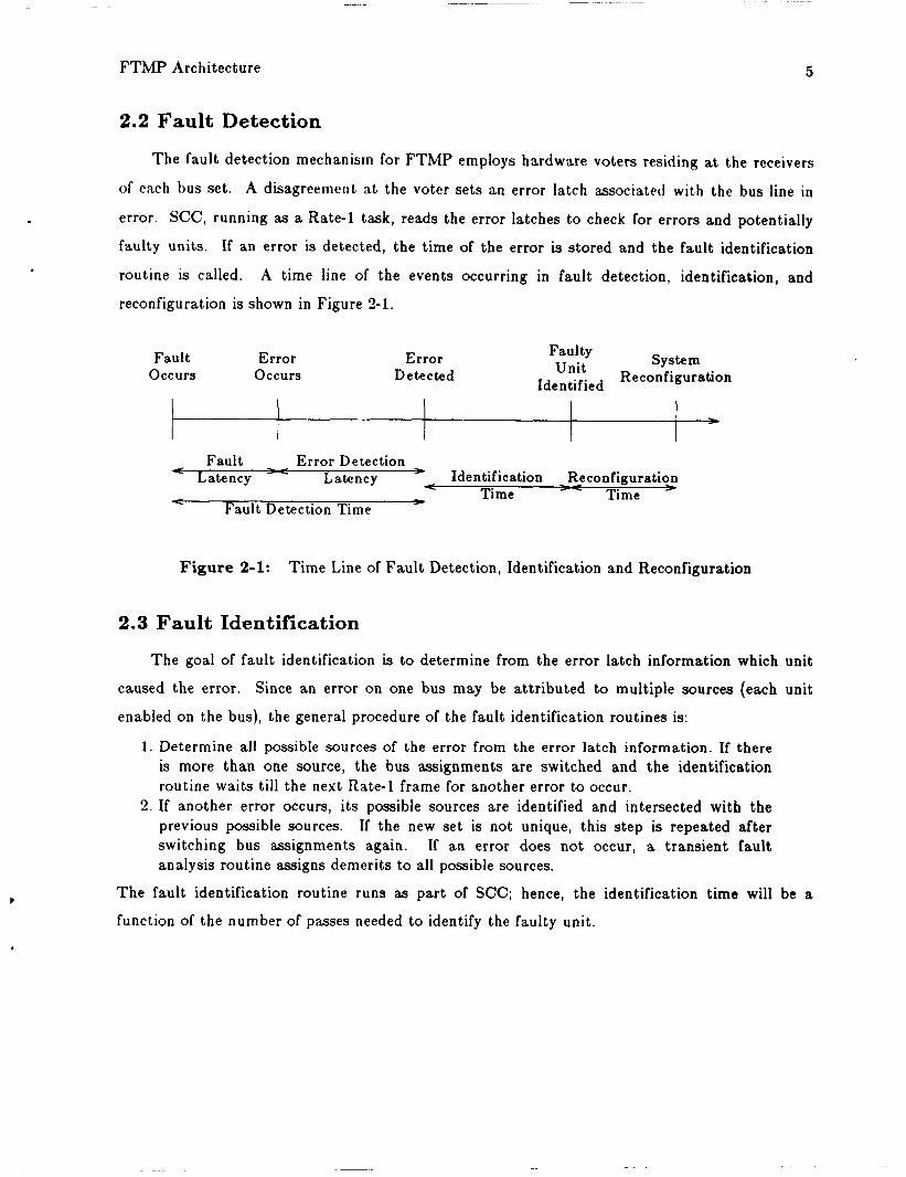
routine is called. A time line of the events occurring in fault detection, identification, and

reconfiguration is shown in Figure 2-1.

Fault Error Occurs Occurs

Error Detected

Faulty

Identified

System Unit Reconfiguration

Fault - Error Detection Latency -- Latency Identification R_econfiguration - -

< t Time Time z- Fault Detection Time

Figure 2-1: Time Line of Faul t Detection, Identification and Reconfiguration

2.3 Fault Identification

T h e goal of fault identification is to determine from the error latch information which unit

caused the error. Since an error on one bus may be attributed to multiple sources (each unit

enabled on the bus), the general procedure of the fault identification routines is:

1. Determine all possible sources of the error from the error latch information. If there is more than one source, the bus assignments are switched and the identification routine waits till the next Rate-1 frame for another error to occur.

2. If another error occurs, i ts possible sources are identified and intersected with the previous possible sources. If the new set is not unique, this s tep is repeated after switching bus assignments again. If an error does not occur, a transient fault analysis routine assigns demerits to all possible sources.

T h e fault identification routine runs as part of SCC; hence, the identification time will be a

function of the number of passes needed to identify the faulty unit.

FTMP Architecture

2.4 System Reconfiguration

The system reconfiguration procedure entails the removal of faulty u n i t s cither by

aclivating a spare u n i t or by graceful degradation. These procedures are described as follows:

1. If there is a spare unit (Processor, Memory, or Bus) and it is shadowing the faulty unit, the bus assignments are changed to bring the spare un i t active and the failed unit inactive.

2. If there is a spare processor or memory and it is shadowing a triad other than the one containing the faulty un i t , then the spare is brought to shadow the triad with the faulty unit, the spare activated and the failed unit deactivated.

3. Finally if there are no spare processors, the triad is retired with i ts good processors assigned as spares. When memories or buses fail without spares, the triad reduces to a duplex.

The Rate-4 dispatcher executes the reconfiguration commands from the information

supplied by the fault identification routine. The reconfiguration time is defined as the time from

fault identification to the execution of the reconfiguration commands.

Implementation 7

3. Software-Implemented Fault Insertion

This section describes a model for a fault-tolerant system, and a model of software-

T h e realization of the software- implemented fault insertion for a realtime operating system.

implemented fault insertion is presented on the example system, FTMP.

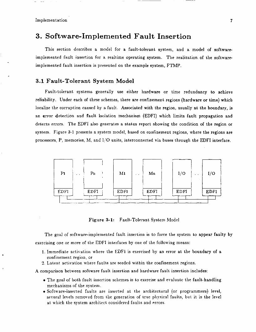
3.1 Fault-Tolerant System Model

Fault- tolerant systems generally use either hardware or time redundancy to achieve

reliability. Under each of these schemes, there are confinement regions (hardware or time) which

localize the corruption caused by a fault. Associated with the region, usually at the boundary, is

an error detection and fault isolation mechanism (EDFI) which limits fault propagation and

detects errors. T h e EDFI also generates a status report showing the condition of the region or

system. Figure 3-1 presents a system model, based on confinement regions, where the regions are

processors, P, memories, 14, and IjO units, interconnected via buses through the EDFI interface.

. .

Figure 3-1: Fault-Tolerant System Model

T h e goal of software-implemented fault insertion is to force the system to appear faulty by

exercising one or more of the EDFI interfaces by one of the following means:

1 . Immediate activation where the EDFI is esercised by an error at the boundary of a

3. Latent activation where faults are seeded within the confinement regions. confinement region, or

A comparison between software fault insertion and hardware fault insertion includes:

0 T h e goal of both fault insertion schemes is to exercise and evaluate the fault-handling mechanisms of the system.

0 Software-inserted faults are inserted a t the architectural (or programmers) level, several levels removed from the generation of true physical faults, but it is the level at. wliich the system architect considered faults and errors.

Implemen tation 8

0 Fault propagation, the spreading of adverse physical phenomena [Laprie 851, is constrained within the fault containment regions, and would be tested by: failure modes and effects analysis, low level physical fault insertion, and simulation.

0 Error propagation, the spreading of errors within the system (Laprie 851, is the primary area which software-inserted faults can be utilized in system evaluation.

0 Software-implemented fault insertion is analogous to functional level testing of hardware or software, which has been shown feasible in the literature (Howdeo 80, Lai 791.

0 The set of faults at the architectural level is more manageable, reduced in size and complexity, than the set of gate level or functional faults.

0 Software-inserted faults may be better in triggering a specific response (such as a malicious liar), which is difficult to generate or reproduce with physical fault insertion.

0 For some desired errors, physical fault insertion may be the easiest method to generate these errors.

0 Physical fault insertion may be more analogous to actual faults generated in the system.

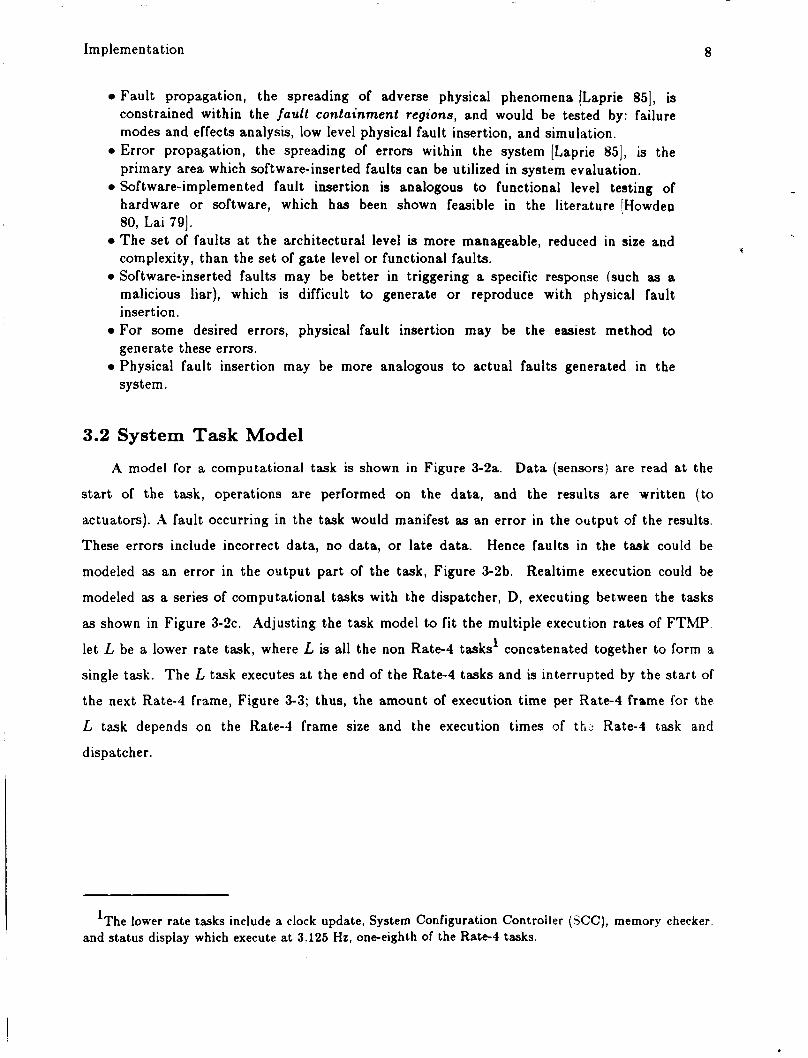
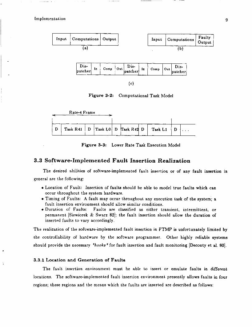
3.2 System Task Model A model for a computational task is shown in Figure 3-2a. Data (sensors) are read at the

s ta r t of the task, operations are performed on the data , and the results are written (to

actuators). A fault occurring in the task would manifest as an error in the output of the results.

These errors include incorrect data , no data , or late data. Hence faults in the t a s k could be

modeled as an error in the oQtput part of the task , Figure 3-2b. Realtime execution could be

modeled as a series of computational tasks with the dispatcher, D, executing between the tasks

as shown in Figure 3-2c. Adjusting the task model to fit the multiple execution rates of FTMP let L be a lower rate task, where L is all the non Rate-4 tasks' concatenated together to form a

single task. The L task executes a t the end of the Rate-4 tasks and is interrupted by the s tar t of

the next Rate-4 frame, Figure 3-3; thus, the amount of execution time per Rate-4 frame for the

L task depends on the Rate-4 frame size and the execution times of the Rate-4 task and

dispatcher.

'The lower rate tasks include a clock update, System Configuration Controller (SCC), memory checker. and status display which execute at 3.125 Hz, one-eighth of the R a t e l tasks.

f

Implementation

Input

9

Computations Output Input Faulty Computations output , I I

(b)

Dis- patcher

- Dis- In Comp Out 'is- In Comp 1 Out

patcher patcher

Figure 3-2: Computational Task Model

D TaskR41 D TaskLO

Rate-4 Frame

D TaskR42 D TaskL1 D . . .

Figure 3-3: Lower Rate Task Execution Model

3.3 Software-Implemented Fault Insertion Realization

T h e desired abilities of software-implemented fault insertion or of any fault insertion in

general are the following:

Location of Fault: Insertion of faults should be able to model true faults which can occur throughout the system hardware. Timing of Faults: A fault may occur throughout any execution task of the system'; a fault insertion environment should allow similar conditions. Duration of Faults: Faults are classified as either transient, intermittent, or permanent [Siewiorek & Swarz 821; the fault insertion should allow the duration of inserted faults t o vary accordingly.

T h e realization of the software-implemented fault insertion in FTMP is unfortunately limited by

the controllability of hardware by the software programmer. Other highly reliable systems

should provide the necessary "hooks " for fault insertion and fault monitoring [Decouty e t al. 80).

3.3.1 Location and Generation of Faults

T h e fault insertion environment must be able to insert or emulate faults in different

locations. T h e software-implemented fault insertion environment presently allows faults in four

regions; these regions and the means which the faults are inserted are described as follows:

Implemen tation

0 Processor Data Path Faults: Faults occurring in the d a t a path may manifest as a number of different error types. These include transmission of incorrect data, no d a t a or late data . T h e software-implemented fault insertion environment assumes processor d a t a path faults manifest as incorrect data being transmitted by the processor, causing an error on the transmit bus assigned to the processor. T h e incorrect d a t a is a single word and the processor s t a t e remains good after the transmission of the bad data . This fault class assumes tha t faults which corrupt multiple words would be detected easier than the single word fault. This generality of this fault class does not limit its application to FTMP.

0 Processor Control Path Faults: Faults within the control path may manifest to many different error types. These include no data transmitted, early or late d a t a transmitted, or incorrect d a t a transmitted. T h e software-implemented fault insertion environment emulates faults within this region by having the processor execute an infinite loop, resulting in no transmission of data . This causes errors on two of the buses to which the processor is assigned: the poll bus because the processor never requests the bus, and the transmit bus because no d a t a is transmitted. Similar emulations of control faults can be used on other systems.

0 System Bus Faults: Faults on a bus may be attr ibuted to many sources, such as noise or a unit transmitting o u t of protocol. Software-implemented fault insertion emulates bus faults by having a processor transmit bad d a t a on a specific bus. Although the processors are generating the errors, the errors map to a particular bus.

10

0 Global Memory Faults: Memory faults may be attr ibuted to decaying bits, stuck-at bits, or incorrect address decoding. Memory faults are emulated by writing bad d a t a into one memory module of a triad, and then performing a read of the location. These type faults are the most general type and can be emulated within other systems.

A few comments on the fault insertion are in order. First, all inserted faults cause an

immediate error; there is no latency between insertion and error occurrence. The present

implementation does not exclude latent faults from further additions. Second, t h e faults are

transient and cause no change in processor s ta te or corruption of data , except for the control

path fault.- Although this is a simplistic model, this is a minimum fault. A faulty processor, or

one with a corrupted s ta te will (most likely) have a stream of incorrect data

r )

2The memory fault is also transient; once the data is changed and read, the memory word is written over.

Implementation 11

3.3.2 Timing of Faults

Faults may occur at any time within the execution of a program. T h e model a s u m e s faults

manifest as errors in the output portion of the task. T h e implementation of software-

implemented fault insertion allows faults to .be generated in the output of Rate-4 application

tasks. T h e occurrence of a fault is specified to a particular Rate-4 frame, but not to the time

within the frame. Furthermore, faults may only occur in Rate-4 application tasks and not

within the dispatcher or lower rate tasks. This limits the insertion time of the faults to specific

tasks.

For FTMP and other hardware-redundant systems, a fault occurring within a task, such as

the dispatcher or the fault-handling routines, would be limited to one of the fault confinement

regions. T h e occurring fault would thus, have no effect on the correct functioning of the other

redundant processor^.^ Additionally the error detection mechanism for FTMP cannot distinguish

the insertion time o r location to a specific task.

3.3.3 Duration of Faults

Faults can be transient (soft), due to a temporary random environmental condition or

permanent (hard), due to a physical change in the hardware. T h e software-implemented fault

insertion environment generates transient faults, and to emulate permanent faults, a transient

fault is repeatedly inserted in consecutive Rate-4 frames. Thus a module with a permanent fault

produces a stream of faulty data , which gives the appearance of a permanent fault when viewed

from the error detection and identification mechanisms.

3.3.4 Workload

A system’s workload is its set of inputs received from its environment; a desirable feature

within any computer evaluation environment is a controllable workload. [Feather e t al.

85) developed a synthetic workload4 generator for FTMP which has been modified to include the

software-implemented fault insertion. T h e synthetic workload provides a means of specificing

the following factors:

3This assumes only single faults, and the absence of simplex data or control.

4A synthetic workload exercises a computer system by modeling its natural workload with generic inputs and tasks.

Implementation 12

0 System Configuration, which defines the number of processor triads and spares. 0 Number of Tasks for each rate group, and the inclusion of the system tasks, such as

0 Workload for each task, which includes the amount of 1/0 and computations per SCC and Sta tus Display.

task.

3.3.5 Recovery Mechanism

To gather a large data base of fault insertion data, a recovery mechanism must augment the

software-impleme'nted fault insertion environment. Draper Labs modified the system

configuration controller to repair and activate processor 3 before fault i n ~ e r t i o n . ~ This repair

code was modified allowing for the repair and activation of the last unit failed (processor,

memory, or bus), before each fault insertion.

3.4 Experimental Environment

T h e experimental environment for software-implemented fault insertion can be divided into

I three sections: the experimental set-up and selection of parameters, the execution of the

experiment and the collection of data , and the analysis of data. This section describes these

areas of the FTMP implementation.

3.4.1 Parameters

T h e first phase of the experimental procedure is experimental setup and selection of

parameters. A program queries the user on the selection of the parameters, and from the inputs,

generates a command file which properly configures FTMP and collects data . T h e controllable

parameters include :

0 Workload: T h e system workload includes the amount and distribution of tasks between the rate groups, the amount of 1 /0 and computation executed by each task, the inclusion of system tasks, and the overall system configuration.

0 Location: T h e different locations for fault insertions are described in Section 3.3.1. 0 Timing: T h e time of fau l t insertion is controlled by the Rate-4 frame, hence a 40

millisecond resolution. 0 Duration: Either a transient (single) fault or a permanent (repeated) fault may be

inserted, as described in Section 3.3.3. 0 Data Collected: T h e d a t a which may be collected includes: the application tasks'

execution time; the fault insertion, detection, identification, and reconfiguration time; the identification of the failed unit; and the reason code for the failure.

'Draper's fault insertion environment inserted faults in Processor 3; before a fault was inserted, the software assured Processor 3 was active in a triad.

Implementation 13

3.4.2 Experimental Execution

T h e second phase of the experimental procedure is insertion of faults and the collection of

data . During each experimental loop the following actions occur:

1. T h e system repairs any module which failed during the last cycle. 2. T h e fault inserter is started and the workload d a t a collection cycle begins. Workload

d a t a (task execution times) are collected for one Rate-1 frame, and the inserted faults trigger the fault-handling mechanisms whose execution times are also collected.

3. T h e requested data is uploaded to the host VAX and the cycle repeated.

T h e cycle time is approximately 30 seconds: one-half is for wait s ta tes between steps one and

two, and steps two and three, which may be reduced by passing ready signals. T h e other half is

consumed during the uploading of the data , which is dependent on the data requested by the

user.

3.4.3 Data Analysis

T h e third phase of the exp rimental pro edure is d a t a analysis. T h e d a t a analysis program

takes the absolute timer values collected from FTMP and records differences between two events

as requested by the user. T h e average, standard deviation, minimum, maximum, and a

histogram of the d a t a are then printed.

I Experiments 14

I I 4. Experiments

With tJic Sol‘t~~src-liii~~lcriit.ii~c~rl Fault lnsertioii Environrnciit iiiiplerneiited, the next s tep

was to run experiments evaluating the feasibility of software-implemented fault insertion, and

the capabilities of the environment. T h e experiments exercised most of the parameters available

in the software-implemented fault insertion environment. In particular the location of the fault,

time of insertion, and system configuration were the primary parameters varied. T h e collection

of d a t a from these experiments involves a measurement of the system workload and the times of

fault insertion, fault detection, identification, and system reconfiguration. Additionally, the unit

which failed and the reason code for the failure were stored for analysis of incorrectly diagnosed

faults. This section details the experiments performed. Comparisons to hardware fault insertion

results [Lala & Smith 83a, Wimmergren 831 are made where appropriate.

4.1 Summary of Draper’s Fault Insertion Data

Draper, unde r contract to h’AS.4, completed extensive hardware fau l t insertion experiments

at the pin (gate) level (Lala & Smith 83a]. Wmmergren [Wimmergren 821 also performed fault

insertion experiments on F T M P for his Master’s research; his results are compared when

appropriate. with the same assumptions as Draper’s da t a . This section summarizes their

experiments and presents a comparison between Draper’s hardware-implemented fault insertion

and the software-implemented fault insertion experiments.

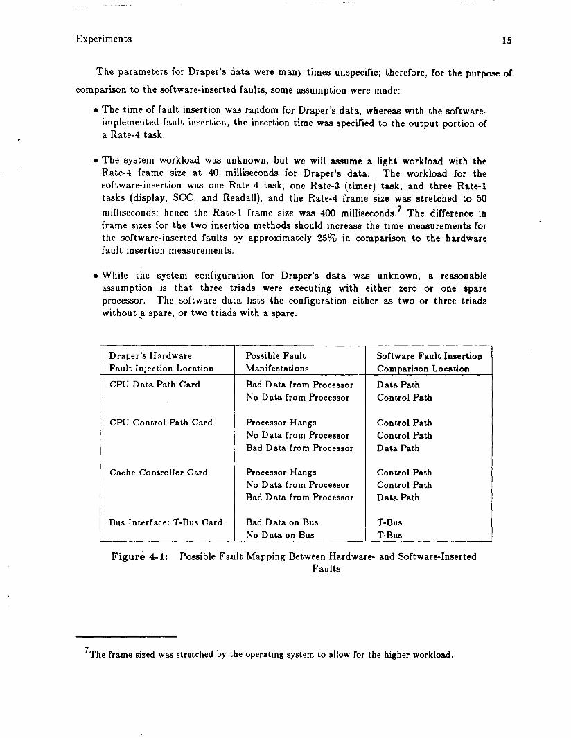
Draper’s esperiments inserted faults at the pin level of the processor; the types of faults

were single stuck-at zero, st.uck-at one, or inverted. T h e d a t a is divided by the fault location,

where the locations are cards i n the LRU’s. For each card, several chips were pulled and faults

inserted on each of the chips. For our comparison, Draper’s d a t a from four different cards were

taken: the CPU d a t a path card (CPUD), the CPU control path card (CPUC), the bus interface

transmit card (BIT), and the cache controller card (CC). These correspond to the software-

implemented fault insertion locations of d a t a path, control path, transmit bus, and data path

respectively; Figure 4-1 diagrams a hypothesized mapping between hardware and software-

inserted faults.

6

GAn LRU is a Line Replaceable LTriit; each is identical and contains a processor, memory and the necessary bus interface circuitry.

~

Experiments 15

T h e parameters for Draper’s d a - a were many times unspecific; therefore, for the purpose of

comparison to the software-inserted faults, some assumption were made:

0 T h e time of fault insertion was random for Draper’s da t a , whereas with the software- implemented fault insertion, the insertion time was specified to the output portion of a Rate-4 task.

0 T h e system workload was unknown, but we will assume a light workload with the Rate-4 frame size at 40 milliseconds for Draper’s data . T h e workload for the software-insertion was one Rate-4 task, one Rate-3 (timer) task, and three Rate-1 tasks (display, SCC, and Readall), and the Rate-4 frame size was stretched to 50 milliseconds; hence the Rate-1 frame size was 400 milliseconds.’ T h e difference in frame sizes for the two insertion methods should increase the time measurements for the software-inserted faults by approximately 25% in comparison to the hardware fault insertion measurements.

0 While the system configuration for Draper’s d a t a was unknown, a reasonable assumption is tha t three triads were executing with either zero or one spare processor. T h e software d a t a lists the configuration either as two or three triads without spare, or two triads with a spare.

D raper’s Hardware Faul t In ie c tion Location CPU Data Path Card

CPU Control Path Card

Cache Controller Card

Bus Interface: T-Bus Card

~~

Possible Fault Manifestations Bad Data from Processor No Data from Processor

Processor Hangs No Data from Processor Bad Data from Processor

Processor Hangs No Data from Processor Bad Data from Processor

Bad Data on Bus No Data on Bus

Software Fault Insertion Comparison Locatioa Data Path Control Path

Control Path Control Path Data Path

Control Path Control Path Data Path

T-BUS T-BUS

Figure 4-1: Possible Fault Mapping Between Hardware- and Software-Inserted Faults

7The frame sized was stretched by the operating system to allow for the higher workload.

Experimen ts 16

4.2 Fault Detection Time Fault detection time is the time from the insertion of a fault until an error is detected by

the system. For software-inserted fault, the insertion time is at the end of a specified task,

whereas with Draper’s hardware-inserted faults, the insertion times are any point within the

frame. Hence the

detection time for software-inserted faults should be a maximum of one Rate-1 frame (400

milliseconds), the latency in reading the error latches. For hardware-inserted faults the detection

time will include the manifestation of the fault as an error, along with the delay in reading the

error latch, tha t is, fault latency plus error detection latency.

Error detection, reading of the error latches, is done by SCC a t Rate-1.

In predicting the detection time for software-inserted faults, the following parameters

affecting the detection time are proposed:

0 Workload: A large workload stretches the frame size, placing the detection point later in the frame. Likewise, a large workload limits the execution time per Rate-4 frame of the lower rate tasks (e.g. error detection). The workload function is expressed by R4task, the Rate-4 task size, and R4Frs i ze , the Rate-4 frame mize, both measured in milliseconds.

0 Time of error detection: The point at which error detection occurs within the realtime cycle affects the error detection latency. This time within the realtime Rate-1 cycle is determined by the amount of time which the lower rate task executes before the error detection routine is run. This time is represented as LDet and is measured in milliseconds.

0 Time of Insertion: The of point of fault insertion within the realtime cycle in conjunction with the time of error detection governs the fault detection latency. T h e time of insertion is represented as Tin and measured in Rate-4 frames.

Finally, let: L x T i m e be defined as the amount of time tha t the lower rate tasks execute per

frame, where LzTime=max (R4FrmSire-R4Task ,10) milliseconds, where 10 millisecond is

the amount of time the dispatcher will allow for the execution of lower rate tasks. The error

detection time can be represented by: LDe t

L x T i m e D e t T i m e = R 4 F r m S i z e X [[( ) - Tin] mod 81

~~

The quotient in Equation (4.1) marks the Rate-4 frame in which the error detection task runs;

the modulo 8 term comes from the realtime cycle of F T M P (eight Rate-4 frames per Rate-1

frames).

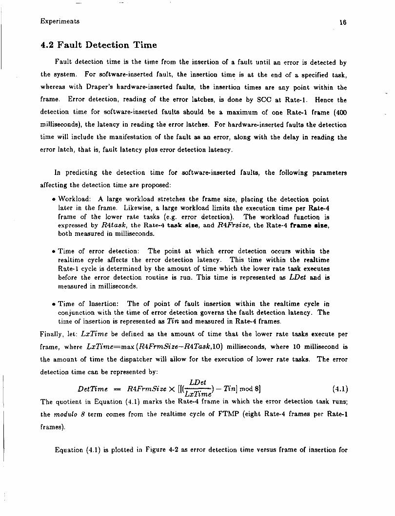
Equation (4.1) is plotted in Figure 4-2 as error detection time versus frame of insertion for

Experiments 17

different workloads; two experimental runs of software-inserted faults are also plotted. In Figure

4-2, one Rate-] cycle, consisting of eight Rate-4 frames, is plotted twice to slio\\i the contiiiuity

of the error detection time i n the realtime cycle. T h e high worklo3d da ta has a Rate-4 frame

size of 50 milliseconds and the low workload d a t a a 40 millisecond friulle size. In comparing the

d a t a of Figure 4-2, the experimental d a t a corresponds closely to the computed data. T h e reason

for the multiple d a t a points for each insertion time is tha t error detection can be accelerated or

delayed one Rate-4 frame cycle, due to the run time task allocation of FTMP. T h e increase in

the slope as the workload increases is due to the lengthening of the basic frame size, hence

placing the error detection a further time away from the fault insertion.

500 1 a\

Detect.ion Time DEtTinie

t

Experimental High Workload n Experimental Low Workload

-Equation 4.1, High Workload - -Equation 4.1, Low Workload

100 -4 ;-. 3 D

B 0

0 I I I I I 0 2 4 6 0 2

Fault Insertion Time, Titi (Frame Number)

Figure 4-2: Error Detection Time as a Function of Insertion Time

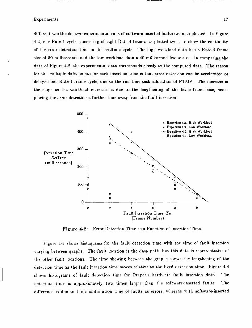
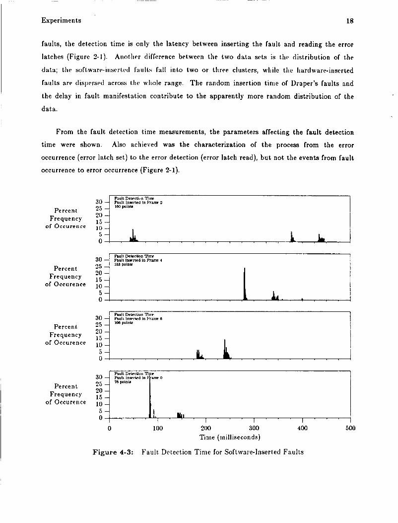
Figure 4-3 shows histograms for the fault detection time with the time of fault insertion

varying between graphs. T h e fault location is the d a t a path, but this d a t a is representative of

the other fault locations. T h e time skewing between the graphs shoivs the lengthening of the

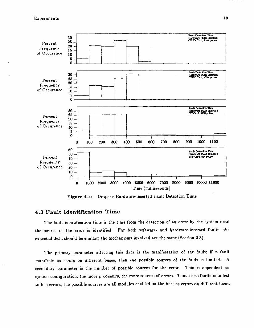
detection time as the fault insertion time moves relative to the fixed detection time. Figure 4-4

shows histograms of fault detection time for Draper’s hardware fault, insertion data . The

detection t ime is approximately two times larger than the software-inserted faults. The

difference is due to the manifestation time of faults as errors, wliereas with software-inserted

Experiments

30 - 35 - ?O - 15 -

of Occurence 10 - 5 - 0 ,

Percent Frequency

18

h u l l DetecUon ‘llm Fault Invrted In F T ~ 4 lupolnu

r 7 . . . . r r . , & . A . t . . .

faults, the detection time is only the latency between inserting the fault and reading the error

latches (Figure 2-1). Anotlier difference between the two d a t a sets is tlrc. distribution of thc

data; the soltwarc.-itiscrl,c.(l fiiIIItS fidI into two or three clusters, while tlie hartlwarc-iiiscrted

faults are dispersed across tlic wllole range. T h e random insertion time of Draper’s faults and

the delay in fault manifestation contribute to the apparently more random distribution of the

data .

10

From the fault detection time measurements, the parameters affecting the fault detection

time were shown. Also achieved was the characterization of the process from the error I occurrence (error latch set) to the error detection (error latch read), but not the events from fault

occurrence to error occurrence (Figure 2-1).

of Occurence -

I I r r I 1 r I , , , , , L a ,

r mu11 Detection nnr Fault lnsrrlcd In R a m 0 2 4 100 poinu

Percent ?O - Frequency 15 -

of Occurence lo - 5 -

i

Percent Frequency

of Occurence

Figure 4-3: Fault Detection Time for Software-1nsert.ed Faults

Experiments

20 - 15 - 10 - 5 -

19

-- Percent Frequency

of Occurence

30 - Percent 25-

20 - Frequency - of Occurence 10 -

5

25 30 A

Fault Deteeuoo nm Hudrva Fruit hkcUon CHJC Cud. i701 polnu -m

n

Fu~ItDa@cUonTlrm Hard- hull InJeaIon C C ~ d ~ p o l n n

1

1

30 - 25 - 20 - 15 - 10 - 5 -

1 1 I

_ _ Frequency 30 -

of Occurence 20 - 10 - 0 L I I 2

I I I I I I I

o ! I I I I I

Pe rce n t Frequency

of Occurence

-- I

50 j-i Percent 40

4.3 Fault Identification Time

T h e fault identification time is the time from the detection of an error by the system until

For both software- and hardware-inserted faults, the the source of the error is identified.

expected data should be similar; the mechanisms involved are the same (Section 2.3).

T h e primary parameter affecting this d a t a is the manifestation of the fault; if a fault

manifests as errors on different buses, then the possible sources of the fault is limited. A

secondary parameter is the number of possible sources for the error. This is dependent on

system configuration: the more processors, the more sources of errors. T h a t is: as faults manifest

to bus errors, the possible sources are all modules enabled on the bus; as errors on different buses

I Experiments 20

I occur from the same faulty source then the bus error "signature" will map to fewer modules.

The experiments conducted varied the fault locations (manifestation), and the system

configuration (possible sources).

I

The d a t a should be grouped according to the execution time of the identification routine, I I which is dependent on the number of suspect units. The routine runs as a R a t e l task, once per

400 milliseconds, with the d a t a grouped according to the number of passes.

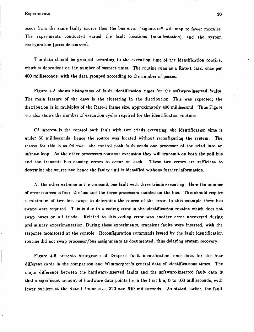
Figure 4-5 shows histograms of fault identification times for the softwareinserted faults.

The main feature of the d a t a is the clustering in the distribution. This was expected; the

distribution is in multiples of the Rate-1 frame size, approximately 400 millisecond. Thus Figure

4-5 also shows the number of execution cycles required for the identification routines.

Of interest is the control path fault with two triads executing; the identification time is

under 50 milliseconds, hence the source was located without reconfiguring the system. The

reason for t h i s is as follows: the control path faul t sends one processor of the triad into an

infinite loop. As the other processors continue execution they will transmit on both the poll bus

and the transmit bus causing errors to occur on each. These two errors are sufficient to

determine the source and hence the faulty unit is identified without further information.

At the other extreme is the transmit bus fault with three triads executing. Here the number

of error sources is four, the bus and the three processors enabled on the bus. This should require

a minimum of two bus swaps to determine the source of the error. In this example three bus

swaps were required. This is due to a coding error in the identification routine which does not

swap buses on all triads. Related to this coding error was another error uncovered during

preliminary experimentation. During these experiments, transient faults were inserted, with the

response monitored at the console. Reconfiguration commands issued by the fault identification

routine did not swap processor/bus assignments as documented, thus delaying system recovery.

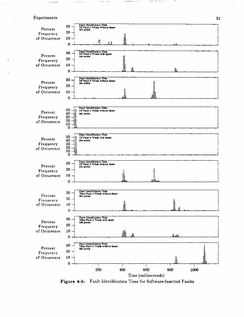
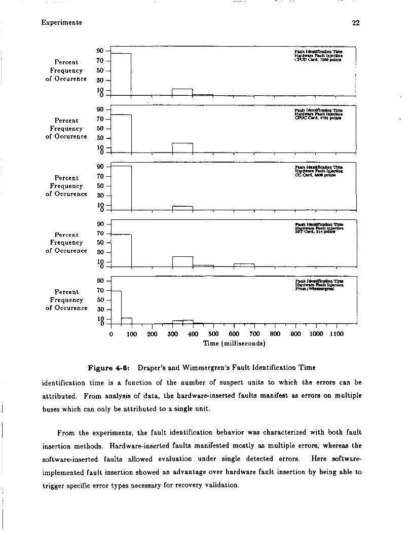
Figure 4-6 presents histograms of Draper's fault identification time d a t a for the four

different cards in the comparison and Wimmergren's general d a t a of identifications times. The

major difference between the hardware-inserted faults and the software-inserted fault da t a is

that a significant amount of hardware da t a points lie in the first bin, 0 to 100 milliseconds, with

fewer outliers a t the Rate-1 frame size, 320 and 640 milliseconds. As stated earlier, the fault

Experiments

30 - 20 -

21 Fault Identination l lme DP h u l t 2 M a d s without Spare 47s polnu Percent

Frequency of Occurence

3O - 30 - 10 -

Percent Frequency

of Occurence

Fault IdentifluDon llm DP Fault 2 Rlds with Spm 440 polno

Percent Frequency

of Occurence

30 - 20 - 10 - 0 - .

Percent Frequency

of Occurence

- Fault IdenUfluUon nm DP h u l t 3 ' N d r withouc Spare 466 polno

. .

Percent Frequency

of Occurence

-

20 - 10 -

Percent Frequency

of Occurence

Fault IdenUIlatloa llm 'IBur Fault 2 Trlada wltbout Spare am polnu

...

Pe rce n t Frequency

of Occurence

30 - 20 - 10 -

Percent Frequency

of Occurence

Fault Identination nm l€bMF.ult2MadawlthSpue 6C8 polnb

Anfill

Percent Frequency

of Occurence

30 -' 20 -

Fault Identlnatlon Tlme l€bM Fault 3 Trlada wlthout Spare 968 polno

Fault Identlnation Tme 8 Fault 2 Rlada wtth Sue E40 polno

30 i

2o 10 Allh

Figure 4-5: Fault Identification Time for Software-Inserted Faults

Experiments

90 -

Frequency 50 - of Occurence 30-

Percent 70 -

‘8 -

22

Fault I d e ~ u n ~ o n ?ha H u d w u e hl l InJeetlon GVD Qld. 72Ul polnu

I I 1 , 1 ! I I I I

10 4

Percent Frequency 50

of Occurence 30

90 - Percent 70

Frequency 50 - of Occurence 30 -

I

Furl8 IbanlUlc.0on llna H u d r v s Rull InJecUon

1M-l -7

‘ 8 ~ ~ , , 1 ; ~ ~ 1 , , , 1 , 1 , , , 1 , , , , .

Frequency 50 of Percent Occurence 7-l 30

1Q-4 I - I

Percent 70

of Occurence 30 Frequency 504 I

Figure 4-6: Draper’s and Wimmergren’s Fault Identification Time

identification time is a function of the number of suspect units to which the errors can be

attributed. From analysis of data , the hardware-inserted faults manifest as errors on multiple

buses which can only be attributed to a single unit.

From the experiments, the fault identification behavior was characterized with both fault

insertion methods. Hardware-inserted faults manifested mostly as multiple errors, whereas the

software-inserted faults allowed evaluation under single detected errors. Here software-

implemented fault insertion showed an advantage over hardware fault insertion by being able to

trigger specific error types necessary for recovery validation.

Experimen ts 23

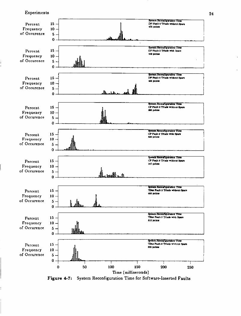
4.4 System Reconfiguration Time

T h e system reconfiguration time is the time from the identification of a faulty unit to the

time when the unit is removed from the active system. T h e d a t a for software-inserted faults

should be similar to Draper’s hardware-inserted faults. The primary parameter is the system

configuration, the presense or absence of spares. The d a t a should show an increase in system

reconfiguration time when spares are not available.

Figure 4 7 shows histograms of system reconfiguration times under various system

configurations and fault locations. With the d a t a path and control path faults, the failed unit

was a processor and hence the processor was retired; for the transmit bus fault a bus was marked

faulty and replaced. T h e d a t a show the expected increase in reconfiguration time when no

spares are available, furthermore the d a t a is clustered at 45 and 95 milliseconds. This represents

the period of the dispatcher which executes the reconfiguration commands.

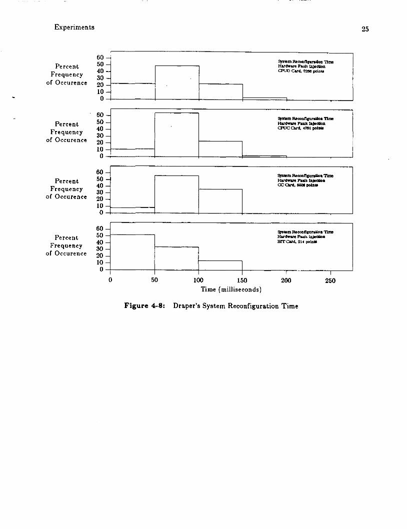
Figure 4 8 shows Draper’s system reconfiguration data . Their d a t a is similar to the sum of

the software-inserted fault data . Draper’s d a t a lacks the resolution and specification of

experimental conditions for useful comparisons, but from the two d a t a sets, i t is evident

software-implemented fault insertion can be used to characterize and evaluate the fault recovery

procedures of a system.

\

Percent 15 -

a8n polnta Percent 15

Frequency 10 of Occurence 5

0

* y r c e m R l c o n n ~ n ~ BFul l t 2 MaiJ r t c b spM am polrib

Percent 15 - Frequency 10 -

of Occurence 5 - 0

"7 polntl Percent 15

Frequency 10 of Occurence 5

0

Syalcm Reconn#urulon nm DP h u l t 2 Rlad8 wlcb Spve 440 polntr

Percent 15 - Frequency 10 -

of Occurence 5 - 0

Wkrn ~ e c o n n ~ u r . u o ~ nm

ar, polntl lBUa Wt 8 Mad8 without SpM

1

I ~ " ~ I " ' ' I ' 1 . J

Experiments

60 -' 50 - 40 - 30 -

of Occurence 20 - 10 - 0 ,

Percent Frequency

25

*ern Reconnmdon nm H v d w v e FUJI$ InJedon CSWD Cud 721M polnu

1

10 '

60 -/

60 -

40 - Percent 50 - Frequency 3o -

of Occurence 20- 10 -, 0 ,

30 of Occurence 20

Percent Frequency

SylornReewflgurrUonllmt Hardware Fault InJearOn oz a d , aaa poho

10 - 0 1 ! I

Percent Frequency 3o

of Occurence 20

0 50 100 150 200 250 Time (milliseconds)

Figure 4 8 : Draper's System Reconfiguration Time

Conclusions 26

5. Conclusions

This paper presented a model for software-implemented fault insertion and its

implementation on a fault-tolerant computer, FTMP. Experiments were conducted to compare

the software-implemented fault insertion to hardware fault insertion in the characterization of

fault detection, identification, and recovery. From the experiments, the following information

regarding the two fault insertion methods can be asserted:

0 Both fault insertion schemes were able to characterize the fault detection, identification, and recovery times of the system.

0 Hardware fault insertion places the fault at a lower level (pin level) than the software-insertion (processor level). For this reason, the detection times for the hardware-inserted faults included the fault latency times, whereas software- implemented fault insertion only included the error detection latency, Figure 2-1.

0 T h e fault manifestation and propagation for hardware-inserted faults allows less control in the generation of specific error types than the software-inserted faults. This control was available with the software-implemented fault insertion, and was useful in discovering a bug in one of the fault-handling routines.

In summary, although software-implemented fault insertion does not fullp emulate hardware

fault insertion, i t provides a means to evaluate the fault detection, identification, and recovery

means of a system, and in some aspects provides better regulation in generating specific errors in

the system. T h e software-implemented fault insertion can also be used for system

characterization across architectural and implementation boundaries with greater ease and

automation than hardware fault insertion. Furthermore, as the controllability and observability

of systems decrease due to the increased use of VLSI technology, software-implemented fault

insertion may be a reasonable approach to system evaluation.

Appendix 27

Appendix A. Source Files This appendix lists the source and executable files on the NASA VAX, System 10, which are

used by the Software-Implemented Fault Insertion Environment. A brief explanation is given for

each file listed.

A.l FTMP Files

T h e directory containing the F T M P AED source files is dlsk$MO : Ccmu . aedl ; these files

can also be found in dlsk$MO : Cewc . swf I. wrkld. aedl .

0 swf 1. aed: contains the procedure swf 1 0 which inserts the faults into FTMP tasks.

0 nf scc . aed: is a modified version of the system configuration controller, FSCC, capable of repairing any specific Processor, Memory or Bus.

0 fwrkld44.aed: is the control task which starts the fault insertion and data collection cycle.

0 fwrkld4.aed: contains the Rate-4 FTMP workload tasks; these tasks call the swf i 0 procedure.

0 fwrkld3. aed: contains the Rate-3 FTMP workload tasks. 0 fwrkldl . aed: contains the Rate-1 FTMP workload tasks. 0 fwrkld. asm: contains the system memory tables for FTMP. This file is located in

the directory dlsk$MO : Ccmu . asm] .

A.2 Data Collection and Analysis Files

T h e directory containing the d a t a collection and analysis programs for the

So ftware-Implemented Fault Insertion Environment is dlsk$MO : Cewc . swf 1. wrkld . code]. 0 wrkld. c, wrkld. exe: generates the command files which configure FTMP for the

0 anal. c, anal. exe: analyzes the collected data and prints user-requested

0 btree .c: has the binary tree code used for holding d a t a during processing by

0 def lnes . h: contains global definitions for both wrkld. c and anal. c.

experiment and collect d a t a from F T M P during experiment.

information regarding the data.

anal. c. btree . c is complied and then linked with anal. c to form anal. exe.

1 References 28

I References

[Boone e t al. 801 L.A. Boone, H.L. Liebergot, and R.M. Sedmak. Availability, Reliability, and Maintainability Aspects of the Sperry UNIVAC

In 10th International Symposium on Fault-Tolerant Computing, pages 3-9. 1100/60.

IEEE, June, 1980.

[Carter 861 W.C. Carter. System Validation - Putting the Pieces Together. In 7th AIAA/IEEE Digital Avionics Systems Conference, pages 687-694.

1986.

[Decouty e t al. 801 B. Decouty, G. Michel, C. Wagner. An Evaluation Tool of Faul t Detection Mechanisms Efficiency. In 10th International Symposium on Fault-Tolerant Computing, pages

225-227. IEEE, June, 1980.

[Feather e t al. 851 Frank Feather, Daniel Siewiorek, and Zary Segall. Validation of a Fault-Tolerant Multiprocessor: Baseline Ezperiments and

Technical Report CMU-CS-85-145, Carnegie Mellon University, July, 1985. Workload Implementation.

I [Finelli 871 George B. Finelli.

Characterization of Fault Recovery through Fault Injection on FTMF'. IEEE Transactions on Reliability R-36(2):161-170, June, 1987.

[Hopkins et al. 781 A.L. Hopkins, T.B. Smith, and J.H. Lala. F T M P - A Highly Reliable Multiprocessor. Proceeding of the IEEE 66(10):1221-1237, October, 1978.

[Howden SO] William E. Howden. Functional Program Testing. IEEE Transactions on So ftware Engineering SE6(2):162-169, March, 1980.

[Lai 791 Larry Kwok-Woon Lai. Error-Oriented Architecture Testing. In National Computer Conference, pages 565-576. June, 1979.

I

[Lala 83) 3.H. Lala. Fault Detection, Isolation, and Reconfiguration in FTMP: Methods and

In 5th IEEE/AIAA Digital Avionics Systems Conference, pages 21.3.1-21.3.9. Experimental Results.

November, 1983.

References 29

[Lala & Smith 83al Jaynarayan H. Lala and T. Basil Smith 111. Development a n d Evaluation of a Fault-Tolerant Multiprocessor Computer,

Vol. III, FTMPTest and Evaluation .

Charles Stark Draper Laboratories, 1983. NASA CR-166073.

[Lala & Smith 83b] Jaynarayan H. Lala and T. Basil Smith 111. Development and Evaluation of a Fault-Tolerant Multiprocessor Computer,

Charles Stark Draper Laboratories, 1983. Vol. 11, FTiVfP Soft ware

NASA CR-166072.

[Laprie 85) Jean- Cluade Lap r ie . Dependable Computing and Faul t Tolerance: Concepts and Terminology. In 15th International Symposium on Fault-Tolerant Computing, pages 2-1 1.

1985.

[McGough & Stern 811

[NASA 79a]

[NASA 70b)

(Rennels 8.11

[Schuette, e t al.

John-G. McGough and Fred L. Swern. Measurement o f Fault Latency in a Digital Avionic Mini Processor Bendix Corp., 1981. NASA CR-3462.

NASA-Langley Research Center. Validation Methods for Fault-Tolerant Avionics and Control Systems -

Working Croup Meeting I , NASA-Langley Research Center, 1979. NASA CP-3114.

Research Triangle Institute. Validation Methods for Fault-Tolerant Avionics and Control Systems .-

Working Croup Meeting II, NASA-Langley Research Center, 1979. NASA CP-2130.

David A. Rennels. Fault-Tolerant Computing - Concepts and Examples. I E E E Transactions on Computers C-33( 12):1116-1129, 1984.

361 M.A. Schuette, J .P. Shen, D.P. Siewiorek, and Y.X. Zhu. Experimental Evaluation of Two Concurrent Error Detection Approaches. In 16th International Symposium on Fault-Tolerant Computing, pages

138-143. IEEE, July, 1986.

[Siewiorek & S w a n 821 Daniel P . Siewiorek and Robert S. Swarz. The Theory a n d Practice of Reliable System Design. Digital Press, 1982.

References 30

[Smith & Lala 83) T. Basil Smith I11 and Jaynarayan H. Lala. Development and Evaluation o f a Fault-Tolerant Multiprocessor Computet,

Vol. I, FTMP Rinciples of Operat ions Charles Stark Draper Laboratories, 1983. NASA CR- 16607 1.

, [Wimmergren 821 I Alan Lee Wimmegren.

Verification of a Faul t Tole rant Mu1 t i-Processor Arc hi tec t ure. Master’s thesis, Massachusetts Institute of Technology, May, 1982. CSDL-T-782.

(Yang e t al. 851 X.Z. Yang, G. York, W.P. Birmingham, and D.P. Siewiorek Faul t Recovery of Triplicated Software on the Intel iAPX 432. In Distributed Computing Systems, pages 438443. May, 1985.

.

Report Documentation Page 1. Report No.

NASA CR- 178423

2. Government Accession No.

4. Title and Subtitle

Software-Implemented F a u l t I n s e r t i o n : An FTMP Example

19. Securii Classif. (of this report)

7. Authorb)

20. Security Classif. (of this page) 21. No. of pages 22. Price

Edward W . Czeck, Daniel P. Siewiorek, and Zary Z. Segal l

9. Performing Organization Name and Address

Carnegie-Me1 1 on U n i v e r s i t y Geud.l.irllent ur" E l e c t r i c a l and Computer Engineer ing P i t tsburgh, PA 15213

Nat iona l Aeronautics and Space Admini s t r a t i on !,lashinaton, DC 20546-0001

12. Sponsoring Agency Name and Address

15. Supplementary Notes

3. Recipient's Catalog No.

5. Report Date

October 1987

6. Performing Organization Code

8. Performing Organization Report No.

10. Work Unit No.

505-66-21-01 11. Contract or Grant No.

NAG1 - 190

13. Type of Report and Period Covered

Contractor Report 14. Sponsoring Agency Code

Langley Technical Monitor: George B. F i n e l l i

16. Abstract

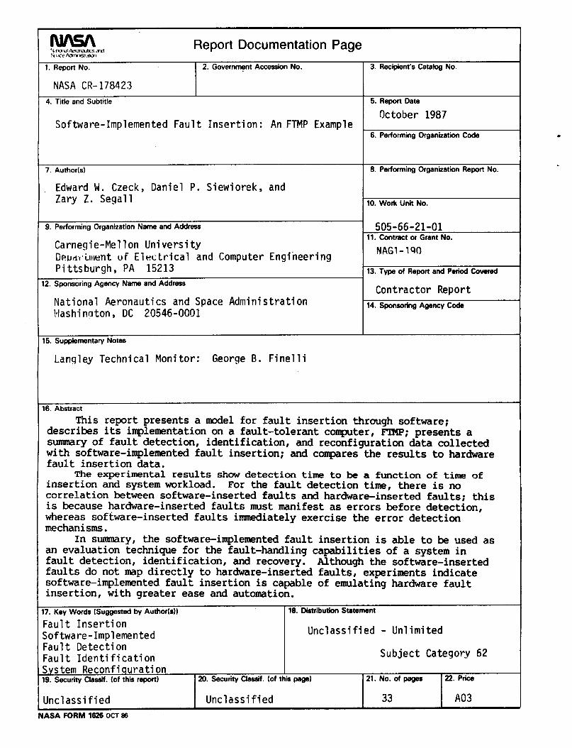
This report presents a model for fault insertion through software; describes its implementation on a fault-tolerant computer, FTMP; presents a summary of fault detection, identification, and reconfiguration data collected with software-implemented fault insertion; and compares the results to hardware fault insertion data.

The experimental results show detection time to be a function of time of insertion and system workload. For the fault detection time, there is no correlation between software-inserted faults and hardware-inserted faults; this is because hardware-inserted faults must manifest as errors before detection, whereas software-inserted faults immediately exercise the error detection mechanisms . an evaluation technique for the fault-handling capabilities of a system in fault detection, identification, and recovery. Although the software-inserted faults do not map directly to hardware-inserted faults, experiments indicate software-implemented fault insertion is capable of emulating hardware fault insertion, with greater ease and automation.

In summary, the software-implemented fault insertion is able to be used as

I 18. Dmribution Statement 17. Key Worda (Suggested by Author(s1)

Fau l t I n s e r t i o n Software-Implemented F a u l t Detect ion F a u l t I d e n t i f i c a t i o n

I Unc lass i f i ed - Un l im i ted

Subject Category 62

Uncl ass i f i ed I Unc lass i f i ed I 33 1 A03 I I I

IASA FORM 1626 OCT 86