software engineering for embedded systems || optimizing embedded software for performance

CHAPTER 11

Optimizing Embedded Software forPerformance

Robert Oshana

Chapter Outline

The code optimization process 314

Using the development tools 314Compiler optimization 315

Basic compiler configuration 316

Enabling optimizations 316

Additional optimization configurations 317

Using the profiler 317

Background � understanding the embedded architecture 317Resources 317

Basic C optimization techniques 318Choosing the right data types 318

Use intrinsics to leverage embedded processor features 318

Functions Calling conventions 319

Pointers and memory access 321

Ensuring alignment 321

Restrict and pointer aliasing 322

Loops 324

Communicating loop count information 324

Hardware loops 324

Additional tips and tricks 326

Memory contention 326

Use of unaligned accesses 326

Cache accesses 326

Inline small functions 326

Use vendor run-time libraries 327

General loop transformations 327Loop unrolling 327

Background 327

Implementation 328

Multisampling 328

Background 328

Implementation procedure 329

313Software Engineering for Embedded Systems.

DOI: http://dx.doi.org/10.1016/B978-0-12-415917-4.00011-6

© 2013 Elsevier Inc. All rights reserved.

http://dx.doi.org/10.1016/B978-0-12-415917-4.00011-6

Implementation 329

Partial summation 329

Background 329

Implementation procedure 331

Implementation 331

Software pipelining 331

Background 331

Implementation 331

Example application of optimization techniques: cross-correlation 333Setup 334

Original implementation 334

Step 1: use intrinsics for fractional operations and specify loop counts 336

Step 2: specify data alignment and modify for multisampling algorithm 336

Step 3: assembly-language optimization 338

The code optimization process

Prior to beginning the optimization process, it’s important to first confirm functional

accuracy. In the case of standards-based code (e.g., voice or video coder), there may be

reference vectors already available. If not, then at least some basic tests should be written to

ensure that a baseline is obtained before optimization. This enables easy identification that

an error has occurred during optimization � incorrect code changes done by the

programmer or any overly aggressive optimization by a compiler. Once tests in place,

optimization can begin. Figure 11.1 shows the basic optimization process.

Using the development tools

It’s important to understand the features of the development tools as they will provide many

useful, time-saving features. Modern compilers are increasingly better performing with

embedded software and leading to a reduction in the development time required. Linkers,

debuggers and other components of the tool chain will have useful code build and

debugging features, but for the purpose of this chapter we will focus only on the compiler.

Build Generatetests

Optimize Checkoutputs

Figure 11.1:Basic flow of optimization process.

314 Chapter 11

Compiler optimization

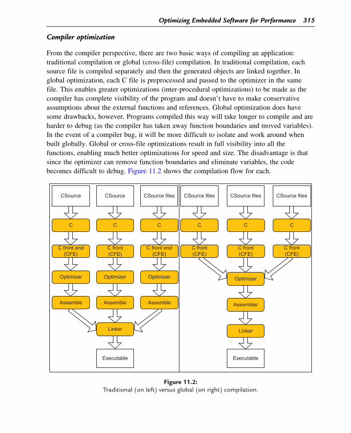
From the compiler perspective, there are two basic ways of compiling an application:

traditional compilation or global (cross-file) compilation. In traditional compilation, each

source file is compiled separately and then the generated objects are linked together. In

global optimization, each C file is preprocessed and passed to the optimizer in the same

file. This enables greater optimizations (inter-procedural optimizations) to be made as the

compiler has complete visibility of the program and doesn’t have to make conservative

assumptions about the external functions and references. Global optimization does have

some drawbacks, however. Programs compiled this way will take longer to compile and are

harder to debug (as the compiler has taken away function boundaries and moved variables).

In the event of a compiler bug, it will be more difficult to isolate and work around when

built globally. Global or cross-file optimizations result in full visibility into all the

functions, enabling much better optimizations for speed and size. The disadvantage is that

since the optimizer can remove function boundaries and eliminate variables, the code

becomes difficult to debug. Figure 11.2 shows the compilation flow for each.

CSource CSource CSource files CSource files CSource files CSource files

C

C front end(CFE)

C front end(CFE)

C front(CFE)

C front(CFE)

C front(CFE)

C front(CFE)

C C C C C

Optimizer Optimizer Optimizer Optimizer

Assemble Assemble Assemble Assembler

Linker

Executable Executable

Linker

Figure 11.2:Traditional (on left) versus global (on right) compilation.

Optimizing Embedded Software for Performance 315

Basic compiler configuration

Before building for the first time, some basic configuration will be necessary. Perhaps the

development tools come with project stationery which has the basic options configured, but

if not, these items should be checked:

• Target architecture: specifying the correct target architecture will allow the best code to

be generated.

• Endianness: perhaps the vendor sells silicon with only one edianness, perhaps the

silicon can be configured. There will likely be a default option.

• Memory model: different processors may have options for different memory model

configurations.

• Initial optimization level: it’s best to disable optimizations initially.

Enabling optimizations

Optimizations may be disabled by default when no optimization level is specified and either

new project stationery is created or code is built on the command line. Such code is

designed for debugging only. With optimizations disabled, all variables are written and read

back from the stack, enabling the programmer to modify the value of any variable via the

debugger when stopped. The code is inefficient and should not be used in production code.

The levels of optimization available to the programmer will vary from vendor to vendor,

but there are typically four levels (e.g., from zero to three), with three producing the most

optimized code (Table 11.1). With optimizations turned off, debugging will be simpler

because many debuggers have a hard time with optimized and out-of-order scheduled code,

but the code will obviously be much slower (and larger). As the level of optimization

increases, more and more compiler features will be activated and compilation time will be

longer.

Note that typically optimization levels can be applied at the project, module, and function

level by using pragmas, allowing different functions to be compiled at different levels of

optimization.

Table 11.1: Example optimization levels for an embedded optimizing compiler.

Setting Description

O0 Optimizations disabled. Outputs un-optimized assembly code.O1 Performs target-independent high-level optimizations but no target-specific optimizations.O2 Target independent and target-specific optimizations. Outputs non-linear assembly code.O3 Target independent and target-specific optimizations, with global register allocation. Outputs

non-linear assembly code. Recommended for speed-critical parts of application.

316 Chapter 11

Additional optimization configurations

In addition, there will typically be an option to build for size, which can be specified at any

optimization level. In practice, a few optimization levels are most often used: O3 (optimize

fully for speed) and O3Os (optimize for size). In a typical application, critical code is

optimized for speed and the bulk of the code may be optimized for size.

Using the profiler

Many development environments have a profiler, which enables the programmer to

analyze where cycles are spent. These are valuable tools and should be used to find the

critical areas. The function profiler works in the IDE and also with the command line

simulator.

Background � understanding the embedded architecture

Resources

Before writing code for an embedded processor, it’s important to assess the architecture

itself and understand the resources and capabilities available. Modern embedded

architectures have many features to maximize throughput. Table 11.2 shows some features

that should be understood and questions the programmer should ask.

Table 11.2: Embedded architectural features.

Instruction setarchitecture

Native multiply or multiply followed by add?Is saturation implicit or explicit?Which data types are supported � 8, 16, 32, 40?Fractional and/or floating point will be supportedSIMD operations. Present? Does the compiler auto-vectorize? Use via intrinsicfunctions?

Register file How many registers are there and what can they be used for? Implication: howmany times can a loop be unrolled before performance is worsened due toregister pressure?

Predication How many predicates does the architecture support? Implication: more predicatesmeans better control code performance

Memory system What kind of memory is available and what are the speed trade-offs between them?How many buses are there? How many reads/writes can be performed in parallel?Can bit-reversed addressing be performed? Is there support for circular buffers inhardware?

Other Zero-overhead looping


Basic C optimization techniques

This section contains basic C optimization techniques that will benefit code written for all

embedded processors. The central ideas are to ensure the compiler is leveraging all features

of the architecture and to communicate to the compiler additional information about the

program which is not communicated in C.

Choosing the right data types

It’s important to learn the sizes of the various types on the core before starting to write

code. A compiler is required to support all the required types but there may be performance

implications and reasons to choose one type over another.

For example, a processor may not support a 32-bit multiplication. Use of a 32-bit type in a

multiply will cause the compiler to generate a sequence of instructions. If 32-bit precision is

not needed, it would be better to use 16-bit. Similarly, using a 64-bit type on a processor

which does not natively support it will result in a similar construction of 64-bit arithmetic

using 32-bit operations.

Use intrinsics to leverage embedded processor features

Intrinsic functions, or intrinsics for short, are a way to express operations not possible or

convenient to express in C, or target-specific features (see Table 11.3). Intrinsics in

combination with custom data types can allow the use of non-standard data sizes or types.

They can also be used to get to application-specific instructions (e.g., viterbi or video

instructions) which cannot be automatically generated from ANSI C by the compiler. They

are used like function calls but the compiler will replace them with the intended instruction

or sequence of instructions. There is no calling overhead.

Some examples of features accessible via intrinsics are:

• saturation

• fractional types

• disabling/enabling interrupts.

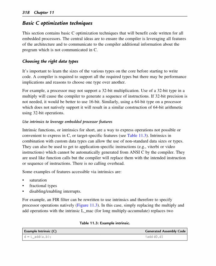
For example, an FIR filter can be rewritten to use intrinsics and therefore to specify

processor operations natively (Figure 11.3). In this case, simply replacing the multiply and

add operations with the intrinsic L_mac (for long multiply-accumulate) replaces two

Table 11.3: Example intrinsic.

Example Intrinsic (C) Generated Assembly Code

d 5 L_add(a,b); iadd d0,d1

318 Chapter 11

operations with one and adds the saturation function to ensure that DSP arithmetic is

handled properly.

Functions calling conventions

Each processor or platform will have different calling conventions. Some will be stack-

based, others register-based or a combination of both. Typically, default calling conventions

can be overridden though, which is useful. The calling convention should be changed for

functions unsuited to the default, such as those with many arguments. In these cases, the

calling conventions may be inefficient.

The advantages of changing a calling convention include the ability to pass more arguments

in registers rather than on the stack. For example, on some embedded processors, custom

calling conventions can be specified for any function through an application configuration

file and pragmas. It’s a two step process.

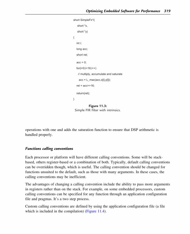
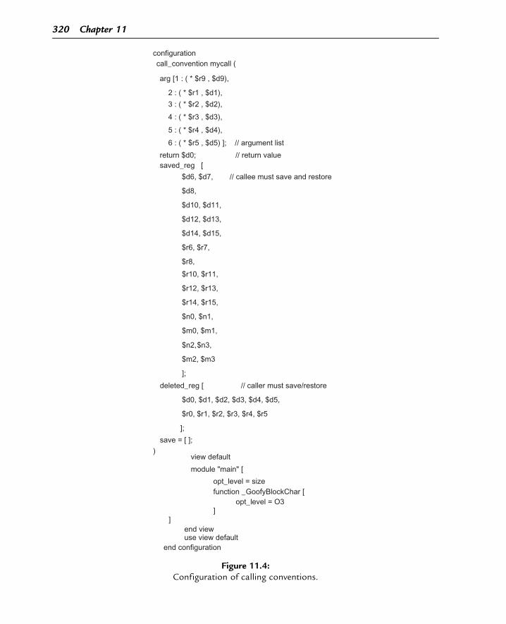
Custom calling conventions are defined by using the application configuration file (a file

which is included in the compilation) (Figure 11.4).

short SimpleFir1(

short *x,

short *y)

{

int i;

long acc;

short ret;

acc = 0;

for(i=0;i<16;i++)

// multiply, accumulate and saturate

acc = L_mac(acc,x[i],y[i]);

ret = acc>>16;

return(ret);

}

Figure 11.3:Simple FIR filter with intrinsics.


configurationcall_convention mycall (

arg [1 : ( * $r9 , $d9),

2 : ( * $r1 , $d1),

3 : ( * $r2 , $d2),

4 : ( * $r3 , $d3),

5 : ( * $r4 , $d4),

6 : ( * $r5 , $d5) ]; // argument list

return $d0; // return valuesaved_reg [

$d6, $d7, // callee must save and restore

$d8,

$d10, $d11,

$d12, $d13,

$d14, $d15,

$r6, $r7,

$r8,

$r10, $r11,

$r12, $r13,

$r14, $r15,

$n0, $n1,

$m0, $m1,

$n2, $n3,

$m2, $m3

];

deleted_reg [ // caller must save/restore

$d0, $d1, $d2, $d3, $d4, $d5,

$r0, $r1, $r2, $r3, $r4, $r5

];

save = [ ];)

view default

module "main" [

opt_level = sizefunction _GoofyBlockChar [

opt_level = O3]

]end viewuse view default

end configuration

Figure 11.4:Configuration of calling conventions.

320 Chapter 11

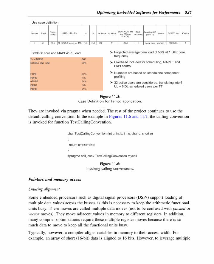
Use case definition

SC3850 core and MAPLW PE load

Sectors BandFrameconfig

ULUEs + DLUEs UL DL DL Mbps UL MbpsSR/ACK/CQI info

(per TTI overPUCCH)

RACHRoot seq

Sounding UE(per TTI) Device SC3850 freq. #Device

1 20 FDD 32+32 (6+6 sched per TTI) 1×2 2×2 102 51 1/32/1 1 1 wide band PSC9131 1000MHz 1

Projected average core load of 56% at 1 GHz corefrequency

Overhead included for scheduling, MAPLE andFAPI control

Numbers are based on standalone componentprofiling

32 active users are considered, translating into 6UL + 6 DL scheduled users per TTI

Total MCPS

SC3850 core load

FTPE

DEPE

PUPE

PDPE

eTVPE

563

56%

25%

5%

54%

5%

21%

Figure 11.5:Case Definition for Femto application.

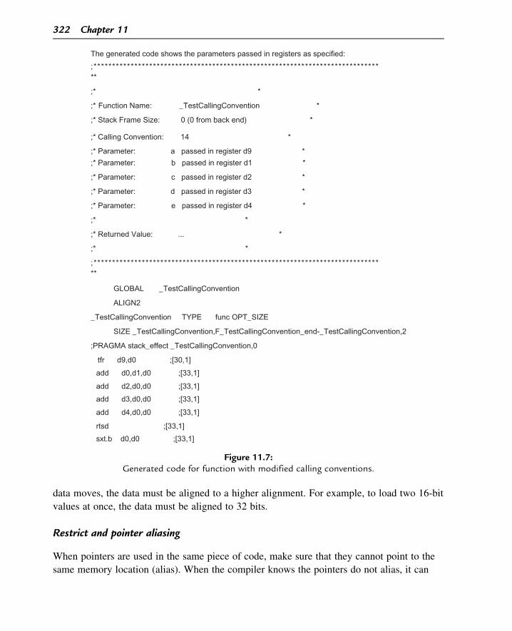
They are invoked via pragma when needed. The rest of the project continues to use the

default calling convention. In the example in Figures 11.6 and 11.7, the calling convention

is invoked for function TestCallingConvention.

Pointers and memory access

Ensuring alignment

Some embedded processors such as digital signal processors (DSPs) support loading of

multiple data values across the busses as this is necessary to keep the arithmetic functional

units busy. These moves are called multiple data moves (not to be confused with packed or

vector moves). They move adjacent values in memory to different registers. In addition,

many compiler optimizations require these multiple register moves because there is so

much data to move to keep all the functional units busy.

Typically, however, a compiler aligns variables in memory to their access width. For

example, an array of short (16-bit) data is aligned to 16 bits. However, to leverage multiple

char TestCallingConvention (int a, int b, int c, char d, short e)

{

return a+b+c+d+e;

}

#pragma call_conv TestCallingConvention mycall

Figure 11.6:Invoking calling conventions.


data moves, the data must be aligned to a higher alignment. For example, to load two 16-bit

values at once, the data must be aligned to 32 bits.

Restrict and pointer aliasing

When pointers are used in the same piece of code, make sure that they cannot point to the

same memory location (alias). When the compiler knows the pointers do not alias, it can

The generated code shows the parameters passed in registers as specified:

;*******************************************************************************

;* *

;* Function Name: _TestCallingConvention *

;* Stack Frame Size: 0 (0 from back end) *

;* Calling Convention: 14 *

;* Parameter: a passed in register d9 *

;* Parameter: b passed in register d1 *

;* Parameter: c passed in register d2 *

;* Parameter: d passed in register d3 *

;* Parameter: e passed in register d4 *

;* *

;* Returned Value: ... *

;* *

;*******************************************************************************

GLOBAL _TestCallingConvention

ALIGN2

_TestCallingConvention TYPE func OPT_SIZE

SIZE _TestCallingConvention,F_TestCallingConvention_end-_TestCallingConvention,2

;PRAGMA stack_effect _TestCallingConvention,0

tfr d9,d0 ;[30,1]

add d0,d1,d0 ;[33,1]

add d2,d0,d0 ;[33,1]

add d3,d0,d0 ;[33,1]

add d4,d0,d0 ;[33,1]

rtsd ;[33,1]

sxt.b d0,d0 ;[33,1]

Figure 11.7:Generated code for function with modified calling conventions.

322 Chapter 11

put accesses to memory pointed to by those pointers in parallel, greatly improving

performance. Otherwise, the compiler must assume that the pointers could alias.

Communicate this to the compiler by one of two methods: using the restrict keyword or by

informing the compiler that no pointers alias anywhere in the program (Figure 11.8).

The restrict keyword is a type qualifier that can be applied to pointers, references, and

arrays (Tables 11.4 and 11.5). Its use represents a guarantee by the programmer that within

the scope of the pointer declaration, the object pointed to can be accessed only by that

pointer. A violation of this guarantee can produce undefined results.

int *a;int *b;

a b

Figure 11.8:Illustration of pointer aliasing.

Table 11.4: Example loop before restrict added to parameters (DSP code).

Example Loop Generated Assembly Code

void foo (short * a,short * b,int N) {int i;for (i50;i,N;i11) {b[i]5shr(a[i],2);

}return;

}

doen3 d4FALIGNLOOPSTART3move.w (r0)1,d4asrr #,2,d4move.w d4,(r1)1

LOOPEND3

Table 11.5: Example loop after restrict added to parameters.

Example Loop with Restrict Qualifiers Added.

Note: Pointers a and b Must not Alias (ensure data is

located separately)

Generated Assembly Code.

Note: Now Accesses for a and b can be Issued

in Parallel

void foo (short * restrict a,short * restrict b,int N)

int i;for (i50;i,N;i11) {b[i]5shr(a[i],2);

}return;

}

move.w (r0)1,d4asrr #,2,d4doensh3 d2FALIGNLOOPSTART3

[ move.w d4,(r1)1 ; parallelmove.w (r0)1,d4 ; accesses

]asrr #,2,d4LOOPEND3move.w d4,(r1)


Loops

Communicating loop count information

Pragmas can be used to communicate to the compiler information about loop bounds to

help loop optimzation. If the loop minimum and maximum are known, for example, the

compiler may be able to make more aggressive optimizations.

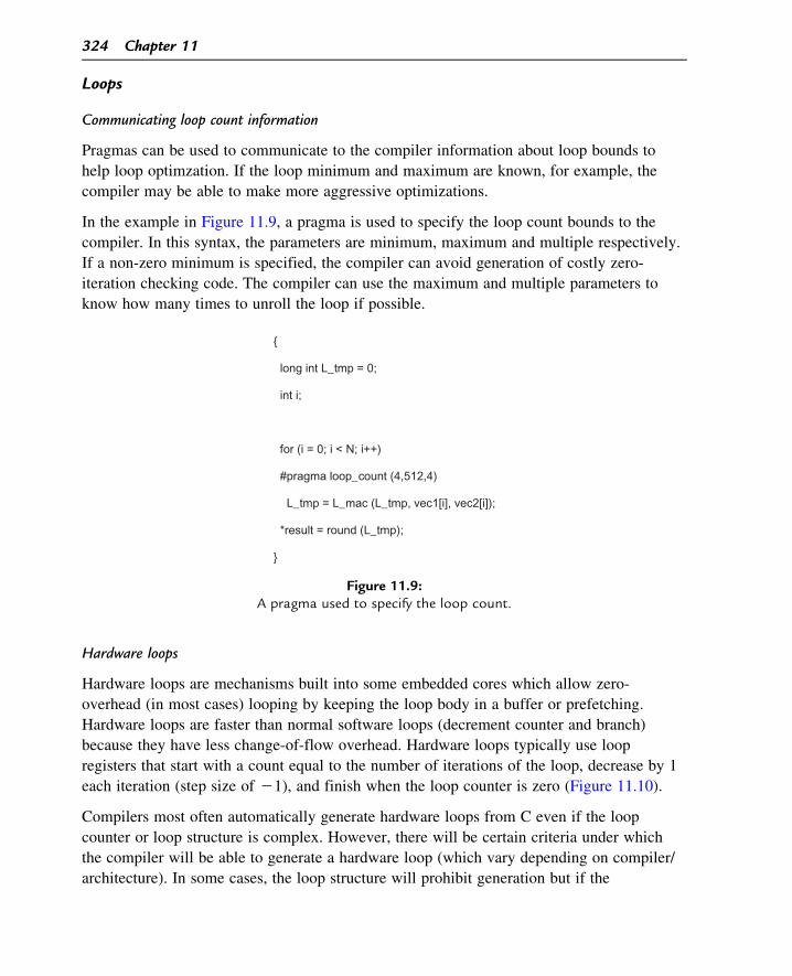
In the example in Figure 11.9, a pragma is used to specify the loop count bounds to the

compiler. In this syntax, the parameters are minimum, maximum and multiple respectively.

If a non-zero minimum is specified, the compiler can avoid generation of costly zero-

iteration checking code. The compiler can use the maximum and multiple parameters to

know how many times to unroll the loop if possible.

Hardware loops

Hardware loops are mechanisms built into some embedded cores which allow zero-

overhead (in most cases) looping by keeping the loop body in a buffer or prefetching.

Hardware loops are faster than normal software loops (decrement counter and branch)

because they have less change-of-flow overhead. Hardware loops typically use loop

registers that start with a count equal to the number of iterations of the loop, decrease by 1

each iteration (step size of 21), and finish when the loop counter is zero (Figure 11.10).

Compilers most often automatically generate hardware loops from C even if the loop

counter or loop structure is complex. However, there will be certain criteria under which

the compiler will be able to generate a hardware loop (which vary depending on compiler/

architecture). In some cases, the loop structure will prohibit generation but if the

{

long int L_tmp = 0;

int i;

for (i = 0; i < N; i++)

#pragma loop_count (4,512,4)

L_tmp = L_mac (L_tmp, vec1[i], vec2[i]);

*result = round (L_tmp);

}

Figure 11.9:A pragma used to specify the loop count.

324 Chapter 11

programmer knows about this, the source can be modified so the compiler can generate the

loop using hardware loop functionality. The compiler may have a feature to tell the

programmer if a hardware loop was not generated (compiler feedback). Alternatively, the

programmer should check the generated code to ensure hardware loops are being generated

for critical code.

As an example the StarCore DSP architecture supports four hardware loops. Note the

LOOPSTART and LOOPEND markings, which are assembler directives marking the start

and end of the loop body, respectively (Figure 11.11).

Figure 11.10:Hardware loop counting in embedded processors.

doensh3 #<5

move.w #<1,d0

LOOPSTART3

[ iadd d2,d1

iadd d0,d4

add #<2,d0

add #<2,d2 ]

LOOPEND3

Figure 11.11:StarCore DSP architecture.


Additional tips and tricks

The following are some additional tips and tricks to use for further code optimization.

Memory contention

When data is placed in memory, be aware of how the data is accessed. Depending on the

memory type, if two buses issue data transactions in a region/bank/etc., they could conflict

and cause a penalty. Data should be separated appropriately to avoid this contention. The

scenarios that cause contention are device-dependent because memory bank configuration

and interleaving differs from device to device.

Use of unaligned accesses

In some embedded processors, devices support unaligned memory access. This is

particularly useful for video applications. For example, a programmer might load four byte-

values which are offset by one byte from the beginning of an area in memory. Typically

there is a performance penalty for doing this.

Cache accesses

In the caches, place data that is used together next to each other in memory so that

prefetching the caches is more likely to obtain the data before it is accessed. In addition,

ensure that the loading of data for sequential iterations of the loop is in the same dimension

as the cache prefetch.

Inline small functions

The compiler normally inlines small functions, but the programmer can force inlining of

functions if for some reason it isn’t happening (for example if size optimization is

activated). For small functions the save, restore, and parameter-passing overhead can be

significant relative to the number of cycles of the function itself. Therefore, inlining is

beneficial. Also, inlining functions decreases the chance of an instruction cache miss

because the function is sequential to the former caller function and is likely to be

prefetched. Note that inlining functions increases the size of the code. On some processors,

pragma inline forces every call of the function to be inlined (Figure 11.12).

int foo () {

#pragma inline

...

}

Figure 11.12:Pragma inline forces.

326 Chapter 11

Use vendor run-time libraries

Embedded processor vendors typically provide optimized library functions for common run-

time routines like FFT, FIR, complex operations, etc. Normally, these are hand-written in

assembly as it still may be possible to improve performance over C. These can be invoked

by the programmer using the published API without the need to write such routines,

speeding time to market.

General loop transformations

The optimization techniques described in this section are general in nature. They are critical

to taking advantage of modern multi-ALU processors. A modern compiler will perform

many of these optimizations, perhaps simultaneously. In addition, they can be applied on all

platforms, at the C or assembly level. Therefore, throughout the section, examples are

presented in general terms, in C and in assembly.

Loop unrolling

Background

Loop unrolling is a technique whereby a loop body is duplicated one or more times. The

loop count is then reduced by the same factor to compensate. Loop unrolling can enable

other optimizations such as:

• multisampling

• partial summation

• software pipelining.

Once a loop is unrolled, flexibility in coding is increased. For example, each copy of the

original loop can be slightly changed. Different registers could be used in each copy. Moves

can be done earlier and multiple register moves can be used.

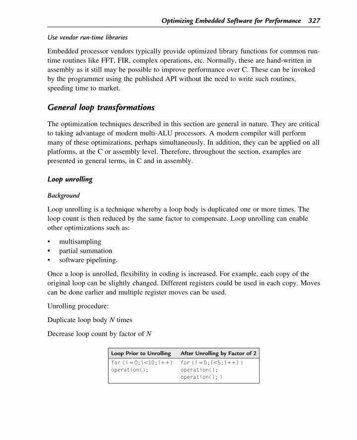
Unrolling procedure:

Duplicate loop body N times

Decrease loop count by factor of N

Loop Prior to Unrolling After Unrolling by Factor of 2

for (i50;i,10;i11) for (i50;i,5;i11) {operation(); operation();

operation(); }


Implementation

Figure 11.13 is an example of a correlation inner loop which as been unrolled by a factor

of two.

Multisampling

Background

Multisampling is a technique for maximizing the usage of multiple ALU execution units in

parallel for the calculation of independent output values that have an overlap in input

source data values. In a multisampling implementation, two or more output values are

calculated in parallel by leveraging the commonality of input source data values in

calculations. Unlike partial summation, multisampling is not susceptible to output value

errors from intermediate calculation steps.

Multisampling can be applied to any signal-processing calculation of the form:

y½n�5XM

m50

x½n1m�h½n�

where:

y[0]5 x[01 0]h[0]1 x[11 0]h[1]1 x[21 0]h[2]1 . . .1 x[M1 0]h[M]

y[1]5 x[01 1]h[0]1 x[11 1]h[1]1 . . .1 x[M2 11 1]h[M2 1]1 x[M1 1]h[M]

loopstart1

[ move.f (r0)+,d2 ; Load some data

move.f (r7)+,d4 ; Load some reference

mac d2,d4,d5 ; Do correlation

]

[ move.f (r0)+,d2 ; Load some data


mac d2,d4,d5 ; Do correlation

]

loopend1

Figure 11.13:A correlation inner loop.

328 Chapter 11

Thus, using C pseudocode, the inner loop for the output value calculation can be written as:

tmp1 5 x[n];for(m50; m,M; m1 52){tmp2 5 x[n1m11];y[n] 1 5 tmp1*h[m];y[n11] 1 5 tmp2*h[m];tmp1 5 x[k1m12];y[n] 1 5 tmp2*h[m11];y[n11] 1 5 tmp1*h[m11];}tmp2 5 x[n1m11];y[n11] 1 5 tmp2*h[m];

Implementation procedure

The multisampled version works on N output samples at once. Transforming the kernel into

a multisample version involves the following changes:

• changing the outer loop counters to reflect the multisampling by N

• use of N registers for accumulation of the output data

• unrolling the inner loop N times to allow for common data elements in the calculation

of the N samples to be shared

• reducing the inner loop counter by a factor of N to reflect the unrolling by N.

Implementation

An example implementation on a two-MAC DSP is shown in Figure 11.14.

Partial summation

Background

Partial summation is an optimization technique whereby the computation for one output

sum is divided into multiple smaller, or partial, sums. The partial sums are added together

at the end of the algorithm. Partial summation allows more use of parallelism since some

serial dependency is broken, allowing the operation to complete sooner.

Partial summation can be applied to any signal-processing calculation of the form:

y½n�5XM

m50

x½n1m�h½n�

where:

y[0]5 x[01 0]h[0]1 x[11 0]h[1]1 x[21 0]h[2]1 . . .1 x[M1 0]h[M]


To do a partial summation, each calculation is simply broken up into multiple sums. For

example, for the first output sample, assuming M5 3:

sum05 x[01 0]h[0]1 x[11 0]h[1]

sum15 x[21 0]h[0]1 x[31 0]h[1]

y[0]5 sum01 sum1

Note that the partial sums can be chosen as any part of the total calculation. In this example,

the two sums are chosen to be the first1 the second, and the third1 the fourth calculations.

Note: partial summation can cause saturation arithmetic errors. Saturation is not associative.

For example, saturate (a�b)1 c may not equal saturate (a�b1 c). Care must be taken to

ensure that such differences don’t affect the program.

[ clr d5 ; Clears d5 (accumulator)

clr d6 ; Clears d6 (accumulator)

move.f (r0)+,d2 ; Load data


]

move.f (r0)+,d3 ; Load data

InnerLoop:

loopstart1

[ mac d2,d4,d5 ; First output sample

mac d3,d4,d6 ; Second output sample

move.f (r0)+,d2 ; Load some data


]

[ mac d3,d4,d5 ; First output sample

mac d2,d4,d6 ; Second output sample

move.f (r0)+,d3 ; Load some data


]

loopend1

Figure 11.14:Partial summation.

330 Chapter 11

Implementation procedure

The partial summed implementation works on N partial sums at once. Transforming the

kernel involves the following changes:

• use of N registers for accumulation of the N partial sums;

• unrolling the inner loop will be necessary; the unrolling factor depends on the

implementation, how values are reused and how multiple register moves are used;

• changing the inner loop counter to reflect the unrolling.

Implementation

Figure 11.15 shows the implementation on a 2-MAC (multiply/accumulate) DSP.

Software pipelining

Background

Software pipelining is an optimization whereby a sequence of instructions is

transformed into a pipeline of several copies of that sequence. The sequences then

work in parallel to leverage more of the available parallelism of the architecture. The

sequence of instructions can be duplicated as many times as needed, substituting a

different set of registers for each sequence. Those sequences of instructions can then be

interwoven.

For a given sequence of dependent operations:

a5 operation();

b5 operation(a);

c5 operation(b);

Software pipelining gives (where operations on the same line can be parallelized):

a05 operation();

b05 operation(a); a15 operation();

c05 operation(b); b15 operation(a1);

c15 operation(b1);

Implementation

A simple sequence of three dependent instructions can easily be software pipelined, for

example the sequence in Figure 11.16. A software pipelining of three sequences is

shown. The sequence of code in the beginning where the pipeline is filling up (when

there are less than three instructions grouped) is the prologue. Similarly, the end

sequence of code with less than three instructions grouped is the epilogue. The grouping


[ move.4f (r0)+,d0:d1:d2:d3 ; Load data - x[..]

move.4f (r7)+,d4:d5:d6:d7 ; Load reference - h[..]]InnerLoop:

loopstart1[ mpy d0,d4,d8 ; x[0]*h[0]

mpy d2,d6,d9 ; x[2]*h[2]][ mac d1,d5,d8 ; x[1]*h[1]

mac d3,d7,d9 ; x[3]*h[3]move.f (r0)+,d0 ; load x[4]]add d8,d9,d9 ; y[0][ mpy d1,d4,d8 ; x[1]*h[0]

mpy d3,d6,d9 ; x[3]*h[1]moves.f d9,(r1)+ ; store y[0]][ mac d2,d5,d8 ; x[2]*h[2]

mac d0,d7,d9 ; x[4]*h[3]

move.f (r0)+,d1 ; load x[5]]add d8,d9,d9 ; y[1][ mpy d2,d4,d8 ; x[2]*h[0]mpy d0,d6,d9 ; x[4]*h{1]moves.f d9,(r1)+ ; store y[1]][ mac d3,d5,d8 ; x[3]*h[2]mac d1,d7,d9 ; x[5]*h[3]move.f (r0)+,d2 ;load x[6]]add d8,d9,d9 ; y[2][ mpy d2,d4,d8 ; x[3]*h[0]

mpy d0,d6,d9 ; x[5]*h[1]moves.f d9,(r1)+ ; store y[2]][ mac d3,d5,d8 ; x[4]*h[2]

mac d1,d7,d9 ; x[6]*h[3]move.f (r0)+,d3 load x[7]]add d8,d9,d9 ; y[3]moves.f d9,(r1)+ ; store y[3]loopend1

Figure 11.15:Software pipelined loop prolog.

332 Chapter 11

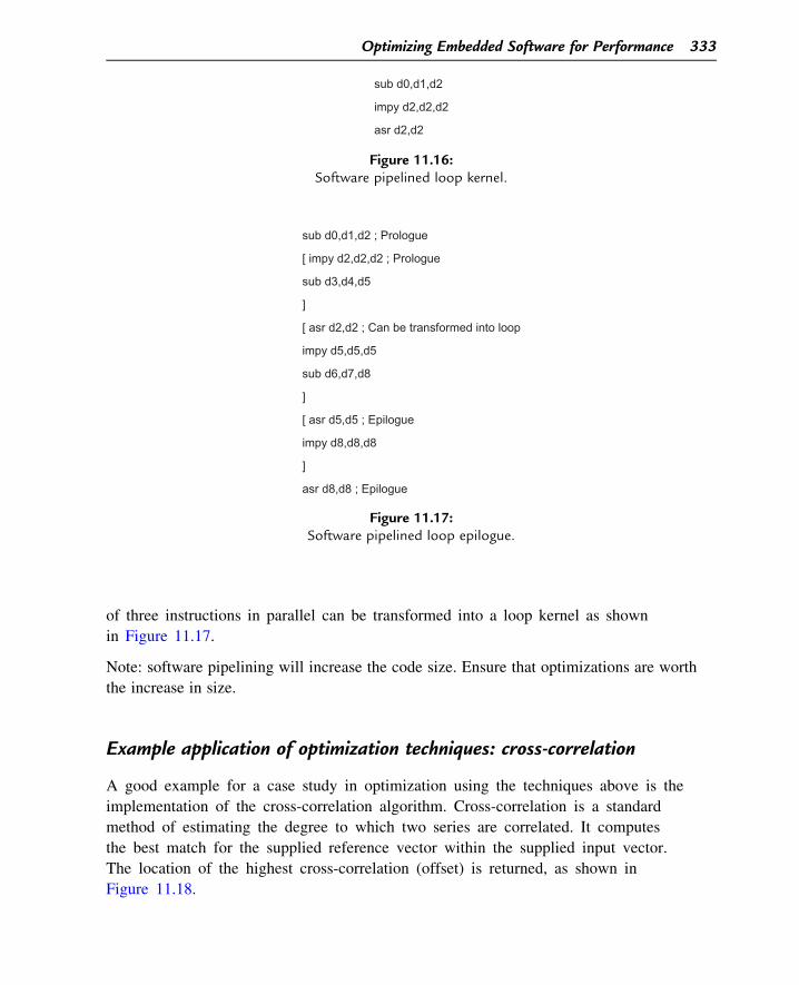
of three instructions in parallel can be transformed into a loop kernel as shown

in Figure 11.17.

Note: software pipelining will increase the code size. Ensure that optimizations are worth

the increase in size.

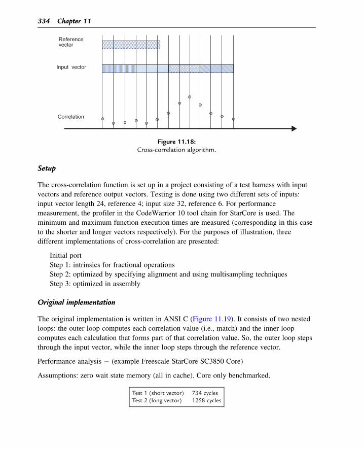
Example application of optimization techniques: cross-correlation

A good example for a case study in optimization using the techniques above is the

implementation of the cross-correlation algorithm. Cross-correlation is a standard

method of estimating the degree to which two series are correlated. It computes

the best match for the supplied reference vector within the supplied input vector.

The location of the highest cross-correlation (offset) is returned, as shown in

Figure 11.18.

sub d0,d1,d2

impy d2,d2,d2

asr d2,d2

Figure 11.16:Software pipelined loop kernel.

sub d0,d1,d2 ; Prologue

[ impy d2,d2,d2 ; Prologue

sub d3,d4,d5

]

[ asr d2,d2 ; Can be transformed into loop

impy d5,d5,d5

sub d6,d7,d8

]

[ asr d5,d5 ; Epilogue

impy d8,d8,d8

]

asr d8,d8 ; Epilogue

Figure 11.17:Software pipelined loop epilogue.


Setup

The cross-correlation function is set up in a project consisting of a test harness with input

vectors and reference output vectors. Testing is done using two different sets of inputs:

input vector length 24, reference 4; input size 32, reference 6. For performance

measurement, the profiler in the CodeWarrior 10 tool chain for StarCore is used. The

minimum and maximum function execution times are measured (corresponding in this case

to the shorter and longer vectors respectively). For the purposes of illustration, three

different implementations of cross-correlation are presented:

Initial port

Step 1: intrinsics for fractional operations

Step 2: optimized by specifying alignment and using multisampling techniques

Step 3: optimized in assembly

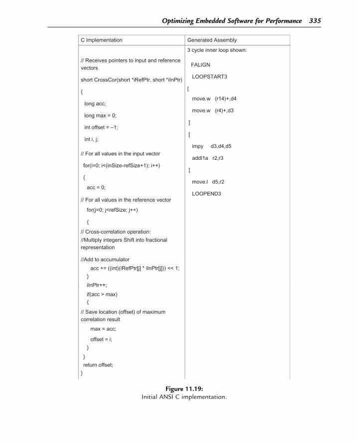
Original implementation

The original implementation is written in ANSI C (Figure 11.19). It consists of two nested

loops: the outer loop computes each correlation value (i.e., match) and the inner loop

computes each calculation that forms part of that correlation value. So, the outer loop steps

through the input vector, while the inner loop steps through the reference vector.

Performance analysis � (example Freescale StarCore SC3850 Core)

Assumptions: zero wait state memory (all in cache). Core only benchmarked.

Test 1 (short vector) 734 cyclesTest 2 (long vector) 1258 cycles

Referencevector

Input vector

Correlation

Figure 11.18:Cross-correlation algorithm.

334 Chapter 11

C Implementation Generated Assembly

// Receives pointers to input and reference vectors

short CrossCor(short *iRefPtr, short *iInPtr)

{

long acc;

long max = 0;

int offset = –1;

int i, j;

// For all values in the input vector

for(i=0; i<(inSize-refSize+1); i++)

{

acc = 0;

// For all values in the reference vector

for(j=0; j<refSize; j++)

{

// Cross-correlation operation:

//Multiply integers Shift into fractional representation

3 cycle inner loop shown:

FALIGN

LOOPSTART3

[

move.w (r14)+,d4

move.w (r4)+,d3

]

[

impy d3,d4,d5

addl1a r2,r3

]

move.l d5,r2

LOOPEND3

//Add to accumulator

acc += ((int)(iRefPtr[j] * iInPtr[j])) << 1;

}

iInPtr++;

if(acc > max){

// Save location (offset) of maximum correlation result

max = acc;

offset = i;

}

}

return offset;

}

Figure 11.19:Initial ANSI C implementation.


Step 1: use intrinsics for fractional operations and specify loop counts

In the first step, ensure that intrinsic functions are used to specify fractional operations to

ensure the best code is generated. On the Starcore SC3850 core, for example, there is a

multiply-accumulate instruction which does the left shift after the multiply and saturates

after the addition operation. This combines many operations into one. Replacing the inner

loop body with an L_mac intrinsic will ensure that the mac assembly instruction is

generated (Figure 11.20).




Step 2: specify data alignment and modify for multisampling algorithm

In the final step, multisampling techniques are used to transform the cross-correlation

algorithm. The cross-correlation code is modified so that two adjacent correlation

samples are calculated simultaneously. This allows data reuse between samples and a

reduction in data loaded from memory. In addition, aligning the vectors and using a

factor of two for multisampling ensures that when data is loaded, the alignment stays a

factor of two, which means multiple-register moves can be used, in this case, two values

at once (Figure 11.21). In summary, the changes are:

Multisampling: perform two correlation calculations each correlation per loop. Zero pad

first multiplication of second correlation (then compute the last multiply outside the

loop).

Reuse of data: since two adjacent correlation computations use some of the same

values, they can be reused, removing the need to refetch them from memory.

In addition, the one value reused between iterations is saved in a temporary

variable.

Since InSize-refSize1 1 correlations are needed and our vectors are even, there will be one

remaining correlation to calculate outside the loop (Figure 11.22).

Leveraging some assumptions made about the data set (even vectors), some more

aggressive optimizations could be done at the C level. This optimization means some

flexibility is given up for the sake of performance.


336 Chapter 11


long acc;

long max = 0;

int offset = -1;

int i, j;

for(i=0; i<inSize-refSize+1; i++) {

#pragma loop_count (24,32)

acc = 0;

for (j=0; j <= refSize+1; j++) {

#pragma loop_count (4,6)

acc = L_mac(acc, iRefPtr[j],

iInPtr[j]);

}

iInPtr++;

if(acc > max) {

max = acc;

One Inner Loop Only shown:

skipls ; note this was added due to

pragma loop count. Now if zero, skips loop

FALIGN

LOOPSTART3

DW17 TYPE debugsymbol

[

mac d0,d1,d2

move.f (r2)+,d1

move.f (r10)+,d0

]

LOOPEND3

offset = i;

}

}

return offset;

Figure 11.20:Intrinsic functions used to specify fractional operations to ensure the best code is generated.




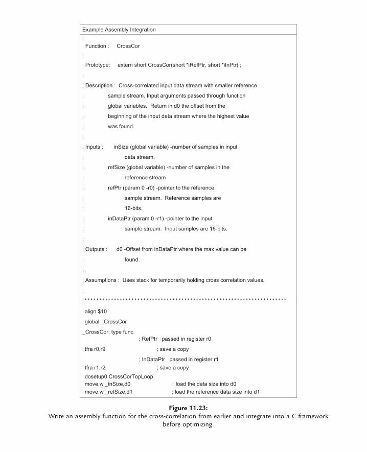
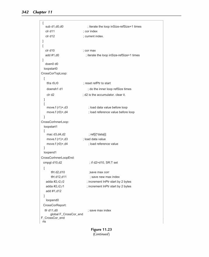
Step 3: assembly-language optimization

Assembly language is still used in cases where performance is critical. In this example

below, we will take the cross-correlation from earlier and write an assembly function,

integrate into a C framework then optimize it (Figure 11.23).




Seconditeration

Outsideinner loop

End of outerloop

corA =

corB =

i0 i1 i2 i3

i0 i1 i2 i3

r0 r1 r2 r3

0 r0 r1 r2

* * * * * * * *

* ** * * *

corA+=r0*i0corB+= 0*i0

corA+=r1*i1corB+=r0*i1



...

...

...

...

Reference; r(0)..r(n)Input; i(0)..i(m)Perform two correlations at once.Zero pad first multiplication of second correlationPerform two correlation calculations each correlation per loopReuse data each loop

i(n-1)

i(m-n) i(m)

N 0

One remaining cordue to zero padcorB+=r(n)*i(n-1)

r(0) r(n)

Insize-Refsize+1correlationsDo lastcorrelation

Figure 11.21:Diagram of multisampling technique.

338 Chapter 11


#pragma align *iRefPtr 4

#pragma align *iInPtr 4

long accA, accB;

long max = 0;

short s0,s1,s2,s3,s4;

int offset = -1;

int i, j;

for(i=0; i<inSize-refSize; i+=2) {


accA = 0;

accB = 0;

Both loop bodies shown:

skipls PL001

]FALIGN

LOOPSTART3 FALIGN LOOPSTART2

[tstgt d12 clr d8 clr d4 clr d5 suba r5,r5 move.l d13,r8

][

tfra r1,r2 s4 = 0;

for(j=0; j<refSize; j+=2) {


s0 = iInPtr[j];

s1 = iInPtr[j+1];

s2 = iRefPtr[j];

s3 = iRefPtr[j+1];

accA = L_mac(accA, s2, s0);

accB = L_mac(accB, s4, s0);

accA = L_mac(accA, s3, s1);


s4 = s3;

}

s0 = iInPtr[j];


jf L5 ]

[tfra r0,r3 addl1a r4,r2

][

move.2f (r2)+,d0:d1 move.2f (r3)+,d2:d3

][

mac d8,d0,d4 mac d2,d0,d8 tfr d3,d5 suba #<1,r8 tfra r9,r5

]doensh3 r8 FALIGN LOOPSTART3

Figure 11.22:Since InSize-ref Size1 1 correlations are needed and our vectors are even, there will be one

remaining correlation to calculate outside the loop.


if(accA > max) {

max = accA;

offset = i;

}

if(accB > max) {

max = accB;

offset = i+1;

}

iInPtr +=2;

}

accA = 0;

accB = 0;

for(j=0; j<refSize; j+=2) {


accA = L_mac(accA, iRefPtr[j],

iInPtr[j]);

accB = L_mac(accB,

[

mac d3,d1,d8 mac d2,d1,d4 move.2f (r2)+,d0:d1 ; packed

moves move.2f (r3)+,d2:d3

][

mac d2,d0,d8 mac d5,d0,d4 tfr d3,d5

]

LOOPEND3 [

mac d2,d1,d4 mac d3,d1,d8

][

cmpgt d9,d8 tfra r1,r2

iRefPtr[j+1], iInPtr[j+1]);

}

accA = L_add(accA, accB);

if(accA > max) {

max = accA;

offset = i;

}

return offset;

adda r4,r5 ][

tfrt d8,d9 tfrt d11,d10 addl1a r5,r2 adda #<2,r4

]move.f (r2),d1 mac d5,d1,d4 cmpgt d9,d4

[

IFT addnc.w #<1,d11,d10 IFA tfrt d4,d9 IFA add #<2,d11 ]

LOOPEND2

Figure 11.22(Continued)

340 Chapter 11

Example Assembly Integration

;; Function : CrossCor

;

; Prototype: extern short CrossCor(short *iRefPtr, short *iInPtr) ;

;

; Description : Cross-correlated input data stream with smaller reference

; sample stream. Input arguments passed through function

; global variables. Return in d0 the offset from the

; beginning of the input data stream where the highest value

; was found.

;

; Inputs : inSize (global variable) -number of samples in input

; data stream.

; refSize (global variable) -number of samples in the

; reference stream.

; refPtr (param 0 -r0) -pointer to the reference

; sample stream. Reference samples are

; 16-bits.

; inDataPtr (param 0 -r1) -pointer to the input

; sample stream. Input samples are 16-bits.

;

; Outputs : d0 -Offset from inDataPtr where the max value can be

; found.

;

; Assumptions : Uses stack for temporarily holding cross correlation values.

;

; * * * * * * * * * * * * * * * * * * * * * * * * * * * * * * * * * * * * * * * * * * * * * * * * * * * * * * * * * * * * * * * * * * * * *

align $10

global _CrossCor

_CrossCor: type func; RefPtr passed in register r0

tfra r0,r9 ; save a copy

; InDataPtr passed in register r1

tfra r1,r2 ; save a copy

dosetup0 CrossCorTopLoop move.w _inSize,d0 ; load the data size into d0move.w _refSize,d1 ; load the reference data size into d1

Figure 11.23:Write an assembly function for the cross-correlation from earlier and integrate into a C framework

before optimizing.

[sub d1,d0,d0 ; iterate the loop inSize-refSize+1 times

clr d11 ; cor index

clr d12 ; current index.

]

[

clr d10 ; cor max

add #1,d0 ; iterate the loop inSize-refSize+1 times

] doen0 d0

loopstart0

CrossCorTopLoop:

[

tfra r9,r0 ; reset refPtr to start

doensh1 d1 ; do the inner loop refSize times

clr d2 ; d2 is the accumulator. clear it.

][

move.f (r1)+,d3 ; load data value before loop

move.f (r0)+,d4 ; load reference value before loop

]

CrossCorInnerLoop:

loopstart1[

mac d3,d4,d2 ; ref[i]*data[i]

move.f (r1)+,d3 ; load data value

move.f (r0)+,d4 ; load reference value]

loopend1

CrossCorInnerLoopEnd:

cmpgt d10,d2 ; if d2>d10, SR:T set

[tfrt d2,d10 ;save max corr

tfrt d12,d11 ; save new max index

adda #2,r2,r2 ; increment InPtr start by 2 bytes

adda #2,r2,r1 ; increment InPtr start by 2 bytes

add #1,d12

]loopend0

CrossCorReport:

tfr d11,d0 ; save max indexglobal F_CrossCor_end

F_CrossCor_endrts

Figure 11.23(Continued)

342 Chapter 11

software engineering for embedded systems || optimizing embedded software for performance

Documents