socgen quant strategy - pricing bespoke cdos

World

Sector Report

28/07/2006

QUANTITATIVE STRATEGY Pricing bespoke CDOs: latest developments

Analysts Julien Turc (33) 1 42 13 40 90 [email protected]

David Benhamou (33) 1 42 13 94 76 [email protected]

Benjamin Herzog (33) 1 42 13 67 49 [email protected]

Marc Teyssier (33) 1 42 13 55 96 [email protected]

With contributions from Quantitative Research

Daniel Dahan

Laurent Prigneaux

Jerome Brun (Head)

Correlation Trading

Fouad Farah (Head)

Bespoke CDO pricing is one of the most complicated tasks for correlation desks and

CDO investors. Within the Gaussian copula framework, there are numerous ways to

account for bespoke portfolios and interpolate the base correlation surface.

We look at different ways to take into account non standard attachment points, non

standard maturities and bespoke portfolios. We show the pros and cons of each method

both from a theoretical and numerical point of view.

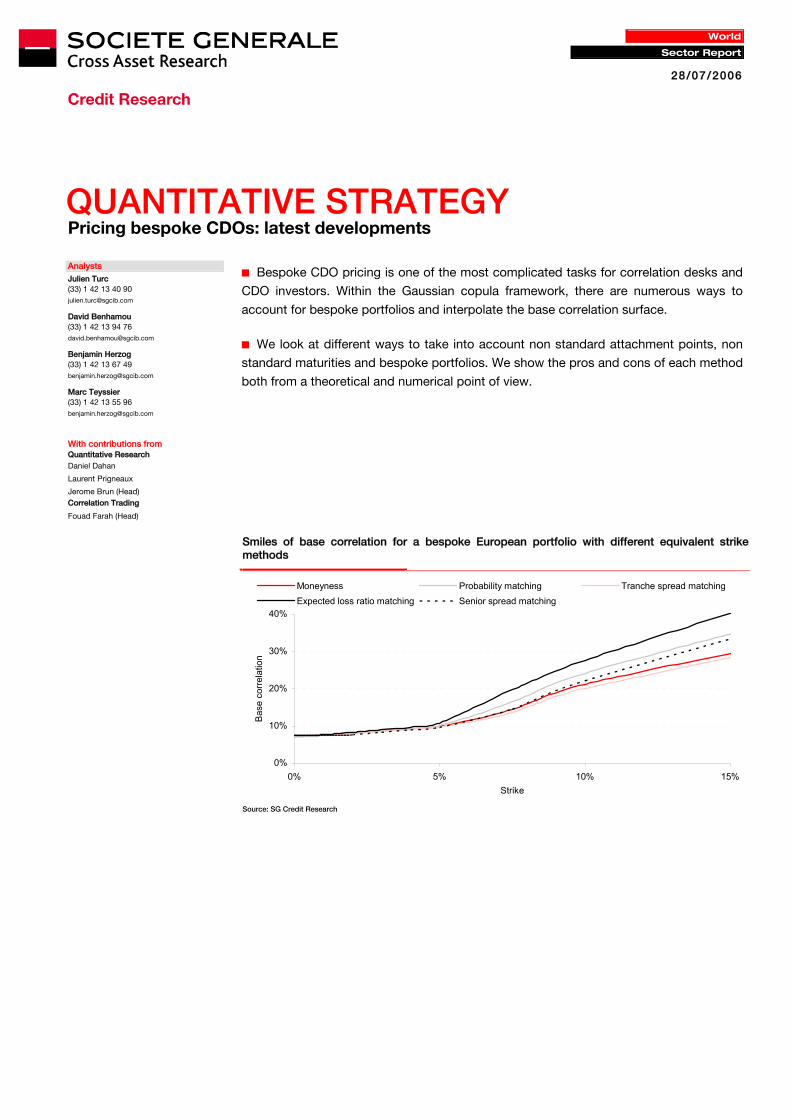
Smiles of base correlation for a bespoke European portfolio with different equivalent strike methods

0%

10%

20%

30%

40%

0% 5% 10% 15%Strike

Bas

e co

rrela

tion

Moneyness Probability matching Tranche spread matchingExpected loss ratio matching Senior spread matching

Source: SG Credit Research

Quantitative Strategy

28/07/2006 2

Contents

Generating the base correlation surface: how to price non-standard tranches on indices.............................................................4

Interpolating the base correlation smile across strikes for a given maturity..................4 Linear interpolation across strikes .....................................................................................4 Cubic spline interpolation across strikes ...........................................................................5 Outside the quoted range ..................................................................................................6

Interpolating the smile across maturities for a given strike .............................................7 Pricing American CDOs through zero-coupon CDOs........................................................7 Interpolating the American correlations across maturities.................................................8 Interpolating the zero-coupon correlations across maturities............................................8

Accounting for bespoke portfolios..................................................10

Bespoke portfolios with one reference index ..................................................................10 Moneyness matching.......................................................................................................10 Probability-matching........................................................................................................11 Equity spread matching ...................................................................................................13 Senior spread matching...................................................................................................13 Expected loss ratio matching ..........................................................................................14 Comparison of all equivalent strike methods...................................................................15

Bespoke portfolios with several reference indices .........................................................17 The separate weighted average method..........................................................................17 The joint weighted average method.................................................................................18 The beta method..............................................................................................................19


28/07/2006 3

For a given bespoke tranche, there are sometimes price differences across investment banks.

Indeed, there is no unique pricing framework across dealers. Even if the base correlation

Gaussian copula framework seems to remain the rule for most investment banks, the techniques

to account for bespoke portfolios are numerous and lead to significant price differences.

The purpose of this article is to analyse the pros and cons of several methods used in the

market for bespoke CDO pricing. This includes the methods to interpolate the base correlation

smile, to find the correlation assumptions for a bespoke tranche and to account for non

standard maturities. In the first part we discuss how to generate a base correlation surface

across maturities and strikes. In the second, we show how to account for bespoke portfolios,

i.e. how to determine the correlation assumptions used for a bespoke tranche.

All the methods presented in this report are based on the base correlation approach in the

Gaussian copula framework. This framework is detailed in our July 2004 article “Pricing and

Hedging correlation products”. Our local correlation model presented in our March 2005

article “Pricing CDO with a smile”, provides an alternative method for bespoke CDO pricing

and this will be discussed in a forthcoming article.


28/07/2006 4

Generating the base correlation surface: how to price non-standard tranches on indices

Before pricing bespoke CDO tranches, one needs to generate a base correlation surface for

each index (iTraxx, CDX, etc). This is a necessary step because bespoke CDO pricing requires

correlation assumptions that are taken from the standard index tranche market. Two issues

need to be addressed to generate the correlation surface of a given index:

How to interpolate the base correlation smile across strikes for a given maturity.

How to interpolate the base correlation smile across maturities for a given strike

Interpolating the base correlation smile across strikes for a given maturity The interpolation of the base correlation smile for a given maturity has a strong impact on the

pricing of non-standard tranches on indices and also on the pricing of bespoke tranches

based on these indices. We compare two methods for interpolating the smile (linear and cubic

spline interpolation) and discuss how to extrapolate the smile outside the quoted range.

Linear interpolation across strikes The first method consists in interpolating linearly between all quoted attachment points. For

example, one can interpolate linearly between the 3%, 6%, 9%, 12% and 22% base correlations

of the iTraxx index. The problem with the linear interpolation method is that it can generate

arbitrage opportunities since the slope of the base correlation smile is not continuous.

Indeed, the market-implied law of losses gives the probability for the loss to be below a given

strike, using the base correlation smile as an input (see our March 2005 article “Pricing CDOs

with a smile” for more details on this). According to the market-implied law of losses, the

probability for the portfolio loss to be below K is:

( ) ( , ) ( , )* ( , )K K KP Loss K P Loss K Skew K Rho Kρ ρ ρ< = < −

where ( , )KP Loss K ρ< is the probability for the loss to be below K using the naive

cumulative loss function for the [0-K] tranche with the base correlation Kρ for strike K,

( , )KSkew K ρ is the slope (or skew) of the base correlation smile for strike K and

where ( , )KRho K ρ is the derivative of the expected loss of the [0-K] tranche with respect to

the correlation ρ. This formula shows that if the skew of the base correlation smile is

discontinuous when K increases, the probability for the loss to be below K can be discontinuous.

For example, if the slope jumps downwards between K and K+ε, the probability for the loss to

be below K+ε may be lower than the probability for the loss to be below K which leads to

negative probabilities for the loss to be between K and K+ε. Even if the slope of the smile is

continuous, P(Loss<K) may decrease between two strikes K1< K2 if the slope of the smile

changes abruptly between K1and K2. This also generates arbitrages between tranches.

Linear interpolation across strikes is the simplest method but it generates arbitrages on tiny tranches


28/07/2006 5

For example, a 10y 8.9%-9% tranche on the iTraxx S5 index was priced at 68bp on 6 June

2006 with a linear interpolation of the base correlation smile while a 9%-9.1% was priced at

84bp. This is an arbitrage opportunity since it is possible to sell protection on the 9%-9.1%

tranche, buy protection on the 8.9%-9% tranche and lock a +16bp positive carry without any

risk. These arbitrages are difficult to execute in practice because it is hard to enter such thin

tranches. Nevertheless, these arbitrage opportunities are dangerous when pricing squared

CDOs or bespoke CDOs. Our February 2006 article �CDO²: new opportunities” details a

technique for CDO² pricing. It shows that computing portfolio loss distribution is key to

determining CDO² spreads. Jumps in the slope of the correlation smile lead to inconsistent

loss distributions and therefore to arbitrages in CDO² prices. In some equivalent strike

methods, inconsistent loss distribution also lead to arbitrage in bespoke CDO pricing, for

example bespoke tranches with negative spreads. As a result, we favour interpolation

methods that are more continuous than the linear interpolation method.

Cubic spline interpolation across strikes The cubic spline interpolation method consists in fitting second-order polynomial functions on

each part of the base correlation smile so as to obtain a curve that is continuous and whose

slope is continuous. Since the slope of the base correlation smile is continuous, this method

generates portfolio loss distributions that are consistent most of the time, i.e. the probability

for the loss to be in any given range is always positive. Nevertheless, some arbitrage

opportunities may exist even with a cubic spline interpolation if the convexity of the base

correlation smile changes too abruptly. For example, a 10y 8.9%-9% tranche on the iTraxx S5

index was priced at 65bp on 6 June 2006 with a cubic spline interpolation of the base

correlation smile while a 9%-9.1% was priced at 68bp. This example shows that there is a

small arbitrage opportunity between the 8.9-9% and 9-9.1% tranches (3bp carry for a risk-free

position) but that this arbitrage is �smaller� than the arbitrage with the linear interpolation

method (16bp for a risk-free position).

Cubic spline interpolation is better than linear interpolation but some arbitrage opportunities may still exist with this method


28/07/2006 6

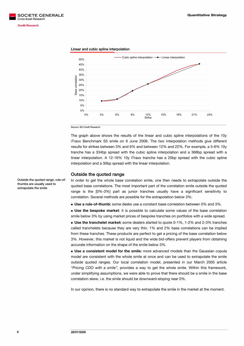
Linear and cubic spline interpolation

0%

5%

10%

15%

20%

25%

30%

35%

40%

45%

50%

0% 3% 6% 9% 12% 15% 18% 21% 24%Strike

Bas

e co

rrela

tion

Cubic spline interpolation Linear interpolation


The graph above shows the results of the linear and cubic spline interpolations of the 10y

iTraxx Benchmark S5 smile on 6 June 2006. The two interpolation methods give different

results for strikes between 3% and 6% and between 12% and 22%. For example, a 5-6% 10y

tranche has a 334bp spread with the cubic spline interpolation and a 368bp spread with a

linear interpolation. A 12-16% 10y iTraxx tranche has a 20bp spread with the cubic spline

interpolation and a 30bp spread with the linear interpolation.

Outside the quoted range In order to get the whole base correlation smile, one then needs to extrapolate outside the

quoted base correlations. The most important part of the correlation smile outside the quoted

range is the [0%-3%] part as junior tranches usually have a significant sensitivity to

correlation. Several methods are possible for the extrapolation below 3%:

Use a rule-of-thumb: some desks use a constant base correlation between 0% and 3%.

Use the bespoke market: it is possible to calculate some values of the base correlation

smile below 3% by using market prices of bespoke tranches on portfolios with a wide spread.

Use the tranchelet market: some dealers started to quote 0-1%, 1-2% and 2-3% tranches

called tranchelets because they are very thin. 1% and 2% base correlations can be implied

from these tranches. These products are perfect to get a pricing of the base correlation below

3%. However, this market is not liquid and the wide bid-offers prevent players from obtaining

accurate information on the shape of the smile below 3%.

Use a consistent model for the smile: more advanced models than the Gaussian copula

model are consistent with the whole smile at once and can be used to extrapolate the smile

outside quoted ranges. Our local correlation model, presented in our March 2005 article

“Pricing CDO with a smile”, provides a way to get the whole smile. Within this framework,

under simplifying assumptions, we were able to prove that there should be a smile in the base

correlation skew, i.e. the smile should be downward-sloping near 0%.

In our opinion, there is no standard way to extrapolate the smile in the market at the moment.

Outside the quoted range, rule-of-thumbs are usually used to extrapolate the smile


28/07/2006 7

Interpolating the smile across maturities for a given strike Pricing CDOs with non standard maturities, i.e. maturities other than 5y, 7y and 10y, requires

interpolating the smile across maturities. This interpolation can be addressed through several

techniques. We detail two possible methods here:

Interpolating the American correlations across maturities. This involves a linear interpolation

between quoted flat American correlations.

Building the zero-coupon correlations across maturities. This requires a bootstrapping of the

zero-coupon correlation term structure to fit to market prices of index tranches.

A zero-coupon CDO is a CDO for which all protection payments are paid at the end and there

is no spread payment over the life of the product. This convention is not used in practice

except for zero-coupon equity pieces. The market convention for bespoke CDOs and index

tranches is to use American CDOs, for which protection payments are made as soon as a

default occurs and for which spread payments are proportional to the remaining notional in

the tranche. The first method detailed here solely considers American CDOs while the second

method uses zero-coupon CDOs as building blocks to interpolate the smile across maturities.

Before detailing several techniques for the interpolation across maturities, we first recap the

process required for pricing American CDOs through the pricing of zero-coupon CDOs.

Pricing American CDOs through zero-coupon CDOs The most standard algorithm to price CDOs is the recursive algorithm which enables to find the

expected loss of the [0-K] tranche for a given time horizon T. The algorithm uses three inputs:

spread curves, recovery rates for each name and a correlation assumption. It is much faster than

Monte-Carlo simulations but does not provide the timing of defaults: it solely gives the loss

distribution at a given maturity T but not before. Nevertheless, it can be used to price American

CDO tranches that require knowing the expected loss of the tranche at all times. Pricing a [0-K]

American tranche requires pricing the protection leg and the fee leg of the tranche:

The protection leg of the tranche writes:

( )0 0( ) , ( )t

T r tUS ZCt ZCExpLoss T e dExpLoss t tρ−= ∫ (1)

( )0 0 00( ) ( , ( )) , ( )

TUS ZC ZCZC t ZCExpLoss T ExpLoss T t r ExpLoss t t dtρ ρ= + ∫ (2)

where ( ), ( )ZCt ZCExpLoss τ ρ τ is the expected loss in the zero-coupon tranche at time τ

discounted at time t and ( )ZCρ τ is the zero-coupon correlation with maturity τ.

The fee leg of the tranche writes:

( ) 1* 01 * 1 , ( ) ( )t ii

i

r t ZCt i ZC i i i

iSpread DV Spread e ExpLoss t t t tρ−

−⎡ ⎤= − −⎣ ⎦∑

where the times ti are the fee payment times.

These two formulas show how to price an American CDO through several zero-coupon CDO

pricings.

We show how to interpolate the American and zero-coupon correlation term curve

Standard algorithms rely on zero-coupon CDO pricing. American CDOs can be priced through zero-coupon CDO pricing


28/07/2006 8

Interpolating the American correlations across maturities This method consists in two different steps:

Compute the flat base correlations that give the right prices for the quoted tranches

(5y, 7y and 10y). Since these tranches are American, the base correlations are American.

Interpolate between these correlations, for example linearly, to obtain American base

correlations for all maturities.

For example a 6y 0-6% tranche is then priced with one American base correlation which is the

average of the 5y 0-6% base correlation and the 7y 0-6% base correlation.

This method is computationally efficient and easy to implement. Its main drawback is that it only

gives American base correlations. Therefore, any pricing that requires zero-coupon base

correlation is difficult, for example for CDO², tranche options, zero-coupon equity, etc. It is

nevertheless possible to imply zero-coupon base correlations from American base correlations.

Interpolating the zero-coupon correlations across maturities The second method requires constructing a term structure for zero-coupon correlation. As

shown above, an American CDO is equivalent to a portfolio of zero-coupon CDOs expiring at

successive maturities (for example every three months). There are two ways to price an

American CDO with the recursive algorithm:

Use a flat base correlation (called the American correlation) to price all the zero-coupon

CDOs that constitute the American CDO.

Price each zero-coupon CDO with its zero-coupon base correlation, assuming a zero-

coupon correlation term curve.

The second method requires specifying a shape for the zero-coupon correlation term

structure. Among possible shapes, piecewise-constant or piecewise-linear curves are the

easiest to implement. Once this shape has been set (for example a piecewise-linear term

curve), it is possible to bootstrap each part of the correlation term structure from the quoted

market prices of American tranches.

Let us consider the example of the 3% zero-coupon correlation term structure. Using the market

price for the 5y 0-3% tranche, one can find the zero-coupon correlation that is consistent with

this price, assuming a constant zero-coupon correlation between 0 and 5 years. Then, using the

market price for the 7y 0-3% tranche, one can find the 7y zero-coupon correlation that is

consistent with this price, assuming a linear zero-coupon correlation term curve between 5y and

7y. Lastly, the 10y 0-3% tranche gives the value of the 10y zero-coupon correlation.


28/07/2006 9

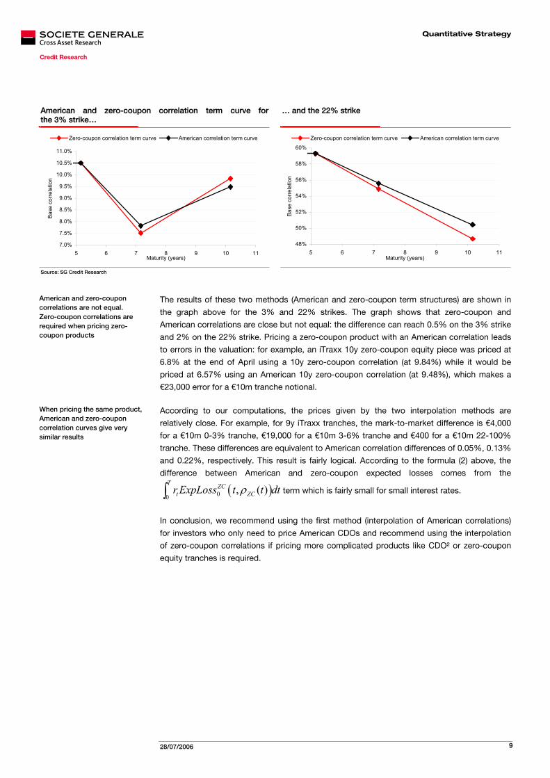
American and zero-coupon correlation term curve for the 3% strike…

… and the 22% strike

7.0%

7.5%

8.0%

8.5%

9.0%

9.5%

10.0%

10.5%

11.0%

5 6 7 8 9 10 11Maturity (years)

Base

cor

rela

tion

Zero-coupon correlation term curve American correlation term curve

48%

50%

52%

54%

56%

58%

60%

5 6 7 8 9 10 11Maturity (years)

Base

cor

rela

tion

Zero-coupon correlation term curve American correlation term curve


The results of these two methods (American and zero-coupon term structures) are shown in

the graph above for the 3% and 22% strikes. The graph shows that zero-coupon and

American correlations are close but not equal: the difference can reach 0.5% on the 3% strike

and 2% on the 22% strike. Pricing a zero-coupon product with an American correlation leads

to errors in the valuation: for example, an iTraxx 10y zero-coupon equity piece was priced at

6.8% at the end of April using a 10y zero-coupon correlation (at 9.84%) while it would be

priced at 6.57% using an American 10y zero-coupon correlation (at 9.48%), which makes a

�23,000 error for a �10m tranche notional.

According to our computations, the prices given by the two interpolation methods are

relatively close. For example, for 9y iTraxx tranches, the mark-to-market difference is �4,000

for a �10m 0-3% tranche, �19,000 for a �10m 3-6% tranche and �400 for a �10m 22-100%

tranche. These differences are equivalent to American correlation differences of 0.05%, 0.13%

and 0.22%, respectively. This result is fairly logical. According to the formula (2) above, the

difference between American and zero-coupon expected losses comes from the

( )00, ( )

T ZCt ZCr ExpLoss t t dtρ∫ term which is fairly small for small interest rates.

In conclusion, we recommend using the first method (interpolation of American correlations)

for investors who only need to price American CDOs and recommend using the interpolation

of zero-coupon correlations if pricing more complicated products like CDO² or zero-coupon

equity tranches is required.

American and zero-coupon correlations are not equal. Zero-coupon correlations are required when pricing zero-coupon products

When pricing the same product, American and zero-coupon correlation curves give very similar results


28/07/2006 10

Accounting for bespoke portfolios

Finding the right correlation assumption for a bespoke portfolio is a tricky task. We start by

showing solutions for this problem when the bespoke portfolio has only one reference tranche

market (iTraxx tranches, for example). Portfolios that mix European and US names are

analysed in the second part of this section.

Bespoke portfolios with one reference index Pricing bespoke tranches requires finding their equivalent index tranches. Once this equivalent

tranche has been determined, pricing the bespoke tranche is easy. It simply consists in

applying the standard Gaussian copula pricer to the bespoke portfolio with the base

correlations of the equivalent index tranche. Since the equivalent index tranche is not

necessarily a standard index tranche (for example, it could be a 6y 4%-5.2% iTraxx tranche),

finding the base correlations of this equivalent tranche requires having a base correlation

surface for each index. This issue was addressed in the prior section.

Pricing a [K1-K2] tranche with the base correlation approach requires pricing the two equity

tranches [0-K1] and [0-K2]. We describe here five possible methods to find the equivalent

index tranche [0-Kindex] for a bespoke equity tranche [0-Kbespoke]:

Moneyness matching: the bespoke and index equivalent tranches have the same

�moneyness� defined as the ratio between the attachment point and the expected loss of the

portfolio. For example, a [0-8%] bespoke tranche is equivalent to a [0-4%] index tranche if the

bespoke portfolio expected loss is twice as wide as the index expected loss.

Probability matching: the bespoke and index equivalent tranches have the same probability

to get wiped out.

Equity spread matching: the bespoke and index equivalent equity tranches [0-K] have the

same spread.

Senior spread matching: the bespoke and index equivalent senior tranches

[K-100] have the same spread.

Expected loss ratio matching: the expected loss of the two equivalent equity tranches

represents the same percentage of the expected loss of their respective portfolios.

Moneyness matching The moneyness matching approach consists in finding the equivalent tranche that has the

same �moneyness� as the bespoke tranche. The moneyness is defined as the ratio between

the attachment point and the portfolio�s expected loss. Therefore, the method consists in

finding Kindex that verifies:

index bespoke

index portfolio bespoke portfolio

K KExpLoss ExpLoss

=

One alternative and fairly equivalent way to compute the moneyness is to compute the ratio

between the strike and the portfolio spread. The spread of the portfolio can be interpreted as

the average expected loss per year. Therefore, having the same moneyness for two tranches

can be interpreted as having the same expected time to get wiped out.

Five equivalent strike methods are analysed in this paper

The moneyness approach matches the ratio of the strike and the portfolio’s expected loss for the bespoke and index tranche


28/07/2006 11

The main advantage of this method is that it is very easy to implement and is immediate. It

nevertheless has three major drawbacks:

If the bespoke portfolio spread is very tight compared to the index spread, the equivalent

attachment point is very high in the capital structure and may be more senior than most senior

quoted tranches. Let us consider the example of a European bespoke tranche with 100 names

trading at 15bp. Any tranche senior to 10.5% has an equivalent attachment point that is higher

than 22% in Europe, and its correlation assumption is therefore rather arbitrary.

More importantly, the moneyness approach does not take into account the dispersion of the

bespoke portfolio but only its expected loss. Therefore, it does not distinguish between a

45bp homogeneous portfolio (all CDS trading at 45bp) and a portfolio with all names trading

tighter (say at 30bp) except one CDS trading close to default (say at 10000bp). This is a

problem for equity tranches because in the first case (homogeneous portfolio), an equity

tranche is not very risky while in the second case it is extremely risky.

The P&L of a bespoke tranche is discontinuous in case of default using the moneyness

approach. When a default occurs in the bespoke or index portfolio, the ratio of expected

losses of the bespoke and index portfolio changes suddenly. As a result, the equivalent strike

and equivalent correlation change, and this creates a discontinuity in the P&L of the tranche.

Let us take the example of a �10m [0-4%] tranche on a portfolio of 99 names trading at 30bp

and one name trading at 50,000bp. The equivalent strike of this tranche is 3.1% and its

correlation is 10.3%. If the risky name defaults and the recovery rate is 40%, the protection

buyer receives 0.6% of the overall portfolio notional, which represents �1.5m (15% of the

tranche notional). Therefore, the tranche becomes a [0-3.4%] tranche on a portfolio of 99

names at 30bp. The new equivalent strike of this tranche is 3.65% which has a correlation of

12.4%. The mark-to-market of the long protection position in the tranche decreases by

�1.575m after the default, and therefore the default generates a negative P&L of -�75,000

(+�1.5m-�1.575m=-�75,000) for the protection buyer. The discontinuity in case of default is a

very significant drawback of this method.

Probability-matching For the probability matching approach, the equivalent tranche is the index tranche that has the

same probability of being eliminated as the bespoke tranche. This writes:

( ) ( ), ,bespoke bespoke index index index indexP Loss K P Loss Kρ ρ≤ = ≤

This method is not completely straightforward as computing the probability of elimination of a

bespoke tranche requires a correlation assumption which itself depends on the equivalent strike.

This method works well when taking into account the portfolio dispersion. It is also continuous

in case of default. For example, the P&L of a long �10m [0-4%] tranche on a portfolio of 99

names at 30bp and one name at 50,000bp moves only by �3,000 in case of default of the

risky name, and the equivalent strikes of the pre-default and post-default tranches are very

close (5.12% and 5.08%).

The moneyness approach is easy to implement but it does not take dispersion into account and is discontinuous in case of default

The probability-matching approach takes dispersion into account and is continuous in case of default

The probability-matching method matches the probabilities for the bespoke and index strikes to get hit


28/07/2006 12

On the other hand, this method has two drawbacks:

Computing equivalent strikes is numerically difficult when using deterministic recovery rates.

Because of this assumption, the loss distribution function is not continuous and subtle

numerical schemes are required to create a continuous loss distribution. For example, if all

names have a recovery rate of 40% and there are 100 names in the portfolio, the possible

losses are multiples of 0.6%. As a result, the loss distribution function is piecewise-constant

with discontinuities for each multiple of 0.6%. Furthermore, even with a continuous loss

distribution function this method is quite time consuming.

The probability matching method does not work well for bespoke portfolios with a wide spread.

Let�s look at a 5y portfolio with 100 names all trading at 100bp. For the benchmark S5 index, the

probability for the loss to be zero after five years was 14%, according to our calculations on

6 June 2006. On the other hand, for any correlation assumption, the probability that bespoke

strikes below 1.3% are not hit is lower than 14% because of the wide spread of the bespoke

portfolio. As a result, there isn�t any equivalent strike for bespoke strikes lower than 1.3%.

In this case, one solution is to take the 0% base correlation as the correlation assumption for

these bespoke tranches. Nevertheless, this example shows that the Main index is not the right

reference for wide portfolios and that High Yield index tranches, at least in the US, may be

more appropriate.

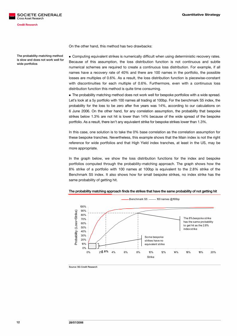
In the graph below, we show the loss distribution functions for the index and bespoke

portfolios computed through the probability-matching approach. The graph shows how the

8% strike of a portfolio with 100 names at 100bp is equivalent to the 2.8% strike of the

Benchmark S5 index. It also shows how for small bespoke strikes, no index strike has the

same probability of getting hit.

The probability matching approach finds the strikes that have the same probability of not getting hit

0%10%20%30%40%50%60%70%80%90%

100%

0% 2% 4% 6% 8% 10% 12% 14% 16% 18% 20%

Strike

Prob

abilit

y (L

oss<

Strik

e)

Benchmark S5 100 names @100bp

2.8%

The 8% bespoke strike has the same probability to get hit as the 2.8% index strike

Some bespoke strikes have no equivalent strike


The probability-matching method is slow and does not work well for wide portfolios


28/07/2006 13

Equity spread matching The equity spread matching methodology consists in finding the equivalent index equity

tranche [0-Kindex] that has the same spread as the bespoke equity tranche [0-Kbespoke]. A

correlation assumption is needed to compute the bespoke tranche spread and this correlation

assumption itself depends on the equivalent tranche. Therefore, as is the case with the

probability-matching approach, a numerical solving is also required.

This method takes dispersion into account. It nevertheless has three major drawbacks:

It does not work very well when the bespoke portfolio spread is tight. In this case, for senior

tranches, the tranche spread is quite tight too and generates an equivalent strike higher than

most senior quoted tranches. For example, for a European bespoke portfolio of 100 names

trading at 15bp, any strike higher than 8.6% has an equivalent strike higher than 22%. If the

tranche is too senior, there may be no equivalent tranche at all. Indeed, if the bespoke tranche

spread is below the index portfolio spread (which is the spread of the tranche [0-100%]), then

no index tranche matches the spread of the bespoke tranche. This case is rare though: for a

European portfolio of 100 names trading at 15bp, this happens only for strikes higher than

47% which are unlikely to be useful in practice.

It does not work well for junior tranches on bespoke portfolios with wide spreads. There is a

maximum possible spread for an index tranche. For example, a [0%-0.01%] tranche on the iTraxx

S5 index was priced at 3210bp on 6 June 2006. If the bespoke tranche is too risky, there may not

be any index equivalent tranche with the same spread. For example, for a bespoke portfolio with

100 names trading at 100bp, any strike lower than 2.7% does not have any equivalent strike.

It is not continuous in case of default, for example for a bespoke [0-4%] tranche on a

portfolio with 99 names at 30bp and one name at 50,000bp. In case of default, the equivalent

strike changes from 2.9% to 3.8% due to the default of the risky name and this generates a

-�65,000 P&L for a long �10m protection position.

Senior spread matching An alternative way to implement a spread matching approach is to match senior tranche

spreads instead of equity tranche spreads. Therefore, it involves finding the index tranche

[Kindex -100%] that has the same spread as the bespoke tranche [Kbespoke-100%]. This method

is not equivalent to the equity tranche spread matching.

For tight bespoke portfolios, the senior spread matching approach works better than the equity

spread matching approach. For example for a European portfolio with 100 names trading at 15bp,

any tranche lower than 12.75% had an equivalent strike lower than 22% on 6 June 2006.

For wide bespoke portfolios, the senior spread matching approach is worse than the equity

spread matching approach because it does not find any equivalent strike for a wide range of

tranches. In fact, the spread of a [K-100%] tranche on the index is capped by the index

spread (which is the spread of a [0%-100%] tranche). Therefore, if the bespoke spread is

wide, some tranches [K-100%] have a spread that is higher than the index spread for any

possible correlation assumption and in this case, there is no equivalent strike. For example, for

a European portfolio with 100 names at 100bp, any strike lower than 4.9% did not have any

equivalent strike on 6 June 2006 with the senior spread matching methodology.

It is almost continuous in case of default. The spread of the senior tranches is less sensitive

to default. Therefore this method is far more robust in case of default. Let us take the example

of a European bespoke [0-4%] tranche on a portfolio with 99 names at 30bp and one name at

50,000bp. In case of default of the risky name, the equivalent strike changes from 3.44% to

3.36% due to the default of the risky name and this generates a +�5,000 P&L for a long �10m

protection position.

The equity spread matching takes dispersion into account.

The senior spread matching approach matches the spread of the senior bespoke and index tranches [K-100]

It works well for tight portfolios but does not work for most wide portfolios

It is almost continuous in case of default

It does not work well for tight and wide portfolios

It is discontinuous in case of default

This method matches the spread of the bespoke and index equity tranches [0-K]


28/07/2006 14

Expected loss ratio matching The last method we present here is relatively similar to the moneyness approach. Two

tranches are equivalent if they have the same moneyness, defined as the ratio between the

expected loss of the equity tranche and the expected loss of the portfolio. Therefore the

bespoke tranche Kbespoke and the equivalent tranche Kindex verify:

0 0index index bespoke bespoke

index portfolio bespoke portfolio

ExpLoss K ExpLoss KExpLoss ExpLoss

⎡ ⎤ ⎡ ⎤− −⎣ ⎦ ⎣ ⎦=

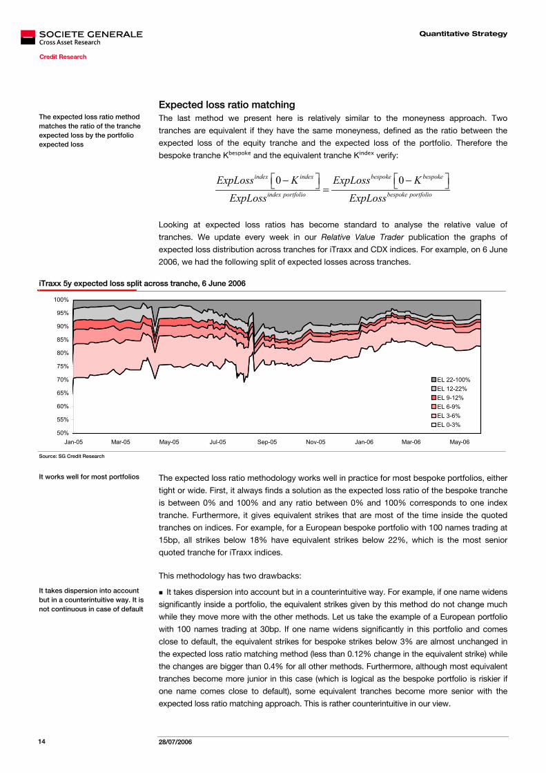
Looking at expected loss ratios has become standard to analyse the relative value of

tranches. We update every week in our Relative Value Trader publication the graphs of

expected loss distribution across tranches for iTraxx and CDX indices. For example, on 6 June

2006, we had the following split of expected losses across tranches.

iTraxx 5y expected loss split across tranche, 6 June 2006

50%

55%

60%

65%

70%

75%

80%

85%

90%

95%

100%

Jan-05 Mar-05 May-05 Jul-05 Sep-05 Nov-05 Jan-06 Mar-06 May-06

EL 22-100%EL 12-22%EL 9-12%EL 6-9%EL 3-6%EL 0-3%


The expected loss ratio methodology works well in practice for most bespoke portfolios, either

tight or wide. First, it always finds a solution as the expected loss ratio of the bespoke tranche

is between 0% and 100% and any ratio between 0% and 100% corresponds to one index

tranche. Furthermore, it gives equivalent strikes that are most of the time inside the quoted

tranches on indices. For example, for a European bespoke portfolio with 100 names trading at

15bp, all strikes below 18% have equivalent strikes below 22%, which is the most senior

quoted tranche for iTraxx indices.

This methodology has two drawbacks:

It takes dispersion into account but in a counterintuitive way. For example, if one name widens

significantly inside a portfolio, the equivalent strikes given by this method do not change much

while they move more with the other methods. Let us take the example of a European portfolio

with 100 names trading at 30bp. If one name widens significantly in this portfolio and comes

close to default, the equivalent strikes for bespoke strikes below 3% are almost unchanged in

the expected loss ratio matching method (less than 0.12% change in the equivalent strike) while

the changes are bigger than 0.4% for all other methods. Furthermore, although most equivalent

tranches become more junior in this case (which is logical as the bespoke portfolio is riskier if

one name comes close to default), some equivalent tranches become more senior with the

expected loss ratio matching approach. This is rather counterintuitive in our view.

It works well for most portfolios

The expected loss ratio method matches the ratio of the tranche expected loss by the portfolio expected loss

It takes dispersion into account but in a counterintuitive way. It is not continuous in case of default


28/07/2006 15

Another problem occurs when a name comes close to default. There is a jump in the

equivalent strike as soon as one name defaults like in the moneyness approach. Let us

consider once again the example of a bespoke [0-4%] tranche on a portfolio with 99 names at

30bp and one name at 50,000bp. The equivalent strike changes from 3.9% to 3.3% due to the

default of the risky name and this generates a +�80,000 P&L for a long �10m protection

position. Once again, this is a significant drawback for this method.

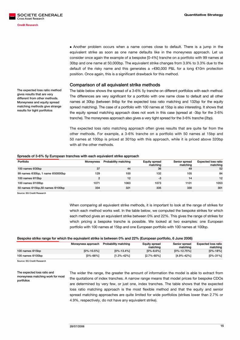
Comparison of all equivalent strike methods The table below shows the spread of a 3-6% 5y tranche on different portfolios with each method.

The differences are very significant for a portfolio with one name close to default and all other

names at 30bp (between 84bp for the expected loss ratio matching and 132bp for the equity

spread matching). The case of a portfolio with 100 names at 15bp is also interesting. It shows that

the equity spread matching approach does not work in this case (spread at -3bp for the 3-6%

tranche). The moneyness approach also gives a very tight spread for the 3-6% tranche (2bp).

The expected loss ratio matching approach often gives results that are quite far from the

other methods. For example, a 3-6% tranche on a portfolio with 50 names at 15bp and

50 names at 100bp is priced at 301bp with this approach, while it is priced above 320bp

with all the other methods.

Spreads of 3-6% 5y European tranches with each equivalent strike approach

Portfolio Moneyness Probability matching Equity spread matching

Senior spread matching

Expected loss ratio matching

100 names @30bp 37 44 36 49 52

99 names @30bp, 1 name @50000bp 129 100 132 105 84

100 names @15bp 2 12 -3 14 12

100 names @100bp 1071 1063 1073 1101 1053

50 names @15bp,50 names @100bp 334 321 335 330 301


When comparing all equivalent strike methods, it is important to look at the range of strikes for

which each method works well. In the table below, we computed the bespoke strikes for which

each method gives an equivalent strike between 0% and 22%. This gives the range of strikes for

which pricing a bespoke tranche is possible. We looked at two examples: one European

portfolio with 100 names at 15bp and one European portfolio with 100 names at 100bp.

Bespoke strike range for which the equivalent strike is between 0% and 22% (European portfolio, 6 June 2006)

Moneyness approach Probability matching Equity spread matching



100 names @15bp [0%-10.5%] [0%-13.4%] [0%-8.6%] [0%-12.75%] [0%-18%]

100 names @100bp [0%-66%] [1.3%-42%] [2.7%-60%] [4.9%-42%] [0%-31%]


The wider the range, the greater the amount of information the model is able to extract from

the quotations of index tranches. A narrow range means that model prices for bespoke CDOs

are determined by very few, or just one, index tranches. The table shows that the expected

loss ratio matching approach is the most flexible method and that the equity and senior

spread matching approaches are quite limited for wide portfolios (strikes lower than 2.7% or

4.9%, respectively, do not have any equivalent strike).

The expected loss ratio method gives results that are very different from other methods. Moneyness and equity spread matching methods give strange results for tight portfolios

The expected loss ratio and moneyness matching work for most portfolios


28/07/2006 16

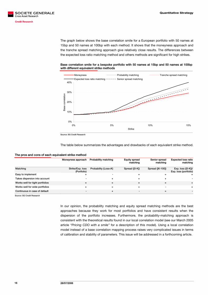
The graph below shows the base correlation smile for a European portfolio with 50 names at

15bp and 50 names at 100bp with each method. It shows that the moneyness approach and

the tranche spread matching approach give relatively close results. The differences between

the expected loss ratio matching method and others methods are significant for high strikes.

Base correlation smile for a bespoke portfolio with 50 names at 15bp and 50 names at 100bp with different equivalent strike methods

0%

10%

20%

30%

40%

0% 5% 10% 15%Strike

Bas

e co

rrela

tion

Moneyness Probability matching Tranche spread matchingExpected loss ratio matching Senior spread matching


The table below summarizes the advantages and drawbacks of each equivalent strike method.

The pros and cons of each equivalent strike method

Moneyness approach Probability matching Equity spread matching



Matching Strike/Exp. loss (Portfolio)

Probability (Loss<K) Spread ([0-K]) Spread ([K-100]) Exp. loss ([0-K])/ Exp. loss (portfolio)

Easy to implement + - = = =

Takes dispersion into account - + + + -

Works well for tight portfolios = = = = +

Works well for wide portfolios + = = - +

Continuous in case of default - + - = -


In our opinion, the probability matching and equity spread matching methods are the best

approaches because they work for most portfolios and have consistent results when the

dispersion of the portfolio increases. Furthermore, the probability-matching approach is

consistent with the theoretical results found in our local correlation model (see our March 2005

article “Pricing CDO with a smile” for a description of this model). Using a local correlation

model instead of a base correlation mapping process raises very complicated issues in terms

of calibration and stability of parameters. This issue will be addressed in a forthcoming article.


28/07/2006 17

Bespoke portfolios with several reference indices When a bespoke portfolio contains names linked to separate indices (for example European

and US names), the equivalent strike methodology needs to be refined to take into account

both correlation inputs. For the sake of simplicity, we look here at a Europe/US portfolio. We

present here three different methods to take into account several reference indices:

The separate weighted average method: the correlation assumption bespokeρ that is used for

the bespoke tranche is a weighted average of the correlations iTraxxρ and

CDXρ of the

equivalent strikes in the European and American smiles. The Europe and US equivalent strikes

are computed separately.

The joint weighted average method: the correlation assumption bespokeρ that is used for the

bespoke tranches is a weighted average of the correlations iTraxxρ and

CDXρ of the

equivalent strikes in the European and American smiles. The Europe and US equivalent strikes

are computed jointly.

The beta method: a beta is assigned to each name in the portfolio. This beta is the squared

root of the correlation of the equivalent strikes, i.e. iTraxx iTraxxβ ρ= ,

CDX CDXβ ρ= .

These three methods all rely on the methodology for finding the equivalent strike and

correlation in each region (Europe and US).

The separate weighted average method The separate weighted average method is relatively easy to implement. It assumes that the

correlation to use for the bespoke portfolio is a weighted average of the correlations of the

equivalent strikes in the Europe and US portfolios. The weights of the US and Europe

correlations depend on the percentage of the overall portfolio notional that is made of

European and US names.

The bespoke portfolio is first considered as 100% European to find the equivalent European

strike iTraxxK and correlation

iTraxxρ and then as a 100% US portfolio to find the equivalent

US strike CDXK and correlation

CDXρ . The bespoke correlation is then defined as the

weighted average of the two equivalent correlations:

(1 )bespoke iTraxx CDXEUR EURρ α ρ α ρ= + −

where EURα is the percentage of portfolio notional that is comprised of European names.

The weighted average method has two main drawbacks:

From a theoretical point of view, considering a mixed Europe/US portfolio as a 100%

European portfolio and then a 100% US portfolio is not satisfying. Using this method, the

equivalent CDX tranche is not equivalent to the equivalent iTraxx tranche. For example, with

the probability matching approach, the probability for the equivalent CDX tranche to get wiped

out is not equal to the probability for the equivalent iTraxx tranche to get wiped out.

This method applies the same correlation to all names when pricing the bespoke tranche

which is once again dissatisfying.

Three methods are used to analyse a bespoke portfolio with several reference indices

The separate weighted average method is the easiest to implement. It computes a weighted average of the Europe and US equivalent correlations

This method is the least satisfying from the theoretical point of view


28/07/2006 18

The joint weighted average method The joint weighted average method is a more sophisticated version of the separate weighted

average method. It also uses a weighted average of correlations to price the bespoke tranche

but it finds the equivalent Europe and US tranches at the same time. Therefore, it requires an

algorithm that finds both equivalent strikes jointly.

With the joint weighted average method, the two equivalent strikes iTraxxK and

CDXK are

found jointly so that the bespoke tranche priced with the correlation

(1 )bespoke iTraxx CDXEUR EURρ α ρ α ρ= + − is equivalent both to the iTraxx tranche

iTraxxK and the CDX tranche CDXK .

The joint weighted average gives results that are very close to the separate weighted average

method. The joint method ensures that equivalent Europe and US tranches are equivalent

between each other, which is satisfying from a theoretical point of view. For example, in the

joint probability matching method, the probability for the equivalent European tranche to get

wiped out is the same as the probability for the equivalent US strike to get wiped out.

When reference indices (here iTraxx and CDX) are fairly close and when their correlation smiles

are relatively close too, the separate and joint weighted average methods give very similar

results. Let us take the example of a 5y portfolio with 50 European names at 30bp and 50 US

names at 400bp. 0-3% tranches have exactly the same equivalent iTraxx and CDX tranches in

the joint and separate methods for all equivalent strike methods. For 0-15% tranches, there are

small differences between equivalent strikes (below 0.2% for all methods). Nevertheless, the

difference in equivalent correlations between joint and separate methods is less than 0.1%,

generating marked-to-market changes of about �2,000 for a �10m tranche notional.

The divergence between joint and separate methods is much higher when the reference

indices are very different. Let�s consider a bespoke portfolio mixing European Investment

Grade names and US High Yield names. In this case, it is possible to use the iTraxx Main and

CDX HY tranches as reference tranches. For a 0-15% tranche with 50 European names at

30bp (linked to the iTraxx index) and 50 US names at 400bp (linked to the CDX HY index), the

separate average method gives a 21.2% correlation while the joint average method gives a

20.36% correlation. This generates a �20,000 marked-to-market difference.

We do not recommend using the CDX HY as a reference index because its smile is very

volatile and leads to highly volatile valuations for bespoke tranches. Nevertheless, this

example shows that the two weighted average methods can give slightly different results.

The joint weighted average method computes the Europe and US equivalent strikes jointly. It then computes a weighted average of the two equivalent correlations

Separate and joint weighted average methods give very similar results


28/07/2006 19

The beta method Both weighted average methods have one theoretical flaw: they assign the same correlation to

European and US names in the bespoke portfolio. The beta method adjusts for this effect. It prices

the bespoke tranche with a beta assigned to each name. This beta is the same for all European

names (equal toiTraxx iTraxxβ ρ= ) and for all US names (equal to

CDX CDXβ ρ= ). Within

the Gaussian copula framework, the assets of the jth company write:

21j j j jA Xβ ε β= + −

with jε being the specific part of the assets of the jth company. These assets are simulated

and a default happens if they fall below a given threshold. This formula replaces:

1j jA Xρ ε ρ= + −

which corresponds to a homogeneous correlation ρ.

Using a homogeneous beta equal to the square root of correlation for all names is strictly

equivalent to using this correlation. Therefore finding two separate equivalent betas for Europe

and the US and then using a weighted average of these betas for the bespoke tranche is

perfectly equivalent to using the separate weighted average correlation method.

Here we use two different betas in the bespoke tranche. Therefore, the beta method

differentiates between European names and US names. In practice, the differences between

equivalent strikes in the beta and weighted average methods are small. As a case study, we

look at a 0-15% tranche on a portfolio with 50 European names at 30bp linked to the iTraxx

tranches and 50 US names at 400bp linked to the CDX HY tranches. The equivalent strikes

given by the beta method and the weighted average method differ by less than 0.2%. In terms

of mark-to-market, the differential is less than �10,000 for a notional of �10m. If the 400bp

names are linked to the CDX HY tranches, the divergence is bigger both on strikes (1.1%

differences between equivalent strikes in the weighted average and beta methods) and on

valuations (up to �200,000 differences for a �10m notional).

The beta method assigns a different beta to European and US names

The beta method is the most satisfying from the theoretical point of view. Results are relatively close to the results of the two other methods


28/07/2006 20

SG Quantitative Credit Strategy past publications

June 2006 A primer on CPPI

May 2006 The quest for a better firm model: estimating jump-to-default out of the equity volatility smile

April 2006 Looking for value in the Bank Tier 1 market

April 2006 Finding the fair spread of credit indices

March 2006 Taking advantage of LBO speculation

March 2006 Building correlation trades: a case study

February 2006 CDO²: new opportunities

December 2005 Looking for value in the sub insurance market

November 2005 The wise man is he who knows the relative value of things

October 2005 Do corporate hybrids offer value?

September 2005 Playing long term bonds against 10yr CDS

July 2005 Local correlation: a backtesting study

June 2005 A note on the distribution of asset value in the local correlation model

May 2005 Hedging CDS curve trades: a case study

April 2005 CMCDS: sense and sensitivity

March 2005 The basics of spread option pricing

February 2005 The relative value of EDS against credit and equity derivatives

February 2005 Pricing CDOs with a smile

November 2004 Introducing the CDS Curves Monitor

October 2004 Empirical evidence on the BFM model

September 2004 CDS vs. Stock – the quest for the optimum hedge ratio

July 2004 Pricing and hedging of correlation products

July 2004 The new iTraxx indices

April 2004 A hedging model for capital structure arbitrage

March 2004 Back to basics: which spread for measuring credit?

January 2004 Backtesting basis trades: a case study

December 2003 Forecasting the iBoxx Diversified CDS index

October 2003 Kohonen maps: going beyond classification for enhanced management strategies

September 2003 Arbitrage between credits and equities – new strategies, more opportunities

August 2003 Pricing the basis

July 2003 Hedging bonds using CDS and taking advantage of convexity

June 2003 Firm models with event risk

May 2003 Beta-neutral relative value analysis

April 2003 Arbitrage between CDS and bonds

March 2003 Forecasting individual corporate credit spreads

December 2002 2002: of useful models

October 2002 Firm models and trading strategies (2)

September 2002 Firm models and trading strategies (1)

July 2002 Backtesting systematic Rich/Cheap strategies

June 2002 An analysis of CDO downgrades

May 2002 How to optimize a credit portfolio

April 2002 CDOs as balance sheet management tools

March 2002 A spread forecasting model

February 2002 Cash-flow CDOs – highly enhanced assets

January 2002 Beyond volatility and correlation

November 2001 Some applications of a firm value model

October 2001 Why can a credit curve invert?

September 2001 Looking for value on the European Credit Market

September 2001 Pricing put options indexed on ratings

July 2001 A smile model for valuing capital securities

June 2001 Understanding the dynamics of Credit Spreads

May 2001 What are the incentives to use internal ratings in the new Cooke ratio?

April 2001 A rule-of-thumb for valuing Telecom coupon step-ups

March 2001 How does the market reward the risks of default or rating downgrade?


The information herein is not intended to be an offer to buy or sell, or a solicitation of an offer to buy or sell, any securities and including any expression of opinion, has been obtained from

or is based upon sources believed to be reliable but is not guaranteed as to accuracy or completeness although Société Générale (�SG�) believe it to be fair and not misleading or

deceptive. SG, and their affiliated companies in the SG Group, may from time to time deal in, profit from the trading of, hold or act as market-makers or act as advisers, brokers or bankers

in relation to the securities, or derivatives thereof, of persons, firms or entities mentioned in this document or be represented on the board of such persons, firms or entities. Employees of

SG, and their affiliated companies in the SG Group, or individuals connected to then, other than the authors of this report, may from time to time have a position in or be holding any of the

investments or related investments mentioned in this document. Each author of this report is not permitted to trade in or hold any of the investments or related investments which are the

subject of this document. SG and their affiliated companies in the SG Group are under no obligation to disclose or take account of this document when advising or dealing with or for their

customers. The views of SG reflected in this document may change without notice. To the maximum extent possible at law, SG does not accept any liability whatsoever arising from the

use of the material or information contained herein. This research document is not intended for use by or targeted at private customers. Should a private customer obtain a copy of this

report they should not base their investment decisions solely on the basis of this document but must seek independent financial advice.

IMPORTANT DISCLOSURES: Please refer to our website: http:\\www.sgresearch.socgen.com

This publication is issued in France by or through Société Générale ("SG�) which is regulated by the AMF (Autorité des Marchés Financiers).

Notice to UK Investors: This publication is issued in the United Kingdom by or through Société Générale ("SG"). All materials provided by SG Commodity Research and SG Global

Convertible Research are produced in circumstances such that it is not appropriate to characterize them as impartial as referred to in the Financial Services Authority Handbook. However,

it must be made clear that all research issued by SG will be fair, clear and not misleading. SG is a Member of the London Stock Exchange. Notice to US Investors: This report is issued solely to major US institutional investors pursuant to SEC Rule 15a-6. Any US person wishing to discuss this report or effect transactions in

any security discussed herein should do so with or through SG Americas Securities, LLC to conform with the requirements of US securities law. SG Americas Securities, LLC, 1221 Avenue

of the Americas, New York, NY, 10020. (212) 278-6000. Some of the securities mentioned herein may not be qualified for sale under the securities laws of certain states, except for

unsolicited orders. Customer purchase orders made on the basis of this report cannot be considered to be unsolicited by SG Americas Securities, LLC and therefore may not be accepted

by SG Americas Securities, LLC investment executives unless the security is qualified for sale in the state.

Analyst Certification: Each author of this research report hereby certifies that (i) the views expressed in the research report accurately reflect his or her personal views about any and all of

the subject securities or issuers and (ii) no part of his or her compensation was, is, or will be related, directly or indirectly, to the specific recommendations or views expressed in this

report.

Notice to Japanese Investors: This report is distributed in Japan by Société Générale Securities (North Pacific) Ltd., Tokyo Branch, which is regulated by the Financial Services Agency of

Japan. The products mentioned in this report may not be eligible for sale in Japan and they may not be suitable for all types of investors.

Notice to Australian Investors: Société Générale Australia Branch (ABN 71 092 516 286) (SG) takes responsibility for publishing this document. SG holds an AFSL no. 236651 issued

under the Corporations Act 2001 (Cth) ("Act"). The information contained in this newsletter is only directed to recipients who are wholesale clients as defined under the Act. hhtp://www.sgcib.com. Copyright: The Société Générale Group 2006. All rights reserved

Credit, Fixed Income & Forex Research

Global Head of Credit, Fixed Income & Forex Research Benoît Hubaud (33) 1 42 13 61 08 / (44) 20 7676 7168

Research Manager Denis Groven (33) 1 42 13 78 21 Quant Research

Head Julien Turc (33) 1 42 13 40 90

David Benhamou (33) 1 42 13 94 75

Credit Research Benjamin Herzog (33) 1 42 13 67 49

Auto & Transportation Pierre Bergeron (33) 1 42 13 89 15 Marc Teyssier (33) 1 42 13 55 96

Stéphanie Herrault (33) 1 42 13 63 11

Credit Strategy

Consumers & Services Sonia van Dorp (33) 1 42 13 64 57 Suki Mann (44) 20 7676 7063

Olivier Monnoyeur, CFA (33) 1 42 13 43 87 Guy Stear, CFA (33) 1 42 13 40 26

Industrials Roberto Pozzi (44) 20 7676 7152 Fixed & Forex Strategy

Ozana Breaban (44) 20 7676 7160 Head Vincent Chaigneau (44) 20 7676 7707

Telecom & Media Satyajit Chatterjee (44) 20 7676 7023 Fixed Income Adam Kurpiel (44) 20 7676 7708

Terry Nguyen, CFA (44) 20 7676 7162 Khrishnamoorthy Sooben (44) 20 7676 7713

Ciaran O'Hagan (33) 1 42 13 58 60

Aro Razafindrakola (33) 1 42 13 64 93

Utilities Hervé Gay (33) 1 42 13 87 50 Jose Sarafana (33) 1 42 13 56 59

Florence Roche (33) 1 42 13 63 99 Guillaume Baron (33) 1 42 13 57 07

Banks & Insurance Robert Montague (44) 20 7676 7062 Foreign Exchange Niels Christensen (33) 1 42 13 90 77

Eleanor Yeh (44) 20 7676 7030 Carole Laulhere (33) 1 42 13 71 45

Julien Martin (44) 20 7676 7262 Murat Toprak (33) 1 42 13 39 68

Benjamin Freoa (33) 1 42 13 71 29

High Yield Julien Raffelsbauer, CFA (44) 20 7676 7059

Jostein Gauslaa (44) 20 7676 7158 Technical Analysis Hughes Naka (33) 1 42 13 51 10

Stephane Billioud (33) 1 42 13 35 55

ABS Jean-David Cirotteau (33) 1 42 13 72 52

Alexander Mackay (44) 20 7676 7055

Asian Risks Sabine Ko (852) 21 66 57 67

Daniel Tam (852) 21 66 56 61

Paris Tour Société Générale 17 cours Valmy 92987 Paris La Défense Cedex - France

London SG House – 41, Tower Hill London EC3 N 4SG United Kingdom

Hong Kong Level 38, Pacific Place 1 Queen's Road East Hong Kong

socgen quant strategy - pricing bespoke cdos

Documents

bespoke portfolios

moneyness matching

base correlation surface

base correlation smile

senior spread matching

smiles of base correlation

correlation desks

expected loss ratio