soa exam p - actuarial bookstore · • actuarial exam & career ... 3.the probability of a...
TRANSCRIPT
Actuarial Study MaterialsLearning Made Easier
StudyPlus+ gives you digital access* to:• Flashcards & Formula Sheet
• Actuarial Exam & Career Strategy Guides
• Technical Skill eLearning Tools
• Samples of Supplemental Textbooks
• And more!
*See inside for keycode access and login instructions
With StudyPlus+
SOA Exam PStudy Manual
2nd EditionAbraham Weishaus, Ph.D., F.S.A., CFA, M.A.A.A.
NO RETURN IF OPENED
Contents
Introduction vii
Calculus Notes xi
1 Sets 1Exercises . . . . . . . . . . . . . . . . . . . . . . . . . . . . . . . . . . . . . . . . . 5Solutions . . . . . . . . . . . . . . . . . . . . . . . . . . . . . . . . . . . . . . . . . 13
2 Combinatorics 19Exercises . . . . . . . . . . . . . . . . . . . . . . . . . . . . . . . . . . . . . . . . . 24Solutions . . . . . . . . . . . . . . . . . . . . . . . . . . . . . . . . . . . . . . . . . 28
3 Conditional Probability 33Exercises . . . . . . . . . . . . . . . . . . . . . . . . . . . . . . . . . . . . . . . . . 34Solutions . . . . . . . . . . . . . . . . . . . . . . . . . . . . . . . . . . . . . . . . . 40
4 Bayes’ Theorem 47Exercises . . . . . . . . . . . . . . . . . . . . . . . . . . . . . . . . . . . . . . . . . 49Solutions . . . . . . . . . . . . . . . . . . . . . . . . . . . . . . . . . . . . . . . . . 54
5 Random Variables 595.1 Insurance random variables . . . . . . . . . . . . . . . . . . . . . . . . . . . . . . 63
Exercises . . . . . . . . . . . . . . . . . . . . . . . . . . . . . . . . . . . . . . . . . 64Solutions . . . . . . . . . . . . . . . . . . . . . . . . . . . . . . . . . . . . . . . . . 68
6 Conditional Probability for Random Variables 73Exercises . . . . . . . . . . . . . . . . . . . . . . . . . . . . . . . . . . . . . . . . . 74Solutions . . . . . . . . . . . . . . . . . . . . . . . . . . . . . . . . . . . . . . . . . 78
7 Mean 83Exercises . . . . . . . . . . . . . . . . . . . . . . . . . . . . . . . . . . . . . . . . . 88Solutions . . . . . . . . . . . . . . . . . . . . . . . . . . . . . . . . . . . . . . . . . 94
8 Variance and other Moments 1038.1 Bernoulli shortcut . . . . . . . . . . . . . . . . . . . . . . . . . . . . . . . . . . . . 105
Exercises . . . . . . . . . . . . . . . . . . . . . . . . . . . . . . . . . . . . . . . . . 107Solutions . . . . . . . . . . . . . . . . . . . . . . . . . . . . . . . . . . . . . . . . . 112
9 Percentiles 117Exercises . . . . . . . . . . . . . . . . . . . . . . . . . . . . . . . . . . . . . . . . . 118Solutions . . . . . . . . . . . . . . . . . . . . . . . . . . . . . . . . . . . . . . . . . 121
P Study Manual—2nd editionCopyright ©2017 ASM
iii
iv CONTENTS
10 Mode 125Exercises . . . . . . . . . . . . . . . . . . . . . . . . . . . . . . . . . . . . . . . . . 126Solutions . . . . . . . . . . . . . . . . . . . . . . . . . . . . . . . . . . . . . . . . . 129
11 Joint Distribution 13511.1 Independent random variables . . . . . . . . . . . . . . . . . . . . . . . . . . . . 13511.2 Joint distribution of two random variables . . . . . . . . . . . . . . . . . . . . . . 135
Exercises . . . . . . . . . . . . . . . . . . . . . . . . . . . . . . . . . . . . . . . . . 139Solutions . . . . . . . . . . . . . . . . . . . . . . . . . . . . . . . . . . . . . . . . . 146
12 Uniform Distribution 153Exercises . . . . . . . . . . . . . . . . . . . . . . . . . . . . . . . . . . . . . . . . . 156Solutions . . . . . . . . . . . . . . . . . . . . . . . . . . . . . . . . . . . . . . . . . 160
13 Marginal Distribution 169Exercises . . . . . . . . . . . . . . . . . . . . . . . . . . . . . . . . . . . . . . . . . 170Solutions . . . . . . . . . . . . . . . . . . . . . . . . . . . . . . . . . . . . . . . . . 173
14 Joint Moments 177Exercises . . . . . . . . . . . . . . . . . . . . . . . . . . . . . . . . . . . . . . . . . 178Solutions . . . . . . . . . . . . . . . . . . . . . . . . . . . . . . . . . . . . . . . . . 185
15 Covariance 197Exercises . . . . . . . . . . . . . . . . . . . . . . . . . . . . . . . . . . . . . . . . . 200Solutions . . . . . . . . . . . . . . . . . . . . . . . . . . . . . . . . . . . . . . . . . 206
16 Conditional Distribution 213Exercises . . . . . . . . . . . . . . . . . . . . . . . . . . . . . . . . . . . . . . . . . 215Solutions . . . . . . . . . . . . . . . . . . . . . . . . . . . . . . . . . . . . . . . . . 221
17 Conditional Moments 231Exercises . . . . . . . . . . . . . . . . . . . . . . . . . . . . . . . . . . . . . . . . . 232Solutions . . . . . . . . . . . . . . . . . . . . . . . . . . . . . . . . . . . . . . . . . 237
18 Double Expectation Formulas 245Exercises . . . . . . . . . . . . . . . . . . . . . . . . . . . . . . . . . . . . . . . . . 247Solutions . . . . . . . . . . . . . . . . . . . . . . . . . . . . . . . . . . . . . . . . . 251
19 Binomial Distribution 25919.1 Binomial Distribution . . . . . . . . . . . . . . . . . . . . . . . . . . . . . . . . . . 25919.2 Hypergeometric Distribution . . . . . . . . . . . . . . . . . . . . . . . . . . . . . 26019.3 Trinomial Distribution . . . . . . . . . . . . . . . . . . . . . . . . . . . . . . . . . 261
Exercises . . . . . . . . . . . . . . . . . . . . . . . . . . . . . . . . . . . . . . . . . 262Solutions . . . . . . . . . . . . . . . . . . . . . . . . . . . . . . . . . . . . . . . . . 269
20 Negative Binomial Distribution 277
P Study Manual—2nd editionCopyright ©2017 ASM
CONTENTS v
Exercises . . . . . . . . . . . . . . . . . . . . . . . . . . . . . . . . . . . . . . . . . 279Solutions . . . . . . . . . . . . . . . . . . . . . . . . . . . . . . . . . . . . . . . . . 284
21 Poisson Distribution 291Exercises . . . . . . . . . . . . . . . . . . . . . . . . . . . . . . . . . . . . . . . . . 292Solutions . . . . . . . . . . . . . . . . . . . . . . . . . . . . . . . . . . . . . . . . . 296
22 Exponential Distribution 303Exercises . . . . . . . . . . . . . . . . . . . . . . . . . . . . . . . . . . . . . . . . . 306Solutions . . . . . . . . . . . . . . . . . . . . . . . . . . . . . . . . . . . . . . . . . 313
23 Normal Distribution 323Exercises . . . . . . . . . . . . . . . . . . . . . . . . . . . . . . . . . . . . . . . . . 326Solutions . . . . . . . . . . . . . . . . . . . . . . . . . . . . . . . . . . . . . . . . . 331
24 Bivariate Normal Distribution 339Exercises . . . . . . . . . . . . . . . . . . . . . . . . . . . . . . . . . . . . . . . . . 341Solutions . . . . . . . . . . . . . . . . . . . . . . . . . . . . . . . . . . . . . . . . . 344
25 Central Limit Theorem 349Exercises . . . . . . . . . . . . . . . . . . . . . . . . . . . . . . . . . . . . . . . . . 352Solutions . . . . . . . . . . . . . . . . . . . . . . . . . . . . . . . . . . . . . . . . . 355
26 Order Statistics 361Exercises . . . . . . . . . . . . . . . . . . . . . . . . . . . . . . . . . . . . . . . . . 364Solutions . . . . . . . . . . . . . . . . . . . . . . . . . . . . . . . . . . . . . . . . . 368
27 Moment Generating Function 373Exercises . . . . . . . . . . . . . . . . . . . . . . . . . . . . . . . . . . . . . . . . . 376Solutions . . . . . . . . . . . . . . . . . . . . . . . . . . . . . . . . . . . . . . . . . 381
28 Probability Generating Function 389Exercises . . . . . . . . . . . . . . . . . . . . . . . . . . . . . . . . . . . . . . . . . 393Solutions . . . . . . . . . . . . . . . . . . . . . . . . . . . . . . . . . . . . . . . . . 394
29 Transformations 397Exercises . . . . . . . . . . . . . . . . . . . . . . . . . . . . . . . . . . . . . . . . . 399Solutions . . . . . . . . . . . . . . . . . . . . . . . . . . . . . . . . . . . . . . . . . 403
30 Transformations of Two or More Variables 409Exercises . . . . . . . . . . . . . . . . . . . . . . . . . . . . . . . . . . . . . . . . . 411Solutions . . . . . . . . . . . . . . . . . . . . . . . . . . . . . . . . . . . . . . . . . 415
P Study Manual—2nd editionCopyright ©2017 ASM
vi CONTENTS
Practice Exams 423
1 Practice Exam 1 425
2 Practice Exam 2 433
3 Practice Exam 3 441
4 Practice Exam 4 449
5 Practice Exam 5 457
6 Practice Exam 6 465
Appendices 473
A Solutions to the Practice Exams 475Solutions for Practice Exam 1 . . . . . . . . . . . . . . . . . . . . . . . . . . . . . . . . 475Solutions for Practice Exam 2 . . . . . . . . . . . . . . . . . . . . . . . . . . . . . . . . 483Solutions for Practice Exam 3 . . . . . . . . . . . . . . . . . . . . . . . . . . . . . . . . 491Solutions for Practice Exam 4 . . . . . . . . . . . . . . . . . . . . . . . . . . . . . . . . 501Solutions for Practice Exam 5 . . . . . . . . . . . . . . . . . . . . . . . . . . . . . . . . 511Solutions for Practice Exam 6 . . . . . . . . . . . . . . . . . . . . . . . . . . . . . . . . 520
B Exam Question Index 533
P Study Manual—2nd editionCopyright ©2017 ASM
Lesson 1
Sets
Most things in life are not certain. Probability is a mathematical model for uncertain events.Probability assigns a number between 0 and 1 to each event. This numbermay have the followingmeanings:
1. It may indicate that of all the events in the universe, the proportion of them included inthis event is that number. For example, if one says that 70% of the population owns a car,it means that the number of people owning a car is 70% of the number of people in thepopulation.
2. It may indicate that in the long run, this event will occur that proportion of the time. Forexample, if we say that a certain medicine cures an illness 80% of the time, it means thatwe expect that if we have a large number of people, let’s say 1000, with that illness whotake the medicine, approximately 800 will be cured.
From a mathematical viewpoint, probability is a function from the space of events to theinterval of real numbers between 0 and 1. We write this function as P[A], where A is an event.We often want to study combinations of events. For example, if we are studying people, eventsmay be “male”, “female”, “married”, and “single”. But we may also want to consider the event“young and married”, or “male or single”. To understand how to manipulate combinations ofevents, let’s briefly study set theory. An event can be treated as a set.
A set is a collection of objects. The objects in the set are called members of the set. Twospecial sets are
1. The entire space. I’ll use Ω for the entire space, but there is no standard notation. Allmembers of all sets must come from Ω.
2. The empty set, usually denoted by . This set has no members.
There are three important operations on sets:
Union If A and B are sets, we write the union as A ∪ B. It is defined as the set whose membersare all the members of A plus all the members of B. Thus if x is in A ∪ B, then either x isin A or x is in B. x may be a member of both A and B. The union of two sets is always atleast as large as each of the two component sets.
Intersection If A and B are sets, we write the intersection as A∩B. It is defined as the set whosemembers are in both A and B. The intersection of two sets is always no larger than each ofthe two component sets.
Complement If A is a set, its complement is the set of members ofΩ that are not members of A.There is no standard notation for complement; different textbooks use A′, Ac , and A. I’lluse A′, the notation used in SOA sample questions. Interestingly, SOA sample solutionsuse Ac instead.
P Study Manual—2nd editionCopyright ©2017 ASM
1
2 1. SETS
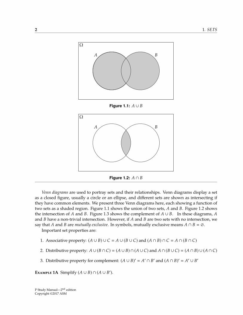
Ω
A B
Figure 1.1: A ∪ B
Ω
A B
Figure 1.2: A ∩ B
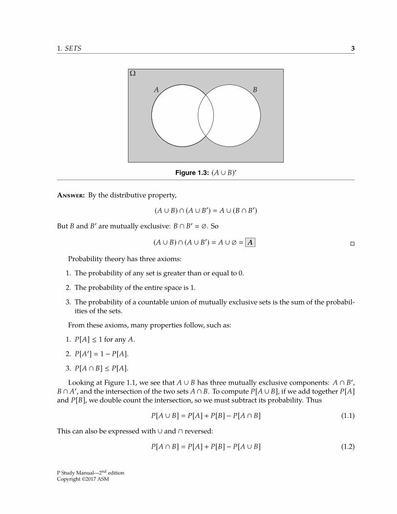
Venn diagrams are used to portray sets and their relationships. Venn diagrams display a setas a closed figure, usually a circle or an ellipse, and different sets are shown as intersecting ifthey have common elements. We present three Venn diagrams here, each showing a function oftwo sets as a shaded region. Figure 1.1 shows the union of two sets, A and B. Figure 1.2 showsthe intersection of A and B. Figure 1.3 shows the complement of A ∪ B. In these diagrams, Aand B have a non-trivial intersection. However, if A and B are two sets with no intersection, wesay that A and B are mutually exclusive. In symbols, mutually exclusive means A ∩ B .
Important set properties are:
1. Associative property: (A ∪ B) ∪ C A ∪ (B ∪ C) and (A ∩ B) ∩ C A ∩ (B ∩ C)
2. Distributive property: A ∪ (B ∩ C) (A ∪ B) ∩ (A ∪ C) and A ∩ (B ∪ C) (A ∩ B) ∪ (A ∩ C)
3. Distributive property for complement: (A ∪ B)′ A′ ∩ B′ and (A ∩ B)′ A′ ∪ B′
Example 1A Simplify (A ∪ B) ∩ (A ∪ B′).
P Study Manual—2nd editionCopyright ©2017 ASM
1. SETS 3
Ω
A B
Figure 1.3: (A ∪ B)′
Answer: By the distributive property,
(A ∪ B) ∩ (A ∪ B′) A ∪ (B ∩ B′)But B and B′ are mutually exclusive: B ∩ B′ . So
(A ∪ B) ∩ (A ∪ B′) A ∪ A
Probability theory has three axioms:
1. The probability of any set is greater than or equal to 0.
2. The probability of the entire space is 1.
3. The probability of a countable union of mutually exclusive sets is the sum of the probabil-ities of the sets.
From these axioms, many properties follow, such as:
1. P[A] ≤ 1 for any A.
2. P[A′] 1 − P[A].3. P[A ∩ B] ≤ P[A].Looking at Figure 1.1, we see that A ∪ B has three mutually exclusive components: A ∩ B′,
B ∩A′, and the intersection of the two sets A ∩ B. To compute P[A ∪ B], if we add together P[A]and P[B], we double count the intersection, so we must subtract its probability. Thus
P[A ∪ B] P[A] + P[B] − P[A ∩ B] (1.1)
This can also be expressed with ∪ and ∩ reversed:
P[A ∩ B] P[A] + P[B] − P[A ∪ B] (1.2)
P Study Manual—2nd editionCopyright ©2017 ASM
4 1. SETS
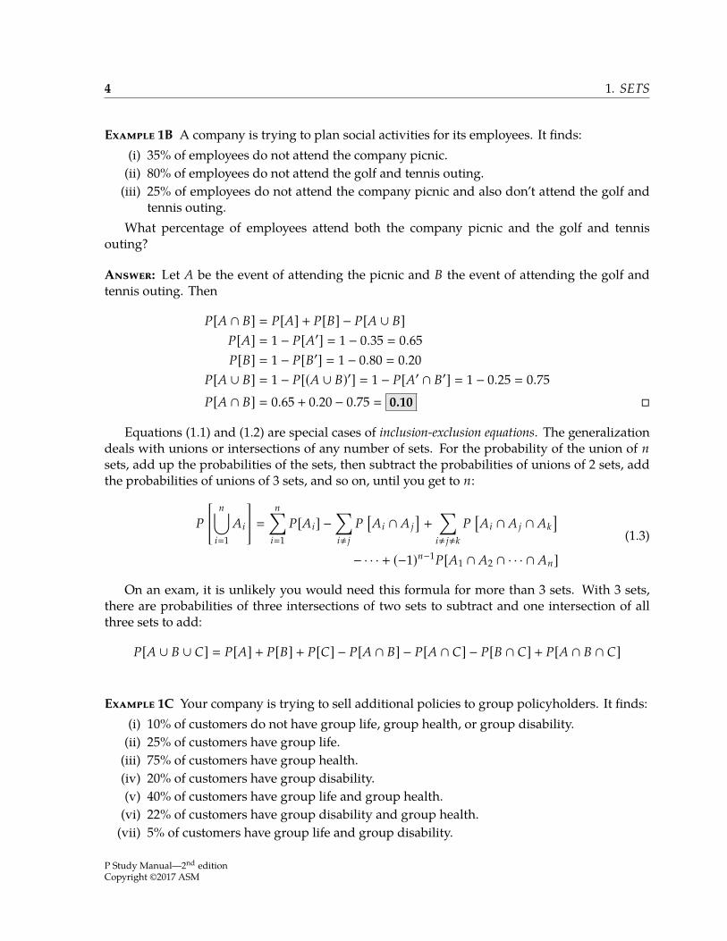
Example 1B A company is trying to plan social activities for its employees. It finds:(i) 35% of employees do not attend the company picnic.(ii) 80% of employees do not attend the golf and tennis outing.(iii) 25% of employees do not attend the company picnic and also don’t attend the golf and
tennis outing.What percentage of employees attend both the company picnic and the golf and tennis
outing?
Answer: Let A be the event of attending the picnic and B the event of attending the golf andtennis outing. Then
P[A ∩ B] P[A] + P[B] − P[A ∪ B]P[A] 1 − P[A′] 1 − 0.35 0.65P[B] 1 − P[B′] 1 − 0.80 0.20
P[A ∪ B] 1 − P[(A ∪ B)′] 1 − P[A′ ∩ B′] 1 − 0.25 0.75P[A ∩ B] 0.65 + 0.20 − 0.75 0.10
Equations (1.1) and (1.2) are special cases of inclusion-exclusion equations. The generalizationdeals with unions or intersections of any number of sets. For the probability of the union of nsets, add up the probabilities of the sets, then subtract the probabilities of unions of 2 sets, addthe probabilities of unions of 3 sets, and so on, until you get to n:
P
[n⋃
i1Ai
]
n∑i1
P[Ai] −∑i, j
P[Ai ∩ A j
]+
∑i, j,k
P[Ai ∩ A j ∩ Ak
]− · · · + (−1)n−1P[A1 ∩ A2 ∩ · · · ∩ An]
(1.3)
On an exam, it is unlikely you would need this formula for more than 3 sets. With 3 sets,there are probabilities of three intersections of two sets to subtract and one intersection of allthree sets to add:
P[A ∪ B ∪ C] P[A] + P[B] + P[C] − P[A ∩ B] − P[A ∩ C] − P[B ∩ C] + P[A ∩ B ∩ C]
Example 1C Your company is trying to sell additional policies to group policyholders. It finds:(i) 10% of customers do not have group life, group health, or group disability.(ii) 25% of customers have group life.(iii) 75% of customers have group health.(iv) 20% of customers have group disability.(v) 40% of customers have group life and group health.(vi) 22% of customers have group disability and group health.(vii) 5% of customers have group life and group disability.
P Study Manual—2nd editionCopyright ©2017 ASM
EXERCISES FOR LESSON 1 5
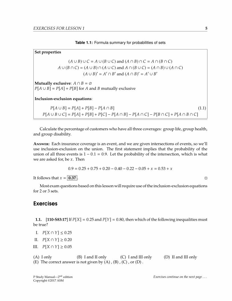
Table 1.1: Formula summary for probabilities of sets
Set properties
(A ∪ B) ∪ C A ∪ (B ∪ C) and (A ∩ B) ∩ C A ∩ (B ∩ C)A ∪ (B ∩ C) (A ∪ B) ∩ (A ∪ C) and A ∩ (B ∪ C) (A ∩ B) ∪ (A ∩ C)
(A ∪ B)′ A′ ∩ B′ and (A ∩ B)′ A′ ∪ B′
Mutually exclusive: A ∩ B P[A ∪ B] P[A] + P[B] for A and B mutually exclusive
Inclusion-exclusion equations:
P[A ∪ B] P[A] + P[B] − P[A ∩ B] (1.1)P[A ∪ B ∪ C] P[A] + P[B] + P[C] − P[A ∩ B] − P[A ∩ C] − P[B ∩ C] + P[A ∩ B ∩ C]
Calculate the percentage of customers who have all three coverages: group life, group health,and group disability.
Answer: Each insurance coverage is an event, and we are given intersections of events, so we’lluse inclusion-exclusion on the union. The first statement implies that the probability of theunion of all three events is 1 − 0.1 0.9. Let the probability of the intersection, which is whatwe are asked for, be x. Then
0.9 0.25 + 0.75 + 0.20 − 0.40 − 0.22 − 0.05 + x 0.53 + x
It follows that x 0.37 .
Most examquestions basedon this lessonwill requireuse of the inclusion-exclusion equationsfor 2 or 3 sets.
Exercises
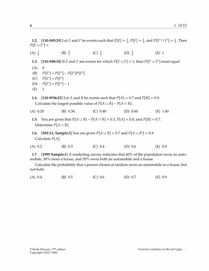
1.1. [110-S83:17] If P[X] 0.25 and P[Y] 0.80, thenwhich of the following inequalities mustbe true?
I. P[X ∩ Y] ≤ 0.25II. P[X ∩ Y] ≥ 0.20III. P[X ∩ Y] ≥ 0.05
(A) I only (B) I and II only (C) I and III only (D) II and III only(E) The correct answer is not given by (A) , (B) , (C) , or (D) .
P Study Manual—2nd editionCopyright ©2017 ASM
Exercises continue on the next page . . .
6 1. SETS
1.2. [110-S85:29] Let E and F be events such that P[E] 12 , P[F] 1
2 , and P[E′ ∩ F′] 13 . Then
P[E ∪ F′] (A) 1
4 (B) 23 (C) 3
4 (D) 56 (E) 1
1.3. [110-S88:10] If E and F are events for which P[E ∪ F] 1, then P[E′ ∪ F′]must equal(A) 0(B) P[E′] + P[F′] − P[E′]P[F′](C) P[E′] + P[F′](D) P[E′] + P[F′] − 1(E) 1
1.4. [110-W96:23] Let A and B be events such that P[A] 0.7 and P[B] 0.9.Calculate the largest possible value of P[A ∪ B] − P[A ∩ B].
(A) 0.20 (B) 0.34 (C) 0.40 (D) 0.60 (E) 1.60
1.5. You are given that P[A ∪ B] − P[A ∩ B] 0.3, P[A] 0.8, and P[B] 0.7.Determine P[A ∪ B].
1.6. [S01:12, Sample:3] You are given P[A ∪ B] 0.7 and P[A ∪ B′] 0.9.Calculate P[A].
(A) 0.2 (B) 0.3 (C) 0.4 (D) 0.6 (E) 0.8
1.7. [1999 Sample:1] A marketing survey indicates that 60% of the population owns an auto-mobile, 30% owns a house, and 20% owns both an automobile and a house.
Calculate the probability that a person chosen at random owns an automobile or a house, butnot both.
(A) 0.4 (B) 0.5 (C) 0.6 (D) 0.7 (E) 0.9
P Study Manual—2nd editionCopyright ©2017 ASM
Exercises continue on the next page . . .
EXERCISES FOR LESSON 1 7
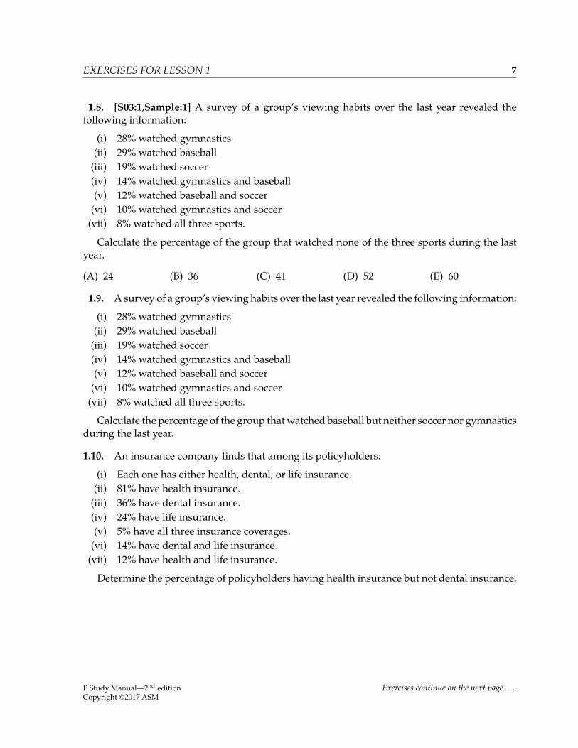
1.8. [S03:1,Sample:1] A survey of a group’s viewing habits over the last year revealed thefollowing information:
(i) 28% watched gymnastics(ii) 29% watched baseball(iii) 19% watched soccer(iv) 14% watched gymnastics and baseball(v) 12% watched baseball and soccer(vi) 10% watched gymnastics and soccer(vii) 8% watched all three sports.
Calculate the percentage of the group that watched none of the three sports during the lastyear.
(A) 24 (B) 36 (C) 41 (D) 52 (E) 60
1.9. A survey of a group’s viewing habits over the last year revealed the following information:
(i) 28% watched gymnastics(ii) 29% watched baseball(iii) 19% watched soccer(iv) 14% watched gymnastics and baseball(v) 12% watched baseball and soccer(vi) 10% watched gymnastics and soccer(vii) 8% watched all three sports.
Calculate the percentage of the group thatwatched baseball but neither soccer nor gymnasticsduring the last year.
1.10. An insurance company finds that among its policyholders:
(i) Each one has either health, dental, or life insurance.(ii) 81% have health insurance.(iii) 36% have dental insurance.(iv) 24% have life insurance.(v) 5% have all three insurance coverages.(vi) 14% have dental and life insurance.(vii) 12% have health and life insurance.
Determine the percentage of policyholders having health insurance but not dental insurance.
P Study Manual—2nd editionCopyright ©2017 ASM
Exercises continue on the next page . . .
8 1. SETS
1.11. [S00:1,Sample:2] The probability that a visit to a primary care physician’s (PCP) officeresults in neither lab work nor referral to a specialist is 35% . Of those coming to a PCP’s office,30% are referred to specialists and 40% require lab work.
Calculate the probability that a visit to a PCP’s office results in both lab work and referral toa specialist.
(A) 0.05 (B) 0.12 (C) 0.18 (D) 0.25 (E) 0.35
1.12. In a certain town, there are 1000 cars. All cars are white, blue, or gray, and are eithersedans or SUVs. There are 300 white cars, 400 blue cars, 760 sedans, 180 white sedans, and 320blue sedans.
Determine the number of gray SUVs.
1.13. [F00:3,Sample:5]An auto insurance companyhas 10,000policyholders. Eachpolicyholderis classified as
(i) young or old;(ii) male or female; and(iii) married or single
Of these policyholders, 3000 are young, 4600 are male, and 7000 are married. The policy-holders can also be classified as 1320 young males, 3010 married males, and 1400 young marriedpersons. Finally, 600 of the policyholders are young married males.
Calculate the number of the company’s policyholders who are young, female, and single.
(A) 280 (B) 423 (C) 486 (D) 880 (E) 896
1.14. An auto insurance company has 10,000 policyholders. Each policyholder is classified as
(i) young or old;(ii) male or female; and(iii) married or single
Of these policyholders, 4000 are young, 5600 are male, and 3500 are married. The policy-holders can also be classified as 2820 young males, 1540 married males, and 1300 young marriedpersons. Finally, 670 of the policyholders are young married males.
How many of the company’s policyholders are old, female, and single?
1.15. [F01:9,Sample:8] Among a large group of patients recovering from shoulder injuries, it isfound that 22% visit both a physical therapist and a chiropractor, whereas 12% visit neither ofthese. The probability that a patient visits a chiropractor exceeds by 0.14 the probability that apatient visits a physical therapist.
Calculate the probability that a randomly chosen member of this group visits a physicaltherapist.
(A) 0.26 (B) 0.38 (C) 0.40 (D) 0.48 (E) 0.62
P Study Manual—2nd editionCopyright ©2017 ASM
Exercises continue on the next page . . .
EXERCISES FOR LESSON 1 9
1.16. For new hires in an actuarial student program:
(i) 20% have a postgraduate degree.(ii) 30% are Associates.(iii) 60% have 2 or more years of experience.(iv) 14% have both a postgraduate degree and are Associates.(v) The proportion who are Associates and have 2 or more years of experience is twice the
proportion who have a postgraduate degree and have 2 or more years experience.(vi) 25% do not have a postgraduate degree, are not Associates, and have less than 2 years of
experience.(vii) Of those who are Associates and have 2 or more years experience, 10% have a postgrad-
uate degree.
Calculate the percentage that have a postgraduate degree, are Associates, and have 2 or moreyears experience.
1.17. [S03:5,Sample:9] An insurance company examines its pool of auto insurance customersand gathers the following information:
(i) All customers insure at least one car.(ii) 70% of the customers insure more than one car.(iii) 20% of the customers insure a sports car.(iv) Of those customers who insure more than one car, 15% insure a sports car.
Calculate the probability that a randomly selected customer insures exactly one car and thatcar is not a sports car.
(A) 0.13 (B) 0.21 (C) 0.24 (D) 0.25 (E) 0.30
1.18. An employer offers employees the following coverages:
(i) Vision insurance(ii) Dental insurance(iii) Long term care (LTC) insurance
Employees who enroll for insurance must enroll for at least two coverages. You are given
(i) The probability of enrolling for vision insurance is 40%.(ii) The probability of enrolling for dental insurance is 80%.(iii) The probability of enrolling for LTC insurance is 70%.(iv) The probability of enrolling for all three insurances is 20%.
Calculate the probability of not enrolling for any insurance.
P Study Manual—2nd editionCopyright ©2017 ASM
Exercises continue on the next page . . .
10 1. SETS
1.19. [Sample:126] Under an insurance policy, a maximum of five claims may be filed per yearby a policyholder. Let p(n) be the probability that a policyholder files n claims during a givenyear, where n 0, 1, 2, 3, 4, 5. An actuary makes the following observations:
(i) p(n) ≥ p(n + 1) for 0, 1, 2, 3, 4.(ii) The difference between p(n) and p(n + 1) is the same for n 0, 1, 2, 3, 4.(iii) Exactly 40% of policyholders file fewer than two claims during a given year.
Calculate the probability that a random policyholder will file more than three claims duringa given year.
(A) 0.14 (B) 0.16 (C) 0.27 (D) 0.29 (E) 0.33
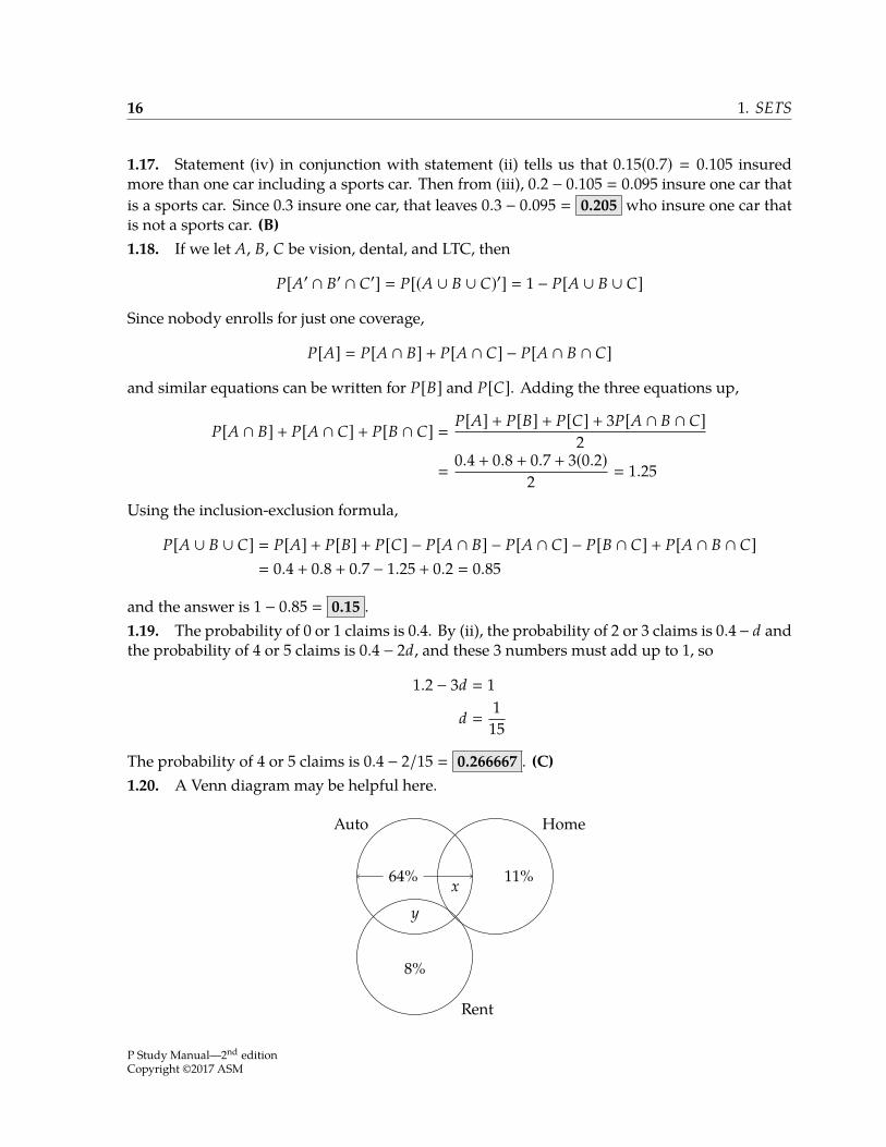
1.20. [Sample:128] An insurance agent offers his clients auto insurance, homeowners insuranceand renters insurance. The purchase of homeowners insurance and the purchase of rentersinsurance are mutually exclusive. The profile of the agent’s clients is as follows:
(i) 17% of the clients have none of these three products.(ii) 64% of the clients have auto insurance.(iii) Twice as many of the clients have homeowners insurance as have renters insurance.(iv) 35% of the clients have two of these three products.(v) 11% of the clients have homeowners insurance, but not auto insurance.
Calculate the percentage of the agent’s clients that have both auto and renters insurance.
(A) 7% (B) 10% (C) 16% (D) 25% (E) 28%
1.21. [Sample:134] A mattress store sells only king, queen and twin-size mattresses. Salesrecords at the store indicate that one-fourth as many queen-size mattresses are sold as kingand twin-size mattresses combined. Records also indicate that three times as many king-sizemattresses are sold as twin-size mattresses.
Calculate the probability that the next mattress sold is either king or queen-size.
(A) 0.12 (B) 0.15 (C) 0.80 (D) 0.85 (E) 0.95
1.22. [Sample:143] The probability that amember of a certain class of homeownerswith liabilityand property coverage will file a liability claim is 0.04, and the probability that a member of thisclass will file a property claim is 0.10. The probability that a member of this class will file aliability claim but not a property claim is 0.01.
Calculate the probability that a randomly selected member of this class of homeowners willnot file a claim of either type.
(A) 0.850 (B) 0.860 (C) 0.864 (D) 0.870 (E) 0.890
P Study Manual—2nd editionCopyright ©2017 ASM
Exercises continue on the next page . . .
EXERCISES FOR LESSON 1 11
1.23. [Sample:146] A survey of 100 TV watchers revealed that over the last year:
(i) 34 watched CBS.(ii) 15 watched NBC.(iii) 10 watched ABC.(iv) 7 watched CBS and NBC.(v) 6 watched CBS and ABC.(vi) 5 watched NBC and ABC.(vii) 4 watched CBS, NBC, and ABC.(viii) 18 watched HGTV and of these, none watched CBS, NBC, or ABC.
Calculate how many of the 100 TV watchers did not watch any of the four channels (CBS,NBC, ABC or HGTV).
(A) 1 (B) 37 (C) 45 (D) 55 (E) 82
1.24. [Sample:179] This year, a medical insurance policyholder has probability 0.70 of havingno emergency room visits, 0.85 of having no hospital stays, and 0.61 of having neither emergencyroom visits nor hospital stays.
Calculate the probability that the policyholder has at least one emergency room visit and atleast one hospital stay this year.
(A) 0.045 (B) 0.060 (C) 0.390 (D) 0.667 (E) 0.840
1.25. [Sample:198] In a certain group of cancer patients, each patient’s cancer is classified inexactly one of the following five stages: stage 0, stage 1, stage 2, stage 3, or stage 4.
i) 75% of the patients in the group have stage 2 or lower.ii) 80% of the patients in the group have stage 1 or higher.iii) 80% of the patients in the group have stage 0, 1, 3, or 4.
One patient from the group is randomly selected.Calculate the probability that the selected patient’s cancer is stage 1.
(A) 0.20 (B) 0.25 (C) 0.35 (D) 0.48 (E) 0.65
P Study Manual—2nd editionCopyright ©2017 ASM
Exercises continue on the next page . . .
12 1. SETS
1.26. [Sample:207] A policyholder purchases automobile insurance for two years. Define thefollowing events:
F = the policyholder has exactly one accident in year one.G = the policyholder has one or more accidents in year two.
Define the following events:
i) The policyholder has exactly one accident in year one and has more than one accident inyear two.
ii) The policyholder has at least two accidents during the two-year period.iii) The policyholder has exactly one accident in year one and has at least one accident in year
two.iv) The policyholder has exactly one accident in year one and has a total of two or more
accidents in the two-year period.v) The policyholder has exactly one accident in year one and has more accidents in year two
than in year one.
Determine the number of events from the above list of five that are the same as F ∩ G.(A) None(B) Exactly one(C) Exactly two(D) Exactly three(E) All
1.27. [F01:1,Sample:4] An urn contains 10 balls: 4 red and 6 blue. A second urn contains 16red balls and an unknown number of blue balls. A single ball is drawn from each urn. Theprobability that both balls are the same color is 0.44.
Calculate the number of blue balls in the second urn.
(A) 4 (B) 20 (C) 24 (D) 44 (E) 64
1.28. [S01:31,Sample:15] An insurer offers a health plan to the employees of a large company.As part of this plan, the individual employees may choose exactly two of the supplementarycoverages A, B, and C, or they may choose no supplementary coverage. The proportions of the
company’s employees that choose coverages A, B, and C are 14 ,
13 , and
512 ,respectively.
Determine the probability that a randomly chosen employee will choose no supplementarycoverage.
(A) 0 (B) 47144 (C) 1
2 (D) 97144 (E) 7
91.29. The probability of event U is 0.8 and the probability of event V is 0.4.
What is the lowest possible probability of the event U ∩ V?
P Study Manual—2nd editionCopyright ©2017 ASM
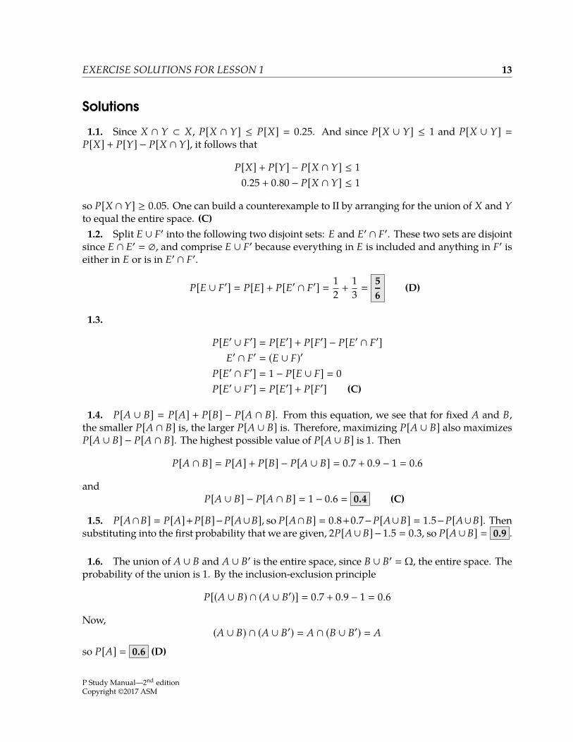
EXERCISE SOLUTIONS FOR LESSON 1 13
Solutions
1.1. Since X ∩ Y ⊂ X, P[X ∩ Y] ≤ P[X] 0.25. And since P[X ∪ Y] ≤ 1 and P[X ∪ Y] P[X] + P[Y] − P[X ∩ Y], it follows that
P[X] + P[Y] − P[X ∩ Y] ≤ 10.25 + 0.80 − P[X ∩ Y] ≤ 1
so P[X ∩Y] ≥ 0.05. One can build a counterexample to II by arranging for the union of X and Yto equal the entire space. (C)1.2. Split E ∪ F′ into the following two disjoint sets: E and E′ ∩ F′. These two sets are disjoint
since E ∩ E′ , and comprise E ∪ F′ because everything in E is included and anything in F′ iseither in E or is in E′ ∩ F′.
P[E ∪ F′] P[E] + P[E′ ∩ F′] 12 +
13
56
(D)
1.3.
P[E′ ∪ F′] P[E′] + P[F′] − P[E′ ∩ F′]E′ ∩ F′ (E ∪ F)′
P[E′ ∩ F′] 1 − P[E ∪ F] 0P[E′ ∪ F′] P[E′] + P[F′] (C)
1.4. P[A ∪ B] P[A] + P[B] − P[A ∩ B]. From this equation, we see that for fixed A and B,the smaller P[A ∩ B] is, the larger P[A ∪ B] is. Therefore, maximizing P[A ∪ B] also maximizesP[A ∪ B] − P[A ∩ B]. The highest possible value of P[A ∪ B] is 1. Then
P[A ∩ B] P[A] + P[B] − P[A ∪ B] 0.7 + 0.9 − 1 0.6
andP[A ∪ B] − P[A ∩ B] 1 − 0.6 0.4 (C)
1.5. P[A∩B] P[A]+P[B]−P[A∪B], so P[A∩B] 0.8+0.7−P[A∪B] 1.5−P[A∪B]. Thensubstituting into the first probability that we are given, 2P[A∪B] − 1.5 0.3, so P[A∪B] 0.9 .
1.6. The union of A ∪ B and A ∪ B′ is the entire space, since B ∪ B′ Ω, the entire space. Theprobability of the union is 1. By the inclusion-exclusion principle
P[(A ∪ B) ∩ (A ∪ B′)] 0.7 + 0.9 − 1 0.6
Now,(A ∪ B) ∩ (A ∪ B′) A ∩ (B ∪ B′) A
so P[A] 0.6 (D)
P Study Manual—2nd editionCopyright ©2017 ASM
14 1. SETS
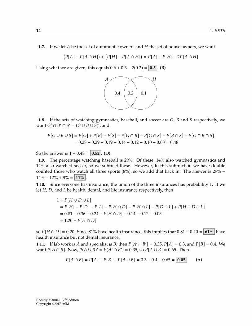
1.7. If we let A be the set of automobile owners and H the set of house owners, we want(P[A] − P[A ∩ H]) + (
P[H] − P[A ∩ H]) P[A] + P[H] − 2P[A ∩ H]
Using what we are given, this equals 0.6 + 0.3 − 2(0.2) 0.5 . (B)
0.4 0.10.2
A H
1.8. If the sets of watching gymnastics, baseball, and soccer are G, B and S respectively, wewant G′ ∩ B′ ∩ S′ (G ∪ B ∪ S)′, and
P[G ∪ B ∪ S] P[G] + P[B] + P[S] − P[G ∩ B] − P[G ∩ S] − P[B ∩ S] + P[G ∩ B ∩ S] 0.28 + 0.29 + 0.19 − 0.14 − 0.12 − 0.10 + 0.08 0.48
So the answer is 1 − 0.48 0.52 . (D)1.9. The percentage watching baseball is 29%. Of these, 14% also watched gymnastics and
12% also watched soccer, so we subtract these. However, in this subtraction we have doublecounted those who watch all three sports (8%), so we add that back in. The answer is 29% −14% − 12% + 8% 11% .1.10. Since everyone has insurance, the union of the three insurances has probability 1. If welet H, D, and L be health, dental, and life insurance respectively, then
1 P[H ∪ D ∪ L] P[H] + P[D] + P[L] − P[H ∩ D] − P[H ∩ L] − P[D ∩ L] + P[H ∩ D ∩ L] 0.81 + 0.36 + 0.24 − P[H ∩ D] − 0.14 − 0.12 + 0.05 1.20 − P[H ∩ D]
so P[H ∩ D] 0.20. Since 81% have health insurance, this implies that 0.81 − 0.20 61% havehealth insurance but not dental insurance.1.11. If lab work is A and specialist is B, then P[A′ ∩ B′] 0.35, P[A] 0.3, and P[B] 0.4. Wewant P[A ∩ B]. Now, P(A ∪ B)′ P(A′ ∩ B′) 0.35, so P[A ∪ B] 0.65. Then
P[A ∩ B] P[A] + P[B] − P[A ∪ B] 0.3 + 0.4 − 0.65 0.05 (A)
P Study Manual—2nd editionCopyright ©2017 ASM
EXERCISE SOLUTIONS FOR LESSON 1 15
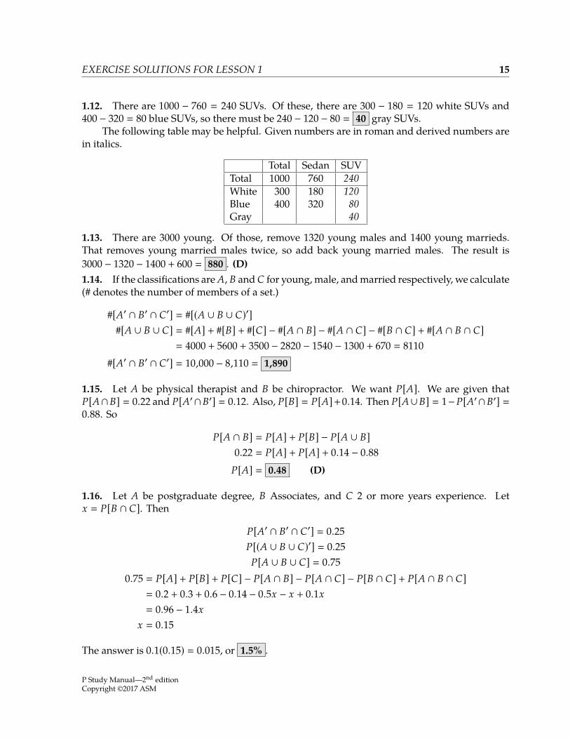
1.12. There are 1000 − 760 240 SUVs. Of these, there are 300 − 180 120 white SUVs and400 − 320 80 blue SUVs, so there must be 240 − 120 − 80 40 gray SUVs.
The following table may be helpful. Given numbers are in roman and derived numbers arein italics.
Total Sedan SUVTotal 1000 760 240White 300 180 120Blue 400 320 80Gray 40
1.13. There are 3000 young. Of those, remove 1320 young males and 1400 young marrieds.That removes young married males twice, so add back young married males. The result is3000 − 1320 − 1400 + 600 880 . (D)1.14. If the classifications are A, B and C for young, male, andmarried respectively, we calculate(# denotes the number of members of a set.)
#[A′ ∩ B′ ∩ C′] #[(A ∪ B ∪ C)′]#[A ∪ B ∪ C] #[A] + #[B] + #[C] − #[A ∩ B] − #[A ∩ C] − #[B ∩ C] + #[A ∩ B ∩ C]
4000 + 5600 + 3500 − 2820 − 1540 − 1300 + 670 8110#[A′ ∩ B′ ∩ C′] 10,000 − 8,110 1,890
1.15. Let A be physical therapist and B be chiropractor. We want P[A]. We are given thatP[A∩B] 0.22 and P[A′∩B′] 0.12. Also, P[B] P[A]+0.14. Then P[A∪B] 1−P[A′∩B′] 0.88. So
P[A ∩ B] P[A] + P[B] − P[A ∪ B]0.22 P[A] + P[A] + 0.14 − 0.88
P[A] 0.48 (D)
1.16. Let A be postgraduate degree, B Associates, and C 2 or more years experience. Letx P[B ∩ C]. Then
P[A′ ∩ B′ ∩ C′] 0.25P[(A ∪ B ∪ C)′] 0.25P[A ∪ B ∪ C] 0.75
0.75 P[A] + P[B] + P[C] − P[A ∩ B] − P[A ∩ C] − P[B ∩ C] + P[A ∩ B ∩ C] 0.2 + 0.3 + 0.6 − 0.14 − 0.5x − x + 0.1x 0.96 − 1.4x
x 0.15
The answer is 0.1(0.15) 0.015, or 1.5% .
P Study Manual—2nd editionCopyright ©2017 ASM
16 1. SETS
1.17. Statement (iv) in conjunction with statement (ii) tells us that 0.15(0.7) 0.105 insuredmore than one car including a sports car. Then from (iii), 0.2 − 0.105 0.095 insure one car thatis a sports car. Since 0.3 insure one car, that leaves 0.3 − 0.095 0.205 who insure one car thatis not a sports car. (B)1.18. If we let A, B, C be vision, dental, and LTC, then
P[A′ ∩ B′ ∩ C′] P[(A ∪ B ∪ C)′] 1 − P[A ∪ B ∪ C]Since nobody enrolls for just one coverage,
P[A] P[A ∩ B] + P[A ∩ C] − P[A ∩ B ∩ C]and similar equations can be written for P[B] and P[C]. Adding the three equations up,
P[A ∩ B] + P[A ∩ C] + P[B ∩ C] P[A] + P[B] + P[C] + 3P[A ∩ B ∩ C]2
0.4 + 0.8 + 0.7 + 3(0.2)
2 1.25
Using the inclusion-exclusion formula,
P[A ∪ B ∪ C] P[A] + P[B] + P[C] − P[A ∩ B] − P[A ∩ C] − P[B ∩ C] + P[A ∩ B ∩ C] 0.4 + 0.8 + 0.7 − 1.25 + 0.2 0.85
and the answer is 1 − 0.85 0.15 .1.19. The probability of 0 or 1 claims is 0.4. By (ii), the probability of 2 or 3 claims is 0.4− d andthe probability of 4 or 5 claims is 0.4 − 2d, and these 3 numbers must add up to 1, so
1.2 − 3d 1
d 115
The probability of 4 or 5 claims is 0.4 − 2/15 0.266667 . (C)1.20. A Venn diagram may be helpful here.
64%x
11%
8%
y
Auto Home
Rent
P Study Manual—2nd editionCopyright ©2017 ASM
EXERCISE SOLUTIONS FOR LESSON 1 17
Let x be the proportion with both auto and home and y the proportion with both auto andrenters. We are given that 17% have no product, so 83% have at least one product. 64% haveauto and 11% have homeowners but not auto, so that leaves 83% − 64% − 11% 8% who haveonly renters insurance. Now we can set up two equations in x and y. From (iv), x + y 0.35.From (iii), 0.11 + x 2(0.08 + y). Solving,
0.11 + (0.35 − y) 0.16 + 2y0.46 − 0.16 3y
y 0.10 (B)
1.21. We’ll use K, Q, and T for the three events king-size, queen-size, and twin-size mattresses.We’re given P[K]+ P[T] 4P[Q] and P[K] 3P[T], and the three events are mutually exclusiveand exhaustive so their probabilities must add up to 1, P[K] + P[T] + P[Q] 1. We have threeequations in three unknowns. Let’s solve for P[T] and then use the complement.
3P[T] + P[T] 4P[Q] 4(1 − 4P[T])4P[T] 4 − 16P[T]
P[T] 0.2
and the answer is 1 − 0.2 0.8 . (C)1.22. We want to calculate the probability of filing some claim, or the union of those filingproperty and liability claims, because then we can calculate the probability of the complementof this set, those who file no claim. To calculate the probability of filing some claim, we need theprobability of filing both types of claim.
The probability that a member will file a liability claim is 0.04, and of these 0.01 do notfile a property claim so 0.03 do file both claims. The probability of the union of those who fileliability and property claims is the sum of the probabilities of filing either type of claim, minusthe probability of filing both types of claim, or 0.04 + 0.10− 0.03 0.11, so the probability of notfiling either type of claim is 1 − 0.11 0.89 . (E)1.23. First let’s calculate how many did not watch CBS, NBC, or ABC. As usual, we add up theones who watched one, minus the ones who watched two, plus the ones who watched three:
34 + 15 + 10 − 7 − 6 − 5 + 4 45
An additional 18 watched HGTV for a total of 63 who watched something. 100 − 63 37watched nothing. (B)1.24. Let A be the event of an emergency room visit and B the event of a hospital stay. We haveP[A] 1 − 0.7 0.3 and P[B] 1 − 0.85 0.15. Also P[A ∪ B] 1 − 0.61 0.39. Then theprobability we want is
P[A ∩ B] P[A] + P[B] − P[A ∪ B] 0.3 + 0.15 − 0.39 0.06 (B)
P Study Manual—2nd editionCopyright ©2017 ASM
18 1. SETS
1.25. From ii), the probability of stage 0 is 20%. From iii), the probability of stage 2 is 20%. Fromi), the probability of stage 0, 1, or 2 is 75%. So the probability of stage 1 is 0.75 − 2(0.2) 0.35 .(C)1.26. F ∩ G is the event of exactly one accident in year one and at least one in year two.i) This event is not the same since it excludes the event of one in year one and one in year
two.#ii) This event is not the same since it includes two in year one and none in year two, among
others.#iii) This event is the same.!iv) This event is the same, since to have two or more accidents total, there must be one or more
accidents in year two.!
v) This event is not the same since it excludes having one in year one and one in year two.#(C)1.27. Let x be the number of blue balls in the second urn. Then the probability that both ballsare red is 0.4(16)/(16 + x) and the probability that both balls are blue is 0.6x/(16 + x). The sumof these two expressions is 0.44, so
6.4 + 0.6x16 + x
0.44
6.4 + 0.6x 7.04 + 0.44x0.16x 0.64
x 4 (A)
1.28. P[A] P[A∩B]+P[A∩C], since the only way to have coverage A is in combination withexactly one of B and C. Similarly P[B] P[B ∩ A] + P[B ∩ C] and P[C] P[C ∩ A] + P[C ∩ B].Adding up the three equalities, we get
P[A] + P[B] + P[C] 2(P[A ∩ B] + P[A ∩ C] + P[B ∩ C]) 1
4 +13 +
512 1
so the sum of the probabilities of two coverages is 0.5. But the only alternative to two coveragesis no coverage, so the probability of no coverage is 1 − 0.5 0.5 . (C)1.29. The probability of U ∪ V cannot be more than 1, and
P[U ∩ V] P[U] + P[V] − P[U ∪ V] 0.8 + 0.4 − P[U ∪ V]Using themaximal value of P[U∪V], we get theminimal value of P[U∩V] ≥ 0.8+0.4−1 0.2 .
P Study Manual—2nd editionCopyright ©2017 ASM
Practice Exam 1
1. Six actuarial students are all equally likely to pass Exam P. Their probabilities of passingare mutually independent. The probability all 6 pass is 0.24.
Calculate the variance of the number of students who pass.
(A) 0.98 (B) 1.00 (C) 1.02 (D) 1.04 (E) 1.06
2. The number of claims in a year, N , on an insurance policy has a Poisson distribution withmean 0.25. The numbers of claims in different years are mutually independent.
Calculate the probability of 3 or more claims over a period of 2 years.
(A) 0.001 (B) 0.010 (C) 0.012 (D) 0.014 (E) 0.016
3. Claim sizes on an insurance policy have the following distribution:
F(x)
0, x ≤ 00.0002x 0 < x < 10000.4, x 10001 − 0.6e−(x−1000)/2000 x > 1000
Calculate expected claim size.
(A) 1500 (B) 1700 (C) 1900 (D) 2100 (E) 2300
4. Anactuary analyzesweekly sales of automobile insurance, X, andhomeowners insurance,Y. The analysis reveals that Var(X) 2500, Var(Y) 900, and Var(X + Y) 3100.
Calculate the correlation of X and Y.
(A) −0.2 (B) −0.1 (C) 0 (D) 0.1 (E) 0.2
5. Adevice runs until either of two components fail, at which point the device stops running.The joint distribution function of the lifetimes of the two components is F(s , t). The joint densityfunction is nonzero only when 0 < s < 1 and 0 < t < 1.
Determine which of the following represents the probability that the device fails during thefirst half hour of operation.(A) F(0.5, 0.5)(B) 1 − F(0.5, 0.5)(C) F(0.5, 1) + F(1, 0.5)(D) F(0.5, 1) + F(1, 0.5) − F(0.5, 0.5)(E) F(0.5, 1) + F(1, 0.5) − F(1, 1)
P Study Manual—2nd editionCopyright ©2017 ASM
425 Exam questions continue on the next page . . .
426 PRACTICE EXAM 1
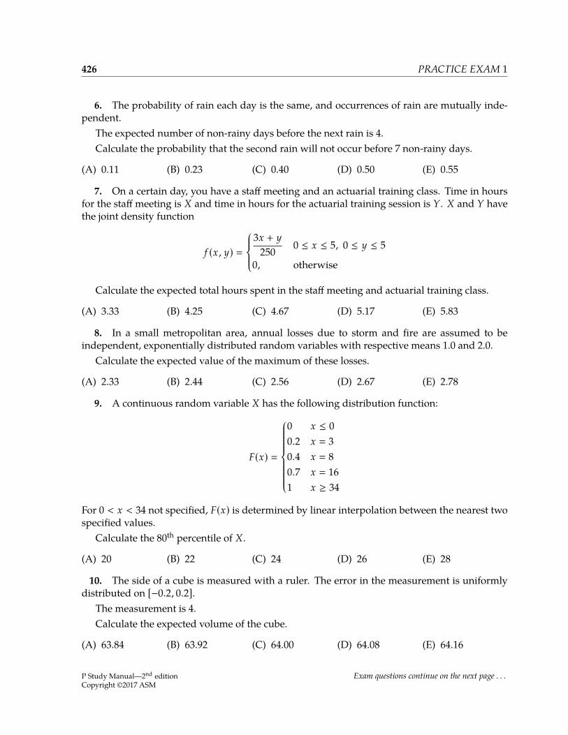
6. The probability of rain each day is the same, and occurrences of rain are mutually inde-pendent.
The expected number of non-rainy days before the next rain is 4.Calculate the probability that the second rain will not occur before 7 non-rainy days.
(A) 0.11 (B) 0.23 (C) 0.40 (D) 0.50 (E) 0.55
7. On a certain day, you have a staff meeting and an actuarial training class. Time in hoursfor the staff meeting is X and time in hours for the actuarial training session is Y. X and Y havethe joint density function
f (x , y)
3x + y250 0 ≤ x ≤ 5, 0 ≤ y ≤ 5
0, otherwise
Calculate the expected total hours spent in the staff meeting and actuarial training class.
(A) 3.33 (B) 4.25 (C) 4.67 (D) 5.17 (E) 5.83
8. In a small metropolitan area, annual losses due to storm and fire are assumed to beindependent, exponentially distributed random variables with respective means 1.0 and 2.0.
Calculate the expected value of the maximum of these losses.
(A) 2.33 (B) 2.44 (C) 2.56 (D) 2.67 (E) 2.78
9. A continuous random variable X has the following distribution function:
F(x)
0 x ≤ 00.2 x 30.4 x 80.7 x 161 x ≥ 34
For 0 < x < 34 not specified, F(x) is determined by linear interpolation between the nearest twospecified values.
Calculate the 80th percentile of X.
(A) 20 (B) 22 (C) 24 (D) 26 (E) 28
10. The side of a cube is measured with a ruler. The error in the measurement is uniformlydistributed on [−0.2, 0.2].
The measurement is 4.Calculate the expected volume of the cube.
(A) 63.84 (B) 63.92 (C) 64.00 (D) 64.08 (E) 64.16
P Study Manual—2nd editionCopyright ©2017 ASM
Exam questions continue on the next page . . .
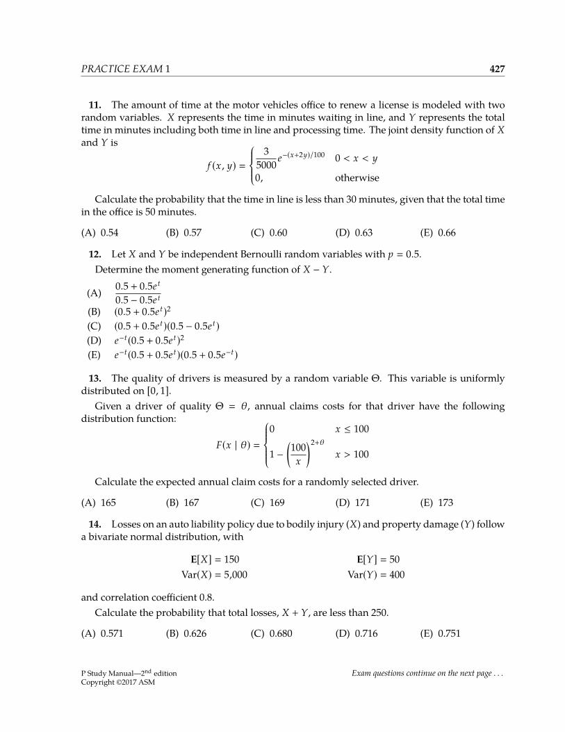
PRACTICE EXAM 1 427
11. The amount of time at the motor vehicles office to renew a license is modeled with tworandom variables. X represents the time in minutes waiting in line, and Y represents the totaltime in minutes including both time in line and processing time. The joint density function of Xand Y is
f (x , y)
35000 e−(x+2y)/100 0 < x < y
0, otherwise
Calculate the probability that the time in line is less than 30 minutes, given that the total timein the office is 50 minutes.
(A) 0.54 (B) 0.57 (C) 0.60 (D) 0.63 (E) 0.66
12. Let X and Y be independent Bernoulli random variables with p 0.5.Determine the moment generating function of X − Y.
(A) 0.5 + 0.5e t
0.5 − 0.5e t
(B) (0.5 + 0.5e t)2(C) (0.5 + 0.5e t)(0.5 − 0.5e t)(D) e−t(0.5 + 0.5e t)2(E) e−t(0.5 + 0.5e t)(0.5 + 0.5e−t)
13. The quality of drivers is measured by a random variable Θ. This variable is uniformlydistributed on [0, 1].
Given a driver of quality Θ θ, annual claims costs for that driver have the followingdistribution function:
F(x | θ)
0 x ≤ 100
1 −(100x
)2+θ
x > 100
Calculate the expected annual claim costs for a randomly selected driver.
(A) 165 (B) 167 (C) 169 (D) 171 (E) 173
14. Losses on an auto liability policy due to bodily injury (X) and property damage (Y) followa bivariate normal distribution, with
E[X] 150 E[Y] 50Var(X) 5,000 Var(Y) 400
and correlation coefficient 0.8.Calculate the probability that total losses, X + Y, are less than 250.
(A) 0.571 (B) 0.626 (C) 0.680 (D) 0.716 (E) 0.751
P Study Manual—2nd editionCopyright ©2017 ASM
Exam questions continue on the next page . . .
428 PRACTICE EXAM 1
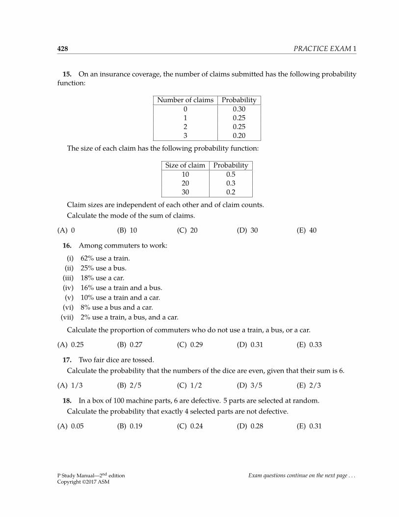
15. On an insurance coverage, the number of claims submitted has the following probabilityfunction:
Number of claims Probability0 0.301 0.252 0.253 0.20
The size of each claim has the following probability function:
Size of claim Probability10 0.520 0.330 0.2
Claim sizes are independent of each other and of claim counts.Calculate the mode of the sum of claims.
(A) 0 (B) 10 (C) 20 (D) 30 (E) 40
16. Among commuters to work:
(i) 62% use a train.(ii) 25% use a bus.(iii) 18% use a car.(iv) 16% use a train and a bus.(v) 10% use a train and a car.(vi) 8% use a bus and a car.(vii) 2% use a train, a bus, and a car.
Calculate the proportion of commuters who do not use a train, a bus, or a car.
(A) 0.25 (B) 0.27 (C) 0.29 (D) 0.31 (E) 0.33
17. Two fair dice are tossed.Calculate the probability that the numbers of the dice are even, given that their sum is 6.
(A) 1/3 (B) 2/5 (C) 1/2 (D) 3/5 (E) 2/3
18. In a box of 100 machine parts, 6 are defective. 5 parts are selected at random.Calculate the probability that exactly 4 selected parts are not defective.
(A) 0.05 (B) 0.19 (C) 0.24 (D) 0.28 (E) 0.31
P Study Manual—2nd editionCopyright ©2017 ASM
Exam questions continue on the next page . . .
PRACTICE EXAM 1 429
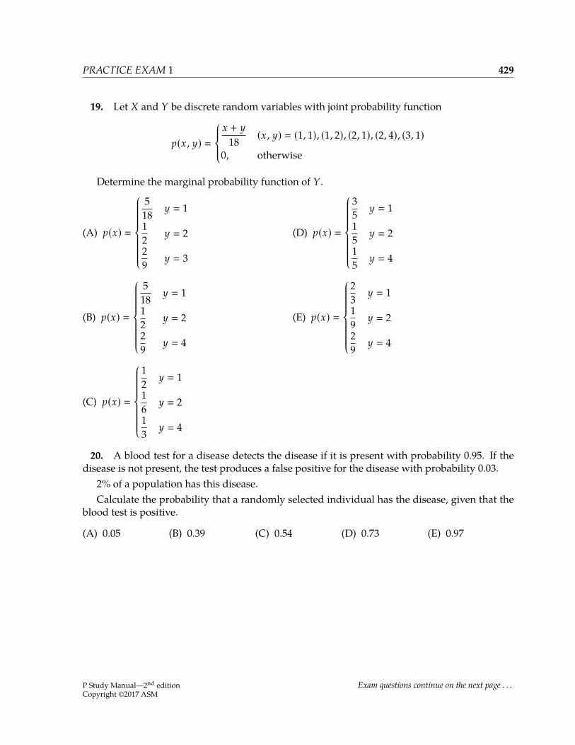
19. Let X and Y be discrete random variables with joint probability function
p(x , y)
x + y18 (x , y) (1, 1), (1, 2), (2, 1), (2, 4), (3, 1)
0, otherwise
Determine the marginal probability function of Y.
(A) p(x)
518 y 1
12 y 2
29 y 3
(D) p(x)
35 y 1
15 y 2
15 y 4
(B) p(x)
518 y 1
12 y 2
29 y 4
(E) p(x)
23 y 1
19 y 2
29 y 4
(C) p(x)
12 y 1
16 y 2
13 y 4
20. A blood test for a disease detects the disease if it is present with probability 0.95. If thedisease is not present, the test produces a false positive for the disease with probability 0.03.
2% of a population has this disease.Calculate the probability that a randomly selected individual has the disease, given that the
blood test is positive.
(A) 0.05 (B) 0.39 (C) 0.54 (D) 0.73 (E) 0.97
P Study Manual—2nd editionCopyright ©2017 ASM
Exam questions continue on the next page . . .
430 PRACTICE EXAM 1
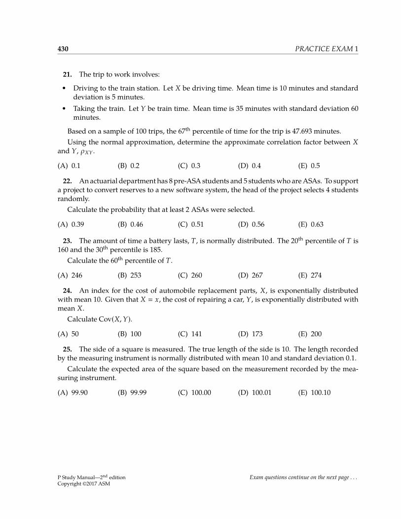
21. The trip to work involves:
• Driving to the train station. Let X be driving time. Mean time is 10 minutes and standarddeviation is 5 minutes.
• Taking the train. Let Y be train time. Mean time is 35 minutes with standard deviation 60minutes.
Based on a sample of 100 trips, the 67th percentile of time for the trip is 47.693 minutes.Using the normal approximation, determine the approximate correlation factor between X
and Y, ρXY .
(A) 0.1 (B) 0.2 (C) 0.3 (D) 0.4 (E) 0.5
22. Anactuarial department has 8 pre-ASA students and 5 studentswho areASAs. To supporta project to convert reserves to a new software system, the head of the project selects 4 studentsrandomly.
Calculate the probability that at least 2 ASAs were selected.
(A) 0.39 (B) 0.46 (C) 0.51 (D) 0.56 (E) 0.63
23. The amount of time a battery lasts, T, is normally distributed. The 20th percentile of T is160 and the 30th percentile is 185.
Calculate the 60th percentile of T.
(A) 246 (B) 253 (C) 260 (D) 267 (E) 274
24. An index for the cost of automobile replacement parts, X, is exponentially distributedwith mean 10. Given that X x, the cost of repairing a car, Y, is exponentially distributed withmean X.
Calculate Cov(X,Y).(A) 50 (B) 100 (C) 141 (D) 173 (E) 200
25. The side of a square is measured. The true length of the side is 10. The length recordedby the measuring instrument is normally distributed with mean 10 and standard deviation 0.1.
Calculate the expected area of the square based on the measurement recorded by the mea-suring instrument.
(A) 99.90 (B) 99.99 (C) 100.00 (D) 100.01 (E) 100.10
P Study Manual—2nd editionCopyright ©2017 ASM
Exam questions continue on the next page . . .
PRACTICE EXAM 1 431
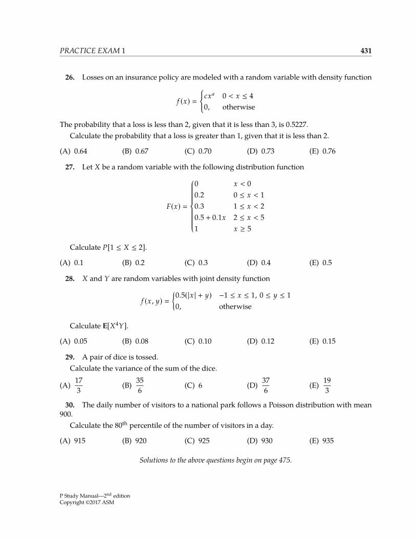
26. Losses on an insurance policy are modeled with a random variable with density function
f (x)
cxa 0 < x ≤ 40, otherwise
The probability that a loss is less than 2, given that it is less than 3, is 0.5227.Calculate the probability that a loss is greater than 1, given that it is less than 2.
(A) 0.64 (B) 0.67 (C) 0.70 (D) 0.73 (E) 0.76
27. Let X be a random variable with the following distribution function
F(x)
0 x < 00.2 0 ≤ x < 10.3 1 ≤ x < 20.5 + 0.1x 2 ≤ x < 51 x ≥ 5
Calculate P[1 ≤ X ≤ 2].(A) 0.1 (B) 0.2 (C) 0.3 (D) 0.4 (E) 0.5
28. X and Y are random variables with joint density function
f (x , y) 0.5(|x | + y) −1 ≤ x ≤ 1, 0 ≤ y ≤ 10, otherwise
Calculate E[X4Y].(A) 0.05 (B) 0.08 (C) 0.10 (D) 0.12 (E) 0.15
29. A pair of dice is tossed.Calculate the variance of the sum of the dice.
(A) 173 (B) 35
6 (C) 6 (D) 376 (E) 19
3
30. The daily number of visitors to a national park follows a Poisson distribution with mean900.
Calculate the 80th percentile of the number of visitors in a day.
(A) 915 (B) 920 (C) 925 (D) 930 (E) 935
Solutions to the above questions begin on page 475.
P Study Manual—2nd editionCopyright ©2017 ASM
432 PRACTICE EXAM 1
P Study Manual—2nd editionCopyright ©2017 ASM
Appendix A. Solutions to the Practice Exams
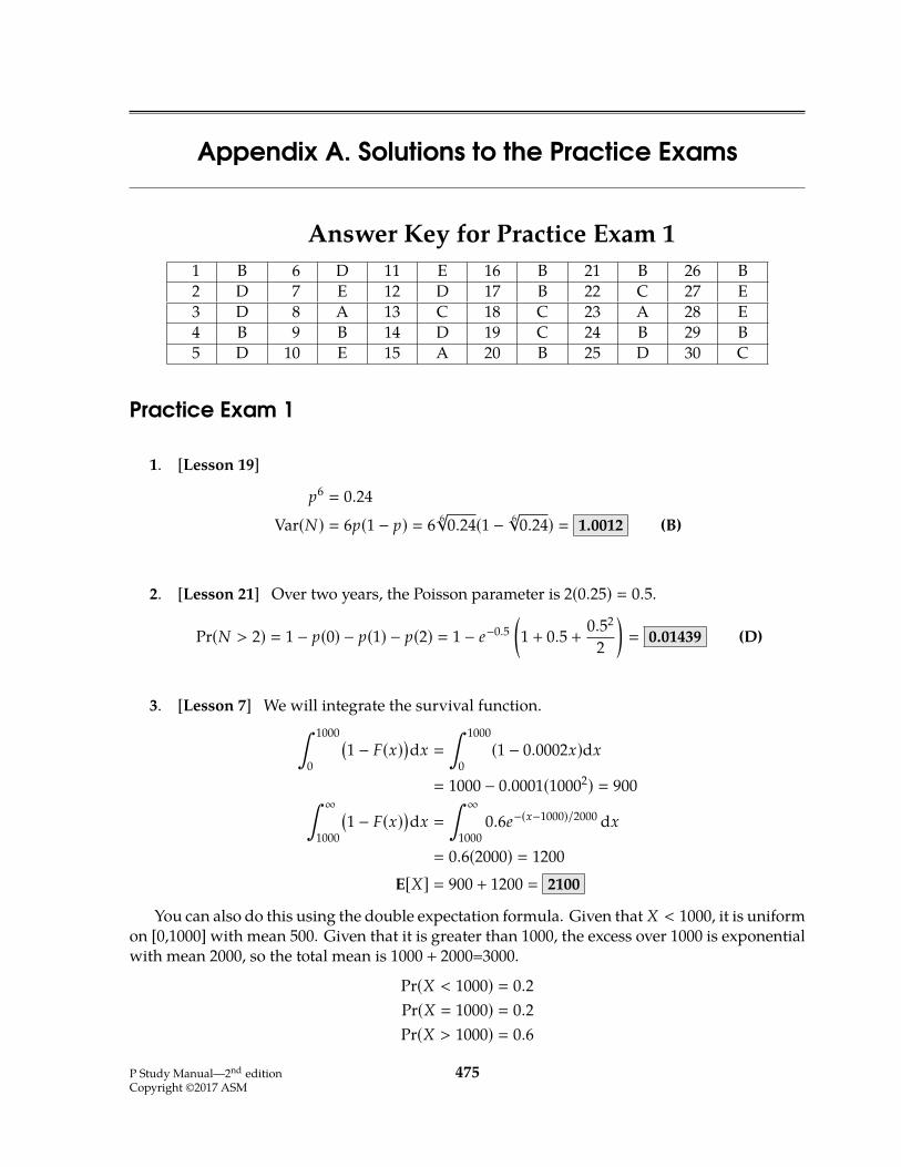
Answer Key for Practice Exam 11 B 6 D 11 E 16 B 21 B 26 B2 D 7 E 12 D 17 B 22 C 27 E3 D 8 A 13 C 18 C 23 A 28 E4 B 9 B 14 D 19 C 24 B 29 B5 D 10 E 15 A 20 B 25 D 30 C
Practice Exam 1
1. [Lesson 19]
p6 0.24
Var(N) 6p(1 − p) 6 6√0.24(1 − 6√0.24) 1.0012 (B)
2. [Lesson 21] Over two years, the Poisson parameter is 2(0.25) 0.5.
Pr(N > 2) 1 − p(0) − p(1) − p(2) 1 − e−0.5(1 + 0.5 +
0.52
2
) 0.01439 (D)
3. [Lesson 7] We will integrate the survival function.∫ 1000
0
(1 − F(x))dx
∫ 1000
0(1 − 0.0002x)dx
1000 − 0.0001(10002) 900∫ ∞
1000
(1 − F(x))dx
∫ ∞
10000.6e−(x−1000)/2000 dx
0.6(2000) 1200E[X] 900 + 1200 2100
You can also do this using the double expectation formula. Given that X < 1000, it is uniformon [0,1000] with mean 500. Given that it is greater than 1000, the excess over 1000 is exponentialwith mean 2000, so the total mean is 1000 + 2000=3000.
Pr(X < 1000) 0.2Pr(X 1000) 0.2Pr(X > 1000) 0.6
P Study Manual—2nd editionCopyright ©2017 ASM
475
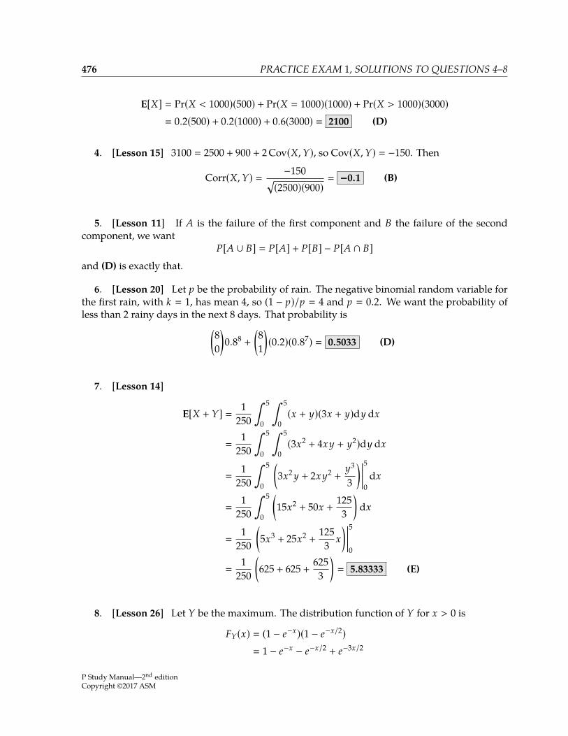
476 PRACTICE EXAM 1, SOLUTIONS TO QUESTIONS 4–8
E[X] Pr(X < 1000)(500) + Pr(X 1000)(1000) + Pr(X > 1000)(3000) 0.2(500) + 0.2(1000) + 0.6(3000) 2100 (D)
4. [Lesson 15] 3100 2500 + 900 + 2 Cov(X,Y), so Cov(X,Y) −150. Then
Corr(X,Y) −150√(2500)(900)
−0.1 (B)
5. [Lesson 11] If A is the failure of the first component and B the failure of the secondcomponent, we want
P[A ∪ B] P[A] + P[B] − P[A ∩ B]and (D) is exactly that.
6. [Lesson 20] Let p be the probability of rain. The negative binomial random variable forthe first rain, with k 1, has mean 4, so (1 − p)/p 4 and p 0.2. We want the probability ofless than 2 rainy days in the next 8 days. That probability is(
80
)0.88
+
(81
)(0.2)(0.87) 0.5033 (D)
7. [Lesson 14]
E[X + Y] 1250
∫ 5
0
∫ 5
0(x + y)(3x + y)dy dx
1
250
∫ 5
0
∫ 5
0(3x2
+ 4x y + y2)dy dx
1
250
∫ 5
0
(3x2 y + 2x y2
+y3
3
)5
0dx
1
250
∫ 5
0
(15x2
+ 50x +125
3
)dx
1
250
(5x3
+ 25x2+
1253 x
)5
0
1
250
(625 + 625 +
6253
) 5.83333 (E)
8. [Lesson 26] Let Y be the maximum. The distribution function of Y for x > 0 is
FY(x) (1 − e−x)(1 − e−x/2) 1 − e−x − e−x/2
+ e−3x/2
P Study Manual—2nd editionCopyright ©2017 ASM
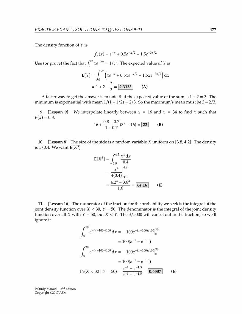
PRACTICE EXAM 1, SOLUTIONS TO QUESTIONS 9–11 477
The density function of Y is
fY(x) e−x+ 0.5e−x/2 − 1.5e−3x/2
Use (or prove) the fact that∫ ∞
0 xe−cx 1/c2. The expected value of Y is
E[Y] ∫ ∞
0
(xe−x
+ 0.5xe−x/2 − 1.5xe−3x/2)
dx
1 + 2 − 23 2.3333 (A)
A faster way to get the answer is to note that the expected value of the sum is 1 + 2 3. Theminimum is exponential with mean 1/(1+ 1/2) 2/3. So the maximum’s mean must be 3− 2/3.
9. [Lesson 9] We interpolate linearly between x 16 and x 34 to find x such thatF(x) 0.8.
16 +0.8 − 0.71 − 0.7 (34 − 16) 22 (B)
10. [Lesson 8] The size of the side is a random variable X uniform on [3.8, 4.2]. The densityis 1/0.4. We want E[X3].
E[X3] ∫ 4.2
3.8
x3 dx0.4
x4
4(0.4)4.2
3.8
4.24 − 3.84
1.6 64.16 (E)
11. [Lesson 16] The numerator of the fraction for the probability we seek is the integral of thejoint density function over X < 30, Y 50. The denominator is the integral of the joint densityfunction over all X with Y 50, but X < Y. The 3/5000 will cancel out in the fraction, so we’llignore it. ∫ 50
0e−(x+100)/100 dx − 100e−(x+100)/10050
0
100(e−1 − e−1.5)∫ 30
0e−(x+100)/100 dx − 100e−(x+100)/10030
0
100(e−1 − e−1.3)
Pr(X < 30 | Y 50) e−1 − e−1.3
e−1 − e−1.5 0.6587 (E)
P Study Manual—2nd editionCopyright ©2017 ASM
478 PRACTICE EXAM 1, SOLUTIONS TO QUESTIONS 12–14
12. [Lesson 27] The probability function of X − Y isn p(n)−1 0.250 0.501 0.25
Therefore, the MGF isM(t) 0.25e−t
+ 0.5 + 0.25e t
which is the same as (D)
13. [Lesson 18] We’ll use the double expectation formula. The density function of theconditional claim costs is
f (x | θ) dF(x | θ)dx
(2 + θ)1002+θ
x3+θ
with mean
E[X | θ] ∫ ∞
100
(2 + θ)1002+θdxx2+θ
100(2 + θ)(1 + θ)
We now use the double expectation formula.
E[X] EΘ[E[X | θ]]
∫ 1
0
100(2 + θ)1 + θ
fΘ(θ)dθ
Θ follows a uniform distribution on [0, 1], so fΘ(θ) 1.
E[X] ∫ 1
0
100(2 + θ)1 + θ
dθ
100∫ 1
0
(1 +
11 + θ
)dθ
100(θ + ln(1 + θ)) 1
0
100(1 + ln 2) 169.31 (C)
14. [Lesson 24] The sum is normal with mean 150 + 50 200 and variance
5000 + 400 + 2(0.8)√(5000)(400) 7662.74
The probability this is less than 250 is
Φ
(250 − 200√
7662.74
) Φ(0.571) 0.7160 (D)
P Study Manual—2nd editionCopyright ©2017 ASM
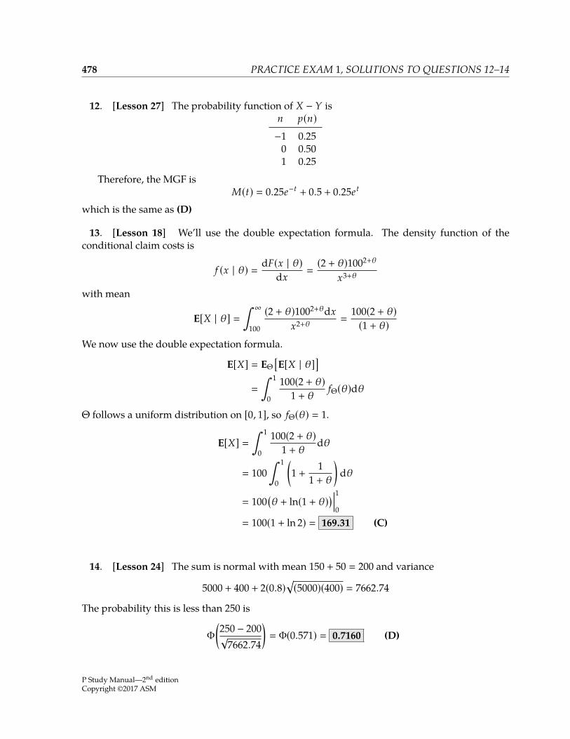
PRACTICE EXAM 1, SOLUTIONS TO QUESTIONS 15–20 479
15. [Lesson 10] Let X be total claims. We have to add up probabilities of all ways of reachingmultiples of 10.
Pr(X 0) 0.3Pr(X 10) 0.25(0.5) 0.125Pr(X 20) 0.25(0.3) + 0.25(0.52) 0.1375Pr(X 30) 0.25(0.2) + 0.25(2)(0.5)(0.3) + 0.20(0.53) 0.15
We stop here, because the probabilities already sum up to 0.7125, so the remaining probabilitiesare certainly less than 0.3, the probability of 0 . (A)
16. [Lesson 1] Let T be train, B be bus, C be car.
P[T ∪ B ∪ C] P[T] + P[B] + P[C] − P[T ∩ B] − P[T ∩ C] − P[B ∩ C] + P[T ∩ B ∩ C] 0.62 + 0.25 + 0.18 − 0.16 − 0.10 − 0.08 + 0.02 0.73
P[(T ∪ B ∪ C)′] 1 − 0.73 0.27 (B)
17. [Lesson 3] There are three ways to get 6 as a sum of two odd numbers: 1 + 5, 3 + 3, 5 + 1.There are two ways to get 6 as a sum of two even numbers: 2 + 4 and 4 + 2. Since these are allequally likely, the probability that both are even is 2/5 . (B)
18. [Lesson 2] (944) (6
1)
(1005) 0.24303 (C)
19. [Lesson 13] Pr(Y 1) is the sum of the probabilities of (1,1), (2,1), (3,1), or
1 + 1 + 2 + 1 + 3 + 118
12
We already see that (C) is the answer. Continuing, Pr(Y 2) is the probability of (1,2), or(1 + 2)/18 1/6, and Pr(Y 4) is the probability of (2,4), or (2 + 4)/18 1/3.
20. [Lesson 4] Use Bayes’ Theorem. Let D be the disease, P a positive result of the test.
P[D | P] P[P | D]P[D]P[P | D]P[D] + P[P | D′]P[D′]
(0.95)(0.02)
(0.95)(0.02) + (0.03)(0.98) 0.3926 (B)
P Study Manual—2nd editionCopyright ©2017 ASM
480 PRACTICE EXAM 1, SOLUTIONS TO QUESTIONS 21–23
21. [Lesson 25] The mean time for the trip is 10 + 35 45. Let Z X + Y and let Z be thesample mean of Z. Based on the normal approximation applied to the given information,
45 + z0.67
√Var(Z) 45 + 0.44
√Var(Z) 47.693
Var(Z) (2.6930.44
)2
37.460
The variance of the mean is the variance of the distribution divided by the size of the sample, sothe variance of Z is approximately 3746.0. Back out Cov(X,Y):
3746.0 52+ 602
+ 2 Cov(X,Y)Cov(X,Y) 3746 − 3625
2 60.50
The correlation coefficient is approximately
ρ 60.50(5)(60) 0.202 (B)
22. [Lesson 2] Total number of selections:(13
4) 715.
Ways to select 2 ASAs:(82) (5
2) 280.
Ways to select 3 ASAs:(81) (5
3) 80.
Ways to select 4 ASAs:(80) (5
4) 5.
280 + 80 + 5715 0.51049 (C)
23. [Lesson 23] For a standard normal distribution, 20th percentile is −0.842 and 30th per-centile is −0.524. Also, 60th percentile is 0.253. We have
µ − 0.842σ 160µ − 0.524σ 185
Soσ
185 − 1600.842 − 0.524 78.616
andµ + 0.253σ 185 + (0.253 + 0.524)(78.616) 246 (A)
P Study Manual—2nd editionCopyright ©2017 ASM
PRACTICE EXAM 1, SOLUTIONS TO QUESTIONS 24–27 481
24. [Lesson 22] Cov(X,Y) E[XY] − E[X]E[Y] and E[X] 10. The expected value of Y canbe calculated using the double expectation formula:
E[Y] E[E[Y | X]] E[X] 10
To calculate E[XY], use the double expectation formula.
E[XY] E[E[XY | X]] E[X2]
The second moment of an exponential is Var(X) + E[X]2, which here is 100 + 102 200. Then
Cov(X,Y) 200 − (10)(10) 100 (B)
25. [Lesson 23] We are asked for E[X2] where X is the length recorded by the measuringinstrument.
E[X2] Var(X) + E[X]2 0.12+ 102
100.01 (D)
26. [Lesson 6] Let’s solve for a.
0.5227 Pr(X < 2 | X < 3) F(2)F(3)
2a+1
3a+1
(23
) a+1
ln 0.5227 (a + 1) ln(2/3)a
ln 0.5227ln(2/3) − 1 0.6
Now we can calculate Pr(X > 1 | X < 2). We never need c, since it cancels in numerator anddenominator.
Pr(X > 1 | X < 2) Pr(1 < X < 2)Pr(X < 2)
2a+1 − 1a+1
2a+1
21.6 − 1
21.6 0.6701 (B)
27. [Lesson 5]F(2) − F(1−) 0.7 − 0.2 0.5 (E)
P Study Manual—2nd editionCopyright ©2017 ASM
482 PRACTICE EXAM 1, SOLUTIONS TO QUESTIONS 28–30
28. [Lesson 14] Notice that the density and X4Y are symmetric around x 0, so we cancalculate the required integral from x 0 to x 1 and double it.
0.5 E[X4Y] ∫ 1
0
∫ 1
00.5x4 y(x + y)dy dx
0.5∫ 1
0
∫ 1
0(x5 y + x4 y2)dy dx
0.5∫ 1
0
(x5 y2
2 +x4 y3
3
)1
0dx
0.5∫ 1
0
(x5
2 +x4
3
)dx
0.5(
112 +
115
) 0.5(0.15)
The answer is 0.15 . (E)
29. [Lesson 12] Since the dice are independent, the variance of the sum is the sum of thevariances. The variance of each die’s toss is (n2 − 1)/12 with n 6, or 35/12. The variance of thesum of two dice is 35/6 . (B)
30. [Lesson 25] It is not reasonable to calculate this exactly, so the normal approximation isused. The 80th percentile of a standard normal distribution is 0.842. The mean and variance ofnumber of visitors is 900. So the 80th percentile of number of visitors is 900+0.842
√900 925.26 .
(C)
P Study Manual—2nd editionCopyright ©2017 ASM

78- 1- 63588- 191- 29
ASM Study Manualfor SOA Exam P