Working Paper No. 595

Katherine Casey

March 2017

Snap Judgments: Voter Inferences Based on

Candidate Photos Predict Electoral Success and Politician Quality

 

 

Snap judgments:

Voter inferences based on candidate photos predict electoral success and politician quality

Katherine Casey*

30 March 2017

Abstract

Voting is fundamentally a forecasting problem: voters try to predict future performance in office based on incomplete information about candidates. Forecast inputs combine observable professional qualifications with more subjective assessments of confidence and trustworthiness. In developing countries, the amount of information available can be quite limited. This paper explores how well voters do in predicting candidate performance and quality under varying degrees and types of information. It leverages a series of lab-in-the-field experiments in a weak media environment where ballot photos are both the first and last visual impression many voters have of candidates. Inferences based on candidate photos alone predict who later wins actual elections. Further, these inferences are better at identifying trustworthy politicians (i.e. those who divert fewer public resources to personal use) than a suite of professional qualifications. Candidates with more electable faces appear to have stronger persuasion skills, which reflect advantages in both physical appearance and oral communication. Neither snap judgments based on photos nor observable characteristics distinguish politicians along concrete measures of effort.

__________________________ * Stanford University Graduate School of Business, 655 Knight Way, Stanford CA 94305, +1 650 725 2167, kecasey@stanford.edu. I thank K. Bidwell and R. Glennerster for collaboration on related projects; and M. Alsan, J. Bendor, E. Blankespoor, D. Broockman, A. Chandrasekhar, J. Fearon, S. Jha, D. Laitin, E. Miguel, M. Morten and S. Seiler for comments. I am grateful for excellent field and research assistance from A. Barnett, N. Eubank, A. Lahai, A. Mansaray, F. Momoh, O. Nabay, K. Parry, C. Sánchez-Martínez and Innovations for Poverty Action. I gratefully acknowledge funding from the Governance Initiative at J-PAL.

 

1  

Introduction

Voting is fundamentally a forecasting problem: voters try to predict future performance in office based on imperfect information about candidates. Forecast inputs include observable objective qualifications, like resume indicators of education and professional experience, as well as more intangible subjective criteria, like confidence and trustworthiness. There is further evidence that candidates derive rents from characteristics, like physical attractiveness, whose connection to productivity is questionable. Improving the accuracy of voter forecasts requires understanding how voters process the incomplete information available to them, and identifying the conditions under which their inferences distinguish high from low productivity types or merely promulgate inaccurate stereotypes.

In the developing world, this forecasting challenge is more difficult because voters have less access to mass media and political information. Moreover, the weak institutional checks on politician behavior that characterize new democracies raise the stakes for correctly identifying candidates with strong innate competencies and integrity. My empirical setting of Sierra Leone provides a compelling case in point. It is a low information environment, where ballot photos are both the first and last visual impression many voters have of candidates. Those elected are generally free from formal scrutiny: the Members of Parliament (MPs) studied here, for example, face no monitoring or reporting requirements for how they spend public funds earmarked for the development of their constituencies.

This paper presents results from a series of lab-in-the-field experiments that gauge the accuracy of voter forecasts about politician performance under different types of information in Sierra Leone. The paper makes two contributions. First, a pre-election lab shows that voter inferences based on candidate photos alone predict who later wins actual elections with accuracy greater than chance. This reproduces results from two seminal forecasting studies in the U.S. in a markedly different empirical context. Todorov et al. (2005) and Benjamin and Shapiro (2009) show that “thin slice” inferences by college students based on photos and video clips (respectively) accurately predict results of congressional and gubernatorial races (1-3). The Sierra Leone lab is distinctive in that all participants were registered voters, representative of the population of interest, and it was run in the weeks before the election, alleviating concerns about participant ex post awareness of election outcomes. The similarity of results across such distinct empirical contexts is notable in light of concerns that lab findings based on Western college students do not generalize to other populations (4), and attests to the strength of the results in the original studies, as the (non-) reproducibility of findings in social science has become an issue of significant concern (5).

The second, and main, contribution is to extend the forecasting exercise to concrete measures of performance. I test whether these same snap judgments distinguish politicians along several quality dimensions, defined by what voters in Sierra Leone say they are looking for in candidates: 77% of lab participants say they value education, honesty (53%), hard work (45%) and persuasiveness (32%) as the most important qualities of elected MPs. Analysis accordingly leverages rich data on politicians’ professional qualifications, trustworthiness in managing public funds, effort exerted holding meetings and participating in Parliament, and debating skill in advocating for greater funding to support the development of a particular sector.

My results suggest that voter inferences under highly limited information favor candidates who look less good on paper, but deliver more public goods in office. First, snap judgments based on photos favor candidates with weaker professional qualifications, including education. Note, however, that differences in education among elected officials do not predict any of several measures of their subsequent performance in office. Second, I find that snap judgments favor politicians with stronger intangible persuasion skills. To gauge this, lab participants evaluated many pairs of winning and losing candidates, each advocating for a

 

2  

particular sector, like education or health, to receive greater government funding. Some participants saw only the candidates’ photos and were told which sector they supported, others listened to audio recordings of the candidates arguing for their sector during public debates (no visual cue), and still others watched video clips of the same debates. Participants were significantly more likely to choose to fund the sector endorsed by the actual election winners under all three conditions. This suggests that electable faces in part reflect persuasive skill, which captures advantages in both physical appearance and oral communication. Third, I measure trustworthiness via field audits that collected data on how much of the earmarked public funds MPs actually spent on development projects (as opposed to personal travel or unsanctioned uses). When presented with many photo pairs of one high and one low performing MP, lab participants identified the true better performer 60% of the time. In fact, these snap judgments predict spending more accurately than a suite of professional qualifications. Fourth and finally, results on effort are mixed. Photo-based inferences favor MPs who hold fewer community meetings, but do not predict attendance or participation in Parliament.

Overall, the evidence here suggests that snap judgments favor politicians who are weaker on paper (less educated, with worse meeting attendance records), but turn out to be of higher quality (they are more persuasive and trustworthy in how they manage public money). It thus appears that voters can detect key characteristics of effective politicians based on highly limited information sources.

Results

Outcome 1: Electoral Forecasting

The first experiment (S1) establishes that inferences made by naïve lab participants in response to candidate photos and video clips accurately predict who wins elections, reproducing key results from American studies in Sierra Leone. Todorov et al. (2005) exposed naïve lab participants to photos of the two major party candidates competing in U.S. Senate and House races from 2000, 2002 and 2004. Participants picked which candidate in the pair appeared more competent, and these inferences predict the actual winner in 71% of Senate, and 67% of House, races in the sample. Benjamin and Shapiro (2009) showed participants 10 second silent video clips of major party candidates taken from televised debates in 58 gubernatorial elections from 1988 to 2002. Lab participant guesses about who actually won the race explain 20% of the variance in actual two party vote shares. Their lab estimates perform as well or better than several more traditional election forecasters, like the state of the economy. The Sierra Leone protocol combines elements of both studies and adapts questions to fit the new empirical context. It generates estimates that are markedly similar to those cited here.

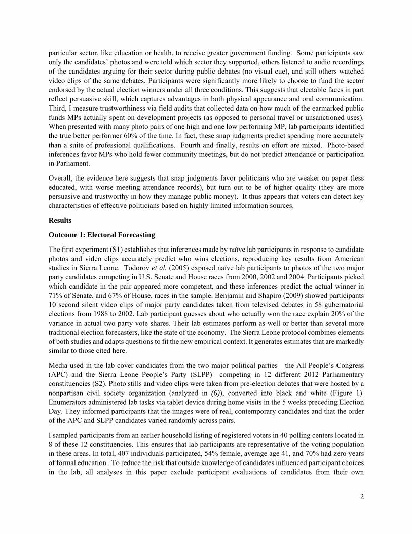
Media used in the lab cover candidates from the two major political parties—the All People’s Congress (APC) and the Sierra Leone People’s Party (SLPP)—competing in 12 different 2012 Parliamentary constituencies (S2). Photo stills and video clips were taken from pre-election debates that were hosted by a nonpartisan civil society organization (analyzed in (6)), converted into black and white (Figure 1). Enumerators administered lab tasks via tablet device during home visits in the 5 weeks preceding Election Day. They informed participants that the images were of real, contemporary candidates and that the order of the APC and SLPP candidates varied randomly across pairs.

I sampled participants from an earlier household listing of registered voters in 40 polling centers located in 8 of these 12 constituencies. This ensures that lab participants are representative of the voting population in these areas. In total, 407 individuals participated, 54% female, average age 41, and 70% had zero years of formal education. To reduce the risk that outside knowledge of candidates influenced participant choices in the lab, all analyses in this paper exclude participant evaluations of candidates from their own

 

3  

constituency and any others whom they recognized. While the number of observations is large (3,581), the number of races covered is small (12).

Lab participants first evaluated each candidate in a photo pair on leadership, corruption and attractiveness, and then guessed the candidate’s ethnic group. Participants were then shown the two photos together and asked “if you had to vote today, which candidate would you choose?” Similarly, for the video task participants watched 10 to 20 second video clips, with the sound on, of candidates speaking about which sector they would prioritize (if elected) for greater government funding. After each clip, participants rated the individual candidate on leadership, corruption, likeability and articulateness. Participants then compared the two and selected the one they would choose if they had to vote today. Finally, participants guessed which candidate in the pair belonged to the APC party. There was no specific time limit on these tasks.

Assessments of leadership, attractiveness, likeability and party identity closely follow the U.S. protocols. Evaluations of ethnicity, corruption and articulateness are tailored to the Sierra Leone context. Specifically, ethnicity strongly influences politics: there are two large ethnic groups—the Mendes in the South and the Temnes in the North—which each account for roughly one third of the national population and have strong historical ties to the SLPP and APC parties, respectively. If photos reveal candidate ethnicity, it is important to determine both the role of ethnicity in electoral forecasting, and whether it raises political economy concerns about printing photos on ballots. Corruption is also a salient issue and the prompt for this assessment focuses on the actual public funds that MPs control directly. It reads, “every year, Honorables receive 44 million Leones [roughly US$11,000] in the constituency facilitation fund (CFF). How much do you think this candidate would put in his own pocket and not use for development or for trips to his constituency?” The local phrase used for articulateness was “sabi tok,” which means “knows how to talk well” and also connotes persuasiveness.

Table 1 shows that “vote today” choices in the lab predict the subsequent election winners with probability greater than chance. At the individual-level, participants selected the eventual winner based on photos 55% of the time, which is greater than random guessing with a high degree of statistical significance (p-value < 0.000). Collapsed to the race-level, this yields a forecast that accurately predicts 75% of the 12 races studied and is significantly different from chance at 90% confidence. For videos, participants chose the eventual winner 55% of the time, which is significantly greater than random guessing (p<0.000). This yields a forecast accuracy of 67% at the race level, which is not statistically distinguishable from 50%.

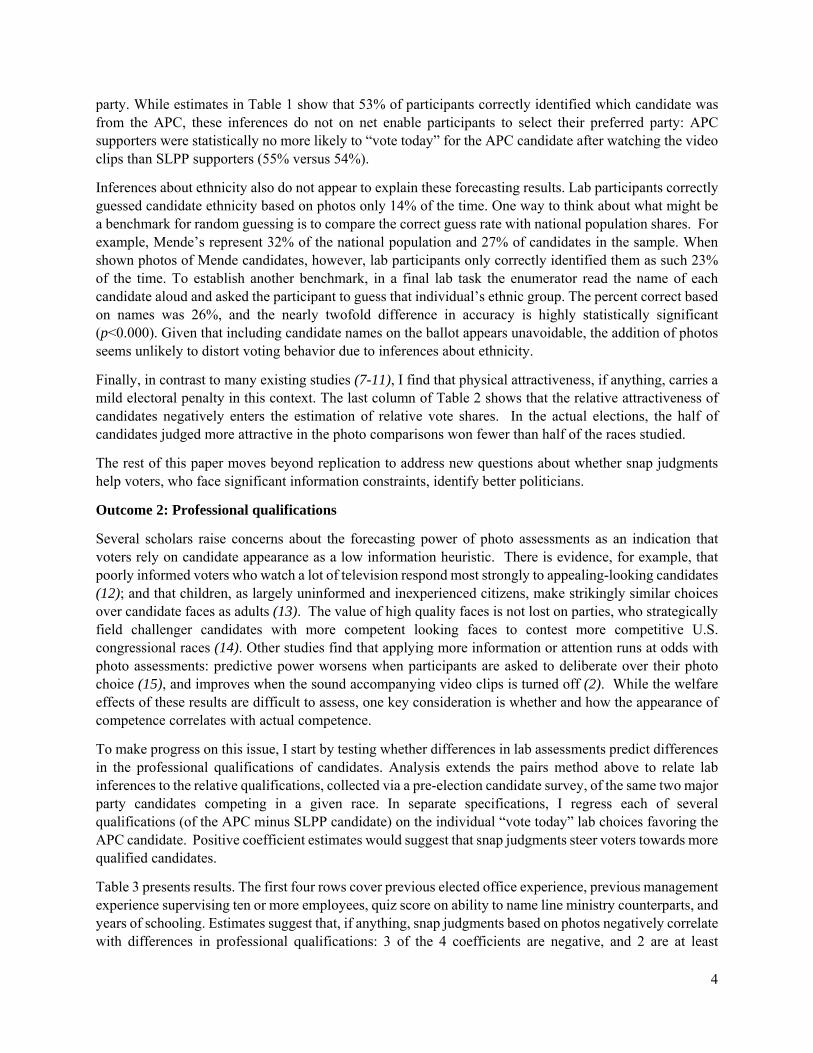
Figure 2 displays the forecasting power of participant assessments of leadership ability as opposed to “vote today” choices. It follows Todorov et al. noting one key divergence in protocol: I use the difference (APC minus SLPP) in individual leadership scores, while Todorov et al. use the choice variable “which candidate is more competent.” Each dot represents a race-level average. The upward sloping line shows that pre-election lab ratings of relative leadership ability positively correlate with subsequent differences in actual vote shares.

Table 2 presents regression counterparts. For photo “vote today” choices, regressing the actual APC party’s share of the two party vote on the share of lab participants who picked the APC candidate yields a positive coefficient of 1.02 (standard error 0.43), which is significant at 95% confidence. Estimates for the video condition are qualitatively similar but not statistically distinguishable from zero. The R2 indicates that lab assessments based on photos (videos) alone explain one third (one fifth) of the total variation in vote shares, which is markedly similar to estimates from the U.S. labs. The coefficient on leadership in column 3 estimates the slope of the line in Figure 2, which is positive and significant at 90% confidence.

Regarding mechanisms, I find little evidence that forecast accuracy is driven by inferences about ideology. Note that 75% of lab participants say they “will definitely” vote for the MP candidate from their preferred

 

4  

party. While estimates in Table 1 show that 53% of participants correctly identified which candidate was from the APC, these inferences do not on net enable participants to select their preferred party: APC supporters were statistically no more likely to “vote today” for the APC candidate after watching the video clips than SLPP supporters (55% versus 54%).

Inferences about ethnicity also do not appear to explain these forecasting results. Lab participants correctly guessed candidate ethnicity based on photos only 14% of the time. One way to think about what might be a benchmark for random guessing is to compare the correct guess rate with national population shares. For example, Mende’s represent 32% of the national population and 27% of candidates in the sample. When shown photos of Mende candidates, however, lab participants only correctly identified them as such 23% of the time. To establish another benchmark, in a final lab task the enumerator read the name of each candidate aloud and asked the participant to guess that individual’s ethnic group. The percent correct based on names was 26%, and the nearly twofold difference in accuracy is highly statistically significant (p<0.000). Given that including candidate names on the ballot appears unavoidable, the addition of photos seems unlikely to distort voting behavior due to inferences about ethnicity.

Finally, in contrast to many existing studies (7-11), I find that physical attractiveness, if anything, carries a mild electoral penalty in this context. The last column of Table 2 shows that the relative attractiveness of candidates negatively enters the estimation of relative vote shares. In the actual elections, the half of candidates judged more attractive in the photo comparisons won fewer than half of the races studied.

The rest of this paper moves beyond replication to address new questions about whether snap judgments help voters, who face significant information constraints, identify better politicians.

Outcome 2: Professional qualifications

Several scholars raise concerns about the forecasting power of photo assessments as an indication that voters rely on candidate appearance as a low information heuristic. There is evidence, for example, that poorly informed voters who watch a lot of television respond most strongly to appealing-looking candidates (12); and that children, as largely uninformed and inexperienced citizens, make strikingly similar choices over candidate faces as adults (13). The value of high quality faces is not lost on parties, who strategically field challenger candidates with more competent looking faces to contest more competitive U.S. congressional races (14). Other studies find that applying more information or attention runs at odds with photo assessments: predictive power worsens when participants are asked to deliberate over their photo choice (15), and improves when the sound accompanying video clips is turned off (2). While the welfare effects of these results are difficult to assess, one key consideration is whether and how the appearance of competence correlates with actual competence.

To make progress on this issue, I start by testing whether differences in lab assessments predict differences in the professional qualifications of candidates. Analysis extends the pairs method above to relate lab inferences to the relative qualifications, collected via a pre-election candidate survey, of the same two major party candidates competing in a given race. In separate specifications, I regress each of several qualifications (of the APC minus SLPP candidate) on the individual “vote today” lab choices favoring the APC candidate. Positive coefficient estimates would suggest that snap judgments steer voters towards more qualified candidates.

Table 3 presents results. The first four rows cover previous elected office experience, previous management experience supervising ten or more employees, quiz score on ability to name line ministry counterparts, and years of schooling. Estimates suggest that, if anything, snap judgments based on photos negatively correlate with differences in professional qualifications: 3 of the 4 coefficients are negative, and 2 are at least

 

5  

marginally significant. Similar results obtain for video inferences, with higher precision (S3). The negative estimate for education specifically is a potential cause for concern given that it is, by far, the most frequently cited quality of what participants think makes a good MP.

The next rows reveal no robust relationship between snap judgments and other political characteristics. It shows null results for incumbency status; internal party competition, as measured by the number of candidates who competed for the party symbol during the primary stage; membership in a ruling house, or family that is eligible to run for paramount chief in the traditional governance system; and expert assessments of candidate performance during the debate that the video clips were drawn from (S2).

Regarding demographics, there is no evidence that photos disadvantage women or young men, which is important given the historical marginalization of both groups in politics. The positive and marginally significant coefficient on gender implies that participants were more likely to “vote today” for female candidates. While one might interpret this as evidence for social desirability bias, note that all three of the female candidates in the sample won their seat. Scholars point to the disenfranchisement of young men as a driver of the civil war (1991 to 2002) (16). “Vote today” shares negatively (but not significantly) correlate with actual candidate age, providing no evidence for preferences favoring elder candidates. The age profile of sampled candidates was also not heavily skewed towards elders: mean of 47 years and range 33 to 67.

Outcome 3: Persuasion skills

The second candidate quality test evaluates whether the observed returns to electable faces capture intangible persuasive ability. This was implemented during a second lab experiment, which used the same pre-election media on candidates, but was fielded after the election (in January 2016).

I model this experiment loosely after Mobius and Rosenblatt (2006), who decompose the beauty wage premium of Hamermesh and Biddle (1994) into direct taste-based discrimination by employers and an indirect worker confidence channel (17, 18). Their indirect channel shows how physical attractiveness lends confidence to workers, a trait they convey even through non-visual oral communication, and enables them to negotiate higher wages. The persuasion lab similarly aims to evaluate both a physical appearance channel, where the “looks of a leader” add legitimacy to one’s policy proposal in the eyes of others, and an indirect channel, where looking like a leader creates opportunities to build communication skills.

The Sierra Leone lab covered 72 pairs of winning and losing candidates, each of whom argued for a specific sector to receive greater government funding during the pre-election debates. Some pairs are the actual two candidates in a given race, others are pairings across races (some within and others across parties). The modal sector advocated by candidates was education, followed by health, roads and agriculture. Lab protocols ask voters which of the sectors backed by the two candidates in the pair they would fund, under three conditions: priority sectors accompanied by candidate photos; oral recordings of the candidates’ arguments promoting the sector, with no visual cue; and audiovisual clips of the same arguments. The audio and video used here cover the candidate’s entire pitch made during the debate, so are longer and more coherent than the video snippets used earlier for electoral forecasting.

Enumerators introduced the task with the following script: “Each year, Parliament is responsible for approving the budget for the Government of Sierra Leone. Members of Parliament have the opportunity to influence what kinds of projects are prioritized in the country. There is a limited amount of funds, so some problems must receive more attention than others. I am going to show you photos [audio/video] of real Honorables (MPs) candidates and tell you what issue they think the government should spend more money on. These MPs are not from your constituency, but are from other parts of Sierra Leone.”

 

6  

This post-election lab allocated many distinct tasks across a new participant pool. I sampled 399 participants from a household listing of registered voters conducted one month prior to the lab: 51% were female, average age 38, and 53% had no formal schooling. To protect against participant inferences reflecting knowledge of MP performance, this lab was conducted in rural areas of 4 constituencies not represented by any MP in the sample. Recognition rates were below 1%.

Estimates in Table 4 suggest that candidates who subsequently won a seat are more persuasive than those who lost, under all three conditions. Specifically, 60.5% of lab participants selected the sector backed by the election winner’s photograph, which suggests that election winners have an advantage in the direct physical appearance channel of persuasion. Without any visual cue, 57.8% of (other) lab participants selected the winner’s sector based on audio arguments. This substantiates the idea that election winners have better oral communication skills. Both results are significantly greater than chance guessing at 99% confidence. The estimate for the video condition, which combines the visual and oral cues, is slightly larger than both of these (61.0%), but only statistically distinguishable when compared to the audio only condition (by 3.2 percentage points, p-value = 0.065). Results are robust to controlling for participants’ own sectoral preferences and partisanship (S4).

Together these findings provide one productivity-enhancing rationale for why facial features might enter the voter’s forecasting model: candidates with more electable faces tend to be more persuasive.

Outcome 4: Trustworthiness

I now turn to concrete measures of politician performance on the job. While these are the outcomes of ultimate interest, they are by nature only realized for election winners, so lab protocols here elicit relative evaluations among currently serving MPs. Analysis leverages rich data on the activities of 28 elected MPs over their first year and a half in office. I begin with inferences about trust and measures of public spending.

Results from a variety of disciplines provide some basis for the idea that trustworthiness might be observable in photos. One study finds evidence for a genetic component of trust by studying the behavior of twins in the classic trust game (19). Others find evidence for biological bases for trust via links to the neuropeptide oxytocin (20) and stress hormone cortisol (21). Another argues that the amygdala part of the brain automatically interprets certain facial features as untrustworthy in a way that is common across individuals (22). And, most directly related to the work here, Duarte, Siegel and Young (2012) show that potential borrowers on an online lending platform who appear more trustworthy in photos do, in fact, have higher credit scores and lower default rates (23).

Widespread concern about corruption in politics, paired with weak institutional checks on elected officials, makes trustworthiness particularly important in new democracies like Sierra Leone. For the public money analyzed here, the constituency facilitation fund (CFF), the Ministry of Finance records only whether the MP signed for these funds into his or her own personal bank account and requires no further reporting or monitoring. The trustworthiness of individual politicians is thus a key determinant of whether this money is put to public or private use.

We measured how the CFF was spent in practice via extensive field audits that tracked each expenditure line item that an MP claimed (in a 2014 survey) to have used for development to its source in the MP’s home constituency. Any remaining unverified funds were either spent on legitimate personal transport costs for MP travel to and from his or her constituency, or diverted to other unsanctioned uses. Voters strongly prefer the CFF to be spent on development: 100% of lab participants said “most” or “all” of the CFF should go to development and not to travel expenses; and demonstrate some tolerance for diversion: 32% thought it was okay for MPs to “chop” a “little” bit of the money for themselves. In practice, diversion of the CFF

 

7  

is substantial—e.g., the audits verified zero development expenditures for 6 of the sampled MPs—and exceeds what would constitute an acceptably small amount.

The trust experiment was implemented in the same post-election lab described above for persuasion. It used the official MP headshots posted on the website of Parliament, converted into black and white and rescaled for comparability. I formed pairs of photos by first ordering the 27 MPs by their actual performance on the CFF spending metric. I then made 55 different pairings between those in the top and bottom half of the distribution, enforcing a minimum number of ordinal performance ranks between each member of a pair. Enumerators introduced the task by explaining what the CFF is, what its intended uses are, and that we had checked how much of this money the MPs actually spent on development. They told participants that one MP in every pair spent more than the other, that the order would be mixed, and asked them to “Do your best to guess which MP spent more of the CFF on development and put less in his own pocket.”

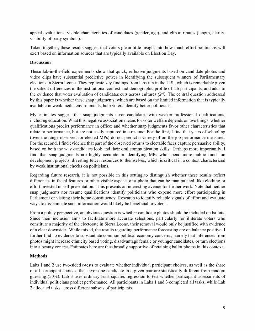
Across 55 photo pairs, lab participants chose the MP who in fact performed better 54.2% of the time, which is significantly better than random guessing at 99% confidence. Figure 3 plots the distribution of correct guesses across the photo pairings. The vertical line shows that for only 33% of the photo pairs was the proportion of correct lab selections below 0.50.

Table 5 compares the predictive power of these photo inferences to a range of candidate qualifications. I leverage the fact that the same MP was compared to several different peers (4 on average) in the lab photo pairings. Collapsing and reformatting the data generates 110 observations of MP trustworthiness vote shares by pair, which I regress on fixed effects for the 27 MPs in the sample. The estimated coefficients capture the intangible features that make a particular MP appear relatively more or less trustworthy than his peers in official headshot photos. I then evaluate the forecast accuracy of this measure relative to the observable characteristics used in Table 3.

Estimates suggest that these MP-specific fixed effects strongly outperform the suite of observable characteristics in predicting who actually spent the CFF on development. The coefficient on inferred trustworthiness is large, positive and highly statistically significant. To provide a sense of magnitude, moving from the 25th to 75th percentile of the inferred trust distribution corresponds to spending nearly $7,000 more on development projects, or 62% of the annual allotment. By contrast, only one coefficient on the observable characteristics is significant on its own. Notably, this is years of schooling, which negatively predicts development spending. An F-test cannot reject that all coefficients for observable qualifications are jointly equal to zero, while the test for inferred trustworthiness is highly significant. Note that the R2 falls by nearly half when the inferred trust measure is excluded from the specification (from 0.54 to 0.28).

Given the small number of observations compared to explanatory variables, I also ran two way “horse races” between the inferred trustworthiness measure and each of the nine observable characteristics separately. The difference in coefficients on the intangible versus observable measure is positive and significant at 90% (95%) confidence for all 9 (7) of these tests (not shown).

These results suggest that voter inferences based on politician appearance are more accurate predictors of spending performance than their professional qualifications. Additional analyses show that the predictive power of trust inferences is robust to controlling for participant assessments of how wealthy candidates look (S5); and outperforms inferences based on audio recordings of what candidates say they will do with the money (S6).

Outcome 5: Effort

The final experiments concern politician effort, which I measure and test in two ways.

 

8  

The first applies the trustworthiness protocol above to effort exerted in holding public meetings. I order 28 sitting MPs according to the observed number of meetings they held, and then form 56 headshot photo pairs between high and low performers. Data on meetings was collected during the CFF field audits, and analysis uses the average number of meetings reported among many community surveys fielded in the MP’s home constituency. Enumerators introduced the lab task with the following prompt: “It is the Honorable’s job to represent the people from their constituency, and they can make sure they are doing a good job by visiting their constituency regularly. I am now going to show photos of real Honorables who are not from your constituency, but are from other parts of Sierra Leone. We checked how often they visited their own constituencies. In each pair, one MP visited his constituency more than the other, and the order is mixed up. Do your best to guess which MP works harder by visiting his constituency more often.”

In contrast to the results for trust, participant inferences systematically favor weaker performers for effort: they selected the MP who actually held more meetings 46% of the time, which is significantly worse than random guessing at 99% confidence. Alternative forecasters, however, appear equally ineffective. I ran a similar series of comparisons between inferred effort and observable predictors as completed for trustworthiness (S7). None of the estimated coefficients on the intangible or observable characteristics individually predicts effort in organizing public meetings. As a group, the observables have greater explanatory power: the F-test rejects the null that all nine coefficients are jointly equal to zero at 90% confidence; and adding the inferred effort measure explains no additional variance.

The second effort test was implemented in a third lab-in-the-field experiment, which was conducted in 2013, shortly after the election (S8). It exposed participants to 20 second video clips, with sound, of the previous cohort of incumbent MPs making public comments in the well of Parliament during their tenure in office (2007-2012). Footage comes from the Sierra Leone Broadcasting Corporation (akin to C-SPAN). Clips were available for 45 of the 112 incumbent MPs. Enumerators explained that participants would watch a series of video clips of MPs from the previous Parliament. After each video, participants rated the speaker on measures of appeal (leadership, lack of corruption, articulateness, likeability, similarity of priorities, and hard work) and then indicated whether they would vote today for the MP. Unlike all labs above, this lab elicits inferences about individuals and not comparisons within pairs.

Lab participants were sampled in two ways: i) rural participants were sampled from an earlier listing exercise covering thirty households in each of 16 polling centers; and ii) enumerators selected urban participants from crowds waiting at public transport hubs and shop owners in three major towns. There were 965 participants in total, in six constituencies, 49% female, average age 38, and 54% (24%) of rural (urban) participants had zero years of schooling.

Outcome data for attendance and participation was compiled from Parliamentary administrative records and covers all sittings from 2009 to 2012, approximately 150 in total. Analysis uses the percent of sittings for which the MP was present or made any public comments, respectively. Measures of popularity and visits were compiled from a national opinion poll conducted by telephone in early 2012, several months before the election. Phone numbers were sampled from call logs of a major mobile telecommunications provider and assigned to constituencies based on tower locations. Popularity refers to the percent of poll respondents who said they wanted their incumbent MP to be re-elected, and visits refers to the percent who said their incumbent MP had visited their constituency at least once during the past year.

Table 6 presents results from separate specifications that regress each of the four outcome measures on the share of lab participants who said they would “vote today” for that incumbent MP. The coefficient for popularity is positive and significant at 95% confidence. There is no statistically significant relationship between lab choices and any of the three effort measures. Results (not shown) are robust to including the

 

9  

appeal evaluations, visible characteristics of candidates (gender, age), and clip attributes (length, clarity, visibility of party symbols).

Taken together, these results suggest that voters glean little insight into how much effort politicians will exert based on information sources that are typically available on Election Day.

Discussion

These lab-in-the-field experiments show that quick, reflexive judgments based on candidate photos and video clips have substantial predictive power in identifying the subsequent winners of Parliamentary elections in Sierra Leone. They replicate key findings from labs run in the U.S., which is remarkable given the salient differences in the institutional context and demographic profile of lab participants, and adds to the evidence that voter evaluation of candidates cuts across cultures (24). The central question addressed by this paper is whether these snap judgments, which are based on the limited information that is typically available in weak media environments, help voters identify better politicians.

My estimates suggest that snap judgments favor candidates with weaker professional qualifications, including education. What this negative association means for voter welfare depends on two things: whether qualifications predict performance in office; and whether snap judgments favor other characteristics that relate to performance, but are not easily captured in a resume. For the first, I find that years of schooling (over the range observed for elected MPs) do not predict a variety of on-the-job performance measures. For the second, I find evidence that part of the observed returns to electable faces capture persuasive ability, based on both the way candidates look and their oral communication skills. Perhaps more importantly, I find that snap judgments are highly accurate in identifying MPs who spend more public funds on development projects, diverting fewer resources to themselves, which is critical in a context characterized by weak institutional checks on politicians.

Regarding future research, it is not possible in this setting to distinguish whether these results reflect differences in facial features or other visible aspects of a photo that can be manipulated, like clothing or effort invested in self-presentation. This presents an interesting avenue for further work. Note that neither snap judgments nor resume qualifications identify politicians who expend more effort participating in Parliament or visiting their home constituency. Research to identify reliable signals of effort and evaluate ways to disseminate such information would likely be beneficial to voters.

From a policy perspective, an obvious question is whether candidate photos should be included on ballots. Since their inclusion aims to facilitate more accurate selections, particularly for illiterate voters who constitute a majority of the electorate in Sierra Leone, their removal would only be justified with evidence of a clear downside. While mixed, the results regarding performance forecasting are on balance positive. I further find no evidence to substantiate common political economy concerns, namely that inferences from photos might increase ethnicity based voting, disadvantage female or younger candidates, or turn elections into a beauty contest. Estimates here are thus broadly supportive of retaining ballot photos in this context.

Methods

Labs 1 and 2 use two-sided t-tests to evaluate whether individual participant choices, as well as the share of all participant choices, that favor one candidate in a given pair are statistically different from random guessing (50%). Lab 3 uses ordinary least squares regression to test whether participant assessments of individual politicians predict performance. All participants in Labs 1 and 3 completed all tasks, while Lab 2 allocated tasks across different subsets of participants.

 

10  

References

(1) Todorov A, Mandisodza A, Goren A, Hall C (2005) Inferences of Competence from Faces Predict Election Outcomes, Science 308:1623-1626.

(2) Benjamin D, Shapiro J (2009) Thin-slice Forecasts of Gubernatorial Elections, Review of Economics and Statistics 91:523-536.

(3) Ambady N, Rosenthal R (1992) Thin Slices of Expressive Behavior as Predictors of Interpersonal Consequences: A Meta-Analysis, Psychological Bulletin 11:256-274.

(4) Henrich J, Heine S, Norenzayan A (2010) The weirdest people in the world? Behavioral and Brain Sciences 33:61-135.

(5) Open Science Collaboration (2015) Estimating the reproducibility of psychological science, Science 349: aac4716.

(6) Bidwell K, Casey K, Glennerster R (2016) Debates: Voting and Expenditure Responses to Political Communication, Stanford GSB working paper 3066.

(7) Banducci S, Karp J, Thrasher M, Rallings C (2008) Ballot Photographs as Cues in Low Information Elections, Political Psychology 29:903-917.

(8) Berggren N, Jordahl H, Poutvaara P (2010) The Looks of a Winner: Beauty and Electoral Success, Journal of Public Economics 94:8-15.

(9) Lutz G (2010), The Electoral Success of Beauties and Beasts, Swiss Political Science Review 16:457-480.

(10) Rosar U, Klein M, Beckers T (2008) The Frog Pond Beauty Contest: Physical Attractiveness and Electoral Success of the Constituency Candidates in the North Rhine Westphalia State Election of 2005, European Journal of Political Research 47:64-79.

(11) Ahler D, J Citrin, M Dougal, G Lenz (forthcoming) Can Your Face Win You Votes? Experimental Tests of Canddiate Appearance’s Influence on Electoral Choice, Political Behavior.

(12) Lenz G, Lawson C (2011) Looking the Part: Television Leads Less Informed Citizens to Vote Based on Candidates’ Appearance, American Journal of Political Science 55:574-589.

(13) Antonakis J, Dalgas O (2009) Predicting Elections: Child's Play! Science 323:1183. (14) Atkinson M, Enos R, Hill S (2009) Candidate Faces and Election Outcomes: Is the Face-Vote

Correlation Caused by Candidate Selection, Quarterly Journal of Political Science 4:229-249. (15) Ballew II C, Todorov A (2007) Predicting political elections from rapid and unreflective face

judgments, Proceedings of the National Academy of Sciences 104:17948-17953. (16) Richards P (1996) Fighting for the Rainforest: War, Youth and Resources in Sierra Leone.

London: James Currey. (17) Mobius M, Rosenblatt T (2006) Why Beauty Matters, American Economic Review 96:222-235. (18) Hamermesh D, Biddle J (1994) Beauty and the Labor Market, American Economic Review

84:1174-1194. (19) Cesarini D, Dawes C, Fowler J, Johannesson M, Lichtenstein P, Wallace B (2008) Heritability of

cooperative behavior in the trust game, Proceedings of the National Academy of Sciences 105:3721-3726.

(20) Kosfeld M, Heinrichs M, Zak P, Fischbacher U, Fehr E (2005) Oxytocin increases trust in humans, Nature 435:673-676.

(21) Takahashi T, Ikeda K, Ishikawa M, Kitamura N, Tsukasaki T, Nakama D, Kameda T (2005) Interpersonal trust and social stress-induced cortisol elevation, NeuroReport 16:197-199.

(22) Engell A, Haxby J, Todorov A (2007) Implicit Trustworthiness Decisions: Automatic Coding of Face Properties in the Human Amygdala, Journal of Cognitive Neuroscience 19:1508-1519.

(23) Duarte J, Siegel S, Young L (2012) Trust and Credit: The Role of Appearance in Peer-to-peer Lending, Review of Financial Studies 25: 2455-2483.

 

11  

(24) Lawson C, Lenz G, Baker A, Myers M (2010) Looking Like A Winner: Candidate Appearance and Electoral Success in New Democracies, World Politics 62:561-93.

(25) Angrist J, Pischke J (2009) Mostly Harmless Econometrics, Princeton: Princeton University Press.

(26) Cameron A, Gelbach J, Miller D (2008) Bootstrap-based Improvements for Inference with Clustered Errors,” Review of Economics and Statistics 90:414-42.

 

12  

Figure 1: Example of candidate photo pair

If you had to vote today, which candidate would you choose?

Figure 2: Differences in actual vote shares are increasing in inferred leadership

The horizontal axis measures the mean difference in participant leadership assessments of the APC minus the SLPP candidate photos. The vertical axis measured the actual difference in the APC minus the SLPP candidate’s subsequent vote share in the 2012 Parliamentary election.

-.50

.51

Diff

eren

ce in

act

ual A

PC

- S

LPP

vot

e sh

ares

-.5 0 .5Mean difference APC - SLPP inferred leadership - photos

 

13  

Figure 3: Inferred trustworthiness of elected MPs predicts public spending

This graph plots the cumulative distribution function (CDF) of the share of correct lab participant guesses about which MP in a photo pair actually spent more of their discretionary public funds on development projects (N = 55 pairs).

Table 1: Snap judgments accurately predict electoral outcomes

Assessment Percent p-value (≠ 50%)

Observations

Photo condition Participant would vote today for actual winner 55.1*** 0.000 3,581 evaluations of candidates Share of participants would vote today for actual winner 75.0* 0.082 12 Parliamentary races Participant gave actual winner higher leadership score 59.7*** 0.000 976 evaluations of candidates Share of participants who gave actual winner higher leadership score

58.3 0.586 12 Parliamentary races

Video condition Participant would vote today for actual winner 54.9*** 0.000 3,581 evaluations of candidates Share of participants would vote today for actual winner 66.7 0.266 12 Parliamentary races Participant identified the actual APC party candidate 52.7*** 0.001 3,581 evaluations of candidates Share of participants who identified actual APC party candidate

58.3 0.586 12 Parliamentary races

Reported p-values are based on two-sided t-tests that the estimated percent correct does not equal 50%. Significance levels indicated by * p < 0.10, ** p < 0.05 and *** p < 0.001. Rows 3 and 4 limit the sample to participants who gave different leadership scores to candidates in a given photo pair.

0.2

.4.6

.81

Cum

ulat

ive

dens

ity o

f MP

pho

to p

airs

.4 .5 .6 .7 .8Share of participants who correctly identify more trustworthy MP

 

14  

Table 2: Regression estimates of snap judgment forecast accuracy

Dependent variable: APC share of the two party vote

Difference APC-SLPP vote shares

Share who would vote today for APC (photos) 1.021** (0.427)

Share who would vote today for APC (videos) 0.727 (0.460) Difference APC-SLPP leadership evaluation (photos) 1.135*

(0.618) -1.569 (2.660)

Difference APC-SLPP (not) corrupt evaluation (photos) 5.222* (2.547)

Difference APC-SLPP attractiveness evaluation (photos) -1.609* (0.707)

R2 0.36 0.20 0.25 0.63 Observations 12 12 12 12

Ordinary least squares coefficient estimates with standard errors that are the maximum of (unadjusted OLS, HC2 corrected) to accommodate the small number of races, following (25). Significance levels indicated by * p < 0.10, ** p < 0.05 and *** p < 0.001.

Table 3: Snap judgments negatively correlate with candidate resume qualifications

“Vote today” for the APC candidate in the photo pair Difference in characteristics (Candidate APC – SLPP): Coefficient Standard error Bootstrap t Previous elected office experience 0.022 (0.090) 0.792 Previous management experience with 10+ employees -1.222* (0.082) 0.064 Quiz score for naming line ministry counterparts -0.003 (0.262) 1.000 Years of schooling -0.373** (0.317) 0.032 Incumbency status 0.041 (0.045) 0.324 Competition for own party symbol 0.176 (0.272) 0.404 Membership in a ruling house -0.006 (0.140) 0.936 Expert panel assessment of debate performance 4.956 (5.473) 0.220 Age -1.013 (2.324) 0.620 Female candidate 0.123* (0.078) 0.010 Observations (evaluations of candidate pairs) 3,581 Clusters (races) 12

Each row reports coefficient and standard error from a separate ordinary least squares regression of the relative (APC minus SLPP) candidate characteristic listed on whether lab participants selected the APC as their “vote today” choice in the lab photo task. Significance levels indicated by * p <0.10, ** p <0.05, *** p <0.01 based on the pairs cluster bootstrap t with 500 replications (26). Specifications include household stratification bins used in a related experiment (6).

Table 4: Snap judgments and persuasion skills

Pick winner’s project Percent p-value (≠ 50%) Percent who selected winner’s project in pairs of photos 60.5*** 0.001 Percent who selected winner’s project in pairs of oral arguments 57.8*** 0.001 Percent who selected winner’s project in pairs of video arguments 61.0*** 0.000 Observations 72 candidate pairs

Significance levels indicated by * p <0.10, ** p <0.05, *** p <0.01.

 

15  

Table 5: Snap judgments predict public spending more accurately than resume characteristics

Dependent variable: Actual CFF spending on development projects Coefficient Std. error Coefficient Std. error Trustworthiness inferred from photo snap judgments 569.66** (196.31) Previous elected office experience -13.05 (50.45) 34.47 (57.73) Previous management experience with 10+ employees -3.28 (34.15) 13.08 (40.75)Quiz score for naming line ministry counterparts -9.48 (17.76) -9.14 (21.49)Years of education -21.10* (10.73) -12.93 (12.53)Incumbency status -21.83 (58.66) -62.56 (68.90)Competition for own party symbol -9.97 (6.62) -10.62 (8.00)Membership in a ruling house -33.80 (36.28) -15.44 (43.22)Age 1.57 (1.72) 1.29 (2.08)Female candidate -39.17 (59.81) 4.54 (70.04) Prob > F on intangible 0.011 Prob > F on observables 0.462 0.891 R2 0.542 0.284 Observations 27 MP photo pairs

Ordinary least squares regression. Significance levels indicated by * p <0.10, ** p <0.05, *** p <0.01. Standard errors are the maximum of (unadjusted OLS, HC2 corrected). These 28 MPs participated in a randomized experiment as part of a related research project (6), so all photo pairings are formed within that project’s treatment group assignment and regressions include an assignment indicator. CFF spending is not observed for one of the 28 MPs whose election was contested so did not take office until a year later and did not receive the first annual CFF. Missing survey responses regarding observable characteristics of two MPs are replaced based on their photo, electoral records and imputation at the sample mean. One characteristic from Table 3, expert assessment of debate performance, is omitted here as it is available for only half the sample. The dependent variable is total funds verified as spent on development divided by the annual CFF allotment.

Table 6: Snap judgments do not predict MP effort in office

Relationship to “vote today” choices in the lab Dependent variable Coefficient Standard error p-value Observations Popularity 0.882** (0.394) 0.025 44 Attendance in Parliamentary sittings -0.042 (0.180) 0.815 45 Participation in Parliamentary sittings -0.328 (0.367) 0.372 45 Visits to home constituency 0.347 (0.213) 0.213 44

Ordinary Least Squares regressions with robust standard errors. Significance levels indicated by * p <0.10, ** p <0.05, *** p <0.01.

 

S1  

Supplementary Information for “Snap judgments: Voter inferences based on candidate photos predict electoral success and politician quality” by K. Casey

S1: Overview of the lab-in-the-field experiments

Lab Field date Politicians covered Main tasks completed by lab participants 1 October 2012 MP candidates competing in

the November 2012 Election Evaluation of candidate photo pairs

Evaluation of candidate video pairs

Inferences about ethnicity based on names

2 January 2016 MP candidates competing in the November 2012 Election

Winning MPs serving in Parliament 2012 - present

Evaluation of winning/losing candidate pairs filmed in 2012 pre-election debates

Inferences about elected MP trustworthiness and effort in office

3 February 2013 Incumbent MPs who served in Parliament 2007 - 2012

Evaluation of individual MPs in video footage of Parliamentary sittings

S2: Additional information on Lab 1

Race sample These 12 races were selected from the population of 112 based on pre-election estimates that they would be relatively competitive. Vote share data comes from the National Electoral Commission (NEC) official returns for 11 of the 12 races. I calculate vote shares for the one remaining race based on exit poll data, as this race was contested in the courts and NEC did not release voting returns. All results in Table 1 are robust to excluding this race, save the estimate in Row 2 falls below the 90% confidence level.

Recognition rates

Recognition rates for candidates outside lab participants’ home constituency were low, at 2.2%. Evaluations of candidates from lab participants’ home constituency are excluded.

Table 1 robustness check

All estimates in Table 1 hold when the sample is limited to the 9 races where both candidates were male, save the estimate in Row 2 falls below the 90% confidence level and the estimate in Row 8 becomes statistically significant at 90% confidence.

Figure 2 alternative specification

There is an even tighter relationship between leadership inferences and the “vote today” choices made by other lab participants, as compared to realized election outcomes. Since all participants completed the rankings and “vote today” selections, I randomly split the sample and correlate the leadership inferences from one half with the “vote today” choices of the other half. As in Todorov et al., the Spearmen correlation for simulated votes is markedly larger (0.90, p<0.001, N=12 races) than that for actual vote shares (0.52, p<0.080). Their interpretation, which also seems reasonable in this context, is that actual vote choices reflect additional pieces of information beyond first impressions, diluting the relationship between the snap judgment of photos and the eventual choice in the polling booth.

Ethnicity from photos

Participants were four times more likely to correctly identify the ethnicity of a candidate from their own group, compared to those from other groups (42 versus 11%). And yet, because candidates and lab participants come from many different ethnic groups, participants evaluated co-ethnics in only 10% of photo pairs, and were thus overall no more likely to “vote today” for co-ethnic candidates. Conditional on

 

S2  

correctly guessing a given candidate’s ethnicity, participants were only marginally more likely to vote for co-ethnics than not (by 5 percentage points).

Ethnicity from names

There are four small ethnic groups for which the rate of correct guessing was higher than their population share, however the highest correct rate was 12%.

Attractiveness penalty

Since assessments of leadership, corruption and attractiveness in Table 2 column 4 are all closely correlated with each other, I also ran a regression of differences in vote shares on the relative attractiveness rating alone. The estimated coefficient is positive in sign but not statistically distinguishable from zero.

Expert panel We convened a panel of 25 government and civil society experts to score candidates' performance in the debates as part of a related research project (6). Experts scored each candidate's response on a 10 point scale to each of several policy questions. Analysis uses the total score averaged across multiple experts.

S3: Video condition snap judgments negatively correlate with candidate resume qualifications

“Vote today” for the APC candidate in the video pair Difference in characteristics (Candidate APC – SLPP): Coefficient Standard error Bootstrap t Previous elected office experience 0.056 (0.087) 0.416 Previous management experience with 10+ employees -0.175* (0.116)  0.060 Quiz score for naming line ministry counterparts -0.163 (0.306)  0.460 Years of schooling -0.577*** (0.353)  0.004   Incumbency status 0.085 (0.059)  0.280 Competition for own party symbol 0.327 (0.305)  0.152 Membership in a ruling house -0.023 (0.157)  0.804 Expert panel assessment of debate performance 3.315 (5.724)  0.492   Age -0.684 (2.359)  0.724 Female candidate 0.114* (0.075)  0.010   Observations (evaluations of candidate pairs) 3,581 Clusters (races) 12

Each row reports coefficient and standard error from a separate ordinary least squares regression of the relative (APC minus SLPP) candidate characteristic listed on whether lab participants selected the APC as their “vote today” choice in the lab video task. Significance levels indicated by * p <0.10, ** p <0.05, *** p <0.01 based on the pairs cluster bootstrap t with 500 replications (26). Specifications include household stratification bins used in a related experiment (6).

 

S3  

S4: Snap judgments and intangible persuasion skills

Pick first project in pair Coefficient standard error First project endorsed by winning candidate 0.661** (0.194) First project aligns with participant’s own public goods preference 1.760** (0.129) First project endorsed by candidate from participant’s own party 0.185 (0.141) Constant -1.404** (0.147) Prob> Chi2 0.000 Observations 1,422 evaluations of candidate pairs

This table explores two alternative mechanisms for the persuasion results in main text Table 4: sectoral alignment and partisanship. First, successful candidates might argue for sectors more in line with voter preferences. Indeed the project endorsed by the winning candidate in a pair ranked higher than the losers’ in lab participants’ own sectoral rankings 57% of the time. Second, while sector is generally party neutral, the ruling APC party oversaw a major healthcare reform, so advocating for health might reveal party identity. To test these channels, this table presents results from a logistic regression that predicts when a lab participant chose the first project among the two advocated in a given candidate pair. The positive and significant coefficients on the first project being endorsed by a winning candidate and the first project ranking higher in the participant’s own rankings suggest that both persuasiveness and sectoral preferences matter for deciding which project to fund. By contrast, the coefficient on the first project being endorsed by the candidate from the voter’s own party is small in magnitude and not statistically distinguishable from zero, providing little evidence for a partisanship channel. Significance levels indicated by * p <0.10, ** p <0.05, *** p <0.01. Coefficients are from a logistic regression with standard errors clustered by candidate pair. These estimates are based on the video condition, estimates for the photo and oral argument conditions are similar in magnitude and precision.

S5: Correlation between inferences about trustworthiness and wealth, and actual CFF spending

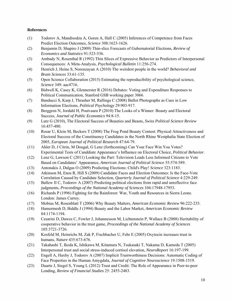
Theoretically the relationship between inferences about wealth and trustworthiness on the one hand, and actual MP spending on the other, could go either way: MPs who look poorer could be assumed to have a greater need to divert resources towards personal expenses (and do); or, those who look wealthier could be assumed to have enriched themselves previously (and continue to do so). To test this, a separate set of 40 lab participants viewed the same 55 photo pairs and picked which one in the pair “looks richer.” Figure S5 fits a nonparametric relationship between the proportion of lab participants who correctly identified the MP who spent more on development (labeled, “less corrupt”) and the proportion who thought that same MP looked like the wealthier one in the pair. The upward sloping line shows a strong positive correlation between the proportion of lab participants who correctly identified the less corrupt MP in the photo pairs and the proportion of (other) lab participants who thought that the less corrupt MP in the photo pair looked wealthier. This suggests that the rate of correct inference is highest where the less corrupt MP appeared wealthier. In fact, inferences in the bottom third of the relative wealth appearance pairs, where the less corrupt MP looked poorer, are significantly worse than random guessing (47.3% correct, p-value = 0.075, N=18 pairs); while those in the top third of the distribution, where the less corrupt MP looked wealthier, are substantially more accurate than random guessing (62.3% correct, p-value = 0.001, N=18 pairs). Inference accuracy in the middle third, where the two MPs appeared comparable in wealth terms, is greater than 50% but not significantly so (53.0%, p-value 0.163, N=19 pairs). In a two way “horse race,” participant inferences about which candidate will spend more on development outperform inferences about who is wealthier: the regression coefficient for trust is positive and significant (2.36, standard error 0.69), while that for wealth is negative and insignificant (-0.46, s.e. 0.49, N = 55 pairs).

.4.5

.6.7

.8P

ropo

rtion

cor

rect

ly id

entif

y le

ss c

orru

pt M

P

.2 .4 .6 .8Proportion think less corrupt MP looks wealthier

bandwidth = .8

Lowess smoother

 

S4  

S6: Snap judgments based on how politicians look versus what they say

Assessment Percent correct

p-value (≠50%)

Observations

Percent picks MP who spent more CFF on development - photo 52.6 0.139 27 MP pairs Participants pick MP who spent more CFF on development – photo 52.6* 0.096 1,052 lab evaluations Percent picks MP who spent more CFF on development - audio 46.8 0.447 27 MP pairs Participants pick MP who spent more CFF on development – audio 47.0* 0.054 1,032 lab evaluations Percent picks MP who spent more CFF on development - video 50.2 0.958 27 MP pairs Participants pick MP who spent more CFF on development - video 50.1 0.926 1,029 lab evaluations

Table S6 compares the discriminatory power of inferences based on photos to that of audio and video clips of MPs describing their plans for the CFF. The clips are drawn from the pre-election debates and cover the candidates’ complete answer to the question of how they would allocate these public funds if elected. This task follows the same protocol described for the photo condition under outcome 4, however as only half of the sampled MPs participated in the pre-election debates, the number of pairwise comparisons falls from 54 to 27 which limits statistical power. I compare the accuracy of correctly identifying the better performer across the photo, audio and video conditions for this subset of pairs. The conditions correspond to different lab tasks, which were completed by non-overlapping sets of participants. It appears that most of the forecast accuracy comes from physical impressions: the percent of correct guesses for the audio condition is 5.8 percentage points lower than for photos, which is sizeable yet not statistically significant in the pair-level estimates (p-value = 0.244). Accuracy in the video condition, which combines audio and visual cues, is statistically larger than audio only (p-value=0.099) and indistinguishable from the photo condition. These estimates suggest that voter assessments based on how politicians look more reliably predict spending performance than those based on what the candidates say. Reported p-values are based on two-sided t-tests. Significance levels indicated by * p < 0.10, ** p < 0.05 and *** p < 0.001.

S7: Neither snap judgments nor resume characteristics predict effort holding meetings

Dependent variable Actual number of meetings held with constituents Coefficient Std. error Coefficient Std. error Effort inferred from photo snap judgments -0.167 (5.763)  Previous elected office experience -0.823 (0.951) -0.832 (0.871)Previous management experience with 10+ employees -0.462 (0.709) -0.461 (0.688)Quiz score for naming line ministry counterparts 0.638 (0.383) 0.635* (0.351)Years of education 0.343 (0.270) 0.338 (0.211)Incumbency status 0.760 (1.075) 0.762 (1.041)Competition for own party symbol -0.031 (0.155) -0.033 (0.135)Membership in a ruling house 0.718 (0.841) 0.729 (0.727)Age -0.038 (0.033) -0.038 (0.032)Female candidate -1.156 (1.210) -1.161 (1.158)    Prob > F on intangible 0.977 Prob > F on observables 0.086 0.063 R2 0.594 0.594 Observations 28 MP photo pairs

Ordinary least squares regression. Significance levels indicated by * p <0.10, ** p <0.05, *** p <0.01. Standard errors are the maximum of (unadjusted OLS, HC2 corrected). These 28 MPs participated in a randomized experiment as part of a related research project (6), so all photo pairings are formed within that project’s treatment group assignment and regressions include an assignment indicator. Missing survey responses regarding observable characteristics of two MPs are replaced based on their photo, electoral records and imputation at the sample mean. One characteristic from Table 3, expert assessment of debate performance, is omitted here as it is available for only half the sample.

S8: Additional information for Lab 3

Clip sample Clips were available for 45 of 112 sitting MPs. Remaining MPs either never spoke publicly in Parliament or only spoke during sessions that were not recorded or were of poor film quality.

Recognition rates

Running the lab shortly after these MPs term in office completed carries the risk that respondents may have been familiar with the MPs’ performance. To mitigate this risk, I again drop participant evaluations that concern either the MP from their home

 

S5  

constituency or one that they recognize. Recognition rates were low: 3.3% for MPs from other constituencies and 5.7% for participant’s own MP.

Vote coding Unlike in the other labs, the response options for “would you vote today” included a “maybe” option. The outcome variable in Table 6 is coded to 1 if “yes,” 0.5 if “maybe,” and 0 if “no.”