Small Antennas for High Frequencies

Iulian Rosu, YO3DAC / VA3IUL, http://www.qsl.net/va3iul/

This is about Small Antenna types and their properties which can help choosing proper antenna for high-frequency wireless communications as: two-way radio, microwave short links, repeaters, radio beacons or wireless telemetry.

Basic Antenna Theory

Every structure carrying RF current generates an electromagnetic field and can radiate RF power to some extent.

A transmitting antenna transforms the Radio Frequency (RF) energy produced by a radio transmitter into an electromagnetic field that is radiated through space.

A receiving antenna it transforms the electromagnetic field into RF energy that is delivered to a radio receiver.

Most practical antennas are divided in two basic classifications: MARCONI Antennas (quarter-wave, which is the Monopole and derivates). HERTZ Antennas (half-wave, which is the Dipole and derivates).

Forming a radio wave

When an alternating electric current flows through a conductor (wire), Electric-E and Magnetic-H fields are created around the conductor.

If the length of the conductor is very short compared to a wavelength (<< λ/4), the electric and magnetic fields will decrease dramatically within a distance of one or two wavelengths.

However, as the conductor is lengthened, the intensity of the fields enlarges and part of the energy escapes into the space. When the length of the conductor approaches a quarter of a wavelength (λ/4) at the frequency of the applied alternating current, most of the energy will escape in the form of electromagnetic radiation.

Antenna Radiation

At a given frequency, there is impossible to make a small antenna to radiate like a big antenna.

A conductor once connected to a transmitter source, it begins to oscillate electrically, causing the wave to convert the transmitter power into an electromagnetic radio wave.

The electromagnetic energy is created by the alternating flow of electrons impressed at the feeding end of the conductor. The electrons travel upward on the conductor to the top, where they have no place to go and are bounced back toward the feeding end. As the electrons reach the feeding end in phase, the energy of their motion is strongly reinforced as they bounce back upward along the conductor. This regenerative process sustains the oscillation. The conductor is resonant at the frequency at which the source of energy is alternating.

The energy stored at any location along the conductor is equal to the product of the Voltage (V) and the Current (I) at that point.

Radiation Resistance (Rr) is defined as the value of a hypothetical resistor which dissipates a power equal to the power radiated (Pr) by the antenna when fed by the same

current (I), so in other words Radiation Resistance is defined as the resistance that would dissipate the same amount of power that is radiated by the antenna.

Rr = (Pr / I2)

Radiation Resistance is that part of an antenna's feedpoint resistance that is caused by the radiation of electromagnetic waves from the antenna.

The Radiation Resistance is determined by the geometry of the antenna, not by the materials of which it is made. It can be viewed as the equivalent resistance to a resistor in the same circuit.

Radiation Resistance is caused by the radiation reaction of the conduction electrons in the antenna. When electrons are accelerated, as occurs when an AC electrical field is impressed on an antenna, they will radiate electromagnetic waves. These waves carry energy that is taken from the electrons. The loss of energy of the electrons appears as an effective resistance to the movement of the electrons, analogous to the ohmic resistance caused by scattering of the electrons in the crystal lattice of the metallic conductor. While the energy lost by ohmic resistance is converted to heat, the energy lost by radiation resistance is converted to electromagnetic radiation.

Antenna Aperture (Aaperture), effective area, or receiving cross section, is a measure of

how effective an antenna is at receiving the power of radio waves.

The aperture is the area, oriented perpendicular to the direction of an incoming radio wave, which would intercept the same amount of power from that wave as is produced by the antenna receiving it.

Aaperture [m2] = Power Output [W] / Power Field Density [W/m2]

The larger an Antenna's Aperture is, the more power it can collect from a given field of radio waves.

Radiated Fields

When RF power is delivered to an antenna, two fields evolve. One is an Induction field (or Near-Field), which is associated with the stored energy; the other is the Radiated field.

At the antenna, the intensities of these fields are large and are proportional to the amount of RF power delivered to the antenna.

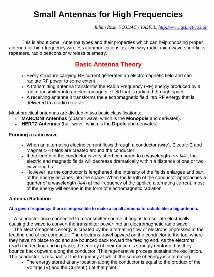
The Radiated Field is divided in three distinctive regions:

Reactive Near-Field is the region close to the antenna where the Electric-E and Magnetic-H fields are not orthogonal and anything within this region which couple with the antenna will distort the radiated pattern. In this region Antenna Gain is not a meaningful parameter.

Radiating Near-Field (transition region or Fresnel region) is the region between near and far field. In this region the antenna pattern is taking shape but is not fully formed. In this region Antenna Gain will vary with distance.

Far-Field (Fraunhofer region) is defined as that region of the field where the angular field distribution is essentially independent of the distance from the antenna. In this region Antenna Gain is constant with distance.

where and

Antenna Radiated Field Regions

Radiation Patterns

The radio signals radiated by an antenna form an electromagnetic field with a definite pattern, depending on the type of antenna used. This radiation pattern shows the antenna’s directional characteristics. The pattern is usually distorted by nearby obstructions.

The Directivity of an antenna is a measure of the antenna’s ability to focus the energy in one or more specific directions.

For example a vertical monopole antenna radiates energy equally in all azimuth directions

(omnidirectional) and a horizontal dipole antenna is mainly bidirectional. The maximum directivity of an antenna depends upon its physical size compared to wavelength.

The ratio between the amounts of energy propagated in particular directions and the energy that would be propagated if the antenna were not directional is known as Antenna Gain.

The Antenna Gain is constant if the antenna is used either for transmitting or receiving.

Measuring the radiated field of the antenna at one frequency, we can determine the radiation characteristics and the directivity gain of the antenna in a given direction.

The directivity gain is equal to the power gain in the absence of conduction loss in the antenna structure.

Ground losses affect radiation patterns and cause high signal losses for some frequencies. Such losses can be greatly reduced if a good conducting ground is provided in the vicinity of the antenna.

To achieve an antenna gain higher than normal, we must sacrifice the bandwidth under the most favorable conditions.

The Bandwidth is the antenna operating frequency band within which the antenna performs as desired. The bandwidth could be related to the antenna matching if its radiation patterns do not change within this frequency range. This is the case for small antennas where a fundamental limit relates bandwidth, size, and efficiency.

For a certain cut through the main beam of the antenna where most of the power is radiating, the angular distance between the half power points (-3dB) is defined as the Beamwidth.

There is no antenna able to radiate all the energy in one preferred direction. Some energy is inevitably radiated in other directions with lower levels than the main beam. These smaller peaks are referred to as Sidelobes, commonly specified in dB down from the main lobe.

The performance of an antenna designed on the free-space basis will be modified by the presence of physical objects in the neighborhood. Currents will be induced on the objects. They will give rise not only to an additional scattered radiation field, but also to a modification of the original current distribution on the antenna structure. Both, the gain and Q of the antenna will be changed from their unperturbed values.

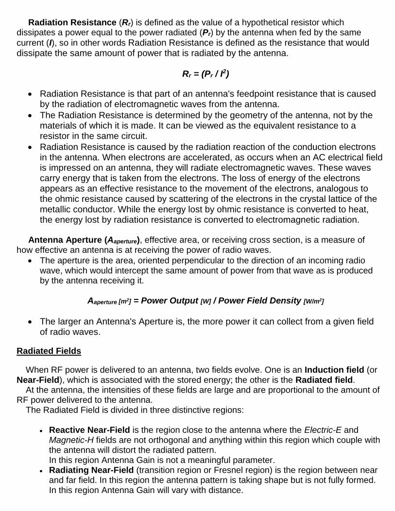
Antenna Pattern Convention Coordinates

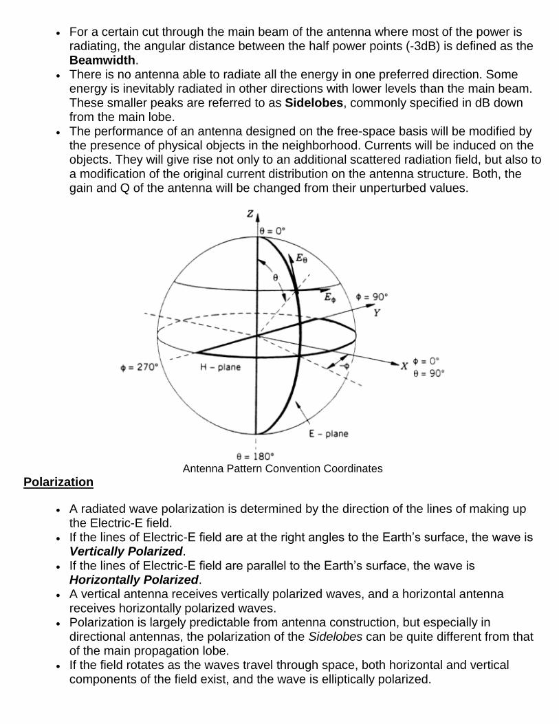
Polarization

A radiated wave polarization is determined by the direction of the lines of making up the Electric-E field.

If the lines of Electric-E field are at the right angles to the Earth’s surface, the wave is Vertically Polarized.

If the lines of Electric-E field are parallel to the Earth’s surface, the wave is Horizontally Polarized.

A vertical antenna receives vertically polarized waves, and a horizontal antenna receives horizontally polarized waves.

Polarization is largely predictable from antenna construction, but especially in directional antennas, the polarization of the Sidelobes can be quite different from that of the main propagation lobe.

If the field rotates as the waves travel through space, both horizontal and vertical components of the field exist, and the wave is elliptically polarized.

Circular Polarization describes a wave whose plane of polarization rotates through 360° as it progresses forward. The antenna continuously varies the Electric-E field of the radio wave through all possible values of its orientation with regard to the Earth’s surface. The rotation can be clockwise or counter-clockwise. Circular polarization occurs when equal magnitudes of vertically and horizontally polarized waves are combined with a phase difference of 90°.

Some antennas, such the helical antenna, produce circular polarizations. However, circular polarization can be generated from a linearly polarized antenna by feeding the antenna by two ports with equal magnitude and with a 90° phase difference between them.

Rotation in one direction or the other depends on the phase relationship.

"Hand rules" are used to describe the sense of circular polarization. The sense is defined by which hand would be used in order to point that thumb in the direction of propagation and point the fingers of the same hand in the direction of rotation of the Electric-E field vector. For example, if your thumb is pointed in the direction of propagation and the rotation is counterclockwise looking in the direction of travel, then you have Left Hand Circular Polarization (LHCP). If the rotation is clockwise then you have Right Hand Circular Polarization (RHCP).

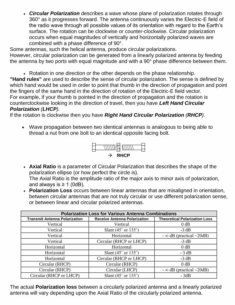
Wave propagation between two identical antennas is analogous to being able to

thread a nut from one bolt to an identical opposite facing bolt.

RHCP

Axial Ratio is a parameter of Circular Polarization that describes the shape of the polarization ellipse (or how perfect the circle is). The Axial Ratio is the amplitude ratio of the major axis to minor axis of polarization, and always is ≥ 1 (0dB).

Polarization Loss occurs between linear antennas that are misaligned in orientation, between circular antennas that are not truly circular or use different polarization sense, or between linear and circular polarized antennas.

Polarization Loss for Various Antenna Combinations Transmit Antenna Polarization Receive Antenna Polarization Theoretical Polarization Loss

Vertical Vertical 0 dB

Vertical Slant (45˚ or 135˚) -3 dB

Vertical Horizontal - ∞ dB (practical ~20dB)

Vertical Circular (RHCP or LHCP) -3 dB

Horizontal Horizontal 0 dB

Horizontal Slant (45˚ or 135˚) - 3 dB

Horizontal Circular (RHCP or LHCP) -3 dB

Circular (RHCP) Circular (RHCP) 0 dB

Circular (RHCP) Circular (LHCP) - ∞ dB (practical ~20dB)

Circular (RHCP or LHCP) Slant (45˚ or 135˚) - 3dB

The actual Polarization loss between a circularly polarized antenna and a linearly polarized antenna will vary depending upon the Axial Ratio of the circularly polarized antenna.

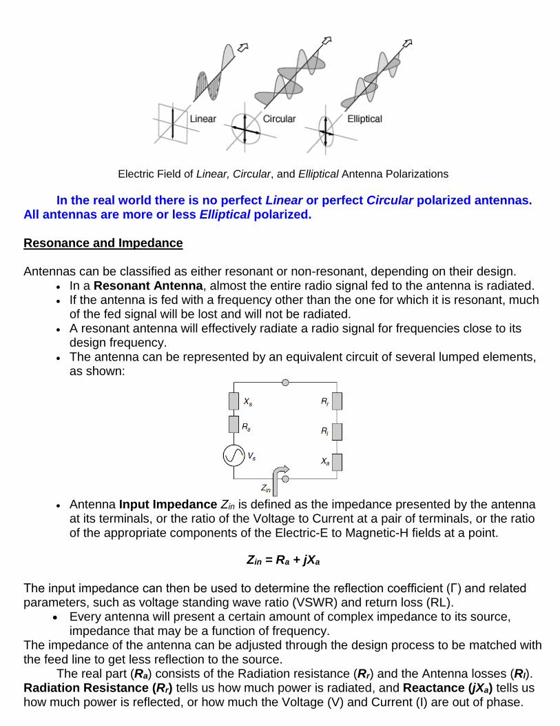
Electric Field of Linear, Circular, and Elliptical Antenna Polarizations

In the real world there is no perfect Linear or perfect Circular polarized antennas. All antennas are more or less Elliptical polarized. Resonance and Impedance

Antennas can be classified as either resonant or non-resonant, depending on their design.

In a Resonant Antenna, almost the entire radio signal fed to the antenna is radiated. If the antenna is fed with a frequency other than the one for which it is resonant, much

of the fed signal will be lost and will not be radiated. A resonant antenna will effectively radiate a radio signal for frequencies close to its

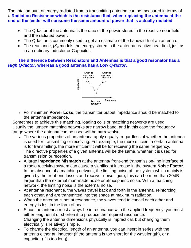
design frequency. The antenna can be represented by an equivalent circuit of several lumped elements,

as shown:

Antenna Input Impedance Zin is defined as the impedance presented by the antenna

at its terminals, or the ratio of the Voltage to Current at a pair of terminals, or the ratio of the appropriate components of the Electric-E to Magnetic-H fields at a point.

Zin = Ra + jXa

The input impedance can then be used to determine the reflection coefficient (Γ) and related parameters, such as voltage standing wave ratio (VSWR) and return loss (RL).

Every antenna will present a certain amount of complex impedance to its source, impedance that may be a function of frequency.

The impedance of the antenna can be adjusted through the design process to be matched with the feed line to get less reflection to the source.

The real part (Ra) consists of the Radiation resistance (Rr) and the Antenna losses (Rl). Radiation Resistance (Rr) tells us how much power is radiated, and Reactance (jXa) tells us how much power is reflected, or how much the Voltage (V) and Current (I) are out of phase.

The total amount of energy radiated from a transmitting antenna can be measured in terms of a Radiation Resistance which is the resistance that, when replacing the antenna at the end of the feeder will consume the same amount of power that is actually radiated.

The Q-factor of the antenna is the ratio of the power stored in the reactive near field and the radiated power.

The Q-factor is commonly used to get an estimate of the bandwidth of an antenna.

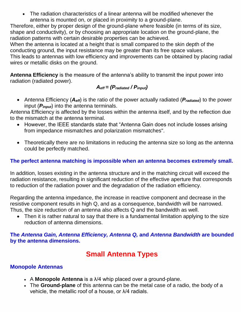
The reactance, jXa models the energy stored in the antenna reactive near field, just as in an ordinary Inductor or Capacitor.

The difference between Resonators and Antennas is that a good resonator has a High Q-factor, whereas a good antenna has a Low Q-factor.

For minimum Power Loss, the transmitter output impedance should be matched to the antenna impedance.

Sometimes to achieve this matching, loading coils or matching networks are used. Usually the lumped matching networks are narrow band, and in this case the frequency range where the antenna can be used will be narrow also.

The various properties of an antenna apply equally, regardless of whether the antenna is used for transmitting or receiving. For example, the more efficient a certain antenna is for transmitting, the more efficient it will be for receiving the same frequency. The directive properties of a given antenna will be the same, whether it is used for transmission or reception.

A large Impedance Mismatch at the antenna/ front-end transmission-line interface of a radio receiving system can cause a significant increase in the system Noise Factor. In the absence of a matching network, the limiting noise of the system which mainly is given by the front-end losses and receiver noise figure, this can be more than 20dB larger than the external man-made noise or atmospheric noise. With a matching network, the limiting noise is the external noise.

At antenna resonance, the waves travel back and forth in the antenna, reinforcing each other, and are transmitted into the space at maximum radiation.

When the antenna is not at resonance, the waves tend to cancel each other and energy is lost in the form of heat.

Since the antenna must always be in resonance with the applied frequency, you must either lengthen it or shorten it to produce the required resonance. Changing the antenna dimensions physically is impractical, but changing them electrically is relatively simple.

To change the electrical length of an antenna, you can insert in series with the antenna either an inductor (if the antenna is too short for the wavelength), or a capacitor (if is too long).

The radiation characteristics of a linear antenna will be modified whenever the antenna is mounted on, or placed in proximity to a ground-plane.

Therefore, either by proper design of the ground-plane where feasible (in terms of its size, shape and conductivity), or by choosing an appropriate location on the ground-plane, the radiation patterns with certain desirable properties can be achieved. When the antenna is located at a height that is small compared to the skin depth of the conducting ground, the input resistance may be greater than its free space values. This leads to antennas with low efficiency and improvements can be obtained by placing radial wires or metallic disks on the ground. Antenna Efficiency is the measure of the antenna’s ability to transmit the input power into radiation (radiated power).

Aeff = (Pradiated / Pinput)

Antenna Efficiency (Aeff) is the ratio of the power actually radiated (Pradiated) to the power input (Pinput) into the antenna terminals.

Antenna Efficiency is affected by the losses within the antenna itself, and by the reflection due to the mismatch at the antenna terminal.

However, the IEEE standards state that “Antenna Gain does not include losses arising from impedance mismatches and polarization mismatches".

Theoretically there are no limitations in reducing the antenna size so long as the antenna could be perfectly matched.

The perfect antenna matching is impossible when an antenna becomes extremely small. In addition, losses existing in the antenna structure and in the matching circuit will exceed the radiation resistance, resulting in significant reduction of the effective aperture that corresponds to reduction of the radiation power and the degradation of the radiation efficiency. Regarding the antenna impedance, the increase in reactive component and decrease in the resistive component results in high Q, and as a consequence, bandwidth will be narrowed. Thus, the size reduction of an antenna also affects Q and the bandwidth as well.

Then it is rather natural to say that there is a fundamental limitation applying to the size reduction of antenna dimensions.

The Antenna Gain, Antenna Efficiency, Antenna Q, and Antenna Bandwidth are bounded by the antenna dimensions.

Small Antenna Types

Monopole Antennas

A Monopole Antenna is a λ/4 whip placed over a ground-plane. The Ground-plane of this antenna can be the metal case of a radio, the body of a

vehicle, the metallic roof of a house, or λ/4 radials.

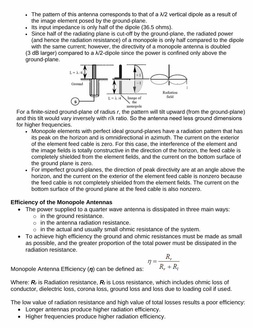
The pattern of this antenna corresponds to that of a λ/2 vertical dipole as a result of the image element posed by the ground-plane.

Its input impedance is only half of the dipole (36.5 ohms). Since half of the radiating plane is cut-off by the ground-plane, the radiated power

(and hence the radiation resistance) of a monopole is only half compared to the dipole with the same current; however, the directivity of a monopole antenna is doubled

(3 dB larger) compared to a λ/2-dipole since the power is confined only above the ground-plane.

For a finite-sized ground-plane of radius r, the pattern will tilt upward (from the ground-plane) and this tilt would vary inversely with r/λ ratio. So the antenna need less ground dimensions for higher frequencies.

Monopole elements with perfect ideal ground-planes have a radiation pattern that has its peak on the horizon and is omnidirectional in azimuth. The current on the exterior of the element feed cable is zero. For this case, the interference of the element and the image fields is totally constructive in the direction of the horizon, the feed cable is completely shielded from the element fields, and the current on the bottom surface of the ground plane is zero.

For imperfect ground-planes, the direction of peak directivity are at an angle above the horizon, and the current on the exterior of the element feed cable is nonzero because the feed cable is not completely shielded from the element fields. The current on the bottom surface of the ground plane at the feed cable is also nonzero.

Efficiency of the Monopole Antennas

The power supplied to a quarter wave antenna is dissipated in three main ways: o in the ground resistance. o in the antenna radiation resistance. o in the actual and usually small ohmic resistance of the system.

To achieve high efficiency the ground and ohmic resistances must be made as small as possible, and the greater proportion of the total power must be dissipated in the radiation resistance.

Monopole Antenna Efficiency (η) can be defined as:

Where: Rr is Radiation resistance, Rl is Loss resistance, which includes ohmic loss of conductor, dielectric loss, corona loss, ground loss and loss due to loading coil if used. The low value of radiation resistance and high value of total losses results a poor efficiency:

Longer antennas produce higher radiation efficiency.

Higher frequencies produce higher radiation efficiency.

Lower ground loss resistances produce higher radiation efficiency

Higher Q coils produces higher radiation efficiencies. High Q coils require a large conductor, air wound construction, large spacing between turns, and the best insulating material available.

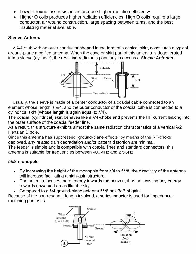
Sleeve Antenna

A λ/4-stub with an outer conductor shaped in the form of a conical skirt, constitutes a typical ground-plane modified antenna. When the cone or skirt part of this antenna is degenerated into a sleeve (cylinder), the resulting radiator is popularly known as a Sleeve Antenna.

Usually, the sleeve is made of a center conductor of a coaxial cable connected to an element whose length is λ/4, and the outer conductor of the coaxial cable is connected to a cylindrical skirt (whose length is again equal to λ/4). The coaxial (cylindrical) skirt behaves like a λ/4-choke and prevents the RF current leaking into the outer surface of the coaxial feeder line. As a result, this structure exhibits almost the same radiation characteristics of a vertical λ/2 Hertzian Dipole. Since this antenna has suppressed “ground-plane effects” by means of the RF-choke deployed, any related gain degradation and/or pattern distortion are minimal. The feeder is simple and is compatible with coaxial lines and standard connectors; this antenna is suitable for frequencies between 400MHz and 2.5GHz.

5λ/8 monopole

By increasing the height of the monopole from λ/4 to 5λ/8, the directivity of the antenna will increase facilitating a high-gain structure.

The antenna focuses more energy towards the horizon, thus not wasting any energy towards unwanted areas like the sky.

Compared to a λ/4 ground-plane antenna 5λ/8 has 3dB of gain. Because of the non-resonant length involved, a series inductor is used for impedance-matching purposes.

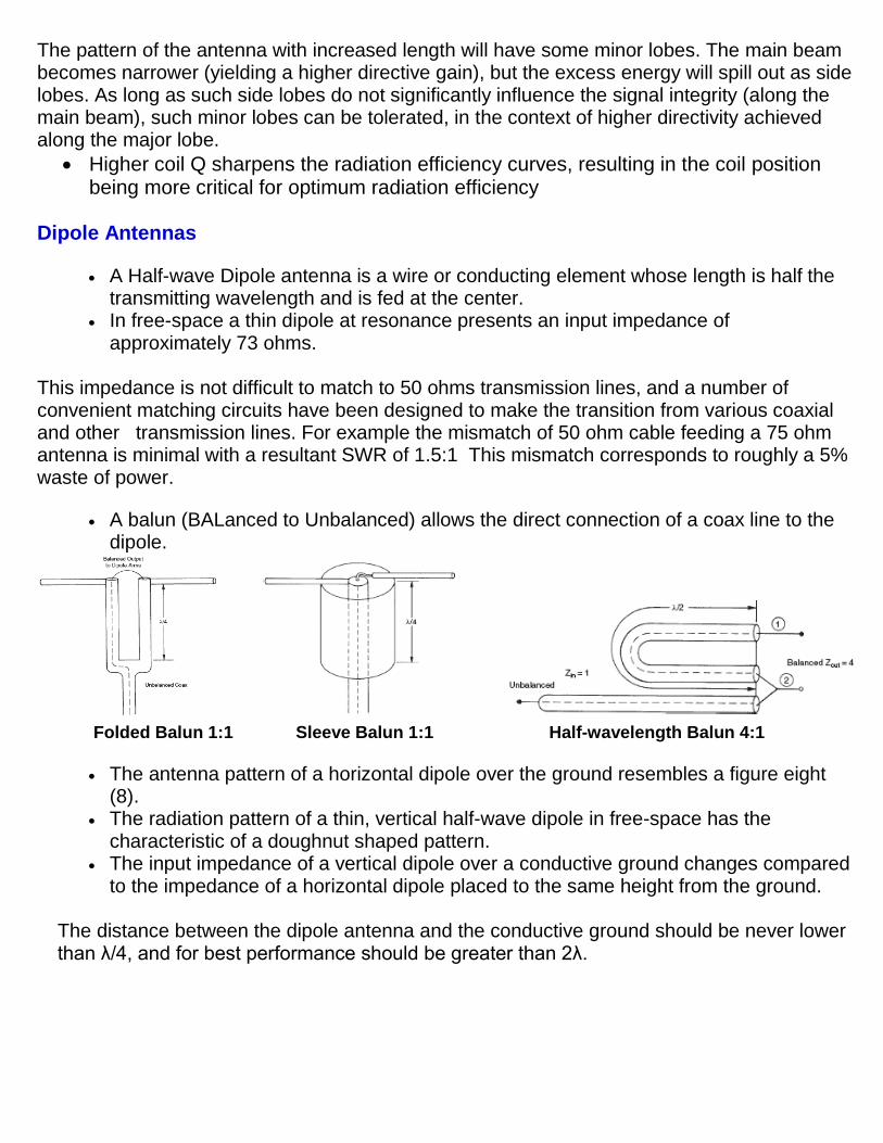
The pattern of the antenna with increased length will have some minor lobes. The main beam becomes narrower (yielding a higher directive gain), but the excess energy will spill out as side lobes. As long as such side lobes do not significantly influence the signal integrity (along the main beam), such minor lobes can be tolerated, in the context of higher directivity achieved along the major lobe.

Higher coil Q sharpens the radiation efficiency curves, resulting in the coil position being more critical for optimum radiation efficiency

Dipole Antennas

A Half-wave Dipole antenna is a wire or conducting element whose length is half the transmitting wavelength and is fed at the center.

In free-space a thin dipole at resonance presents an input impedance of approximately 73 ohms.

This impedance is not difficult to match to 50 ohms transmission lines, and a number of convenient matching circuits have been designed to make the transition from various coaxial and other transmission lines. For example the mismatch of 50 ohm cable feeding a 75 ohm antenna is minimal with a resultant SWR of 1.5:1 This mismatch corresponds to roughly a 5% waste of power.

A balun (BALanced to Unbalanced) allows the direct connection of a coax line to the dipole.

Folded Balun 1:1 Sleeve Balun 1:1 Half-wavelength Balun 4:1

The antenna pattern of a horizontal dipole over the ground resembles a figure eight (8).

The radiation pattern of a thin, vertical half-wave dipole in free-space has the characteristic of a doughnut shaped pattern.

The input impedance of a vertical dipole over a conductive ground changes compared to the impedance of a horizontal dipole placed to the same height from the ground.

The distance between the dipole antenna and the conductive ground should be never lower than λ/4, and for best performance should be greater than 2λ.

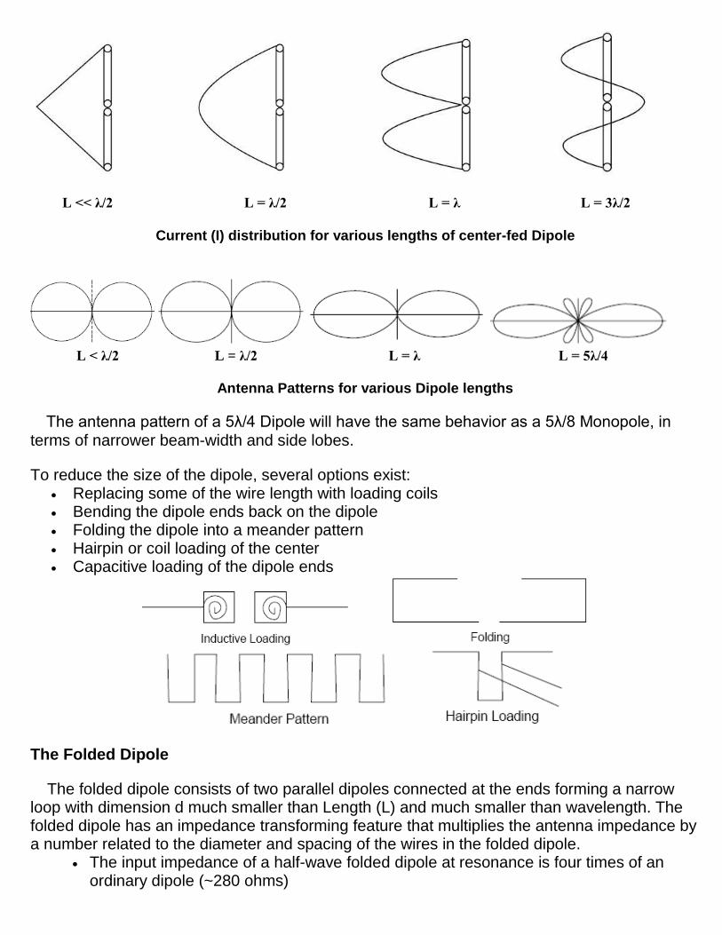
L << λ/2 L = λ/2 L = λ L = 3λ/2

Current (I) distribution for various lengths of center-fed Dipole

L < λ/2 L = λ/2 L = λ L = 5λ/4

Antenna Patterns for various Dipole lengths

The antenna pattern of a 5λ/4 Dipole will have the same behavior as a 5λ/8 Monopole, in terms of narrower beam-width and side lobes.

To reduce the size of the dipole, several options exist: Replacing some of the wire length with loading coils

Bending the dipole ends back on the dipole

Folding the dipole into a meander pattern

Hairpin or coil loading of the center Capacitive loading of the dipole ends

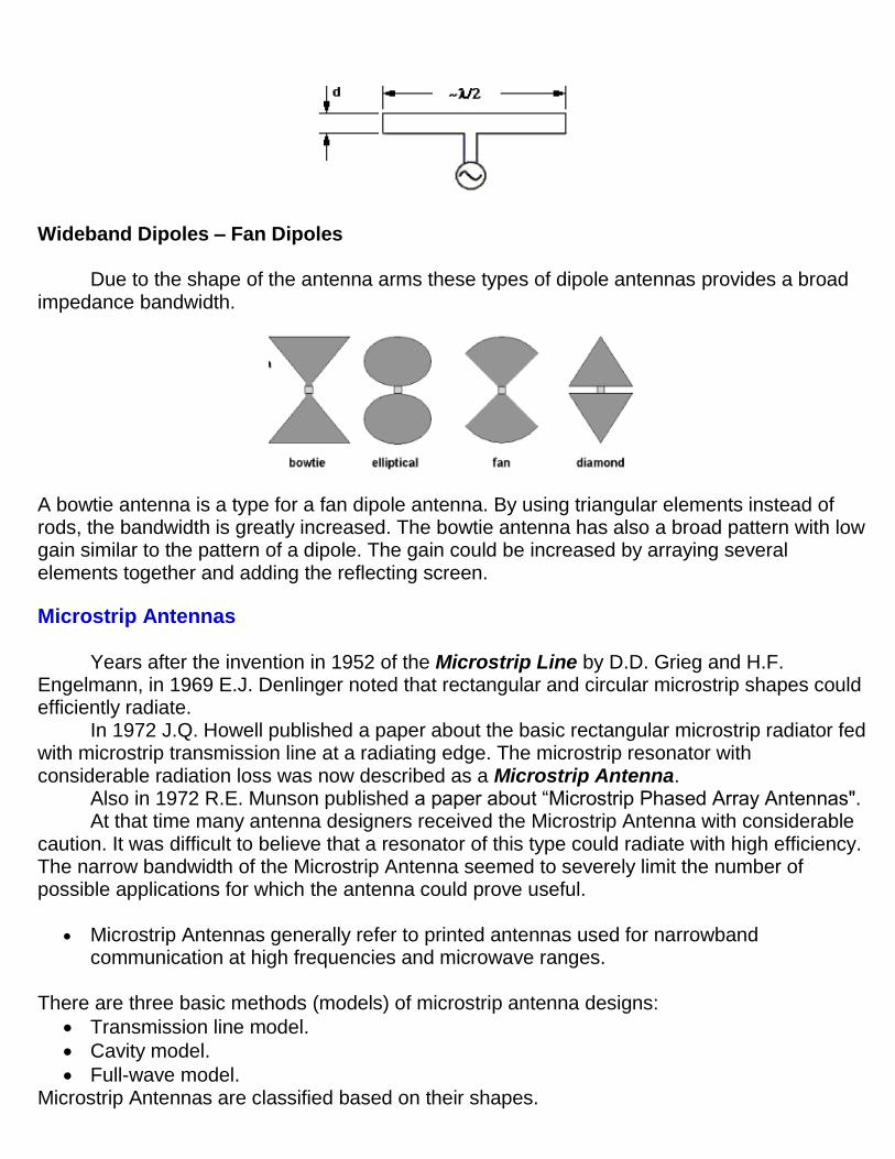
The Folded Dipole

The folded dipole consists of two parallel dipoles connected at the ends forming a narrow loop with dimension d much smaller than Length (L) and much smaller than wavelength. The folded dipole has an impedance transforming feature that multiplies the antenna impedance by a number related to the diameter and spacing of the wires in the folded dipole.

The input impedance of a half-wave folded dipole at resonance is four times of an ordinary dipole (~280 ohms)

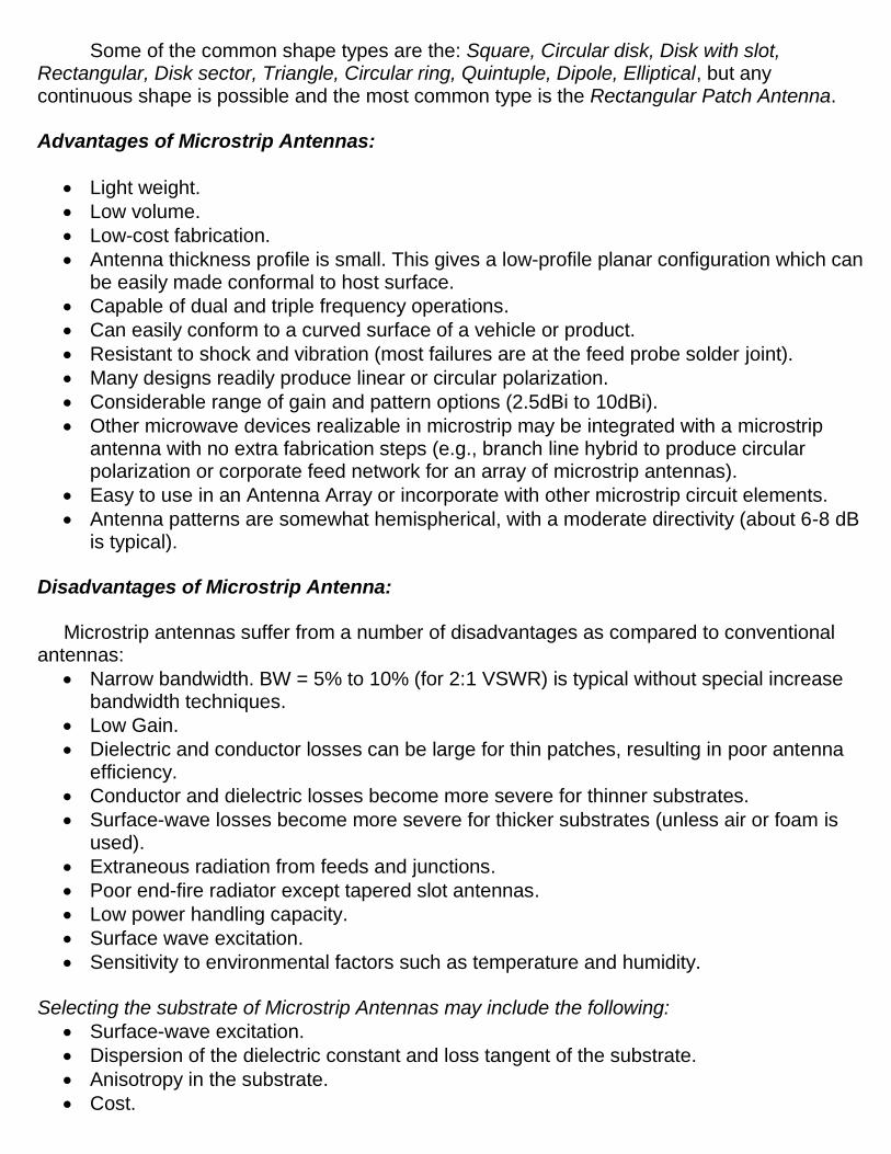
Wideband Dipoles – Fan Dipoles

Due to the shape of the antenna arms these types of dipole antennas provides a broad

impedance bandwidth.

A bowtie antenna is a type for a fan dipole antenna. By using triangular elements instead of rods, the bandwidth is greatly increased. The bowtie antenna has also a broad pattern with low gain similar to the pattern of a dipole. The gain could be increased by arraying several elements together and adding the reflecting screen.

Microstrip Antennas Years after the invention in 1952 of the Microstrip Line by D.D. Grieg and H.F.

Engelmann, in 1969 E.J. Denlinger noted that rectangular and circular microstrip shapes could efficiently radiate.

In 1972 J.Q. Howell published a paper about the basic rectangular microstrip radiator fed with microstrip transmission line at a radiating edge. The microstrip resonator with considerable radiation loss was now described as a Microstrip Antenna.

Also in 1972 R.E. Munson published a paper about “Microstrip Phased Array Antennas". At that time many antenna designers received the Microstrip Antenna with considerable

caution. It was difficult to believe that a resonator of this type could radiate with high efficiency. The narrow bandwidth of the Microstrip Antenna seemed to severely limit the number of possible applications for which the antenna could prove useful.

Microstrip Antennas generally refer to printed antennas used for narrowband

communication at high frequencies and microwave ranges. There are three basic methods (models) of microstrip antenna designs:

Transmission line model.

Cavity model.

Full-wave model. Microstrip Antennas are classified based on their shapes.

Some of the common shape types are the: Square, Circular disk, Disk with slot, Rectangular, Disk sector, Triangle, Circular ring, Quintuple, Dipole, Elliptical, but any continuous shape is possible and the most common type is the Rectangular Patch Antenna. Advantages of Microstrip Antennas:

Light weight.

Low volume.

Low-cost fabrication.

Antenna thickness profile is small. This gives a low-profile planar configuration which can be easily made conformal to host surface.

Capable of dual and triple frequency operations.

Can easily conform to a curved surface of a vehicle or product.

Resistant to shock and vibration (most failures are at the feed probe solder joint).

Many designs readily produce linear or circular polarization.

Considerable range of gain and pattern options (2.5dBi to 10dBi).

Other microwave devices realizable in microstrip may be integrated with a microstrip antenna with no extra fabrication steps (e.g., branch line hybrid to produce circular polarization or corporate feed network for an array of microstrip antennas).

Easy to use in an Antenna Array or incorporate with other microstrip circuit elements.

Antenna patterns are somewhat hemispherical, with a moderate directivity (about 6-8 dB is typical).

Disadvantages of Microstrip Antenna: Microstrip antennas suffer from a number of disadvantages as compared to conventional

antennas:

Narrow bandwidth. BW = 5% to 10% (for 2:1 VSWR) is typical without special increase bandwidth techniques.

Low Gain.

Dielectric and conductor losses can be large for thin patches, resulting in poor antenna efficiency.

Conductor and dielectric losses become more severe for thinner substrates.

Surface-wave losses become more severe for thicker substrates (unless air or foam is used).

Extraneous radiation from feeds and junctions.

Poor end-fire radiator except tapered slot antennas.

Low power handling capacity.

Surface wave excitation.

Sensitivity to environmental factors such as temperature and humidity. Selecting the substrate of Microstrip Antennas may include the following:

Surface-wave excitation.

Dispersion of the dielectric constant and loss tangent of the substrate.

Anisotropy in the substrate.

Cost.

Feeding Techniques for Microstrip Antennas Microstrip patch antennas can be fed by various methods, these methods can be classified

into two main categories namely:

Contacting methods

Non-contacting methods In the contacting method, the RF power is fed directly to the radiating patch using a connecting element such as a microstrip line, whereas in the non – contacting scheme, electromagnetic field coupling is done to transfer power between the microstrip line and the radiating patch. The four most popular feeding techniques used are:

Microstrip line.

Coaxial probe feed.

Aperture coupling.

Proximity coupling. While microstrip and coaxial probe feed are contacting schemes, aperture coupling and proximity coupling are non-contacting methods. Patch Antennas

The Patch Antenna is a popular resonant antenna used for narrow-band microwave wireless communications that require semispherical coverage. Some Patch Antennas avoid using a dielectric substrate and suspend a metal patch in the air above a ground plane using dielectric spacers; the resulting structure provides increased bandwidth.

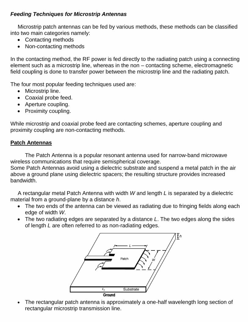
A rectangular metal Patch Antenna with width W and length L is separated by a dielectric material from a ground-plane by a distance h.

The two ends of the antenna can be viewed as radiating due to fringing fields along each edge of width W.

The two radiating edges are separated by a distance L. The two edges along the sides of length L are often referred to as non-radiating edges.

The rectangular patch antenna is approximately a one-half wavelength long section of

rectangular microstrip transmission line.

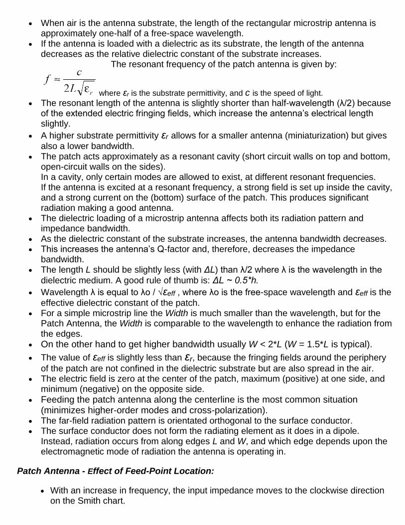
When air is the antenna substrate, the length of the rectangular microstrip antenna is approximately one-half of a free-space wavelength.

If the antenna is loaded with a dielectric as its substrate, the length of the antenna decreases as the relative dielectric constant of the substrate increases.

The resonant frequency of the patch antenna is given by:

where εr is the substrate permittivity, and c is the speed of light. The resonant length of the antenna is slightly shorter than half-wavelength (λ/2) because

of the extended electric fringing fields, which increase the antenna’s electrical length slightly.

A higher substrate permittivity εr allows for a smaller antenna (miniaturization) but gives

also a lower bandwidth. The patch acts approximately as a resonant cavity (short circuit walls on top and bottom,

open-circuit walls on the sides). In a cavity, only certain modes are allowed to exist, at different resonant frequencies. If the antenna is excited at a resonant frequency, a strong field is set up inside the cavity, and a strong current on the (bottom) surface of the patch. This produces significant radiation making a good antenna.

The dielectric loading of a microstrip antenna affects both its radiation pattern and impedance bandwidth.

As the dielectric constant of the substrate increases, the antenna bandwidth decreases. This increases the antenna’s Q-factor and, therefore, decreases the impedance

bandwidth. The length L should be slightly less (with ΔL) than λ/2 where λ is the wavelength in the

dielectric medium. A good rule of thumb is: ΔL ~ 0.5*h.

Wavelength λ is equal to λo / √εeff , where λo is the free-space wavelength and εeff is the

effective dielectric constant of the patch. For a simple microstrip line the Width is much smaller than the wavelength, but for the

Patch Antenna, the Width is comparable to the wavelength to enhance the radiation from the edges.

On the other hand to get higher bandwidth usually W < 2*L (W = 1.5*L is typical).

The value of εeff is slightly less than εr, because the fringing fields around the periphery

of the patch are not confined in the dielectric substrate but are also spread in the air. The electric field is zero at the center of the patch, maximum (positive) at one side, and

minimum (negative) on the opposite side.

Feeding the patch antenna along the centerline is the most common situation (minimizes higher-order modes and cross-polarization).

The far-field radiation pattern is orientated orthogonal to the surface conductor. The surface conductor does not form the radiating element as it does in a dipole.

Instead, radiation occurs from along edges L and W, and which edge depends upon the electromagnetic mode of radiation the antenna is operating in.

Patch Antenna - Effect of Feed-Point Location:

With an increase in frequency, the input impedance moves to the clockwise direction on the Smith chart.

The width W of the patch antenna has significant effect on the Input impedance, Bandwidth, and Gain of the antenna.

With an increase in W, the input impedance decreases, so the feed point is shifted toward the edge to obtain input resistance Rin in the range of 50 ohms to 65ohms.

Patch Antenna - Effect of the height h (substrate thickness):

With the increase in h, the fringing fields from the edges increase, this increases the extension in effective length L, however decreasing the resonance frequency.

The input impedance plot moves clockwise (i.e., an inductive shift occurs) due to the increase in the probe inductance of the coaxial feed.

The Bandwidth of patch antenna increases with height. The directivity of the antenna increases marginally with increasing height because the

effective aperture area is increased marginally due to increase in ΔL. Generally, the antenna efficiency increases with an increase in the substrate thickness

initially due to the increase in the radiated power, but thereafter, it starts decreasing because of the higher cross-polar level and excitation of the surface wave.

The surface waves get excited and travel along the dielectric substrate (i.e., between the ground plane and the dielectric-to air interface due to total internal reflection). When these waves reach the edges of the substrate, they are reflected, scattered, and diffracted causing a reduction in gain and an increase in end-fire radiation and cross-polar levels.

The excitation of surface waves is a function of εr and h. The power loss in the surface

waves increases with an increase in the normalized thickness h/λo of the substrate.

Patch Antenna - Effect of substrate Dielectric Constant εr:

Decreasing substrate Dielectric Constant (εr) the Bandwidth of the patch increases.

Patch Antenna - Effect of Finite Ground Plane:

In practice, the size of the patch ground plane is finite. When the size of the ground plane is greater than the patch dimensions by

approximately six times the substrate thickness all around the periphery, the results are similar to that of the infinite ground plane.

If the loss in the dielectric material increases the input impedance Zin of the patch antenna decreases.

Patch Antenna Bandwidth: Patch Antenna Bandwidth can be increased using the following techniques:

Using thick and low permittivity substrates. For example by using a thick foam substrate

with εr = 1.2, a bandwidth of about 10% of resonant frequency can be achieved.

Introducing closely spaced parasitic patches on the same layer of the fed patch (provides 15% BW).

Using a stacked parasitic patch (multilayer, BW reaches 20%).

Introducing a U-shaped slot in the patch (to achieve 30% BW).

Aperture coupling (provides 10% BW and high back-lobe radiation).

Aperture-coupled stacked patches (40–50% BW achievable).

Using L-probe coupling.

The bandwidth is directly proportional to the width W, and a good rule is: W=1.5*L.

Patch Antenna Resonant Input Resistance

The resonant input resistance is almost independent of the substrate thickness h.

The resonant input resistance is proportional to εr, and is strong depending by εr if the

patch is fed at the edge. In this case for a typical patch, the input resistance may be about 100-200 ohms.

The resonant input resistance is directly controlled by the location of the fed point. (maximum at edges, and zero at center of patch).

Patch Antenna is usually fed along the centerline (y = W / 2) to maintain symmetry and thus minimize excitation of undesirable modes.

Patch Antenna Radiation Efficiency

Radiation efficiency is the ratio of power radiated into space, to the total input power. The radiation efficiency is less than 100% due to:

- conductor loss - dielectric loss - surface-wave power

Conductor and dielectric loss is more important for thinner substrates.

Conductor loss increases with frequency (proportional to f ½ due to the skin effect).

Conductor loss is usually more important than dielectric loss.

Surface-wave power is more important for thicker substrates or for higher substrate permittivity.

The surface-wave power can be minimized by using a foam substrate. For a foam substrate, higher radiation efficiency is obtained by making the substrate thicker (minimizing the conductor and dielectric losses). The thicker the better.

Patch Antenna Radiation Pattern

The E-plane pattern is typically broader than the H-plane pattern.

The truncation of the ground plane will cause edge diffraction, which tends to degrade the pattern by introducing rippling in the forward direction back-radiation.

The directivity is fairly insensitive to the substrate thickness.

The directivity is higher for lower permittivity, because the patch is larger. Patch Antenna Feeding Methods

Coaxial Feed

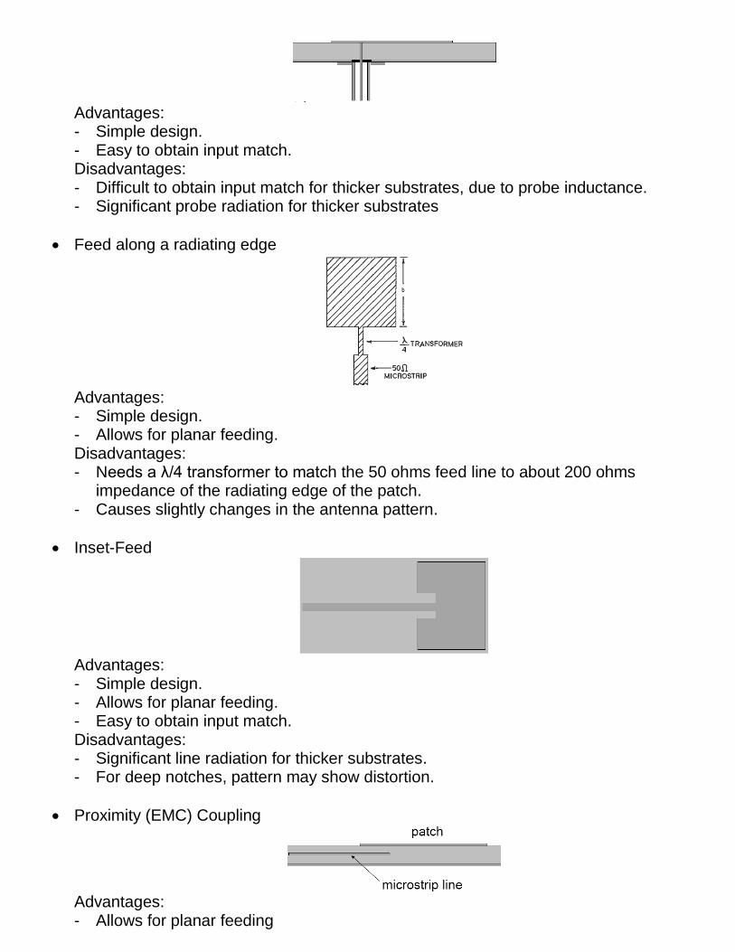
Advantages: - Simple design. - Easy to obtain input match. Disadvantages: - Difficult to obtain input match for thicker substrates, due to probe inductance. - Significant probe radiation for thicker substrates

Feed along a radiating edge

Advantages: - Simple design. - Allows for planar feeding. Disadvantages: - Needs a λ/4 transformer to match the 50 ohms feed line to about 200 ohms

impedance of the radiating edge of the patch. - Causes slightly changes in the antenna pattern.

Inset-Feed

Advantages: - Simple design. - Allows for planar feeding. - Easy to obtain input match. Disadvantages: - Significant line radiation for thicker substrates. - For deep notches, pattern may show distortion.

Proximity (EMC) Coupling

Advantages: - Allows for planar feeding

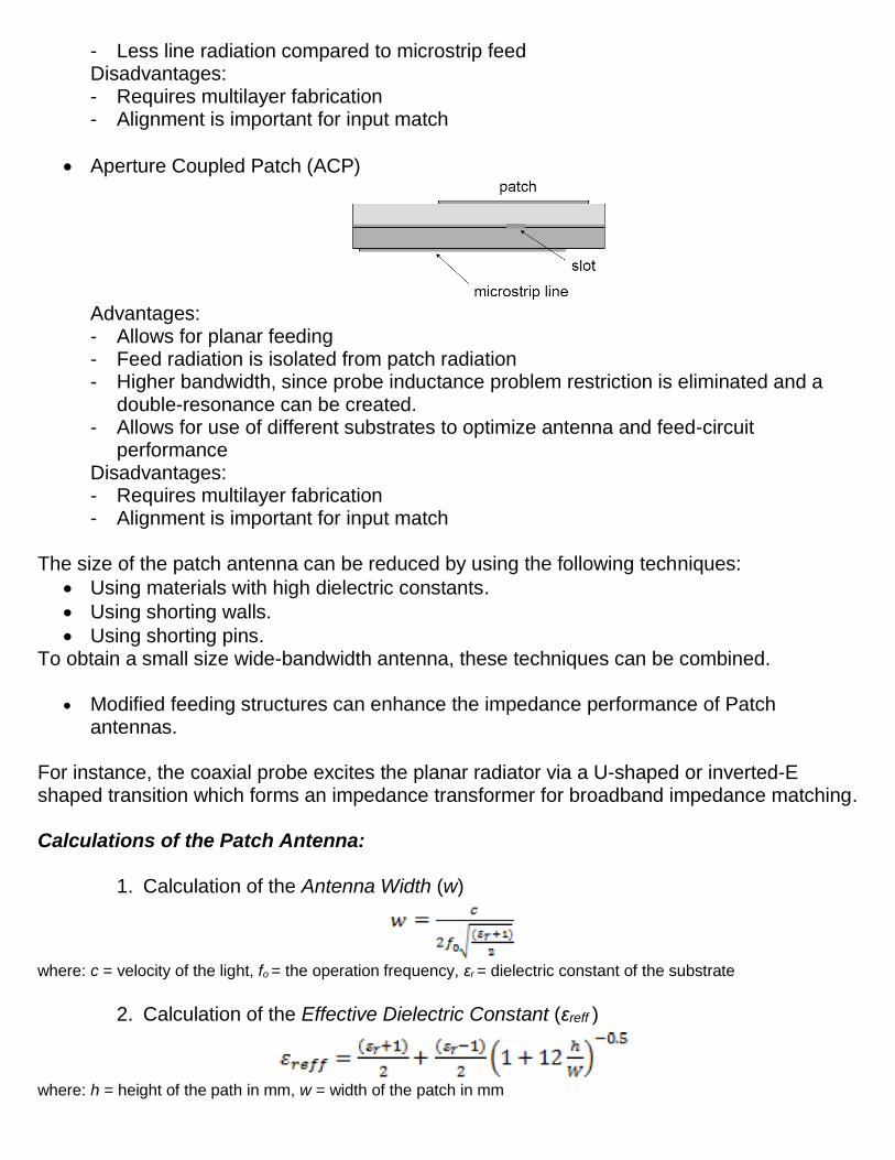
- Less line radiation compared to microstrip feed Disadvantages: - Requires multilayer fabrication - Alignment is important for input match

Aperture Coupled Patch (ACP)

Advantages: - Allows for planar feeding - Feed radiation is isolated from patch radiation - Higher bandwidth, since probe inductance problem restriction is eliminated and a

double-resonance can be created. - Allows for use of different substrates to optimize antenna and feed-circuit

performance Disadvantages: - Requires multilayer fabrication - Alignment is important for input match

The size of the patch antenna can be reduced by using the following techniques:

Using materials with high dielectric constants.

Using shorting walls.

Using shorting pins. To obtain a small size wide-bandwidth antenna, these techniques can be combined.

Modified feeding structures can enhance the impedance performance of Patch antennas.

For instance, the coaxial probe excites the planar radiator via a U-shaped or inverted-E shaped transition which forms an impedance transformer for broadband impedance matching. Calculations of the Patch Antenna:

1. Calculation of the Antenna Width (w)

where: c = velocity of the light, fo = the operation frequency, εr = dielectric constant of the substrate

2. Calculation of the Effective Dielectric Constant (εreff )

where: h = height of the path in mm, w = width of the patch in mm

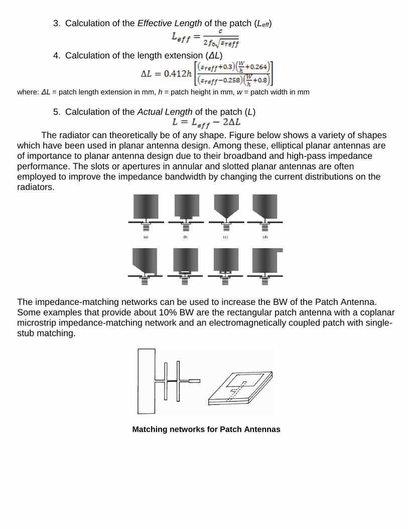
3. Calculation of the Effective Length of the patch (Leff)

4. Calculation of the length extension (ΔL)

where: ΔL = patch length extension in mm, h = patch height in mm, w = patch width in mm

5. Calculation of the Actual Length of the patch (L)

The radiator can theoretically be of any shape. Figure below shows a variety of shapes

which have been used in planar antenna design. Among these, elliptical planar antennas are of importance to planar antenna design due to their broadband and high-pass impedance performance. The slots or apertures in annular and slotted planar antennas are often employed to improve the impedance bandwidth by changing the current distributions on the radiators.

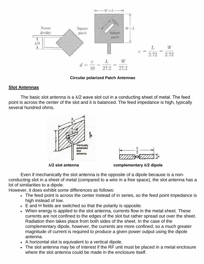
The impedance-matching networks can be used to increase the BW of the Patch Antenna. Some examples that provide about 10% BW are the rectangular patch antenna with a coplanar microstrip impedance-matching network and an electromagnetically coupled patch with single-stub matching.

Matching networks for Patch Antennas

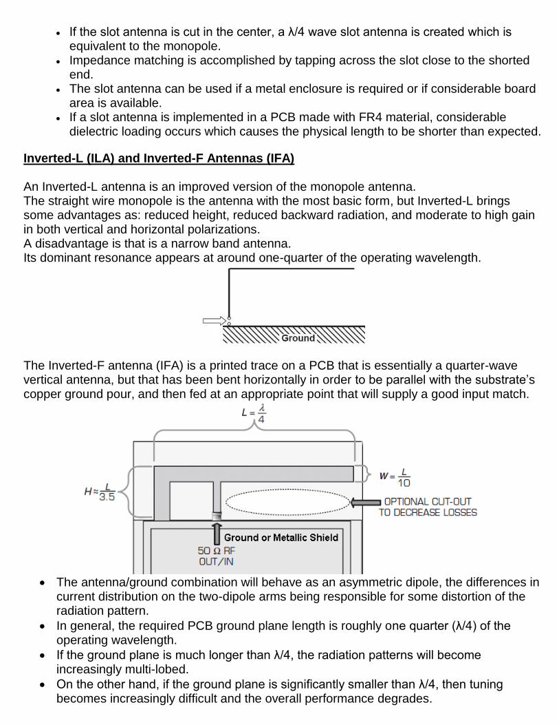
Circular polarized Patch Antennas

Slot Antennas

The basic slot antenna is a λ/2 wave slot cut in a conducting sheet of metal. The feed point is across the center of the slot and it is balanced. The feed impedance is high, typically several hundred ohms.

λ/2 slot antenna complementary λ/2 dipole

Even if mechanically the slot antenna is the opposite of a dipole because is a non-conducting slot in a sheet of metal (compared to a wire in a free space), the slot antenna has a lot of similarities to a dipole. However, it does exhibit some differences as follows:

The feed point is across the center instead of in series, so the feed point impedance is high instead of low.

E and H fields are switched so that the polarity is opposite. When energy is applied to the slot antenna, currents flow in the metal sheet. These

currents are not confined to the edges of the slot but rather spread out over the sheet. Radiation then takes place from both sides of the sheet. In the case of the complementary dipole, however, the currents are more confined; so a much greater magnitude of current is required to produce a given power output using the dipole antenna.

A horizontal slot is equivalent to a vertical dipole. The slot antenna may be of interest if the RF unit must be placed in a metal enclosure

where the slot antenna could be made in the enclosure itself.

If the slot antenna is cut in the center, a λ/4 wave slot antenna is created which is equivalent to the monopole.

Impedance matching is accomplished by tapping across the slot close to the shorted end.

The slot antenna can be used if a metal enclosure is required or if considerable board area is available.

If a slot antenna is implemented in a PCB made with FR4 material, considerable dielectric loading occurs which causes the physical length to be shorter than expected.

Inverted-L (ILA) and Inverted-F Antennas (IFA) An Inverted-L antenna is an improved version of the monopole antenna. The straight wire monopole is the antenna with the most basic form, but Inverted-L brings some advantages as: reduced height, reduced backward radiation, and moderate to high gain in both vertical and horizontal polarizations. A disadvantage is that is a narrow band antenna. Its dominant resonance appears at around one-quarter of the operating wavelength.

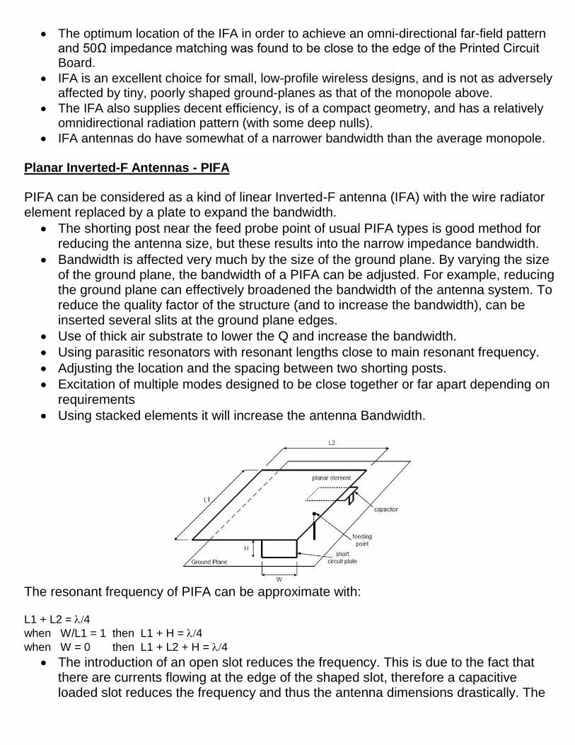
The Inverted-F antenna (IFA) is a printed trace on a PCB that is essentially a quarter-wave vertical antenna, but that has been bent horizontally in order to be parallel with the substrate’s copper ground pour, and then fed at an appropriate point that will supply a good input match.

The antenna/ground combination will behave as an asymmetric dipole, the differences in

current distribution on the two-dipole arms being responsible for some distortion of the radiation pattern.

In general, the required PCB ground plane length is roughly one quarter (λ/4) of the operating wavelength.

If the ground plane is much longer than λ/4, the radiation patterns will become increasingly multi-lobed.

On the other hand, if the ground plane is significantly smaller than λ/4, then tuning becomes increasingly difficult and the overall performance degrades.

The optimum location of the IFA in order to achieve an omni-directional far-field pattern and 50Ω impedance matching was found to be close to the edge of the Printed Circuit Board.

IFA is an excellent choice for small, low-profile wireless designs, and is not as adversely affected by tiny, poorly shaped ground-planes as that of the monopole above.

The IFA also supplies decent efficiency, is of a compact geometry, and has a relatively omnidirectional radiation pattern (with some deep nulls).

IFA antennas do have somewhat of a narrower bandwidth than the average monopole. Planar Inverted-F Antennas - PIFA

PIFA can be considered as a kind of linear Inverted-F antenna (IFA) with the wire radiator element replaced by a plate to expand the bandwidth.

The shorting post near the feed probe point of usual PIFA types is good method for reducing the antenna size, but these results into the narrow impedance bandwidth.

Bandwidth is affected very much by the size of the ground plane. By varying the size of the ground plane, the bandwidth of a PIFA can be adjusted. For example, reducing the ground plane can effectively broadened the bandwidth of the antenna system. To reduce the quality factor of the structure (and to increase the bandwidth), can be inserted several slits at the ground plane edges.

Use of thick air substrate to lower the Q and increase the bandwidth.

Using parasitic resonators with resonant lengths close to main resonant frequency.

Adjusting the location and the spacing between two shorting posts.

Excitation of multiple modes designed to be close together or far apart depending on requirements

Using stacked elements it will increase the antenna Bandwidth.

The resonant frequency of PIFA can be approximate with:

L1 + L2 = /4

when W/L1 = 1 then L1 + H = /4

when W = 0 then L1 + L2 + H = /4

The introduction of an open slot reduces the frequency. This is due to the fact that there are currents flowing at the edge of the shaped slot, therefore a capacitive loaded slot reduces the frequency and thus the antenna dimensions drastically. The

same principle of making slots in the planar element can be applied for dual-frequency operation as well.

Changes in the width of the planar element can also affect the determination of the resonant frequency.

The width of the short circuit plate of the PIFA plays a very important role in governing its resonant frequency. Resonant frequency decreases with the decrease in short circuit plate width, W.

Unlike micro-strip antennas that are conventionally made of half wavelength dimensions, PIFA’s are made of just quarter-wavelength.

Analyzing the resonant frequency and the bandwidth characteristics of the antenna can be easily done by determining the site of the feed point, which the minimum reflection coefficient is to be obtained.

The impedance matching of the PIFA is obtained by positioning of the single feed and the shorting pin within the shaped slot, and by optimizing the space between feed and shorting pins.

The main idea designing a PIFA is to don’t use any extra lumped components for matching network, and thus avoid any losses due to that.

The radiation pattern of the PIFA is the relative distribution of radiated power as a function of direction in space.

In the usual case the radiation pattern is determined in the far-field region and is represented as a function of directional coordinates. Radiation properties include power flux density, field strength, phase, and polarization.

PIFA has very large current flows on the undersurface of the planar element and the ground plane compared to the field on the upper surface of the element. Due to this behavior PIFA is one of the best candidate when is talking about the influence of the external objects that affect the antenna characteristics (e.g. mobile operator’s hand/head).

PIFA surface current distribution varies for different widths of short-circuit plates. The maximum current distribution is close to the short pin and decrease away from it.

Impedance bandwidth of PIFA is inversely proportional to the quality factor Q that is defined for a resonator.

Substrates with high dielectric constant (Er) tend to store energy more than radiate it. This is equivalent by modeling the PIFA as a lossy capacitor with high Er, thus leading to high Q value and obviously reducing the bandwidth. Similarly when the substrate thickness is increased the inverse proportionality of thickness to the capacitance decreases the energy stored in the PIFA and the Q factor decreases also.

In summary, the increase in height and decrease of Er can be used to increase the bandwidth of the PIFA.

The efficiency of PIFA in its environment is reduced by all losses suffered by it, including: ohmic losses, mismatch losses, feedline transmission losses, edge power losses, external parasitic resonances, etc.

The PIFA itself is an antenna of inherently low gain and narrow band, say about 1%–2% when the antenna is placed on an infinite or comparable size of ground-plane.

However, a PIFA installed on a finite size ground-plane, for example that in a mobile phone terminal, exhibits higher gain and wider bandwidth than the antenna in free space.

This improvement is a result caused by the assistance of the ground-plane, on which the radiation current excited by the PIFA flows, and the performance of the entire antenna (gain and bandwidth) that is the PIFA plus the ground-plane, is improved.

Loop Antennas The Loop Antenna refers to a radiating element made of a coil of one or more turns.

The dissipative resistance in the loop, ignoring dielectric loss, is depended by the Loop Perimeter, the conductor Width/Thickness, the Magnetic Permeability µ, the Conductivity σ, and by the Frequency.

The loop's inductance is determined by the Circumference, the Enclosed Area, the conductor Width/Thickness, and the Magnetic Permeability.

Loop antennas can be divided in three groups:

1. Full-wave Loop antenna

2. Half-wave Loop antenna

3. Series-loaded, Small-loop antenna

1. The Full-wave Loop is approximately one (λ) wavelength in circumference. Resonance is obtained when the loop is slightly longer than one (λ) wavelength. The full wave loop can be thought of as two end-connected dipoles. Like any other loop, the shape of the full wave loop is not critical, but efficiency is determined mainly by the enclosed area. The feed impedance is somewhat higher than the half-wave loop antenna (approximately 120 Ohms).

The main advantage of the full-wave loop antenna is it does not have the air gap in the loop, which is very sensitive to load and PCB capacitance spread.

2. The Half-wave Loop consists of a loop approximately λ/2 wavelength in circumference with a gap cut in the ring. It is very similar to a half-wave dipole that has been folded into a ring and most of the information about the dipole applies to the half-wave loop. Because the ends are very close together, there exists some capacitive loading, and resonance is obtained at a somewhat smaller circumference than expected. The feed-point impedance is also somewhat lower than the usual dipole, but all the usual feeding techniques can be applied to the half-wave loop.

The half-wave loop is popular at lower frequencies but at higher frequencies, the tuning capacitance across the gap becomes very small and critical.

3. The circumference of a Small-Loop antenna is smaller than λ/2. The radiation resistance of the Small-Loop antenna is extremely small. In addition, the resistance arising from the dissipative losses can be more than ten times the radiation resistance. The radiation resistance of a small-loop can be increased increasing the number of turns, or inserting within its circumference a ferrite core with high permeability.

The radiated resistance (Rr) of a Small-Loop antenna can be calculated with:

Rr = 31171*(A/λ2)2 where the number 31171 is 320*π4, and A (loop area) and λ (wavelength) in the same units. For example a λ/10 diameter loop would have A = π(λ/20)2, and the radiation resistance (Rr) is found to be 1.92 ohms. The actual feedpoint impedance will include the resistive loss of the conductor (with skin effect), plus the inductance of the loop, which will have a result in range of 3.0 +j800 ohms.

The radiation pattern and gain are similar to the λ/10 short dipole.

Current distribution is nearly uniform on a Small-Loop antenna. Typically, a Small-Loop antenna may be able to radiate only a few percent of the power that

comes from the transmitter. The radiation pattern of a Small-Loop antenna is identical with that of a small dipole.

In the near-field the loop stores most of its energy in a Magnetic-H field and the short dipole stores its near-field energy in an Electric-E field, but the waves radiated by each have the same E/H; they are equally electric and magnetic.

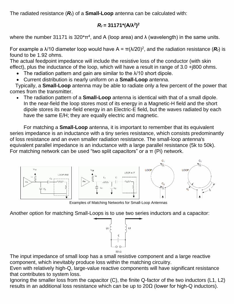
For matching a Small-Loop antenna, it is important to remember that its equivalent

series impedance is an inductance with a tiny series resistance, which consists predominantly of loss resistance and an even smaller radiation resistance. The small-loop antenna's equivalent parallel impedance is an inductance with a large parallel resistance (5k to 50k). For matching network can be used “two split capacitors” or a π (Pi) network.

Examples of Matching Networks for Small-Loop Antennas

Another option for matching Small-Loops is to use two series inductors and a capacitor:

The input impedance of small loop has a small resistive component and a large reactive component, which inevitably produce loss within the matching circuitry. Even with relatively high-Q, large-value reactive components will have significant resistance that contributes to system loss. Ignoring the smaller loss from the capacitor (C), the finite Q-factor of the two inductors (L1, L2) results in an additional loss resistance which can be up to 20Ω (lower for high-Q inductors).

Helical Antenna

A conducting wire wound in the form of a screw thread can form a Helix Antenna. Usually the Helix Antenna uses a ground plane with different forms.

The diameter of the ground plane should be greater than 3λ/4. In general the Helix is connected to the center conductor of a coaxial transmission line and the outer conductor of the line is attached to the ground plane.

The parameters which characterize a Helix antenna are: N = the number of turns, D = the diameter of the Helix, S = the spacing between each turn, L = total Length of the antenna

α = the Pitch angle which is the angle formed by the line tangent to the helix wire and a plane perpendicular to the helix axis.

When α = 0˚, then the winding is flattened and the helix reduces to a loop antenna of N turns. When α = 90˚, then the helix reduces to a linear wire. When 0˚ < α < 90˚, then a true helix is formed.

The radiation characteristics of the antenna can be varied by controlling the size of its geometrical properties compared to the wavelength.

The input impedance is critically dependent upon pitch angle and the size of the conducting wire, especially near the feed point.

The main modes of operation of the Helix antenna are Normal mode (broadside) and the Axial mode (endfire).

Normal mode

In the Normal mode of operation the field radiated by the Helix is maximum in a perpendicular plane to the Helix axis.

To achieve the Normal mode of operation the dimensions of Helix are usually small compared to wavelength (D<<λ and L<<λ).

In the Normal mode it can be thought that the Helix consists of N small loops and N short dipoles connected together in series.

Since in the Normal mode the Helix dimensions are small, the current through its length can be assumed to be constant and its relative far-field pattern to be independent of the number of loops and short dipoles.

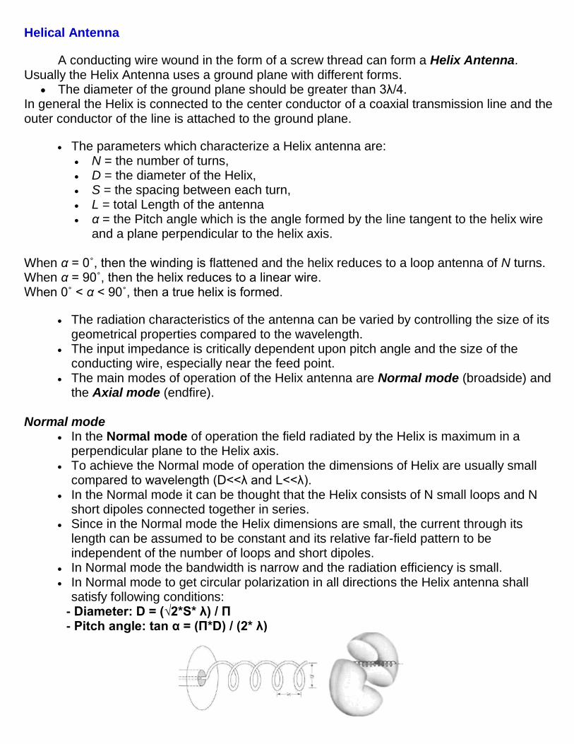
In Normal mode the bandwidth is narrow and the radiation efficiency is small. In Normal mode to get circular polarization in all directions the Helix antenna shall

satisfy following conditions: - Diameter: D = (√2*S* λ) / Π - Pitch angle: tan α = (Π*D) / (2* λ)

Axial mode

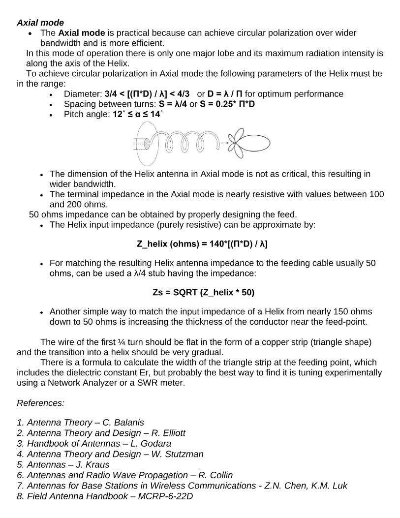
The Axial mode is practical because can achieve circular polarization over wider bandwidth and is more efficient.

In this mode of operation there is only one major lobe and its maximum radiation intensity is along the axis of the Helix. To achieve circular polarization in Axial mode the following parameters of the Helix must be

in the range: Diameter: 3/4 < [(Π*D) / λ] < 4/3 or D = λ / Π for optimum performance

Spacing between turns: S = λ/4 or S = 0.25* Π*D

Pitch angle: 12˚ ≤ α ≤ 14˚

The dimension of the Helix antenna in Axial mode is not as critical, this resulting in

wider bandwidth. The terminal impedance in the Axial mode is nearly resistive with values between 100

and 200 ohms. 50 ohms impedance can be obtained by properly designing the feed.

The Helix input impedance (purely resistive) can be approximate by:

Z_helix (ohms) = 140*[(Π*D) / λ]

For matching the resulting Helix antenna impedance to the feeding cable usually 50 ohms, can be used a λ/4 stub having the impedance:

Zs = SQRT (Z_helix * 50)

Another simple way to match the input impedance of a Helix from nearly 150 ohms down to 50 ohms is increasing the thickness of the conductor near the feed-point.

The wire of the first ¼ turn should be flat in the form of a copper strip (triangle shape)

and the transition into a helix should be very gradual. There is a formula to calculate the width of the triangle strip at the feeding point, which

includes the dielectric constant Er, but probably the best way to find it is tuning experimentally using a Network Analyzer or a SWR meter. References:

1. Antenna Theory – C. Balanis 2. Antenna Theory and Design – R. Elliott 3. Handbook of Antennas – L. Godara 4. Antenna Theory and Design – W. Stutzman 5. Antennas – J. Kraus 6. Antennas and Radio Wave Propagation – R. Collin 7. Antennas for Base Stations in Wireless Communications - Z.N. Chen, K.M. Luk 8. Field Antenna Handbook – MCRP-6-22D

9. Monopole Antennas – M. Weiner 10. Complete Wireless Design – C. Sayre 11. Loop Antennas – G.Smith 12. High Frequency Electronics Magazine (2002 – 2013) 13. International Journal of Emerging Technology and Advanced Engineering 14. Planar Antennas for Wireless Communications – Wong 15. Microwave Engineering – Pozar 16. PIFA for Mobile Phones – Haridas 17. Microstrip and Printed Antenna Design - R.Bancroft 18. Overview of Microstrip Antennas - D.Jackson 19. Modern Small Antennas - Fujimoto, Morishita

home http://www.qsl.net/va3iul/