slowness: an objective for spike-timing–dependent …sprekeler/data/paper/sprekeler... · one...

Slowness: An Objective forSpike-Timing–Dependent Plasticity?Henning Sprekeler

*, Christian Michaelis, Laurenz Wiskott

Institute for Theoretical Biology, Humboldt-Universitat zu Berlin, Berlin, Germany

Our nervous system can efficiently recognize objects in spite of changes in contextual variables such as perspective orlighting conditions. Several lines of research have proposed that this ability for invariant recognition is learned byexploiting the fact that object identities typically vary more slowly in time than contextual variables or noise. Here, westudy the question of how this ‘‘temporal stability’’ or ‘‘slowness’’ approach can be implemented within the limits ofbiologically realistic spike-based learning rules. We first show that slow feature analysis, an algorithm that is based onslowness, can be implemented in linear continuous model neurons by means of a modified Hebbian learning rule. Thisapproach provides a link to the trace rule, which is another implementation of slowness learning. Then, we showanalytically that for linear Poisson neurons, slowness learning can be implemented by spike-timing–dependentplasticity (STDP) with a specific learning window. By studying the learning dynamics of STDP, we show that forfunctional interpretations of STDP, it is not the learning window alone that is relevant but rather the convolution ofthe learning window with the postsynaptic potential. We then derive STDP learning windows that implement slowfeature analysis and the ‘‘trace rule.’’ The resulting learning windows are compatible with physiological data both inshape and timescale. Moreover, our analysis shows that the learning window can be split into two functionallydifferent components that are sensitive to reversible and irreversible aspects of the input statistics, respectively. Thetheory indicates that irreversible input statistics are not in favor of stable weight distributions but may generateoscillatory weight dynamics. Our analysis offers a novel interpretation for the functional role of STDP in physiologicalneurons.

Citation: Sprekeler H, Michaelis C, Wiskott L (2007) Slowness: An objective for spike-timing–dependent plasticity? PLoS Comput Biol 3(6): e112. doi:10.1371/journal.pcbi.0030112

Introduction

The ability to recognize objects in spite of possible changesin position, lighting conditions, or perspective is doubtlesslyan advantage in everyday life. However, our brain usuallyperforms this task with such astonishing ease that we areseldom aware of the complexity this recognition problemcomprises. On the level of primary sensory signals (e.g., lightthat stimulates a single retinal receptor), even small changesin the position of the object to be recognized may lead tovastly different stimuli. Our brain thus has to somehowidentify rather different stimuli as representations of thesame underlying cause, i.e., it has to develop an internalrepresentation that is invariant to irrelevant changes of thestimulus. The work presented here is motivated by thequestion of how such invariant representations could beestablished.

Because of the limited amount of information in thegenome as well as the apparent flexibility of the neuraldevelopment in different environments, it seems unlikely thatthe information needed to form invariant representations isalready there at the beginning of individual development.Some information must be gathered from the sensory inputexperienced during interaction with the environment; it hasto be learned. As this learning process is likely to be at leastpartially unsupervised, the brain requires a heuristics as towhat stimuli should be classified as being the same.

One possible indicator for stimuli to represent the sameobject is temporal proximity. A scene that the eye views isvery unlikely to change completely from one moment to thenext. Rather, there is a good chance that an object that can be

seen now will also be present at the next instant of time. Thisimplies that invariant representations should remain stableover time, that is, they should vary slowly. Inverting thisreasoning, a sensory system that adapts to its sensory input inorder to extract slowly varying aspects may succeed inlearning invariant representations. This ‘‘slowness’’ or ‘‘tem-poral stability’’ principle is the basis of a whole class oflearning algorithms [1–7]. Most applications of this approachhave focused on models of the visual system, in particular onthe self-organized formation of complex cell receptive fieldsin the primary visual cortex [8,9].For clarity, we will focus on one of these algorithms, slow

feature analysis (SFA; [10]); a close link to the so-called ‘‘tracerule’’ will arise naturally. The goal of SFA is the following:given a multidimensional input signal x(t) and a finite-dimensional function space F, find the input–output func-tion g1(x) in F that generates the most slowly varying outputsignal y1(t)¼ g1(x(t)). It is important to note that the functiong1(x) is required to be an instantaneous function of the input

Editor: Lyle Graham, UFR Biomedicale de l’Universite Rene Descart, France

Received December 27, 2006; Accepted May 4, 2007; Published June 29, 2007

Copyright: � 2007 Sprekeler et al. This is an open-access article distributed underthe terms of the Creative Commons Attribution License, which permits unrestricteduse, distribution, and reproduction in any medium, provided the original authorand source are credited.

Abbreviations: EPSP, excitatory postsynaptic potential; LTD, long-term depression;LTP, long-term potentiation; SFA, slow feature analysis; STDP, spike-timing–dependent plasticity

* To whom correspondence should be addressed. E-mail: [email protected]

PLoS Computational Biology | www.ploscompbiol.org June 2007 | Volume 3 | Issue 6 | e1121136

signal. Otherwise, slow output signals could be generated bylow-pass filtering the input signal. As the goal of the slownessprinciple is to detect slowly varying features of the inputsignals, a mere low-pass filter would certainly generate slowoutput signals, but it would not serve the purpose.

As a measure of slowness, or rather ‘‘fastness,’’ SFA uses thevariance of the time derivative,h _yðtÞ2it, which is the objectivefunction to be minimized. Here, h�it denotes temporalaveraging. For mathematical convenience and to avoid thetrivial constant response, y1(t)¼ const, a zero-mean, and unitvariance constraint are imposed. Furthermore, it is possibleto find a second function g2(x) extracting y2(t) ¼ g2(x(t)) thatagain minimizes the given objective under the constraint ofbeing uncorrelated with y1(t), a third one uncorrelated withboth y1(t) and y2(t), and so on, thereby generating a set of slowfeatures of the input ordered by the degree of slowness.However, in this paper, we will consider just one singleoutput unit.

SFA has been applied to the learning of translation,rotation, and other invariances in a model of the visualsystem [10], and it has been shown that when applied to imagesequences generated from static natural images, SFA learnsfunctions that reproduce a wide range of features of complexcells in primary visual cortex [8]. Iteration of the sameprinciple in a hierarchical model in combination with asparseness objective has been used to model the self-organized formation of spatial representations resemblingplace cells as found in the hippocampal formation of rodents[11] (see [12] for related work).

These findings suggest that on an abstract level SFA reflectscertain aspects of cortical information processing. However,SFA as a technical algorithm is biologically rather implau-sible. There is in particular one step in its canonicalformulation that seems especially odd compared with whatneurons are normally thought to do. In this step theeigenvector that corresponds to the smallest eigenvalue ofthe covariance matrix of the time derivative of some

multidimensional signal is extracted. The aim of this paperis to show how this kind of computation can be realized in aspiking model neuron.In the following, we will first consider a continuous model

neuron and demonstrate that a modified Hebbian learningrule enables the neuron to learn the slowest (in the sense ofSFA) linear combination of its inputs. Apart from providingthe basis for the analysis of the spiking model, this sectionreveals a mathematical link between SFA and the tracelearning rule, another implementation of the slownessprinciple. We then examine if these findings also hold for aspiking model neuron, and find that for a linear Poissonneuron, spike-timing–dependent plasticity (STDP) can beinterpreted as an implementation of the slowness principle.

Results

Continuous Model NeuronLinear model neuron and basic assumptions. First, consider

a linear continuous model neuron with an input–outputfunction given by

aoutðtÞ ¼Xni¼1

wia ini ðtÞ; ð1Þ

with aini ðtÞ indicating the input signals, wi the weights, and aout

the output signal. For mathematical convenience, let aini ðtÞandaout (t) be defined on the interval t 2 [�‘, ‘] but differ fromzero only on [0,T], which could be the lifetime of the system.We assume that the input is approximately whitened on anysufficiently large interval [ta,tb] � [0,T] (i.e., each input signalhas approximately zero mean and unit variance and isuncorrelated with other input signals):

Ztbta

a ini ðtÞdt’ 0 ðzero meanÞ; ð2Þ

1Tab

Ztbta

a ini ðtÞ

2 dt’ 1 ðunit varianceÞ; ð3Þ

Ztbta

a ini ðtÞ a in

j 6¼i ðtÞdt’ 0 ðdecorrelationÞ: ð4Þ

This can be achieved by a normalization and decorrelationstep of the units projecting to the considered unit.Furthermore, we assume that the output is normalized tounit variance, which for whitened input means that theweight vector is normalized to length 1. In an online learningrule, this could be implemented by either an activity-dependent or a weight-dependent normalization term. Thus,for the output signal we have:

Ztbta

aoutðtÞdt ’ð1;2Þ

0; ðzero meanÞ ð5Þ


Author Summary

Neurons interact by exchanging information via small connectionsites, so-called synapses. Interestingly, the efficiency of synapses intransmitting neuronal signals is not static, but changes dynamicallydepending on the signals that the associated neurons emit. Asneurons receive thousands of synaptic input signals, they can thus‘‘choose’’ the input signals they are interested in by adjusting theirsynapses accordingly. This adaptation mechanism, known assynaptic plasticity, has long been hypothesized to form the neuronalcorrelate of learning. It raises a difficult question: what aspects of theinput signals are the neurons interested in, given that theadaptation of the synapses follows a certain mechanistic rule? Weaddress this question for spike-timing–dependent plasticity, a typeof synaptic plasticity that has raised a lot of interest in the lastdecade. We show that under certain assumptions regardingneuronal information transmission, spike-timing–dependent plasti-city focuses on aspects of the input signals that vary slowly in time.This relates spike-timing–dependent plasticity to a class of abstractlearning rules that were previously proposed as a means of learningto recognize objects in spite of contextual changes such as size orposition. Based on this link, we propose a novel functionalinterpretation of spike-timing–dependent plasticity.

Slowness Principle and STDP

1Tab

Ztbta

aoutðtÞ2 dt ’ð1;3ÞXn

i¼1w 2i :¼ 1: ðunit varianceÞ ð6Þ

In the following, we will often consider filtered signals.Therefore, we introduce abbreviations for the convolution f�gand the cross-correlation f * g of two functions f(t) and g(t):

Convolution: ½ f � g�ðtÞ :¼Z‘�‘

f ðsÞgðt� sÞ ds; ð7Þ

Cross - correlation: ½ f � g�ðtÞ :¼Z‘�‘

f ðsÞgðtþ sÞ ds: ð8Þ

For convenience, we will often use windowed signals,indicated by a hat

sðtÞ ¼ sðtÞ for t 2 ½ta; tb�0 otherwise

;

�ð9Þ

which allows us to replace the integration of a signal s(t) over[ta,tb] by an integration of s(t) over [�‘, ‘]. We assume that theinterval [ta,tb] is long compared to the width of the filters. Inthis case, effects from the integration boundaries arenegligible, and we have

Ztbta

½ f � s�ðtÞ hðtÞ dt’Z‘�‘

½ f � s�ðtÞhðtÞ dt: ð10Þ

Similar considerations hold for the cross-correlation (Equa-tion 8).

Since convolution and cross-correlation are convenientlytreated in Fourier space, we repeat the definition of theFourier transform Fs(m) and the power spectrum Ps(m) of asignal s(t).

Fourier transform: sðtÞ ¼:

Z‘�‘

F sðmÞ e2pimt dm; ð11Þ

Power spectrum: PsðmÞ :¼ F sðmÞ �F sðmÞ: ð12Þ

Throughout the paper, we make the assumption that inputsignals (and hence also the output signals) do not havesignificant power above some reasonable frequency mmax.

Reformulation of the slowness objective. SFA is based onthe minimization of the second moment of the time

derivative,Z

_aoutðtÞ2 dt. Even though there are neurons with

transient responses to changes in the input, we believe itwould be more plausible if we could derive an SFA-learningrule that does not depend on the time derivative, because itmight be difficult to extract, especially for spiking neurons. Itis indeed possible to replace the time derivative by a low-passfiltering as follows:

minimizeZ‘�‘

_aoutðtÞ2 dt ð13Þ

¼Z‘�‘

P _aoutðmÞdt ðbecause of Parseval0s theoremÞ ð14Þ

¼ 4p2Z‘�‘

m2Paout ðmÞdm ðsince F _sðmÞ ¼ 2pimF sðmÞÞ ð15Þ

, maximizeZ‘�‘

�m2PaoutðmÞdm ð16Þ

, maximizeZ‘�‘

ðm2max � m2ÞPaout ðmÞdm

sinceZ ‘

�‘

Paout mð Þdm ¼Z ‘

�‘

aout tð Þ2 dt ’6ð Þconst

! ð17Þ

¼Z‘�‘

maxð0; ðm2max � m2ÞÞPaoutðmÞdm

ðsince PaoutðmÞ ¼ 0 for jmj.mmax by assumptionÞ

ð18Þ

¼Z‘�‘

P fSFAðmÞPaout ðmÞdm ð19Þ

with fSFAðtÞ defined such that P fSFAðmÞ ¼ maxð0; ðm2max � m2ÞÞÞ�

ð20Þ

¼Z‘�‘

½ fSFA � aout�ðtÞ2 dt: ð21Þ

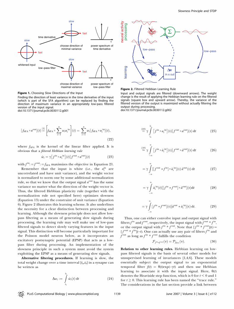
Thus, SFA can be achieved either by minimizing the varianceof the time derivative of the output signal or by maximizingthe variance of the appropriately filtered output signal.Figure 1 provides an intuition for this alternative. The filterfSFA is obviously a low-pass filter, as one would expect, with am2max � m2 power spectrum below the limiting frequency mmax.Because the phases are not determined, further assumptionsare required to fully determine an SFA filter. However, wewill proceed without defining a concrete filter, since it is notrequired for the considerations below.Hebbian learning on filtered signals. It is known that

standard Hebbian learning under the constraint of a unitweight vector applied to a linear unit maximizes the varianceof the output signal. We have seen in the previous section thatSFA can be reformulated as a maximization problem for thevariance of the low-pass filtered output signal. To achievethis, we simply apply Hebbian learning to the filtered inputand output signals, instead of to the original signals.Consider a hypothetical unit that receives low-pass filtered

inputs and, therefore, because of the linearity of the unit andthe filtering, generates a low-pass filtered output



½ fSFA � aout�ðtÞ ¼ð1Þ

fSFA �Xni¼1

wia ini

" #ðtÞ ¼

Xni¼1

wi½ fSFA � a ini �ðtÞ;

ð22Þ

where fSFA is the kernel of the linear filter applied. It isobvious that a filtered Hebbian learning rule

_wi ¼ c f in � aini

� �ðtÞ½ f out � aout�ðtÞ ð23Þ

with f in:¼ f out:¼ fSFA maximizes the objective in Equation 21.Remember that the input is white (i.e., the aini are

uncorrelated and have unit variance), and the weight vectoris normalized to norm one by some additional normalizationrule, so that we know that the output signal aout has the samevariance no matter what the direction of the weight vector is.Thus, the filtered Hebbian plasticity rule (together with thenormalization rule not specified here) optimizes slowness(Equation 13) under the constraint of unit variance (Equation6). Figure 2 illustrates this learning scheme. It also underlinesthe necessity for a clear distinction between processing andlearning. Although the slowness principle does not allow low-pass filtering as a means of generating slow signals duringprocessing, the learning rule may well make use of low-passfiltered signals to detect slowly varying features in the inputsignal. This distinction will become particularly important forthe Poisson model neuron below, as it incorporates anexcitatory postsynaptic potential (EPSP) that acts as a low-pass filter during processing. An implementation of theslowness principle in such a system must avoid the systemexploiting the EPSP as a means of generating slow signals.

Alternative filtering procedures. If learning is slow, thetotal weight change over a time interval [ta,tb] in a synapse canbe written as

Dwi :¼Ztbta

_wiðtÞdt ð24Þ

¼ð23Þ cZtbta

f in � aini

� �ðtÞ½ f out � aout�ðtÞdt ð25Þ

’ð10Þ

cZ‘�‘

f in � aini

� �ðtÞ½ f out � aout�ðtÞdt ð26Þ

¼ cZ‘�‘

½½ f out � f in� � a ini �ðtÞ aoutðtÞdt ð27Þ

¼ cZ‘�‘

a ini ðtÞ½½ f in � f out� � a

out�ðtÞdt ð28Þ

¼ cZ‘�‘

½ f in � f out�ðtÞ½aout � a ini �ðtÞdt: ð29Þ

Thus, one can either convolve input and output signal withfilters f in and f out, respectively, the input signal with f out * f in,or the output signal with f in * f out. Note that [ f in * f out](t) ¼[ f out * f in](�t). One can actually use any pair of filters f in andf out as long as f in * f out fulfills the condition

F f in�f outðmÞ ¼ P fSFAðmÞ: ð30Þ

Relation to other learning rules. Hebbian learning on low-pass filtered signals is the basis of several other models forunsupervised learning of invariances [1,4,6]. These modelsessentially subject the output signal to an exponentialtemporal filter f(t) ¼ h(t)exp(�ct) and then use Hebbianlearning to associate it with the input signal. Here, h(t)denotes the Heaviside step function, which is 0 for t , 0 and 1for t � 0. This learning rule has been named the ‘‘trace rule.’’The considerations in the last section provide a link between

Figure 1. Choosing Slow Directions of the Input

Finding the direction of least variance in the time derivative of the input(which is part of the SFA algorithm) can be replaced by finding thedirection of maximum variance in an appropriately low-pass filteredversion of the input signal.doi:10.1371/journal.pcbi.0030112.g001

Figure 2. Filtered Hebbian Learning Rule

Input and output signals are filtered (downward arrows). The weightchange is the result of applying the Hebbian learning rule on the filteredsignals (square box and upward arrow). Thereby, the variance of thefiltered version of the output is maximized without actually filtering theoutput during processing.doi:10.1371/journal.pcbi.0030112.g002



this approach and ours. We simply have to replace f in with ad-function and f out with f(t). Equation 29 then takes the form

Dwi ¼ cXj

Z ‘

�‘

f ðtÞ½a inj � a in

i �ðtÞdt� �

wj; ð31Þ

since the output signal aout ¼P

j wja inj is a linear function of

the input (see Equation 1). In the previously mentionedapplications of the trace rule, the statistics of the inputsignals were always reversible, so we will assume that allcorrelation functions ½a in

i � a inj �ðtÞ are symmetric in time. This

implies that only the symmetric component of f(t) is relevantfor learning:

f symðtÞ :¼ 12ð f ðtÞ þ f ð�tÞÞ ¼ c

2expð�cjtjÞ: ð32Þ

It is easy to show that the learning rule in Equation 31 can beinterpreted as a gradient ascent on the following objectivefunction:

W ¼Z‘�‘

f symðtÞ½aout � aout�ðtÞdt ð33Þ

¼Z‘�‘

F f symðmÞP aoutðmÞdm: ð34Þ

By comparison with Equation 19, it becomes clear that thetrace rule implements a very similar objective as our model.The only difference is that the power spectrum in Equation20 is replaced by the Fourier transform of the filter f sym. Notethat in order to be able to interpret W as an objectivefunction, it should be real-valued. The replacement of f withf sym ensures that F f sym is real-valued and symmetric, so W isreal-valued as well. The Fourier transform of f sym is given by

F f symðmÞ ¼c

c2 þ ð2pmÞ2: ð35Þ

This shows that the only difference between the trace ruleand our model lies in the choice of the power spectrum forthe low-pass filter. While we are using a parabolic powerspectrum with a cutoff (Equation 20), the trace rule uses apower spectrum with the shape of a Cauchy function(Equation 35).

From this perspective, one can interpret SFA as a quadraticapproximation of the trace rule. To what extent thisapproximation is valid depends on the power spectra of theinput signals. If most of the input power is concentrated atlow frequencies, where the power spectrum resembles aparabola, the learning rules can be expected to learn verysimilar weight vectors. In fact, any Hebbian learning rule thatleads to an objective function of the shape of Equation 19with a low-pass filtering spectrum in the place of PfSFAessentially implements the slowness principle, as amongsignals with the same variance, it will favor slower ones.

Spiking Model NeuronReal neurons do not transmit information via a continuous

stream of analog values like the model neuron considered inthe previous section, but rather emit action potentials thatcarry information by means of their rate and probably also by

their exact timing, a fact we will not consider here. How canthe model developed so far be mapped onto this scenario?The linear Poisson neuron. Again, we restrict our analysis

to a simple case by modeling the spike-train signals byinhomogeneous Poisson processes. Note that at this point, werestrict our analysis to a rate code, thus neglecting possiblecoding paradigms that rely on precise timing of spikes.To generate the input spike trains, we first add sufficiently

large constants c ini to the continuous and zero-mean signalsa ini ðtÞ to turn them into strictly positive signals that can beinterpreted as rates

r ini ðtÞ :¼ c ini þ a in

i ðtÞ: ð36Þ

The constants c ini represent mean firing rates, which aremodulated by the input signals a in

i . From the input ratesr ini ðtÞ, we then derive inhomogeneous Poisson spike trainsS ini ðtÞ drawn from ensembles E in

i such that

hS ini ðtÞiE in

i¼ r in

i ðtÞ; ð37Þ

where h�iE ini

denotes the average over the ensemble E ini .

The output rate is modeled as a weighted sum over theinput spike trains convolved with an EPSP e(t) plus a baselinefiring rate r0, which ensures that the output firing rateremains positive. This is necessary as we allow inhibitorysynapses (i.e., negative weights).

mðtÞ :¼ r0 þXni¼1

wi e � Sini

� �ðtÞ ð38Þ

Note that in this scheme, the EPSP reflects the change inthe postsynaptic firing probability due to a presynaptic spikerather than a change in the membrane potential. Ideally, itincludes all delay effects in neuronal transmission.The output of this spiking neuron is yet another

inhomogeneous Poisson spike train Sout(t) drawn from anensemble Eout, given a realization of the input spike trains S in

isuch that

hSoutðtÞiEout jfS ini g¼ mðtÞ: ð39Þ

It should be noted that not only is the output spike trainSout(t) stochastic in this model, but also the underlying outputrate m(t), which is a function of the stochastic variables SiðtÞand generally differs for each realization of the input. This isthe reason why the input and output spike trains are notstatistically independent. However, due to the linearity of themodel neuron, the output rate is still simply

routðtÞ ¼ hSoutðtÞiE ini ;Eout ð40Þ

¼ð39;38;37Þr0 þ

Xni¼1

wi e � rini

� �ðtÞ ð41Þ

¼ð36Þ r0 þXni¼1

wic ini

Z‘�‘

eðtÞdt

|fflfflfflfflfflfflfflfflfflfflfflfflfflfflfflfflfflfflfflffl{zfflfflfflfflfflfflfflfflfflfflfflfflfflfflfflfflfflfflfflffl}¼:cout

þXni¼1

wi e � aini

� �ðtÞ ð42Þ

¼ cout þ e �Xni¼1

wia ini

" #ðtÞ ð43Þ



¼ð1Þ cout þ ½e � aout�ðtÞ; ð44Þ

and the joint firing rate is

r in;outi ðt; t9Þ :¼ hS in

i ðtÞ Soutðt9ÞiE ini ;Eout ð45Þ

¼ r ini ðtÞroutðt9Þ þ wieðt9�tÞr in

i ðtÞ ðsee ½13�Þ: ð46Þ

The first term would result also from a rate model, whilethe second term captures the statistical dependenciesbetween input and output spike trains mediated by thesynaptic weights wi and the EPSP e(t).

STDP can perform SFA. In this section, we will demonstratethat in an ensemble-averaged sense it is possible to generatethe same weight distribution as in the continuous model bymeans of an STDP rule with a specific learning window.

Synaptic plasticity that depends on the temporal order ofpre- and postsynaptic spikes has been found in a number ofneuronal systems [14–18], and has raised a lot of interestamong modelers [19,20] (for a review, see [21]). Typically,synapses undergo long-term potentiation (LTP) if a presy-naptic spike precedes a postsynaptic spike within a timescaleof tens of milliseconds and long-term depression (LTD) forthe opposite temporal order. Assuming that the change insynaptic efficacy occurs on a slower timescale than the typicalinterspike interval, the STDP weight dynamics can bemodeled as

Dwi ¼ cXm in

i

a

Xmout

b

Wðtinia � toutb Þ: ð47Þ

Here, tinia denotes the spike times of the presynapticspikes at synapse i and toutb denotes the postsynaptic spiketimes. W(t) is the learning window that determines if and towhat extent the synapse is potentiated or depressed by asingle spike pair. The convention is such that negativearguments t in W(t) correspond to the situation where thepresynaptic spike precedes the postsynaptic spike. min

i andmout are the numbers of pre- and postsynaptic spikesoccurring in the time interval [ta, tb] under consideration. cis a small positive learning rate. Note that due to the presenceof this learning rate, the absolute scale of the learningwindow W is not important for our analysis.

We circumvent the well-known stability problem of STDPby apply ing an expl i c i t we ight normal i za t ion(wnew ¼ ðwold þ DwÞ=jjwold þ Dwjj) instead of weight-depend-ent learning rates as used elsewhere [22–24]. Such a normal-ization procedure could be implemented by means of ahomeostatic mechanism targeting the output firing rate (e.g.,by synaptic scaling; for reviews, see [25,26]).

Modeling the spike trains as sums of delta pulses (i.e.,Sin=outðtÞ ¼

Pj dðt� t in=outj Þ), the learning rule in Equation 47

can be rewritten as

Dwi ¼ cZtbta

Ztbta

Wðt� t9ÞS ini ðtÞSoutðt9Þdtdt9 ð48Þ

’ cZ‘�‘

Z‘�‘

Wðt� t9ÞS ini ðtÞS

outðt9Þdtdt9: ð49Þ

Taking the ensemble average allows us to retrieve the ratesthat underlie the spike trains and thus the signals a in

i and aout

of the continuous model:

hDwiiEin;Eout ’ð49Þ

cZ�‘

�‘

Z�‘

�‘

Wðt� t9Þ hS ini ðtÞS

outðt9ÞiEin ;Eout dtdt9

ð50Þ

¼ð46Þ cZ‘�‘

Z‘�‘

Wðt� t9Þ r ini ðtÞ routðt9Þ þ wieðt9�tÞr in

i ðtÞ�

dtdt9

ð51Þ

¼ð36;44ÞcZ‘�‘

Z‘�‘

Wðt� t9Þ½c ini þ a ini �ðtÞ½cout þ e � a

out� ðt9Þdtdt9

þcZ‘�‘

Z‘�‘

Wðt� t9Þwieðt9�tÞ½c ini þ a ini � ðt9Þdtdt9:

ð52Þ

Expanding the products in Equation 52 gives rise to anumber of terms, among which only one depends on both theinput and the output signal a in

i and aout. Because each inputsignal has a vanishing mean, terms containing just one inputsignal lead to negligible contributions. The remaining termsdepend only on the mean firing rates c ini and cout:

hDwiiEin ;Eout ’ð52Þ

cZ‘�‘

Wðt� t9Þa ini ðtÞ½e � a

out�ðt9Þdtdt9

þcwic ini Tab

Z‘�‘

WðtÞ eð�tÞdt

þccoutc ini Tab

Z‘�‘

WðtÞdt:

ð53Þ

A generalized version of Equation 53 that incorporatesnon-Hebbian plasticity (i.e., terms that depend on the pre/postsynaptic signals only) has been derived and discussed byKempter et al. [27]. Regarding the effects of the input signalson learning, the decisive term is the first one. The other twoare rather unspecific in that they do not depend on theproperties of the input and output signals a in

i and aout.The second term alone would generate a competition

between the weights: synapses that experience a higher meaninput firing rate c ini grow more rapidly than those withsmaller input firing rates. If we assume that the input neuronsfire with the same mean firing rate, all weights grow with thesame rate, so the direction of the weight vector remainsunchanged. Thus, due to the explicit weight normalization,this term has no effect on the weight dynamics and can beneglected.If the integral over the learning window is positive, the



third term in Equation 53 favors a weight vector that isproportional to the vector of the mean firing rates of theinput neurons. It thus stabilizes the homogeneous weightdistribution and opposes the effect of the first term, whichcaptures correlations in the input signals. Note that this isonly true if the integral over the learning window is positive;otherwise, this term introduces a competition between theweights [24,27]. One possible interpretation is that theneuron has a ‘‘default state’’ in which all synapses are equallystrong and that correlations in the input need to surpass acertain threshold in order to be imprinted in the synapticconnections. Interestingly, this threshold is determined bythe integral over the learning window, which implies thatneurons that balance LTP and LTD should be more sensitiveto input correlations.

An alternative possibility is that the neuron possesses amechanism of canceling the effects of this term. From acomputational perspective this would be sensible, as themean firing rates c ini and cout do not carry information aboutthe input, neither in rate nor in a timing code. If we conceiveneurons as information encoders aiming at adapting to thestructure of their input, this term is thus more hindrancethan help. Assuming that the neuron compensates for thisterm, the dynamics of the synaptic weights are governedexclusively by the correlations in the input signals as reflectedby the first term. In the following, we will restrict ourconsiderations to this term and omit the others.

Rearranging the temporal integrations, we can rewriteEquation 53 for the weight updates as

hDwiiEin ;Eout ’ð53Þ

cZ‘�‘

½W � e�ðtÞ½aout � a ini �ðtÞdt: ð54Þ

The first conclusion we can draw from this reformulation isthat for the dynamics of the learning process the convolutionof the learning window with the EPSP and not the learningwindow alone is relevant. As discussed below, this might haveimportant consequences for functional interpretations of theshape of the learning window.

Second, by comparison with Equation 29, it is obvious thatin order to learn the same weight distribution as in thecontinuous model, the learning window has to fulfill thecondition that

½W � e�ðtÞ ¼ ½f in � f out�ðtÞ ¼: W0ðtÞ ð55Þ

, FW � eðmÞ ¼ FW ðmÞF eðmÞ ¼ F f in�f outðmÞ ¼ P fSFAðmÞ ¼ FW0ðmÞ:

ð56Þ

Here, W0 is the convolution of W with e and is equal to thelearning window in the limit of an infinitely short, d-shapedEPSP. As the power spectrum P fSFAðmÞ is of course real, W0 issymmetric in time. Note that the width of W0 scales inverselywith the width of the power spectrum P fSFAðmÞ, which in turnis proportional to mmax. Once the power spectrum P fSFAðmÞand the EPSP is given, Equation 56 uniquely determines thelearning window W. Because it is W0 rather than W thatdetermines the learning dynamics, we will refer to W0 as the‘‘effective learning window.’’

Learning windows. According to the last section, werequire special learning windows to learn the slow directions

in the input. This of course raises the question of whichwindow shapes are favorable, and in particular if these are inagreement with physiological findings.Given the shape of the EPSP and the power spectrum P fSFA ,

the learning window is uniquely determined by Equation 56.Remember that the only parameter in the power spectrumP fSFA is the frequency mmax, above which the power spectrumof the input data was assumed to vanish. For simplicity, wemodel the EPSP as a single exponential with a time constant s:

eðtÞ ¼ hðtÞ e�ts: ð57Þ

For this particular EPSP shape, the learning window can becalculated analytically by inverting the Fourier transform inEquation 56. The result can be written as

WðtÞ ¼ ddtþ 1

s

� �W0ðtÞ: ð58Þ

W0 is symmetric, so its derivative is antisymmetric. Thus, thelearning window is a linear combination of a symmetric andan antisymmetric component. As the width of W0 scales withthe inverse of mmax, its temporal derivative scales with mmax.Accordingly, the symmetry of the learning window isgoverned by an interplay of the duration s of the EPSP andthe maximal input frequency mmax. For s � 1 / mmax thelearning window is dominated by W0 and thus symmetric,whereas for s 1 / mmax, the temporal derivative of W0 isdominant, so the learning window is antisymmetric.We have assumed that the input signals have negligible

power above the maximal input frequency mmax. Thus, thetemporal structure of the input signals can only provide alower bound for mmax. On the other hand, exceedingly highvalues for mmax lead to very narrow learning windows, therebysharpening the coincidence detection and reducing the speedof learning. Moreover, it may be metabolically costly toimplement physiological processes that are faster thannecessary. Thus, it appears sensible to choose mmax such that1 / mmax reflects the fastest timescale in the input signals.Accordingly, the symmetry of the learning window isgoverned by the relation between the length of the EPSPand the fastest timescale in the input data. If the EPSP is shortenough to resolve the fastest input components, the learningwindow is symmetric. If the EPSP is too long to fully resolvethe temporal structure of the input (i.e., it acts as a low-passfilter), the learning window will tend to be antisymmetric.We choose a value of mmax ¼ 1 / (40 ms). The argument for

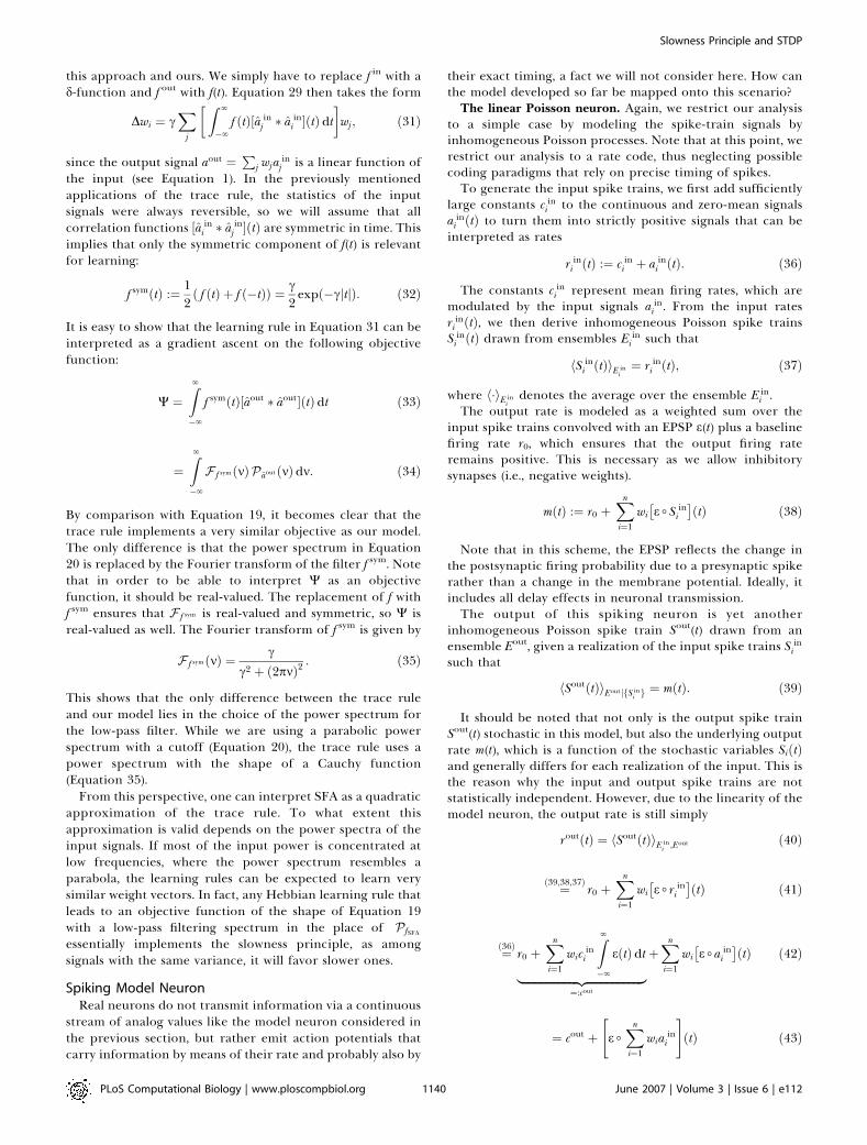
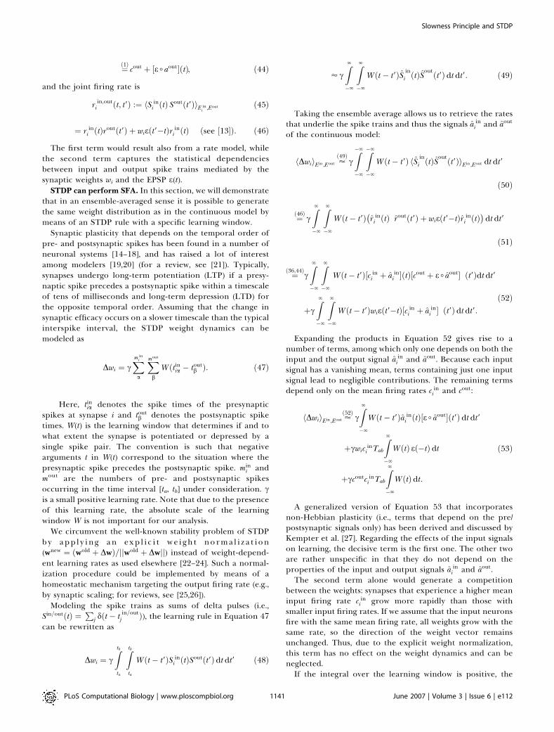
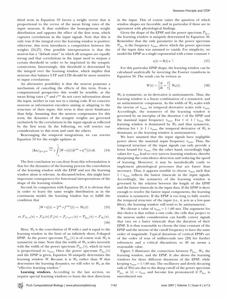
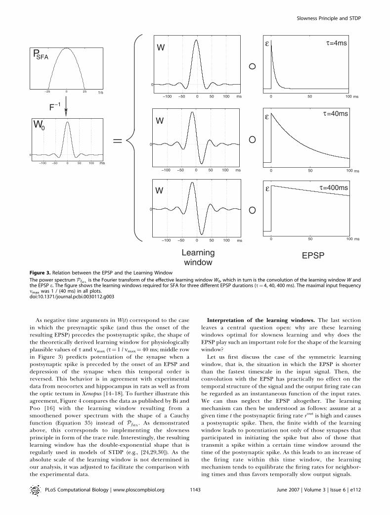
this choice is that within a rate code, the cells that project tothe neuron under consideration can hardly convey signalsthat vary on a faster timescale than the duration of theirEPSP. It is thus reasonable to choose the time constant of theEPSP and the inverse of the cutoff frequency to have the sameorder of magnitude. Typical durations of cortical EPSPs areof the order of tens of milliseconds (see [28] for furtherreferences and a critical discussion), so 40 ms seems areasonable value.Figure 3 illustrates the connection between P fSFA , W0, the

learning window, and the EPSP. It also shows the learningwindows for three different durations of the EPSP, whilekeeping mmax¼ 1 / (40 ms). The oscillatory and slowly decayingtails ofW(t) are due to the sharp cutoff of the power spectrumP fSFA at jmj ¼ mmax and become less pronounced if P fSFA issmoothened out.



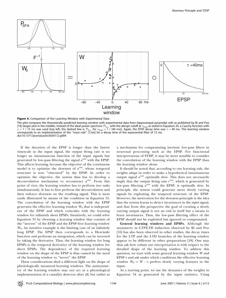
As negative time arguments in W(t) correspond to the casein which the presynaptic spike (and thus the onset of theresulting EPSP) precedes the postsynaptic spike, the shape ofthe theoretically derived learning window for physiologicallyplausible values of s and mmax (s¼1 / mmax¼ 40 ms; middle rowin Figure 3) predicts potentiation of the synapse when apostsynaptic spike is preceded by the onset of an EPSP anddepression of the synapse when this temporal order isreversed. This behavior is in agreement with experimentaldata from neocortex and hippocampus in rats as well as fromthe optic tectum in Xenopus [14–18]. To further illustrate thisagreement, Figure 4 compares the data as published by Bi andPoo [16] with the learning window resulting from asmoothened power spectrum with the shape of a Cauchyfunction (Equation 35) instead of P fSFA . As demonstratedabove, this corresponds to implementing the slownessprinciple in form of the trace rule. Interestingly, the resultinglearning window has the double-exponential shape that isregularly used in models of STDP (e.g., [24,29,30]). As theabsolute scale of the learning window is not determined inour analysis, it was adjusted to facilitate the comparison withthe experimental data.

Interpretation of the learning windows. The last sectionleaves a central question open: why are these learningwindows optimal for slowness learning and why does theEPSP play such an important role for the shape of the learningwindow?Let us first discuss the case of the symmetric learning

window, that is, the situation in which the EPSP is shorterthan the fastest timescale in the input signal. Then, theconvolution with the EPSP has practically no effect on thetemporal structure of the signal and the output firing rate canbe regarded as an instantaneous function of the input rates.We can thus neglect the EPSP altogether. The learningmechanism can then be understood as follows: assume at agiven time t the postsynaptic firing rate rout is high and causesa postsynaptic spike. Then, the finite width of the learningwindow leads to potentiation not only of those synapses thatparticipated in initiating the spike but also of those thattransmit a spike within a certain time window around thetime of the postsynaptic spike. As this leads to an increase ofthe firing rate within this time window, the learningmechanism tends to equilibrate the firing rates for neighbor-ing times and thus favors temporally slow output signals.

Figure 3. Relation between the EPSP and the Learning Window

The power spectrum P fSFA is the Fourier transform of the effective learning window W0, which in turn is the convolution of the learning window W andthe EPSP e. The figure shows the learning windows required for SFA for three different EPSP durations (s¼ 4, 40, 400 ms). The maximal input frequencymmax was 1 / (40 ms) in all plots.doi:10.1371/journal.pcbi.0030112.g003



If the duration of the EPSP is longer than the fastesttimescale in the input signal, the output firing rate is nolonger an instantaneous function of the input signals butgenerated by low-pass filtering the signal aout with the EPSP.This affects learning, because the objective of the continuousmodel is to optimize the slowness of aout, whose temporalstructure is now ‘‘obscured’’ by the EPSP. In order tooptimize the objective, the system thus has to develop adeconvolution mechanism to reconstruct aout. From thispoint of view, the learning window has to perform two taskssimultaneously. It has to first perform the deconvolution andthen enforce slowness on the resulting signal. This is mosteasily illustrated by means of the condition in Equation 55.The convolution of the learning window with the EPSPgenerates the effective learning window W0 that is independ-ent of the EPSP and which coincides with the learningwindow for infinitely short EPSPs. Intuitively, we could solveEquation 55 by choosing a learning window that consists ofthe ‘‘inverse’’ of the EPSP and the EPSP-free learning windowW0. An intuitive example is the limiting case of an infinitelylong EPSP. The EPSP then corresponds to a Heavisidefunction and performs an integration, which can be invertedby taking the derivative. Thus, the learning window for longEPSPs is the temporal derivative of the learning window forshort EPSPs. The dependence of the required learningwindow on the shape of the EPSP is thus caused by the needof the learning window to ‘‘invert’’ the EPSP.

These considerations shed a different light on the shape ofphysiologically measured learning windows. The antisymme-try of the learning window may not act as a physiologicalimplementation of a causality detector after all, but rather as

a mechanism for compensating intrinsic low-pass filters inneuronal processing such as the EPSP. For functionalinterpretations of STDP, it may be more sensible to considerthe convolution of the learning window with the EPSP thanthe learning window alone.It should be noted that, according to our learning rule, the

weights adapt in order to make a hypothetical instantaneousoutput signal aout optimally slow. This does not necessarilyimply that the output firing rate rout, which is generated bylow-pass filtering aout with the EPSP, is optimally slow. Inprinciple, the system could generate more slowly varyingsignals by exploiting the temporal structure of the EPSP.However, the motivation for the slowness principle is the ideathat the system learns to detect invariances in the input signal,and that from this perspective the goal of creating a slowlyvarying output signal is not an end in itself but a means tolearn invariances. Thus, the low-pass filtering effect of theEPSP should not be exploited but ignored or compensated.General learning windows and EPSPs. Although the

asymmetry in LTP/LTD induction observed by Bi and Poo[16] has also been observed in other studies, the decay timesfor the LTP and the LTD branches of the learning windowappear to be different in other preparations [18]. One maythus ask how robust our interpretation is with respect to thedetailed shape of the learning window. To address thisquestion, we start with some general learning window W andEPSP e and ask under which conditions the effective learningwindow W0 ¼ W 8 e prefers slowly varying features in theinput.As a starting point, we use the dynamics of the weights in

Equation 54 as generated by the input statistics. Using

Figure 4. Comparison of the Learning Window with Experimental Data

The plot compares the theoretically predicted learning window with experimental data from hippocampal pyramidal cells as published by Bi and Poo[16] (larger plot in the middle). Instead of the ideal power spectrum P fSFA with the abrupt cutoff at mmax as stated in Equation 20, a Cauchy function withc ¼ 1 / 15 ms was used (top left, the dashed line is P fSFA for mmax ¼ 1 / (40 ms)). Again, the EPSP decay time was s ¼ 40 ms. This learning windowcorresponds to an implementation of the ‘‘trace rule’’ [1,4,6] for a decay time of the exponential filter of 15 ms.doi:10.1371/journal.pcbi.0030112.g004



aout ¼P

j wja inj and defining the correlation functions

CijðtÞ ¼ ½a inj � a in

i �ðtÞ yields

hDwiiEin ;Eout ¼X

jcZ

W0ðtÞCijðtÞdt� �|fflfflfflfflfflfflfflfflfflfflfflfflfflfflfflfflffl{zfflfflfflfflfflfflfflfflfflfflfflfflfflfflfflfflffl}

¼:Aij

wj: ð59Þ

The dynamics thus follows a linear difference equation with adynamic matrix Aij whose properties are determined by thecorrelation function Cij(t) and the effective learning windowW0(t). One important question is whether the weightsapproach a stable fixed-point state or oscillate. In thiscontext, the symmetry properties of Aij and thus those of Cij

are crucial. The correlation functions obey the relation

CijðtÞ ¼ Cjið�tÞ; ð60Þ

which couples their spatial symmetry (i.e., the symmetry withrespect to the indices i and j) to their temporal symmetry. Forinstance, if the input statistics are reversible, i.e., for Cij(t) ¼Cij(�t), Cij is symmetric in the indices and so is Aij. If the inputstatistics were ‘‘perfectly irreversible,’’ i.e., Cij(t)¼� Cij(�t), Cij

and Aij would be antisymmetric. This motivates the splittingof the correlation functions Cij into a temporally symmetricand an antisymmetric component: Cij¼Cij

þþCij�with Cij

6(t)¼6Cij

6(�t). In a similar fashion, we split the effective learningwindow W0 ¼ W0

þ þ W0�. For symmetry reasons, the

dynamical matrix Aij can then be separated into twocomponents

Aij ¼ cZ

Wþ0 ðtÞC þij ðtÞdt|fflfflfflfflfflfflfflfflfflfflfflfflfflfflfflffl{zfflfflfflfflfflfflfflfflfflfflfflfflfflfflfflffl}¼:A þij

þ cZ

W �0 ðtÞC �ij ðtÞdt|fflfflfflfflfflfflfflfflfflfflfflfflfflfflfflffl{zfflfflfflfflfflfflfflfflfflfflfflfflfflfflfflffl}¼:A �ij

: ð61Þ

Because of the symmetry relation in Equation 60, Aijþ is

symmetric in i and j, while Aij� is antisymmetric. This shows

that the effective learning window W0 can be split into twofunctionally different components. The symmetric compo-nent picks up the reversible aspects of the input statisticswhile the antisymmetric component detects irreversibilities,e.g., possible causal relations within the input data. It is thisantisymmetric component of the learning window that haspreviously been interpreted as a means for sequence learningand predictive coding [19,31]. Note that the associated weightupdate

PjAij�wj is always orthogonal to the weight itself.

Thus, irreversibilities in the input data in combination withan antisymmetric learning window work against the develop-ment of a stable weight distribution, even if the inputstatistics are stationary. In particular, weight oscillations onthe timescale of learning may occur. For instance, in networkswith recurrent connections that learn according to STDP,previous studies have shown that the network tends todevelop a state of distributed synchrony [32] that resemblessynfire chains. These activity patterns display a pronouncedcausal structure, so it would be interesting to check if thesynaptic weights that emerge in such a network are stable orshow oscillations. It is likely that in this context the modelconstraints on the weights play an important role. If theweights are limited by hard boundaries as in [32], they tend tosaturate, thereby avoiding oscillatory solutions. In the case ofsofter weight constraints, e.g., in models of STDP withmultiplicative weight-dependence, oscillations may occur.

If W0 is symmetric or if the input statistics are reversible,

Cij� ¼ 0, the dynamical matrix Aij ¼ Aij

þ is symmetric. Asalready seen for the case of the continuous model neuron, thelearning dynamics can then be interpreted as a gradientascent on the objective function

W ¼ 12

Xi;j

wiA þij wj ¼12

ZW þ

0 ðmÞPaoutðmÞdm: ð62Þ

As discussed earlier, this objective function can beinterpreted as an implementation of the slowness principleif W0

þ(m) is a low-pass filter, i.e., it has a global maximum atzero frequency. This indicates that at least for reversibleinput statistics the preference of STDP for slow signals maybe rather insensitive to details of the learning window.

Discussion

Neurons in the central nervous system display a wide rangeof invariances in their response behavior, examples of whichare phase invariance in complex cells in the early visualsystem [33], head direction invariance in hippocampal placecells [34], or more complex invariances in neurons associatedwith face recognition [35]. If these invariances are learned,the associated learning rule must somehow reflect a heuristicsas to which sensory stimuli are supposed to be categorized asbeing the same. Objects in our environment are unlikely tochange completely from one moment to the next but ratherundergo typical transformations. Intuitively, responses ofneurons with invariances to these transformations shouldthus vary more slowly than others. The slowness principleuses this intuition and conjectures that neurons learn theseinvariances by favoring slowly varying output signals withoutexploiting low-pass filtering.SFA [10] is one implementation of the slowness principle in

that it minimizes the mean square of the temporal derivativeof the output signal for a given set of training data. SFA hasbeen used to model a wide range of physiologically observedproperties of complex cells in primary visual cortex [8] as wellas translation, rotation, and other invariances in the visualsystem [10]. In combination with a sparse coding objective,SFA has also been used to describe the self-organizedformation of place cells in the hippocampal formation [11].The algorithm that underlies SFA is rather technical, and it

has not yet been examined whether it is feasible to implementSFA within the limitations of neuronal circuitry. In this paperwe approach this question analytically and demonstrate thatsuch an implementation is possible in both continuous andspiking model neurons.In the first part of the paper, we show that for linear

continuous model neurons, the slowest direction in the inputsignal can be learned by means of Hebbian learning on low-pass filtered versions of the input and the output signal. Thepower spectrum of the low-pass filter required for imple-menting SFA can be derived from the learning objective andhas the shape of an upside-down parabola.The idea of using low-pass filtered signals for invariance

learning is a feature that our model has in common withseveral others [1,4,6]. By means of the continuous modelneuron, we have discussed the relation of our model to these‘‘trace rules’’ and have shown that they bear strongsimilarities.The second part of the paper discusses the modifications



that have to be made to adjust the learning rule for a Poissonneuron. We find that in an ensemble-averaged sense it ispossible to reproduce the behavior of the continuous modelneuron by means of spike-timing–dependent plasticity(STDP). Our study suggests that the outcome of STDPlearning is not governed by the learning window alone butrather by the convolution of the learning window with theEPSP, which is of relevance for functional interpretations ofSTDP.

The learning window that realizes SFA can be calculatedanalytically. Its shape is determined by the interplay of theduration of the EPSP and the maximal input frequency mmax,above which the input signals are assumed to have negligiblepower. If mmax is small, i.e., if the EPSP is sufficiently short totemporally resolve the most quickly varying components ofthe input data, the learning window is symmetric, whereas forlarge mmax or long EPSPs, it is antisymmetric. Interestingly,physiologically plausible parameters lead to a learningwindow whose shape and width is in agreement withexperimental findings. Based on this result, we propose anew functional interpretation of the STDP learning windowas an implementation of the slowness principle thatcompensates for neuronal low-pass filters such as the EPSP.

An important question in this context is on whichtimescales is this interpretation valid. It is conceivable thatfor signals that vary on a timescale of less than a hundredmilliseconds, a learning window with a width of tens ofmilliseconds can distinguish slower from faster signals. STDPcould thus be sufficient to establish invariant representationsin early sensory processing, e.g., visual receptive fields thatbecome invariant to microsaccades inducing small trans-lations. Although it is unlikely that STDP alone candistinguish between signals that vary on behavioral timescalesof hundreds of milliseconds or even seconds, this may not beproblematic, because it is probably not sensible to order allaspects of the stimuli according to how quickly they vary.Rather, one should distinguish input components that vary soquickly that they are unlikely to be behaviorally relevant fromthose that vary on behavioral timescales. From this perspec-tive, the intrinsic timescale of the learning rule should besuch that its discriminative power is best on a timescale wherethis transition occurs. It is conceivable that this transitiontimescale lies on the order of several tens of milliseconds. Thelearning of high level invariances that correspond tobehavioral timescales will probably require additional mech-anisms with corresponding intrinsic timescales, e.g., sustainedfiring in response to a stimulus [36].

For general learning windows and EPSPs, the convolutionof the learning window with the EPSP can be split into asymmetric component and an antisymmetric component.The symmetric component picks up reversible aspects of theinput statistics while the antisymmetric component detectsirreversible aspects. Previous functional interpretations ofSTDP have mostly concentrated on the antisymmetriccomponent, which has been interpreted, e.g., as a mechanismfor sequence learning or predictive coding [19,31] or forreducing recurrent connectivity in favor of feed-forwardstructures [30,32]. Other studies have neglected the phasestructure of the learning window altogether and concen-trated on its power spectrum, proposing that timing-depend-ent plasticity performs Hebbian learning on an optimalestimate of the input signals in the presence of noise [37,38].

Note that these interpretations are not necessarily contra-dictory to ours, because the slowness interpretation relies onthe symmetric component of the learning window only andthus on the reversible aspect of the input statistics. Theseconsiderations indicate that depending on the temporalstructure of the input, STDP may have different functionalroles.A different approach to unsupervised learning of invari-

ances with a biologically realistic model neuron has beentaken by Kording and Konig [39]. In their model, bursts ofbackpropagating spikes gate synaptic plasticity by providingsufficient amounts of dendritic depolarization. These burstsare assumed to be triggered by lateral connections that evokecalcium spikes in the apical dendrites of cortical pyramidalcells.Of course the model presented here is not a complete

implementation of SFA. We have only considered the centralstep of SFA, the extraction of the most slowly varyingdirection from a set of whitened input signals. To implementthe full algorithm, additional steps are necessary: a nonlinearexpansion of the input space, the whitening of the expandedinput signals, and a means of normalizing the weights. Whentraversing the dendritic arborizations of a postsynapticneuron, axons often make more than one synaptic contact.As different input channels may be subjected to differentnonlinearities in the dendritic tree (cf. [40]), the postsynapticneuron may have access to several nonlinearly transformedversions of the same presynaptic signals. Conceptually, thisresembles a nonlinear expansion of the input signals.However, it is not obvious how these signals could bewhitened within the dendrite. On the network level, however,whitening could be achieved by adaptive recurrent inhibitionbetween the neurons [41]. This mechanism may also besuitable for extracting several slow uncorrelated signals asrequired in the original formulation of SFA [10] instead ofjust one. We assumed an explicit weight normalization in thedescription of our model. However, one could also use amodified learning rule that implicitly normalizes the weightvector as long as it extracts the signal with the largestvariance. A possible biological mechanism is synaptic scaling[25], which is believed to multiplicatively rescale all synapticweights according to postsynaptic activity, similar to Oja’srule [26,42]. Thus, it appears that most of the mechanismsnecessary for an implementation of the full SFA algorithmare available, but that it is not yet clear how to combine themin a biologically plausible way.Another critical point in the analytical derivation for the

spiking model is the replacement of the temporal by theensemble average, as this allows recovery of the rates thatunderlie the Poisson processes. The validity of the analyticalresults thus requires some kind of ergodicity in the trainingdata, a condition which of course needs to be justified for thespecific input data at hand.It is still open whether the results presented here can be

reproduced with more realistic model neurons. The spikingmodel neuron used here was simplified in that it had a linearrelationship between input and output firing rate. In manyreal neurons, highly nonlinear behavior was observed.Interestingly, Hebbian learning for nonlinear rate-basedneurons has previously been associated with the detectionof higher-order moments of the input statistics [43], therebyproviding a mechanism for extracting statistically independ-



ent components of the input signal. Because for sparse inputstatistics independent component analysis is closely related tosparse coding [44], it is tempting to speculate that within arate picture, temporally nonlocal plasticity with a nonlinearinput–output relation implements a combination of sparse-ness and slowness. Learning paradigms that combine thesetwo objectives are thus an interesting field for further studies[11,45].

Another nonlinearity that we have neglected is thefrequency- and weight-dependence of STDP [16,46]. Addi-tional work will be needed to examine how these interferewith the proposed functional role of STDP. Furthermore,modeling the spiking mechanism of a neuron by aninhomogeneous Poisson process is also a severe simplificationthat ignores basic phenomena of spike generation in bio-logical neurons such as refractoriness and thresholding. It isnot clear how these characteristics would change the learningrule that leads to an implementation of the slownessprinciple. It seems to be a very difficult task to answer thesequestions analytically. Simulations will be necessary to verifythe results derived here and to analyze which changes appearand which adaptations must be made in a more realisticmodel of neural information processing.

In summary, the analytical considerations presented hereshow that (i) slowness can be equivalently achieved byminimizing the variance of the time derivative signal or bymaximizing the variance of the low-pass filtered signal, thelatter of which can be achieved by standard Hebbian learningon the low-pass filtered input and output signals; (ii) thedifference between SFA and the trace learning rule lies in the

exact shape of the effective low-pass filter—for most practicalpurposes the results are probably equivalent; (iii) for a spikingPoisson model neuron with an STDP learning rule, it is notthe learning window that governs the weight dynamics butthe convolution of the learning window with the EPSP; (iv)the STDP learning window that implements the slownessobjective is in good agreement with learning windows foundexperimentally. With these results, we have reduced the gapbetween slowness as an abstract learning principle andbiologically plausible STDP learning rules, and we offer acompletely new interpretation of the standard STDP learningwindow.

Methods

The methods employed in this paper rely on standard mathemat-ical techniques as commonly used in the theory of synaptic plasticity(see, e.g., [47]).

Acknowledgments

We thank Christian Leibold and Richard Kempter for helpfuldiscussion. We also thank the reviewers for helping to improve themanuscript.

Author contributions. LW formulated the problem. All authorscontributed to the general line of arguments. HS and CM worked outthe details of the analysis. All authors contributed to the writing ofthe paper.

Funding. This work was generously supported by the VolkswagenFoundation.

Competing interests. The authors have declared that no competinginterests exist.

References1. Foldiak P (1991) Learning invariance from transformation sequences.

Neural Comput 3: 194–200.2. Mitchison G (1991) Removing time variation with the anti-Hebbian

differential synapse. Neural Comput 3: 312–320.3. Becker S, Hinton GE (1992) A self-organizing neural network that discovers

surfaces in random-dot stereograms. Nature 355: 161–163.4. O’Reilly RC, Johnson MH (1994) Object recognition and sensitive periods:

A computational analysis of visual imprinting. Neural Comput 6: 357–389.

5. Stone JV, Bray A (1995) A learning rule for extracting spatio–temporalinvariances. Network: Comput Neural Sys 6: 429–436.

6. Wallis G, Rolls ET (1997) Invariant face and object recognition in the visualsystem. Prog Neurobiol 51: 167–194.

7. Peng HC, Sha LF, Gan Q, Wei Y (1998) Energy function for learninginvariance in multilayer perceptron. Electronics Lett 34: 292–294.

8. Berkes P, Wiskott L (2005) Slow feature analysis yields a rich repertoire ofcomplex cells. J Vis 5: 579–602.

9. Kording KP, Kayser C, Einhauser W, Konig P (2004) How are complex cellproperties adapted to the statistics of natural stimuli? J Neurophysiol 91:206–212.

10. Wiskott L, Sejnowski T (2002) Slow feature analysis: Unsupervised learningof invariances. Neural Comput 14: 715–770.

11. Franzius M, Sprekeler H, Wiskott L (2007) Unsupervised learning of placecells, head direction cells, and spatial-view cells with slow feature analysison quasi-natural videos. Cognitive Sciences EPrint Archive (CogPrints)5492. Available: http://cogprints.org/5492/. Accessed 4 June 2007.

12. Wyss R, Konig P, Verschure PFMJ (2006) A model of the ventral visualsystem based on temporal stability and local memory. PLoS Biol 4: e120.

13. Kempter R, Gerstner W, van Hemmen JL (1999) Hebbian learning andspiking neurons. Phys Rev E 59: 4498–4514.

14. Debanne D, Gahwiler BH, Thomson SM (1994) Asynchronous pre- andpostsynaptic activity induces associative long-term depression in area CA1of the rat hippocampus. Proc Natl Acad Sci U S A 91: 1148–1152.

15. Markram H, Lubke J, Frotscher M, Sakmann B (1997) Regulation ofsynaptic efficacy by coincidence of postsynaptic APs and EPSPs. Science275: 213–215.

16. Bi G-q, Poo M-m (1998) Synaptic modifications in cultured hippocampalneurons: Dependence on spike timing, synaptic strength, and postsynapticcell type. J Neurosci 18: 10464–10472.

17. Zhang LI, Tao HW, Holt CE, Harris WA, Poo M-m (1998) A critical window

for cooperation and competition among developing retinotectal synapses.Nature 395: 37–44.

18. Feldman DE (2000) Timing-based LTP and LTD at vertical input to layer II/III pyramidal cells in rat barrel cortex. Neuron 27: 45–56.

19. Abbott LF, Blum KI (1996) Functional significance of long-term potentia-tion for sequence learning and prediction. Cereb Cortex 6: 406–416.

20. Gerstner W, Kempter R, van Hemmen JL, Wagner H (1996) A neuronallearning rule for sub-millisecond temporal coding. Nature 383: 76–78.

21. Kepecs A, van Rossum MCW, Song S, Tegner J (2002) Spike-timing–dependent plasticity: Common themes and divergent vistas. Biol Cybern 87:446–458.

22. Kistler WM, van Hemmen JL (2000) Modeling synaptic plasticity inconjunction with the timing of pre- and postsynaptic action potentials.Neural Comput 12: 385.

23. Rubin J, Lee DD, Sompolinsky H (2001) Equilibrium properties oftemporally asymmetric Hebbian learning. Phys Rev Lett 86: 364–367.

24. Gutig R, Aharonov S, Rotter S, Sompolinsky H (2003) Learning inputcorrelations through nonlinear temporally asymmetric Hebbian plasticity.J Neurosci 23: 3697–3714.

25. Turrigiano GG, Nelson SB (2000) Hebb and homeostasis in neuronalplasticity. Curr Opin Neurobiol 10: 358–364.

26. Abbott LF, Nelson SB (2000) Synaptic plasticity: Taming the beast. NatNeurosci 3: 1178–1183.

27. Kempter R, Gerstner W, van Hemmen JL (2001) Intrinsic stabilization ofoutput rates by spike-based Hebbian learning. Neural Comput 13: 2709–2741.

28. Koch C, Rapp M, Segev I (1996) A brief history of time (constants). CerebCortex 6: 92–101.

29. van Rossum MCW, Bi G-q, Turrigiano GG (2000) Stable Hebbian learningfrom spike-timing–dependent plasticity. J Neurosci 20: 8812–8821.

30. Song S, Abbott LF (2001) Cortical mapping and development throughspike-timing–dependent plasticity. Neuron 32: 339–350.

31. Rao RPN, Sejnowski TJ (2001) Spike-timing–dependent Hebbian plasticityas temporal difference learning. Neural Comput 13: 2221–2238.

32. Horn D, Levy N, Meilijson I, Ruppin E (2000) Distributed synchrony ofspiking neurons in a Hebbian cell assembly. In: Muller K-R, editor. AdvNeural Info Process Syst (NIPS) 12. Cambridge (Massachusetts): MIT Press.

33. Hubel D, Wiesel T (1968) Receptive fields and functional architecture ofmonkey striate cortex. J Physiol (Lond) 195: 215–243.

34. Muller R, Bostock E, Taube JS, Kubie JL (1994) On the directional firingproperties of hippocampal place cells. J Neurosci 14: 7235–7251.



35. Quiroga RQ, Reddy L, Kreiman G, Koch C, Fried I (2005) Invariant visualrepresentation by single neurons in the human brain. Nature 435: 1102–1107.

36. Drew PJ, Abbott LF (2006) Extending the effects of spike-timing–depend-ent plasticity to behavioral timescales. Proc Natl Acad Sci U S A 103: 8876–8881.

37. Wallis G, Baddeley R (1997) Optimal, unsupervised learning in invariantobject recognition. Neural Comput 9: 883–894.

38. Dayan P, Hausser M, London M (2004) Plasticity kernels and temporalstatistics. In: Scholkopf B, editor. Adv Neural Info Process Syst (NIPS) 16.Cambridge (Massachusetts): MIT Press.

39. Kording KP, Konig P (2001) Neurons with two sites of synaptic integrationlearn invariant representations. Neural Comput 13: 2823–2849.

40. London M, Hausser M (2005) Dendritic computation. Ann Rev Neurosci 28:503–532.

41. Barlow H, Foldiak P (1989) Adaptation and decorrelation in the cortex. In:

Durbin R, Miall C, Mitchison G. Computing neuron. New York: Addison-Wesley. 43 p.

42. Oja E (1982) A simplified neuron as a principal component analyzer. J MathBiol 15: 267–273.

43. Oja E, Karhunen J (1995) Signal separation by nonlinear Hebbian learning.Computational intelligence: A dynamic system perspective: 83–97.

44. Olshausen BA, Field DJ (1997) Sparse coding with an overcomplete basisset: A strategy employed by V1? Vision Res 37: 3311–3325.

45. Blaschke T, Zito T, Wiskott L (2007) Independent slow feature analysis andnonlinear blind source separation. Neural Comput 19: 994–1021.

46. Sjostrom PJ, Turrigiano GG, Nelson SB (2001) Rate, timing, andcooperativity jointly determine cortical synaptic plasticity. Neuron 32:1149–1164.

47. Gerstner W, Kistler WM (2002) Spiking model neurons. CambridgeUniversity Press.



slowness: an objective for spike-timing–dependent …sprekeler/data/paper/sprekeler... · one...

Documents