slide 1 hierarchical multiple regression. slide 2 differences between standard and hierarchical...
TRANSCRIPT
Slide 1
Hierarchical Multiple Regression
Slide 2
Differences between standard and hierarchical multiple regression
Standard multiple regression is used to evaluate the relationship between a set of independent variables and a dependent variable.
Hierarchical regression is used to evaluate the relationship between a set of independent variables (predictors) and the dependent variable, controlling for or taking into account the impact of a different set of independent variables (control variables) on the dependent variable.
For example, a research hypothesis might state that there are differences in the average salary between male employees and female employees, even after we take into account differences in education levels and prior work experience.
In hierarchical regression, the independent variables are entered into the analysis in a sequence of blocks, or groups that may contain one or more variables. In the example above, education and work experience would be entered in the first block and sex would be entered in the second block.
Generally, our interest is in R² change, i.e. the increase when the predictors variables are added to the analysis rather than the overall R² for the model that includes both controls and predictors.
Moreover, the interpretation of individual relationships may focus on the relationship between the predictors and the dependent variables, and ignore the significance and interpretation of control variables. However, in our problems, we will interpret both controls and predictors.
Slide 3
Differences in statistical results
SPSS shows the statistical results (Model Summary, ANOVA, Coefficients, etc.) as each block of variables is entered into the analysis.
In addition (if requested), SPSS prints and tests the key statistic used in evaluating the hierarchical hypothesis: change in R² for each additional block of variables.
The null hypothesis for the addition of each block of variables to the analysis is that the change in R² (contribution to the explanation of the variance in the dependent variable) is zero.
If the null hypothesis is rejected, then our interpretation indicates that the variables in block 2 had a relationship to the dependent variable, after controlling for the relationship of the block 1 variables to the dependent variable, i.e. the variables in block 2 explain something about the dependent variables that was not explained in block 1.
The key statistic in hierarchical regression is R² change (the increase in R² when the predictors variables are added to the model that included only the control variables). If R² change is significant, the R² for the overall model that includes both controls and predictors will usually be significant as well since R² change is part of overall R².
Slide 4
Variations in hierarchical regression
A hierarchical regression can have as many blocks as there are independent variables, i.e. the analyst can specify a hypothesis that specifies an exact order of entry for variables.
A more common hierarchical regression specifies two blocks of variables: a set of control variables entered in the first block and a set of predictor variables entered in the second block.
Control variables are often demographics which are thought to make a difference in scores on the dependent variable. Predictors are the variables in whose effect our research question is really interested, but whose effect we want to separate out from the control variables.
Hierarchical regression specifies the order in which the variables are added to the regression analysis. However, once the regression analysis includes all of the independent variable, the variables will have the same coefficients and significance independent of whether the variables were entered simultaneously or sequentially.
Slide 5
Confusion in Terminology over the Meaning of the Designation of a Control Variable
Control variables are entered in the first block in a hierarchical regression, and we describe this as “controlling for the effect of some variables…” Sometimes, we mistakenly interpret this to imply that the shared effects between a variable and the control variables is removed from the explanation of the dependent variable credited to the predictor.
In fact, the coefficient for each variable is computed to control for all other variables in the analysis, whether the variable is designated as a control or a predictor variable, and regardless of when it was entered into the equation.
In a general sense, each variable in a regression analysis is credited only with what it uniquely explains, and the shared variance with all other variables is removed.
Slide 6
Research Questions for which Hierarchical Regression is Useful
Previous research has found that variables a, b, and c have statistically significant relationships to the dependent variable z, both collectively and individually. You believe that variables d and e should also be included and, in fact, would substantially increase the proportion of variability in z that we can explain. You treat a, b, and c as controls and d and e as predictors in a hierarchical regression.
You have found that variables a and b account for a substantial proportion of the differences in the dependent variable z. In presenting your findings, someone asserts that while a and b may have a relationship to z, differences in z are better understood with the relationship that variables d and e have with z. You treat d and e as controls to show that predictors a and b have a significant relationship to z that is not explicable by d and e.
You find that there are significant differences in the demographic characteristics (a, b, and c) of groups of subjects in your control and treatment groups (d). To isolate the relationship between group membership (d) and the treatment effect (z), you do a hierarchical regression with a, b, and c as controls and d as the predictor.
Slide 7
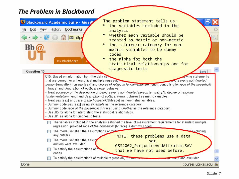
The Problem in Blackboard
The problem statement tells us: the variables included in the analysis whether each variable should be
treated as metric or non-metric the reference category for non-metric
variables to be dummy coded the alpha for both the statistical
relationships and for diagnostic tests
NOTE: these problems use a data set, GSS2002_PrejudiceAndAltruism.SAV
that we have not used before.
Slide 8
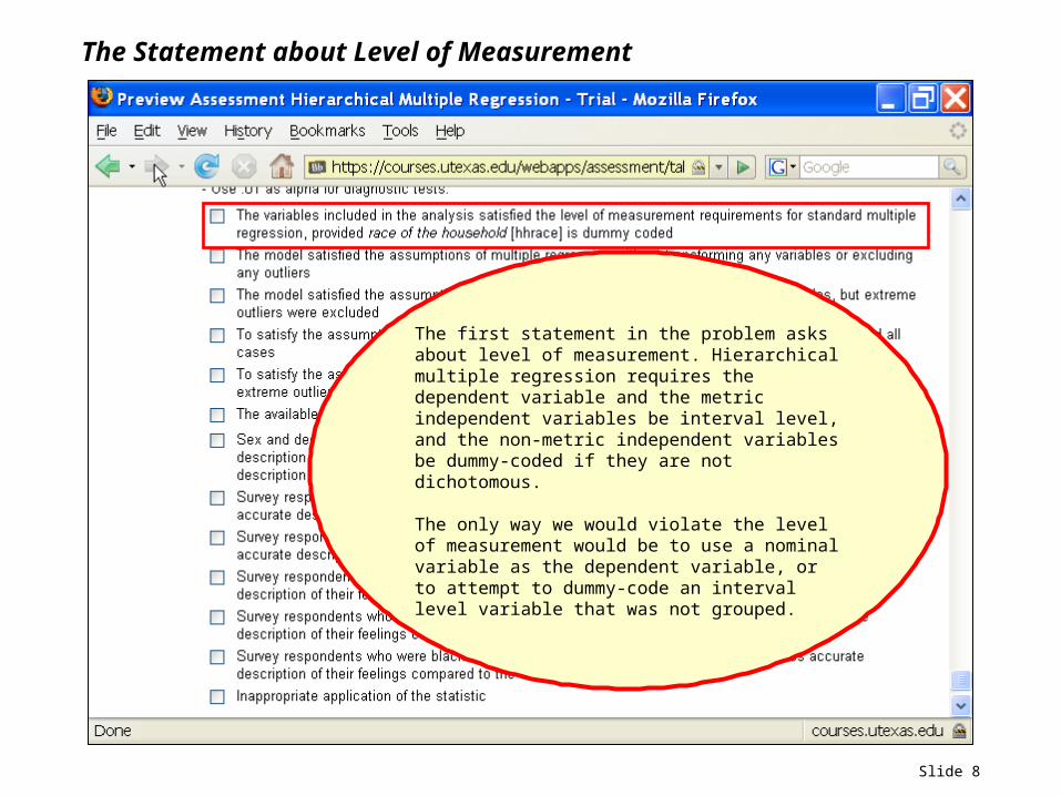
The Statement about Level of Measurement
The first statement in the problem asks about level of measurement. Hierarchical multiple regression requires the dependent variable and the metric independent variables be interval level, and the non-metric independent variables be dummy-coded if they are not dichotomous.
The only way we would violate the level of measurement would be to use a nominal variable as the dependent variable, or to attempt to dummy-code an interval level variable that was not grouped.
Slide 9
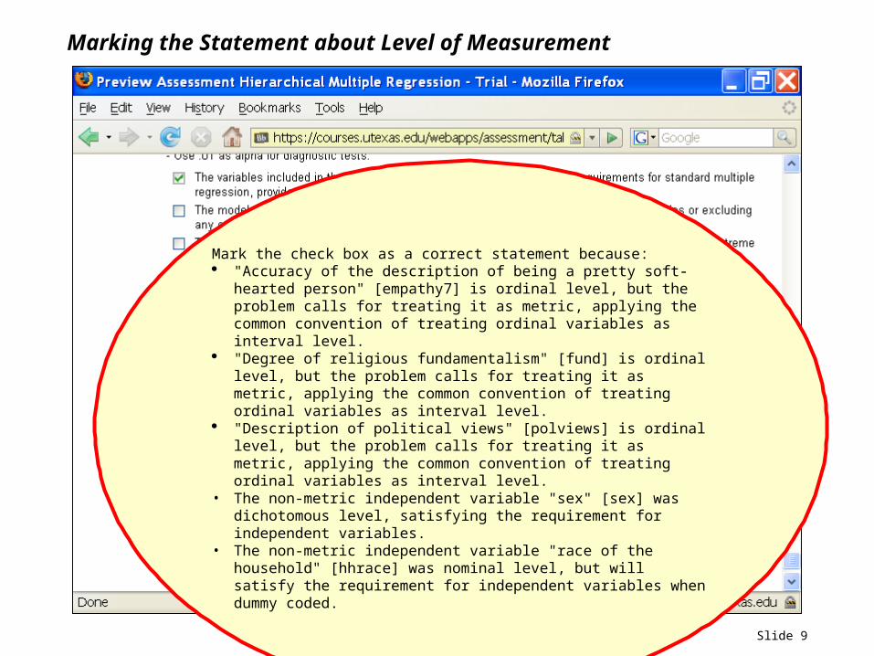
Marking the Statement about Level of Measurement
Mark the check box as a correct statement because: "Accuracy of the description of being a pretty soft-hearted
person" [empathy7] is ordinal level, but the problem calls for treating it as metric, applying the common convention of treating ordinal variables as interval level.
"Degree of religious fundamentalism" [fund] is ordinal level, but the problem calls for treating it as metric, applying the common convention of treating ordinal variables as interval level.
"Description of political views" [polviews] is ordinal level, but the problem calls for treating it as metric, applying the common convention of treating ordinal variables as interval level.
• The non-metric independent variable "sex" [sex] was dichotomous level, satisfying the requirement for independent variables.
• The non-metric independent variable "race of the household" [hhrace] was nominal level, but will satisfy the requirement for independent variables when dummy coded.
Slide 10
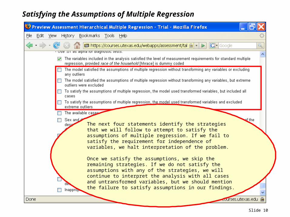
Satisfying the Assumptions of Multiple Regression
The next four statements identify the strategies that we will follow to attempt to satisfy the assumptions of multiple regression. If we fail to satisfy the requirement for independence of variables, we halt interpretation of the problem.
Once we satisfy the assumptions, we skip the remaining strategies. If we do not satisfy the assumptions with any of the strategies, we will continue to interpret the analysis with all cases and untransformed variables, but we should mention the failure to satisfy assumptions in our findings.

Slide 11
Using the Script to Evaluate Assumptions
We will use the new script to evaluate regression assumptions for analyses that include metric and non-metric variables.
Assuming that you have downloaded the script from the course web site to My Documents, select the Run Script command from the Utilities menu.
Slide 12
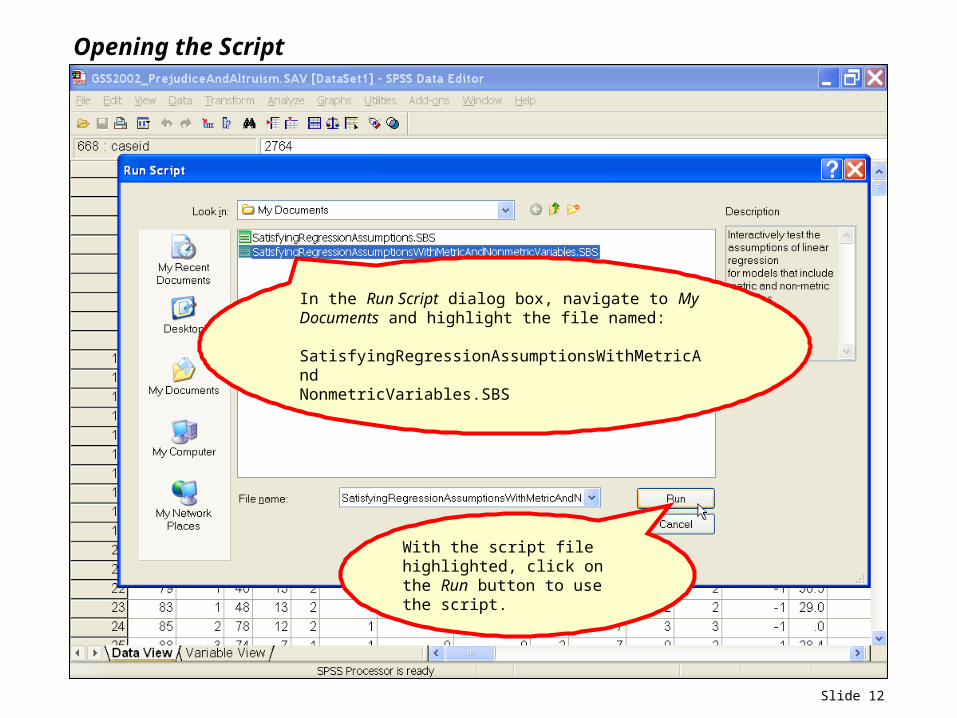
Opening the Script
In the Run Script dialog box, navigate to My Documents and highlight the file named:
SatisfyingRegressionAssumptionsWithMetricAndNonmetricVariables.SBS
With the script file highlighted, click on the Run button to use the script.
Slide 13
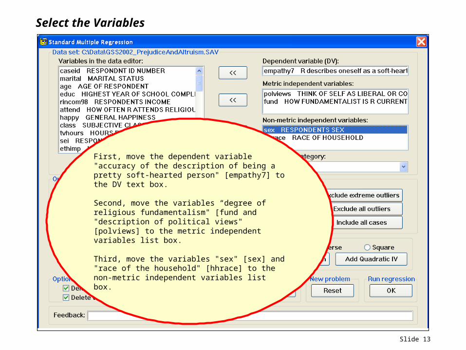
Select the Variables
First, move the dependent variable "accuracy of the description of being a pretty soft-hearted person" [empathy7] to the DV text box.
Second, move the variables “degree of religious fundamentalism" [fund and "description of political views" [polviews] to the metric independent variables list box.
Third, move the variables "sex" [sex] and "race of the household" [hhrace] to the non-metric independent variables list box.
Slide 14
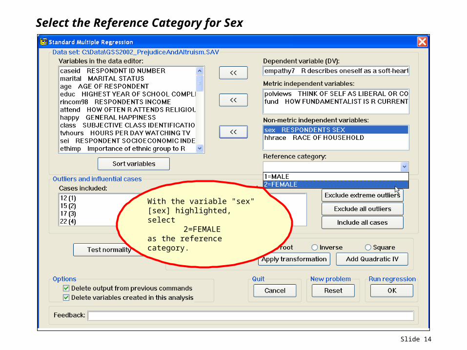
Select the Reference Category for Sex
With the variable "sex" [sex] highlighted, select
2=FEMALE as the reference category.
Slide 15
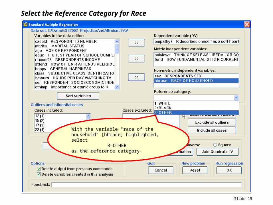
Select the Reference Category for Race
With the variable "race of the household" [hhrace] highlighted, select
3=OTHER as the reference category.
Slide 16
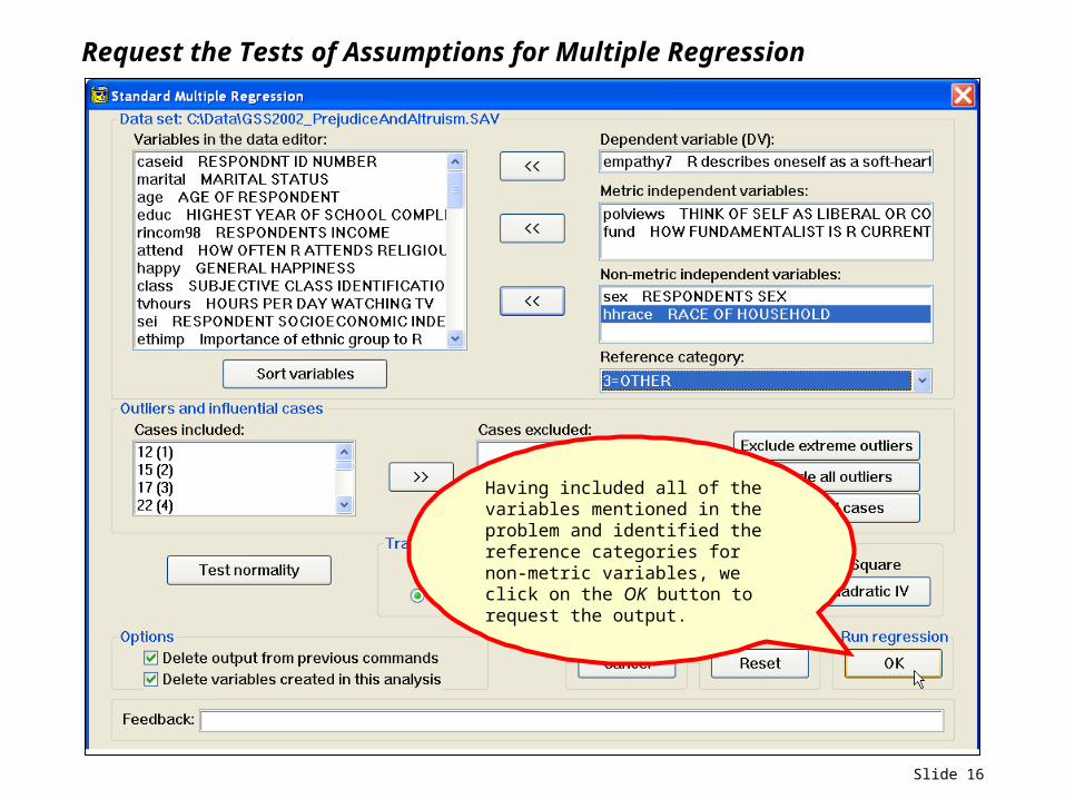
Request the Tests of Assumptions for Multiple Regression
Having included all of the variables mentioned in the problem and identified the reference categories for non-metric variables, we click on the OK button to request the output.
Slide 17
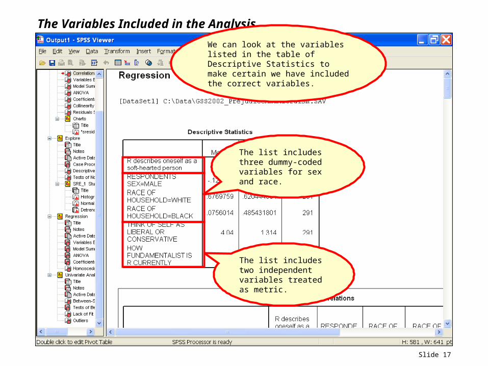
The Variables Included in the Analysis
We can look at the variables listed in the table of Descriptive Statistics to make certain we have included the correct variables.
The list includes three dummy-coded variables for sex and race.
The list includes two independent variables treated as metric.
Slide 18
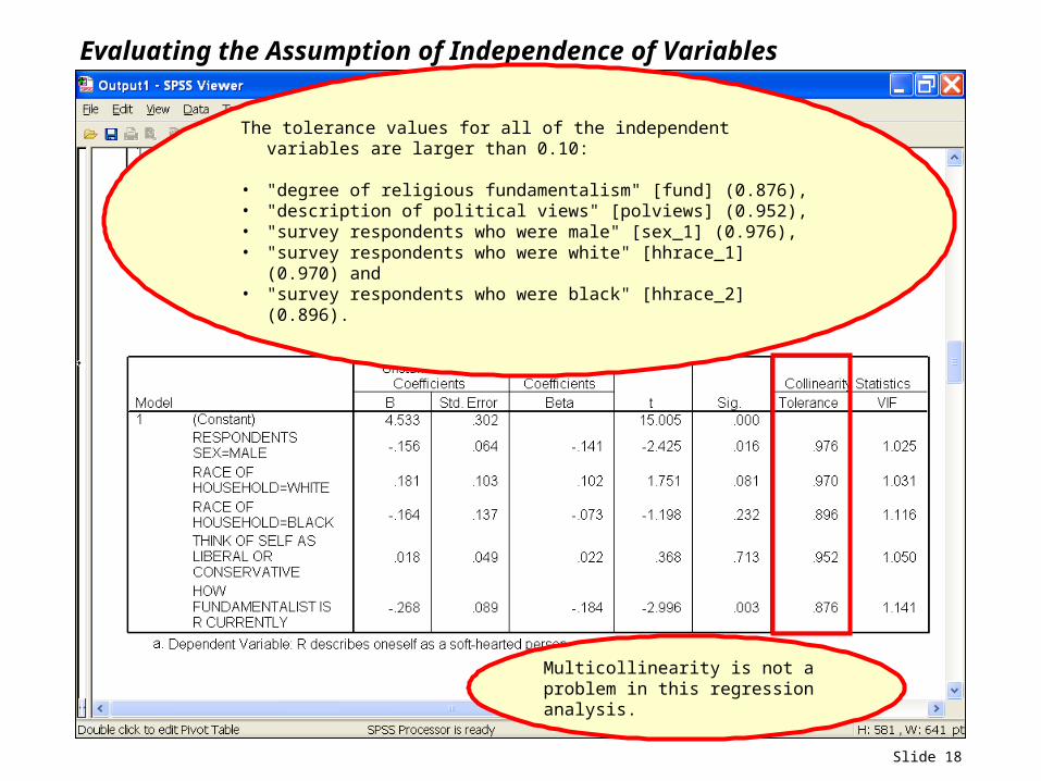
Evaluating the Assumption of Independence of Variables
The tolerance values for all of the independent variables are larger than 0.10:
• "degree of religious fundamentalism" [fund] (0.876), • "description of political views" [polviews] (0.952),• "survey respondents who were male" [sex_1] (0.976), • "survey respondents who were white" [hhrace_1] (0.970) and • "survey respondents who were black" [hhrace_2] (0.896).
Multicollinearity is not a problem in this regression analysis.
Slide 19
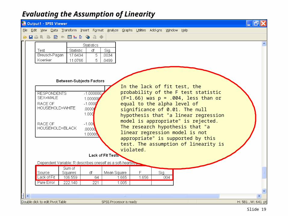
Evaluating the Assumption of Linearity
In the lack of fit test, the probability of the F test statistic (F=1.66) was p = .004, less than or equal to the alpha level of significance of 0.01. The null hypothesis that "a linear regression model is appropriate" is rejected. The research hypothesis that "a linear regression model is not appropriate" is supported by this test. The assumption of linearity is violated.
Slide 20
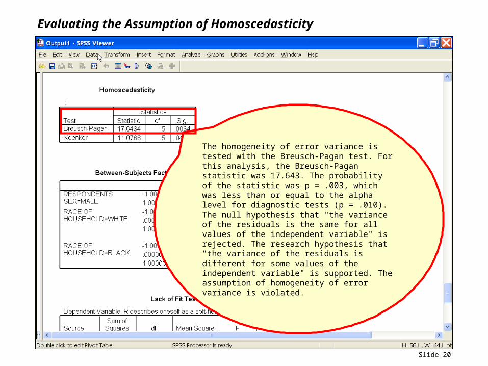
Evaluating the Assumption of Homoscedasticity
The homogeneity of error variance is tested with the Breusch-Pagan test. For this analysis, the Breusch-Pagan statistic was 17.643. The probability of the statistic was p = .003, which was less than or equal to the alpha level for diagnostic tests (p = .010). The null hypothesis that "the variance of the residuals is the same for all values of the independent variable" is rejected. The research hypothesis that "the variance of the residuals is different for some values of the independent variable" is supported. The assumption of homogeneity of error variance is violated.
Slide 21
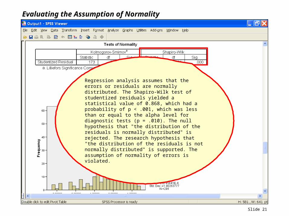
Evaluating the Assumption of Normality
Regression analysis assumes that the errors or residuals are normally distributed. The Shapiro-Wilk test of studentized residuals yielded a statistical value of 0.868, which had a probability of p < .001, which was less than or equal to the alpha level for diagnostic tests (p = .010). The null hypothesis that "the distribution of the residuals is normally distributed" is rejected. The research hypothesis that "the distribution of the residuals is not normally distributed" is supported. The assumption of normality of errors is violated.
Slide 22
Evaluating the Assumption of Independence of Errors
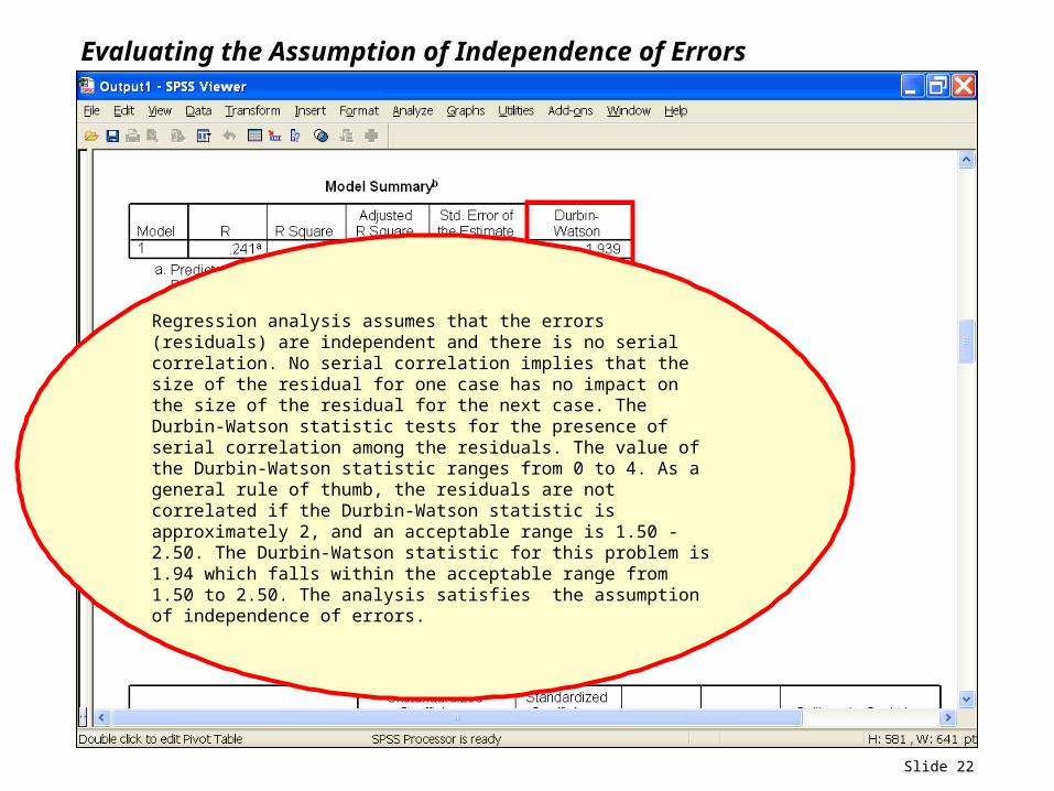
Regression analysis assumes that the errors (residuals) are independent and there is no serial correlation. No serial correlation implies that the size of the residual for one case has no impact on the size of the residual for the next case. The Durbin-Watson statistic tests for the presence of serial correlation among the residuals. The value of the Durbin-Watson statistic ranges from 0 to 4. As a general rule of thumb, the residuals are not correlated if the Durbin-Watson statistic is approximately 2, and an acceptable range is 1.50 - 2.50. The Durbin-Watson statistic for this problem is 1.94 which falls within the acceptable range from 1.50 to 2.50. The analysis satisfies the assumption of independence of errors.
Slide 23
Excluding Extreme Outliers to Try to Achieve Normality
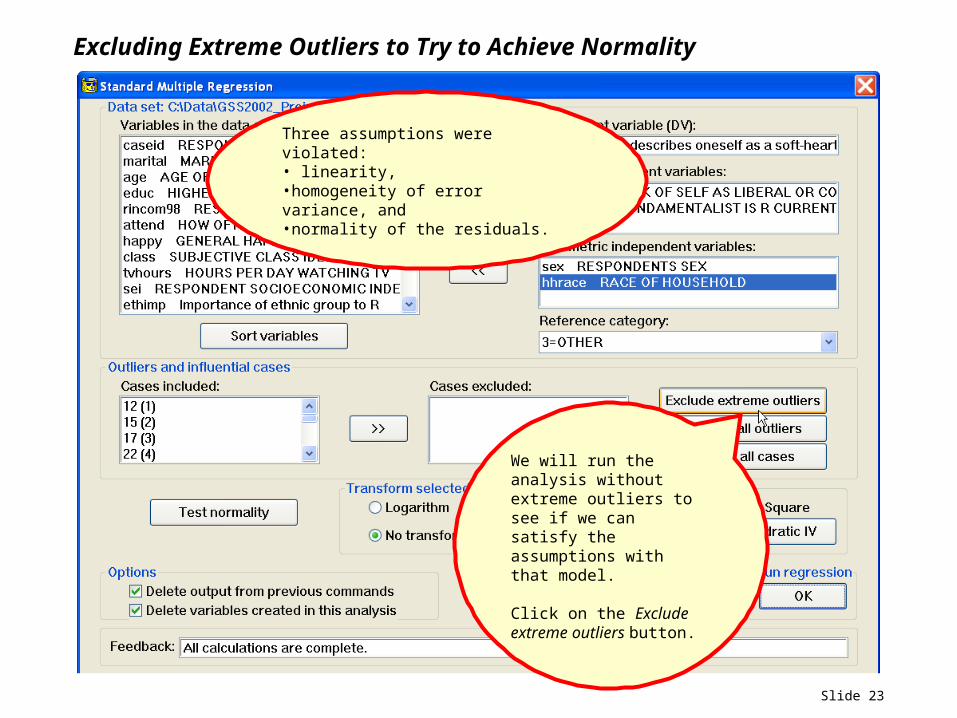
Three assumptions were violated:• linearity, •homogeneity of error variance, and •normality of the residuals.
We will run the analysis without extreme outliers to see if we can satisfy the assumptions with that model.
Click on the Exclude extreme outliers button.
Slide 24
Feedback on Extreme Outliers
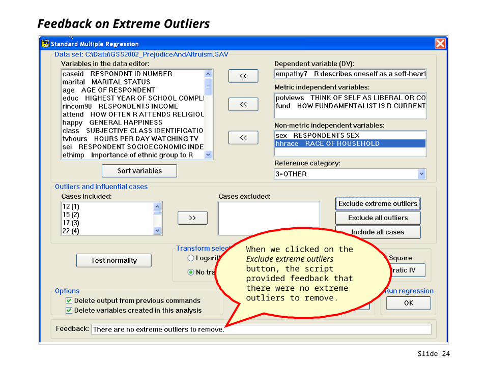
When we clicked on the Exclude extreme outliers button, the script provided feedback that there were no extreme outliers to remove.
Slide 25
Outliers and Extreme Outliers in SPSS Output
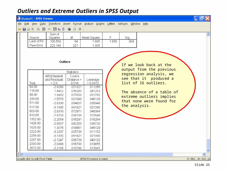
If we look back at the output from the previous regression analysis, we see that it produced a list of 16 outliers.
The absence of a table of extreme outliers implies that none were found for the analysis.
Slide 26
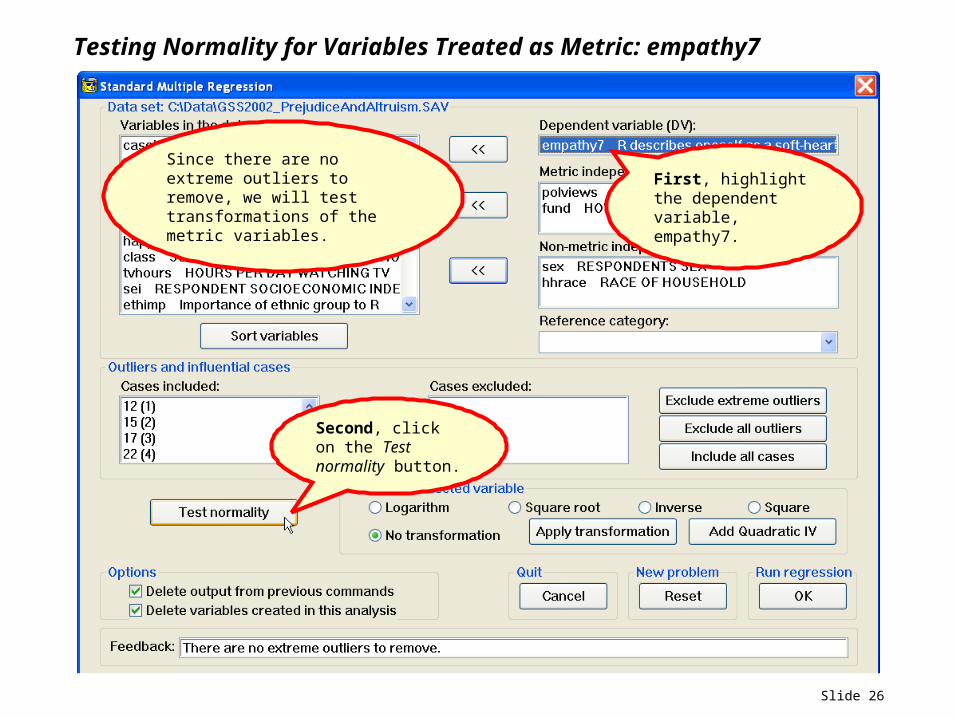
Testing Normality for Variables Treated as Metric: empathy7
Since there are no extreme outliers to remove, we will test transformations of the metric variables.
First, highlight the dependent variable, empathy7.
Second, click on the Test normality button.
Slide 27
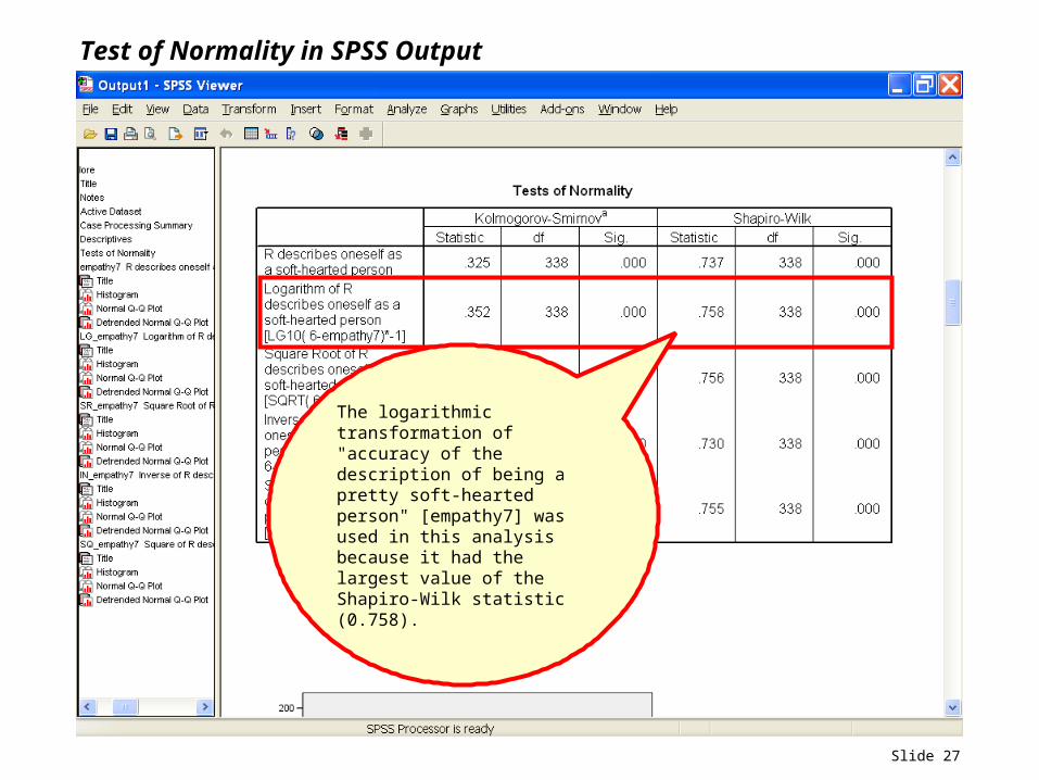
Test of Normality in SPSS Output
The logarithmic transformation of "accuracy of the description of being a pretty soft-hearted person" [empathy7] was used in this analysis because it had the largest value of the Shapiro-Wilk statistic (0.758).
Slide 28
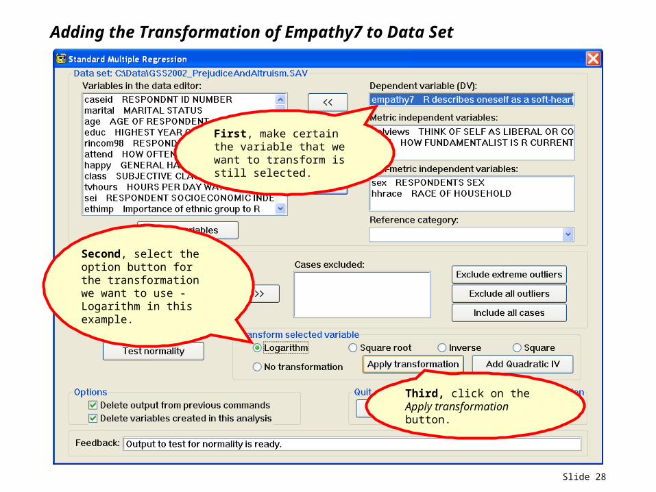
Adding the Transformation of Empathy7 to Data Set
First, make certain the variable that we want to transform is still selected.
Second, select the option button for the transformation we want to use - Logarithm in this example.
Third, click on the Apply transformation button.
Slide 29
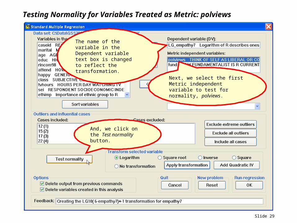
Testing Normality for Variables Treated as Metric: polviews
The name of the variable in the Dependent variable text box is changed to reflect the transformation.
Next, we select the first Metric independent variable to test for normality, polviews.
And, we click on the Test normality button.

Slide 30
Test of Normality in SPSS Output
No transformation of "description of political views" [polviews] was used in this analysis. None of the transformations had a value of the Shapiro-Wilk statistic that was at least 0.01 larger than the value for description of political views (0.924).
Slide 31
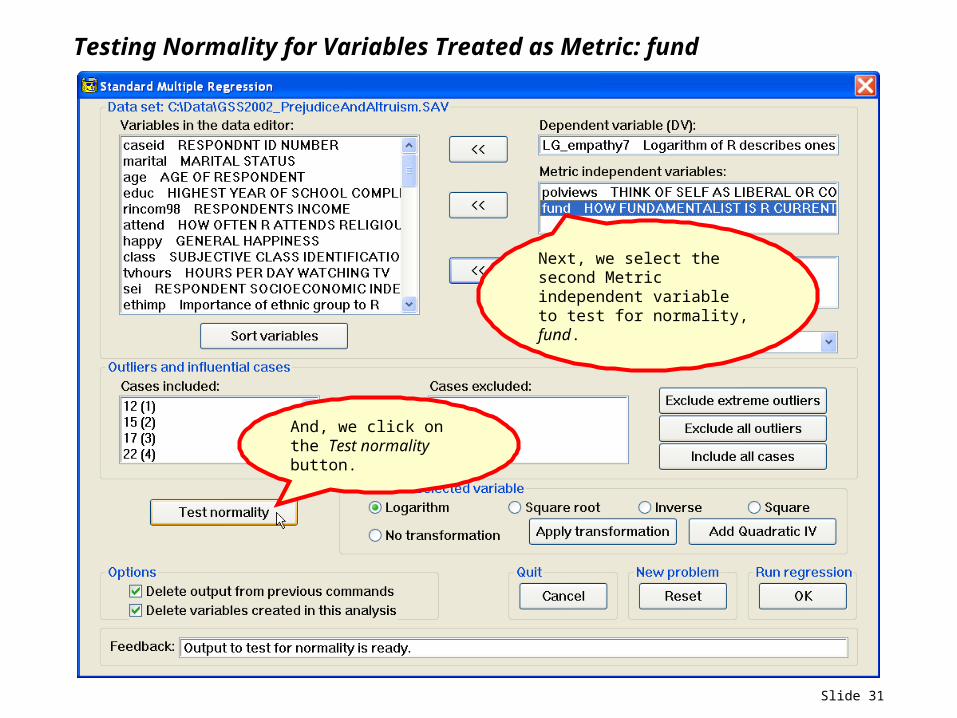
Testing Normality for Variables Treated as Metric: fund
Next, we select the second Metric independent variable to test for normality, fund.
And, we click on the Test normality button.
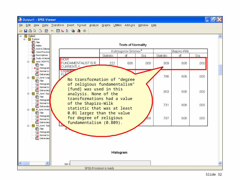
Slide 32
No transformation of "degree of religious fundamentalism" [fund] was used in this analysis. None of the transformations had a value of the Shapiro-Wilk statistic that was at least 0.01 larger than the value for degree of religious fundamentalism (0.809).
Slide 33
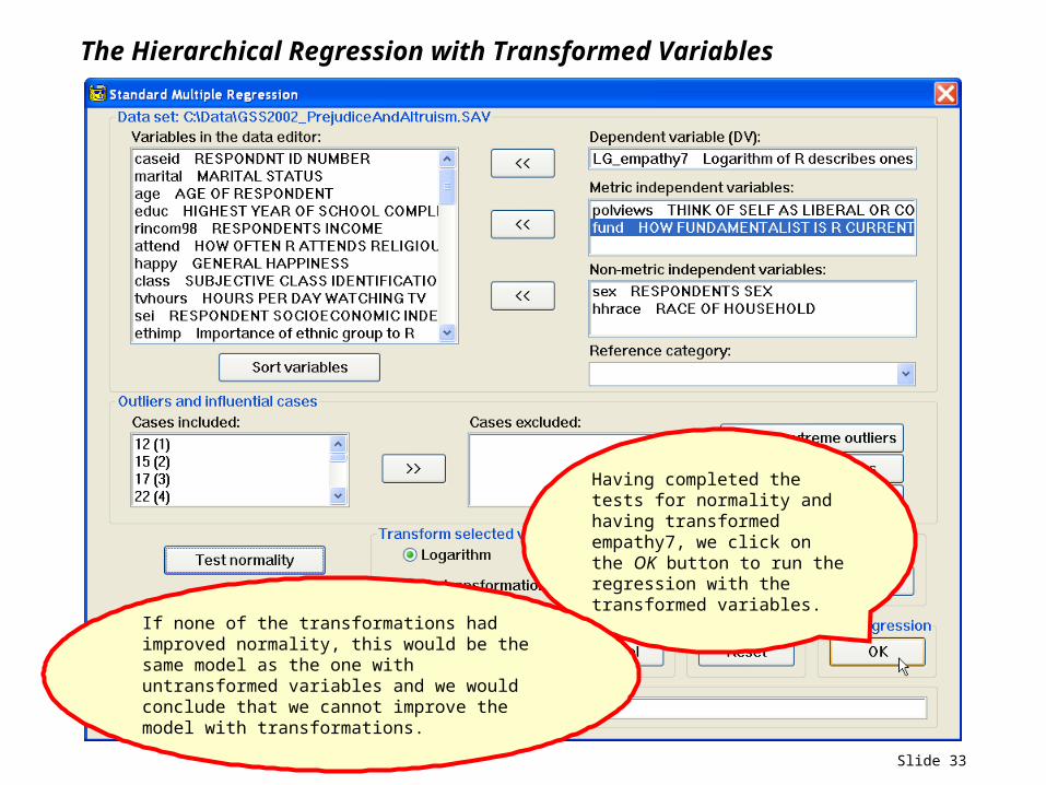
The Hierarchical Regression with Transformed Variables
Having completed the tests for normality and having transformed empathy7, we click on the OK button to run the regression with the transformed variables.
If none of the transformations had improved normality, this would be the same model as the one with untransformed variables and we would conclude that we cannot improve the model with transformations.
Slide 34
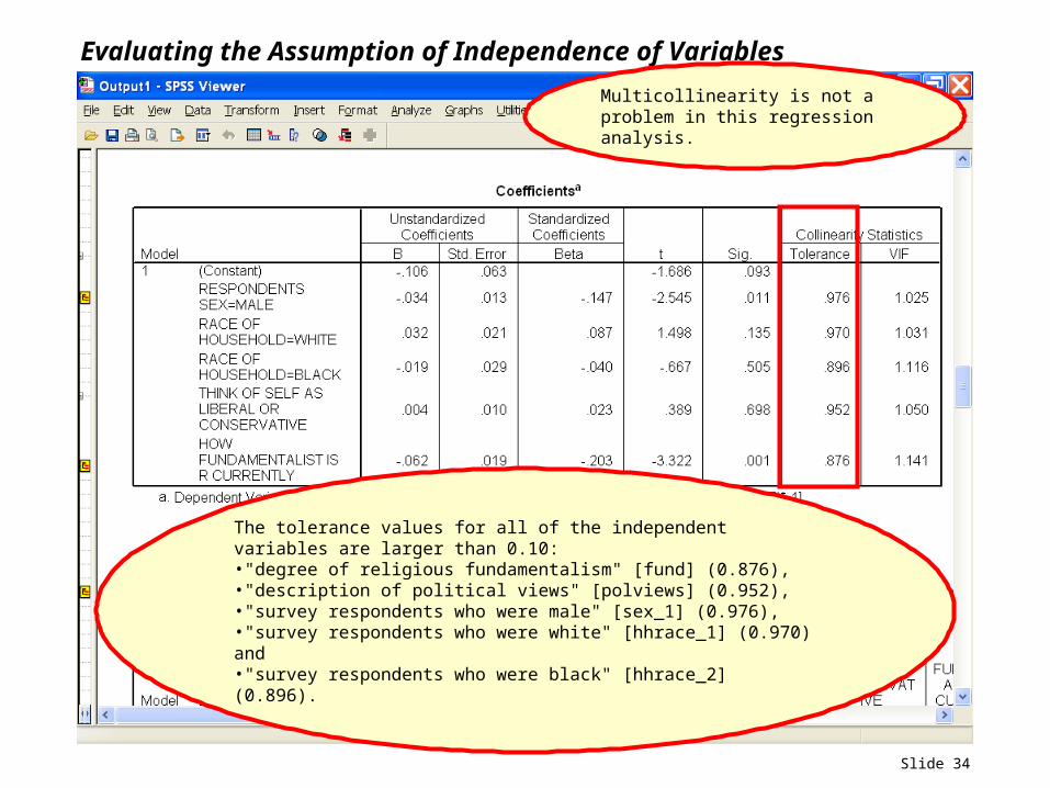
Evaluating the Assumption of Independence of Variables
The tolerance values for all of the independent variables are larger than 0.10: •"degree of religious fundamentalism" [fund] (0.876), •"description of political views" [polviews] (0.952), •"survey respondents who were male" [sex_1] (0.976), •"survey respondents who were white" [hhrace_1] (0.970) and •"survey respondents who were black" [hhrace_2] (0.896).
Multicollinearity is not a problem in this regression analysis.
Slide 35
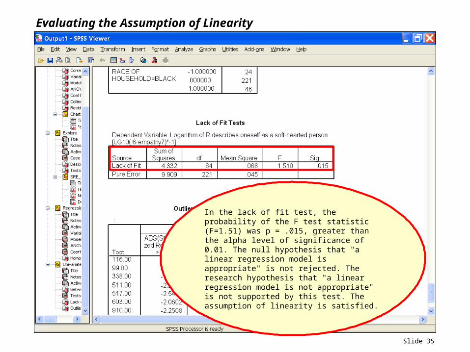
Evaluating the Assumption of Linearity
In the lack of fit test, the probability of the F test statistic (F=1.51) was p = .015, greater than the alpha level of significance of 0.01. The null hypothesis that "a linear regression model is appropriate" is not rejected. The research hypothesis that "a linear regression model is not appropriate" is not supported by this test. The assumption of linearity is satisfied.
Slide 36
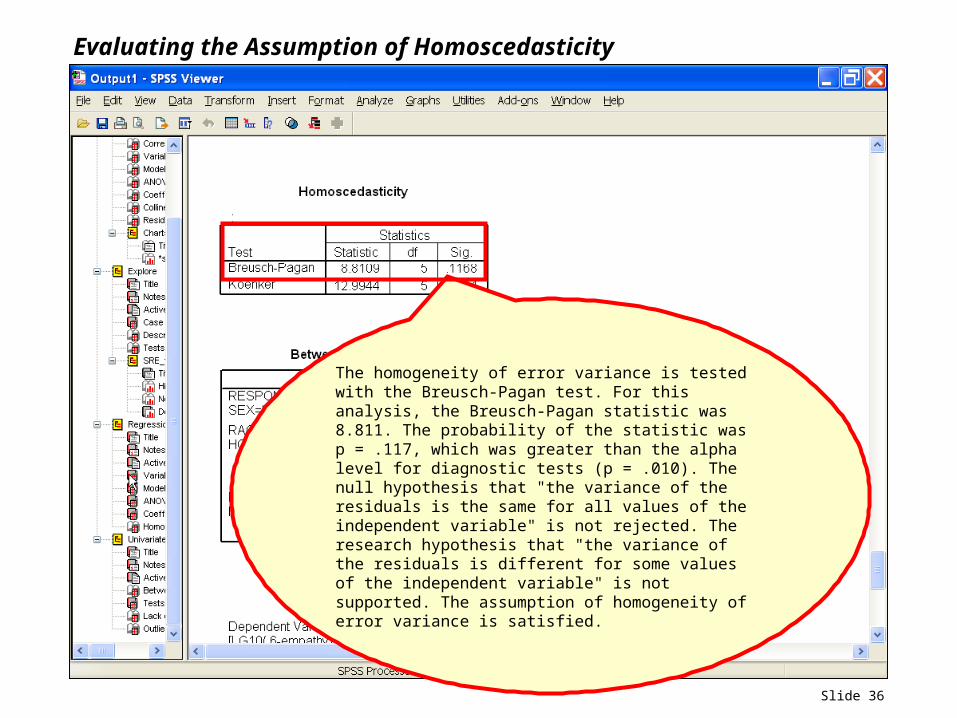
Evaluating the Assumption of Homoscedasticity
The homogeneity of error variance is tested with the Breusch-Pagan test. For this analysis, the Breusch-Pagan statistic was 8.811. The probability of the statistic was p = .117, which was greater than the alpha level for diagnostic tests (p = .010). The null hypothesis that "the variance of the residuals is the same for all values of the independent variable" is not rejected. The research hypothesis that "the variance of the residuals is different for some values of the independent variable" is not supported. The assumption of homogeneity of error variance is satisfied.
Slide 37
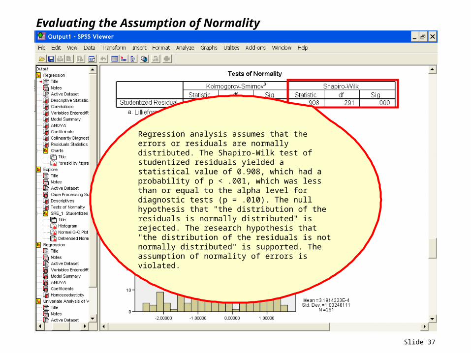
Evaluating the Assumption of Normality
Regression analysis assumes that the errors or residuals are normally distributed. The Shapiro-Wilk test of studentized residuals yielded a statistical value of 0.908, which had a probability of p < .001, which was less than or equal to the alpha level for diagnostic tests (p = .010). The null hypothesis that "the distribution of the residuals is normally distributed" is rejected. The research hypothesis that "the distribution of the residuals is not normally distributed" is supported. The assumption of normality of errors is violated.
Slide 38
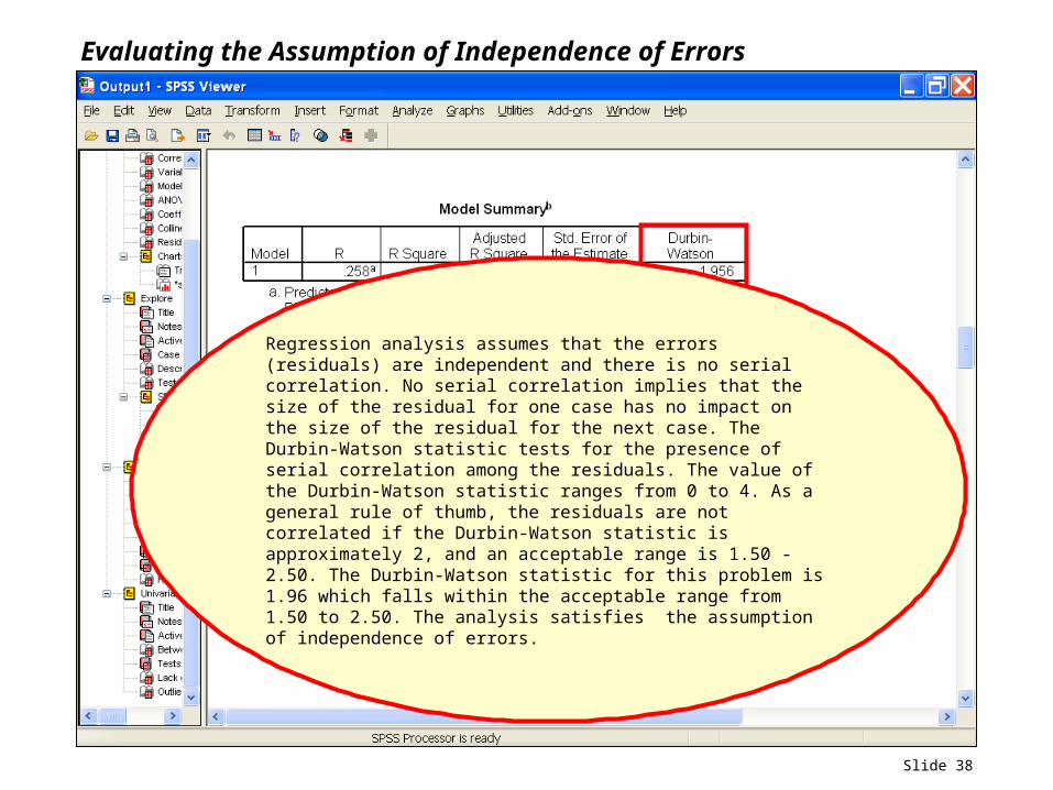
Evaluating the Assumption of Independence of Errors
Regression analysis assumes that the errors (residuals) are independent and there is no serial correlation. No serial correlation implies that the size of the residual for one case has no impact on the size of the residual for the next case. The Durbin-Watson statistic tests for the presence of serial correlation among the residuals. The value of the Durbin-Watson statistic ranges from 0 to 4. As a general rule of thumb, the residuals are not correlated if the Durbin-Watson statistic is approximately 2, and an acceptable range is 1.50 - 2.50. The Durbin-Watson statistic for this problem is 1.96 which falls within the acceptable range from 1.50 to 2.50. The analysis satisfies the assumption of independence of errors.
Slide 39
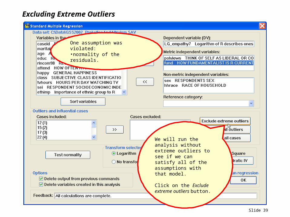
Excluding Extreme Outliers
One assumption was violated:•normality of the residuals.
We will run the analysis without extreme outliers to see if we can satisfy all of the assumptions with that model.
Click on the Exclude extreme outliers button.
Slide 40
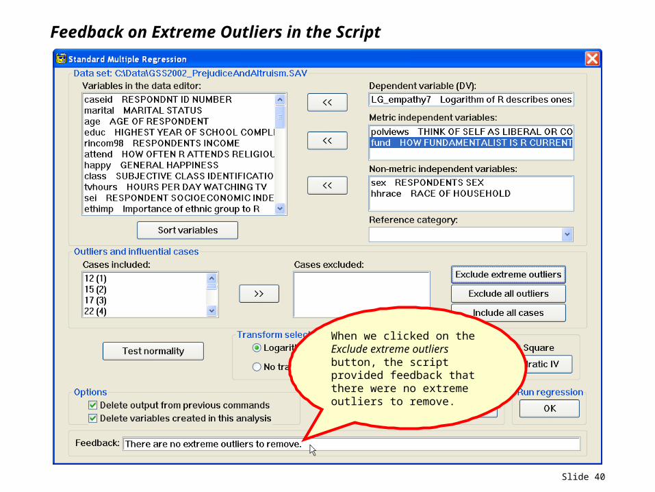
Feedback on Extreme Outliers in the Script
When we clicked on the Exclude extreme outliers button, the script provided feedback that there were no extreme outliers to remove.
Slide 41
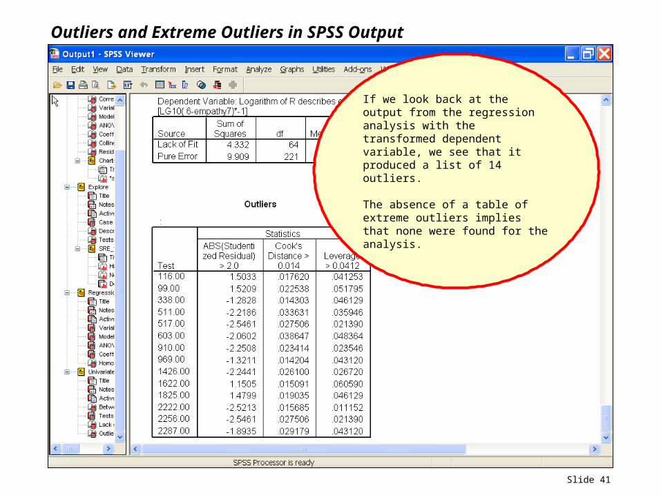
Outliers and Extreme Outliers in SPSS Output
If we look back at the output from the regression analysis with the transformed dependent variable, we see that it produced a list of 14 outliers.
The absence of a table of extreme outliers implies that none were found for the analysis.
Slide 42
Marking the Check Boxes for Regression Assumptions
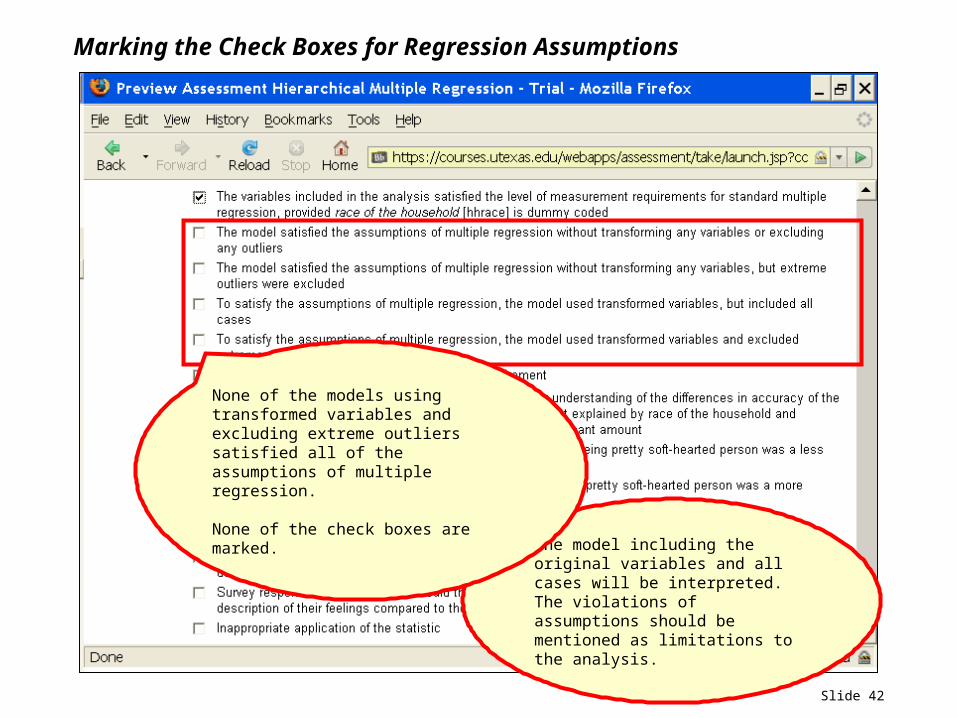
The model including the original variables and all cases will be interpreted. The violations of assumptions should be mentioned as limitations to the analysis.
None of the models using transformed variables and excluding extreme outliers satisfied all of the assumptions of multiple regression.
None of the check boxes are marked.
Slide 43
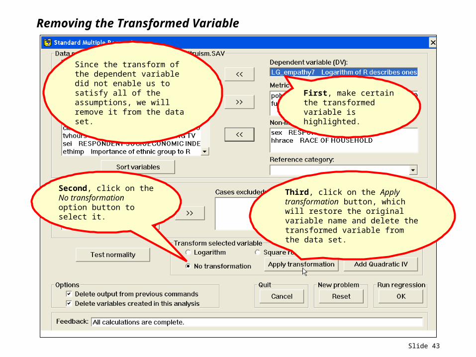
Removing the Transformed Variable
Since the transform of the dependent variable did not enable us to satisfy all of the assumptions, we will remove it from the data set.
First, make certain the transformed variable is highlighted.
Third, click on the Apply transformation button, which will restore the original variable name and delete the transformed variable from the data set.
Second, click on the No transformation option button to select it.
Slide 44
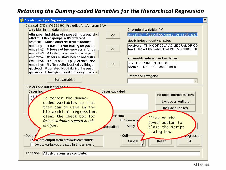
Retaining the Dummy-coded Variables for the Hierarchical Regression
To retain the dummy-coded variables so that they can be used in the hierarchical regression, clear the check box for Delete variables created in this analysis.
Click on the Cancel button to close the script dialog box.
Slide 45
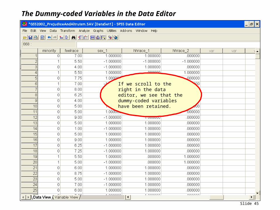
The Dummy-coded Variables in the Data Editor
If we scroll to the right in the data editor, we see that the dummy-coded variables have been retained.
Slide 46
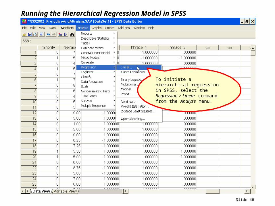
Running the Hierarchical Regression Model in SPSS
To initiate a hierarchical regression in SPSS, select the Regression > Linear command from the Analyze menu.
Slide 47
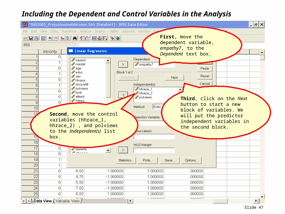
Including the Dependent and Control Variables in the Analysis
First, move the dependent variable, empathy7, to the Dependent text box.
Second, move the control variables (hhrace_1, hhrace_2) , and polviews to the Independent(s) list box.
Third, click on the Next button to start a new block of variables. We will put the predictor independent variables in the second block.
Slide 48
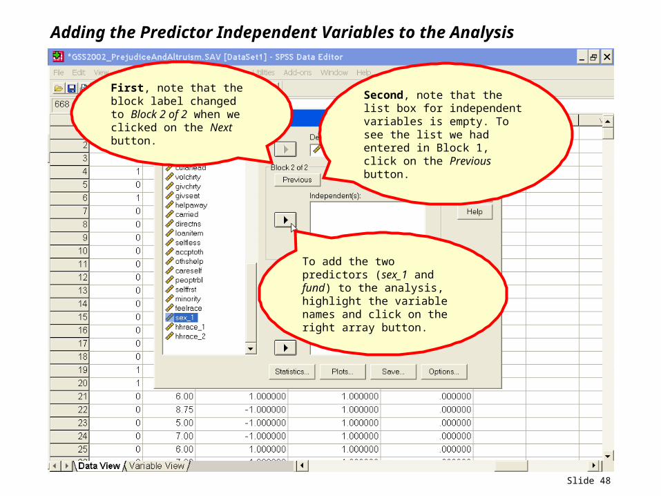
Adding the Predictor Independent Variables to the Analysis
First, note that the block label changed to Block 2 of 2 when we clicked on the Next button.
Second, note that the list box for independent variables is empty. To see the list we had entered in Block 1, click on the Previous button.
To add the two predictors (sex_1 and fund) to the analysis, highlight the variable names and click on the right array button.
Slide 49
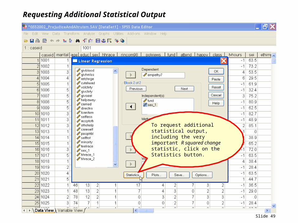
Requesting Additional Statistical Output
To request additional statistical output, including the very important R squared change statistic, click on the Statistics button.
Slide 50
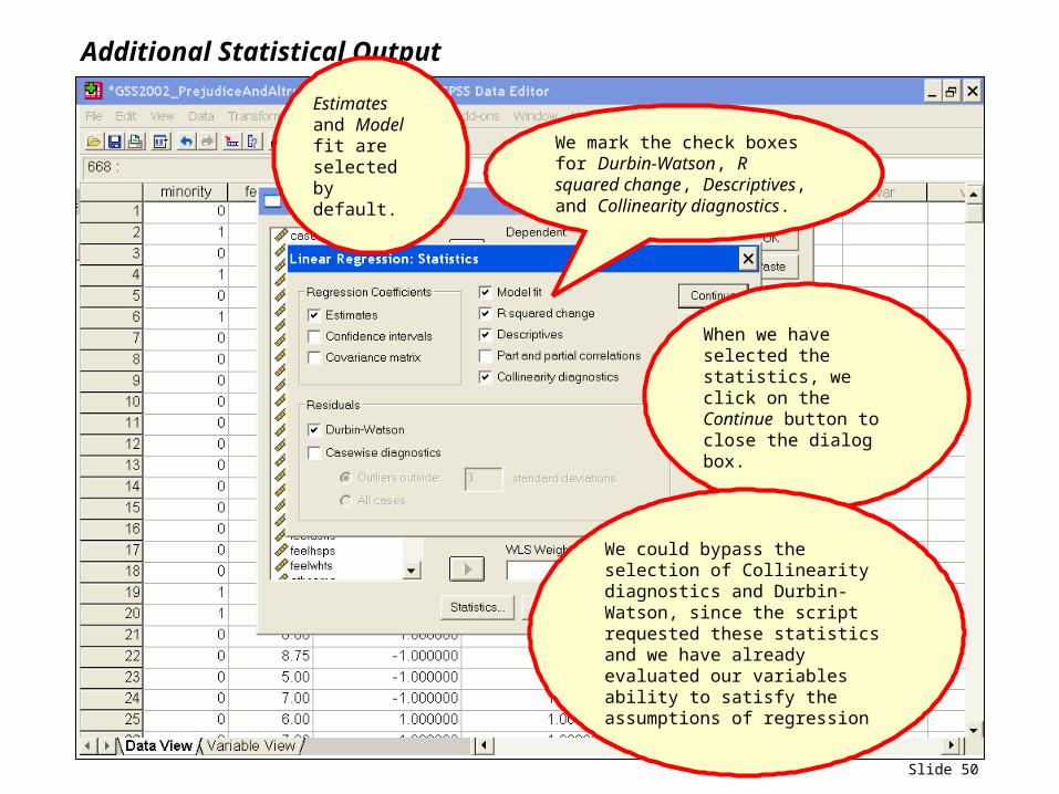
Additional Statistical Output
Estimates and Model fit are selected by default.
We mark the check boxes for Durbin-Watson, R squared change, Descriptives, and Collinearity diagnostics.
When we have selected the statistics, we click on the Continue button to close the dialog box.
We could bypass the selection of Collinearity diagnostics and Durbin-Watson, since the script requested these statistics and we have already evaluated our variables ability to satisfy the assumptions of regression
Slide 51
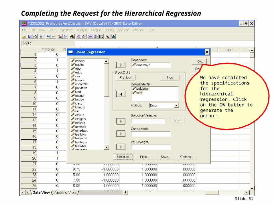
Completing the Request for the Hierarchical Regression
We have completed the specifications for the hierarchical regression. Click on the OK button to generate the output.
Slide 52
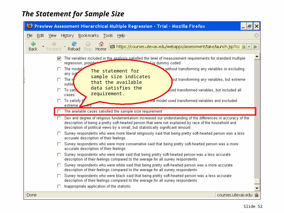
The Statement for Sample Size
The statement for sample size indicates that the available data satisfies the requirement.
Slide 53
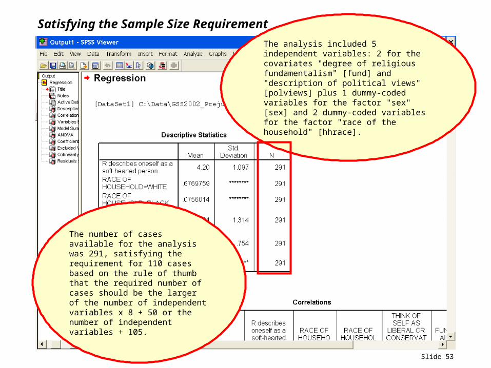
Satisfying the Sample Size Requirement
The number of cases available for the analysis was 291, satisfying the requirement for 110 cases based on the rule of thumb that the required number of cases should be the larger of the number of independent variables x 8 + 50 or the number of independent variables + 105.
The analysis included 5 independent variables: 2 for the covariates "degree of religious fundamentalism" [fund] and "description of political views" [polviews] plus 1 dummy-coded variables for the factor "sex" [sex] and 2 dummy-coded variables for the factor "race of the household" [hhrace].
Slide 54
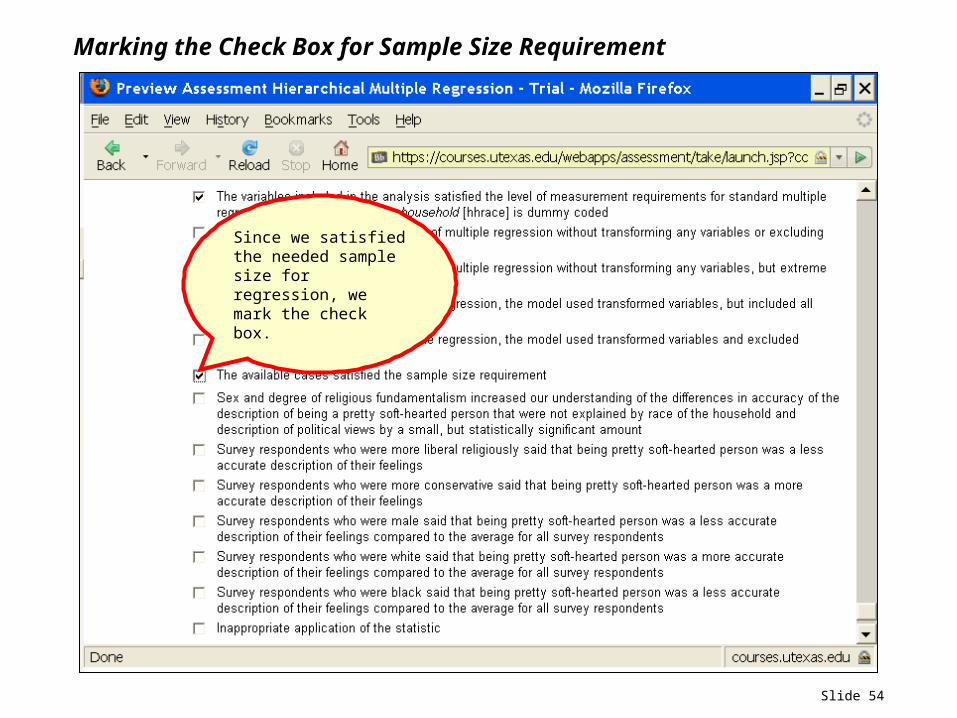
Marking the Check Box for Sample Size Requirement
Since we satisfied the needed sample size for regression, we mark the check box.
Slide 55
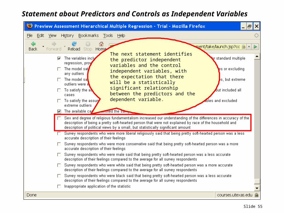
Statement about Predictors and Controls as Independent Variables
The next statement identifies the predictor independent variables and the control independent variables, with the expectation that there will be a statistically significant relationship between the predictors and the dependent variable.
Slide 56
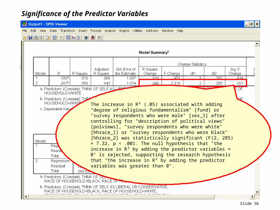
Significance of the Predictor Variables
The increase in R² (.05) associated with adding "degree of religious fundamentalism" [fund] or "survey respondents who were male" [sex_1] after controlling for "description of political views" [polviews], "survey respondents who were white" [hhrace_1] or "survey respondents who were black" [hhrace_2] was statistically significant (F(2, 285) = 7.32, p < .001. The null hypothesis that "the increase in R² by adding the predictor variables = 0" is rejected, supporting the research hypothesis that "the increase in R² by adding the predictor variables was greater than 0".
Slide 57
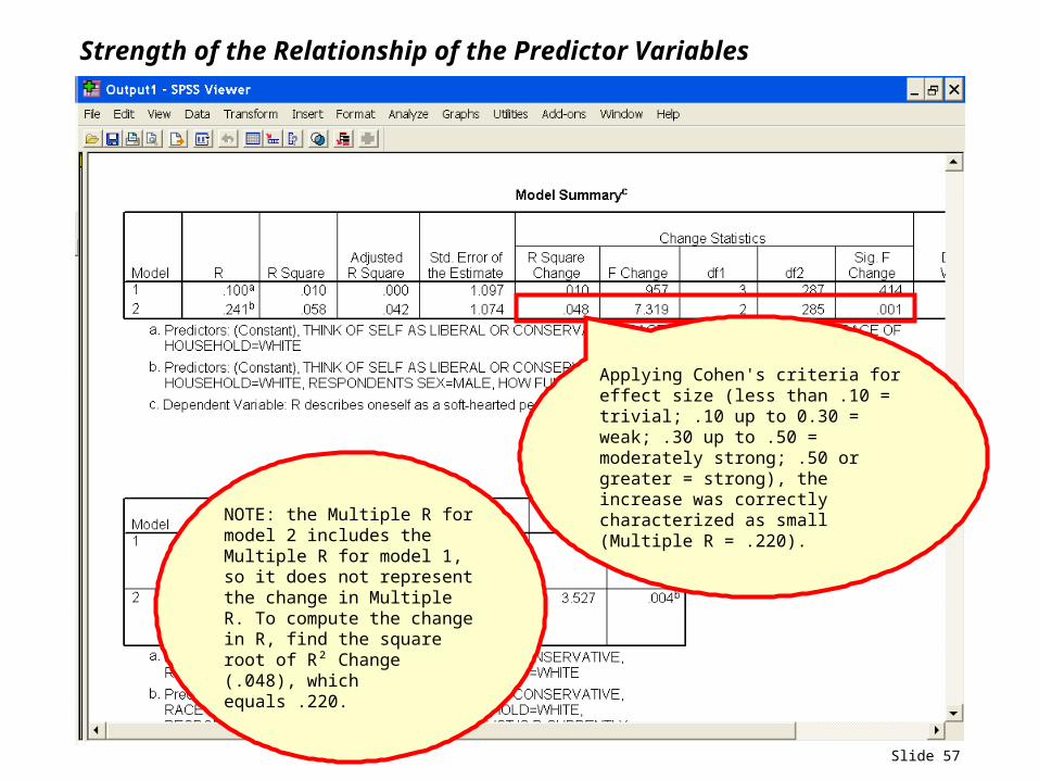
Strength of the Relationship of the Predictor Variables
Applying Cohen's criteria for effect size (less than .10 = trivial; .10 up to 0.30 = weak; .30 up to .50 = moderately strong; .50 or greater = strong), the increase was correctly characterized as small (Multiple R = .220).NOTE: the Multiple R for
model 2 includes the Multiple R for model 1, so it does not represent the change in Multiple R. To compute the change in R, find the square root of R² Change (.048), which equals .220.
Slide 58
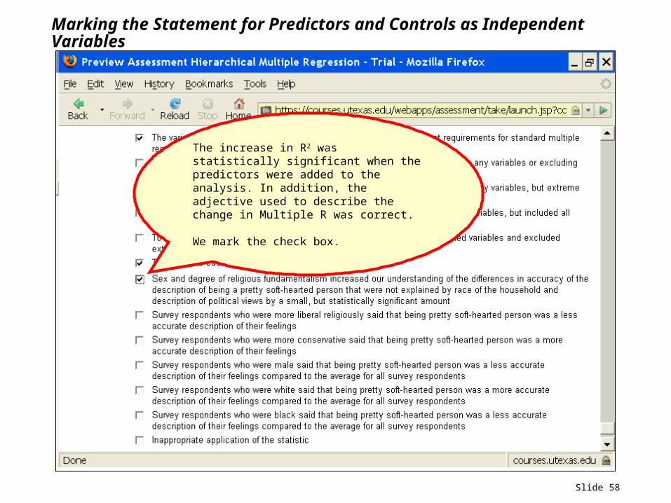
Marking the Statement for Predictors and Controls as Independent Variables
The increase in R2 was statistically significant when the predictors were added to the analysis. In addition, the adjective used to describe the change in Multiple R was correct. We mark the check box.
Slide 59
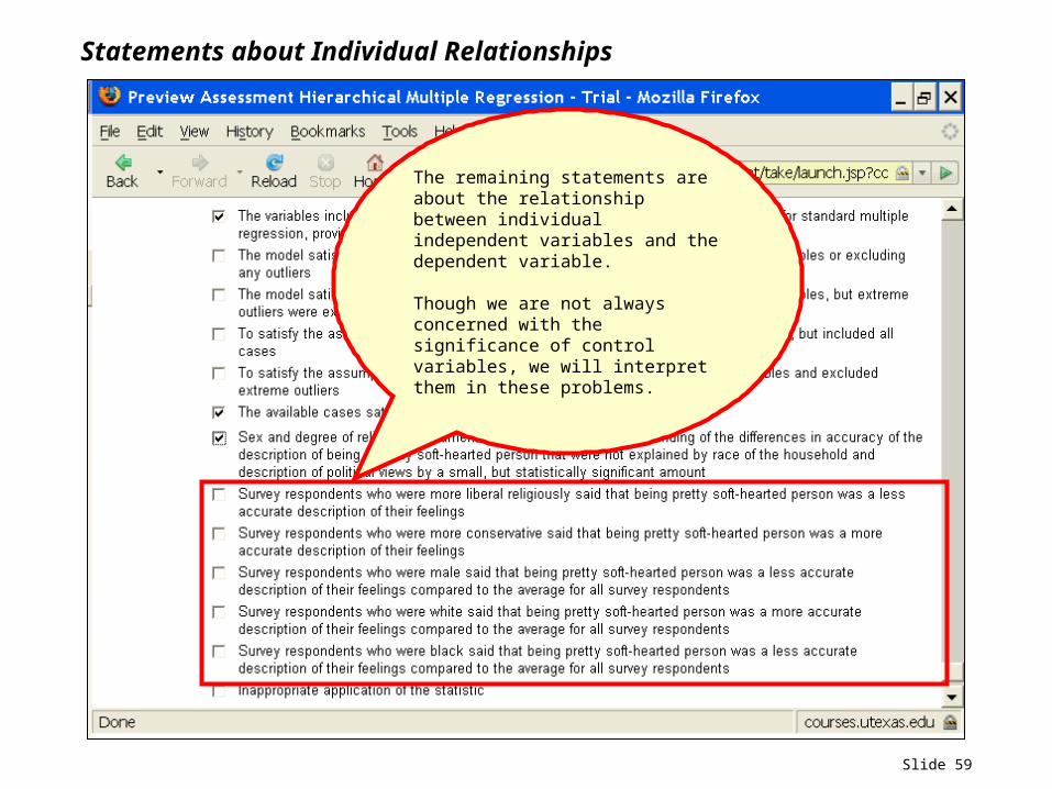
Statements about Individual Relationships
The remaining statements are about the relationship between individual independent variables and the dependent variable.
Though we are not always concerned with the significance of control variables, we will interpret them in these problems.

Slide 60
Statements about Individual Relationships
The first statement focuses on the relationship between religious fundamentalism and empathy.
Slide 61
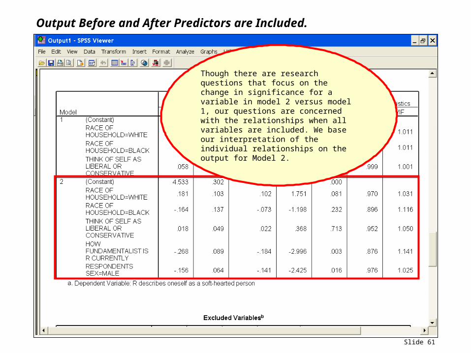
Output Before and After Predictors are Included.
Though there are research questions that focus on the change in significance for a variable in model 2 versus model 1, our questions are concerned with the relationships when all variables are included. We base our interpretation of the individual relationships on the output for Model 2.
Slide 62
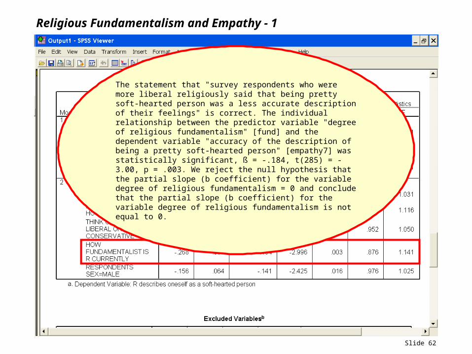
Religious Fundamentalism and Empathy - 1
The statement that "survey respondents who were more liberal religiously said that being pretty soft-hearted person was a less accurate description of their feelings" is correct. The individual relationship between the predictor variable "degree of religious fundamentalism" [fund] and the dependent variable "accuracy of the description of being a pretty soft-hearted person" [empathy7] was statistically significant, ß = -.184, t(285) = -3.00, p = .003. We reject the null hypothesis that the partial slope (b coefficient) for the variable degree of religious fundamentalism = 0 and conclude that the partial slope (b coefficient) for the variable degree of religious fundamentalism is not equal to 0.
Slide 63
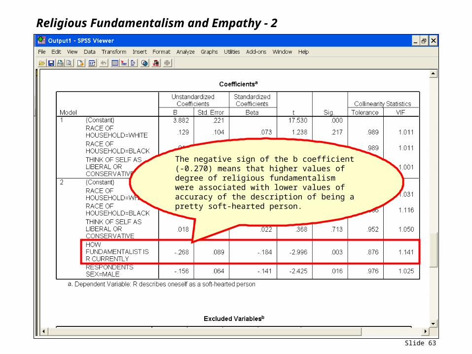
Religious Fundamentalism and Empathy - 2
The negative sign of the b coefficient (-0.270) means that higher values of degree of religious fundamentalism were associated with lower values of accuracy of the description of being a pretty soft-hearted person.
Slide 64
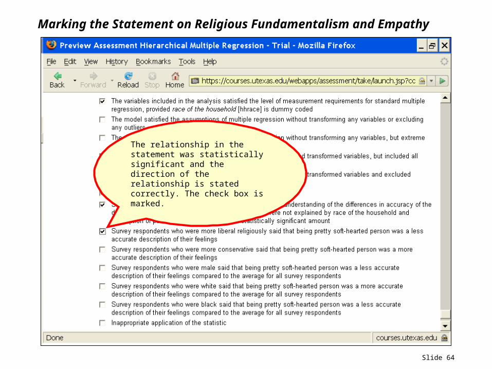
Marking the Statement on Religious Fundamentalism and Empathy
The relationship in the statement was statistically significant and the direction of the relationship is stated correctly. The check box is marked.
Slide 65
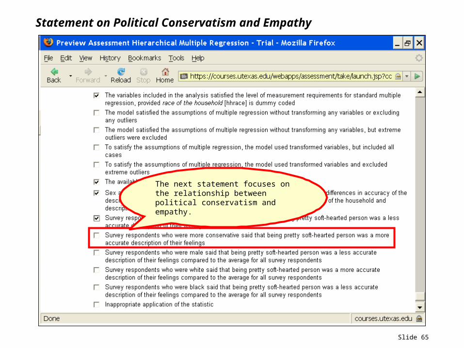
Statement on Political Conservatism and Empathy
The next statement focuses on the relationship between political conservatism and empathy.
Slide 66
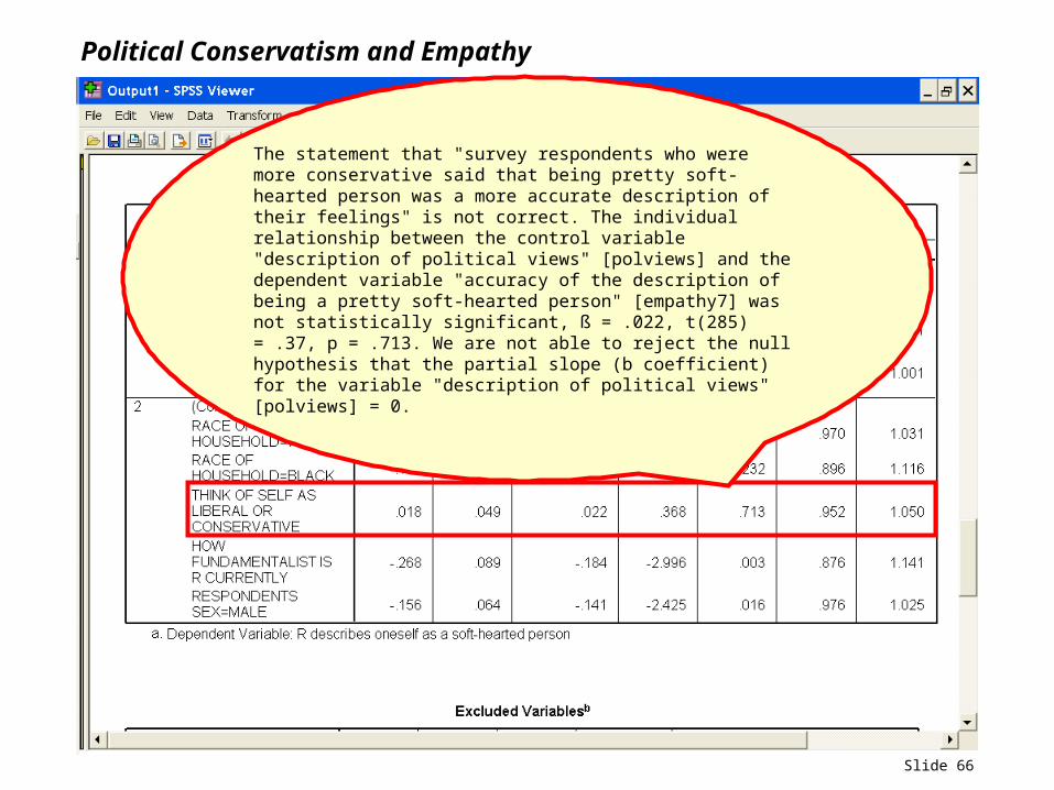
Political Conservatism and Empathy
The statement that "survey respondents who were more conservative said that being pretty soft-hearted person was a more accurate description of their feelings" is not correct. The individual relationship between the control variable "description of political views" [polviews] and the dependent variable "accuracy of the description of being a pretty soft-hearted person" [empathy7] was not statistically significant, ß = .022, t(285) = .37, p = .713. We are not able to reject the null hypothesis that the partial slope (b coefficient) for the variable "description of political views" [polviews] = 0.
Slide 67
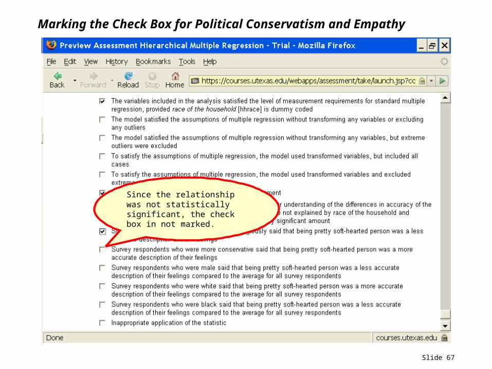
Marking the Check Box for Political Conservatism and Empathy
Since the relationship was not statistically significant, the check box in not marked.
Slide 68
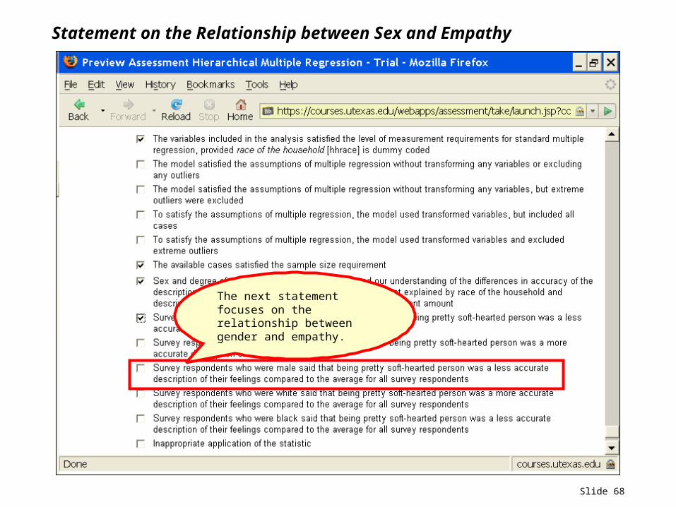
Statement on the Relationship between Sex and Empathy
The next statement focuses on the relationship between gender and empathy.
Slide 69
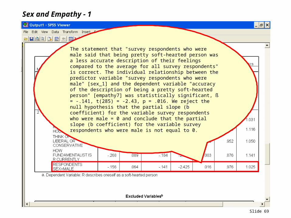
Sex and Empathy - 1
The statement that "survey respondents who were male said that being pretty soft-hearted person was a less accurate description of their feelings compared to the average for all survey respondents" is correct. The individual relationship between the predictor variable "survey respondents who were male" [sex_1] and the dependent variable "accuracy of the description of being a pretty soft-hearted person" [empathy7] was statistically significant, ß = -.141, t(285) = -2.43, p = .016. We reject the null hypothesis that the partial slope (b coefficient) for the variable survey respondents who were male = 0 and conclude that the partial slope (b coefficient) for the variable survey respondents who were male is not equal to 0.
Slide 70
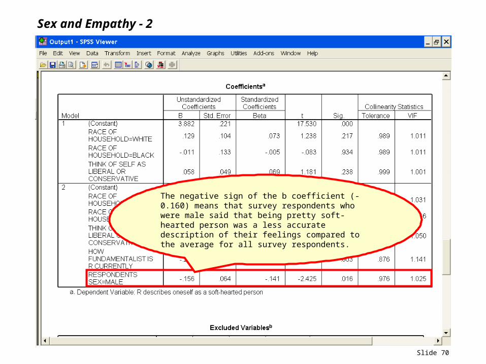
Sex and Empathy - 2
The negative sign of the b coefficient (-0.160) means that survey respondents who were male said that being pretty soft-hearted person was a less accurate description of their feelings compared to the average for all survey respondents.
Slide 71
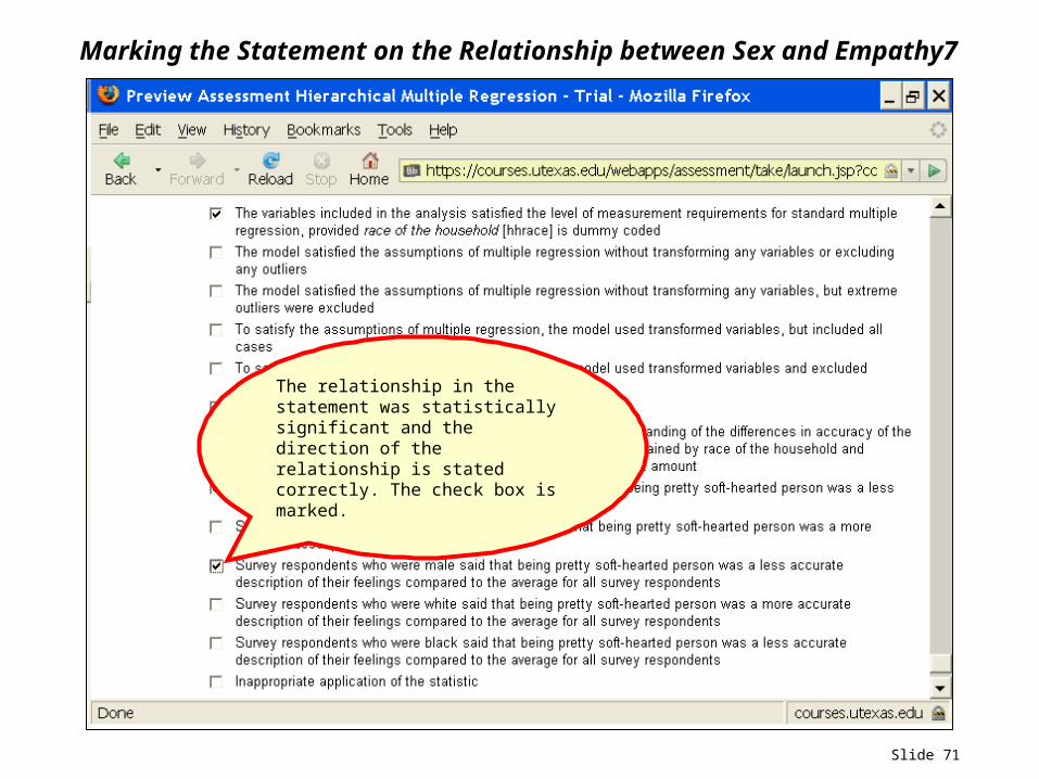
Marking the Statement on the Relationship between Sex and Empathy7
The relationship in the statement was statistically significant and the direction of the relationship is stated correctly. The check box is marked.
Slide 72
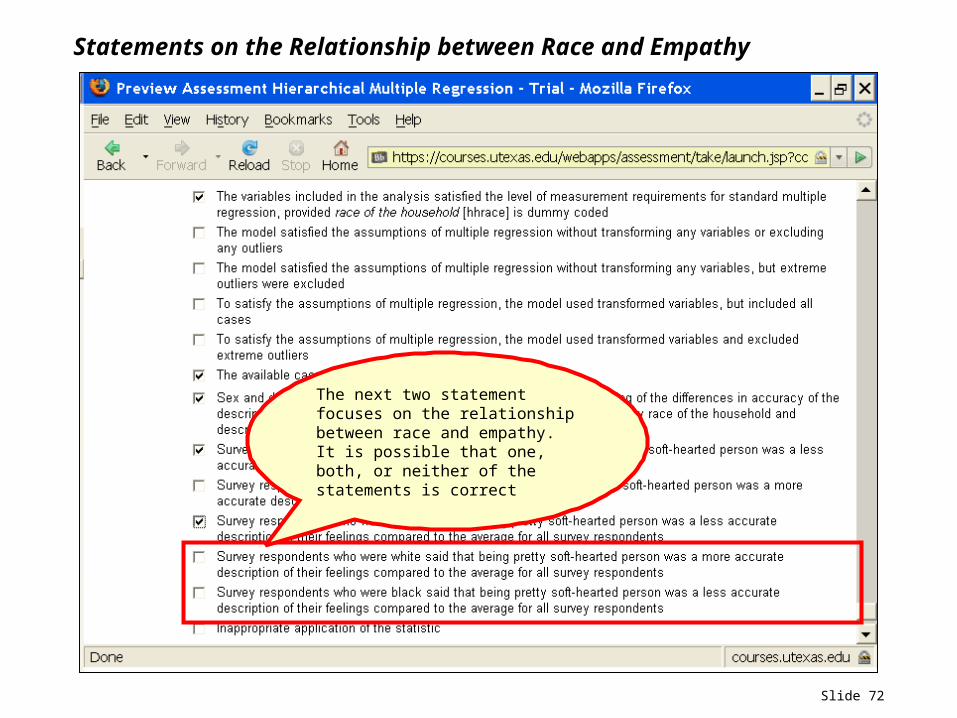
Statements on the Relationship between Race and Empathy
The next two statement focuses on the relationship between race and empathy. It is possible that one, both, or neither of the statements is correct
Slide 73
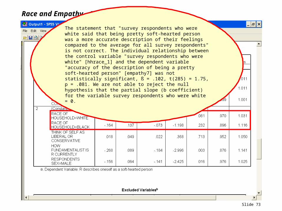
Race and Empathy - 1
The statement that "survey respondents who were white said that being pretty soft-hearted person was a more accurate description of their feelings compared to the average for all survey respondents" is not correct. The individual relationship between the control variable "survey respondents who were white" [hhrace_1] and the dependent variable "accuracy of the description of being a pretty soft-hearted person" [empathy7] was not statistically significant, ß = .102, t(285) = 1.75, p = .081. We are not able to reject the null hypothesis that the partial slope (b coefficient) for the variable survey respondents who were white = 0.
Slide 74
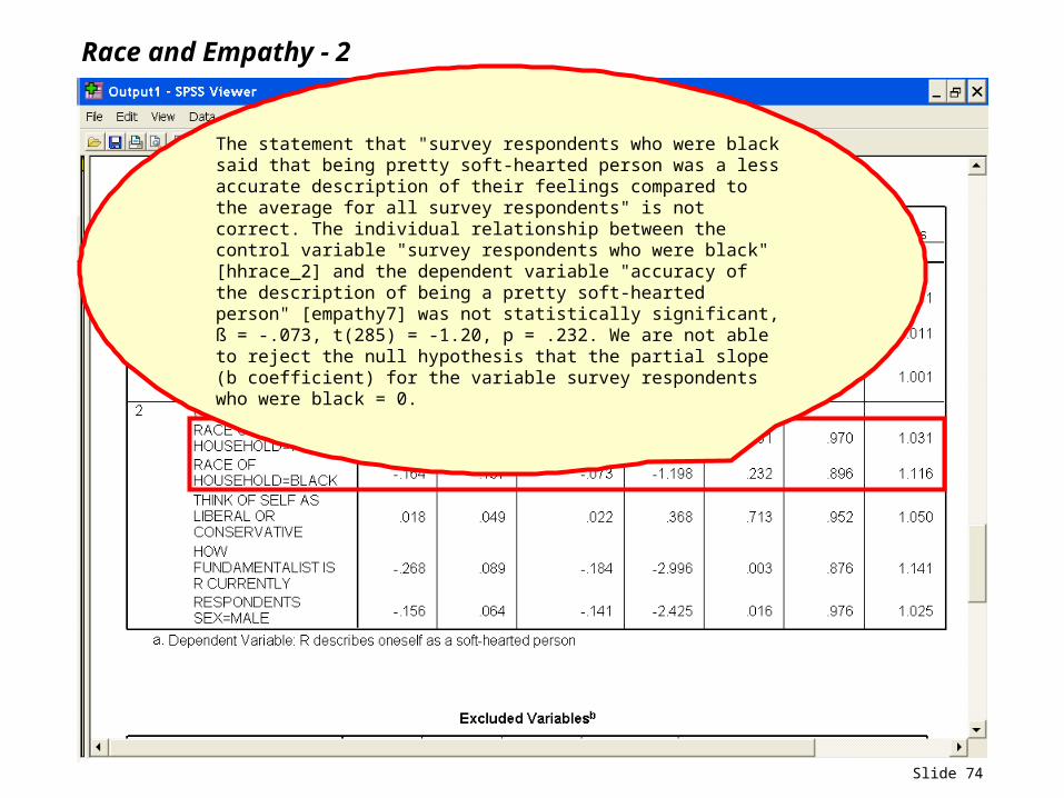
Race and Empathy - 2
The statement that "survey respondents who were black said that being pretty soft-hearted person was a less accurate description of their feelings compared to the average for all survey respondents" is not correct. The individual relationship between the control variable "survey respondents who were black" [hhrace_2] and the dependent variable "accuracy of the description of being a pretty soft-hearted person" [empathy7] was not statistically significant, ß = -.073, t(285) = -1.20, p = .232. We are not able to reject the null hypothesis that the partial slope (b coefficient) for the variable survey respondents who were black = 0.
Slide 75
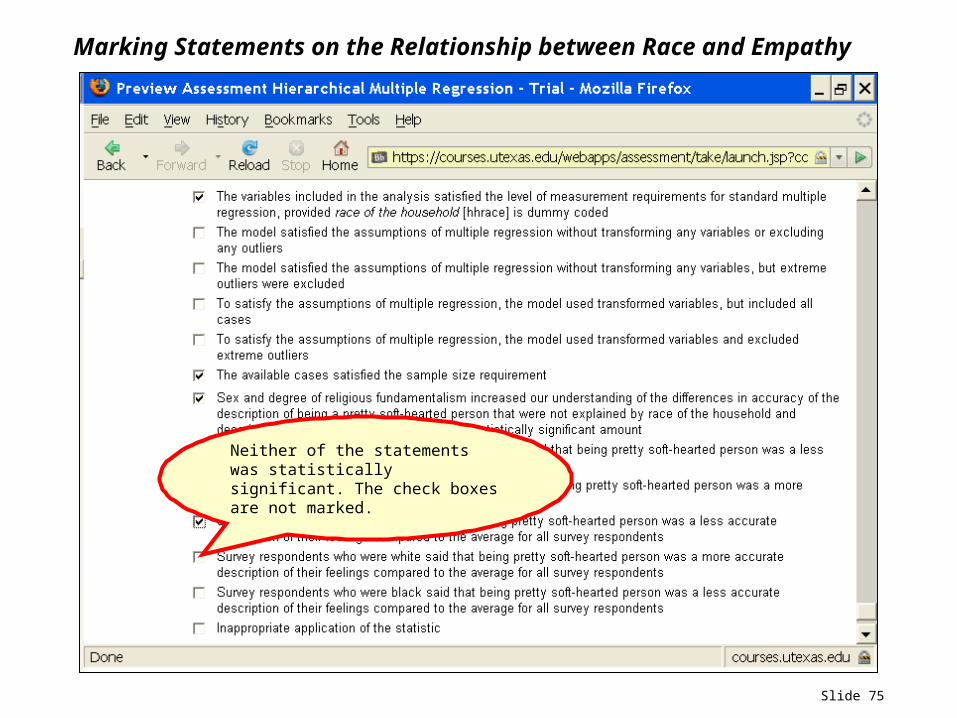
Marking Statements on the Relationship between Race and Empathy
Neither of the statements was statistically significant. The check boxes are not marked.
Slide 76
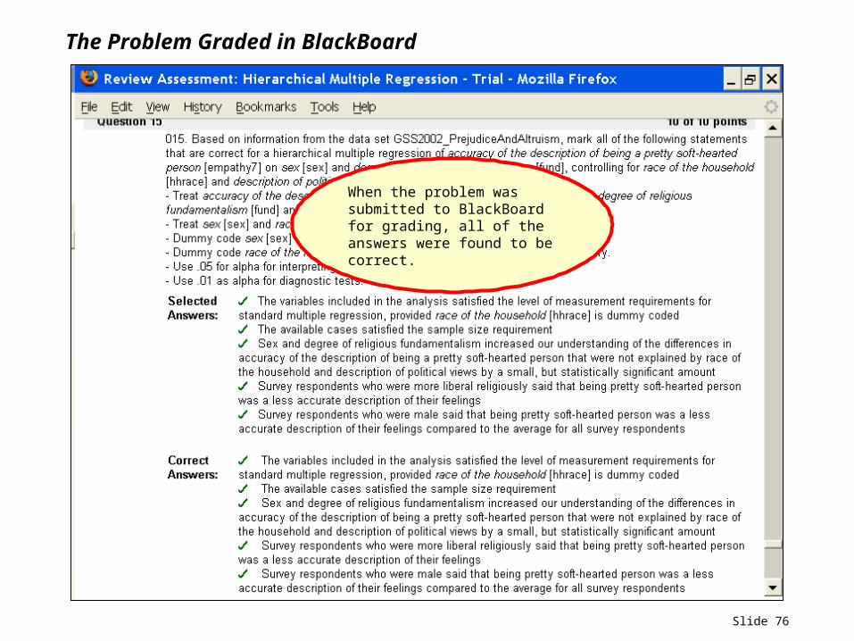
The Problem Graded in BlackBoard
When the problem was submitted to BlackBoard for grading, all of the answers were found to be correct.
Slide 77
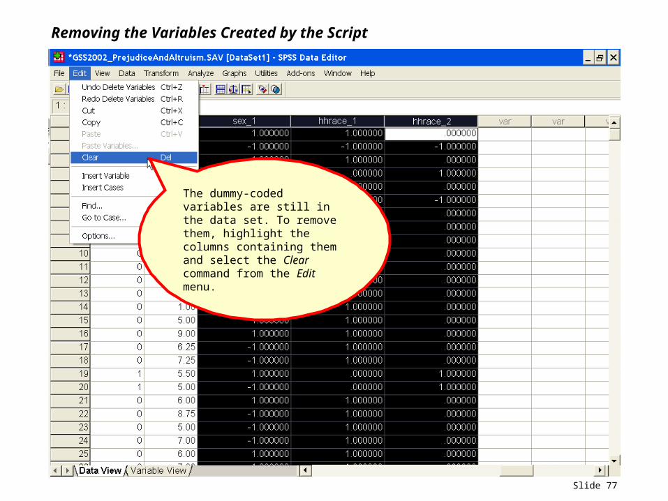
Removing the Variables Created by the Script
The dummy-coded variables are still in the data set. To remove them, highlight the columns containing them and select the Clear command from the Edit menu.
Slide 78
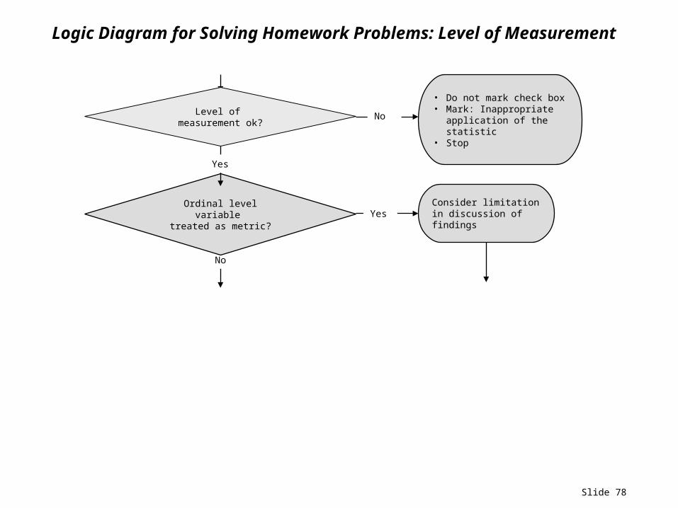
Logic Diagram for Solving Homework Problems: Level of Measurement
No
No
Ordinal level variable treated as metric?
• Do not mark check box• Mark: Inappropriate
application of the statistic
• Stop
Yes
Yes
Level of measurement ok?
Consider limitation in discussion of findings
Slide 79
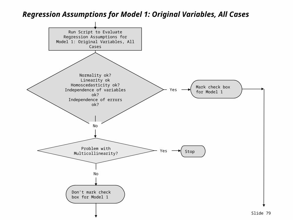
Regression Assumptions for Model 1: Original Variables, All Cases
Run Script to Evaluate Regression Assumptions for
Model 1: Original Variables, All Cases
Mark check box for Model 1
Don’t mark check box for Model 1
Normality ok?Linearity ok
Homoscedasticity ok? Independence of variables ok?
Independence of errors ok?
No
Yes
Problem with Multicollinearity?
No
Yes Stop

Slide 80
Regression Assumptions for Model 2: Original Variables, Excluding Extreme Outliers
Run Script to Evaluate Regression Assumptions for Model 2: Original Variables, Excluding Extreme Outliers
Mark check box for Model 2
Don’t mark check box for Model 2
Normality ok?Linearity ok
Homoscedasticity ok? Independence of variables ok?
Independence of errors ok?
No
Yes
If no extreme outliers are identified in Model 1, skip this step
Problem with Multicollinearity?
No
Yes Stop
Slide 81
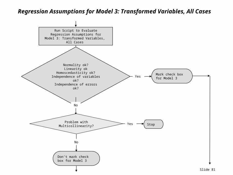
Regression Assumptions for Model 3: Transformed Variables, All Cases
Run Script to Evaluate Regression Assumptions for
Model 3: Transformed Variables, All Cases
Mark check box for Model 3
Don’t mark check box for Model 3
Normality ok?Linearity ok
Homoscedasticity ok? Independence of variables ok?
Independence of errors ok?
No
Yes
Problem with Multicollinearity?
No
Yes Stop
Slide 82
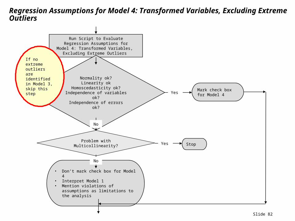
Regression Assumptions for Model 4: Transformed Variables, Excluding Extreme Outliers
Run Script to Evaluate Regression Assumptions for
Model 4: Transformed Variables, Excluding Extreme Outliers
Mark check box for Model 4
Normality ok?Linearity ok
Homoscedasticity ok? Independence of variables ok?
Independence of errors ok?
No
Yes
If no extreme outliers are identified in Model 3, skip this step
• Don’t mark check box for Model 4• Interpret Model 1• Mention violations of assumptions
as limitations to the analysis
Problem with Multicollinearity? Yes Stop
No
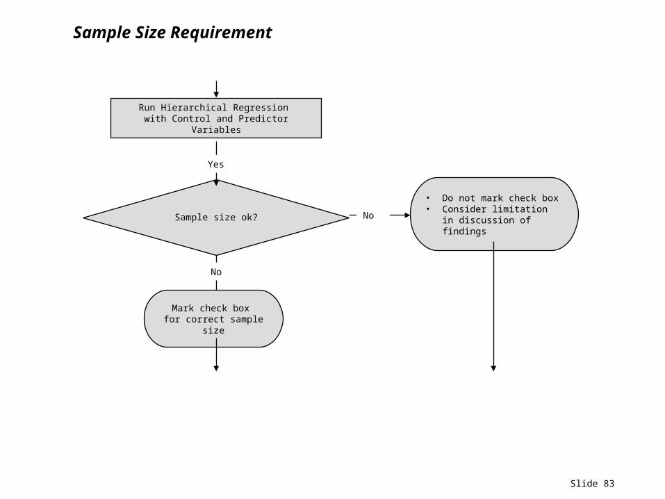
Slide 83
Sample Size Requirement
• Do not mark check box• Consider limitation in
discussion of findings
No
Sample size ok? No
Yes
Mark check box for correct sample size
Run Hierarchical Regression with Control and Predictor
Variables
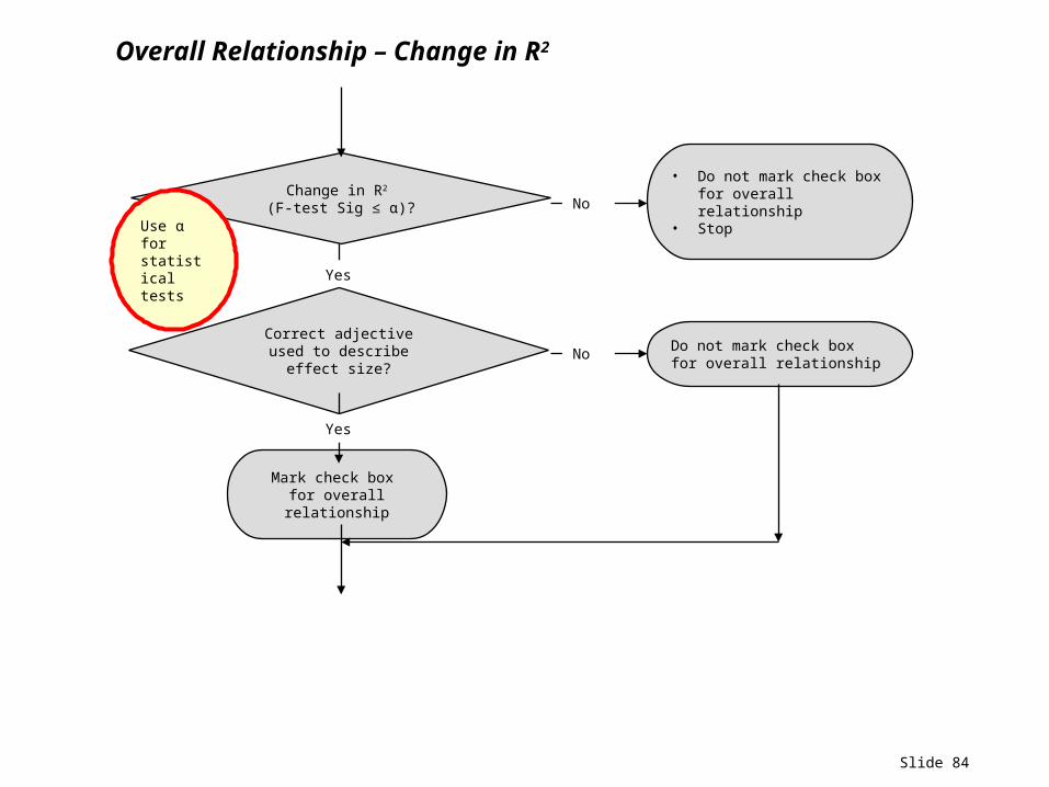
Slide 84
Overall Relationship – Change in R2
Yes
• Do not mark check box for overall relationship
• Stop
Change in R2 (F-test Sig ≤ α)? No
Mark check box for overall relationship
Use α for statistical tests
Correct adjective used to describe effect size?
Yes
Do not mark check box for overall relationship
No
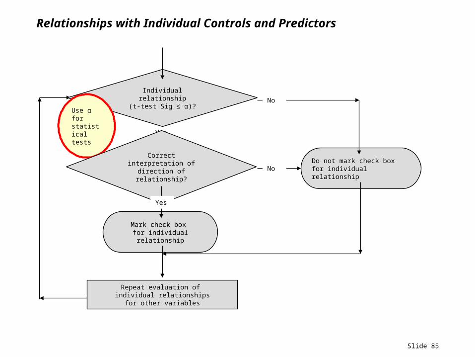
Slide 85
Relationships with Individual Controls and Predictors
Yes
Individual relationship(t-test Sig ≤ α)? No
Mark check box for individual relationship
Use α for statistical tests
Correct interpretation of direction of relationship?
Yes
Do not mark check box for individual relationship
No
Repeat evaluation of individual relationships
for other variables