sl-08-013 transient simulation of airflow and pollutant ... · ashrae transactions 131 pollutants...

Transient Simulationof Airflow and Pollutant Dispersion Under Mixing Flow and Buoyancy DrivenFlow Regimes in Residential BuildingsDonghyun Rim Atila Novoselac, PhDStudent Member ASHRAE Associate Member ASHRAE

SL-08-013

©2008. American Society of Heating, Refrigerating and Air-Conditioning Engineers, Inc. (www.ashrae.org). Published in ASHRAE Transactions, Vol. 114, Part 2. For personal use only. Additional reproduction, distribution, or transmission in either print or digital form is not permitted without ASHRAE’s prior written permission.

ABSTRACT

The distribution of airflow in a residential building varieswith the periodic operation of a heating, ventilating and air-conditioning (HVAC) system. Depending on the HVAC fanoperation, mixing airflow (fan ON) or stratified airflow (fanOFF) occurs in the space. The objectives of this study are 1)to examine the time needed for room air to stabilize after acentral ventilation fan turns ON/OFF and 2) to evaluate howthe difference in distribution of gaseous and particulate pollut-ants in the space depends on fan operation mode. In the study,experiments measured the spatial distribution of airflow andpollutant concentrations in a full-scale environmental cham-ber. The measured data then provided the basis to establish areliable computational fluid dynamics (CFD) model, whichinvestigated the concentrations of gaseous and particulatepollutants depending on the mechanical fan operation mode.The results indicate that the transition between mixing flowand stratified flow occurs in a time scale of seconds, implyingthat the airflow in residential buildings is primarily mixing orstratified flow. The results show little spatial variation of tracergas and particles in the mixing flow regime, whereas largertemporal and spatial variations are present in stratified flow.Additionally, the variations in particle concentrations arehigher than those in gaseous concentrations. In certain areasof the room the particle concentration with stratified flow is upto thirty times higher than that with mixing flow, implying ahigh potential of exposure to particles when the fan is OFF.

INTRODUCTION

Thermal comfort and level of exposure to indoor pollut-ants vary with airflow pattern in an occupied space (Novoselacand Sebric 2002; Zhao et al. 2004; Bouilly 2005). In residen-

tial buildings, where periodic operation of air-conditioningsystems occurs, the indoor airflow pattern mainly depends onthe mechanical operation of the fan and the presence of heatsources. During fan operation, forced convection often domi-nates over the buoyant airflow generated by indoor heatsources, which creates a mixing flow regime in the space.However, when the fan is off, buoyant thermal plumes fromindoor heat sources become dominant, causing buoyancydriven flow.

Given that the transport of indoor pollutants is directlyrelated to the airflow distribution in the space (Lin et al. 2005;Gao and Liu 2007; Li et. al 2007), the mixing and buoyantairflows each have distinct effects on the transport of indoorairborne pollutants. With the mixing airflow, the largemomentum of supply air scatters pollutants through the space,providing more or less uniform distribution of pollutants.Conversely, in a room with buoyancy driven airflow, theindoor heat sources raise the air to upper level of the space,causing thermal stratification and non-uniform pollutantconcentrations in the space.

On average, residential buildings operate their HVAC fans17% of the day (Ward et al. 2005). Consequently, both mixingairflow and buoyant airflow periodically exist in residential build-ings. Previous studies have investigated how pollutants transportunder mixing flow and buoyancy driven flow regimes. In thesestudies, researchers often used displacement ventilation to createbuoyant airflow from indoor heat sources. Huang et al. (2004)conducted a numerical study of exposure to household contami-nants, including carbon dioxide and carbon monoxide, in asingle-family house with different airflow patterns. They reportedlower occupant exposure with buoyant flow than with mixingflow. Lin et al. (2005) measured the concentrations of gaseous

130 ©2008 ASHRAE

Donghyun Rim is a doctoral student and Atila Novoselac is an assistant professor in the Department of Civil, Architectural and EnvironmentalEngineering, The University of Texas at Austin, TX.

pollutants such as carbon monoxide and different VOCs withmixing and displacement ventilation in offices, industrial work-shops, and public places. They concluded that the buoyant airflowassociated with displacement ventilation provides better indoorair quality in the breathing zone than mixing ventilation. He et al.(2005) used a validated computer model to examine dispersion ofa gaseous pollutant (SF6) emitted from a floor surface and foundthat concentration stratification exists with displacement ventila-tion. Considering particles (1~10 µm) that enter the space withsupply air (by infiltration or ventilation), Gao and Liu (2007)found lower exposure for occupants in the room with air mixingthan in the room with buoyant flow. Taken together, these previ-ous research results suggest that indoor airflow pattern and airmixing associated with operating ventilation fans could havesignificant impact on pollutant transport and occupant exposurein residential buildings.

The studies in literature extensively examined the airflowand pollutant concentration variations with airflow patterns.However, the previous studies all lack information on the tran-sition period between the mixing flow regime and the buoy-ancy driven flow regime. The transition between mixing flowand buoyant flow occurs frequently in residential buildingssince periodic operation of fan is common. In addition, themajority of previous studies focused on pollutant concentra-tions due to steady source emissions. However, transientpollutant transport, such as a short release of pollutant in anoccupied space, may be the more common and relevant prob-lem. Examples of transient contaminant release are combus-tion sources and particle re-suspension from surfaces createdby different indoor activities.

The objectives of this study were as follows:

1. Examine the time needed for room airflow to stabilizeafter a central residential fan turns ON/OFF

2. Evaluate the effects of airflow distribution on spatial andtemporal concentrations of gaseous and particulatepollutants emitted from a source which is active for ashort-time period.

Experiments in a full scale environmental chamber wereconducted to measure the airflow dynamics due to residentialfan usage. The experiments were used to validate numericalsimulations that determined the pollutant distribution in thespace for different fan operations. The following sections willbe presented in the following order: airflow dynamics withventilation fan operation, experimental validation of numeri-cal models for unsteady-state contaminant flow analysis, andprediction of pollutant distribution in a room using the vali-dated numerical model.

AIRFLOW DYNAMICS WITH RESIDENTIAL FAN OPERATION

The first set of experiments measured air flow velocitymagnitudes for two fan operation modes: fan ON and fan OFF.To analyze the transition of airflow from mixing flow to buoy-ancy driven flow and vice versa, an environmental chamber ofvolume 67 m3 (2366 ft3) with a thermal manikin was used. Theenvironmental chamber was equipped with an air handlingunit (AHU), which controlled and monitored the supplyairflow rate, temperature and humidity of the air in the room.The manikin had an accurate geometrical similarity to a realperson and the electric heaters inside the skin shell generatedheat flux in each part of the body.

Experimental Setup

Figure 1 shows the experimental setup for monitoring airspeed at characteristic points in the space with intermittent fanoperation. The experimental setup in the environmental cham-ber represents a typical residential room. A thermal manikinwhich simulates a human presence was placed in the center ofthe chamber (Figure 1a). The manikin had a total heat flux of90W across the skin and cloth surfaces. The convectiveportion of this flux created a buoyant thermal plume in thevicinity of the manikin. In addition, indoor heat sources, suchas sun patches on the floor and heat sources such as TVs or

(a) (b)

Figure 1 Experimental setup for analyses of effects of fan operation, with (a) being a schematic diagram of experiment, and(b) being a manikan and velocity sensors.

ASHRAE Transactions 131

computers, were distributed in the chamber to simulate theenvironment typical for a residential space (Figure 1b).

To simulate a residential room when the mechanicalventilation is OFF and only infiltration is present, supply airwas provided with low speed. In this case the airflow in thespace was driven primarily by buoyancy from indoor heatsources. A mixing fan in the space was used to convert buoyantflow to mixing flow. The power and position of the fan wereadjusted to generate forced convection typical for a residentialspace with the air-conditioning system working. The transi-tion of the airflow field between buoyant flow and mixing flowand vice versa was analyzed by examining the transient airspeed in the space for intermittent operation of the mixing fan.

Spatial distribution of air speed was measured usingomni-directional low velocity sensors, which measure meanvelocity magnitude. The airflow direction was determinedusing smoke visualization tests. The airflow data werecollected at 16 positions in space. The analysis in this paperwill focus on the two characteristic points: (1) the location 25cm (9.8 in) above the manikin head (V1) and (2) the locationin the stagnation zone in the room (V2), as shown in Figure 1a.The selection of the two monitoring points was based on astudy by Murakami et al. (1997), which analyzed the boundarylayer of the thermal plume around a human body. They foundthat in a room with still air the thermal boundary layer at footlevel is about 5 cm (2.0 in) thick and around the neck 19 cm(7.7 in). In our experiment, the monitoring point in the stag-nation zone (V2) was located at a distance of approximately60cm (24 in) from the manikin.

Airflow intensity is the largest above the thermal manikindue to the effects of buoyant forces from the whole body. Theair speed above the head (V1) represents the strength of theplume. On the other hand the air speed in the stagnation zone(V2) illustrates the effects of momentum forces induced by thefan. When the fan operates, the air velocities in the vicinity ofchamber surfaces ranged from 0.5 - 2.5 m/s (1.6-8.2 ft/s), andthe velocities in the central spaces were in the range 0.15-0.25m/s (0.49-0.82 ft/s). To investigate the transition period fromthe buoyant airflow to the mixing flow, the fan operation wasintermittent with several minutes of ON and OFF periods.

Room Airflow Dynamics with Intermittent Operation of Ventilation Fan

The experiments applied intermittent fan operation typi-cal of residential air-conditioning systems. Figure 2 shows thevelocity magnitudes at V1 (above the head) and at V2 (stag-nation zone) for the two different fan operation modes. Whenthe fan was OFF, the ambient airflow velocity at V2 (stagna-tion zone) does not fluctuate, indicating that the ambientairflow is not affected by the buoyant thermal plume. Also, theaverage velocity magnitudes at V1 (above the head) and at V2(stagnation zone) are 0.19 m/s (0.62 ft/s) and 0.03 m/s (0.10ft/s), respectively, and this six-fold difference in velocity is dueto the thermal plume above the head. With the fan OFF, thedifference between velocity magnitudes at V1 (above the

head) and at V2 (stagnation zone) was decreased, as shown inFigure 2. With the operation of the fan, a significant air mixingoccurs and the buoyant thermal plume in the space is disturbedby the mixing flow. Figure 2 indicates that the duration of thetransient period between the two operation modes (fan ON andfan OFF) is approximately one minute.

Thus, the operation of a fan operation affects airflow inthe vicinity of a buoyant plume and in the entire space. Whenthe fan operates, intensive air mixing occurs, disrupting thebuoyant airflow. The experimental data demonstrate that thetransition time between the two fan operation modes is rela-tively short (approximately 60 seconds) compared to fan oper-ating or non-operating period. This result implies that,depending on the fan operation, the airflow in a residentialbuilding is primarily mixing flow or buoyant driven flow, notin a transition state between the two. The mixing and buoyantairflow patterns have different characteristics in air speed,turbulence intensity, and mixing intensity. Accordingly, thetwo different airflow patterns could have distinct effects on thepollutant transport, dispersion and removal in the space. Thefollowing sections will examine pollutant distribution andoccupant exposure associated with the two major airflowpatterns in residence.

POLLUTANT TRANSPORT ASSOCIATED WITH RESIDENTIAL FAN OPERATION

The second part of the study investigated the effects of theresidential fan operation on the transport of gaseous andparticulate pollutants in three stages. First, experimentsmeasured temporal and spatial concentrations of gaseous andparticulate pollutants with a short-term point source release.Second, by using the mock-up test results, the study estab-lished and validated a CFD model to accurately predict the

Figure 2 Velocity magnitudes at two sampling points(above head and stagnation zone) with two fanoperation modes: fan ON and fan OFF.

132 ASHRAE Transactions

transient pollutant concentrations. Third, the validated CFDmodel was further used to investigate spatial and temporalpollutant concentrations with the two characteristic airflowregimes: (1) mixing flow (fan ON) and (2) buoyancy drivenflow (fan OFF).

Mock-Up Experiments to Validate CFD Model

The experiments with the buoyancy driven flow wereused to develop high quality mock-up tests, given the chal-lenges in modeling the varied level of turbulence with thebuoyancy driven flow. Figure 3 shows a schematic diagram ofthe mock-up test including a 4.5 m x 5.5 m x 2.7 m (15’ x 18’x 9’) environmental chamber equipped with a thermal mani-kin, displacement diffuser, and indoor heat sources. The AHUof the environmental chamber controls the temperature andhumidity of the inlet air, which was supplied at floor levelusing the displacement diffuser. The supplied air raised byheat sources in the space, generating buoyancy-inducedairflow, and exhausted at the ceiling level. Heated boxes anda panel simulating indoor heat sources, such as computer andfloor heating, were placed inside the chamber. The samplingapparatus included air velocity and temperature sensors, airsampling tubes, a tracer gas (SF6) analyzer, and particle moni-toring devices. To simulate transport of gaseous and particu-late pollutants in residential buildings, SF6 gas and three sizesof mono-disperse particles, respectively, were used.

In the experimental simulation of gaseous pollutant trans-port, low concentrations of a tracer gas (SF6) were used tomimic real pollutants. Furthermore, the dynamics of threedifferent sizes of particles, 0.03 µm, 1.5 µm, and 3.2 µm, witha density of 1.05 g/cm3, were analyzed. The 0.03μm particleswere used to represent ultrafine particles, which can causerespiratory and cardiovascular disease (Penttinen et al. 2002;Nemmar et al. 2002). The 1.5μm particles represent accumu-lation mode particles, such as those from tobacco smoke orincense. These particles have low deposition rates on indoor

surfaces, air filters, and the upper respiratory region (Hind1982; Nazaroff 2004). The 3.2 μm particles represent coarsemode particles, which have high settling velocities, comparedto ultrafine particles or accumulation mode particles (Lai andNazaroff 2000). These particles can be resuspended fromindoor surfaces by human activity, such as walking or vacuumcleaning (Abt et al. 2000; Ferro et al. 2004; He et al. 2004).

Four experiments were conducted to measure spatial andtemporal concentrations of SF6 gas and the three different-sized particles. During the experiment for gaseous pollutanttransport, the SF6 was injected at the source position, as shownin Figure 3, for a twelve-minute period and monitored for onehour. An SF6 analyzer (Gas Chromatograph/Electron CaptureDetector) collected and analyzed air samples from two differ-ent positions in the space: (1) the location 25 cm (9.8 in) abovemanikin head and (2) the location 120 cm (47.2 in) above theheated box on the floor. Similarly, during the experiments forparticle transport, the three sizes of particles were released ata constant rate for a two-minute-period at the source locationand monitored for an hour. The particles were injected into thespace using a collision nebulizer. To monitor particle concen-tration, two particle monitoring devices were used: an ultra-fine particle counter (P-Trak) and Aerotrak optical particlecounter. The P-Trak monitored the concentration of 0.03 μmparticles while The Aerotrak optical particle countermeasured concentrations of 1.5µm and 3.2 µm particles.

Validation of CFD Model for Unsteady-State Pollutant Flow Analysis

For the numerical analyses of gaseous and particulatepollutant transport the CFD software FLUENT (2006) wasused. Large efforts were dedicated to validation of the appliednumerical models to assure the quality of data produced inthese simulations. Based on the recommendations provided inprevious CFD validation studies (Chen and Srebric 2002;Sørensen and Neilsen 2003), the parameters in the CFDmodel, which include the computational grid, turbulencemodel, boundary conditions, near-wall treatment, calculationtime step and number of particles, were adjusted to establisha reliable CFD model. The results from the CFD model andpreviously described mock-up experiments were compared inthe following order: temperature and velocity field, SF6concentration, and particle concentrations.

CFD Validation: Temperature & Velocity Field

In the tests for validation of the applied CFD models, themodel geometry was identical to that of the experimental mock-up test. The only difference is in the geometry of the manikin. Thedetailed manikin geometry affects the airflow only in the vicinityof the manikin and does not affect the overall airflow in the space(Topp et al. 2002). Because the present study examined the over-all airflow and pollutant transport in the space, simple rectangulargeometry was used for the manikin.

To simulate turbulent eddies associated with buoyancydriven flow, the RNG k- model was applied as a turbulent

Figure 3 Experimental setup for the mock-up tests,showing air handling unit, a manikin, heatsources, and a displacement diffuser. ε


model. The application of the RNG k- model was based onprevious studies (Chen 1995; Posner et al. 2003), whichreported that the RNG k- turbulence model best predicts theturbulent indoor airflow among two-equation turbulencemodels. To assure the accuracy of the CFD model, the temper-ature and airflow fields calculated from CFD were comparedwith the experimental data. The validation showed that theCFD model calculates the temperature field with an accuracyof 0.5 °C (0.9 °F). Figure 4 shows the velocity profile at threemonitoring locations in the room. Velocity magnitudes at V3and V4 (ambient region) calculated from the CFD model werein good agreement with the experimental data. The onlydiscrepancy between the experimental and simulation resultsis for the velocity profiles at V5 (close to the manikin), asshown in Figure 4d, which is likely due to the simplified geom-etry of the thermal manikin, and it does not affect the overalldistribution in the room.

CFD Validation: SF6 Concentration

During the SF6 validation experiments, air samples werecollected and monitored at the exhaust and two samplingpoints every six minutes for an hour. In the CFD simulation,a calculation time step of six seconds and a monitoring timestep of one minute were used. To assure the quality of theexperimental data and CFD results, the SF6 concentration atthe exhaust was compared to the analytical solution for aperfect-mixing flow condition, which is a transient massbalance on SF6 gas yielding following relationship.Injection period:

Decaying period:

where is the SF6 concentration, E is the SF6 emissionrate, Q is the volume flow rate, and is the air exchange rate.

Figure 5 displays the SF6 concentrations from experimentsand CFD simulation. The analytical solution of temporal changeof SF6 concentrations for perfect mixing exists only for theexhaust position, and Figure 5b compares the analytical, experi-mental, and numerical results. This figure shows that range ofaccuracy for the CFD results is similar to that of the experimentalresults. Figure 5c indicates that the CFD model reasonablypredicts the peak concentration and time to the peak for samplingposition S1, given that the CFD results track the general patternof the measured SF6 concentration. Figure 5d shows that atsampling position S2, CFD results and measurements agree wellin the time of peak concentration with some difference in peakvalue. Considering these validation results, the developed CFDmodel proves to be capable of predicting the transient gaseousconcentration with an acceptable accuracy.

CFD Validation: Particle Concentration

To validate the particle transport model, the spatial andtemporal particle concentrations in the chamber weremodeled for three different sizes of particles: 0.03 µm, 1.5µm, and 3.2 µm. Using Lagrangian particle modeling, thetrajectory of each particle was determined using the particlemomentum equation (Zhang and Chen 2006), whichequates particle inertia with four external forces acting onthe particles: drag, lift, thermophoretic forces, and Brown-ian motion. Special attention was dedicated to the particledynamics in the vicinity of the surfaces, as follows. Whenstriking a rigid wall, particles either attach to or reboundfrom the wall surface. Lai and Nazaroff (2000) showed thatthe particle deposition rate is approximately two orders ofmagnitude larger for the floor surface than for vertical orceiling surfaces. Therefore, in this study, a trap boundarycondition was applied to the floor, whereas rebound condi-tion was used for the wall and ceiling surfaces.

ε

ε

Figure 4 Validation results: Velocity magnitudes from CFD and experiments at the monitoring locations.

C t( ) EQ---- 1 e λt––( ) 0 t 12 min≤ ≤,=⎝ ⎠

⎛ ⎞

C t( ) C t 12 min≡( )e λ t 12–( )– 12 min t 60 min≤<,=

)(tC λ


The mean path of the particle was calculated using a time-averaged flow field. The turbulent dispersion of the particlefrom the mean path was modeled by applying a stochasticparticle tracking method, which determines the particle trajec-tory based on instantaneous fluctuating flow velocity. Giventhe stochastic nature of particle tracking, the stability of thecalculation was evaluated based on particle tracking timesteps, number of grids, and injected number of particles.

Sensitivity analysis of the time step for particle trackingand CFD was used to provide solutions independent of the sizeof the time step. Grid dependence was also checked bycomparing the flow velocity and concentration distributionwith measurements. A total grid number of approximately100,000 was found to be appropriate to produce reasonablesimulation results. Furthermore, to get a statistically signifi-cant number of particle samples in the monitoring regions S1and S2 defined in Figure 5a, the total number of necessaryparticles was calculated to be 700,000. This number is severalorders of magnitude less than the number of particles injectedin the experiments, and for comparison of experimental andCFD results, particle concentrations were normalized by thetime-integrated total number of particles measured or calcu-lated at the two sampling locations. Using this normalization,the results from CFD modeling and experimental results aredirectly comparable as shown in Figure 6.

Figure 6 presents transient concentrations for the threeinvestigated sizes of particles. It shows that for the givenflow and space geometry, the peak particle concentrationsoccur several minutes after injection. Furthermore, the timeto reach the peak concentration varies with sampling loca-tion and particle size. The peak concentrations represent

temporal changes in the particle concentration, while theconcentration difference between the two sampling loca-tions (S1, S2) reflects the spatial distribution of particles inbuoyant airflow. The results show that, for the developedCFD model, the calculated particle concentrations agreewell with the measured data. Even though CFD results donot perfectly match the measurement data, CFD predictstemporal variation and peak concentration of particles withreasonable accuracy. The differences in time and peakconcentration between CFD and measurements may be dueto the simplified manikin geometry or due to the turbulentflow in the vicinity of the thermal plume. However, similarparticle concentration patterns obtained from the CFDmodel and measurements suggest that the CFD model isaccurate enough to provide insight into transient dispersionof particles in rooms with different airflow patterns.

PREDICTION OF POLLUTANT DISTRIBUTION USING VALIDATED NUMERICAL MODEL

Mixing Flow vs. Buoyant Flow

The validated CFD model was further used to investigatethe spatial and temporal pollutant concentrations with andwithout the fan operating. This section presents the simulationresults of transient gaseous and particulate contaminant trans-port under two airflow regimes: (1) momentum driven mixingflow and (2) buoyancy driven flow.

The momentum of the air supply jets creates air mixingtypical for a residential space with air-conditioning, whereasthe low velocity air supply from the displacement ventilationdiffuser represents a naturally ventilated space in which buoy-

Figure 5 Validation results: SF6 concentrations at the exhaust and two sampling positions.


ant airflow is dominant. Figure 7 shows the geometries of thenumerical models used to simulate the mixing flow and buoy-ant flow, in a room with an air exchange rate of 2.7 hr-1. In bothcases, SF6 gas and particles were steadily injected for twominutes and monitored for an hour at two characteristicsampling positions S1 and S2, located above the manikin’shead and above the heated box, respectively. The pollutantconcentrations monitored at the two sampling positions illus-trate characteristics of occupant exposure and pollutant trans-port in the vicinity of the heat source.

Figure 8 presents the simulation results for the concen-trations of SF6 and particles at sampling points S1 and S2in the two flow regimes. The modeled concentrations at thesampling points are also compared to the analytical solu-tion for perfect mixing in the room. Figures 8a and 8b showthat the SF6 concentrations are two to five times higher withbuoyant flow than with mixing flow, at both S1 and S2.With mixing flow, regardless of the sampling location, theconcentration profiles at both sampling positions arealmost identical, suggesting little spatial variation of SF6concentration in the mixing airflow. However, with buoyantflow, the temporal and spatial variation of SF6 concentra-tion is larger than the mixing flow, as shown in Figure 8b.The SF6 results also indicate that the SF6 concentrations inthe mixing flow (Figure 8a) similarly match the perfectmixing concentration. However, the SF6 concentrationssampled in the buoyant flow regime (Figure 8b) are up tofive times higher than the perfect mixing concentration.

The non-uniform gaseous concentrations with buoyantflow in this stud y are in agreement with the previous studyconducted by Baughman et al. (1994). They measured highconcentrations of gaseous pollutants in a room with naturalconvection and found that indoor air quality model based on

complete air mixing is not appropriate for short-term exposurein a buoyant flow. The results from the present study andBaughman et al. (1994) suggest that it is likely invalid to usethe well-mixed assumption to accurately predict the level ofoccupant exposure in buoyant flow.

Similar to the SF6 results, the particle simulation datapresented in Figure 8 indicate lower levels of particleconcentrations with mixing flow than with buoyant flow,little spatial variation of concentration in a mixing flow, andlarge temporal and spatial variation in a buoyant flow. Withregards to the particles, the difference in the peak concen-tration between mixing flow and buoyant flow is apparent.The comparison of the particle concentrations in mixingflow and buoyant flow indicate that particle concentrationswith the buoyancy driven flow can be up to thirty timeshigher than that with the mixing flow. These higher particleconcentrations are likely due to the local heat sourceswhich strongly drive the airflow and particles at the floorlevel to the upper region. This result implies that the levelof exposure in the vicinity of heat sources, including occu-pants, can be much higher than in the bulk air region.

The results in Figure 8 show only very minimal differencesin concentration pattern among different sizes of particles. Thesimilar concentration patterns for different sizes of particlesmay be explained by the fact that for the analyzed air flow ratethe time scale of particle deposition from diffusion and settlingis longer than mean particle residence time in the space. Conse-quently, most of the particles in the space are likely to be eithersuspended in the room air or exhausted to the outdoors. In thisstudy, the sampling location is far from the surface boundarylayer and thus the transient particle concentration patternseems to depend greatly on the overall airflow pattern in thebulk air region.

Figure 6 Validation results: Concentrations of 0.03 µm, 1.5 µm, and 3.2 µm particles at the two sampling locations with aninitial two-minute point-source release in the buoyancy driven flow regime. The air exchange rate was 2.7 hr–1.


Figure 8 also compares the particle concentrationsobtained with the analytical solution for perfect mixing tothose from the numerical modeling results. The perfect mixingparticle concentrations were produced by using a massbalance with size-dependent deposition loss rates summarizedby Riley et al. (2002).

Figures 8c, 8e and 8g show relatively uniform concentra-tions with mixing flow. At sampling positions S1 and S2, theshape of the temporal concentration distribution obtained byCFD particle tracking model is similar to the perfect mixingconcentration pattern obtained by the analytical solution using

Equation 1; the difference is only in the lower peak concen-tration and faster decay rate for results obtained by the CFDsimulations. This difference is most likely caused by the shortperiod of injection (two minutes) with respect to the mixingtime (the air exchange rate was 2.7 hr-1) and the position of thesource relative to the sampling positions. In the case of buoy-ant flow (Figures 8d, 8f, and 8h), the particle concentrationsare one to two orders of magnitudes higher than the perfectmixing concentration. This highly non-uniform concentrationlikely occurs when locally developed airflow near the heatsources transports the particles into the vicinity of the charac-

(a) (b)

Figure 7 Geometry of models used to simulate momentum driven mixing flow (a) and buoyancy driven flow (b).

Figure 8 Transient concentrations of SF6, 0.03 µm, 1.5 µm, and 3.2 µm particles at the two sampling locations with mixing flowand buoyant flow. For both cases, the source release period was two minutes. The air exchange rate was 2.7 hr–1. Notethat the vertical scale for particles is ten times larger in the graphs for buoyant flow than those for mixing flow.


teristic sampling locations. Along with the spatial variation inthe particle concentration, the temporal variation is an impor-tant characteristic of particle transport in a buoyant flow. Thetemporal variation in the particle concentrations between thetwo sampling locations is a consequence of the short-termpoint source release and the non-uniform distribution of localairflow in the buoyant flow regime.

Figure 8 Transient concentrations of SF6, 0.03 μm, 1.5μm, and 3.2 μm particles at the two sampling locations withmixing flow and buoyant flow. For both cases, the sourcerelease period was two minutes. The air exchange rate was 2.7hr-1. Note that the vertical scale for particles is ten times largerin the graphs for buoyant flow than those for mixing flow.

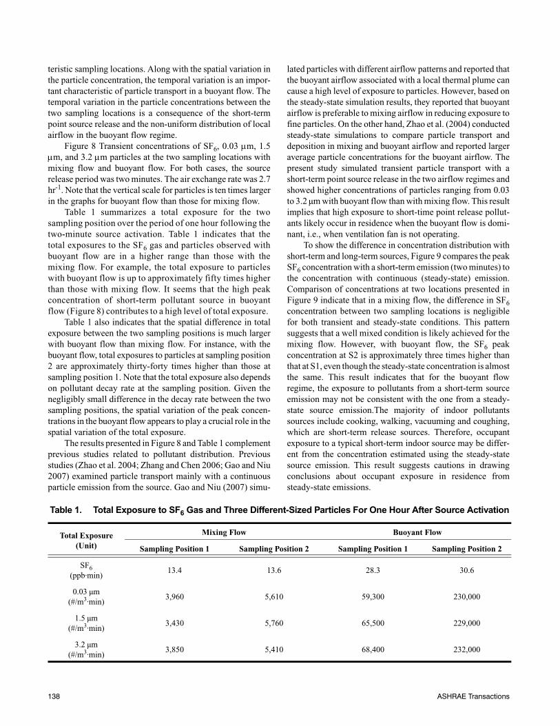
Table 1 summarizes a total exposure for the twosampling position over the period of one hour following thetwo-minute source activation. Table 1 indicates that thetotal exposures to the SF6 gas and particles observed withbuoyant flow are in a higher range than those with themixing flow. For example, the total exposure to particleswith buoyant flow is up to approximately fifty times higherthan those with mixing flow. It seems that the high peakconcentration of short-term pollutant source in buoyantflow (Figure 8) contributes to a high level of total exposure.

Table 1 also indicates that the spatial difference in totalexposure between the two sampling positions is much largerwith buoyant flow than mixing flow. For instance, with thebuoyant flow, total exposures to particles at sampling position2 are approximately thirty-forty times higher than those atsampling position 1. Note that the total exposure also dependson pollutant decay rate at the sampling position. Given thenegligibly small difference in the decay rate between the twosampling positions, the spatial variation of the peak concen-trations in the buoyant flow appears to play a crucial role in thespatial variation of the total exposure.

The results presented in Figure 8 and Table 1 complementprevious studies related to pollutant distribution. Previousstudies (Zhao et al. 2004; Zhang and Chen 2006; Gao and Niu2007) examined particle transport mainly with a continuousparticle emission from the source. Gao and Niu (2007) simu-

lated particles with different airflow patterns and reported thatthe buoyant airflow associated with a local thermal plume cancause a high level of exposure to particles. However, based onthe steady-state simulation results, they reported that buoyantairflow is preferable to mixing airflow in reducing exposure tofine particles. On the other hand, Zhao et al. (2004) conductedsteady-state simulations to compare particle transport anddeposition in mixing and buoyant airflow and reported largeraverage particle concentrations for the buoyant airflow. Thepresent study simulated transient particle transport with ashort-term point source release in the two airflow regimes andshowed higher concentrations of particles ranging from 0.03to 3.2 µm with buoyant flow than with mixing flow. This resultimplies that high exposure to short-time point release pollut-ants likely occur in residence when the buoyant flow is domi-nant, i.e., when ventilation fan is not operating.

To show the difference in concentration distribution withshort-term and long-term sources, Figure 9 compares the peakSF6 concentration with a short-term emission (two minutes) tothe concentration with continuous (steady-state) emission.Comparison of concentrations at two locations presented inFigure 9 indicate that in a mixing flow, the difference in SF6concentration between two sampling locations is negligiblefor both transient and steady-state conditions. This patternsuggests that a well mixed condition is likely achieved for themixing flow. However, with buoyant flow, the SF6 peakconcentration at S2 is approximately three times higher thanthat at S1, even though the steady-state concentration is almostthe same. This result indicates that for the buoyant flowregime, the exposure to pollutants from a short-term sourceemission may not be consistent with the one from a steady-state source emission.The majority of indoor pollutantssources include cooking, walking, vacuuming and coughing,which are short-term release sources. Therefore, occupantexposure to a typical short-term indoor source may be differ-ent from the concentration estimated using the steady-statesource emission. This result suggests cautions in drawingconclusions about occupant exposure in residence fromsteady-state emissions.

Table 1. Total Exposure to SF6 Gas and Three Different-Sized Particles For One Hour After Source Activation

Total Exposure(Unit)

Mixing Flow Buoyant Flow

Sampling Position 1 Sampling Position 2 Sampling Position 1 Sampling Position 2

SF6(ppb·min)

13.4 13.6 28.3 30.6

0.03 µm(#/m3·min)

3,960 5,610 59,300 230,000

1.5 µm(#/m3·min)

3,430 5,760 65,500 229,000

3.2 µm(#/m3·min)

3,850 5,410 68,400 232,000


Mechanically Ventilated Space vs. Naturally Ventilated Space

The room air exchange rate is generally higher in a roomwith a fan operating than a room in which only natural convec-tion airflow exists. This section of the present study examinespollutant transport in two typical residential rooms: a mechan-ically ventilated room with the mechanical fan ON and a natu-rally ventilated room with the fan OFF. The air exchange ratesused for a mechanically ventilated room and a naturally venti-lated room are 5 hr-1 and 0.5 hr-1, respectively.

Figure 10 shows the resulting SF6 and particle concentra-tions for the two analyzed rooms. The SF6 concentration in themechanically ventilated space is nearly uniform, implyingintensive mixing of the air in the space. However, spatial andtemporal variations in SF6 concentration and slower decay rate(after the peak) exist in the naturally ventilated room. This isdue to the non-uniform airflow distribution and low ventila-tion rate in the naturally ventilated room. The level of exposureto SF6 gas is higher in the naturally ventilated room comparedto the mechanically ventilated space. The particle concentra-tion data show a concentration pattern similar to SF6 results,including relatively uniform concentrations in the mechani-cally ventilated space, spatial and temporal variations inconcentrations and high exposure in the naturally ventilatedspace. However, the variation in particle concentration ishigher than that in SF6 concentration. The peak particleconcentration at S2 in the naturally ventilated space is up tothirty times higher than the one in the mechanically ventilatedspace, implying high potential of exposure to particles in the

naturally ventilated space. These results suggest that acuteexposure to transient pollutants can occur in a naturally venti-lated space where the pollutant distribution is not uniform andlocal zones of high pollutant concentration exist.

The results in Figure 9 and 10 indicate higher risk forexposure to particulate pollutants with buoyant flow.However, it should be pointed out that the gaseous andparticulate concentrations in a room depend on the sourceposition. In this study, the source was located close to thefloor and the effect of buoyant airflow on the pollutantconcentration at the sampling position seemed to be verylarge. Further investigations with different source locationsshould be conducted to articulate the effect of indoorairflow pattern on the transient pollutant concentrationpattern. Another limitation of this study is that thepresented results consider airflow and contaminant distri-bution in a space assuming clean supply air. With air recir-culation in air handling units, the recirculation rateinfluences the pollutant concentrations in the supply air.The effects of recirculation, including filtration and depo-sition of particles and reactions of gaseous pollutants inventilation systems, have an important role in occupantexposure. Therefore, in an overall analysis of contaminantdistribution in buildings, air recirculation should be takeninto account. When the recirculated pollutant concentra-tions are known, the results presented in this study can beused to recalculate pollutant dispersion considering pollut-ant concentration in supply air.

Figure 9 Comparison between SF6 peak (with intermittent injection) and steady-state (with continuous injection)concentrations at the two sampling locations with mixing flow and buoyant flow. For both cases, the air exchangerate was 2.7 hr–1.


CONCLUSION

In residential buildings, mechanical fans operate period-ically, and the present study simulated the indoor airflow asso-ciated with periodic fan usage. The transition period betweenmixing flow (fan ON) and buoyant flow (fan OFF) was foundto be approximately one minute, indicating that the airflow inresidence is primarily either mixing flow or buoyant flow.

A CFD model and experiments were used to simulate short-term point source pollutant release in the two airflow regimes.The results show that the peak concentrations of gaseous andparticulate pollutants can be much higher in a buoyant flow thanin a mixing flow. The variation in particle concentration washigher than that in gaseous concentration. These results implythat a high level of exposure to short-term point release pollutantslikely occurs in a residential room in which fan is not operating.The well-mixed assumption seems applicable in estimating thelevel of occupant exposure for mixing flow, but it is likely invalidto model exposure in a room with stratified flow. The comparisonof the peak concentrations due to a transient source and a steady-state concentration with a continuous source suggests cautions indrawing conclusions about occupant exposure to a short-termindoor pollutant release from the steady-state release concentra-tion, especially in a naturally ventilated space in which themechanical fan is off.

The study results clearly demonstrate that using the well-mixed and steady-state assumptions to estimate the occupantexposure may not always be appropriate for a naturally venti-lated residential space. Regarding the short-term exposure,future studies should assess the effect of source location on theexposure to pollutants.

ACKNOWLEDGMENTS

The research is partially supported by ASHRAE Grant-in-aid Fellowship and the National Science Foundation Inte-grative Graduate Education and Research Traineeship(IGERT) grant DCE-0549428, Indoor Environmental Scienceand Engineering, at The University of Texas at Austin. Theauthors are grateful for careful reviews of the manuscript byCatherine Mukai and Michael Waring.

REFERENCES

Abt, E., Suh, H.H., Catalano, P., and Koutrakis, P. 2000. Rel-ative contribution of outdoor and indoor particle sourcesto indoor concentrations. Environmental science & tech-nology 34 (17): 3579-3587.

Baughman, A.V., Gadgil, A.J., and Nazaroff, W.W. 1994.Mixing of a point-source pollutant by natural-convec-tion flow within a room. Indoor air 4 (2): 114-122.

Figure 10 Transient concentrations of SF6, 0.03 µm, 1.5 µm, and 3.2 µm particles at the two sampling locations for tworesidential rooms: mechanically ventilated (5hr–1) and naturally ventilated (0.5hr–1) rooms. Note that the verticalscale for particles if ten times larger in the graphs for buoyant flow than those for mixing flow.


Bouilly, J., Limam, K., Beghein, C., and Allard, F. 2005.Effect of ventilation strategies on particle decay ratesindoors: An experimental and modelling study. Atmo-spheric environment 39 (27): 4885-4892.

Chen, Q. 1995. Comparison of different k-? models forindoor air flow computations. Numerical heat transfer.Part B, Fundamentals, 28(3), 353-369.

Chen, Q. and Srebric, J. 2002. A procedure for verification,validation, and reporting of indoor environment CFDanalyses, Int. J. HVAC & R Res.,8, 201–216.

FLUENT, 2006. Fluent 6.2 User’s guide. Fluent Inc.,Lebanon, NH.

Ferro, A.R., Kopperud, R.J., and Hildemann, L.M. 2004.Source strengths for indoor human activities that resus-pend particulate matter. Environmental science & tech-nology 38 (6): 1759-1764.

Gao, N.P., and Niu, J.L. 2007. Modeling particle dispersionand deposition in indoor environments. Atmosphericenvironment 41 (18): 3862-3876.

He, CR., Morawska, L.D., Hitchins, J., and Gilbert, D. 2004.Contribution from indoor sources to particle number andmass concentrations in residential houses. Atmosphericenvironment 38 (21): 3405-3415.

He, G., Yang, X., and Srebric, J. 2005. Removal of contami-nants released from room surfaces by displacement andmixing ventilation: modeling and validation. Indoor air15 (5): 367-380.

Hinds W.C. 1999. Aerosol Technology. New York: Wiley. Huang, J.M., Chen, Q.Y., Ribot, B., and Rivoalen, H. 2004.

Modelling contaminant exposure in a single-familyhouse. Indoor and built environment 13 (1): 5-19.

Lai, A.C.K., and Nazaroff, WW. 2000. Modeling indoor par-ticle deposition from turbulent flow onto smooth sur-faces. Journal of aerosol science 31 (4): 463-476.

Li, Y., Leung, G.M., Tang, J.W., Yang, X., Chao, C.Y.H.,Lin, J.Z., Lu, J.W., Nielsen, P.V., Niu, J., Qian, H.,Sleigh, A.C., Su, H.J.J., Sundell, J., Wong, T.W., andYuen, P.L. 2007. Role of ventilation in airborne trans-mission of infectious agents in the built environment -a multidisciplinary systematic review. Indoor air17(1): 2-18.

Lin, Z., Chow, T.T., Fong, K.F., Tsang, C.F., and Wang, Q.W.2005. Comparison of performances of displacement andmixing ventilations. Part II: indoor air quality. Revueinternationale du froid, 28(2): 288-305.

Murakami, S., Kato, S., Zeng, J. 1997. Flow and temperaturefields around the human body with various room air dis-tribution, CFD study on computational thermal manikin– Part I. ASHRAE Transactions 103:3-15

Nazaroff, WW. 2004. Indoor particle dynamics. Indoor air14: 175-183.

Nemmar, A., Hoet, P.H.M., Vanquickenborne, B., Dinsdale,D., Thomeer, M., Hoylaerts, M.F., Vanbilloen, H.,Mortelmans, L., and Nemery, B. 2002. Passage of

inhaled particles into the blood circulation in humans.Circulation 105 (4): 411-414.

Novoselac, A., and Srebic, J. 2002. A critical review on theperformance and design of combined cooled ceiling anddisplacement ventilation systems. Energy and buildings34 (5): 497-509.

Penttinen, P., Timonen, K.L., Tiittanen, P., Mirme, A., Ruus-kanen, J., and Pekkanen, J. 2001. Ultrafine particles inurban air and respiratory health among adult asthmatics.The European respiratory journal 17 (3): 428-435.

Posner, J.D., Buchanan, C.R., and Dunn-Rankin, D. 2003.Measurement and prediction of indoor air flow in amodel room. Energy and buildings 35 (5): 515-526.

Riley, W.J., McKone, K.E., Lai, A.C.K., and Nazaroff, W.W.2002. Indoor particulate matter of outdoor origin:Importance of size-dependent removal mechanisms.Environmental science & technology 36 (2): 200-207.

Sørensen, D.N., and Neilsen, P.V. 2003. Quality control ofcomputational fluid dynamics in indoor environments.Indoor air 13 (1): 2-17.

Topp, C., Nielsen, P.V. and Sørensen, D.N. 2002. Applica-tion of Computer Simulated Persons in Indoor Envi-ronmental Modeling. ASHRAE Transactions, 108(2), p. 1084-1089.

Ward, M., Siegel, J.A., and Corsi, R.L. 2005. The effective-ness of stand alone air cleaners for shelter-in-place.Indoor air 15 (2): 127-134.

Zhang, Z., and Chen, Q. 2006. Experimental measurementsand numerical simulations of particle transport and dis-tribution in ventilated rooms. Atmospheric environment40 (18): 3396-3408.

Zhao, B., Li, X.T., and Zhang, Z. 2004. Numerical study ofparticle deposition in two differently ventilated rooms.Indoor and built environment 13 (6): 443-451.

DISCUSSION

H. Ezzat Khalifa, Professor, Syracuse University, Syra-cuse, NY: There was a paper by Sideroff et al. in TransactionsSession 2 yesterday in which a very detailed representation ofthe manikin and its microenvironment was included in severalCFD simulations with k-ε, Vzf, and LES models. The resultswere compared with experimental data obtained by ProfessorsNielsen and Katz. Sideroff showed little advantage of LESover k-ε with each wall treatment. He found the inclusion ofradiation in CFD is far more important.Donghyun Rim: We agree with Professor Khalifa's comment,and that is the reason we used k-ε turbulence model in our simu-lations. Also, in our CFD models we took into account effectsof radiation by calculating convective and radiative portions ofheat fluxes at surfaces based on experimental results. By usingonly the convective portion of the total heat flux for Neumannboundary conditions, we secured accuracy of thermal boundaryconditions in our CFD and particle tracking models.Paul Lebbin, Mechanical Engineer, J.L. Richards & Asso-ciates, North Bay, ON, Canada: Very interesting results


between measured and predicted CFD results. I would haveliked a detailed description of the measurement equipment tosee how the particles are released/measured. As you know, thisis criteria in CFD verification.Donghyun Rim: In our validation experiments, we used latexmonodispersed particles with a density of 1.05 g/cm3. Sepa-rate experiments were conducted for 0.03, 1.5, and 3.2 μmparticles. The particles were seeded with a constant rate at thesource position using the Collison Nebulizer. The particle

injection created a several-order higher particle concentrationin the space than the initial (background) concentration. Thisway, we eliminated inaccuracy in measurement caused by thebackground concentration. We monitored spatial and tempo-ral distribution of 0.03 μm particles using condensation parti-cle counters (CPC), and for 1.5 and 3.2 μm particles we usedoptical particle counters (OPC). All of the instruments used inour study were calibrated before the measurements.


sl-08-013 transient simulation of airflow and pollutant ... · ashrae transactions 131 pollutants...

Documents