Computational Statistics (2008) 23:429–442DOI 10.1007/s00180-007-0083-7

ORIGINAL PAPER

Goodness-of-fit tests based on a robust measureof skewness

Guy Brys · Mia Hubert · Anja Struyf

Accepted: 20 June 2007 / Published online: 23 August 2007© Springer-Verlag 2007

Abstract In this paper we propose several goodness-of-fit tests based on robustmeasures of skewness and tail weight. They can be seen as generalisations of theJarque–Bera test (Bera and Jarque in Econ Lett 7:313–318, 1981) based on the classicalskewness and kurtosis, and as an alternative to the approach of Moors et al. (Stat Neerl50:417–430, 1996) using quantiles. The power values and the robustness propertiesof the different tests are investigated by means of simulations and applications onreal data. We conclude that MC-LR, one of our proposed tests, shows the best overallpower and that it is moderately influenced by outlying values.

Keywords Tail weight · Robustness · Jarque–Bera test

1 Introduction

The third and fourth moments of a distribution are called the skewness and kurtosis.For any distribution F with finite central moments µk up to k = 3, the skewness is

G. BrysFPS Economy, Directorate-General Statistics Belgium, Leuvenseweg 44, 1000 Brussels, Belgiume-mail: Guy.Brys@economie.fgov.be

M. Hubert (B)Department of Mathematics and UCS, Katholieke Universiteit Leuven (KULeuven),Celestijnenlaan 300 B, 3001 Leuven, Belgiume-mail: Mia.Hubert@wis.kuleuven.be

A. StruyfDepartment of Mathematics and Computer Sciences, University of Antwerp (UA),Middelheimlaan 1, 2020 Antwerp, Belgiume-mail: Anja.Struyf@ua.ac.be

123

430 G. Brys et al.

defined as

γ1(F) = µ3(F)

µ2(F)3/2 .

Skewness describes the asymmetry of a distribution. A symmetric distribution haszero skewness, an asymmetric distribution with the largest tail to the right has positiveskewness, and a distribution with a longer left tail has negative skewness.

For any distribution F with finite central moments µk up to k = 4, the kurtosis isdefined as

γ2(F) = µ4(F)

µ2(F)2 .

There is no agreement on what it really measures. Strictly speaking, kurtosis measuresboth peakedness and tail heaviness of a distribution relative to that of the normal dis-tribution. Consequently, its use is restricted to symmetric distributions. Finite-sampleversions of γ1 and γ2 will be denoted by b1 and b2.

The classical skewness and kurtosis coefficient have some common disadvantages.They both have a zero breakdown value and an unbounded influence function, and sothey are very sensitive to outlying values. One single outlier can make the estimatebecome very large or small, making it hard to interpret. Another disadvantage is thatthey are only defined on distributions having finite moments.

In Sect. 2 we propose several measures of skewness and of left and right tail weightfor univariate continuous distributions. Their interpretation is clear and they are robustagainst outlying values. Contrary to the kurtosis coefficient, the tail weight measurescan be applied to symmetric as well as asymmetric distributions. In Sect. 3 we introducesome robust goodness-of-fit tests. Sections 4 and 5 include simulation results whileSect. 6 applies the tests on real data. Finally, Sect. 7 concludes.

2 Robust measures of skewness and tail weight

Assume we have independently sampled n observations Xn = {x1, x2, . . . , xn} from acontinuous univariate distribution F . We will consider the medcouple (MC), a robustskewness measure, proposed in Brys et al. (2003) and extensively discussed in Bryset al. (2004a). It is defined as

MC(F) = medx1<m F <x2

h(x1, x2)

with x1 and x2 sampled from F , m F = F−1(0.5) and the kernel function h given by

h(xi , x j ) = (x j − m F ) − (m F − xi )

x j − xi.

This estimator has a breakdown value of 25% and a bounded influence function.Furthermore, we consider the left medcouple (LMC) and right medcouple (RMC),

respectively, the left and right tail weight measure, as defined in Brys et al. (2006). Toconstruct these measures we have applied the medcouple to, respectively, the left and

123

Goodness-of-fit tests based on a robust measure of skewness 431

right half of the samples:

LMC(F) = −MC(x < m F ) and RMC(F) = MC(x > m F ),

yielding a breakdown value of 12.5%.Finite sample versions will be denoted by MCn , LMCn and RMCn . These measures

can be computed at any distribution, even when finite moments do not exist. Theircomputation can be performed in O(n log n) time due to the fast algorithm describedin Brys et al. (2004a). They satisfy all natural requirements of skewness or tail weightmeasures including location and scale invariance. More details can be found in thecited references.

3 Description of the tests

In this section we discuss goodness-of-fit tests for the following null and alternativehypothesis:

{H0 : The sample is drawn from a distribution FH1 : The sample is not drawn from a distribution F.

In this paper we will investigate the performance of the tests at F taken to be theχ2

2 distribution, the Student t3 distribution and the Tukey’s class of gh-distributions(Hoaglin et al. 1985). When a random variable Z is standard gaussian distributed, then

Yg,h =⎧⎨⎩

(egZ −1)g e

h Z22 g �= 0

Zeh Z2

2 g = 0

is said to follow a gh-distribution Gg,h with parameters g ∈ R and h ≥ 0. Theparameter g controls the skewness of the distribution, whereas h effects the tail weight.

Bera and Jarque (1981) proposed a normality test using the classical skewnessand kurtosis coefficient. As been stated in Moors et al. (1996), under the normalityassumption (γ1 = 0 and γ2 = 3) we can write:

√n

(b1b2

)→D N2

((03

),

(6 00 24

))

which leads to the Jarque–Bera test statistic:

T = n

(b2

1

6+ (b2 − 3)2

24

)≈ χ2

2 .

This test can be viewed as a special case of the following generalization. Let w =(w1, w2, . . . , wk)

t be estimators of ω = (ω1, ω2, . . . , ωk)t , such that

√n

(w1 . . . wk

)t →D Nk (ω,�k)

123

432 G. Brys et al.

Table 1 Asymptotic mean ω and covariance matrix �k of the (joint) distribution of several measures ofskewness and tail weight, used in the JB test, the MOORS test and the MC-LR test

ω(JB) �k (JB) ω(MOORS) �k (MOORS) ω(MC-LR) �k (MC-LR)

G0,0

(03

) (6 00 24

) (0

1.23

) (1.84 0

0 3.14

) ⎛⎝ 0

0.1990.199

⎞⎠

⎛⎝ 1.25 0.323 −0.323

0.323 2.62 −0.0123−0.323 −0.0123 2.62

⎞⎠

χ22

(29

) (72 720720 8.06e(3)

) (0.2621.31

) (1.78 −0.152

−0.152 5.09

) ⎛⎝0.338−0.1090.333

⎞⎠

⎛⎝ 1.27 0.360 −0.310

0.360 2.75 −1.87e(−5)

−0.310 −1.87e(−5) 2.54

⎞⎠

t3

(−−

) (− −− −

) (0

1.40

) (1.87 0

0 4.62

) ⎛⎝ 0

0.2970.297

⎞⎠

⎛⎝ 1.36 0.221 −0.221

0.221 2.58 −0.0231−0.221 −0.0231 2.58

⎞⎠

Note that 1e(3) stands for 1,000

then, under H0, the generalized test statistic T

T = n(w − ω)t�−1k (w − ω) ≈ χ2

k .

We can thus easily construct new goodness-of-fit tests, analogous to Brys et al.(2004b). Taking k = 2, w1 = b1 and w2 = b2 leads to the generalized Jarque–Beratest (JB) with ω1 = γ1 and ω2 = γ2. A test based on the medcouple (MC) given inBrys et al. (2004a) has k = 1 and w1 = MC. Secondly, Brys et al. (2006) propose touse the test of LMC or RMC with k = 1 and w1 = LMC or w1 = RMC. Combiningthe skewness and, respectively, the left and right tail weight of a distribution leadsto MC-L and MC-R with k = 2, w1 = MC, and, respectively, w2 = LMC andw2 = RMC. Next, we can define a test based on the left and right medcouple (LR)with k = 2, w1 = LMC and w2 = RMC. Finally, we propose a goodness-of-fit testMC-LR where k = 3, w1 = MC, w2 = LMC and w3 = RMC.

We will also include a test proposed in Moors et al. (1996). This test (MOORS) fits in

the framework of the above generalization by usingw1 = F−1(0.75)+F−1(0.25)−2F−1(0.5)

F−1(0.75)−F−1(0.25)

as a robust measure of skewness and w2 = F−1(0.875)−F−1(0.625)+F−1(0.375)−F−1(0.125)

F−1(0.75)−F−1(0.25)

as a robust measure of kurtosis. By using only quantiles of the data this test is resistantto 12.5% outliers in the data. This is the same as for all tests based on LMC and/orRMC.

Table 1 shows the values of ω and �k for several distributions F for the generalizedJarque–Bera test, the MOORS test and the MC-LR test. By using the latter it is possibleto write down ω and �k for the other goodness-of-fit tests based on MC. Table 1 isderived from the influence function of the estimators, as described in Brys et al. (2004a)and in Brys et al. (2006).

4 Simulation study at uncontaminated distributions

We investigate the seven proposed tests by generating m = 1,000 samples of sizen = 100 and n = 1,000 from a wide range of distributions. Note that in all Figuresin this Section and in Sect. 5 the upper panel represents the results for n = 100 and

123

Goodness-of-fit tests based on a robust measure of skewness 433

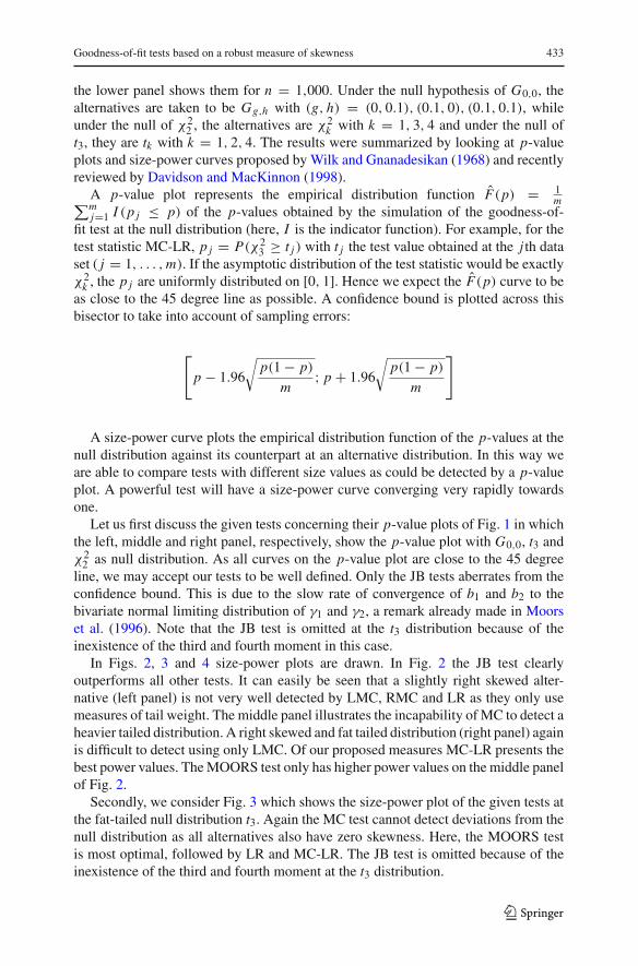
the lower panel shows them for n = 1,000. Under the null hypothesis of G0,0, thealternatives are taken to be Gg,h with (g, h) = (0, 0.1), (0.1, 0), (0.1, 0.1), whileunder the null of χ2

2 , the alternatives are χ2k with k = 1, 3, 4 and under the null of

t3, they are tk with k = 1, 2, 4. The results were summarized by looking at p-valueplots and size-power curves proposed by Wilk and Gnanadesikan (1968) and recentlyreviewed by Davidson and MacKinnon (1998).

A p-value plot represents the empirical distribution function F̂(p) = 1m∑m

j=1 I (p j ≤ p) of the p-values obtained by the simulation of the goodness-of-fit test at the null distribution (here, I is the indicator function). For example, for thetest statistic MC-LR, p j = P(χ2

3 ≥ t j ) with t j the test value obtained at the j th dataset ( j = 1, . . . , m). If the asymptotic distribution of the test statistic would be exactlyχ2

k , the p j are uniformly distributed on [0, 1]. Hence we expect the F̂(p) curve to beas close to the 45 degree line as possible. A confidence bound is plotted across thisbisector to take into account of sampling errors:

[p − 1.96

√p(1 − p)

m; p + 1.96

√p(1 − p)

m

]

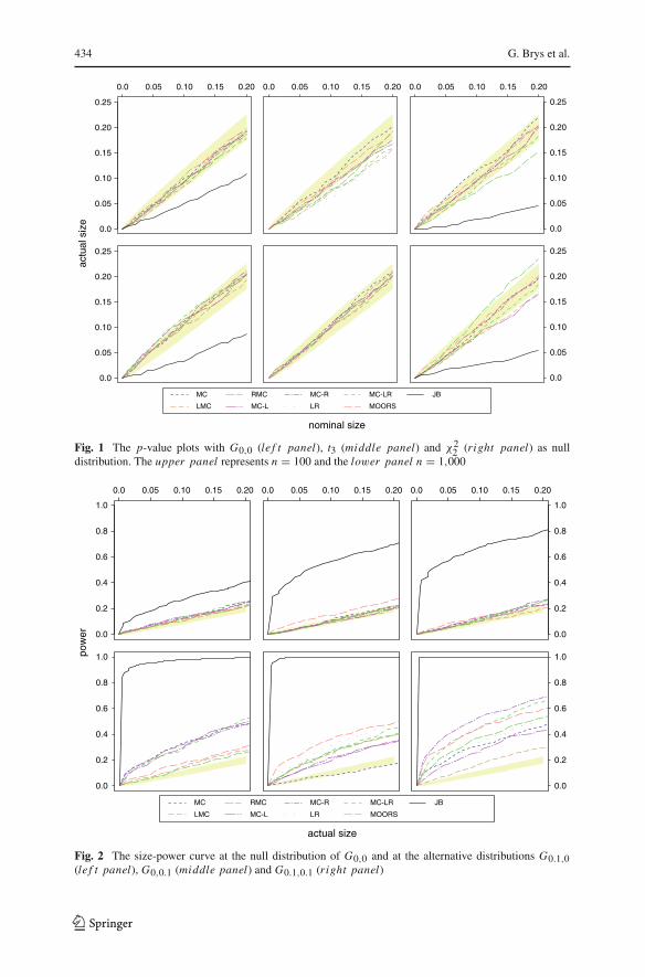
A size-power curve plots the empirical distribution function of the p-values at thenull distribution against its counterpart at an alternative distribution. In this way weare able to compare tests with different size values as could be detected by a p-valueplot. A powerful test will have a size-power curve converging very rapidly towardsone.

Let us first discuss the given tests concerning their p-value plots of Fig. 1 in whichthe left, middle and right panel, respectively, show the p-value plot with G0,0, t3 andχ2

2 as null distribution. As all curves on the p-value plot are close to the 45 degreeline, we may accept our tests to be well defined. Only the JB tests aberrates from theconfidence bound. This is due to the slow rate of convergence of b1 and b2 to thebivariate normal limiting distribution of γ1 and γ2, a remark already made in Moorset al. (1996). Note that the JB test is omitted at the t3 distribution because of theinexistence of the third and fourth moment in this case.

In Figs. 2, 3 and 4 size-power plots are drawn. In Fig. 2 the JB test clearlyoutperforms all other tests. It can easily be seen that a slightly right skewed alter-native (left panel) is not very well detected by LMC, RMC and LR as they only usemeasures of tail weight. The middle panel illustrates the incapability of MC to detect aheavier tailed distribution. A right skewed and fat tailed distribution (right panel) againis difficult to detect using only LMC. Of our proposed measures MC-LR presents thebest power values. The MOORS test only has higher power values on the middle panelof Fig. 2.

Secondly, we consider Fig. 3 which shows the size-power plot of the given tests atthe fat-tailed null distribution t3. Again the MC test cannot detect deviations from thenull distribution as all alternatives also have zero skewness. Here, the MOORS testis most optimal, followed by LR and MC-LR. The JB test is omitted because of theinexistence of the third and fourth moment at the t3 distribution.

123

434 G. Brys et al.

nominal size

ezis lautca0.0 0.05 0.10 0.15 0.20

0.0

0.05

0.10

0.15

0.20

0.25

0.0 0.05 0.10 0.15 0.20 0.0 0.05 0.10 0.15 0.20

0.0

0.05

0.10

0.15

0.20

0.25

0.0

0.05

0.10

0.15

0.20

0.25

0.0

0.05

0.10

0.15

0.20

0.25

MC

LMC

RMC

MC-L

MC-R

LR

MC-LR

MOORS

JB

Fig. 1 The p-value plots with G0,0 (le f t panel), t3 (middle panel) and χ22 (right panel) as null

distribution. The upper panel represents n = 100 and the lower panel n = 1,000

actual size

rewop

0.0 0.05 0.10 0.15 0.20

0.0

0.2

0.4

0.6

0.8

1.0

0.0 0.05 0.10 0.15 0.20 0.0 0.05 0.10 0.15 0.20

0.0

0.2

0.4

0.6

0.8

1.0

0.0

0.2

0.4

0.6

0.8

1.0

0.0

0.2

0.4

0.6

0.8

1.0

MC

LMC

RMC

MC-L

MC-R

LR

MC-LR

MOORS

JB

Fig. 2 The size-power curve at the null distribution of G0,0 and at the alternative distributions G0.1,0(le f t panel), G0,0.1 (middle panel) and G0.1,0.1 (right panel)

123

Goodness-of-fit tests based on a robust measure of skewness 435

actual size

pow

er0.0 0.05 0.10 0.15 0.20

0.0

0.2

0.4

0.6

0.8

1.0

0.0 0.05 0.10 0.15 0.20 0.0 0.05 0.10 0.15 0.20

0.0

0.2

0.4

0.6

0.8

1.0

0.0

0.2

0.4

0.6

0.8

1.0

0.0

0.2

0.4

0.6

0.8

1.0

MC

LMC

RMC

MC-L

MC-R

LR

MC-LR MOORS

Fig. 3 The size-power curve at the null distribution of t3 and at the alternative distributions t1 (le f t panel),t2 (middle panel) and t4 (right panel)

actual size

rewop

0.0 0.05 0.10 0.15 0.20

0.0

0.2

0.4

0.6

0.8

1.0

0.0 0.05 0.10 0.15 0.20 0.0 0.05 0.10 0.15 0.20

0.0

0.2

0.4

0.6

0.8

1.0

0.0

0.2

0.4

0.6

0.8

1.0

0.0

0.2

0.4

0.6

0.8

1.0

MC

LMC

RMC

MC-L

MC-R

LR

MC-LR

MOORS

JB

Fig. 4 The size-power curve at the null distribution of χ22 and at the alternative distributions χ2

1(le f t panel), χ2

3 (middle panel) and χ24 (right panel)

123

436 G. Brys et al.

In case χ22 is taken as the null distribution, we obtain in Fig. 4 the resulting size-

power plot. Here, the MC-LR test and the MC-R test appear to be the best one, althoughat n = 100 they are sometimes outperformed by the JB test.

5 Simulation study at contaminated distributions

In this section we want to compare the proposed tests with respect to their robust-ness. To this end, we generated here contaminated m = 1,000 samples of sizen = 100 and n = 1,000 of a distribution F by taking a sample of size n(1 − ε)

of that distribution F and adding a contaminated sample of size nε. The lattercan be N (F−1(0.5) + 2 ∗ F−1(0.999) − F−1(0.001), 0.1) (right contamination,RC), N (F−1(0.5), F−1(0.999) − F−1(0.001)) (symmetric contamination, SC),N (F−1(0.5) + 2 ∗ F−1(0.001) − F−1(0.999), 0.1) (left contamination, LC) orN (F−1(0.5), F−1(0.51) − F−1(0.49)) (central contamination, CC). Here we havetaken ε = 0.01 and ε = 0.02.

We will restrict ourselves to two tests, namely the MOORS test and MC-LR. Theother proposed robust alternatives are omitted due to their lower power values. Fur-thermore, the JB goodness-of-fit test is absolutely not able to handle outlying values.In our simulations we noticed that the JB test is highly sensitive to right, symmetricand left contamination, as they have a large impact on the third and/or fourth mo-ment of the distribution. The JB test was only able to cope reasonably with centralcontamination which does not change the skewness and did not have a too large impacton the kurtosis.

From Figs. 5 and 6 it is straightforward to see that the MOORS test and the MC-LRtest behave fairly correct in presence of outliers. When ε increases the MC-LR testdeviates more strongly than the MOORS test from the confidence bound, especiallyat n = 1,000 (lower panel of Fig. 6). Nevertheless, compared to the generalizedJarque–Bera test, the MC-LR test is extremely better able to handle outlying values.

6 Applications

In this section we analyze four data sets which illustrate the robustness of the MOORSand the MC-LR test compared to the JB test.

The first data set comes from the Associated Examining Board in Guilford(Cresswell 1990) and contains a sample of 1,000 scores of students on the writingof a paper. From the normal QQ-plot of Fig. 7a and the boxplot in Fig. 7b the as-sumption of normality seems appropriate. Only four minor outliers are visible on theboxplot. In Table 2 the non-robustness of the JB test is illustrated. Normality is rejectedat the 5% significance level when the outliers from the boxplot are included, but isaccepted when they are excluded. On the contrary, the MOORS test and our proposedMC-LR test is based on the majority of the data and so they behave the same in bothsituations. As could be expected, they all detect normality in this data set.

The stars data set (Rousseeuw and Leroy 1987) contains the light intensity andthe surface temperature of 47 stars in the direction of Cygnus. A scatter plot of thedata and the robust LTS regression line (Rousseeuw 1984) are shown in Fig. 8a.

123

Goodness-of-fit tests based on a robust measure of skewness 437

nominal size

ezis lautca0.0 0.05 0.10 0.15 0.20

0.0

0.05

0.10

0.15

0.20

0.25

0.0 0.05 0.10 0.15 0.20 0.0 0.05 0.10 0.15 0.20

0.0

0.05

0.10

0.15

0.20

0.25

0.0

0.05

0.10

0.15

0.20

0.25

0.0

0.05

0.10

0.15

0.20

0.25

MOORS, RC(1%)

MOORS, SC(1%)

MOORS, LC(1%)

MOORS, CC(1%)

MC-LR, RC(1%)

MC-LR, SC(1%)

MC-LR, LC(1%)

MC-LR, CC(1%)

Fig. 5 The p-value plot at the null distribution of G0,0 (le f t panel), of t3 (middle panel), and of χ22

(right panel), contaminated case with ε = 0.01

nominal size

ezis lautca

0.0 0.05 0.10 0.15 0.20

0.0

0.05

0.10

0.15

0.20

0.25

0.0 0.05 0.10 0.15 0.20 0.0 0.05 0.10 0.15 0.20

0.0

0.05

0.10

0.15

0.20

0.25

0.0

0.05

0.10

0.15

0.20

0.25

0.0

0.05

0.10

0.15

0.20

0.25

MOORS, RC(2%)

MOORS, SC(2%)

MOORS, LC(2%)

MOORS, CC(2%)

MC-LR, RC(2%)

MC-LR, SC(2%)

MC-LR, LC(2%)

MC-LR, CC(2%)

Fig. 6 The p-value plot at the null distribution of G0,0 (le f t panel), of t3 (middle panel), and of χ22

(right panel), contaminated case with ε = 0.02

123

438 G. Brys et al.

quantiles

atad

-3 -2 -1 0 1 2 3

3-2-

1-0

12

3-2-

1-0

12

a

b

Fig. 7 The Guilford data: a normal QQ-plot, b boxplot

Table 2 Significance of thegoodness-of-fit tests, withoutliers included or excluded

JB MOORS MC-LR

Guilford, outliers included 0.039 0.496 0.975

Guilford, outliers excluded 0.087 0.497 0.995

Stars, outliers included 0.000 0.867 0.290

Stars, outliers excluded 0.301 0.320 0.377

Baseball, outliers included 0.000 0.261 0.104

Baseball, outliers excluded 0.919 0.717 0.213

Procter, outliers included – 0.573 0.652

Procter, outliers excluded – 0.491 0.606

123

Goodness-of-fit tests based on a robust measure of skewness 439

light intensity

erutarepme t ecafrus

3.6 3.8 4.0 4.2 4.4 4.6

0.45.4

0.55. 5

0.6

LS

LTS

quantiles

atad

-2 -1 0 1 2

1-0

12

31-

01

23

a b

c

Fig. 8 The Stars data: a scatter plot with LTS regression line, b normal QQ-plot of the residuals, c boxplotof the residuals

In regression, it is important to check normality of the residuals. Figure 8b and ccontain the normal QQ-plot and the boxplot of the LTS residuals, from which fiveclear outliers are visible. It is known that the four largest residuals correspond withgiant stars. The sixth observation that seems to deviate from the linear trend in thenormal quantile plot is rather a borderline case with a standardized LTS residual of3.47. Table 2 shows again that the JB test leads to very different conclusions whetheror not these five outliers are included in the data. Both MOORS and MC-LR arenot highly influenced by these outliers and confirm the normality assumption that issatisfied by the large majority of the data. It should be emphasized that the JB test doesnot come to incorrect conclusions as the full data set is indeed not sampled from anormal distribution. Applying the robust tests as well gives us additional information.The rejection by JB is not due to an overall deviation from the normal distribution, butit is caused by a few outliers which clearly come from a different distribution.

The baseball data (Reichler 1991) consists of 162 major league baseball playerswho achieved true free agency. This means that the player could sell his services tothe highest bidding team. A player is expected to handle in two possible directions. Orhe plays badly in the year of his free agency, because he is unhappy with his currentteam and he will play much better in the next year. Or he pushes his performance inhis free agency year in order to get to a better team, but then he will play less well thenext year. Here, we wanted to test whether the batting average (hits per at bat) at thefree agency year and at the next year is bivariate normally distributed. Therefore wecalculated the robust distances given by

(x − µ̂)t �̂−1(x − µ̂)

123

440 G. Brys et al.

quantiles

atad

0 1 2 3 4 5

05

0151

0252

03

Fig. 9 The Baseball data: χ22 based QQ-plot of the robust distances

in which µ̂ and �̂ are the Minimum Covariance Estimator (MCD) estimates of locationand scatter (Rousseeuw 1984). If the data follow a bivariate normal distribution, theserobust distances are approximately χ2

2 distributed. On the χ22 based QQ-plot of Fig. 9

we notice two prominent outliers. With these outliers included, the generalized Jarque–Bera test rejects the null hypothesis, but the robust tests accept that the majority of thedistances are χ2

2 distributed. When excluding these two extreme values, both the JBand the robust tests accept the null hypothesis.

From Datastream we collected the daily logaritmic returns of the Procter & Gamblestock from January 2000 to December 2003, leading to a univariate data set consistingof 1004 values. From the t3 based QQ-plot of Fig. 10, we could believe these data tobe likewise distributed, apart from one very abnormal observation. This observationis noted on 7 March 2000, the day that Procter & Gamble has lost 40 billion of USDollars due to a profit warning. Indeed, both the MOORS and the MC-LR test donot reject the null hypothesis, which is probably due to the majority of points whichfollow closely the imaginary line on the QQ-plot. Excluding the extreme value did notchange the results. Here, we see an additional advantage of the robust tests: as they donot depend on moments of the data, they can also be used to test the goodness-of-fit ofdistributions such as the t3. On the contrary, the generalized JB test cannot be appliedhere.

7 Conclusion

In this paper we discussed several goodness-of-fit tests in terms of robustness. Thecommonly used Jarque–Bera test of normality was extended to become a goodness-of-fit test. Main advantage of the generalized Jarque–Bera test is that its power values arereasonably high. But, by means of p-value plots and size-power curves we noted that

123

Goodness-of-fit tests based on a robust measure of skewness 441

quantiles

atad

-5 0 5

51-01-

5-0

5

Fig. 10 The Procter & Gamble data: t3 based QQ-plot

this test often fails to lead to a correct actual size, due to the slow rate of convergencetowards the limiting distribution. Moreover, the test cannot be performed at distribu-tions without finite moments, and as it is based on moments of the data it is stronglyinfluenced by the presence of outlying values.

Therefore Moors et al. (1996) proposed to replace the classical skewness andkurtosis coefficient by robust alternatives, leading to the MOORS test. We conducteda similar approach by using the measures proposed in Brys et al. (2004a), (2006).Combining the medcouple (MC), a robust skewness measure, with left and right tailweight measures (LMC and RMC), we constructed the MC-LR test, which came out tobe the best of our proposed robust goodness-of-fit tests. Indeed, it appeared to be welldefined at the null distribution and it also appeared to be quite powerful. Comparedto the MOORS test the MC-LR test has often higher power values, and comparablesensitivity towards outliers.

In practice, we recommend to perform both the JB test and the robust MC-LR test.If they give contradictory answers, this can either be due to the failure of the JB testin the presence of outliers, or due to the conservative behaviour of the MC-LR test. Inthat case, a further investigation of the data is required.

References

Bera A, Jarque C (1981) Efficient tests for normality, heteroskedasticity and serial independence ofregression residuals: Monte Carlo evidence. Econ Lett 7:313–318

Brys G, Hubert M, Struyf A (2003) A comparison of some new measures of skewness. In: Developmentsin Robust Statistics, ICORS 2001. pp 98–113

Brys G, Hubert M, Struyf A (2004a) A robust measure of skewness. J Comput Graph Stat 13:996–1017Brys G, Hubert M, Struyf A (2004b) A robustification of the Jarque–Bera test of normality. In: COMPSTAT

2004 Proceedings, pp 753–760

123

442 G. Brys et al.

Brys G, Hubert M, Struyf A (2006) Robust measures of tail weight. Comput Stat Data Anal 50:733–759Cresswell MJ (1990) Gendar effects in GCSE, some initial analyses. Research Report. Associated

Examining Board, Guilford 517Davidson R, MacKinnon JG (1998) Graphical methods for investigating the size and power of test statistics.

Manchester Sch 66:1–26Hoaglin DC, Mosteller F, Tukey JW (1985) Exploring data tables, trends and shapes. Wiley, LondonMoors JJA, Wagemakers RTA, Coenen VMJ, Heuts RMJ, Janssens MJBT (1996) Characterizing systems

of distributions by quantile measures. Stat Neerl 50:417–430Reichler JL (1991) The baseball encyclopedia. Macmillan, New YorkRousseeuw PJ (1984) Least median of squares regression. J Am Stat Assoc 79:871–881Rousseeuw PJ, Leroy AM (1987) Robust regression and outlier detection. Wiley, LondonSmirnov NV (1948) Table for estimating the goodness of fit of empirical distributions. Ann Math Stat

19:279–281Wilk MB, Gnanadesikan R (1968) Probability plotting methods for the analysis of data. Biometrika

33(1):1–17

123