Single Phase Convective Heat Transfer with

Nanofluids: An Experimental Approach

Ehsan Bitaraf Haghighi

Division of Applied Thermodynamics and RefrigerationDepartment of Energy TechnologyRoyal Institute of Technology

Contents

• Introduction

• Project Foundation and Backdrop

• Aim of the Study and Methodology

• Experimental Approach

• Theoretical and Empirical Formulas

• Summary of Results and Discussion

• Conclusion and Future Work

2

My Daily Life!

3

What is a Nanofluid?

4

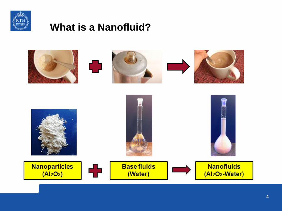
What is a Nanofluid?

Dilute dispersions of nanoparticles (NPs) with usually loading less than 5 vol%

in conventional heat transfer fluids or base fluids (BFs) are nanofluids (NFs)

(like metals, metal oxides, carbides, carbon nanotubes etc.)

(like water, ethylene glycol/water, oils etc.)

5

Why Nanofluids are Interesting?

6

490429

401

317

368.4 0.606 0.250 0.145

0

100

200

300

400

500

k (

W/m

K)

Material

Nanofluids in the Literature

499527

396

182

13090

6735 23 14 3 1 0 1 0 1 2 0 0 0 2

0

100

200

300

400

500

600

Re

co

rds

Year

Source: Engineering Village

Articles with term

“nanofluid” in their titles

7

Chip Heat Flux Trends & Prediction

Source: National Electronics Manufacturing Initiative (NEMI), 2000

Accommodate

q = 120 W/cm2

at ΔT = 50 K

Requires

h = 24 000 W/m2K

8

Attainable Heat Transfer Coefficient

Source: Lasance, C., Technical Data column, Electronics Cooling, January 1997

9

Project Foundation and Backdrop

• NanoHex (Enhanced Nanofluid Heat Exchange)

• A consortium of twelve leading European companies and

research centres

• Granted €8.3 million by the Seventh Framework

Programme (FP7)

• September 2009 - April 2013

• Aim: improve heat management in existing industries,

particularly data centres and power electronics

• The main goal: to develop a formulation and a production

pilot–line for a promising nanofluid as a coolant

10

NanoHex: 12 Work Packages (WP) and Main Role of KTH

11

Aim of the Study

• Answer to this question “if NFs can replace common

BFs?”

• Have a critical approach to previous literature

• Suggest rather rapid experimental and analytical

screening methods for evaluating the cooling performance

of NFs

• Find a simple, inexpensive and standardized method to

estimate the shelf stability of NFs

12

Methodology

Investigate thermophysical and transport properties of NFs

Theoretical analysis

Investigate shelf stability of NFs

Thermal conductivity

Viscosity

Density

Specific Heat

Heat transfer

coefficient Measurement

Formula

Measurement

screening setup

closed loop

13

Methodology

Can we simplify this?

14

Experimental Approach

• Thermal Conductivity

• Viscosity

• Convective Heat Transfer

• Screening setup

• Convective closed–loop

• Shelf Stability

• Material Characterisation

15

Thermal Conductivity

16

Viscosity

17

Screening Setup Test Section (din=0.5 mm, L=30 cm)

ℎ𝑥 =𝑞"

𝑇𝑠−𝑖𝑛,𝑥 − 𝑇𝑓,𝑥

𝑇𝑓,𝑥 = 𝑇𝑖𝑛𝑙𝑒𝑡 +𝑞"𝜋𝑑𝑥

𝑚𝐶𝑝

Only laminar, very quick 18

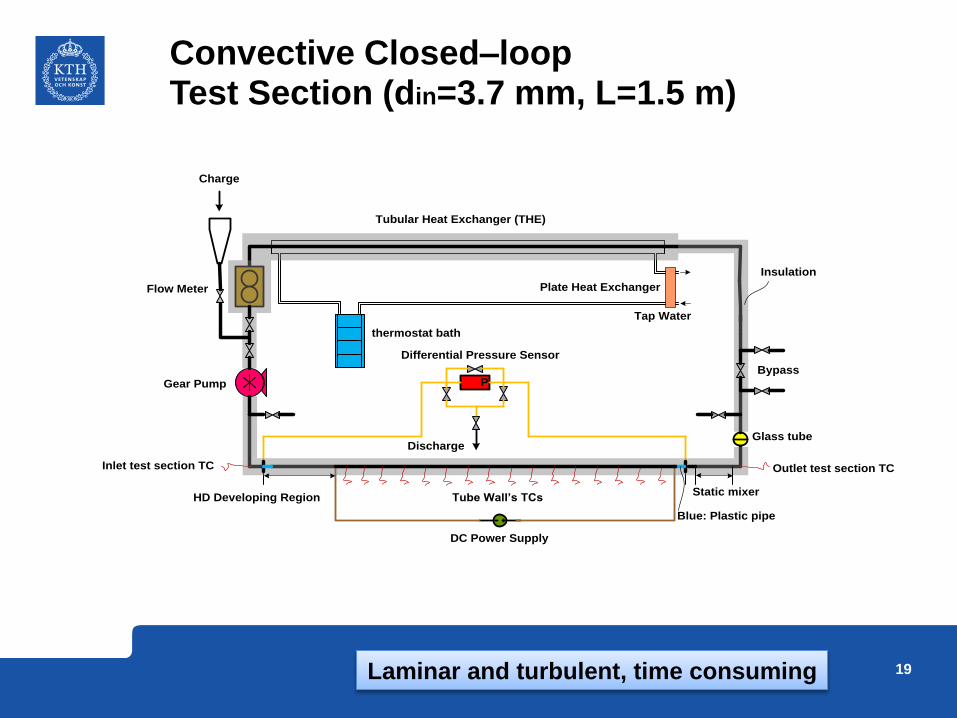
Convective Closed–loop Test Section (din=3.7 mm, L=1.5 m)

P

HD Developing Region

thermostat bath

Gear Pump

Tubular Heat Exchanger (THE)

Plate Heat Exchanger

DC Power Supply

Differential Pressure Sensor

Insulation

Glass tube

Tube Wall’s TCs

Discharge

Tap Water

Charge

Flow Meter

Blue: Plastic pipe

Bypass

Static mixer

Inlet test section TC Outlet test section TC

Laminar and turbulent, time consuming 19

Shelf Stability

20

Material Characterisation

Nanofluid

Source NP Type

Concentration

BFSize

pH

Additives

ItN Nanovation, Germany

Al2O3

(wt%/vol%)

3 – 40 / 1 – 14

DW

9.1

(g surfactant/g solid)

1.5% – 1.8%

Two types

21

Particle Size

Analysis the morphology and dry size of particles

Analysis the hydrodynamic particle size

0

5

10

15

20

25

0 250 500

Inte

ns

ity (

%)

Diameter (nm)

Scanning Electron Microscopy (SEM)

Transmission Electron Microscopy (TEM)

Dynamic Light Scattering (DLS)

22

Al2O3

Al2O3

Additives (Surfactants)

23Source: http://omicsonline.org/2157-7048/2157-7048-2-e101.php

Hydrophobic

Hydrophilic

Base fluid

Theoretical and Empirical Formulas

• Thermophysical Properties

• Pressure Drop and Pumping Power

• Convective Heat Transfer

• Suggested Model

• Stokes’ Law

24

Thermal Conductivity

Maxwell (1873)𝑘𝑛𝑓

𝑘𝑏𝑓=

𝑘𝑝 + 2𝑘𝑏𝑓 + 2 𝑘𝑝 − 𝑘𝑏𝑓 ∅

𝑘𝑝 + 2𝑘𝑏𝑓 − 𝑘𝑝 − 𝑘𝑛𝑓 ∅= 𝑓(𝑘𝑝, 𝑘𝑏𝑓, ∅)

0.0

20.0

40.0

60.0

80.0

0 50 100

kn

f/kb

f

wt. (%)

1.00

1.02

1.04

1.06

1.08

0 50 100 150 200kn

f/kb

f

kp (W/mK)

Al2O3 in DW

25

Viscosity

𝜇𝑛𝑓

𝜇𝑏𝑓= 1 −

∅𝑎∅𝑚

−2.5∅𝑚

= 𝑓(∅, 𝑎, 𝑎𝑎)

∅𝑚 = 0.62, ∅𝑎 = ∅ 𝑎𝑎/𝑎3−𝐷,

𝐷 is typically 1.6 – 2.5 for NFs

𝜇𝑛𝑓

𝜇𝑏𝑓= 1 + 2.5∅ = 𝑓(∅)Einstein (1906)

Modified Krieger–Dougherty (2007)

0.0

2.0

4.0

6.0

8.0

10.0

0 50 100

µn

f/µ

bf

wt. (%)

Einstein

Modified Krieger-Dougherty

𝑎 ⇒ 𝑝𝑎𝑟𝑡𝑖𝑐𝑙𝑒 𝑠𝑖𝑧𝑒𝑎𝑎 ⇒ 𝑎𝑔𝑔𝑟𝑒𝑔𝑎𝑡𝑒 𝑠𝑖𝑧𝑒

Al2O3 in DW26

Density & Specific Heat

Density

Specific Heat

𝜌𝑛𝑓 = ∅𝜌𝑝 + 1 − ∅ 𝜌𝑏𝑓 = 𝑓(𝜌𝑝, 𝜌𝑏𝑓, 𝜙)

𝐶𝑃,𝑛𝑓 =∅𝜌𝑝𝐶𝑃,𝑝 − (1 − ∅)𝜌𝑏𝑓𝐶𝑃,𝑏𝑓

𝜌𝑛𝑓= 𝑓(𝜌𝑝, 𝜌𝑏𝑓, 𝐶𝑃,𝑝, 𝐶𝑃,𝑏𝑓, 𝜙)

0.0

1.0

2.0

3.0

4.0

5.0

0 50 100

ρn

f/ρ

bf

wt. (%)

0.0

0.2

0.4

0.6

0.8

1.0

1.2

0 50 100

Cp

nf/

Cp

bf

wt. (%)

Al2O3 in DW Al2O3 in DW27

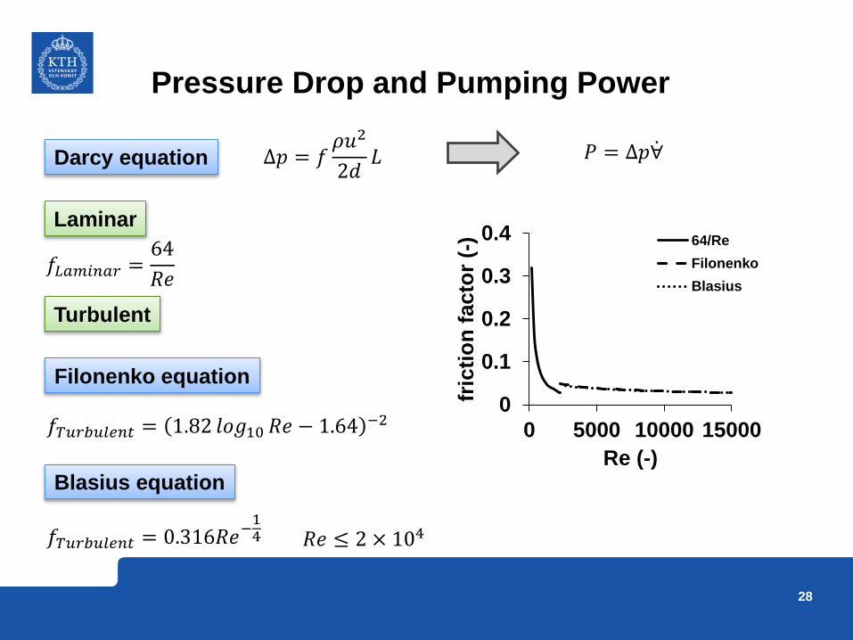
Pressure Drop and Pumping Power

∆𝑝 = 𝑓𝜌𝑢2

2𝑑𝐿Darcy equation

𝑓𝐿𝑎𝑚𝑖𝑛𝑎𝑟 =64

𝑅𝑒

𝑓𝑇𝑢𝑟𝑏𝑢𝑙𝑒𝑛𝑡 = 1.82 𝑙𝑜𝑔10 𝑅𝑒 − 1.64 −2

𝑓𝑇𝑢𝑟𝑏𝑢𝑙𝑒𝑛𝑡 = 0.316𝑅𝑒−14 𝑅𝑒 ≤ 2 × 104

Blasius equation

0

0.1

0.2

0.3

0.4

0 5000 10000 15000

fric

tio

n f

acto

r (-

)Re (-)

64/Re

Filonenko

Blasius

𝑃 = ∆𝑝 ∀

Laminar

Turbulent

Filonenko equation

28

Convective Heat Transfer (Laminar)

𝑁𝑢𝑥 = 𝑓 𝑥∗ , 𝑥∗ =𝑥/𝑑

𝑅𝑒𝑃𝑟𝑁𝑢𝑎𝑣𝑔 = 𝑓(𝐿∗), 𝐿∗ =

𝐿/𝑑

𝑅𝑒𝑃𝑟

4

5

6

7

8

9

10

0 0.1 0.2N

u (

-)

L* (-)

4

5

6

7

8

9

10

0 0.1 0.2

Nu

(-)

x* (-)

Shah (1978) Shah (1975)

29

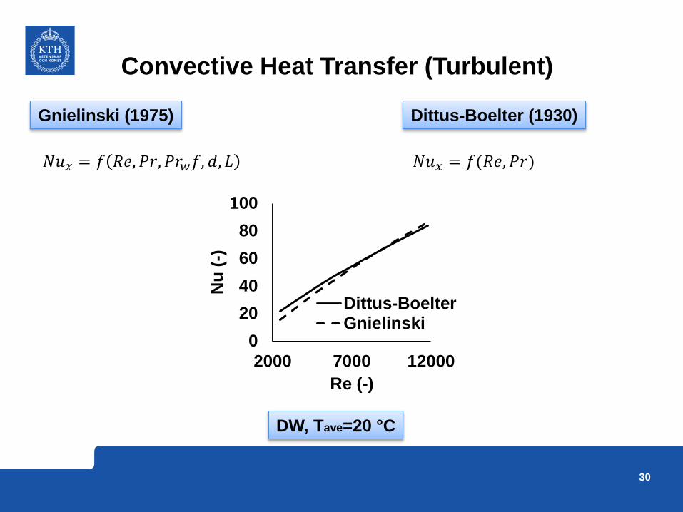
Convective Heat Transfer (Turbulent)

𝑁𝑢𝑥 = 𝑓 𝑅𝑒, 𝑃𝑟, 𝑃𝑟𝑤𝑓, 𝑑, 𝐿 𝑁𝑢𝑥 = 𝑓(𝑅𝑒, 𝑃𝑟)

Gnielinski (1975) Dittus-Boelter (1930)

0

20

40

60

80

100

2000 7000 12000

Nu

(-)

Re (-)

Dittus-BoelterGnielinski

DW, Tave=20 °C

30

Suggested Model

𝑇𝑠−𝑜𝑢𝑡 = 𝑇𝑓−𝑖𝑛 + 𝛥𝑇 + 𝜗

𝑄 = 𝑚𝑐𝑝𝛥𝑇 𝑄 = ℎ𝜗𝐴𝑝

𝑇𝑠−𝑜𝑢𝑡 = 𝑇𝑓−𝑖𝑛 +𝑄

𝑚𝑐𝑝+

𝑄

ℎ𝐴𝑝

𝜆 = (𝑇𝑠−𝑜𝑢𝑡 𝑏𝑓− (𝑇s−𝑜𝑢𝑡 𝑛𝑓

𝜆 = 𝑄1

𝑚𝑐𝑝 𝑏𝑓

1 −𝜌𝑏𝑓

𝜌𝑛𝑓×𝑐𝑝,𝑏𝑓

𝑐𝑝,𝑛𝑓×𝑢𝑏𝑓

𝑢𝑛𝑓+

1

𝜋𝑑𝐿ℎ𝑏𝑓1 −

ℎ𝑏𝑓

ℎ𝑛𝑓

Critical temperature

Tf-in Tf-out

Ts-in Ts-out

Tem

pera

ture

Distance from inlet

Wall

Fluid

ΔT

ν

Includes both thermophysical and transport properties

Positive

Negative

31

Stokes’ Law

𝑢 =𝜌𝑝 − 𝜌𝑓 𝑔𝑑𝑝

2

18𝜇

mg

Fdrag

Fbuoy

32

Summary of Results and Discussion

• Papers 1, 2 and 3: Thermophysical and transport

properties of three NFs

• Paper 4: Cooling performance of NFs in a small-diameter

tube

• Paper 5: Laminar heat transfer in a horizontal tube (closed

loop)

• Paper 6: Turbulent heat transfer in a horizontal tube

(closed loop)

• Paper 7: A method predicting the cooling efficiency of NFs

combining the effect of physical and transport properties

• Paper 8: Shelf stability of NFs and its effect on thermal

conductivity

33

Papers 1, 2 and 3: Thermophysical and transport properties of three NFs

34

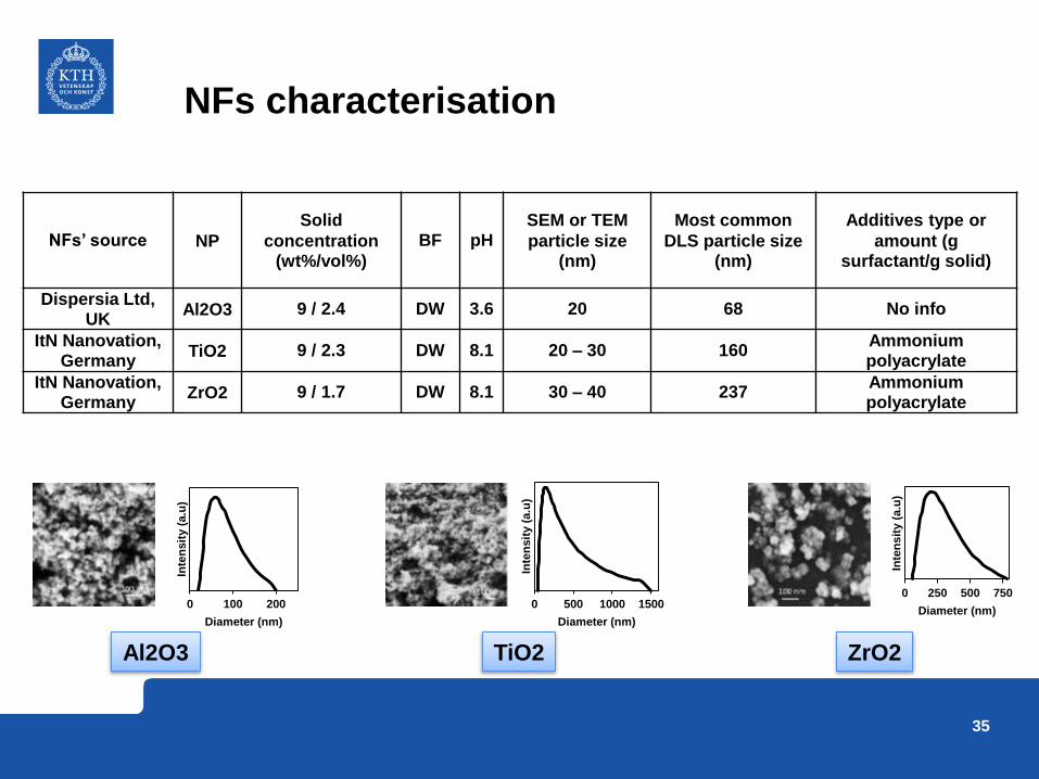
NFs characterisation

NFs’ source NP

Solid

concentration (wt%/vol%)

BF pHSEM or TEM

particle size (nm)

Most common

DLS particle size (nm)

Additives type or

amount (g surfactant/g solid)

Dispersia Ltd, UK

Al2O3 9 / 2.4 DW 3.6 20 68 No info

ItN Nanovation, Germany

TiO2 9 / 2.3 DW 8.1 20 – 30 160Ammonium polyacrylate

ItN Nanovation, Germany

ZrO2 9 / 1.7 DW 8.1 30 – 40 237Ammonium polyacrylate

0 100 200

Inte

ns

ity (

a.u

)

Diameter (nm)

0 500 1000 1500

Inte

nsit

y (

a.u

)

Diameter (nm)

0 250 500 750

Inte

ns

ity (

a.u

)

Diameter (nm)

Al2O3 TiO2 ZrO2

35

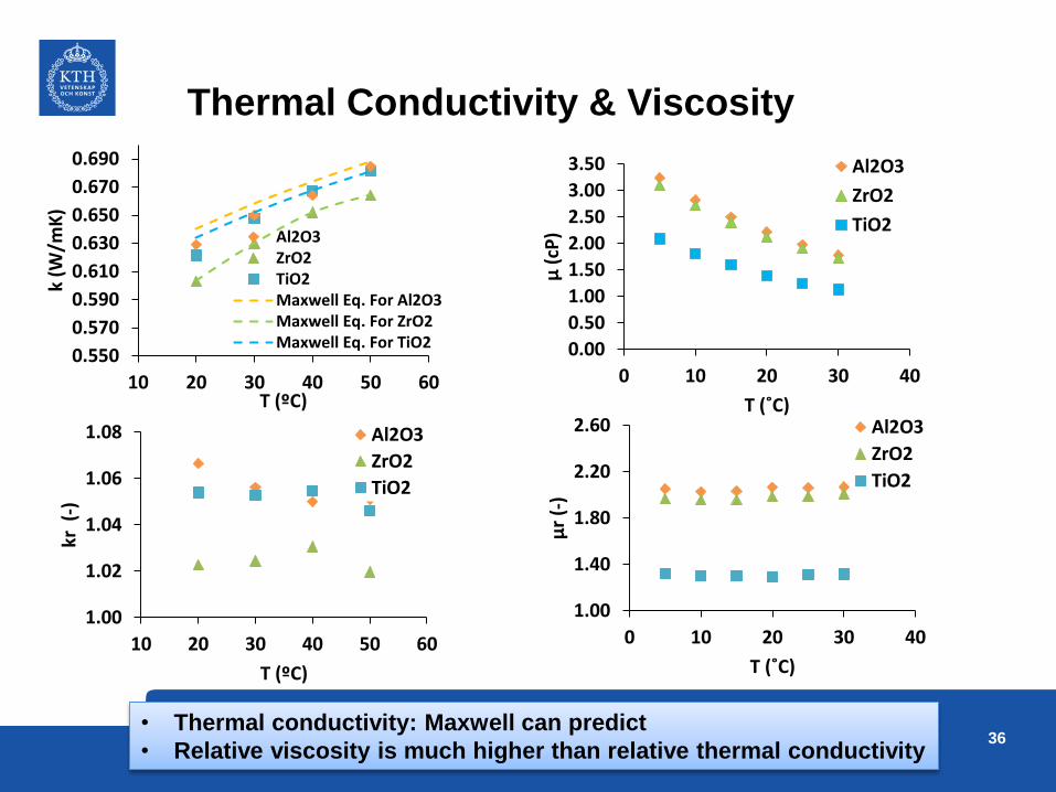
Thermal Conductivity & Viscosity

0.550

0.570

0.590

0.610

0.630

0.650

0.670

0.690

10 20 30 40 50 60

k (W

/mK

)

T (ºC)

Al2O3ZrO2TiO2Maxwell Eq. For Al2O3Maxwell Eq. For ZrO2Maxwell Eq. For TiO2

1.00

1.02

1.04

1.06

1.08

10 20 30 40 50 60

kr (

-)

T (ºC)

Al2O3

ZrO2

TiO2

0.00

0.50

1.00

1.50

2.00

2.50

3.00

3.50

0 10 20 30 40

µ (

cP)

T (˚C)

Al2O3

ZrO2

TiO2

1.00

1.40

1.80

2.20

2.60

0 10 20 30 40

µr

(-)

T (˚C)

Al2O3

ZrO2

TiO2

• Thermal conductivity: Maxwell can predict

• Relative viscosity is much higher than relative thermal conductivity36

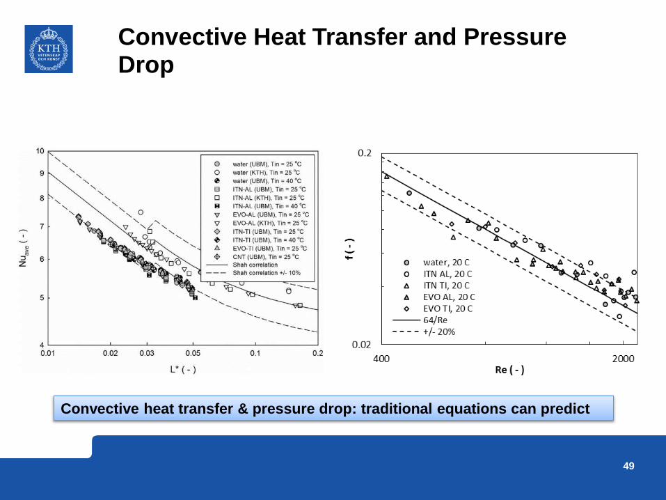
Convective Heat Transfer & Pressure Drop

0

2

4

6

8

10

12

0 500 1000 1500 2000

Nu

(-)

Re (-)

Shah DW Shah TiO2Shah ZrO2 Shah Al2O3DW TiO2ZrO2 Al2O3

0.00

0.05

0.10

0.15

0.20

0.25

0 1000 2000

f (-

)

Re (-)

DWTiO2ZrO2Al2O364/Re64/Re (+/-) 10%

-20

-15

-10

-5

0

5

10

15

20

0 5000 10000

Dev

iati

on

(%

)

Re (-)

DWAl₂O₃TiO₂ZrO₂

Screening set-up Closed Loop

Convective heat transfer & pressure drop:

traditional equations can predict

37

Comparison: Screening Set-up

3000

5000

7000

9000

200 700 1200 1700

h (

W/m

2K

)

Re (-)

3000

5000

7000

9000

10.00 20.00 30.00 40.00

h (

W/m

2K

)

Q (ml/min)

3000

5000

7000

9000

0.500 1.000 1.500 2.000

h (

W/m

2K

)m (kg/hr)

3000

5000

7000

9000

0.2000 0.7000 1.2000

h (

W/m

2K

)

ΔP (Bar)

3000

5000

7000

9000

0.0 20.0 40.0 60.0

h (

W/m

2k)

P (mW)

38

Comparison: Closed Loop

39

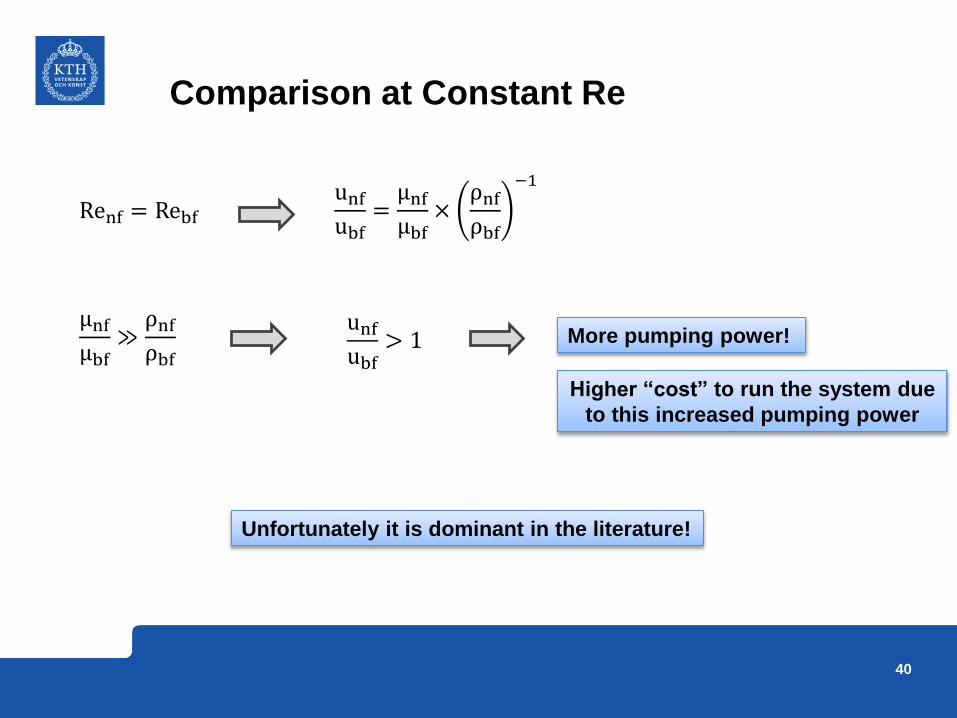
Comparison at Constant Re

Renf = Rebfunfubf

=μnfμbf

×ρnfρbf

−1

μnfμbf

≫ρnfρbf

unfubf

> 1 More pumping power!

Unfortunately it is dominant in the literature!

40

Higher “cost” to run the system due

to this increased pumping power

Comparison at Constant Re

Author Nanofluid Dimension, ReMethod ofComparison

Enhancement of hnf

and comments

Wen and Ding [66]Al2O3/water1.6 vol%

D = 4.5 mm

L = 972Re = 500 – 2100

Same Re47 % near the inlet

region, 14% near the discharge region.

Hwang et al. [67]Al2O3/water0.3 vol%

D = 1.8 mm

L = 2502Re = 400 – 700

Same Re

8% in the developed

region, k increase by

1.44%, viscosity increase by 3%

Rea et al. [68]

Al2O3/water

6 vol%

ZrO2/water1.32 vol%

D = 4.5 mm

L = 1008Re = 140 – 1888

Same velocity

27% for alumina and

3% for zirconia.

Nunf followed single–phase correlation.

Anoop et al. [41]Al2O3/water4 wt%

D = 4.75 mm

L = 1202Re = 700 – 2000

Same Re25% for 45 nm particle

size and 11% for 150 nm particle size.

Liu and Yu [69]Al2O3/water5 vol%

D =1.09 mm

L = 305Re=600 – 4500

Same Re

19% near the entrance

region, 9% near the

discharge region.

Nunf followed single–phase correlation

Vafaei and Wen [70]Al2O3/water1–7 vol%

D = 0.51 mmL = 306

Same velocity

100% at high flow rate,

but no enhancement at low flow rate

He et al. [39]TiO2/water1.1 vol%

D =3.97 mm

L = 1834Re=900 – 5900

Same Re12% in laminar flow and 40% in turbulent flow

Ding et al. [5]CNT/water0.5 wt%

D =4.5 mm

L = 972Re=800 – 1200

Same Re350% in the developed region

Garg et al. [71]CNT/water1 wt%

D =1.55 mm

L = 915Re=600 – 1200

Same Re32% in the developed region

Author Nanofluid Dimension, ReMethod ofComparison

Enhancement of hnf

and comments

Pak and Cho [62]γ-Al2O3/water

and TiO2/water1–3 vol%

D=10.66 mm,

L=4800 mm, Re=104–105

Same velocity

12% lower for γ-Al2O3/water at 3 vol %

He et al. [39]TiO2/water0.2–1.1 vol%

D=3.97 mm,

L=1834 mm, Re=2000–6000

Same ReMaximum 40%

enhancement for 1.1 vol % at Re=5900

Kulkarni [72]

TiO2/(EG–

water 60:40

wt%) 2–10 vol%

D=3.14 mm,

L=1000 mm, Re=3000–12000

Same Re16% enhancement for 10 vol % at Re=10000

Yu et al. [73]SiC/water3.7 vol%

D=2.27 mm, L=580

mm, Re=3300–13000

Same velocity

7% lower

Duangthongsuk and Wongwises [74]

TiO2/water

0.2 – 2.0 vol%

D=9.53 mm,

L=1500 mm,

Re=3000 – 18000

Same Re20–32% enhancement

at 1.0 vol %

Fotukian and Nasr

Esfahany [75]

γ–Al2O3/water

less than 0.2

vol%

D=5 mm, L=1000

mm, Re=6000 –

31000

Same Re48% enhancement at

Re= 10000 and 0.054

vol%

Suresh et al [76]Al2O3/water

0.3 – 0.5 vol%

D=4.85 mm, L=800

mm, Re=700 –

2050

Same Re10 – 48%

enhancement

Fotukian and Nasr

Esfahany [77]

CuO/water

less than 0.24

vol%

D=5 mm, L=1000

mm, Re=6000 –

31000

Same ReMaximum 25%

enhancement

Sajadi and Kazemi

[78]

TiO2/water

less than 0.25

vol%.

D=5 mm, L=1800

mm, Re=5000 –

30000

Same Re~22% enhancement at

Re=5000 and 0.25

vol%

Kayhani et al [79]TiO2/water

0.1 – 2.0 vol%

D=5 mm, L=2000

mm, Re=6000 –

16000

Same Re8% enhancement at

Re= 11800 and 2.0

vol%

Laminar Turbulent

7 out of 9! 8 out of 10!

41

Paper 4: Cooling performance of NFs in a small-diameter tube

42

NFs characterisation

NFs’ source NP

Solid

concentration (wt%/vol%)

BF pH

SEM or

TEM

particle size (nm)

Most

common

DLS

particle size (nm)

Additives type or amount (g surfactant/g solid)

Dispersia Ltd, UK Al2O3 (I) 9 / 2.4 DW 5 ~ 10 180Polyacrylic acid copolymer

sodium salt (0.5 %)

Dispersia Ltd, UK Al2O3 (II) 9 / 2.4 DW 5 ~ 10 60 No additives

Dispersia Ltd TiO2 (I) 9 / 2.3 DW 7.4 20 – 25 170polyacrylic acid

ammonium salt (10.45 %)

ItN Nanovation TiO2 (II) 9 / 2.3 DW 7.4 20 – 25 170polyacrylic acid

ammonium salt (10.45 %)

Nano Grade,

SwitzerlandCeO2 9 / 1.3 DW 7 –8 50 – 100 200 No additives

0.0

1.0

2.0

3.0

4.0

5.0

6.0

0 250 500 750

Dif

f. In

ten

sit

y (

%)

Diameter (nm)

0.0

1.0

2.0

3.0

4.0

5.0

6.0

0 75 150 225

Dif

f. In

ten

sit

y (

%)

Diameter (nm)

0.0

1.0

2.0

3.0

4.0

5.0

6.0

7.0

0 200 400 600

Inte

ns

ity (

%)

Diameter (nm)

0.0

1.0

2.0

3.0

4.0

5.0

6.0

7.0

0 250 500

Inte

ns

ity (

%)

Diameter (nm)

0.0

1.0

2.0

3.0

4.0

5.0

6.0

0 250 500 750

Inte

ns

ity (

%)

Diameter (nm)Al2O3 (I) Al2O3 (II)

TiO2 (I) TiO2 (II)

CeO2

43

Thermal Conductivity & Viscosity

• Thermal conductivity: Maxwell can predict

• Relative viscosity is much higher than relative thermal conductivity

Same conclusion as before

44

Convective Heat Transfer & Pressure Drop

3.0

4.0

5.0

6.0

7.0

8.0

9.0

10.0

0.000 0.100 0.200 0.300

Nu

L*

ShahShah +/- 15%DWAl2O3 (I)Al2O3 (II)TiO2 (I)TiO2 (II)CeO2

0.04

0.06

0.08

0.10

0.12

0.14

0.16

0.18

0.20

200 400 600 800 1000 1200

f

Re

DWAl2O3 (I)Al2O3 (II)TiO2 (I)TiO2 (II)CeO2DarcyDarcy +/- 15%

Convective heat transfer and pressure drop: traditional equations can predict

45

Comparison

4000

4500

5000

5500

6000

6500

7000

200 700 1200

h (

W.m

-2.K

-1)

Re

DWAl2O3 (I)Al2O3 (II)TiO2 (I)TiO2 (II)CeO2

4000

4500

5000

5500

6000

6500

7000

0.5 1.0 1.5

h (

W.m

-2.K

-1)

m (kg/hr)

DWAl2O3 (I)Al2O3 (II)TiO2 (I)TiO2 (II)CeO2

4000

4500

5000

5500

6000

6500

7000

0.5 1.0 1.5 2.0 2.5

h (

W.m

-2.K

-1)

V (m/s)

DWAl2O3 (I)Al2O3 (II)TiO2 (I)TiO2 (II)CeO2

4000

4500

5000

5500

6000

6500

7000

0.0 10.0 20.0 30.0 40.0

h (

W.m

-2.K

-1)

P (mW)

DWAl2O3 (I)Al2O3 (II)TiO2 (I)TiO2 (II)CeO2

46

Paper 5: Laminar heat transfer in a horizontal tube (closed loop)

47

NFs characterisation

NFs’ source NP

Solid

concentration (wt%/vol%)

BF pH

SEM or

TEM

particle size (nm)

Most

common

DLS

particle size (nm)

Additives type or amount (g surfactant/g solid)

ItN Nanovation,

GermanyAl2O3 (I) 9 / 2.4 DW 9.1 100 – 200 200 1.5% – 1.8%

Evonik (Aerodisp

440)Al2O3 (II) 9 / 2.4 DW 4.1 10 – 20 150 1.4 %

ItN Nanovation TiO2 (I) 9 / 2.3 DW 7.8 15 – 50

220 nm or

140 nm

(ultrasonica

ted)

20.8 %

Evonik (Aerodisp

W740X)TiO2 (II) 9 / 2.3 DW 6.7 15 – 50 130 3.0 %

0

5

10

15

20

25

0 500

Inte

ns

ity (

%)

Diameter (nm)

0

5

10

15

20

0 500

Inte

ns

ity (

%)

Diameter (nm)

0

5

10

15

0 500

Inte

ns

ity (

%)

Diameter (nm)

0

5

10

15

0 500

Inte

ns

ity (

%)

Diameter (nm)

Al2O3 (I)

Al2O3 (II)

TiO2 (I)

TiO2 (II)

48

Convective Heat Transfer and Pressure Drop

Convective heat transfer & pressure drop: traditional equations can predict

49

Comparison

50

Paper 6: Turbulent heat transfer in a horizontal tube (closed loop)

51

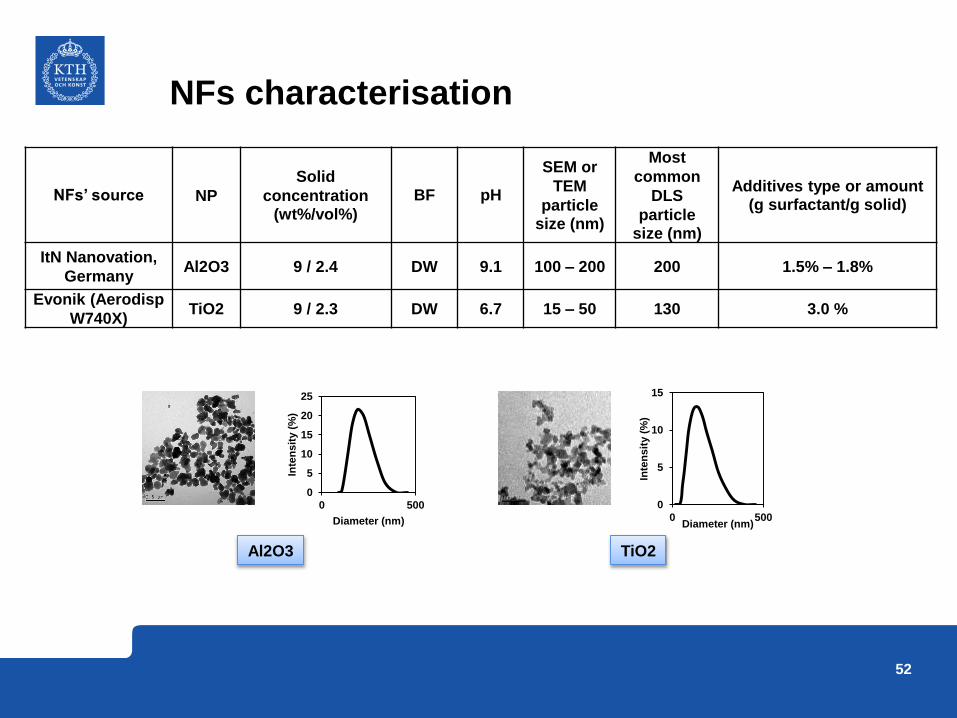
NFs characterisation

NFs’ source NP

Solid

concentration (wt%/vol%)

BF pH

SEM or

TEM

particle size (nm)

Most

common

DLS

particle size (nm)

Additives type or amount (g surfactant/g solid)

ItN Nanovation,

GermanyAl2O3 9 / 2.4 DW 9.1 100 – 200 200 1.5% – 1.8%

Evonik (Aerodisp

W740X)TiO2 9 / 2.3 DW 6.7 15 – 50 130 3.0 %

0

5

10

15

20

25

0 500

Inte

ns

ity (

%)

Diameter (nm)

0

5

10

15

0 500

Inte

ns

ity (

%)

Diameter (nm)

Al2O3 TiO2

52

Thermal Conductivity & Viscosity

• Thermal conductivity: Maxwell can predict

• Relative viscosity is much higher than relative thermal conductivity

Same conclusion as before

53

Convective Heat Transfer

0

20

40

60

80

2000 4000 6000 8000 10000

Nu

(-)

Re (-)

KTH (Al₂O₃)UBHAM (Al₂O₃)GnielinskiGnielinski +/- 10%

0

20

40

60

80

2000 4000 6000 8000 10000

Nu

(-)

Re (-)

KTH (Al₂O₃)UBHAM (Al₂O₃)GnielinskiGnielinski +/- 10%

0

20

40

60

80

2000 4000 6000 8000 10000

Nu

(-)

Re (-)

KTH (TiO₂)UBHAM (TiO₂)GnielinskiGnielinski +/- 10%

0

20

40

60

80

2000 4000 6000 8000 10000

Nu

(-)

Re (-)

KTH (TiO₂)UBHAM (TiO₂)GnielinskiGnielinski +/- 10%

25 °C

40 °C

25 °C

40 °C

Convective heat transfer: traditional equations can predict 54

Pressure Drop

0.02

0.03

0.04

0.05

0.06

4000 6000 8000 10000

f (-

)

Re (-)

KTH (DW)KTH (Al₂O₃) KTH (TiO₂)FilonenkoFilonenko +/- 10%

Pressure drop: traditional equations can predict

55

Comparison

-5

0

5

10

15

20

3000 4500 6000 7500 9000

Incr

eas

e (

%)

Re (-)

-5

0

5

10

15

20

3000 4500 6000 7500 9000

Incr

eas

e (

%)

Re (-)

-25

-20

-15

-10

-5

0

5

10

0 500 1000

Incr

eas

e (

%)

P (mW)

-25

-20

-15

-10

-5

0

5

10

0 500 1000

Incr

eas

e (

%)

P (mW)

25 °C

40 °C

25 °C

40 °C

56

Paper 7: A method predicting the cooling efficiency of NFs combining the effect of physical and transport properties

57

NFs characterisation

NFs’ source NP

Solid

concentration (wt%/vol%)

BF pH

SEM or

TEM

particle size (nm)

Most common

DLS particle size (nm)

Additives type or

amount (g surfactant/g solid)

ItN Nanovation,

Germany

Al2O3

(ITN-AL)3 – 40 / 1 – 14 DW 9.1 100 – 200 200 1.5% – 1.8%

Evonik (Aerodisp

440)

Al2O3

(EVO-AL)3 – 40 / 1 – 17 DW 4.1 10 – 20 150 1.4 %

Alafa Aesar

(Nanodur X1121W)

Al2O3

(AA-AL)3 – 40 / 1 – 14 DW 4.0 10 – 80 160 12.7 %

ItN NanovationTiO2

(ITN-TI)3 – 20 / 1 – 6 DW 7.8 15 – 50

220 nm or

140 nm

(ultrasonicated)

20.8 %

Evonik (Aerodisp

W740X)

TiO2

(EVO-TI)3 – 40 / 1 – 15 DW 6.7 15 – 50 130 3.0 %

Eka Chemical

Levasil 100SiO2

(LEVASIL-SI)3 – 45 / 1 – 27 DW 10

30 nm

spherical90 0 %

Alfa Aesar (Nanotek

CE6042)CeO2

(AA-CI)3 – 20 / 0.5 – 3 DW 2.5

30 nm

(cubic)160 0.5 %

58

Thermal Conductivity (1)

1.0

1.1

1.2

1.3

1.4

1.5

1.6

0.0 10.0 20.0 30.0 40.0

kr-E

xp

wt.%

EVO-AL (KTH)EVO-AL (UBHAM)ITN-AL (KTH)ITN-AL (UBHAM)AA-AL (KTH)AA-AL (UBHAM)EVO-TI (KTH)EVO-TI (UBHAM)ITN-TI (KTH)ITN-TI (UBHAM)LEVASIL-SI (KTH)LEVASIL-SI (UBHAM)AA-CI (KTH)AA-CI (UBHAM)

1.0

1.1

1.2

1.3

1.4

1.5

1.6

1.0 1.1 1.2 1.3 1.4 1.5 1.6

kr-E

xp

kr-Maxwell

EVO-AL (KTH)EVO-AL (UBHAM)ITN-AL (KTH)ITN-AL (UBHAM)AA-AL (KTH)AA-AL (UBHAM)EVO-TI (KTH)EVO-TI (UBHAM)ITN-TI (KTH)ITN-TI (UBHAM)LEVASIL-SI (KTH)LEVASIL-SI (UBHAM)AA-CI (KTH)AA-CI (UBHAM)kr-Exp=kr-Maxwell(+/-) 10%

20 °C

59

Thermal Conductivity (2)

1.00

1.05

1.10

1.15

10 20 30 40 50 60

kr-E

xp

T (˚C)

EVO-ALITN-ALAA-ALEVO-TIITN-TILEVASIL-SIAA-CI

1.00

1.05

1.10

1.15

1.00 1.05 1.10 1.15kr

-Exp

kr-Maxwell

EVO-ALITN-ALAA-ALEVO-TIITN-TILEVASIL-SIAA-CIkr-Exp=kr-Maxwell(+/-) 10%

60

9 wt%

Viscosity (1)

1.0

2.0

3.0

4.0

5.0

6.0

7.0

8.0

0.0 10.0 20.0 30.0 40.0

µr-

Exp

wt.%

EVO-AL (KTH)EVO-AL (UBHAM)ITN-AL (KTH)ITN-AL (UBHAM)AA-AL (KTH)AA-AL (UBHAM)EVO-TI (KTH)EVO-TI (UBHAM)ITN-TI (KTH)ITN-TI (UBHAM)LEVASIL-SI (KTH)LEVASIL-SI (UBHAM)AA-CI (KTH)AA-CI (UBHAM)

1.0

2.0

3.0

4.0

5.0

6.0

7.0

8.0

1.0 3.0 5.0 7.0

µr-

Exp

µr-KD

EVO-AL (KTH)EVO-AL (UBHAM)ITN-AL (KTH)ITN-AL (UBHAM)AA-AL (KTH)AA-AL (UBHAM)EVO-TI (KTH)EVO-TI (UBHAM)ITN-TI (KTH)ITN-TI (UBHAM)LEVASIL-SI (KTH)LEVASIL-SI (UBHAM)AA-CI (KTH)AA-CI (UBHAM)µr-Exp=µr-KD(+/-) 10%

20 °C

61

Viscosity (2)

1.0

1.1

1.2

1.3

1.4

1.5

1.6

10 20 30 40 50

µ-r

el-

Exp

T (˚C)

EVO-ALITN-ALAA-ALEVO-TIITN-TILEVASIL-SIAA-CI

1.0

1.1

1.2

1.3

1.4

1.5

1.6

1.0 1.2 1.4 1.6

µ-r

el-

Exp

µ-rel-KD

EVO-ALITN-ALAA-ALEVO-TIITN-TILEVASIL-SIAA-CIµr-Exp=µr-KD(+/-) 10%

62

9 wt%

Thermal Conductivity & Viscosity

• Thermal conductivity: Maxwell can predict even at elevated temperature

• Viscosity: modified Krieger–Dougherty can predict even at elevated temperature

• Relative viscosity is much higher than relative thermal conductivity

63

Comparison

-1.0

0.0

1.0

2.0

3.0

0 10 20 30

λ (˚

C)

wt.%

Equal Re

Equal V

Equal P

-1.0

0.0

1.0

2.0

3.0

0 10 20 30

λ (˚

C)

wt.%

Equal Re

Equal V

Equal P

Laminar Turbulent

ITN-AL

64

𝜆 = 𝑄1

𝑚𝑐𝑝 𝑏𝑓

1 −𝜌𝑏𝑓

𝜌𝑛𝑓×𝑐𝑝,𝑏𝑓

𝑐𝑝,𝑛𝑓×𝑢𝑏𝑓

𝑢𝑛𝑓+

1

𝜋𝑑𝐿ℎ𝑏𝑓1 −

ℎ𝑏𝑓

ℎ𝑛𝑓

Paper 8: Shelf stability of NFs and its effect on thermal conductivity

65

NFs characterisation

NFs’ source NP

Solid

concentrati

on (wt%/vol%)

BF pH

SEM or

TEM

particle size (nm)

Most

common

DLS particle size (nm)

Additives type or

amount (g surfactant/g solid)

Clay I (CPI, UK) Clay (I) 9 / 3.8 DW 8 – 8.5 20 – 40* 1420 No info

Clay II (CPI, UK) Clay (II) 9 / 2.7 DW 8 – 8.5 40 – 400 490 No info

Clay III

(ItN Nanovation, Germany) Clay (III) 1.75 / 0.4 DW 7 80 – 250 320 No additives

ItN Nanovation, Germany Al2O3 9 / 2.4 DWNo

info40 – 200 220 No info

0

1

2

3

4

5

0 2000 4000 6000

Inte

nsi

ty (

%)

Diameter (nm)

0

2

4

6

8

10

0 200 400 600 800

Inte

nsi

ty (

%)

Diameter (nm)

0

2

4

6

8

10

12

0 200 400

Inte

nsi

ty (

%)

Diameter (nm)

0

2

4

6

8

10

0 200 400 600

%In

ten

sity

Diameter (nm)

Clay (I) Clay (II)

Clay (III) Al2O3

66

Sedimentation and Sedimentation Rate

67

Photography Method

A sample of photographs for of

Clay (I), (II) and (III) NFs at the

beginning (a), after 30 minutes (b),

1 hour (c), 5 hours (d), 10 hours

(e), 20 hours (f), 30 hours (g) and

40 hours (h) of measurement

After eight days

Clay (I), (II), (III)

68

Sedimentation and Sedimentation Rate Al2O3

69

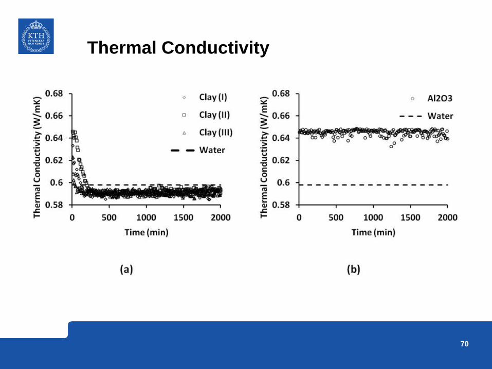
Thermal Conductivity

70

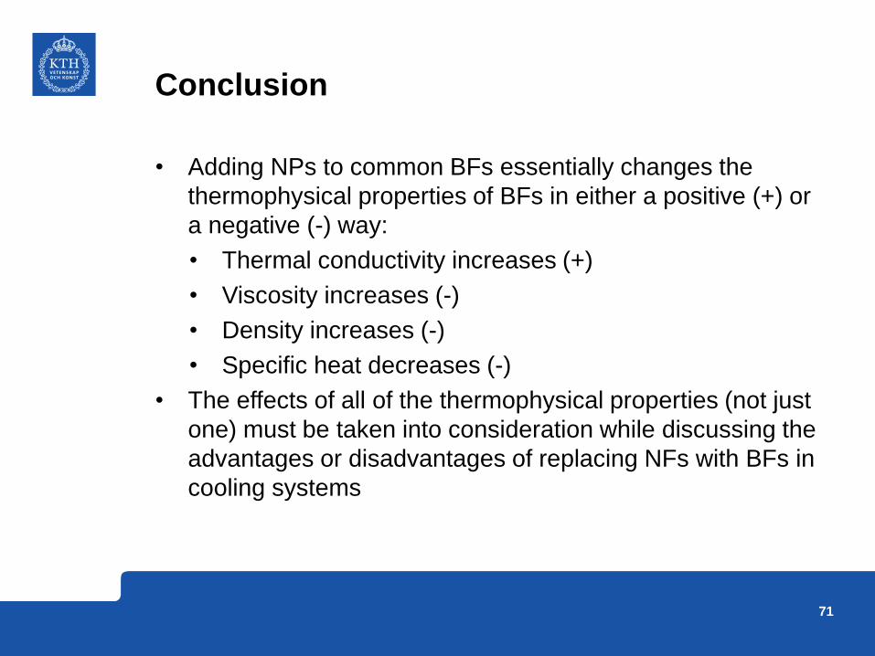
Conclusion

• Adding NPs to common BFs essentially changes the

thermophysical properties of BFs in either a positive (+) or

a negative (-) way:

• Thermal conductivity increases (+)

• Viscosity increases (-)

• Density increases (-)

• Specific heat decreases (-)

• The effects of all of the thermophysical properties (not just

one) must be taken into consideration while discussing the

advantages or disadvantages of replacing NFs with BFs in

cooling systems

71

Conclusion

• The Maxwell model can predict thermal conductivity of

most of the NFs tested within 10% uncertainty

• The modified Krieger–Dougherty (K-D) model can predict

the viscosity of most of these NFs within 10% error

• The success of (K-D) model is highly dependent on

knowing the ratio of aggregated to primary particles, as

well as on an experimental determination of another

variable called the fractional index

• When correct thermophysical properties, either from

experiments or trustable models, are used, the classical

correlations traditionally used for common fluids are still

valid for NFs with acceptable error

72

Conclusion

• Mechanisms such as nanoparticle migration due to Brownian motion or thermophoresis seem to have negligible effects on thermophysical and transport properties of NFs

• Comparing the results at the same Reynolds numbers, although the most popular method employed in the literature, is not relevant in practical applications

• The evaluation of the heat transfer performance of the NFs at equal pumping power is the most appropriate and correct approach from an industrial point of view

• Based on this criterion, the experimental results of this study show only a small benefit for some NFs in laminar flow for cooling applications. In turbulent flow, however, NFs evidenced no benefit at all

73

Conclusion

• To quickly check the feasibility of replacing BFs with NFs,

a method of analysis was suggested based on the

calculation of the highest wall temperature in a heat sink

• The applicability of the sedimentation balance method to

analysing the sedimentation behaviour of NFs was

illustrated successfully

• Commercialisation of NFs for cooling applications is still a

relevant question

• The focus of future research must move towards the

material synthesis of NFs with the purpose to reduce the

viscosity increases experienced by BFs due to the addition

of NPs

74

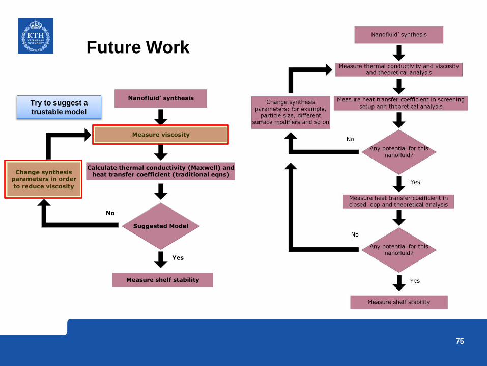
Future Work

Nanofluid synthesis

Measure viscosity

Calculate thermal conductivity (Maxwell) and heat transfer coefficient (traditional eqns)

Suggested Model

Change synthesis parameters in order to reduce viscosity

Yes

No

Measure shelf stability

Try to suggest a

trustable model

75

76