simulation of the guirguis cylinder experiment using...
TRANSCRIPT
Simulation of the Guirguis cylinder experiment using coupled Chinook/LS-DYNA
Liam Gannon DRDC Atlantic Research Centre
Defence Research and Development Canada Scientific Report DRDC-RDDC-2017-R002 January 2017

IMPORTANT INFORMATIVE STATEMENTS Template in use: SR Advanced Template_EN (110414).dot
© Her Majesty the Queen in Right of Canada, as represented by the Minister of National Defence, 2017
© Sa Majesté la Reine (en droit du Canada), telle que représentée par le ministre de la Défense nationale, 2017
DRDC-RDDC-2017-R002 i
Abstract ……..
A methodology for simulating the response of structures to the shockwave produced by close-proximity underwater explosions (UNDEX) is demonstrated using the Chinook hydrocode coupled with the LS-DYNA explicit dynamics finite element (FE) code. The simulation reproduces an experiment wherein a 2.8 g charge of pentaerythritol tetranitrate (PETN) is detonated inside a water-filled aluminum cylinder. The secondary loading resulting from reflection of the shockwave off of the gas bubble as a rarefaction wave is reproduced along with consequent reloading of the structure due cavitation closure in the fluid. The simulation results are in good agreement with experimental measurements of structural deformation and pressure at the inner wall of the cylinder. The predicted peak radial deformation of the cylinder wall at the mid-height is within 5.5% of the measured value.
Significance to defence and security
Comparison of simulation results with experimental measurements demonstrates the accuracy with which close-proximity UNDEX events can be simulated using the most up-to-date tools and highlights areas where improvements can be made. The lessons learned can be applied to future close-proximity UNDEX research, working towards predicting damage to full-scale ship and submarine structures subjected to close-proximity UNDEX. The ultimate goal is to develop the ability to assess and improve the vulnerability of existing and proposed naval platforms.

ii DRDC-RDDC-2017-R002
This page intentionally left blank.
DRDC-RDDC-2017-R002 iii
Résumé ……..
Grâce à l'hydrocode Chinook et au code d'éléments finis dynamiques explicites LS-DYNA, on a validé une méthode de simulation de la réaction de structures à des ondes de choc produites par des explosions sous-marines à proximité immédiate. La simulation visait à reproduire une expérience au cours de laquelle on a fait détoner une charge de 2,8 g de tétranitrate de pentaérythritol (PETN) dans un contenant cylindrique d'aluminium rempli d'eau. Lors de cette expérience, on a simulé la charge secondaire issue de la réflexion, sous forme d'onde de raréfaction, de l'onde de choc par les bulles de gaz, ainsi que la recharge de la structure consécutive à la fermeture des cavités dans le fluide. Les résultats de la simulation concordent bien avec les mesures de la pression et de la déformation structurales prises pendant l'expérience à la hauteur de la paroi interne du contenant. La simulation a permis de prévoir la déformation radiale maximale de la paroi du contenant à mi-hauteur à 5,5 % près de la valeur mesurée.
Importance pour la défense et la sécurité
En comparant les résultats de la simulation aux mesures prises durant l'expérience, on a démontré l'exactitude avec laquelle on peut simuler des explosions sous-marines à proximité immédiate à l'aide des plus récents outils et on a souligné les améliorations pouvant être apportées. Les leçons tirées pourront servir lors de futurs travaux de recherche en la matière en vue de prévoir les dommages causés aux navires et aux structures sous-marines « grandeur réelle » soumis à des explosions sous-marines à proximité immédiate. Le but ultime consiste à pouvoir évaluer et réduire la vulnérabilité des plateformes navales existantes et envisagées.

iv DRDC-RDDC-2017-R002
This page intentionally left blank.
DRDC-RDDC-2017-R002 v
Table of contents
Abstract …….. ................................................................................................................................. i Significance to defence and security ................................................................................................ i Résumé …….. ................................................................................................................................ iii Importance pour la défense et la sécurité ....................................................................................... iii Table of contents ............................................................................................................................. v
List of figures ................................................................................................................................. vi List of tables .................................................................................................................................. vii 1 Introduction ............................................................................................................................... 1
1.1 Background ...................................................................................................................... 1
1.2 Description of the experiment ......................................................................................... 2
2 Methodology ............................................................................................................................. 3
2.1 Fluid model ...................................................................................................................... 3
2.2 Finite element model ....................................................................................................... 8
3 Results ..................................................................................................................................... 10
3.1 Variation of explosive EOS parameters ........................................................................ 10
3.2 Tait versus Tillotson EOS for water .............................................................................. 14
3.3 Variation of finite element type ..................................................................................... 16
3.4 Small and large deformation coupling ........................................................................... 17
3.5 Axisymmetric Model ..................................................................................................... 20
4 Conclusion .............................................................................................................................. 21
5 References ............................................................................................................................... 25
List of symbols/abbreviations/acronyms/initialisms ..................................................................... 27
vi DRDC-RDDC-2017-R002
List of figures
Figure 1: Guirguis hydro-bulged cylinder experiment. ................................................................... 2
Figure 2: 2D fluid cell size convergence. ........................................................................................ 4
Figure 3: 2D fluid domain (water in cylinder is green, air is blue). ................................................ 5
Figure 4: 3D fluid domain (quarter cylinder filled with water, surrounded by air). ........................ 5
Figure 5: Density-pressure relationships for Tait and Tillotson equations of state. ........................ 7
Figure 6: Cylinder shell (left) and solid (right) FE models (quarter symmetry). ............................ 9
Figure 7: Resultant displacement (5x magnification) for PETN JWL parameters from [15]. ...... 10
Figure 8: Radial displacement at cylinder mid-height. .................................................................. 11
Figure 9: Absolute pressure contours from simulation using JWL parameters from [15]. ........... 12
Figure 10: Time-history of absolute pressure on inner wall at cylinder mid-height. .................... 13
Figure 11: Time-history of velocity at cylinder mid-height. ......................................................... 13
Figure 12: Wall cavitation at 30 μs – JWL parameters from [15]. ................................................ 14
Figure 13: Radial deflection using Tillotson and Tait equations of state. ..................................... 15
Figure 14: Pressure at mid-height using Tillotson and Tait equations of state.............................. 15
Figure 15: Radial displacement time-histories for solid and shell models. ................................... 17
Figure 16: Small and large deformation coupling radial displacement comparison. .................... 18
Figure 17: Small and large deformation coupling radial velocity comparison.............................. 19
Figure 18: Small and large deformation coupling pressure comparison. ...................................... 19
Figure 19: Resultant displacement from axisymmetric simulation (displacement scale factor x10). ............................................................................................................................ 20

DRDC-RDDC-2017-R002 vii
List of tables
Table 1: Equation of state parameters. ............................................................................................ 7
Table 2: Zerilli-Armstrong parameters for 5083 Al [5]. ................................................................. 8
Table 3: Maximum radial displacements. ...................................................................................... 17

This page intentionally left blank.
viii DRDC-RDDC-2017-R002
DRDC-RDDC-2017-R002 1
1 Introduction
1.1 Background
The ability to withstand explosion damage and maintain the ability to float, move and fight is a key consideration in the design and protection of naval platforms. Where explosions in air and far-field underwater explosions are concerned, there are well-established methods of calculating their effects on nearby structures [1], [2]. With close-proximity underwater explosions (UNDEX) however, there are added complications due to the presence of the bubble containing the gaseous products of the explosion. These include reflections of the shockwave off of the structure and the gas bubble, motion of the gas bubble and jetting of water through the bubble as it collapses toward the structure. When detonation occurs at a standoff distance large enough that the bubble does not attach to the structure, the sequence of events is as follows:
Following detonation, the shockwave reaches the structure causing rapid deformation, reducing the fluid pressure at the surface of the structure, potentially causing cavitation at the fluid-structure interface.
The reflected shockwave reaches the gas bubble boundary and is reflected from the bubble surface as a rarefaction (reduction in density) wave. This causes a reduction in fluid pressure between the structure and bubble boundary contributing to the already reduced pressure due to motion of the structure.
The structure is reloaded by collapse of the low pressure region between the bubble boundary and structure surface.
In a previous attempt to validate the ability of the Chinook hydrocode coupled with the LS-DYNA finite element analysis (FEA) code to simulate close-proximity UNDEX events, the size of the fluid grid and limitations of software functionalities were problematic in obtaining realistic behaviour [1]. The fluid flow and shockwave behaviour were not resolved accurately enough to produce bubble migration and jetting towards the structure. As a result, the structural deformation was not accurately predicted. In this report, only the initial stages of an UNDEX event, described above, are simulated. The absence of bubble migration and jetting in the experiment used for comparison simplifies the analysis, and the shorter run-time required allows for faster evaluation of various analysis options in both the Chinook and LS-DYNA codes.
In this report, simulations of the Guirguis hydro-bulged cylinder experiment are compared with experimental data in order to assess the validity of the simulation methodology. Simulation parameters are varied in an effort to understand the influence of different modeling practices on solution accuracy. These include the effect of finite element type (solid versus shell), finite element formulation, variations in explosive equation of state (EOS) parameters, variation of water EOS type and the type of coupling between the fluid and structure. Hydrocode predictions of damage in the Guirguis hydro-bulged cylinder experiments have previously been presented by Wardlaw et al. [3] and Wardlaw and Luton [4], who used methods similar to the present study, i.e., an Eulerian fluid/explosive model coupled with a Lagrangian structural finite element model. Techniques for deformation measurement along with measurement data are given by Sandusky
2 DRDC-RDDC-2017-R002
et al. [5] and techniques for pressure measurement and pressure data are presented by Chambers et al. [6].
1.2 Description of the experiment
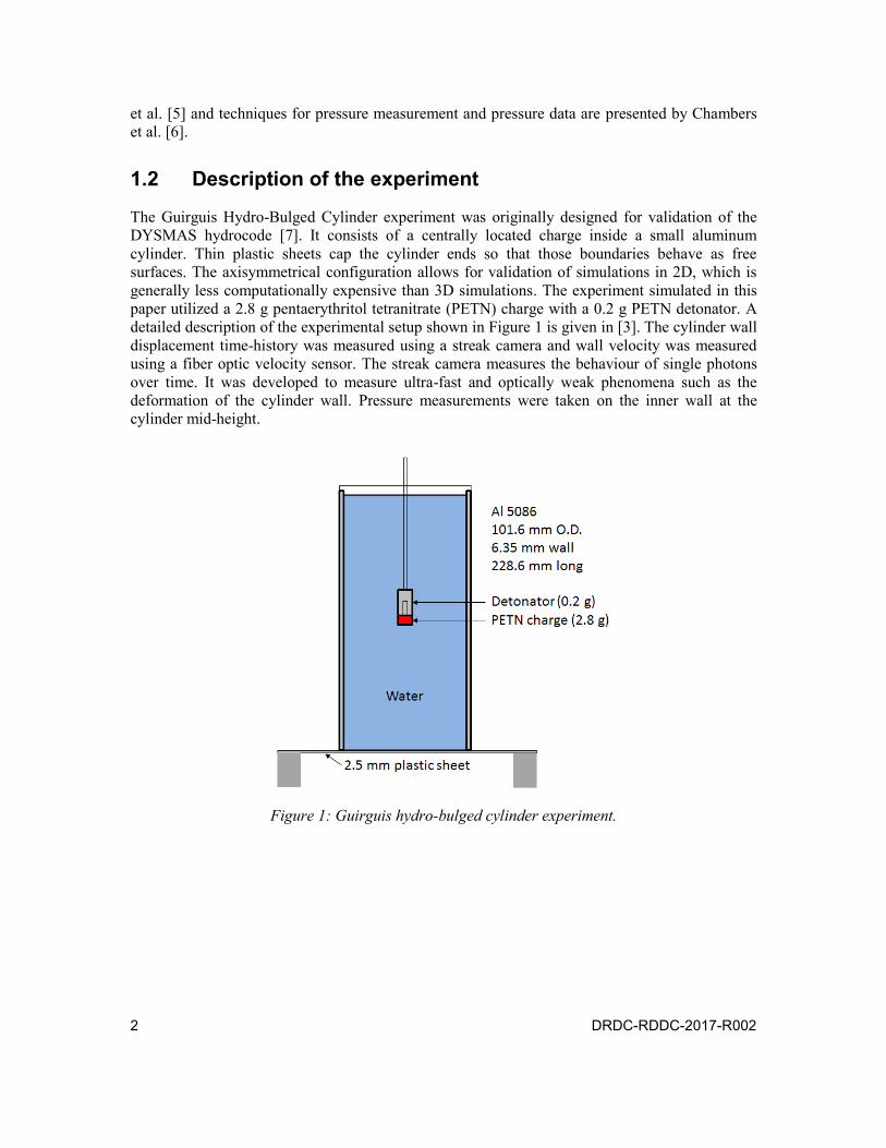
The Guirguis Hydro-Bulged Cylinder experiment was originally designed for validation of the DYSMAS hydrocode [7]. It consists of a centrally located charge inside a small aluminum cylinder. Thin plastic sheets cap the cylinder ends so that those boundaries behave as free surfaces. The axisymmetrical configuration allows for validation of simulations in 2D, which is generally less computationally expensive than 3D simulations. The experiment simulated in this paper utilized a 2.8 g pentaerythritol tetranitrate (PETN) charge with a 0.2 g PETN detonator. A detailed description of the experimental setup shown in Figure 1 is given in [3]. The cylinder wall displacement time-history was measured using a streak camera and wall velocity was measured using a fiber optic velocity sensor. The streak camera measures the behaviour of single photons over time. It was developed to measure ultra-fast and optically weak phenomena such as the deformation of the cylinder wall. Pressure measurements were taken on the inner wall at the cylinder mid-height.
Figure 1: Guirguis hydro-bulged cylinder experiment.
DRDC-RDDC-2017-R002 3
2 Methodology
The fluid dynamics within the cylinder are simulated using the Chinook Eulerian hydrocode [8] and the structural response is calculated using the LS-DYNA explicit dynamics solver [9]. Pressures from the fluid calculation are passed to the structure and the velocity (and optionally, position) of the structure at the fluid-structure interface is passed back to the fluid model. The simulation is started in the 2D fluid domain with no consideration of fluid structure interaction and run until the shockwave has almost reached the inner wall of the cylinder. At that point, the fluid domain pressures (and velocities, etc.) are mapped from the 2D domain to a 3D domain and the simulation is continued in 3D with fluid-structure interaction. This allows for the use of a higher fidelity fluid model as the shockwave is propagated than is practical to use in 3D. The benefits are that diffusion of the shockwave due to discretization of the fluid domain is reduced. Also, the run time to simulate shockwave propagation to the fluid-structure interface may be reduced because fewer elements may be used and the dimensionality of the advection calculation is reduced. However, the computational time saved by using fewer elements is partially offset by the smaller time step that must be used with the smaller grid cells in the 2D model. All simulations were run using Chinook version 195 unless otherwise noted.
Modeling of the fluid and structure can be approached in several ways and there are also a number of different sets of equation of state parameters for the PETN explosive available in literature. In order to understand which modeling practices and material descriptions best represent the physics of the experiment, the following variations are investigated:
The structure is modelled with both solid and shell elements, considering different shell element formulations.
The simulation is run with and without accounting for large deformation coupling at the fluid-structure interface. With large deformation coupling enabled, the Computational fluid dynamics (CFD) calculation accounts for the movement of the fluid-structure interface as the structure deforms.
Different sets of explosive EOS parameters are compared.
Two different equations of state for water are compared.
3D versus axisymmetric fluid domain model.
2.1 Fluid model
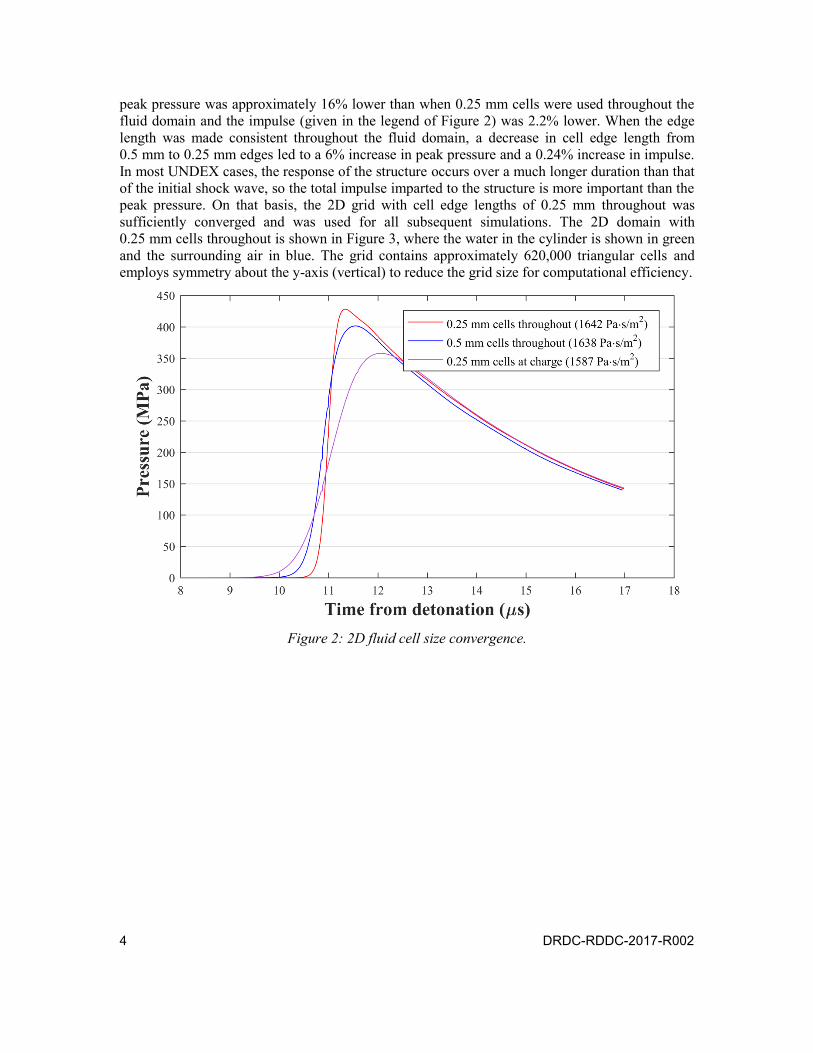
A convergence study was performed to determine the density required of the 2D fluid grid (created using the Pointwise software [10]) in order to prevent significant diffusion of the shockwave before mapping the results to the 3D domain. Figure 3 shows pressure time-histories at the cylinder mid-height 1 cm away from the inner wall for three grids: one with 0.25 mm cell edge lengths throughout; one with 0.5 mm edge lengths throughout; and one with 0.25 mm cells at the charge location, increasing to 1 mm at the cylinder inner wall. In the third case, there was noticeable diffusion of the shockwave as a result of the coarser grid near the cylinder wall. The
4 DRDC-RDDC-2017-R002
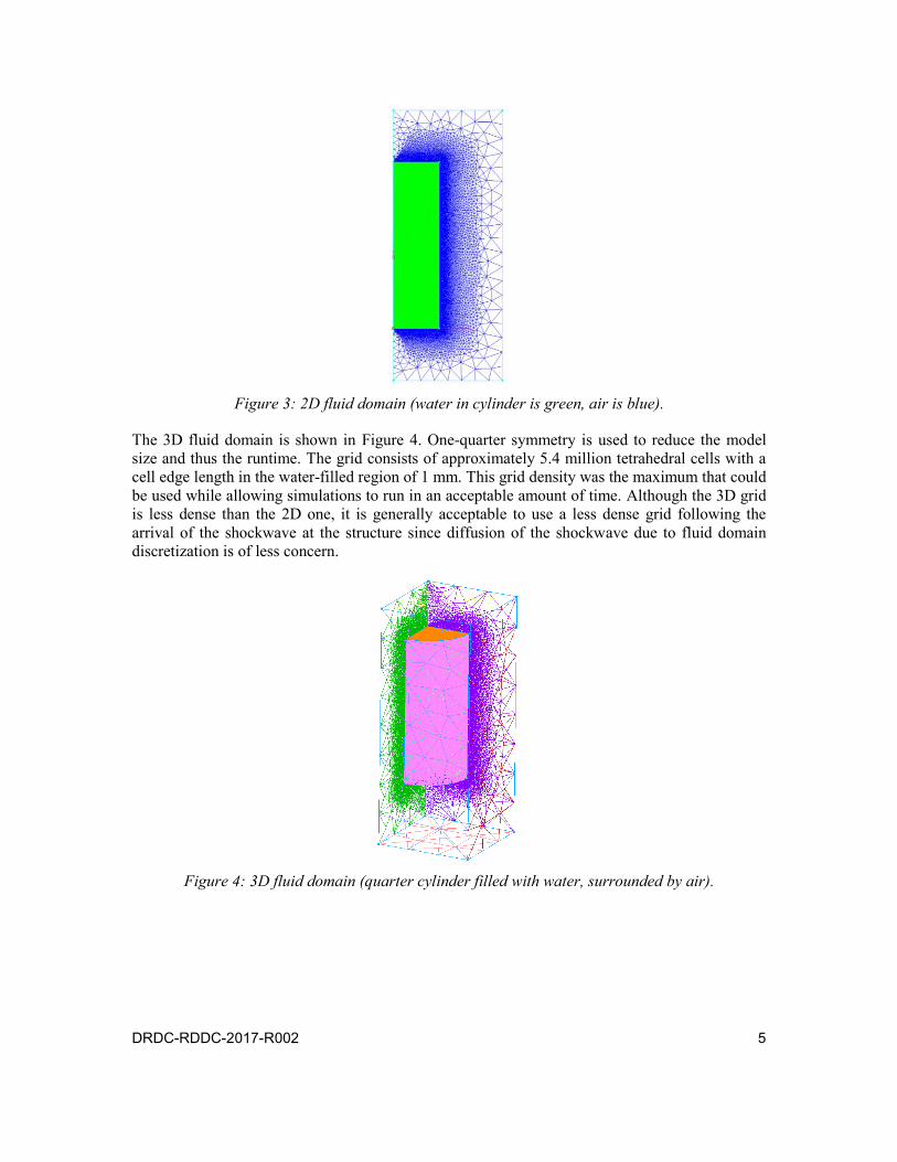
peak pressure was approximately 16% lower than when 0.25 mm cells were used throughout the fluid domain and the impulse (given in the legend of Figure 2) was 2.2% lower. When the edge length was made consistent throughout the fluid domain, a decrease in cell edge length from 0.5 mm to 0.25 mm edges led to a 6% increase in peak pressure and a 0.24% increase in impulse. In most UNDEX cases, the response of the structure occurs over a much longer duration than that of the initial shock wave, so the total impulse imparted to the structure is more important than the peak pressure. On that basis, the 2D grid with cell edge lengths of 0.25 mm throughout was sufficiently converged and was used for all subsequent simulations. The 2D domain with 0.25 mm cells throughout is shown in Figure 3, where the water in the cylinder is shown in green and the surrounding air in blue. The grid contains approximately 620,000 triangular cells and employs symmetry about the y-axis (vertical) to reduce the grid size for computational efficiency.
Figure 2: 2D fluid cell size convergence.
DRDC-RDDC-2017-R002 5
Figure 3: 2D fluid domain (water in cylinder is green, air is blue).
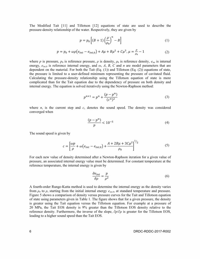
The 3D fluid domain is shown in Figure 4. One-quarter symmetry is used to reduce the model size and thus the runtime. The grid consists of approximately 5.4 million tetrahedral cells with a cell edge length in the water-filled region of 1 mm. This grid density was the maximum that could be used while allowing simulations to run in an acceptable amount of time. Although the 3D grid is less dense than the 2D one, it is generally acceptable to use a less dense grid following the arrival of the shockwave at the structure since diffusion of the shockwave due to fluid domain discretization is of less concern.
Figure 4: 3D fluid domain (quarter cylinder filled with water, surrounded by air).
6 DRDC-RDDC-2017-R002
The Modified Tait [11] and Tillotson [12] equations of state are used to describe the pressure-density relationship of the water. Respectively, they are given by
𝑝 = 𝑝0 [(𝐵 + 1) (
𝜌
𝜌0)𝑛
− 𝐵] (1)
𝑝 = 𝑝0 +𝜔𝜌(𝑒𝑖𝑛𝑡 − 𝑒𝑖𝑛𝑡,0) + 𝐴𝜇 + 𝐵𝜇2 + 𝐶𝜇3, 𝜇 =
𝜌
𝜌0− 1 (2)
where p is pressure, p0 is reference pressure, ρ is density, ρ0 is reference density, eint is internal energy, eint,0 is reference internal energy, and ω, A, B, C and n are model parameters that are dependent on the material. For both the Tait (Eq. (1)) and Tillotson (Eq. (2)) equations of state, the pressure is limited to a user-defined minimum representing the pressure of cavitated fluid. Calculating the pressure-density relationship using the Tillotson equation of state is more complicated than for the Tait equation due to the dependency of pressure on both density and internal energy. The equation is solved iteratively using the Newton-Raphson method:
𝑝𝑛+1 = 𝑝𝑛 +
(𝑝 − 𝑝𝑛)
(𝑐𝑛)2 (3)
where n, is the current step and c, denotes the sound speed. The density was considered converged when
(𝑝 − 𝑝𝑛)
𝑝< 10−5 (4)
The sound speed is given by
𝑐 = [
𝜔𝑝
𝜌+ 𝜔(𝑒𝑖𝑛𝑡 − 𝑒𝑖𝑛𝑡,0) +
𝐴 + 2𝐵𝜇 + 3𝐶𝜇2
𝜌0]
12⁄
(5)
For each new value of density determined after a Newton-Raphson iteration for a given value of pressure, an associated internal energy value must be determined. For constant temperature at the reference temperature, the internal energy is given by
𝜕𝑒𝑖𝑛𝑡𝜕𝜌
=𝑝
𝜌2 (6)
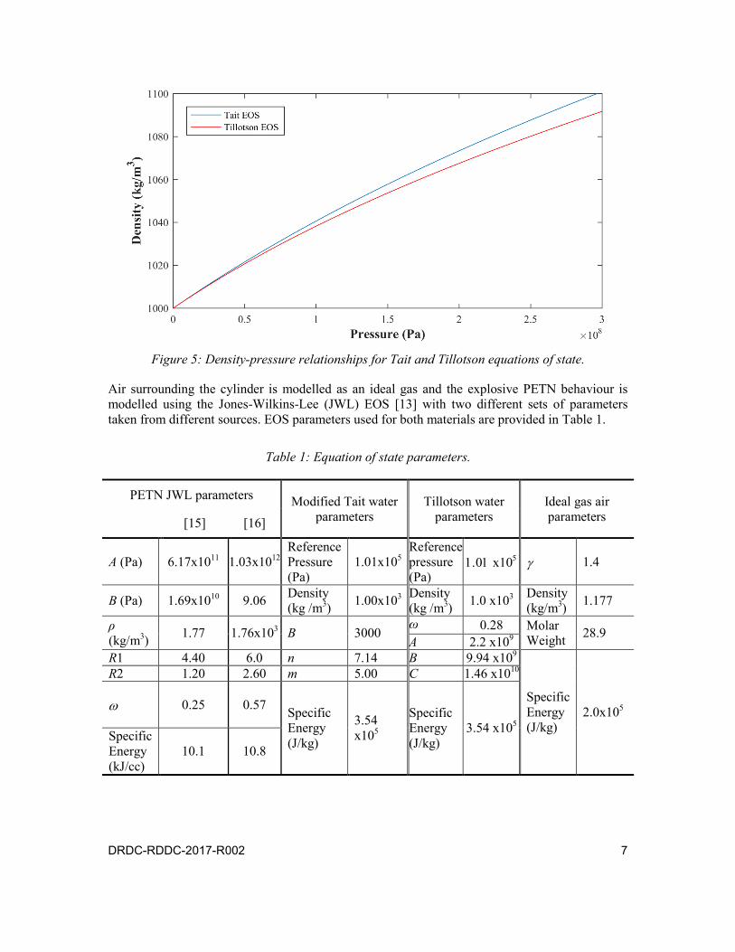
A fourth-order Runge-Kutta method is used to determine the internal energy as the density varies from ρ0 to ρ, starting from the initial internal energy eint,0, at standard temperature and pressure. Figure 5 shows a comparison of density versus pressure curves for the Tait and Tillotson equation of state using parameters given in Table 1. The figure shows that for a given pressure, the density is greater using the Tait equation versus the Tillotson equation. For example at a pressure of 20 MPa, the Tait EOS density is 9% greater than the Tillotson EOS density relative to the reference density. Furthermore, the inverse of the slope, ∂p/∂ρ is greater for the Tillotson EOS, leading to a higher sound speed than the Tait EOS.
DRDC-RDDC-2017-R002 7
Figure 5: Density-pressure relationships for Tait and Tillotson equations of state.
Air surrounding the cylinder is modelled as an ideal gas and the explosive PETN behaviour is modelled using the Jones-Wilkins-Lee (JWL) EOS [13] with two different sets of parameters taken from different sources. EOS parameters used for both materials are provided in Table 1.
Table 1: Equation of state parameters.
PETN JWL parameters Modified Tait water parameters
Tillotson water parameters
Ideal gas air parameters [15] [16]
A (Pa) 6.17x10¹¹ 1.03x10¹² Reference Pressure (Pa)
1.01x10⁵ Reference pressure (Pa)
x10 1.4
B (Pa) 1.69x10¹⁰ 9.06 Density (kg /m3) 1.00x10³ Density
(kg /m3) 1.0 x10³ Density (kg/m3) 1.177
ρ (kg/m3) 1.77 1.76x10³ B 3000
ω 0.28 Molar Weight 28.9
A 2.2 x10⁹ R1 4.40 6.0 n 7.14 B 9.94 x10⁹
Specific Energy (J/kg)
2.0x10⁵
R2 1.20 2.60 m 5.00 C 1.46 x10¹⁰
0.25 0.57 Specific Energy (J/kg)
3.54 x10⁵
Specific Energy (J/kg)
3.54 x10⁵ Specific Energy (kJ/cc)
10.1 10.8
8 DRDC-RDDC-2017-R002
2.2 Finite element model
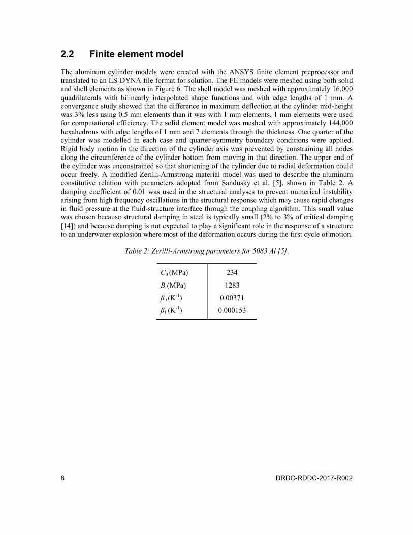
The aluminum cylinder models were created with the ANSYS finite element preprocessor and translated to an LS-DYNA file format for solution. The FE models were meshed using both solid and shell elements as shown in Figure 6. The shell model was meshed with approximately 16,000 quadrilaterals with bilinearly interpolated shape functions and with edge lengths of 1 mm. A convergence study showed that the difference in maximum deflection at the cylinder mid-height was 3% less using 0.5 mm elements than it was with 1 mm elements. 1 mm elements were used for computational efficiency. The solid element model was meshed with approximately 144,000 hexahedrons with edge lengths of 1 mm and 7 elements through the thickness. One quarter of the cylinder was modelled in each case and quarter-symmetry boundary conditions were applied. Rigid body motion in the direction of the cylinder axis was prevented by constraining all nodes along the circumference of the cylinder bottom from moving in that direction. The upper end of the cylinder was unconstrained so that shortening of the cylinder due to radial deformation could occur freely. A modified Zerilli-Armstrong material model was used to describe the aluminum constitutive relation with parameters adopted from Sandusky et al. [5], shown in Table 2. A damping coefficient of 0.01 was used in the structural analyses to prevent numerical instability arising from high frequency oscillations in the structural response which may cause rapid changes in fluid pressure at the fluid-structure interface through the coupling algorithm. This small value was chosen because structural damping in steel is typically small (2% to 3% of critical damping [14]) and because damping is not expected to play a significant role in the response of a structure to an underwater explosion where most of the deformation occurs during the first cycle of motion.
Table 2: Zerilli-Armstrong parameters for 5083 Al [5].
C0 (MPa) 234
B (MPa) 1283
β0 (K-1) 0.00371
β1 (K-1) 0.000153
DRDC-RDDC-2017-R002 9
Figure 6: Cylinder shell (left) and solid (right) FE models (quarter symmetry).
10 DRDC-RDDC-2017-R002
3 Results
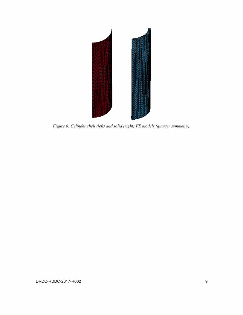
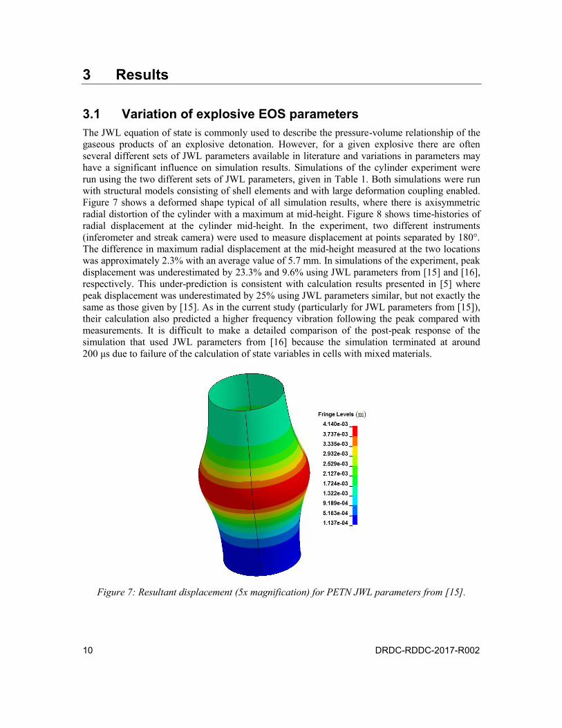
3.1 Variation of explosive EOS parameters The JWL equation of state is commonly used to describe the pressure-volume relationship of the gaseous products of an explosive detonation. However, for a given explosive there are often several different sets of JWL parameters available in literature and variations in parameters may have a significant influence on simulation results. Simulations of the cylinder experiment were run using the two different sets of JWL parameters, given in Table 1. Both simulations were run with structural models consisting of shell elements and with large deformation coupling enabled. Figure 7 shows a deformed shape typical of all simulation results, where there is axisymmetric radial distortion of the cylinder with a maximum at mid-height. Figure 8 shows time-histories of radial displacement at the cylinder mid-height. In the experiment, two different instruments (inferometer and streak camera) were used to measure displacement at points separated by 180°. The difference in maximum radial displacement at the mid-height measured at the two locations was approximately 2.3% with an average value of 5.7 mm. In simulations of the experiment, peak displacement was underestimated by 23.3% and 9.6% using JWL parameters from [15] and [16], respectively. This under-prediction is consistent with calculation results presented in [5] where peak displacement was underestimated by 25% using JWL parameters similar, but not exactly the same as those given by [15]. As in the current study (particularly for JWL parameters from [15]), their calculation also predicted a higher frequency vibration following the peak compared with measurements. It is difficult to make a detailed comparison of the post-peak response of the simulation that used JWL parameters from [16] because the simulation terminated at around 200 μs due to failure of the calculation of state variables in cells with mixed materials.
Figure 7: Resultant displacement (5x magnification) for PETN JWL parameters from [15].
DRDC-RDDC-2017-R002 11
Figure 8: Radial displacement at cylinder mid-height.
Figure 9 shows contours of fluid pressure at a series of times during the simulation where JWL parameters from [15] were used. The white regions in the figure denote areas where the pressure has fallen below atmospheric pressure (101,325 Pa). The figure shows (a) the pressure distribution at the time at which it is mapped from 2D to 3D; (b) the reflection of the shockwave off of the inner wall of the cylinder; (c) a region of cavitation between the surface of the gaseous explosion products and the inner surface of the cylinder caused by reflection of the shockwave from the bubble surface as a rarefaction; (d) collapse of the cavitated region; (e) the resulting shockwave; (f) the impact of the cavitation closure shockwave on the inner wall of the cylinder; (g) its reflection off the cylinder wall; and (h) regions of reduced pressure in the surrounding air indicating the onset of numerical instability in the solution.
Figure 10 shows pressure time-histories from the experiment [3] and from simulations using both sets of JWL parameters, where the data set shown in red corresponds to the contours in Figure 9. The peak pressure measured in the experiment was approximately 637 MPa whereas the simulation peak pressure was 557 MPa for both sets of JWL parameters. This difference is not unexpected, as there is typically some diffusion of the shockwave due to discretization of the fluid domain. The small difference between the beginning of the pressure rise in the experiment and simulations is attributed to the difference between the experimental time datum (initiation of detonation) and the simulation start time (detonation is complete and the explosive has been converted into its gaseous products). The time of arrival of the cavitation closure pulse at the cylinder wall is 91 μs, compared to approximately 84 μs and 72 μs for simulations with JWL parameters from [15] and [16], respectively. The earlier increase in pressure observed in the measured data at 65 μs was not captured in the simulations. That pressure increase may have been a result of the collapse of a layer of cavitation at the cylinder wall following its initial outward motion. An associated increase in wall velocity between 60 μs and 80 μs was measured during the experiment, as shown in Figure 11. This increase in velocity due to wall cavitation collapse was not reproduced in the simulations where, even though a low pressure region was formed at the
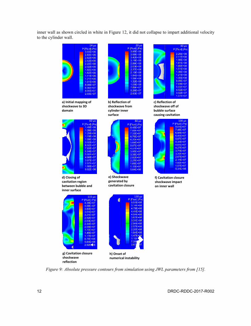
12 DRDC-RDDC-2017-R002
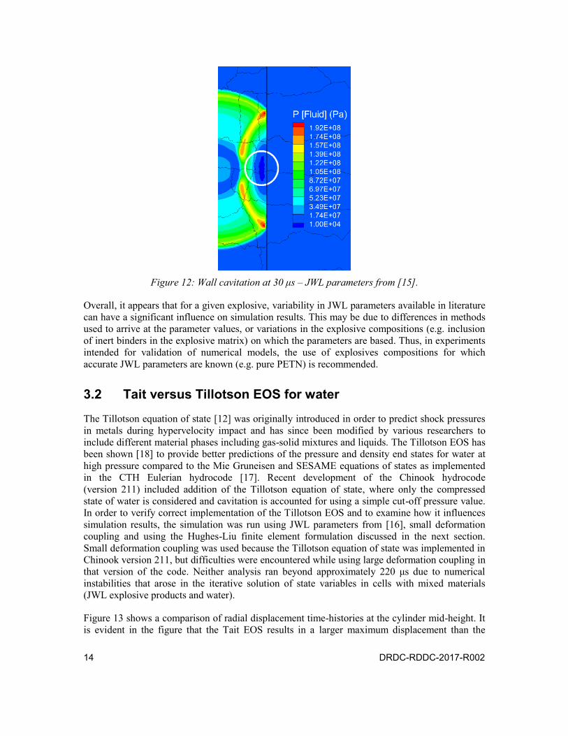
inner wall as shown circled in white in Figure 12, it did not collapse to impart additional velocity to the cylinder wall.
Figure 9: Absolute pressure contours from simulation using JWL parameters from [15].
14 μs 20 μs 40 μs
80 μs 100 μs
115 μs
a) Initial mapping of shockwave to 3D domain
b) Reflection of shockwave from cylinder inner surface
60 μs
c) Reflection of shockwave off of bubble surface causing cavitation
d) Closing of cavitation region between bubble and inner surface
e) Shockwave generated by cavitation closure
130 μs
f) Cavitation closure shockwave impact on inner wall
g) Cavitation closure shockwave reflection
h) Onset of numerical instability
130 μs
DRDC-RDDC-2017-R002 13
Figure 10: Time-history of absolute pressure on inner wall at cylinder mid-height.
Figure 11: Time-history of velocity at cylinder mid-height.
14 DRDC-RDDC-2017-R002
Figure 12: Wall cavitation at 30 μs – JWL parameters from [15].
Overall, it appears that for a given explosive, variability in JWL parameters available in literature can have a significant influence on simulation results. This may be due to differences in methods used to arrive at the parameter values, or variations in the explosive compositions (e.g. inclusion of inert binders in the explosive matrix) on which the parameters are based. Thus, in experiments intended for validation of numerical models, the use of explosives compositions for which accurate JWL parameters are known (e.g. pure PETN) is recommended.
3.2 Tait versus Tillotson EOS for water
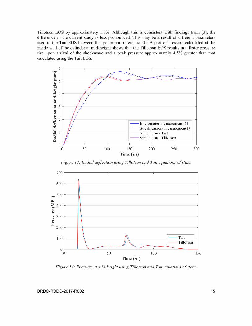
The Tillotson equation of state [12] was originally introduced in order to predict shock pressures in metals during hypervelocity impact and has since been modified by various researchers to include different material phases including gas-solid mixtures and liquids. The Tillotson EOS has been shown [18] to provide better predictions of the pressure and density end states for water at high pressure compared to the Mie Gruneisen and SESAME equations of states as implemented in the CTH Eulerian hydrocode [17]. Recent development of the Chinook hydrocode (version 211) included addition of the Tillotson equation of state, where only the compressed state of water is considered and cavitation is accounted for using a simple cut-off pressure value. In order to verify correct implementation of the Tillotson EOS and to examine how it influences simulation results, the simulation was run using JWL parameters from [16], small deformation coupling and using the Hughes-Liu finite element formulation discussed in the next section. Small deformation coupling was used because the Tillotson equation of state was implemented in Chinook version 211, but difficulties were encountered while using large deformation coupling in that version of the code. Neither analysis ran beyond approximately 220 μs due to numerical instabilities that arose in the iterative solution of state variables in cells with mixed materials (JWL explosive products and water).
Figure 13 shows a comparison of radial displacement time-histories at the cylinder mid-height. It is evident in the figure that the Tait EOS results in a larger maximum displacement than the
DRDC-RDDC-2017-R002 15
Tillotson EOS by approximately 1.5%. Although this is consistent with findings from [3], the difference in the current study is less pronounced. This may be a result of different parameters used in the Tait EOS between this paper and reference [3]. A plot of pressure calculated at the inside wall of the cylinder at mid-height shows that the Tillotson EOS results in a faster pressure rise upon arrival of the shockwave and a peak pressure approximately 4.5% greater than that calculated using the Tait EOS.
Figure 13: Radial deflection using Tillotson and Tait equations of state.
Figure 14: Pressure at mid-height using Tillotson and Tait equations of state.
16 DRDC-RDDC-2017-R002
3.3 Variation of finite element type
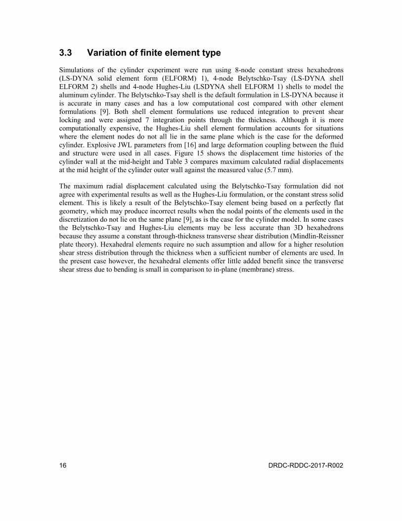
Simulations of the cylinder experiment were run using 8-node constant stress hexahedrons (LS-DYNA solid element form (ELFORM) 1), 4-node Belytschko-Tsay (LS-DYNA shell ELFORM 2) shells and 4-node Hughes-Liu (LSDYNA shell ELFORM 1) shells to model the aluminum cylinder. The Belytschko-Tsay shell is the default formulation in LS-DYNA because it is accurate in many cases and has a low computational cost compared with other element formulations [9]. Both shell element formulations use reduced integration to prevent shear locking and were assigned 7 integration points through the thickness. Although it is more computationally expensive, the Hughes-Liu shell element formulation accounts for situations where the element nodes do not all lie in the same plane which is the case for the deformed cylinder. Explosive JWL parameters from [16] and large deformation coupling between the fluid and structure were used in all cases. Figure 15 shows the displacement time histories of the cylinder wall at the mid-height and Table 3 compares maximum calculated radial displacements at the mid height of the cylinder outer wall against the measured value (5.7 mm).
The maximum radial displacement calculated using the Belytschko-Tsay formulation did not agree with experimental results as well as the Hughes-Liu formulation, or the constant stress solid element. This is likely a result of the Belytschko-Tsay element being based on a perfectly flat geometry, which may produce incorrect results when the nodal points of the elements used in the discretization do not lie on the same plane [9], as is the case for the cylinder model. In some cases the Belytschko-Tsay and Hughes-Liu elements may be less accurate than 3D hexahedrons because they assume a constant through-thickness transverse shear distribution (Mindlin-Reissner plate theory). Hexahedral elements require no such assumption and allow for a higher resolution shear stress distribution through the thickness when a sufficient number of elements are used. In the present case however, the hexahedral elements offer little added benefit since the transverse shear stress due to bending is small in comparison to in-plane (membrane) stress.
DRDC-RDDC-2017-R002 17
Figure 15: Radial displacement time-histories for solid and shell models.
Table 3: Maximum radial displacements.
Finite element type
Element formulation (LS-DYNA ELFORM)
Maximum radial displacement (mm)
Difference from experiment (%)
Solid Constant stress (1) 5.33 6.49
Shell Belytschko-Tsay (2) 5.14 9.82
Shell Hughes-Liu (1) 5.39 5.44
3.4 Small and large deformation coupling
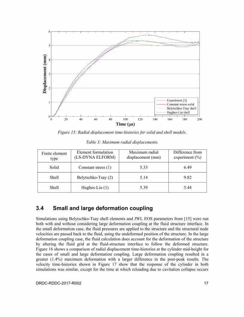
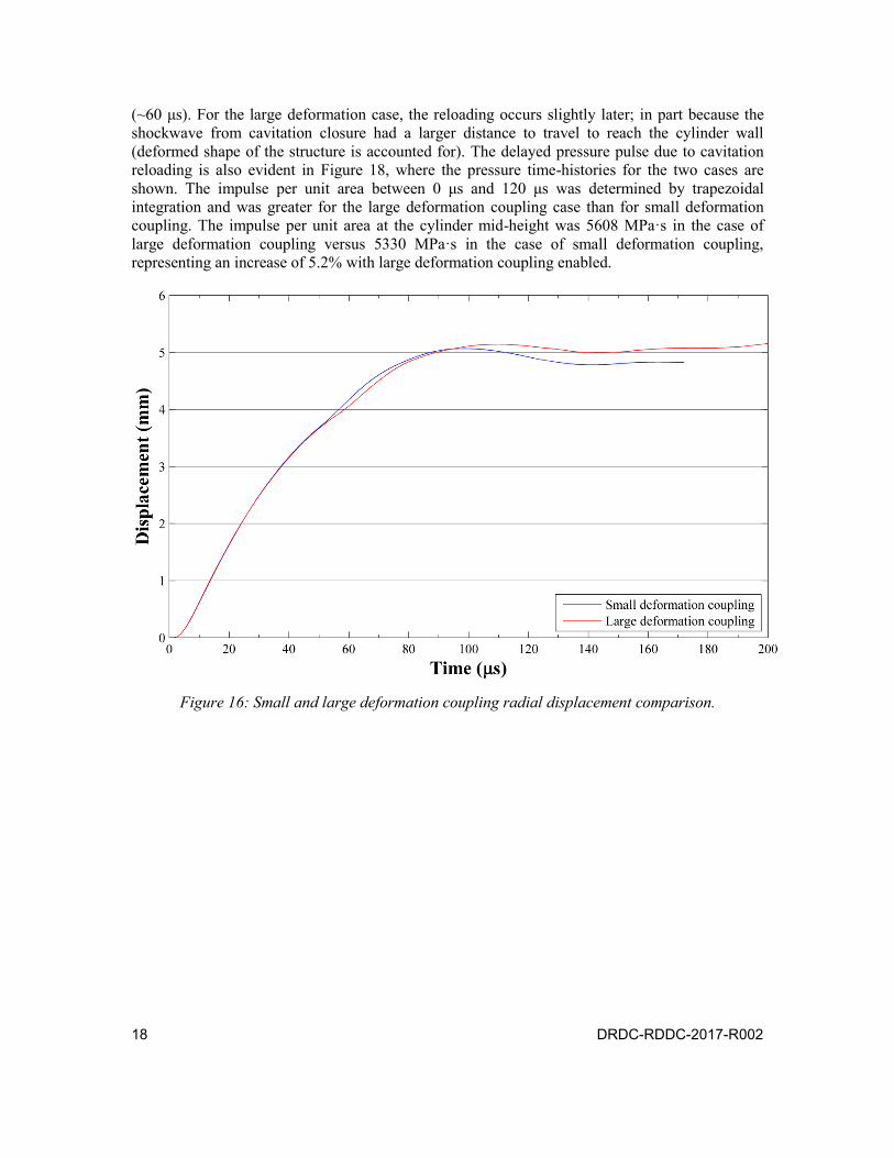
Simulations using Belytschko-Tsay shell elements and JWL EOS parameters from [15] were run both with and without considering large deformation coupling at the fluid structure interface. In the small deformation case, the fluid pressures are applied to the structure and the structural node velocities are passed back to the fluid, using the undeformed position of the structure. In the large deformation coupling case, the fluid calculation does account for the deformation of the structure by altering the fluid grid at the fluid-structure interface to follow the deformed structure. Figure 16 shows a comparison of radial displacement time-histories at the cylinder mid-height for the cases of small and large deformation coupling. Large deformation coupling resulted in a greater (1.4%) maximum deformation with a larger difference in the post-peak results. The velocity time-histories shown in Figure 17 show that the response of the cylinder in both simulations was similar, except for the time at which reloading due to cavitation collapse occurs
18 DRDC-RDDC-2017-R002
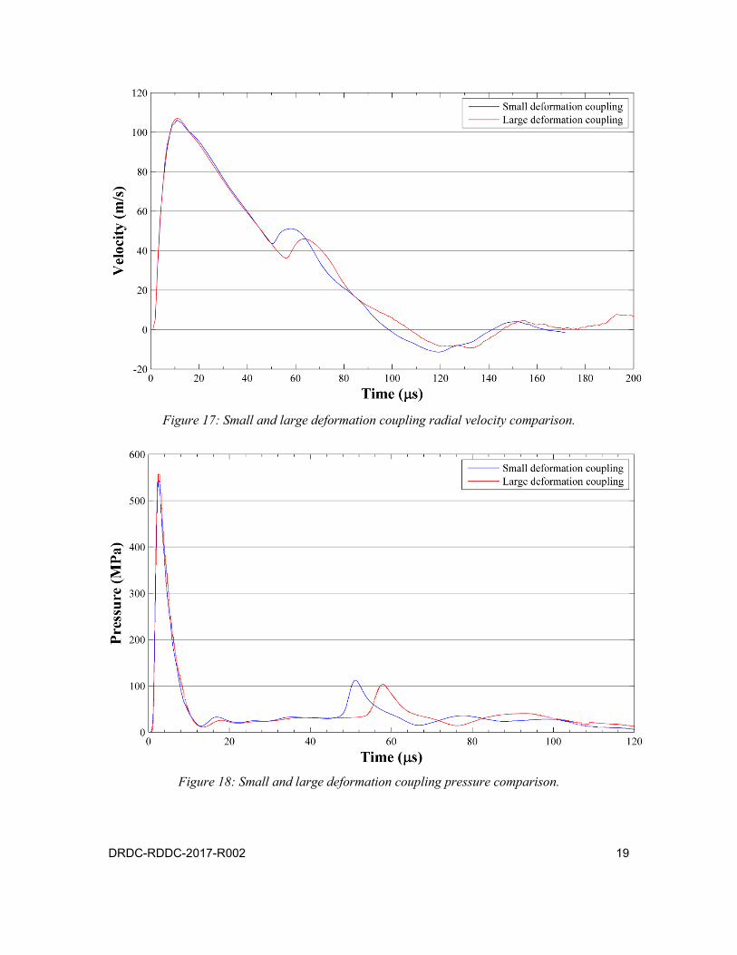
(~60 μs). For the large deformation case, the reloading occurs slightly later; in part because the shockwave from cavitation closure had a larger distance to travel to reach the cylinder wall (deformed shape of the structure is accounted for). The delayed pressure pulse due to cavitation reloading is also evident in Figure 18, where the pressure time-histories for the two cases are shown. The impulse per unit area between 0 μs and 120 μs was determined by trapezoidal integration and was greater for the large deformation coupling case than for small deformation coupling. The impulse per unit area at the cylinder mid-height was 5608 MPa·s in the case of large deformation coupling versus 5330 MPa·s in the case of small deformation coupling, representing an increase of 5.2% with large deformation coupling enabled.
Figure 16: Small and large deformation coupling radial displacement comparison.
DRDC-RDDC-2017-R002 19
Figure 17: Small and large deformation coupling radial velocity comparison.
Figure 18: Small and large deformation coupling pressure comparison.
20 DRDC-RDDC-2017-R002
3.5 Axisymmetric Model
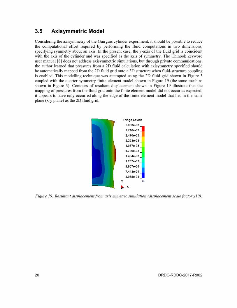
Considering the axisymmetry of the Guirguis cylinder experiment, it should be possible to reduce the computational effort required by performing the fluid computations in two dimensions, specifying symmetry about an axis. In the present case, the y-axis of the fluid grid is coincident with the axis of the cylinder and was specified as the axis of symmetry. The Chinook keyword user manual [8] does not address axisymmetric simulations, but through private communications, the author learned that pressures from a 2D fluid calculation with axisymmetry specified should be automatically mapped from the 2D fluid grid onto a 3D structure when fluid-structure coupling is enabled. This modelling technique was attempted using the 2D fluid grid shown in Figure 3 coupled with the quarter symmetry finite element model shown in Figure 19 (the same mesh as shown in Figure 3). Contours of resultant displacement shown in Figure 19 illustrate that the mapping of pressures from the fluid grid onto the finite element model did not occur as expected; it appears to have only occurred along the edge of the finite element model that lies in the same plane (x-y plane) as the 2D fluid grid.
Figure 19: Resultant displacement from axisymmetric simulation (displacement scale factor x10).
DRDC-RDDC-2017-R002 21
4 Conclusion
A Guirguis hydro-bulged cylinder experiment was simulated using the Chinook hydrocode coupled with the LS-DYNA explicit dynamics solver. The objective was to validate the simulation methodology and to investigate how different modelling parameters and options would affect the accuracy of the results. The following summarizes the conclusions drawn from the study:
The coupled Chinook hydrocode and the LS-Dyna explicit dynamics solver are capableof predicting primary load and response characteristics observed in close-proximityUNDEX experiments including
o initial interaction between the shockwave generated by detonation of theexplosive and the wetted surface of the structure;
o reflection of the shockwave off of the structure surface;
o subsequent reflection of the reflected wave off of the gas bubble surface as ararefaction wave;
o cavitation between the gas bubble and the structure resulting from pressurecut-off near the fluid-structure interface combined with the aforementionedreflected rarefaction wave; and
o closure of the cavitated region of fluid and reloading of the structure by the shockpulse produced by cavitation closure.
For a given explosive, there may be a wide range of JWL equation of state parametersavailable in literature. The choice of parameters can have a significant influence onsimulations results. In the case studied here, the difference in maximum deformationpredicted using different sets of EOS parameters was approximately 14%. The reason forthe difference in parameters in the present case is unknown, but it may be related to theexplosive composition (i.e. inclusion of inert binders or aluminum), the method ofexplosive manufacture, or the type of test that was used to derive the EOS parameters.Thus, it is recommended that explosive compositions with known properties be used inexperiments and that experiment reports include as much information as possible on theexplosive so that suitable properties for use in simulations can be determined.Furthermore, the influence of explosive properties on simulation results highlights theneed to use accurate properties for explosives found in naval weapons so that simulationsof full-scale UNDEX in close-proximity to naval platforms can be carried out withconfidence.
The element formulation used in the structural model can significantly influencesimulation results. Although hexahedral elements performed well, shell elements arepreferred for modelling of marine structures due to their computational efficiency. Thedefault shell element formulation (Belytschko-Tsay) used in LS-DYNA resulted in anunder-prediction of the cylinder deformation when compared with a simulation using the
22 DRDC-RDDC-2017-R002
Hughes-Liu formulation. The Hughes-Liu formulation gave results in best agreement with experimental measurements, under-predicting the maximum mid-height radial deformation by 5.44%, compared to 9.82% using the Belytschko-Tsay formulation and 6.49% using hexahedrons. The improved accuracy attained using Hughes-Liu element is attributed to its formulation accounting for situations where an elements nodes do not all lie in the same plane, as was the case for the cylinder model. This element formulation should be considered for future use in modelling ship and submarine structures that have curved surfaces and that can undergo large deformations causing nodes to become non-planar (twisting of hull plating, stiffeners, etc.) when subjected to loads from underwater explosions. It should be noted that this element formulation is more computationally expensive than the default Belytschko-Tsay formulation and the small potential increase in accuracy should be weighed against decreased computational performance.
In cases where rapid deformation of the structure occurs along with a reduction of fluidpressure at the fluid-structure interface, using a large deformation coupling algorithm thatadjusts the fluid grid so that it follows the deformed structure can have a markedinfluence on results. In simulations of the cylinder experiment, large deformationcoupling increased the impulse imparted to a point on the cylinder at its mid-height byapproximately 5%. The difference in impulse may not be as large for other charge sizesand/or standoff distances. The potential benefit should be weighed against the increase incalculation time that results from invoking large deformation coupling.
Axisymmetry can be taken advantage of to significantly reduce simulation time inappropriate cases. However, the Chinook hydrocode does not appear to properly executemapping of pressures from a two-dimensional axisymmetric fluid grid to athree-dimensional structure. It is possible that the erroneous result that was obtained wasdue to errors in user implementation. If that is the case, the Chinook user manual shouldbe updated to better explain the process of running an axisymmetric fluid-structureinteraction simulation.
The Chinook hydrocode coupled with the LS-DYNA explicit dynamics solver simulated the early stages of Guirguis hydro-bulged cylinder experiment with acceptable accuracy. A particular combination of JWL parameters ([16]), element formulation (Hughes-Liu) and fluid-structure coupling predicted the maximum mid-height deformation within 5.44% of the measured value. In future simulations of close-proximity UNDEX, care should be taken to ensure accurate explosive properties are used in the JWL equation of state model. Also, structural models made up of shell elements may be used for full-scale models of naval platforms with the knowledge that they will provide an accurate representation of the structure compared with solid elements. The shell element formulation that is used should allow for large deformations and account for non-planar node locations, both initially and as the elements deform with node locations being updated during the solution.
The largest shortcoming of the simulation methodology is that simulations sometimes fail prematurely with a ‘not a number’ or ‘negative sound speed in JWL EOS’ error generated by the Chinook code. Developers have explained that this is likely due to failure of the iterative algorithm in the Chinook code that calculates state variables in cells with mixed materials where the equations of state have different forms e.g. water (Tait or Tillotson EOS) and explosive
DRDC-RDDC-2017-R002 23
products (JWL EOS). This occurrence of this error is unpredictable; it occurred when different fluid grids and EOS parameters were used. Changing EOS parameters allowed some simulations to run longer than others, but the end result was most often premature termination. In simulations unrelated to this report, changing the tolerance in the *MULTIMATERIAL CONTROL keyword of the Chinook input file was sometimes sufficient to overcome premature termination. Unfortunately, there is no known reliable way to overcome this error in the current version of the Chinook code and a trial-and-error approach to changing the fluid grid and/or adjusting the *MULTIMATERIAL CONTROL keyword is sometimes unavoidable. Means of overcoming these issues are being considered for implementation in future versions of the Chinook hydrocode. The first would be to devise a general equation of state that has a form suitable for use with multiple materials so that state variables in cells with mixed materials may be solved for in a deterministic way rather than an iterative one. Another option might be to switch the JWL material to an ideal gas once the pressure in the explosive products has fallen sufficiently since the JWL EOS limits to the ideal gas equation at low pressure. For example, for the explosive cyclotrimethylenetrinitramine also known as research department formula x (RDX), there is little difference in the volume versus pressure relationship at pressures below 400 MPa [19].

24 DRDC-RDDC-2017-R002
This page intentionally left blank.
25 DRDC-RDDC-2017-R002
5 References
[1] Army Materiel Command Alexandra VA (1974), Engineering design handbook. Explosions in air. Part one. Accession number ADA003817, Army Materiel Command, Alexandria, VA.
[2] Cole RH (1948), Underwater explosions. Princeton NJ: Princeton University Press.
[3] Wardlaw A, McKeown R and Luton A (1998), Coupled hydrocode prediction of underwater explosion damage, Naval Surface Warfare Center Indian Head Division, Indian Head MD.
[4] Wardlaw A and Luton A (2000), Fluid-structure interaction mechanisms for close-in explosions, Shock and Vibration 7, 265–275.
[5] Sandusky H, Chambers P, Zerilli F, Fabini L and Gottwald W (1999), Dynamic measurements of plastic deformation in a water-filled aluminum tube in response to detonation of a small explosive charge, Shock and Vibration 6, 125–132.
[6] Chambers G, Sandusky H, Zerilli F, Rye K, Tussing R and Forbes J (2001), Pressure measurements on a deforming surface in response to an underwater explosion in a water-filled aluminum tube, Shock and Vibration 8, 1–7.
[7] IABG (1995), Dynamic systems mechanics advanced simulation coupled Eulerian-Lagrangian hydrocode, Ottobrunn Germany.
[8] Lloyd’s Register Applied Technology Group (2016), ChinookEXP input manual, Martec software manual #SM-13-04 Rev 17 ChinookEXP v210, Halifax NS.
[9] LSTC (2012), LS-DYNA keyword user’s manual, Volume 1 Livermore Software Technology Corporation (LSTC), Version 971 R6.1.0, Livermore CA.
[10] Pointwise Inc. (2012), Pointwise user manual, Version 17.0 Release 2, Fort Worth, TX.
[11] Li Yuan-Hui (1967). Equation of state of water and sea water. Journal of Geophysical research, 17(10), 2665, May 1967.
[12] Tillotson JH (1962), Metallic equations of state for hypervelocity impact. General Atomic report GA-3216, General Atomic, San Diego, CA.
[13] Baudin G and Serradeill R (2010), Review of Jones-Wilkins-Lee equation of state. EPJ Web of Conferences 10, 00021 (2010), EDP Sciences, London.
[14] Chopra AK (1995), Dynamics of structures: theory and applications to earthquake engineering, Prentice Hall, New Jersey, NJ.
[15] Dobratz BM and Crawford PC (1985), LLNL Explosives Handbook: properties of chemical explosives and explosive simulants, Lawrence Livermore National Laboratory, University of California.
DRDC-RDDC-2017-R002 26
[16] Tao WC, Tarver CM, Kury JW, Lee CG and Ornellas DL (1993), Understanding composite explosive energetics: IV. Reactive flow modeling of aluminum reaction kinetics in PETN and TNT using normalized product equation of state, Tenth International Detonation Symposium, Boston, MA, July 12–16 1993.
[17] McGlaun JM, Thompson SL and Elrick MG (1990), CTH: A three-dimensional shock wave physics code, Int. J. Impact Eng. 10, pp. 351–360.
[18] Brundage A (2014), Prediction of shock-induced cavitation in water, Journal of Physics: Conference Series 500, Part 10, 1–4.
[19] Amar S, Kochavi E, Lefler Y, Vaintraub S and Sidilkover D (2015), Comparison of BKW and JWL equations of state for explosive simulations, The 30th International Symposium on Shock Waves - ISSW30, Vol 2, Chapter 39, Tel-Aviv, Israel.
DRDC-RDDC-2017-R002 27
List of symbols/abbreviations/acronyms/initialisms
2D Two-dimensional
3D Three-dimensional
A JWL EOS parameter (Pa), Tillotson EOS parameter
B JWL EOS parameter (Pa), Tait EOS parameter, Zerilli-Armstrong material parameter
c Speed of sound
C Tillotson EOS parameter
C0 Zerilli-Armstrong material model yield strength
eint Internal energy
eint,0 Reference internal energy
g Grams
m Tait EOS parameter
n Tait EOS parameter
p Pressure
p0 Reference pressure
β0 Zerilli-Armstrong material model parameter
β1 Zerilli-Armstrong material model parameter
μ Tillotson EOS variable
ρ Density
ρ0 Reference density
ω JWL EOS parameter (constant)
γ Ideal gas EOS polytropic index
CFD Computational fluid dynamics
DRDC Defence Research and Development Canada
ELFORM Element form
EOS Equation of state
FE Finite element
FEA Finite element analysis
JWL Jones-Wilkins-Lee
O.D. Outside diameter

28 DRDC-RDDC-2017-R002
PETN Pentaerythritol tetranitrate
RDX Research department formula X
R1 JWL EOS parameter (constant)
R2 JWL EOS parameter (constant)
UNDEX Underwater explosion

DOCUMENT CONTROL DATA (Security markings for the title, abstract and indexing annotation must be entered when the document is Classified or Designated)
1. ORIGINATOR (The name and address of the organization preparing the document.Organizations for whom the document was prepared, e.g. Centre sponsoring a contractor's report, or tasking agency, are entered in section 8.)
Defence Research and Development Canada –Atlantic Research Centre9 Grove StreetP.O. Box 1012Dartmouth, Nova Scotia B2Y 3Z7
2a. SECURITY MARKING (Overall security marking of the document including special supplemental markings if applicable.)
UNCLASSIFIED
2b. CONTROLLED GOODS
(NON-CONTROLLED GOODS) DMC A REVIEW: GCEC DEC 2013
3. TITLE (The complete document title as indicated on the title page. Its classification should be indicated by the appropriate abbreviation (S, C or U) in parentheses after the title.)
Simulation of the Guirguis cylinder experiment using coupled Chinook/LS-DYNA
4. AUTHORS (last name, followed by initials – ranks, titles, etc. not to be used)
Liam Gannon
5. DATE OF PUBLICATION(Month and year of publication of document.)
January 2017
6a. NO. OF PAGES (Total containing information, including Annexes, Appendices, etc.)
40
6b. NO. OF REFS (Total cited in document.)
19 7. DESCRIPTIVE NOTES (The category of the document, e.g. technical report, technical note or memorandum. If appropriate, enter the type of report,
e.g. interim, progress, summary, annual or final. Give the inclusive dates when a specific reporting period is covered.)
Scientific Report
8. SPONSORING ACTIVITY (The name of the department project office or laboratory sponsoring the research and development – include address.)
Defence Research and Development Canada – Atlantic Research Centre9 Grove StreetP.O. Box 1012Dartmouth, Nova Scotia B2Y 3Z7
9a. PROJECT OR GRANT NO. (If appropriate, the applicable research and development project or grant number under which the document was written. Please specify whether project or grant.)
01EA
9b. CONTRACT NO. (If appropriate, the applicable number under which the document was written.)
10a. ORIGINATOR'S DOCUMENT NUMBER (The official document number by which the document is identified by the originating activity. This number must be unique to this document.)
DRDC-RDDC-2017-R002
10b. OTHER DOCUMENT NO(s). (Any other numbers which may be assigned this document either by the originator or by the sponsor.)
11. DOCUMENT AVAILABILITY (Any limitations on further dissemination of the document, other than those imposed by security classification.)
Unlimited
12. DOCUMENT ANNOUNCEMENT (Any limitation to the bibliographic announcement of this document. This will normally correspond to theDocument Availability (11). However, where further distribution (beyond the audience specified in (11) is possible, a wider announcement audience may be selected.))
Unlimited
13. ABSTRACT (A brief and factual summary of the document. It may also appear elsewhere in the body of the document itself. It is highly desirable that the abstract of classified documents be unclassified. Each paragraph of the abstract shall begin with an indication of the security classification of the information in the paragraph (unless the document itself is unclassified) represented as (S), (C), (R), or (U). It is not necessary to include here abstracts in both official languages unless the text is bilingual.)
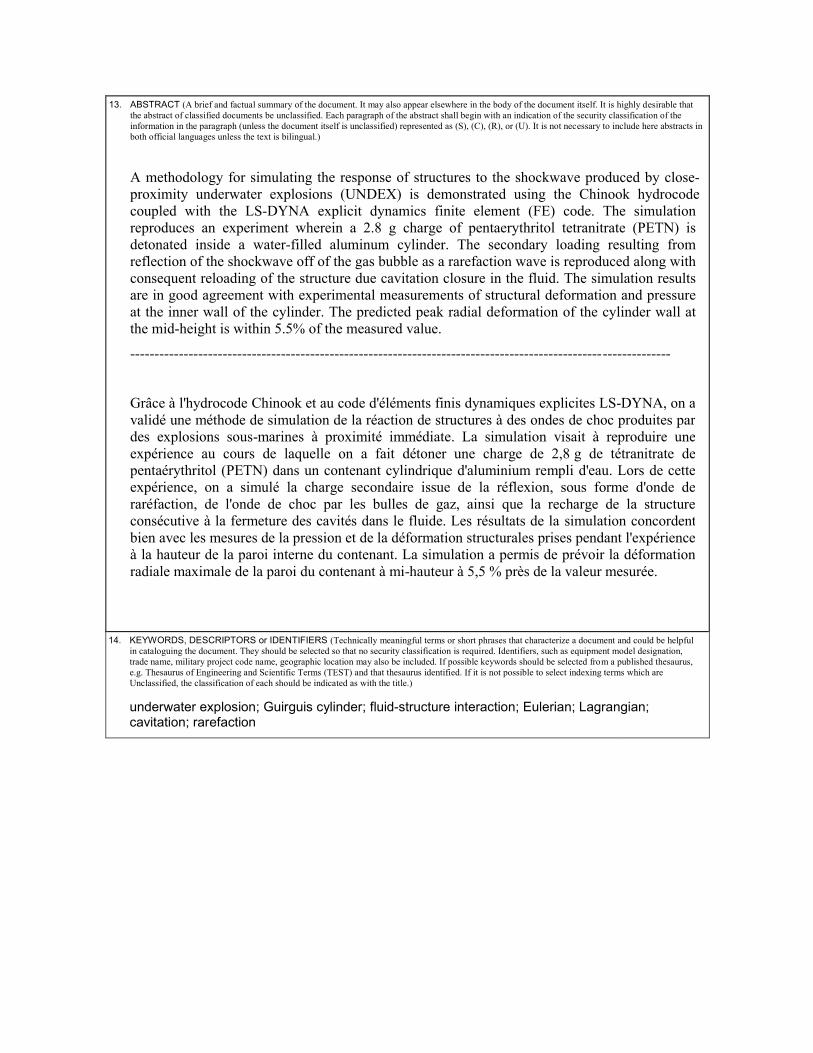
A methodology for simulating the response of structures to the shockwave produced by close-proximity underwater explosions (UNDEX) is demonstrated using the Chinook hydrocode coupled with the LS-DYNA explicit dynamics finite element (FE) code. The simulation reproduces an experiment wherein a 2.8 g charge of pentaerythritol tetranitrate (PETN) is detonated inside a water-filled aluminum cylinder. The secondary loading resulting from reflection of the shockwave off of the gas bubble as a rarefaction wave is reproduced along with consequent reloading of the structure due cavitation closure in the fluid. The simulation results are in good agreement with experimental measurements of structural deformation and pressure at the inner wall of the cylinder. The predicted peak radial deformation of the cylinder wall at the mid-height is within 5.5% of the measured value.
---------------------------------------------------------------------------------------------------------------
Grâce à l'hydrocode Chinook et au code d'éléments finis dynamiques explicites LS-DYNA, on a validé une méthode de simulation de la réaction de structures à des ondes de choc produites par des explosions sous-marines à proximité immédiate. La simulation visait à reproduire une expérience au cours de laquelle on a fait détoner une charge de 2,8 g de tétranitrate de pentaérythritol (PETN) dans un contenant cylindrique d'aluminium rempli d'eau. Lors de cette expérience, on a simulé la charge secondaire issue de la réflexion, sous forme d'onde de raréfaction, de l'onde de choc par les bulles de gaz, ainsi que la recharge de la structure consécutive à la fermeture des cavités dans le fluide. Les résultats de la simulation concordent bien avec les mesures de la pression et de la déformation structurales prises pendant l'expérience à la hauteur de la paroi interne du contenant. La simulation a permis de prévoir la déformation radiale maximale de la paroi du contenant à mi-hauteur à 5,5 % près de la valeur mesurée.
14. KEYWORDS, DESCRIPTORS or IDENTIFIERS (Technically meaningful terms or short phrases that characterize a document and could be helpful in cataloguing the document. They should be selected so that no security classification is required. Identifiers, such as equipment model designation, trade name, military project code name, geographic location may also be included. If possible keywords should be selected from a published thesaurus, e.g. Thesaurus of Engineering and Scientific Terms (TEST) and that thesaurus identified. If it is not possible to select indexing terms which are Unclassified, the classification of each should be indicated as with the title.)
underwater explosion; Guirguis cylinder; fluid-structure interaction; Eulerian; Lagrangian; cavitation; rarefaction