simulation of manufacturing systems -...
TRANSCRIPT

14-1
C H A P T E R 1 4
Simulation of
Manufacturing Systems
Recommended sections for a fi rst reading: 14.1, 14.2, 14.4, 14.5
14.1 INTRODUCTION
There continues to be widespread use of simulation to design and “optimize” manu-facturing systems. As a matter of fact, it could arguably be said that simulation is more widely applied to manufacturing systems than to any other application area. Some reasons for this include the following:
• Increased competition in many industries has resulted in greater emphasis on automation to improve productivity and quality. Since automated systems are more complex, they typically can only be analyzed by simulation.
• The cost of equipment and facilities can be quite large. For example, a new semi-conductor manufacturing plant can cost a billion dollars or even more.
• The cost of computing has decreased dramatically as a result of faster and cheaper PCs.
• Improvements in simulation software (e.g., graphical user interfaces) have reduced model-development time, thereby allowing for more timely manufacturing analyses.
• The availability of animation has resulted in greater understanding and use of simulation by manufacturing managers.
The remainder of this chapter is organized as follows. In Sec. 14.2 we discuss the types of manufacturing issues typically addressed by simulation. Section 14.3 gives brief descriptions of FlexSim and ProModel, which are popular manufacturing-oriented simulation packages. A simulation model of the small factory considered
Law01323_ch14_001-047.indd Page 14-1 23/10/13 4:31 PM user-f-w-198 Law01323_ch14_001-047.indd Page 14-1 23/10/13 4:31 PM user-f-w-198 /203/MH02090/Law01323_disk1of1/0073401323/Law01323_pagefiles/203/MH02090/Law01323_disk1of1/0073401323/Law01323_pagefiles

14-2 simulation of manufacturing systems
in Chap. 3 is also given for each package. Modeling of manufacturing-system randomness, including machine downtimes, is discussed in Sec. 14.4. Sections 14.5 and 14.6 show in considerable detail how simulation is actually used to design and analyze a manufacturing system.
A good reference on manufacturing systems in general is Hopp and Spearman (2011). Many actual applications of simulation in manufacturing can be found in the Proceedings of the Winter Simulation Conference, which is published every December (see www.wintersim.org).
14.2 OBJECTIVES OF SIMULATION IN MANUFACTURING
Perhaps the greatest overall benefi t of using simulation in a manufacturing environ-ment is that it allows a manager or an engineer to obtain a systemwide view of the effect of “local” changes to the manufacturing system. If a change is made at a particular workstation, its impact on the performance of this station may be predict-able. On the other hand, it may be diffi cult, if not impossible, to determine ahead of time the impact of this change on the performance of the overall system.
E X A M P L E 1 4 . 1 . Suppose that a workstation with one machine has insuffi cient process-ing capacity to handle its workload (i.e., its processing rate is less than the arrival rate of parts). Suppose further that it has been determined that adding a second machine will alleviate the capacity shortage at this station. However, this additional machine will also increase the throughput of parts from this station. This increased throughput will, in turn, show up as increased arrival rates to downstream workstations, which may cause new capacity shortages to occur, etc.
In addition to the above general benefi t of simulation, there are a number of specifi c potential benefi ts from using simulation for manufacturing analyses, including:
• Increased throughput (parts produced per unit of time)• Decreased times in system of parts• Reduced in-process inventories of parts• Increased utilizations of machines or workers• Increased on-time deliveries of products to customers• Reduced capital requirements (land, buildings, machines, etc.) or operating
expenses• Insurance that a proposed system design will, in fact, operate as expected• Information gathered to build the simulation model will promote a greater under-
standing of the system, which often produces other benefi ts.• A simulation model for a proposed system often causes system designers to
think about certain signifi cant issues (e.g., system control logic) long before they normally would.
E X A M P L E 1 4 . 2 . The information gathered for a simulation model of a food-packing plant showed that the control logic for the conveyor system was not implemented correctly.
Law01323_ch14_001-047.indd Page 14-2 06/11/13 9:29 PM user-f-w-198 Law01323_ch14_001-047.indd Page 14-2 06/11/13 9:29 PM user-f-w-198 /203/MH02090/Law01323_disk1of1/0073401323/Law01323_pagefiles/203/MH02090/Law01323_disk1of1/0073401323/Law01323_pagefiles

chapter fourteen 14-3
Simulation has successfully addressed a number of particular manufacturing issues, which we might classify into three general categories:
The need for and the quantity of equipment and personnel
• Number, type, and layout of machines for a particular objective (e.g., production of 1000 parts per week)
• Requirements for material-handling systems and other support equipment (e.g., pallets and fi xtures)
• Location and size of inventory buffers• Evaluation of a change in product volume or mix (e.g., impact of new products)• Evaluation of the effect of a new piece of equipment (e.g., a robot) on an existing
manufacturing line• Evaluation of capital investments• Labor-requirements planning• Number of shifts
Performance evaluation
• Throughput analysis• Time-in-system analysis• Bottleneck analysis [i.e., determining the location of the constraining resource(s)]
Evaluation of operational procedures
• Production scheduling (i.e., evaluating proposed policies for dispatching orders to the shop fl oor, choosing batch sizes, loading parts at a workstation, and sequenc-ing of parts through the workstations in the system)
• Policies for component-part or raw-material inventory levels• Control strategies [e.g., for a conveyor system or an automated guided vehicle
system (AGVS)]• Reliability analysis (e.g., effect of preventive maintenance)• Quality-control policies (e.g., Six Sigma)• Just-in-time (JIT) strategies
There are several common measures of performance obtained from a simula-tion study of a manufacturing system, including:
• Throughput• Time in system for parts (cycle time)• Times parts spend in queues• Times parts spend waiting for transport• Times parts spend in transport• Timeliness of deliveries (e.g., proportion of late orders)• Sizes of in-process inventories (work-in-process or queue sizes)• Utilization of equipment and personnel (i.e., proportion of time busy)• Proportions of time that a machine is broken, starved (waiting for parts from a
previous workstation), blocked (waiting for a fi nished part to be removed), or undergoing preventive maintenance
• Proportions of parts that are reworked or scrapped
Law01323_ch14_001-047.indd Page 14-3 23/10/13 4:31 PM user-f-w-198 Law01323_ch14_001-047.indd Page 14-3 23/10/13 4:31 PM user-f-w-198 /203/MH02090/Law01323_disk1of1/0073401323/Law01323_pagefiles/203/MH02090/Law01323_disk1of1/0073401323/Law01323_pagefiles

14-4 simulation of manufacturing systems
14.3 SIMULATION SOFTWARE FOR MANUFACTURING APPLICATIONS
The simulation-software requirements for manufacturing applications are not fun-damentally different from those for other simulation applications, with one excep-tion. Most modern manufacturing facilities contain material-handling systems, which are often diffi cult to model correctly. Therefore, in addition to the software features discussed in Chap. 3, it is desirable for simulation packages used in manu-facturing to have fl exible, easy-to-use material-handling modules. Important classes of material-handling systems are forklift trucks, AGVS with contention for guide paths, transport conveyors (equal distance between parts), accumulating (or queueing) conveyors, power-and-free conveyors, automated storage-and-retrieval systems (AS/RS), bridge cranes, and robots. Note that just because a particular software package contains conveyor constructs doesn’t necessarily mean that they are ap-propriate for a given application. Indeed, real-world conveyor systems come in a wide variety of forms, and different software packages have varying degrees of conveyor capabilities.
In Chap. 3 we defi ned general-purpose and application-oriented simulation packages, and then we discussed three general-purpose packages in some detail. General-purpose packages usually offer considerable modeling fl exibility and are widely used to simulate manufacturing systems. Furthermore, some of these products (e.g., Arena and ExtendSim) provide modeling constructs (e.g., conveyors) specifi cally for manufacturing. There are also many simulation packages designed specifi cally for use in a manufacturing environment. In Secs. 14.3.1 and 14.3.2 we give descriptions of FlexSim and ProModel, respectively, which are, at the time of this writing, two popular manufacturing-oriented simulation packages. In each case, we also show how to build a model of the small factory considered in Sec. 3.5. Section 14.3.3 lists some additional manufacturing-oriented simulation packages.
14.3.1 FlexSim
FlexSim [see Beaverstock et al. (2013) and FlexSim (2013)] is a true object-oriented simulation package for manufacturing, material handling, warehousing, and fl ow processes marketed by FlexSim Software Products (Orem, Utah). A model is constructed by dragging and dropping “objects” into the “Model View” and then editing their parameters using dialog boxes. FlexSim can model a wide variety of manufacturing confi gurations, since existing objects can be fully cus-tomized to meet specifi c requirements. These customized objects can then be placed in the library for reuse in current or future modeling applications. A model can also have an unlimited number of levels of hierarchy and use all aspects of object-oriented technology (i.e., encapsulation, inheritance, and polymorphism, as discussed in Sec. 3.6).
Law01323_ch14_001-047.indd Page 14-4 23/10/13 4:31 PM user-f-w-198 Law01323_ch14_001-047.indd Page 14-4 23/10/13 4:31 PM user-f-w-198 /203/MH02090/Law01323_disk1of1/0073401323/Law01323_pagefiles/203/MH02090/Law01323_disk1of1/0073401323/Law01323_pagefiles

chapter fourteen 14-5
FlexSim provides three-dimensional, prospective-projection model building and animation by default; however, the user has the option to switch to an ortho-graphic view or display both views simultaneously.
Material-handling devices available in FlexSim include conveyors (transport and accumulating), forklift trucks, AGVS, AS/RS, cranes, elevators, robots, and operators. FlexSim provides preempting and priority processing for capturing de-tails of product movement and processing.
The FlexSim software includes a cost model that allows one to account for the profi t for each part produced and also for the costs associated with machines, labor, work-in-process, etc.
There are an unlimited number of random-number streams available in FlexSim. Furthermore, the user has access to 24 standard theoretical probability distributions and also to empirical distributions. The time to failure of a machine can be based on busy time, calendar time, or a user-defi ned event.
There is an “Experimenter” that can be used to automatically make independent replications for each of a number of different scenarios, and to obtain point esti-mates and confi dence intervals for performance measures of interest. Furthermore, the replications can be simultaneously executed across multiple processor cores. A number of plots are available, including time plots, histograms, bar charts, pie charts, and Gantt charts.
The ExpertFit distribution-fi tting software (see Sec. 6.7) is bundled with FlexSim, while the OptQuest “optimization” module (see Sec. 12.5.2) is available as an op-tion. FlexSim Software Products also develops and markets the FlexSim Healthcare simulation package.
The FlexSim model of the manufacturing system consists of the six objects shown in Fig. 14.1, which is the orthographic view of the model. The dialog box
FIGURE 14.1FlexSim model for the manufacturing system, as shown in the orthographic view.
Law01323_ch14_001-047.indd Page 14-5 23/10/13 4:31 PM user-f-w-198 Law01323_ch14_001-047.indd Page 14-5 23/10/13 4:31 PM user-f-w-198 /203/MH02090/Law01323_disk1of1/0073401323/Law01323_pagefiles/203/MH02090/Law01323_disk1of1/0073401323/Law01323_pagefiles

14-6 simulation of manufacturing systems
for the “Source” object named “PartsArrive” (the left-most object in Figure 14.1) is shown in Fig. 14.2; here we specify that the interarrival times of parts (called “fl owitems” in FlexSim) are exponentially distributed with a mean of 1 (and a loca-tion parameter of 0) and use random-number stream 1 (see Chap. 7). (The time unit for the simulation model is set to minutes at the beginning of the model-building process.) The statistical-distribution dialog box displays a histogram of 1000 gener-ated interarrival times.
The next object is a “Queue” object named “MachineQ,” whose dialog box is shown in Fig. 14.3. The dialog box for the “Processor” object named “Machine” is
FIGURE 14.2Dialog box for the FlexSim Source object “PartsArrive.”
Law01323_ch14_001-047.indd Page 14-6 23/10/13 4:31 PM user-f-w-198 Law01323_ch14_001-047.indd Page 14-6 23/10/13 4:31 PM user-f-w-198 /203/MH02090/Law01323_disk1of1/0073401323/Law01323_pagefiles/203/MH02090/Law01323_disk1of1/0073401323/Law01323_pagefiles

chapter fourteen 14-7
shown in Fig. 14.4, where we specify that processing times are uniformly distributed with a minimum value of 0.65 and a maximum value of 0.70, and we use random-number stream 2.
The dialog box for the Queue object named “InspectorQ” is similar to that for the MachineQ object and is not shown. The dialog box for the Processor
FIGURE 14.3Dialog box for the FlexSim Queue object “MachineQ.”
Law01323_ch14_001-047.indd Page 14-7 23/10/13 4:31 PM user-f-w-198 Law01323_ch14_001-047.indd Page 14-7 23/10/13 4:31 PM user-f-w-198 /203/MH02090/Law01323_disk1of1/0073401323/Law01323_pagefiles/203/MH02090/Law01323_disk1of1/0073401323/Law01323_pagefiles

14-8 simulation of manufacturing systems
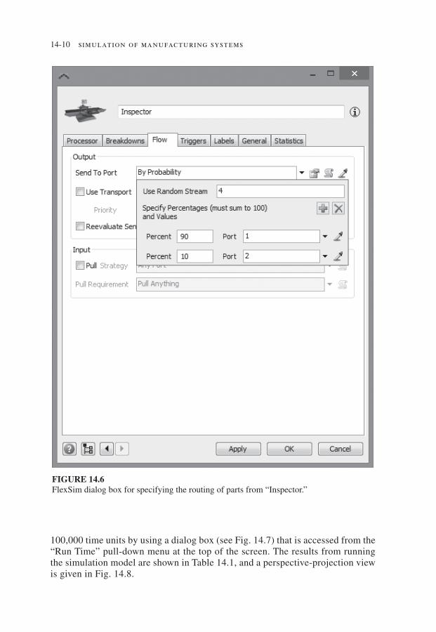
object named “Inspector,” which is similar to that for the Machine object, is shown in Fig. 14.5. Here we specify that inspection times are uniformly distrib-uted with a minimum value of 0.75 and a maximum value of 0.80, and we use random-number stream 3. Also, if we click on the “Flow” tab near the top of the screen, we can access the dialog box shown in Fig. 14.6. Here we specify that
FIGURE 14.4Dialog box for the FlexSim Processor object “Machine.”
Law01323_ch14_001-047.indd Page 14-8 23/10/13 4:31 PM user-f-w-198 Law01323_ch14_001-047.indd Page 14-8 23/10/13 4:31 PM user-f-w-198 /203/MH02090/Law01323_disk1of1/0073401323/Law01323_pagefiles/203/MH02090/Law01323_disk1of1/0073401323/Law01323_pagefiles

chapter fourteen 14-9
90 percent of the fl owitems (i.e., those that are good) go to output port 1 (using random-number stream 4), which is connected to the “Sink” object named “PartsDepart” (its dialog box is not shown). The remaining 10 percent of the parts (i.e., those that are bad) go to output port 2, where they are sent back to the MachineQ object to be reworked. The simulation run length is specifi ed to be
FIGURE 14.5Dialog box for the FlexSim Processor object “Inspector.”
Law01323_ch14_001-047.indd Page 14-9 23/10/13 4:31 PM user-f-w-198 Law01323_ch14_001-047.indd Page 14-9 23/10/13 4:31 PM user-f-w-198 /203/MH02090/Law01323_disk1of1/0073401323/Law01323_pagefiles/203/MH02090/Law01323_disk1of1/0073401323/Law01323_pagefiles
14-10 simulation of manufacturing systems
100,000 time units by using a dialog box (see Fig. 14.7) that is accessed from the “Run Time” pull-down menu at the top of the screen. The results from running the simulation model are shown in Table 14.1, and a perspective-projection view is given in Fig. 14.8.
FIGURE 14.6FlexSim dialog box for specifying the routing of parts from “Inspector.”
Law01323_ch14_001-047.indd Page 14-10 23/10/13 4:31 PM user-f-w-198 Law01323_ch14_001-047.indd Page 14-10 23/10/13 4:31 PM user-f-w-198 /203/MH02090/Law01323_disk1of1/0073401323/Law01323_pagefiles/203/MH02090/Law01323_disk1of1/0073401323/Law01323_pagefiles

chapter fourteen 14-11
FIGURE 14.7FlexSim dialog box for specifying the simulation run length.
TABLE 14.1
Simulation results for the FlexSim model of the manufacturing system
Output statistic Observed value
Average time in system 4.42Machine utilization 0.75Inspector utilization 0.86Average delay in machine queue 1.01Average number in machine queue 1.12Average delay in inspector queue 1.52Average number in inspector queue 1.68
14.3.2 ProModel
ProModel [see Harrell et al. (2012) and ProModel (2013)] is a manufacturing-oriented simulation package developed and marketed by ProModel Corporation (Orem, Utah). The following are some of the basic modeling constructs, the fi rst four of which must be in every model:
Locations Used to model machines, queues, conveyors, or tanks (see below)
Entities Used to represent parts, raw materials, or information
Arrivals Used to specify how parts enter the system
Processes Used to defi ne the routing of parts through the system and to specify what operations are performed for each part at each location
Resources Used to model static or dynamic resources such as workers or forklift trucks
A model can be constructed graphically (e.g., routings for parts can be defi ned by clicking on graphical locations), by fi lling in data fi elds, and by “programming” with an internal pseudo-language. It is also possible to call external subroutines written in, say, C or C++. Customized front- and back-end interfaces can be developed using ProModel’s ActiveX capability. For example, an Excel interface can easily be set up for creating or modifying models. ProModel provides two-dimensional anima-tion, which is created automatically when the model is developed. Three-dimensional animation is available using ProModel’s 3D Animator.
Law01323_ch14_001-047.indd Page 14-11 23/10/13 4:31 PM user-f-w-198 Law01323_ch14_001-047.indd Page 14-11 23/10/13 4:31 PM user-f-w-198 /203/MH02090/Law01323_disk1of1/0073401323/Law01323_pagefiles/203/MH02090/Law01323_disk1of1/0073401323/Law01323_pagefiles

14-12 simulation of manufacturing systems
Material-handling capabilities in ProModel include manual handling, trans-port conveyors, accumulating conveyors, forklift trucks, AGVS, and bridge cranes. ProModel also has a tank construct for modeling continuous-fl ow systems. ProModel includes a costing feature that allows one to assign costs to locations, resources, and entities that are then tracked over time.
There are 100 different random-number streams available in ProModel. Further-more, the user has access to 15 standard theoretical probability distributions and also to empirical distributions. The time to failure of a machine may be based on busy time, calendar time, the number of completed parts, or a signal from another part of the model.
There is a “Scenario Manager” that can be used to automatically make indepen-dent replications for each of a number of different scenarios. The results from the simulation runs are displayed in ProModel’s “Output Viewer” in the form of tables and graphs, including state graphs (e.g., whether a machine is busy, idle, down, etc.), time plots, histograms, and pie charts. Point estimates and confi dence inter-vals for performance measures of interest can also be displayed. Custom reports can be created that display a specifi c set of tables and graphs.
In addition to providing the ability to export data to Excel, ProModel also links and integrates with Minitab to provide users with a Six Sigma analysis capability. For each scenario of interest, two charts are automatically generated in Minitab for each Six Sigma metric, namely, the Capability Analysis Chart and the Capability Sixpack Chart. The SimRunner optimization module is also included with ProModel. ProModel Corporation also develops and markets the MedModel, ServiceModel, and ProcessSimulator (a Microsoft Visio add-in) simulation packages.
FIGURE 14.8FlexSim model for the manufacturing system, as shown in perspective-projection view.
Law01323_ch14_001-047.indd Page 14-12 23/10/13 4:31 PM user-f-w-198 Law01323_ch14_001-047.indd Page 14-12 23/10/13 4:31 PM user-f-w-198 /203/MH02090/Law01323_disk1of1/0073401323/Law01323_pagefiles/203/MH02090/Law01323_disk1of1/0073401323/Law01323_pagefiles

chapter fourteen 14-13
The ProModel model for the manufacturing system uses “Locations,” “Enti-ties,” “Arrivals,” and “Processes” modeling constructs. Locations, which will be used to represent the machine, the inspector, and their queues, are selected from the “Build” drop-down menu, or by selecting the Locations icon on the toolbar. The resulting “Locations Module,” which consists of three windows, is shown in Fig. 14.9. The “Locations Graphics” window is shown in the lower-left portion of the screen, the “Locations Edit” table across the top of the screen, and the “Layout” window in the lower-right portion of the screen. For each desired model location, a location icon is selected from the Locations Graphics window and placed in the Layout window. A new record corresponding to this location is automatically added to the Locations Edit table, whose fi elds (Name, Capacity, etc.) can then be edited in an appropriate way. The Locations Edit table and Layout window for the manu-facturing system are shown in Fig. 14.10. In particular, the fi elds for the “Machine” record in the Edit table are as follows:
Cap. The capacity of the Machine location (i.e., the number of parallel ma-chines) is 1.
Units The number of separate units of this location (each having the same char-acteristics) is 1.
DTs There are no downtimes for this location.
Stats Only “Basic” statistics (i.e., machine utilization and average processing time) will be computed for this location.
Rules The Machine, when available, will pick that part in the queue that has been waiting the longest (i.e., the “Oldest”).
The horizontal rectangles in the Layout window represent the machine and the inspector queues. Below each queue is a counter, which displays the current number of parts in the queue as the model is running.
FIGURE 14.9Locations Module for ProModel.
Law01323_ch14_001-047.indd Page 14-13 06/11/13 9:29 PM user-f-w-198 Law01323_ch14_001-047.indd Page 14-13 06/11/13 9:29 PM user-f-w-198 /203/MH02090/Law01323_disk1of1/0073401323/Law01323_pagefiles/203/MH02090/Law01323_disk1of1/0073401323/Law01323_pagefiles

14-14 simulation of manufacturing systems
Entities, which are used to represent parts in this model, are selected from the Build menu, or by selecting the Entities icon on the toolbar. This results in the dis-play of the “Entities Module,” which consists of an “Entities Graphics” window, an “Entities Edit” table, and the Layout window. An entity is specifi ed graphically by selecting an icon from the Entities Graphics window and then editing the record that automatically appears in the Entities Edit table. The Entities Edit table for this model is shown in Fig. 14.11. The “Speed” of an entity is not relevant for this model.
Arrivals, which are used to specify how entities arrive to the system, are also selected from the Build menu or from the toolbar. This results in the display of the “Arrivals Module,” which consists of an “Arrivals Tools” window, an “Arrivals Edit” table, and the Layout window. To specify the manner in which an entity arrives, select the desired entity (“Part” for this model) from those listed in the Arrivals Tools window, and click in the Layout window on the location at which entities are to arrive (“MachineQ” for our model). The Arrivals Edit table for the model is shown in Fig. 14.12. The “E(1,1)” in the “Frequency” fi eld specifi es that parts have exponentially distributed (denoted “E”) interarrival times with a mean of 1 minute (the default time unit), and that random-number stream 1 is being used (see Chap. 7).
FIGURE 14.10Locations Edit table and Layout window for the ProModel model.
FIGURE 14.11Entities Edit table for the ProModel model.
FIGURE 14.12Arrivals Edit table for the ProModel model.
Law01323_ch14_001-047.indd Page 14-14 23/10/13 4:31 PM user-f-w-198 Law01323_ch14_001-047.indd Page 14-14 23/10/13 4:31 PM user-f-w-198 /203/MH02090/Law01323_disk1of1/0073401323/Law01323_pagefiles/203/MH02090/Law01323_disk1of1/0073401323/Law01323_pagefiles

chapter fourteen 14-15
The “Logic” fi eld could be used to execute certain logic at the instant that each entity arrives (e.g., assigning attribute values to the entity).
Selecting “Processing” from the Build menu (or selecting its icon on the toolbar) displays the “Processing Module,” which consists of the “Process Edit” table, the “Routing Edit” table, the “Process Tools” window, and the Layout window. To specify the routing (processing) of an entity graphically, complete the following steps:
1. Select an entity (Part for our model) from the entity list in the Process Tools window. The record for the location at which the entity arrives (MachineQ for our model) is highlighted in the Process Edit table.
2. Click on this location in the Layout window and a rubber-banding routing line appears starting at this location.
3. Click on the destination (succeeding) location for the entity (Machine for our model).
The Layout window for the simulation model after the routing from MachineQ to Machine has been specifi ed is shown in Fig. 14.13. The corresponding Process Edit table and Routing Edit table are shown in Fig. 14.14. For our model, Part is both the entity arriving to and departing from the MachineQ location. (In a more complicated model, a raw-material entity could arrive to a machine and a completed-part entity could depart from the machine.) After the modeling for MachineQ is completed, the routing from Machine to “InspectorQ” is specifi ed in a similar manner. For the Machine record in the Process Edit table (see Fig. 14.15), we must specify that processing times (see the “Operation” fi eld) are uniformly distributed on the interval [0.65, 0.70] minute, which is denoted by “WAIT U(0.675, 0.025, 2).” (The random-number stream is 2.) The routing from InspectorQ to “Inspector” is then specifi ed in a similar manner.
Finally, we must specify the routing out of the Inspector location, which is a little bit more complicated. The Process Edit table and Routing Edit table for this step are shown in Fig. 14.15. There are two routes out of Inspector. Either parts
FIGURE 14.13Layout window showing the route from “MachineQ” to “Machine” for the ProModel model.
FIGURE 14.14Process Edit table and Routing Edit table with the “MachineQ record” selected for the ProModel model.
Law01323_ch14_001-047.indd Page 14-15 23/10/13 4:31 PM user-f-w-198 Law01323_ch14_001-047.indd Page 14-15 23/10/13 4:31 PM user-f-w-198 /203/MH02090/Law01323_disk1of1/0073401323/Law01323_pagefiles/203/MH02090/Law01323_disk1of1/0073401323/Law01323_pagefiles

14-16 simulation of manufacturing systems
leave the system by specifying “EXIT” as the “Destination” with a probability of 0.9, or parts go back to MachineQ with a probability of 0.1. This probabilistic rout-ing is defi ned by double-clicking on the “Rule” fi eld for each of the routings, select-ing “Probability” in the resulting “Routing Rule” dialog box, and then entering the appropriate probability value (see Fig. 14.16). (Note we have also specifi ed that inspection times are uniformly distributed on the interval [0.75, 0.80] minute and use stream 3.)
We specify that the simulation run length is 100,000 minutes by using the “Options” option (see Fig. 14.17) in the “Simulation” drop-down menu. After the simulation has been run, we can look at the results in the Output Viewer. The “Entity Summary” table (Fig. 14.18) shows that the average time in system for the entities called Part is 4.47 minutes.
FIGURE 14.15Process Edit table and Routing Edit table with the “Inspector record” selected for the ProModel model.
FIGURE 14.16Routing Rule dialog box for the ProModel model.
Law01323_ch14_001-047.indd Page 14-16 23/10/13 4:31 PM user-f-w-198 Law01323_ch14_001-047.indd Page 14-16 23/10/13 4:31 PM user-f-w-198 /203/MH02090/Law01323_disk1of1/0073401323/Law01323_pagefiles/203/MH02090/Law01323_disk1of1/0073401323/Law01323_pagefiles

chapter fourteen 14-17
FIGURE 14.17Simulation Options dialog box for the ProModel model.
FIGURE 14.18Entity Summary table for the ProModel model of the manufacturing system.
14.3.3 Other Manufacturing-Oriented Simulation Packages
There are a number of other well-known, manufacturing-oriented simulation pack-ages, including AutoMod [Banks (2004) and Applied (2013)], Enterprise Dynamics [INCONTROL (2013)], Plant Simulation [Siemens (2013)], and WITNESS [Lanner (2013)].
Law01323_ch14_001-047.indd Page 14-17 23/10/13 4:31 PM user-f-w-198 Law01323_ch14_001-047.indd Page 14-17 23/10/13 4:31 PM user-f-w-198 /203/MH02090/Law01323_disk1of1/0073401323/Law01323_pagefiles/203/MH02090/Law01323_disk1of1/0073401323/Law01323_pagefiles

14-18 simulation of manufacturing systems
14.4 MODELING SYSTEM RANDOMNESS
In Chap. 6 we presented a general discussion of how to choose input probability distributions for simulation models, and those ideas are still relevant here. We now discuss some additional topics related to modeling system randomness that are particularly germane to manufacturing systems, with our major emphasis being the representation of machine downtimes.
14.4.1 Sources of Randomness
We begin with a discussion of common sources of randomness in manufacturing systems. In particular, the following are possible examples of continuous distribu-tions in manufacturing:
• Interarrival times of orders, parts, or raw materials• Processing, assembly, or inspection times• Times to failure of a machine (see Sec. 14.4.2)• Times to repair a machine• Loading and unloading times• Setup times to change a machine over from one part type to another• Rework• Product yields
Note that in some cases the above quantities might be constant. For example, pro-cessing times for an automated machine might not vary appreciably. Also, automo-bile engines might arrive to a fi nal assembly area with constant interarrival times of 1 minute.
There are actually two other common ways in which parts “enter” a manufac-turing system. In some systems (e.g., a subassembly manufacturing line), it is often assumed that there is an unlimited supply of raw parts or materials in front of the line’s fi rst machine. Thus, the rate at which parts enter the system is the effective processing rate of the fi rst machine, i.e., accounting for downtimes, blockage, etc. Jobs or orders may also arrive to a system in accordance with a production schedule, which specifi es the time of arrival, the part type, and the order size for each order. In a simulation model, the production schedule might be read from an external fi le.
Histograms of observed processing (or assembly) times, times to failure, and repair times each tend to have a distinctive shape, and examples of these three types of data are given in Figs. 14.19 through 14.21. Note that the times to failure in Fig. 14.20 have an exponential-like shape, with the mode (most likely value) near zero. However, the exponential distribution itself does not provide a good model for these data; see the discussion in Sec. 14.4.2. Observe also that the other two histo-grams have their mode at a positive value and are skewed to the right (i.e., the right tail is longer).
Discrete distributions seem, in general, to be less common than continuous distri-butions in manufacturing systems. However, two examples of discrete distributions
Law01323_ch14_001-047.indd Page 14-18 23/10/13 4:31 PM user-f-w-198 Law01323_ch14_001-047.indd Page 14-18 23/10/13 4:31 PM user-f-w-198 /203/MH02090/Law01323_disk1of1/0073401323/Law01323_pagefiles/203/MH02090/Law01323_disk1of1/0073401323/Law01323_pagefiles

chapter fourteen 14-19
h(x)0.30
0.25
0.20
0.15
0.10
29.001.00 5.00 9.00 13.00 17.00 21.00 25.00
0.05
0.00 x
FIGURE 14.19Histogram of 52 processing times for an automotive manufacturer.
h(x)0.40
0.35
0.30
0.25
0.20
0.15
0.10
3.50 18.50 33.50 48.50 63.50 78.50 93.50
0.05
0.00 x
FIGURE 14.20Histogram of 1603 times to failure for a household-products manufacturer.
Law01323_ch14_001-047.indd Page 14-19 23/10/13 4:31 PM user-f-w-198 Law01323_ch14_001-047.indd Page 14-19 23/10/13 4:31 PM user-f-w-198 /203/MH02090/Law01323_disk1of1/0073401323/Law01323_pagefiles/203/MH02090/Law01323_disk1of1/0073401323/Law01323_pagefiles

14-20 simulation of manufacturing systems
are the outcome of inspecting a part (say, good or bad), and the size of an order arriving to a factory (the possible values are 1, 2, . . .).
14.4.2 Machine Downtimes
The most important source of randomness for many manufacturing systems is that associated with machine breakdowns or unscheduled downtime. Random down-time results from such events as actual machine failures, part jams, and broken tools. The following example illustrates the importance of modeling machine down-time correctly.
E X A M P L E 1 4 . 3 . A company is going to buy a new machine tool from a vendor who claims that the machine will be down 10 percent of the time. However, the vendor has no data on how long the machine will operate before breaking down or on how long it will take to repair the machine. Some simulation analysts have accounted for random breakdowns by simply reducing the machine processing rate by 10 percent. We will see, however, that this can produce results that are quite inaccurate. Suppose that the single-machine-tool system (see, for example, Example 4.32) will actually operate according to the following assumptions when installed by the purchasing company:
• Jobs arrive with exponential interarrival times with a mean of 1.25 minutes.• Processing times for a job at the machine are a constant 1 minute.• The times to failure for the machine have an exponential distribution (based on calendar
time, as discussed later) with mean 540 minutes (9 hours).
h(x)0.25
0.20
0.15
0.10
12.50 87.50 162.50 237.50 312.50 387.50
0.05
0.00x
FIGURE 14.21Histogram of 88 repair times for an aluminum-products manufacturer.
Law01323_ch14_001-047.indd Page 14-20 23/10/13 4:31 PM user-f-w-198 Law01323_ch14_001-047.indd Page 14-20 23/10/13 4:31 PM user-f-w-198 /203/MH02090/Law01323_disk1of1/0073401323/Law01323_pagefiles/203/MH02090/Law01323_disk1of1/0073401323/Law01323_pagefiles

chapter fourteen 14-21
• The repair times for the machine have a gamma distribution (shape parameter equal to 2) with mean 60 minutes (1 hour).
• The machine is, thus, broken 10 percent of the time, since the mean length of the up–down cycle is 10 hours.
In column 2 of Table 14.2 are results from fi ve independent simulation runs of length 160 hours (20 eight-hour days) for the above system; all times are in minutes. In column 4 of the table are results from fi ve simulation runs of length 160 hours for the machine-tool system with no breakdowns, but with the processing (cycle) rate reduced from 1 job per minute to 0.9 job per minute, as has sometimes been the approach in practice. Note fi rst that the average weekly throughput is almost identical for the two simula-tions. [For a system with no capacity shortages (see Prob. 14.1) that is simulated for a long period of time, the average throughput for a 40-hour week must be equal to the arrival rate for a 40-hour week, which is 1920 here.] On the other hand, note that mea-sures of performance such as average time in system for a job and maximum number of jobs in queue are vastly different for the two cases. Thus, the deterministic adjustment of the processing rate produces results that differ greatly from the correct results based on actual breakdowns of the machine. In column 3 of Table 14.2 are results from fi ve simulation runs of length 160 hours for the machine-tool system with breakdowns, but with a mean time to failure of 54 min-utes and a mean repair time of 6 minutes; thus, the machine is still broken 10 percent of the time. Note that the average time in system and the maximum number in queue are quite different for columns 2 and 3. Therefore, when explicitly accounting for break-downs in a simulation model, it is also important to have an accurate assessment of mean time to failure and mean repair time for the actual system. This example also shows that the required amount of model detail depends on the desired measure of performance. All three models produce accurate estimates of (ex-pected) throughput, but this is clearly not the case for the other performance measures.
Despite the importance of modeling machine breakdowns correctly, as demon-strated by the above example, there has been little discussion of this subject in the simulation literature. Thus, we now discuss modeling random machine downtimes in some detail. Deterministic downtimes such as breaks, shift changes, and sched-uled maintenance are relatively easy to model and are not treated here.
TABLE 14.2
Simulation results for the single-machine-tool system
Breakdowns Breakdowns mean 5 mean 5 NoMeasure of performance 540 minutes 54 minutes breakdowns
Average throughput per week* 1908.8 1913.8 1914.8Average time in system* 35.1 10.3 5.6Maximum time in system† 256.7 76.1 39.1Average number in queue* 27.2 7.3 3.6Maximum number in queue† 231.0 67.0 35.0
* Average over fi ve runs.† Maximum over fi ve runs.
Law01323_ch14_001-047.indd Page 14-21 23/10/13 4:31 PM user-f-w-198 Law01323_ch14_001-047.indd Page 14-21 23/10/13 4:31 PM user-f-w-198 /203/MH02090/Law01323_disk1of1/0073401323/Law01323_pagefiles/203/MH02090/Law01323_disk1of1/0073401323/Law01323_pagefiles

14-22 simulation of manufacturing systems
A machine goes through a sequence of cycles, with the ith cycle consisting of an up (“operating”) segment of length Ui followed by a down segment of length Di. During an up segment, a machine will process parts if any are available and if the machine is not blocked. The fi rst two up–down cycles for a machine are shown in Fig. 14.22. Let Bi and Ii be the amounts of time during Ui that the machine is busy processing parts and that the machine is idle (either starved for parts or blocked by the current fi nished part), respectively. Thus, Ui 5 Bi 1 Ii. Note that Bi and Ii may each correspond to a number of separated time segments and, thus, are not repre-sented in Fig. 14.22.
Let Wi be the amount of time from the ith “failure” of the machine until its subse-quent repair begins, and let Ri be the length of this ith repair time. Thus, Di 5 Wi 1 Ri, as shown in Fig. 14.22.
We will assume for simplicity that cycles are independent of each other and are probabilistically identical. This implies that each of the six sequences of random variables defi ned above (e.g., U1, U2, . . . and D1, D2, . . .) are IID within themselves (see Prob. 14.2). We will also assume that Ui and Di are independent for all i (see Prob. 14.3).
We now discuss how to model machine-up segments in a simulation model as-suming that “appropriate” breakdown data are available. The following two methods are widely used (see also Prob. 14.4):
Calendar Time
Assume that the uptime data U1, U2, . . . are available and that we can fi t a stan-dard probability distribution (e.g., exponential) FU to these data using the tech-niques of Chap. 6. Alternatively, if no distribution provides a good fi t, assume that an empirical distribution is used to model the Ui’s. Then, starting at time 0, we generate a random value u1 from FU and 0 1 u1 5 u1 is the time of the fi rst failure of the machine in the simulation. When the machine actually fails at time u1, note that it may either be busy or idle (see Prob. 14.5). Suppose that d1 is determined to be the fi rst downtime (to be discussed below) for the machine. Then the machine goes back up at time u1 1 d1. (If the machine was processing a part when it failed at time u1, then it is usually assumed that the machine fi nishes this part’s remaining processing time starting at time u1 1 d1.) At time u1 1 d1, another value u2 is randomly generated from FU and the machine is up during the time interval [u1 1 d1, u1 1 d1 1 u2). If d2 is the second downtime, then the machine is down during the time interval [u1 1 d1 1 u2, u1 1 d1 1 u2 1 d2), etc.
0
U1
W1 R1 W2 R2
D1 U2 D2Time
End ofcycle 2
End ofcycle 1
FIGURE 14.22Up–down cycles for a machine.
Law01323_ch14_001-047.indd Page 14-22 23/10/13 4:31 PM user-f-w-198 Law01323_ch14_001-047.indd Page 14-22 23/10/13 4:31 PM user-f-w-198 /203/MH02090/Law01323_disk1of1/0073401323/Law01323_pagefiles/203/MH02090/Law01323_disk1of1/0073401323/Law01323_pagefiles

chapter fourteen 14-23
There are two drawbacks of the calendar-time approach. First, it allows the machine to break down when it is idle, which may not be realistic. Also, assume that the machine in question is part of a larger system and has machines both upstream and downstream of it. If we simulate two different versions of the overall system using the FU distribution to break down the specifi ed machine (and also synchronize the downtimes), then the machine will break down at the same points in simulated (calendar) time for both simulations. However, due to different amounts of starving from the upstream machines and blocking from the downstream machines in the two simulation runs, the specifi ed machine could have signifi cantly less actual busy time for one confi guration than for the other. This also may not be very realistic.
Busy Time
Assume that the busy-time data B1, B2, . . . are available and that we can fi t a distribution FB to these data. (Alternatively, an empirical distribution can be used.) Then, starting at time 0, we generate a random value b1 from FB. Then the machine is up until its total accumulated busy (processing) time reaches a value of b1, at which point the busy machine fails. (For example, suppose that b1 is equal to 60.7 minutes and each processing time is a constant 1 minute. Then the machine fails while pro-cessing its 61st part.) If f1 is the simulated time at which the machine fails for the fi rst time ( f1 $ b1) and d1 is the fi rst downtime, then the machine goes back up at time f1 1 d1, etc.
In general, the busy-time approach is more natural than the calendar-time ap-proach. We would expect the next time of failure of a machine to depend more on total busy time since the last repair than on calendar time since the last repair. How-ever, in practice, the busy-time approach may not be feasible, since uptime data (U1, U2, . . .) may be available but not busy-time data (Bl, B2, . . .). In many factories, only the times that the machine fails and the times that the machine goes back up (completes repair) are recorded. Thus, the uptimes U1, U2, . . . may be easily com-puted, but the actual busy times B1, B2, . . . may be unknown (see Prob. 14.6). (In computing the Ui’s, time intervals where the machine is off, e.g., idle shifts, should be subtracted out.) Note that if a machine is never starved or blocked, then Bi 5 Ui and the two approaches are equivalent.
There is a third method that is sometimes used to model machine-up segments in a simulation model, namely, the number of completed parts. For example, after a machine has completed 100 parts, it might be necessary to perform maintenance on the machine.
We now discuss how to model machine-down segments, assuming that factory data are available. Assume fi rst that the waiting time to repair, Wi, for the ith cycle is zero or negligible relative to the repair time Ri (for i 5 1, 2, . . .). Then we fi t a distribution (e.g., gamma) FD to the observed downtime data D1, D2, . . . . Each time the machine fails, we generate a new random value from FD and use it as the subse-quent downtime (repair time).
Suppose that the Wi’s may sometimes be “large,” due to waiting for a repairman to arrive. If only Di’s are available (and not the Wi’s and Ri’s separately), as is often the case in practice, then fi t a distribution FD to the Di’s and randomly sample from FD each time a downtime is needed in the simulation model. The reader should be
Law01323_ch14_001-047.indd Page 14-23 23/10/13 4:31 PM user-f-w-198 Law01323_ch14_001-047.indd Page 14-23 23/10/13 4:31 PM user-f-w-198 /203/MH02090/Law01323_disk1of1/0073401323/Law01323_pagefiles/203/MH02090/Law01323_disk1of1/0073401323/Law01323_pagefiles

14-24 simulation of manufacturing systems
aware, however, that FD is a valid downtime distribution for only the current num-ber of repairmen and the maintenance requirements of the system from which the Di’s were collected.
Finally, assume that the Wi’s may be signifi cant and that the Wi’s and Ri’s are individually available. Then one approach is to model the waiting time for a repair-man as a maintenance resource with a fi nite number of units and to fi t a distribution FR to the Ri’s. If a repairman is available when the machine fails, the waiting time is zero unless there is a travel time, and the repair time is generated from FR. If a repairman is not available, the broken machine joins a queue of machines waiting for a repairman, etc.
Suppose that factory data are not available to support either the calendar-time or busy-time breakdown models previously discussed. This often occurs when sim-ulating a proposed manufacturing facility, but may also be the case for an existing plant when there is inadequate time for data collection and analysis. We now present a tentative model for this no-data case, which is likely to be more accurate than many of the approaches used in practice (see Example 14.3).
We will fi rst assume that the amount of machine busy time, B, before a failure has a gamma distribution with shape parameter aB 5 0.7 and scale parameter bB to be specifi ed. Note that the exponential distribution (gamma distribution with aB 5 1.0) does not appear, in general, to be a good model for machine busy times, even though it is often used in simulation models for this purpose.
E X A M P L E 1 4 . 4 . In Fig. 14.23 we show the histogram of machine times to failure (actually busy times) from Fig. 14.20 with the best-fi tting exponential distribution su-perimposed over it. It is visually clear that the exponential distribution does not provide
FIGURE 14.23Density-histogram plot for the time-to-failure data and the exponential distribution.
0.40
0.35
0.30
0.25
0.20
0.15
0.10
0.05
0.003.50 18.50 33.50 48.50 63.50 78.50 93.50
h(x), f (x)
x
Law01323_ch14_001-047.indd Page 14-24 23/10/13 4:31 PM user-f-w-198 Law01323_ch14_001-047.indd Page 14-24 23/10/13 4:31 PM user-f-w-198 /203/MH02090/Law01323_disk1of1/0073401323/Law01323_pagefiles/203/MH02090/Law01323_disk1of1/0073401323/Law01323_pagefiles

chapter fourteen 14-25
a very good fi t for the data, since its density lies above the histogram for moderate values of x. Furthermore, it was rejected by the goodness-of-fi t tests of Sec. 6.6.2.
We chose the gamma distribution because of its fl exibility (i.e., its density can assume a wide variety of shapes) and because it has the general shape of many busy-time histograms when aB # 1. (The Weibull distribution could also have been used, but its mean is harder to compute.) The particular shape parameter aB 5 0.7 for the gamma distribution was determined by fi tting a gamma distribution to seven dif-ferent sets of busy-time data, with 0.7 being the average shape parameter obtained. In only one case was the estimated shape parameter close to 1.0 (the exponential distribution). The density function for a gamma distribution with shape and scale parameters 0.7 and 1.0, respectively, is shown in Fig. 14.24.
We will assume that machine downtime (or repair time) has a gamma distribu-tion with shape parameter aD 5 1.3 and a scale parameter bD to be determined. This particular shape parameter was determined by fi tting a gamma distribution to 11 dif-ferent sets of downtime data, with 1.3 being the average shape parameter obtained. The density function for a gamma distribution with shape and scale parameters 1.3 and 1.0, respectively, is shown in Fig. 14.25. This density function has the same general shape as downtime histograms often experienced in practice (see Fig. 14.21).
In order to complete our model of machine downtimes in the absence of data, we need to specify the scale parameters bB and bD. This can be done by soliciting
5
6
4
3
2
1
00 1 2 3
f (x)
x
FIGURE 14.24Gamma(0.7, 1.0) distribution.
Law01323_ch14_001-047.indd Page 14-25 23/10/13 5:13 PM user-f-w-198 Law01323_ch14_001-047.indd Page 14-25 23/10/13 5:13 PM user-f-w-198 /203/MH02090/Law01323_disk1of1/0073401323/Law01323_pagefiles/203/MH02090/Law01323_disk1of1/0073401323/Law01323_pagefiles

14-26 simulation of manufacturing systems
two pieces of information from system “experts” (e.g., engineers or vendors). We have found it convenient and typically feasible to obtain an estimate of mean down-time mD 5 E(D) and an estimate of machine effi ciency e, which we now defi ne. The effi ciency e is defi ned to be the long-run proportion of potential processing time (i.e., parts present and machine not blocked) during which the machine is actually processing parts, and is given by
e 5mB
mB 1 mD
where mB 5 E(B) is the mean amount of machine busy time before a failure. If the machine is never starved or blocked, then mB 5 mU 5 E(U) and e is the long-run proportion of time during which the machine is processing parts. Using the values of mD and e (and also the fact that the mean of a gamma distribution is the product of its shape and scale parameters), it is easy to show that the required scale param-eters are given by
bB 5emD
0.7(1 2 e)
and
bD 5mD
1.3
FIGURE 14.25Gamma(1.3, 1.0) distribution.
0.6
0.5
0.4
0.3
0.2
0.1
0.00.0 1.0 2.0 3.0 4.0 5.0 6.0 7.0 8.0
f (x)
x
Law01323_ch14_001-047.indd Page 14-26 23/10/13 4:31 PM user-f-w-198 Law01323_ch14_001-047.indd Page 14-26 23/10/13 4:31 PM user-f-w-198 /203/MH02090/Law01323_disk1of1/0073401323/Law01323_pagefiles/203/MH02090/Law01323_disk1of1/0073401323/Law01323_pagefiles

chapter fourteen 14-27
Thus, our model for machine downtimes when no data are available has been com-pletely specifi ed.
We have discussed above models for the breaking down and repair of machines. However, in practice there are a number of additional complications that often occur, such as multiple independent causes of machine failure. Some of these com-plexities are discussed in the problems at the end of this chapter.
14.5 AN EXTENDED EXAMPLE
We now illustrate how simulation can be used to improve the performance of a manufacturing system. We will simulate a number of different confi gurations of a system consisting of workstations and forklift trucks, with the simulation output statistics from one confi guration being used to determine the next confi guration to be simulated. This procedure will be continued until a system design is obtained that meets our performance requirements.
14.5.1 Problem Description and Simulation Results
A company is going to build a new manufacturing facility consisting of an input/output (or receiving/shipping) station and fi ve workstations as shown in Fig. 14.26. The machines in a particular station are identical, but the machines in different stations are dissimilar. (This system is an embellishment of the job-shop model in Sec. 2.7.) One of the goals of the simulation study is to determine the number of machines needed in each workstation. It has been decided that the distances (in feet)
Workstation 2 Workstation 3
Workstation 1
Workstation 4
Workstation 5Receiving/shipping
6
In Out
Forklift truck
FIGURE 14.26Layout for the manufacturing system.
Law01323_ch14_001-047.indd Page 14-27 23/10/13 4:31 PM user-f-w-198 Law01323_ch14_001-047.indd Page 14-27 23/10/13 4:31 PM user-f-w-198 /203/MH02090/Law01323_disk1of1/0073401323/Law01323_pagefiles/203/MH02090/Law01323_disk1of1/0073401323/Law01323_pagefiles

14-28 simulation of manufacturing systems
between the six stations will be as shown in Table 14.3 (the input/output station is numbered 6).
Assume that jobs arrive at the input/output station with interarrival times that are independent exponential random variables with a mean of 1/15 hour. Thus, 15 jobs arrive in a “typical” hour. There are three types of jobs, and jobs are of types 1, 2, and 3, with respective probabilities 0.3, 0.5, and 0.2. Job types 1, 2, and 3 require 4, 3, and 5 operations to be done, respectively, and each operation must be done at a specifi ed workstation in a prescribed order. Each job begins at the input/output sta-tion, travels to the workstations on its routing, and then leaves the system at the input/output station. The routings for the different job types are given in Table 14.4.
A job must be moved from one station to another by a forklift truck, which moves at a constant speed of 5 feet per second. Another goal of the simulation study is to determine the number of forklift trucks required. When a forklift becomes available, it processes requests by jobs in increasing order of the distance between the forklift and the requesting job (i.e., the rule is shortest distance fi rst). If more than one forklift is idle when a job requests transport, then the closest forklift is used. When the forklift fi nishes moving a job to a workstation, it remains at that station if there are no pending job requests (see Prob. 14.12).
If a job is brought to a particular workstation and all machines there are already busy or blocked (see the discussion below), the job joins a single FIFO queue at that station. The time to perform an operation at a particular machine is a gamma ran-dom variable with a shape parameter of 2, whose mean depends on the job type and the workstation to which the machine belongs. The mean service time for each job type and each operation is given in Table 14.5. Thus, the mean total service time aver-aged over all jobs is 0.77 hour (see Prob. 14.13). When a machine fi nishes processing
TABLE 14.3
Distances (in feet) between the six stations
Station 1 2 3 4 5 6
1 0 150 213 336 300 150 2 150 0 150 300 336 213 3 213 150 0 150 213 150 4 336 300 150 0 150 213 5 300 336 213 150 0 150 6 150 213 150 213 150 0
TABLE 14.4
Routings for the three job types
Job type Workstations in routing
1 3, 1, 2, 5 2 4, 1, 3 3 2, 5, 1, 4, 3
Law01323_ch14_001-047.indd Page 14-28 23/10/13 4:31 PM user-f-w-198 Law01323_ch14_001-047.indd Page 14-28 23/10/13 4:31 PM user-f-w-198 /203/MH02090/Law01323_disk1of1/0073401323/Law01323_pagefiles/203/MH02090/Law01323_disk1of1/0073401323/Law01323_pagefiles

chapter fourteen 14-29
a job, the job blocks that machine (i.e., the machine cannot process another job) until the job is removed by a forklift (see Prob. 14.14).
We will simulate the proposed manufacturing facility to determine how many machines are needed at each workstation and how many forklift trucks are needed to achieve an expected throughput of 120 jobs per 8-hour day, which is the maxi-mum possible (see Prob. 14.15). Among those system designs that can achieve the desired throughput, the best system design will be chosen on the basis of measures of performance such as average time in system, maximum input queue sizes, pro-portion of time each workstation is busy, proportion of time the forklift trucks are moving, etc.
For each proposed system design, 10 replications of length 920 hours will be made (115 eight-hour days), with the fi rst 120 hours (15 days) of each replication being a warmup period. (See Sec. 14.5.2 for a discussion of warmup-period deter-mination.) We will also use the method of common random numbers (see Sec. 11.2) to simulate the various system designs. This will guarantee that a particular job will arrive at the same point in time, be of the same job type, and have the same sequence of service-time values for all system designs on a particular replication. Job charac-teristics will, of course, be different on different replications.
To determine a starting point for our simulation runs (i.e., to determine system design 1), we will do a simple queueing-type analysis of our system. In particular, for workstation i (where i 5 1, 2, . . . , 5) to be well defi ned (have suffi cient processing capacity) in the long run, its utilization factor ri 5 liy(sivi) (see App. 1B for nota-tion) must be less than 1. For example, the arrival rate to station 1 is l1 5 15 per hour, since all jobs visit station 1. Using conditional probability [see, for example, Ross (2003, chap. 3)], the mean service time at station 1 is
0.3(0.15 hour) 1 0.5(0.20 hour) 1 0.2(0.35 hour) 5 0.215 hour
which implies that the service rate (per machine) at station 1 is v1 5 4.65 jobs per hour. Therefore, if we solve the equation r1 5 1, we obtain that the required number of machines at station 1 is s1 5 3.23, which we round up to 4. (What is wrong with this analysis? See Prob. 14.16.) A summary of the calculations for all fi ve stations is given in Table 14.6, from which we see that 4, 1, 4, 2, and 2 machines are supposedly required for stations 1, 2, . . . , 5, respectively.
We can do a similar analysis for forklifts. Type 1 jobs arrive to the system at a rate of 4.5 (0.3 times 15) jobs per hour. Furthermore, the mean travel time for a type 1 job is 0.06 hour (along the route 6–3–1–2–5–6). Thus, 0.27 forklift will be required to move type 1 jobs. Similarly, 0.38 and 0.24 forklift will be required for
TABLE 14.5
Mean service time for each job type and each operation
Mean service time for successiveJob type operations (hours)
1 0.25, 0.15, 0.10, 0.30 2 0.15, 0.20, 0.30 3 0.15, 0.10, 0.35, 0.20, 0.20
Law01323_ch14_001-047.indd Page 14-29 06/11/13 9:29 PM user-f-w-198 Law01323_ch14_001-047.indd Page 14-29 06/11/13 9:29 PM user-f-w-198 /203/MH02090/Law01323_disk1of1/0073401323/Law01323_pagefiles/203/MH02090/Law01323_disk1of1/0073401323/Law01323_pagefiles

14-30 simulation of manufacturing systems
type 2 and type 3 jobs, respectively. Thus, a total of 0.89 forklift is required, which we round up to 1. (What is missing from this analysis? See Prob. 14.17.) A summary of the forklift calculations is given in Table 14.7, from which we see that the mean travel time averaged over all job types is 0.06 hour.
A summary of the 10 simulation runs for system design 1, which was specifi ed by the above analysis, is given in Table 14.8 (all times are in hours). Note, for ex-ample, that the average utilization (proportion of time busy) of the four machines in
TABLE 14.6
Required number of machines for each workstation
Arrival rate Service rate Required numberWorkstation (jobs/hour) [( jobs/hour)/machine] of machines
1 15.0 4.65 3.23 S 4 2 7.5 8.33 0.90 S 1 3 15.0 3.77 3.98 S 4 4 10.5 6.09 1.72 S 2 5 7.5 4.55 1.65 S 2
TABLE 14.7
Required number of forklift trucks
Arrival rate Mean travel time Required numberJob type (jobs/hour) [(hour/job)/forklift] of forklifts
1 4.5 0.06 0.27 2 7.5 0.05 0.38 3 3.0 0.08 0.24 All 0.89 S 1
TABLE 14.8
Simulation results for system design 1
Number of machines: 4, 1, 4, 2, 2Number of forklifts: 1
Station 1 2 3 4 5Performance measure
Proportion machines busy 0.72 0.74 0.83 0.73 0.66Proportion machines blocked 0.21 0.26 0.17 0.27 0.33Average number in queue 3.68 524.53 519.63 569.23 32.54Maximum number in queue 32.00 1072.00 1026.00 1152.00 137.00
Average daily throughput 94.94Average time in system 109.20Average total time in queues 107.97Average total wait for transport 0.42Proportion forklifts moving loaded 0.77Proportion forklifts moving empty 0.22
Law01323_ch14_001-047.indd Page 14-30 23/10/13 4:31 PM user-f-w-198 Law01323_ch14_001-047.indd Page 14-30 23/10/13 4:31 PM user-f-w-198 /203/MH02090/Law01323_disk1of1/0073401323/Law01323_pagefiles/203/MH02090/Law01323_disk1of1/0073401323/Law01323_pagefiles

chapter fourteen 14-31
station 1 (over the 10 runs) is 0.72, the time-average number of jobs in the queue feeding station 1 is 3.68, and the maximum number of jobs in this queue (over the 10 runs) is 32. More important, observe that the average daily throughput is 94.94, which is much less than the expected throughput of 120 for a well-defi ned system; it follows that this design must suffer from capacity shortages (i.e., machines or forklifts). The average time in system for a job is 109.20 hours (107.97 hours for all queues visited and 0.42 hour for all transporter waits), which is excessive given that the mean total service time is less than 1 hour. Note that the total forklift utilization is 0.99. The high forklift utilization along with the large machine-blockage propor-tions strongly suggest that one or more additional forklifts are needed. Finally, ob-serve that stations 2, 3, and 4 are each either busy or blocked 100 percent of the time, and their queue statistics are quite large. (See also Fig. 14.27, where the number in queue 2 is plotted in time increments of 1 hour for the fi rst 200 hours of replication 1.) We will therefore add a single machine to each of stations 2, 3, and 4. (We will not add a forklift at this time, although it certainly seems warranted; see system design 3.)
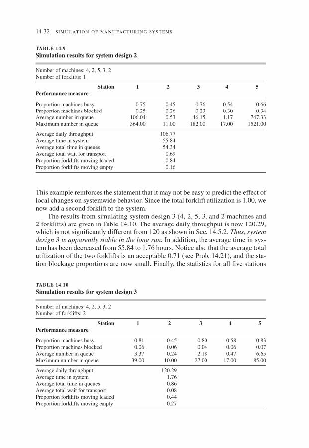
The results from simulating system design 2 (4, 2, 5, 3, and 2 machines for sta-tions 1, 2, . . . , 5 and 1 forklift) are given in Table 14.9. The average daily through-put has gone from 94.94 to 106.77, but is still considerably less than that expected for a well-defi ned system. Likewise the average time in system has been reduced from 109.20 to 55.84 hours. Even though we added three machines to the system, the queue statistics at station 5 have actually become considerably worse. (Why? See Prob. 14.20.) In fact, station 5 is now busy or blocked 100 percent of the time. Also, the blockage proportions have increased for four out of the fi ve stations.
FIGURE 14.27Number in queue 2 in time increments of 1 hour for system design 1 (replication 1).
250
00 40 80 120 160 200
Hours
50
100
150
200
Num
ber
in q
ueu
e 2
Law01323_ch14_001-047.indd Page 14-31 23/10/13 4:31 PM user-f-w-198 Law01323_ch14_001-047.indd Page 14-31 23/10/13 4:31 PM user-f-w-198 /203/MH02090/Law01323_disk1of1/0073401323/Law01323_pagefiles/203/MH02090/Law01323_disk1of1/0073401323/Law01323_pagefiles
14-32 simulation of manufacturing systems
TABLE 14.9
Simulation results for system design 2
Number of machines: 4, 2, 5, 3, 2Number of forklifts: 1
Station 1 2 3 4 5Performance measure
Proportion machines busy 0.75 0.45 0.76 0.54 0.66Proportion machines blocked 0.25 0.26 0.23 0.30 0.34Average number in queue 106.04 0.53 46.15 1.17 747.33Maximum number in queue 364.00 11.00 182.00 17.00 1521.00
Average daily throughput 106.77Average time in system 55.84Average total time in queues 54.34Average total wait for transport 0.69Proportion forklifts moving loaded 0.84Proportion forklifts moving empty 0.16
TABLE 14.10
Simulation results for system design 3
Number of machines: 4, 2, 5, 3, 2Number of forklifts: 2
Station 1 2 3 4 5Performance measure
Proportion machines busy 0.81 0.45 0.80 0.58 0.83Proportion machines blocked 0.06 0.06 0.04 0.06 0.07Average number in queue 3.37 0.24 2.18 0.47 6.65Maximum number in queue 39.00 10.00 27.00 17.00 85.00
Average daily throughput 120.29Average time in system 1.76Average total time in queues 0.86Average total wait for transport 0.08Proportion forklifts moving loaded 0.44Proportion forklifts moving empty 0.27
This example reinforces the statement that it may not be easy to predict the effect of local changes on systemwide behavior. Since the total forklift utilization is 1.00, we now add a second forklift to the system.
The results from simulating system design 3 (4, 2, 5, 3, and 2 machines and 2 forklifts) are given in Table 14.10. The average daily throughput is now 120.29, which is not signifi cantly different from 120 as shown in Sec. 14.5.2. Thus, system design 3 is apparently stable in the long run. In addition, the average time in sys-tem has been decreased from 55.84 to 1.76 hours. Notice also that the average total utilization of the two forklifts is an acceptable 0.71 (see Prob. 14.21), and the sta-tion blockage proportions are now small. Finally, the statistics for all fi ve stations
Law01323_ch14_001-047.indd Page 14-32 06/11/13 9:29 PM user-f-w-198 Law01323_ch14_001-047.indd Page 14-32 06/11/13 9:29 PM user-f-w-198 /203/MH02090/Law01323_disk1of1/0073401323/Law01323_pagefiles/203/MH02090/Law01323_disk1of1/0073401323/Law01323_pagefiles

chapter fourteen 14-33
FIGURE 14.28Number in queue 2 in time increments of 1 hour for system design 3 (replication 1).
4
3
2
1
00 40 80 120 160 200
Hours
Num
ber
in q
ueu
e 2
seem reasonable (see also Fig. 14.28), with the possible exception of the maximum queue sizes for stations 1 and 5. Whether queue sizes of 39 and 85 are acceptable depends on the particular application. These maximum queue sizes could be made smaller by adding additional machines to stations 1 and 5, respectively. Finally, note that average time in system (1.761) is equal to the sum of average total time in queues (0.861), average total wait for transport (0.075), average transport time (0.059), and average total service time (0.766)—the last two times are not shown in Table 14.10.
In going from system design 1 to system design 2, we added machines to sta-tions 2, 3, and 4 simultaneously. Therefore, it is reasonable to ask whether all three machines are actually necessary to achieve an expected throughput of 120. We fi rst removed one machine from station 2 for system design 3 (total number of machines is now 15) and obtained an average daily throughput of 119.38, which is signifi -cantly different from 120 (see Sec. 14.5.2 for the methodology used). Thus, two machines are required for station 2. Next, we removed one machine from station 3 for system design 3 (total number of machines is 15) and obtained an average daily throughput of 115.07, which is once again signifi cantly different from 120. Thus, we need fi ve machines for station 3. Finally, we removed one machine from station 4 for system design 3 and obtained system design 4, whose simulation results are given in Table 14.11. The throughput is unchanged, but the average time in system has increased from 1.76 to 2.61. This latter difference is statistically signifi cant as shown in Sec. 14.5.2. Note also that the average and maximum numbers in queue for station 4 are larger for system design 4, as expected.
Law01323_ch14_001-047.indd Page 14-33 23/10/13 4:31 PM user-f-w-198 Law01323_ch14_001-047.indd Page 14-33 23/10/13 4:31 PM user-f-w-198 /203/MH02090/Law01323_disk1of1/0073401323/Law01323_pagefiles/203/MH02090/Law01323_disk1of1/0073401323/Law01323_pagefiles

14-34 simulation of manufacturing systems
TABLE 14.11
Simulation results for system design 4
Number of machines: 4, 2, 5, 2, 2Number of forklifts: 2
Station 1 2 3 4 5Performance measure
Proportion machines busy 0.81 0.45 0.80 0.87 0.83Proportion machines blocked 0.06 0.06 0.04 0.08 0.07Average number in queue 2.89 0.25 1.88 14.31 6.50Maximum number in queue 32.00 11.00 27.00 90.00 81.00
Average daily throughput 120.29Average time in system 2.61Average total time in queues 1.72Average total wait for transport 0.07Proportion forklifts moving loaded 0.44Proportion forklifts moving empty 0.27
TABLE 14.12
Simulation results for system design 5
Number of machines: 4, 2, 5, 3, 2Number of forklifts: 2FIFO queue for forklifts
Station 1 2 3 4 5Performance measure
Proportion machines busy 0.81 0.45 0.80 0.58 0.83Proportion machines blocked 0.08 0.08 0.06 0.08 0.08Average number in queue 4.77 0.29 2.70 0.58 8.28Maximum number in queue 51.00 11.00 33.00 17.00 95.00
Average daily throughput 120.33Average time in system 2.03Average total time in queues 1.11Average total wait for transport 0.10Proportion forklifts moving loaded 0.44Proportion forklifts moving empty 0.31
System designs 3 and 4 both seem to be stable in the long run. The design that is preferable depends on factors such as the cost of an additional machine for sta-tion 4 (design 3), the cost of extra fl oor space (design 4), the cost associated with a larger average time in system (design 4), and the cost associated with a larger average work-in-process (design 4).
We now consider another variation of system design 3. It involves, for the fi rst time, a change in the control logic for the system. In particular, jobs waiting for the forklifts are processed in a FIFO manner, rather than shortest distance fi rst as before. The results for system design 5 are given in Table 14.12. Average time
Law01323_ch14_001-047.indd Page 14-34 23/10/13 4:31 PM user-f-w-198 Law01323_ch14_001-047.indd Page 14-34 23/10/13 4:31 PM user-f-w-198 /203/MH02090/Law01323_disk1of1/0073401323/Law01323_pagefiles/203/MH02090/Law01323_disk1of1/0073401323/Law01323_pagefiles

chapter fourteen 14-35
in system has gone from 1.76 to 2.03 hours, an apparent 15 percent increase. (Histograms of time in system for system designs 3 and 5, based on all 10 runs of each, are given in Fig. 14.29.) The queue statistics for station 1 have also increased by an appreciable amount, and the forklifts now spend more time moving empty. It takes a forklift more time to get to a waiting job, since the clos-est one is not generally chosen. We therefore do not recommend the new forklift-dispatching rule.
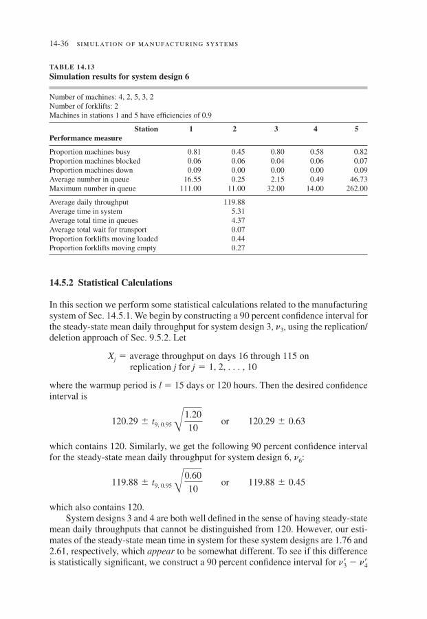
Finally, we discuss another variation of system design 3 (shortest-distance-fi rst forklift-dispatching rule), where certain machines break down. In particular, we assume that each machine in stations 1 and 5 breaks down independently with an effi ciency of 0.9 (see Sec. 14.4.2). The amount of busy time that a machine operates before failure is exponentially distributed with a mean of 4.5 hours, and repair times have a gamma distribution with a shape parameter of 2 and a mean of 0.5 hour. The simulation output for the resulting system design 6 is given in Table 14.13. The average daily throughput is now 119.88, but this is not signifi cantly different from 120 (see Sec. 14.5.2). On the other hand, average time in system has gone from 1.76 to 5.31, an increase of 202 percent. The queue statistics for stations 1 and 5 are also appreciably larger. Thus, breaking down only stations 1 and 5 caused a signifi cant degradation in system performance; breaking down all fi ve stations would probably have an even greater impact. In summary, we have once again seen the importance of modeling machine breakdowns correctly.
0.250.00
0.05
0.10
0.15
0.20
0.25
0.30
1.25 2.25 3.25 4.25 5.25 6.25 7.25
Shortest distance first (3)
FIFO (5)
h(x)
x
FIGURE 14.29Histograms of time in system for system designs 3 and 5.
Law01323_ch14_001-047.indd Page 14-35 23/10/13 4:31 PM user-f-w-198 Law01323_ch14_001-047.indd Page 14-35 23/10/13 4:31 PM user-f-w-198 /203/MH02090/Law01323_disk1of1/0073401323/Law01323_pagefiles/203/MH02090/Law01323_disk1of1/0073401323/Law01323_pagefiles
14-36 simulation of manufacturing systems
14.5.2 Statistical Calculations
In this section we perform some statistical calculations related to the manufacturing system of Sec. 14.5.1. We begin by constructing a 90 percent confi dence interval for the steady-state mean daily throughput for system design 3, n3, using the replication/deletion approach of Sec. 9.5.2. Let
Xj 5 average throughput on days 16 through 115 on replication j for j 5 1, 2, . . . , 10
where the warmup period is l 5 15 days or 120 hours. Then the desired confi dence interval is
120.29 6 t9, 0.95 B1.20
10 or 120.29 6 0.63
which contains 120. Similarly, we get the following 90 percent confi dence interval for the steady-state mean daily throughput for system design 6, n6:
119.88 6 t9, 0.95 B0.60
10 or 119.88 6 0.45
which also contains 120.System designs 3 and 4 are both well defi ned in the sense of having steady-state
mean daily throughputs that cannot be distinguished from 120. However, our esti-mates of the steady-state mean time in system for these system designs are 1.76 and 2.61, respectively, which appear to be somewhat different. To see if this difference is statistically signifi cant, we construct a 90 percent confi dence interval for n93 2 n94
TABLE 14.13
Simulation results for system design 6
Number of machines: 4, 2, 5, 3, 2Number of forklifts: 2Machines in stations 1 and 5 have effi ciencies of 0.9
Station 1 2 3 4 5Performance measure
Proportion machines busy 0.81 0.45 0.80 0.58 0.82Proportion machines blocked 0.06 0.06 0.04 0.06 0.07Proportion machines down 0.09 0.00 0.00 0.00 0.09Average number in queue 16.55 0.25 2.15 0.49 46.73Maximum number in queue 111.00 11.00 32.00 14.00 262.00
Average daily throughput 119.88Average time in system 5.31Average total time in queues 4.37Average total wait for transport 0.07Proportion forklifts moving loaded 0.44Proportion forklifts moving empty 0.27
Law01323_ch14_001-047.indd Page 14-36 23/10/13 4:31 PM user-f-w-198 Law01323_ch14_001-047.indd Page 14-36 23/10/13 4:31 PM user-f-w-198 /203/MH02090/Law01323_disk1of1/0073401323/Law01323_pagefiles/203/MH02090/Law01323_disk1of1/0073401323/Law01323_pagefiles
chapter fourteen 14-37
using the replication/deletion approach (see Example 10.5), where n9i is the steady-state mean time in system for system design i (where i 5 3, 4). We get
20.85 6 t9, 0.95 B0.22
10 or 20.85 6 0.27
which does not contain 0. Thus, n93 is signifi cantly different from n94.The results presented in Sec. 14.5.1 (and here) assume a warmup period of
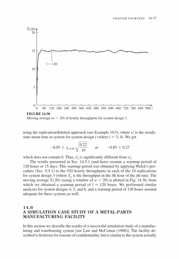
120 hours or 15 days. This warmup period was obtained by applying Welch’s pro-cedure (Sec. 9.5.1) to the 920 hourly throughputs in each of the 10 replications for system design 3 (where Yji is the throughput in the ith hour of the jth run). The moving average Yi(20) (using a window of w 5 20) is plotted in Fig. 14.30, from which we obtained a warmup period of l 5 120 hours. We performed similar analyses for system designs 4, 5, and 6, and a warmup period of 120 hours seemed adequate for these systems as well.
14.6 A SIMULATION CASE STUDY OF A METAL-PARTS MANUFACTURING FACILITY
In this section we describe the results of a successful simulation study of a manufac-turing and warehousing system [see Law and McComas (1988)]. The facility de-scribed is fi ctitious for reasons of confi dentiality, but is similar to the system actually
FIGURE 14.30Moving average (w 5 20) of hourly throughputs for system design 3.
20
00 90084078072066060054048042036030024018012060
5
10
15
Yi(20)
i
l � 120
Law01323_ch14_001-047.indd Page 14-37 23/10/13 4:31 PM user-f-w-198 Law01323_ch14_001-047.indd Page 14-37 23/10/13 4:31 PM user-f-w-198 /203/MH02090/Law01323_disk1of1/0073401323/Law01323_pagefiles/203/MH02090/Law01323_disk1of1/0073401323/Law01323_pagefiles

14-38 simulation of manufacturing systems
modeled for a Fortune 500 company. The project objectives, the simulation steps, and the benefi ts that we describe are also very similar to the actual ones.
14.6.1 Description of the System
The manufacturing facility (see Fig. 14.31) produces several different metal parts, each requiring three distinct subassemblies. Subassemblies corresponding to a particular part are produced in large batches on one of two subassembly manufac-turing lines, and then moved by conveyor to a loader where they are placed into empty containers. Each container holds only one type of subassembly at a time. The containers are stored in a warehouse until all three of the part subassemblies are available for assembly. Containers of the three subassemblies corresponding to a particular part are brought to an unloader/assembler (henceforth called the assembler), where they are unloaded and assembled into the fi nal product, which is then sent to shipping. The resulting empty containers are temporarily stored in a fi nite-capacity accumulating conveyor (not shown in the fi gure) at the back of the assembler. They are then taken to the loaders, if needed; otherwise, they are transported to the warehouse. Full and empty containers are moved by forklift trucks.
The assembler operates only 5 days a week, while the remainder of the system is in operation three shifts a day for 7 days a week. Also, the subassembly lines, the loaders, and the assembler are subject to random breakdowns.
14.6.2 Overall Objectives and Issues to Be Investigated
The subassembly lines already existed at the time of the study. However, the load-ers, the warehouse, and the assembler were in the process of being designed. (They
Warehouse
Empty
containers
Full
containers
Unloaders/assembler
Completed
products
to shipping
Full
Full
Empty
Empty
Loaders
Conveyors
from
subassembly
manufacturing
empty container
empty position
full container
FIGURE 14.31Layout of the system.
Law01323_ch14_001-047.indd Page 14-38 23/10/13 4:31 PM user-f-w-198 Law01323_ch14_001-047.indd Page 14-38 23/10/13 4:31 PM user-f-w-198 /203/MH02090/Law01323_disk1of1/0073401323/Law01323_pagefiles/203/MH02090/Law01323_disk1of1/0073401323/Law01323_pagefiles

chapter fourteen 14-39
were to replace existing technology that had certain throughput limitations.) As a result, the major objectives of the study were to see if the proposed system compo-nents would interact with each other effectively to produce the desired throughput, and also to determine the optimal system resource levels, such as the number of containers.
The specifi c issues investigated in the study included the following:
• Number of containers required• Number of forklift trucks required and their control logic• Number of “staged” containers desired in the input queues of the loaders and the
assembler (cannot be exceeded)• Number of output queue positions for the loaders• Number of required shifts for the assembler
Containers are staged in an input queue to keep the corresponding machine from becoming starved. In the case of a starved loader, the attached subassembly line is also stopped. If the output queue for a loader is full when a container com-pletes being loaded, then the loader is blocked and the corresponding subassembly line is also stopped.
14.6.3 Development of the Model
The study described here took 3 person-months to complete. An important part of the model-building process was the following series of meetings:
• Three-day initial meeting to defi ne project objectives, delineate model assump-tions, and specify data requirements
• One-day meeting (before programming) to perform a structured walk-through of the model assumptions (see Sec. 5.4.3) before an audience of the client’s engineers and managers
• One-day meeting to review initial simulation results and to make changes to model assumptions
As a result of the initial meeting, the company supplied us with a large amount of data that already existed in its computer databases and reports; however, a signifi -cant effort was required by both parties to get the data into a usable format. The UniFit statistical package (the predecessor of ExpertFit as described in Sec. 6.7) was used to analyze the data and to determine the appropriate probability distribu-tion for each source of system randomness. Highlights of our fi ndings are given in Table 14.14. In some cases standard distributions such as lognormal or Weibull were used; in other cases, an empirical distribution (see Sec. 6.2.4) based on the actual data was necessary.
The simulation model was programmed in the SIMAN (the predecessor of Arena as discussed in Sec. 3.5.1) simulation package, although other simulation packages could have been used as well. SIMAN was selected because of its fl exibility and material-handling features. The model consisted of approximately 2000 lines of code, 75 percent of which consisted of FORTRAN event routines. This model
Law01323_ch14_001-047.indd Page 14-39 23/10/13 4:31 PM user-f-w-198 Law01323_ch14_001-047.indd Page 14-39 23/10/13 4:31 PM user-f-w-198 /203/MH02090/Law01323_disk1of1/0073401323/Law01323_pagefiles/203/MH02090/Law01323_disk1of1/0073401323/Law01323_pagefiles

14-40 simulation of manufacturing systems
complexity was necessitated by a complicated set of rules (not described here) for each part that specify when its corresponding subassemblies are sent to the assembler.
14.6.4 Model Verifi cation and Validation
Verifi cation is concerned with determining if the simulation computer program is working as intended, and the initial verifi cation efforts included the following:
• The model was programmed and debugged in steps.• An interactive debugger was used to verify that each program path was correct.• Model output results were checked for reasonableness.• Model summary statistics for the values generated from the input probability
distributions were compared with historical-data summary statistics.
In addition, two more “defi nitive” verifi cation checks were performed. From the historical average busy times and average repair times, it was possible to com-pute the theoretical effi ciency (see Sec. 14.4.2) for each line. These effi ciencies and comparable ones produced by the simulation model (for scenario 1 in Table 14.17) are given in Table 14.15. The closeness of the effi ciencies indicates that the program for the subassembly lines was probably correct.
Using the simulation effi ciencies from Table 14.15 and three shifts for the assembler, it was possible to compute a theoretical effi ciency of 0.643 for the assembler. On the other hand, the simulation model actually produced an assembler effi ciency of 0.630. The closeness of these two effi ciencies indicates that the pro-gram for the assembler is probably correct.
TABLE 14.14
Probability distributions for the model
Source of randomness Distribution type
Subassembly line busy times EmpiricalSubassembly line repair times EmpiricalSubassembly line setup times TriangularLoader busy times EmpiricalLoader repair times LognormalAssembler busy times WeibullAssembler repair times LognormalAssembler setup times Uniform
TABLE 14.15
Verifi cation comparison of subassembly-line effi ciencies
Line Theoretical effi ciency Simulation effi ciency
1 0.732 0.741 2 0.724 0.727
Law01323_ch14_001-047.indd Page 14-40 23/10/13 4:31 PM user-f-w-198 Law01323_ch14_001-047.indd Page 14-40 23/10/13 4:31 PM user-f-w-198 /203/MH02090/Law01323_disk1of1/0073401323/Law01323_pagefiles/203/MH02090/Law01323_disk1of1/0073401323/Law01323_pagefiles

chapter fourteen 14-41
Validation is concerned with determining how closely the simulation model represents the actual system, and the following were some of the validation proce-dures performed:
• All model assumptions were reviewed and agreed upon by company personnel.• Different data sets for the same type of randomness (e.g., subassembly busy times
for the two lines) were tested for homogeneity and merged only if appropriate (see Sec. 6.13).
• All fi tted probability distributions (e.g., lognormal) were tested for correctness using the techniques of Chap. 6.
It is generally impossible to validate a simulation model completely, since some part of the actual system will not currently exist. However, building a simulation model of a similar existing system and comparing model and system outputs will often be the most defi nitive validation technique available. In our case, the sub-assembly lines were already in operation, while the rest of the system was in the design phase. In Table 14.16 is a comparison for each subassembly line of the his-torical effi ciency and the simulation effi ciency. The historical effi ciencies were taken from system output data available in a company report and were not used in building the model. (The theoretical effi ciencies in Table 14.15 were computed from historical system input data.) The agreement of the effi ciencies in Table 14.16 indicates that the model of the subassembly lines is “valid.”
14.6.5 Results of the Simulation Experiments
We fi rst simulated seven different scenarios (system designs), which are described in Table 14.17. Each of these scenarios assumed 3000 containers and used the fol-lowing company-specifi ed priority rule for dispatching forklift trucks:
1. Take empty containers to loaders.2. Pick up full containers from loaders.3. Take full containers to assembler.4. Pick up empty containers from assembler.
Five independent simulation runs were made for each scenario, with each run being 23 weeks in length and having a 3-week warmup period during which no statistics were gathered. The length of the warmup period was determined by plotting the average number of empty containers (over the fi ve runs) in time increments of 1 hour for scenario 1, which is shown in Fig. 14.32; initially, all containers were empty. Note that this empty-containers stochastic process does not have a steady-state
TABLE 14.16
Validation comparison of subassembly line effi ciencies
Line Historical effi ciency Simulation effi ciency
1 0.738 0.741 2 0.746 0.727
Law01323_ch14_001-047.indd Page 14-41 23/10/13 4:31 PM user-f-w-198 Law01323_ch14_001-047.indd Page 14-41 23/10/13 4:31 PM user-f-w-198 /203/MH02090/Law01323_disk1of1/0073401323/Law01323_pagefiles/203/MH02090/Law01323_disk1of1/0073401323/Law01323_pagefiles

14-42 simulation of manufacturing systems
distribution for scenarios 1 through 6 because the assembler does not operate on weekends. What about scenario 7 (see Prob. 14.25)?
A summary (average across the fi ve runs) of the seven sets of simulation runs appears in Table 14.18. Note that the throughput (in parts per week) for scenario 2 (two shifts) is considerably less than that for scenario 1 (three shifts). Also, scenario 2 has a high starvation proportion for the loaders. These results are due to a shortage of empty containers for scenario 2 caused by the assembler not operating enough. Observe for scenario 3 (two forklift trucks) that the throughput is again less than that for scenario 1 and, in addition, the blockage proportion is high for the assem-bler. This is due to the unavailability of forklift trucks to remove empty containers from the assembler’s conveyor caused by the nonoptimal priority rule (i.e., pick up at the assembler has the lowest priority); see Table 14.20. Note that queue sizes of one (scenario 4) cause a small degradation in throughput. Finally, the high forklift-truck
TABLE 14.17
Scenarios for the initial simulation runs
Scenario Forklift trucks Queue sizes Assembler shifts
1 3 2 3 2 3 2 2 3 2 2 3 4 3 1 3 5 3 3 3 6 3, 2 (weekend) 2 3 7 3 2 2 (all 7 days)
3000
1229
01 504 3864
Hours
Num
ber
of
empty
conta
iner
s
FIGURE 14.32Average number of empty containers (over the fi ve runs) in time increments of 1 hour for scenario 1.
Law01323_ch14_001-047.indd Page 14-42 23/10/13 4:31 PM user-f-w-198 Law01323_ch14_001-047.indd Page 14-42 23/10/13 4:31 PM user-f-w-198 /203/MH02090/Law01323_disk1of1/0073401323/Law01323_pagefiles/203/MH02090/Law01323_disk1of1/0073401323/Law01323_pagefiles

chapter fourteen 14-43
idle proportions in Table 14.18 are caused by the periods of inactivity for the loaders and the assembler.
The system description and simulation results described above were presented to approximately 20 of the company’s employees including the plant manager. As a result of this meeting, it was decided to simulate the six additional scenarios de-scribed in Table 14.19. Each of these scenarios had queue sizes of 2, three assembler shifts, and the same run length and number of runs as before.
A summary of the simulation results for these scenarios (and also scenario 1 from Table 14.18) is given in Table 14.20. Note that the throughput does not change signifi cantly when the number of containers is varied between 2250 and 3000. This can be seen more clearly in Fig. 14.33, where throughput is plotted as a function of the number of containers. Observe also that the shortest-distance-fi rst dispatching rule (scenario 13) gives somewhat better results for two forklift trucks than the original rule (compare scenarios 13 and 3).
14.6.6 Conclusions and Benefi ts
Based on the simulation results presented above and several conversations with the client, the following project conclusions were reached:
• The company will probably buy 2250 containers rather than the 3000 containers originally budgeted.
• Three assembler shifts (Monday through Friday) are required.
TABLE 14.18
Summary of simulation results for initial set of runs
Avg. empty Parts Loader Assembler ForkliftScenario containers per week starved blocked idle
1 1229 15,019 0.000 0.001 0.370 2 241 11,405 0.157 0.001 0.489 3 442 13,109 0.050 0.133 0.210 4 1218 14,666 0.001 0.001 0.381 5 1233 15,050 0.000 0.001 0.386 6 1234 15,050 0.000 0.001 0.317 7 1123 15,079 0.000 0.001 0.369
TABLE 14.19
Scenarios for the second set of simulation runs
Scenario Number of containers Forklift trucks
8 2750 3 9 2500 3 10 2250 3 11 2000 3 12 1750 3 13 3000 2*
* Dispatching rule is shortest distance fi rst.
Law01323_ch14_001-047.indd Page 14-43 23/10/13 4:31 PM user-f-w-198 Law01323_ch14_001-047.indd Page 14-43 23/10/13 4:31 PM user-f-w-198 /203/MH02090/Law01323_disk1of1/0073401323/Law01323_pagefiles/203/MH02090/Law01323_disk1of1/0073401323/Law01323_pagefiles

14-44 simulation of manufacturing systems
• Two or three forklift trucks are required for Monday through Friday (further in-vestigation is needed), and two are required for Saturday and Sunday.
• Two containers should be staged in the input queues of the loaders and the assembler.
• The output queues of the loaders should have a capacity of two.• The system can achieve the desired throughput with the above specifi cations.
The company received several defi nite benefi ts as a result of the simulation study. First, they gained the assurance (before building the system) that the pro-posed design for the loaders, warehouse, and assembler would actually meet their
TABLE 14.20
Summary of simulation results for second set of runs
Avg. empty Parts Loader Assembler ForkliftScenario containers per week starved blocked idle
1 1229 15,019 0.000 0.001 0.370 8 941 14,959 0.006 0.001 0.379 9 640 14,798 0.014 0.001 0.384 10 402 14,106 0.053 0.001 0.411 11 209 11,894 0.192 0.000 0.487 12 80 8758 0.374 0.000 0.597 13 1410 14,306 0.005 0.002 0.265
10,000
1750 2000 2250 2500 2750 3000
15,000
Par
ts p
er w
eek
Number of containers
Likely company choice
FIGURE 14.33Throughput (parts per week) as a function of the number of containers.
Law01323_ch14_001-047.indd Page 14-44 23/10/13 4:31 PM user-f-w-198 Law01323_ch14_001-047.indd Page 14-44 23/10/13 4:31 PM user-f-w-198 /203/MH02090/Law01323_disk1of1/0073401323/Law01323_pagefiles/203/MH02090/Law01323_disk1of1/0073401323/Law01323_pagefiles

chapter fourteen 14-45
specifi ed throughput requirements. If a simulation study had not been performed and if a bottleneck were discovered after system installation, the cost of retrofi tting the system could have been signifi cant.
The company will probably buy 2250 containers rather than the 3000 originally in the budget, since the throughputs for scenarios 1, 8, 9, and 10 are all suffi cient for the projected product demand. Since containers cost $400 each, this is a savings of $300,000. In addition, each container occupies 20.3 square feet of fl oor space, and the company expects to rent fl oor space at a cost of $15 per square foot per year. Thus, by using 750 fewer containers, they will save $228,375 a year in fl oor-space rental. Therefore, the total fi rst-year savings are $528,375.
PROBLEMS
14.1. For the system with no breakdowns in Example 14.3, show that the machine tool has suffi cient processing capacity.
14.2. Consider a machine with uptimes U1, U2, . . . and downtimes D1, D2, . . . as described in Sec. 14.4.2. Is it completely correct to assume that the Ui’s and the Di’s are each IID within themselves? Why or why not?
14.3. For the machine in Prob. 14.2, is it completely correct to assume that Ui and Di are independent? Why or why not?
14.4. Consider a machine that operates continuously until a part jams; i.e., it is never starved or blocked. Suppose that a part has a probability p of jamming, independently of all other parts. What is the probability distribution of the number of parts produced before the fi rst jam and what is its mean? Thus, if the average number of parts pro-duced before a jam is known for an actual machine, the above model can be used to specify p for a simulation model.
14.5. Consider the calendar-time approach for modeling the up segments of a machine in Sec. 14.4.2. Suppose that a machine breaks down when it is starved. (Perhaps it was idling at the time.) Do you think that the breakdown would be discovered immediately (and repair begun) or when the next part actually arrives? Assume that availability of a repairman is not an issue.
14.6. Consider a machine that “operates” 24 hours a day for 7 days a week. The uptimes U1, U2, . . . and downtimes D1, D2, . . . are available, but not the corresponding busy times B1, B2, . . . . Suppose, for simplicity, that an exponential distribution fi ts the Ui’s. The average number of parts produced per 8-hour shift is known, as well as the aver-age processing time for parts. Assuming that the exponential distribution is also a good model for the Bi’s, what mean should be used for a machine-breakdown model based on busy time?
14.7. Consider a machine that is never starved or blocked. Suppose shop-fl oor personnel estimate that the machine has an effi ciency e 5 0.9 and typically fails twice in an 8-hour shift. What values of E(U) and E(D) should be used in modeling this machine?
Law01323_ch14_001-047.indd Page 14-45 23/10/13 4:31 PM user-f-w-198 Law01323_ch14_001-047.indd Page 14-45 23/10/13 4:31 PM user-f-w-198 /203/MH02090/Law01323_disk1of1/0073401323/Law01323_pagefiles/203/MH02090/Law01323_disk1of1/0073401323/Law01323_pagefiles

14-46 simulation of manufacturing systems
14.8. Suppose that a machine will fail when either of two independent components fails. Describe how you would model breakdowns for the machine for each of the follow-ing two cases:(a) The uptime of each machine is based on busy time.(b) The uptime of each machine is based on calendar time.
14.9. Consider a machine that is never starved or blocked. It will fail when either compo-nent A or component B fails. These components fail independently of each other, and one component does not “age” while the other component is down. The mean busy time before failure and the mean repair (down) time for these components (in hours) are as follows:
Component Mean busy time Mean repair time
A 46.5 1.5 B 250.0 6.0
Compute the effi ciency e of the machine.
14.10. Use a different method to compute the effi ciency in Prob. 14.9 if busy time before failure and repair time are both exponentially distributed.
14.11. Consider a machine that has two types of failure. Type 1 is a minor problem, which is corrected by the machine operator with a “short” repair (down) time. A type 2 failure, on the other hand, is a major problem requiring a maintenance person and a “long” repair time. Suppose that n observations on repair times are available for the machine and ni of them are of type i (where i 5 1, 2), with n1 1 n2 5 n. Give two possible approaches for representing repair times in a simulation model. What are you implicitly assuming about the relationship between Ui and Di (equal to Ri here)?
14.12. Simulate system design 3 in Sec. 14.5 with the change that an idle forklift has station 6 (input/output) as its home base. That is, an idle forklift will travel to station 6 to wait for its next job. Which of the two system designs is preferable?
14.13. For the manufacturing system in Sec. 14.5, why is the mean total service time aver-aged over all jobs equal to 0.77?
14.14. Using simulation, determine the required number of machines for each workstation and the required number of forklifts for the manufacturing system in Sec. 14.5 (original version) if each workstation has an infi nite-capacity output queue. Thus, no blocking occurs.
14.15. For the manufacturing system in Sec. 14.5, why can the expected throughput not exceed 120 jobs per 8-hour day?
14.16. What is missing in Sec. 14.5 from the analytic calculations to determine the number of machines for each station? Hint: Can a machine always process a waiting part?
14.17. What is missing in Sec. 14.5 from the analytic calculations to determine the number of forklifts?
Law01323_ch14_001-047.indd Page 14-46 23/10/13 4:31 PM user-f-w-198 Law01323_ch14_001-047.indd Page 14-46 23/10/13 4:31 PM user-f-w-198 /203/MH02090/Law01323_disk1of1/0073401323/Law01323_pagefiles/203/MH02090/Law01323_disk1of1/0073401323/Law01323_pagefiles
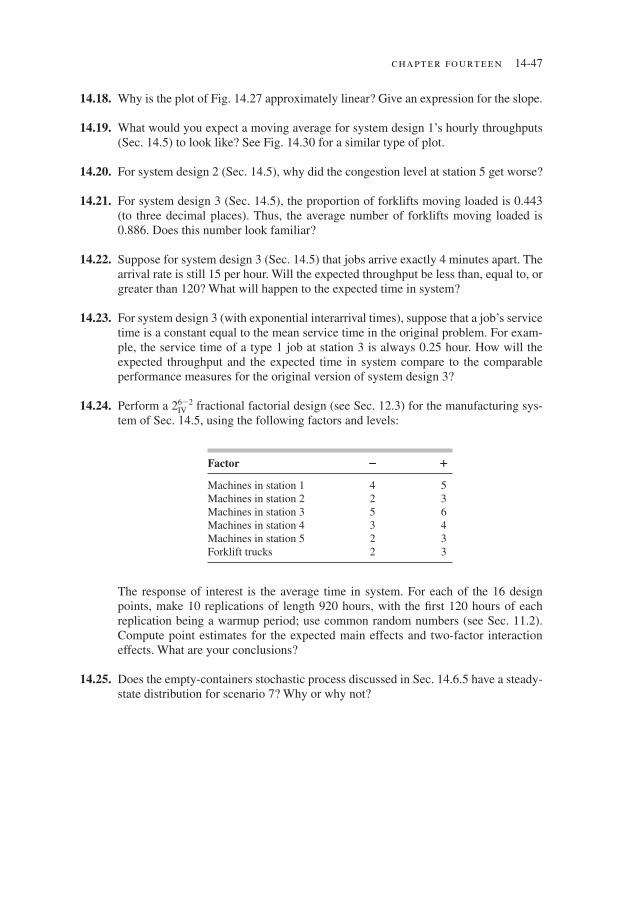
chapter fourteen 14-47
14.18. Why is the plot of Fig. 14.27 approximately linear? Give an expression for the slope.
14.19. What would you expect a moving average for system design 1’s hourly throughputs (Sec. 14.5) to look like? See Fig. 14.30 for a similar type of plot.
14.20. For system design 2 (Sec. 14.5), why did the congestion level at station 5 get worse?
14.21. For system design 3 (Sec. 14.5), the proportion of forklifts moving loaded is 0.443 (to three decimal places). Thus, the average number of forklifts moving loaded is 0.886. Does this number look familiar?
14.22. Suppose for system design 3 (Sec. 14.5) that jobs arrive exactly 4 minutes apart. The arrival rate is still 15 per hour. Will the expected throughput be less than, equal to, or greater than 120? What will happen to the expected time in system?
14.23. For system design 3 (with exponential interarrival times), suppose that a job’s service time is a constant equal to the mean service time in the original problem. For exam-ple, the service time of a type 1 job at station 3 is always 0.25 hour. How will the expected throughput and the expected time in system compare to the comparable performance measures for the original version of system design 3?
14.24. Perform a 2622IV fractional factorial design (see Sec. 12.3) for the manufacturing sys-
tem of Sec. 14.5, using the following factors and levels:
The response of interest is the average time in system. For each of the 16 design points, make 10 replications of length 920 hours, with the fi rst 120 hours of each replication being a warmup period; use common random numbers (see Sec. 11.2). Compute point estimates for the expected main effects and two-factor interaction effects. What are your conclusions?
14.25. Does the empty-containers stochastic process discussed in Sec. 14.6.5 have a steady-state distribution for scenario 7? Why or why not?
Factor 2 1
Machines in station 1 4 5Machines in station 2 2 3Machines in station 3 5 6Machines in station 4 3 4Machines in station 5 2 3Forklift trucks 2 3
Law01323_ch14_001-047.indd Page 14-47 23/10/13 4:31 PM user-f-w-198 Law01323_ch14_001-047.indd Page 14-47 23/10/13 4:31 PM user-f-w-198 /203/MH02090/Law01323_disk1of1/0073401323/Law01323_pagefiles/203/MH02090/Law01323_disk1of1/0073401323/Law01323_pagefiles