simulation of human ischemic stroke in realistic 3d geometry · simulation of human ischemic stroke...
TRANSCRIPT
HAL Id: hal-00546223https://hal.archives-ouvertes.fr/hal-00546223v3
Submitted on 16 May 2012
HAL is a multi-disciplinary open accessarchive for the deposit and dissemination of sci-entific research documents, whether they are pub-lished or not. The documents may come fromteaching and research institutions in France orabroad, or from public or private research centers.
L’archive ouverte pluridisciplinaire HAL, estdestinée au dépôt et à la diffusion de documentsscientifiques de niveau recherche, publiés ou non,émanant des établissements d’enseignement et derecherche français ou étrangers, des laboratoirespublics ou privés.
Simulation of human ischemic stroke in realistic 3Dgeometry
Thierry Dumont, Max Duarte, Stéphane Descombes, Marie-Aimée Dronne,Marc Massot, Violaine Louvet
To cite this version:Thierry Dumont, Max Duarte, Stéphane Descombes, Marie-Aimée Dronne, Marc Massot, et al.. Sim-ulation of human ischemic stroke in realistic 3D geometry. Communications in Nonlinear Science andNumerical Simulation, Elsevier, 2013, 18 (6), pp.1539-1557. <10.1016/j.cnsns.2012.10.002>. <hal-00546223v3>
Simulation of human ischemic stroke in realistic 3D geometry
Thierry Dumonta,b,∗, Max Duartec,d, Stephane Descombesd,e, Marie-Aimee Dronnef,b, MarcMassotc, Violaine Louveta
a Institut Camille Jordan - UMR CNRS 5208, Universite de Lyon, Universite Lyon 1, INSA de Lyon 69621, EcoleCentrale de Lyon, 43 Boulevard du 11 novembre 1918, 69622 Villeurbanne Cedex, France.
b INRIA, Project-team NUMED, Ecole Normale superieure de Lyon, 46 allee d’Italie, 69007 Lyon Cedex 07, France.cLaboratoire EM2C - UPR CNRS 288, Ecole Centrale Paris, Grande Voie des Vignes, 92295 Chatenay-Malabry Cedex,
France.dLaboratoire J. A. Dieudonne - UMR CNRS 6621, Universite de Nice - Sophia Antipolis, Parc Valrose, 06108 Nice
Cedex 02, France.eINRIA Sophia Antipolis - Mediterranee research center, Project-team NACHOS, 2004 Route des Lucioles, BP 93,
06902 Sophia Antipolis Cedex, France.fUniversite de Lyon, Universite Lyon 1, ISPB - Faculte de Pharmacie de Lyon 69003 Lyon, France.
Abstract
In silico research in medicine is thought to reduce the need for expensive clinical trials underthe condition of reliable mathematical models and accurate and efficient numerical methods. Inthe present work, we tackle the numerical simulation of reaction-diffusion equations modelinghuman ischemic stroke. This problem induces peculiar difficulties like potentially large stiffnesswhich stems from the broad spectrum of temporal scales in the nonlinear chemical source termas well as from the presence of steep spatial gradients in the reaction fronts, spatially very lo-calized. Furthermore, simulations on realistic 3D geometries are mandatory in order to describecorrectly this type of phenomenon. The main goal of this article is to obtain, for the first time,3D simulations on realistic geometries and to show that the simulation results are consistent withthose obtain in experimental studies or observed on MRI images in stroke patients.
For this purpose, we introduce a new resolution strategy based mainly on time operator split-ting that takes into account complex geometry coupled with a well-conceived parallelizationstrategy for shared memory architectures. We consider then a high order implicit time integra-tion for the reaction and an explicit one for the diffusion term in order to build a time operatorsplitting scheme that exploits efficiently the special features of each problem. Thus, we aim atsolving complete and realistic models including all time and space scales with conventional com-puting resources, that is on a reasonably powerful workstation. Consequently and as expected,2D and also fully 3D numerical simulations of ischemic strokes for a realistic brain geometry,are conducted for the first time and shown to reproduce the dynamics observed on MRI imagesin stroke patients. Beyond this major step, in order to improve accuracy and computational ef-ficiency of the simulations, we indicate how the present numerical strategy can be coupled withspatial adaptive multiresolution schemes. Preliminary results in the framework of simple geome-tries allow to assess the proposed strategy for further developments.
Keywords: Ischemic stroke, reaction-diffusion equations, operator splitting, parallel computing2010 MSC: 35A35, 35K57, 65L06, 65M08, 65M50, 65Y05, 92B05
Preprint submitted to scientific journal May 16, 2012
1. Introduction
Stroke is a major public health problem since it represents the second leading cause of deathworldwide and the first cause of acquired disability in adults. In the United States, this diseasestrikes once every 40 seconds and causes death every 4 minutes, with an estimated 41.6% deathrate in 2007 [1]. Most frequently (80%) strokes result from the occlusion of one or several brainvessels and are thus called ischemic strokes (in the other cases, strokes are hemorrhagic strokes).Ischemic stroke involves many pathophysiological mechanisms causing devastating neurologicaldamage (see for review [2, 3]). Understanding these mechanisms is of the most importance todevelop new therapeutic strategies since no treatments are currently available for most strokepatients. Currently, the only FDA-approved treatment for stroke patients is a thrombolytic agent(tPA) which can only be given to less than 10% of patients because of its narrow time-window andits hemorrhagic risks [4]. Many neuroprotective agents (aimed at blocking the ischemic cascade)have also been developed but, although they had given very promising results in preclinicalstudies in rodent models, they appeared ineffective or even noxious during the clinical trials instroke patients (see for review [5, 6, 7, 8]). This discrepancy between the results in rodents andin humans is partly due to the anatomic and histological differences between rodent and humanbrains. In this case, results in rodents are thus difficult to extrapolate to stroke patients. As aconsequence, a mathematical model and its numerical simulations can help both to test somebiological hypotheses concerning the involved mechanisms and to give new insights concerningthe effects of these neuroprotective agents.
Previous works have been conducted on stroke modeling. One of these models [9] is focusedon the main mechanisms leading to cell death during the first hour of an ischemic stroke (suchas ionic movements, glutamate excitotoxicity and cytotoxic edema). This model is based on asystem of ordinary differential equations (ODEs) and is mainly an electrophysiological model.It describes the dynamics of membrane potentials, cell volumes and ionic concentrations (K+,Na+, Cl−, Ca2+ and Glu−) in brain cells and in the extracellular space during a stroke. This modelwas used to study the role of various cell types during ischemia [10] and to explore the effectsof various neuroprotective agents in stroke patients [11]. Other models have been developed tosimulate and study spreading depressions during a stroke. This phenomenon is characterized bya slowly propagating depolarization of brain cells along with drastic disruption of ionic gradients[12]. These spreading depressions have recently been observed in stroke patients [13] and aresupposed to extent the ischemic damage [14]. Some models reproduce and study the behaviorof spreading depressions in neuronal cells [15, 16]. Others describe these depolarization wavesthough neuronal and glial cells [17]. Other models study the influence of the human brain cortexgeometry on the propagation of these spreading depressions [17, 18]. All these models are basedon reaction-diffusion systems and in this paper we choose to use the mathematical model [9].
The final goal of our work is to utterly describe and reproduce precocious mechanismsof stroke (i.e. ionic movements, glutamate excitotoxicity and cytotoxic edema) including thespreading depressions, for a realistic brain geometry. A first description of the algorithms usedfor the numerical solution of this stroke model on 1D and 2D geometries was presented in aprevious article [19]. However, since we need to take into account the anatomic and histological
∗Corresponding authorEmail addresses: [email protected] (Thierry Dumont), [email protected] (Max Duarte),
[email protected] (Stephane Descombes), [email protected](Marie-Aimee Dronne), [email protected] (Marc Massot), [email protected] (Violaine Louvet)
2

specificities of human brain, this model must be simulated on a 3D realistic geometry, whichimplies to develop powerful numerical methods able to deal with a broad spectrum of spatialand temporal scales. This paper focuses on the methods developed for the numerical solution ofthis model, with much more insights on the mathematical and numerical methods than in [19].The numerical method is based on operator splitting and explicit/implicit Runge-Kutta methods.A very important feature of this method is that no linear system (of large size) is solved. Wethen show, for the first time, numerical simulations in 3D obtained thanks to a particular im-plementation of parallelism in the framework of shared memory machines. Moreover, these 3Dsimulations are computed on realistic geometries, obtained from MRI of the human brain, onconventional computational resources, that is on nowadays reasonably powerful workstations;and they are shown to match the observed dynamics from MRI images in stroke patient. Sinceaccuracy in 3D simulations is not yet optimal, the ability of extending the proposed numericalstrategy to adaptive multiresolution is presented in the framework of preliminary computationsin simple geometries, based on a strategy introduced in [20]. The idea is to increase the level ofaccuracy in order to match all the spatial scales, with a better computational efficiency; thanksto the fact that phenomenons in strokes are spatially localized, a local mesh adaptation (likemultiresolution techniques) is the most suitable.
The paper is organized as follows: in a first part, we present the reaction-diffusion model ofthe precocious mechanisms. We then focus on numerical methods: we first mention the differentapproaches which can be used to discretize the system in time and explain why in the context ofsuch a stiff and large system only very few are relevant. We then present our numerical strategybased on splitting methods; a grid adaptation technique is also proposed as a possible improve-ment of the numerical strategy, considering particular features of the phenomena. We presentthe parallel implementation on shared memory machines of the numerical strategy, and discussthe numerical validation of the results. In the next section, 2D and 3D numerical results of sim-ulations with complex geometry are presented. Biological results obtained are compared withreal observations and discussed in the penultimate section. Biomarkers are used in order to vali-date these computations. A brief and prospective study based on coupling the proposed strategywith adaptive multiresolution in space is conducted, whereas conclusion and future works arepresented in the last section.
2. Stroke modeling through stiff Reaction–Diffusion systems
In this section, we describe the model on which our study is based. This model includes ionicmovements, glutamate excitotoxicity, cytotoxic edema and spreading depressions [9, 10]. It thusfocuses on the first hour of a stroke, when the ionic exchanges are the main mechanisms leadingto cell death. This model is based on a reaction-diffusion system (equations are given in whatfollows in Table 1).
In this model, brain tissue is composed of two cell types, namely neurons and glial cells,and of extracellular space. Two domains are considered: the white and the gray matter whichdiffer in their glial cell composition (astrocytes in gray matter and oligodendrocytes in whitematter) and in their “neuronal area” composition (neuronal somas in gray matter and neuronalaxons in white matter). Human brain cortex is exclusively composed of gray matter whereashuman brain space is mainly composed of white matter (except the gray kernels). For simplicityreasons, we consider in the model that brain cortex contains only gray matter and brain spacecontains only white matter. The ionic species considered in this model are K+, Na+, Cl−, Ca2+
and the Glutamate (glu). They pass through neuronal and glial membranes via ionic channels3
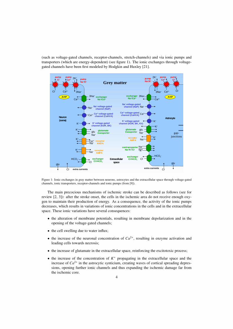
(such as voltage-gated channels, receptor-channels, stretch-channels) and via ionic pumps andtransporters (which are energy-dependent) (see figure 1). The ionic exchanges through voltage-gated channels have been first modeled by Hodgkin and Huxley [21].
Neuron(soma)
Astrocyte
Extracellularspace
3Na+
2K+
Ca2+Cl-
pump Ca2+
pump Cl-
Cl-Ca2+
pump Ca2+
pump Cl-
Ca2+ Ca2+ voltage-gated channel (CaHVA)
Na+ Na+ voltage-gated channel (NaP)
K+ K+ voltage-gated channel (KDR, BK)
Ca2+Ca2+ voltage-gated channel (CaHVA)
Na+Na+ voltage-gated
channel (NaP)
K+
3Na+
Ca2+
exchanger Na+/Ca2+
Ca2+
3Na+exchanger
Na+/Ca2+
K+
gluNa+glu
Na+
K+glutamate transporter
Na+
2Cl-K+
contransporterNa+/K+/Cl-
Cl-HCO3
-exchanger
Cl-/HCO3-
Cl-exchanger Cl-/HCO3
-HCO3
-
K+
Na+receptor
AMPAK+
Ca2+
Na+
K+
Na+
receptor NMDA
receptor AMPA
K+ voltage-gated channel (KDR, BK, Kir)
glutamate transporter
pump Na+/K+
3Na+
2K+pump Na+/K+
glu glu
Cl- Cl-extra currents extra currents
ATP ATP
Grey matter
gap-junctions
Figure 1: Ionic exchanges in gray matter between neurons, astrocytes and the extracellular space through voltage-gatedchannels, ionic transporters, receptor-channels and ionic pumps (from [9]).
The main precocious mechanisms of ischemic stroke can be described as follows (see forreview [2, 3]): after the stroke onset, the cells in the ischemic area do not receive enough oxy-gen to maintain their production of energy. As a consequence, the activity of the ionic pumpsdecreases, which results in variations of ionic concentrations in the cells and in the extracellularspace. These ionic variations have several consequences:
• the alteration of membrane potentials, resulting in membrane depolarization and in theopening of the voltage-gated channels;
• the cell swelling due to water influx;
• the increase of the neuronal concentration of Ca2+, resulting in enzyme activation andleading cells towards necrosis;
• the increase of glutamate in the extracellular space, reinforcing the excitotoxic process;
• the increase of the concentration of K+ propagating in the extracellular space and theincrease of Ca2+ in the astrocytic synticium, creating waves of cortical spreading depres-sions, opening further ionic channels and thus expanding the ischemic damage far fromthe ischemic core.
4
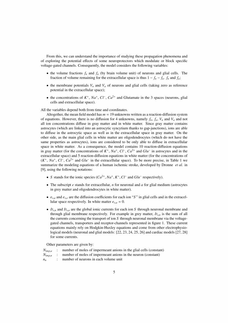
From this, we can understand the importance of studying these propagation phenomena andof exploring the potential effects of some neuroprotectors which modulate or block specificvoltage-gated channels. Consequently, the model considers the following variables:
• the volume fractions fn and fa (by brain volume unit) of neurons and glial cells. Thefraction of volume remaining for the extracellular space is thus 1 − fn − fa. fn and fa;
• the membrane potentials Vn and Va of neurons and glial cells (taking zero as referencepotential in the extracellular space);
• the concentrations of K+, Na+, Cl−, Ca2+ and Glutamate in the 3 spaces (neurons, glialcells and extracellular space).
All the variables depend both from time and coordinates.Altogether, the mean field model has m = 19 unknowns written as a reaction-diffusion system
of equations. However, there is no diffusion for 4 unknowns, namely fn, fa, Vn and Va and notall ion concentrations diffuse in gray matter and in white matter. Since gray matter containsastrocytes (which are linked into an astrocytic syncytium thanks to gap-junctions), ions are ableto diffuse in the astrocytic space as well as in the extracellular space in gray matter. On theother side, as the main glial cells in white matter are oligodendrocytes (which do not have thesame properties as astrocytes), ions are considered to be only able to diffuse in extracellularspace in white matter. As a consequence, the model contains 10 reaction-diffusion equationsin gray matter (for the concentrations of K+, Na+, Cl−, Ca2+ and Glu− in astrocytes and in theextracellular space) and 5 reaction-diffusion equations in white matter (for the concentrations of(K+, Na+, Cl−, Ca2+ and Glu− in the extracellular space). To be more precise, in Table 1 wesummarize the modeling equations of a human ischemic stroke, developed by Dronne et al. in[9], using the following notations:
• S stands for the ionic species (Ca2+,Na+,K+,Cl− and Glu− respectively).
• The subscript e stands for extracellular, n for neuronal and a for glial medium (astrocytesin grey matter and oligodendrocytes in white matter).
• εs,a and εs,e are the diffusion coefficients for each ion “S ” in glial cells and in the extracel-lular space respectively. In white matter εs,a = 0.
• Its,n and Its,a are the global ionic currents for each ion S through neuronal membrane andthrough glial membrane respectively. For example in grey matter, Its,n is the sum of allthe currents concerning the transport of ion S through neuronal membrane via the voltage-gated channels, transporters and receptor-channels represented in figure 1. These currentequations mainly rely on Hodgkin-Huxley equations and come from other electrophysio-logical models (neuronal and glial models: [22, 23, 24, 25, 26] and cardiac models [27, 28]for some currents.
Other parameters are given by:Nimp,a : number of moles of impermeant anions in the glial cells (constant)Nimp,n : number of moles of impermeant anions in the neuron (constant)nn : number of neurons in each volume unit
5
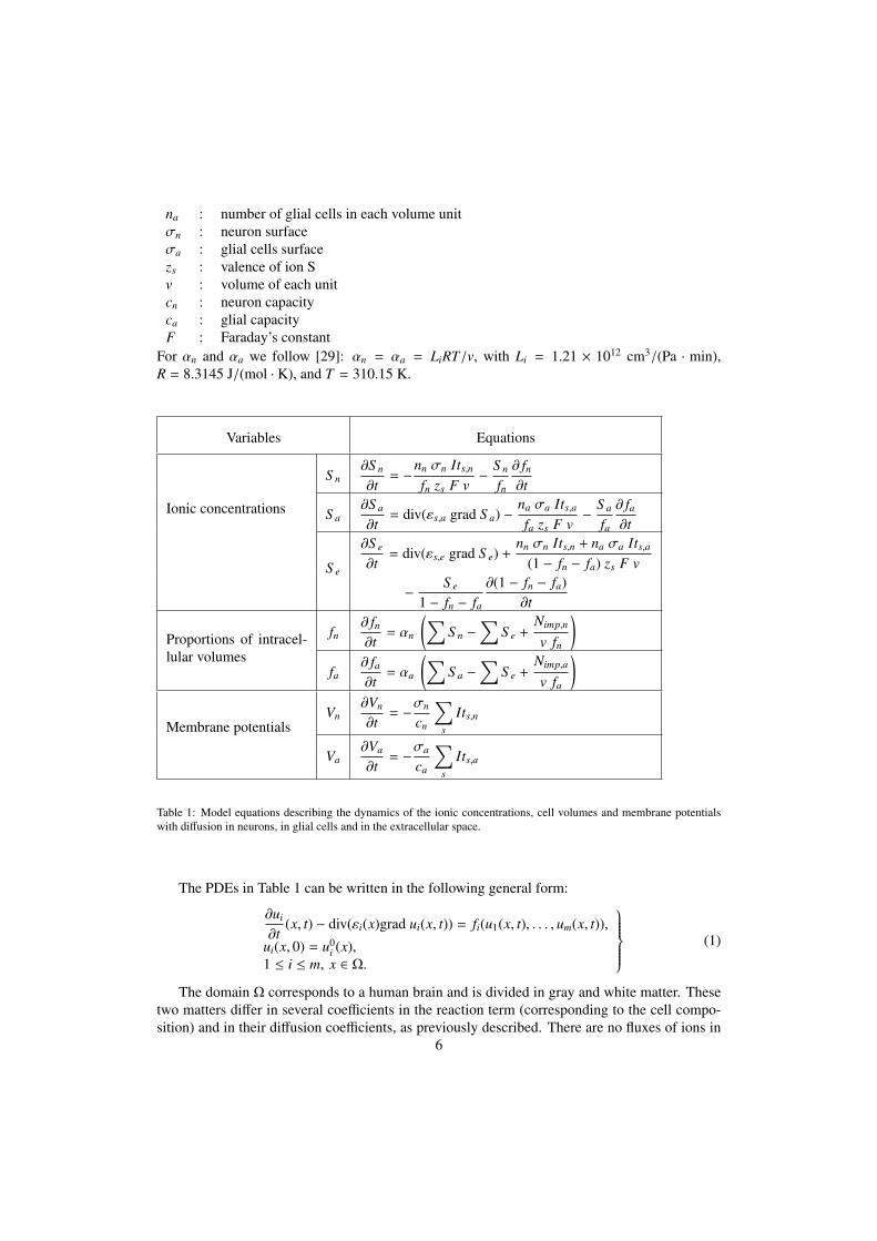
na : number of glial cells in each volume unitσn : neuron surfaceσa : glial cells surfacezs : valence of ion Sv : volume of each unitcn : neuron capacityca : glial capacityF : Faraday’s constant
For αn and αa we follow [29]: αn = αa = LiRT/v, with Li = 1.21 × 1012 cm3/(Pa · min),R = 8.3145 J/(mol · K), and T = 310.15 K.
Variables Equations
Ionic concentrations
S n∂S n
∂t= −
nn σn Its,n
fn zs F v−
S n
fn
∂ fn∂t
S a∂S a
∂t= div(εs,a grad S a) −
na σa Its,a
fa zs F v−
S a
fa
∂ fa∂t
S e
∂S e
∂t= div(εs,e grad S e) +
nn σn Its,n + na σa Its,a
(1 − fn − fa) zs F v
−S e
1 − fn − fa
∂(1 − fn − fa)∂t
Proportions of intracel-lular volumes
fn∂ fn∂t
= αn
(∑S n −
∑S e +
Nimp,n
v fn
)fa
∂ fa∂t
= αa
(∑S a −
∑S e +
Nimp,a
v fa
)
Membrane potentialsVn
∂Vn
∂t= −
σn
cn
∑s
Its,n
Va∂Va
∂t= −
σa
ca
∑s
Its,a
Table 1: Model equations describing the dynamics of the ionic concentrations, cell volumes and membrane potentialswith diffusion in neurons, in glial cells and in the extracellular space.
The PDEs in Table 1 can be written in the following general form:
∂ui
∂t(x, t) − div(εi(x)grad ui(x, t)) = fi(u1(x, t), . . . , um(x, t)),
ui(x, 0) = u0i (x),
1 ≤ i ≤ m, x ∈ Ω.
(1)
The domain Ω corresponds to a human brain and is divided in gray and white matter. Thesetwo matters differ in several coefficients in the reaction term (corresponding to the cell compo-sition) and in their diffusion coefficients, as previously described. There are no fluxes of ions in
6
and out of the brain and thus, the boundary conditions are of Neumann homogeneous type. Forthe initial conditions ui(x, 0) = u0
i (x), 1 ≤ i ≤ m, a classical medical hypothesis is that the systemis in a stable equilibrium: thus we take, and must find, a stable constant solution of system (1).
Let us mention some characteristics of the system which are very important in the choice ofnumerical schemes:
• The reaction term F = ( f1, ...., fm)t is extremely stiff; that is to say that if we consider thesystem of differential equations du/dt = F(u), it is a stiff system according to the definitiongiven in [30]. To see this, we have performed, by numerical differentiation, a computationof the Jacobian matrix (∂ fi/∂u j), 1 ≤ i, j ≤ m, near a stable stationary value F(u) = 0, andwe found numerically negative eigenvalues with negligible imaginary parts but with realparts in the range from −108 to about −1. Moreover, it is impossible to separate fast andslow variables and even if this was possible, the voltage dependent gates would make thisseparation very local in time and space. We have to deal with the stiffness of the reactiveterm F, which is the core of the model and is a program of about 500 lines of C language.
• The diffusion coefficients εi(x) are low: about 10−3 given by a non-dimensional analysis.The resulting splitting time step for a proper resolution of the propagating phenomenonresulting from the coupling with the reaction term will lead to the resolution of heat equa-tion in a mildly stiff framework. Exploiting this fact turns out to be very important: as wewill explain at paragraph 3.1.1 we can use stabilized explicit methods when solving theheat equation associated with the diffusion, with the advantage of good numerical perfor-mances, and an easy implementation of parallel computations.
The diffusion coefficients εi(x) take two constant values in gray and white matter (respec-tively εg
i and εwi ). The interface conditions between gray and white matter are classical:
εgi grad ui(x, t) · n = εw
i grad ui(x, t) · n, (2)
where n is a normal unit vector to the boundary between gray and white matter. These conditionsbecome Neumann homogeneous boundary conditions whenever one of the diffusion coefficientsis zero.
3. Numerical strategy: operator splitting and time integrators
One dimensional simulations are very useful to fit parameters such as the diffusion coeffi-cients which are known in the literature only with limited accuracy; two dimensional ones areuseful to validate numerical methods and programs, but only three dimensional simulations canbe relevant from the medical point of view. From medical considerations, and also by someconsiderations on reaction-diffusion systems, we know that a precise description of the braingeometry is mandatory for the simulations, otherwise the plausible waves would be strongly per-turbed, see for example [11]. We then have to think of a strategy dedicated to three dimensionalsimulations with a very fine spatial discretization allowing to resolve the broad spectrum of spa-tial and temporal scales of the system (1). The method developed has to be fast, robust and musttake into account the properties of the model.
We describe now the methods introduced in this work, based on a spatial discretization whichwill be applied in dimension 2 and 3.
7
Concerning the spatial discretization, we have chosen a finite volume approach with a 5points stencil in 2D, and a 7 points stencil in 3D. Our experience is that, with uniform finitevolumes, at least ` = 107 volumes are necessary for a realistic three dimensional simulation. Thecontinuous unknown u is then replaced by a vector U belonging to Rm×` corresponding to the munknowns at each point xi, 1 ≤ i ≤ `. We use MRI pictures and we consider pixels as centerof volumes of an uniform grid. When we apply this spatial discretization to the system (1), thisyields a large system of ordinary differential equations. Let us write this system under the form
dUdt
= AεU + F(U), (3)
Aε being a matrix corresponding to the discretization of the diffusion operator; this is a classical5 terms (resp. 7 terms) by line matrices in dimension 2 (resp. 3). We now present the differentapproaches which can be used to discretize this system in time and we explain why in the contextof such a stiff and large system such as (1), only few are efficient.
The first idea is to use directly a solver of systems of ODEs, the so called method of lines,but due to the stiffness of the nonlinear term, a large system of algebraic equations should besolved at each time step, which is too much time consuming. It is then better to use differentdiscretizations in time for the linear and the nonlinear terms. A first method is to use an Implicit–Explicit method by treating the linear term implicitly and the nonlinear term explicitly. If wedenote by δt the time step and Uk the approximated solution at time kδt, the simplest method isthe following:
Uk+1 − Uk
δt+ AεUk+1 = F(Uk).
One must solve a linear system at each step since diffusion is taken implicitly but the non-linear term is taken explicitly. This method is of order 1 in time. More accurate, but not reallymore expensive, methods of the same type and of order at most 6 are described and analyzed in[31]. The main advantage of these methods is that only linear systems must be solved but thedrawback is that, due to the explicit computation of the reaction terms, these methods are adaptedonly to systems with non stiff reaction terms. Let us recall that the system (1) is very stiff, andthese methods can only work with time steps of the same order of the fastest time scale of thesystem which is about 10−8 seconds. This would result in an prohibitive computing time, about4 × 1011 steps for simulating the first hour of the evolution of the stroke.
A better idea for the treatment of the linear and the nonlinear part in the context of a stiff non-linear term is to “reverse” the numerical treatments: to solve explicitly the linear part and implic-itly the nonlinear part. The discretization of the linear part is made using an explicit Runge-Kuttamethod with extended stability domain along the negative real axis. The papers [32] and [33]settled the foundation for these methods called IMEX methods and particular methods devoted tostiff non linear problems are presented in [34] and [35]. The main advantage of these methods isthat they treat diffusion terms explicitly and the stiff reaction terms implicitly. Furthermore, thestiff reaction term is decoupled over space grids and yields small sized systems. These methodsare usually very efficient; nevertheless, the computational requirements associated mainly withan implicit solver over the discretized domain with the same time step become soon critical whentreating large computational domains.
Finally, the only possible methods which can solve system (1) seem to be the so called split-ting methods that we describe in details now.
8

3.1. Splitting methods
The idea is as old as numerical analysis and was used and analyzed by the Soviet schoolin the 60’s (see for example [36]). At that time, the main interest was the economy of com-puter memory. The idea, applied to spatially discretized reaction-diffusion equations is to solvealternatively the reaction and the diffusion problems. For example, starting from some initialcondition, we solve for a time step of δt:
dVdt
= Aε(V),
with an initial conditionV(0) = V0.
Let us call Dδt this procedure. Taking V(δt) as initial condition, we solve for the same δt:
dWdt
= F(W),
withW(0) = V(δt),
and we call Rδt this second procedure. By taking the value W(δt), we repeat this procedure toobtain, for k > 0, W(kδt). The previous approximation is an approximation of order 1 in timeof the solution of (3). Let us recall that a method is of order 1 (or more generally of order p)if the expansion in powers of δt of the numerical solution coincides with that of the true solu-tion up to and including the order 1 (more generally the order p). The previous approximationis called a Lie method, but one can define different numerical splittings schemes: to obtain anapproximation at time δt, one can apply successively Rδt and Dδt, or more generally apply suc-cessively Rδt/2, Dδt and Rδt/2, or Dδt/2, Rδt and Dδt/2. The last two approximations are calledStrang methods [37] and are of order 2.
Let us explain the main advantages of these methods: the reaction and diffusion are de-coupled, the solution of the Dδt problem is reduced to the solution of m independent diffusionequations, and thus the complexity is reduced. Concerning the Rδt problems, one immediatelysee that they are decoupled in ` systems of ODEs of size m, as many systems as nodes in thefinite volume mesh, and that all these systems are independent.
Assuming first that Dδt and Rδt can be solved exactly without time discretization, these split-ting methods can be used to solve stiff systems of reaction-diffusion. Better performances areexpected by ending the splitting scheme with the integration of the reaction part or more gener-ally with the part involving the fastest time scales of the phenomenon (see [38, 39] and referencestherein).
Keeping in mind these theoretical studies and considering the various numerical alternativespreviously discussed, Strang’s splitting scheme ending with the reaction part remains as the mostappropriate resolution scheme for general multiscale problems and so far, the best choice forour numerical study. All the numerical simulations in this article are then performed with thisscheme.
3.1.1. Efficient choice of numerical methods for the sub-stepsThe concept of splitting is very simple; we still have to describe the numerical methods used
in each sub-step. The order of these methods must always be at least equal to 3, so that the9
dominant part of the error come from Strang’s splitting, noticing that at each sub-step, we solvea Cauchy initial value problem: multistep methods like those based on backward differentiationformulae (see [30] for details) are not adapted to splitting methods since they need more thanone initial condition at each time step to perform the time integration. These initial conditionsare often approximated by a less accurate procedure. Thus we chose Runge-Kutta methods forthe two sub-steps:
1. For the Rδt/2 sub-step, we have to solve a stiff but spatially decoupled system of ODEs. Adedicated method adapted to stiff systems of ODEs (and thus an implicit method) must beused. In this strategy, we chose an A- and L-stable scheme: the Radau5 solver [30].
2. For the diffusion sub-step, a stable method must be chosen. However, the value of thediffusion coefficient, the gradients of the solution as well as the value of the splitting timestep will not lead to a strong stability constraint, which would require the use of an implicitmethod. In this context, we can use explicit methods with enlarged stability domains suchas Rock4 [40].
Let us emphasize that:
• For the Rδt/2 sub-step, many other dedicated methods with both A- and L-stability [30]can be used to handle the stiffness associated to the systems of ODEs: for instance, theLinearized Euler extrapolated method and Rosenbrock methods (see [30]), but none ofthem is as fast and as robust as Radau5.
• One of the main advantages of the Rock4 method is that only matrix-vector products mustbe computed in opposition to implicit methods for which linear systems must be solved.The number of matrix-vector products at each step in Rock4 is at least 6 and grows withthe stiffness of the systems which is measured here by the products δtεiλmax (λmax is thedominant eigenvalue of the Laplacian operator). Thus, for a given diffusion operator (thatis to say for given εiλmax) the efficiency of the Rock4 method is related to the splitting timestep δt: with the time step we have chosen (as explained in section 6), we always performthe minimum number of matrix-vector products. Should δt or εi be much larger, then thecomplexity of Rock4 (that is to say the number of matrix-vector products) could make itnon competitive with a scheme involving the solution of linear systems. Let us recall thatλmax is proportional to h−2, h being the size of the smallest finite volume used, and thusdoes not depend of the spatial dimension, so that the 3 dimensional computations benefitlargely from the use of the Rock4 method.
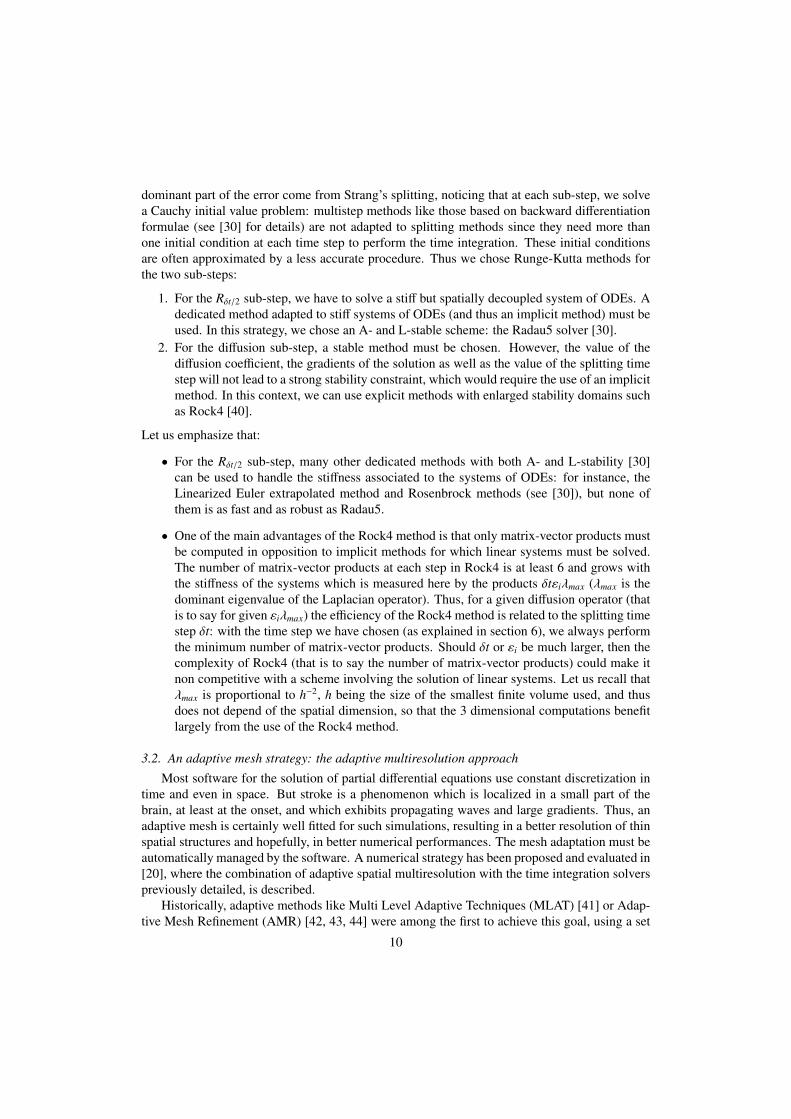
3.2. An adaptive mesh strategy: the adaptive multiresolution approach
Most software for the solution of partial differential equations use constant discretization intime and even in space. But stroke is a phenomenon which is localized in a small part of thebrain, at least at the onset, and which exhibits propagating waves and large gradients. Thus, anadaptive mesh is certainly well fitted for such simulations, resulting in a better resolution of thinspatial structures and hopefully, in better numerical performances. The mesh adaptation must beautomatically managed by the software. A numerical strategy has been proposed and evaluated in[20], where the combination of adaptive spatial multiresolution with the time integration solverspreviously detailed, is described.
Historically, adaptive methods like Multi Level Adaptive Techniques (MLAT) [41] or Adap-tive Mesh Refinement (AMR) [42, 43, 44] were among the first to achieve this goal, using a set
10
of locally refined grids where steep gradients are found. Furthermore, adaptive multiresolutionmethods, based on Harten’s pioneering work [45], have been developed for 1D and 2D hyper-bolic conservation laws [46, 47] and then extended to 3D parabolic problems [48]. Consequently,high data compression might be achieved with all these methods. However, one major advantageof the adaptive multiresolution techniques is that the numerical analysis of the errors has alreadybeen conducted [45, 46] and thus, a solid theoretical background has already been settled.
λ0Ω Ω=
j =
j
j
j
j
=
=
=
=
2
1
...
0
J
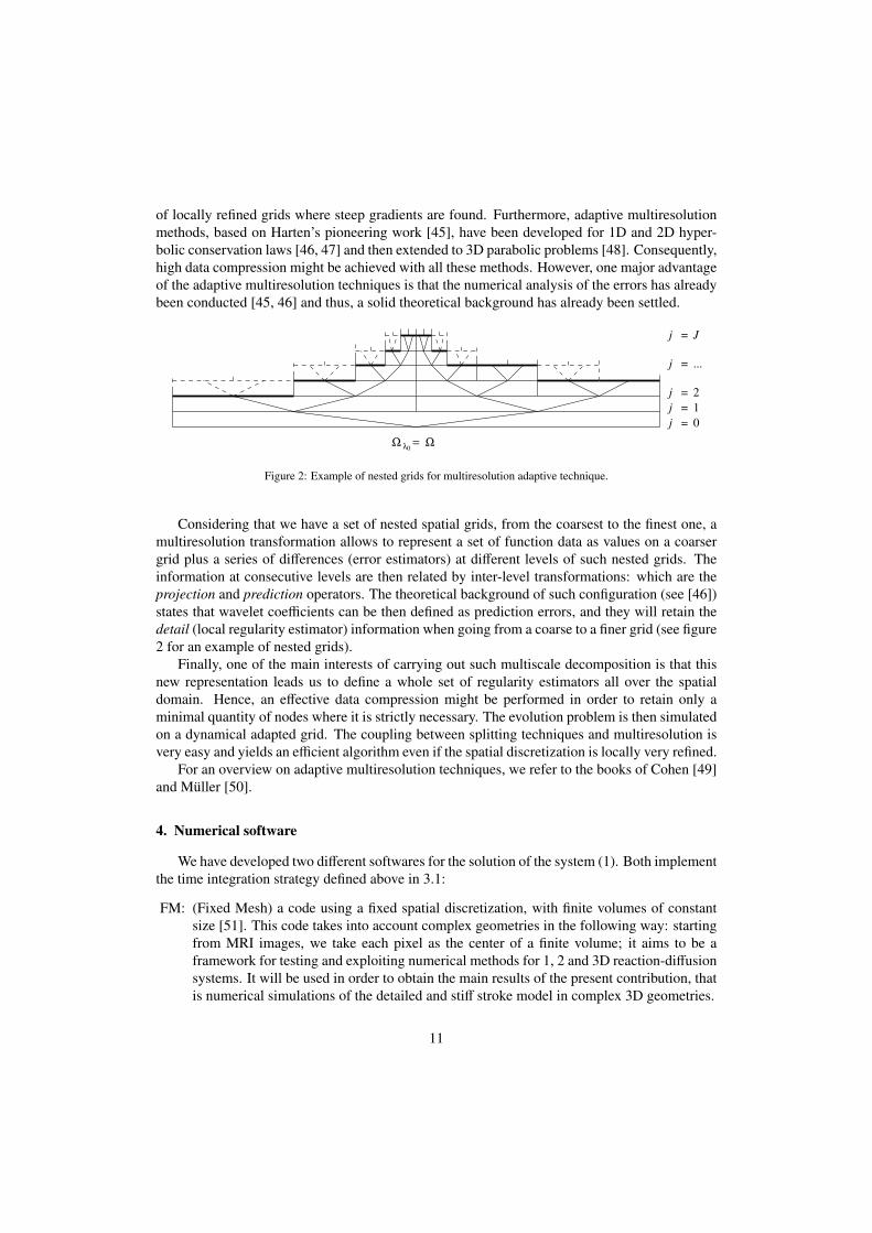
Figure 2: Example of nested grids for multiresolution adaptive technique.
Considering that we have a set of nested spatial grids, from the coarsest to the finest one, amultiresolution transformation allows to represent a set of function data as values on a coarsergrid plus a series of differences (error estimators) at different levels of such nested grids. Theinformation at consecutive levels are then related by inter-level transformations: which are theprojection and prediction operators. The theoretical background of such configuration (see [46])states that wavelet coefficients can be then defined as prediction errors, and they will retain thedetail (local regularity estimator) information when going from a coarse to a finer grid (see figure2 for an example of nested grids).
Finally, one of the main interests of carrying out such multiscale decomposition is that thisnew representation leads us to define a whole set of regularity estimators all over the spatialdomain. Hence, an effective data compression might be performed in order to retain only aminimal quantity of nodes where it is strictly necessary. The evolution problem is then simulatedon a dynamical adapted grid. The coupling between splitting techniques and multiresolution isvery easy and yields an efficient algorithm even if the spatial discretization is locally very refined.
For an overview on adaptive multiresolution techniques, we refer to the books of Cohen [49]and Muller [50].
4. Numerical software
We have developed two different softwares for the solution of the system (1). Both implementthe time integration strategy defined above in 3.1:
FM: (Fixed Mesh) a code using a fixed spatial discretization, with finite volumes of constantsize [51]. This code takes into account complex geometries in the following way: startingfrom MRI images, we take each pixel as the center of a finite volume; it aims to be aframework for testing and exploiting numerical methods for 1, 2 and 3D reaction-diffusionsystems. It will be used in order to obtain the main results of the present contribution, thatis numerical simulations of the detailed and stiff stroke model in complex 3D geometries.
11
MR: (Multi Resolution) a code using an adaptive multiresolution method as defined above in3.2. In the framework of multiresolution, an important amount of work is still requiredin order to optimally combine all the numerical methods described here, the most difficultaspects are related to programming features such as data and code structures, as indicatedin [20]. Nowadays, this program can only solve problems in simple domains like squaresand cubes; simulations with an adaptive multiresolution approach on a complex geometryare not yet available, and we will only present here 2D and 3D simulations in simplifiedgeometries for the sake of assessing our results and perspectives in the field.
Let us remark that the (FM) code is a highly optimized and complete code for the simula-tion of reaction-diffusion equations. In particular, stroke simulations in complex geometry canbe performed for the first time, with standard computing resources, and constitutes the majoradvance of our contribution. On the other hand, the second code (MR) allows to validate to someextents the previous numerical results, and it is meant to be a potential extension to (FM) infuture developments.
5. Implementation and performances of the numerical methods on shared memory ma-chines
We describe now the implementation of the 3D simulations which are performed on a uni-form grid and a complex geometry with the code (FM). Let us emphasize the particular paral-lelism implementation that we have conceived in the framework of shared memory machines.All the computations have been performed on a 8 core (2x4) 64 bits machine (AMD Shanghaiprocessors).
Since an implicit procedure is required to handle the associated stiffness, the reaction stepsare by far the most time consuming parts of the computation. This step is naturally parallel, aswe have to solve a large number ` of independent systems of differential equations, each of themcorresponding to a single cell. But solvers like Radau5 use a time adaptive strategy, togetherwith Newton method: that is, the computing time is varying from one point to another, and afixed domain partition strategy, with an affectation of sub-domains to processors, is not optimalfor load balancing. Therefore, our implementation uses threads, implemented in the C++ boost-thread library [52]. Let us describe it shortly in the next part.
We divide the set of finite volumes into small subsets S i, i = 1, ..., k where k should bemuch larger than the number of computing units. We build a stack of all the S i before each timestep. By calling the procedure GetSubset, each thread gets one S i, while the stack is not empty.Threads join when the stack is empty.
12
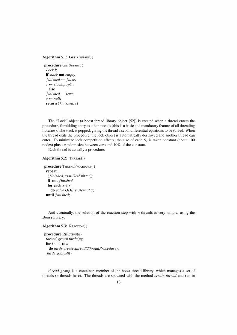
Algorithm 5.1: Get a subset( )
procedure GetSubset( )Lock l;if stack not emptyf inished ← f alse;s← stack.pop();
elsef inished ← true;s← null;return ( f inished, s)
The “Lock” object (a boost thread library object [52]) is created when a thread enters theprocedure, forbidding entry to other threads (this is a basic and mandatory feature of all threadinglibraries). The stack is popped, giving the thread a set of differential equations to be solved. Whenthe thread exits the procedure, the lock object is automatically destroyed and another thread canenter. To minimize lock competition effects, the size of each S i is taken constant (about 100nodes) plus a random size between zero and 10% of the constant.
Each thread is actually a procedure:
Algorithm 5.2: Thread( )
procedure ThreadProcedure( )repeat( f inished, s) = GetS ubset();if not f inishedfor each x ∈ s
do solve ODE system at x;until f inished;
And eventually, the solution of the reaction step with n threads is very simple, using theBoost library:
Algorithm 5.3: Reaction( )
procedure Reaction(n)thread group thrds(n);for i← 1 to n
do thrds.create thread(ThreadProcedure);thrds. join all()
thread group is a container, member of the boost-thread library, which manages a set ofthreads (n threads here). The threads are spawned with the method create thread and run in
13
parallel, each thread launching the ThreadProcedure routine. The join all method acts as ameeting point for all the threads, and the execution waits until all threads have finished theircomputations.
6. Numerical results: implementation checkout and accuracy evaluation of the code
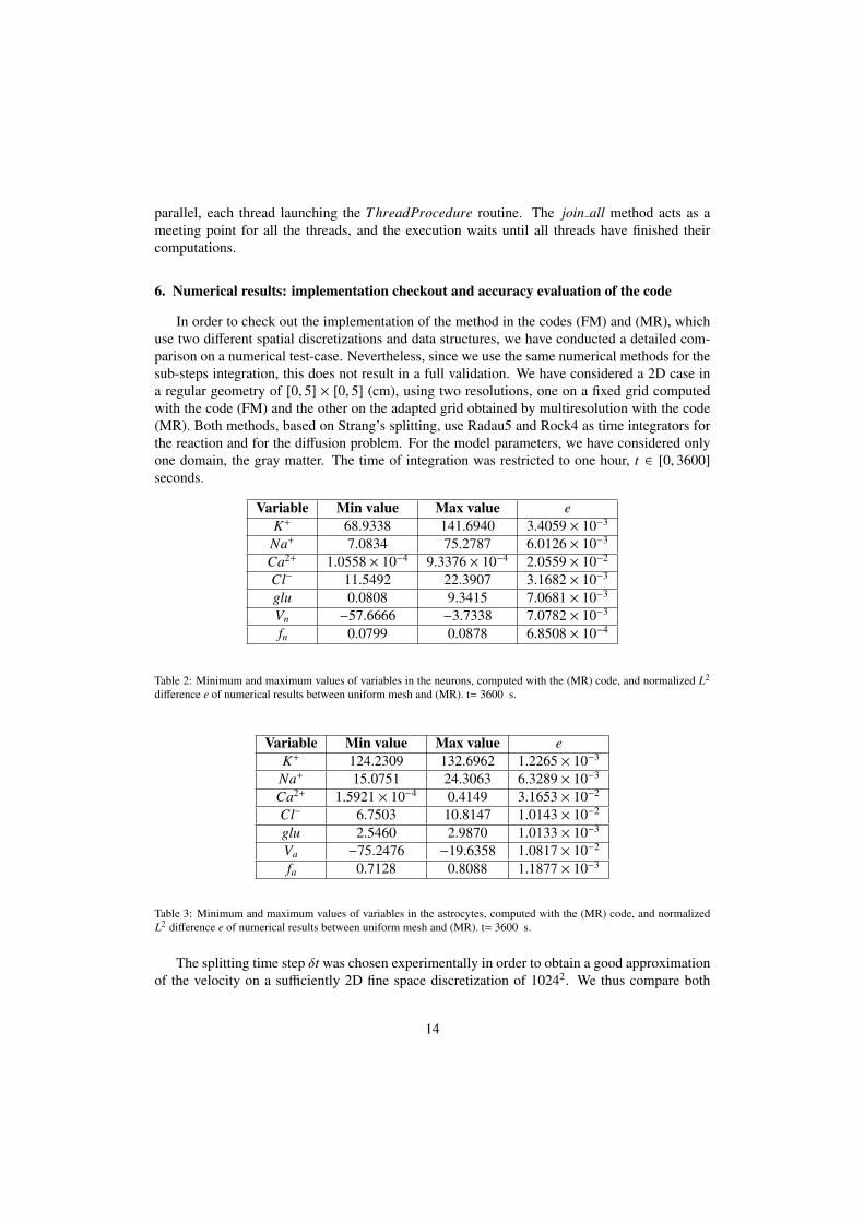
In order to check out the implementation of the method in the codes (FM) and (MR), whichuse two different spatial discretizations and data structures, we have conducted a detailed com-parison on a numerical test-case. Nevertheless, since we use the same numerical methods for thesub-steps integration, this does not result in a full validation. We have considered a 2D case ina regular geometry of [0, 5] × [0, 5] (cm), using two resolutions, one on a fixed grid computedwith the code (FM) and the other on the adapted grid obtained by multiresolution with the code(MR). Both methods, based on Strang’s splitting, use Radau5 and Rock4 as time integrators forthe reaction and for the diffusion problem. For the model parameters, we have considered onlyone domain, the gray matter. The time of integration was restricted to one hour, t ∈ [0, 3600]seconds.
Variable Min value Max value eK+ 68.9338 141.6940 3.4059 × 10⁻³
Na+ 7.0834 75.2787 6.0126 × 10⁻³
Ca2+ 1.0558 × 10⁻⁴ 9.3376 × 10⁻⁴ 2.0559 × 10⁻²
Cl− 11.5492 22.3907 3.1682 × 10⁻³
glu 0.0808 9.3415 7.0681 × 10⁻³
Vn −57.6666 −3.7338 7.0782 × 10⁻³
fn 0.0799 0.0878 6.8508 × 10⁻⁴
Table 2: Minimum and maximum values of variables in the neurons, computed with the (MR) code, and normalized L2
difference e of numerical results between uniform mesh and (MR). t= 3600 s.
Variable Min value Max value eK+ 124.2309 132.6962 1.2265 × 10⁻³
Na+ 15.0751 24.3063 6.3289 × 10⁻³
Ca2+ 1.5921 × 10⁻⁴ 0.4149 3.1653 × 10⁻²
Cl− 6.7503 10.8147 1.0143 × 10⁻²
glu 2.5460 2.9870 1.0133 × 10⁻³
Va −75.2476 −19.6358 1.0817 × 10⁻²
fa 0.7128 0.8088 1.1877 × 10⁻³
Table 3: Minimum and maximum values of variables in the astrocytes, computed with the (MR) code, and normalizedL2 difference e of numerical results between uniform mesh and (MR). t= 3600 s.
The splitting time step δt was chosen experimentally in order to obtain a good approximationof the velocity on a sufficiently 2D fine space discretization of 10242. We thus compare both
14
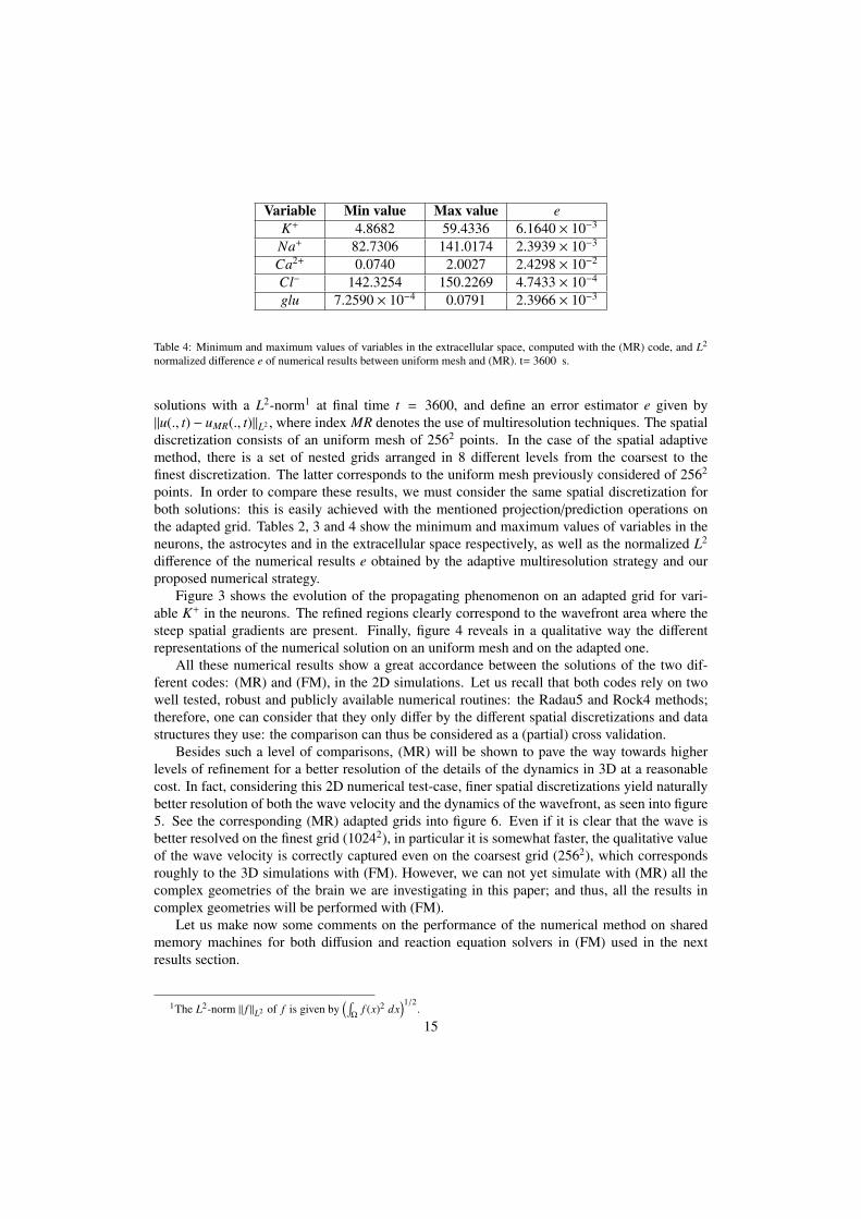
Variable Min value Max value eK+ 4.8682 59.4336 6.1640 × 10⁻³
Na+ 82.7306 141.0174 2.3939 × 10⁻³
Ca2+ 0.0740 2.0027 2.4298 × 10⁻²
Cl− 142.3254 150.2269 4.7433 × 10⁻⁴
glu 7.2590 × 10⁻⁴ 0.0791 2.3966 × 10⁻³
Table 4: Minimum and maximum values of variables in the extracellular space, computed with the (MR) code, and L2
normalized difference e of numerical results between uniform mesh and (MR). t= 3600 s.
solutions with a L2-norm1 at final time t = 3600, and define an error estimator e given by‖u(., t) − uMR(., t)‖L2 , where index MR denotes the use of multiresolution techniques. The spatialdiscretization consists of an uniform mesh of 2562 points. In the case of the spatial adaptivemethod, there is a set of nested grids arranged in 8 different levels from the coarsest to thefinest discretization. The latter corresponds to the uniform mesh previously considered of 2562
points. In order to compare these results, we must consider the same spatial discretization forboth solutions: this is easily achieved with the mentioned projection/prediction operations onthe adapted grid. Tables 2, 3 and 4 show the minimum and maximum values of variables in theneurons, the astrocytes and in the extracellular space respectively, as well as the normalized L2
difference of the numerical results e obtained by the adaptive multiresolution strategy and ourproposed numerical strategy.
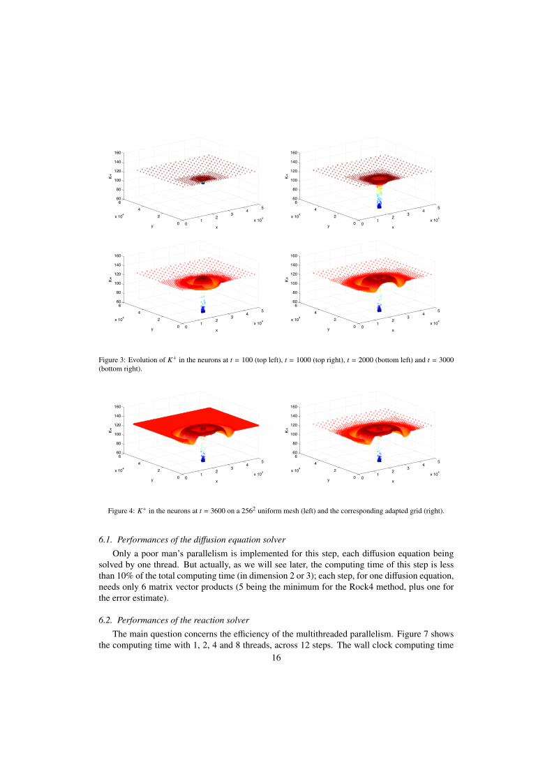
Figure 3 shows the evolution of the propagating phenomenon on an adapted grid for vari-able K+ in the neurons. The refined regions clearly correspond to the wavefront area where thesteep spatial gradients are present. Finally, figure 4 reveals in a qualitative way the differentrepresentations of the numerical solution on an uniform mesh and on the adapted one.
All these numerical results show a great accordance between the solutions of the two dif-ferent codes: (MR) and (FM), in the 2D simulations. Let us recall that both codes rely on twowell tested, robust and publicly available numerical routines: the Radau5 and Rock4 methods;therefore, one can consider that they only differ by the different spatial discretizations and datastructures they use: the comparison can thus be considered as a (partial) cross validation.
Besides such a level of comparisons, (MR) will be shown to pave the way towards higherlevels of refinement for a better resolution of the details of the dynamics in 3D at a reasonablecost. In fact, considering this 2D numerical test-case, finer spatial discretizations yield naturallybetter resolution of both the wave velocity and the dynamics of the wavefront, as seen into figure5. See the corresponding (MR) adapted grids into figure 6. Even if it is clear that the wave isbetter resolved on the finest grid (10242), in particular it is somewhat faster, the qualitative valueof the wave velocity is correctly captured even on the coarsest grid (2562), which correspondsroughly to the 3D simulations with (FM). However, we can not yet simulate with (MR) all thecomplex geometries of the brain we are investigating in this paper; and thus, all the results incomplex geometries will be performed with (FM).
Let us make now some comments on the performance of the numerical method on sharedmemory machines for both diffusion and reaction equation solvers in (FM) used in the nextresults section.
1The L2-norm ‖ f ‖L2 of f is given by(∫
Ωf (x)2 dx
)1/2.
15
01
23
45
x 104
02
46
x 104
60
80
100
120
140
160
xy
K+
01
23
45
x 104
02
46
x 104
60
80
100
120
140
160
xy
K+
01
23
45
x 104
02
46
x 104
60
80
100
120
140
160
xy
K+
01
23
45
x 104
02
46
x 104
60
80
100
120
140
160
xy
K+
Figure 3: Evolution of K+ in the neurons at t = 100 (top left), t = 1000 (top right), t = 2000 (bottom left) and t = 3000(bottom right).
01
23
45
x 104
02
46
x 104
60
80
100
120
140
160
xy
K+
01
23
45
x 104
02
46
x 104
60
80
100
120
140
160
xy
K+
Figure 4: K+ in the neurons at t = 3600 on a 2562 uniform mesh (left) and the corresponding adapted grid (right).
6.1. Performances of the diffusion equation solver
Only a poor man’s parallelism is implemented for this step, each diffusion equation beingsolved by one thread. But actually, as we will see later, the computing time of this step is lessthan 10% of the total computing time (in dimension 2 or 3); each step, for one diffusion equation,needs only 6 matrix vector products (5 being the minimum for the Rock4 method, plus one forthe error estimate).
6.2. Performances of the reaction solver
The main question concerns the efficiency of the multithreaded parallelism. Figure 7 showsthe computing time with 1, 2, 4 and 8 threads, across 12 steps. The wall clock computing time
16
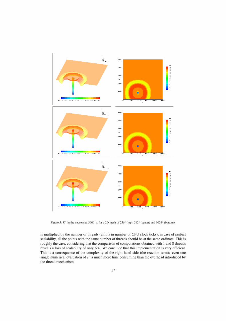
Figure 5: K+ in the neurons at 3600 s. for a 2D mesh of 2562 (top), 5122 (center) and 10242 (bottom).
is multiplied by the number of threads (unit is in number of CPU clock ticks); in case of perfectscalability, all the points with the same number of threads should be at the same ordinate. This isroughly the case, considering that the comparison of computations obtained with 1 and 8 threadsreveals a loss of scalability of only 6%. We conclude that this implementation is very efficient.This is a consequence of the complexity of the right hand side (the reaction term): even onesingle numerical evaluation of F is much more time consuming than the overhead introduced bythe thread mechanism.
17

Figure 6: 2D adapted meshes equivalent to 2562 (left) and 10242 (right) spatial discretizations at the finest grid.
As a conclusion of this part, we can notice that our computing strategy combining splittingtechniques with dedicated integration of each sub-step and multiresolution is compatible withparallelization.
Figure 7: Performances of the multithreaded reaction solver along 12 time steps. Abscissa: time step. Ordinate: com-puting time in CPU clock ticks.
7. Biological results
We present and discuss here some simulation results obtained with the code FM on the com-plex geometry of the human brain. We simulate an ischemic stroke beginning in the cortex (ingray matter) and study the propagation of the ischemic damage. The input of the model is the
18
decrease of the ionic currents through the ionic pumps. Two variables have been chosen for themodel validation: the potassium concentration in the extracellular space ([K+]e) and the ratio ofapparent diffusion coefficient of water (rADCw).
• The potassium concentration cannot be measured in vivo in the brain of stroke patientsbut it can be measured ex vivo or in vitro on brain tissues. These concentration valuesgive some insights on the severity of the damage. The physiological value of [K+]e isabout 5 mM. It was observed to be able to increase up to 35 mM in areas of moderateischemia where depolarization waves can spread [53] and up to 75-90 mM in areas ofsevere ischemia where most cells are dead [54]. The first step of the model validation isthus to compare the values of the [K+]e obtained in the simulations with those values.
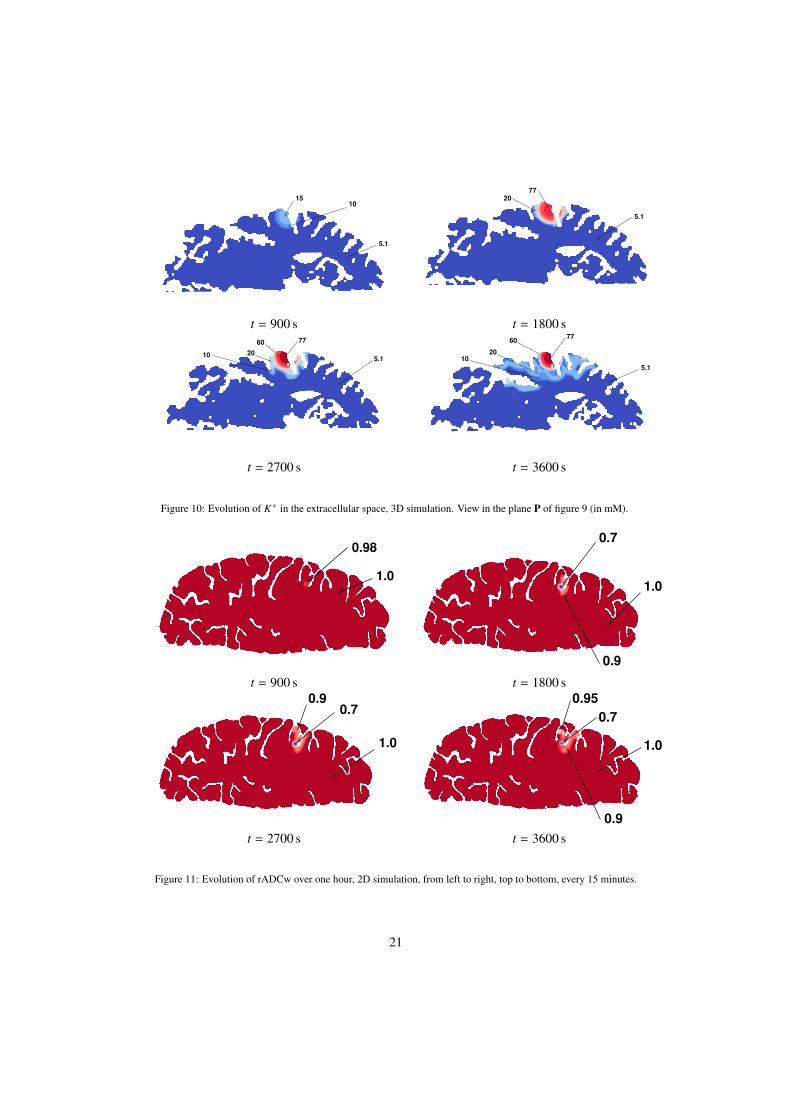
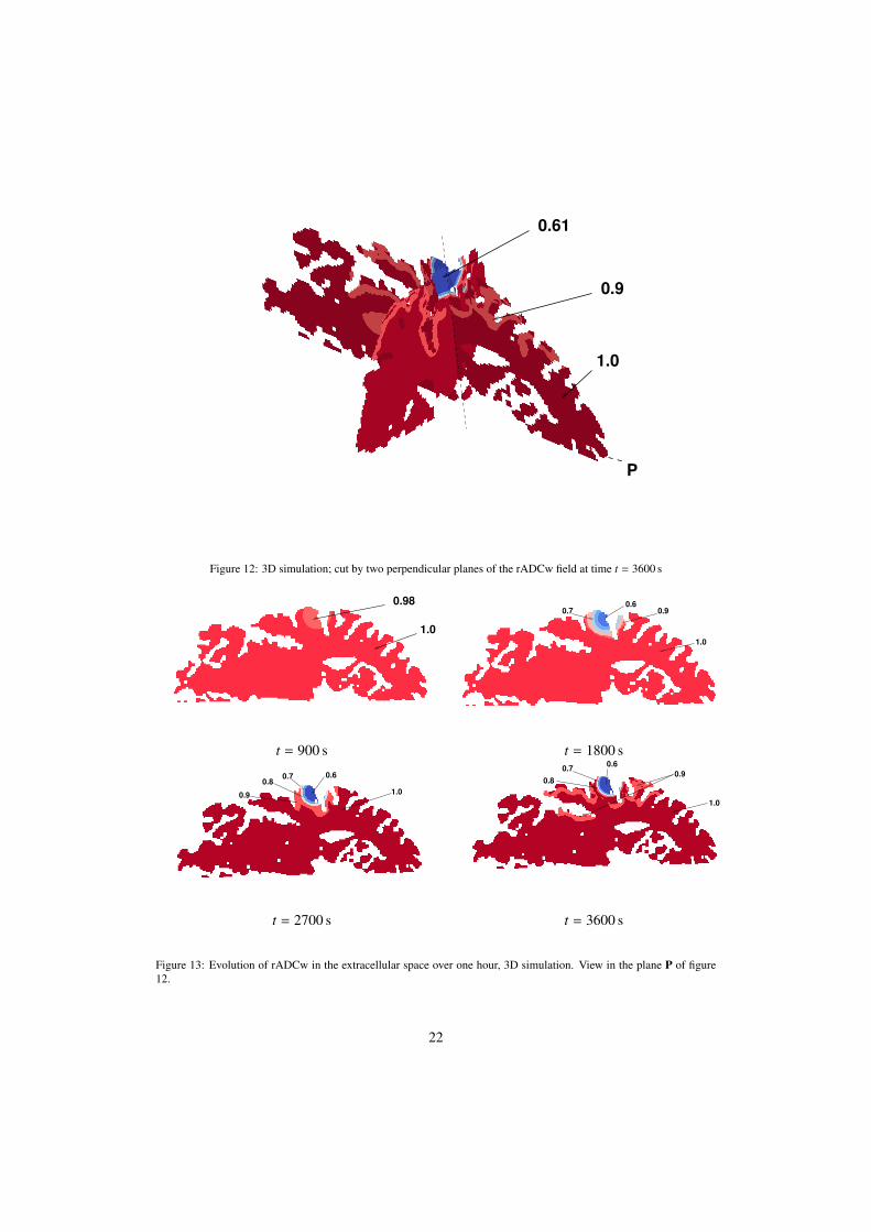
• The rADCw is a biomarker which can be estimated in the brain of stroke patients thanksto diffusion-weighted (DW) magnetic resonance (MRI) imaging. It reflects the severityof the cytotoxic edema and could thus be used to predict the ischemic damage and itsextension [55, 56]. The value of this ratio is supposed to be 1 in physiological conditionsand is known to decrease in ischemic areas. In several studies, this value in stroke patientswas shown to be between 0.75 and 0.9 in areas of moderate ischemia and between 0.5 and0.75 in areas of severe ischemia [57, 58, 59, 60]. This biomarker can be related to theproportions of the intracellular volumes. It was shown to be proportional to the volume ofthe extracellular space [55]. Moreover, since the extracellular proportion was displayed tohave a value of 0.2 in physiological conditions (i.e. when rADCw=1) [61], rADCw canbe expressed as follows: rADCw = 5 (1 − fn − fa). Since fn and fa are two variables ofthe model, this ratio can be calculated for each time and for each coordinate. Another stepof the model validation is thus to compare the calculated values of rADCw obtained in thesimulations to the experimental values.
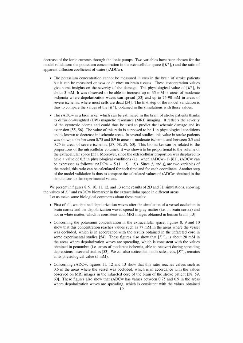
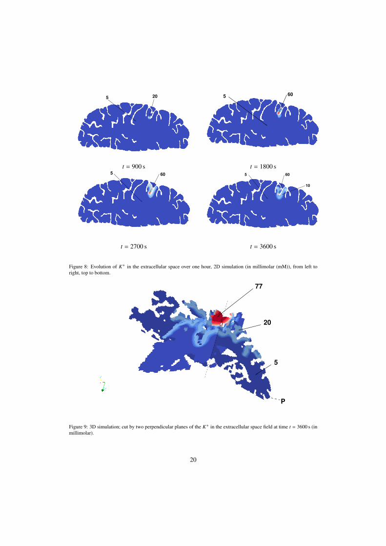
We present in figures 8, 9, 10, 11, 12, and 13 some results of 2D and 3D simulations, showingthe values of K+ and rADCw biomarker in the extracellular space in different areas.
Let us make some biological comments about these results:
• First of all, we obtained depolarization waves after the simulation of a vessel occlusion inbrain cortex and the depolarization waves spread in gray matter (i.e. in brain cortex) andnot in white matter, which is consistent with MRI images obtained in human brain [13].
• Concerning the potassium concentration in the extracellular space, figures 8, 9 and 10show that this concentration reaches values such as 77 mM in the areas where the vesselwas occluded, which is in accordance with the results obtained in the infarcted core insome experimental studies [54]. These figures also show that [K+]e is about 20 mM inthe areas where depolarization waves are spreading, which is consistent with the valuesobtained in penumbra (i.e. areas of moderate ischemia, able to recover) during spreadingdepressions in several studies [53]. We can also notice that, in the safe areas, [K+]e remainsat its physiological value (5 mM).
• Concerning rADCw, figures 11, 12 and 13 show that this ratio reaches values such as0.6 in the areas where the vessel was occluded, which is in accordance with the valuesobserved on MRI images in the infarcted core of the brain of the stroke patient [58, 59,60]. These figures also show that rADCw has values between 0.75 and 0.9 in the areaswhere depolarization waves are spreading, which is consistent with the values obtained
19
5 20 560
t = 900 s t = 1800 s605
10
605
t = 2700 s t = 3600 s
Figure 8: Evolution of K+ in the extracellular space over one hour, 2D simulation (in millimolar (mM)), from left toright, top to bottom.
20
5
77
P
Figure 9: 3D simulation; cut by two perpendicular planes of the K+ in the extracellular space field at time t = 3600 s (inmillimolar).
20
5.1
1015
5.1
20
77
t = 900 s t = 1800 s
5.110 20
60 77
5.1
7760
20
10
t = 2700 s t = 3600 s
Figure 10: Evolution of K+ in the extracellular space, 3D simulation. View in the plane P of figure 9 (in mM).
1.0
0.980.7
1.0
0.9
t = 900 s t = 1800 s
1.0
0.70.9
0.9
0.95
0.7
1.0
t = 2700 s t = 3600 s
Figure 11: Evolution of rADCw over one hour, 2D simulation, from left to right, top to bottom, every 15 minutes.
21
0.9
0.61
1.0
P
Figure 12: 3D simulation; cut by two perpendicular planes of the rADCw field at time t = 3600 s
1.0
0.980.7
0.60.9
1.0
t = 900 s t = 1800 s
0.9
0.80.7 0.6
1.0
1.0
0.9
0.60.7
0.8
t = 2700 s t = 3600 s
Figure 13: Evolution of rADCw in the extracellular space over one hour, 3D simulation. View in the plane P of figure12.
22
in penumbra during spreading depressions in stroke patients [58, 60]. We can also noticethat, in the safe areas, rADCw remains at its physiological value of 1.
To conclude, the simulation results concerning the localization of spreading depressions andthe values of [K+]e and rADCw are consistent with those obtained in experimental studies orobserved on MRI images in stroke patients. These results give thus a first step of validation forthe model and for the numerical methods used in this study.
8. Toward better computational efficiency and improved accuracy: Adaptive Multiresolu-tion
In the previous simulations, we notice that the simulated waves spread at a slightly slowerspeed. In several studies, spreading depressions were shown to spread at a rate of several mil-limeters per minute [62], which is not currently the case in our simulations. In fact, it is shown in[63] that traveling waves solutions of reaction–diffusion equations can disappear in the numericalsolution if the spatial discretization is too coarse; the velocity of the traveling waves is a functionof the mesh size, and coarse meshes might perturb the accuracy of the computed wave velocity.In particular, in the previous 3D simulations, the mesh we can use is not fine enough to obtain acorrect level of accuracy for the wave velocities. In fact, coming back to the 2D numerical test-case of section 6, we have seen in figure 5, that a high number of volumes is needed to reproduceaccurately the phenomenon, approximately 1000 per dimension.
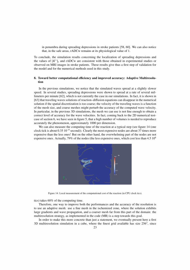
We can also measure the computing time of the reaction at a typical step (see figure 14 (oneclock tick is about 0.35 10−9 second)). Clearly the most expensive nodes are about 37 times moreexpensive than the less ones! But on the other hand, the overwhelming part of the nodes are notexpensive ones. Actually, 79% of the nodes (the less expensive ones, which cost less than 4.5 106
Figure 14: Local measurement of the computational cost of the reaction (in CPU clock tics).
tics) takes 60% of the computing time.Therefore, one way to improve both the performances and the accuracy of the resolution is
to use an adaptive mesh: use a fine mesh in the ischemized zone, where the solution exhibitslarge gradients and wave propagation, and a coarser mesh far from this part of the domain: themultiresolution strategy, as implemented in the code (MR) is a step towards this goal.
In order to make this more concrete than just a statement, we eventually present here a first3D multiresolution simulation in a cube, where the finest grid available has size 2563, since
23
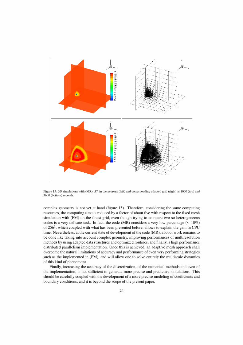
Figure 15: 3D simulations with (MR). K+ in the neurons (left) and corresponding adapted grid (right) at 1000 (top) and3600 (bottom) seconds.
complex geometry is not yet at hand (figure 15). Therefore, considering the same computingresources, the computing time is reduced by a factor of about five with respect to the fixed meshsimulation with (FM) on the finest grid, even though trying to compare two so heterogeneouscodes is a very delicate task. In fact, the code (MR) considers a very low percentage (≤ 10%)of 2563, which coupled with what has been presented before, allows to explain the gain in CPUtime. Nevertheless, at the current state of development of the code (MR), a lot of work remains tobe done like taking into account complex geometry, improving performances of multiresolutionmethods by using adapted data structures and optimized routines, and finally, a high performancedistributed parallelism implementation. Once this is achieved, an adaptive mesh approach shallovercome the natural limitations of accuracy and performance of even very performing strategiessuch as the implemented in (FM), and will allow one to solve entirely the multiscale dynamicsof this kind of phenomena.
Finally, increasing the accuracy of the discretization, of the numerical methods and even ofthe implementation, is not sufficient to generate more precise and predictive simulations. Thisshould be carefully coupled with the development of a more precise modeling of coefficients andboundary conditions, and it is beyond the scope of the present paper.
24
9. Conclusions and future work
We have presented for the first time numerical 3D simulations of an ischemic stroke in arealistic brain geometry, based on the model of Dronne et al. [9]. Results are encouraging fromnumerical and medical points of view. This is a first major step towards an usable tool for pre-dicting the evolution of a stroke. The next steps are to improve both numerical performances andmodeling. For this, a lot of work remains to be done from the model to practical implementa-tions. Concerning the numerical methods, many parameters in the model are known only with acoarse approximation. Thus, numerical simulations must be conducted to explore the sensitivityof the model to these parameters. The ultimate way to improve the performances is to switchfrom multithreaded parallelism to distributed parallelism, on massive parallel computers.
From a medical point of view, this model is of the most importance since it could be used tosimulate on a realistic human brain geometry several neuroprotective agents aimed at blockingthe ischemic cascade and at reducing the ischemic damage. Since the model contains manypharmacological targets (such as ionic transporters, voltage-gated channels, channel-receptorsand stretch channels), it could be used to assess and study the effects of various therapeutic agentsor associations of therapeutic agents. Moreover, since the model includes both ionic movementsthrough the cells and their diffusion, we will be able to study the effects of these neuroprotectiveagents both on the severity and on the extension of the damage in each brain area. Developingpowerful numerical methods are thus of the most importance to be able to simulate the time andspatial evolutions of these phenomena on a realistic human brain geometry.
Acknowledgments
This research was supported by two ANR grants (Agence Nationale pour la Recherche -French National Research Agency): AVC in silico (ANR-06-BYOS-0002-02 - projects leaders:M.-A. Dronne and E. Grenier - 2006-2009) and Sechelles (ANR-09-BLAN-0075-01 - projectleader: S. Descombes - 2009-2013). We would like to thank Christian Tenaud (LIMSI - CNRS)for providing the basis of the multiresolution kernel of MR CHORUS, code that he developed atLIMSI for compressible Navier-Stokes equations.
References
[1] D. Lloyd-Jones, R. Adams, M. Carnethon, G. De Simone, T. B. Ferguson, K. Flegal, E. Ford, K. Furie, A. Go,K. Greenlund, N. Haase, S. Hailpern, M. Ho, V. Howard, B. Kissela, S. Kittner, D. Lackland, L. Lisabeth,A. Marelli, M. McDermott, J. Meigs, D. Mozaffarian, G. Nichol, C. O’Donnell, V. Roger, W. Rosamond, R. Sacco,P. Sorlie, R. Stafford, J. Steinberger, T. Thom, S. Wasserthiel-Smoller, N. Wong, J. Wylie-Rosett, Y. Hong, Heartdisease and stroke statistics–2009 update: A report from the American Heart Association Statistics Committee andStroke Statistics Subcommittee, Circulation 119 (3) (2009) e21–181.
[2] U. Dirnagl, C. Iadecola, M. Moskowitz, Pathobiology of ischaemic stroke: an integrated view, Trends in Neuro-sciences 22 (9) (1999) 391–397.
[3] M. A. Moskowitz, E. H. Lo, C. Iadecola, The science of stroke: mechanisms in search of treatments, Neuron 67 (2)(2010) 181–198.
[4] G. D. Graham, Tissue plasminogen activator for acute ischemic stroke., Stroke 34 (2003) 2847–2850.[5] J. De Keyser, G. Sulter, P. Luiten, Clinical trials with neuroprotective drugs in acute ischaemic stroke: are we doing
the right thing?, Trends in Neurosciences 22 (12) (1999) 535–40.[6] P. A. Barber, R. N. Auer, A. M. Buchan, G. R. Sutherland, Understanding and managing ischemic stroke, Can. J.
Physiol. Pharmacol. 79 (3) (2001) 283–296.[7] N. G. Wahlgren, N. Ahmed, Neuroprotection in cerebral ischaemia: facts and fancies–the need for new approaches,
Cerebrovasc. Dis. 17 (2004) 155–166.
25
[8] A. Durukan, T. Tatlisumak, Acute ischemic stroke: Overview of major experimental rodent models, pathophysiol-ogy, and therapy of focal cerebral ischemia, Pharmacology Biochemistry and Behavior 87 (1) (2007) 179–197.
[9] M.-A. Dronne, J.-P. Boissel, E. Grenier, A mathematical model of ion movements in grey matter during a stroke, J.of Theoretical Biology 240 (4) (2006) 599–615.
[10] M.-A. Dronne, E. Grenier, T. Dumont, M. Hommel, J.-P. Boissel, Role of astrocytes in grey matter during a stroke:A modelling approach, Brain Research 1138 (2007) 231–242.
[11] M.-A. Dronne, S. Descombes, E. Grenier, H. Gilquin, Examples of the influence of the geometry on the propagationof progressive waves, Math. Comput. Modelling 49 (11-12) (2009) 2138–2144, ISSN 0895-7177.
[12] G. G. Somjen, Mechanisms of spreading depression and hypoxic spreading depression-like depolarization, Physiol.Rev. 81 (3).
[13] C. Dohmen, O. W. Sakowitz, M. Fabricius, B. Bosche, T. Reithmeier, R.-I. Ernestus, G. Brinker, J. P. Dreier,J. Woitzik, A. J. Strong, R. Graf, Spreading depolarizations occur in human ischemic stroke with high incidence,Annals of Neurology 63 (2008) 720–728.
[14] H. K. Shin, A. K. Dunn, P. B. Jones, D. A. Boas, M. A. Moskowitz, C. Ayata, Vasoconstrictive neurovascularcoupling during focal ischemic depolarizations, J. Cereb. Blood Flow & Metab. 26 (8) (2005) 1018–1030.
[15] K. Revett, E. Ruppin, S. Goodall, J. A. Reggia, Spreading depression in focal ischemia: a computational study, J.Cereb. Blood Flow & Metab. 18 (9) (1998) 998–1007.
[16] H. Kager, W. J. Wadman, G. G. Somjen, Simulated seizures and spreading depression in a neuron model incorpo-rating interstitial space and ion concentrations, J. Neurophysiol. 84 (1) (2000) 495–512.
[17] M.-A. Dronne, E. Grenier, G. Chapuisat, M. Hommel, J.-P. Boissel, A modelling approach to explore some hy-potheses of the failure of neuroprotective trials in ischemic stroke patient, Progress in Biophysics & MolecularBiology 97 (2008) 60–78.
[18] E. Grenier, M.-A. Dronne, S. Descombes, H. Gilquin, A. Jaillard, M. Hommel, J.-P. Boissel, A numerical study ofthe blocking of migraine by Rolando sulcus, Progress in Biophysics & Molecular Biology 97 (1) (2008) 54–59.
[19] S. Descombes, T. Dumont, Numerical simulation of a stroke: Computational problems and methodology, Progressin Biophysics & Molecular Biology 97 (1) (2008) 40–53.
[20] M. Duarte, M. Massot, S. Descombes, C. Tenaud, T. Dumont, V. Louvet, F. Laurent, New resolution strategy formulti-scale reaction waves using time operator splitting, space adaptive multiresolution and dedicated high orderimplicit/explicit time integrators, SIAM J. Sci. Comput. 34 (1) (2012) A76–A104.
[21] A. L. Hodgkin, A. F. Huxley, A quantitative description of membrane current and its application to conduction andexcitation in nerve, J. Physiol. 117 (4) (1952) 500–544.
[22] W. Walz, Role of Na/K/Cl cotransport in astrocytes, Can. J. Physiol. Pharmacol 70 (1992) S260–S262.[23] A. Destexhe, Z. Mainen, T. Sejnowski, Kinetic models of synaptic transmission, chap. 1, MIT Press,Cambridge,
MA, 1998.[24] W. Yamada, C. Koch, P. Adams, Methods in Neuronal Modeling: From Ions to Networks, chap. 1, MIT Press,
Cambridge, MA, 137–170, 1998.[25] D. Rossi, T. Oshima, D. Attwell, Glutamate release in severe brain ischaemia is mainly by reversed uptake, Nature
403 (2000) 316–321.[26] B. Shapiro, Osmotic forces and gap junctions in spreading depression: a computational model, J. Comput. Neu-
rosci. 10 (2001) 877–896.[27] D. DiFrancesco, D. Noble, A model of cardiac electrical activity incorporating ionic pumps and concentration
changes, Philos. Trans. R. Soc. Lond. B Biol. Sci. 307 (1133) (1985) 353–398.[28] D. Lemieux, F. Roberge, D. Joly, Modeling the dynamic features of the electrogenic Na,K pump of cardiac cells,
J. Theor. Biol. 3 (1992) 335–358.[29] C. Yi, A. Fogelson, J. Keener, C. Peskin, A mathematical study of volume shifts and ionic concentration changes
during ischemia and hypoxia., J Theor Biol. 220 (1) (2003) 83–106.[30] E. Hairer, G. Wanner, Solving ordinary differential equations. II, vol. 14 of Springer Series in Computational
Mathematics, Springer-Verlag, Berlin, second edn., stiff and differential-algebraic problems, 1996.[31] G. Akrivis, M. Crouzeix, C. Makridakis, Implicit-explicit multistep finite element methods for nonlinear parabolic
problems, Math. Comp. 67 (222) (1998) 457–477.[32] B. P. Sommeijer, L. F. Shampine, J. G. Verwer, RKC: an explicit solver for parabolic PDEs, J. Comput. Appl. Math.
88 (2) (1998) 315–326.[33] J. G. Verwer, B. P. Sommeijer, An implicit-explicit Runge-Kutta-Chebyshev scheme for diffusion-reaction equa-
tions, SIAM J. Sci. Comput. 25 (5) (2004) 1824–1835 (electronic).[34] J. G. Verwer, B. P. Sommeijer, W. Hundsdorfer, RKC time-stepping for advection-diffusion-reaction problems, J.
Comput. Phys. 201 (1) (2004) 61–79.[35] L. F. Shampine, B. P. Sommeijer, J. G. Verwer, IRKC: an IMEX solver for stiff diffusion-reaction PDEs, J. Comput.
Appl. Math. 196 (2) (2006) 485–497.[36] G. I. Marchuk, Splitting and alternating direction methods, in: Handbook of numerical analysis, Vol. I, Handb.
26
Numer. Anal., I, North-Holland, Amsterdam, 197–462, 1990.[37] G. Strang, On the construction and comparison of difference schemes, SIAM J. Numer. Anal. 5 (1968) 506–517,
ISSN 1095-7170.[38] S. Descombes, M. Massot, Operator splitting for nonlinear reaction-diffusion systems with an entropic structure:
singular perturbation and order reduction, Numer. Math. 97 (4) (2004) 667–698.[39] S. Descombes, T. Dumont, M. Massot, Operator splitting for stiff nonlinear reaction-diffusion systems: order reduc-
tion and application to spiral waves, in: Patterns and waves (Saint Petersburg, 2002), AkademPrint, St. Petersburg,386–482, 2003.
[40] A. Abdulle, Fourth order Chebyshev methods with recurrence relation, SIAM J. Sci. Comput. 23 (6) (2002) 2041–2054 (electronic).
[41] A. Brandt, Multi-level adaptive solutions to boundary value problems, Math. Comp. 31 (1977) 333–390.[42] J. Bell, M. J. Berger, J. Saltzman, M. Welcome, Three-dimensional adaptive mesh refinement for hyperbolic con-
servation laws, SIAM J. Sci. Comput. 15 (1994) 127–138.[43] M. J. Berger, J. Oliger, Adaptive mesh refinement for hyperbolic partial differential equations, J. Comput. Phys. 53
(1984) 484–512.[44] M. J. Berger, P. Colella, Local adaptive mesh refinement for shock hydrodynamics, J. Comput. Phys. 82 (1989)
67–84.[45] A. Harten, Multiresolution algorithms for the numerical solution of hyperbolic conservation laws, Comm. Pure and
Applied Math. 48 (1995) 1305–1342.[46] A. Cohen, S. M. Kaber, S. Muller, M. Postel, Fully Adaptive Multiresolution Finite Volume Schemes for Conser-
vation Laws, Mathematics of Computation 72 (2003) 183–225.[47] B. Gottschlich-Muller, S. Muller, Adaptive finite volume schemes for conservation laws based on local multires-
olution techniques, in: Hyperbolic problems: Theory, numerics, applications, M. Fey and R. Jeltsch, 385–394,1999.
[48] O. Roussel, K. Schneider, A. Tsigulin, H. Bockhorn, A conservative Fully Adaptive Multiresolution algorithm forparabolic PDEs, J. Comput. Phys. 188 (2) (2003) 493–523.
[49] A. Cohen, Wavelet methods in numerical analysis, vol. 7, Elsevier, Amsterdam, 2000.[50] S. Muller, Adaptive multiscale schemes for conservation laws, vol. 27, Springer-Verlag, Heidelberg, 2003.[51] T. Dumont, ZEBRE: Numerical Software for Reaction–Diffusion systems, Source code and documentation at:
http://math.univ-lyon1.fr/ tdumont/zebre/, 2007.[52] A. Williams, W. Kempf, The boost thread library. Portable C++ multi-threading., http://www.boost.org/, ????[53] R. P. Kraig, C. Nicholson, Extracellular ionic variations during spreading depression, Neuroscience, 3 (11) (1978)
1045–1059.[54] A. J. Hansen, The extracellular potassium concentration in brain cortex following ischemia in hypo- and hyper-
glycemic rats, Acta Physiologica Scandinavica 102 (3) (1978) 500–544.[55] H. B. Verheul, R. Balazs, J. W. B. van der Sprenkel, C. A. F. Tulleken, K. Nicolay, K. S. Tamminga, M. van
Lookeren Campagne, Comparison of diffusion-weighted MRI with changes in cell volume in a rat model of braininjury, NMR Biomed. 7 (1–2) (1994) 96–100.
[56] C. Rosso, N. Hevia-Montiel, S. Deltour, E. Bardinet, D. Dormont, S. Crozier, S. Baillet, Y. Samson, Predictionof infarct growth based on apparent diffusion coefficients: penumbral assessment without intravenous contrastmaterial, Radiology 95 (3) (2009) 450–458.
[57] P. M. Desmond, A. C. Lovell, A. A. Rawlinson, M. W. Parsons, P. A. Barber, Q. Yang, T. Li, D. G. Darby, R. P.Gerraty, S. M. Davis, B. M. Tress, The value of apparent diffusion coefficient maps in early cerebral ischemia, Am.J. Neuroradiol. 22 (7) (2001) 1260–1267.
[58] J. Fiehler, R. Knab, J. R. Reichenbach, C. Fitzek, C. Weiller, J. Rother, Apparent diffusion coefficient decreasesand magnetic resonance imaging perfusion parameters are associated in ischemic tissue of acute stroke patients, J.Cereb. Blood Flow & Metab. 97 (1) (2001) 54–89.
[59] L. Røhl, L. Østergaard, C. Z. Simonsen, P. Vestergaard-Poulsen, G. Andersen, M. Sakoh, D. Le Bihan, C. Gylden-sted, Viability thresholds of ischemic penumbra of hyperacute stroke defined by perfusion-weighted MRI andapparent diffusion coefficient, Stroke 32 (5) (2001) 1140–1146.
[60] M. Sakoh, L. Østergaard, A. Gjedde, L. Røhl, P. Vestergaard-Poulsen, D. F. Smith, D. L. Bihan, S. Sakaki,C. Gyldensted, Prediction of tissue survival after middle cerebral artery occlusion based on changes in the ap-parent diffusion of water, J. Neurosurg. 95 (3) (2001) 450–458.
[61] C. J. McBain, S. F. Traynelis, R. Dingledine, Regional variation of extracellular space in the hippocampus, Science249 (4969).
[62] H. Martins-Ferreira, M. Nedergaard, C. Nicholson, Perspectives on spreading depression, Brain Research Reviews31 (1) (2000) 215–234.
[63] J. P. Keener, Propagation and its failure in coupled systems of discrete excitable cells, SIAM J. Appl. Math. 47 (3)(1987) 556–572.
27