simulation and testing of energy efficient hydromechanical
TRANSCRIPT
Simulation and Testing of Energy EfficientHydromechanical Drivelines for Construction
Machinery
L. Viktor LarssonK. Viktor Larsson
Division of Fluid and Mechatronic Systems
Master ThesisDepartment of Management and Engineering
LIU-IEI-TEK-A- -14/01882- -SE

Simulation and Testing of Energy EfficientHydromechanical Drivelines for Construction
Machinery
Master Thesis in Fluid PowerDepartment of Management and EngineeringDivision of Fluid and Mechatronic Systems
Linköping Universityby
L. Viktor LarssonK. Viktor Larsson
LIU-IEI-TEK-A- -14/01882- -SE
Supervisors: Karl PetterssonIEI, Linköping University
Karl PetterssonVolvo Construction Equipment
Examiner: Petter KrusIEI, Linköping University
Linköping, 3 June, 2014

AbstractIncreased oil prices and environmental issues have increased a need of loweringthe emissions from and the fuel consumption in heavy construction machines. Anatural solution to these issues is a lowered input power through downsizing ofthe engine. This implies a demand on higher transmission efficiency, in order tominimize the intrusion on vehicle performance. More specifically, alternatives tothe conventional torque converter found in heavier applications today, must beinvestigated. One important part of this is the task of controlling the transmissionwithout jeopardising the advantages associated with the torque converter, such asrobustness and controllability.
In this thesis, an alternative transmission concept for a backhoe loader is in-vestigated. The studied concept is referred to as a 2-mode Jarchow power-splittransmission, where a mechanical path is added to a hydrostatic transmission inorder to increase transmission efficiency. The concept is evaluated in computerbased simulations as well as in hardware-in-the-loop simulations, where a physi-cal hydrostatic transmission is exposed for the loads caused by the vehicle duringvarying conditions. The loads are in turn simulated according to developed modelsof the mechanical parts of the vehicle drive line.
In total, the investigated concept can be used instead of the torque converterconcept, if the hydrostatic transmission is properly controlled. The results alsoshow that there is a high possibility that the combustion engine in the backhoeloader can be downsized from 64 kW to 55 kW, which would further increase thefuel savings and reduce the emissions.
iii

iv
Acknowledgements
The work presented in this thesis has been carried out for Volvo ConstructionEquipment AB at the Division of Fluid and Mechatronic Systems (Flumes) atLinköping University with the industrial PhD student, former PhD student atFlumes, Karl Pettersson as our supervisor. Thank you Karl for your guidance,ideas and patience throughout the work.
We want to thank the Flumes staff for trusting us in using the lab as well asstanding us and the awesome, yet noisy, rig runs in the lab. Thank you AlessandroDell’Amico and Fredrik Henriksen for all the useful inputs and discussions. Thankyou Robert Braun, Petter Krus and Peter Nordin for all the help with understand-ing and using Hopsan and approaching an understanding of the TLM-concept.
We would also like to thank Volvo CE for the opportunity to do our thesiswith you, and for all the industrial inputs throughout the work. A special thankto Kim Heybroek on Volvo CE for your opinions and discussions.
Finally, a big thank you to Henrik Jarl on BOSCH Rexroth for your valuableinformation and help with the hydraulic machines in the rig.
Linköping, June, 2014
K. Viktor LarssonL. Viktor Larsson
v

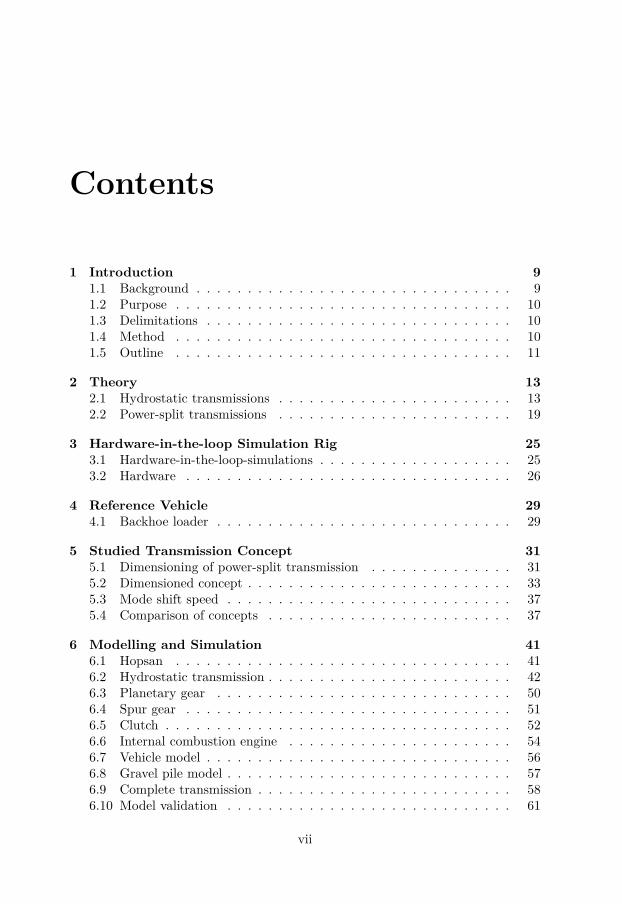
Contents
1 Introduction 91.1 Background . . . . . . . . . . . . . . . . . . . . . . . . . . . . . . . 91.2 Purpose . . . . . . . . . . . . . . . . . . . . . . . . . . . . . . . . . 101.3 Delimitations . . . . . . . . . . . . . . . . . . . . . . . . . . . . . . 101.4 Method . . . . . . . . . . . . . . . . . . . . . . . . . . . . . . . . . 101.5 Outline . . . . . . . . . . . . . . . . . . . . . . . . . . . . . . . . . 11
2 Theory 132.1 Hydrostatic transmissions . . . . . . . . . . . . . . . . . . . . . . . 132.2 Power-split transmissions . . . . . . . . . . . . . . . . . . . . . . . 19
3 Hardware-in-the-loop Simulation Rig 253.1 Hardware-in-the-loop-simulations . . . . . . . . . . . . . . . . . . . 253.2 Hardware . . . . . . . . . . . . . . . . . . . . . . . . . . . . . . . . 26
4 Reference Vehicle 294.1 Backhoe loader . . . . . . . . . . . . . . . . . . . . . . . . . . . . . 29
5 Studied Transmission Concept 315.1 Dimensioning of power-split transmission . . . . . . . . . . . . . . 315.2 Dimensioned concept . . . . . . . . . . . . . . . . . . . . . . . . . . 335.3 Mode shift speed . . . . . . . . . . . . . . . . . . . . . . . . . . . . 375.4 Comparison of concepts . . . . . . . . . . . . . . . . . . . . . . . . 37
6 Modelling and Simulation 416.1 Hopsan . . . . . . . . . . . . . . . . . . . . . . . . . . . . . . . . . 416.2 Hydrostatic transmission . . . . . . . . . . . . . . . . . . . . . . . . 426.3 Planetary gear . . . . . . . . . . . . . . . . . . . . . . . . . . . . . 506.4 Spur gear . . . . . . . . . . . . . . . . . . . . . . . . . . . . . . . . 516.5 Clutch . . . . . . . . . . . . . . . . . . . . . . . . . . . . . . . . . . 526.6 Internal combustion engine . . . . . . . . . . . . . . . . . . . . . . 546.7 Vehicle model . . . . . . . . . . . . . . . . . . . . . . . . . . . . . . 566.8 Gravel pile model . . . . . . . . . . . . . . . . . . . . . . . . . . . . 576.9 Complete transmission . . . . . . . . . . . . . . . . . . . . . . . . . 586.10 Model validation . . . . . . . . . . . . . . . . . . . . . . . . . . . . 61
vii
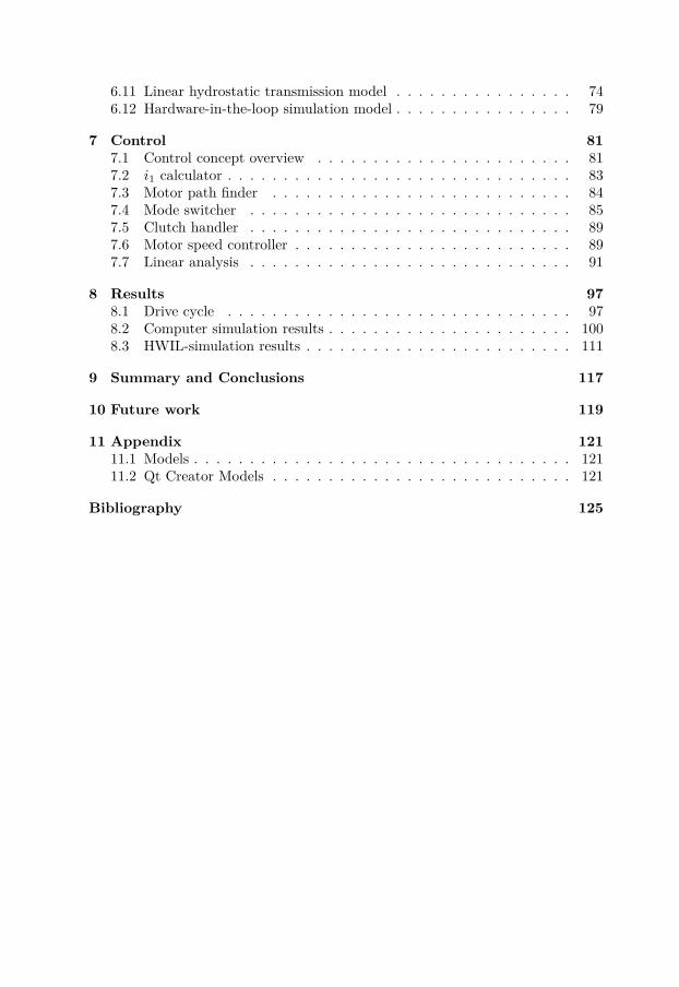
6.11 Linear hydrostatic transmission model . . . . . . . . . . . . . . . . 746.12 Hardware-in-the-loop simulation model . . . . . . . . . . . . . . . . 79
7 Control 817.1 Control concept overview . . . . . . . . . . . . . . . . . . . . . . . 817.2 i1 calculator . . . . . . . . . . . . . . . . . . . . . . . . . . . . . . . 837.3 Motor path finder . . . . . . . . . . . . . . . . . . . . . . . . . . . 847.4 Mode switcher . . . . . . . . . . . . . . . . . . . . . . . . . . . . . 857.5 Clutch handler . . . . . . . . . . . . . . . . . . . . . . . . . . . . . 897.6 Motor speed controller . . . . . . . . . . . . . . . . . . . . . . . . . 897.7 Linear analysis . . . . . . . . . . . . . . . . . . . . . . . . . . . . . 91
8 Results 978.1 Drive cycle . . . . . . . . . . . . . . . . . . . . . . . . . . . . . . . 978.2 Computer simulation results . . . . . . . . . . . . . . . . . . . . . . 1008.3 HWIL-simulation results . . . . . . . . . . . . . . . . . . . . . . . . 111
9 Summary and Conclusions 117
10 Future work 119
11 Appendix 12111.1 Models . . . . . . . . . . . . . . . . . . . . . . . . . . . . . . . . . . 12111.2 Qt Creator Models . . . . . . . . . . . . . . . . . . . . . . . . . . . 121
Bibliography 125
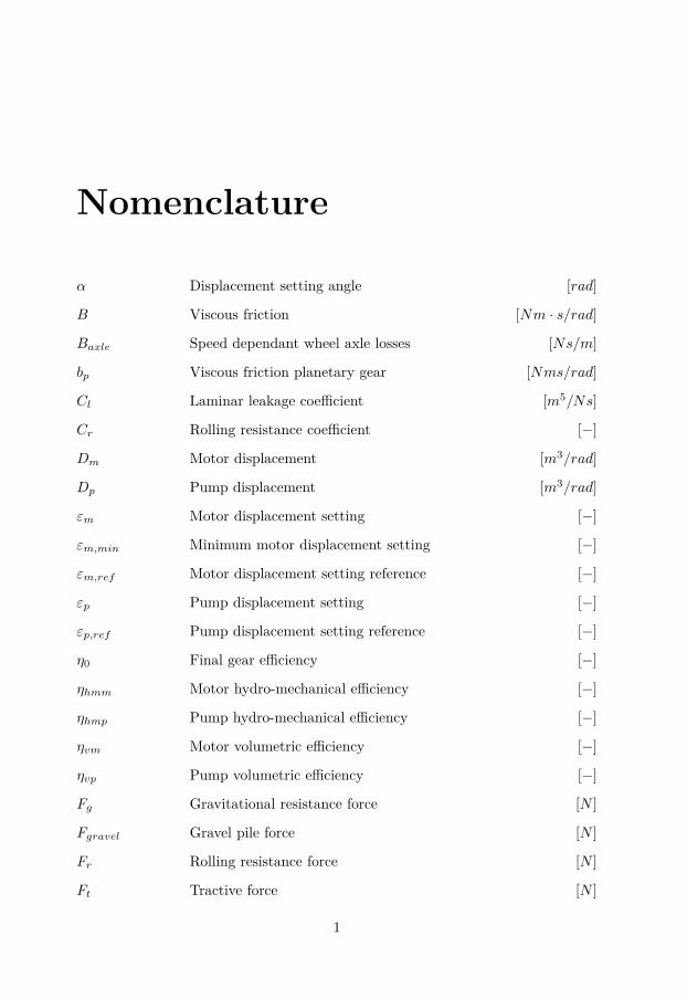
Nomenclature
α Displacement setting angle [rad]
B Viscous friction [Nm · s/rad]
Baxle Speed dependant wheel axle losses [Ns/m]
bp Viscous friction planetary gear [Nms/rad]
Cl Laminar leakage coefficient [m5/Ns]
Cr Rolling resistance coefficient [−]
Dm Motor displacement [m3/rad]
Dp Pump displacement [m3/rad]
εm Motor displacement setting [−]
εm,min Minimum motor displacement setting [−]
εm,ref Motor displacement setting reference [−]
εp Pump displacement setting [−]
εp,ref Pump displacement setting reference [−]
η0 Final gear efficiency [−]
ηhmm Motor hydro-mechanical efficiency [−]
ηhmp Pump hydro-mechanical efficiency [−]
ηvm Motor volumetric efficiency [−]
ηvp Pump volumetric efficiency [−]
Fg Gravitational resistance force [N ]
Fgravel Gravel pile force [N ]
Fr Rolling resistance force [N ]
Ft Tractive force [N ]
1
2 Contents
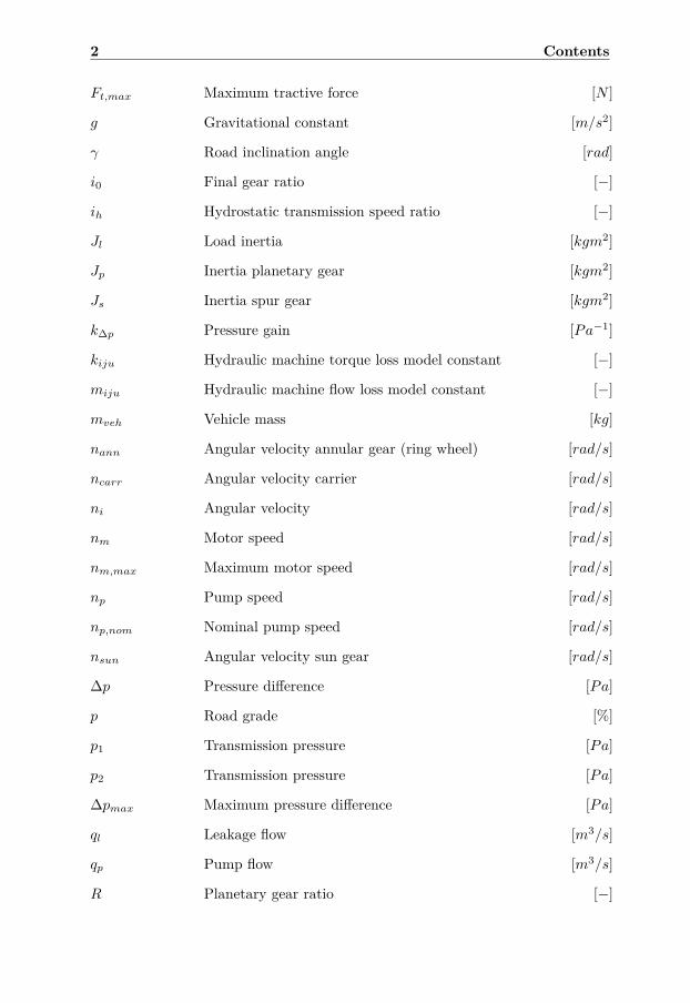
Ft,max Maximum tractive force [N ]
g Gravitational constant [m/s2]
γ Road inclination angle [rad]
i0 Final gear ratio [−]
ih Hydrostatic transmission speed ratio [−]
Jl Load inertia [kgm2]
Jp Inertia planetary gear [kgm2]
Js Inertia spur gear [kgm2]
k∆p Pressure gain [Pa−1]
kiju Hydraulic machine torque loss model constant [−]
miju Hydraulic machine flow loss model constant [−]
mveh Vehicle mass [kg]
nann Angular velocity annular gear (ring wheel) [rad/s]
ncarr Angular velocity carrier [rad/s]
ni Angular velocity [rad/s]
nm Motor speed [rad/s]
nm,max Maximum motor speed [rad/s]
np Pump speed [rad/s]
np,nom Nominal pump speed [rad/s]
nsun Angular velocity sun gear [rad/s]
∆p Pressure difference [Pa]
p Road grade [%]
p1 Transmission pressure [Pa]
p2 Transmission pressure [Pa]
∆pmax Maximum pressure difference [Pa]
ql Leakage flow [m3/s]
qp Pump flow [m3/s]
R Planetary gear ratio [−]
Contents 3
rw Wheel radius [m]
T0 Transmission output torque [Nm]
Tann Torque annular gear (ring wheel) [Nm]
Tcarr Torque carrier [Nm]
Ti Torque [Nm]
TICE Internal combustion engine input torque [Nm]
Tl Torque losses [Nm]
Tm Motor torque [Nm]
Tm,max Maximum motor torque [Nm]
Tp Pump torque [Nm]
Tsun Torque sun gear [Nm]
Vbucket Front loader bucket size [m3]
Vs System volume [m3]
vveh Vehicle velocity [m/s]
vveh,max Maximum vehicle velocity [m/s]
ω∆p Pressure filter break frequency [rad/s]
ωm Motor displacement controller break frequency [rad/s]
ωp− Pump displacement controller break frequency, negative displace-ment [rad/s]
ωp+ Pump displacement controller break frequency, positive displace-ment [rad/s]
xveh Vehicle travelled distance [m]
yh,p/m Pump/motor displacement controller hysteresis width [−]
4 Contents
List of Figures2.1 Ideal hydrostatic transmission. . . . . . . . . . . . . . . . . . . . . 132.2 CVT and IVT behaviour. . . . . . . . . . . . . . . . . . . . . . . . 142.3 Ideal hydrostatic transmission with auxiliary components. . . . . . 152.4 In-line (left) and bent-axis (right) axial piston machine working
principals. . . . . . . . . . . . . . . . . . . . . . . . . . . . . . . . . 152.5 In-line (left) and bent-axis (right) machine displacement controllers. 162.6 Vehicle speed versus tractive force requirement for maximum con-
stant input power. . . . . . . . . . . . . . . . . . . . . . . . . . . . 172.7 Principle sketch of PST concept with a mechanical drive train par-
allel to a variator. The arrows symbolise the power flow. . . . . . . 192.8 Planetary gear set with its components. Annular gear (green),
planet gear (black), sun gear (red) and the carrier (blue). . . . . . 202.9 a) ICPS and b) OCPS with input shaft to the left and output shaft
to the right. . . . . . . . . . . . . . . . . . . . . . . . . . . . . . . . 212.10 Power flow through an ICPS (figure 2.9 a)) for the different modes.
Input power to the left and output power to the right. . . . . . . . 222.11 Lever diagram of ICPS which describes when the different kinds of
power flow modes occur. . . . . . . . . . . . . . . . . . . . . . . . . 232.12 Jarchow’s two modes power-split transmission. . . . . . . . . . . . 23
3.1 Hardware-in-the-loop-simulation rig schematics. . . . . . . . . . . . 263.2 Machine and servo valve on the drive side. . . . . . . . . . . . . . . 263.3 Rig communication visualisation. . . . . . . . . . . . . . . . . . . . 273.4 Pump (left) and motor (right) in the hydrostatic transmission circuit. 283.5 Accumulators used in the hydrostatic transmission circuit. . . . . . 28
4.1 Volvo backhoe loader. . . . . . . . . . . . . . . . . . . . . . . . . . 294.2 Volvo backhoe loader in action. . . . . . . . . . . . . . . . . . . . . 30
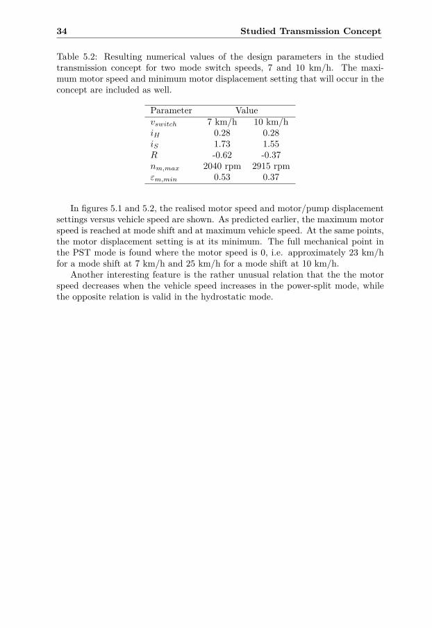
5.1 Motor speed and motor/pump displacement settings versus vehiclespeed when mode shift occurs at 7 km/h (i.e. power-split mode isentered at |vveh| > 7 km/h). . . . . . . . . . . . . . . . . . . . . . . 35
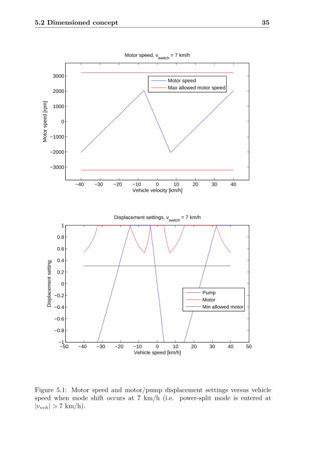
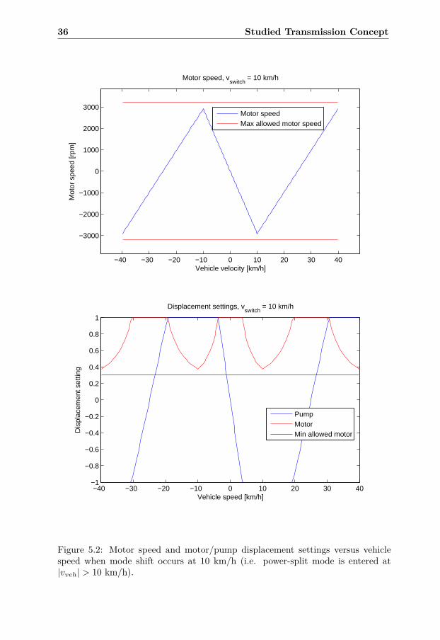
5.2 Motor speed and motor/pump displacement settings versus vehiclespeed when mode shift occurs at 10 km/h (i.e. power-split mode isentered at |vveh| > 10 km/h). . . . . . . . . . . . . . . . . . . . . . 36
5.3 Force-velocity graph for torque converter with 64 kW engine andpower-split with 55 kW engine. . . . . . . . . . . . . . . . . . . . . 38
6.1 Boost circuit and cooling circuit as they are modelled in Hopsan. . 426.2 Pump actuator as modelled in Hopsan. . . . . . . . . . . . . . . . . 436.3 Motor actuator as modelled in Hopsan. . . . . . . . . . . . . . . . 446.4 Transmission pump with efficiency model as modelled in Hopsan. . 446.5 Transmission motor with efficiency model as modelled in Hopsan. . 45
Contents 5
6.6 Flow and torque losses for the pump calculated from the loss modelfor different pressure differences and speeds. The displacement set-ting is εp = 1. . . . . . . . . . . . . . . . . . . . . . . . . . . . . . . 47
6.7 Flow and torque losses for the motor calculated from the loss modelfor different pressure differences and speeds. The displacement set-ting is εm = 1.0. . . . . . . . . . . . . . . . . . . . . . . . . . . . . 47
6.8 Volumetric and hydro-mechanical efficiencies for the pump calcu-lated from the loss model for different pressure differences andspeeds. The displacement setting is εp = 1. . . . . . . . . . . . . . 48
6.9 Total efficiency for the motor calculated from the loss model fordifferent pressure differences and speeds. The displacement settingis εm = 0.3 in the left graph and εm = 1 in the right graph. . . . . 49
6.10 Total efficiency for the pump calculated from the loss model fordifferent pressure differences and speeds. The displacement settingis εp = 0.3 in the left graph and εp = 1 in the right graph. . . . . . 50
6.11 Planetary gear model. . . . . . . . . . . . . . . . . . . . . . . . . . 506.12 Free body diagram of planetary gear model. . . . . . . . . . . . . . 516.13 Spur gear models. . . . . . . . . . . . . . . . . . . . . . . . . . . . 516.14 Wet disc clutch working principal. . . . . . . . . . . . . . . . . . . 526.15 Small example system with a clutch in Hopsan. . . . . . . . . . . . 536.16 Results from the example clutch system. The clutch is engaged
during at 1 second. A step disturbance torque of 200 Nm is addedat 3 seconds. . . . . . . . . . . . . . . . . . . . . . . . . . . . . . . 54
6.17 Schematics of the combustion engine model. . . . . . . . . . . . . . 546.18 Torque-velocity curve for the used combustion engine model. . . . 556.19 Gravel pile resisting force as calculated by the gravel pile model for
0-3 m into a pile. . . . . . . . . . . . . . . . . . . . . . . . . . . . . 586.20 Complete vehicle- and transmission model as implemented in Hopsan. 606.21 Pump displacement controller validation model as implemented in
Hopsan. . . . . . . . . . . . . . . . . . . . . . . . . . . . . . . . . . 626.22 Validation of pump displacement controller, during low load. . . . 636.23 Validation of pump displacement controller during high load. . . . 636.24 Transmission validation model as implemented in Hopsan. . . . . . 656.25 Input signals to the transmission validation model, test 1. . . . . . 666.26 Output signals from the transmission validation model and corre-
sponding measured data from the rig, test 1. . . . . . . . . . . . . 676.27 Input signals to the transmission validation model, test 2. . . . . . 686.28 Output signals from the transmission validation model and corre-
sponding measured data from the rig, test 2. . . . . . . . . . . . . 696.29 Input signals to the transmission validation model, test 3. . . . . . 706.30 Output signals from the transmission validation model and corre-
sponding measured data from the rig, test 3. . . . . . . . . . . . . 716.31 Input signals to the transmission validation model, test 4. . . . . . 726.32 Output signals from the transmission validation model and corre-
sponding measured data from the rig, test 4. . . . . . . . . . . . . 73
6 Contents
6.33 Open loop system linearised around displacement setting εm,0 = 1.Hydrostatic mode left and power-split mode right. . . . . . . . . . 76
6.34 Differences in system characteristics depending on the current mode(hydrostatic or power-split). . . . . . . . . . . . . . . . . . . . . . . 77
6.35 Bode diagram for hydrostatic mode with different displacement set-tings of the motor displacement. . . . . . . . . . . . . . . . . . . . 78
6.36 Bode diagram for power-split mode with different displacement set-tings of the motor displacement. . . . . . . . . . . . . . . . . . . . 78
6.37 Layout for the Simulink transmission model used in the Hardware-in-the-loop simulations. . . . . . . . . . . . . . . . . . . . . . . . . 79
7.1 Simplified version of the studied transmission concept. . . . . . . . 817.2 Jarchow transmission concept studied in the project. . . . . . . . . 827.3 Layout of the complete transmission controller implemented in simulink. 837.4 i1 calculator sub controller in the transmission controller as imple-
mented in Simulink. . . . . . . . . . . . . . . . . . . . . . . . . . . 847.5 Motor path finder sub controller in the transmission controller as
implemented in Simulink. . . . . . . . . . . . . . . . . . . . . . . . 847.6 Visualised relay effect used in the mode switcher sub controller. . . 857.7 Visualised window effect used in the mode switcher sub controller
to decide whether a clutch is synchronised. . . . . . . . . . . . . . 867.8 Decision tree corresponding to the logic used in the mode switcher
sub controller to know when to switch between power-split modeand hydrostatic mode. The red paths describes the controllers de-cisions the time step before a mode shift and the time step after amode shift, when the mode switches from hydrostatic to power-split. 87
7.9 Mode switcher sub controller in the transmission controller as im-plemented in Simulink. . . . . . . . . . . . . . . . . . . . . . . . . . 88
7.10 ”Clutch handler” sub controller as implemented in Simulink. . . . 897.11 Block diagram of transmission system with PI-control Freg, feed-
forward control Ffr and transfer function Gsys from reference signalto output signal. . . . . . . . . . . . . . . . . . . . . . . . . . . . . 90
7.12 Bode diagram with stability margins for the derived linear model,including the controller PI, from displacement setting to angularvelocity. The system is linearised in εm,0 = 1. Hydrostatic mode tothe left and power-split mode to the right. . . . . . . . . . . . . . . 92
7.13 Bode diagram with stability margins for the derived linear model,including the controller PI, from displacement setting to angularvelocity. The system is linearised in εm,0 = 0.3. Hydrostatic modeto the left and power-split mode to the right.. . . . . . . . . . . . . 93
8.1 Sketch of load-carry drive cycle. . . . . . . . . . . . . . . . . . . . . 988.2 Velocity of vehicle in load-carry drive cycle. . . . . . . . . . . . . . 988.3 Sketch of ramp digging drive cycle. . . . . . . . . . . . . . . . . . . 998.4 Velocity of vehicle in ramp digging drive cycle. . . . . . . . . . . . 998.5 Vehicle speed. . . . . . . . . . . . . . . . . . . . . . . . . . . . . . . 100
Contents 7
8.6 Motor speed. . . . . . . . . . . . . . . . . . . . . . . . . . . . . . . 1018.7 Motor torque. . . . . . . . . . . . . . . . . . . . . . . . . . . . . . . 1028.8 Transmission output torque. . . . . . . . . . . . . . . . . . . . . . . 1038.9 Transmission pressure. . . . . . . . . . . . . . . . . . . . . . . . . . 1038.10 Pump/ICE speed. . . . . . . . . . . . . . . . . . . . . . . . . . . . 1048.11 Internal combustion engine torque. . . . . . . . . . . . . . . . . . . 1058.12 Transmission machine displacement settings. . . . . . . . . . . . . 1068.13 Transmission controller signals. . . . . . . . . . . . . . . . . . . . . 1068.14 Vehicle speed. . . . . . . . . . . . . . . . . . . . . . . . . . . . . . . 1078.15 Motor speed at mode shift from hydrostatic to power-split. . . . . 1088.16 Transmission output torque at mode shift from hydrostatic to power-
split. The signals to the involved clutches SH and SF W D are in-cluded as well. The clutch signals vary between 0 and 1 but arehere scaled to fit in the graph. . . . . . . . . . . . . . . . . . . . . . 108
8.17 Vehicle speed step response in hydrostatic mode with the displace-ment setting of the machine (pump or motor) currently handlingthe control, as sent by the controller. . . . . . . . . . . . . . . . . . 110
8.18 Vehicle speed step response in power-split mode. . . . . . . . . . . 1108.19 Motor speed. . . . . . . . . . . . . . . . . . . . . . . . . . . . . . . 1128.20 Vehicle speed. . . . . . . . . . . . . . . . . . . . . . . . . . . . . . . 1138.21 Motor torques. ”Rig torque” is referring to the torque that is sent
and controlled by the load side controller in the rig, after it hasbeen compensated for the rig inertia. ”Motor torque” refers to theactual torque that the motor experiences (i.e. the torque that themotor would experience in a real vehicle). . . . . . . . . . . . . . . 113
8.22 Pump/engine speed. . . . . . . . . . . . . . . . . . . . . . . . . . . 1148.23 Pump torque. . . . . . . . . . . . . . . . . . . . . . . . . . . . . . . 1158.24 Transmission pressures. . . . . . . . . . . . . . . . . . . . . . . . . 1158.25 Transmission machine displacement settings. . . . . . . . . . . . . 1168.26 Transmission controller signals. . . . . . . . . . . . . . . . . . . . . 116
8 Contents
List of Tables4.1 Backhoe specifications. . . . . . . . . . . . . . . . . . . . . . . . . . 30
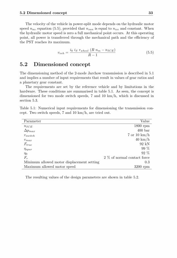
5.1 Numerical input requirements for dimensioning the transmissionconcept. Two switch speeds, 7 and 10 km/h, are tried out. . . . . . 33
5.2 Resulting numerical values of the design parameters in the studiedtransmission concept for two mode switch speeds, 7 and 10 km/h.The maximum motor speed and minimum motor displacement set-ting that will occur in the concept are included as well. . . . . . . 34
5.3 Requirement of backhoe application. . . . . . . . . . . . . . . . . . 37
6.1 Pump loss model constants. . . . . . . . . . . . . . . . . . . . . . . 466.2 Motor loss model constants. . . . . . . . . . . . . . . . . . . . . . . 466.3 Values used for the parameters in the combustion engine model. . 566.4 Values used for the parameters in the vehicle mechanical model. . 576.5 Values used for the parameters in the gravel pile model. . . . . . . 586.6 Values used for the parameters in the pump displacement controller
validation model. . . . . . . . . . . . . . . . . . . . . . . . . . . . . 626.7 Values used for the parameters in the hydrostatic transmission val-
idation model. . . . . . . . . . . . . . . . . . . . . . . . . . . . . . . 646.8 Values used for the parameters in the linear model of the hydrostatic
transmission. The values for the inertia are displayed in table 6.9. 756.9 Equivalent motor inertias for studied transmission concept at a
mode shift speed of 7 km/h . . . . . . . . . . . . . . . . . . . . . . 75
7.1 Parameter values for PI-controller gains and the feed forward gainused both in the computer simulations and the HWIL-simulations. 91
Chapter 1
Introduction
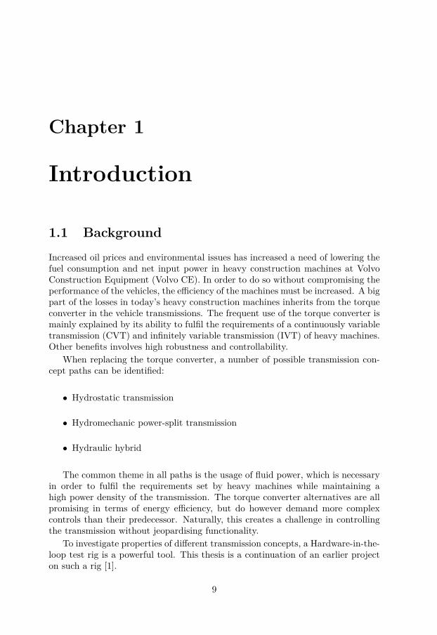
1.1 Background
Increased oil prices and environmental issues has increased a need of lowering thefuel consumption and net input power in heavy construction machines at VolvoConstruction Equipment (Volvo CE). In order to do so without compromising theperformance of the vehicles, the efficiency of the machines must be increased. A bigpart of the losses in today’s heavy construction machines inherits from the torqueconverter in the vehicle transmissions. The frequent use of the torque converter ismainly explained by its ability to fulfil the requirements of a continuously variabletransmission (CVT) and infinitely variable transmission (IVT) of heavy machines.Other benefits involves high robustness and controllability.
When replacing the torque converter, a number of possible transmission con-cept paths can be identified:
• Hydrostatic transmission
• Hydromechanic power-split transmission
• Hydraulic hybrid
The common theme in all paths is the usage of fluid power, which is necessaryin order to fulfil the requirements set by heavy machines while maintaining ahigh power density of the transmission. The torque converter alternatives are allpromising in terms of energy efficiency, but do however demand more complexcontrols than their predecessor. Naturally, this creates a challenge in controllingthe transmission without jeopardising functionality.
To investigate properties of different transmission concepts, a Hardware-in-the-loop test rig is a powerful tool. This thesis is a continuation of an earlier projecton such a rig [1].
9
10 Introduction
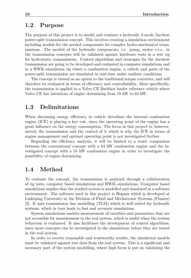
1.2 PurposeThe purpose of this project is to model and evaluate a hydraulic 2-mode Jarchowpower-split transmission concept. This involves creating a simulation environmentincluding models for the needed components for complex hydro-mechanical trans-missions. The models of the hydraulic components, i.e. pump, motor e.t.c., inthe transmission concepts will be validated against hardware tests in a test rigfor hydrostatic transmissions. Control algorithms and strategies for the Jarchowtransmission are going to be developed and evaluated in computer simulations andin a HWIL-simulation rig where a combustion engine, a vehicle and parts of thepower-split transmission are simulated in real-time under realistic conditions.
The concept is viewed as an option to the traditional torque converter, and willtherefore be evaluated in terms of efficiency and controllability. More specifically,the transmission is applied to a Volvo CE Backhoe loader reference vehicle whereVolvo CE has intentions of engine downsizing from 55 kW to 64 kW.
1.3 DelimitationsWhen discussing energy efficiency in vehicle drivelines the internal combustionengine (ICE) is playing a key role, since the operating point of the engine has agreat influence on the energy consumption. The focus in this project is, however,merely the transmission and the control of it which is why the ICE in terms ofengine management and optimal operating point is not investigated further.
Regarding the efficiency analysis, it will be limited to a static comparisonbetween the conventional concept with a 64 kW combustion engine and the in-vestigated concept with a 55 kW combustion engine in order to investigate thepossibility of engine downsizing.
1.4 MethodTo evaluate the concept, the transmission is analysed through a collaborationof rig tests, computer based simulations and HWIL-simulations. Computer basedsimulations implies that the studied system is modelled and simulated in a softwareenvironment. The software used in this project is Hopsan which is developed atLinköping University at the Division of Fluid and Mechatronic Systems (Flumes)[2]. It uses transmission line modelling (TLM) which is well suited for hydraulicsystems, which in turn leads to fast and accurate simulations.
System simulations enables measurement of variables and parameters that arenot accessible for measurement in the real system, which is useful when the systembehaviour is evaluated. It also facilitates the development of control algorithms,since more concepts can be investigated in the simulations before they are testedin the real system.
In order to receive reasonable and trustworthy results, the simulation modelsmust be validated against test data from the real system. This is a significant andnecessary part of the system modelling, where high focus is put on validating the
1.5 Outline 11
losses in the system. The system tests are carried out in a test rig including ahydrostatic transmission.
The control algorithms are developed in Matlab/Simulink, and tested in theHopsan simulation models before they are tested in the system.
When the transmission is modelled it is implemented in a HWIL-simulationrig, where the reference vehicle is simulated under realistic conditions to evaluatethe transmission performance. A great benefit with the HWIL-simulation rig is thepossibility to actually include one of the most complex parts of the transmission,i.e. the hydrostatic transmission, as hardware and model everything around it.Thereby, the results are more trustworthy and applicable on a realistic situation.
1.5 OutlineThe second, third and fourth chapters in this thesis are making up the basisand the frame in which the preferences of the complete thesis are captured. Thesecond chapter concerns the theory of the studied concept, where the behaviourof the hydrostatic transmission, the power-split transmission and the componentswithin are elucidated. The third chapter continues by explaining the concept ofHardware-in-the-loop simulations and describing the HWIL simulation rig used inthis project. The fourth chapter describes the Backhoe loader reference vehiclefor which the transmission concept will be evaluated. This includes the machineapplication area, vehicle specifications and a description of the currently usedtransmission.
The fifth chapter contains a more specific description of the studied power-splittransmission concept, and how it is dimensioned in order to fit the reference vehiclewithin the frames previously set, such as HWIL-simulation rig limitations. A com-parison between the power-split transmission concept a conventional transmissionconcept is carried out as well.
The sixth chapter is devoted to all the modelling carried out in the thesis.Hopsan itself and the models derived in Hopsan in order to simulate the trans-mission are displayed and described. The validation work regarding the hydraulicmodels (pump, motor etc.) is also found here. Furthermore, a linear model ofthe transmission and the model used for the HWIL-simulations are derived in thischapter.
In the seventh chapter the basics of the transmission control strategy used inthis thesis are explained and described. The Simulink controller with sub con-trollers are explained, and the linear model derived in the sixth chapter is used toanalyse the implemented controller.
The eighth chapter displays and discusses the computer simulation and theHWIL simulation results. The drive cycles used in order to evaluate the transmis-sion are described as well.
In the ninth chapter the work is summarised and important conclusions aredrawn. The tenth chapter contains information regarding future work that maybe viewed as a proper continuation of this project. Finally, the eleventh chapterconsists of the appendix where the C-code for the clutch model is inserted.

12 Introduction
Chapter 2
Theory
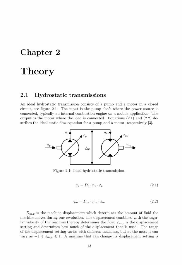
2.1 Hydrostatic transmissionsAn ideal hydrostatic transmission consists of a pump and a motor in a closedcircuit, see figure 2.1. The input is the pump shaft where the power source isconnected, typically an internal combustion engine on a mobile application. Theoutput is the motor where the load is connected. Equations (2.1) and (2.2) de-scribes the ideal static flow equation for a pump and a motor, respectively [3].
np nm
qp qmεp εm
∆p
Figure 2.1: Ideal hydrostatic transmission.
qp = Dp · np · εp (2.1)
qm = Dm · nm · εm (2.2)
Dm,p is the machine displacement which determines the amount of fluid themachine moves during one revolution. The displacement combined with the angu-lar velocity of the machine thereby determines the flow. εm,p is the displacementsetting and determines how much of the displacement that is used. The rangeof the displacement setting varies with different machines, but at the most it canvary as −1 6 εm,p 6 1. A machine that can change its displacement setting is
13
14 Theory
commonly referred to as a variable machine, whereas a machine that cannot doso is referred to as a fixed machine. There are exceptions, but in general thedisplacement setting varies continuously.
Ideally, i.e. if leakage is neglected, the pump flow is equal to the motor flow:
qm = qp (2.3)
(2.3) with (2.2) and (2.1) then yields the transmission speed ratio:
ih = nm
np= Dp · εp
Dm · εm∝ εp
εm(2.4)
(2.4) shows that the speed ratio of the transmission is determined by the dis-placement settings on the hydraulic machines used in the circuit. Normally, aconstant speed is assumed on the pump shaft. If the pump then can realise dis-placement settings as −1 6 εp 6 1, the output speed is controlled by changing εp,and negative speed is achieved by realising εp < 0. By having a variable motor aswell, the range of the speed ratio increases further.
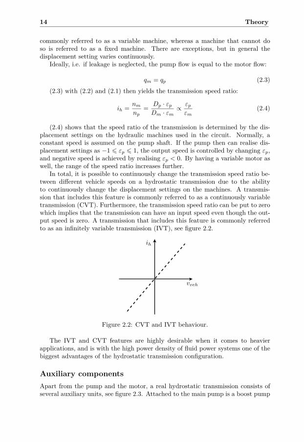
In total, it is possible to continuously change the transmission speed ratio be-tween different vehicle speeds on a hydrostatic transmission due to the abilityto continuously change the displacement settings on the machines. A transmis-sion that includes this feature is commonly referred to as a continuously variabletransmission (CVT). Furthermore, the transmission speed ratio can be put to zerowhich implies that the transmission can have an input speed even though the out-put speed is zero. A transmission that includes this feature is commonly referredto as an infinitely variable transmission (IVT), see figure 2.2.
vveh
ih
Figure 2.2: CVT and IVT behaviour.
The IVT and CVT features are highly desirable when it comes to heavierapplications, and is with the high power density of fluid power systems one of thebiggest advantages of the hydrostatic transmission configuration.
Auxiliary componentsApart from the pump and the motor, a real hydrostatic transmission consists ofseveral auxiliary units, see figure 2.3. Attached to the main pump is a boost pump
2.1 Hydrostatic transmissions 15
that cooperates with a pressure relief valve in order to maintain the pressure on thelow pressure-side to avoid cavitation. Check valves are needed since the low/highpressure sides alternates with the sign of the load. Two pressure relief valves areincluded as well, to avoid breakdown if the high pressure reaches too high levels.
The second circuit is the cooling circuit that continuously drains the lowpressure-side from oil.
Figure 2.3: Ideal hydrostatic transmission with auxiliary components.
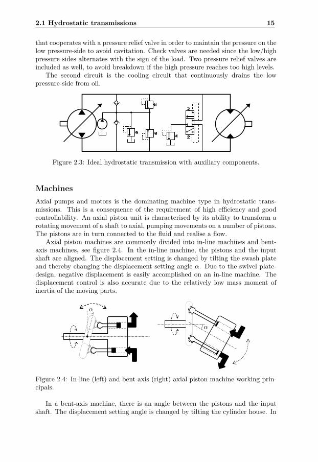
MachinesAxial pumps and motors is the dominating machine type in hydrostatic trans-missions. This is a consequence of the requirement of high efficiency and goodcontrollability. An axial piston unit is characterised by its ability to transform arotating movement of a shaft to axial, pumping movements on a number of pistons.The pistons are in turn connected to the fluid and realise a flow.
Axial piston machines are commonly divided into in-line machines and bent-axis machines, see figure 2.4. In the in-line machine, the pistons and the inputshaft are aligned. The displacement setting is changed by tilting the swash plateand thereby changing the displacement setting angle α. Due to the swivel plate-design, negative displacement is easily accomplished on an in-line machine. Thedisplacement control is also accurate due to the relatively low mass moment ofinertia of the moving parts.
α
α
Figure 2.4: In-line (left) and bent-axis (right) axial piston machine working prin-cipals.
In a bent-axis machine, there is an angle between the pistons and the inputshaft. The displacement setting angle is changed by tilting the cylinder house. In
16 Theory
a bent-axis machine, negative displacement settings are more difficult to achievesince the whole cylinder house would have to move a long distance, making themachine very bulky.
In general, the pump in a hydrostatic transmission is of an in-line design whilethe motor is of a bent-axis design. By having an in-line pump, negative velocity isachieved smoothly by moving into negative displacement. The benefits of a bent-axis motor is mainly that the bent-axis machine has a better efficiency duringlower speeds than the in-line machine, which is important for the motor since themotor speed is directly coupled to the vehicle speed.
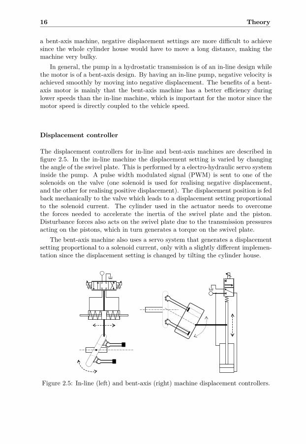
Displacement controller
The displacement controllers for in-line and bent-axis machines are described infigure 2.5. In the in-line machine the displacement setting is varied by changingthe angle of the swivel plate. This is performed by a electro-hydraulic servo systeminside the pump. A pulse width modulated signal (PWM) is sent to one of thesolenoids on the valve (one solenoid is used for realising negative displacement,and the other for realising positive displacement). The displacement position is fedback mechanically to the valve which leads to a displacement setting proportionalto the solenoid current. The cylinder used in the actuator needs to overcomethe forces needed to accelerate the inertia of the swivel plate and the piston.Disturbance forces also acts on the swivel plate due to the transmission pressuresacting on the pistons, which in turn generates a torque on the swivel plate.
The bent-axis machine also uses a servo system that generates a displacementsetting proportional to a solenoid current, only with a slightly different implemen-tation since the displacement setting is changed by tilting the cylinder house.
Figure 2.5: In-line (left) and bent-axis (right) machine displacement controllers.
2.1 Hydrostatic transmissions 17
LossesIn comparison to a purely mechanical transmission, the hydrostatic transmissionsuffers from a rather poor efficiency. The losses inside the machines can be dividedin two types generally referred to as hydro-mechanical losses and volumetric losses.
The hydro-mechanical losses represents all the torque and pressure losses in amachine. The main contribution to this part comes from dry and viscous frictionin all moving parts in the machines. There are also torque losses due to theacceleration of the moving parts (pistons, cylinder drum e.t.c.). When the machinespeed becomes very high, the torque losses increases significantly due to the highvelocity of the parts moving in oil, a phenomenon commonly referred to as ”splash”losses.
The volumetric losses represent all the losses in flow and speed in the machines.The main part of these losses is leakage from the high pressure-side to either thelow pressure-side in the transmission or to tank. Additional flow losses occurswhen the oil is compressed.
Apart from the internal losses in the machines, the auxiliary units also con-tributes. The main part here inherits from the boost pump. The boost pumpis connected to the same shaft as the main pump, and works under a constantpressure. The boost pump loss is thereby mainly a torque loss proportional to thepressure in the boost circuit.
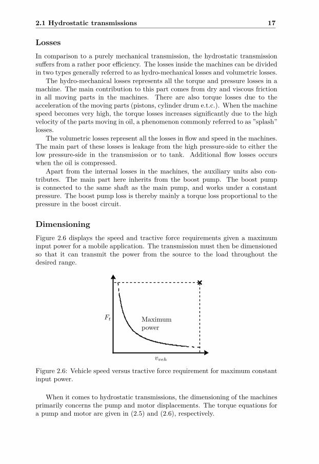
DimensioningFigure 2.6 displays the speed and tractive force requirements given a maximuminput power for a mobile application. The transmission must then be dimensionedso that it can transmit the power from the source to the load throughout thedesired range.
vveh
Ft Maximumpower
Figure 2.6: Vehicle speed versus tractive force requirement for maximum constantinput power.
When it comes to hydrostatic transmissions, the dimensioning of the machinesprimarily concerns the pump and motor displacements. The torque equations fora pump and motor are given in (2.5) and (2.6), respectively.
18 Theory
Tp = ∆p ·Dp · εp (2.5)
Tm = ∆p ·Dm · εm (2.6)
The requirement of maximum tractive force can be translated into a maximumtorque Tm on the motor. Given that maximum torque is reached at εm = 1and a maximum allowed system pressure, the motor displacement is determinedaccording to (2.7).
Dm = Tm,max
∆pmax(2.7)
The pump displacement is determined by the requirement of maximum vehiclespeed that in turn implies a requirement of maximum flow. Maximum vehiclespeed can be translated to a maximum motor speed which is reached at εp = 1and εm = εm,min. If the pump speed then is determined by the nominal speed ofthe power source, the pump displacement is determined from (2.4) according to(2.8).
Dp = Dm · nm,max · εm,min
np,nom(2.8)
As seen in (2.7) and (2.8), the machine displacements are directly determinedby the extreme conditions regarding vehicle speed and tractive force. Another wayof expressing this is to state that the hydrostatic transmission is dimensioned forthe corner power, i.e. Ft,max ·vveh,max, see figure 2.6. By adding a gearbox betweenthe motor and the load, this effect can be lowered. The gearbox must howeverbe of the power-shift type, since the gear shifting must take place without losingtractive force. In lighter applications, such as smaller wheel loaders, a hydrostatictransmission with a power-shift gearbox is a commonly used concept [4].
Heavier applicationsHeavier applications imply an increased required maximum tractive force. Sincethe limit in system pressure is set by other factors1 than vehicle size, equation(2.7) yields that a heavy application will suffer from a highly oversized motor.There are several examples of how this problem can be addressed, see for example[4] and [5].
Another issue in larger applications is that the relatively2 low efficiency of thehydrostatic transmission leads to unreasonably high losses when the power flowincreases.
1Typically the highest allowed pressure in a circuit is around 300 - 400 bar, where too highpressures causes either damage to equipment or unacceptably high leakages.
2Mainly compared to a purely mechanical transmission
2.2 Power-split transmissions 19
A conventional hydrostatic transmission is mainly controlled by changing thepump displacement setting. Given equation (2.1), this means that the control sig-nal corresponds to a flow and a speed on the output shaft. In a heavier application,the requirement of traction control, i.e. controlling the tractive force, is stricterdue to the increased load, which thus argues against the use of pure hydrostaticdrive in a heavy application.
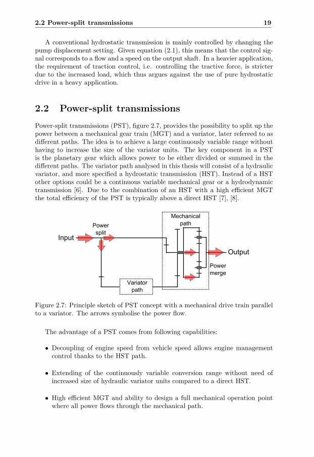
2.2 Power-split transmissionsPower-split transmissions (PST), figure 2.7, provides the possibility to split up thepower between a mechanical gear train (MGT) and a variator, later refereed to asdifferent paths. The idea is to achieve a large continuously variable range withouthaving to increase the size of the variator units. The key component in a PSTis the planetary gear which allows power to be either divided or summed in thedifferent paths. The variator path analysed in this thesis will consist of a hydraulicvariator, and more specified a hydrostatic transmission (HST). Instead of a HSTother options could be a continuous variable mechanical gear or a hydrodynamictransmission [6]. Due to the combination of an HST with a high efficient MGTthe total efficiency of the PST is typically above a direct HST [7], [8].
MechanicalpathPower
split
Powermerge
Variatorpath
Input
Output
Figure 2.7: Principle sketch of PST concept with a mechanical drive train parallelto a variator. The arrows symbolise the power flow.
The advantage of a PST comes from following capabilities:
• Decoupling of engine speed from vehicle speed allows engine managementcontrol thanks to the HST path.
• Extending of the continuously variable conversion range without need ofincreased size of hydraulic variator units compared to a direct HST.
• High efficient MGT and ability to design a full mechanical operation pointwhere all power flows through the mechanical path.
20 Theory
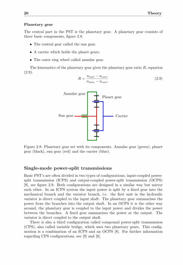
Planetary gear
The central part in the PST is the planetary gear. A planetary gear consists ofthree basic components, figure 2.8.
• The central gear called the sun gear.
• A carrier which holds the planet gears.
• The outer ring wheel called annular gear.
The kinematics of the planetary gear gives the planetary gear ratio R, equation(2.9).
R = nsun − ncarr
nann − ncarr(2.9)
Annular gearPlanet gear
Sun gear Carrier
Figure 2.8: Planetary gear set with its components. Annular gear (green), planetgear (black), sun gear (red) and the carrier (blue).
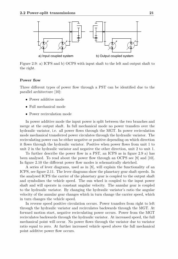
Single-mode power-split transmissionsBasic PST’s are often divided in two types of configurations, input-coupled power-split transmission (ICPS) and output-coupled power-split transmission (OCPS)[9], see figure 2.9. Both configurations are designed in a similar way but mirroreach other. In an ICPS system the input power is split by a fixed gear into themechanical branch and the variator branch, i.e. the first unit in the hydraulicvariator is direct coupled to the input shaft. The planetary gear summarises thepower from the branches into the output shaft. In an OCPS it is the other wayaround, the planetary gear is coupled to the input power and divides the powerbetween the branches. A fixed gear summarises the power at the output. Thevariator is direct coupled to the output shaft.
There is also a third configuration called compound power-split transmission(CPS), also called variable bridge, which uses two planetary gears. This config-uration is a combination of an ICPS and an OCPS [8]. For further informationregarding CPS configurations, see [8] and [6].
2.2 Power-split transmissions 21
a) Input coupled system b) Output coupled system
Figure 2.9: a) ICPS and b) OCPS with input shaft to the left and output shaft tothe right.
Power flow
Three different types of power flow through a PST can be identified due to theparallel architecture [10]:
• Power additive mode
• Full mechanical mode
• Power recirculation mode
In power additive mode the input power is split between the two branches andmerge at the output shaft. In full mechanical mode no power transfers over thehydraulic variator, i.e. all power flows through the MGT. In power recirculationmode mechanical transferred power circulates through the hydraulic variator. Therecirculating power can be either negative or positive depending on which directionit flows through the hydraulic variator. Positive when power flows from unit 1 tounit 2 in the hydraulic variator and negative the other direction, unit 2 to unit 1.
To further describe the power flow in a PST, an ICPS as in figure 2.9 a) hasbeen analysed. To read about the power flow through an OCPS see [8] and [10].In figure 2.10 the different power flow modes is schematically sketched.
A series of lever diagrams, used as in [8], will explain the functionality of anICPS, see figure 2.11. The lever diagrams show the planetary gear shaft speeds. Inthe analysed ICPS the carrier of the planetary gear is coupled to the output shaftand symbolises the vehicle speed. The sun wheel is coupled to the input powershaft and will operate in constant angular velocity. The annular gear is coupledto the hydraulic variator. By changing the hydraulic variator’s ratio the angularvelocity of the annular gear changes which in turn change the carrier speed, whichin turn changes the vehicle speed.
In reverse speed positive circulation occurs. Power transfers from right to leftthrough the hydraulic variator and recirculates backwards through the MGT. Atforward motion start, negative recirculating power occurs. Power from the MGTrecirculates backwards through the hydraulic variator. At increased speed, the fullmechanical point will occur. No power flows through the variator due to variatorratio equal to zero. At further increased vehicle speed above the full mechanicalpoint additive power flow occurs.
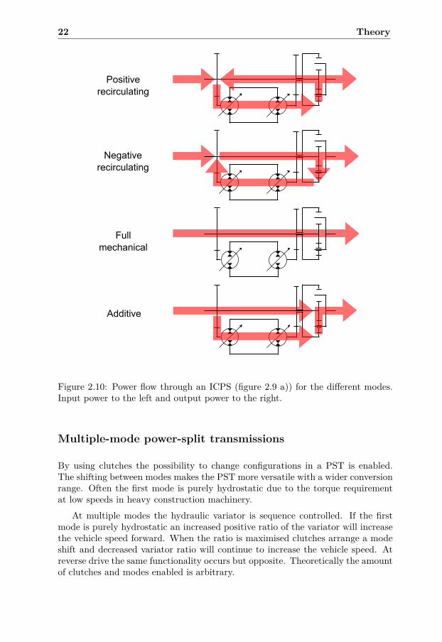
22 Theory
Figure 2.10: Power flow through an ICPS (figure 2.9 a)) for the different modes.Input power to the left and output power to the right.
Multiple-mode power-split transmissions
By using clutches the possibility to change configurations in a PST is enabled.The shifting between modes makes the PST more versatile with a wider conversionrange. Often the first mode is purely hydrostatic due to the torque requirementat low speeds in heavy construction machinery.
At multiple modes the hydraulic variator is sequence controlled. If the firstmode is purely hydrostatic an increased positive ratio of the variator will increasethe vehicle speed forward. When the ratio is maximised clutches arrange a modeshift and decreased variator ratio will continue to increase the vehicle speed. Atreverse drive the same functionality occurs but opposite. Theoretically the amountof clutches and modes enabled is arbitrary.
2.2 Power-split transmissions 23
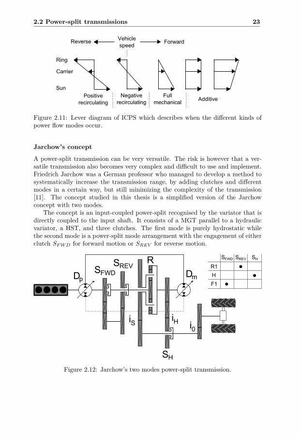
Figure 2.11: Lever diagram of ICPS which describes when the different kinds ofpower flow modes occur.
Jarchow’s concept
A power-split transmission can be very versatile. The risk is however that a ver-satile transmission also becomes very complex and difficult to use and implement.Friedrich Jarchow was a German professor who managed to develop a method tosystematically increase the transmission range, by adding clutches and differentmodes in a certain way, but still minimizing the complexity of the transmission[11]. The concept studied in this thesis is a simplified version of the Jarchowconcept with two modes.
The concept is an input-coupled power-split recognised by the variator that isdirectly coupled to the input shaft. It consists of a MGT parallel to a hydraulicvariator, a HST, and three clutches. The first mode is purely hydrostatic whilethe second mode is a power-split mode arrangement with the engagement of eitherclutch SF W D for forward motion or SREV for reverse motion.
Figure 2.12: Jarchow’s two modes power-split transmission.

24 Theory
Chapter 3
Hardware-in-the-loopSimulation Rig
All hardware tests are carried out in a test rig located in Flumes lab in Linköping.It has a fairly long history in the lab and was built around forty years ago fortesting hydrostatic transmissions. In 2010 the rig was renovated and updatedwith new components such as valves and hydrostatic transmission machines. Thework was part of a master thesis project that took place in the spring of 2010 [12].
After that, several student projects have further developed the rig. In theautumn of 2010, a group of students updated the control system from a xPC targetbased system to a system based on LabVIEW and a Prevas realtime computer [13].This increased the HWIL-simulation performance due to the increased samplingrate. In the autumn of 2013 the rig was updated again in another student project[1]. Controllers for drive side simulation and load side simulation were developedand connections for hydraulic accumulators were added to enable a possibility tosimulate hybrid transmissions.
During the work carried out in this thesis, hydraulic accumulators have beeninstalled in the hydrostatic transmission circuit. These have also been equippedwith on/off valves so that they can be connected or disconnected to the hydrostatictransmission circuit.
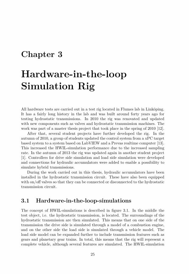
3.1 Hardware-in-the-loop-simulationsThe concept of HWIL-simulations is described in figure 3.1. In the middle thetest object, i.e. the hydrostatic transmission, is located. The surroundings of thehydrostatic transmission are then simulated. This means that on one side of thetransmission the drive side is simulated through a model of a combustion engine,and on the other side the load side is simulated through a vehicle model. Theload side model can be expanded further to include transmission features such asgears and planetary gear trains. In total, this means that the rig will represent acomplete vehicle, although several features are simulated. The HWIL-simulation
25
26 Hardware-in-the-loop Simulation Rig
concept facilitates the engineering procedure, since many different transmissionconcepts can be evaluated for different applications without rebuilding the rig.
Speed/torque
sensor
Speed/torque
sensor
Model of engine Model of gears Model of loadModel of gears
Figure 3.1: Hardware-in-the-loop-simulation rig schematics.
3.2 HardwareSupply systemThe supply system consists of two pumps driven by one 132 kW electric motoreach. A variable pressure relief valve is used to control the supply pressure. Onthe low pressure side, three external boost pumps with a variable pressure reliefvalve are used to maintain the boost pressure.
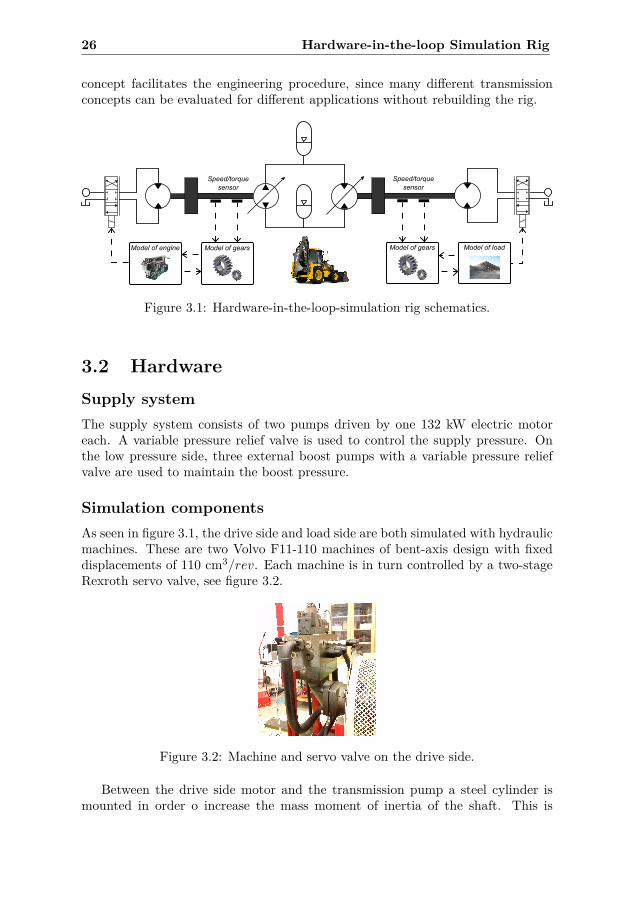
Simulation componentsAs seen in figure 3.1, the drive side and load side are both simulated with hydraulicmachines. These are two Volvo F11-110 machines of bent-axis design with fixeddisplacements of 110 cm3/rev. Each machine is in turn controlled by a two-stageRexroth servo valve, see figure 3.2.
Figure 3.2: Machine and servo valve on the drive side.
Between the drive side motor and the transmission pump a steel cylinder ismounted in order o increase the mass moment of inertia of the shaft. This is
3.2 Hardware 27
supposed to correspond to the inertia of a combustion engine, and also contributesto a smoother speed control. Between the steel cylinder and the transmissionpump, speed and torque sensors are mounted. Through the software feedback thetorque and speed signals can be used to simulate the combustion engine.
Between the transmission motor and the load side simulation hydraulic ma-chine, another steel cylinder is mounted. This cylinder’s inertia is supposed tocorrespond to the load inertia, which in turn is related to the vehicle mass. Thetorque and speed on the shaft between the steel cylinder and the load side hy-draulic machine is available through sensors and are fed back in order to simulatethe load.
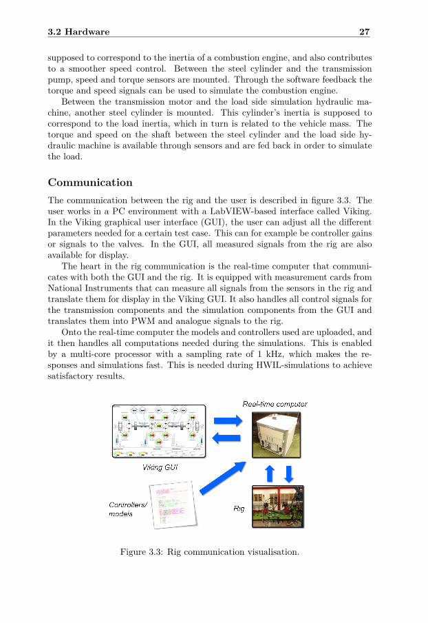
CommunicationThe communication between the rig and the user is described in figure 3.3. Theuser works in a PC environment with a LabVIEW-based interface called Viking.In the Viking graphical user interface (GUI), the user can adjust all the differentparameters needed for a certain test case. This can for example be controller gainsor signals to the valves. In the GUI, all measured signals from the rig are alsoavailable for display.
The heart in the rig communication is the real-time computer that communi-cates with both the GUI and the rig. It is equipped with measurement cards fromNational Instruments that can measure all signals from the sensors in the rig andtranslate them for display in the Viking GUI. It also handles all control signals forthe transmission components and the simulation components from the GUI andtranslates them into PWM and analogue signals to the rig.
Onto the real-time computer the models and controllers used are uploaded, andit then handles all computations needed during the simulations. This is enabledby a multi-core processor with a sampling rate of 1 kHz, which makes the re-sponses and simulations fast. This is needed during HWIL-simulations to achievesatisfactory results.
Figure 3.3: Rig communication visualisation.
28 Hardware-in-the-loop Simulation Rig
Transmission componentsThe hydrostatic transmission consists of an A4VG pump and an A6VM motorfrom BOSCH Rexroth, and are specifically designed for usage in closed hydrostatictransmission circuits, see figure 3.4. Both machines have variable displacementsand the pump has a maximum displacement of 110 cm3/rev while the motor hasa maximum displacement of 150 cm3/rev. The pump is of in-line design and canrealise negative displacement whereas the motor is of the bent-axis type and canrealise displacements between 20% and maximum positive displacement.
Figure 3.4: Pump (left) and motor (right) in the hydrostatic transmission circuit.
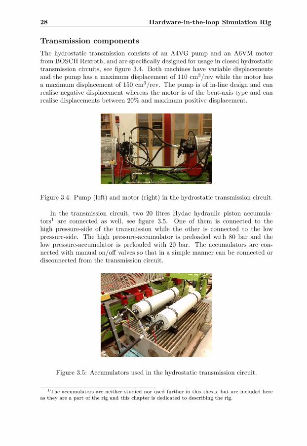
In the transmission circuit, two 20 litres Hydac hydraulic piston accumula-tors1 are connected as well, see figure 3.5. One of them is connected to thehigh pressure-side of the transmission while the other is connected to the lowpressure-side. The high pressure-accumulator is preloaded with 80 bar and thelow pressure-accumulator is preloaded with 20 bar. The accumulators are con-nected with manual on/off valves so that in a simple manner can be connected ordisconnected from the transmission circuit.
Figure 3.5: Accumulators used in the hydrostatic transmission circuit.
1The accumulators are neither studied nor used further in this thesis, but are included hereas they are a part of the rig and this chapter is dedicated to describing the rig.
Chapter 4
Reference Vehicle
In order to obtain results that can be put into context, a reference vehicle isneeded. This vehicle is translated into a model that is implemented into theHWIL-simuation rig. In this project, Volvo CE provides with a reference vehicle.Volvo CE designs and manufactures a large span of construction machinery usedon contruction sites worldwide. Wheel loaders, articulated haulers and excavatorsare examples of products within their range. Here, the studied vehicle is a backhoeloader.
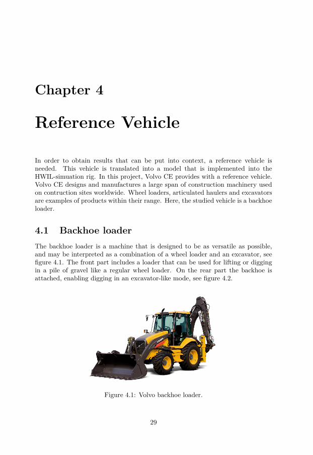
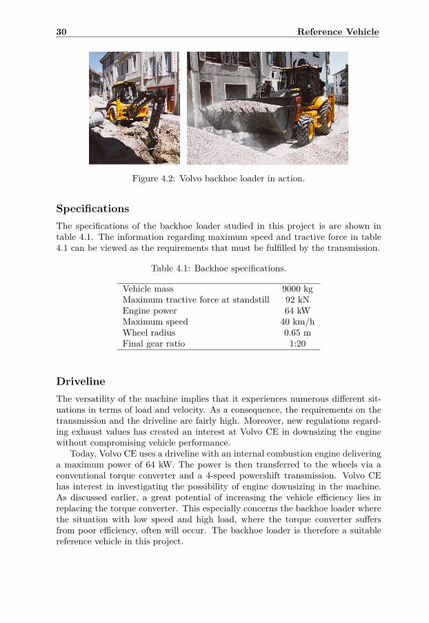
4.1 Backhoe loaderThe backhoe loader is a machine that is designed to be as versatile as possible,and may be interpreted as a combination of a wheel loader and an excavator, seefigure 4.1. The front part includes a loader that can be used for lifting or diggingin a pile of gravel like a regular wheel loader. On the rear part the backhoe isattached, enabling digging in an excavator-like mode, see figure 4.2.
Figure 4.1: Volvo backhoe loader.
29
30 Reference Vehicle
Figure 4.2: Volvo backhoe loader in action.
SpecificationsThe specifications of the backhoe loader studied in this project is are shown intable 4.1. The information regarding maximum speed and tractive force in table4.1 can be viewed as the requirements that must be fulfilled by the transmission.
Table 4.1: Backhoe specifications.
Vehicle mass 9000 kgMaximum tractive force at standstill 92 kNEngine power 64 kWMaximum speed 40 km/hWheel radius 0.65 mFinal gear ratio 1:20
DrivelineThe versatility of the machine implies that it experiences numerous different sit-uations in terms of load and velocity. As a consequence, the requirements on thetransmission and the driveline are fairly high. Moreover, new regulations regard-ing exhaust values has created an interest at Volvo CE in downsizing the enginewithout compromising vehicle performance.
Today, Volvo CE uses a driveline with an internal combustion engine deliveringa maximum power of 64 kW. The power is then transferred to the wheels via aconventional torque converter and a 4-speed powershift transmission. Volvo CEhas interest in investigating the possibility of engine downsizing in the machine.As discussed earlier, a great potential of increasing the vehicle efficiency lies inreplacing the torque converter. This especially concerns the backhoe loader wherethe situation with low speed and high load, where the torque converter suffersfrom poor efficiency, often will occur. The backhoe loader is therefore a suitablereference vehicle in this project.
Chapter 5
Studied TransmissionConcept
Chapters 1-4 have dealt with the background and the conditions under whichthis project is carried out. This chapter covers dimensioning and the resultingtransmission concept that will be investigated in this thesis. The 2-mode Jarchowtransmission is dimensioned so that it fits the reference vehicle and so that it canbe evaluated in the HWIL-simulation rig.
5.1 Dimensioning of power-split transmissionThe dimensioning of a PST mainly concerns the design of the planetary gearconstant and the gear ratios in mechanical parts, as well as the sizes of the machinesin the hydrostatic transmission in order to fulfil a number of requirements. In thisdimensioning the considered configuration, Jarchow’s two modes concept, will bedesigned. The final spur gear, i0, and the radius of the wheels, rwheel, are fixedin the vehicle. In the dimensioning the size of the hydraulic variator units areconsidered given.
The dimensioning is delimited by several requirements. At stand still the ve-hicle has to achieve a maximum tractive force. At desirable mode shift speed theshafts of the clutch which should be activated to change the configuration has tohave synchronised shaft speeds. The gears in the PST must be designed so max-imum vehicle speed can be reached without exceeding limits of the variator unitsin form of maximum speed etc.
Before designing the PST the following parameters are to be given:
• Maximum allowed speed of variator units, nm/p,max.
• Maximum pressure difference in hydraulic variator, ∆p.
• Maximum speed of vehicle, vmax.
• Maximum tractive force, Ftrac.
31
32 Studied Transmission Concept
• Minimum displacement setting of motor, εm,min.
• Speed of internal combustion engine, nICE .
• Vehicle speed where mode shift is desirable, vswitch.
Here, the speed of the ICE is assumed to be constant.
Hydrostatic modeIn the first mode, which is a purely hydrostatic mode, the clutch SH is engagedwhile SF W D and SREV are disengaged. The wheels are directly coupled to thehydraulic motor unit and this mode will from now on be referred to as the hydro-static mode. The gear ratio of the hydrostatic mode gear iH have to be designedso the transmission will be able to deliver maximum tractive force, Ftrac, requiredat stand still:
iH = D2 ∆p ηspur η0
(Ftrac + Fr) i0 rwheel(5.1)
ηspur is the efficiency of the spur gear iH . η0 is the efficiency of the final gear.Fr is the rolling resistance force.
The vehicle velocity in hydrostatic mode is thereby determined by:
vveh = i0 iH rwheel nm (5.2)
Power-split modeThe second mode, which from now on will be referred to as the power-split mode,is arranged by activating either clutch SF W D or SREV depending on directionof motion while clutch SH is deactivated. The forward motion and the reversemotion will behave in same way but with different clutches. Therefore only forwardmotion is analysed below. To be able to switch mode with SF W D the shafts onboth sides of the clutch must be synchronised in the desirable switch speed vswitch.This means that at vswitch both modes correspond to the same motor speed. Inforward mode, this speed is negative at its maximum absolute value. When thevehicle speed increases, the motor velocity increases (becomes more positive) untilit stops and changes direction. At maximum vehicle speed the motor speed ispositive at its maximum absolute value. Thereby, the planetary gear constant Rand the gear ratio iS both depend on the desired mode switch vehicle speed andthe maximum vehicle speed. Assuming mode shift at a certain engine speed, thekinematic relations of the planetary gear and the other gears in the transmissionyields: (5.3) and (5.4):
R = i0 iH nICE rw (−vmax + vswitch)vswitch (vmax + vswitch) (5.3)
is = i0 iH nICE rw(vmax − vswitch) + vswitch (vmax + vswitch)2 i0 nICE rw vswitch
(5.4)
5.2 Dimensioned concept 33
The velocity of the vehicle in power-split mode depends on the hydraulic motorspeed nm, equation (5.5), provided that nsun is equal to nice and constant. Whenthe hydraulic motor speed is zero a full mechanical point occurs. At this operatingpoint, all power is transferred through the mechanical path and the efficiency ofthe PST reaches its maximum.
vveh = i0 iS rwheel (R nm − nICE)R− 1 (5.5)
5.2 Dimensioned conceptThe dimensioning method of the 2-mode Jarchow transmission is described in 5.1and implies a number of input requirements that result in values of gear ratios anda planetary gear constant.
The requirements are set by the reference vehicle and by limitations in thehardware. These conditions are summarised in table 5.1. As seen, the concept isdimensioned for two mode switch speeds, 7 and 10 km/h, which is discussed insection 5.3.
Table 5.1: Numerical input requirements for dimensioning the transmission con-cept. Two switch speeds, 7 and 10 km/h, are tried out.
Parameter ValuenICE 1800 rpm∆pmax 400 barvswitch 7 or 10 km/hvmax 40 km/hFtrac 92 kNηspur 99 %η0 92 %Fr 2 % of normal contact forceMinimum allowed motor displacement setting 0.3Maximum allowed motor speed 3200 rpm
The resulting values of the design parameters are shown in table 5.2.
34 Studied Transmission Concept
Table 5.2: Resulting numerical values of the design parameters in the studiedtransmission concept for two mode switch speeds, 7 and 10 km/h. The maxi-mum motor speed and minimum motor displacement setting that will occur in theconcept are included as well.
Parameter Valuevswitch 7 km/h 10 km/hiH 0.28 0.28iS 1.73 1.55R -0.62 -0.37nm,max 2040 rpm 2915 rpmεm,min 0.53 0.37
In figures 5.1 and 5.2, the realised motor speed and motor/pump displacementsettings versus vehicle speed are shown. As predicted earlier, the maximum motorspeed is reached at mode shift and at maximum vehicle speed. At the same points,the motor displacement setting is at its minimum. The full mechanical point inthe PST mode is found where the motor speed is 0, i.e. approximately 23 km/hfor a mode shift at 7 km/h and 25 km/h for a mode shift at 10 km/h.
Another interesting feature is the rather unusual relation that the the motorspeed decreases when the vehicle speed increases in the power-split mode, whilethe opposite relation is valid in the hydrostatic mode.
5.2 Dimensioned concept 35
−40 −30 −20 −10 0 10 20 30 40
−3000
−2000
−1000
0
1000
2000
3000
Motor speed, vswitch
= 7 km/h
Vehicle velocity [km/h]
Mot
or s
peed
[rpm
]
Motor speedMax allowed motor speed
−50 −40 −30 −20 −10 0 10 20 30 40 50−1
−0.8
−0.6
−0.4
−0.2
0
0.2
0.4
0.6
0.8
1
Displacement settings, vswitch
= 7 km/h
Vehicle speed [km/h]
Dis
plac
emen
t set
ting
PumpMotorMin allowed motor
Figure 5.1: Motor speed and motor/pump displacement settings versus vehiclespeed when mode shift occurs at 7 km/h (i.e. power-split mode is entered at|vveh| > 7 km/h).
36 Studied Transmission Concept
−40 −30 −20 −10 0 10 20 30 40
−3000
−2000
−1000
0
1000
2000
3000
Motor speed, vswitch
= 10 km/h
Vehicle velocity [km/h]
Mot
or s
peed
[rpm
]
Motor speedMax allowed motor speed
−40 −30 −20 −10 0 10 20 30 40−1
−0.8
−0.6
−0.4
−0.2
0
0.2
0.4
0.6
0.8
1
Displacement settings, vswitch
= 10 km/h
Vehicle speed [km/h]
Dis
plac
emen
t set
ting
PumpMotorMin allowed motor
Figure 5.2: Motor speed and motor/pump displacement settings versus vehiclespeed when mode shift occurs at 10 km/h (i.e. power-split mode is entered at|vveh| > 10 km/h).
5.3 Mode shift speed 37
5.3 Mode shift speedAs seen in table 5.2, the gear ratio iH is independent of the mode switch speed.This is because iH is merely determined by the maximum tractive force and themaximum transmission pressure combined with the maximum motor displacement.As a consequence, the maximum motor speed in the concept increases when themode switch speed increases, while the minimum motor displacement setting de-creases. A too high mode shift speed is thereby not preferable due to the lowhydrostatic transmission efficiency at low displacement settings.
However, a mode switch implies a rather non-linear and rapid load changebehaviour on the hydraulic motor. Given that the vehicle is working under a highload and highly varying load in low speeds a low mode switch speed could inflicton the functionality. Furthermore, a high mode switch speed could mean that theclutch SREV is not needed, since the desired maximum speed in reversing modenot is that high as in forward mode, which implies savings in manufacturing costs.
As seen in figures 5.1 and 5.2, mode shift speeds of 10 km/h and 7 km/h areboth feasible solutions since the motor speeds and motor displacement settings arewithin the set limits. Further on in this thesis however, the concept with a modeswitch speed of 7 km/h will be analysed. Partly to avoid too small displacementvalues, but primarily to avoid too high motor speeds in the HWIL-simulation rig.
5.4 Comparison of conceptsOverall a transmission for heavy construction machinery needs to fulfil require-ments regarding tractive force at stand still and vehicle speed. These two require-ments sets the corner points in a force-velocity graph of the transmission concept.By comparing force-velocity graphs for both the torque converter and the power-split transmission a better understanding of strengths and weaknesses is obtained.The requirements that must be fulfilled for the application is seen in table 5.3.
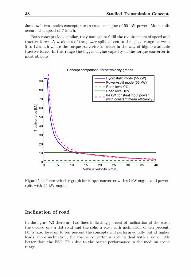
RoadingFigure 5.3 shows the force the both transmissions is able to perform at a certainvehicle speed for a roading case. Roading refers to a transport mode where all theICE power is consumed by the transmission compared with a loading case whereexternal hydraulic circuits consumes torque continuously from the engine. Thetorque converter use an ICE with 64 kW power and a power shift gearbox with4 gears. The data used for the torque converter is derived from a constant meanefficiency and forms a constant power curve. The power-split concept, which is
Table 5.3: Requirement of backhoe application.
Maximum tractive force at standstill 92 KNMaximum speed 40 km/h
38 Studied Transmission Concept
Jarchow’s two modes concept, uses a smaller engine of 55 kW power. Mode shiftoccurs at a speed of 7 km/h.
Both concepts look similar, they manage to fulfil the requirements of speed andtractive force. A weakness of the power-split is seen in the speed range between5 to 12 km/h where the torque converter is better in the way of higher availabletractive force. In this range the bigger engine capacity of the torque converter ismost obvious.
0 5 10 15 20 25 30 35 400
10
20
30
40
50
60
70
80
90
Tra
ctive f
orc
e [
kN
]
Vehicle velocity [km/h]
Concept comparison, force velocity graphs
Hydrostatic mode (55 kW)
Power split mode (55 kW)
Road level 0%
Road level 10%
64 kW constant input power(with constant mean efficiency)
Figure 5.3: Force-velocity graph for torque converter with 64 kW engine and power-split with 55 kW engine.
Inclination of road
In the figure 5.3 there are two lines indicating percent of inclination of the road,the dashed one a flat road and the solid a road with inclination of ten percent.For a road level up to ten percent the concepts will perform equally but at higherloads, more inclination, the torque converter is able to deal with a slope littlebetter than the PST. This due to the better performance in the medium speedrange.
5.4 Comparison of concepts 39
Minor conclusionTo summarise the concepts performance the PST will fulfil the requirements oftractive force and maximum speed with a smaller combustion engine while thetorque converter uses a bigger engine for same work. The torque converter willhowever be able to perform better at the medium speed range, 5 to 20 km/h,where the PST maybe will feel weak in comparison. This could be interpreted asan issue as it intrudes on the functionality. Still, in the downsizing procedure, therequirements regarding maximum tractive force and maximum vehicle speed aredominant which implies that this issue can be neglected here.

40 Studied Transmission Concept
Chapter 6
Modelling and Simulation
As emphasised earlier, system simulations is a very useful tool in the developmentof control algorithms and for an increased understanding of the system. Thischapter covers the development and evaluation of the models used in order toperform the simulations. All models are implemented in Hopsan, except for theHWIL-simulation model which is implemented in Simulink.
6.1 HopsanHopsan is a system simulation tool developed at Flumes on Linköping Univer-sity [2]. The project has a long history, starting as early as 1977. Since then,it has changed and evolved through academic research and industrial/academiccollaborations. In 2009 a PhD project launched, where the Hopsan platform wascompletely updated and rebuilt. The process is still ongoing, but so far it hasresulted in a versatile and user friendly simulation software that is used in bothindustrial applications and in the courses within fluid power systems at LinköpingUniversity.
The distinguishing feature of Hopsan, that separates it from most other simula-tion packages, is the use of decentralised solvers compared to the more commonlyused centralised solvers. This is enabled by the usage of transmission line mod-elling (TLM). This method uses time delays within the model to simulate thephysical time delays present in a real system, e.g. the time it takes for a pressurewave to propagate in a pipe. In turn, the model components are separated fromeach other in time which implies that different parts of the model can be simulatedsimultaneously. This combined with the fixed step solver creates a linear relation-ship between simulation time and model size, and a possibility to significantlydecrease simulation time by using processors with multiple cores [14].
Furthermore, the hopsan models can be compiled into both Matlab/Simulink-and LabVIEW-formats. This means that the different controllers easily can bedeveloped in Simulink and tested in simulations, and then directly implementedin the test rig.
41
42 Modelling and Simulation
6.2 Hydrostatic transmission
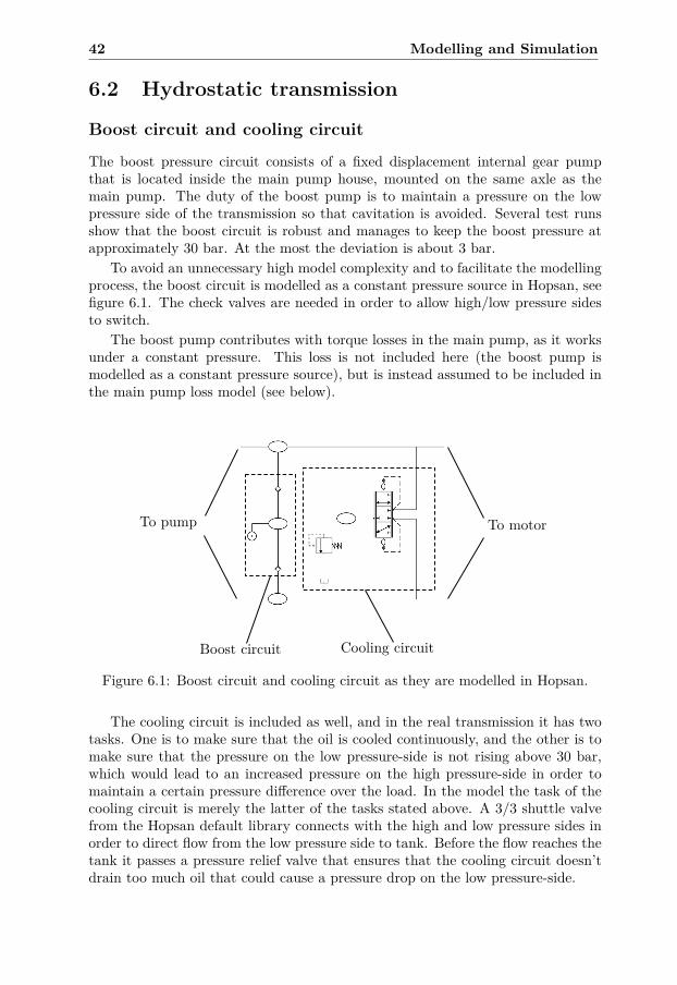
Boost circuit and cooling circuit
The boost pressure circuit consists of a fixed displacement internal gear pumpthat is located inside the main pump house, mounted on the same axle as themain pump. The duty of the boost pump is to maintain a pressure on the lowpressure side of the transmission so that cavitation is avoided. Several test runsshow that the boost circuit is robust and manages to keep the boost pressure atapproximately 30 bar. At the most the deviation is about 3 bar.
To avoid an unnecessary high model complexity and to facilitate the modellingprocess, the boost circuit is modelled as a constant pressure source in Hopsan, seefigure 6.1. The check valves are needed in order to allow high/low pressure sidesto switch.
The boost pump contributes with torque losses in the main pump, as it worksunder a constant pressure. This loss is not included here (the boost pump ismodelled as a constant pressure source), but is instead assumed to be included inthe main pump loss model (see below).
To pump To motor
Boost circuit Cooling circuit
Figure 6.1: Boost circuit and cooling circuit as they are modelled in Hopsan.
The cooling circuit is included as well, and in the real transmission it has twotasks. One is to make sure that the oil is cooled continuously, and the other is tomake sure that the pressure on the low pressure-side is not rising above 30 bar,which would lead to an increased pressure on the high pressure-side in order tomaintain a certain pressure difference over the load. In the model the task of thecooling circuit is merely the latter of the tasks stated above. A 3/3 shuttle valvefrom the Hopsan default library connects with the high and low pressure sides inorder to direct flow from the low pressure side to tank. Before the flow reaches thetank it passes a pressure relief valve that ensures that the cooling circuit doesn’tdrain too much oil that could cause a pressure drop on the low pressure-side.
6.2 Hydrostatic transmission 43
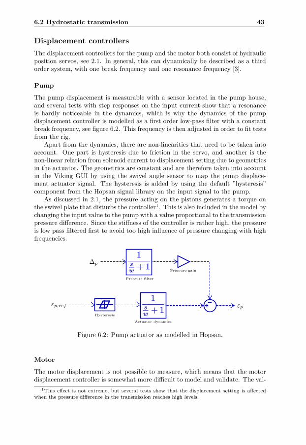
Displacement controllersThe displacement controllers for the pump and the motor both consist of hydraulicposition servos, see 2.1. In general, this can dynamically be described as a thirdorder system, with one break frequency and one resonance frequency [3].
Pump
The pump displacement is measurable with a sensor located in the pump house,and several tests with step responses on the input current show that a resonanceis hardly noticeable in the dynamics, which is why the dynamics of the pumpdisplacement controller is modelled as a first order low-pass filter with a constantbreak frequency, see figure 6.2. This frequency is then adjusted in order to fit testsfrom the rig.
Apart from the dynamics, there are non-linearities that need to be taken intoaccount. One part is hysteresis due to friction in the servo, and another is thenon-linear relation from solenoid current to displacement setting due to geometricsin the actuator. The geometrics are constant and are therefore taken into accountin the Viking GUI by using the swivel angle sensor to map the pump displace-ment actuator signal. The hysteresis is added by using the default ”hysteresis”component from the Hopsan signal library on the input signal to the pump.
As discussed in 2.1, the pressure acting on the pistons generates a torque onthe swivel plate that disturbs the controller1. This is also included in the model bychanging the input value to the pump with a value proportional to the transmissionpressure difference. Since the stiffness of the controller is rather high, the pressureis low pass filtered first to avoid too high influence of pressure changing with highfrequencies.
∆p
Hysteresis
Actuator dynamics
εp,ref εp
Pressure filter
Pressure gain
Figure 6.2: Pump actuator as modelled in Hopsan.
Motor
The motor displacement is not possible to measure, which means that the motordisplacement controller is somewhat more difficult to model and validate. The val-
1This effect is not extreme, but several tests show that the displacement setting is affectedwhen the pressure difference in the transmission reaches high levels.
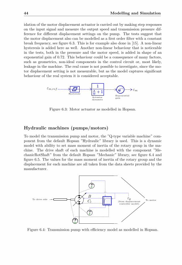
44 Modelling and Simulation
idation of the motor displacement actuator is carried out by making step responseson the input signal and measure the output speed and transmission pressure dif-ference for different displacement settings on the pump. The tests suggest thatthe motor displacement also can be modelled as a first order filter with a constantbreak frequency, see figure 6.3. This is for example also done in [15]. A non-linearhysteresis is added here as well. Another non-linear behaviour that is noticeablein the tests, both in the pressure and the motor speed, is added in shape of anexponential gain of 0.72. This behaviour could be a consequence of many factors,such as geometrics, non-ideal components in the control circuit or, most likely,leakage in the machine. The real cause is not possible to investigate, since the mo-tor displacement setting is not measurable, but as the model captures significantbehaviour of the real system it is considered acceptable.
Hysteresis
Actuatordynamics
εm,ref
Exponentialgain
εm
Figure 6.3: Motor actuator as modelled in Hopsan.
Hydraulic machines (pumps/motors)
To model the transmission pump and motor, the ”Q-type variable machine” com-ponent from the default Hopsan ”Hydraulic” library is used. This is a dynamicmodel with ability to set mass moment of inertia of the rotary group in the ma-chine. The drive shaft of each machine is modelled with the component ”Me-chanicRotShaft” from the default Hopsan ”Mechanic” library, see figure 6.4 andfigure 6.5. The values for the mass moment of inertia of the rotary group and thedisplacement for each machine are all taken from the data sheets provided by themanufacturer.
εp(from displacementcontroller model)
BCl
To motorTo drive side
Figure 6.4: Transmission pump with efficiency model as modelled in Hopsan.
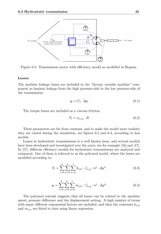
6.2 Hydrostatic transmission 45
εm(from displacementcontroller model)
BCl
To pump To load
Figure 6.5: Transmission motor with efficiency model as modelled in Hopsan.
Losses
The machine leakage losses are included in the ”Q-type variable machine” com-ponent as laminar leakage from the high pressure-side to the low pressure-side ofthe transmission:
ql = Cl ·∆p (6.1)
The torque losses are included as a viscous friction:
Tl = nm,p ·B (6.2)
These parameters are far from constant, and to make the model more realisticthey are varied during the simulation, see figures 6.5 and 6.4, according to lossmodels.
Losses in hydrostatic transmissions is a well known issue, and several modelshave been developed and investigated over the years, see for example [16] and [17].In [17], different efficiency models for hydrostatic transmissions are analysed andcompared. One of them is referred to as the polymod model, where the losses aremodelled according to:
Tl =p∑
i=0
q∑j=0
r∑u=0
kiju · εim,p · nj ·∆pu (6.3)
ql =p∑
i=0
q∑j=0
r∑u=0
miju · εim,p · nj ·∆pu (6.4)
The polymod concept suggests that all losses can be related to the machinespeed, pressure difference and the displacement setting. A high number of termswith many different exponential factors are included, and then the constants kiju
and miju are fitted to data using linear regression.
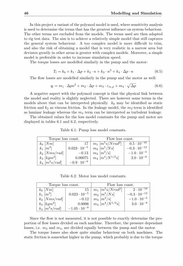
46 Modelling and Simulation
In this project a variant of the polymod model is used, where sensitivity analysisis used to determine the terms that has the greatest influence on system behaviour.The other terms are excluded from the models. The terms used are then adaptedto rig test data. The aim is to achieve a relatively simple model that still capturesthe general system behaviour. A too complex model is more difficult to trim,and also the risk of obtaining a model that is very realistic in a narrow area butdeviates greatly in other areas is greater with complex models. Moreover, a simplemodel is preferable in order to increase simulation speed.
The torque losses are modelled similarly in the pump and the motor:
Tl = k0 + k1 ·∆p+ k2 · n+ k3 · n2 + k4 ·∆p · n (6.5)The flow losses are modelled similarly in the pump and the motor as well:
ql = m1 ·∆pn2 +m2 ·∆p+m3 · εm,p +m4 ·√
∆p (6.6)
A negative aspect with the polymod concept is that the physical link betweenthe model and reality is slightly neglected. There are however some terms in themodels above that can be interpreted physically. k0 may be identified as staticfriction and k2 as viscous friction. In the leakage model, the m2-term is identifiedas laminar leakage whereas the m4 term can be interpreted as turbulent leakage.
The obtained values for the loss model constants for the pump and motor aredisplayed in tables 6.1 and 6.2, respectively.
Table 6.1: Pump loss model constants.
Torque loss const. Flow loss const.k0 [Nm] 17 m1 [m5s/Nrad2] 0.5 · 10−16
k1 [m3] 0.023 · 10−5 m2 [m5/Ns] −0.3 · 10−12
k2 [Nms/rad] −0.13 m3 [m3/s] −1.0 · 10−5
k3 [kgm2] 0.00075 m4 [m4/N1/2s] 3.0 · 10−8
k4 [m3s/rad] −0.9 · 10−9
Table 6.2: Motor loss model constants.
Torque loss const. Flow loss const.k0 [Nm] 15 m1 [m5s/Nrad2] 2 · 10−16
k1 [m3] 0.023 · 10−5 m2 [m5/Ns] −0.3 · 10−12
k2 [Nms/rad] −0.12 m3 [m3/s] −1.0 · 10−5
k3 [kgm2] 0.0006 m4 [m4/N1/2s] 3.0 · 10−8
k4 [m3s/rad] −1.05 · 10−9
Since the flow is not measured, it is not possible to exactly determine the pro-portion of flow losses divided on each machine. Therefore, the pressure dependantlosses, i.e. m2 and m4, are divided equally between the pump and the motor.
The torque losses also show quite similar behaviour on both machines. Thestatic friction is somewhat higher in the pump, which probably is due to the torque
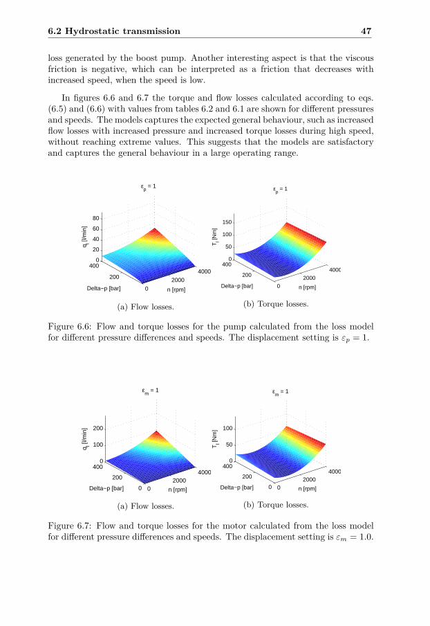
6.2 Hydrostatic transmission 47
loss generated by the boost pump. Another interesting aspect is that the viscousfriction is negative, which can be interpreted as a friction that decreases withincreased speed, when the speed is low.
In figures 6.6 and 6.7 the torque and flow losses calculated according to eqs.(6.5) and (6.6) with values from tables 6.2 and 6.1 are shown for different pressuresand speeds. The models captures the expected general behaviour, such as increasedflow losses with increased pressure and increased torque losses during high speed,without reaching extreme values. This suggests that the models are satisfactoryand captures the general behaviour in a large operating range.
0
2000
4000200
4000
20
40
60
80
n [rpm]
εp = 1
Delta−p [bar]
q l [l/m
in]
(a) Flow losses.
0
2000
4000200
4000
50
100
150
n [rpm]
εp = 1
Delta−p [bar]
Tl [N
m]
(b) Torque losses.
Figure 6.6: Flow and torque losses for the pump calculated from the loss modelfor different pressure differences and speeds. The displacement setting is εp = 1.
02000
4000
0
200
4000
100
200
n [rpm]
εm
= 1
Delta−p [bar]
q l [l/m
in]
(a) Flow losses.
02000
4000
0
200
4000
50
100
n [rpm]
εm
= 1
Delta−p [bar]
Tl [N
m]
(b) Torque losses.
Figure 6.7: Flow and torque losses for the motor calculated from the loss modelfor different pressure differences and speeds. The displacement setting is εm = 1.0.
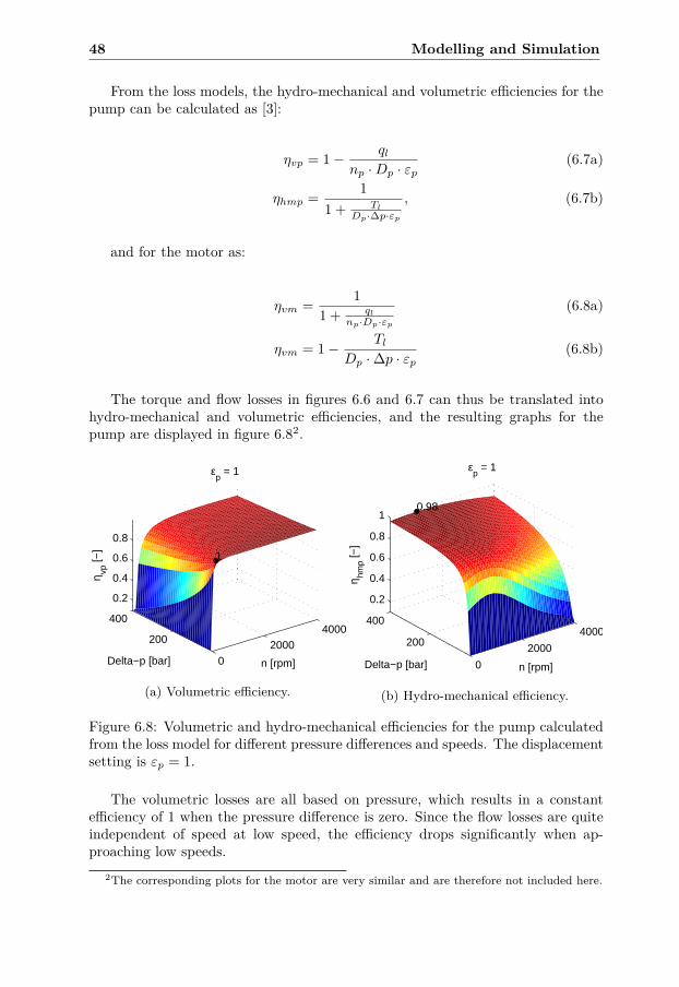
48 Modelling and Simulation
From the loss models, the hydro-mechanical and volumetric efficiencies for thepump can be calculated as [3]:
ηvp = 1− ql
np ·Dp · εp(6.7a)
ηhmp = 11 + Tl
Dp·∆p·εp
, (6.7b)
and for the motor as:
ηvm = 11 + ql
np·Dp·εp
(6.8a)
ηvm = 1− Tl
Dp ·∆p · εp(6.8b)
The torque and flow losses in figures 6.6 and 6.7 can thus be translated intohydro-mechanical and volumetric efficiencies, and the resulting graphs for thepump are displayed in figure 6.82.
02000
4000200
400
0.2
0.4
0.6
0.8
n [rpm]
εp = 1
1
Delta−p [bar]
η vp [−
]
(a) Volumetric efficiency.
0
2000
4000200
400
0.2
0.4
0.6
0.8
1
n [rpm]
εp = 1
Delta−p [bar]
0.98
η hmp [−
]
(b) Hydro-mechanical efficiency.
Figure 6.8: Volumetric and hydro-mechanical efficiencies for the pump calculatedfrom the loss model for different pressure differences and speeds. The displacementsetting is εp = 1.
The volumetric losses are all based on pressure, which results in a constantefficiency of 1 when the pressure difference is zero. Since the flow losses are quiteindependent of speed at low speed, the efficiency drops significantly when ap-proaching low speeds.
2The corresponding plots for the motor are very similar and are therefore not included here.
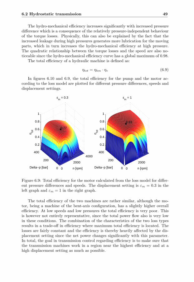
6.2 Hydrostatic transmission 49
The hydro-mechanical efficiency increases significantly with increased pressuredifference which is a consequence of the relatively pressure-independent behaviourof the torque losses. Physically, this can also be explained by the fact that theincreased leakage during high pressures generates more lubrication for the movingparts, which in turn increases the hydro-mechanical efficiency at high pressure.The quadratic relationship between the torque losses and the speed are also no-ticeable since the hydro-mechanical efficiency curve has a global maximum of 0.98.
The total efficiency of a hydraulic machine is defined as:
ηtot = ηhm · ηv (6.9)
In figures 6.10 and 6.9, the total efficiency for the pump and the motor ac-cording to the loss model are plotted for different pressure differences, speeds anddisplacement settings.
0
2000
4000
0
200
400
0.2
0.4
0.6
0.8
1
n [rpm]
εm
= 0.3
0.77
Delta−p [bar]
η tot
0
2000
0
200
400
0.2
0.4
0.6
0.8
1
n [rpm]
εm
= 1
0.93
Delta−p [bar]
η tot
Figure 6.9: Total efficiency for the motor calculated from the loss model for differ-ent pressure differences and speeds. The displacement setting is εm = 0.3 in theleft graph and εm = 1 in the right graph.
The total efficiency of the two machines are rather similar, although the mo-tor, being a machine of the bent-axis configuration, has a slightly higher overallefficiency. At low speeds and low pressures the total efficiency is very poor. Thisis however not entirely representative, since the total power flow also is very lowin these conditions. The combination of the characteristics of the two loss typesresults in a trade-off in efficiency where maximum total efficiency is located. Thelosses are fairly constant and the efficiency is thereby heavily affected by the dis-placement setting since the net power changes significantly with this parameter.In total, the goal in transmission control regarding efficiency is to make sure thatthe transmission machines work in a region near the highest efficiency and at ahigh displacement setting as much as possible.
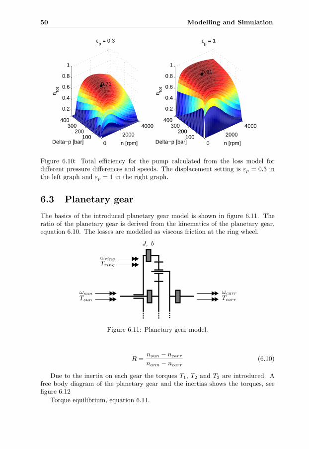
50 Modelling and Simulation
0
2000
4000
100200
300400
0.2
0.4
0.6
0.8
1
n [rpm]
εp = 0.3
0.71
Delta−p [bar]
η tot
0
2000
4000
100200
300400
0.2
0.4
0.6
0.8
1
n [rpm]
εp = 1
0.91
Delta−p [bar]
η tot
Figure 6.10: Total efficiency for the pump calculated from the loss model fordifferent pressure differences and speeds. The displacement setting is εp = 0.3 inthe left graph and εp = 1 in the right graph.
6.3 Planetary gearThe basics of the introduced planetary gear model is shown in figure 6.11. Theratio of the planetary gear is derived from the kinematics of the planetary gear,equation 6.10. The losses are modelled as viscous friction at the ring wheel.
ωsunTsun
ωcarrTcarr
ωringTring
J, b
Figure 6.11: Planetary gear model.
R = nsun − ncarr
nann − ncarr(6.10)
Due to the inertia on each gear the torques T1, T2 and T3 are introduced. Afree body diagram of the planetary gear and the inertias shows the torques, seefigure 6.12
Torque equilibrium, equation 6.11.
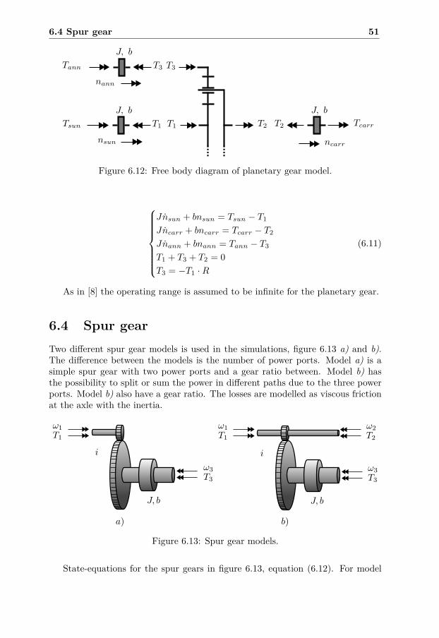
6.4 Spur gear 51
nsun
Tsun
ncarr
Tcarr
nann
Tann
J, b
J, b
T3
T1 T2
J, b
ωsunTsun
ωcarrTcarr
ωannTann
J, b
J, b
ω3T3
ω1T1
ω2T2
J, b
T3
T1 T2
Figure 6.12: Free body diagram of planetary gear model.
Jnsun + bnsun = Tsun − T1
Jncarr + bncarr = Tcarr − T2
Jnann + bnann = Tann − T3
T1 + T3 + T2 = 0T3 = −T1 ·R
(6.11)
As in [8] the operating range is assumed to be infinite for the planetary gear.
6.4 Spur gearTwo different spur gear models is used in the simulations, figure 6.13 a) and b).The difference between the models is the number of power ports. Model a) is asimple spur gear with two power ports and a gear ratio between. Model b) hasthe possibility to split or sum the power in different paths due to the three powerports. Model b) also have a gear ratio. The losses are modelled as viscous frictionat the axle with the inertia.
ω1T1
ω2T2
ω3T3
ω1T1
ω3T3
J, b J, b
ii
a) b)
Figure 6.13: Spur gear models.
State-equations for the spur gears in figure 6.13, equation (6.12). For model
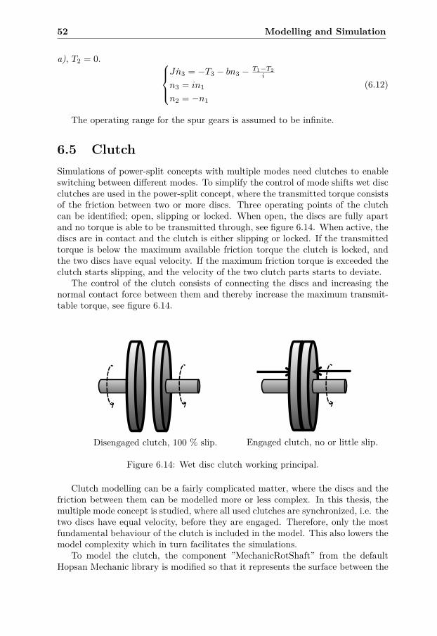
52 Modelling and Simulation
a), T2 = 0. Jn3 = −T3 − bn3 − T1−T2
i
n3 = in1
n2 = −n1
(6.12)
The operating range for the spur gears is assumed to be infinite.
6.5 ClutchSimulations of power-split concepts with multiple modes need clutches to enableswitching between different modes. To simplify the control of mode shifts wet discclutches are used in the power-split concept, where the transmitted torque consistsof the friction between two or more discs. Three operating points of the clutchcan be identified; open, slipping or locked. When open, the discs are fully apartand no torque is able to be transmitted through, see figure 6.14. When active, thediscs are in contact and the clutch is either slipping or locked. If the transmittedtorque is below the maximum available friction torque the clutch is locked, andthe two discs have equal velocity. If the maximum friction torque is exceeded theclutch starts slipping, and the velocity of the two clutch parts starts to deviate.
The control of the clutch consists of connecting the discs and increasing thenormal contact force between them and thereby increase the maximum transmit-table torque, see figure 6.14.
Disengaged clutch, 100 % slip. Engaged clutch, no or little slip.
Figure 6.14: Wet disc clutch working principal.
Clutch modelling can be a fairly complicated matter, where the discs and thefriction between them can be modelled more or less complex. In this thesis, themultiple mode concept is studied, where all used clutches are synchronized, i.e. thetwo discs have equal velocity, before they are engaged. Therefore, only the mostfundamental behaviour of the clutch is included in the model. This also lowers themodel complexity which in turn facilitates the simulations.
To model the clutch, the component ”MechanicRotShaft” from the defaultHopsan Mechanic library is modified so that it represents the surface between the

6.5 Clutch 53
clutch discs. This means that the inertia of the discs are assumed to be included inthe other components, such as the spur gears. The modification of the componentconsists of limiting the maximum transmittable torque between the two portsto a maximum friction torque. When the clutch is engaged the normal contactforce, and thereby the friction, between the discs is increased. The engaging anddisengaging of the modelled clutch is thereby done by increasing and decreasingthe maximum friction torque. For more information regarding the implementationof the clutch equations, see appendix.
ExampleTo test the clutch function, a simple test model can be studied. A simple systemin Hopsan with a clutch and a rotational inertia with viscous friction is shown infigure 6.15, and the resulting graph is shown in figure 6.16. The simulation startswith the clutch disengaged and with constant speed of 500 r.p.m. on the left sideof the clutch. At 1 second the clutch is engaged by ramping the maximum frictiontorque from 0 to 600 Nm during 1 second. The inertia starts to accelerate until itreaches the same speed as the left side of the clutch. At 3 seconds a disturbance isadded in shape of a braking torque step with a magnitude of 200 Nm on the rightside of the rotational inertia. Since the maximum friction torque in the clutch istoo small to transmit the torque needed at the current speed, the clutch starts toslip and the inertia slows down.
500 r.p.m.
Clutch
Disturbance torque
Max friction torque
Figure 6.15: Small example system with a clutch in Hopsan.
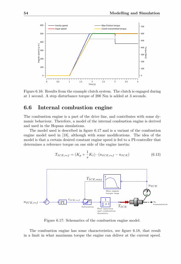
54 Modelling and Simulation
Figure 6.16: Results from the example clutch system. The clutch is engaged duringat 1 second. A step disturbance torque of 200 Nm is added at 3 seconds.
6.6 Internal combustion engineThe combustion engine is a part of the drive line, and contributes with some dy-namic behaviour. Therefore, a model of the internal combustion engine is derivedand used in the Hopsan simulations.
The model used is described in figure 6.17 and is a variant of the combustionengine model used in [18], although with some modifications. The idea of themodel is that a certain desired constant engine speed is fed to a PI-controller thatdetermines a reference torque on one side of the engine inertia:
TICE,ref = (Kp + 1sKI) · (nICE,ref − nICE) (6.13)
Fuel injectionand combustiondynamics
TICE,refnICE,ref PI
Saturation
Max enginetorque map
Totransmission
TICE,max
nICE
TICE
Figure 6.17: Schematics of the combustion engine model.
The combustion engine has some characteristics, see figure 6.18, that resultin a limit in what maximum torque the engine can deliver at the current speed.
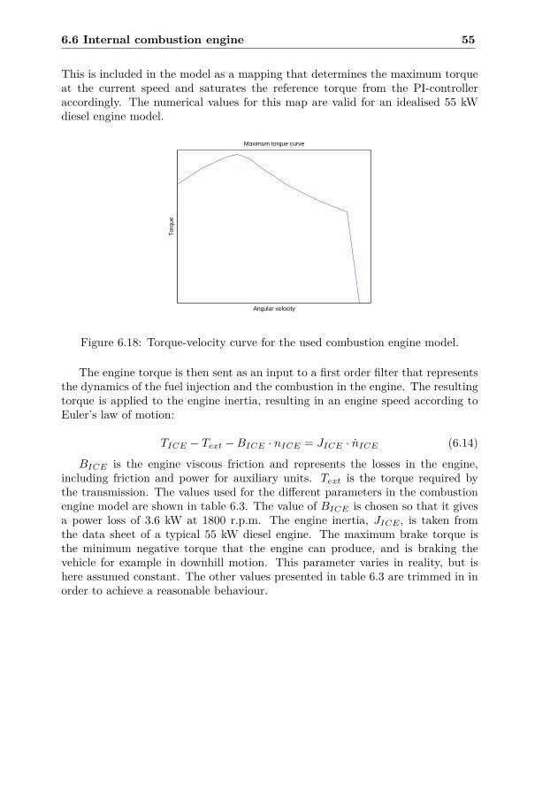
6.6 Internal combustion engine 55
This is included in the model as a mapping that determines the maximum torqueat the current speed and saturates the reference torque from the PI-controlleraccordingly. The numerical values for this map are valid for an idealised 55 kWdiesel engine model.
Maximum torque curve
Angular velocity
Tor
que
Figure 6.18: Torque-velocity curve for the used combustion engine model.
The engine torque is then sent as an input to a first order filter that representsthe dynamics of the fuel injection and the combustion in the engine. The resultingtorque is applied to the engine inertia, resulting in an engine speed according toEuler’s law of motion:
TICE − Text −BICE · nICE = JICE · nICE (6.14)
BICE is the engine viscous friction and represents the losses in the engine,including friction and power for auxiliary units. Text is the torque required bythe transmission. The values used for the different parameters in the combustionengine model are shown in table 6.3. The value of BICE is chosen so that it givesa power loss of 3.6 kW at 1800 r.p.m. The engine inertia, JICE , is taken fromthe data sheet of a typical 55 kW diesel engine. The maximum brake torque isthe minimum negative torque that the engine can produce, and is braking thevehicle for example in downhill motion. This parameter varies in reality, but ishere assumed constant. The other values presented in table 6.3 are trimmed in inorder to achieve a reasonable behaviour.
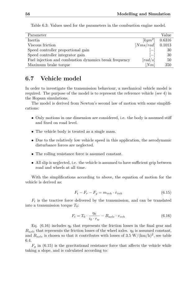
56 Modelling and Simulation
Table 6.3: Values used for the parameters in the combustion engine model.
Parameter ValueInertia [kgm2] 0.6316Viscous friction [Nms/rad] 0.1013Speed controller proportional gain [−] 30Speed controller integrator gain [−] 30Fuel injection and combustion dynamics break frequency [rad/s] 50Maximum brake torque [Nm] 350
6.7 Vehicle modelIn order to investigate the transmission behaviour, a mechanical vehicle model isrequired. The purpose of the model is to represent the reference vehicle (see 4) inthe Hopsan simulations.
The model is derived from Newton’s second law of motion with some simplifi-cations:
• Only motions in one dimension are considered, i.e. the body is assumed stiffand fixed on road level.
• The vehicle body is treated as a single mass.
• Due to the relatively low vehicle speed in this application, the aerodynamicdisturbance forces are neglected.
• The rolling resistance force is assumed constant.
• All slip is neglected, i.e. the vehicle is assumed to have sufficient grip betweenroad and wheels at all time.
With the simplifications according to above, the equation of motion for thevehicle is derived as:
Ft − Fr − Fg = mveh · vveh (6.15)
Ft is the tractive force delivered by the transmission, and can be translatedinto a transmission torque T0:
Ft = T0 ·η0
i0 · rw−Baxle · vveh (6.16)
Eq. (6.16) includes η0 that represents the friction losses in the final gear andBaxle that represents the friction losses of the wheel axles. η0 is assumed constant,and Baxle is chosen so that it contributes with losses of 3.5 W/(km/h)2, see table6.4.
Fg in (6.15) is the gravitational resistance force that affects the vehicle whiletaking a slope, and is calculated according to:
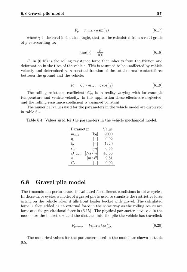
6.8 Gravel pile model 57
Fg = mveh · g sin(γ) (6.17)
where γ is the road inclination angle, that can be calculated from a road gradeof p % according to:
tan(γ) = p
100 (6.18)
Fr in (6.15) is the rolling resistance force that inherits from the friction anddeformation in the tires of the vehicle. This is assumed to be unaffected by vehiclevelocity and determined as a constant fraction of the total normal contact forcebetween the ground and the vehicle:
Fr = Cr ·mveh · g cos(γ) (6.19)
The rolling resistance coefficient, Cr, is in reality varying with for exampletemperature and vehicle velocity. In this application these effects are neglected,and the rolling resistance coefficient is assumed constant.
The numerical values used for the parameters in the vehicle model are displayedin table 6.4.
Table 6.4: Values used for the parameters in the vehicle mechanical model.
Parameter Valuemveh [kg] 9000η0 [−] 0.92i0 [−] 1/20rw [m] 0.65Baxle [Ns/m] 45.36g [m/s2] 9.81Cr [−] 0.02
6.8 Gravel pile modelThe transmission performance is evaluated for different conditions in drive cycles.In those drive cycles, a model of a gravel pile is used to simulate the restrictive forceacting on the vehicle when it fills front loader bucket with gravel. The calculatedforce is then added as an external force in the same way as the rolling resistanceforce and the gravitational force in (6.15). The physical parameters involved in themodel are the bucket size and the distance into the pile the vehicle has travelled:
Fgravel = Vbucketk3xk4veh (6.20)
The numerical values for the parameters used in the model are shown in table6.5.
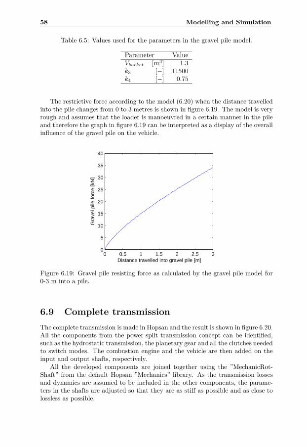
58 Modelling and Simulation
Table 6.5: Values used for the parameters in the gravel pile model.
Parameter ValueVbucket [m3] 1.3k3 [−] 11500k4 [−] 0.75
The restrictive force according to the model (6.20) when the distance travelledinto the pile changes from 0 to 3 metres is shown in figure 6.19. The model is veryrough and assumes that the loader is manoeuvred in a certain manner in the pileand therefore the graph in figure 6.19 can be interpreted as a display of the overallinfluence of the gravel pile on the vehicle.
0 0.5 1 1.5 2 2.5 30
5
10
15
20
25
30
35
40
Distance travelled into gravel pile [m]
Gra
vel p
ile fo
rce
[kN
]
Figure 6.19: Gravel pile resisting force as calculated by the gravel pile model for0-3 m into a pile.
6.9 Complete transmissionThe complete transmission is made in Hopsan and the result is shown in figure 6.20.All the components from the power-split transmission concept can be identified,such as the hydrostatic transmission, the planetary gear and all the clutches neededto switch modes. The combustion engine and the vehicle are then added on theinput and output shafts, respectively.
All the developed components are joined together using the ”MechanicRot-Shaft” from the default Hopsan ”Mechanics” library. As the transmission lossesand dynamics are assumed to be included in the other components, the parame-ters in the shafts are adjusted so that they are as stiff as possible and as close tolossless as possible.

6.9 Complete transmission 59
The inputs to the model is the pump and motor displacement settings, theengine reference speed and signals to the clutches.
The model in figure 6.20 is compiled into a S-function, so that the it canbe simulated from Simulink, where all the inputs and outputs of the model areavailable. The control algorithms are then developed and evaluated in Simulink.
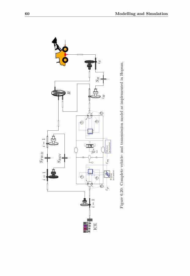
60 Modelling and Simulation
Pump
actuator
Motor
actuator
ICE
SF
WD
SR
EV
SH
i Si H
i=
1i
=1
i=
1
R
ε pε m
Figu
re6.20:Com
pletevehicle-
andtran
smiss
ionmod
elas
implem
entedin
Hop
san.
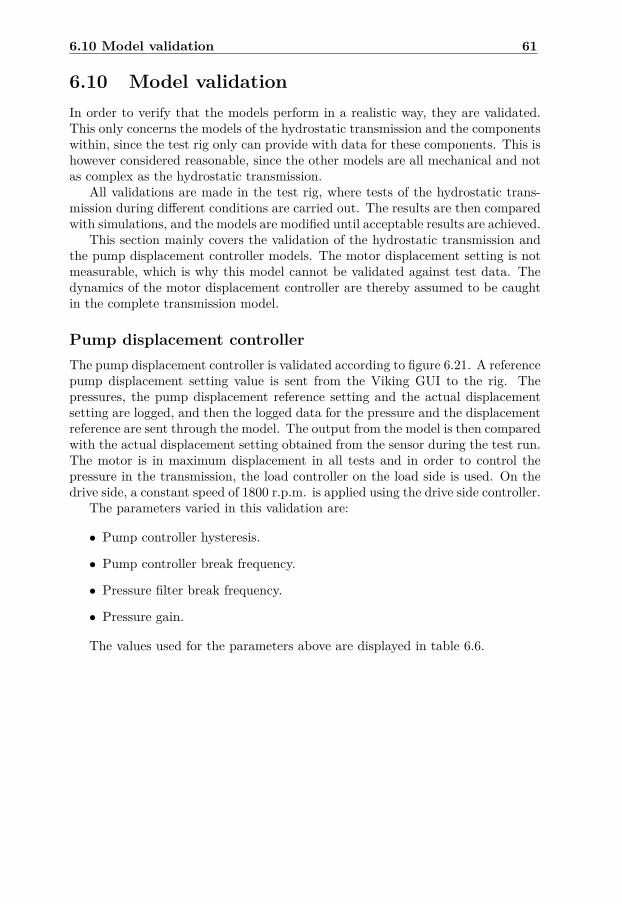
6.10 Model validation 61
6.10 Model validationIn order to verify that the models perform in a realistic way, they are validated.This only concerns the models of the hydrostatic transmission and the componentswithin, since the test rig only can provide with data for these components. This ishowever considered reasonable, since the other models are all mechanical and notas complex as the hydrostatic transmission.
All validations are made in the test rig, where tests of the hydrostatic trans-mission during different conditions are carried out. The results are then comparedwith simulations, and the models are modified until acceptable results are achieved.
This section mainly covers the validation of the hydrostatic transmission andthe pump displacement controller models. The motor displacement setting is notmeasurable, which is why this model cannot be validated against test data. Thedynamics of the motor displacement controller are thereby assumed to be caughtin the complete transmission model.
Pump displacement controllerThe pump displacement controller is validated according to figure 6.21. A referencepump displacement setting value is sent from the Viking GUI to the rig. Thepressures, the pump displacement reference setting and the actual displacementsetting are logged, and then the logged data for the pressure and the displacementreference are sent through the model. The output from the model is then comparedwith the actual displacement setting obtained from the sensor during the test run.The motor is in maximum displacement in all tests and in order to control thepressure in the transmission, the load controller on the load side is used. On thedrive side, a constant speed of 1800 r.p.m. is applied using the drive side controller.
The parameters varied in this validation are:
• Pump controller hysteresis.
• Pump controller break frequency.
• Pressure filter break frequency.
• Pressure gain.
The values used for the parameters above are displayed in table 6.6.
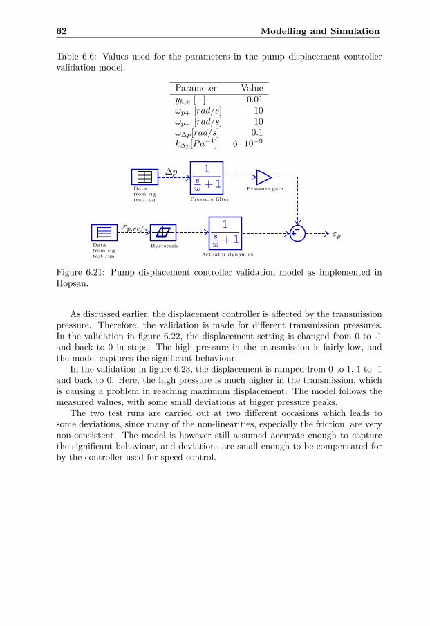
62 Modelling and Simulation
Table 6.6: Values used for the parameters in the pump displacement controllervalidation model.
Parameter Valueyh,p [−] 0.01ωp+ [rad/s] 10ωp− [rad/s] 10ω∆p[rad/s] 0.1k∆p[Pa−1] 6 · 10−9
∆p
Hysteresis
Actuator dynamics
εp,refεp
Pressure filter
Pressure gain
Datafrom rigtest run
Datafrom rigtest run
Figure 6.21: Pump displacement controller validation model as implemented inHopsan.
As discussed earlier, the displacement controller is affected by the transmissionpressure. Therefore, the validation is made for different transmission pressures.In the validation in figure 6.22, the displacement setting is changed from 0 to -1and back to 0 in steps. The high pressure in the transmission is fairly low, andthe model captures the significant behaviour.
In the validation in figure 6.23, the displacement is ramped from 0 to 1, 1 to -1and back to 0. Here, the high pressure is much higher in the transmission, whichis causing a problem in reaching maximum displacement. The model follows themeasured values, with some small deviations at bigger pressure peaks.
The two test runs are carried out at two different occasions which leads tosome deviations, since many of the non-linearities, especially the friction, are verynon-consistent. The model is however still assumed accurate enough to capturethe significant behaviour, and deviations are small enough to be compensated forby the controller used for speed control.
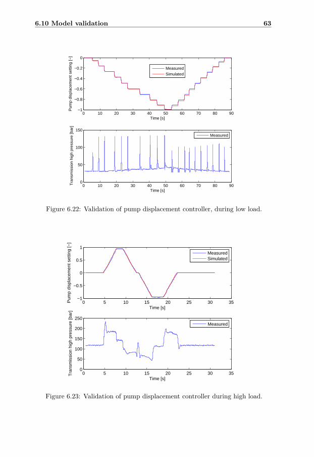
6.10 Model validation 63
0 10 20 30 40 50 60 70 80 90−1
−0.8
−0.6
−0.4
−0.2
0
Time [s]
Pum
p di
spla
cem
ent s
ettin
g [−
]
MeasuredSimulated
0 10 20 30 40 50 60 70 80 900
50
100
150
Time [s]
Tra
nsm
issi
on h
igh
pres
sure
[bar
]
Measured
Figure 6.22: Validation of pump displacement controller, during low load.
0 5 10 15 20 25 30 35−1
−0.5
0
0.5
1
Time [s]
Pum
p di
spla
cem
ent s
ettin
g [−
]
MeasuredSimulated
0 5 10 15 20 25 30 350
50
100
150
200
250
Time [s]
Tra
nsm
issi
on h
igh
pres
sure
[bar
]
Measured
Figure 6.23: Validation of pump displacement controller during high load.
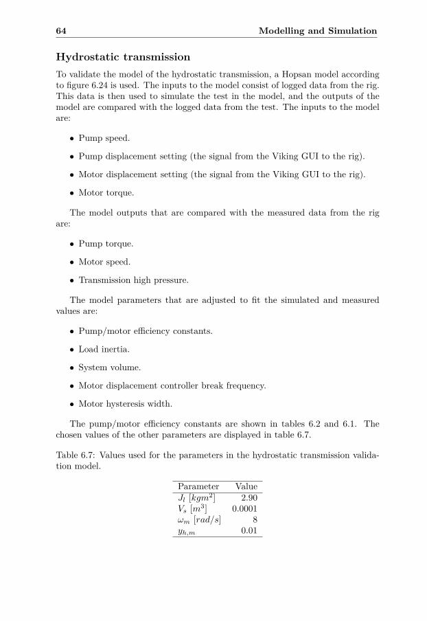
64 Modelling and Simulation
Hydrostatic transmissionTo validate the model of the hydrostatic transmission, a Hopsan model accordingto figure 6.24 is used. The inputs to the model consist of logged data from the rig.This data is then used to simulate the test in the model, and the outputs of themodel are compared with the logged data from the test. The inputs to the modelare:
• Pump speed.
• Pump displacement setting (the signal from the Viking GUI to the rig).
• Motor displacement setting (the signal from the Viking GUI to the rig).
• Motor torque.
The model outputs that are compared with the measured data from the rigare:
• Pump torque.
• Motor speed.
• Transmission high pressure.
The model parameters that are adjusted to fit the simulated and measuredvalues are:
• Pump/motor efficiency constants.
• Load inertia.
• System volume.
• Motor displacement controller break frequency.
• Motor hysteresis width.
The pump/motor efficiency constants are shown in tables 6.2 and 6.1. Thechosen values of the other parameters are displayed in table 6.7.
Table 6.7: Values used for the parameters in the hydrostatic transmission valida-tion model.
Parameter ValueJl [kgm2] 2.90Vs [m3] 0.0001ωm [rad/s] 8yh,m 0.01
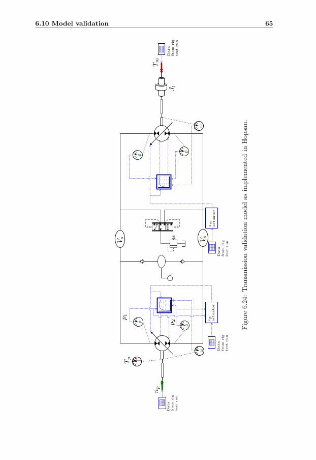
6.10 Model validation 65
εp actuator
εm actuator
Data
from
rig
test
run
Data
from
rig
test
run
TTp
Data
from
rig
test
run
np
p1
p2
Data
from
rig
test
run
Tm
Jl
Vs Vs
Figu
re6.24:Tr
ansm
issionvalid
ationmod
elas
implem
entedin
Hop
san.
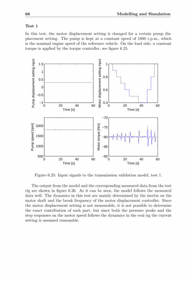
66 Modelling and Simulation
Test 1
In this test, the motor displacement setting is changed for a certain pump dis-placement setting. The pump is kept at a constant speed of 1800 r.p.m., whichis the nominal engine speed of the reference vehicle. On the load side, a constanttorque is applied by the torque controller, see figure 6.25.
0 20 40 60−1
−0.5
0
0.5
1
1.5
Time [s]
Pum
p di
spla
cem
ent s
ettin
g in
put
0 20 40 600.4
0.6
0.8
1
Time [s]
Mot
or d
ispl
acem
ent s
ettin
g in
put
0 20 40 60500
1000
1500
2000
Time [s]
Pum
p sp
eed
[rpm
]
0 20 40 60−90
−85
−80
−75
−70
Time [s]
Mot
or to
rque
[Nm
]
Figure 6.25: Input signals to the transmission validation model, test 1.
The output from the model and the corresponding measured data from the testrig are shown in figure 6.26. As it can be seen, the model follows the measureddata well. The dynamics in this test are mainly determined by the inertia on themotor shaft and the break frequency of the motor displacement controller. Sincethe motor displacement setting is not measurable, it is not possible to determinethe exact contribution of each part, but since both the pressure peaks and thestep responses on the motor speed follows the dynamics in the real rig the currentsetting is assumed reasonable.
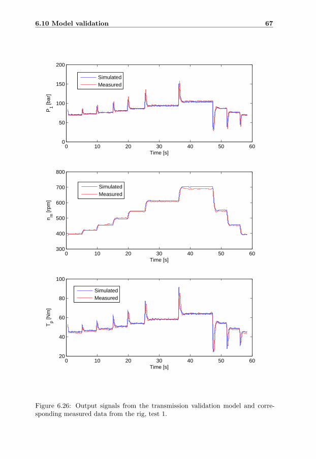
6.10 Model validation 67
0 10 20 30 40 50 600
50
100
150
200
Time [s]
P1 [b
ar]
SimulatedMeasured
0 10 20 30 40 50 60300
400
500
600
700
800
Time [s]
n m [r
pm]
SimulatedMeasured
0 10 20 30 40 50 6020
40
60
80
100
Time [s]
Tp [N
m]
SimulatedMeasured
Figure 6.26: Output signals from the transmission validation model and corre-sponding measured data from the rig, test 1.
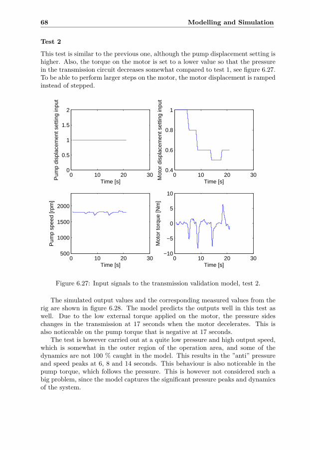
68 Modelling and Simulation
Test 2
This test is similar to the previous one, although the pump displacement setting ishigher. Also, the torque on the motor is set to a lower value so that the pressurein the transmission circuit decreases somewhat compared to test 1, see figure 6.27.To be able to perform larger steps on the motor, the motor displacement is rampedinstead of stepped.
0 10 20 300
0.5
1
1.5
2
Time [s]Pum
p di
spla
cem
ent s
ettin
g in
put
0 10 20 300.4
0.6
0.8
1
Time [s]Mot
or d
ispl
acem
ent s
ettin
g in
put
0 10 20 30500
1000
1500
2000
Time [s]
Pum
p sp
eed
[rpm
]
0 10 20 30−10
−5
0
5
10
Time [s]
Mot
or to
rque
[Nm
]
Figure 6.27: Input signals to the transmission validation model, test 2.
The simulated output values and the corresponding measured values from therig are shown in figure 6.28. The model predicts the outputs well in this test aswell. Due to the low external torque applied on the motor, the pressure sideschanges in the transmission at 17 seconds when the motor decelerates. This isalso noticeable on the pump torque that is negative at 17 seconds.
The test is however carried out at a quite low pressure and high output speed,which is somewhat in the outer region of the operation area, and some of thedynamics are not 100 % caught in the model. This results in the ”anti” pressureand speed peaks at 6, 8 and 14 seconds. This behaviour is also noticeable in thepump torque, which follows the pressure. This is however not considered such abig problem, since the model captures the significant pressure peaks and dynamicsof the system.
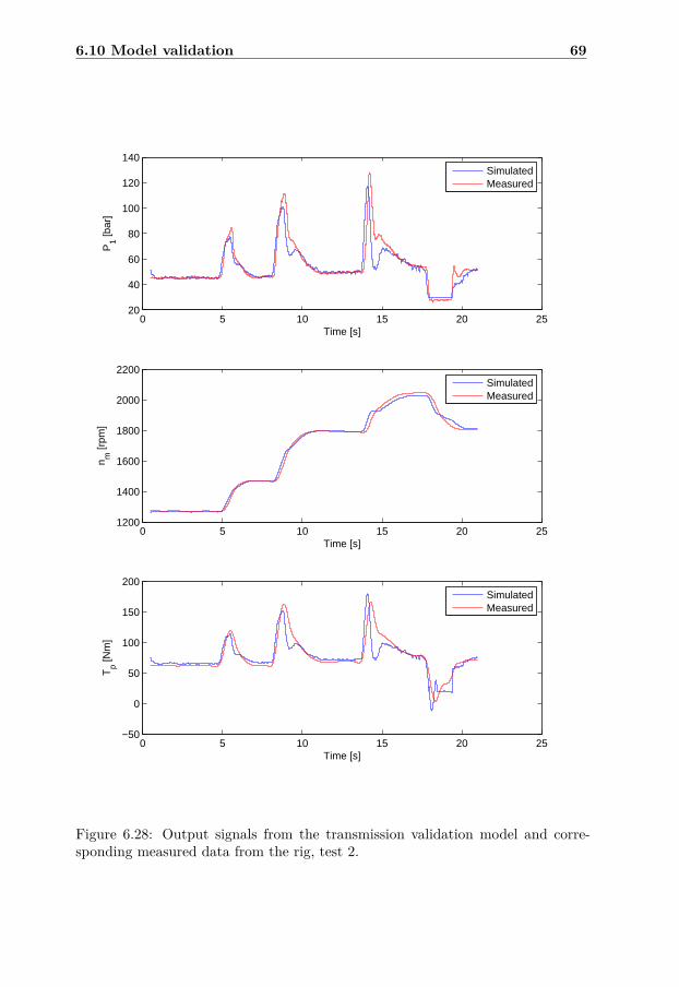
6.10 Model validation 69
0 5 10 15 20 2520
40
60
80
100
120
140
Time [s]
P1 [b
ar]
SimulatedMeasured
0 5 10 15 20 251200
1400
1600
1800
2000
2200
Time [s]
n m [r
pm]
SimulatedMeasured
0 5 10 15 20 25−50
0
50
100
150
200
Time [s]
Tp [N
m]
SimulatedMeasured
Figure 6.28: Output signals from the transmission validation model and corre-sponding measured data from the rig, test 2.
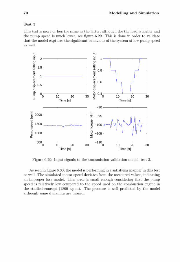
70 Modelling and Simulation
Test 3
This test is more or less the same as the latter, although the the load is higher andthe pump speed is much lower, see figure 6.29. This is done in order to validatethat the model captures the significant behaviour of the system at low pump speedas well.
0 10 20 300
0.5
1
1.5
2
Time [s]Pum
p di
spla
cem
ent s
ettin
g in
put
0 10 20 300.4
0.6
0.8
1
Time [s]Mot
or d
ispl
acem
ent s
ettin
g in
put
0 10 20 30500
1000
1500
2000
Time [s]
Pum
p sp
eed
[rpm
]
0 10 20 30−110
−105
−100
−95
−90
Time [s]
Mot
or to
rque
[Nm
]
Figure 6.29: Input signals to the transmission validation model, test 3.
As seen in figure 6.30, the model is performing in a satisfying manner in this testas well. The simulated motor speed deviates from the measured values, indicatingan improper loss model. This error is small enough considering that the pumpspeed is relatively low compared to the speed used on the combustion engine inthe studied concept (1800 r.p.m). The pressure is well predicted by the modelalthough some dynamics are missed.
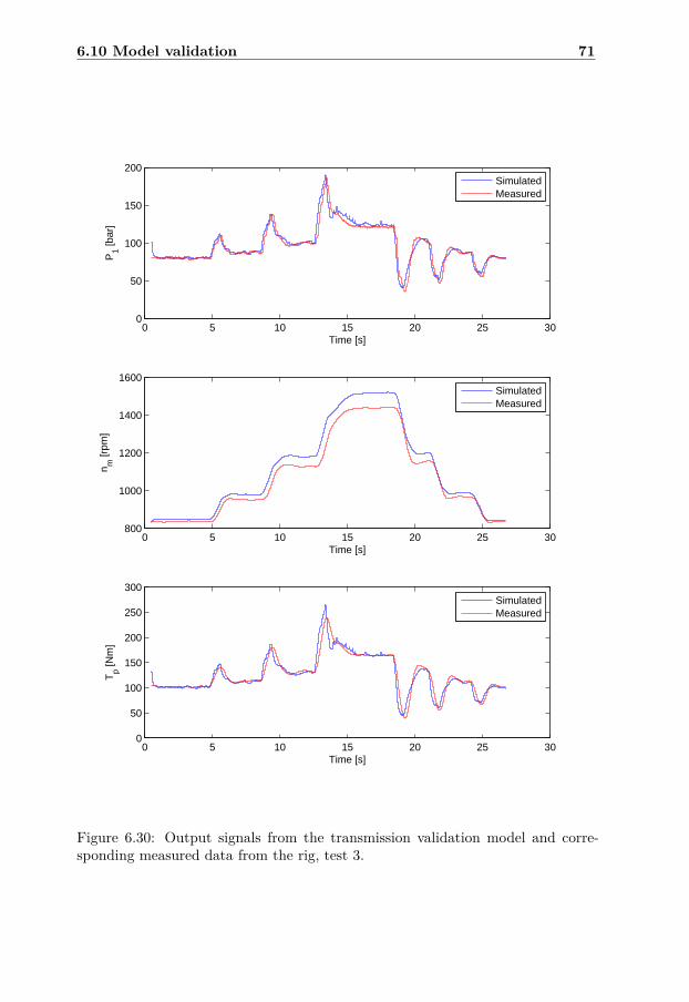
6.10 Model validation 71
0 5 10 15 20 25 300
50
100
150
200
Time [s]
P1 [b
ar]
SimulatedMeasured
0 5 10 15 20 25 30800
1000
1200
1400
1600
Time [s]
n m [r
pm]
SimulatedMeasured
0 5 10 15 20 25 300
50
100
150
200
250
300
Time [s]
Tp [N
m]
SimulatedMeasured
Figure 6.30: Output signals from the transmission validation model and corre-sponding measured data from the rig, test 3.
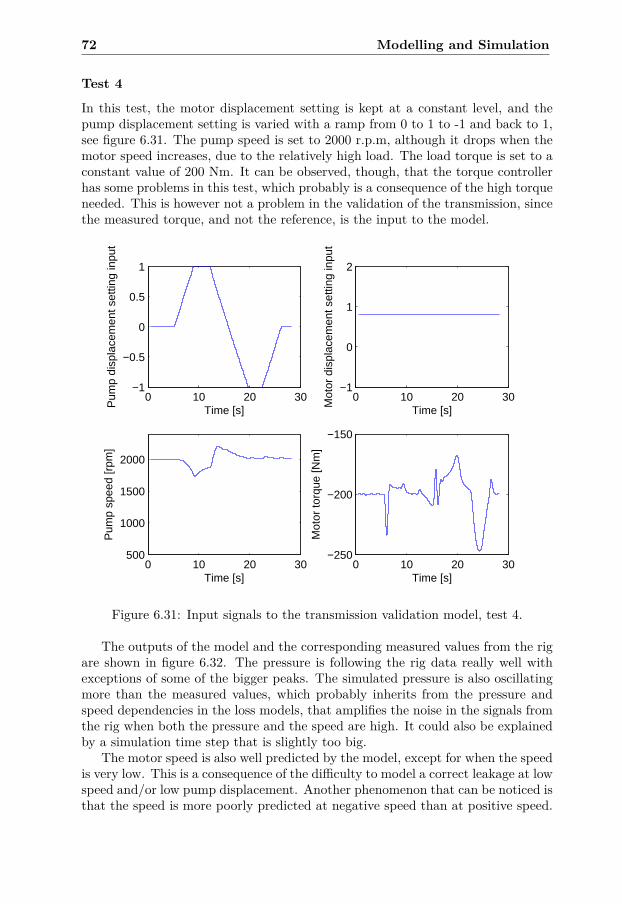
72 Modelling and Simulation
Test 4
In this test, the motor displacement setting is kept at a constant level, and thepump displacement setting is varied with a ramp from 0 to 1 to -1 and back to 1,see figure 6.31. The pump speed is set to 2000 r.p.m, although it drops when themotor speed increases, due to the relatively high load. The load torque is set to aconstant value of 200 Nm. It can be observed, though, that the torque controllerhas some problems in this test, which probably is a consequence of the high torqueneeded. This is however not a problem in the validation of the transmission, sincethe measured torque, and not the reference, is the input to the model.
0 10 20 30−1
−0.5
0
0.5
1
Time [s]Pum
p di
spla
cem
ent s
ettin
g in
put
0 10 20 30−1
0
1
2
Time [s]Mot
or d
ispl
acem
ent s
ettin
g in
put
0 10 20 30500
1000
1500
2000
Time [s]
Pum
p sp
eed
[rpm
]
0 10 20 30−250
−200
−150
Time [s]
Mot
or to
rque
[Nm
]
Figure 6.31: Input signals to the transmission validation model, test 4.
The outputs of the model and the corresponding measured values from the rigare shown in figure 6.32. The pressure is following the rig data really well withexceptions of some of the bigger peaks. The simulated pressure is also oscillatingmore than the measured values, which probably inherits from the pressure andspeed dependencies in the loss models, that amplifies the noise in the signals fromthe rig when both the pressure and the speed are high. It could also be explainedby a simulation time step that is slightly too big.
The motor speed is also well predicted by the model, except for when the speedis very low. This is a consequence of the difficulty to model a correct leakage at lowspeed and/or low pump displacement. Another phenomenon that can be noticed isthat the speed is more poorly predicted at negative speed than at positive speed.
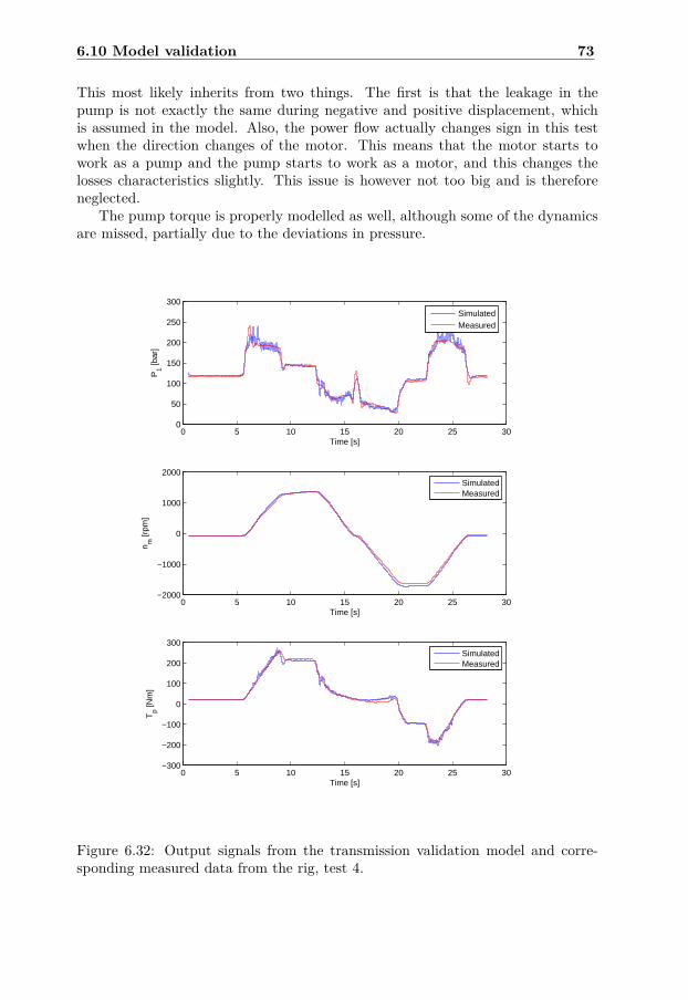
6.10 Model validation 73
This most likely inherits from two things. The first is that the leakage in thepump is not exactly the same during negative and positive displacement, whichis assumed in the model. Also, the power flow actually changes sign in this testwhen the direction changes of the motor. This means that the motor starts towork as a pump and the pump starts to work as a motor, and this changes thelosses characteristics slightly. This issue is however not too big and is thereforeneglected.
The pump torque is properly modelled as well, although some of the dynamicsare missed, partially due to the deviations in pressure.
0 5 10 15 20 25 300
50
100
150
200
250
300
Time [s]
P1 [b
ar]
SimulatedMeasured
0 5 10 15 20 25 30−2000
−1000
0
1000
2000
Time [s]
n m [r
pm]
SimulatedMeasured
0 5 10 15 20 25 30−300
−200
−100
0
100
200
300
Time [s]
Tp [N
m]
SimulatedMeasured
Figure 6.32: Output signals from the transmission validation model and corre-sponding measured data from the rig, test 4.
74 Modelling and Simulation
Minor conclusion
To summarise, the developed model captures the significant behaviour of the sys-tem. Although the results deviates in certain operation points, the errors are notextreme which implies that the model is accurate enough in the considered oper-ating area. An important factor to consider here is also that the aim of the modelis to control it, which means that deviations are tolerable to some extent since thecontroller will handle the error.
6.11 Linear hydrostatic transmission modelThe previously derived and validated model of the hydrostatic transmission isstrictly non-linear and is used in the Hopsan simulations. In order to furtheranalyse the system, and draw more conclusions about it, a simple linear model ofthe hydrostatic transmission is derived as well.
The input signal to the transmission is considered as the displacement settingratio iε which is related to the hydrostatic transmission speed ratio (chapter 2,equation (2.4)):
iε = εp
εm∝ ih (6.21)
The transfer function of the transmission from transmission displacement ratioiε to motor speed nm linearised at a certain motor displacement setting εm,0 canthen be expressed as [3]:
∆nm =Dpnp
Dm
s2
ω2h
+ 2δhs
ωh+ 1
∆iε (6.22)
where the hydraulic eigenfrequency ωh and the hydraulic damping δh is
ωh =
√βe (Dmεm,0)2
V0Jeqand δh = Ct
2Dmεm,0
√βeJeq
V0+ Bm
2Dmεm,0
√V0
βeJeq(6.23)
If the dynamics of the displacement controller is included as well the totaltransfer function yields:
∆nm =
Dpnp
Dm·(
11+ s
wp/m
)s2
ω2h
+ 2δhs
ωh+ 1
∆iε (6.24)
The actuator break frequency wp/m changes depending on whether the pumpor the motor is currently controlled, but in order to investigate the worst casescenario (from a stability perspective) the value of the motor actuator is usedsince the motor actuator has the lowest break frequency.
The numerical values for the linear model are shown in table 6.8. For theparameters that are constant, the same values as in the Hopsan model is used. Forthe leakage coefficient and the viscous friction, average values from the Hopsan
6.11 Linear hydrostatic transmission model 75
model are used. Since the controlled variable is the vehicle speed, the viscousfriction should actually be slightly higher than the value for the viscous friction inthe hydrostatic transmission. Here, this matter is neglected since the fundamentalbehaviour of the transmission still will be captured in the model.
Table 6.8: Values used for the parameters in the linear model of the hydrostatictransmission. The values for the inertia are displayed in table 6.9.
Parameter ValueDm 152.1 cm3/revDp 110.4 cm3/revnp 1800 r.p.m.βe 1000 MPaV0 0.0001 m3
Bm 1.5 Nms/radCt 3.1 · 10−11 m5/Nswm/p 8 rad/s
The inertia as experienced by the motor is referred to as the equivalent inertia,and depends on the vehicle mass and the transmission gear ratio. The equivalentinertia in the studied concept varies depending on the current mode according to:
Jeq =
mveh · (rwi0iH)2 in hydrostatic mode
mveh ·(
rwi0iS
1− 1R
)2in power-split mode
(6.25)
The numerical values for equivalent inertias are shown in table 6.9.
Table 6.9: Equivalent motor inertias for studied transmission concept at a modeshift speed of 7 km/h
Hydrostatic mode Power-split modeJeq [kgm2] 0.75 4.17
The bode diagrams for the transfer function in (6.24) with the numerical valuesin tables 6.8 and 6.9 are shown in figure 6.33. The system is linearised in εm,0 = 1.The negative amplitude and phase margins suggest a low gain in order to reacha stable control. It can also be seen that the break frequency of the actuator dy-namics is lower than the resonance frequency of the transmission. This affects thestability margins, as the phase crosses -180 degrees at a relatively low frequency.In other words, the slow machine control units limit the control of the system.
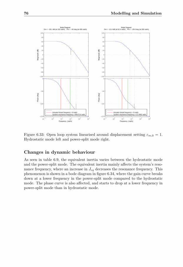
76 Modelling and Simulation
−100
−80
−60
−40
−20
0
20
40
60
80
100
Mag
nitu
de (
dB)
10−1
100
101
102
103
104
−270
−180
−90
0
Pha
se (
deg)
Bode DiagramGm = −28.1 dB (at 102 rad/s) , Pm = −50 deg (at 406 rad/s)
Frequency (rad/s)
Actuator break frequency = 8 rad/sSystem resonance frequency = 88.6714 rad/s
−100
−80
−60
−40
−20
0
20
40
60
80
100
Mag
nitu
de (
dB)
10−1
100
101
102
103
104
−270
−180
−90
0
Pha
se (
deg)
Bode DiagramGm = −21.6 dB (at 62.4 rad/s) , Pm = −29.6 deg (at 200 rad/s)
Frequency (rad/s)
Actuator break frequency = 8 rad/sSystem resonance frequency = 37.4992 rad/s
Figure 6.33: Open loop system linearised around displacement setting εm,0 = 1.Hydrostatic mode left and power-split mode right.
Changes in dynamic behaviourAs seen in table 6.9, the equivalent inertia varies between the hydrostatic modeand the power-split mode. The equivalent inertia mainly affects the system’s reso-nance frequency, where an increase in Jeq decreases the resonance frequency. Thisphenomenon is shown in a bode diagram in figure 6.34, where the gain curve breaksdown at a lower frequency in the power-split mode compared to the hydrostaticmode. The phase curve is also affected, and starts to drop at a lower frequency inpower-split mode than in hydrostatic mode.
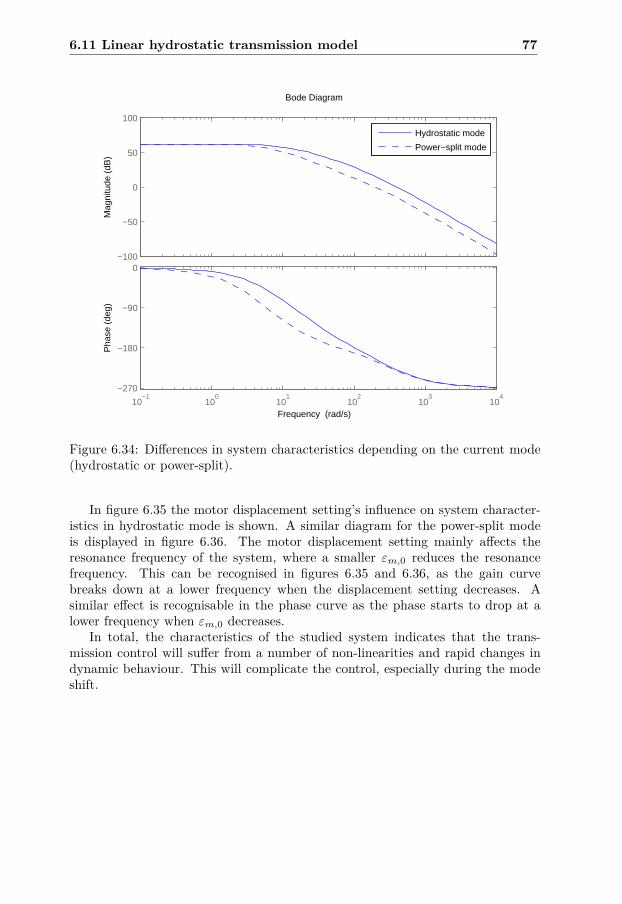
6.11 Linear hydrostatic transmission model 77
−100
−50
0
50
100M
agni
tude
(dB
)
10−1
100
101
102
103
104
−270
−180
−90
0
Pha
se (
deg)
Bode Diagram
Frequency (rad/s)
Hydrostatic mode
Power−split mode
Figure 6.34: Differences in system characteristics depending on the current mode(hydrostatic or power-split).
In figure 6.35 the motor displacement setting’s influence on system character-istics in hydrostatic mode is shown. A similar diagram for the power-split modeis displayed in figure 6.36. The motor displacement setting mainly affects theresonance frequency of the system, where a smaller εm,0 reduces the resonancefrequency. This can be recognised in figures 6.35 and 6.36, as the gain curvebreaks down at a lower frequency when the displacement setting decreases. Asimilar effect is recognisable in the phase curve as the phase starts to drop at alower frequency when εm,0 decreases.
In total, the characteristics of the studied system indicates that the trans-mission control will suffer from a number of non-linearities and rapid changes indynamic behaviour. This will complicate the control, especially during the modeshift.
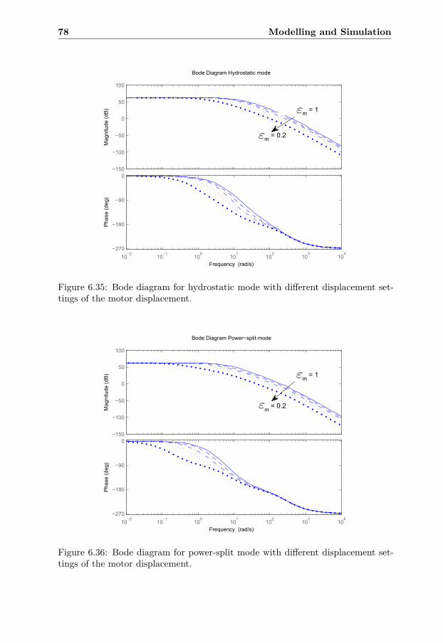
78 Modelling and Simulation
−150
−100
−50
0
50
100
Mag
nitu
der(
dB)
10−2
10−1
100
101
102
103
104
−270
−180
−90
0
Pha
ser(
deg)
epsm
=r1
epsm
=r0.2
BoderDiagramrHydrostaticrmode
Frequencyr (rad/s)
Figure 6.35: Bode diagram for hydrostatic mode with different displacement set-tings of the motor displacement.
−150
−100
−50
0
50
100
Mag
nitu
der(
dB)
10−2
10−1
100
101
102
103
104
−270
−180
−90
0
Pha
ser(
deg)
epsm
=r1
epsm
=r0.2
BoderDiagramrPower−splitrmode
Frequencyr (rad/s)
Figure 6.36: Bode diagram for power-split mode with different displacement set-tings of the motor displacement.
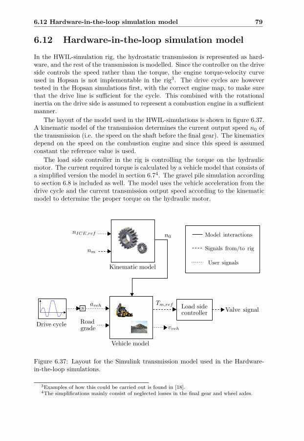
6.12 Hardware-in-the-loop simulation model 79
6.12 Hardware-in-the-loop simulation model
In the HWIL-simulation rig, the hydrostatic transmission is represented as hard-ware, and the rest of the transmission is modelled. Since the controller on the driveside controls the speed rather than the torque, the engine torque-velocity curveused in Hopsan is not implementable in the rig3. The drive cycles are howevertested in the Hopsan simulations first, with the correct engine map, to make surethat the drive line is sufficient for the cycle. This combined with the rotationalinertia on the drive side is assumed to represent a combustion engine in a sufficientmanner.
The layout of the model used in the HWIL-simulations is shown in figure 6.37.A kinematic model of the transmission determines the current output speed n0 ofthe transmission (i.e. the speed on the shaft before the final gear). The kinematicsdepend on the speed on the combustion engine and since this speed is assumedconstant the reference value is used.
The load side controller in the rig is controlling the torque on the hydraulicmotor. The current required torque is calculated by a vehicle model that consists ofa simplified version the model in section 6.74. The gravel pile simulation accordingto section 6.8 is included as well. The model uses the vehicle acceleration from thedrive cycle and the current transmission output speed according to the kinematicmodel to determine the proper torque on the hydraulic motor.
Figure 6.37: Layout for the Simulink transmission model used in the Hardware-in-the-loop simulations.
3Examples of how this could be carried out is found in [18].4The simplifications mainly consist of neglected losses in the final gear and wheel axles.
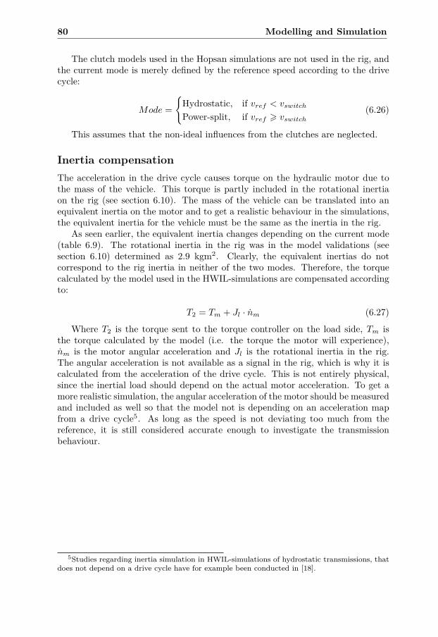
80 Modelling and Simulation
The clutch models used in the Hopsan simulations are not used in the rig, andthe current mode is merely defined by the reference speed according to the drivecycle:
Mode ={Hydrostatic, if vref < vswitch
Power-split, if vref > vswitch
(6.26)
This assumes that the non-ideal influences from the clutches are neglected.
Inertia compensationThe acceleration in the drive cycle causes torque on the hydraulic motor due tothe mass of the vehicle. This torque is partly included in the rotational inertiaon the rig (see section 6.10). The mass of the vehicle can be translated into anequivalent inertia on the motor and to get a realistic behaviour in the simulations,the equivalent inertia for the vehicle must be the same as the inertia in the rig.
As seen earlier, the equivalent inertia changes depending on the current mode(table 6.9). The rotational inertia in the rig was in the model validations (seesection 6.10) determined as 2.9 kgm2. Clearly, the equivalent inertias do notcorrespond to the rig inertia in neither of the two modes. Therefore, the torquecalculated by the model used in the HWIL-simulations are compensated accordingto:
T2 = Tm + Jl · nm (6.27)
Where T2 is the torque sent to the torque controller on the load side, Tm isthe torque calculated by the model (i.e. the torque the motor will experience),nm is the motor angular acceleration and Jl is the rotational inertia in the rig.The angular acceleration is not available as a signal in the rig, which is why it iscalculated from the acceleration of the drive cycle. This is not entirely physical,since the inertial load should depend on the actual motor acceleration. To get amore realistic simulation, the angular acceleration of the motor should be measuredand included as well so that the model not is depending on an acceleration mapfrom a drive cycle5. As long as the speed is not deviating too much from thereference, it is still considered accurate enough to investigate the transmissionbehaviour.
5Studies regarding inertia simulation in HWIL-simulations of hydrostatic transmissions, thatdoes not depend on a drive cycle have for example been conducted in [18].
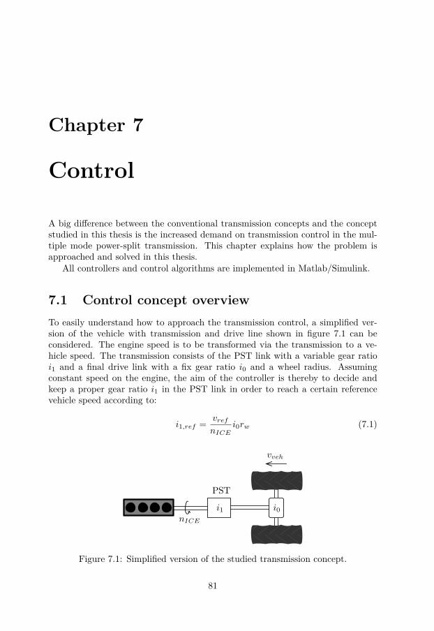
Chapter 7
Control
A big difference between the conventional transmission concepts and the conceptstudied in this thesis is the increased demand on transmission control in the mul-tiple mode power-split transmission. This chapter explains how the problem isapproached and solved in this thesis.
All controllers and control algorithms are implemented in Matlab/Simulink.
7.1 Control concept overviewTo easily understand how to approach the transmission control, a simplified ver-sion of the vehicle with transmission and drive line shown in figure 7.1 can beconsidered. The engine speed is to be transformed via the transmission to a ve-hicle speed. The transmission consists of the PST link with a variable gear ratioi1 and a final drive link with a fix gear ratio i0 and a wheel radius. Assumingconstant speed on the engine, the aim of the controller is thereby to decide andkeep a proper gear ratio i1 in the PST link in order to reach a certain referencevehicle speed according to:
i1,ref = vref
nICEi0rw (7.1)
i0i1
vveh
nICE
PST
Figure 7.1: Simplified version of the studied transmission concept.
81
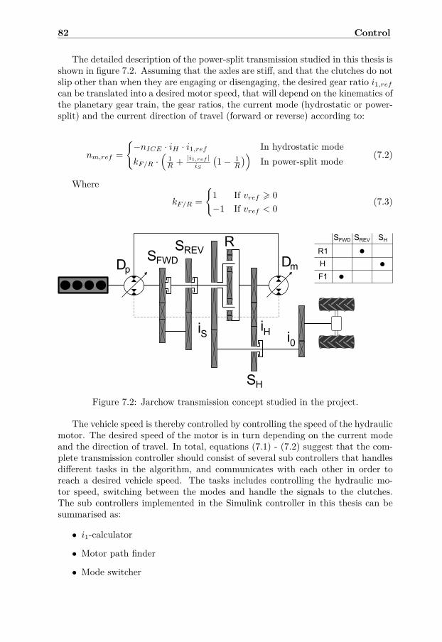
82 Control
The detailed description of the power-split transmission studied in this thesis isshown in figure 7.2. Assuming that the axles are stiff, and that the clutches do notslip other than when they are engaging or disengaging, the desired gear ratio i1,ref
can be translated into a desired motor speed, that will depend on the kinematics ofthe planetary gear train, the gear ratios, the current mode (hydrostatic or power-split) and the current direction of travel (forward or reverse) according to:
nm,ref ={−nICE · iH · i1,ref In hydrostatic modekF/R ·
(1R + |i1,ref |
iS
(1− 1
R
))In power-split mode
(7.2)
Where
kF/R ={
1 If vref > 0−1 If vref < 0
(7.3)
Figure 7.2: Jarchow transmission concept studied in the project.
The vehicle speed is thereby controlled by controlling the speed of the hydraulicmotor. The desired speed of the motor is in turn depending on the current modeand the direction of travel. In total, equations (7.1) - (7.2) suggest that the com-plete transmission controller should consist of several sub controllers that handlesdifferent tasks in the algorithm, and communicates with each other in order toreach a desired vehicle speed. The tasks includes controlling the hydraulic mo-tor speed, switching between the modes and handle the signals to the clutches.The sub controllers implemented in the Simulink controller in this thesis can besummarised as:
• i1-calculator
• Motor path finder
• Mode switcher
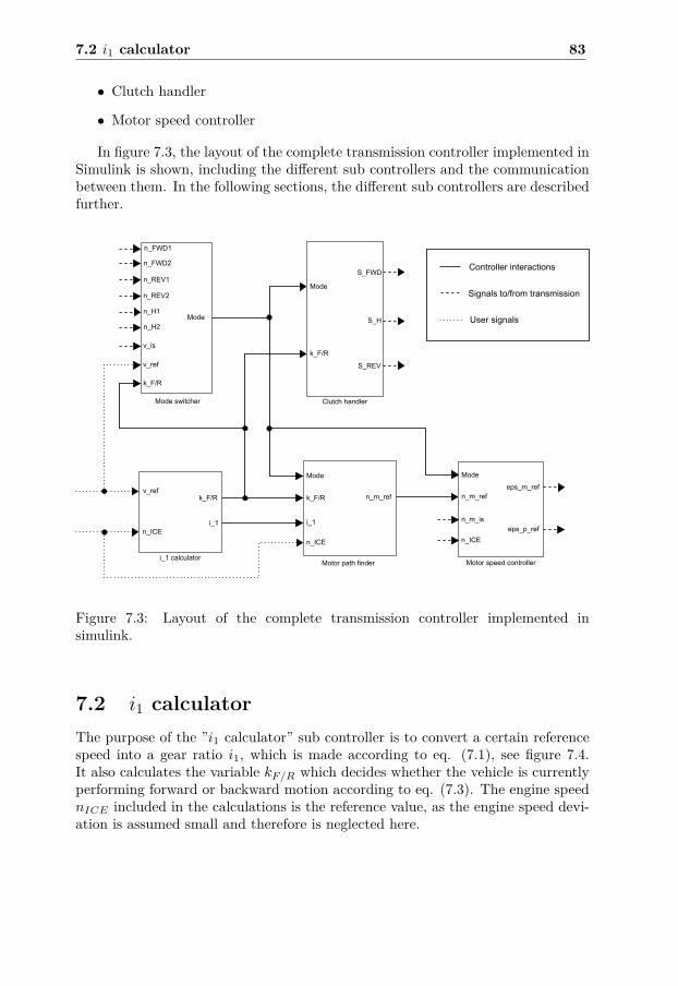
7.2 i1 calculator 83
• Clutch handler
• Motor speed controller
In figure 7.3, the layout of the complete transmission controller implemented inSimulink is shown, including the different sub controllers and the communicationbetween them. In the following sections, the different sub controllers are describedfurther.
Figure 7.3: Layout of the complete transmission controller implemented insimulink.
7.2 i1 calculatorThe purpose of the ”i1 calculator” sub controller is to convert a certain referencespeed into a gear ratio i1, which is made according to eq. (7.1), see figure 7.4.It also calculates the variable kF/R which decides whether the vehicle is currentlyperforming forward or backward motion according to eq. (7.3). The engine speednICE included in the calculations is the reference value, as the engine speed devi-ation is assumed small and therefore is neglected here.
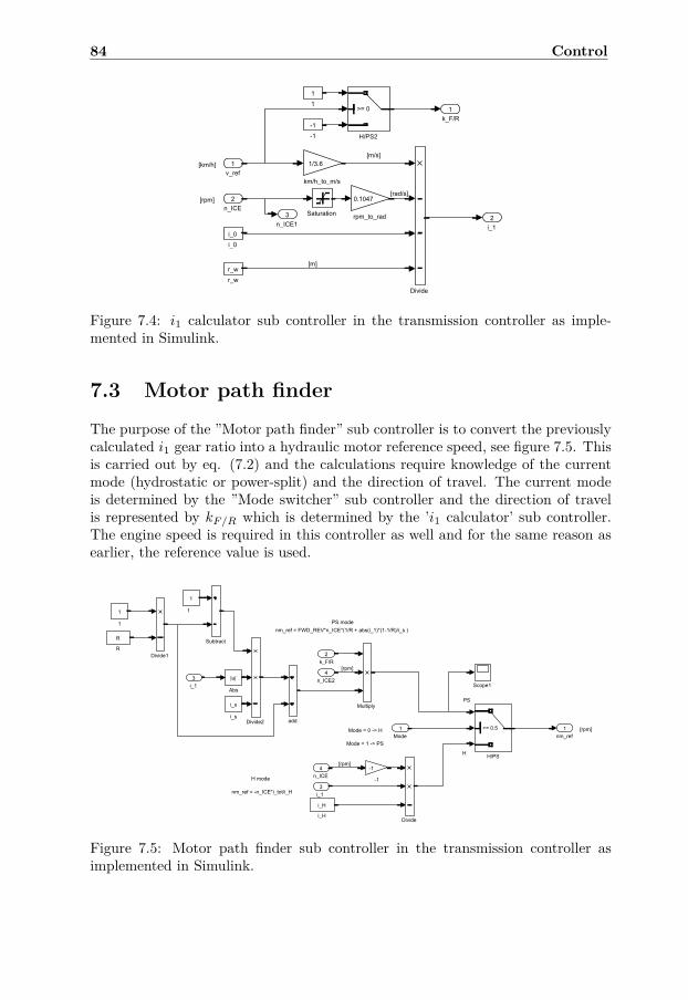
84 Control
Figure 7.4: i1 calculator sub controller in the transmission controller as imple-mented in Simulink.
7.3 Motor path finder
The purpose of the ”Motor path finder” sub controller is to convert the previouslycalculated i1 gear ratio into a hydraulic motor reference speed, see figure 7.5. Thisis carried out by eq. (7.2) and the calculations require knowledge of the currentmode (hydrostatic or power-split) and the direction of travel. The current modeis determined by the ”Mode switcher” sub controller and the direction of travelis represented by kF/R which is determined by the ’i1 calculator’ sub controller.The engine speed is required in this controller as well and for the same reason asearlier, the reference value is used.
Figure 7.5: Motor path finder sub controller in the transmission controller asimplemented in Simulink.
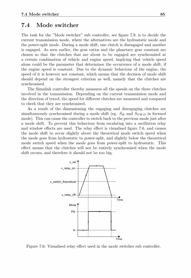
7.4 Mode switcher 85
7.4 Mode switcherThe task for the ”Mode switcher” sub controller, see figure 7.9, is to decide thecurrent transmission mode, where the alternatives are the hydrostatic mode andthe power-split mode. During a mode shift, one clutch is disengaged and anotheris engaged. As seen earlier, the gear ratios and the planetary gear constant arechosen so that the clutches that are about to be engaged are synchronised ata certain combination of vehicle and engine speed, implying that vehicle speedalone could be the parameter that determines the occurrence of a mode shift, ifthe engine speed is constant. Due to the dynamic behaviour of the engine, thespeed of it is however not constant, which means that the decision of mode shiftshould depend on the strongest criterion as well, namely that the clutches aresynchronised.
The Simulink controller thereby measures all the speeds on the three clutchesinvolved in the transmission. Depending on the current transmission mode andthe direction of travel, the speed for different clutches are measured and comparedto check that they are synchronised.
As a result of the dimensioning the engaging and disengaging clutches aresimultaneously synchronised during a mode shift (eg. SH and SF W D in forwardmode). This can cause the controller to switch back to the previous mode just aftera mode shift. To prevent this behaviour from escalating into a oscillation relayand window effects are used. The relay effect is visualised figure 7.6, and causesthe mode shift to occur slightly above the theoretical mode switch speed whenthe mode goes from hydrostatic to power-split, and slightly below the theoreticalmode switch speed when the mode goes from power-split to hydrostatic. Thiseffect means that the clutches will not be entirely synchronised when the modeshift occurs, and therefore it should not be too big.
Figure 7.6: Visualised relay effect used in the mode switcher sub controller.
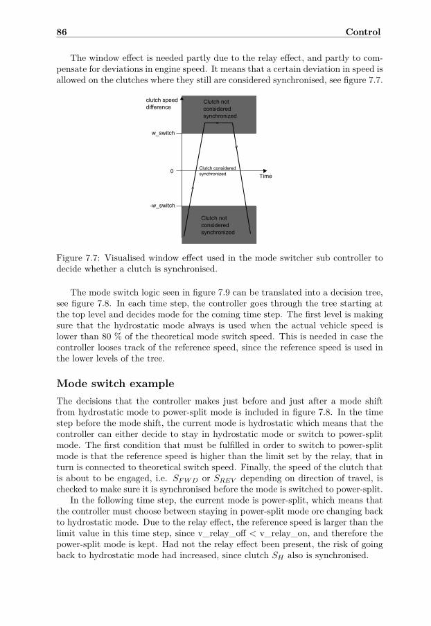
86 Control
The window effect is needed partly due to the relay effect, and partly to com-pensate for deviations in engine speed. It means that a certain deviation in speed isallowed on the clutches where they still are considered synchronised, see figure 7.7.
Figure 7.7: Visualised window effect used in the mode switcher sub controller todecide whether a clutch is synchronised.
The mode switch logic seen in figure 7.9 can be translated into a decision tree,see figure 7.8. In each time step, the controller goes through the tree starting atthe top level and decides mode for the coming time step. The first level is makingsure that the hydrostatic mode always is used when the actual vehicle speed islower than 80 % of the theoretical mode switch speed. This is needed in case thecontroller looses track of the reference speed, since the reference speed is used inthe lower levels of the tree.
Mode switch exampleThe decisions that the controller makes just before and just after a mode shiftfrom hydrostatic mode to power-split mode is included in figure 7.8. In the timestep before the mode shift, the current mode is hydrostatic which means that thecontroller can either decide to stay in hydrostatic mode or switch to power-splitmode. The first condition that must be fulfilled in order to switch to power-splitmode is that the reference speed is higher than the limit set by the relay, that inturn is connected to theoretical switch speed. Finally, the speed of the clutch thatis about to be engaged, i.e. SF W D or SREV depending on direction of travel, ischecked to make sure it is synchronised before the mode is switched to power-split.
In the following time step, the current mode is power-split, which means thatthe controller must choose between staying in power-split mode ore changing backto hydrostatic mode. Due to the relay effect, the reference speed is larger than thelimit value in this time step, since v_relay_off < v_relay_on, and therefore thepower-split mode is kept. Had not the relay effect been present, the risk of goingback to hydrostatic mode had increased, since clutch SH also is synchronised.
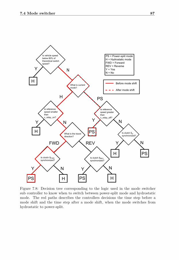
7.4 Mode switcher 87
Figure 7.8: Decision tree corresponding to the logic used in the mode switchersub controller to know when to switch between power-split mode and hydrostaticmode. The red paths describes the controllers decisions the time step before amode shift and the time step after a mode shift, when the mode switches fromhydrostatic to power-split.
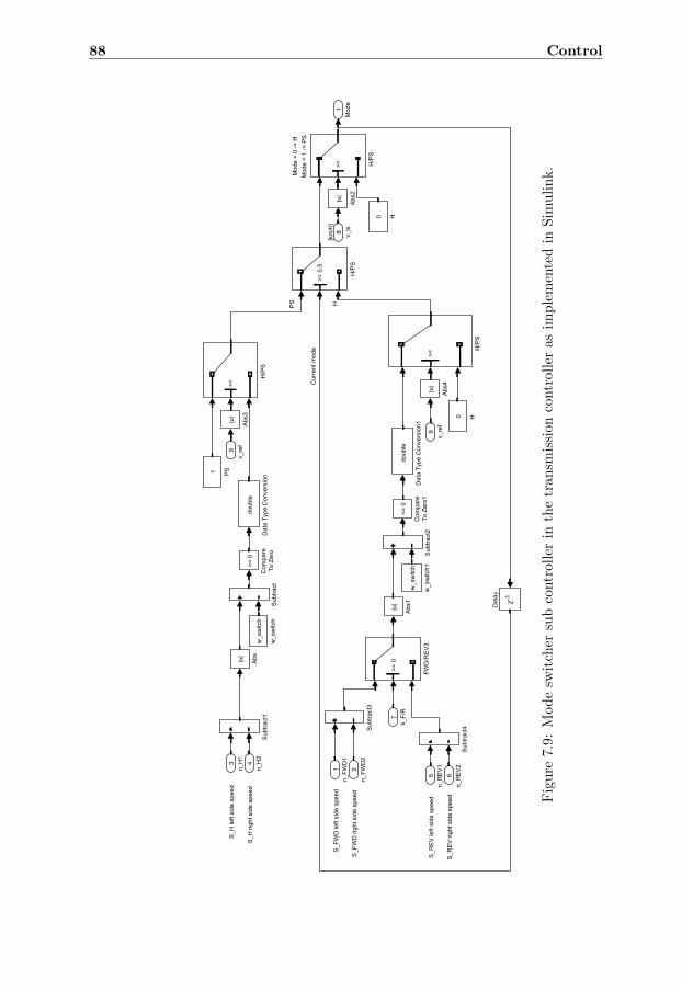
88 Control
Figu
re7.9:
Mod
esw
itche
rsubcontrolle
rin
thetran
smiss
ioncontrolle
ras
implem
entedin
Simulink.
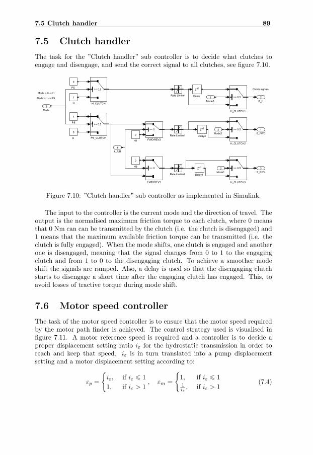
7.5 Clutch handler 89
7.5 Clutch handlerThe task for the ”Clutch handler” sub controller is to decide what clutches toengage and disengage, and send the correct signal to all clutches, see figure 7.10.
Figure 7.10: ”Clutch handler” sub controller as implemented in Simulink.
The input to the controller is the current mode and the direction of travel. Theoutput is the normalised maximum friction torque to each clutch, where 0 meansthat 0 Nm can can be transmitted by the clutch (i.e. the clutch is disengaged) and1 means that the maximum available friction torque can be transmitted (i.e. theclutch is fully engaged). When the mode shifts, one clutch is engaged and anotherone is disengaged, meaning that the signal changes from 0 to 1 to the engagingclutch and from 1 to 0 to the disengaging clutch. To achieve a smoother modeshift the signals are ramped. Also, a delay is used so that the disengaging clutchstarts to disengage a short time after the engaging clutch has engaged. This, toavoid losses of tractive torque during mode shift.
7.6 Motor speed controllerThe task of the motor speed controller is to ensure that the motor speed requiredby the motor path finder is achieved. The control strategy used is visualised infigure 7.11. A motor reference speed is required and a controller is to decide aproper displacement setting ratio iε for the hydrostatic transmission in order toreach and keep that speed. iε is in turn translated into a pump displacementsetting and a motor displacement setting according to:
εp ={iε, if iε 6 11, if iε > 1
, εm ={
1, if iε 6 11iε, if iε > 1
(7.4)
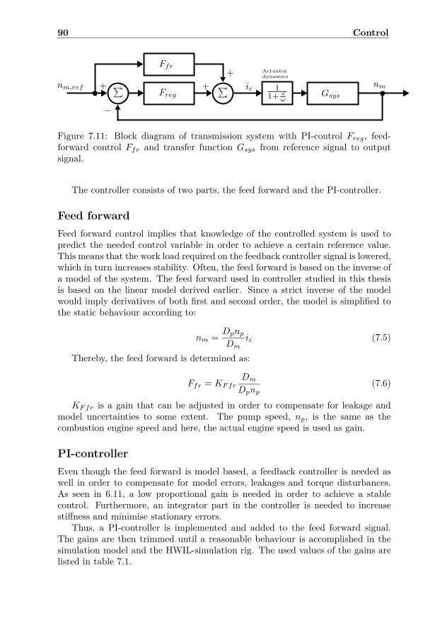
90 Control
Ffr
Freg
∑ ∑ iεnm,ref
−
+Actuatordynamics
Gsys
nm
++
Figure 7.11: Block diagram of transmission system with PI-control Freg, feed-forward control Ffr and transfer function Gsys from reference signal to outputsignal.
The controller consists of two parts, the feed forward and the PI-controller.
Feed forwardFeed forward control implies that knowledge of the controlled system is used topredict the needed control variable in order to achieve a certain reference value.This means that the work load required on the feedback controller signal is lowered,which in turn increases stability. Often, the feed forward is based on the inverse ofa model of the system. The feed forward used in controller studied in this thesisis based on the linear model derived earlier. Since a strict inverse of the modelwould imply derivatives of both first and second order, the model is simplified tothe static behaviour according to:
nm = Dpnp
Dmiε (7.5)
Thereby, the feed forward is determined as:
Ffr = KF frDm
Dpnp(7.6)
KF fr is a gain that can be adjusted in order to compensate for leakage andmodel uncertainties to some extent. The pump speed, np, is the same as thecombustion engine speed and here, the actual engine speed is used as gain.
PI-controllerEven though the feed forward is model based, a feedback controller is needed aswell in order to compensate for model errors, leakages and torque disturbances.As seen in 6.11, a low proportional gain is needed in order to achieve a stablecontrol. Furthermore, an integrator part in the controller is needed to increasestiffness and minimise stationary errors.
Thus, a PI-controller is implemented and added to the feed forward signal.The gains are then trimmed until a reasonable behaviour is accomplished in thesimulation model and the HWIL-simulation rig. The used values of the gains arelisted in table 7.1.
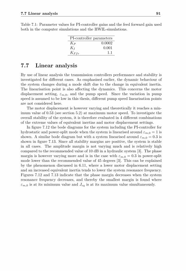
7.7 Linear analysis 91
Table 7.1: Parameter values for PI-controller gains and the feed forward gain usedboth in the computer simulations and the HWIL-simulations.
PI-controller parametersKP 0.0002KI 0.001KF fr 1.1
7.7 Linear analysisBy use of linear analysis the transmission controllers performance and stability isinvestigated for different cases. As emphasised earlier, the dynamic behaviour ofthe system changes during a mode shift due to the change in equivalent inertia.The linearisation point is also affecting the dynamics. This concerns the motordisplacement setting, εm,0, and the pump speed. Since the variation in pumpspeed is assumed to be low in this thesis, different pump speed linearisation pointsare not considered here.
The motor displacement is however varying and theoretically it reaches a min-imum value of 0.53 (see section 5.2) at maximum motor speed. To investigate theoverall stability of the system, it is therefore evaluated in 4 different combinationsof the extreme values of equivalent inertias and motor displacement settings.
In figure 7.12 the bode diagrams for the system including the PI-controller forhydrostatic and power-split mode when the system is linearised around εm,0 = 1 isshown. A similar bode diagram but with a system linearised around εm,0 = 0.3 isshown in figure 7.13. Since all stability margins are positive, the system is stablein all cases. The amplitude margin is not varying much and is relatively highcompared to the recommended value of 10 dB in a hydraulic system [3]. The phasemargin is however varying more and is in the case with εm,0 = 0.3 in power-splitmode lower than the recommended value of 45 degrees [3]. This can be explainedby the phenomenon discussed in 6.11, where a lower motor displacement settingand an increased equivalent inertia tends to lower the system resonance frequency.Figures 7.12 and 7.13 indicate that the phase margin decreases when the systemresonance frequency decreases, and thereby the smallest margin is found whereεm,0 is at its minimum value and Jeq is at its maximum value simultaneously.
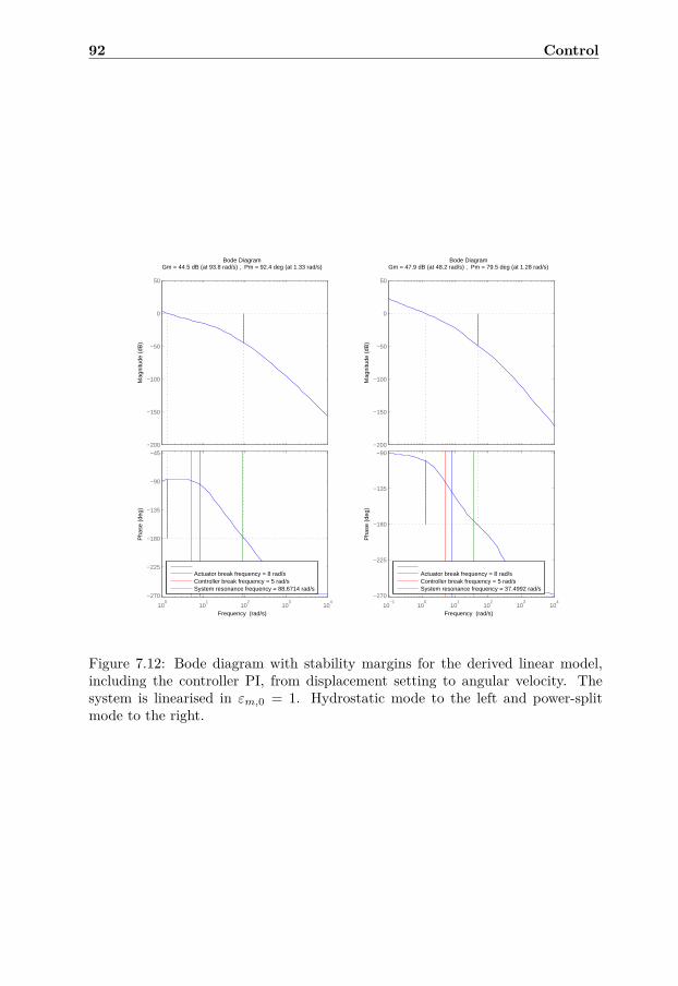
92 Control
−200
−150
−100
−50
0
50
Mag
nitu
de (
dB)
100
101
102
103
104
−270
−225
−180
−135
−90
−45
Pha
se (
deg)
Bode DiagramGm = 44.5 dB (at 93.8 rad/s) , Pm = 92.4 deg (at 1.33 rad/s)
Frequency (rad/s)
Actuator break frequency = 8 rad/sController break frequency = 5 rad/sSystem resonance frequency = 88.6714 rad/s
−200
−150
−100
−50
0
50
Mag
nitu
de (
dB)
10−1
100
101
102
103
104
−270
−225
−180
−135
−90
Pha
se (
deg)
Bode DiagramGm = 47.9 dB (at 48.2 rad/s) , Pm = 79.5 deg (at 1.28 rad/s)
Frequency (rad/s)
Actuator break frequency = 8 rad/sController break frequency = 5 rad/sSystem resonance frequency = 37.4992 rad/s
Figure 7.12: Bode diagram with stability margins for the derived linear model,including the controller PI, from displacement setting to angular velocity. Thesystem is linearised in εm,0 = 1. Hydrostatic mode to the left and power-splitmode to the right.
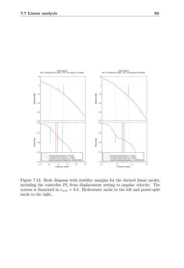
7.7 Linear analysis 93
−200
−150
−100
−50
0
50
Mag
nitu
de (
dB)
10−1
100
101
102
103
104
−270
−225
−180
−135
−90
Pha
se (
deg)
Bode DiagramGm = 50.8 dB (at 40.3 rad/s) , Pm = 67.4 deg (at 1.18 rad/s)
Frequency (rad/s)
Actuator break frequency = 8 rad/sController break frequency = 5 rad/sSystem resonance frequency = 26.6014 rad/s
−200
−150
−100
−50
0
50
Mag
nitu
de (
dB)
10−2
100
102
104
−270
−225
−180
−135
−90
Pha
se (
deg)
Bode DiagramGm = 61.8 dB (at 32 rad/s) , Pm = 33.8 deg (at 0.678 rad/s)
Frequency (rad/s)
Actuator break frequency = 8 rad/sController break frequency = 5 rad/sSystem resonance frequency = 11.2498 rad/s
Figure 7.13: Bode diagram with stability margins for the derived linear model,including the controller PI, from displacement setting to angular velocity. Thesystem is linearised in εm,0 = 0.3. Hydrostatic mode to the left and power-splitmode to the right..
94 Control
When a constant controller is used, the parameters must be adapted for theworst case scenario in order to maintain a stable system, which in this case meanspower-split mode at minimum motor displacement. As a consequence, the con-troller may appear slow in the other operating points. In the controller used inthis thesis, the feed forward signal is however contributing to the major part ofthe total control signal which means that response still is acceptably fast. Anotherway of addressing this issue is to use gain scheduling where the controller gainsare changed depending on operating point [18].
Influence of displacement actuator dynamicsThe speed of the pump and motor actuators are of great importance. A slowactuator will force the phase curve down -90 degrees and a risk of getting a negativephase margin occurs with too slow dynamics. As a consequence, the controllergains cannot be too high without inflicting on stability which in turn degradescontrollability.
Mode shiftThe mode shift event is a delicate and complicated matter within the control. Thecomplications partly inherits from the changes in dynamics when the equivalentinertia changes between the two modes. Another problem is caused by the relayand window effects present in the ”Mode switcher” sub controller. In the idealcase, the clutches are engaged when they are completely synchronised, and in thisexact point both the hydrostatic and the power-split mode demand the exact samespeed from the hydraulic motor. Since the relay and window effects causes themode shift to occur at a speed that deviates somewhat from the theoretical value,a step in the motor reference speed is introduced when the mode is shifted. Thisdisturbance is then magnified by the change in dynamics.
One of the biggest issues during the mode shift however, is the instantaneouschange in load on the hydraulic motor. During hydrostatic mode, all power flowsfrom the diesel engine through the hydrostatic transmission to the wheels. Justafter the mode switch, power-split mode with negative power recirculation is en-tered. This means that the torque on, and thereby the power flow through, themotor changes direction so that the motor starts to work as a pump. Along withthe torque, the pressure sides in the transmission also switches causing the leakagein the circuit to change direction as well.
This changes the control conditions radically, since the integral part has com-pensated for leakage in one direction in hydrostatic mode and then is forced tocompensate for leakage in the other direction in the power-split mode. And dueto the required low integral gain this is not done quickly.
Integrator flip
One way of approaching the issue concerning the rapid change in load discussedabove, is to manipulate the integrator part of the control signal when a mode shiftoccurs. Assuming that the feed forward signal handles the static ideal behaviour
7.7 Linear analysis 95
of the transmission, the integrator signal can be considered to only compensatefor leakage in the transmission circuit. If the leakage after the mode shift is as-sumed to be approximately the same but in the other direction, it would mean thatthe integrator signal should compensate with an equal amount although with theopposite sign. The ”Integrator flip” feature thereby consists of resetting the inte-grator signal, after a mode shift, to the same value as before the mode switch butwith the opposite sign. Thereby, the sudden change in leakage in the transmissionduring a mode shift is compensated for instantaneously in the controller.
This method requires a very accurate feed forward that ensures that the inte-grator only compensates for leakage. If that is not the case, it could actually harmthe control since a big step is introduced in the control signal. In order to achievea more robust and safe control, another solution should be investigated.

96 Control
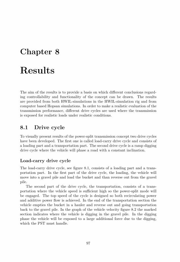
Chapter 8
Results
The aim of the results is to provide a basis on which different conclusions regard-ing controllability and functionality of the concept can be drawn. The resultsare provided from both HWIL-simulations in the HWIL-simulation rig and fromcomputer based Hopsan simulations. In order to make a realistic evaluation of thetransmission performance, different drive cycles are used where the transmissionis exposed for realistic loads under realistic conditions.
8.1 Drive cycleTo visually present results of the power-split transmission concept two drive cycleshave been developed. The first one is called load-carry drive cycle and consists ofa loading part and a transportation part. The second drive cycle is a ramp diggingdrive cycle where the vehicle will phase a road with a constant inclination.
Load-carry drive cycleThe load-carry drive cycle, see figure 8.1, consists of a loading part and a trans-portation part. In the first part of the drive cycle, the loading, the vehicle willmove into a gravel pile and load the bucket and than reverse out from the gravelpile.
The second part of the drive cycle, the transportation, consists of a trans-portation where the vehicle speed is sufficient high so the power-split mode willbe engaged. The top speed of the cycle is designed so both recirculating powerand additive power flow is achieved. In the end of the transportation section thevehicle empties the bucket in a hauler and reverse out and going transportationback to the gravel pile. In the graph of the vehicle velocity figure 8.2 the markedsection indicates where the vehicle is digging in the gravel pile. In the diggingphase the vehicle will be exposed to a large additional force due to the digging,which the PST must handle.
97
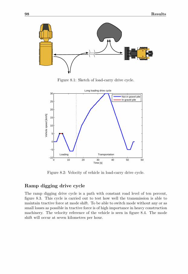
98 Results
Figure 8.1: Sketch of load-carry drive cycle.
0 10 20 30 40 50 60−10
−5
0
5
10
15
20
25
30
Loading Transportation
Long loading drive cycle
Time [s]
Veh
icle
spe
ed [k
m/h
]
Not in gravel pileIn gravel pile
Figure 8.2: Velocity of vehicle in load-carry drive cycle.
Ramp digging drive cycleThe ramp digging drive cycle is a path with constant road level of ten percent,figure 8.3. This cycle is carried out to test how well the transmission is able tomaintain tractive force at mode shift. To be able to switch mode without any or assmall losses as possible in tractive force is of high importance in heavy constructionmachinery. The velocity reference of the vehicle is seen in figure 8.4. The modeshift will occur at seven kilometres per hour.
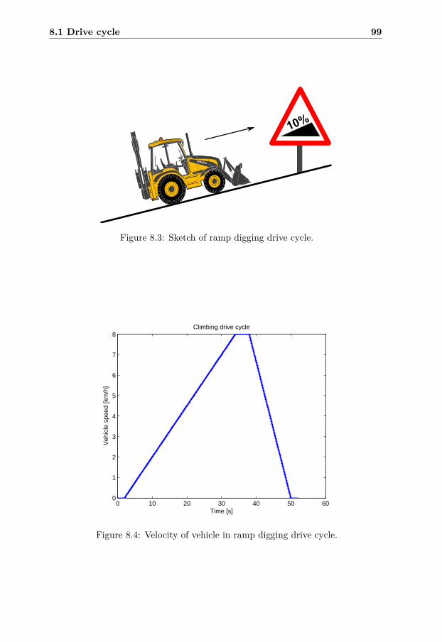
8.1 Drive cycle 99
10%
Figure 8.3: Sketch of ramp digging drive cycle.
0 10 20 30 40 50 600
1
2
3
4
5
6
7
8Climbing drive cycle
Time [s]
Veh
icle
spe
ed [k
m/h
]
Figure 8.4: Velocity of vehicle in ramp digging drive cycle.
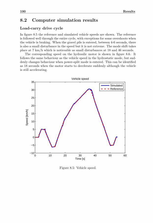
100 Results
8.2 Computer simulation resultsLoad-carry drive cycleIn figure 8.5 the reference and simulated vehicle speeds are shown. The referenceis followed well through the entire cycle, with exceptions for some overshoots whenthe vehicle is braking. When the gravel pile is entered, between 4-6 seconds, thereis also a small disturbance in the speed but it is not extreme. The mode shift takesplace at 7 km/h which is noticeable as small disturbances at 18 and 46 seconds.
The corresponding speed on the hydraulic motor is shown in figure 8.6. Itfollows the same behaviour as the vehicle speed in the hydrostatic mode, but sud-denly changes behaviour when power-split mode is entered. This can be identifiedas 18 seconds when the motor starts to decelerate suddenly although the vehicleis still accelerating.
0 10 20 30 40 50 60−10
−5
0
5
10
15
20
25
30
35Vehicle speed
Time [s]
Spe
ed [k
m/h
]
SimulatedReference
Figure 8.5: Vehicle speed.
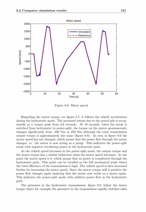
8.2 Computer simulation results 101
0 10 20 30 40 50 60−2500
−2000
−1500
−1000
−500
0
500
1000
1500
2000Motor speed
Time [s]
Spe
ed [r
pm]
SimulatedReference
Figure 8.6: Motor speed.
Regarding the motor torque, see figure 8.7, it follows the vehicle accelerationduring the hydrostatic mode. The increased torque due to the gravel pile is recog-nisable as a torque peak from 4-6 seconds. At 18 seconds, when the mode isswitched from hydrostatic to power-split, the torque on the motor spontaneouslychanges significantly from -100 Nm to 250 Nm although the total transmissionoutput torque is approximately the same (figure 8.8). As seen in figure 8.6 themotor speed has not changed, which means that the power flow through the motorchanges, i.e. the motor is now acting as a pump. This indicates the power-splitmode with negative circulating power in the hydrostatic path.
As the vehicle speed increases in the power-split mode, the output torque andthe motor torque has a similar behaviour when the motor speed increases. At onepoint the motor speed is 0, which means that no power is transferred through thehydrostatic path. This point can be recalled as the full mechanical point wherethe total efficiency of the transmission is high. The vehicle speed is then increasedfurther by increasing the motor speed. Since the motor torque still is positive thepower flow changes again implying that the motor now works as a motor again.This indicates the power-split mode with additive power flow in the hydrostaticpath.
The pressures in the hydrostatic transmission, figure 8.9, follow the motortorque where for example the pressures in the transmission rapidly switches sides
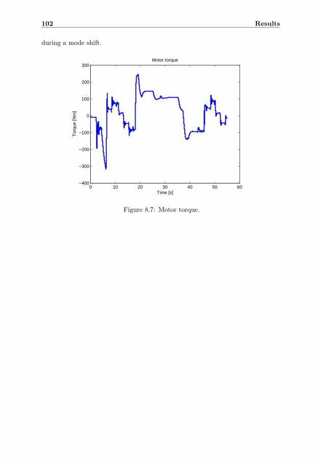
102 Results
during a mode shift.
0 10 20 30 40 50 60−400
−300
−200
−100
0
100
200
300Motor torque
Time [s]
Tor
que
[Nm
]
Figure 8.7: Motor torque.
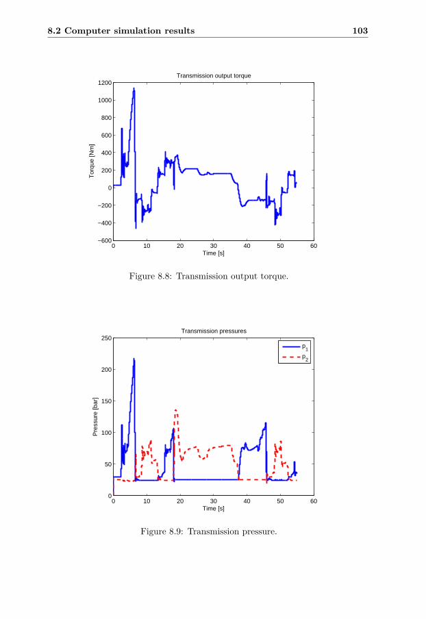
8.2 Computer simulation results 103
0 10 20 30 40 50 60−600
−400
−200
0
200
400
600
800
1000
1200Transmission output torque
Time [s]
Tor
que
[Nm
]
Figure 8.8: Transmission output torque.
0 10 20 30 40 50 600
50
100
150
200
250Transmission pressures
Time [s]
Pre
ssur
e [b
ar]
p
1
p2
Figure 8.9: Transmission pressure.
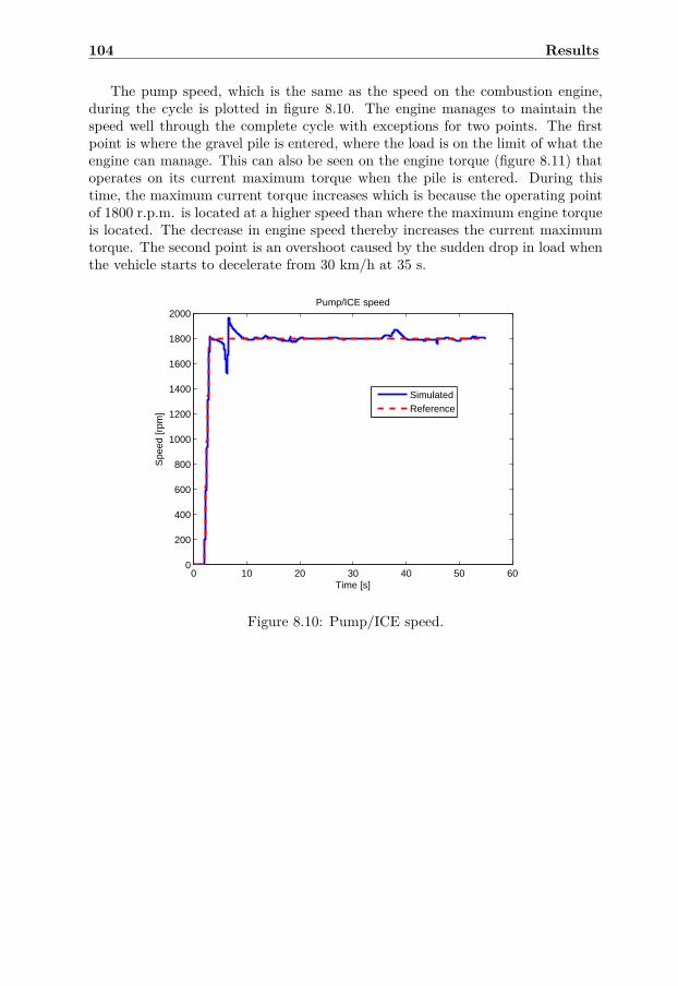
104 Results
The pump speed, which is the same as the speed on the combustion engine,during the cycle is plotted in figure 8.10. The engine manages to maintain thespeed well through the complete cycle with exceptions for two points. The firstpoint is where the gravel pile is entered, where the load is on the limit of what theengine can manage. This can also be seen on the engine torque (figure 8.11) thatoperates on its current maximum torque when the pile is entered. During thistime, the maximum current torque increases which is because the operating pointof 1800 r.p.m. is located at a higher speed than where the maximum engine torqueis located. The decrease in engine speed thereby increases the current maximumtorque. The second point is an overshoot caused by the sudden drop in load whenthe vehicle starts to decelerate from 30 km/h at 35 s.
0 10 20 30 40 50 600
200
400
600
800
1000
1200
1400
1600
1800
2000Pump/ICE speed
Time [s]
Spe
ed [r
pm]
SimulatedReference
Figure 8.10: Pump/ICE speed.
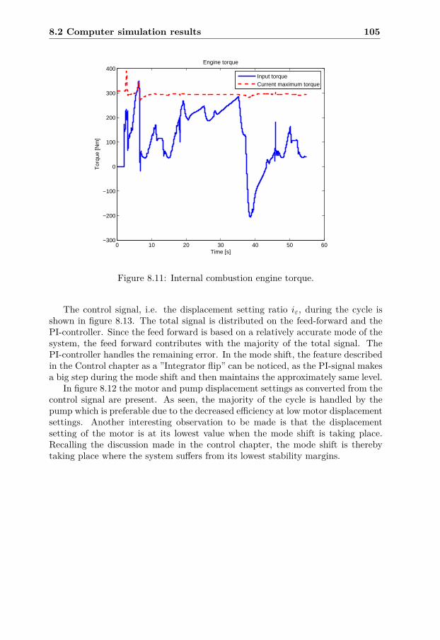
8.2 Computer simulation results 105
0 10 20 30 40 50 60−300
−200
−100
0
100
200
300
400Engine torque
Time [s]
Tor
que
[Nm
]
Input torqueCurrent maximum torque
Figure 8.11: Internal combustion engine torque.
The control signal, i.e. the displacement setting ratio iε, during the cycle isshown in figure 8.13. The total signal is distributed on the feed-forward and thePI-controller. Since the feed forward is based on a relatively accurate mode of thesystem, the feed forward contributes with the majority of the total signal. ThePI-controller handles the remaining error. In the mode shift, the feature describedin the Control chapter as a ”Integrator flip” can be noticed, as the PI-signal makesa big step during the mode shift and then maintains the approximately same level.
In figure 8.12 the motor and pump displacement settings as converted from thecontrol signal are present. As seen, the majority of the cycle is handled by thepump which is preferable due to the decreased efficiency at low motor displacementsettings. Another interesting observation to be made is that the displacementsetting of the motor is at its lowest value when the mode shift is taking place.Recalling the discussion made in the control chapter, the mode shift is therebytaking place where the system suffers from its lowest stability margins.
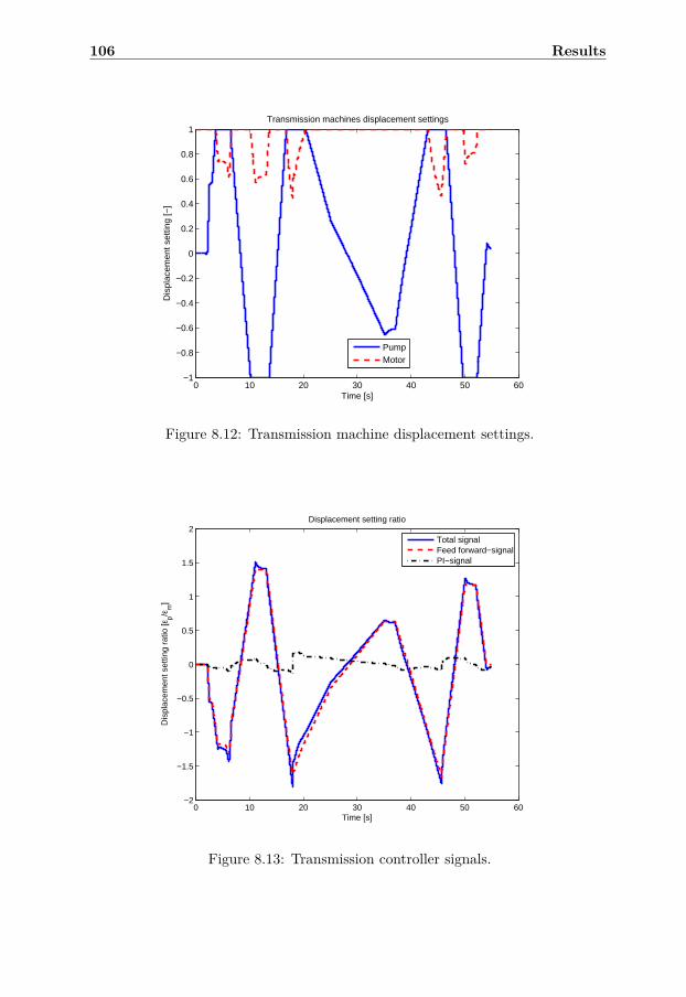
106 Results
0 10 20 30 40 50 60−1
−0.8
−0.6
−0.4
−0.2
0
0.2
0.4
0.6
0.8
1Transmission machines displacement settings
Time [s]
Dis
plac
emen
t set
ting
[−]
PumpMotor
Figure 8.12: Transmission machine displacement settings.
0 10 20 30 40 50 60−2
−1.5
−1
−0.5
0
0.5
1
1.5
2Displacement setting ratio
Time [s]
Dis
plac
emen
t set
ting
ratio
[εp/ε
m]
Total signalFeed forward−signalPI−signal
Figure 8.13: Transmission controller signals.
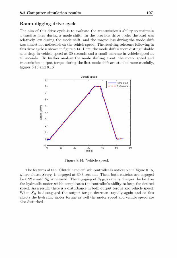
8.2 Computer simulation results 107
Ramp digging drive cycleThe aim of this drive cycle is to evaluate the transmission’s ability to maintaina tractive force during a mode shift. In the previous drive cycle, the load wasrelatively low during the mode shift, and the torque loss during the mode shiftwas almost not noticeable on the vehicle speed. The resulting reference following inthis drive cycle is shown in figure 8.14. Here, the mode shift is more distinguishableas a drop in vehicle speed at 30 seconds and a small increase in vehicle speed at40 seconds. To further analyse the mode shifting event, the motor speed andtransmission output torque during the first mode shift are studied more carefully,figures 8.15 and 8.16.
0 10 20 30 40 50 60−1
0
1
2
3
4
5
6
7
8
9Vehicle speed
Time [s]
Spe
ed [k
m/h
]
SimulatedReference
Figure 8.14: Vehicle speed.
The features of the ”Clutch handler” sub controller is noticeable in figure 8.16,where clutch SF W D is engaged at 30.3 seconds. Then, both clutches are engagedfor 0.22 s until SH is released. The engaging of SF W D rapidly changes the load onthe hydraulic motor which complicates the controller’s ability to keep the desiredspeed. As a result, there is a disturbance in both output torque and vehicle speed.When SH is disengaged the output torque decreases rapidly again and as thisaffects the hydraulic motor torque as well the motor speed and vehicle speed arealso disturbed.
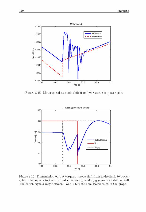
108 Results
30 30.2 30.4 30.6 30.8 31−2060
−2050
−2040
−2030
−2020
−2010
−2000
−1990Motor speed
Time [s]
Spe
ed [r
pm]
SimulatedReference
Figure 8.15: Motor speed at mode shift from hydrostatic to power-split.
30 30.2 30.4 30.6 30.8 31250
300
350
400
450
500Transmission output torque
Time [s]
Tor
que
[Nm
]
Output torqueS
H
SFWD
Figure 8.16: Transmission output torque at mode shift from hydrostatic to power-split. The signals to the involved clutches SH and SF W D are included as well.The clutch signals vary between 0 and 1 but are here scaled to fit in the graph.
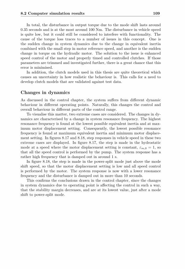
8.2 Computer simulation results 109
In total, the disturbance in output torque due to the mode shift lasts around0.35 seconds and is at the most around 100 Nm. The disturbance in vehicle speedis quite low, but it could still be considered to interfere with functionality. Thecause of the torque loss traces to a number of issues in this concept. One isthe sudden change in system dynamics due to the change in equivalent inertiacombined with the small step in motor reference speed, and another is the suddenchange in torque on the hydraulic motor. The solution to the issue is enhancedspeed control of the motor and properly timed and controlled clutches. If thoseparameters are trimmed and investigated further, there is a great chance that thiserror is minimised.
In addition, the clutch models used in this thesis are quite theoretical whichcauses an uncertainty in how realistic the behaviour is. This calls for a need todevelop clutch models that are validated against test data.
Changes in dynamicsAs discussed in the control chapter, the system suffers from different dynamicbehaviour in different operating points. Naturally, this changes the control andoverall behaviour in different parts of the control range.
To visualise this matter, two extreme cases are considered. The changes in dy-namics are characterised by a change in system resonance frequency. The highestresonance frequency is found at the lowest possible equivalent inertia and at max-imum motor displacement setting. Consequently, the lowest possible resonancefrequency is found at maximum equivalent inertia and minimum motor displace-ment setting. In figures 8.17 and 8.18, step responses in vehicle speed in these twoextreme cases are displayed. In figure 8.17, the step is made in the hydrostaticmode at a speed where the motor displacement setting is constant, εm,0 = 1, sothat all the speed control is performed by the pump. The system response has arather high frequency that is damped out in around 1 s.
In figure 8.18, the step is made in the power-split mode just above the modeshift speed, so that the motor displacement setting is low and all speed controlis performed by the motor. The system response is now with a lower resonancefrequency and the disturbance is damped out in more than 10 seconds.
This confirms the conclusions drawn in the control chapter, since the changesin system dynamics due to operating point is affecting the control in such a way,that the stability margin decreases, and are at its lowest value, just after a modeshift to power-split mode.
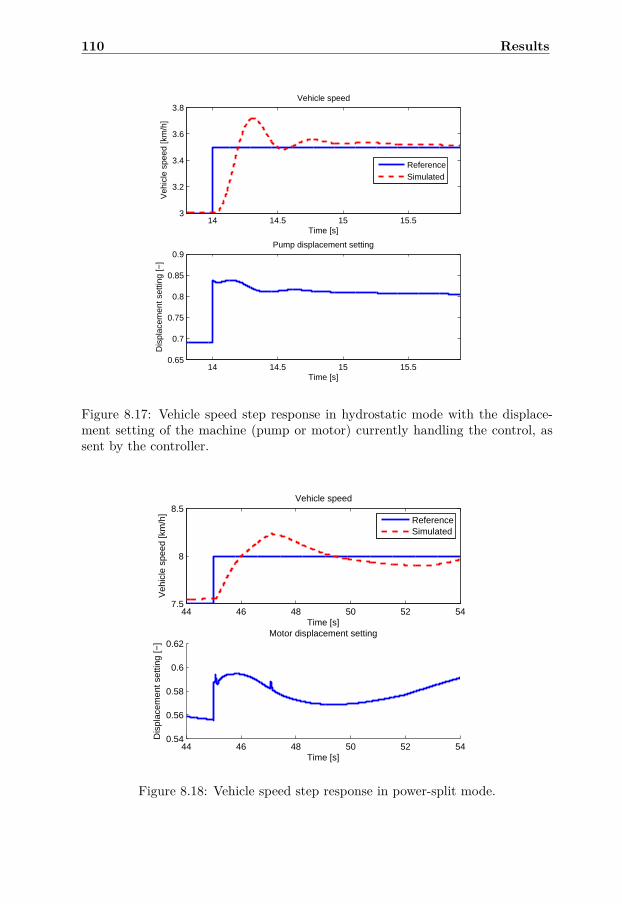
110 Results
14 14.5 15 15.53
3.2
3.4
3.6
3.8Vehicle speed
Time [s]
Veh
icle
spe
ed [k
m/h
]
ReferenceSimulated
14 14.5 15 15.50.65
0.7
0.75
0.8
0.85
0.9Pump displacement setting
Time [s]
Dis
plac
emen
t set
ting
[−]
Figure 8.17: Vehicle speed step response in hydrostatic mode with the displace-ment setting of the machine (pump or motor) currently handling the control, assent by the controller.
44 46 48 50 52 547.5
8
8.5Vehicle speed
Time [s]
Veh
icle
spe
ed [k
m/h
]
ReferenceSimulated
44 46 48 50 52 540.54
0.56
0.58
0.6
0.62Motor displacement setting
Time [s]
Dis
plac
emen
t set
ting
[−]
Figure 8.18: Vehicle speed step response in power-split mode.
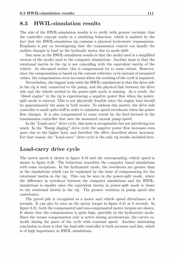
8.3 HWIL-simulation results 111
8.3 HWIL-simulation resultsThe aim of the HWIL-simulation results is to verify with greater certainty thatthe controller concept works in a satisfying behaviour, which is enabled by thefact that the HWIL-simulation rig contains a physical hydrostatic transmission.Emphasis is put on investigating that the transmission control can handle thesudden changes in load on the hydraulic motor due to mode shift.
One issue in the HWIL-simulation results is that the model used is a simplifiedversion of the model used in the computer simulations. Another issue is that therotational inertia in the rig is not coinciding with the equivalent inertia of thevehicle. As discussed earlier, this is compensated for to some extent. However,since the compensation is based on the current reference cycle instead of measuredvalues, the compensation error increases when the tracking of the cycle is impaired.
Nevertheless, the biggest issue with the HWIL-simulations is that the drive sidein the rig is only connected to the pump, and the physical link between the driveside and the wheels needed in the power-split mode is missing. As a result, the”diesel engine” in the rig is experiencing a negative power flow when the power-split mode is entered. This is not physically feasible since the engine load shouldbe approximately the same in both modes. To address this matter, the drive sidecontroller is made quite stiff in order to minimise speed overshoots when the powerflow changes. It is also compensated to some extent by the feed forward in thetransmission controller that uses the measured current pump speed.
In the ”Load-carry” drive cycle, this issue is recognisable but not interfering toomuch. In the ”Ramp digging” drive cycle the negative power flow increases evenmore due to the higher load, and therefore the effect described above increases.For that reason, the ”Load-carry” drive cycle is the only rig results included here.
Load-carry drive cycleThe motor speed is shown in figure 8.19 and the corresponding vehicle speed isshown in figure 8.20. The behaviour resembles the computer based simulationswith some exceptions. In the hydrostatic mode, the overshoots are greater thanin the simulations which can be explained by the issue of compensating for therotational inertia in the rig. This can be seen in the power-split mode, wherethe difference in overshoot between the computer simulations and the HWIL-simulations is smaller since the equivalent inertia in power-split mode is closerto the rotational inertia in the rig. The greater variation in pump speed alsocontributes.
The gravel pile is recognised as a motor and vehicle speed disturbance at 8seconds. It can also be seen on the motor torque in figure 8.21 at 8 seconds. Infigure 8.21, both the compensated and non-compensated motor torques are shown.It shows that the compensation is quite high, specially in the hydrostatic mode.Since the torque compensation only is active during accelerations, the curves co-incide during the parts of the cycle with constant speed. Another interestingconclusion to draw is that the load side controller is both accurate and fast, whichis of high importance in HWIL simulations.
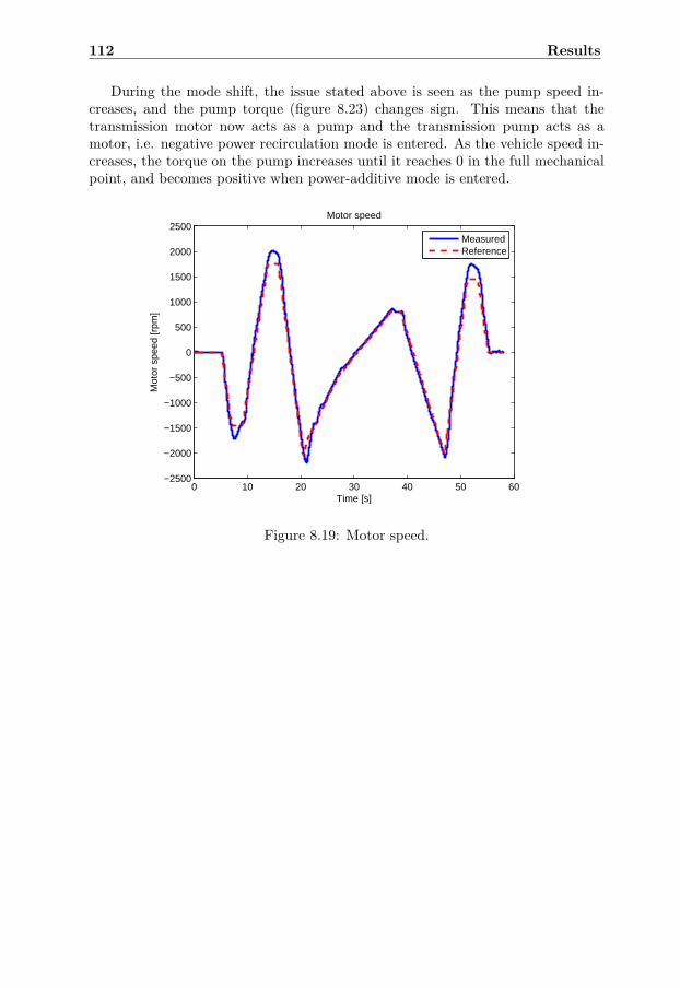
112 Results
During the mode shift, the issue stated above is seen as the pump speed in-creases, and the pump torque (figure 8.23) changes sign. This means that thetransmission motor now acts as a pump and the transmission pump acts as amotor, i.e. negative power recirculation mode is entered. As the vehicle speed in-creases, the torque on the pump increases until it reaches 0 in the full mechanicalpoint, and becomes positive when power-additive mode is entered.
0 10 20 30 40 50 60−2500
−2000
−1500
−1000
−500
0
500
1000
1500
2000
2500
Time [s]
Mot
or s
peed
[rpm
]
Motor speed
MeasuredReference
Figure 8.19: Motor speed.
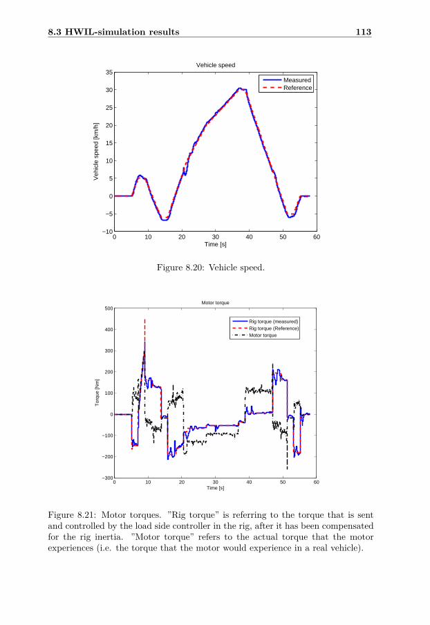
8.3 HWIL-simulation results 113
0 10 20 30 40 50 60−10
−5
0
5
10
15
20
25
30
35
Veh
icle
spe
ed [k
m/h
]
Time [s]
Vehicle speed
MeasuredReference
Figure 8.20: Vehicle speed.
0 10 20 30 40 50 60−300
−200
−100
0
100
200
300
400
500
Time [s]
Tor
que
[Nm
]
Motor torque
Rig torque (measured)Rig torque (Reference)Motor torque
Figure 8.21: Motor torques. ”Rig torque” is referring to the torque that is sentand controlled by the load side controller in the rig, after it has been compensatedfor the rig inertia. ”Motor torque” refers to the actual torque that the motorexperiences (i.e. the torque that the motor would experience in a real vehicle).

114 Results
The sudden change in load conditions at the mode shift disturbs the transmis-sion speed controller which is noticeable in both motor speed and vehicle speed.This disturbance is greater here than in the computer simulations which can beexplained by several factors, such as the inertia compensation and model error.The biggest error is though probably due to the missing physical link between thedrive side and the wheels, as it changes the drive side behaviour significantly.
The transmission pressures, figure 8.24, follow the load on the motor. Thepressure oscillations are greater here than in the computer simulations which mostlikely is due to model errors and errors in the inertia compensation.
0 10 20 30 40 50 601600
1650
1700
1750
1800
1850
1900
1950
2000
Time [s]
Pum
p sp
eed
[rpm
]
Pump speed
Figure 8.22: Pump/engine speed.
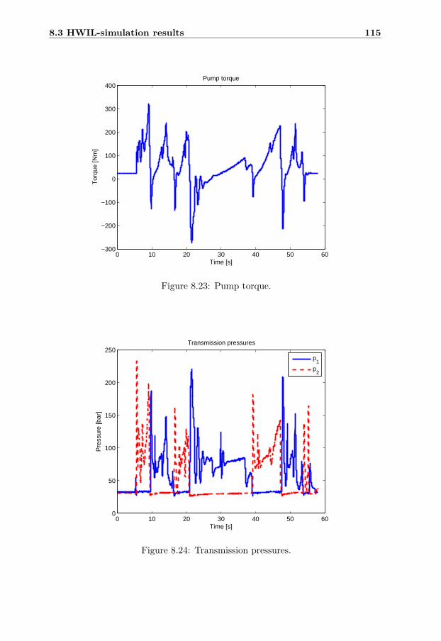
8.3 HWIL-simulation results 115
0 10 20 30 40 50 60−300
−200
−100
0
100
200
300
400
Time [s]
Tor
que
[Nm
]
Pump torque
Figure 8.23: Pump torque.
0 10 20 30 40 50 600
50
100
150
200
250
Time [s]
Pre
ssur
e [b
ar]
Transmission pressures
p
1
p2
Figure 8.24: Transmission pressures.
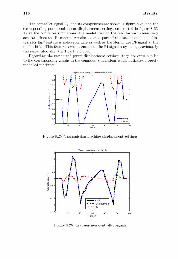
116 Results
The controller signal, iε, and its components are shown in figure 8.26, and thecorresponding pump and motor displacement settings are plotted in figure 8.25.As in the computer simulations, the model used in the feed forward seems veryaccurate since the PI-controller makes a small part of the total signal. The ”In-tegrator flip” feature is noticeable here as well, as the step in the PI-signal at themode shifts. This feature seems accurate as the PI-signal stays at approximatelythe same value after the I-part is flipped.
Regarding the motor and pump displacement settings, they are quite similarto the corresponding graphs in the computer simulations which indicates properlymodelled machines.
0 10 20 30 40 50 60−1
−0.8
−0.6
−0.4
−0.2
0
0.2
0.4
0.6
0.8
1
Time [s]
Dis
plac
emen
t set
ting
[−]
Displacement setting of transmission machines
PumpMotor
Figure 8.25: Transmission machine displacement settings.
0 10 20 30 40 50 60−2.5
−2
−1.5
−1
−0.5
0
0.5
1
1.5
2
Time [s]
Con
trol
sig
nal [
−]
Transmission control signals
TotalFeed−forwardPID
Figure 8.26: Transmission controller signals.
Chapter 9
Summary and Conclusions
The purpose of the thesis is to investigate and evaluate the 2-mode Jarchow power-split transmission concept for a Volvo Backhoe loader out of a control perspectiveand an energy efficiency perspective. The results show that the concept could bean alternative to the current concept, and that it is sufficiently effective to enableengine downsizing from 64 kW to 55 kW when it comes to reaching maximumvelocity and maximum tractive force at standstill. A drawback with the smallerengine is however the lowered tractive force at medium speeds compared to theconventional concept, which could limit the vehicle performance in some cases.
The complete studied system, i.e. driveline and vehicle, have been modelledand the components of greatest complexity, namely the hydrostatic transmission,have been validated against data from a test rig including a physical hydrostatictransmission. By also using the same rig for HWIL-simulations the reliability ofthe results increases further. Furthermore, the system has been analysed from acontrol perspective and a control concept has been developed, implemented andevaluated for the transmission concept.
Regarding the controllability, the results show that the studied concept is con-trollable in a tolerable manner as long as the involved clutches and the hydrostatictransmission are controlled properly. This require a fast controller and fast re-sponses in the hydrostatic machines. Issues that arise in the transmission controlare mainly concentrated in the mode shifting event, where the dynamics of thesystem changes simultaneously with the external load on the hydrostatic trans-mission. The consequence of improper speed and clutch control during the modeshift is issues in maintaining the tractive force. This matter is linked to function-ality and is of high importance in heavy construction machinery. Thereby, thespeed control can be viewed as the essence of realising this concept into a physicaltransmission.
117

118 Summary and Conclusions
Chapter 10
Future work
• Evaluate a hybrid concept. This could also be implemented in the HWIL-simulation rig thanks to the hydraulic accumulators installed.
• Investigate an option to the ”Integrator flip” feature in the controller in orderto improve the transmission control during mode shift.
• Implement a torque based controller in the HWIL-simulation rig so that acombustion engine can be simulated more properly.
• Add an accelerometer to the load side on the HWIL-simulation rig in orderto enhance the inertia simulation.
• Investigate the possibility to implement a physically variable inertia on theload side in the rig.
• Add a possibility to provide an external torque on the drive side on theHWIL-simulation rig so that the physical link between the wheels and theengine in the power-split mode can be simulated in a more realistic way.
119

120 Future work
Chapter 11
Appendix
11.1 Models
11.2 Qt Creator Models
Simple clutch
#ifndef SIMPLE_CLUTCH_C_H#define SIMPLE_CLUTCH_C_H#include <math . h>#include " ComponentEssentials . h "#include " ComponentUt i l i t i e s . h "
us ing namespace std ;
namespace hopsan {
c l a s s Simple_clutch_C : pub l i c ComponentC{
pr i va t e :double k ,X,T_f , alpha , c10 , c20 , Type ;double w1 , c1 , l a s t c1 , w2 , c2 , l a s t c2 , Zx ;double ∗mpND_w1, ∗mpND_c1, ∗mpND_Zx1, ∗mpND_w2, ∗
mpND_c2, ∗mpND_Zx2,∗mpX;Port ∗mpP1, ∗mpP2;
pub l i c :stat ic Component ∗Creator ( )
121
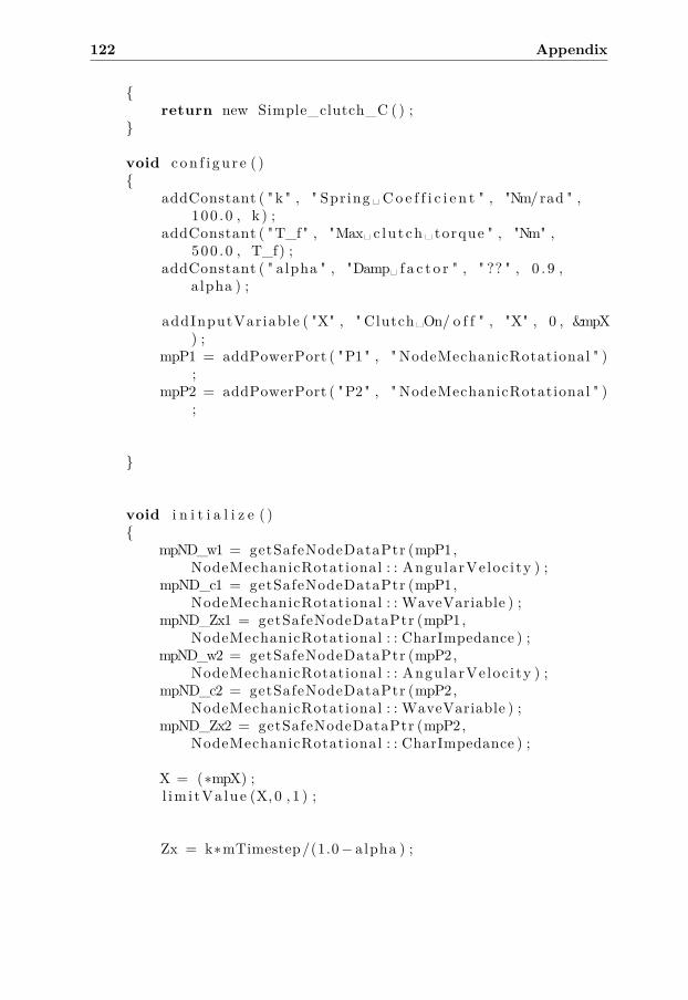
122 Appendix
{return new Simple_clutch_C ( ) ;
}
void c on f i gu r e ( ){
addConstant ( " k " , " Spring ␣ Co e f f i c i e n t " , "Nm/rad " ,100 .0 , k ) ;
addConstant ( "T_f" , "Max␣ c lu t ch ␣ torque " , "Nm" ,500 .0 , T_f) ;
addConstant ( " alpha " , "Damp␣ f a c t o r " , " ?? " , 0 . 9 ,alpha ) ;
addInputVariable ( "X" , " Clutch␣On/ o f f " , "X" , 0 , &mpX) ;
mpP1 = addPowerPort ( "P1" , " NodeMechanicRotational " );
mpP2 = addPowerPort ( "P2" , " NodeMechanicRotational " );
}
void i n i t i a l i z e ( ){
mpND_w1 = getSafeNodeDataPtr (mpP1,NodeMechanicRotational : : AngularVeloc i ty ) ;
mpND_c1 = getSafeNodeDataPtr (mpP1,NodeMechanicRotational : : WaveVariable ) ;
mpND_Zx1 = getSafeNodeDataPtr (mpP1,NodeMechanicRotational : : CharImpedance ) ;
mpND_w2 = getSafeNodeDataPtr (mpP2,NodeMechanicRotational : : AngularVeloc i ty ) ;
mpND_c2 = getSafeNodeDataPtr (mpP2,NodeMechanicRotational : : WaveVariable ) ;
mpND_Zx2 = getSafeNodeDataPtr (mpP2,NodeMechanicRotational : : CharImpedance ) ;
X = (∗mpX) ;l im i tVa lue (X, 0 , 1 ) ;
Zx = k∗mTimestep/(1.0− alpha ) ;
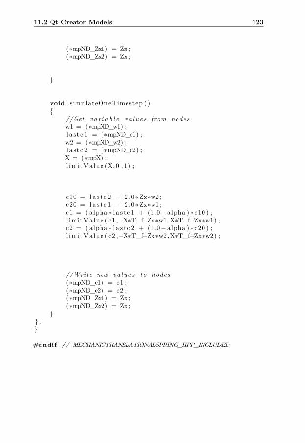
11.2 Qt Creator Models 123
(∗mpND_Zx1) = Zx ;(∗mpND_Zx2) = Zx ;
}
void simulateOneTimestep ( ){
//Get v a r i a b l e va l u e s from nodesw1 = (∗mpND_w1) ;l a s t c 1 = (∗mpND_c1) ;w2 = (∗mpND_w2) ;l a s t c 2 = (∗mpND_c2) ;X = (∗mpX) ;l im i tVa lue (X, 0 , 1 ) ;
c10 = l a s t c 2 + 2.0∗Zx∗w2 ;c20 = l a s t c 1 + 2.0∗Zx∗w1 ;c1 = ( alpha ∗ l a s t c 1 + (1.0− alpha ) ∗ c10 ) ;l im i tVa lue ( c1 ,−X∗T_f−Zx∗w1 ,X∗T_f−Zx∗w1) ;c2 = ( alpha ∗ l a s t c 2 + (1.0− alpha ) ∗ c20 ) ;l im i tVa lue ( c2 ,−X∗T_f−Zx∗w2 ,X∗T_f−Zx∗w2) ;
//Write new va l ue s to nodes(∗mpND_c1) = c1 ;(∗mpND_c2) = c2 ;(∗mpND_Zx1) = Zx ;(∗mpND_Zx2) = Zx ;
}} ;}
#endif // MECHANICTRANSLATIONALSPRING_HPP_INCLUDED

124 Appendix
Bibliography
[1] Hydraulic hybrid transmission - project report. Student project, IEI,Linköping University, 2014.
[2] http://www.iei.liu.se/flumes/system-simulation/hopsanng/. Linköping Uni-versity, Division of Fluid and Mechatronic Systems, Feb. 2014.
[3] Institutionen för konstruktions-och produktionsteknik. Formelsamling i Hy-draulik och Pneumatik. Linköpings Tekniska Högskola, 1995.
[4] Karl-Erik Rydberg. Hydrostatic Drives in Heavy Mobile Machine - New Con-cept and Development Trends. Technical report, Department of Managementand Engineering, Linköping University, 1997.
[5] Mikael Sannelius. On Complex Hydrostatic Transmissions, Design of a Two-Motor Concept using Computer Aided Development Tools. PhD thesis,Linköping University, 1999.
[6] K. Williams B. Carl, M. Ivantysynova. Comparison of Operational Charac-teristics in Power Split Continuously Variable Transmissions. CommercialVehicle Engineering Congress and Exhibition, 2006, Hannover, Germany.
[7] K. T. Renius and R. Resch. Continuously variable tractor transmissions.ASAE Distinguished Lecture Series Tractor design No. 29, 2005.
[8] K. Pettersson. Design Automation of Complex Hydromechanical Transmis-sions. PhD thesis, Linköping University, 2013.
[9] J. H. Kress. Hydrostatic Power-Splitting Transmissions for Wheeled Vehicle- Classificatuion and Theory Operation. SAE Technical Paper, 1968.
[10] Rajneesh Kumar. A Power Management Strategy for Hybrid Output CoupledPower-split Transmission to Minimize Fuel Consumption. PhD thesis, PurdueUniversity, 2010.
[11] F. Jarchow et al. ”Continuous-Acting Hydrostatic-Mechanical Power-ShiftTransmission With Toothed Clutches”. US5,052,986. 1991.
[12] Erik Forsberg Stefan Ekström. Modelling and Control of Hydrostatic Trans-mission for Construction Machine. Master’s thesis, Linköping University,2010.
125
126 Bibliography
[13] Shiva Kumar BM et al. Implementation of control system for hydrostatictransmission test rig - project report. Student project, IEI, Linköping Uni-versity, 2010.
[14] Robert Braun. Multi-Threaded Distributed System Simulations - Using Bi-Lateral Delay Lines. Licentiate thesis, Linköping University, 2013.
[15] Göran Palmgren. ON SECONDARY CONTROLLED HYDRAULIC SYS-TEMS. PhD thesis, Linköping University, 1988.
[16] Karl-Erik Rydberg. On performance optimization and digital control of hy-drostatic drives for vehicle applications. PhD thesis, Linköping University,1983.
[17] Torsten Kohmäscher et al. Design, analysis, control and diagnosis of fluidpower systems. In International Mechanical Engineering Congress and Expo-sition, 2007, Seattle, Washington USA.
[18] Jerker Lennevi. Hydrostatic Transmission Control. PhD thesis, LinköpingUniversity, 1995.