simulation and experimental investigations of co injection ... · conventional (wellman unit) ......
TRANSCRIPT
Simulation and Experimental Investigations of CO2 Injection in Both
Conventional (Wellman Unit) and Unconventional Reservoirs
Department of Petroleum Engineering
Texas A&M University
Dr. David Schechter
19th Annual CO2 Flooding Conference
Midland, TX
December 12th, 2013

CO2 Oil Recovery
Observations
• CO2 EOR recovers oil very effectively • It’s limited by the availability of CO2
• The laboratory and simulation research technology is aimed at improving the utilization of CO2 (areal and vertical sweep efficiency) through mobility control)
• Research into gravity stable floods (Wellman Unit) • The research technology is improving prediction of processing
rates (net utilization and gross utilization - Mscf CO2/bbl EOR) with dimensionless curves for H2O and CO2
• The big prize is utilizing CO2 in the ROZ & countless “boom” wells in unconventional liquid reservoirs (ULR)

Mobility Control with Viscosifier Sweep Efficiency after 0.5 PV Injected
Pure CO2
Dodecamethylpentasiloxane Viscosified CO2 Flood
Fracture
Shuzong Cai, 2011

Bottom Water Drive
Original Reservoir Conditions
Sec. Gas
Cap
Prod Prod
Bottom Water Drive
Before Waterflooding (1979)
Prod Prod
WIW WIW
Bottom Water Drive
Waterflooding (Before CO 2 Flood),1983
CO2 ICO2 I
WIWWIW
Prod Prod
Waterflood and CO2 Injection (1995)
Bottom Water Drive
Bottom Water Drive
Original Reservoir Conditions
Bottom Water Drive
Original Reservoir Conditions
Sec. Gas
Cap
Prod Prod
Bottom Water Drive
Before Waterflooding (1979)
Prod Prod
WIW WIW
Bottom Water Drive
Waterflooding (Before CO 2 Flood),1983
CO2 ICO2 I
WIWWIW
Prod Prod
Waterflood and CO2 Injection (1995)
Bottom Water Drive
CO2 ICO2 I
WIWWIW
Prod Prod
Waterflood and CO2 Injection (1995)
Bottom Water Drive
WIWWIW
Prod Prod
Waterflood and CO2 Injection (1995)
Bottom Water Drive
Bottom Water Drive
Original Reservoir Conditions
Bottom Water Drive
Original Reservoir Conditions
Sec. Gas
Cap
Prod Prod
Bottom Water Drive
Before Waterflooding (1979)
Prod Prod
WIW WIW
Bottom Water Drive
Waterflooding (Before CO 2 Flood),1983
CO2 ICO2 I
WIWWIW
Prod Prod
Waterflood and CO2 Injection (1995)
Bottom Water Drive
WIWWIW
Prod Prod
Waterflood and CO2 Injection (1995)
Bottom Water Drive
CO2 ICO2 I
WIWWIW
Prod Prod
Waterflood and CO2 Injection (1995)
Bottom Water Drive
WIWWIW
Prod Prod
Waterflood and CO2 Injection (1995)
Bottom Water Drive
Chronological Stages of Depletion
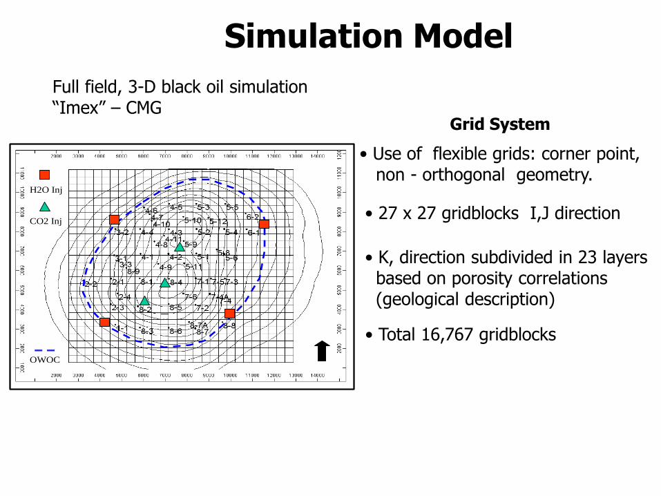
Simulation Model
H2O Inj
CO2 Inj
OWOC
H2O Inj
CO2 Inj
OWOC
H2O Inj
CO2 Inj
OWOC
Grid System
• Use of flexible grids: corner point, non - orthogonal geometry.
• K, direction subdivided in 23 layers based on porosity correlations (geological description)
• 27 x 27 gridblocks I,J direction
Full field, 3-D black oil simulation “Imex” – CMG
• Total 16,767 gridblocks

Permeability
• Use previous estimations from correlations between open logs and core measurements
K = 10^(0.167 * Core porosity – 0.537)
• Relationship may not be representative due to fractures and vugular porosity
Water Saturation
Simulation Model Input Data
Swc, aprox 20% for Ф = 8.5%Swc, aprox 20% for Ф = 8.5%

• Use of isopach maps resulted from geological and petrophysical study in 1994
• Geological and stratigraphic correlation (Core vs Log data) • Quantify major rock properties • Lateral and areal continuity
Isopach Maps
• 60 geological contoured maps from gross thickness, porosity and NTGR were digitized • Interpolation between contour allows model to be populated
Gross Thickness Porosity Net to Gross Ratio
Simulation Model Input Data
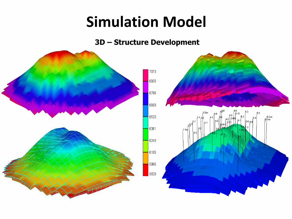
Simulation Model 3D – Structure Development

Measured BHP’s for History Matching
Production data
• Over 45 years of monthly cumulative oil, gas and water production from 47 wells was converted into daily rate schedules for simulation
• Model initially constrained by oil rates and water/CO2 injection rates
Pressure data
• Pressure measurements reveal good communication within the reservoir • Use of BHP corrected and averaged to a common mid-perforation • Static BHP seemed to be representative of the average reservoir pressure
0
500
1,000
1,500
2,000
2,500
3,000
3,500
4,000
4,500
A-49 M-53 J-57 A-61 S-65 O-69 D-73 J-78 F-82 M-86 M-90 J-94
Time, years
Bo
tto
m H
ole
Pre
ssu
re
(BH
P),
P
si
Unit 1-1 Unit 2-1 Unit 2-3 Unit 3-3 Unit 4-1 Unit 4-2
Unit 4-3 Unit 4-4 Unit 4-5 Un it 4-6 Unit 4-7 Unit 5-1
Unit 5-2 Unit 5-3 Unit 5-4 Unit 5-5 Unit 6-1 Unit 6-2
Unit 7-1 Unit 7-2 Unit 8-3 Unit 8-5 Unit 8-6 Unit 8-7A
Individual Static Bottom Hole Pressure
a)
b)
c)
1979
1983
1995
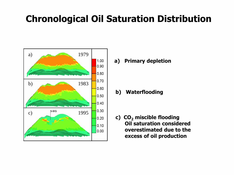
Chronological Oil Saturation Distribution
a) Primary depletion
b) Waterflooding
c) CO2 miscible flooding Oil saturation considered overestimated due to the excess of oil production

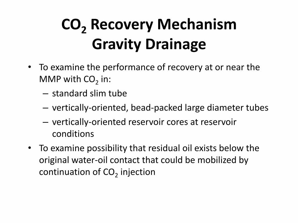
CO2 Recovery Mechanism Gravity Drainage
• To examine the performance of recovery at or near the MMP with CO2 in:
– standard slim tube
– vertically-oriented, bead-packed large diameter tubes
– vertically-oriented reservoir cores at reservoir conditions
• To examine possibility that residual oil exists below the original water-oil contact that could be mobilized by continuation of CO2 injection
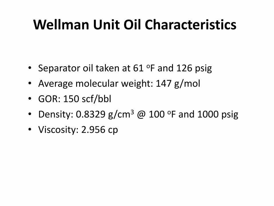
Wellman Unit Oil Characteristics
• Separator oil taken at 61 oF and 126 psig
• Average molecular weight: 147 g/mol
• GOR: 150 scf/bbl
• Density: 0.8329 g/cm3 @ 100 oF and 1000 psig
• Viscosity: 2.956 cp
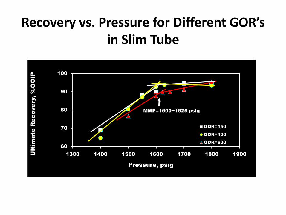
Recovery vs. Pressure for Different GOR’s in Slim Tube
60
70
80
90
100
1300 1400 1500 1600 1700 1800 1900Ultim
ate
R
ec
ove
ry, %
OO
IP
Pressure, psig
GOR=150
GOR=400
GOR=600
MMP=1600~1625 psig

Recovery Curves for Each Large Diameter Tube Test
0
20
40
60
80
100
120
0 20 40 60 80 100 120 140 160 180
% O
OIP
P
ro
du
ce
d O
il
% OOIP of CO2 Injected
Run A: 1700 psig / gravity stable
Run B: 1550 psig / gravity stable
Run C: 1400 psig / gravity stable
Run D: 1700 psig / gravity stable
Run E: 1400 psig / gravity unstable
Run F: 1400 psig / horizontal

Cores From Wellman 5-10
• 30’ whole core from 9400’ to 9430’
• 26 samples for standard core analysis
• 3’ section for gravity stable CO2 tests
• Helium porosities: 2.4% ~ 12.6%
• Average porosity: 5.8% for 26 samples
• Average water saturation: 42%
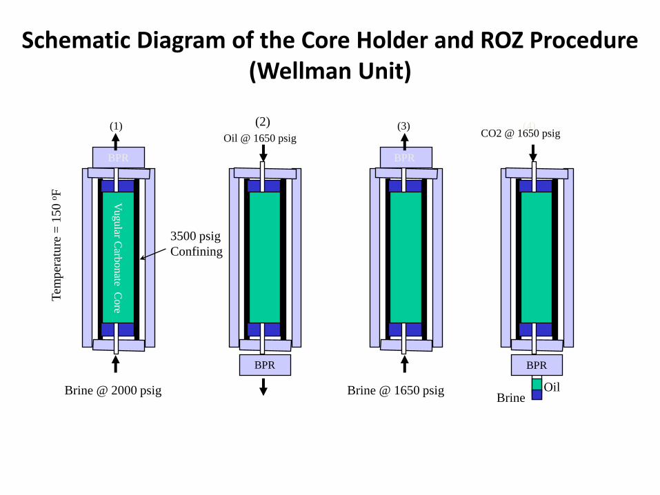
Schematic Diagram of the Core Holder and ROZ Procedure (Wellman Unit)
CO2 @ 1650 psig
BPR
Oil
3500 psig
Confining
(4) (3) (2) (1)
Tem
per
atu
re =
15
0 o
F
Oil @ 1650 psig
Brine @ 2000 psig Brine @ 1650 psig
Vugular C
arbonate C
ore
Brine
BPR
BPR BPR
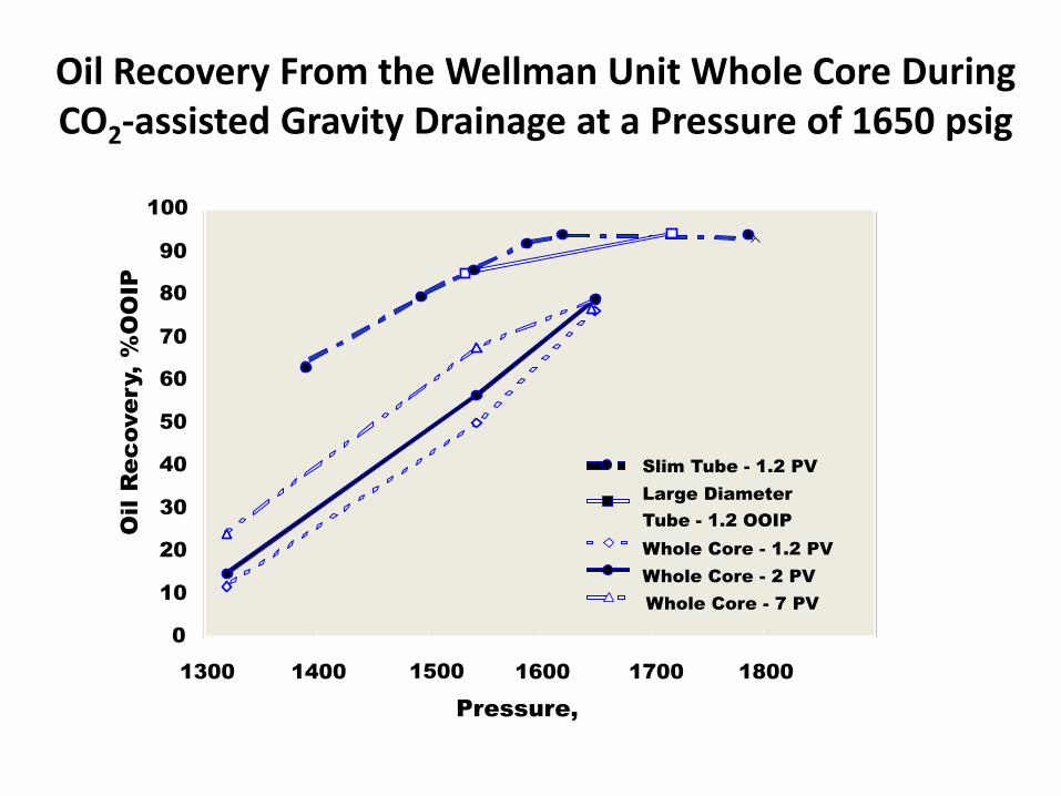
Oil Recovery From the Wellman Unit Whole Core During CO2-assisted Gravity Drainage at a Pressure of 1650 psig
1300 1400 1500 1600 1700 1800 1900
Pressure, psig
0
10
20
30
40
50
60
70
80
90
100
Oil R
ec
ove
ry, %
OO
IP
Slim Tube - 1.2 PV
Large Diameter
Tube - 1.2 OOIP
Whole Core - 1.2 PV
Whole Core - 2 PV
Whole Core - 7 PV
1500 1700
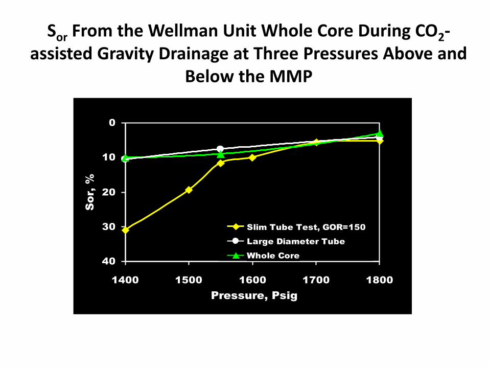
Sor From the Wellman Unit Whole Core During CO2-assisted Gravity Drainage at Three Pressures Above and
Below the MMP
0
10
20
30
40
1400 1500 1600 1700 1800
Pressure, Psig
So
r, %
Slim Tube Test, GOR=150
Large Diameter Tube
Whole Core
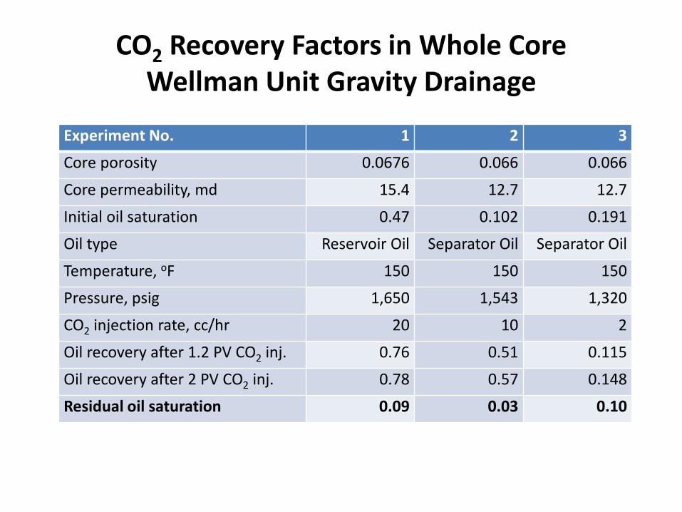
CO2 Recovery Factors in Whole Core Wellman Unit Gravity Drainage
Experiment No. 1 2 3
Core porosity 0.0676 0.066 0.066
Core permeability, md 15.4 12.7 12.7
Initial oil saturation 0.47 0.102 0.191
Oil type Reservoir Oil Separator Oil Separator Oil
Temperature, oF 150 150 150
Pressure, psig 1,650 1,543 1,320
CO2 injection rate, cc/hr 20 10 2
Oil recovery after 1.2 PV CO2 inj. 0.76 0.51 0.115
Oil recovery after 2 PV CO2 inj. 0.78 0.57 0.148
Residual oil saturation 0.09 0.03 0.10
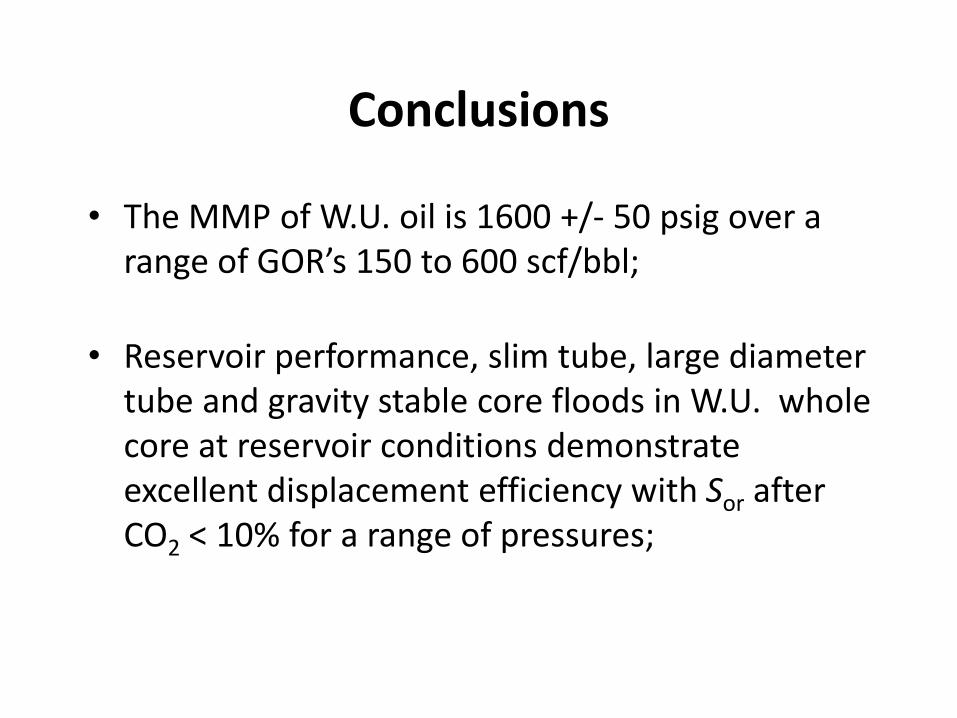
Conclusions
• The MMP of W.U. oil is 1600 +/- 50 psig over a range of GOR’s 150 to 600 scf/bbl;
• Reservoir performance, slim tube, large diameter tube and gravity stable core floods in W.U. whole core at reservoir conditions demonstrate excellent displacement efficiency with Sor after CO2 < 10% for a range of pressures;
Conclusions
• Gravity stable core flooding results from transition zone core taken from the W.U. demonstrates that oil not mobilized by water influx in the transition zone can be effectively mobilized with CO2 over a range of injection pressures;
Conclusions
• Reducing pressure from above the MMP to near the MMP does not reduce efficiency in laboratory. BHP in the W.U. could be reduced to near the MMP with no reduction in displacement efficiency. The reduction in CO2 purchases would be a positive benefit. The reduction in reservoir pressure is constrained by voidage replacement issues;
Conclusions
• CO2 flooding in the W.U. has performed exceptionally well due to gravity stable displacement above MMP. This results in excellent sweep and displacement efficiency. Over 42 bcf of CO2 has been injected and recovered 7.2 MMbbls of tertiary oil. The resulting utilization is 5.83 Mcf CO2 injected per barrel of incremental oil as of the late 90’s

Enhanced Oil Recovery in ULR CO2 Injection
CO2 Oil Recovery
Objective
To observe the effect of CO2 into ULR core and the effect that it may have on oil productivity.
CO2 Oil Recovery Motivation
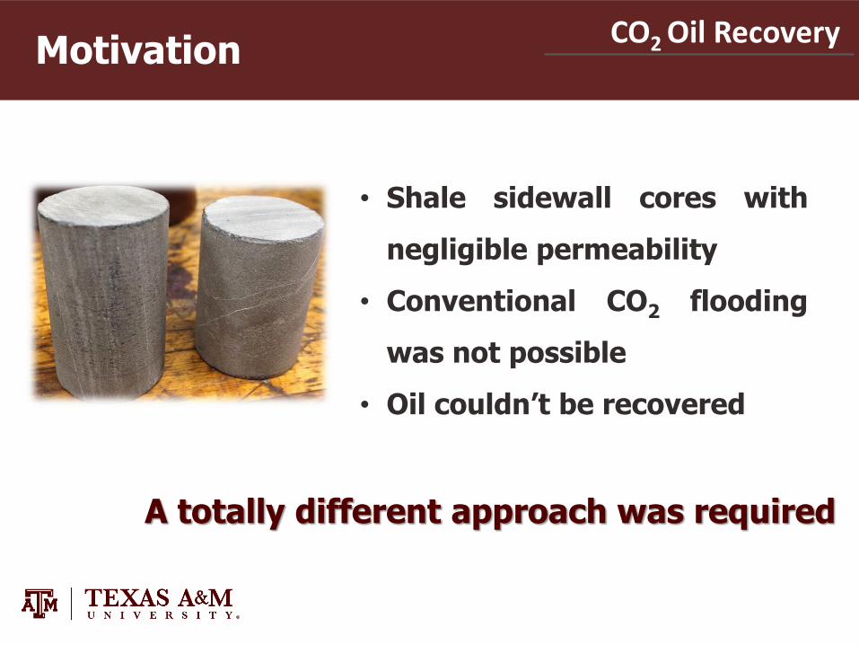
• Shale sidewall cores with
negligible permeability
• Conventional CO2 flooding
was not possible
• Oil couldn’t be recovered
A totally different approach was required
CO2 Oil Recovery
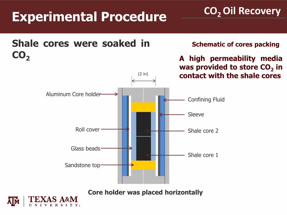
Shale cores were soaked in CO2
(2 in)
Aluminum Core holder Confining Fluid
Sleeve
Roll cover Shale core 2
Glass beads Shale core 1
Sandstone top
Core holder was placed horizontally
Experimental Procedure
A high permeability media was provided to store CO2 in contact with the shale cores
Schematic of cores packing
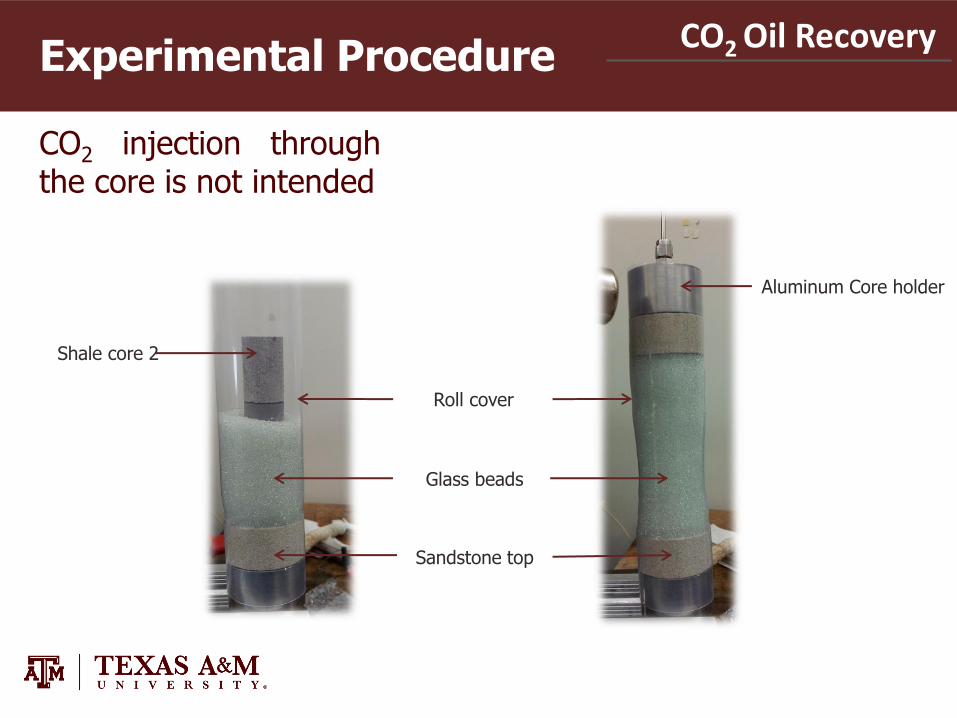
CO2 Oil Recovery Experimental Procedure
Aluminum Core holder
Glass beads
Sandstone top
Roll cover
Shale core 2
CO2 injection through the core is not intended
CO2 Oil Recovery
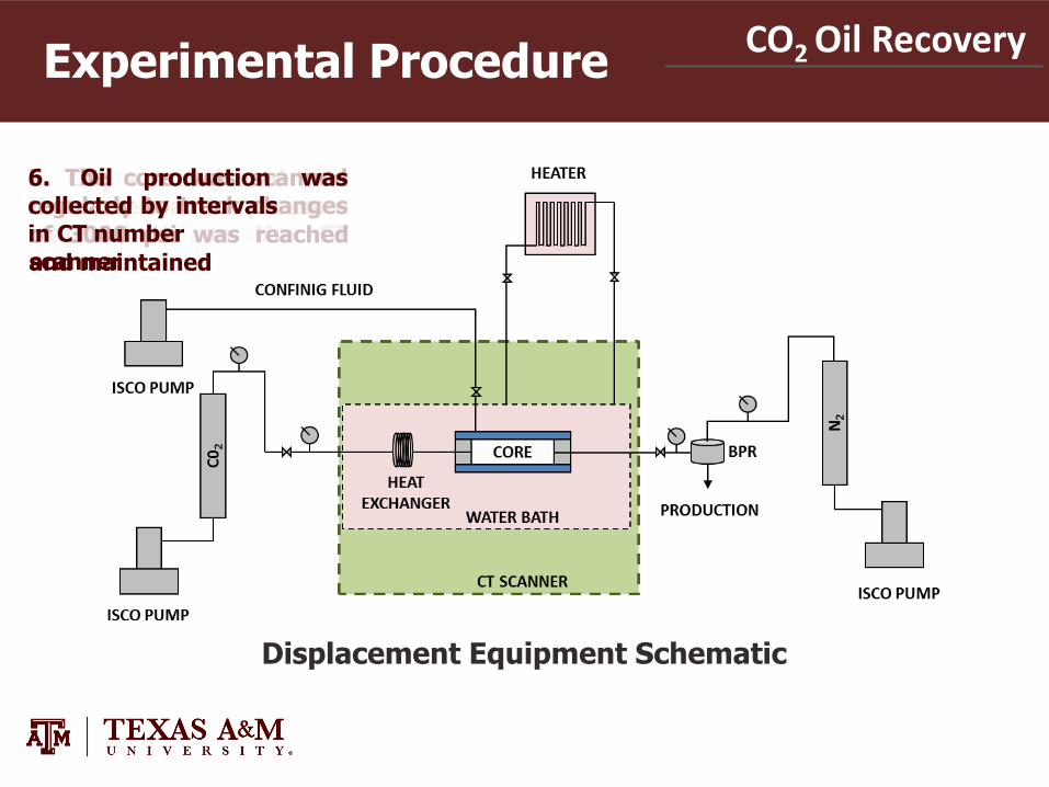
Displacement Equipment Schematic
Experimental Procedure
1. Cores were packed, and a confining pressure of 250 psi was applied
2. The core holder was placed inside a circulating water bath on the CT scanner
3. Temperature was increased to 150 F 4. CO2 was injected into the system and a pressure of 3000 psi was reached and maintained
5. The core was scanned regularly to track changes in CT number
6. Oil production was collected by intervals

CO2 Oil Recovery Experimental Equipment

New CT Scanner at Texas A&M
PE Department
CO2 Oil Recovery
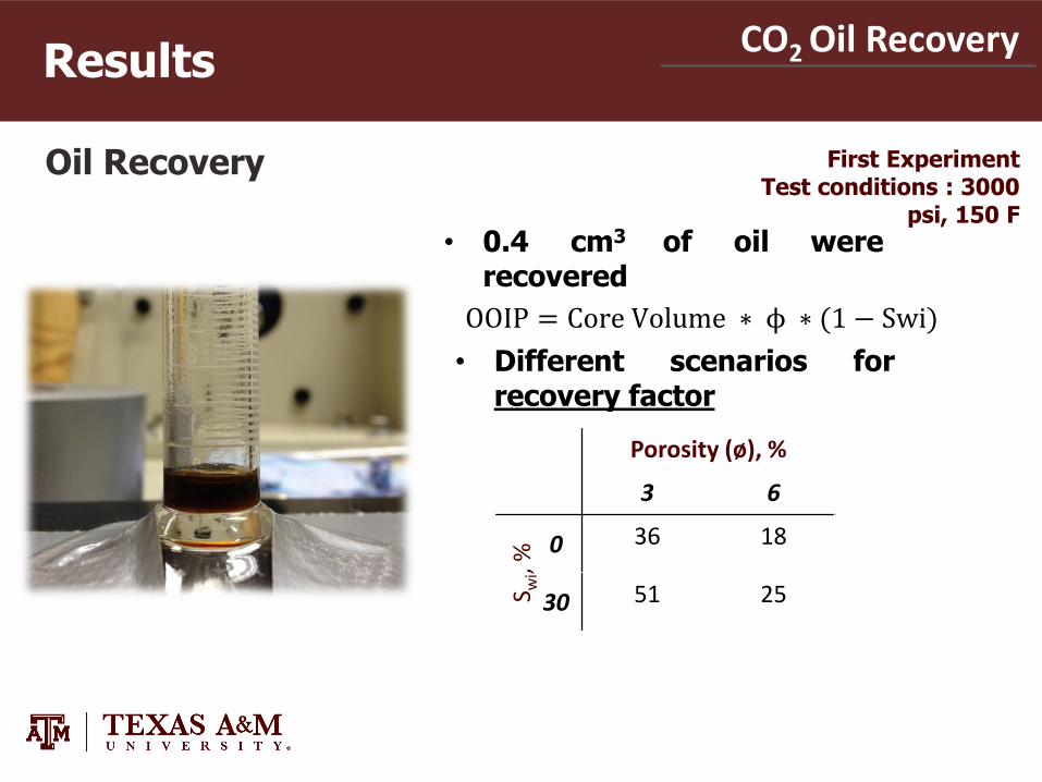
• 0.4 cm3 of oil were recovered
Results
First Experiment Test conditions : 3000
psi, 150 F
Oil Recovery
OOIP = Core Volume ∗ ϕ ∗ (1 − Swi)
Porosity (ø), %
3 6 S w
i, %
0 36 18
30 51 25
• Different scenarios for recovery factor
CO2 Oil Recovery Results
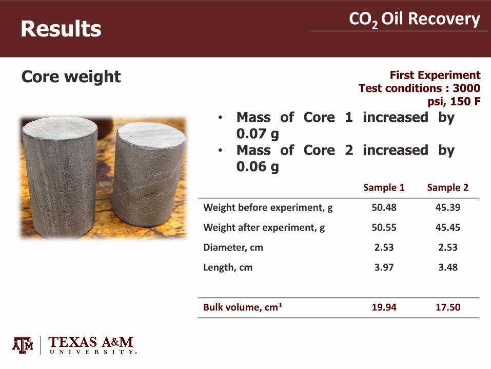
Core weight
• Mass of Core 1 increased by 0.07 g
• Mass of Core 2 increased by 0.06 g
Sample 1 Sample 2
Weight before experiment, g 50.48 45.39
Weight after experiment, g 50.55 45.45
Diameter, cm 2.53 2.53
Length, cm 3.97 3.48
Bulk volume, cm3 19.94 17.50
First Experiment Test conditions : 3000
psi, 150 F
CO2 Oil Recovery Results
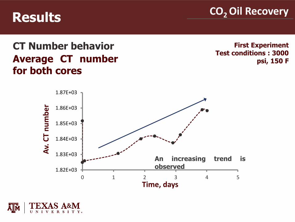
CT Number behavior
1.82E+03
1.83E+03
1.84E+03
1.85E+03
1.86E+03
1.87E+03
0 1 2 3 4 5
Av.
CT
nu
mb
er
Time, days
Average CT number for both cores
An increasing trend is observed
First Experiment Test conditions : 3000
psi, 150 F
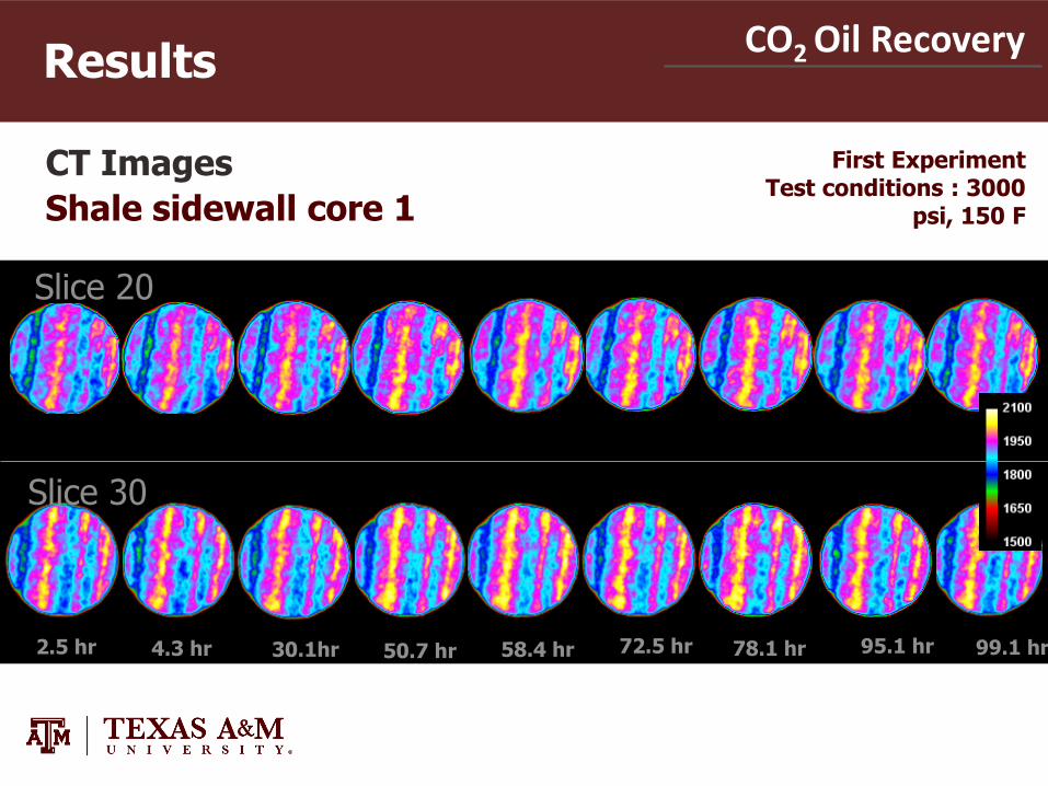
CO2 Oil Recovery Results
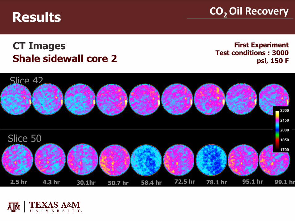
CT Images
Shale sidewall core 1
Slice 20
Slice 30
2.5 hr 4.3 hr 30.1hr 50.7 hr 58.4 hr 72.5 hr 78.1 hr 95.1 hr 99.1 hr
First Experiment Test conditions : 3000
psi, 150 F
CO2 Oil Recovery Results
CT Images
Shale sidewall core 2
Slice 42
Slice 50
2.5 hr 4.3 hr 30.1hr 50.7 hr 58.4 hr 72.5 hr 78.1 hr 95.1 hr 99.1 hr
First Experiment Test conditions : 3000
psi, 150 F
CO2 Oil Recovery
Since CT number correlates to density
Results
0
10
20
30
40
50
60
0 1000 2000 3000 4000 5000 6000
Den
sity
, lb
/ft3
Pressure, psia
Vapor CO2Supercritical CO2heptanehexanePentaneButane
2
T = 150 °F
1
The experiment was repeated at 1600 psi, where a higher density difference exists

CO2 Oil Recovery
• 0.4 cm3 of oil were recovered
Results
Oil Recovery
OOIP = Core Volume ∗ ϕ ∗ (1 − Swi)
Porosity (ø), %
3 6 S w
i, %
0 39 19
30 55 28
• Different scenarios for recovery factor
This test was prematurely terminated because of a water leak
Second Experiment Test conditions : 1600
psi, 150 F

CO2 Oil Recovery Results
Core weight
• Mass of Core 1 increased by 0.95 g
• Mass of Core 2 increased by 0.86 g
Sample 1 Sample 2
Weight before experiment, g 40.09 36.04
Weight after experiment, g 41.04 36.90
Diameter, cm 2.53 2.52
Length, cm 3.62 3.29
Bulk volume, cm3 18.20 16.42
Second Experiment Test conditions : 1600
psi, 150 F

CO2 Oil Recovery
1.50E+03
1.51E+03
1.51E+03
1.52E+03
1.52E+03
1.53E+03
1.53E+03
1.54E+03
0 20 40 60 80
Av.
CT
nu
mb
er
Time, hours
Results
CT Number behavior
Average CT number for sidewall core 1
A decreasing trend is observed
Second Experiment Test conditions : 1600
psi, 150 F
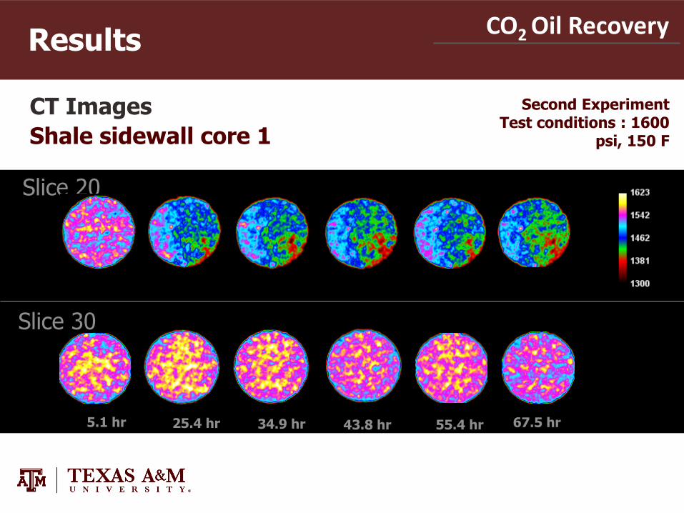
CO2 Oil Recovery Results
CT Images
Shale sidewall core 1
Slice 20
Slice 30
5.1 hr 25.4 hr 34.9 hr 43.8 hr 55.4 hr 67.5 hr
Second Experiment Test conditions : 1600
psi, 150 F

CO2 Oil Recovery Results with CT Number
Average CT number for sidewall core 2
Different trends are observed
Second Experiment Test conditions : 1600
psi, 150 F
1.36E+03
1.40E+03
1.44E+03
1.48E+03
1.52E+03
1.56E+03
0 20 40 60 80
Av
CT
nu
mb
er
Time, days
Slice 1
1.54E+03
1.54E+03
1.55E+03
1.55E+03
1.56E+03
0 20 40 60 80
Av
CT
nu
mb
er
Time, days
Slice 10
1.48E+03
1.50E+03
1.52E+03
1.54E+03
1.56E+03
0 20 40 60 80
Av
CT
nu
mb
er
Time, days
Slice11
1.36E+03
1.40E+03
1.44E+03
1.48E+03
1.52E+03
0 20 40 60 80
Av
CT
nu
mb
er
Time, days
Slice 15
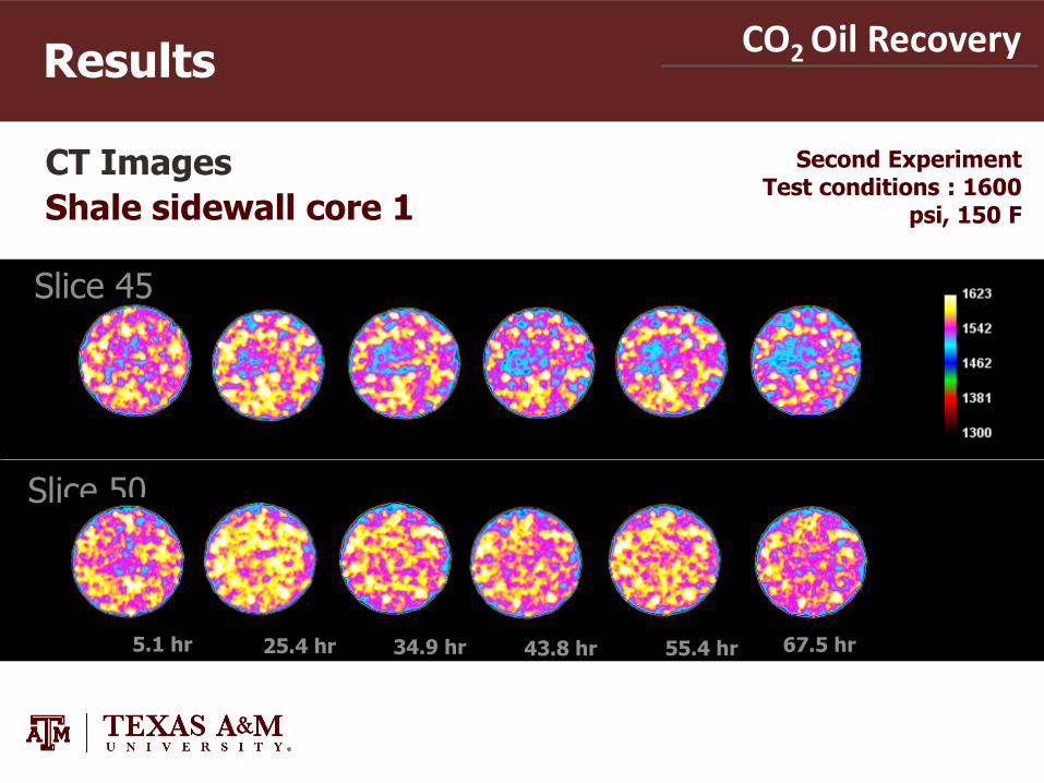
CO2 Oil Recovery Results
CT Images
Shale sidewall core 1
Slice 45
Slice 50
5.1 hr 25.4 hr 34.9 hr 43.8 hr 55.4 hr 67.5 hr
Second Experiment Test conditions : 1600
psi, 150 F
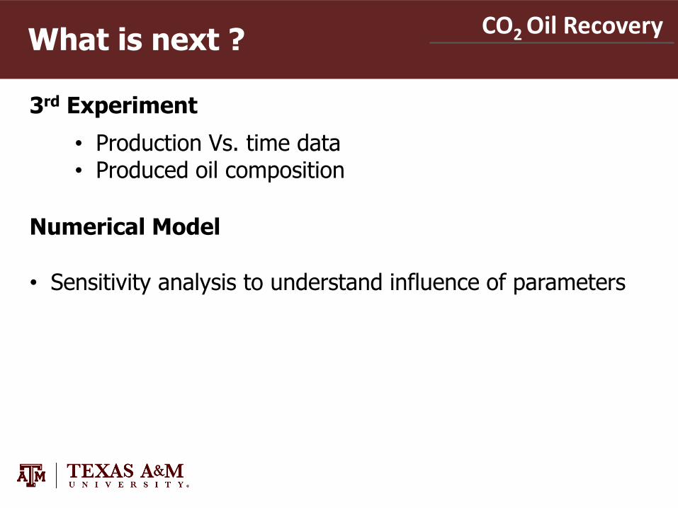
CO2 Oil Recovery What is next ?
3rd Experiment
• Production Vs. time data • Produced oil composition
Numerical Model
• Sensitivity analysis to understand influence of parameters

CO2 Oil Recovery
• Oil production was accomplished by soaking shale cores with CO2 at 3000 psi and 1600 psi. Recovery in both cases is estimated to be from 18 to 55 % of OOIP. The permeability of the cores does not allow for conventional CO2 flooding.
• CT imaging was done during the course of the experiment
revealing changes inside the sidewall cores.
• Changing the pressure of the test influenced the behavior of CT number, this could be related to the different densities of CO2 at the two experimental conditions.
• More work is required to better understand the mechanisms causing oil production during these tests.
Conclusions
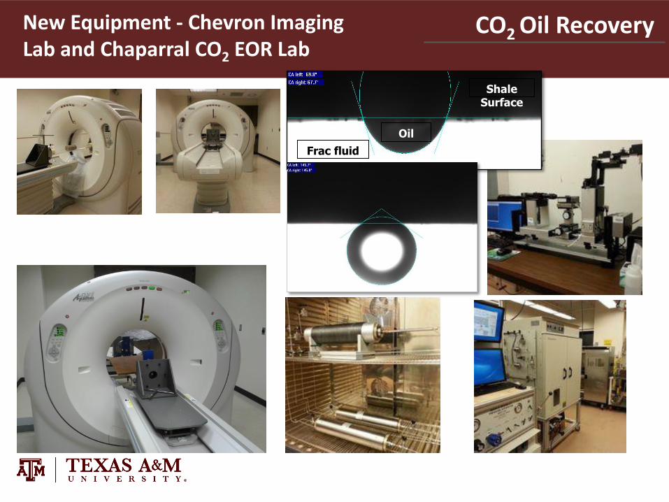
CO2 Oil Recovery New Equipment - Chevron Imaging Lab and Chaparral CO2 EOR Lab
Frac fluid
Oil
Shale Surface

CO2 and Enhanced Oil Recovery in Unconventional Liquid Reservoirs
Department of Petroleum Engineering
Texas A&M University
Dr. David Schechter
Please Join Our Newly
Established JIP

Dimensionless Curves Improving Prediction of CO2 Injection in Conventional Reservoirs

• Cumulative dimensionless WF
calculated for each pattern
Methodology Evaluation of Water-Flood Recovery
Primary Production DCA Sample: Pattern J-1 (8.5%/yr)
Primary Production DCA Sample: Pattern J-7 (9%/yr)
WF recovery = incremental production (over primary)
Anino Adokpaye 2013

Methodology Dimensionless Recovery Curves – WF & CO2 Comparisons
While a pattern is under the initial pure CO2 slug (prior to WAG), DTI = DCI
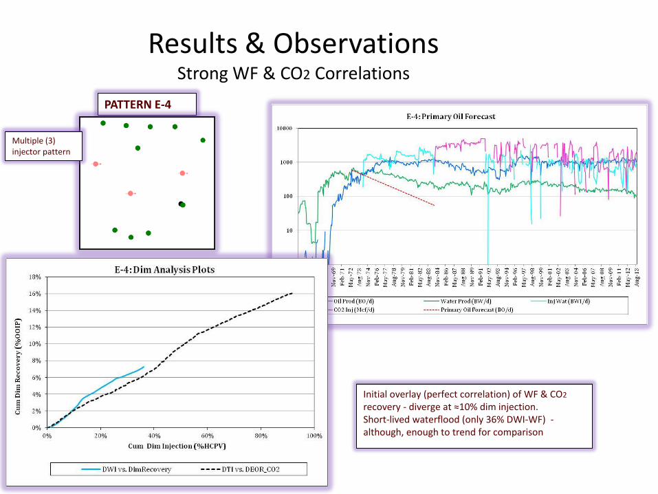
Results & Observations Strong WF & CO2 Correlations
Initial overlay (perfect correlation) of WF & CO2 recovery - diverge at ≈10% dim injection. Short-lived waterflood (only 36% DWI-WF) - although, enough to trend for comparison
PATTERN E-4
Multiple (3) injector pattern

Results & Observations Strong WF & CO2 Correlations
PATTERN J-5
WF & CO2 recovery curves remain parallel through 200% dimensionless injection!
Curves tend to diverge at ≈20% DEOR
CO2 Oil Recovery
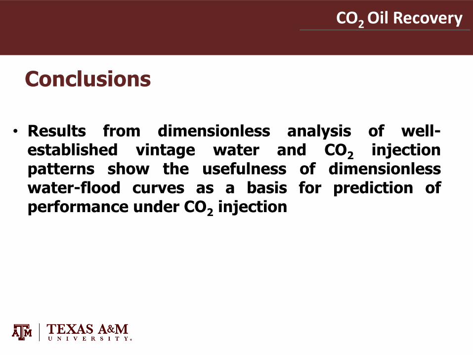
Conclusions
• Results from dimensionless analysis of well-established vintage water and CO2 injection patterns show the usefulness of dimensionless water-flood curves as a basis for prediction of performance under CO2 injection
Surfactant Studies in ULR CO2 Injection in Conventional and Unconventional Liquid Reservoirs
Department of Petroleum Engineering
Texas A&M University
Dr. David Schechter

Barnett Shale The penetration of anionic surfactant in this particular siliceous shale core is shown in this sequence of fluid in seven cross sectional views of the core before flooding, 0 hours, 30 minutes, 1 hour, 2 hours, 4 hours and 20 hours after flooding. This slice is one of the 18 slices used to create the horizontal view in the previous slice
Fracture
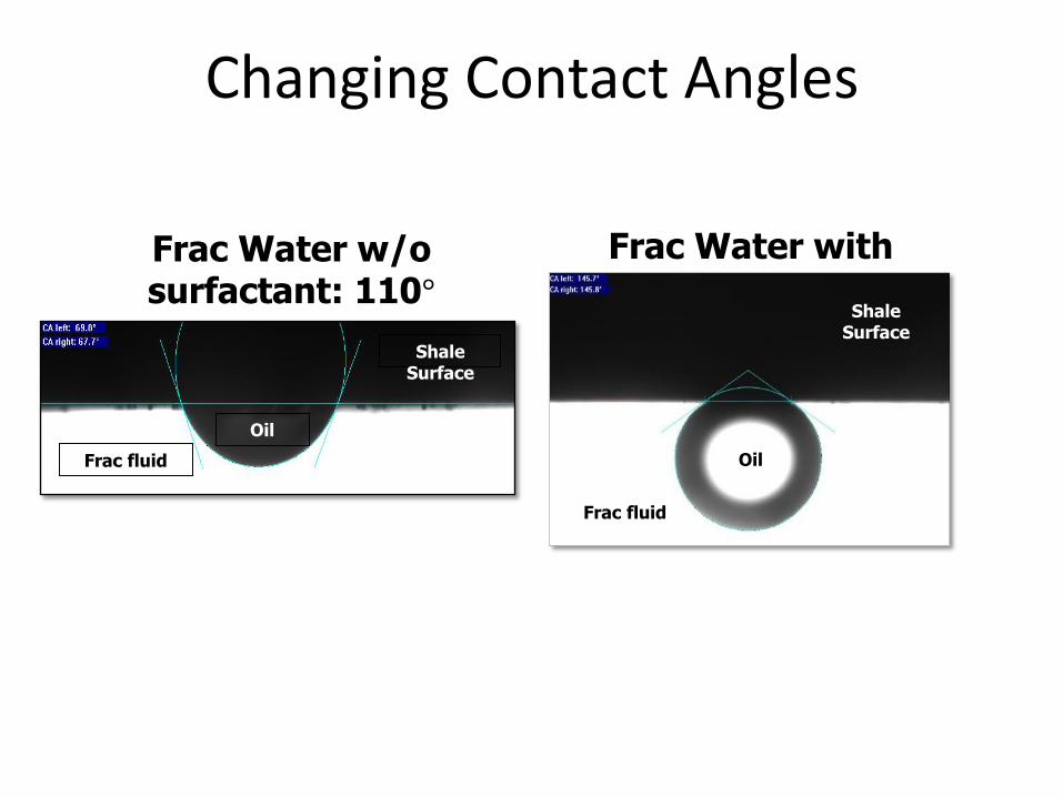
Changing Contact Angles
Frac Water w/o surfactant: 110°
Frac Water with surfactant: 35°
Frac fluid
Oil
Shale Surface
Oil
Shale Surface
Frac fluid
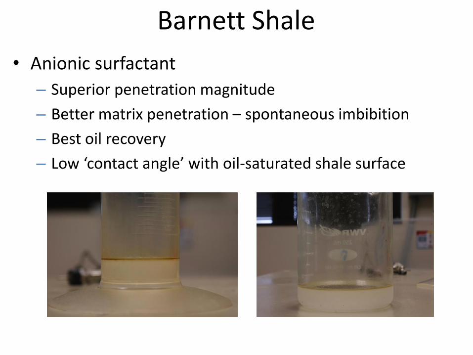
Barnett Shale
• Anionic surfactant
– Superior penetration magnitude
– Better matrix penetration – spontaneous imbibition
– Best oil recovery
– Low ‘contact angle’ with oil-saturated shale surface
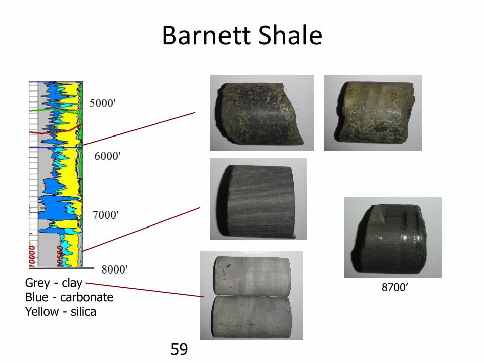
Barnett Shale
59
Grey - clay Blue - carbonate Yellow - silica
8700’

Contact Angle & IFT Measuring Capabilities
• Static and dynamic contact angles
• Surface and interfacial tension
• Surface free energy of solids and their components
• Temperature control unit to maintain reservoir temperature
Dataphysics OCA 15 Pro
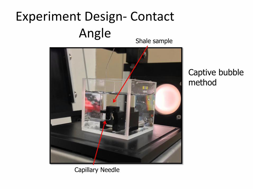
Experiment Design- Contact Angle
Shale sample
Capillary Needle
Captive bubble method