NASA Technical Paper 2797

1988

National Aeronautics and Space Administration

Scientific and Technical .Information Division

A Simplified Approach to Axisymmetric Dual-Reflector Antenna Design

Raymond L. Barger Langley Research Center Hampton, Virginia

https://ntrs.nasa.gov/search.jsp?R=19880007279 2018-06-15T16:26:48+00:00Z

Summary A procedure is described for designing dual-

reflector antennas. The analysis is developed by tak- ing each reflector to be the envelope of its tangent planes. The slopes of the emitted rays are speci- fied rather than the phase distribution in the emit- ted beam. Thus, both the output wave shape and the angular distribution of intensity can be specified.

Computed examples include variations from both Cassegrain and Gregorian systems. These examples include deviation from uniform source distributions and from the parallel-beam property of conventional sys tems.

Introduction In theory it is possible to specify, within lim-

its, both the emitted amplitude distribution and the phase distribution of a dual-reflector system when both surfaces are properly shaped. The problem of determining these shapes has been treated in refer- ences 1 and 2 with a combination of differential and algebraic equations. This system of equations tends to be unwieldy, and consequently in both references the method of solution is only indicated, with the specific formulas omitted.

Although the present approach is an approximate procedure, it can, in theory, be made as accurate as desired by taking sufficiently small step sizes. The simplifying concept is to treat each of the two reflectors as the envelope of its tangent planes. This technique permits the mathematical problem to be reduced to one of solving a set of nonlinear algebraic equations.

Computed examples include both modified Cassegrain and modified Gregorian systems. Inas- much as the emphasis in the present analysis is on simplicity of concept, only axisymmetric systems are treated. It should be noted that if the reflector sys- tem utilizes only a segment (e.g., a quadrant) of the axisymmetric design, then a cross polarization exists in the output beam since the antenna normally does not emit a circularly polarized wave.

I

t

I

I Symbols I b exponent of cos 80

E beam energy

I intensity

m slope of ray relative to system centerline

coordinates, x taken along system centerline and y in radial direction

(XI, Yl), (X2, Y2) midpoint of straight seg- ment tangent to reflector meridian line

x3, y3

(XI, yl), (22, y2)

point at which ray intersects reference plane

initial point of straight segment tangent to reflector , meridian line ,

8 angle ray makes with system centerline

Subscripts:

0

1

2

3

b

C

origin or ray emanating from origin

tangent segment of subreflector

tangent segment of main reflector

vertical plane along which output intensity is specified

ray reflected from main .reflector

ray reflected from subreflec- tor to main reflector ,

i index I

min, max, total minimum, maximum, and total

Analysis

Reflector and Ray Geometry I As was mentioned in the Introduction, each

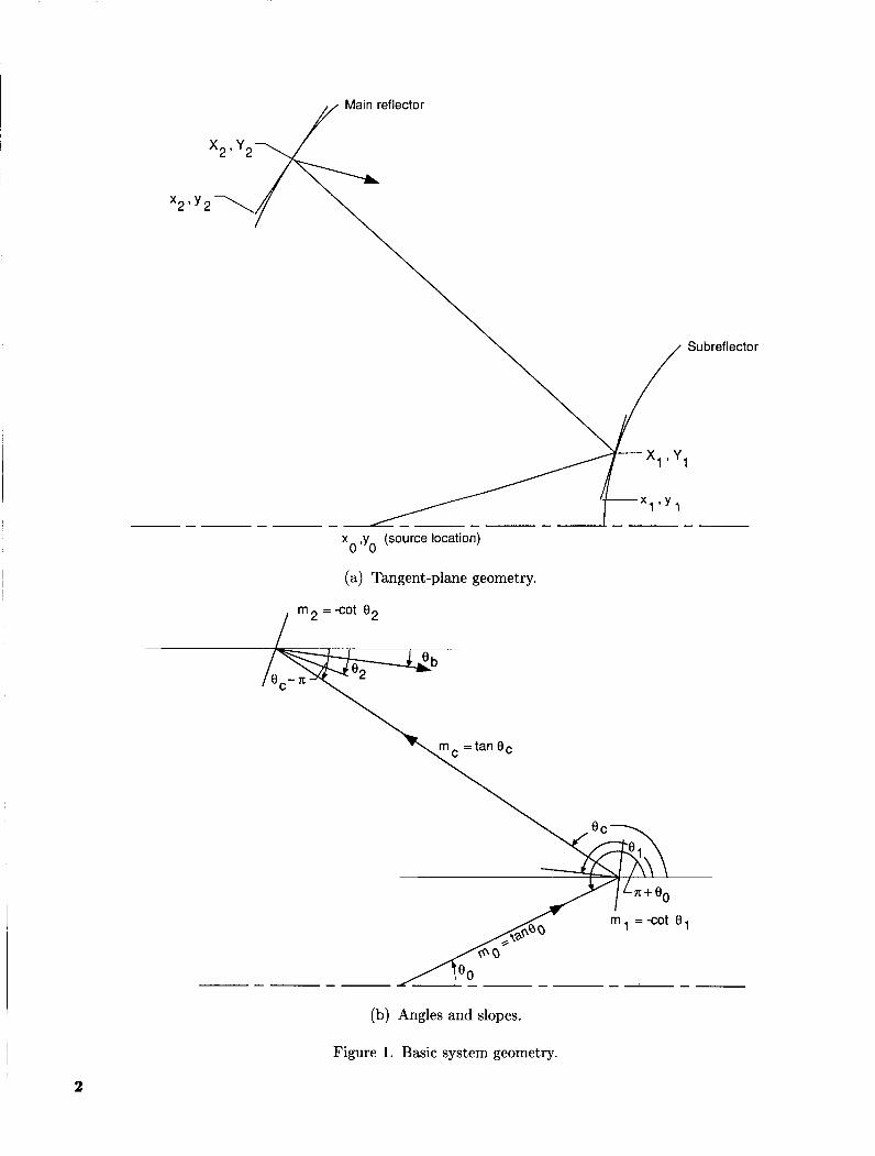
curved reflector surface is treated as the envelope of its tangent planes. Since each of these surfaces is axisymmetric, it can be specified by the meridian line cut by a vertical plane. Then the tangent plane along this meridian appears simply as a straight line segment. (See fig. l(a).)

The geometry for tracing a ray through the sys- tem is shown in figure l(b). The reflection condition at the subreflector gives

R .*2 mz-1

Main reflector

x 2 ' y 2 \

Su breflector

x y (source location) 0 ' 0

(a) Tangent-plane geometry.

m 2 = -cot e2

I

\mc =tan ec

(b) Angles and slopes.

Figure 1. Basic system geometry.

2

To find the relation between the slopes, we take the tangent of both sides:

(2) - tan Oc + tan 80

1 - tan8, tan80 -

2 tan 81 1 - tan281

tan281 =

Similarly, at the second reflector,

tan(282) = tan[& + (8, - T ) ] (3)

or

(4) - tan 83 + tan 8,

1 - tan83 tan8, - 2 tan 62

1 - tan282 Since the slope of the local tangent to the reflector is the negative reciprocal of the slope of its normal (ml = -cot el), equation (2) yields

-2m1 - rno+m, m 7 - 1 l-mornc (5) --

and, similarly, equation (4) yields

(6) -2m2 - m3+mc mg-1 1-m3rnC --

Referring to figure l(a), if we denote the coordi- nates of the initial point of a subreflector segment by (21, y1) and denote the reflection points by capital letters (XI, Yl), then the reflection point is specified to be at the midpoint of the segment simply by tak- ing the segment length to be twice the distance from (21, y1) to (X1,Yl). The main reflector is treated similarly. The slopes and point coordinates are re- lated linearly as follows:

y 2 - Yl x2 - x1 m, =

Yl -Yo x1- 20

mo =

y1- Y 1

x1- 21 ml =

y2 - Y2

x2 - 2 2 m2 =

(7)

(9)

The intensity distributions are determined as fol- lows. The intensity distribution to be assigned ar- bitrarily as the output of the system is most conve- niently specified along a vertical plane, usually taken near the aperture plane. Thus, if the output inten- sity distribution I(Y3) is assigned as a function of Y3 along a vertical plane taken at X3, then the ray that intersects this plane at Y3 is related to the ini- tial source emission angle 80 through the energy rela- tion, which is given in the next section. Furthermore,

it is appropriate, with the present method, to spec- ify the ray slope distribution of the system output beam rather than the phase distribution. Thus (see fig. 2(a)), in the equation for the ray reflected from (X2, Y2) through (X3, Y3),

and X3, Y3, and mb are all known quantities.

Energy Relation The value of Y3 is determined from the energy

relation as follows. The intensity distribution Io(80) emitted by the source antenna is (see fig. 2(b))

and consequently all the energy emitted within this segment is

and the relative amount of energy emitted is

(13) Eo (80) Eo (80)

EO (00,max) Etotd -

where denotes the edge of that part of the source beam that is to be utilized.

The intensity of the output beam is specified as a function of Y3 along the vertical plane at X3. Thus, the energy emitted through the annulus at Y3 with width dY3 is (see fig. 2(a))

The energy emitted through the ring at Y3 is

where the ray through Y3,min is that emitted at 8 0 , ~ i ~ by the source. The relative energy is

Comparing equation (15) with equation (13) enables one to determine the Y3 corresponding to a given 80. As a rule, the prescribed intensity distribution 13(y) in equation (14) is taken as a relatively simple an- alytic expression. Consequently, the energy integral

3

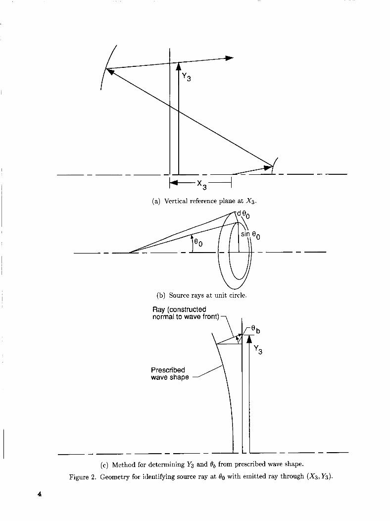
(a) Vertical reference plane at X3.

(b) Source rays at unit circle.

Ray (constructed normal to wave front) 7

(c) Method for determining Y3 and 8b from prescribed wave shape.

Figure 2. Geometry for identifying source ray at 80 with emitted ray through (X3, Y3).

4

in equation (14) can be evaluated in closed form and E(Y3) is determined in analytic form. Furthermore, the source intensity distribution Io(6') can often be described as some power of cos 6' or as a linear com- bination of such functions, so that E(6'o) can be de- termined in analytic form from equation (12).

Before proceeding to the solution of the equations for the reflector surfaces, we may pursue further the significance of the form of the system performance specification. Although for some problems it is appropriate to specify the intensity and beam direction distributions along some vertical plane, it is important to observe that these distributions can be obtained by specifying the more fundamental quan- tities of output wave shape and the intensity dis- tribution as a function of ray direction. Thus, in reference to figure 2(c), the wave shape and the rela- tive energy as a function o f & are prescribed. Since the wave shape is known, normals to the wave shape can be constructed and their intersections with the vertical plane at X3 determined. These normals, which represent rays, have slope mb = tan&. Thus, with E(&) prescribed, these intersections determine E(Y3). Consequently, both mb and Y3 are deter- mined for each ray of the output beam.

Solution of Equations

To determine the reflector shapes, the set of seven equations (5) to (11) are to be solved for the unknown quantities X I , Y1, X2, Y2, ml , ma, and m,. The ap- proach taken here is to eliminate all unknowns except ma, solve the resulting (highly nonlinear) equation for m2 numerically, and then substitute back into the other equations to determine the remaining un- knowns. The details of this procedure follow.

Define -2m2

R(m2) = 7 m2 - 1

and substitute R into equation ( 6 ) , which (noting that m3 = mb) can then be written as

(1 - mbm,)R(m2) = mb + m,

and solved for m, to obtain

Equations (10) and (11) are each solved for Y2, and then Y2 is eliminated by equating the resulting expressions:

This equation is solved for X2 to yield

This expression may be substituted back into equa- tion (11) to obtain an expression for Y2 as a function of mg only:

Eliminating Y1 between equations (7) and (8) yields

which can be solved for X I and expressed as a func- tion of m2 with substitutions from equations (17), (18), and (19):

(20) This result is substituted back into equation (8) to obtain

Equation (9) now becomes

Substituting from equations (17) and (22) into equa- tion ( 5 ) yields

This equation is solved numerically by a forward seeker algorithm that finds the zeros of the function on the left side of equation (23). Once the root is found, we can find the remaining quantities by re- peating the above substitutions with the known value of ma. Thus, m, is obtained from equation (17), and X2, Y2, X i , and Y1 are obtained from equations (18)

To determine the next pair of points on the two reflectors, 6'0 is incremented. Then 51, y1, z2, and y2 are incremented by specifying ( X I , Y1) to be the midpoint of a segment on the subreflector and sim- ilarly for (X2,Y2) on the main reflector. Thus, for example,

to (21).

5

The procedure can then be repeated for the new value of 00. Inasmuch as equation (23) is highly nonlinear and possesses multiple roots, some care must be exercised in setting the limits of the range of m 2 over which the numerical algorithm seeks a solution. Fortunately, the limits are known to a close approximation because specifying even sizeable variations from a uniform intensity distribution or from a parallel-ray output beam does not result in large geometry variations from a conventional Cassegrain or Gregorian system.

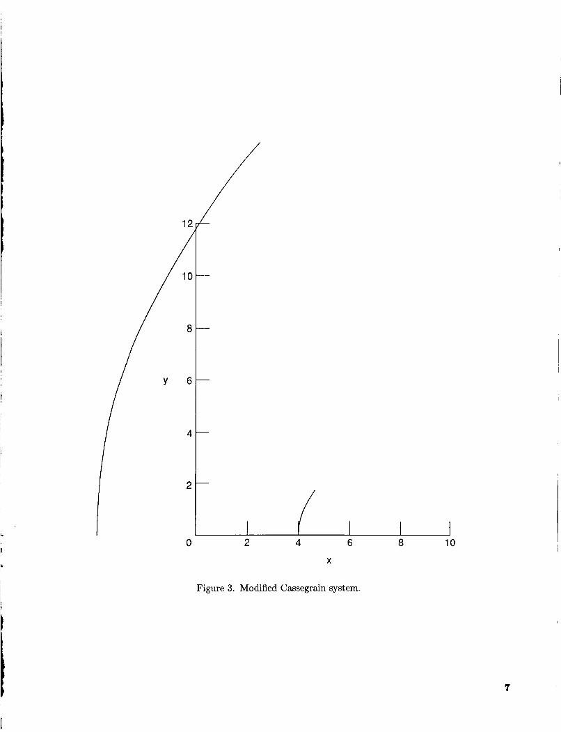
Computed Examples Figure 3 shows a modified Cassegrain system for

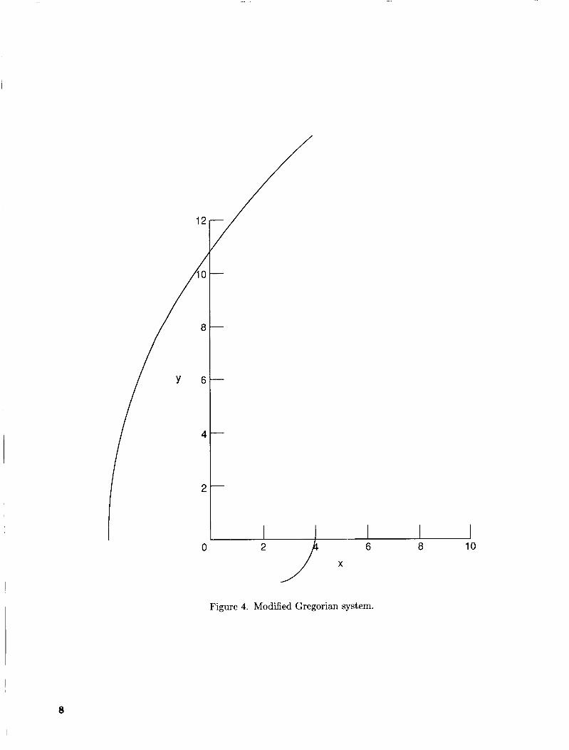
which the source distribution varies as cos8 00 but the emitted beam is specified to have a uniform distribution. Figure 4 gives a similarly designed modification of a Gregorian system.

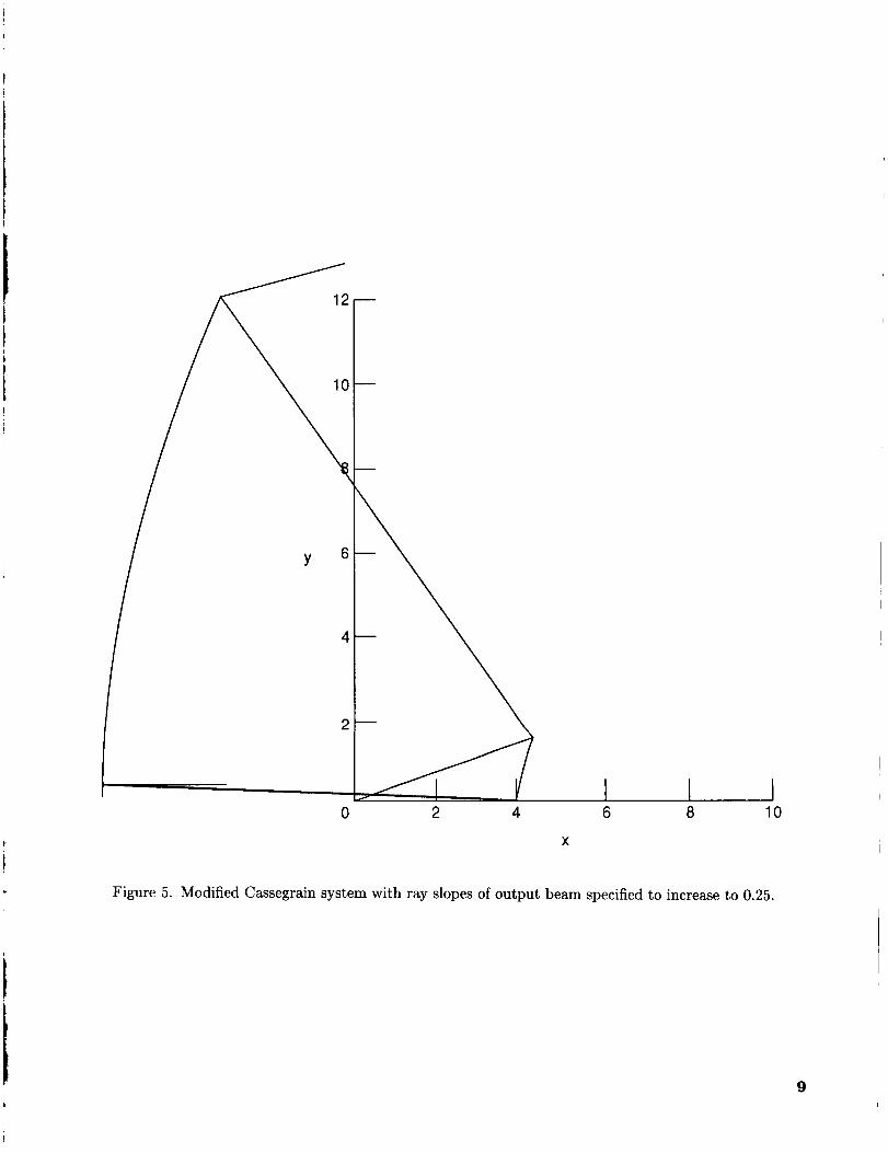
Figure 5 shows a modified Cassegrain system for which the slopes of the rays of the output beam are specified to increase gradually up to a value of 0.25:

2

mg = 0.25 (") Y3,rnax

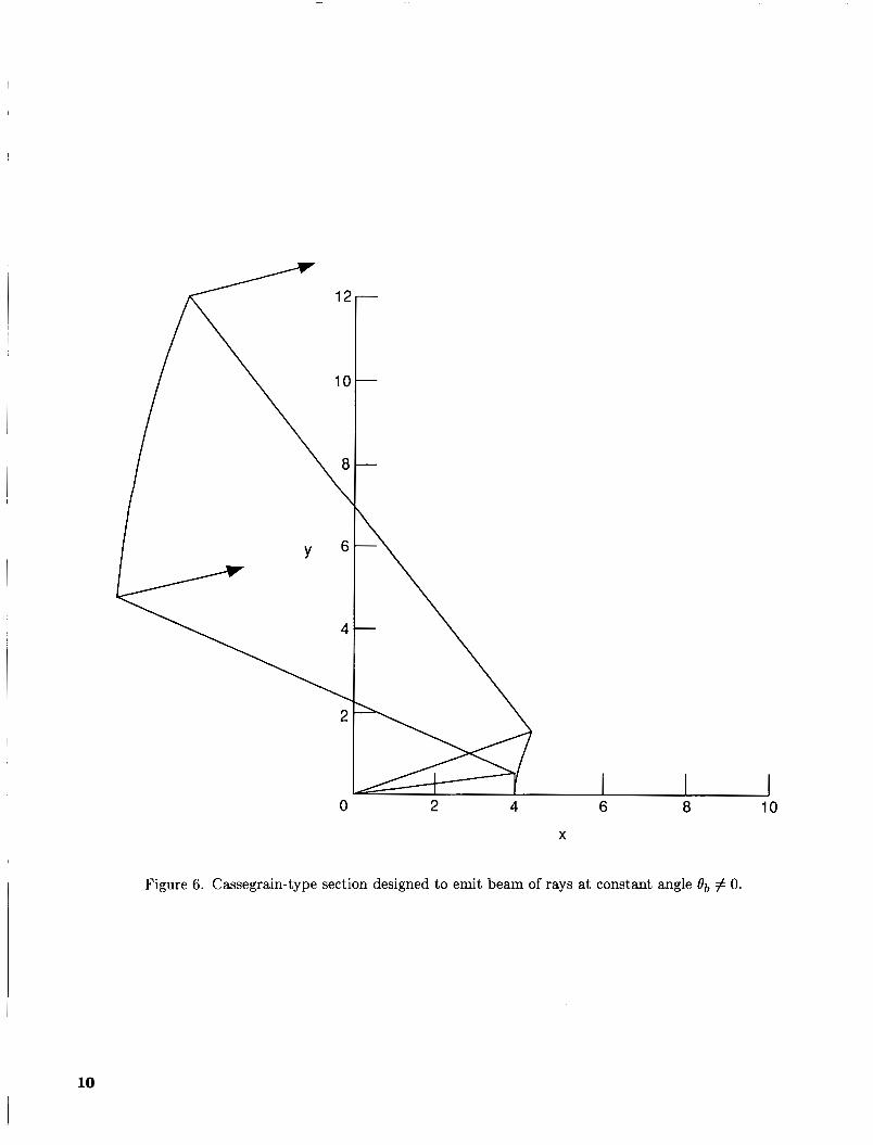
Figure 6 shows an offset system consisting of seg- ments of a subreflector and a main reflector designed so that the emitted rays all have a slope of 0.25 rel- ative to the system centerline. In such a system, the

cross-polarization phenomenon mentioned in the In- troduction would exist.

Concluding Remarks A procedure has been described for designing

dual-reflector antennas. The analysis was developed by taking each reflector to be the envelope of its tangent planes, so that the reflection condition is satisfied on each of these planes. The slopes of the emitted rays were specified rather than the phase distribution in the emitted beam.

Computed examples included variations from both Cassegrain and Gregorian systems. These ex- amples include deviation from uniform source distri- bution and from the parallel-beam property of con- ventional systems.

NASA Langley Research Center Hampton, VA 23665-5225 February 2, 1988

References 1. Galindo, Victor: Design of Dual-Reflector Antennas

With Arbitrary Phase and Amplitude Distributions. IEEE Trans. Antennas d Propag., vol. 12, no. 4, July

2. Kinber, B. Ye.: On Two-Reflector Antennas. Radio Eng. d Electron. Phys., no. 6, June 1962, pp. 914-921.

1964, pp. 403-408.

6

12

Y

10

8

6

4

2

0 2 4 6 8 10

X

Figure 3. Modified Cassegrain system.

7

12

/” 8

6

4

2

8

I

6 Y

4

2

0 2 4 6 a 10

X

Figure 5. Modified Cassegrain system with ray slopes of output beam specified to increase to 0.25.

9

2 4 6 8 10

X

Figure 6. Cassegrain-type section designed to emit beam of rays at constant angle O b # 0.

10

I

Iw\sA National Aeronautics and Report Documentation Page

1. Report No. NASA TP-2797

2. Government Accession No.

1. Title and Subtitle A Simplified Approach to Axisyrnmetric Dual-Reflector Antenna Design

19. Security Classif.(of this report) 20. Security Classif.(of this page) Unclassified Unclassified

7. Author(s) Raymond L. Barger

21. No. of Pages 22. Price 11 A02

3. Performing Organization Name and Address NASA Langley Research Center Hampton, VA 23665-5225

12. Sponsoring Agency Name and Address National Aeronautics and Space Administration Washington, DC 20546-0001

15. Supplementary Notes

3. Recipient’s Catalog No.

5 . Report Date

March 1988 6. Performing Organization Code

8. Performing Organization Report No.

L- 16392 10. Work Unit No.

505-61-71-04 11. Contract or Grant No.

13. Type of Report and Period Covered

Technical Paper 14. Sponsoring Agency Code

16. Abstract A procedure is described for designing dual-reflector antennas. The analysis is developed by taking each reflector to be the envelope of its tangent planes. The slopes of the emitted rays were specified rather than the phase distribution in the emitted beam. Thus, both the output wave shape and the angular distribution of intensity can be specified. Computed examples include variations from both Cassegrain and Gregorian systems. These examples include deviation from uniform source distributions and from the parallel-beam property of conventional systems.

17. Key Words (Suggested by Authors(s)) Dual-reflector antennas

18. Distribution Statement Unclassified-Unlimited

lASA FORM 1626 OCT 86 NASA-Langley, 1988

For sale by the National Technical Information Service, Springfield, Virginia 22161-2171