simple linear regression - musc
TRANSCRIPT
Simple linear regression
Biometry 755
Spring 2008
Simple linear regression – p. 1/40
Overview of regression analysis
• Evaluate relationship between one or more independentvariables (X1, . . . , Xk) and a single continuous dependentvariable (Y ).
• Terminology: “Regress Y on X”
• Example Relationship between risk of nosocomialinfection (dependent variable, Y ) and routine culturingratio (independent variable, X)
0 10 20 30 40 50 60
23
45
67
8
Routine culturing ratio
Pro
babi
lity
of n
osoc
omia
l inf
ectio
n x
100
Simple linear regression – p. 2/40

Goals of a regression analysis
1. Characterize direction and strength of relationship.
2. Prediction
3. Control for effects of other variables
4. Identify group of independent variables that collectivelydescribe the structure (explain the variability) in a randomsample of dependent measures.
Simple linear regression – p. 3/40
Goals of a regression analysis (cont.)
5. Describe the best mathematical model for describingrelationship between dependent and independentvariables.
6. Comparison of associations for two groups
7. Assess interactive effects of two independent variables.
8. Obtain precise estimates of regression coefficients(especially β1)
yi = β0 + β1xi + εi
Simple linear regression – p. 4/40

Review of simple linear regression (SLR)
• One dependent variable, Y , and one independentvariable, X.
• Observed data consists of n pairs of observations,(x1, y1), (x2, y2), . . . , (xn, yn)
• Assume linear function describes the relationshipbetween Xs and Y s.
• Linear function takes the form
yi = β0︸︷︷︸intercept
+ β1︸︷︷︸slope
xi
︸ ︷︷ ︸signal
+ εi︸︷︷︸noise
Simple linear regression – p. 5/40
Components of the SLR model
yi = β0 + β1xi + εi
yi Value of dependent variable for ith subject
β0 True y-intercept.
β1 True slope.
xi Value of independent variable for ith subject.
εi Random error associated with the ith subject. Assumedto be zero, on average. Accounts for ‘spread’ of the datapoints around the line.
Simple linear regression – p. 6/40

Estimating the components of the SLR model
The true y-intercept and the slope, β0 and β1, are unknown.
The best we can do is estimate their values, denoted by β0
and β1, respectively, using a method deemed optimal. In SLR,the optimal technique is called the method of least-squares.The least-squares estimates of β0 and β1 (and hence theleast-squares estimate of the line itself) are those thatminimize the sum of the squared deviations between theobserved data points and the estimated (fitted) line.
For SLR, the least-squares estimates are optimal in thesense that β0 and β1 have minimal variance (good precision)and are unbiased (provided the model is correct ... a very BIGassumption!).
Simple linear regression – p. 7/40
Find the ‘best-fitting’ line
0 10 20 30 40 50 60
23
45
67
8
Routine culturing ratio
Pro
babi
lity
of n
osoc
omia
l inf
ectio
n x
100
Simple linear regression – p. 8/40

Here is the ‘best-fitting’ line
0 10 20 30 40 50 60
23
45
67
8
Routine culturing ratio
Pro
babi
lity
of n
osoc
omia
l inf
ectio
n x
100
Average risk = 3.2 + 0.07 x Culture ratio
Simple linear regression – p. 9/40
Least squares estimates of β0 and β1
It can be shown that the expressions for β0 and β1 thatminimize the sum of the squared deviations around theregression line are:
β1 =
∑ni=1(xi − x)(yi − y)∑n
i=1(xi − x)2
andβ0 = y − β1x.
Simple linear regression – p. 10/40

Least squares estimates of β0 and β1 (cont.)
Once we have β0 and β1, we can estimate the response at xi
based on the fitted regression line. We denote this estimatedresponse as yi and write
yi = β0 + β1xi.
Note that there is no “εi” in the expression for the fittedregression line. This is due to the fact that the error aroundthe line is assumed to be zero, on average, and thereforedoes not contribute to the ‘signal’ or ‘structure’ in the data.
Simple linear regression – p. 11/40
SLR in SAS
proc reg data = one;model infrisk = cult;
run;
Simple linear regression – p. 12/40

The regression line is the average response
For the SLR model yi = β0 + β1xi + εi, the average value of yi
given xi, and its estimate, are represented as ...
Truth Estimate
E(yi|xi) = β0 + β1xiE(yi|xi) = β0 + β1xi
oryi = β0 + β1xi
Simple linear regression – p. 13/40
The estimated average varies
In each of the following panels, a sample of sixteen datapoints was selected from the same underlying linear modelwith the same spread about the line, or error variance (σ2).But each sample of points is different (referred to as samplingvariability ). Therefore the model fit to the sampled points ineach example is different, despite the fact that the same truemodel generated all four different fitted models.
True average given xi Solid line E(yi|xi) = β0 + β1xi
Data generated from model Data points yi = β0 + β1xi + εi
Estimated average given xi Dotted line yi = β0 + β1xi
Simple linear regression – p. 14/40

The estimated average varies
45 50 55 60 65 70 75
5070
9011
0
Age (X)
Mus
cle
Mas
s (Y
) TruthEstimate
45 50 55 60 65 70 75
5070
9011
0
Age (X)
Mus
cle
Mas
s (Y
)
45 50 55 60 65 70 75
5070
9011
0
Age (X)
Mus
cle
Mas
s (Y
)
45 50 55 60 65 70 7550
7090
110
Age (X)
Mus
cle
Mas
s (Y
)
Simple linear regression – p. 15/40
SLR statistical assumptions
Linearity Given any value of x, y is on average a straight-linefunction of x. We write
E(y|x) = β0 + β1x
where the notation E(y|x) is interpreted in words as “theaverage value of y given x”.
Independence The yis are statistically independent, i.e.represent a random sample from the population.
Homoscedasticity The variance of y is the same, regardlessof the value of x. The variance of y is denoted in theusual manner as σ2.
Normality For each value of x, y ∼ Normal(β0 + β1x, σ2).
Simple linear regression – p. 16/40

Visualizing SLR assumptions
Linearity
Straight−line model appropriate Curvilinear model appropriate
Simple linear regression – p. 17/40
Visualizing SLR assumptions (cont.)
Homoscedasticity
Constant ’spread’ Non−constant ’spread’
Simple linear regression – p. 18/40
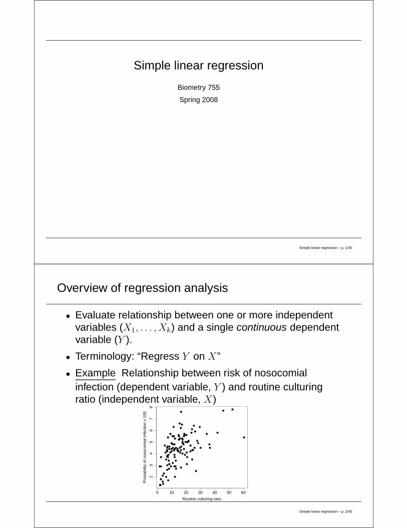
Visualizing SLR assumptions (cont.)
Normality
Normal data Non−normal data
“That looks normal?!!?”
Simple linear regression – p. 19/40
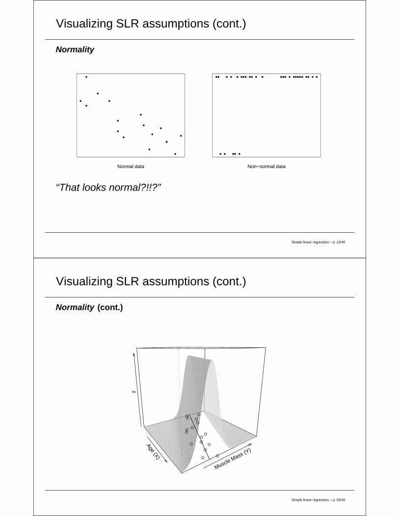
Visualizing SLR assumptions (cont.)
Normality (cont.)
Age (X)
Muscle Mass (Y)
z
Simple linear regression – p. 20/40

Model errors (εis) and residuals (ris)
Recall the form of the SLR model
yi = β0 + β1xi + εi.
By some simple algebra, we have
εi = yi − (β0 + β1xi)
= yi − E(yi|xi).
This gives us a simple way to estimate the errors in themodel. Namely,
εi = yi − yi
where yi = β0 + β1xi. The εis are called residuals. We write
ri = εi.
Simple linear regression – p. 21/40
More comments about errors and residuals
• yiind∼ Normal(β0 + β1xi, σ
2) is equivalent to
εiind∼ Normal(0, σ2).
• Why? (Intuitive answer) Recall that E(yi|xi), the averagevalue of yi given xi, is β0 + β1xi. Since yi = β0 + β1xi + εi,the average value of the errors must be zero. Otherwiseyi would, on average, be too large (average value of εi
positive) or too small (average value of εi negative).
• The residuals sum to zero.
Simple linear regression – p. 22/40

Residuals in SAS
proc reg data = one;model infrisk = cult/p;
run;
Simple linear regression – p. 23/40
Estimating spread around the regression line
Variance is estimated in the usual manner - that is, sum thesquared differences between the observed data points andtheir fitted values (based on the estimated regressionequation), and divide by an appropriate normalizing constant.
σ2 = s2 =
∑ni=1(yi − yi)
2
n − 2
• s2 is called the mean squared error or MSE.
• Since yi − yi = ri (the estimated error terms),∑ni=1(yi − yi)
2 is called the sum of squared errors or SSE.
• s2 = MSE = SSEn−2
Simple linear regression – p. 24/40

Some comments about σ2 = MSE
Q Why do we square the estimated errors?
A See the last comment on slide 22.
Q Why do we divide by n − 2? Doesn’t the usual formula forestimated variance divide by n − 1?
A We lose 2 degrees of freedom in estimating the meanresponse in a SLR. The usual formula you learn inintroductory statistics reflects the loss of a single degreeof freedom in estimating the mean.
Look at SAS output for SLR to see estimated SSE,denominator df, and MSE.
Simple linear regression – p. 25/40
Inference about the slope
The framework for the test of significance for the true slope isH0 : β1 = 0 versus HA : β1 �= 0. The test statistic is
t =β1 − 0
SE(β1
)
• SE(β1
)=
√MSEs2x(n−1)
is the standard error of β1
• s2x =
n
i=1(xi−x)2
n−1is the sample variance of the xis
• t ∼ tn−2 under H0
• A (1 − α) × 100 % confidence interval for β1 is
β1 ± tn−2,1−α/2 SE(β1
)
Simple linear regression – p. 26/40

Inference about the slope (cont.)
P-value and decision rule: Reject the null hypothesis if thep-value is less than α.
Conclusion: If the null is not rejected, this means that we havenot found a statistically significant linear relationship betweenX and Y (at level α). Note that there may be a relationship ofsome other kind (e.g. a non-linear relationship) between X
and Y , so failing to reject the null does not imply that there isno relationship.
If the null is rejected, this means that there is a significantlinear relationship between X and Y . Note, however, that thisdoes not imply that the linear model is the best or mostcorrect way to relate Y to X. The true relationship may besomething other than linear or it may include othercomponents in addition to a linear component.
Simple linear regression – p. 27/40
Inference about the intercept
Significance tests on the intercept are rarely performed. Thereason is that it is often difficult or impossible (or simply notrelevant) to collect sample data at or around x = 0. If thesample data does not include values near x = 0 (as is mostoften the case) you cannot trust a hypothesis test thatfocuses on that region. You do not have adequate data tomake good inference.
Simple linear regression – p. 28/40

SLR parameter estimates in SAS
proc reg data = one;model infrisk = cult/clb;
run;
Simple linear regression – p. 29/40
Inference about the regression line
In Slide 15, we saw that different random samples of datapoints from the same underlying model resulted in differentestimated regression lines. This implies that there is someinherent sampling variability associated with the regressionline itself. Just as a confidence interval provides informationabout the precision of point estimate, we would like atwo-dimensional equivalent to a CI that provides informationabout the precision of the fitted regression line. We call suchan interval a confidence band for the regression line, and itprovides an estimate of the uncertainty associated with aSLR.
Simple linear regression – p. 30/40

Inference about the regression line (cont.)
At each value of x = x0 (where x0 is the x-value associatedwith an observed data point), we compute the (1− α)× 100 %confidence interval
y|x0 ± tn−2,1−α/2 SE(y|x0)
• y|x0 is the fitted value at x0
• SE(y|x0) = s
√1n
+ (x0−x)2
(n−1)s2x
• s = σ =√
MSE
• s2x =
n
i=1(xi−x)2
n−1is the sample variance of the xis
At α = 0.05, we say that we are 95% confident that the trueregression line lies within the confidence band.
Simple linear regression – p. 31/40
Graphing the confidence band
Simple linear regression – p. 32/40

Graphing the confidence band - SAS code
ods html;ods graphics on;ods select Fit;
proc reg data = one;model infrisk = cult/clm;
run;
ods graphics off;ods html close;
Simple linear regression – p. 33/40
Prediction of a new value of y at x = x0
Often the goal of fitting a simple linear regression is to obtaina model that facilitates prediction. In SENIC example, wemight be interested in predicting the probability of nosocomialinfection at a local hospital where the routine culturing ratio is30. The obvious estimate is
Infrisk = 3.2 + 0.07 × 30 = 5.3.
Simple linear regression – p. 34/40

Prediction of a new value of y at x = x0 (cont.)
As always, we need a sense of the precision associated withthis predicted value. There are two sources of variabilityassociated with predicting the response:
1. The variability associated with the fitted regression line,illustrated in Slide 32. We estimate the square root of thisvariability with SE(y|x0), defined on Slide 31.
2. The variability associated with data points around the trueline, illustrated in Slide 20. We estimate this variabilitywith σ2 = MSE = s2, defined on Slide 24.
Simple linear regression – p. 35/40
Prediction of a new value of y at x0 (cont.)
The variability associated with predicting a response, y, atx = x0, is the sum of the variability due to fitting theregression line and the variability of the y values at x = x0
around the true regression line. We estimate this totalvariability as follows:
s2
(1
n+
(x0 − x)2
(n − 1)s2x
)︸ ︷︷ ︸
Var(y|x0)
+ s2︸︷︷︸σ2
= s2
(1 +
1
n+
(x0 − x)2
(n − 1)s2x
).
Simple linear regression – p. 36/40

Prediction of a new value of y at x0 (cont.)
Then a (1 − α) × 100% prediction interval is constructed usingthe formula
y|x0 ± tn−2,1−α/2 s
√1 +
1
n+
(x0 − x)2
(n − 1)s2x
.
We say that we are 95% confident that new responses will fallbetween the upper and lower limits of the interval.
Simple linear regression – p. 37/40
Graphing the prediction interval
Simple linear regression – p. 38/40

Graphing the confidence band - SAS code
ods html;ods graphics on;ods select Fit;
proc reg data = one;model infrisk = cult/cli;
run;
ods graphics off;ods html close;
Simple linear regression – p. 39/40
Interpretation
Confidence interval for mean at x = x0
Prediction interval at x = x0
Simple linear regression – p. 40/40