signals, spectra, signal processing ece 401 (tip reviewer)
DESCRIPTION
Signals, Spectra, Signal Processing ECE 401 (TIP Reviewer) James LindoTRANSCRIPT
1.1 Signals, Systems, and Signal Processing
*Signals - any physical quantity that varies with time, space or any other independent variable or variablesExamples:
Examples of Signals Independent Variable
Speech Signal, Electrocardiogram (ECG), Electroencephalogram (EEG)
Time
Image Signal Spatial Coordinates
*Speech signal, ECG and EEG are normally expressed as a sum of sinusoids of different amplitudes, frequencies and phases.
*may also be defined as a physical device or software that performs an operation on a signal*System - responds to a stimulus or force associated with signal generation
*Signal source - stimulus in combination with the system*Signal processing - linear or nonlinear operation on the signal*Algorithm - method or set of rules for implementing the system by a program that performs the corresponding mathematical operations.
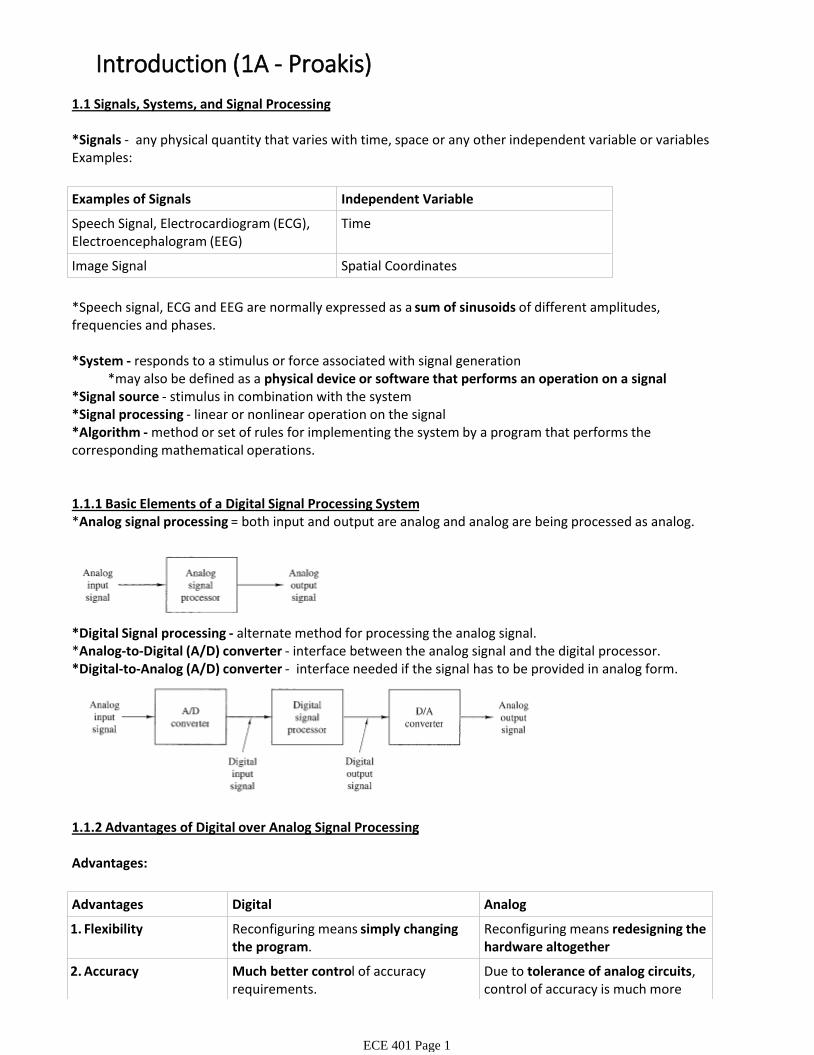
1.1.1 Basic Elements of a Digital Signal Processing System*Analog signal processing = both input and output are analog and analog are being processed as analog.
*Digital Signal processing - alternate method for processing the analog signal. *Analog-to-Digital (A/D) converter - interface between the analog signal and the digital processor. *Digital-to-Analog (A/D) converter - interface needed if the signal has to be provided in analog form.
1.1.2 Advantages of Digital over Analog Signal Processing
Advantages:
Advantages Digital Analog
Flexibility1. Reconfiguring means simply changing the program.
Reconfiguring means redesigning the hardware altogether
Accuracy2. Much better control of accuracy requirements.
Due to tolerance of analog circuits, control of accuracy is much more difficult.
Introduction (1A - Proakis)
ECE 401 Page 1
difficult.
Storage3. Can be easily stored on a magnetic media (tape or disk) without loss of signal fidelity.
Not possible.
Signal processing through Algorithm implementation
4. Can be done through a software on a digital computer.
Very difficult to do.
Cheaper5. Digital hardware is cheaper and flexibility for modifications.
More expensive hardware.
Limitations of Digital: (1) speed of operation of A/D converters and digital signal processors. (2) signals with extremely wide bandwidths
1.2 Classification of Signals
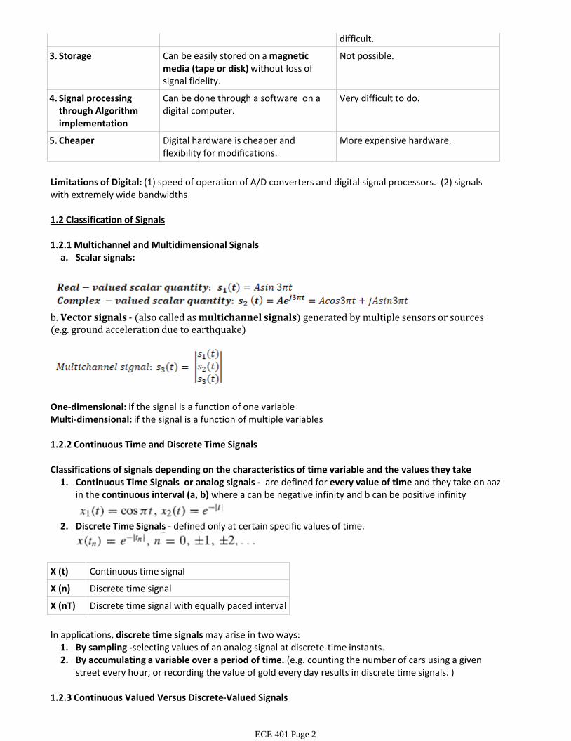
Scalar signals:a.1.2.1 Multichannel and Multidimensional Signals
b. Vector signals - (also called as multichannel signals) generated by multiple sensors or sources (e.g. ground acceleration due to earthquake)
One-dimensional: if the signal is a function of one variableMulti-dimensional: if the signal is a function of multiple variables
1.2.2 Continuous Time and Discrete Time Signals
Continuous Time Signals or analog signals - are defined for every value of time and they take on aaz in the continuous interval (a, b) where a can be negative infinity and b can be positive infinity
1.
Discrete Time Signals - defined only at certain specific values of time. 2.
Classifications of signals depending on the characteristics of time variable and the values they take
X (t) Continuous time signal
X (n) Discrete time signal
X (nT) Discrete time signal with equally paced interval
By sampling -selecting values of an analog signal at discrete-time instants. 1.By accumulating a variable over a period of time. (e.g. counting the number of cars using a given street every hour, or recording the value of gold every day results in discrete time signals. )
2.
In applications, discrete time signals may arise in two ways:
1.2.3 Continuous Valued Versus Discrete-Valued Signals
ECE 401 Page 2
Continuous Valued signal - if a signal takes on all possible values on a finite or an infinite range3.
Usually equidistance and can be expressed in integer multiplea.Discrete Valued signal - if a signal takes on values from a finite set of possible values4.
Digital signal - a discrete time signal having a set of discrete values Quantization - the approximation process of converting a continuous valued signal into a discrete-valuedsignal
1.2.4 Deterministic Versus Random SignalsSignal model - mathematical description of signalsDeterministic signals - any signal that can be uniquely described by an explicit mathematical expression , a table of data or a well-defined rule. In other words, all past, present and future values of the signal are known precisely and without uncertainty.
Random signals - cannot be described to a reasonable degree of accuracy by explicit mathematical formulas or such a description is too complicated. Unpredictable (e.g. output of a noise generator, seismic signal and speech signal)
ECE 401 Page 3
1.3 The Concept of Frequency in Continuous Time and Discrete-Time Signals
Frequency - closely related to a specific type of periodic motion called harmonic oscillation, which is described by sinusoidal functions.*inverse of time
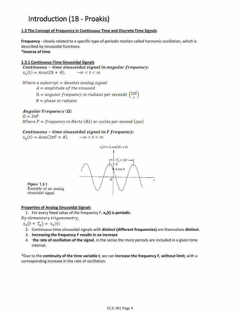
1.3.1 Continuous-Time Sinusoidal Signals
For every fixed value of the frequency F, xa(t) is periodic.1.Properties of Analog Sinusoidal Signals
Continuous-time sinusoidal signals with distinct (different frequencies) are themselves distinct.2.Increasing the frequency F results in an increase 3.the rate of oscillation of the signal, in the sense the more periods are included in a given time
interval.4.
*Due to the continuity of the time variable t, we can increase the frequency F, without limit, with a corresponding increase in the rate of oscillation.
Introduction (1B - Proakis)
ECE 401 Page 4
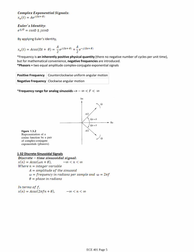
*Frequency is an inherently positive physical quantity (there no negative number of cycles per unit time), but for mathematical convenience, negative frequencies are introduced.*Phasors = two equal amplitude complex-conjugate exponential signals
Positive Frequency Counterclockwise uniform angular motion
Negative Frequency Clockwise angular motion
*Frequency range for analog sinusoids -->
1.32 Discrete-Sinusoidal Signals
ECE 401 Page 5
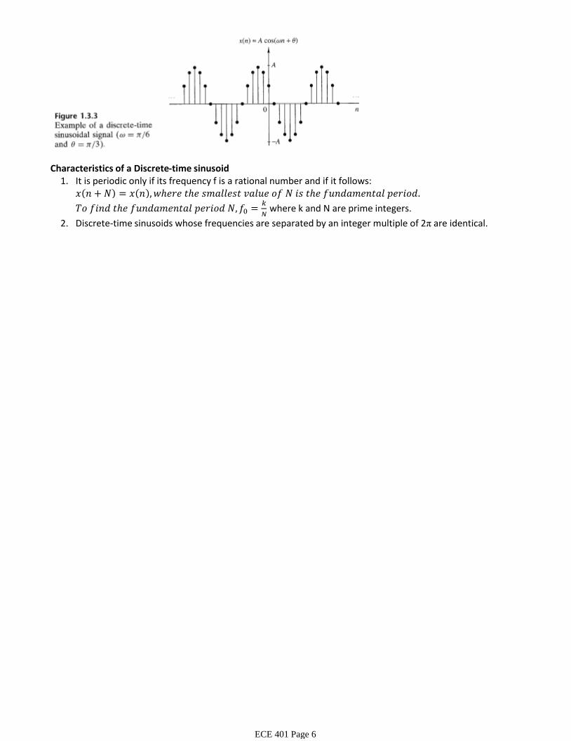
It is periodic only if its frequency f is a rational number and if it follows:1.
where k and N are prime integers.
Discrete-time sinusoids whose frequencies are separated by an integer multiple of 2π are identical.2.
Characteristics of a Discrete-time sinusoid
ECE 401 Page 6
2.1 Discrete-Time Signals
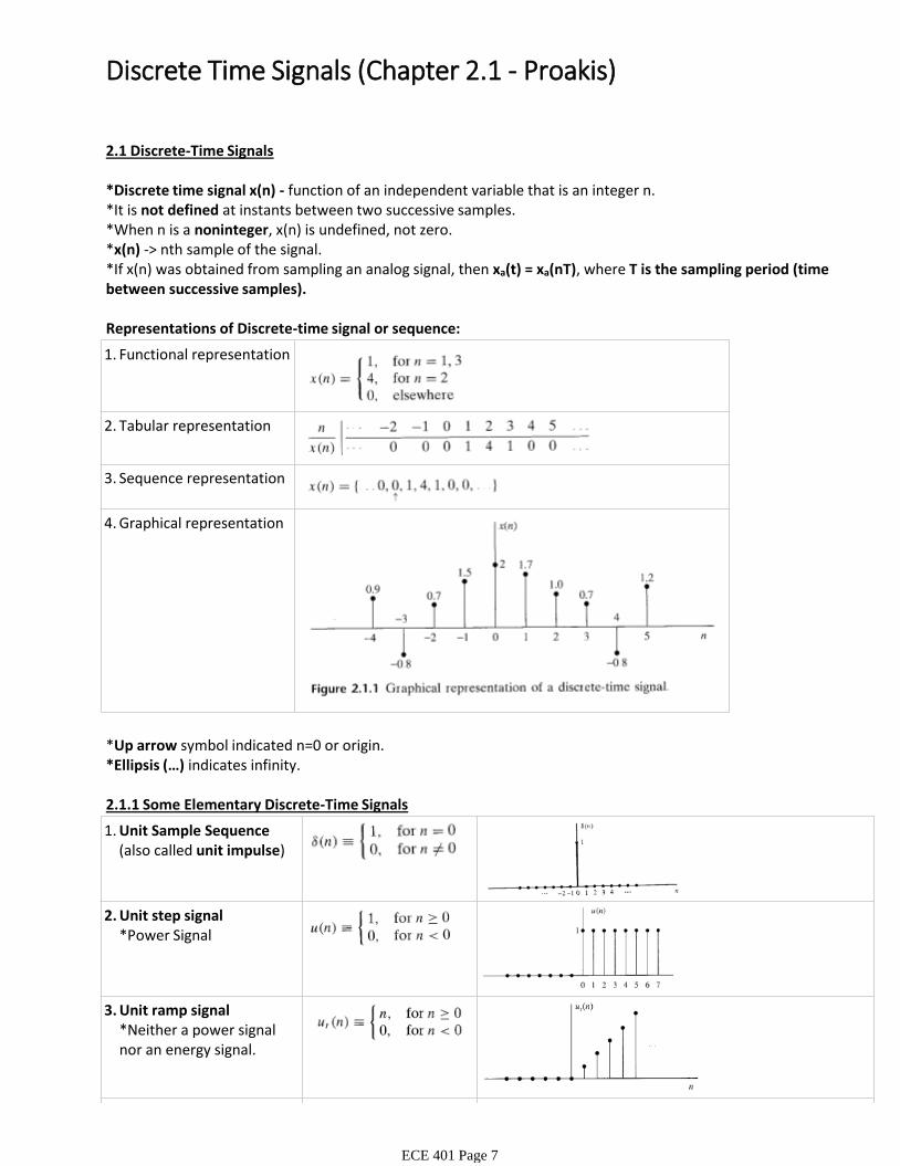
*Discrete time signal x(n) - function of an independent variable that is an integer n.*It is not defined at instants between two successive samples. *When n is a noninteger, x(n) is undefined, not zero.*x(n) -> nth sample of the signal.*If x(n) was obtained from sampling an analog signal, then xa(t) = xa(nT), where T is the sampling period (time between successive samples).
Representations of Discrete-time signal or sequence:
Functional representation1.
Tabular representation2.
Sequence representation3.
Graphical representation4.
*Up arrow symbol indicated n=0 or origin.*Ellipsis (…) indicates infinity.
2.1.1 Some Elementary Discrete-Time Signals
Unit Sample Sequence(also called unit impulse)
1.
Unit step signal2.*Power Signal
Unit ramp signal3.*Neither a power signal nor an energy signal.
Exponential signal4.
Discrete Time Signals (Chapter 2.1 - Proakis)
ECE 401 Page 7
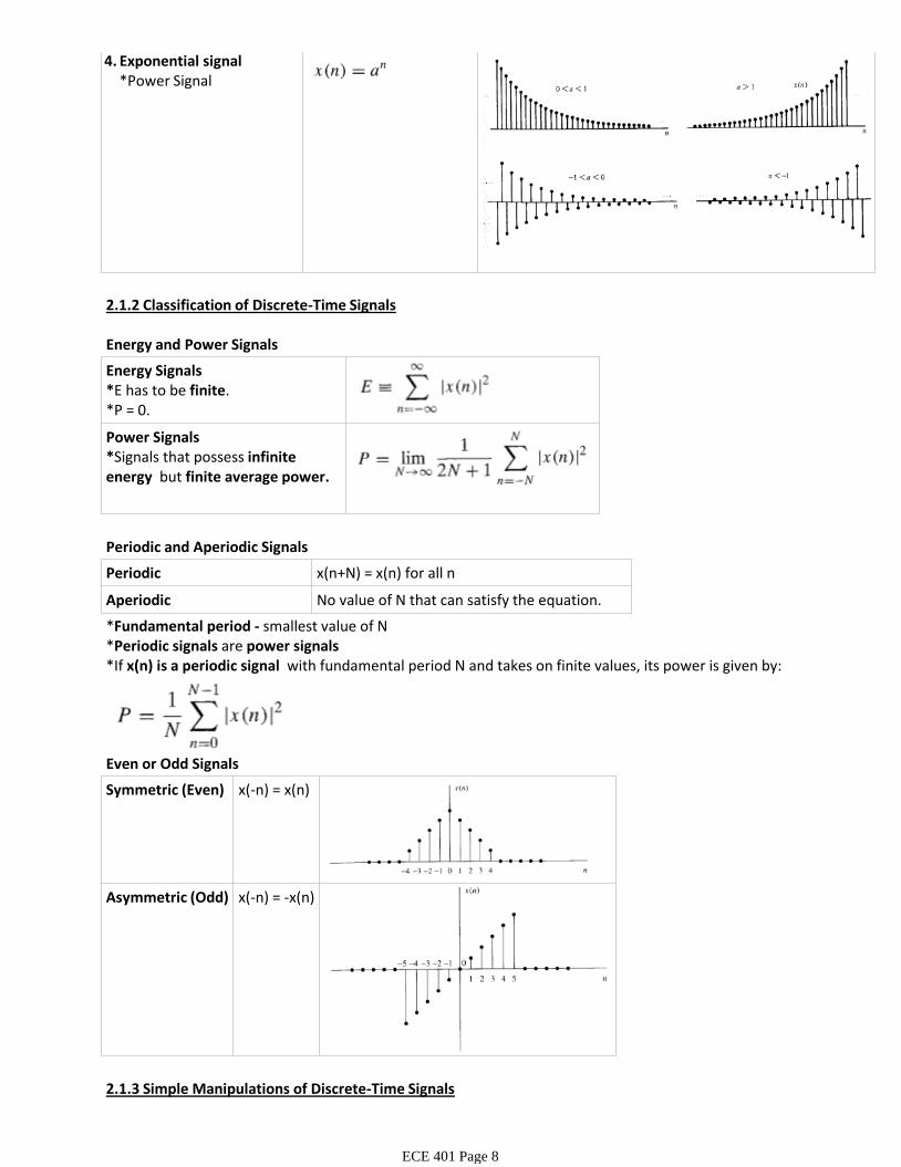
Exponential signal4.*Power Signal
2.1.2 Classification of Discrete-Time Signals
Energy and Power Signals
Energy Signals*E has to be finite.*P = 0.
Power Signals*Signals that possess infinite energy but finite average power.
Periodic and Aperiodic Signals
Periodic x(n+N) = x(n) for all n
Aperiodic No value of N that can satisfy the equation.
*Fundamental period - smallest value of N*Periodic signals are power signals*If x(n) is a periodic signal with fundamental period N and takes on finite values, its power is given by:
Even or Odd Signals
Symmetric (Even) x(-n) = x(n)
Asymmetric (Odd) x(-n) = -x(n)
2.1.3 Simple Manipulations of Discrete-Time Signals
ECE 401 Page 8
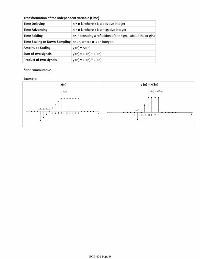
Transformation of the independent variable (time)
Time Delaying n = n-k, where k is a positive integer
Time Advancing n = n-k, where k is a negative integer
Time Folding n=-n (creating a reflection of the signal about the origin)
Time Scaling or Down-Sampling n=un, where u is an integer.
Amplitude Scaling y (n) = Ax(n)
Sum of two signals y (n) = x1 (n) + x2 (n)
Product of two signals y (n) = x1 (n) * x2 (n)
*Not commutative.
Example:
x(n) y (n) = x(2n)
ECE 401 Page 9

2.2 Discrete-Time Systems (Chapter 2.2 - Proakis)*Discrete Time System - a device or an algorithm that performs some prescribed operation on a discrete-time signal to produce another discrete time signalExcitation - incoming discrete time signal*Response - outcoming discrete time signal
*We say that the input x(n) is transformed by the system into a signal y(n), where T is the transformation or the operator
2.2.1 Input-Output Description of Systems
*Input-output description of a discrete-time system - consists of a mathematical expression or a rule, which explicitly defines the relations between the input and output systems. *Initial condition*Initially relaxed system - no prior excitation*Every system is relaxed at n is negative infinity, hence output is solely and uniquely determined by the given input.
2.2.2 Block Diagram Representation of Discrete-Time Systems*memoryless operation - no need to store neither of the sequences in order to perform the operation
Adder *memoryless operation
Constant Multiplier *memoryless operation
Signal Multiplier *memoryless operation
Unit Delay Element *requires memory*denoted by Z-1
Unit Advanced *requires memory*denoted by Z
static (memoryless) - if its output at any instant n depends at most on the input sample at the same time, but not on past or future samples of the input.
a.
dynamic (memory)b.
Static versus dynamic systems1.Classification of Systems
Discrete Time Systems
ECE 401 Page 10
Static
Static
Dynamic
Dynamic
Dynamic
Sample Problems:
a. Static
b. Dynamic
c. Static
d. Dynamic
e. Static
f. Static
g. Static
h. Static
i. Dynamic
j. Dynamic
k. Static
l. Dynamic
m. Static
n Static
Time-invariant versus time-variant systems2.Time-invariant - input-output characteristics do not change with time.a.*Dapat pareho ang values kapag dinelay lang versus kinalculate.Time variant - if there is a single value that disapproves it.b.
*Memory = Delay, Advanced, Folding, Internal Multiply and Summation
s
Time Invariant
Time Variant*n also changes!
Time Variant
Time Variant
Linear and NonLinear3.Linear system satisfies the superposition principlea.*Superposition principle: requires that the response of the system to a weighted sum of signals be equal to the corresponding weight sum of the responses (outputs) of the system to each of the individual input signals.
ECE 401 Page 11
sum of the responses (outputs) of the system to each of the individual input signals. *Transformation of two signals should be equal to the individually transformed signals!
*Multiplicative or scaling property and additivity propertyNon-linear - superposition test failed and zero input zero output failed!b.
Linear
Linear
Non-Linear
Linear
Non Linear (Failed the zero input-zero output test)
Causal versus Noncausal Systems:4.Causal - output of the system at any time n depends only on present and past inputsa.*x(n), x(n-1), x(n-2)NonCausal - depends on future inputsb.*x(n+1), x(n+2), x(n+3)*physically unrealizable!
x(n) - x(n-1) Causal
Causal
Causal
Noncausal*Advanced
Non Causal*If negative, it depends on its positive value.
Non Causal*If positive, it depends on the value of its double.
Non Causal*If negative, it depends on the value of its positive.
Sample Problems:
a. Causal
b. Non Causal
c. Causal
d. Non Causal
e. Causal
f. Causal
g. Causal
h. Causal
i. Non Causal
j. Non Causal
k. Causal
l. Non Causal
m. Causal
ECE 401 Page 12
n Causal
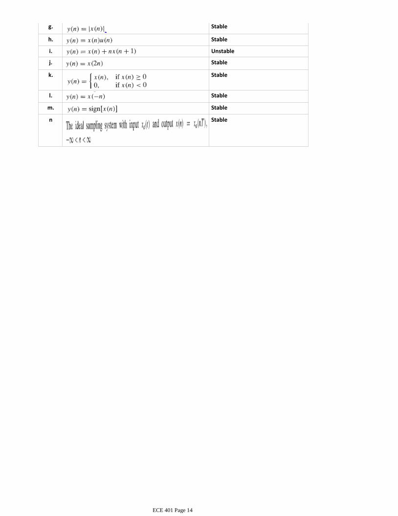
Stability versus Unstable Systems:5.
Stable - bounded input produced bounded output --> value approaches zero as time goes bya.Unstable - value approaches infinity or nonzero.b.
*Arbitrary relaxed system - bounded input-bounded output (BIBO) stable if and only if every bounded input produces a bounded output.
*Static, causal, stable
Sample Problems:
a. Stable*Less than 1, kapag n = infinity
b. Unstable*Summation
c. Stable*Less than 1, kapag n = infinity
d. Stable
e. Stable
f. Stable
g. Stable
h. Stable
i. Unstable
j. Stable
k. Stable
l. Stable
m. Stable
n Stable
a. Stable*Less than 1, kapag n = infinity
b. Unstable*Summation
c. Stable*Less than 1, kapag n = infinity
d. Stable
e. Stable
f. Stable
g. Stable
ECE 401 Page 13
g. Stable
h. Stable
i. Unstable
j. Stable
k. Stable
l. Stable
m. Stable
n Stable
ECE 401 Page 14
*Majority of the discrete time systems in practice are linear and shift invariant.*Discrete time signal can be expressed in the form of weighted impulses or weighted unit samples.*Linear Convolution: powerful analytical tool for studying LTI systems
*Linearity property states that the output due to a linear combination of inputs is the same as the sum of outputs due to individual inputs. (Distributive Property)*Scaling property states that if:
*Shift Invariance = if the excitation of the shift invariant system is delayed, then its response is also delayed by the same amount.
2.7.1 Discrete Time Signal as Weighted Impulses
*k = the range of the finite values.*x(k) = amplitude of the unit sample*δ (n-k) = location of the unit sample
2.7.2 Linear Convolution*Linear Convolution - is a very powerful technique used for the analysis of LTI systems.
*If x(n) is applied as an input:
*It can be expanded as:
*Since LTI systems are linear, the transformation T can be distributed:
*Since LTI systems are linear, the scaling property can also be applied, where the magnitudes can be treated as "coefficients".
*h(n) = unit sample response / impulse response of the system
Since LTI systems are shift invariant,
Substituting the response of the unit sample, we can derive the response of an LTI system, which is the linear
Linear Time Invariant (LTI) Systems (Chapter 2.7 - JS Chitode)
ECE 401 Page 15
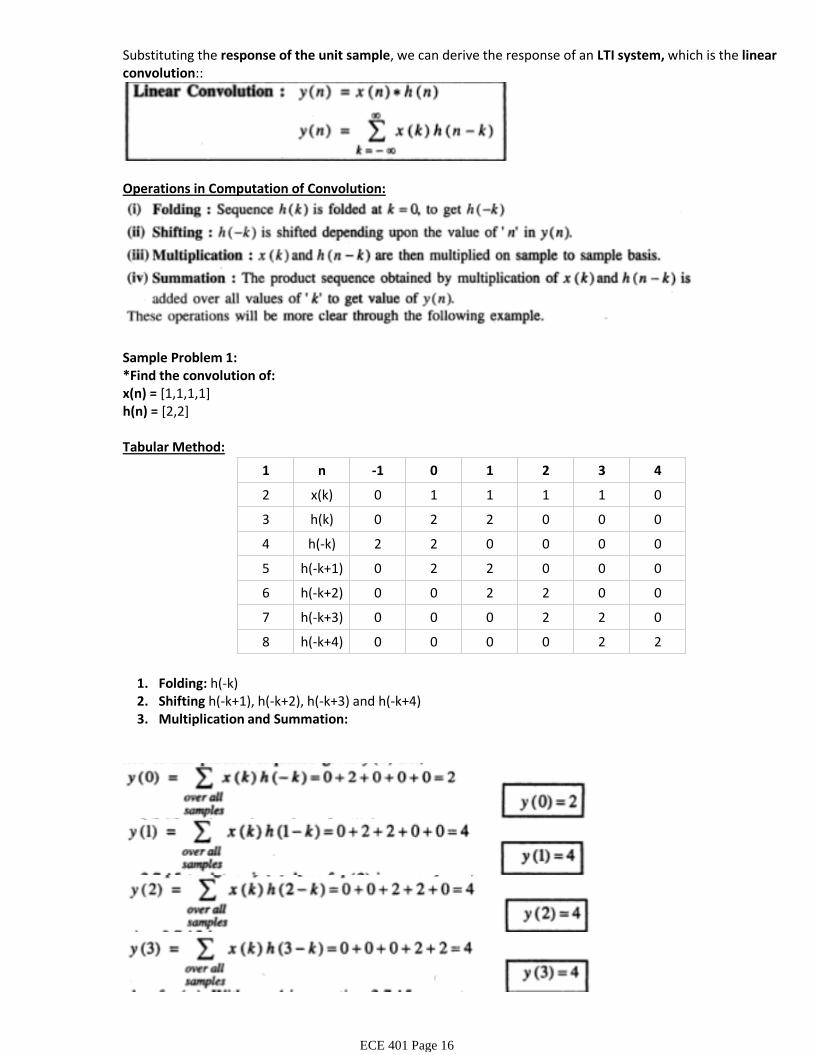
Substituting the response of the unit sample, we can derive the response of an LTI system, which is the linear convolution::
Operations in Computation of Convolution:
Sample Problem 1:*Find the convolution of:x(n) = [1,1,1,1]h(n) = [2,2]
Tabular Method:
1 n -1 0 1 2 3 4
2 x(k) 0 1 1 1 1 0
3 h(k) 0 2 2 0 0 0
4 h(-k) 2 2 0 0 0 0
5 h(-k+1) 0 2 2 0 0 0
6 h(-k+2) 0 0 2 2 0 0
7 h(-k+3) 0 0 0 2 2 0
8 h(-k+4) 0 0 0 0 2 2
Folding: h(-k)1.Shifting h(-k+1), h(-k+2), h(-k+3) and h(-k+4)2.Multiplication and Summation:3.
ECE 401 Page 16
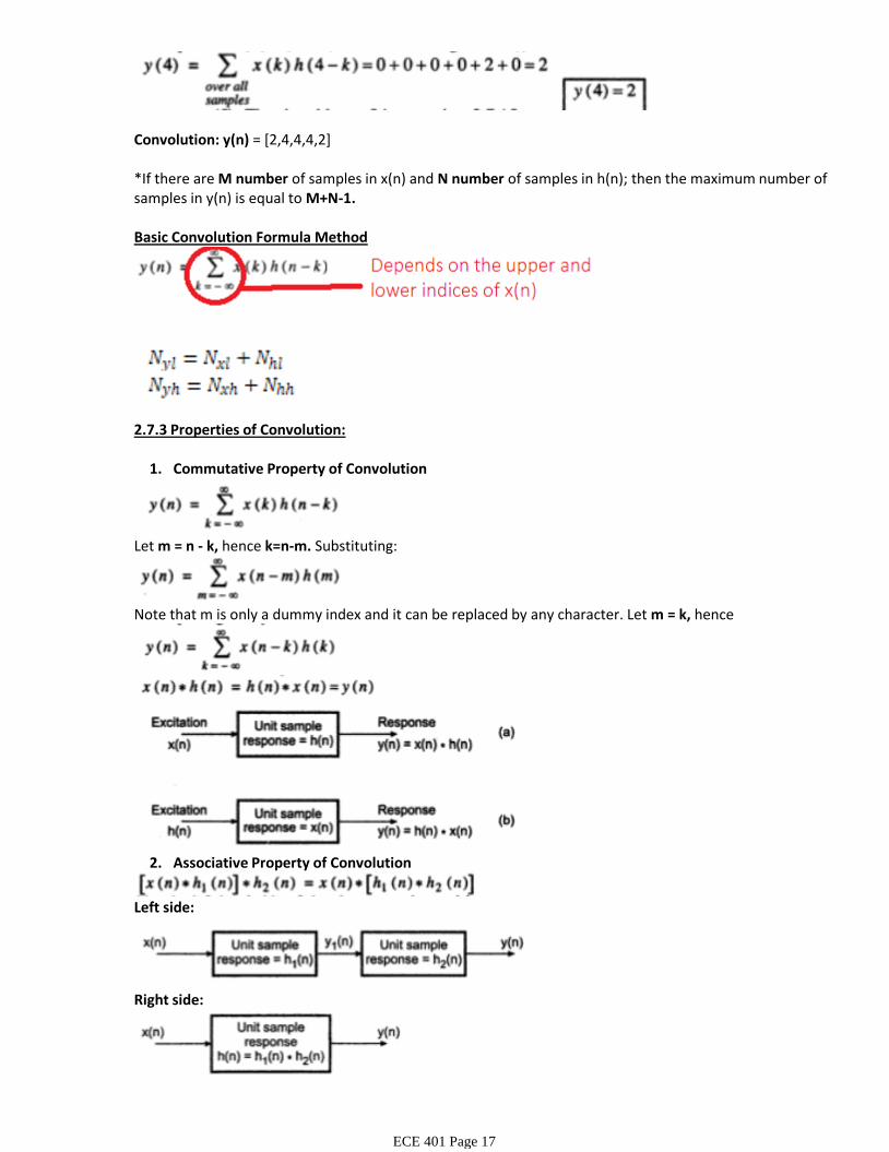
Convolution: y(n) = [2,4,4,4,2]
*If there are M number of samples in x(n) and N number of samples in h(n); then the maximum number of samples in y(n) is equal to M+N-1.
Basic Convolution Formula Method
2.7.3 Properties of Convolution:
Commutative Property of Convolution1.
Let m = n - k, hence k=n-m. Substituting:
Note that m is only a dummy index and it can be replaced by any character. Let m = k, hence
Associative Property of Convolution2.
Left side:
Right side:
*So if there are L numbers of LTI systems connected in cascade with unit sample responses of systems,
ECE 401 Page 17
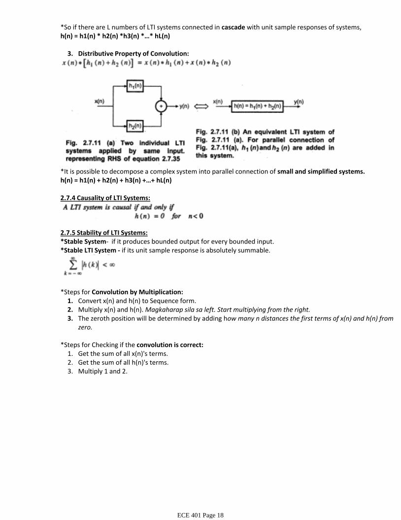
*So if there are L numbers of LTI systems connected in cascade with unit sample responses of systems,h(n) = h1(n) * h2(n) *h3(n) *…* hL(n)
Distributive Property of Convolution:3.
*It is possible to decompose a complex system into parallel connection of small and simplified systems.h(n) = h1(n) + h2(n) + h3(n) +…+ hL(n)
2.7.4 Causality of LTI Systems:
2.7.5 Stability of LTI Systems:*Stable System- if it produces bounded output for every bounded input. *Stable LTI System - if its unit sample response is absolutely summable.
Convert x(n) and h(n) to Sequence form.1.Multiply x(n) and h(n). Magkaharap sila sa left. Start multiplying from the right.2.The zeroth position will be determined by adding how many n distances the first terms of x(n) and h(n) from zero.
3.
*Steps for Convolution by Multiplication:
Get the sum of all x(n)'s terms.1.Get the sum of all h(n)'s terms.2.Multiply 1 and 2.3.
*Steps for Checking if the convolution is correct:
ECE 401 Page 18
ECE 401 Page 19
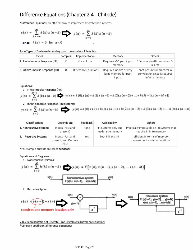
*Difference Equations: an efficient way to implement discrete time systems
Type Types of Systems depending upon the number of Samples:
Types Samples Implementation Memory Others:
Finite Impulse Response (FIR)1. M Convolution Requires M-1 past input memory
*Becomes inefficient when M is large
Infinite Impulse Response (IIR)2. ∞ Difference Equations Requires infinite or very large memory for past
inputs
*not possibly impractical in convolution since it requires
infinite memory
Finite Impulse Response (FIR)1.Equations:
Infinite Impulse Response (IIR) Systems:2.
Classifications Depends on: Feedback Applicability Others
Nonrecursive Systems1. Inputs (Past and present)
None FIR Systems only but needs large memory
Practically impossible on IIR systems that require infinite memory
Recursive Systems2. Inputs (Past and present) and Outputs
(Past)
Yes Both FIR and IIR efficient in terms of memory requirement and computations
*Past sample outputs are called feedback
Nonrecursive Systems:1.Equations and Diagrams:
Recursive System2.
2.8.5 Representation of Discrete Time Systems via Difference Equation:*Constant coefficient difference equations:
Difference Equations (Chapter 2.4 - Chitode)
ECE 401 Page 20
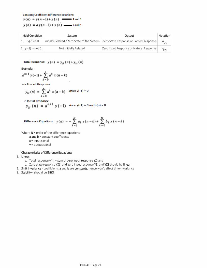
*Constant coefficient difference equations:
Initial Condition System Output Notation
y(-1) is 01. Initially Relaxed / Zero State of the System Zero State Response or Forced Response YZS
y(-1) is not 02. Not Initially Relaxed Zero Input Response or Natural Response YZI
Example:
a and b = constant coefficientsx = input signaly = output signal
Where N = order of the difference equations
Characteristics of Difference Equations:
Total response y(n) = sum of zero input response YZI anda.Zero state response YZS, and zero input response YZI and YZS should be linearb.
Linear: 1.
Shift Invariance - coefficients a and b are constants, hence won't affect time-invariance2.Stability - should be BIBO3.
ECE 401 Page 21
*FIR can be implemented through the convolution summation.*IIR is practically impossible to implement in convolution summation, since it requires an infinite number of memory locations, multiplications and additions.
2.4.1 Recursive and Nonrecursive Discrete-Time Systems*Convolution summation formula: expresses the output of an LTI system only in terms of the input signal
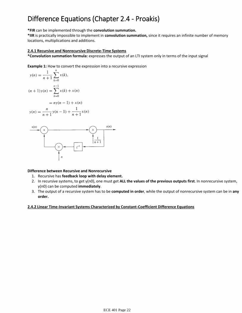
Example 1: How to convert the expression into a recursive expression
Recursive has feedback loop with delay element.1.In recursive systems, to get y(n0), one must get ALL the values of the previous outputs first. In nonrecursive system, y(n0) can be computed immediately.
2.
The output of a recursive system has to be computed in order, while the output of nonrecursive system can be in any order.
3.
Difference between Recursive and Nonrecursive
2.4.2 Linear Time-Invariant Systems Characterized by Constant-Coefficient Difference Equations
Difference Equations (Chapter 2.4 - Proakis)
ECE 401 Page 22
*In practice, system design and implementation are usually treated jointly rather than separately.
2.5.1 Structures for the Realization of Linear Time-Invariant Systems
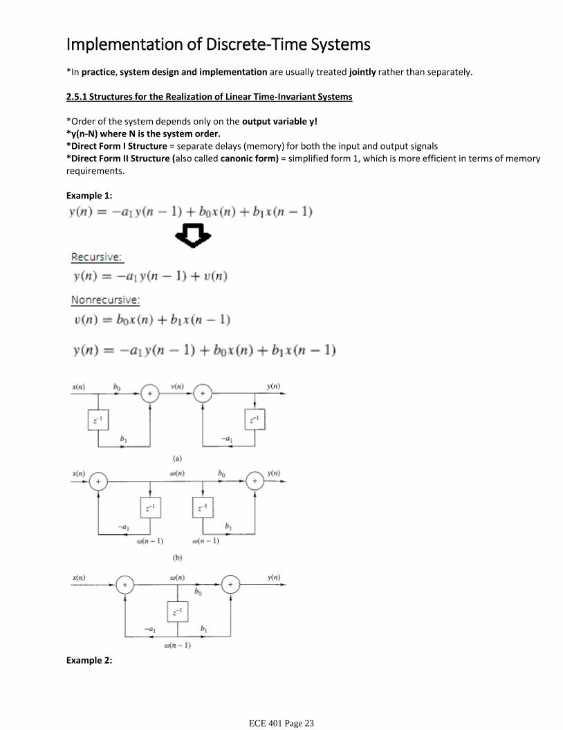
*Order of the system depends only on the output variable y! *y(n-N) where N is the system order.*Direct Form I Structure = separate delays (memory) for both the input and output signals*Direct Form II Structure (also called canonic form) = simplified form 1, which is more efficient in terms of memory requirements.
Example 1:
Example 2:
Implementation of Discrete-Time Systems
ECE 401 Page 23
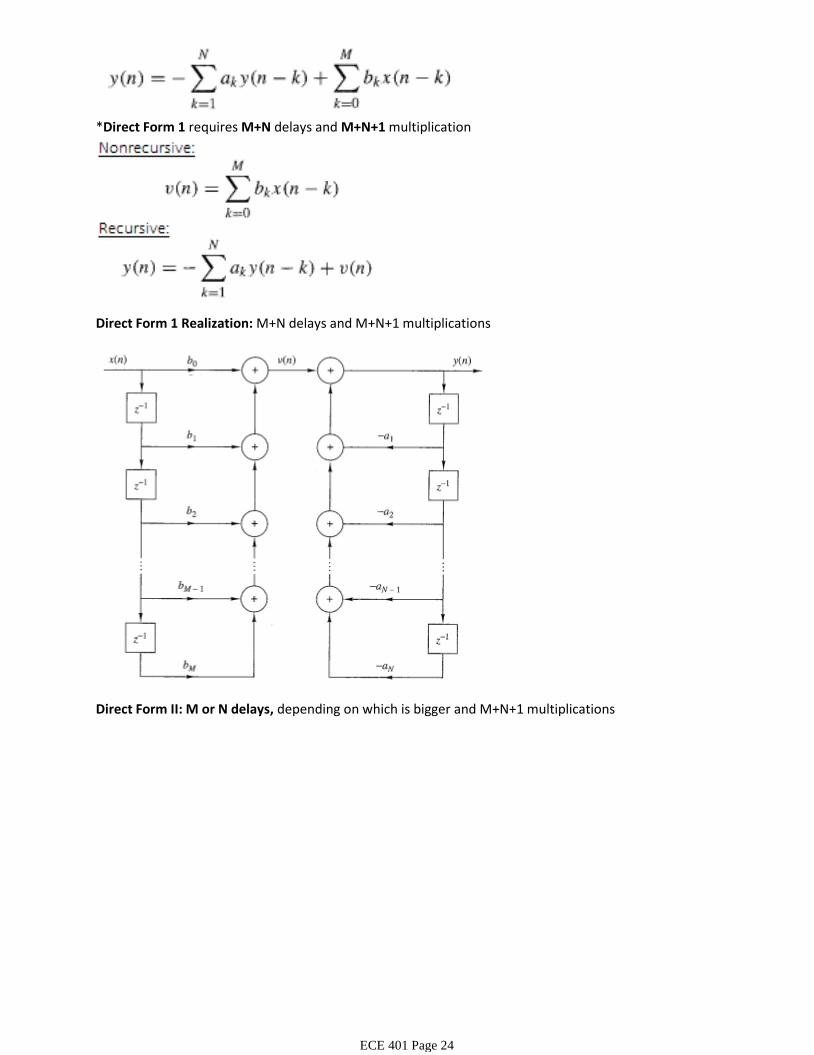
*Direct Form 1 requires M+N delays and M+N+1 multiplication
Direct Form 1 Realization: M+N delays and M+N+1 multiplications
Direct Form II: M or N delays, depending on which is bigger and M+N+1 multiplications
ECE 401 Page 24
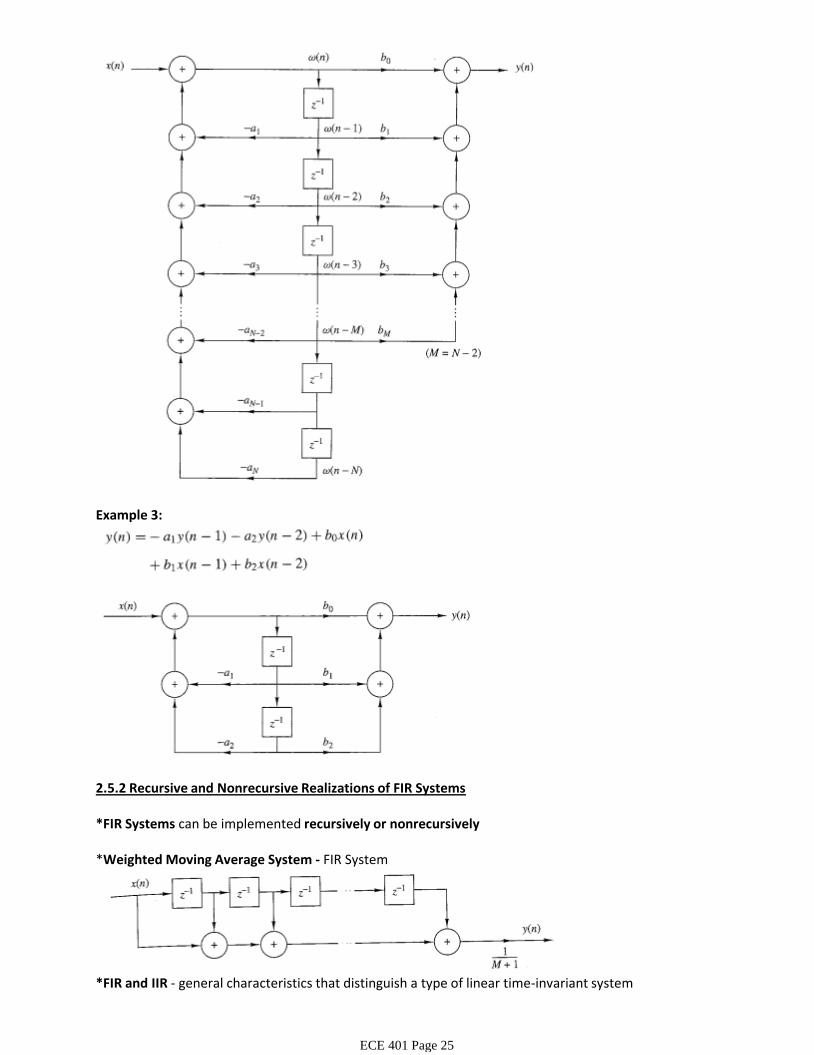
Example 3:
2.5.2 Recursive and Nonrecursive Realizations of FIR Systems
*FIR Systems can be implemented recursively or nonrecursively
*Weighted Moving Average System - FIR System
*FIR and IIR - general characteristics that distinguish a type of linear time-invariant system*Recursive and non-recursive - descriptions of the structures for realizing or implementing the system
ECE 401 Page 25

*Recursive and non-recursive - descriptions of the structures for realizing or implementing the system
ECE 401 Page 26
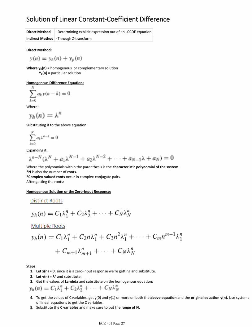
Direct Method Determining explicit expression out of an LCCDE equation-
Indirect Method Through Z-transform-
Direct Method:
Yp(n) = particular solutionWhere yh(n) = homogenous or complementary solution
Homogenous Difference Equation:
Where:
Substituting it to the above equation:
Expanding it:
Where the polynomials within the parenthesis is the characteristic polynomial of the system.*N is also the number of roots.*Complex-valued roots occur in complex-conjugate pairs.After getting the roots:
Homogenous Solution or the Zero-Input Response:
Let x(n) = 0, since it is a zero-input response we're getting and substitute.1.
Let y(n) = λn and substitute.2.Get the values of Lambda and substitute on the homogenous equation:3.
Steps
To get the values of C variables, get y(0) and y(1) or more on both the above equation and the original equation y(n). Use systems of linear equations to get the C variables.
4.
Substitute the C variables and make sure to put the range of N.5.Substitute any initial conditions.6.
Solution of Linear Constant-Coefficient Difference
ECE 401 Page 27
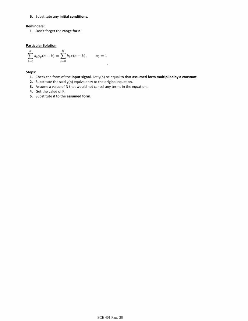
Substitute any initial conditions.6.
Don't forget the range for n!1.Reminders:
Particular Solution
Check the form of the input signal. Let y(n) be equal to that assumed form multiplied by a constant.1.Substitute the said y(n) equivalency to the original equation. 2.Assume a value of N that would not cancel any terms in the equation.3.Get the value of K.4.Substitute it to the assumed form.5.
Steps:
ECE 401 Page 28
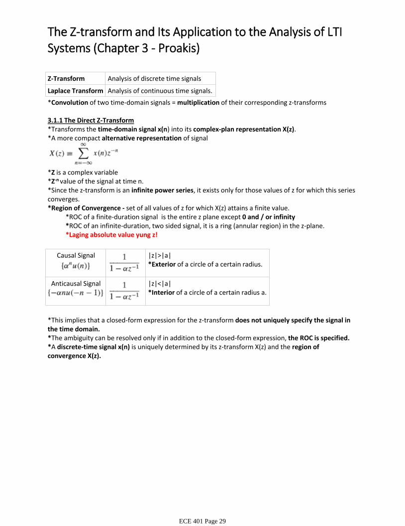
Z-Transform Analysis of discrete time signals
Laplace Transform Analysis of continuous time signals.
*Convolution of two time-domain signals = multiplication of their corresponding z-transforms
3.1.1 The Direct Z-Transform*Transforms the time-domain signal x(n) into its complex-plan representation X(z).*A more compact alternative representation of signal
*Z is a complex variable*Z-n value of the signal at time n.*Since the z-transform is an infinite power series, it exists only for those values of z for which this series converges.
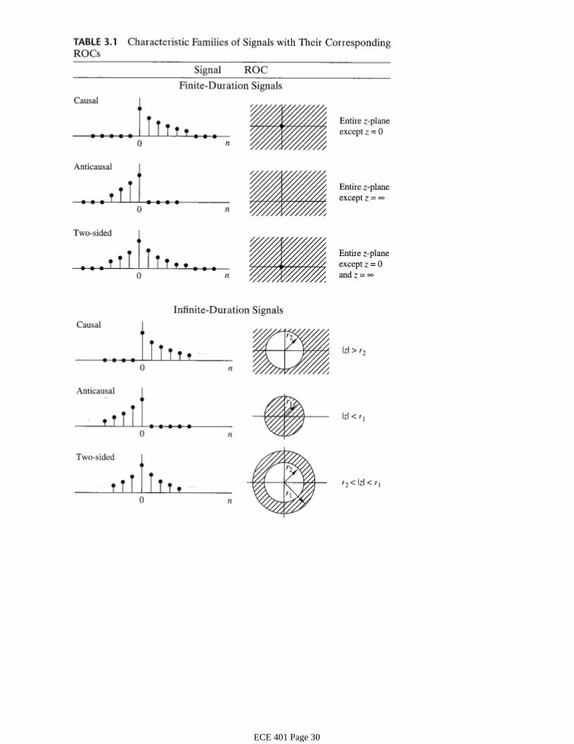
*ROC of a finite-duration signal is the entire z plane except 0 and / or infinity*ROC of an infinite-duration, two sided signal, it is a ring (annular region) in the z-plane. *Laging absolute value yung z!
*Region of Convergence - set of all values of z for which X(z) attains a finite value.
Causal Signal |z|>|a|*Exterior of a circle of a certain radius.
Anticausal Signal |z|<|a|*Interior of a circle of a certain radius a.
*This implies that a closed-form expression for the z-transform does not uniquely specify the signal in the time domain.*The ambiguity can be resolved only if in addition to the closed-form expression, the ROC is specified.*A discrete-time signal x(n) is uniquely determined by its z-transform X(z) and the region of convergence X(z).
The Z-transform and Its Application to the Analysis of LTI Systems (Chapter 3 - Proakis)
ECE 401 Page 29
ECE 401 Page 30
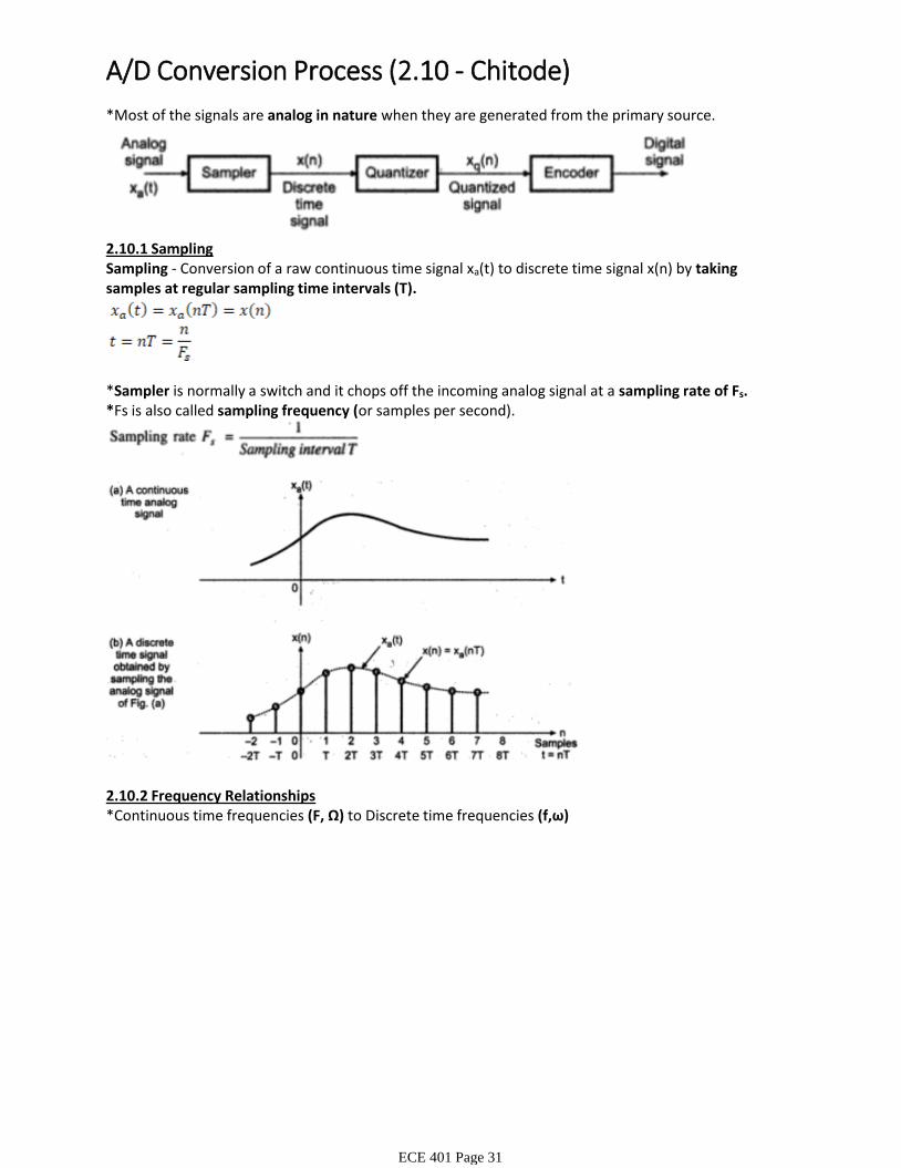
*Most of the signals are analog in nature when they are generated from the primary source.
2.10.1 SamplingSampling - Conversion of a raw continuous time signal xa(t) to discrete time signal x(n) by taking samples at regular sampling time intervals (T).
*Sampler is normally a switch and it chops off the incoming analog signal at a sampling rate of Fs.*Fs is also called sampling frequency (or samples per second).
2.10.2 Frequency Relationships*Continuous time frequencies (F, Ω) to Discrete time frequencies (f,ω)
A/D Conversion Process (2.10 - Chitode)
ECE 401 Page 31
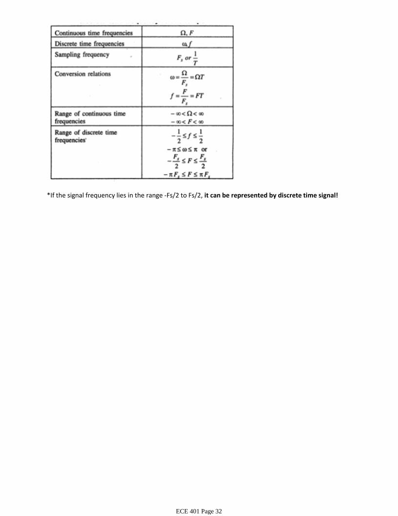
*If the signal frequency lies in the range -Fs/2 to Fs/2, it can be represented by discrete time signal!
ECE 401 Page 32

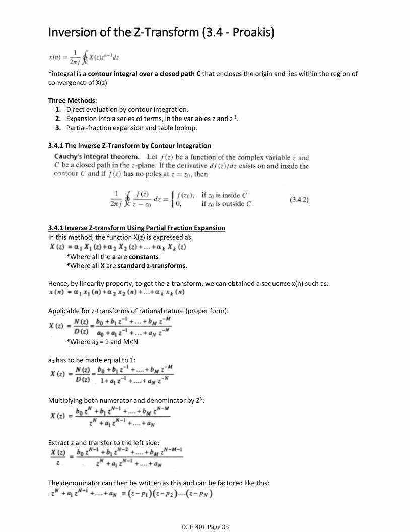
*integral is a contour integral over a closed path C that encloses the origin and lies within the region of convergence of X(z)
Direct evaluation by contour integration.1.Expansion into a series of terms, in the variables z and z-1.2.Partial-fraction expansion and table lookup.3.
Three Methods:
3.4.1 The Inverse Z-Transform by Contour Integration
3.4.1 Inverse Z-transform Using Partial Fraction ExpansionIn this method, the function X(z) is expressed as:
*Where all the a are constants*Where all X are standard z-transforms.
Hence, by linearity property, to get the z-transform, we can obtained a sequence x(n) such as:
Applicable for z-transforms of rational nature (proper form):
*Where a0 = 1 and M<N
a0 has to be made equal to 1:
Multiplying both numerator and denominator by ZN:
Extract z and transfer to the left side:
The denominator can then be written as this and can be factored like this:
Inversion of the Z-Transform (3.4 - Proakis)
ECE 401 Page 33

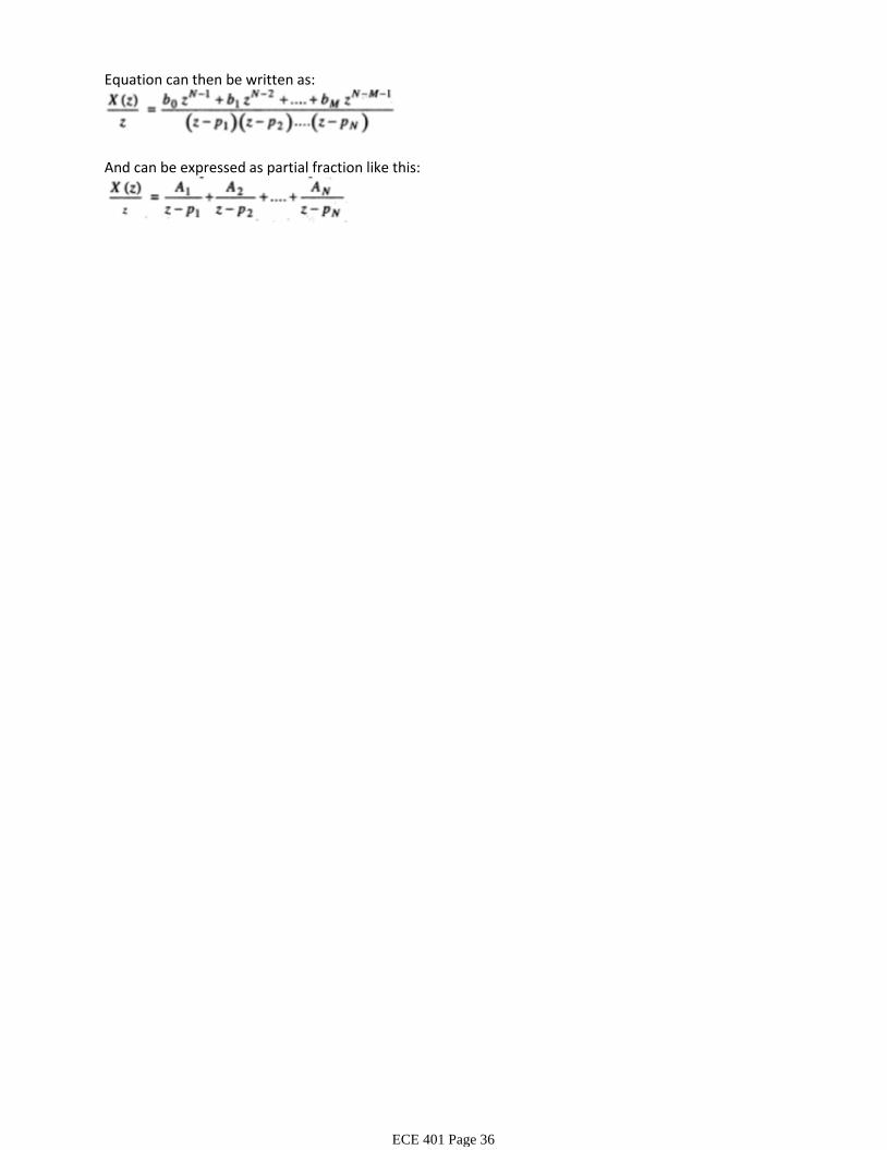
Equation can then be written as:
And can be expressed as partial fraction like this:
ECE 401 Page 34
*integral is a contour integral over a closed path C that encloses the origin and lies within the region of convergence of X(z)
Direct evaluation by contour integration.1.Expansion into a series of terms, in the variables z and z-1.2.Partial-fraction expansion and table lookup.3.
Three Methods:
3.4.1 The Inverse Z-Transform by Contour Integration
3.4.1 Inverse Z-transform Using Partial Fraction ExpansionIn this method, the function X(z) is expressed as:
*Where all the a are constants*Where all X are standard z-transforms.
Hence, by linearity property, to get the z-transform, we can obtained a sequence x(n) such as:
Applicable for z-transforms of rational nature (proper form):
*Where a0 = 1 and M<N
a0 has to be made equal to 1:
Multiplying both numerator and denominator by ZN:
Extract z and transfer to the left side:
The denominator can then be written as this and can be factored like this:
Inversion of the Z-Transform (3.4 - Proakis)
ECE 401 Page 35
Equation can then be written as:
And can be expressed as partial fraction like this:
ECE 401 Page 36
Sampling1.Quantization2.Coding3.
*Analog-to-digital signal conversion - converting a continuous time and amplitude signal into discrete-time and amplitude values.
Laboratory #4 (AD and DA Conversion)
ECE 401 Page 37
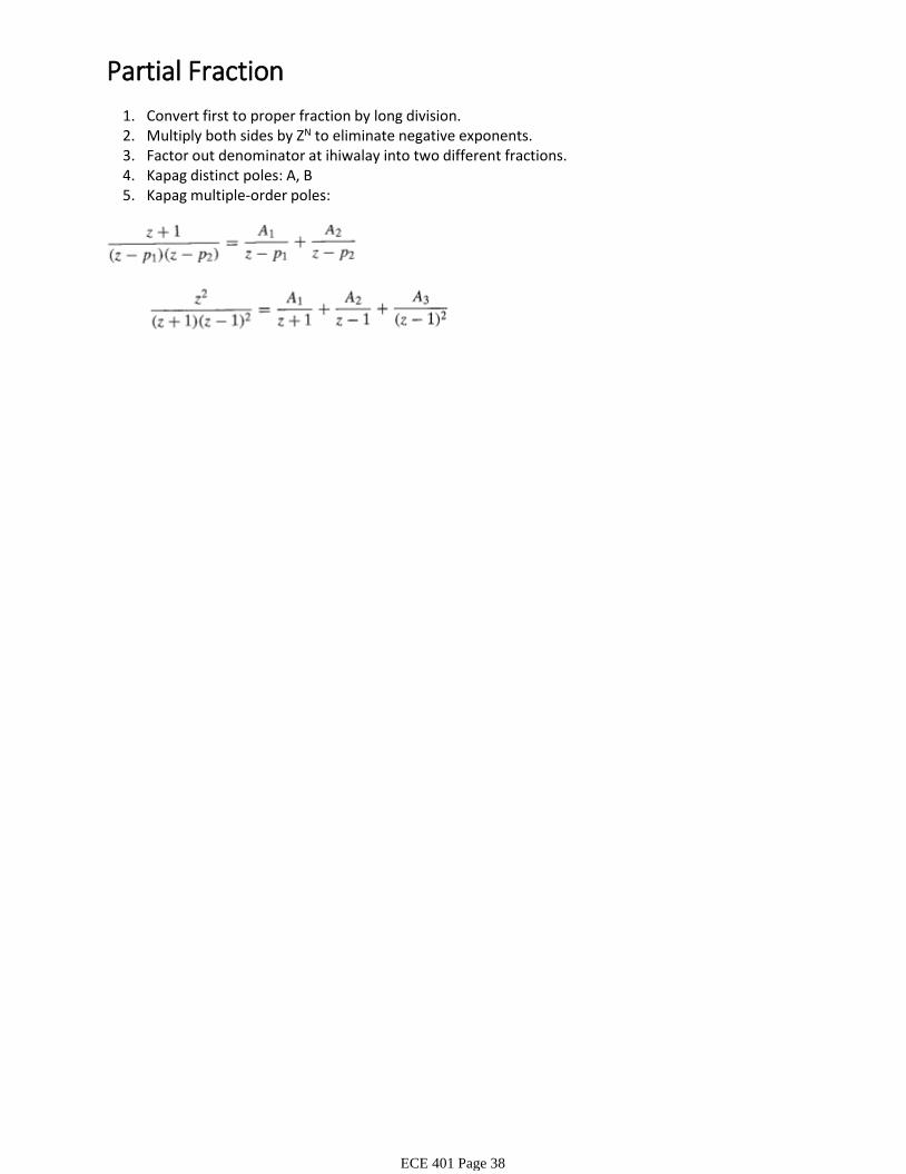
Convert first to proper fraction by long division.1.Multiply both sides by ZN to eliminate negative exponents. 2.Factor out denominator at ihiwalay into two different fractions. 3.Kapag distinct poles: A, B4.Kapag multiple-order poles: 5.
Partial Fraction
ECE 401 Page 38
Z-Transform TablesWednesday, October 07, 2015 10:50 AM
ECE 401 Page 39
ECE 401 Page 40