1

SIFT, SURF and Seasons: Long-term OutdoorLocalization Using Local Features

Christoffer Valgren Achim LilienthalApplied Autonomous Sensor Systems

Orebro UniversitySE-70182 Orebro, Sweden

christoffer.wahlgren@tech.oru.se, achim@lilienthals.de

Abstract— Local feature matching has become a commonlyused method to compare images. For mobile robots, a reliablemethod for comparing images can constitute a key componentfor localization and loop closing tasks. In this paper, we addressthe issues of outdoor appearance-based topological localizationfor a mobile robot over time. Our data sets, each consisting of alarge number of panoramic images, have been acquired overa period of nine months with large seasonal changes (snow-covered ground, bare trees, autumn leaves, dense foliage, etc.).Two different types of image feature algorithms, SIFT and themore recent SURF, have been used to compare the images. Weshow that two variants of SURF, called U-SURF and SURF-128,outperform the other algorithms in terms of accuracy and speed.

Index Terms— Outdoor Environments, Topological Localiza-tion, SIFT, SURF.

I. INTRODUCTION

Local feature matching has become an increasingly usedmethod for comparing images. Various methods have beenproposed. The Scale-Invariant Feature Transform (SIFT) byLowe [9] has, with its high accuracy and relatively low com-putation time, become the de facto standard. Some attemptsof further improvements to the algorithm have been made (forexample PCA-SIFT by Ke and Sukthankar [8]). Perhaps themost recent, promising approach is the Speeded Up RobustFeatures (SURF) by Bay et al. [3], which has been shownto yield comparable or better results to SIFT while having afraction of the computational cost [3, 2].

For mobile robots, reliable image matching can form thebasis for localization and loop closing detection. Local featurealgorithms have been shown to be a good choice for imagematching tasks on a mobile platform, as occlusions andmissing objects can be handled. In particular, SIFT appliedto panoramic images has been shown to give good resultsin indoor environments [1, 5] and also to some extent inoutdoor environments [12]. However, outdoor environmentsare very different from indoor environments. There are anumber of things that can alter the appearance of an outdoorscene: lighting conditions, shadows, seasonal changes, etc.All of these aspects makes image matching very difficult.1

Some attempts have been made to match outdoor imagesfrom different seasons. Zhang and Kosecka [14] focus on

1In some cases even impossible, since a snow-covered field might not haveany features.

recognizing buildings in images, using a hierarchical matchingscheme where a “localized color histogram” is used to limitthe search in an image database, with a final localizationstep based on SIFT feature matching. He et al. [7] also useSIFT features, but employ learning over time to find “featureprototypes” that can be used for localization.

In this paper, only local features extracted from panoramicimages will be used to perform topological localization. Sev-eral other works rely on similar techniques to do topologicalmapping and localization, for example Booij et al. [5], Sagueset al. [11] and Valgren et al. [12, 13]. The most recent workrelated to this paper is a comparative study for the localizationtask in indoor environments, published by Murillo et al. [10],where it is found that SURF outperforms SIFT because of itshigh accuracy and lower computation time.

The rest of the paper is structured as follows. In SectionII, the SIFT and SURF algorithms are discussed briefly. InSection III, the data sets used in the paper are described. InSection IV, the experiments are outlined and in Section V theresults of the experiments are presented.

II. FEATURE DETECTORS AND DESCRIPTORS

Both SIFT and SURF contain detectors that find interestpoints in an image. The interest point detectors for SIFT andSURF work differently. However, the output is in both cases arepresentation of the neighbourhood around an interest pointas a descriptor vector. The descriptors can then be compared,or matched, to descriptors extracted from other images.

SIFT uses a descriptor of length 128. Depending on theapplication, there are different matching strategies. A commonmethod, proposed by Lowe [9], is to compute the nearestneighbour of a feature, and then check if the second closestneighbour is further away than some threshold value. Otherstrategies consider only the nearest neighbour if the distanceis smaller than a threshold, as in Zhang and Kosecka [15], orcompute only the approximate nearest neighbour by using akd-tree, as in Beis and Lowe [4].

SURF has several descriptor types of varying length. In thispaper, we use regular SURF (descriptor length 64), SURF-128 (where the descriptor length has been doubled), and U-SURF (where the rotation invariance of the interest pointshave been left out, descriptor length is 64). U-SURF is usefulfor matching images where the viewpoints are differing by

2

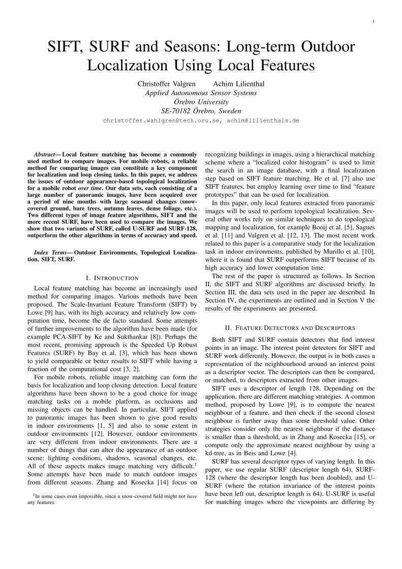
Data set Number of images Main characteristicsA 131 No foliage. Winter, snow-covered ground.

Overcast.B 80 Bright green foliage.

Bright sun and distinct shadows.C 597 Deep green foliage. Varying cloud cover.

D1 250 Early fall, some yellow foliage.Partly bright sun.

D2 195 Less leaves on trees, some on the ground.Bright sun.

D3 291 Mostly yellow foliage, many leaves on theground. Overcast.

D4 264 Many trees without foliage. Bright settingsun with some high clouds.

TABLE IREFERENCE TABLE FOR THE DATA SETS. THE NUMBER OF IMAGES IN THE

DATA SETS ONLY INCLUDES THE OUTDOOR IMAGES USED IN THIS PAPER.

a translation and rotation in the plane (i.e. planar motion).It should be noted that U-SURF is more sensitive to imageacquisition issues, such as the omnidirectional camera axisnot being perpendicular to the ground plane.

SURF can use the same matching scheme as SIFT, buthas one additional improvement. It includes the sign of theLaplacian, i.e. it allows for a quick distinction between brightfeatures on a dark background and dark features on a brightbackground. This allows for quicker feature matching thanSIFT, even in the case of SURF-128.

III. THE DATA SETS

Seven data sets were acquired over a period of nine months.The data sets span a part of the campus at Orebro University,in both indoor and outdoor locations. For the purpose of thispaper, all indoor images have been removed. The remainingimages form data sets, ranging from 80 images up to 597images, see Table I.

A. Details about the data sets

Data set A was acquired on a cloudy day in February, withbare trees and snow covered ground, see Figure 2 and 3.

Data set B was acquired on a warm May day, around noon,with a clear blue sky, see Figure 2.

Data set C, which is also the largest of the data sets andfunctions as our reference data set (it covers all places visitedin the other data sets, see Figure 1), was acquired during twodays in July, with a bright sky and varying cloud cover, seeFigure 2 and Figure 3.

Data sets D1, D2, D3 and D4 were all acquired duringOctober, with the purpose of capturing how the environmentchanges during Autumn. They have varying lighting condi-tions, and a different amount of leaves on the ground, seeFigure 2 and Figure 3.

The images were acquired every few meters; the distancebetween images varies between the data sets. The data sets donot all cover the same areas. For example, data set D1 doesnot include Positions 1 and 2 in Figure 1.

Position [m]

Pos

ition

[m]

−50 0 50 100

−50

0

50

Dataset ADataset BDataset CDataset D1Dataset D2Dataset D3Dataset D4

Position 1

Position 2

Position 3

Position 4

Position 5

Fig. 1. Aerial image, illustrating the coverage of the data sets. The positionshave been acquired by adjusting odometry measurements to fit the map.Approximate total path length for data set C is 1.1 km. Circles indicate theapproximate positions 1 to 5 used in Experiment 2.

B. Data set acquisition

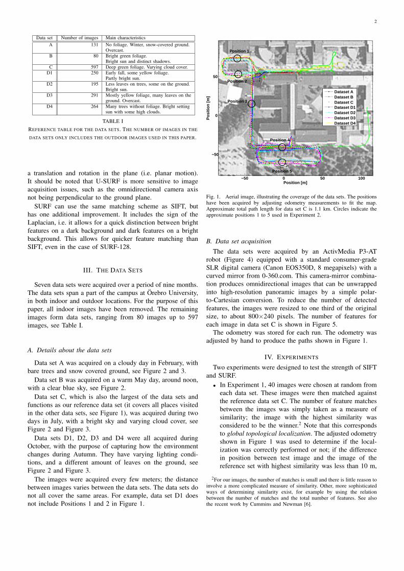
The data sets were acquired by an ActivMedia P3-ATrobot (Figure 4) equipped with a standard consumer-gradeSLR digital camera (Canon EOS350D, 8 megapixels) with acurved mirror from 0-360.com. This camera-mirror combina-tion produces omnidirectional images that can be unwrappedinto high-resolution panoramic images by a simple polar-to-Cartesian conversion. To reduce the number of detectedfeatures, the images were resized to one third of the originalsize, to about 800×240 pixels. The number of features foreach image in data set C is shown in Figure 5.

The odometry was stored for each run. The odometry wasadjusted by hand to produce the paths shown in Figure 1.

IV. EXPERIMENTS

Two experiments were designed to test the strength of SIFTand SURF.

• In Experiment 1, 40 images were chosen at random fromeach data set. These images were then matched againstthe reference data set C. The number of feature matchesbetween the images was simply taken as a measure ofsimilarity; the image with the highest similarity wasconsidered to be the winner.2 Note that this correspondsto global topological localization. The adjusted odometryshown in Figure 1 was used to determine if the local-ization was correctly performed or not; if the differencein position between test image and the image of thereference set with highest similarity was less than 10 m,

2For our images, the number of matches is small and there is little reason toinvolve a more complicated measure of similarity. Other, more sophisticatedways of determining similarity exist, for example by using the relationbetween the number of matches and the total number of features. See alsothe recent work by Cummins and Newman [6].

3

Fig. 2. Data sets A, B, C, D2, D3 and D4. Position 1.

the localization was considered successful. A localizationwas also deemed correct if a set of images shared thehighest score, and a correct image match was found inthe set.

• In Experiment 2, five viewpoints (Position 1 through 5 inFigure 1) that occurred in several of the data sets werecompared using SIFT and SURF. The number of correctcorrespondences and the total number of correspondenceswere recorded for each viewpoint. In this experiment, werely on a human judge to determine the correctness ofindividual feature matches.

The binaries published on the web sites for SIFT3 andSURF4 were used to compute the feature descriptors. BothSIFT and SURF utilize feature vectors, so the same code wasused to perform the image matching, with the exception that

3http://www.cs.ubc.ca/∼lowe/keypoints/4http://www.vision.ee.ethz.ch/∼surf/

Fig. 3. Data sets A, C, D1, D2, D3 and D4. Position 5.

we introduced a check for the sign of the Laplacian for theSURF features. A simple brute force, nearest-neighbour search(using the Euclidean distance) was performed. Lowe found avalue of 0.8 for the relation between the nearest and secondnearest neighbour [9] to be suitable. In the paper by Bay etal. [3], a value of 0.7 is used for the SURF descriptor.

Since it is not the purpose of this paper to tune a particularmatching scheme to our data sets, we have used both 0.7and 0.8 as threshold in the experiments. However, it is likelythat the threshold for the nearest-neighbour matching mightinfluence the result; this is something that we leave for futurework.

While an epipolar constraint (as in Booij et al. [5]) could beapplied to improve the matching rate, this might give an unfairadvantage to one of the algorithms. In particular SURF mightsuffer from this, since the SIFT keypoint detector returns manymore interest points in the images, see Figure 5.

4

Fig. 4. The mobile robot platform, used to acquire the images used in thispaper. The omnidirectional camera can be seen in the top left part of theimage.

0 100 200 300 400 500 6000

200

400

600

800

1000

1200

1400

1600

1800

2000

Image index [−]

Num

ber

of in

tere

st p

oint

s [−

]

SIFTSURF

Fig. 5. The number of interest points for reference data set C. Note that thedifferent versions of SURF use the same feature detector and therefore havethe same number of interest points.

V. RESULTS

A. Experiment 1

The charts in Figure 6 and 7 show the results from Ex-periment 1, using thresholds of 0.7 and 0.8, respectively. Astriking result is that feature matching alone cannot, in general,be used to perform correct single image localization whenthe data sets are acquired over a longer period of time. Thelocalization rate is too low – even the best algorithm doesnot reach higher than about 40% in one of the cases. On theother hand, this is perhaps not surprising, since the dynamicsof outdoor environments sometimes can leave even humanslost.

Another interesting result is that SIFT performs worst fortwo of the data sets, and never gives the highest localizationrate (exclusively).

SURF-128 outperforms the other algorithms, giving thehighest localization rate for all data sets except data set B.

It is notable that the low localization rates of data set B

Fig. 6. Result for Experiment 1. 40 random images from each data set werelocalized with respect to the reference data set C. The bar chart shows thelocalization rate, using a threshold of 0.7.

Fig. 7. Result for Experiment 1. 40 random images from each data set werelocalized with respect to the reference data set C. The bar chart shows thelocalization rate, using a threshold of 0.8.

and D2 coincide with a qualitative change in the appearanceof the environment; both data set B and D2 were acquired indirect sun light that casts long shadows and causes the whitebuildings to be very bright, see Figure 2.

B. Experiment 2

The chart matrices shown in Figures 8 through 12 show theresults from Experiment 2 using a threshold of 0.7 (results byusing a threshold of 0.8 are omitted for space reasons, but arequalitatively the same). Again, data sets B and D2 have a lownumber of matches. It is also, as one might expect, fairly hardto match the snow-covered data set A to the other data sets.

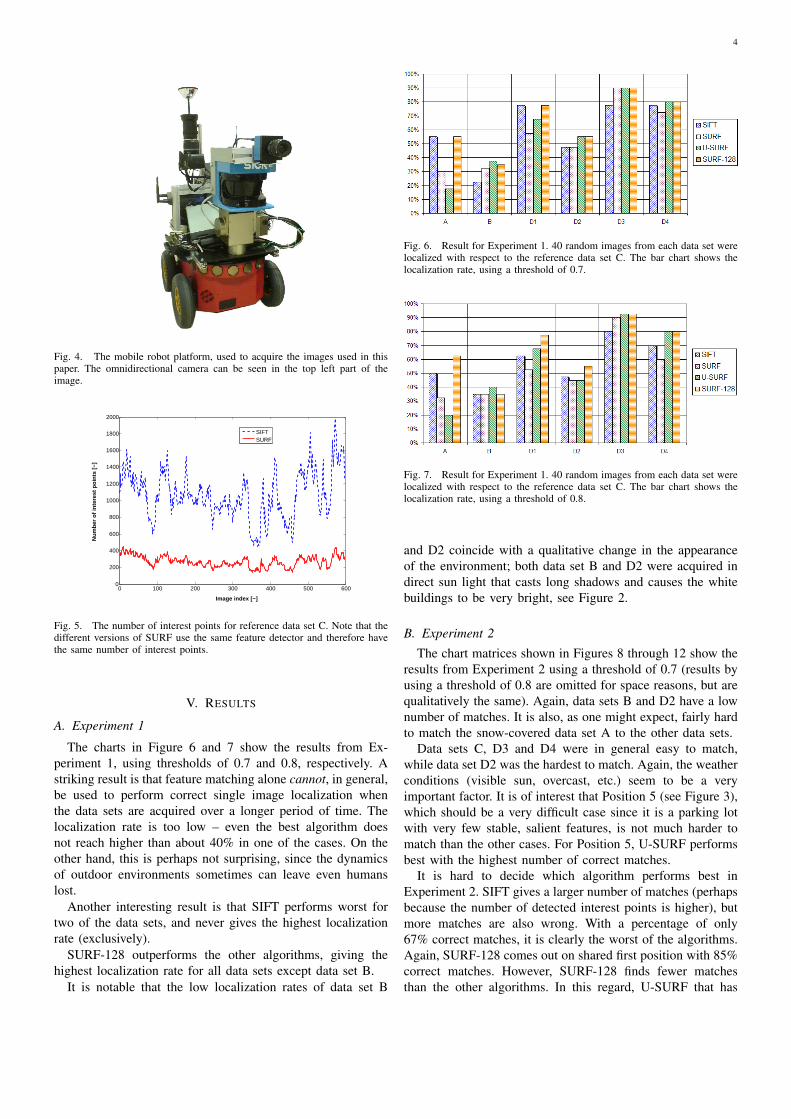
Data sets C, D3 and D4 were in general easy to match,while data set D2 was the hardest to match. Again, the weatherconditions (visible sun, overcast, etc.) seem to be a veryimportant factor. It is of interest that Position 5 (see Figure 3),which should be a very difficult case since it is a parking lotwith very few stable, salient features, is not much harder tomatch than the other cases. For Position 5, U-SURF performsbest with the highest number of correct matches.

It is hard to decide which algorithm performs best inExperiment 2. SIFT gives a larger number of matches (perhapsbecause the number of detected interest points is higher), butmore matches are also wrong. With a percentage of only67% correct matches, it is clearly the worst of the algorithms.Again, SURF-128 comes out on shared first position with 85%correct matches. However, SURF-128 finds fewer matchesthan the other algorithms. In this regard, U-SURF that has

5

Algorithm Total matches Total correct matches Percentage correctSIFT 1222 824 67%

SURF 598 473 79%U-SURF 760 648 85%

SURF-128 531 452 85%

TABLE IITOTAL NUMBER OF MATCHES FOR EXPERIMENT 2, WITH THRESHOLD 0.7.

0

5B

0

1020

C

05

10

D2

0

20

D3

0

10

D4

05

10

05

10

05

10

0

5

05

1015

0

50

0

50

0

10

05

10

0

20

SIFTSURFU−SURFSURF−128

A

B

C

D2

D3

Fig. 8. Result for Experiment 2, position 1. The same approximate viewpointwas selected from several data sets, and the matches were evaluated bya human judge. Each bar chart shows the matches between two data sets(indicated by labels on rows/columns). In the charts, darker color indicatescorrect matches, brighter color indicates total number of matches.

a high number of both found and correct matches will be thewinner. See Table II.

C. Time consumption

The computational cost for SIFT is much greater thanSURF.

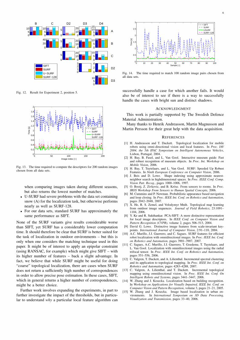
Figure 13 shows the computation time required for thedetection of features for the different algorithms. U-SURF isfastest, followed by SURF, SURF-128 and finally SIFT, whichis nearly three times as slow.

Figure 14 shows the computation time required to do featurematching for the different algorithms. The times required forthe SURF variants are all at around 0.25 seconds, while SIFTvaries from 0.5 to 2 seconds (with a mean of about 1.1seconds).

VI. CONCLUSIONS

In this paper, we have investigated how local featurealgorithms can cope with large outdoor environments thatchange over the year. The results from our experiments canbe summarized as follows:

• It is not, with the current algorithms, possible to do singlepanoramic image localization based only on appearancein large outdoor environments with seasonal changes.

• SURF-128 outperforms the other algorithms for thesedata sets, at least in terms of localization. SURF-128also has the highest percentage of correct feature matches

0

5

B

0

10

C

05

10

D2

05

10

D3

05

10

D4

0

5

0

5

0

510

0

5

0

510

0

10

20

05

10

0

5

05

10

01020

SIFTSURFU−SURFSURF−128

A

B

C

D2

D3

Fig. 9. Result for Experiment 2, position 2.

0

10

B

0

10

C

0

5

D2

01020

D3

0

5

D4

0

10

0

5

0

50

01020

0

10

0

20

0

20

40

05

1015

0

10

20

0

20

SIFTSURFU−SURFSURF−128

A

B

C

D2

D3

Fig. 10. Result for Experiment 2, position 3.

05

10

B

0

5

C

0

5

D2

05

10

D3

05

1015

D4

0

5

0

5

0

20

0

5

0

510

0

5

0

5

0

1

2

0

2

4

0

510

SIFTSURFU−SURFSURF−128

A

B

C

D2

D3

Fig. 11. Result for Experiment 2, position 4.

6

05

10

B

05

10

C

0

5

D2

01020

D3

05

1015

D4

0

2040

0

5

01020

05

10

0

5

01020

05

10

0123

0

2

4

05

10

SIFTSURFU−SURFSURF−128

A

B

C

D2

D3

Fig. 12. Result for Experiment 2, position 5.

0 50 100 150 2000

0.2

0.4

0.6

0.8

1

1.2

1.4

1.6

1.8

2

Image index [−]

Tim

e [s

]

SIFTSURFU−SURFSURF−128

Fig. 13. The time required to compute the descriptors for 200 random imageschosen from all data sets.

when comparing images taken during different seasons,but also returns the lowest number of matches.

• U-SURF had severe problems with the data set containingsnow (A) for the localization task, but otherwise performsnearly as well as SURF-128.

• For our data sets, standard SURF has approximately thesame performance as SIFT.

None of the SURF variants give results considerable worsethan SIFT, yet SURF has a considerably lower computationtime. It should therefore be clear that SURF is better suited forthe task of localization in outdoor environments – but this isonly when one considers the matching technique used in thispaper. It might be of interest to apply an epipolar constraint(using RANSAC, for example) which might give SIFT – withits higher number of features – back a slight advantage. Infact, we believe that while SURF might be useful for doing“coarse” topological localization, there are cases when SURFdoes not return a sufficiently high number of correspondencesin order to allow precise pose estimation. In these cases, SIFT,which in general returns a higher number of correspondences,might be a better choice.

Further work involves expanding the experiments, in part tofurther investigate the impact of the thresholds, but in particu-lar to understand why a particular local feature algorithm can

0 10 20 30 40 50 60 70 80 90 1000

0.5

1

1.5

2

2.5

3

Sample [−]

Tim

e [s

]

SIFTSURFUSURFSURF−128

Fig. 14. The time required to match 100 random image pairs chosen fromall data sets.

successfully handle a case for which another fails. It wouldalso be of interest to see if there is a way to successfullyhandle the cases with bright sun and distinct shadows.

ACKNOWLEDGMENT

This work is partially supported by The Swedish DefenceMaterial Administration.

Many thanks to Henrik Andreasson, Martin Magnusson andMartin Persson for their great help with the data acquisition.

REFERENCES

[1] H. Andreasson and T. Duckett. Topological localization for mobilerobots using omni-directional vision and local features. In Proc. IAV2004, the 5th IFAC Symposium on Intelligent Autonomous Vehicles,Lisbon, Portugal, 2004.

[2] H. Bay, B. Fasel, and L. Van Gool. Interactive museum guide: Fastand robust recognition of museum objects. In Proc. Int. Workshop onMobile Vision, 2006.

[3] H. Bay, T. Tuytelaars, and L. Van Gool. SURF: Speeded Up RobustFeatures. In Ninth European Conference on Computer Vision, 2006.

[4] J. Beis and D. Lowe. Shape indexing using approximate nearest-neighbor search in highdimensional spaces. In Proc. IEEE Conf. Comp.Vision Patt. Recog., pages 1000–1006, 1997.

[5] O. Booij, Z. Zivkovic, and B. Krose. From sensors to rooms. In Proc.IROS Workshop From Sensors to Human Spatial Concepts, 2006.

[6] M. Cummins and P. Newman. Probabilistic appearance based navigationand loop closing. In Proc. IEEE Int. Conf. on Robotics and Automation,pages 2042–2048, 2007.

[7] X. He, R. S. Zemel, and Volodymyr Mnih. Topological map learningfrom outdoor image sequences. Journal of Field Robotics, 23:1091–1104, 2006.

[8] Y. Ke and R. Sukthankar. PCA-SIFT: A more distinctive representationfor local image descriptors. In IEEE Conf. on Computer Vision andPattern Recognition (CVPR), volume 2, pages 506–513, 2004.

[9] David G. Lowe. Distinctive image features from scale-invariant key-points. International Journal of Computer Vision, 2:91–110, 2004.

[10] A.C. Murillo, J.J. Guerrero, and C. Sagues. SURF features for efficientrobot localization with omnidirectional images. In Proc. IEEE Int. Conf.on Robotics and Automation, pages 3901–3907, 2007.

[11] C. Sagues, A.C. Murillo, J.J. Guerrero, T. Goedeme, T. Tuytelaars, andL. Van Gool. Localization with omnidirectional images using the radialtrifocal tensor. In Proc. IEEE Int. Conf. on Robotics and Automation,pages 551–556, 2006.

[12] C. Valgren, T. Duckett, and A. Lilienthal. Incremental spectral clusteringand its application to topological mapping. In Proc. IEEE Int. Conf. onRobotics and Automation, pages 4283–4288, 2007.

[13] C. Valgren, A. Lilienthal, and T. Duckett. Incremental topologicalmapping using omnidirectional vision. In Proc. IEEE Int. Conf. OnIntelligent Robots and Systems, pages 3441–3447, 2006.

[14] W. Zhang and J. Kosecka. Localization based on building recognition.In Workshop on Applications for Visually Impaired, IEEE Int. Conf. onComputer Vision and Pattern Recognition, volume 3, pages 21–21, 2005.

[15] W. Zhang and J. Kosecka. Image based localization in urban en-vironments. In International Symposium on 3D Data Processing,Visualization and Transmission, pages 33–40, 2006.