SHUNT AND SERIES CONDITIONING OF HYBRID MATRIXCONVERTER

By

Ameer Janabi

A THESIS

Submitted toMichigan State University

in partial fulfillment of the requirementsfor the degree of

2016

ABSTRACT

SHUNT AND SERIES CONDITIONING OF HYBRID MATRIX CONVERTER

By

Ameer Janabi

Hybrid matrix converters can potentially enable matrix converters in high power appli-

cations that conventional matrix converters will not be able to attain. It uses a conventional

nine-switch matrix converter in conjunction with an auxiliary back-to-back ac-dc-ac con-

verter that conditions the current and voltage waveforms on the input and output side of

the matrix converter. The matrix converter processes the main power at low switching

frequency to enable significant reduction of switching losses and to allow for adoption of

high-power semiconductor devices such as integrated gate commutated thyristors (IGCTs).

The auxiliary ac-dc-ac converter is dedicated to improving the power quality at the input

and output terminals of the matrix converter by minimizing harmonic currents drawn from

the source and harmonic voltages applied to the load. Essentially, the auxiliary back-to-back

converter functions as a shunt-and-series active filter (AF).

Several AF control techniques have been presented in the literature. Based on the op-

erating principle, these techniques can be categorized into two groups. The first group of

methods are based on instantaneous reactive power theory (IRPT) and extract the reactive

component of the power and the oscillatory component of the real power. The other methods

are based on filtering techniques and extract the fundamental component of the current or

voltage such as notch filter and fast Fourier transform (FFT) methods.

The main limitation for IRPT based method lies in its ineffectiveness when the harmonics

are concurrently present in voltage and current while the limitation for FFT based method

is its inability to compensate the fundamental component. To address these limitations of

the aforementioned methods, a new control strategy based on power averaging has been

proposed. This proposed control method is able to effectively obtain the correct active

component of current or voltage in cases where both the current and the voltage are non-

sinusoidal and provide full control over the power factor.

ACKNOWLEDGMENTS

I would like to express my appreciation to my advisor, Dr. Bingsen Wang, for his continuous

guidance and support during my study in Michigan State University. His extensive knowl-

edge, meticulous and open-minded attitude to research, and flexible thinking and problem

solving approaches help me a lot to learn how to do reach work. Without Dr. Wang’s

guidance, I cannot finish this work.

I also would like to thank my committee members, Dr. Elias Strangas, and Dr. Shanelle

N. Foster for serving to be my M.S. committee.

I also would like to thank my lab-mates Yantao Song and Lina Hmoud for their support.

Finally, but not least, I want to thank my parents, my brothers and my sisters for their

constant support and encouragement along the way.

I am thankful for all the wonderful people I met here, Symbat Payayeva, Mohammed Al-

Rubaiai, Khalil Sinjari , Maher Al-Sahlany, Ali Al-Hajjar, Petros Taskas, Montassar Sharif,

Hussam Jabbar, Samantha Traylor, Aaron Wentz, Nick Setterington, Maria Veretennikova.

iv

TABLE OF CONTENTS

LIST OF TABLES . . . . . . . . . . . . . . . . . . . . . . . . . . . . . . . . . . . . vi

LIST OF FIGURES . . . . . . . . . . . . . . . . . . . . . . . . . . . . . . . . . . . vii

Chapter 1 Introduction . . . . . . . . . . . . . . . . . . . . . . . . . . . . . . . 1

Chapter 2 Background . . . . . . . . . . . . . . . . . . . . . . . . . . . . . . . . 42.1 The Conventioanl Topology of Matrix Converter . . . . . . . . . . . . . . . . 42.2 High Frequency Modulation Techniques of Matrix Converter . . . . . . . . . 5

2.2.1 Alesina-Venturini 1981 . . . . . . . . . . . . . . . . . . . . . . . . . . 62.2.2 Alesina-Venturini 1989 . . . . . . . . . . . . . . . . . . . . . . . . . . 82.2.3 Space-Vector Approach . . . . . . . . . . . . . . . . . . . . . . . . . . 10

2.3 Low Frequency Modulation Technique of Matrix Converter . . . . . . . . . . 10

Chapter 3 The Proposed Hybrid Matrix Converter . . . . . . . . . . . . . . 163.1 Active Filter Modulation . . . . . . . . . . . . . . . . . . . . . . . . . . . . . 18

3.1.1 Input Current Conditioning . . . . . . . . . . . . . . . . . . . . . . . 183.1.2 Output Voltage Conditioning . . . . . . . . . . . . . . . . . . . . . . 21

3.2 Simulation Results . . . . . . . . . . . . . . . . . . . . . . . . . . . . . . . . 233.3 conclusion and remarks . . . . . . . . . . . . . . . . . . . . . . . . . . . . . . 25

Chapter 4 Control Scheme of Hybrid Matrix Converter Operating UnderUnbalanced Conditions . . . . . . . . . . . . . . . . . . . . . . . . 26

4.1 Unbalanced Voltage Source . . . . . . . . . . . . . . . . . . . . . . . . . . . . 264.2 Unbalanced Load Current . . . . . . . . . . . . . . . . . . . . . . . . . . . . 304.3 Simulation Results . . . . . . . . . . . . . . . . . . . . . . . . . . . . . . . . 324.4 Conclusion . . . . . . . . . . . . . . . . . . . . . . . . . . . . . . . . . . . . . 33

Chapter 5 Critical Evaluation . . . . . . . . . . . . . . . . . . . . . . . . . . . 355.1 Adaptive Notch Filter Method . . . . . . . . . . . . . . . . . . . . . . . . . . 375.2 Instantaneous Reactive Power Method . . . . . . . . . . . . . . . . . . . . . 38

5.2.1 Active Current on the Input Side . . . . . . . . . . . . . . . . . . . . 395.2.2 Active Voltage on the Output Side . . . . . . . . . . . . . . . . . . . 41

5.3 Proposed Average Power Method . . . . . . . . . . . . . . . . . . . . . . . . 435.4 Simulation Results and Evaluation . . . . . . . . . . . . . . . . . . . . . . . 445.5 Conclusion . . . . . . . . . . . . . . . . . . . . . . . . . . . . . . . . . . . . . 49

BIBLIOGRAPHY . . . . . . . . . . . . . . . . . . . . . . . . . . . . . . . . . . . . 50

v

LIST OF TABLES

Table 5.1: A summary of the comparative evaluation of the three methods . . . . . . 46

vi

LIST OF FIGURES

Figure 1.1: Conventional nine bidirectional switch matrix converter. . . . . . . . . . 2

Figure 2.1: Illustration of maximum voltage transfer ratio. . . . . . . . . . . . . . . . 8

Figure 2.2: Illustration of maximum voltage transfer ratio improved to 87%. . . . . . 9

Figure 2.3: Conventional nine bidirectional switch matrix converter. . . . . . . . . . 11

Figure 2.4: Typical input/output voltages/currents of a matrix converter with low-frequency modulation scheme. . . . . . . . . . . . . . . . . . . . . . . . 13

Figure 2.5: The spectra of input currents and output voltages. . . . . . . . . . . . . 14

Figure 2.6: Switching losses of IGBTs and diodes at various switching frequencies. . 15

Figure 3.1: Hybrid Matrix Converter. . . . . . . . . . . . . . . . . . . . . . . . . . . 17

Figure 3.2: (a) Control circuit for the shunt active filter. (b) Control circuit for theseries active filter. (c) Output current fundamental component extraction. 22

Figure 3.3: (a) Input compensation current injected by the shunt active filter. (b)Input current after using the shunt active filter. (c) Output compensationvoltage injected by the series active filter. (d) Output line voltage afterusing the series active filter. . . . . . . . . . . . . . . . . . . . . . . . . . 24

Figure 4.1: Control circuit of the shunt active filter in the case of unbalanced sourcevoltage . . . . . . . . . . . . . . . . . . . . . . . . . . . . . . . . . . . . . 29

Figure 4.2: Control circuit of the series active filter in the case of unbalanced load . 32

Figure 4.3: Output results under unbalanced voltage source conditions . . . . . . . . 33

Figure 4.4: Output results under unbalanced load conditions . . . . . . . . . . . . . 34

Figure 5.1: Detailed implementation of the adaptive notch filter. . . . . . . . . . . . 38

Figure 5.2: Block diagrams for (a) determining the reference signals for compensationcurrent and voltage using IRPT; (b) extracting the fundamental compo-nent of the output current. . . . . . . . . . . . . . . . . . . . . . . . . . . 43

vii

Figure 5.3: Average power compensation method control for (a) input current; (b)output voltage. . . . . . . . . . . . . . . . . . . . . . . . . . . . . . . . . 45

Figure 5.4: Input line voltage vab and current ia. . . . . . . . . . . . . . . . . . . . . 47

Figure 5.5: Input current ia using Notch Filter. . . . . . . . . . . . . . . . . . . . . . 47

Figure 5.6: Input current ia using IRPT. . . . . . . . . . . . . . . . . . . . . . . . . 47

Figure 5.7: Input current ia using AP. . . . . . . . . . . . . . . . . . . . . . . . . . . 47

Figure 5.8: Output line voltage vAB and current iA. . . . . . . . . . . . . . . . . . . 48

Figure 5.9: Output voltage vA using Notch Filter. . . . . . . . . . . . . . . . . . . . 48

Figure 5.10: Output voltage vA using IRPT. . . . . . . . . . . . . . . . . . . . . . . . 48

Figure 5.11: Output voltage vA using AP. . . . . . . . . . . . . . . . . . . . . . . . . 48

viii

Chapter 1

Introduction

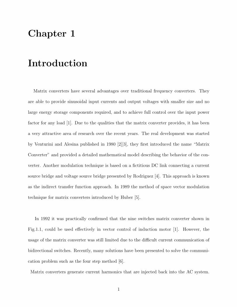
Matrix converters have several advantages over traditional frequency converters. They

are able to provide sinusoidal input currents and output voltages with smaller size and no

large energy storage components required, and to achieve full control over the input power

factor for any load [1]. Due to the qualities that the matrix converter provides, it has been

a very attractive area of research over the recent years. The real development was started

by Venturini and Alesina published in 1980 [2][3], they first introduced the name “Matrix

Converter” and provided a detailed mathematical model describing the behavior of the con-

verter. Another modulation technique is based on a fictitious DC link connecting a current

source bridge and voltage source bridge presented by Rodriguez [4]. This approach is known

as the indirect transfer function approach. In 1989 the method of space vector modulation

technique for matrix converters introduced by Huber [5].

In 1992 it was practically confirmed that the nine switches matrix converter shown in

Fig.1.1, could be used effectively in vector control of induction motor [1]. However, the

usage of the matrix converter was still limited due to the difficult current communication of

bidirectional switches. Recently, many solutions have been presented to solve the communi-

cation problem such as the four step method [6].

Matrix converters generate current harmonics that are injected back into the AC system.

1

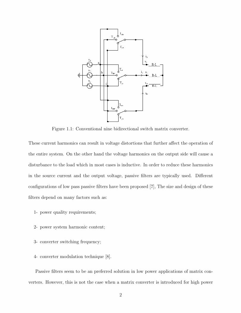
Figure 1.1: Conventional nine bidirectional switch matrix converter.

These current harmonics can result in voltage distortions that further affect the operation of

the entire system. On the other hand the voltage harmonics on the output side will cause a

disturbance to the load which in most cases is inductive. In order to reduce these harmonics

in the source current and the output voltage, passive filters are typically used. Different

configurations of low pass passive filters have been proposed [7], The size and design of these

filters depend on many factors such as:

1- power quality requirements;

2- power system harmonic content;

3- converter switching frequency;

4- converter modulation technique [8].

Passive filters seem to be an preferred solution in low power applications of matrix con-

verters. However, this is not the case when a matrix converter is introduced for high power

2

interfaces, the optimal design of the passive filter would be a major challenge.

The first high power matrix converter is introduced by Yaskawa for wind power appli-

cations [9], in which the modular concept is used to cope with the various demands in the

power grid. However, the modular concept is presented to be used in a very high voltages

applications such as wind mill and large problems. In this paper a hybrid matrix converter

will be introduced to operate at high power medium voltage demands. The proposed topol-

ogy employ a conventional nine-switch matrix converter coupled with shunt active filter

connected to the input side to reduce the source current harmonics, and series active filter

connected to the output side to reduce the output voltage harmonics. The two active filters

are connected through a small DC link capacitor.

The main matrix converter is modulated using the low frequency modulation algo-

rithm [10] to allow maximum voltage transfer ratio, and the active filters are controlled

based on the instantaneous reactive power theory [11] [12].

The thesis is organized as follows, The next chapter give a brief discussion about the

high frequency modulation techniques and explains the low frequency modulation technique.

The third chapter introduce the hybrid matrix converter and its operation. The fourth

chapter discuss the operation of hybrid matrix converter in abnormal conditions. The sixth

chapter discuss other conditioning method for hybrid matrix converter and introduce a new

conditioning technique to assess the evaluation of the previous methods.

3

Chapter 2

Background

This chapter aim to give a general description of the main features of matrix converter.

Matrix converter is a one stage AC-AC converter. It has several advantages over the conven-

tional AC-DC-AC converters such as sinusoidal input and output waveform, it has inhered

the bidirectional flow of power, and minimal energy storage requirements. Matrix converter

has also disadvantages. The maximum output voltage is 0.866% for sinusoidal input and

output waveform. It requires more semiconductor devices than the conventional AC-DC-AC

converters.

2.1 The Conventioanl Topology of Matrix Converter

The nine bidirectional switch three phase matrix converter is shown in Fig. 1.1. The input

terminal of the matrix converter is connected to a three phase voltage source. while the

output side is connected to a three phase load. The configuration of matrix converter theo-

retically assumes (512) switching configuration. However, if we take in the consideration the

constrains of the input being a voltage source and the output being a current source, such

that the input side of the matrix converter can not be short circuited and the output side

of the matrix converter can not be open circuited. This yield of only 27 feasible switching

combinations.

4

2.2 High Frequency Modulation Techniques of Matrix

Converter

In order to analysis the modulation techniques of matrix converter, its valid to consider ideal

switching and that the switching frequency is much higher that the input and the output

frequencies[15].

The input output relationships of voltages and currents are as follows.

vout = H · vin, (2.1)

iin = HT · iout, (2.2)

where vout is the output voltage vector [vu vv vw], vin is the input voltage vector [va vb vc],

iin is the input current vector [ia ib ic], and iout is the output current vector [iu iv iw].

H is the switching matrix of the matrix converter expressed as

H =

hau hbu hcu

hav hbv hcv

haw hbw hcw

. (2.3)

Each element in the transformation matrix (2.3) corresponds to one switching function for the

direction matrix converter. Considering that assumptions we made earlier and furthermore

neglecting all of the high frequency components we can replace the switching function in the

switching matrix in to the modulation function represented by the duty cycle.

The constrains of the input and the output sides of the matrix converter can be main-

tained via the following equations

5

hau + hbu + hcu = 1 (2.4)

hav + hbv + hcv = 1 (2.5)

haw + hbw + hcw = 1 (2.6)

The determination of any modulation strategy for the matrix converter is basically deter-

mining the appropriate duty cycle that the input-output relationships equ.( 2.1) and (2.2)

2.2.1 Alesina-Venturini 1981

The modulation of matrix converter can be stated as follows. Given a set of input voltages

and a set of output currents

vin = Vin

cos(ωit)

cos(ωit− 2π3 )

cos(ωit+ 2π3 )

. (2.7)

iout = Iout

cos(ωot+ φo)

cos(ωot− 2π3 + φo)

cos(ωot+ 2π3 + φo)

. (2.8)

find the modulation matrix H(t) such that

6

vout = qVin

cos(ωot)

cos(ωot− 2π3 )

cos(ωot+ 2π3 )

. (2.9)

and

iin = q cos(φo)Iout

cos(ωit+ φo)

cos(ωit− 2π3 + φo)

cos(ωit+ 2π3 + φo)

. (2.10)

where q is the voltage transfer ratio of the output and the input voltages. There are two

basic solution for this as shown below

The first method obtained by using the duty cycle of the matrix converter [16] represented

in the following equation

H1 =

1 + 2qcos(ωmt) 1 + 2qcos(ωmt− 2π

3 ) 1 + 2qcos(ωmt+ 2π3 )

1 + 2qcos(ωmt+ 2π3 )) 1 + 2qcos(ωmt) 1 + 2qcos(ωmt− 2π

3 )

1 + 2qcos(ωmt− 2π3 1 + 2qcos(ωmt+ 2π

3 )) 1 + 2qcos(ωmt))

. (2.11)

and

H2 =

1 + 2qcos(ωmt) 1 + 2qcos(ωmt− 2π

3 ) 1 + 2qcos(ωmt+ 2π3 )

1 + 2qcos(ωmt− 2π3 1 + 2qcos(ωmt+ 2π

3 )) 1 + 2qcos(ωmt))

1 + 2qcos(ωmt+ 2π3 )) 1 + 2qcos(ωmt) 1 + 2qcos(ωmt− 2π

3 )

. (2.12)

For H1 , ωm = ωo − ωi and for H2, ωm = −(ωo + ωi)

So for giving the same phase displacement at the input and the output ports φi = φo

7

gives (2.11), where φi = −φo gives (2.12). Combining the two solutions provides full control

over the input power factor.

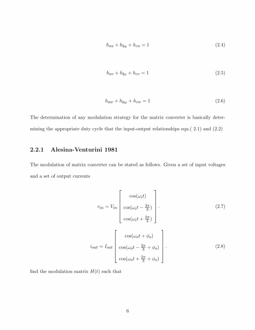
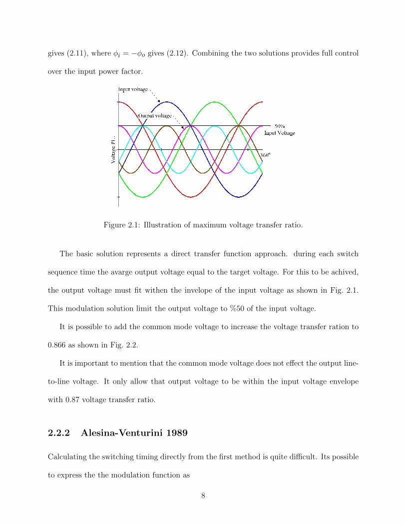
Figure 2.1: Illustration of maximum voltage transfer ratio.

The basic solution represents a direct transfer function approach. during each switch

sequence time the avarge output voltage equal to the target voltage. For this to be achived,

the output voltage must fit withen the invelope of the input voltage as shown in Fig. 2.1.

This modulation solution limit the output voltage to %50 of the input voltage.

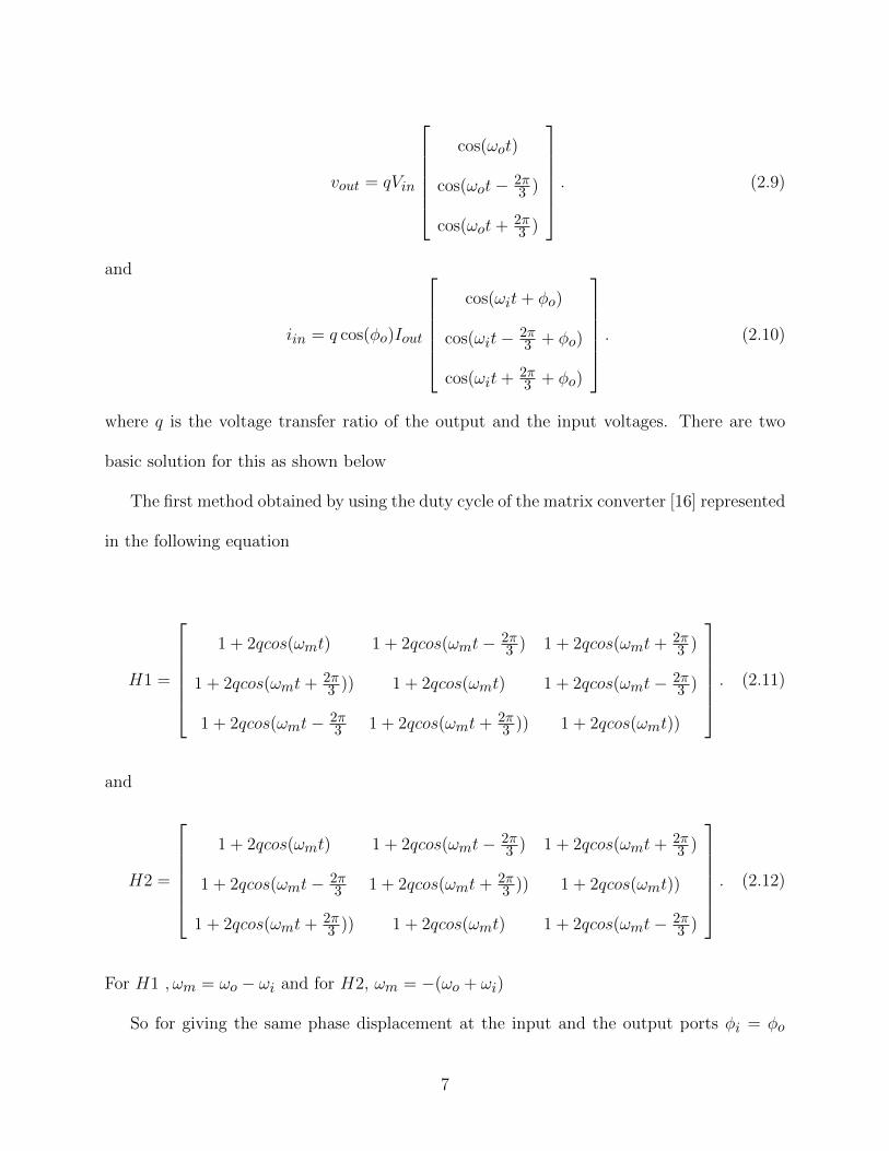
It is possible to add the common mode voltage to increase the voltage transfer ration to

0.866 as shown in Fig. 2.2.

It is important to mention that the common mode voltage does not effect the output line-

to-line voltage. It only allow that output voltage to be within the input voltage envelope

with 0.87 voltage transfer ratio.

2.2.2 Alesina-Venturini 1989

Calculating the switching timing directly from the first method is quite difficult. Its possible

to express the the modulation function as

8

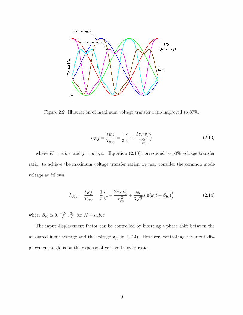
Figure 2.2: Illustration of maximum voltage transfer ratio improved to 87%.

hKj =tKjTseq

=1

3

(1 +

2vKvj

V 2in

)(2.13)

where K = a, b, c and j = u, v, w. Equation (2.13) correspond to 50% voltage transfer

ratio. to achieve the maximum voltage transfer ration we may consider the common mode

voltage as follows

hKj =tKjTseq

=1

3

(1 +

2vKvj

V 2in

+4q

3√

3sin(ωit+ βK)

)(2.14)

where βK is 0, −2π3 , 2π

3 for K = a, b, c

The input displacement factor can be controlled by inserting a phase shift between the

measured input voltage and the voltage vK in (2.14). However, controlling the input dis-

placement angle is on the expense of voltage transfer ratio.

9

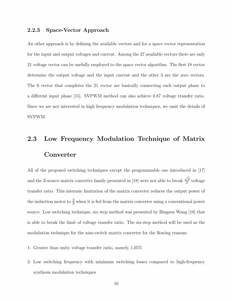
2.2.3 Space-Vector Approach

An other approach is by defining the available vectors and for a space vector representation

for the input and output voltages and current. Among the 27 available vectors there are only

21 voltage vector can be usefully employed to the space vector algorithm. The first 18 vector

determine the output voltage and the input current and the other 3 are the zero vectors.

The 6 vector that completes the 21 vector are basically connecting each output phase to

a different input phase [15]. SVPWM method can also achieve 0.87 voltage transfer ratio.

Since we are not interested in high frequency modulation techniques, we omit the details of

SVPWM.

2.3 Low Frequency Modulation Technique of Matrix

Converter

All of the proposed switching techniques except the programmable one introduced in [17]

and the Z-source matrix converter family presented in [18] were not able to break√

32 voltage

transfer ratio. This internsic limitation of the matrix converter reduces the output power of

the induction motor to 23 when it is fed from the matrix converter using a conventional power

source. Low switching technique, six step method was presented by Bingsen Wang [10] that

is able to break the limit of voltage transfer ratio. The six-step method will be used as the

modulation technique for the nine-switch matrix converter for the flowing reasons:

1- Greater than unity voltage transfer ratio, namely 1.05%

2- Low switching frequency with minimum switching losses compared to high-frequency

synthesis modulation techniques

10

3- Easy to control and implement.

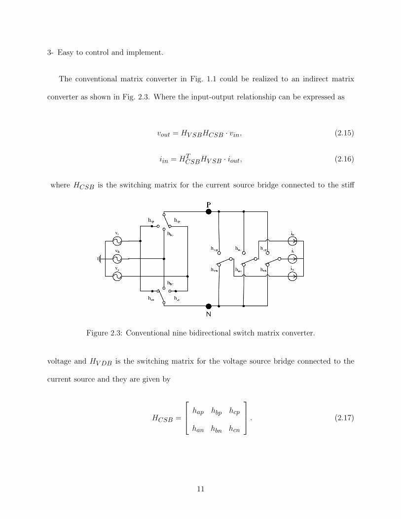
The conventional matrix converter in Fig. 1.1 could be realized to an indirect matrix

converter as shown in Fig. 2.3. Where the input-output relationship can be expressed as

vout = HV SBHCSB · vin, (2.15)

iin = HTCSBHV SB · iout, (2.16)

where HCSB is the switching matrix for the current source bridge connected to the stiff

Figure 2.3: Conventional nine bidirectional switch matrix converter.

voltage and HV DB is the switching matrix for the voltage source bridge connected to the

current source and they are given by

HCSB =

hap hbp hcp

han hbn hcn

. (2.17)

11

HCSB =

hup hun

hvp hvn

hwp hwn

. (2.18)

where

H = HCSB ·HCSB (2.19)

Any modulation technique that provides solution to the indirect realization of the matrix

converter can be applied to the direct matrix converter via (2.19). In our case the CSB will

be treated as a rectifier and the VSB will be treated a voltage source inverter, and both

converter are operating in full six-steps mode.

The switching signlas and the input-output voltage ans current are shown in 2.4.

Each element in the transformation matrix corresponds to one switching function for

the direction matrix converter. By an appropriate selection of the switching functions,

output voltages and the input currents similar to those of the voltage source inverter and

current source inverter, respectively, can be achieved. The resulting output voltages and

input currents for unity displacement factor operation at the input and output, and the

corresponding Fourier spectra are shown in Fig. 2.4 and 2.5, respectively.

The spctrum of the input current includes low frequency harmonic 5th and 7th. The load

voltage include the 5th and 7th as shown in Fig. 2.5.

The total harmonic distortion in both the input current and the output voltage is around

31%. The input current and output voltages waveform contain a low frequency harmonics,

and for high power application its difficult to design low pass filter that is able mitigate these

12

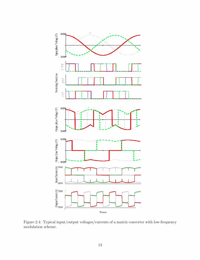
Figure 2.4: Typical input/output voltages/currents of a matrix converter with low-frequencymodulation scheme.

13

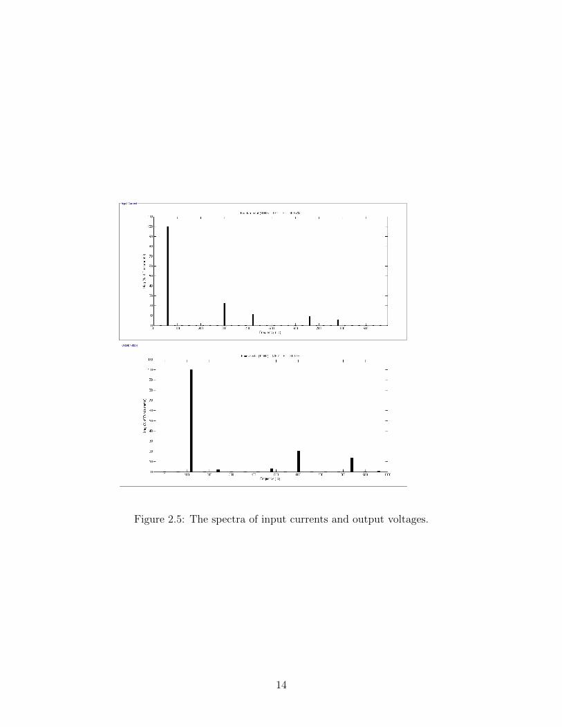
Figure 2.5: The spectra of input currents and output voltages.

14

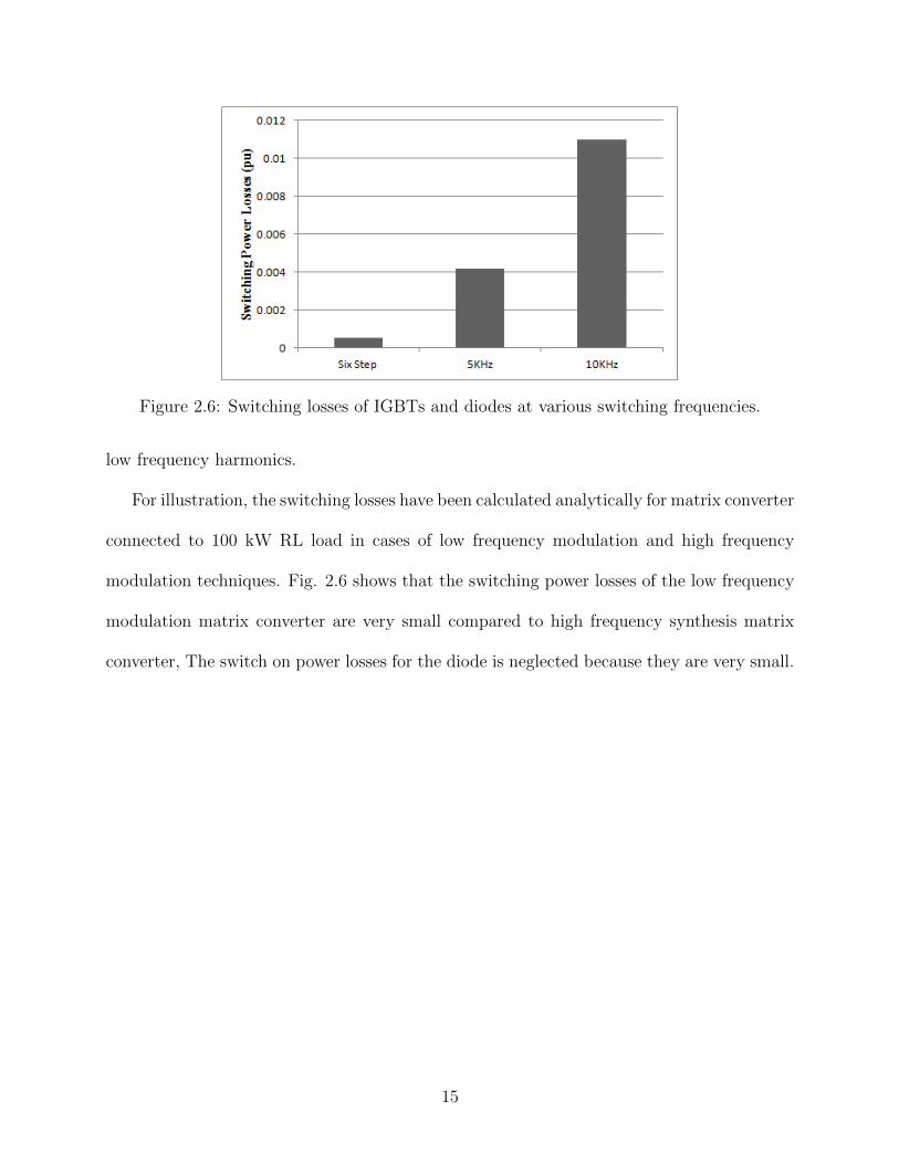
Figure 2.6: Switching losses of IGBTs and diodes at various switching frequencies.

low frequency harmonics.

For illustration, the switching losses have been calculated analytically for matrix converter

connected to 100 kW RL load in cases of low frequency modulation and high frequency

modulation techniques. Fig. 2.6 shows that the switching power losses of the low frequency

modulation matrix converter are very small compared to high frequency synthesis matrix

converter, The switch on power losses for the diode is neglected because they are very small.

15

Chapter 3

The Proposed Hybrid Matrix

Converter

Matrix converters would inject a significant amount of current harmonics and voltage har-

monics back in to the power source and the load, respectively, if filtering measures are not

properly implemented. These harmonics cause distortion and adversely impact the operation

of the whole system. The increasing demand for high power makes the conventional solution

of passive filters no longer sufficient to solve the power quality problem in matrix converters,

beside the other drawbacks of using bulky passive components such as, short life time, big

size, and high cost. This chapter presents a hybrid matrix converter for medium voltage high

power applications. By utilizing a low-frequency modulation techniques, combined with a

shunt active filter implemented to the input side of the matrix converter to eliminate current

harmonics and a series active filter is applied to the output side of the matrix converter

to eliminate the voltage harmonics. This approach is more efficient in terms of reducing

the total number of passive components used in the system, reducing the switching power

losses, and improving voltage transfer ratio. The explanation of predicting the compensa-

tion current and the compensation voltage waveforms is based on the instantaneous reactive

power theory. The feasibility and effectiveness proposed topology have been verified by the

simulation results.

16

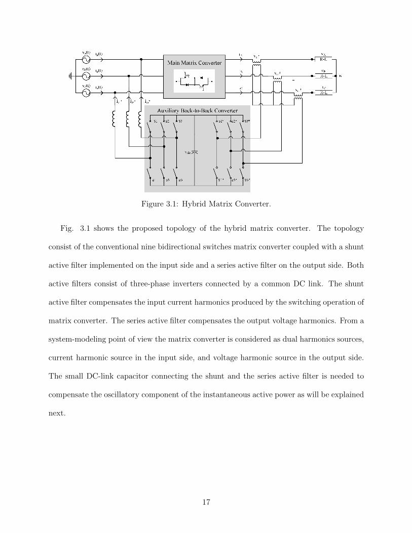
Figure 3.1: Hybrid Matrix Converter.

Fig. 3.1 shows the proposed topology of the hybrid matrix converter. The topology

consist of the conventional nine bidirectional switches matrix converter coupled with a shunt

active filter implemented on the input side and a series active filter on the output side. Both

active filters consist of three-phase inverters connected by a common DC link. The shunt

active filter compensates the input current harmonics produced by the switching operation of

matrix converter. The series active filter compensates the output voltage harmonics. From a

system-modeling point of view the matrix converter is considered as dual harmonics sources,

current harmonic source in the input side, and voltage harmonic source in the output side.

The small DC-link capacitor connecting the shunt and the series active filter is needed to

compensate the oscillatory component of the instantaneous active power as will be explained

next.

17

3.1 Active Filter Modulation

3.1.1 Input Current Conditioning

Considering the two waveforms at the input side, the three-phase input voltage is always

sinusoidal and the three-phase current is extremely distorted due to the switching action of

the matrix converter. The instantaneous three-phase active power at the input side p, can

be given by

pin = vin · vin, (3.1)

where ”·” denotes the internal product of the two vectors. Equation (3.1) can also expressed

in the conventional detention of power,

pin = iiva + ibvb + icvc. (3.2)

The instantaneous input reactive power vector of the three-phase system can be expressed

as

qin = vin × iin, (3.3)

where ”×” denotes the cross product of the voltage and current vectors. q can also be

18

expressed

qin =

qa

qb

qc

=

∣∣∣∣∣∣∣vb vc

ib ic

∣∣∣∣∣∣∣∣∣∣∣∣∣∣vc va

ic ia

∣∣∣∣∣∣∣∣∣∣∣∣∣∣va vb

ia ib

∣∣∣∣∣∣∣

, (3.4)

the norm of the reactive power vector is

qin = ‖qin‖ =√q2a + q2

b + q2c . (3.5)

We can decompose the source current into an active component iin−p, and reactive

component Iin−q in which

iin−p =

ia−p

ib−p

ic−p

=pin · vinvin · vin

, (3.6)

iin−q =

ia−q

ib−q

ia−q

=qin × vinvin · vin

, (3.7)

It is worth noting that the resultant current vector from the addition of the two cur-

rents iin−p and iin−q is always equal the source current iin. Another observation is that

the instantaneous power produced from vin · iin−p equal to the input power pin , and the

19

instantaneous power produced from vin · iin−q is always equal to zero. From this observation

we can tell that iin−q is not contributing to any power transmission from the source to the

load. In fact if the instantaneous reactive current is kept iin−q ≡ 0, the current iin will be

transmitting the same instantaneous active power pin with unity power factor.

Consequently, the instantaneous active power pin can be analyzed into two components,

pin = pin + pin, (3.8)

where pin is the direct component of the instantaneous active power and it represents the

energy flow in the direction from the source to the matrix converter. And pin represents

the oscillatory component of the instantaneous active power which is the energy exchanged

between the source and the matrix converter. By eliminating the current component that

produces pin, the source current will be sinusoidal. It is important to note that we do not

need an energy storing component to compensate the reactive power qin, because qin repre-

sents the energy exchange among the three-phases. While an we energy storing component

is required for compensating the oscillatory real power pin, because pin is the real power

exchanged between the source and the matrix converter.

Knowing this, we can generate the compensation current by selecting the appropriate

power portion to be eliminated. The three-phase compensation current could be expressed

as

i∗comp ==p∗comp · vinvin · vin

+q∗comp × vinvin · vin

, (3.9)

where p∗comp and q∗comp can be determined from pin and qin depending on the compen-

sation objectives.

20

3.1.2 Output Voltage Conditioning

The continuous current requirement of the matrix converter at the output side makes it

a perfect fit to apply the series active filter to compensate the output voltage harmonics.

By using the dual approach of the instantaneous reactive power theory we can define an

instantaneous active output power and instantaneous reactive output power as

pout = vout · iout, (3.10)

qout = vout × iout. (3.11)

In turn, we define the instantaneous active voltage vector Vout−p and instantaneous

reactive voltage vector Vout−q as

vout−p =

vA−p

vB−p

vC−p

=pout · i1outi1out · i1out

, (3.12)

vout−q =

vA−q

vB−q

vC−q

=qout × i1outi1out · i1out

, (3.13)

the superscript ”1” denotes the fundamental component of the output current. In most

cases, series active filters is used in applications where the current is sinusoidal. However,

this is not the case in the matrix converter and it requires further control effort to extract

the fundamental component of the output current.

21

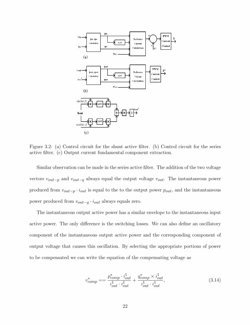
Figure 3.2: (a) Control circuit for the shunt active filter. (b) Control circuit for the seriesactive filter. (c) Output current fundamental component extraction.

Similar observation can be made in the series active filter. The addition of the two voltage

vectors vout−p and vout−q always equal the output voltage vout. The instantaneous power

produced from vout−p · iout is equal to the to the output power pout, and the instantaneous

power produced from vout−q · iout always equals zero.

The instantaneous output active power has a similar envelope to the instantaneous input

active power. The only difference is the switching losses. We can also define an oscillatory

component of the instantaneous output active power and the corresponding component of

output voltage that causes this oscillation. By selecting the appropriate portions of power

to be compensated we can write the equation of the compensating voltage as

v∗comp ==p∗comp · i1outi1out · i1out

+q∗comp × i1outi1out · i1out

, (3.14)

22

where p∗comp and q∗comp can be assigned from pout and qout according to our one’s compen-

sation objectives.

The control circuits of the two active filters are shown in Fig. 3.2(a) includes compu-

tational circuits for the instantaneous input reactive power qin, instantaneous oscillatory

component of the input active power pin, and instantaneous reactive component of the input

current iin−q, instantaneous oscillatory component of the input active current iin−p. circuit

Fig. 3.2(b) includes computational circuits for the instantaneous output reactive power qout,

instantaneous oscillatory component of the output active power pout, and instantaneous re-

active component of the output reactive voltage vout−q, instantaneous oscillatory component

of the output active voltage vout−p. Fig. 3.2(c) shows the fundamental component extraction

from the output current.

3.2 Simulation Results

A simulation model of the hybrid matrix converter as shown in Fig. 3.1 is build using

MATLAB Simulink. In the shunt active filter a hysteresis current controller is used to track

the instantaneous change of the inverter current and compare it back with the reference

current.

It is necessary to control the voltage of the DC link capacitor by adding the power

loss caused by the inverter switches. The active filter generates harmonics at its switching

frequency, and it is necessary to filter out these harmonic, typically, small coupling inductor

connected in series with the inverter output to eliminate these high frequency harmonics.

In our case the compensation powers are the reactive power and the oscillatory component

of the the active power. The compensation of reactive power will guarantee that there is

23

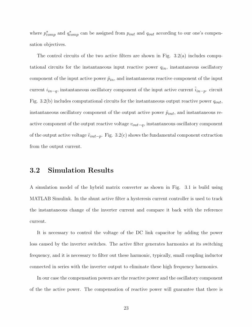
Figure 3.3: (a) Input compensation current injected by the shunt active filter. (b) Inputcurrent after using the shunt active filter. (c) Output compensation voltage injected by theseries active filter. (d) Output line voltage after using the series active filter.

no phase shift between the current and the voltage in the input and output side, and the

compensation of the oscillatory component of the active power will guarantee that the input

current and the output voltage are sinusoidal.

Fig.3.3 shows the input current and the output voltage after the compensation. in the

same phase with the input voltage which means that all the reactive power has been compen-

sated effectively. The compensation of the oscillatory component of the input active power

result in the sinusoidal shape of the input current. The same explanation can be made for

the output voltage.

24

3.3 conclusion and remarks

In this chapter, shunt and series active filters have been implemented on the input and the

output sides of the low-frequency modulated matrix converter, respectively. The analysis

of the input and output power shows that the instantaneous reactive power theory can

be applied in determining the compensation current of the input side and the compensation

voltage for the output side of the matrix converter. The proposed topology is very efficient in

medium voltage high power applications in which the conventional solution of passive filters is

not effective. The hybrid matrix converter reduces the size of energy storage components, and

provides higher reliability. The proposed topology could be utilized for mitigating the effect

of voltage sag, especially when the matrix converter is used to drive sensitive loads. More

detailed investigations will be reported in the future publications The DC link connecting

the two active filters can provide the same voltage stiffness in the AC-DC-AC back to back

inverters.

25

Chapter 4

Control Scheme of Hybrid Matrix

Converter Operating Under

Unbalanced Conditions

Hybrid matrix converters can potentially enable matrix converter in high-power applica-

tions that conventional matrix converters would not be able to attain. The hybrid matrix

converter consists a main matrix converter that processes the bulk power conversion and an

auxiliary back-back voltage source converter that improves the terminal power quality. Prior

simulation study has successfully demonstrated that the superior spectral performance can

be achieved. This chapter is focused on the control scheme of the hybrid matrix converter

operating under balanced and unbalanced conditions.

4.1 Unbalanced Voltage Source

In the previous chapter the assumption is made that the source voltage is balanced, meaning

the amplitudes of the three phase voltages are equal to each other and there is a 120o

phase shift among them. In case of unbalanced voltage source, further analysis needs to

be considered to obtain the correct compensation current for the input stage of the matrix

26

converter.

The unbalanced voltage source may include positive, negative, and zero sequence compo-

nents according to the symmetrical component theory. The symmetrical component trans-

formation is applied on both the input voltage and current to determine the sequence com-

ponents.

vin0

vin+

vin−

=1

3

1 1 1

1 α α2

1 α2 α

va

vb

vc

, (4.1)

The subscripts ”0”, ”+”, and ”-” correspond to the zero, positive, and negative sequences,

respectively. The complex number in the transformation matrix corresponds to the phase

shift in the three phase system, α = 1∠120o = ej2π3 ,

inin0

inin+

inin−

=1

3

1 1 1

1 α α2

1 α2 α

ina

inb

inc

, (4.2)

where ”n” denotes the harmonic component order.

The time domain equivalent voltage and current can be derived from the phasors given

by (4.1) and (4.2). By synthesizing the symmetrical components, the a−b−c input voltages

can be written as:

27

va =

vin0︷ ︸︸ ︷√2Vin0 sin(ωit+ φ0) +

vin+︷ ︸︸ ︷√2Vin+ sin(ωit+ φ+)

+

vin−︷ ︸︸ ︷√2Vin− sin(ωit+ φ−)

vb =√

2Vin0 sin(ωit+ φ0) +√

2Vin+ sin(ωit+ φ+ −2π

3)

+√

2Vin− sin(ωit+ φ− +2π

3)

vc =√

2Vin0 sin(ωit+ φ0) +√

2Vin+ sin(ωit+ φ+ +2π

3)

+√

2Vin− sin(ωit+ φ− −2π

3),

(4.3)

Similarly, the instantaneous input line currents are found to be

ina =

inin0︷ ︸︸ ︷√2Inin0 sin(ωit+ φ0) +

inin+︷ ︸︸ ︷√2Inin+ sin(ωit+ φ+)

+

inin−︷ ︸︸ ︷√2Inin− sin(ωit+ φ−)

inb =√

2Inin0 sin(ωit+ φ0) +√

2Inin+ sin(ωit+ φ+ −2π

3)

+√

2Inin− sin(ωit+ φ− +2π

3)

inc =√

2Inin0 sin(ωit+ φ0) +√

2Inin+ sin(ωit+ φ+ +2π

3)

+√

2Inin− sin(ωit+ φ− −2π

3),

(4.4)

The input current is the result of adding the results of all the time domain currents from

each harmonic.

ik =∞∑n=1

Ink k = (a, b, c). (4.5)

The above description allows us to analyze the three phase unbalanced system in to two

three phase balanced systems pulse zero sequence component. In the matrix converter case

28

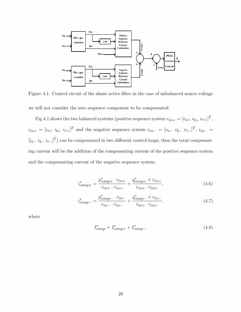
Figure 4.1: Control circuit of the shunt active filter in the case of unbalanced source voltage

we will not consider the zero sequence component to be compensated.

Fig.4.1 shows the two balanced systems (positive sequence system vin+ = [va+ vb+ vc+]T ,

iin+ = [ia+ ib+ ic+]T and the negative sequence system vin− = [va− vb− vc−]T , iin− =

[ia− ib− ic−]T ) can be compensated in two different control loops, then the total compensat-

ing current will be the addition of the compensating current of the positive sequence system

and the compensating current of the negative sequence system.

i∗comp+ =p∗comp+ · vin+

vin+ · vin++q∗comp+ × vin+

vin+ · vin+, (4.6)

i∗comp− =p∗comp− · vin−vin− · vin−

+q∗comp− × vin−vin+ · vin+

, (4.7)

where

I∗comp = I∗comp+ + I∗comp−. (4.8)

29

4.2 Unbalanced Load Current

In case of when different loads are connected to the matrix converter, each load will draw

a different amount of current leading to a linearly independent three phase output current.

The decomposition of the output voltage and current into it’s symmetrical component is as

follows:

vnout0

vnout+

vniout−

=1

3

1 1 1

1 α α2

1 α2 α

vnA

vnB

vnC

, (4.9)

i1in0

i1in+

i1in−

=1

3

1 1 1

1 α α2

1 α2 α

i1A

i1B

i1C

, (4.10)

The time domain equivalent voltage and current can be derived from the phasors given

by (4.9) and (4.10). By synthesizing the symmetrical components, the A − B − C voltage

and current can be written as:

30

vnA =

vnout0︷ ︸︸ ︷√2Vout0 sin(ωit+ φ0) +

vnout+︷ ︸︸ ︷√2Vout+ sin(ωit+ φ+)

+

vnout−︷ ︸︸ ︷√2Vout− sin(ωit+ φ−)

vnB =√

2Vout0 sin(ωit+ φ0) +√

2Vout+ sin(ωit+ φ+ −2π

3)

+√

2Vout− sin(ωit+ φ− +2π

3)

vnC =√

2Vout0 sin(ωit+ φ0) +√

2Vout+ sin(ωit+ φ+ +2π

3)

+√

2Vout− sin(ωit+ φ− −2π

3),

(4.11)

Similarly, the instantaneous line currents are found to be

i1A =

i1out0︷ ︸︸ ︷√2Inout0 sin(ωit+ φ0) +

i1out+︷ ︸︸ ︷√2Inout+ sin(ωit+ φ+)

+

i1out−︷ ︸︸ ︷√2Inout− sin(ωit+ φ−)

i1B =√

2Inout0 sin(ωit+ φ0) +√

2Inout+ sin(ωit+ φ+ −2π

3)

+√

2Inout− sin(ωit+ φ− +2π

3)

i1C =√

2Inout0 sin(ωit+ φ0) +√

2Inout+ sin(ωit+ φ+ +2π

3)

+√

2Inout− sin(ωit+ φ− −2π

3),

(4.12)

then the output voltage is the result of adding all the harmonics together

Vj =∞∑n=1

V nj j = (A,B,C). (4.13)

The same consideration of zero sequence voltages will be made here. The control process

is similar to the one we have in case of unbalanced source voltage, utilizing the output

31

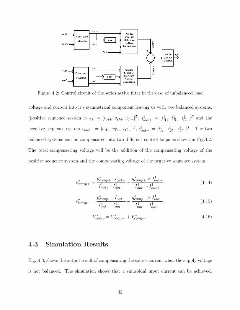
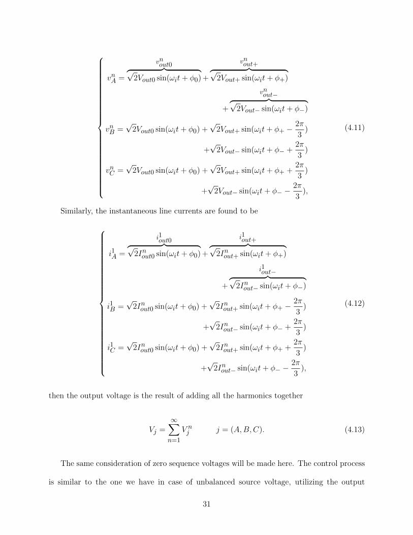
Figure 4.2: Control circuit of the series active filter in the case of unbalanced load

voltage and current into it’s symmetrical component leaving us with two balanced systems,

(positive sequence system vout+ = [vA+ vB+ vC+]T , i1out+ = [i1A+ i1B+ i1C+]T and the

negative sequence system vout− = [vA− vB− vC−]T , i1out− = [i1A− i1B− i1C−]T . The two

balanced systems can be compensated into two different control loops as shown in Fig.4.2.

The total compensating voltage will be the addition of the compensating voltage of the

positive sequence system and the compensating voltage of the negative sequence system.

v∗comp+ =p∗comp+ · I1

out+

I1out+ · I1

out+

+q∗comp+ × I1

out+

I1out+ · I1

out+

, (4.14)

v∗comp− =p∗comp− · I1

out−I1out− · I1

out−+q∗comp− × I1

out−I1out− · I1

out−, (4.15)

V ∗comp = V ∗comp+ + V ∗comp−. (4.16)

4.3 Simulation Results

Fig. 4.3, shows the output result of compensating the source current when the supply voltage

is not balanced. The simulation shows that a sinusoidal input current can be achieved.

32

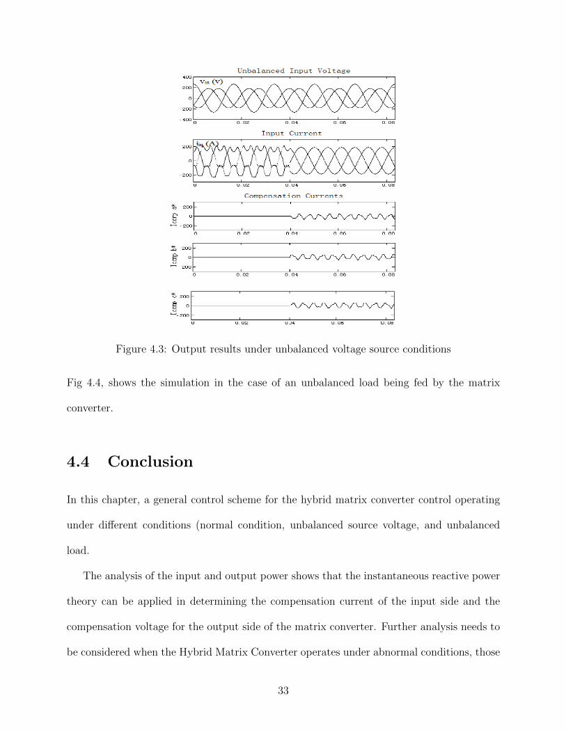
Figure 4.3: Output results under unbalanced voltage source conditions

Fig 4.4, shows the simulation in the case of an unbalanced load being fed by the matrix

converter.

4.4 Conclusion

In this chapter, a general control scheme for the hybrid matrix converter control operating

under different conditions (normal condition, unbalanced source voltage, and unbalanced

load.

The analysis of the input and output power shows that the instantaneous reactive power

theory can be applied in determining the compensation current of the input side and the

compensation voltage for the output side of the matrix converter. Further analysis needs to

be considered when the Hybrid Matrix Converter operates under abnormal conditions, those

33

Figure 4.4: Output results under unbalanced load conditions

analyses include the symmetrical component theory.

The proposed topology can be utilized for mitigating the effect of voltage sag, especially

when the matrix converter is used to drive sensitive loads.

34

Chapter 5

Critical Evaluation

This chapter is focused on conditioning the voltage and current waveform quality of a hybrid

matrix converter that consists of a conventional nine-switch matrix converter and a back-

to-back voltage source converter shoen in Fig. 3.1. Upon critical evaluation of the existing

methods for shunt and series compensation, the fundamental limitations for achieving su-

perior results have been identified. A new strategy based on power averaging for obtaining

the reference compensating current and voltage has been proposed. The effectiveness of

the proposed method has been evidenced by the simulation results for both the shunt and

series compensation with concurrent presence of the harmonic components in voltages and

currents.

Several AF control techniques have been presented in the literature [19][20][21]. Based

on the operating principle, these techniques can be categorized into two groups. The first

group of methods are based on instantaneous reactive power theory (IRPT) [22] and extract

the reactive component of the power and the oscillatory component of the real power. The

other methods are based on filtering techniques and extract the fundamental component

of the current or voltage such as notch filter and fast Fourier transform (FFT) methods

[23][24][25][26].

In this chapter different AF control strategies are presented and critically evaluated. The

limitations of the existing control approaches have been clearly identified.

35

In frequency-varying environment, the best solution is to use adaptive approach. How-

ever, notch filter is only able for harmonic detection and can not extract the reactive com-

ponents [26]. Further, such adaptive approaches might have convergence and robustness

problems [27]. Other filtering techniques such Fourier methods are widely used. Fast Fourier

transform requires high computational effort and discreet Fourier transform DFT requires

synchronization tool such phase-locked-loop (PLL). Furthermore, they share the same limita-

tion with adaptive notch filter of being unable to extract the reactive component. Therefore,

only the analysis of adaptive notch filter is presented in the this paper.

Instantaneous reactive power theory is a time domain method that based on the law of

conservation of energy.

It utilizes the concept that the non-active component of the voltage and current do not

contribute in any energy transfer from the source to the load. The Instantaneous reactive

power theory could undergo coordinate transformation to the synchronous reference frame.

This transformation changes the oscillating AC variables to a DC variables and the harmonics

appear in form of ripple in the DC signal. Although this approach provides extra filtering

to the system, its required synchronizing tool such as PLL.

The instantaneous reactive power theory seems to be a good solution in obtaining the

reactive components, it fails when both the current and the voltage contain harmonics. This

because of the overlap in the frequencies of the current and the voltage harmonics. Therefore,

it is incapable to obtain the correct compensating current or voltage when harmonics are

present in both the current and the voltage.

To address these limitations of the aforementioned methods, a new control strategy is

proposed. This proposed control method is able to effectively obtain the correct active

component of current or voltage in cases where both the current and the voltage are non-

36

sinusoidal and provide full control over the power factor.

5.1 Adaptive Notch Filter Method

Adaptive notch filtering is the technique that selectively extracts of a harmonic component

of certain frequency. It features very powerful qualities where elimination of certain har-

monics is required. Notch filter can estimate information embedded in the signal such as the

amplitude, frequency and phase angle, the signal frequency. The dynamic behavior of the

adaptive notch filter (ANF) can be characterized by the following deferential equations.

x′′

+ i2ω2x = 2ζω(u(t)− x′) (5.1)

ω′

= −γxω(u(t)− x′) (5.2)

where x is the integral of the fundamental component of the input signal u(t), ω is the

estimated frequency of the fundamental component; ζ and γ are adjustable real positive

parameters that determine the accuracy and convergence speed of the ANF; u(t) is the

signal from which the fundamental component is to be extracted. For a sinusoidal input

signal, the system described by (1) and (2) has a unique periodical orbit located at

x

x′

ω

=

−Aω1

cos(ω1t+ φ1)

A sin(ω1t+ φ1)

ω1

, (5.3)

where the estimated component of the frequency ω is identical to its actual value ω1, which is

mathematically explained in [26]. A detailed implementation of the ANF is shown in Fig.5.1.

37

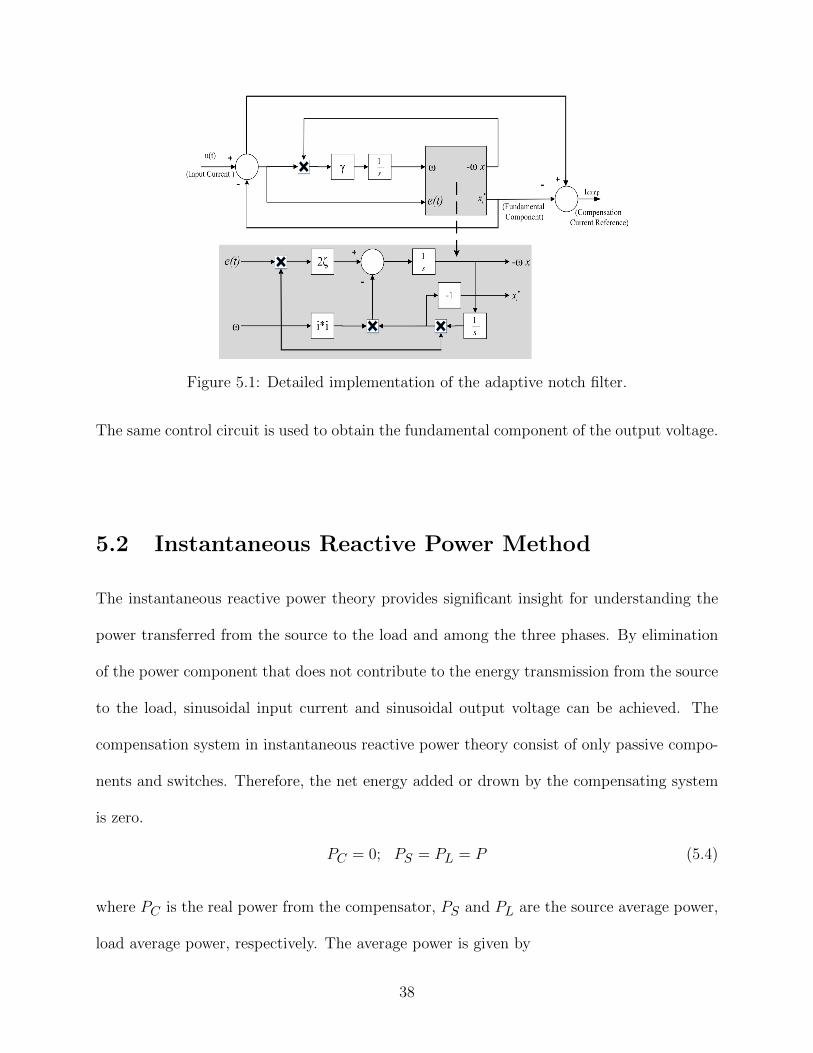
Figure 5.1: Detailed implementation of the adaptive notch filter.

The same control circuit is used to obtain the fundamental component of the output voltage.

5.2 Instantaneous Reactive Power Method

The instantaneous reactive power theory provides significant insight for understanding the

power transferred from the source to the load and among the three phases. By elimination

of the power component that does not contribute to the energy transmission from the source

to the load, sinusoidal input current and sinusoidal output voltage can be achieved. The

compensation system in instantaneous reactive power theory consist of only passive compo-

nents and switches. Therefore, the net energy added or drown by the compensating system

is zero.

PC = 0; PS = PL = P (5.4)

where PC is the real power from the compensator, PS and PL are the source average power,

load average power, respectively. The average power is given by

38

P = PX =1

TX

∫ t

t−TXp(τ)dτ. (5.5)

where TX denote the averaging interval that can be zero, one fundamental cycle, one-half

cycle, or multiple cycles, depending on compensation objectives and the passive components

energy storage capacity; p(τ) is the instantaneous real power.

The instantaneous reactive power theory work can be explained from early definition of

non-active current by Fryze [28].

ip(t) =(v, i)

(v, v)· v(t), iq(t) = i(t)− ip(t), (5.6)

where ip is the active current component, v(t) and i(t) is the reference voltage and current,

respectively, and iq is the non-active current component; (v, i) is the inner product of the

voltage and the current over the interval {t− TX , t} with respect to weighting factor equal

one, (v, v) is the inner product of the voltage and itself over the interval {t − TX , t} with

respect to weighting factor equal one. They can be expressed as follows

(v, i) = ‖v(t) · i(t)‖ =1

TX

∫ t

t−TXv(τ) · i(τ)dτ = P (5.7)

(v, v) = ‖v(t)‖2 =1

TX

∫ t

t−TXv2(τ)dτ = v2

rms (5.8)

5.2.1 Active Current on the Input Side

On the input side of the matrix converter the source voltage is sinusoidal and the source

current is not sinusoidal as it shown in Fig. 5.2(a). Therefore, they can be expressed by the

39

following equations

va(t) = VSf sin(ωit) (5.9)

ia(t) = ISf sin(ωit− α) + ISh sin(ωint+ βh) (5.10)

where VSf is the amplitude of the voltage fundamental component; ISf is the amplitude of

the current fundamental component; ISh is the amplitude of the h-th order harmonic, the

corresponding average power is

P =VSf ISf

2cosα (5.11)

It can be verified that the set of all harmonics in the current waveform ia(t) are orthogonal

with respect to the voltage va(t) over the interval of the integral. Therefore the corresponding

average power is only a result of the fundamental components of the current ia and the voltage

va(t).

Likewise, substituting (5.9) and (5.10) in (5.8) yields

va−rms =VSf√

2(5.12)

By substituting (5.7),(5.9),and (5.12)in (5.6), we can obtain the active current component

ip(t) = ISf cos(α) sin(ωt) (5.13)

This proves that the instantaneous reactive power theory is able to obtain the active com-

ponent of the current when the source voltage is sinusoidal and the source current contains

harmonics.

40

5.2.2 Active Voltage on the Output Side

On the output side of the matrix converter, both load voltage and current include harmonics

as shown in Fig. 5.2(a). Using a dual analogy to the active current defined in (6), we can

define the active component vp and the non-active component vq of the voltage as

vp(t) =(v, i)

(i, i)· i(t), vq(t) = v(t)− vp(t), (5.14)

where (i, i) is the inner product of the current and itself over the interval {t − TX , t} with

respect to weighting factor equal one. It is expressed as follows

(i, i) = ‖i(t)‖2 =1

TX

∫ t

t−TXi2(τ)dτ = i2rms (5.15)

The load voltage vA(t) and the load current iA(t) can be expressed by the following

equations

vA(t) = VLf sin(ωot) + VLh sin(ωoht+ βh) (5.16)

iA(t) = ILf sin(ωot− α) + ILh sin(ωont+ βh) (5.17)

where VLf is the amplitude of the voltage fundamental component; VLh is the amplitude of

the h-th order harmonic; ILf is the amplitude of the current fundamental component; ILh

is the amplitude of the h-th order harmonic, the corresponding average power is

P =VLf ILf

2cosα +

VLhILh2

cosαh (5.18)

and the corresponding rms current is

41

iA−rms =

√i2Lf + i2Lh

2(5.19)

By substituting (5.15), (5.17), and (5.18) in (5.14) we can obtain the active component

of the voltage

vp(t) =VLf ILf cosα + VLhILh cosαh

I2Lf + I2

Lh

(ILf sin(ωot) + ILh sin(ωont+ βh)) (5.20)

It is observed from (5.20) that the active component of the current is not sinusoidal.

Therefore, the instantaneous reactive power theory is not able to achieve a sinusoidal load

voltage. An FFT filter is used to obtain the fundamental component of the load current

before it is used in the control loop [29]. This limitation of the instantaneous reactive power

theory will be resolved by the proposed method in the next section.

By expanding the same approach for a three phase system we can define the compensation

current and the compensation voltage as follows

icomp =p · vinvin · vin

+q × vinvin · vin

(5.21)

vcomp =p · i1outi1out · i1out

+q × i1outi1out · i1out

(5.22)

where vin = [va vb vc]T is the input voltage vector; i1out = [iA iB iC ]T is the fundamental

output current vector; p is the oscillatory component of the real power; q is the reactive

power. The control block diagrams for the input current compensation and the output

voltage compensation are shown in Fig. 3(a). Both output current and voltage of the

42

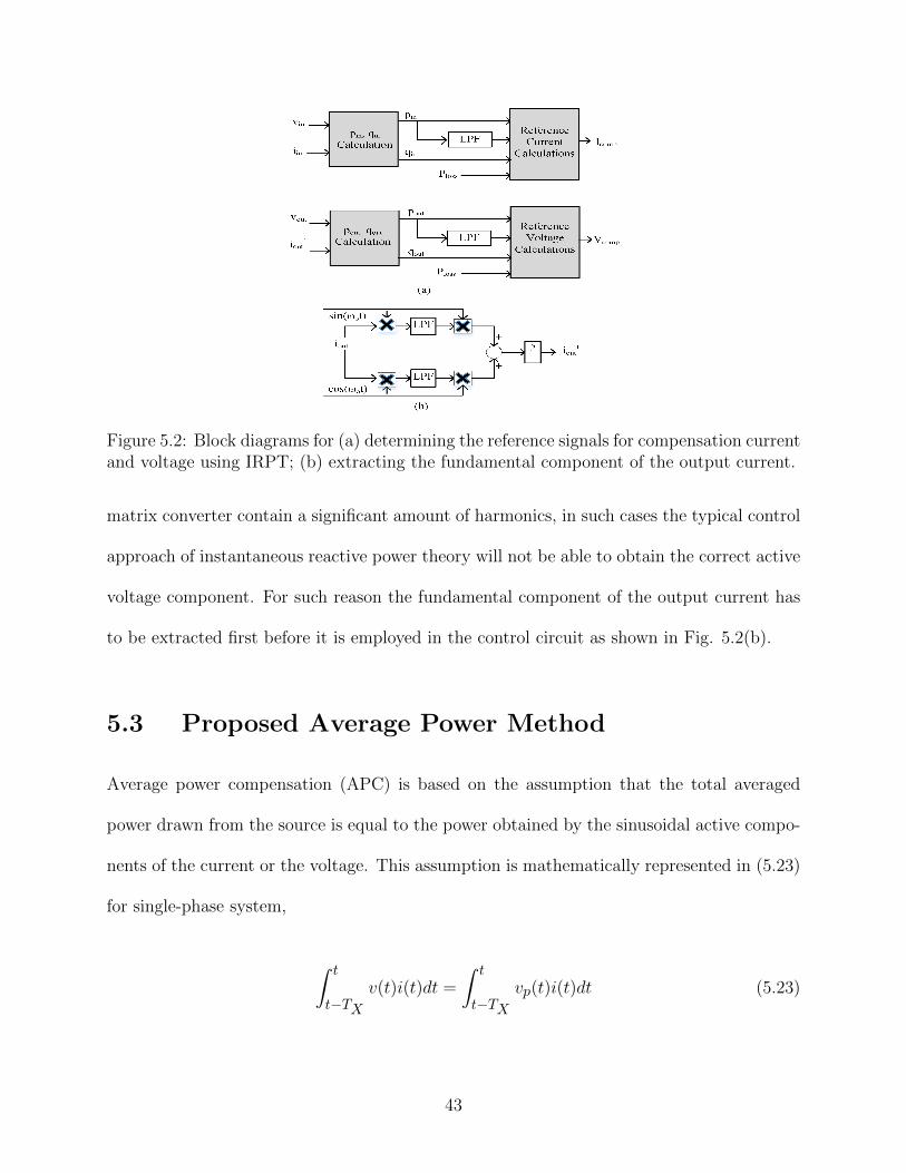
Figure 5.2: Block diagrams for (a) determining the reference signals for compensation currentand voltage using IRPT; (b) extracting the fundamental component of the output current.

matrix converter contain a significant amount of harmonics, in such cases the typical control

approach of instantaneous reactive power theory will not be able to obtain the correct active

voltage component. For such reason the fundamental component of the output current has

to be extracted first before it is employed in the control circuit as shown in Fig. 5.2(b).

5.3 Proposed Average Power Method

Average power compensation (APC) is based on the assumption that the total averaged

power drawn from the source is equal to the power obtained by the sinusoidal active compo-

nents of the current or the voltage. This assumption is mathematically represented in (5.23)

for single-phase system,

∫ t

t−TXv(t)i(t)dt =

∫ t

t−TXvp(t)i(t)dt (5.23)

43

where vp is the active component of the voltage. Assuming the the active component of the

voltage is sinusoidal, therefore,

vp(t) = A sin(ωot) (5.24)

We can estimate the amplitude of the active voltage component by substituting (5.16)

and (5.17) in (5.23), the amplitude A is determined by

A = vaf cos(α) +vahiah cos(αh)

iaf(5.25)

From the active voltage amplitude in (5.25), it can be observed that the active component

of the current vp is not equal to the fundamental component, which is the fundamental reason

that the ANF methods will not achieve maximum power transfer. A dual approach can be

easily implemented to obtain the active component of the input current. The block diagram

of averaged power method for the input current and the output voltage compensation are

shown in Fig. 5.3(a) and (b), respectively.

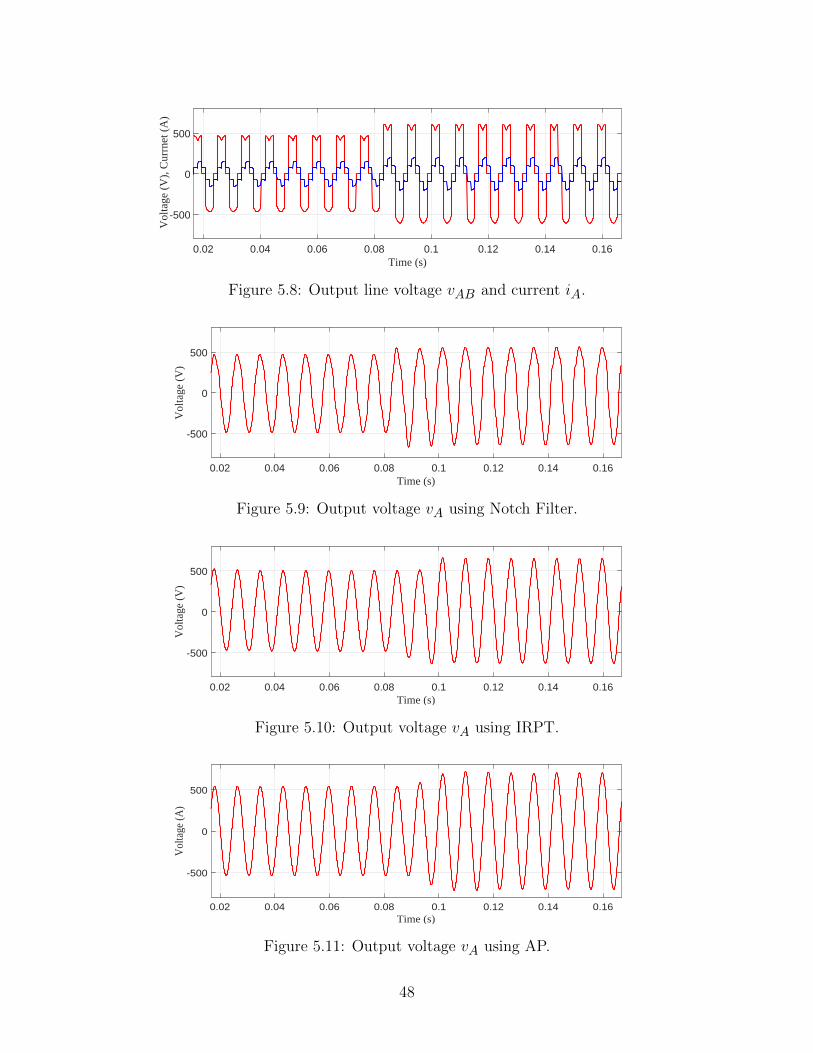
5.4 Simulation Results and Evaluation

To evaluate the performance of the presented methods detailed simulation models have been

constructed based on the three phase hybrid matrix converter shown in Fig. ??. In each

simulation model the control method is applied to compensate both the input current and

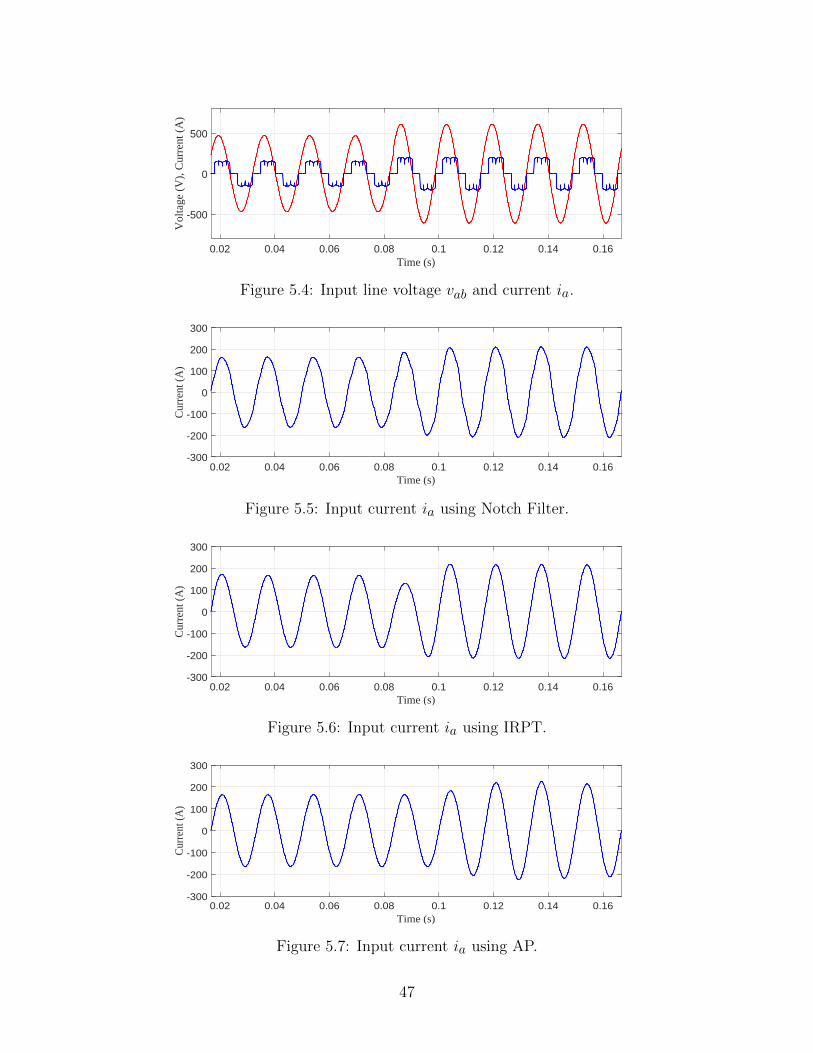
the output voltage harmonics. The typical input and output current and voltage waveforms

of the main matrix converter are shown in Fig. 5(a) and (b). Fig. 8(c) shows the input

source current after compensation using adaptive notch filter method, by which the funda-

mental component of the input current is calculated. The harmonic content is obtained by

44

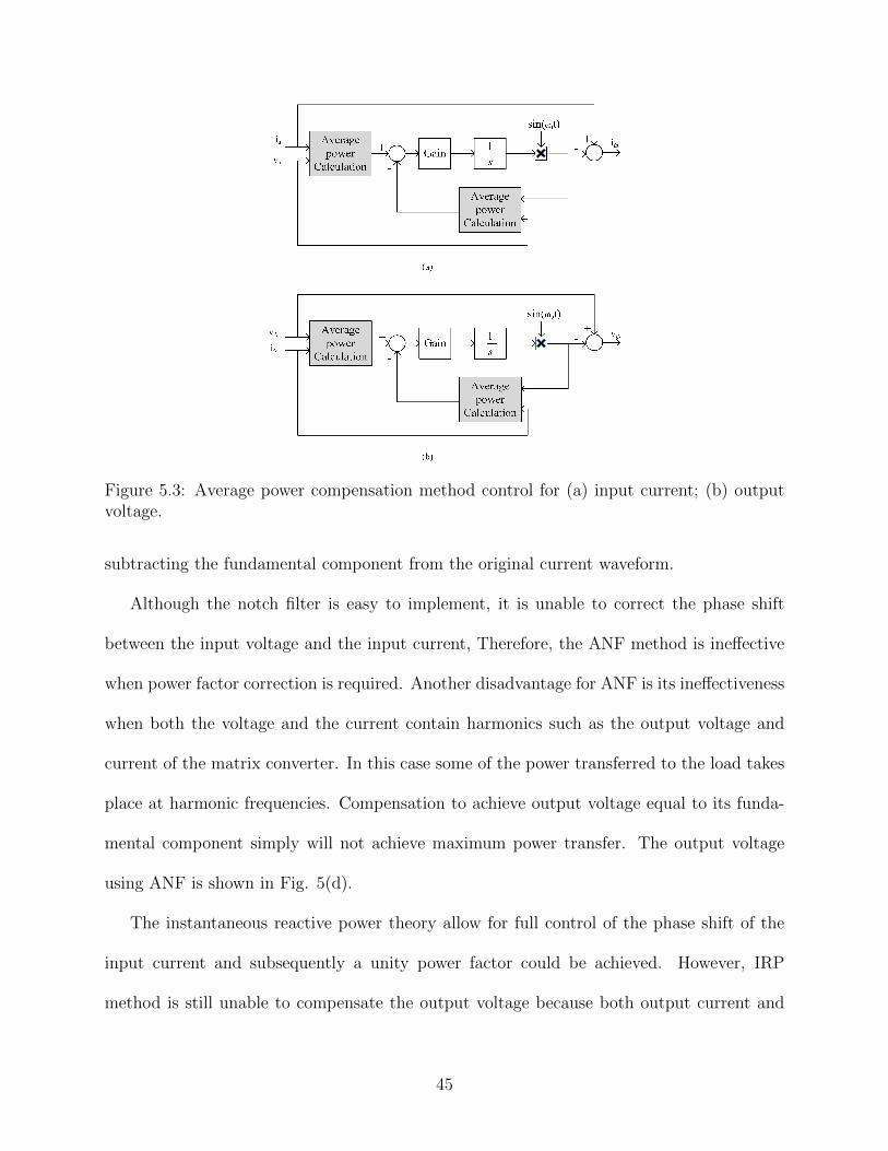
Figure 5.3: Average power compensation method control for (a) input current; (b) outputvoltage.

subtracting the fundamental component from the original current waveform.

Although the notch filter is easy to implement, it is unable to correct the phase shift

between the input voltage and the input current, Therefore, the ANF method is ineffective

when power factor correction is required. Another disadvantage for ANF is its ineffectiveness

when both the voltage and the current contain harmonics such as the output voltage and

current of the matrix converter. In this case some of the power transferred to the load takes

place at harmonic frequencies. Compensation to achieve output voltage equal to its funda-

mental component simply will not achieve maximum power transfer. The output voltage

using ANF is shown in Fig. 5(d).

The instantaneous reactive power theory allow for full control of the phase shift of the

input current and subsequently a unity power factor could be achieved. However, IRP

method is still unable to compensate the output voltage because both output current and

45

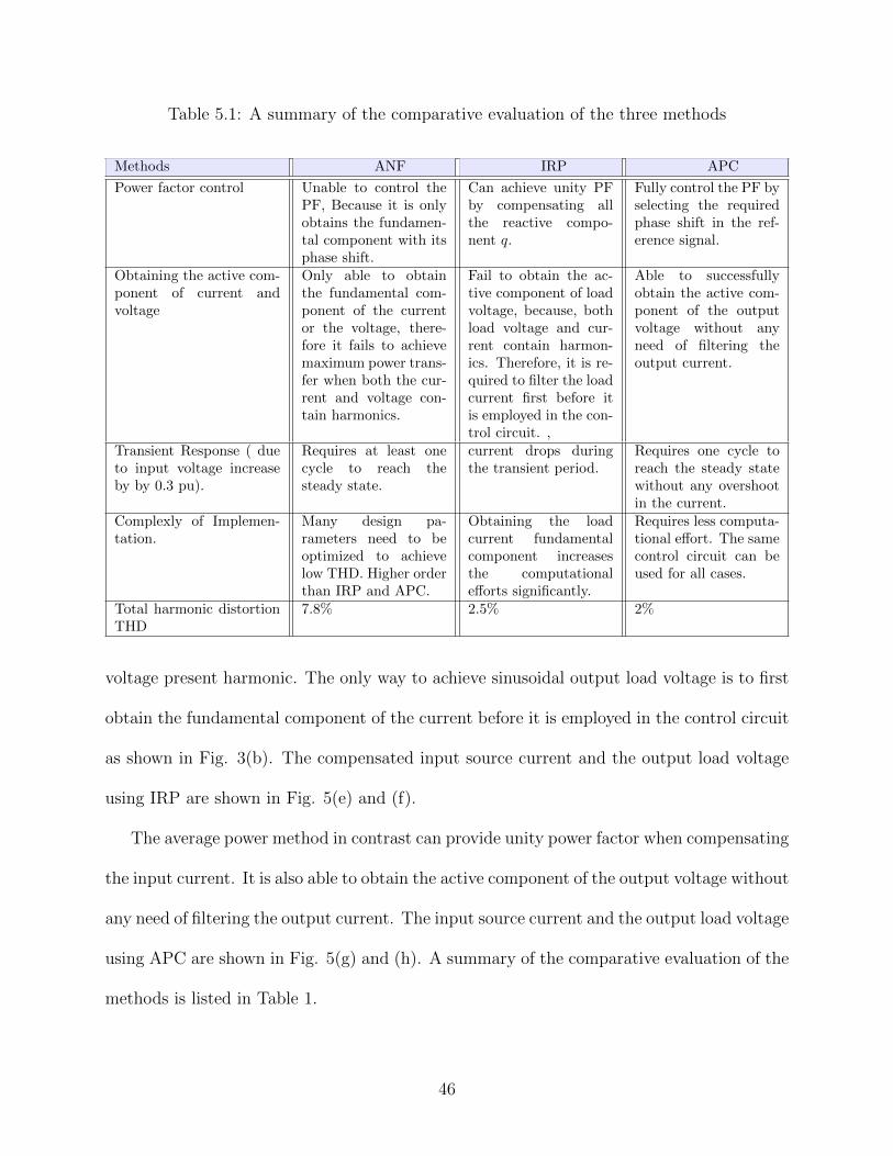
Table 5.1: A summary of the comparative evaluation of the three methods

Methods ANF IRP APC

Power factor control Unable to control thePF, Because it is onlyobtains the fundamen-tal component with itsphase shift.

Can achieve unity PFby compensating allthe reactive compo-nent q.

Fully control the PF byselecting the requiredphase shift in the ref-erence signal.

Obtaining the active com-ponent of current andvoltage

Only able to obtainthe fundamental com-ponent of the currentor the voltage, there-fore it fails to achievemaximum power trans-fer when both the cur-rent and voltage con-tain harmonics.

Fail to obtain the ac-tive component of loadvoltage, because, bothload voltage and cur-rent contain harmon-ics. Therefore, it is re-quired to filter the loadcurrent first before itis employed in the con-trol circuit. ,

Able to successfullyobtain the active com-ponent of the outputvoltage without anyneed of filtering theoutput current.

Transient Response ( dueto input voltage increaseby by 0.3 pu).

Requires at least onecycle to reach thesteady state.

current drops duringthe transient period.

Requires one cycle toreach the steady statewithout any overshootin the current.

Complexly of Implemen-tation.

Many design pa-rameters need to beoptimized to achievelow THD. Higher orderthan IRP and APC.

Obtaining the loadcurrent fundamentalcomponent increasesthe computationalefforts significantly.

Requires less computa-tional effort. The samecontrol circuit can beused for all cases.

Total harmonic distortionTHD

7.8% 2.5% 2%

voltage present harmonic. The only way to achieve sinusoidal output load voltage is to first

obtain the fundamental component of the current before it is employed in the control circuit

as shown in Fig. 3(b). The compensated input source current and the output load voltage

using IRP are shown in Fig. 5(e) and (f).

The average power method in contrast can provide unity power factor when compensating

the input current. It is also able to obtain the active component of the output voltage without

any need of filtering the output current. The input source current and the output load voltage

using APC are shown in Fig. 5(g) and (h). A summary of the comparative evaluation of the

methods is listed in Table 1.

46

Time (s)0.02 0.04 0.06 0.08 0.1 0.12 0.14 0.16

Vol

tage

(V

), C

urre

nt (

A)

-500

0

500

Figure 5.4: Input line voltage vab and current ia.

Time (s)0.02 0.04 0.06 0.08 0.1 0.12 0.14 0.16

Cur

rent

(A

)

-300

-200

-100

0

100

200

300

Figure 5.5: Input current ia using Notch Filter.

Time (s)0.02 0.04 0.06 0.08 0.1 0.12 0.14 0.16

Cur

rent

(A

)

-300

-200

-100

0

100

200

300

Figure 5.6: Input current ia using IRPT.

Time (s)0.02 0.04 0.06 0.08 0.1 0.12 0.14 0.16

Cur

rent

(A)

-300

-200

-100

0

100

200

300

Figure 5.7: Input current ia using AP.

47

Time (s)0.02 0.04 0.06 0.08 0.1 0.12 0.14 0.16

Vol

tage

(V

), C

urrn

et (

A)

-500

0

500

Figure 5.8: Output line voltage vAB and current iA.

Time (s)0.02 0.04 0.06 0.08 0.1 0.12 0.14 0.16

Vol

tage

(V

)

-500

0

500

Figure 5.9: Output voltage vA using Notch Filter.

Time (s)0.02 0.04 0.06 0.08 0.1 0.12 0.14 0.16

Vol

tage

(V

)

-500

0

500

Figure 5.10: Output voltage vA using IRPT.

Time (s)0.02 0.04 0.06 0.08 0.1 0.12 0.14 0.16

Vol

tage

(A)

-500

0

500

Figure 5.11: Output voltage vA using AP.

48

5.5 Conclusion

This paper has presented the preliminary results for the evaluation of existing approaches to

shunt and series conditioning of the currents and voltages. The critically evaluated methods

are based on either instantaneous reactive power theory or fast Fourier transform. The

main limitation for IRPT based method lies in its ineffectiveness when the harmonics are

concurrently present in voltage and current while the limitation for FFT based method is its

inability to compensate the fundamental component. To address the limitations associated

with the existing methods, a new method based on power averaging has been proposed. The

effectiveness of the proposed method has been verified by the simulation results obtained from

a detailed MathCAD/Simulink model. Furthermore, experimental work has been planned

and the experimental results will be included in the final manuscript.

49

BIBLIOGRAPHY

50

BIBLIOGRAPHY

[1] Wheeler, P.W.; Rodriguez, J.; Clare, J.C.; Empringham, L.; Weinstein, A.,“Matrixconverters: a technology review,” IEEE Transactions on Industrial Electronics, vol.49,no.2, pp.276,288, Apr 2002

[2] M. Venturini, “A new sine wave in sine wave out, conversion technique which eliminatesreactive elements”, Proc. POWERCON 7, pp.E31-E315 1980

[3] M. Venturini and A. Alesina, “The generalized transformer: A new bidirectional sinu-soidal waveform frequency converter with continuously adjustable input power factor”,Proc. IEEE PESC’,80, pp.242 -252 1980

[4] J. Rodriguez, “A new control technique for AC-AC converters”, Proc. IFAC Controlin Power Electronics and Electrical Drives Conf., pp.203-208 1983

[5] L. Huber and D. Borojevic, “Space vector modulated three-phase to three-phase matrixconverter with input power factor correction”, IEEE Trans. Ind. Applicat., vol. 31,pp.1234 -1246 1995

[6] Burany, N., “Safe control of four-quadrant switches,” Industry Applications SocietyAnnual Meeting, 1989., Conference Record of the 1989 IEEE , vol., no., pp.1190,1194vol.1, 1-5 Oct. 1989

[7] A. Popovici, V. Popescu, M. Babaita, D. Lascu, D.Negoitescu, “Modeling, Simulationand Design of Input Filter for Matrix Converters”,2005 WSEAS Int. Conf. on DYNAM-ICAL SYSTEMS and CONTROL, Venice, Italy, November 2-4, 2005 (pp439-444)

[8] Empringham, L.; Kolar, J.W.; Rodriguez, J.; Wheeler, P.W.; Clare, J.C., “Technolog-ical Issues and Industrial Application of Matrix Converters: A Review,” IEEE Trans-actions on Industrial Electronics , vol.60, no.10, pp.4260,4271, Oct. 2013

[9] Jun Kang; Takada, Noriyuki; Yamamoto, E.; Watanabe, E., “High power matrix con-verter for wind power generation applications,” Power Electronics and ECCE Asia(ICPE - ECCE), 2011 IEEE 8th International Conference on , vol., no., pp.1331,1336,May 30 2011-June 3 2011

51

[10] Bingsen Wang; Venkataramanan, G., “Six Step Modulation of Matrix Converter withIncreased Voltage Transfer Ratio,” Power Electronics Specialists Conference, 2006.PESC ’06. 37th IEEE , vol., no., pp.1,7, 18-22 June 2006

[11] H. Akagi, Y. Kanazawa, and A. Nabae, “Instantaneous reactive power compensatorscomprising switching devices without energy storage components”, IEEE Trans. Ind.Appl., vol. 20, pp.625 -630 1984

[12] Fang Zheng Peng; Jih-Sheng Lai, “Generalized instantaneous reactive power theoryfor three-phase power systems,” IEEE Transactions on Instrumentation and Measure-ment,, vol.45, no.1, pp.293,297, Feb 1996

[13] P. D. Ziogas, S. I. Khan, and M. H. Rashid,“Analysis and design of forced commutatedcycloconverter structures with improved transfer characteristics,” IEEE Transactionson Industrial Electronics, vol. IE- 33, no. 3, pp. 271, 1986.

[14] Baoming Ge; Qin Lei; Wei Qian; Fang Zheng Peng, “A Family of Z-Source MatrixConverters,” , IEEE Transactions on Industrial Electronics , vol.59, no.1, pp.35,46,Jan. 2012

[15] D. Casadei, G. Serra, A. Tani and L. Zarri, ”Matrix converter modulation strategies:a new general approach based on space-vector representation of the switch state,” inIEEE Transactions on Industrial Electronics, vol. 49, no. 2, pp. 370-381, Apr 2002.

[16] A. Alesina and M. Venturini, ”Solid-state power conversion: A Fourier analysis ap-proach to generalized transformer synthesis”, IEEE Trans. Circuits Syst., vol. CAS-28,pp. 319-330, 1981

[17] P. D. Ziogas, S. I. Khan, and M. H. Rashid,“Analysis and design of forced commutatedcycloconverter structures with improved transfer characteristics,” IEEE Transactionson Industrial Electronics, vol. IE- 33, no. 3, pp. 271, 1986.

[18] Baoming Ge; Qin Lei; Wei Qian; Fang Zheng Peng, “A Family of Z-Source MatrixConverters,”IEEE Transactions on Industrial Electronic, vol.59, no.1, pp.35,46, Jan.2012

[19] H. Akagi, Y. Kanazawa, and A. Nabae, “Instantaneous reactive power compensatorscomprising switching devices without energy storage components,” IEEE Transactionson Industry Applications, vol. IA-20, no. 3, pp. 625-630, 1984.

52

[20] F. Z. Peng, H. Akagi, and A. Nabae, “A new approach to harmonic compensationin power systems,” in Record of the IEEE Industry Applications Society 23rd AnnualMeeting, Pittsburgh, PA, Oct. 2-7, 1988, pp. 874-880.

[21] F. Z. Peng and J. S. Lai, “Generalized instantaneous reactive power theory for three-phase power systems,” IEEE Transactions on Instrumentation and Measurement, vol.45, no. 1, pp.293-297, 1996.

[22] F. Z. Peng, H. Akagi, and A. Nabae, “A new approach to harmonic compensationin power systems-a combined system of shunt passive and series active filters,” IEEETransactions on Industry Applications, vol. 26, no. 6, pp. 983-990, 1990.

[23] D. Yazdani, A. Bakhshai, G. Joos, and M. Mojiri, “A real-time selective harmonicextraction approach based on adaptive notch filtering,” in Proceedings of IEEE Inter-national Symposium on Industrial Electronics, Jun. 30 - Jul. 2, 2008, pp. 226-230.

[24] D. Yazdani, A. Bakhshai, G. Joos and M. Mojiri,“A Real-Time Three-Phase Selective-Harmonic-Extraction Approach for Grid-Connected Converters” IEEE Transactionson Industrial Electronics, vol. 56, no. 10, pp. 4097-4106, Oct. 2009.

[25] E. Lavopa, P. Zanchetta, M. Sumner, and F. Cupertino, “Real-time estimation offundamental frequency and harmonics for active shunt power filters in aircraft electricalsystems,” IEEE Transactions on Industrial Electronics, vol. 56, no. 8, pp. 2875-2884,2009.

[26] M. Mojiri, and A. R. Bakhshai, “An adaptive notch filter for frequency estimation ofa periodic signal,” in IEEE Transactions on Automatic Control, vol. 49, no. 2, pp.314-318, 2004.

[27] L. Asiminoaei, F. Blaabjerg, and S. Hansen, “Detection is key?Harmonic detectionmethods for active power filter applications” IEEE Ind. Appl. Mag., vol. 13, no. 4, pp.22?33, Jul./Aug. 2007.

[28] S. Fryze, ?Active, “Reactive, and Apparent Power in Non-Sinusoidal Systems,”Przeglad Elektrot, no. 7, pp. 193-203, 1931. (in Polish)

[29] P. Salmeron and S. P. Litran,“Improvement of the Electric Power Quality Using SeriesActive and Shunt Passive Filters” Transactions on Power Delivery, vol. 25, no. 2, pp.1058-1067, April 2010.

53