shumway 2001

Forecasting Bankruptcy More Accurately: A Simple Hazard ModelAuthor(s): Tyler ShumwayReviewed work(s):Source: The Journal of Business, Vol. 74, No. 1 (January 2001), pp. 101-124Published by: The University of Chicago PressStable URL: http://www.jstor.org/stable/10.1086/209665 .Accessed: 27/04/2012 07:48

Your use of the JSTOR archive indicates your acceptance of the Terms & Conditions of Use, available at .http://www.jstor.org/page/info/about/policies/terms.jsp

JSTOR is a not-for-profit service that helps scholars, researchers, and students discover, use, and build upon a wide range ofcontent in a trusted digital archive. We use information technology and tools to increase productivity and facilitate new formsof scholarship. For more information about JSTOR, please contact [email protected].

The University of Chicago Press is collaborating with JSTOR to digitize, preserve and extend access to TheJournal of Business.

http://www.jstor.org

http://www.jstor.org/action/showPublisher?publisherCode=ucpress

http://www.jstor.org/stable/10.1086/209665?origin=JSTOR-pdf

http://www.jstor.org/page/info/about/policies/terms.jsp

I argue that hazardmodels are more appro-priate than single-period models for fore-casting bankruptcy.Single-period modelsare inconsistent, whilehazard models produceconsistent estimates. Idescribe a simple tech-nique for estimating adiscrete-time hazardmodel. I find thatabout half of the ac-counting ratios thathave been used in pre-vious models are notstatistically signifi-cant. Moreover, marketsize, past stock returns,and idiosyncratic re-turns variability are allstrongly related tobankruptcy. I proposea model that uses bothaccounting ratios andmarket-driven variablesto produce out-of-sam-ple forecasts that aremore accurate thanthose of alternativemodels.

Tyler ShumwayUniversity of Michigan

Forecasting Bankruptcy MoreAccurately: A Simple HazardModel*

I. Introduction

Economists and accountants have been forecast-ing bankruptcy for decades (see Altman 1993 fora survey). Most researchers have estimated sin-gle-period classification models, which I refer toas static models, with multiple-period bankruptcydata. By ignoring the fact that firms changethrough time, static models produce bankruptcyprobabilities that are biased and inconsistent esti-mates of the probabilities that they approximate.Test statistics that are based on static models giveincorrect inferences. I propose a hazard modelthat is simple to estimate, consistent, and accu-rate.

Static models are inappropriate for forecastingbankruptcy because of the nature of bankruptcydata. Since bankruptcy occurs infrequently, fore-casters use samples that span several years to es-timate their models.1 The characteristics of mostfirms change from year to year. However, staticmodels can only consider one set of explanatoryvariables for each firm. Researchers who apply

* I thank Chris Acito, Steve Boyce, John Cochrane, GeorgeConstantinides, Dennis Capozza, Kathryn Clark, Josh Coval,Eugene Fama, Chris Geczy, Paul Gompers, Steve Kaplan,Michael Parzen, Burt Porter, Ross Stevens, Kelly Welch, SvenWilson, Arnold Zellner, Luigi Zingales, Mark Zmijewski, ananonymous referee, and seminar participants at the Universityof Chicago, Brigham Young University, and the University ofMichigan for suggestions.

1. For example, Altman’s (1968) original bankruptcy sam-ple spans 20 years. The sample used in this article includesbankruptcies observed over 31 years.

(Journal of Business, 2001, vol. 74, no. 1) 2001 by The University of Chicago. All rights reserved.0021-9398/2001/7401-0005$02.50

101

102 Journal of Business

static models to bankruptcy have to select when to observe each firm’scharacteristics. Most forecasters choose to observe each bankruptfirm’s data in the year before bankruptcy. They ignore data on healthyfirms that eventually go bankrupt. By choosing when to observe eachfirm’s characteristics arbitrarily, forecasters who use static models in-troduce an unnecessary selection bias into their estimates.

I develop a simple hazard model that uses all available informationto determine each firm’s bankruptcy risk at each point in time (seeKiefer 1988; Lancaster 1990). While static models produce biased andinconsistent bankruptcy probability estimates, the hazard model pro-posed here is consistent in general and unbiased in some cases. Estimat-ing hazard models with the accounting variables used previously byAltman (1968) and Zmijewski (1984) reveals that half of these vari-ables are statistically unrelated to bankruptcy probability. I develop anew bankruptcy model that uses three market-driven variables to iden-tify failing firms. My new model outperforms alternative models inout-of-sample forecasts.

A. Advantages of Hazard Models

Hazard models resolve the problems of static models by explicitly ac-counting for time. The dependent variable in a hazard model is the timespent by a firm in the healthy group. When firms leave the healthygroup for some reason other than bankruptcy (e.g., merger), they areconsidered censored, or no longer observed. Static models simply con-sider such firms healthy. In a hazard model, a firm’s risk for bankruptcychanges through time, and its health is a function of its latest financialdata and its age. The bankruptcy probability that a static model assignsto a firm does not vary with time.

In econometric terms, there are three reasons to prefer hazard modelsfor forecasting bankruptcy. The first reason is that static models fail tocontrol for each firm’s period at risk. When sampling periods are long,it is important to control for the fact that some firms file for bankruptcyafter many years of being at risk while other firms fail in their firstyear. Static models do not adjust for period at risk, but hazard modelsadjust for it automatically. The selection bias inherent in static bank-ruptcy models is a result of the failure to correct for period at risk.

The second reason to prefer hazard models is that they incorporatetime-varying covariates, or explanatory variables that change with time.If a firm deteriorates before bankruptcy, then allowing its financial datato reveal its changing health is important. Hazard models exploit eachfirm’s time-series data by including annual observations as time-vary-ing covariates. Unlike static models, they can incorporate macroeco-nomic variables that are the same for all firms at a given point of time.Hazard models can also account for potential duration dependence,

Forecasting Bankruptcy 103

or the possibility that firm age might be an important explanatory vari-able.

The third reason that hazard models are preferable is that they mayproduce more efficient out-of-sample forecasts by utilizing much moredata. The hazard model can be thought of as a binary logit model thatincludes each firm year as a separate observation. Since firms in thesample have an average of 10 years of financial data, approximately10 times more data is available to estimate the hazard model than isavailable to estimate corresponding static models. This data results inmore precise parameter estimates and superior forecasts.

B. Empirical Issues

Hazard models are preferable to static models both theoretically andempirically. Comparing the out-of-sample forecasting ability of hazardmodels to that of Altman (1968) and Zmijewski (1984), I find thathazard models perform as well as or better than alternatives. Further-more, hazard models often produce dramatically different statistical in-ferences than do static models. For example, estimating hazard modelsreveals that about half of the accounting ratios that have been used toforecast bankruptcy are not statistically related to failure. Since previ-ous models use independent variables with little or no explanatorypower, I search for a new set of independent variables to develop amore accurate model.

The most accurate out-of-sample forecasts that I can generate arecalculated with a hazard model that uses both market-driven and ac-counting variables to identify bankrupt firms. The market variables in-clude market size, past stock returns, and the idiosyncratic standarddeviation of stock returns. I combine these market variables with theratio of net income to total assets and the ratio of total liabilities tototal assets to estimate a model that classifies 75% of failing firms inthe top decile of firms ranked annually by bankruptcy probability.

C. Related Research

Precise bankruptcy forecasts are of great interest to academics, prac-titioners, and regulators. Regulators use forecasting models to monitorthe financial health of banks, pension funds, and other institutions.Practitioners use default forecasts in conjunction with models like thatof Duffie and Singleton (1999) to price corporate debt. Academics usebankruptcy forecasts to test various conjectures like the hypothesis thatbankruptcy risk is priced in stock returns (e.g., Dichev 1998). Given thebroad interest in accurate forecasts, a superior forecasting technology isvaluable.

Most previous bankruptcy forecasting models are subject to thecriticism of this article. The models of Altman (1968); Altman,


Haldeman, and Narayanan (1977); Ohlson (1980); Zmijewski (1984);Lau (1987), and those of several other authors, are misspecified. Someauthors have addressed the deficiencies of existing bankruptcy models.Queen and Roll (1987) and Theodossiou (1993) develop dynamic fore-casting models. This article builds on the work of these researchers byexplicitly addressing the bias in static models and developing a consis-tent model.

Bankruptcy forecasters are not the only researchers who can benefitfrom the results of this article. Forecasters of corporate mergers havealso applied static models to multiple-period data sets. In particular,the merger model of Palepu (1986) is biased and inconsistent in thesame way as the bankruptcy studies listed above. Other authors, suchas Pagano, Panetta, and Zingales (1998) and Denis, Denis, and Sarin(1997), estimate multiple-period logit models that can be interpreted ashazard models. This article concentrates on the bankruptcy forecastingliterature because it includes some of the most obvious misapplicationsof single-period models, but the results reported here are relevant forother areas of empirical finance as well.

II. Hazard versus Static Models

It is important to specify exactly what sort of bankruptcy data is avail-able before discussing alternative models. For simplicity, I assume thatbankruptcy can only occur at discrete points in time, t 5 1, 2, 3, . . .Most bankruptcy samples contain data on n firms that all existed forsome time between t 5 1 and t 5 T. Each firm either fails during thesample period, survives the sample period, or it leaves the sample forsome other reason such as a merger or a liquidation. Define a ‘‘failure’’time, ti, for each firm (indexed by i) as the time when the firm leavesthe sample for any reason. Let a dummy variable, yi, equal one if firmi failed at ti, and let it equal zero otherwise, and let the probability massfunction of failure be given by f(t, x; θ), where θ represents the vectorof parameters of f and x represents a vector of explanatory variablesused to forecast failure.

A. Similarities between Hazard and Static Models

To facilitate comparison between static and hazard models, only maxi-mum likelihood models are discussed in this section. The static modelsconsidered here have likelihood functions of the form

L 5 pn

i51

F( ti, xi; θ)yi [1 2 F(ti, xi; θ)]12yi, (1)

where F is the cumulative density function (CDF) that corresponds tof(t, x; θ). While there are a number of models with likelihood functions


of this form, for simplicity I refer to all models that pertain to thisfamily as logit models.

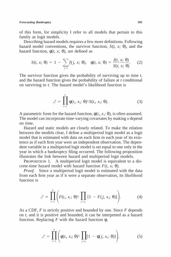
Describing hazard models requires a few more definitions. Followinghazard model conventions, the survivor function, S(t, x; θ), and thehazard function, φ(t, x; θ), are defined as

S(t, x; θ) 5 1 2j,t

f( j, x; θ), φ(t, x; θ) 5f(t, x; θ)S(t, x; θ)

. (2)

The survivor function gives the probability of surviving up to time t,and the hazard function gives the probability of failure at t conditionalon surviving to t. The hazard model’s likelihood function is

L 5 pn

i51

φ(ti, xi; θ)yi S(ti, xi; θ). (3)

A parametric form for the hazard function, φ(ti, xi; θ), is often assumed.The model can incorporate time-varying covariates by making x dependon time.

Hazard and static models are closely related. To make the relationbetween the models clear, I define a multiperiod logit model as a logitmodel that is estimated with data on each firm in each year of its exis-tence as if each firm year were an independent observation. The depen-dent variable in a multiperiod logit model is set equal to one only in theyear in which a bankruptcy filing occurred. The following propositionillustrates the link between hazard and multiperiod logit models.

Proposition 1. A multiperiod logit model is equivalent to a dis-crete-time hazard model with hazard function F(t, x; θ).

Proof. Since a multiperiod logit model is estimated with the datafrom each firm year as if it were a separate observation, its likelihoodfunction is

L 5 pn

i511F(ti, xi; θ)yi p

j, ti

[1 2 F( j, xi; θ)]2. (4)

As a CDF, F is strictly positive and bounded by one. Since F dependson t, and it is positive and bounded, it can be interpreted as a hazardfunction. Replacing F with the hazard function φ,

L 5 pn

i511φ(ti, xi; θ)yi p

j,t i

[1 2 φ( j, xi; θ)]2. (5)


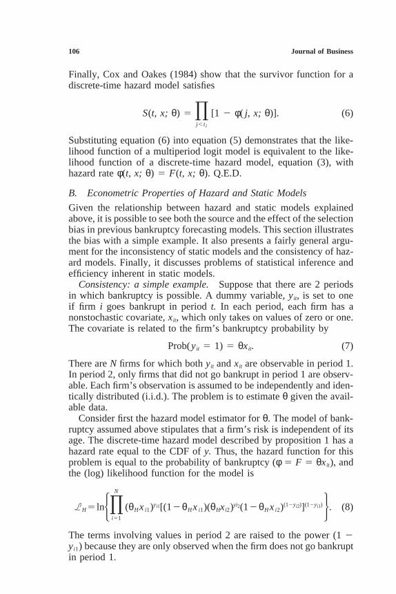
Finally, Cox and Oakes (1984) show that the survivor function for adiscrete-time hazard model satisfies

S(t, x; θ) 5 pj, t i

[1 2 φ( j, x; θ)]. (6)

Substituting equation (6) into equation (5) demonstrates that the like-lihood function of a multiperiod logit model is equivalent to the like-lihood function of a discrete-time hazard model, equation (3), withhazard rate φ(t, x; θ) 5 F(t, x; θ). Q.E.D.

B. Econometric Properties of Hazard and Static Models

Given the relationship between hazard and static models explainedabove, it is possible to see both the source and the effect of the selectionbias in previous bankruptcy forecasting models. This section illustratesthe bias with a simple example. It also presents a fairly general argu-ment for the inconsistency of static models and the consistency of haz-ard models. Finally, it discusses problems of statistical inference andefficiency inherent in static models.

Consistency: a simple example. Suppose that there are 2 periodsin which bankruptcy is possible. A dummy variable, yit, is set to oneif firm i goes bankrupt in period t. In each period, each firm has anonstochastic covariate, xit, which only takes on values of zero or one.The covariate is related to the firm’s bankruptcy probability by

Prob(yit 5 1) 5 θxit. (7)

There are N firms for which both yit and xit are observable in period 1.In period 2, only firms that did not go bankrupt in period 1 are observ-able. Each firm’s observation is assumed to be independently and iden-tically distributed (i.i.d.). The problem is to estimate θ given the avail-able data.

Consider first the hazard model estimator for θ. The model of bank-ruptcy assumed above stipulates that a firm’s risk is independent of itsage. The discrete-time hazard model described by proposition 1 has ahazard rate equal to the CDF of y. Thus, the hazard function for thisproblem is equal to the probability of bankruptcy (φ 5 F 5 θxit), andthe (log) likelihood function for the model is

LH 5 ln5pN

i51

(θHx i1)yi1[(12θHx i1)(θHxi2)yi2(12θH x i2)(12yi2)](12yi1)6. (8)

The terms involving values in period 2 are raised to the power (1 2yi1) because they are only observed when the firm does not go bankruptin period 1.


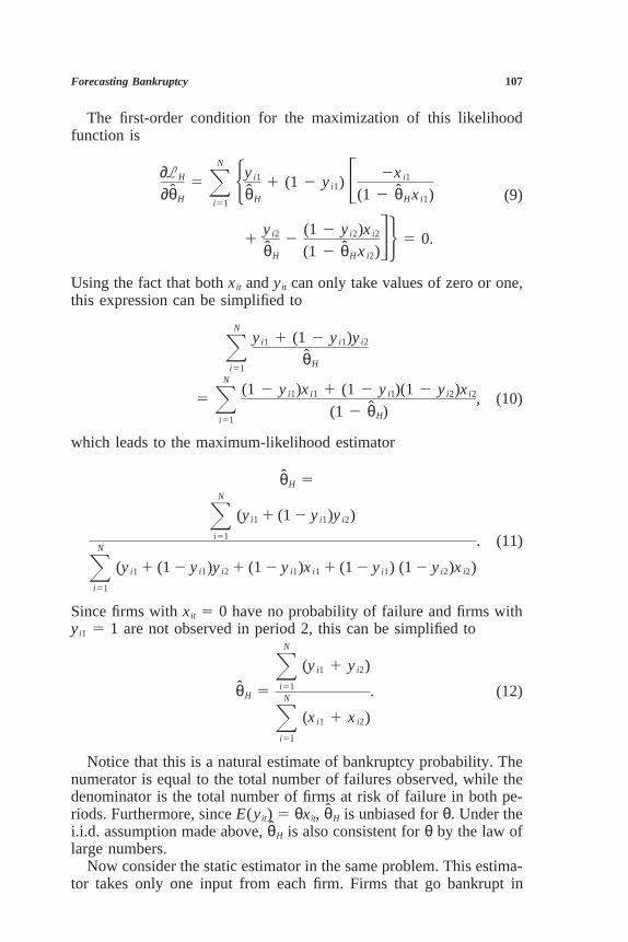
The first-order condition for the maximization of this likelihoodfunction is

∂LH

∂θH

5 ^N

i515y i1

θH

1 (1 2 y i1) 3 2x i1

(1 2 θHx i1) (9)

1y i2

θH

2(1 2 y i2)x i2

(1 2 θHx i2)46 5 0.

Using the fact that both xit and yit can only take values of zero or one,this expression can be simplified to

^N

i51

y i1 1 (1 2 y i1)y i2

θH

5 ^N

i51

(1 2 y i1)x i1 1 (1 2 y i1)(1 2 y i2)x i2

(1 2 θH), (10)

which leads to the maximum-likelihood estimator

θH 5

^N

i51

(y i1 1 (1 2 y i1)y i2)

^N

i51

(y i1 1 (1 2 y i1)y i2 1 (1 2 y i1)x i1 1 (1 2 y i1) (1 2 y i2)x i2)

. (11)

Since firms with xit 5 0 have no probability of failure and firms withyi1 5 1 are not observed in period 2, this can be simplified to

θH 5^

N

i51

(y i1 1 y i2)

^N

i51

(x i1 1 x i2)

. (12)

Notice that this is a natural estimate of bankruptcy probability. Thenumerator is equal to the total number of failures observed, while thedenominator is the total number of firms at risk of failure in both pe-riods. Furthermore, since E(yit) 5 θxit, θH is unbiased for θ. Under thei.i.d. assumption made above, θH is also consistent for θ by the law oflarge numbers.

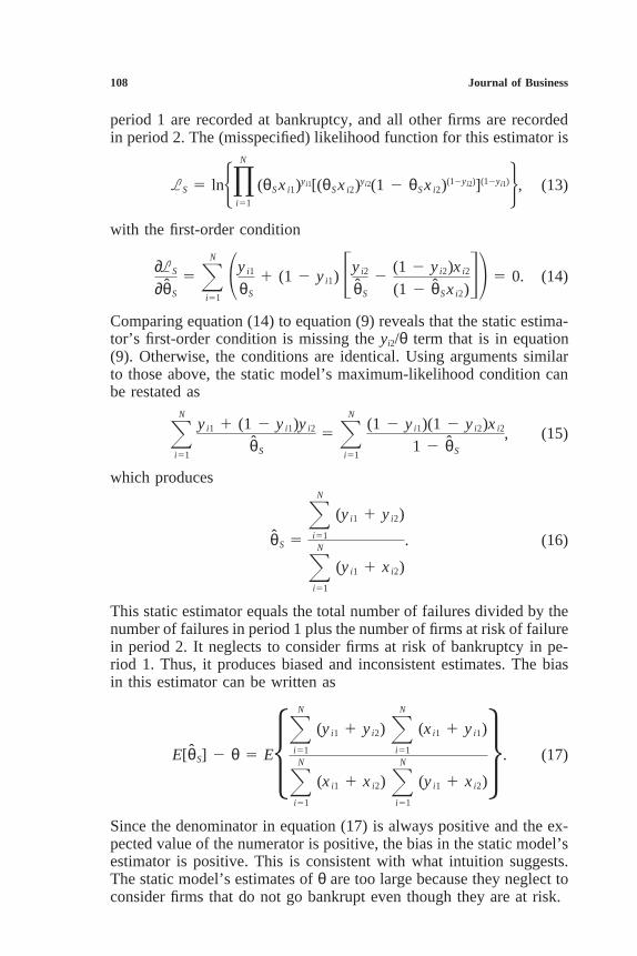
Now consider the static estimator in the same problem. This estima-tor takes only one input from each firm. Firms that go bankrupt in


period 1 are recorded at bankruptcy, and all other firms are recordedin period 2. The (misspecified) likelihood function for this estimator is

LS 5 ln5pN

i51

(θS x i1)yi1[(θS x i2)yi2(1 2 θS x i2)(12yi2)](12yi1)6, (13)

with the first-order condition

∂LS

∂θS

5 ^N

i511y i1

θS

1 (1 2 y i1) 3y i2

θS

2(1 2 y i2)x i2

(1 2 θS x i2)42 5 0. (14)

Comparing equation (14) to equation (9) reveals that the static estima-tor’s first-order condition is missing the yi2/θ term that is in equation(9). Otherwise, the conditions are identical. Using arguments similarto those above, the static model’s maximum-likelihood condition canbe restated as

^N

i51

y i1 1 (1 2 y i1)y i2

θS

5 ^N

i51

(1 2 y i1)(1 2 y i2)x i2

1 2 θS

, (15)

which produces

θS 5^

N

i51

(y i1 1 y i2)

^N

i51

(y i1 1 x i2)

. (16)

This static estimator equals the total number of failures divided by thenumber of failures in period 1 plus the number of firms at risk of failurein period 2. It neglects to consider firms at risk of bankruptcy in pe-riod 1. Thus, it produces biased and inconsistent estimates. The biasin this estimator can be written as

E[θS] 2 θ 5 E5^N

i51

(y i1 1 y i2) ^N

i51

(x i1 1 y i1)

^N

i51

(x i1 1 x i2) ^N

i51

(y i1 1 x i2)6. (17)

Since the denominator in equation (17) is always positive and the ex-pected value of the numerator is positive, the bias in the static model’sestimator is positive. This is consistent with what intuition suggests.The static model’s estimates of θ are too large because they neglect toconsider firms that do not go bankrupt even though they are at risk.


This simple example ignores many common complications. It as-sumes a simple structure and just two periods. In the next subsection,the consistency of more general static estimators is explored.

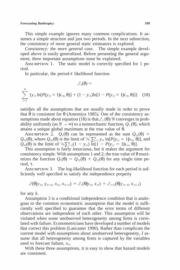
Consistency: the more general case. The simple example devel-oped above is easily generalized. Before presenting the general argu-ment, three important assumptions must be explained.

Assumption 1. The static model is correctly specified for 1 pe-riod.

In particular, the period-τ likelihood function

Lτ(θ) 5

^N

i51

{y iτ ln[P(y iτ 5 1|x iτ, θ)] 1 (1 2 y iτ)ln[1 2 P(y iτ 5 1|x iτ, θ)]} (18)

satisfies all the assumptions that are usually made in order to provethat θ is consistent for θ (Amemiya 1985). One of the consistency as-sumptions made about equation (18) is that Lτ (θ)/N converges in prob-ability uniformly (as N → ∞) to a nonstochastic function, Qτ (θ), whichattains a unique global maximum at the true value of θ.

Assumption 2. Qτ(θ) can be represented as the sum Qτ1(θ) 1Qτ2(θ), where Qτ1(θ) is the limit of 1/N ∑N

i51 yiτ ln[P(yiτ 5 1|xiτ, θ)], andQτ2(θ) is the limit of 1/N∑N

i51(1 2 yiτ) ln[1 2 P(yiτ 5 1|xiτ, θ)].This assumption is fairly innocuous, but it makes the argument for

consistency simple. With assumptions 1 and 2, the true value of θ maxi-mizes the function Qτ(θ) 5 Qτ1(θ) 1 Qτ2(θ) for any single time pe-riod, τ.

Assumption 3. The log-likelihood function for each period is suf-ficiently well specified to satisfy the independence property

L(θ|y iτ, yiτ1k, xiτ, xiτ1k) 5 Lτ(θ|y iτ, x iτ) 1 Lτ1k(θ|y iτ1k, x iτ1k)

for any k.Assumption 3 is a conditional independence condition that is analo-

gous to the common econometric assumption that the model is suffi-ciently well specified to guarantee that the error terms of differentobservations are independent of each other. This assumption will beviolated when some unobserved heterogeneity among firms is corre-lated with failure. Econometricians have developed a number of modelsthat correct this problem (Lancaster 1990). Rather than complicate thecurrent model with assumptions about unobserved heterogeneity, I as-sume that all heterogeneity among firms is captured by the variablesused to forecast failure, xit.

With these three assumptions, it is easy to show that hazard modelsare consistent.


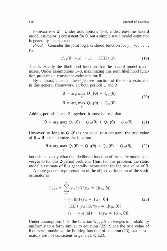
Proposition 2. Under assumptions 1–3, a discrete-time hazardmodel estimator is consistent for θ, but a simple static model estimatoris generally inconsistent.

Proof. Consider the joint log likelihood function for yi1, yi2, . . . ,yiT,

L1,T(θ) 5 L1 1 L2 1 ⋅ ⋅ ⋅ 1 LT. (19)

This is exactly the likelihood function that the hazard model maxi-mizes. Under assumptions 1–3, maximizing this joint likelihood func-tion produces a consistent estimator for θ.

By contrast, consider the objective function of the static estimatorin this general framework. In both periods 1 and 2

θ 5 arg maxθ

Q 11(θ) 1 Q 12(θ)(20)

θ 5 arg maxθ

Q 21(θ) 1 Q 22(θ).

Adding periods 1 and 2 together, it must be true that

θ 5 arg maxθ

Q 11(θ) 1 Q 12(θ) 1 Q 21(θ) 1 Q 22(θ). (21)

However, as long as Q12(θ) is not equal to a constant, the true valueof θ will not maximize the function

θ ≠ arg maxθ

Q S(θ) 5 Q 11(θ) 1 Q 21(θ) 1 Q 22(θ), (22)

but this is exactly what the likelihood function of the static model con-verges to for this 2-period problem. Thus, for this problem, the staticmodel’s estimate of θ is generally inconsistent for the true value of θ.

A more general representation of the objective function of the staticestimator is

GS;1,T 5 ^N

i51

y i1 ln[P(y i1 5 1|x i1, θ)]

1 y i2 ln[P(y i2 5 1|x i2, θ)] (23)

1 ⋅ ⋅ ⋅ 1 y iT ln[P(y iT 5 1|x iT, θ)]

1 (1 2 y iT) ln[1 2 P(y iT 5 1|x iT, θ)].

Under assumptions 1–3, the function GS;1,T/N converges in probabilityuniformly to a form similar to equation (22). Since the true value ofθ does not maximize the limiting function of equation (23), static esti-mators are not consistent in general. Q.E.D.


C. Inference and Efficiency

Since the parameter estimates produced by static models are biasedand inconsistent, tests of statistical significance performed with staticmodels are invalid. Thus, it is not clear that the variables associatedwith bankruptcy by static models are significant predictors. This issueis explored in detail in the empirical work below.

The connection between the hazard and logit models implies thateven if static models were consistent, hazard models should be moreaccurate. While each firm has a time series of annual observations,static models are estimated only with each firm’s last observation. Haz-ard models take advantage of much more data. They are equivalent tologit models in which no firm-year data points have been excluded.Unlike static models, hazard models exploit all of the data available.Thus, for both consistency and efficiency, hazard models are preferableto static models.

III. Estimating the Hazard Function

The previous section shows that hazard models are superior to staticmodels for forecasting bankruptcy. In practice, however, many hazardmodels are difficult to estimate because of their nonlinear likelihoodfunctions and time-varying covariates. Proposition 1 implies that it ispossible to estimate discrete-time hazard models with a computer pro-gram that estimates logit models. To estimate a hazard model with alogit program, each year in which the firm survives is included in thelogit program’s ‘‘sample’’ as a firm that did not fail. Each bankruptfirm contributes only one failure observation (yit 5 1) to the logitmodel. Time-varying covariates are incorporated simply by using eachfirm’s annual data for its firm-year logit observations. Estimating haz-ard models with a logit program is so simple and intuitive that it hasbeen done by academics and regulators without a hazard model justifi-cation.2

Making statistical inferences in a hazard model estimated with a logitprogram is simple. Since the logit and hazard models have the samelikelihood function, they have the same asymptotic variance-covariancematrix (Amemiya 1985). However, the test statistics produced by alogit program are incorrect for the hazard model because they assumethat the number of independent observations used to estimate the modelis the number of firm years in the data. Calculating correct test statisticsrequires adjusting the sample size assumed by the logit program to

2. Pagano, Panetta, and Zingales (1998) and Denis, Denis, and Sarin (1997) use modelslike the hazard model described here to forecast initial public offerings and executive turn-over. The Pension Benefits Guarantee Corporation forecasts bankruptcies by estimating alogit model by firm year.


account for the lack of independence between firm-year observations.The firm-year observations of a particular firm cannot be independent,since a firm cannot fail in period t if it failed in period t 2 1. Likewise,a firm that survives to period t cannot have failed in period t 2 1. Forthe hazard model, each firm’s entire life span is one observation. Thus,the correct value of n for test statistics is the number of firms in thedata, not the number of firm years. The χ2 test statistics produced bylogit programs are of the form

1n

(µk 2 µ0)′S21(µk 2 µ0) , χ2(k), (24)

where there are k estimated moments being tested against k null hypoth-eses, µ0. Dividing these test statistics by the average number of firmyears per firm makes the logit program’s statistics correct for the hazardmodel. Unreported estimates of a proportional hazard model confirmthat standard hazard models produce coefficient estimates and test sta-tistics that are similar to those produced by the discrete-time hazardmodel described here.

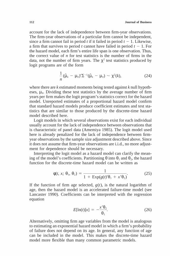
Logit models in which several observations exist for each individualusually account for the lack of independence between observations thatis characteristic of panel data (Amemiya 1985). The logit model usedhere is already penalized for the lack of independence between firm-year observations by the sample size adjustment described above. Sinceit does not assume that firm-year observations are i.i.d., no more adjust-ment for dependence should be necessary.

Interpreting the logit model as a hazard model can clarify the mean-ing of the model’s coefficients. Partitioning θ into θ1 and θ2, the hazardfunction for the discrete-time hazard model can be written as

φ(t, x; θ1, θ2) 51

1 1 Exp(g(t)′θ1 1 x ′θ2). (25)

If the function of firm age selected, g(t), is the natural logarithm ofage, then the hazard model is an accelerated failure-time model (seeLancaster 1990). Coefficients can be interpreted with the regressionequation

E[ln(t)|x] 5 2x ′θ2

θ1

. (26)

Alternatively, omitting firm age variables from the model is analogousto estimating an exponential hazard model in which a firm’s probabilityof failure does not depend on its age. In general, any function of agecan be included in the model. This makes the discrete-time hazardmodel more flexible than many common parametric models.


IV. The Data

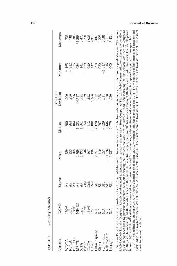
To compare hazard to static model forecasts, I estimate both hazardand static models and examine their out-of-sample accuracy. Only firmsin the intersection of the Compustat Industrial File and the CRSP DailyStock Return File for New York Stock Exchange (NYSE) and Ameri-can Stock Exchange (AMEX) stocks are included in the sample. Firmsthat began trading before 1962 or after 1992 are excluded. Firms withCRSP Standard Industrial Classification (SIC) codes from 6,000 to6,999 (financial firms) are also excluded. Table 1 provides summarystatistics for all of the independent variables described below.

A. Bankruptcy Data

I collected bankruptcy data from the Wall Street Journal Index, theCapital Changes Reporter, and the Compustat Research File. I alsosearched for firms whose stock was delisted from the NYSE or AMEXin the Directory of Obsolete Securities (Financial Stock Guide Service[1993]) and Nexis. All firms that filed for any type of bankruptcy within5 years of delisting are considered bankrupt. The final sample contains300 bankruptcies between 1962 and 1992.

The variable of interest in the hazard model is firm age. In this article,a firm’s age is defined as the number of calendar years it has beentraded on the NYSE or AMEX. So, for example, if a firm began tradingon the NYSE in 1964 and then merged in 1965, it would contributetwo firm-year observations to the logit model. One observation wouldgive the firm’s age as 1 year and the other would indicate that the firm’sage was 2 years. The dependent variable associated with both of theseobservations would be equal to zero, indicating no bankruptcy oc-curred. If the firm filed for bankruptcy, only its second firm-year obser-vation would have a dependent variable value of one.

I use the firm’s trading age as the variable to be explained becausethere is no attractive alternative to measure how long the firm has beena viable enterprise. Since a firm must meet a number of requirementsto be listed by an exchange, firms are fairly homogeneous when initiallylisted. However, a firm can be incorporated as a small speculative con-cern or as a large holding company, making the firm’s age since incor-poration less economically meaningful than its age since listing. In thehazard models I estimate, firm age is never statistically significant aftercontrolling for other firm characteristics.

B. Independent Variables

I estimate models with several different sets of independent variables.The forecasting models incorporate Altman’s (1968) and Zmijewski’s(1984) independent variables, as well as some new market-driven inde-pendent variables described in this section.


TA

BL

E1

Sum

mar

ySt

atis

tics

Stan

dard

Var

iabl

eC

OM

PSo

urce

Mea

nM

edia

nD

evia

tion

Min

imum

Max

imum

WC

/TA

179/

6A

lt.2

89.3

00.2

002

.165

.736

RE

/TA

36/6

Alt

.255

.264

.256

2.9

12.7

81E

BIT

/TA

178/

6A

lt.1

05.1

04.0

962

.225

.386

ME

/TL

ME

/181

Alt

2.79

91.

223

4.71

7.0

3431

.893

S/T

A12

/6A

lt1.

493

1.36

1.9

21.1

415.

475

NI/

TA

172/

6Z

mi

.048

.054

.079

2.3

29.2

31T

L/T

A18

1/6

Zm

i.5

07.5

12.1

92.0

901.

028

CA

/CL

4/5

Zm

i2.

439

2.10

81.

460

.447

9.21

4D

efau

ltsp

read

N.A

.Sh

u2.

251

2.17

0.8

27.5

903.

860

Sigm

aN

.A.

Shu

.110

.097

.055

.030

.325

r it2

12

r mt2

1N

.A.

Shu

.057

2.0

29.5

112

0.81

72.

181

Rel

ativ

esi

zeN

.A.

Shu

210

.076

210

.146

1.63

82

13.6

162

6.11

5L

n(a

ge)

N.A

.Sh

u1.

937

2.07

9.9

20.0

003.

434

Not

e.—

Tab

le1

repo

rts

sum

mar

yst

atis

tics

for

all

ofth

eva

riab

les

used

tofo

reca

stba

nkru

ptcy

.Eac

hob

serv

atio

nre

pres

ents

apa

rtic

ular

firm

ina

part

icul

arye

ar.T

heco

lum

nla

bele

dC

OM

Plis

tsth

eC

ompu

stat

vari

able

num

bers

used

toco

nstr

uct

the

vari

able

sth

atar

eta

ken

from

Com

pust

at.

The

col.

labe

led

Sour

cein

dica

tes

whe

ther

the

vari

able

inqu

estio

nha

sbe

enus

edby

prev

ious

rese

arch

ers,

with

Alt

indi

catin

gth

atth

eva

riab

lew

asus

edby

Altm

an(1

968)

,Z

mi

indi

catin

gth

atth

eva

riab

lew

asus

edby

Zm

ijew

ski

(198

4),a

ndSh

uin

dica

ting

that

the

vari

able

isne

wto

this

artic

le.I

nth

een

tire

sam

ple,

ther

ear

e30

0ba

nkru

ptci

esam

ong

3,18

2fir

ms

and

39,7

45fir

mye

ars.

The

sam

ple

peri

odis

from

1962

to19

92.

All

vari

able

sar

etr

unca

ted

atth

eni

nety

-nin

than

dfir

stpe

rcen

tiles

,so

the

min

imum

and

max

imum

quan

titie

sre

port

edar

eac

tual

lyth

ose

quan

tiles

.N

.A.5

not

appl

icab

le.R

atio

s:W

C/T

A5

wor

king

capi

tal

toto

tal

asse

ts;

RE

/TA

5re

tain

edea

rnin

gsto

tota

las

sets

;E

BIT

/TA

5ea

rnin

gsbe

fore

inte

rest

and

taxe

sto

tota

las

sets

;M

E/T

L5

mar

ket

equi

tyto

tota

llia

bilit

ies;

S/T

A5

sale

sto

tota

las

sets

;NI/

TA

5ne

tinc

ome

toto

tala

sset

s;T

L/T

A5

tota

llia

bilit

ies

toto

tal

asse

ts;C

A/C

L5

curr

ent

asse

tsto

curr

ent

liabi

litie

s.


Altman’s variables are described extensively in Altman (1993). Theyinclude the ratios of working capital to total assets (WC/TA), retainedearnings to total assets (RE/TA), earnings before interest and taxes tototal assets (EBIT/TA), market equity to total liabilities (ME/TL), andsales to total assets (S/TA). The Compustat item numbers that I usedto construct Altman’s variables appear with the variables’ summarystatistics in table 1.

In order to make my forecasting exercise realistic, I lag all data toensure that the data are observable in the beginning of the year in whichbankruptcy is observed. To construct Altman’s (and Zmijewski’s) vari-ables, I lag Compustat data to ensure that each firm’s fiscal year endsat least 6 months before the beginning of the year of interest. I lag themarket-driven variables described below in a similar fashion.

There are a number of extreme values among the observations ofAltman’s ratios constructed from raw Compustat data. To ensure thatstatistical results are not heavily influenced by outliers, I set all observa-tions higher than the ninety-ninth percentile of each variable to thatvalue. All values lower than the first percentile of each variable aretruncated in the same manner. Zmijewski’s variables and the market-driven variables I introduce below are also truncated to avoid outliers.Unreported results with untruncated data are generally similar to theresults I report. The minimum and maximum numbers reported in table1 are calculated after truncation.

Zmijewski’s variables include the ratio of net income to total assets(NI/TA), the ratio of total liabilities to total assets (TL/TA), and theratio of current assets to current liabilities (CA/CL). As with Altman’svariables, the Compustat item numbers used to construct each of thesevariables appears in table 1. The data are lagged and truncated as de-scribed above.

Because the market equity of firms that are close to bankruptcy istypically discounted by traders, firm size is a very important bankruptcypredicting variable. Each firm’s market capitalization is measured atthe end of the year before the observation year. To make size stationary,the logarithm of each firm’s size relative to the total size of the NYSEand AMEX market is used. These data are all readily available in theCRSP database. The average of relative size is negative because it isthe logarithm of a generally small fraction.

If traders discount the equity of firms that are close to bankruptcy,then a firm’s past excess returns should predict bankruptcy as well asits market capitalization. I measure each firm’s past excess return inyear t as the return of the firm in year t 2 1 minus the value-weightedCRSP NYSE/AMEX index return in year t 2 1. Each firm’s annualreturns are calculated by cumulating monthly returns. When some ofa firm’s monthly returns are missing, the value-weighted CRSP NYSE/AMEX index return is substituted for the missing returns. The average


excess return reported in table 1 is a small positive number becauseequal-weighted returns are typically higher than value-weighted re-turns.

The last market-driven variable that I use is the idiosyncratic stan-dard deviation of each firm’s stock returns, denoted sigma in the tablesbelow. Sigma is strongly related to bankruptcy both statistically andlogically. If a firm has more variable cash flows (and hence more vari-able stock returns), then the firm ought to have a higher probability ofbankruptcy. Sigma may also measure something like operating lever-age. I calculate each firm’s sigma for year t by regressing each stock’smonthly returns in year t 2 1 on the value-weighted NYSE/AMEXindex return for the same year. Sigma is the standard deviation of theresidual of this regression. I drop values calculated with regressionsbased on less than 12 months of returns. To avoid outliers, relativesize, past returns, and sigma are all truncated at the ninety-ninth andfirst percentile values in the same manner as all other independent vari-ables.

Since a complete set of explanatory variables is not always observ-able for each firm year, I substitute variable values from past years formissing values in some cases. This does not present an econometricproblem because, for example, accounting ratios observed in year t arestill observable in years t 1 1 and t 1 2. By filling in missing data,the number of firm years available to estimate Altman’s model risesfrom 27,665 to 28,226. The number of bankruptcies available to iden-tify rises from 201 to 229.

V. Forecasting Results

In this section, I report parameter estimates for various forecastingmodels, and I compare the out-of-sample accuracy of all the modelsconsidered. Unreported estimates of analogous proportional hazardmodels are approximately proportional to the estimates reported.

A. Models with Altman’s Variables

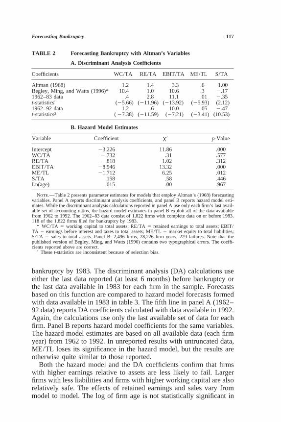
Table 2 reports the results of estimating models with Altman’s vari-ables. Panel A displays Altman’s original discriminant function, a newset of coefficients calculated by Begley, Ming, and Watts (1996) andtwo functions calculated with my bankruptcy data.3 The coefficients inthe third line of the table (1962–83 data) are calculated only with dataavailable in 1983. Those data consist of 1,822 firms that have completedata for at least 1 year between 1962 and 1983, 118 of which filed for

3. Altman (1993) discusses the interpretation of discriminant analysis coefficients exten-sively. The published version of Begley, Ming, and Watts (1996) contains two typographi-cal errors. The coefficients reported in table 2 are correct.


TABLE 2 Forecasting Bankruptcy with Altman’s Variables

A. Discriminant Analysis Coefficients

Coefficients WC/TA RE/TA EBIT/TA ME/TL S/TA

Altman (1968) 1.2 1.4 3.3 .6 1.00Begley, Ming, and Watts (1996)* 10.4 1.0 10.6 .3 2.171962–83 data .4 2.8 11.1 .01 2.35t-statistics† (25.66) (211.96) (213.92) (25.93) (2.12)1962–92 data 1.2 .6 10.0 .05 2.47t-statistics† (27.38) (211.59) (27.21) (23.41) (10.53)

B. Hazard Model Estimates

Variable Coefficient χ2 p-Value

Intercept 23.226 11.86 .000WC/TA 2.732 .31 .577RE/TA 2.818 1.02 .312EBIT/TA 28.946 13.32 .000ME/TL 21.712 6.25 .012S/TA .158 .58 .446Ln(age) .015 .00 .967

Note.—Table 2 presents parameter estimates for models that employ Altman’s (1968) forecastingvariables. Panel A reports discriminant analysis coefficients, and panel B reports hazard model esti-mates. While the discriminant analysis calculations reported in panel A use only each firm’s last avail-able set of accounting ratios, the hazard model estimates in panel B exploit all of the data availablefrom 1962 to 1992. The 1962–83 data consist of 1,822 firms with complete data on or before 1983.118 of the 1,822 firms filed for bankruptcy by 1983.

* WC/TA 5 working capital to total assets; RE/TA 5 retained earnings to total assets; EBIT/TA 5 earnings before interest and taxes to total assets; ME/TL 5 market equity to total liabilities;S/TA 5 sales to total assets. Panel B: 2,496 firms, 28,226 firm years, 229 failures. Note that thepublished version of Begley, Ming, and Watts (1996) contains two typographical errors. The coeffi-cients reported above are correct.

† These t-statistics are inconsistent because of selection bias.

bankruptcy by 1983. The discriminant analysis (DA) calculations useeither the last data reported (at least 6 months) before bankruptcy orthe last data available in 1983 for each firm in the sample. Forecastsbased on this function are compared to hazard model forecasts formedwith data available in 1983 in table 3. The fifth line in panel A (1962–92 data) reports DA coefficients calculated with data available in 1992.Again, the calculations use only the last available set of data for eachfirm. Panel B reports hazard model coefficients for the same variables.The hazard model estimates are based on all available data (each firmyear) from 1962 to 1992. In unreported results with untruncated data,ME/TL loses its significance in the hazard model, but the results areotherwise quite similar to those reported.

Both the hazard model and the DA coefficients confirm that firmswith higher earnings relative to assets are less likely to fail. Largerfirms with less liabilities and firms with higher working capital are alsorelatively safe. The effects of retained earnings and sales vary frommodel to model. The log of firm age is not statistically significant in


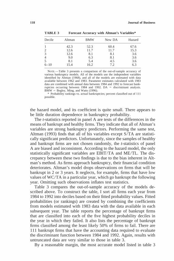
TABLE 3 Forecast Accuracy with Altman’s Variables*

Decile Altman BMW New DA Hazard

1 42.3 52.3 60.4 67.62 12.6 11.7 11.7 15.33 12.6 8.1 8.1 3.64 9.0 6.3 8.1 3.65 8.1 5.4 4.5 3.66–10 15.4 16.2 7.2 6.3

Note.—Table 3 presents a comparison of the out-of-sample accuracy ofvarious bankruptcy models. All of the models use the independent variablesidentified by Altman (1968), and all of the models are estimated with dataavailable between 1962 and 1983. Parameter estimates calculated with 1983data are combined with annual data between 1984 and 1992 to forecast bank-ruptcies occurring between 1984 and 1992. DA 5 discriminant analysis.BMW 5 Begley, Ming, and Watts (1996).

* Probability rankings vs. actual bankruptcies; percent classified out of 111possible.

the hazard model, and its coefficient is quite small. There appears tobe little duration dependence in bankruptcy probability.

The t-statistics reported in panel A are tests of the differences in themeans of bankrupt and healthy firms. They indicate that all of Altman’svariables are strong bankruptcy predictors. Performing the same test,Altman (1993) finds that all of his variables except S/TA are statisti-cally significant predictors. Unfortunately, since the samples of healthyand bankrupt firms are not chosen randomly, the t-statistics of panelA are biased and inconsistent. According to the hazard model, the onlystatistically significant variables are EBIT/TA and ME/TL. The dis-crepancy between these two findings is due to the bias inherent in Alt-man’s method. As firms approach bankruptcy, their financial conditiondeteriorates. Altman’s model drops observations on firms that will bebankrupt in 2 or 3 years. It neglects, for example, firms that have lowvalues of WC/TA in a particular year, which go bankrupt the followingyear. Omitting such observations inflates test statistics.

Table 3 compares the out-of-sample accuracy of the models de-scribed above. To construct the table, I sort all firms each year from1984 to 1992 into deciles based on their fitted probability values. Fittedprobabilities (or rankings) are created by combining the coefficientsfrom models estimated with 1983 data with the data available in eachsubsequent year. The table reports the percentage of bankrupt firmsthat are classified into each of the five highest probability deciles inthe year in which they failed. It also lists the percentage of bankruptfirms classified among the least likely 50% of firms to fail. There are111 bankrupt firms that have the accounting data required to evaluatethe discriminant function between 1984 and 1992. Again, results withuntruncated data are very similar to those in table 3.

By a reasonable margin, the most accurate model listed in table 3


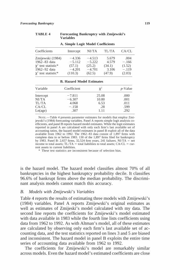
TABLE 4 Forecasting Bankruptcy with Zmijewski’sVariables

A. Simple Logit Model Coefficients

Coefficients Intercept NI/TA TL/TA CA/CL

Zmijewski (1984) 24.336 24.513 5.679 .0041962–83 data 25.112 25.222 4.579 2.166χ2 test statistic* (57.1) (25.2) (34.1) (1.52)1962–92 data 24.201 24.701 3.106 2.119χ2 test statistic* (110.3) (62.5) (47.9) (2.03)

B. Hazard Model Estimates


Intercept 27.811 25.08 .000NI/TA 26.307 10.80 .001TL/TA 4.068 6.53 .011CA/CL 2.158 .28 .599Ln(age) .307 1.11 .292

Note.—Table 4 presents parameter estimates for models that employ Zmi-jewski’s (1984) forecasting variables. Panel A reports simple logit analysis co-efficients, and panel B reports hazard model estimates. While the logit estimatesreported in panel A are calculated with only each firm’s last available set ofaccounting ratios, the hazard model estimates in panel B exploit all of the dataavailable from 1962 to 1992. The 1962–83 data consist of 1,897 firms withcomplete data in or before 1983. 130 of the 1,897 firms filed for bankruptcyby 1983. Panel B: 2,657 firms, 32,524 firm years, 241 failures. NI/TA 5 netincome to total assets; TL/TA 5 total liabilities to total assets; CA/CL 5 cur-rent assets to current liabilities.

* These test statistics are inconsistent because of selection bias.

is the hazard model. The hazard model classifies almost 70% of allbankruptcies in the highest bankruptcy probability decile. It classifies96.6% of bankrupt firms above the median probability. The discrimi-nant analysis models cannot match this accuracy.

B. Models with Zmijewski’s Variables

Table 4 reports the results of estimating three models with Zmijewski’s(1984) variables. Panel A reports Zmijewski’s original estimates aswell as estimates of Zmijeski’s model calculated with my data. Thesecond line reports the coefficients for Zmijewski’s model estimatedwith data available in 1983 while the fourth line lists coefficients usingdata from 1962 to 1992. As with Altman’s model, all of these estimatesare calculated by observing only each firm’s last available set of ac-counting data, and the test statistics reported on lines 3 and 5 are biasedand inconsistent. The hazard model in panel B exploits the entire timeseries of accounting data available from 1962 to 1992.

The coefficients for Zmijewski’s model are remarkably similaracross models. Even the hazard model’s estimated coefficients are close


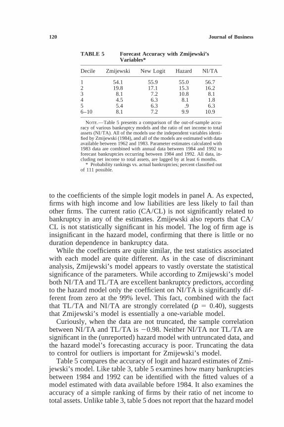
TABLE 5 Forecast Accuracy with Zmijewski’sVariables*

Decile Zmijewski New Logit Hazard NI/TA

1 54.1 55.9 55.0 56.72 19.8 17.1 15.3 16.23 8.1 7.2 10.8 8.14 4.5 6.3 8.1 1.85 5.4 6.3 .9 6.36–10 8.1 7.2 9.9 10.9

Note.—Table 5 presents a comparison of the out-of-sample accu-racy of various bankruptcy models and the ratio of net income to totalassets (NI/TA). All of the models use the independent variables identi-fied by Zmijewski (1984), and all of the models are estimated with dataavailable between 1962 and 1983. Parameter estimates calculated with1983 data are combined with annual data between 1984 and 1992 toforecast bankruptcies occurring between 1984 and 1992. All data, in-cluding net income to total assets, are lagged by at least 6 months.

* Probability rankings vs. actual bankruptcies; percent classified outof 111 possible.

to the coefficients of the simple logit models in panel A. As expected,firms with high income and low liabilities are less likely to fail thanother firms. The current ratio (CA/CL) is not significantly related tobankruptcy in any of the estimates. Zmijewski also reports that CA/CL is not statistically significant in his model. The log of firm age isinsignificant in the hazard model, confirming that there is little or noduration dependence in bankruptcy data.

While the coefficients are quite similar, the test statistics associatedwith each model are quite different. As in the case of discriminantanalysis, Zmijewski’s model appears to vastly overstate the statisticalsignificance of the parameters. While according to Zmijewski’s modelboth NI/TA and TL/TA are excellent bankruptcy predictors, accordingto the hazard model only the coefficient on NI/TA is significantly dif-ferent from zero at the 99% level. This fact, combined with the factthat TL/TA and NI/TA are strongly correlated (ρ 5 0.40), suggeststhat Zmijewski’s model is essentially a one-variable model.

Curiously, when the data are not truncated, the sample correlationbetween NI/TA and TL/TA is 20.98. Neither NI/TA nor TL/TA aresignificant in the (unreported) hazard model with untruncated data, andthe hazard model’s forecasting accuracy is poor. Truncating the datato control for outliers is important for Zmijewski’s model.

Table 5 compares the accuracy of logit and hazard estimates of Zmi-jewski’s model. Like table 3, table 5 examines how many bankruptciesbetween 1984 and 1992 can be identified with the fitted values of amodel estimated with data available before 1984. It also examines theaccuracy of a simple ranking of firms by their ratio of net income tototal assets. Unlike table 3, table 5 does not report that the hazard model


dominates alternative models. The hazard model does not even performbetter than the NI/TA sort. Each of the models appears fairly accurate,assigning between 54% and 56% of bankrupt firms to the highest bank-ruptcy probability decile. However, none of the three models appearsto add much explanatory power to NI/TA. This is not surprising, giventhat each of these models only includes one strong bankruptcy pre-dictor. Thus, while it is a little disappointing that the hazard modeldoes not outperform the logit model, it is not possible for one (mono-tonic) model to outperform another model if both are based on onlyone important bankruptcy predictor.

None of the forecasts made with Zmijewski’s model are as success-ful as the hazard model that uses Altman’s variables in table 3. Still,the variables in these two models measure similar things. Both EBIT/TA and NI/TA measure the profitability of the firm, while both ME/TLand TL/TA measure the firm’s leverage. A critical difference betweenAltman’s and Zmijewski’s variables is that Altman’s ME/TL containsa value determined in equilibrium by market traders rather than byaccounting conventions. In an effort to build bankruptcy models withmore power, two models that incorporate other market-driven variablesare described in the next section.

C. Models with Market-Driven Variables

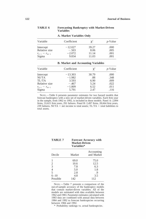
Parameter estimates for two hazard models that include market-drivenvariables appear in table 6. The model reported in panel A forecastsbankruptcies with market-driven variables exclusively while the modelin panel B combines market-driven variables with two accounting ra-tios from Zmijewski’s model. Because there is no evidence of durationdependence in bankruptcy probability, neither model contains the logof firm age as an explanatory variable. Both models are estimated withall data (each firm year) from 1962 to 1992. An important advantageof the model that is based solely on market-driven variables is thatfirms without Compustat data can remain in the model’s sample. Themodel in panel A is estimated with 33,621 firm years and 291 bankrupt-cies, while the model in panel B is estimated with only 28,664 firmyears and 239 bankruptcies. Estimates calculated with untruncated dataare quite similar to those reported.

All of the coefficients in both models have the expected signs.Larger, less volatile firms with high past returns are safer than small,volatile firms with low past returns. High net income and low liabilitiesare again associated with low risk. While all three of the market-drivenvariables are statistically significant in panel A, both NI/TA and sigmabecome insignificant when market variables and accounting ratios arecombined in panel B.

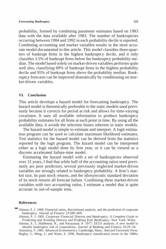
The accuracy of these models is examined in table 7. As in tables3 and 5, firms are sorted annually based on their implied bankruptcy


TABLE 6 Forecasting Bankruptcy with Market-DrivenVariables

A. Market Variables Only


Intercept 212.027 39.27 .000Relative size 2.503 8.06 .005rit21 2 rmt21 22.072 11.14 .001Sigma 9.834 11.03 .001

B. Market and Accounting Variables


Intercept 213.303 30.79 .000NI/TA 21.982 .88 .348TL/TA 3.593 6.90 .009Relative size 2.467 5.24 .022rit21 2 rmt21 21.809 6.52 .011Sigma 5.791 2.47 .116

Note.—Table 6 presents parameter estimates for two hazard models thatforecast bankruptcy with a new set of market-driven variables. Each firm yearin the sample, from 1962 to 1992, is included in these models. Panel A: 2,894firms, 33,621 firm years, 291 failures. Panel B: 2,497 firms, 28,664 firm years,239 failures. NI/TA 5 net income to total assets; TL/TA 5 total liabilities tototal assets.

TABLE 7 Forecast Accuracy withMarket-DrivenVariables*

AccountingDecile Market and Market

1 69.0 75.02 10.6 12.53 7.8 6.34 5.0 1.85 2.8 .96–10 4.8 3.5Possible 142 112

Note.—Table 7 presents a comparison of theout-of-sample accuracy of the bankruptcy modelsthat contain market-driven variables. All of themodels are estimated with data available between1962 and 1983. Parameter estimates calculated with1983 data are combined with annual data between1984 and 1992 to forecast bankruptcies occurringbetween 1984 and 1992.

* Probability rankings vs. actual bankruptcies.


probability, formed by combining parameter estimates based on 1983data with the data available after 1983. The number of bankruptciesoccurring between 1984 and 1992 in each probability decile is reported.Combining accounting and market variables results in the most accu-rate model documented in this article. This model classifies three-quar-ters of bankrupt firms in the highest bankruptcy decile, and it onlyclassifies 3.5% of bankrupt firms below the bankruptcy probability me-dian. The model based solely on market-driven variables performs quitewell also, classifying 69% of bankrupt firms in the highest probabilitydecile and 95% of bankrupt firms above the probability median. Bank-ruptcy forecasts can be improved dramatically by conditioning on mar-ket-driven variables.

VI. Conclusion

This article develops a hazard model for forecasting bankruptcy. Thehazard model is theoretically preferable to the static models used previ-ously because it corrects for period at risk and allows for time-varyingcovariates. It uses all available information to produce bankruptcyprobability estimates for all firms at each point in time. By using all theavailable data, it avoids the selection biases inherent in static models.

The hazard model is simple to estimate and interpret. A logit estima-tion program can be used to calculate maximum likelihood estimates.Test statistics for the hazard model can be derived from the statisticsreported by the logit program. The hazard model can be interpretedeither as a logit model done by firm year, or it can be viewed as adiscrete accelerated failure-time model.

Estimating the hazard model with a set of bankruptcies observedover 31 years, I find that while half of the accounting ratios used previ-ously are poor predictors, several previously neglected market-drivenvariables are strongly related to bankruptcy probability. A firm’s mar-ket size, its past stock returns, and the idiosyncratic standard deviationof its stock returns all forecast failure. Combining these market-drivenvariables with two accounting ratios, I estimate a model that is quiteaccurate in out-of-sample tests.

References

Altman, E. I. 1968. Financial ratios, discriminant analysis, and the prediction of corporatebankruptcy. Journal of Finance 23:589–609.

Altman, E. I. 1993. Corporate Financial Distress and Bankruptcy: A Complete Guide toPredicting and Avoiding Distress and Profiting from Bankruptcy. New York: Wiley.

Altman, E. I.; Haldeman, R.; and Narayanan, P. 1977. ZETA analysis: A new model toidentify bankruptcy risk of corporations. Journal of Banking and Finance 10:29–54.

Amemiya, T. 1985. Advanced Econometrics. Cambridge, Mass.: Harvard University Press.Begley, J.; Ming, J.; and Watts, S. 1996. Bankruptcy classification errors in the 1980s:


An empirical analysis of Altman’s and Ohlson’s models. Review of Accounting Studies1:267–84.

Cox, D. R., and Oakes, D. 1984. Analysis of Survival Data. New York: Chapman & Hall.Denis, D. J.; Denis, D. K.; and Sarin, A. 1997. Ownership structure and top executive

turnover. Journal of Financial Economics 45:193–221.Dichev, I. 1998. Is the risk of bankruptcy a systematic risk? Journal of Finance 53:1131–

48.Duffie, D., and Singleton, K. 1999. Modeling term structures of defaultable bonds. Review

of Financial Studies 12:687–720.Financial Stock Guide Service 1993. Directory of Obsolete Securities. Jersey City, N.J.:

Financial Information, Inc.Kiefer, N. M. 1988. Economic duration data and hazard functions. Journal of Economic

Literature 26:646–79.Lancaster, T. 1990. The Econometric Analysis of Transition Data. New York: Cambridge

University Press.Lau, A. H. L. 1987. A five-state financial distress prediction model. Journal of Accounting

Research 18:109–31.Ohlson, J. S. 1980. Financial ratios and the probabilistic prediction of bankruptcy. Journal

of Accounting Research 19:109–31.Pagano, M.; Panetta, F.; and Zingales, L. 1998. Why do companies go public? An empirical

analysis. Journal of Finance 53:27–64.Palepu, K. G. 1986. Predicting takeover targets: A methodological and empirical analysis.

Journal of Accounting and Economics 8:3–35.Queen, M., and Roll, R. 1987. Firm mortality: Using market indicators to predict survival.

Financial Analysts Journal (May–June): 9–26.Theodossiou, P. T. 1993. Predicting shifts in the mean of a multivariate time series process:

An application in predicting business failures. Journal of the American Statistical Associ-ation 88:441–49.

Zmijewski, M. E. 1984. Methodological issues related to the estimation of financial distressprediction models. Journal of Accounting Research 22:59–82.

shumway 2001

Documents

idiosyncratic

compustat

past stock

multiperiod

parameter

prefer hazard

unlike static

ta retained