series issn: 1938-1743 smsmsm ynthesis …gtsat/collection/morgan claypool... · synthesis lectures...
TRANSCRIPT
Mo
rg
an
& C
la
yp
oo
l
CM& Morgan Claypool Publishers&SYNTHESIS LECTURES ONMATHEMATICS AND STATISTICS
About SYNTHESIsThis volume is a printed version of a work that appears in the SynthesisDigital Library of Engineering and Computer Science. Synthesis Lecturesprovide concise, original presentations of important research and developmenttopics, published quickly, in digital and print formats. For more informationvisit www.morganclaypool.com
ISBN: 978-1-60845-658-1
9 781608 456581
90000
SYNTHESIS LECTURES ONMATHEMATICS AND STATISTICSMorgan Claypool Publishers&
w w w . m o r g a n c l a y p o o l . c o m
Series Editor: Steven G. Krantz, Washington University, St. Louis
Steven G. Krantz, Series Editor
Series ISSN: 1938-1743
MATRICES IN
ENG
INEERIN
G PRO
BLEMS
Matrices in Engineering ProblemsMarvin J. Tobias
This book is intended as an undergraduate text introducing matrix methods as they relate to engi-neeringproblems. It begins with the fundamentals of mathematics of matrices and determinants. Matrix inversionis discussed, with an introduction of the well known reduction methods. Equation sets are viewed asvector transformations, and the conditions of their solvability are explored.
Orthogonal matrices are introduced with examples showing application to many problems requiringthree dimensional thinking. The angular velocity matrix is shown to emerge from the differentiationof the 3-D orthogonal matrix, leading to the discussion of particle and rigid body dynamics.
The book continues with the eigenvalue problem and its application to multi-variable vibrations.Because the eigenvalue problem requires some operations with polynomials, a separate discussion ofthese is given in an appendix. The example of the vibrating string is given with a comparison of thematrix analysis to the continuous solution.
Matrices inEngineering Problems
Marvin J. Tobias
TOBIAS

Matrices in Engineering Problems
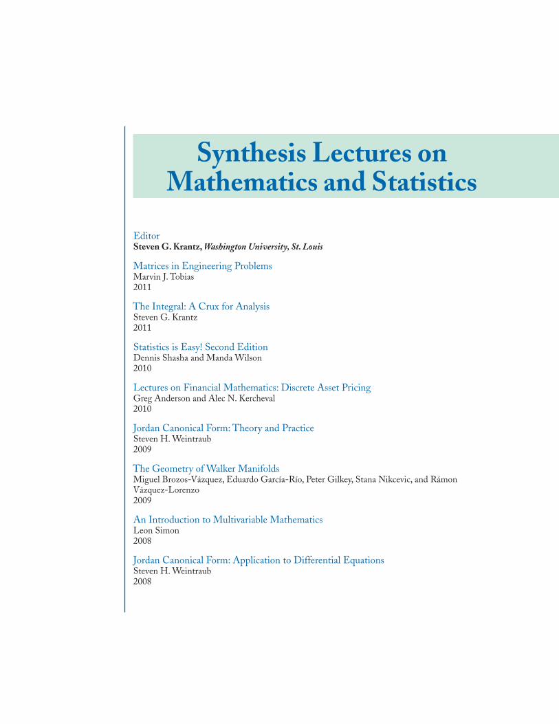
Synthesis Lectures onMathematics and Statistics
EditorSteven G. Krantz, Washington University, St. Louis
Matrices in Engineering ProblemsMarvin J. Tobias2011
The Integral: A Crux for AnalysisSteven G. Krantz2011
Statistics is Easy! Second EditionDennis Shasha and Manda Wilson2010
Lectures on Financial Mathematics: Discrete Asset PricingGreg Anderson and Alec N. Kercheval2010
Jordan Canonical Form: Theory and PracticeSteven H. Weintraub2009
The Geometry of Walker ManifoldsMiguel Brozos-Vázquez, Eduardo García-Río, Peter Gilkey, Stana Nikcevic, and RámonVázquez-Lorenzo2009
An Introduction to Multivariable MathematicsLeon Simon2008
Jordan Canonical Form: Application to Differential EquationsSteven H. Weintraub2008

iii
Statistics is Easy!Dennis Shasha and Manda Wilson2008
A Gyrovector Space Approach to Hyperbolic GeometryAbraham Albert Ungar2008
Copyright © 2011 by Morgan & Claypool
All rights reserved. No part of this publication may be reproduced, stored in a retrieval system, or transmitted inany form or by any means—electronic, mechanical, photocopy, recording, or any other except for brief quotations inprinted reviews, without the prior permission of the publisher.
Matrices in Engineering Problems
Marvin J. Tobias
www.morganclaypool.com
ISBN: 9781608456581 paperbackISBN: 9781608456598 ebook
DOI 10.2200/S00352ED1V01Y201105MAS010
A Publication in the Morgan & Claypool Publishers seriesSYNTHESIS LECTURES ON MATHEMATICS AND STATISTICS
Lecture #10Series Editor: Steven G. Krantz, Washington University, St. Louis
Series ISSNSynthesis Lectures on Mathematics and StatisticsPrint 1938-1743 Electronic 1938-1751
Matrices in Engineering Problems
Marvin J. Tobias
SYNTHESIS LECTURES ON MATHEMATICS AND STATISTICS #10
CM& cLaypoolMorgan publishers&

ABSTRACTThis book is intended as an undergraduate text introducing matrix methods as they relate to engi-neering problems. It begins with the fundamentals of mathematics of matrices and determinants.Matrix inversion is discussed, with an introduction of the well known reduction methods. Equationsets are viewed as vector transformations, and the conditions of their solvability are explored.
Orthogonal matrices are introduced with examples showing application to many problemsrequiring three dimensional thinking. The angular velocity matrix is shown to emerge from thedifferentiation of the 3-D orthogonal matrix, leading to the discussion of particle and rigid bodydynamics.
The book continues with the eigenvalue problem and its application to multi-variable vi-brations. Because the eigenvalue problem requires some operations with polynomials, a separatediscussion of these is given in an appendix. The example of the vibrating string is given with acomparison of the matrix analysis to the continuous solution.
KEYWORDSmatrices , vector sets, determinants, determinant expansion, matrix inversion, Gaussreduction, LU decomposition, simultaneous equations, solvability, linear regression,orthogonal vectors & matrices, orthogonal transforms, coordinate rotation, Eulerianangles, angular velocity and momentum, dynamics, eigenvalues, eigenvalue analysis,characteristic polynomial, vibrating systems, non-conservative systems, Runge-Kuttaintegration

vii
Contents
Preface . . . . . . . . . . . . . . . . . . . . . . . . . . . . . . . . . . . . . . . . . . . . . . . . . . . . . . . . . . . . . . . . . xiii
1 Matrix Fundamentals . . . . . . . . . . . . . . . . . . . . . . . . . . . . . . . . . . . . . . . . . . . . . . . . . . . . . .1
1.1 Definition of A Matrix . . . . . . . . . . . . . . . . . . . . . . . . . . . . . . . . . . . . . . . . . . . . . . . . . . 11.1.1 Notation . . . . . . . . . . . . . . . . . . . . . . . . . . . . . . . . . . . . . . . . . . . . . . . . . . . . . . . . 2
1.2 Elemetary Matrix Algebra . . . . . . . . . . . . . . . . . . . . . . . . . . . . . . . . . . . . . . . . . . . . . . . 31.2.1 Addition (Including Subtraction) . . . . . . . . . . . . . . . . . . . . . . . . . . . . . . . . . . . 41.2.2 Multiplication by A Scalar . . . . . . . . . . . . . . . . . . . . . . . . . . . . . . . . . . . . . . . . 41.2.3 Vector Multiplication . . . . . . . . . . . . . . . . . . . . . . . . . . . . . . . . . . . . . . . . . . . . . 41.2.4 Matrix Multiplication . . . . . . . . . . . . . . . . . . . . . . . . . . . . . . . . . . . . . . . . . . . . 61.2.5 Transposition . . . . . . . . . . . . . . . . . . . . . . . . . . . . . . . . . . . . . . . . . . . . . . . . . . . . 8
1.3 Basic Types of Matrices . . . . . . . . . . . . . . . . . . . . . . . . . . . . . . . . . . . . . . . . . . . . . . . . . . 91.3.1 The Unit Matrix . . . . . . . . . . . . . . . . . . . . . . . . . . . . . . . . . . . . . . . . . . . . . . . . . 91.3.2 The Diagonal Matrix . . . . . . . . . . . . . . . . . . . . . . . . . . . . . . . . . . . . . . . . . . . . . 91.3.3 Orthogonal Matrices . . . . . . . . . . . . . . . . . . . . . . . . . . . . . . . . . . . . . . . . . . . . . . 91.3.4 Triangular Matrices . . . . . . . . . . . . . . . . . . . . . . . . . . . . . . . . . . . . . . . . . . . . . . 101.3.5 Symmetric and Skew-Symmetric Matrices . . . . . . . . . . . . . . . . . . . . . . . . . . 101.3.6 Complex Matrices . . . . . . . . . . . . . . . . . . . . . . . . . . . . . . . . . . . . . . . . . . . . . . 111.3.7 The Inverse Matrix . . . . . . . . . . . . . . . . . . . . . . . . . . . . . . . . . . . . . . . . . . . . . . 11
1.4 Transformation Matrices . . . . . . . . . . . . . . . . . . . . . . . . . . . . . . . . . . . . . . . . . . . . . . . . 12
1.5 Matrix Partitioning . . . . . . . . . . . . . . . . . . . . . . . . . . . . . . . . . . . . . . . . . . . . . . . . . . . . 14
1.6 Interesting Vector Products . . . . . . . . . . . . . . . . . . . . . . . . . . . . . . . . . . . . . . . . . . . . . 161.6.1 An Interpretation of Ax = c . . . . . . . . . . . . . . . . . . . . . . . . . . . . . . . . . . . . . . . 161.6.2 The (nX1X1Xn) Vector Product . . . . . . . . . . . . . . . . . . . . . . . . . . . . . . . . . . . 161.6.3 Vector Cross Product . . . . . . . . . . . . . . . . . . . . . . . . . . . . . . . . . . . . . . . . . . . . . 17
1.7 Examples . . . . . . . . . . . . . . . . . . . . . . . . . . . . . . . . . . . . . . . . . . . . . . . . . . . . . . . . . . . . . 171.7.1 An Example Matrix Multiplication . . . . . . . . . . . . . . . . . . . . . . . . . . . . . . . . 171.7.2 An Example Matrix Triple Product . . . . . . . . . . . . . . . . . . . . . . . . . . . . . . . . 181.7.3 Multiplication of Complex Matrices . . . . . . . . . . . . . . . . . . . . . . . . . . . . . . . . 18
1.8 Exercises . . . . . . . . . . . . . . . . . . . . . . . . . . . . . . . . . . . . . . . . . . . . . . . . . . . . . . . . . . . . . 19
viii
2 Determinants . . . . . . . . . . . . . . . . . . . . . . . . . . . . . . . . . . . . . . . . . . . . . . . . . . . . . . . . . . . 23
2.1 Introduction . . . . . . . . . . . . . . . . . . . . . . . . . . . . . . . . . . . . . . . . . . . . . . . . . . . . . . . . . . 232.2 General Definition of a Determinant . . . . . . . . . . . . . . . . . . . . . . . . . . . . . . . . . . . . . 252.3 Permutations and Inversions of Indices . . . . . . . . . . . . . . . . . . . . . . . . . . . . . . . . . . . 26
2.3.1 Inversions . . . . . . . . . . . . . . . . . . . . . . . . . . . . . . . . . . . . . . . . . . . . . . . . . . . . . . 272.3.2 An Example Determinant Expansion . . . . . . . . . . . . . . . . . . . . . . . . . . . . . . . 29
2.4 Properties of Determinants . . . . . . . . . . . . . . . . . . . . . . . . . . . . . . . . . . . . . . . . . . . . . . 302.5 The Rank of a Determinant . . . . . . . . . . . . . . . . . . . . . . . . . . . . . . . . . . . . . . . . . . . . . 322.6 Minors and Cofactors . . . . . . . . . . . . . . . . . . . . . . . . . . . . . . . . . . . . . . . . . . . . . . . . . . 33
2.6.1 Expansions by Minors—LaPlace Expansions . . . . . . . . . . . . . . . . . . . . . . . . 332.6.2 Expansion by Lower Order Minors . . . . . . . . . . . . . . . . . . . . . . . . . . . . . . . . 382.6.3 The Determinant of a Matrix Product . . . . . . . . . . . . . . . . . . . . . . . . . . . . . . 41
2.7 Geometry: Lines, Areas, and Volumes . . . . . . . . . . . . . . . . . . . . . . . . . . . . . . . . . . . . 412.8 The Adjoint and Inverse Matrices . . . . . . . . . . . . . . . . . . . . . . . . . . . . . . . . . . . . . . . . 44
2.8.1 Rank of the Adjoint Matrix . . . . . . . . . . . . . . . . . . . . . . . . . . . . . . . . . . . . . . . 452.9 Determinant Evaluation . . . . . . . . . . . . . . . . . . . . . . . . . . . . . . . . . . . . . . . . . . . . . . . . 46
2.9.1 Pivotal Condensation . . . . . . . . . . . . . . . . . . . . . . . . . . . . . . . . . . . . . . . . . . . . 462.9.2 Gaussian Reduction . . . . . . . . . . . . . . . . . . . . . . . . . . . . . . . . . . . . . . . . . . . . . . 472.9.3 Rank of the Determinant Less Than n . . . . . . . . . . . . . . . . . . . . . . . . . . . . . . 50
2.10 Examples . . . . . . . . . . . . . . . . . . . . . . . . . . . . . . . . . . . . . . . . . . . . . . . . . . . . . . . . . . . . . 502.10.1 Cramer’s Rule . . . . . . . . . . . . . . . . . . . . . . . . . . . . . . . . . . . . . . . . . . . . . . . . . . . 502.10.2 An Example Complex Determinant . . . . . . . . . . . . . . . . . . . . . . . . . . . . . . . . 512.10.3 The “Characteristic Determinant” . . . . . . . . . . . . . . . . . . . . . . . . . . . . . . . . . . 51
2.11 Exercises . . . . . . . . . . . . . . . . . . . . . . . . . . . . . . . . . . . . . . . . . . . . . . . . . . . . . . . . . . . . . 52
3 Matrix Inversion . . . . . . . . . . . . . . . . . . . . . . . . . . . . . . . . . . . . . . . . . . . . . . . . . . . . . . . . 55
3.1 Introduction . . . . . . . . . . . . . . . . . . . . . . . . . . . . . . . . . . . . . . . . . . . . . . . . . . . . . . . . . . 553.2 Elementary Operations in Matrix Form . . . . . . . . . . . . . . . . . . . . . . . . . . . . . . . . . . . 55
3.2.1 Diagonalization Using Elementary Matrices . . . . . . . . . . . . . . . . . . . . . . . . . 573.3 Gauss-Jordan Reduction . . . . . . . . . . . . . . . . . . . . . . . . . . . . . . . . . . . . . . . . . . . . . . . . 59
3.3.1 Singular Matrices . . . . . . . . . . . . . . . . . . . . . . . . . . . . . . . . . . . . . . . . . . . . . . . . 613.4 The Gauss Reduction Method . . . . . . . . . . . . . . . . . . . . . . . . . . . . . . . . . . . . . . . . . . . 61
3.4.1 Gauss Reduction in Detail . . . . . . . . . . . . . . . . . . . . . . . . . . . . . . . . . . . . . . . . 633.4.2 Example Gauss Reduction . . . . . . . . . . . . . . . . . . . . . . . . . . . . . . . . . . . . . . . . 66
3.5 LU Decomposition . . . . . . . . . . . . . . . . . . . . . . . . . . . . . . . . . . . . . . . . . . . . . . . . . . . . 683.5.1 LU Decomposition in Detail . . . . . . . . . . . . . . . . . . . . . . . . . . . . . . . . . . . . . . 69
ix
3.5.2 Example LU Decomposition . . . . . . . . . . . . . . . . . . . . . . . . . . . . . . . . . . . . . . 703.6 Matrix Inversion By Partitioning . . . . . . . . . . . . . . . . . . . . . . . . . . . . . . . . . . . . . . . . . 713.7 Additional Topics . . . . . . . . . . . . . . . . . . . . . . . . . . . . . . . . . . . . . . . . . . . . . . . . . . . . . . 72
3.7.1 Column Normalization . . . . . . . . . . . . . . . . . . . . . . . . . . . . . . . . . . . . . . . . . . . 733.7.2 Improving the Inverse . . . . . . . . . . . . . . . . . . . . . . . . . . . . . . . . . . . . . . . . . . . . 743.7.3 Inverse of a Triangular Matrix . . . . . . . . . . . . . . . . . . . . . . . . . . . . . . . . . . . . 753.7.4 Inversion by Orthogonalization . . . . . . . . . . . . . . . . . . . . . . . . . . . . . . . . . . . . 773.7.5 Inversion of a Complex Matrix . . . . . . . . . . . . . . . . . . . . . . . . . . . . . . . . . . . . 78
3.8 Examples . . . . . . . . . . . . . . . . . . . . . . . . . . . . . . . . . . . . . . . . . . . . . . . . . . . . . . . . . . . . . 793.8.1 Inversion Using Partitions . . . . . . . . . . . . . . . . . . . . . . . . . . . . . . . . . . . . . . . . 79
3.9 Exercises . . . . . . . . . . . . . . . . . . . . . . . . . . . . . . . . . . . . . . . . . . . . . . . . . . . . . . . . . . . . . 81
4 Linear Simultaneous Equation Sets . . . . . . . . . . . . . . . . . . . . . . . . . . . . . . . . . . . . . . . 83
4.1 Introduction . . . . . . . . . . . . . . . . . . . . . . . . . . . . . . . . . . . . . . . . . . . . . . . . . . . . . . . . . . 834.2 Vectors and Vector Sets . . . . . . . . . . . . . . . . . . . . . . . . . . . . . . . . . . . . . . . . . . . . . . . . . 83
4.2.1 Linear Independence of a Vector Set . . . . . . . . . . . . . . . . . . . . . . . . . . . . . . . 854.2.2 Rank of a Vector Set . . . . . . . . . . . . . . . . . . . . . . . . . . . . . . . . . . . . . . . . . . . . . 86
4.3 Simultaneous Equation Sets . . . . . . . . . . . . . . . . . . . . . . . . . . . . . . . . . . . . . . . . . . . . . 884.3.1 Square Equation Sets . . . . . . . . . . . . . . . . . . . . . . . . . . . . . . . . . . . . . . . . . . . . 884.3.2 Underdetermined Equation Sets . . . . . . . . . . . . . . . . . . . . . . . . . . . . . . . . . . . 924.3.3 Overdetermined Equation Sets . . . . . . . . . . . . . . . . . . . . . . . . . . . . . . . . . . . . 93
4.4 Linear Regression . . . . . . . . . . . . . . . . . . . . . . . . . . . . . . . . . . . . . . . . . . . . . . . . . . . . . 964.4.1 Example Regression Problem . . . . . . . . . . . . . . . . . . . . . . . . . . . . . . . . . . . . . 984.4.2 Quadratic Curve Fit . . . . . . . . . . . . . . . . . . . . . . . . . . . . . . . . . . . . . . . . . . . . . 99
4.5 Lagrange Interpolation Polynomials . . . . . . . . . . . . . . . . . . . . . . . . . . . . . . . . . . . . . 1004.5.1 Interpolation . . . . . . . . . . . . . . . . . . . . . . . . . . . . . . . . . . . . . . . . . . . . . . . . . . . 1004.5.2 The Lagrange Polynomials . . . . . . . . . . . . . . . . . . . . . . . . . . . . . . . . . . . . . . 101
4.6 Exercises . . . . . . . . . . . . . . . . . . . . . . . . . . . . . . . . . . . . . . . . . . . . . . . . . . . . . . . . . . . . 102
5 Orthogonal Transforms . . . . . . . . . . . . . . . . . . . . . . . . . . . . . . . . . . . . . . . . . . . . . . . . . 105
5.1 Introduction . . . . . . . . . . . . . . . . . . . . . . . . . . . . . . . . . . . . . . . . . . . . . . . . . . . . . . . . . 1055.2 Orthogonal Matrices and Transforms . . . . . . . . . . . . . . . . . . . . . . . . . . . . . . . . . . . . 105
5.2.1 Righthanded Coordinates, and Positive Angle . . . . . . . . . . . . . . . . . . . . . . 1075.3 Example Coordinate Transforms . . . . . . . . . . . . . . . . . . . . . . . . . . . . . . . . . . . . . . . . 108
5.3.1 Earth-Centered Coordinates . . . . . . . . . . . . . . . . . . . . . . . . . . . . . . . . . . . . . 1095.3.2 Rotation About a Vector (Not a Coordinate Axis) . . . . . . . . . . . . . . . . . . . 1125.3.3 Rotation About all Three Coordinate Axes . . . . . . . . . . . . . . . . . . . . . . . . . 115
x
5.3.4 Solar Angles . . . . . . . . . . . . . . . . . . . . . . . . . . . . . . . . . . . . . . . . . . . . . . . . . . . 1165.3.5 Image Rotation in Computer Graphics . . . . . . . . . . . . . . . . . . . . . . . . . . . . 120
5.4 Congruent and Similarity Matrix Transforms . . . . . . . . . . . . . . . . . . . . . . . . . . . . . 1215.5 Differentiation of Matrices, Angular Velocity . . . . . . . . . . . . . . . . . . . . . . . . . . . . . 123
5.5.1 Velocity of a Point on a Wheel . . . . . . . . . . . . . . . . . . . . . . . . . . . . . . . . . . . 1245.6 Dynamics of a Particle . . . . . . . . . . . . . . . . . . . . . . . . . . . . . . . . . . . . . . . . . . . . . . . . 1275.7 Rigid Body Dynamics . . . . . . . . . . . . . . . . . . . . . . . . . . . . . . . . . . . . . . . . . . . . . . . . . 130
5.7.1 Rotation of a Rigid Body . . . . . . . . . . . . . . . . . . . . . . . . . . . . . . . . . . . . . . . . 1325.7.2 Moment of Momentum . . . . . . . . . . . . . . . . . . . . . . . . . . . . . . . . . . . . . . . . . 1335.7.3 The Inertia Matrix . . . . . . . . . . . . . . . . . . . . . . . . . . . . . . . . . . . . . . . . . . . . . . 1345.7.4 The Torque Equation . . . . . . . . . . . . . . . . . . . . . . . . . . . . . . . . . . . . . . . . . . . 137
5.8 Examples . . . . . . . . . . . . . . . . . . . . . . . . . . . . . . . . . . . . . . . . . . . . . . . . . . . . . . . . . . . . 1385.9 Exercises . . . . . . . . . . . . . . . . . . . . . . . . . . . . . . . . . . . . . . . . . . . . . . . . . . . . . . . . . . . . 143
6 Matrix Eigenvalue Analysis . . . . . . . . . . . . . . . . . . . . . . . . . . . . . . . . . . . . . . . . . . . . . . 145
6.1 Introduction . . . . . . . . . . . . . . . . . . . . . . . . . . . . . . . . . . . . . . . . . . . . . . . . . . . . . . . . . 1456.2 The Eigenvalue Problem . . . . . . . . . . . . . . . . . . . . . . . . . . . . . . . . . . . . . . . . . . . . . . . 145
6.2.1 The Characteristic Equation and Eigenvalues . . . . . . . . . . . . . . . . . . . . . . . 1466.2.2 Synthesis of A by its Eigenvalues and Eigenvectors . . . . . . . . . . . . . . . . . . 1476.2.3 Example Analysis of a Nonsymmetric 3X3 . . . . . . . . . . . . . . . . . . . . . . . . . 1486.2.4 Eigenvalue Analysis of Symmetric Matrices . . . . . . . . . . . . . . . . . . . . . . . . 151
6.3 Geometry of the Eigenvalue Problem . . . . . . . . . . . . . . . . . . . . . . . . . . . . . . . . . . . . 1526.3.1 Non-Symmetric Matrices . . . . . . . . . . . . . . . . . . . . . . . . . . . . . . . . . . . . . . . . 1546.3.2 Matrix with a Double Root . . . . . . . . . . . . . . . . . . . . . . . . . . . . . . . . . . . . . . 156
6.4 The Eigenvectors and Orthogonality . . . . . . . . . . . . . . . . . . . . . . . . . . . . . . . . . . . . 1576.4.1 Inverse of the Characteristic Matrix . . . . . . . . . . . . . . . . . . . . . . . . . . . . . . . 1586.4.2 Vibrating String Problem . . . . . . . . . . . . . . . . . . . . . . . . . . . . . . . . . . . . . . . . 159
6.5 The Cayley-Hamilton Theorem . . . . . . . . . . . . . . . . . . . . . . . . . . . . . . . . . . . . . . . . 1606.5.1 Functions of a Square Matrix . . . . . . . . . . . . . . . . . . . . . . . . . . . . . . . . . . . . . 1626.5.2 Sylvester’s Theorem . . . . . . . . . . . . . . . . . . . . . . . . . . . . . . . . . . . . . . . . . . . . . 163
6.6 Mechanics of the Eigenvalue Problem . . . . . . . . . . . . . . . . . . . . . . . . . . . . . . . . . . . 1656.6.1 Calculating the Characteristic Equation Coefficients . . . . . . . . . . . . . . . . . 1666.6.2 Factoring the Characteristic Equation . . . . . . . . . . . . . . . . . . . . . . . . . . . . . 1666.6.3 Calculation of the Eigenvectors . . . . . . . . . . . . . . . . . . . . . . . . . . . . . . . . . . . 166
6.7 Example Eigenvalue Analysis . . . . . . . . . . . . . . . . . . . . . . . . . . . . . . . . . . . . . . . . . . . 1686.7.1 Example Eigenvalue Analysis; Complex Case . . . . . . . . . . . . . . . . . . . . . . . 168

xi
6.7.2 Eigenvalues by Matrix Iteration . . . . . . . . . . . . . . . . . . . . . . . . . . . . . . . . . . 1706.8 The Eigenvalue Analysis of Similar Matrices; Danilevsky’s Method . . . . . . . . . . 171
6.8.1 Danilevsky’s Method . . . . . . . . . . . . . . . . . . . . . . . . . . . . . . . . . . . . . . . . . . . . 1726.8.2 Example of Danilevsky’s Method . . . . . . . . . . . . . . . . . . . . . . . . . . . . . . . . . 1766.8.3 Danilevsky’s Method—Zero Pivot . . . . . . . . . . . . . . . . . . . . . . . . . . . . . . . . 179
6.9 Exercises . . . . . . . . . . . . . . . . . . . . . . . . . . . . . . . . . . . . . . . . . . . . . . . . . . . . . . . . . . . . 180
7 Matrix Analysis of Vibrating Systems . . . . . . . . . . . . . . . . . . . . . . . . . . . . . . . . . . . . . 1837.1 Introduction . . . . . . . . . . . . . . . . . . . . . . . . . . . . . . . . . . . . . . . . . . . . . . . . . . . . . . . . . 1837.2 Setting up Equations, Lagrange’s Equations . . . . . . . . . . . . . . . . . . . . . . . . . . . . . . 184
7.2.1 Generalized Form of Lagrange’s Equations . . . . . . . . . . . . . . . . . . . . . . . . . 1857.2.2 Mechanical / Electrical Analogies . . . . . . . . . . . . . . . . . . . . . . . . . . . . . . . . . 1867.2.3 Examples using the Lagrange Equations . . . . . . . . . . . . . . . . . . . . . . . . . . . 187
7.3 Vibration of Conservative Systems . . . . . . . . . . . . . . . . . . . . . . . . . . . . . . . . . . . . . . 1897.3.1 Conservative Systems – The Initial Value Problem . . . . . . . . . . . . . . . . . . 1917.3.2 Interpretation of Equation (7.23) . . . . . . . . . . . . . . . . . . . . . . . . . . . . . . . . . 1957.3.3 Conservative Systems - Sinusoidal Response . . . . . . . . . . . . . . . . . . . . . . . 1977.3.4 Vibrations in a Continuous Medium . . . . . . . . . . . . . . . . . . . . . . . . . . . . . . 199
7.4 Nonconservative Systems. Viscous Damping . . . . . . . . . . . . . . . . . . . . . . . . . . . . . . 2017.4.1 The Initial Value Problem . . . . . . . . . . . . . . . . . . . . . . . . . . . . . . . . . . . . . . . 2037.4.2 Sinusoidal Response . . . . . . . . . . . . . . . . . . . . . . . . . . . . . . . . . . . . . . . . . . . . 2077.4.3 Determining the Vector Coefficients for the Driven System . . . . . . . . . . 2097.4.4 Sinusoidal Response – NonZero Initial Conditions . . . . . . . . . . . . . . . . . . 211
7.5 Steady State Sinusoidal Response . . . . . . . . . . . . . . . . . . . . . . . . . . . . . . . . . . . . . . . 2117.5.1 Analysis of Ladder Networks; The Cumulant . . . . . . . . . . . . . . . . . . . . . . . 214
7.6 Runge-Kutta Integration of Differential Equations . . . . . . . . . . . . . . . . . . . . . . . . 2167.7 Exercises . . . . . . . . . . . . . . . . . . . . . . . . . . . . . . . . . . . . . . . . . . . . . . . . . . . . . . . . . . . . 218
A Partial Differentiation of Bilinear and Quadratic Forms . . . . . . . . . . . . . . . . . . . . 223
B Polynomials . . . . . . . . . . . . . . . . . . . . . . . . . . . . . . . . . . . . . . . . . . . . . . . . . . . . . . . . . . . 227B.1 Polynomial Basics . . . . . . . . . . . . . . . . . . . . . . . . . . . . . . . . . . . . . . . . . . . . . . . . . . . . . 227B.2 Polynomial Arithmetic . . . . . . . . . . . . . . . . . . . . . . . . . . . . . . . . . . . . . . . . . . . . . . . . 229
B.2.1 Evaluating a Polynomial at a Aiven Value . . . . . . . . . . . . . . . . . . . . . . . . . . 232B.3 Evaluating Polynomial Roots . . . . . . . . . . . . . . . . . . . . . . . . . . . . . . . . . . . . . . . . . . . 233
B.3.1 The Laguerre Method . . . . . . . . . . . . . . . . . . . . . . . . . . . . . . . . . . . . . . . . . . . 233B.3.2 The Newton Method . . . . . . . . . . . . . . . . . . . . . . . . . . . . . . . . . . . . . . . . . . . 234B.3.3 An Example . . . . . . . . . . . . . . . . . . . . . . . . . . . . . . . . . . . . . . . . . . . . . . . . . . . 234

xii
C The Vibrating String . . . . . . . . . . . . . . . . . . . . . . . . . . . . . . . . . . . . . . . . . . . . . . . . . . . . 237
C.1 The Digitized – Matrix Solution . . . . . . . . . . . . . . . . . . . . . . . . . . . . . . . . . . . . . . . . 237C.2 The Continuous Function Solution . . . . . . . . . . . . . . . . . . . . . . . . . . . . . . . . . . . . . . 239C.3 Exercises . . . . . . . . . . . . . . . . . . . . . . . . . . . . . . . . . . . . . . . . . . . . . . . . . . . . . . . . . . . . 241
D Solar Energy Geometry . . . . . . . . . . . . . . . . . . . . . . . . . . . . . . . . . . . . . . . . . . . . . . . . . 243
D.1 Yearly Energy Output . . . . . . . . . . . . . . . . . . . . . . . . . . . . . . . . . . . . . . . . . . . . . . . . . 246D.2 An Example . . . . . . . . . . . . . . . . . . . . . . . . . . . . . . . . . . . . . . . . . . . . . . . . . . . . . . . . . 247D.3 Tracking the Sun . . . . . . . . . . . . . . . . . . . . . . . . . . . . . . . . . . . . . . . . . . . . . . . . . . . . . 247
E Answers to Selected Exercises . . . . . . . . . . . . . . . . . . . . . . . . . . . . . . . . . . . . . . . . . . . . 251
E.1 Chapter 1 . . . . . . . . . . . . . . . . . . . . . . . . . . . . . . . . . . . . . . . . . . . . . . . . . . . . . . . . . . . 251E.2 Chapter 2 . . . . . . . . . . . . . . . . . . . . . . . . . . . . . . . . . . . . . . . . . . . . . . . . . . . . . . . . . . . 251E.3 Chapter 3 . . . . . . . . . . . . . . . . . . . . . . . . . . . . . . . . . . . . . . . . . . . . . . . . . . . . . . . . . . . 252E.4 Chapter 4 . . . . . . . . . . . . . . . . . . . . . . . . . . . . . . . . . . . . . . . . . . . . . . . . . . . . . . . . . . . 253E.5 Chapter 5 . . . . . . . . . . . . . . . . . . . . . . . . . . . . . . . . . . . . . . . . . . . . . . . . . . . . . . . . . . . 254E.6 Chapter 6 . . . . . . . . . . . . . . . . . . . . . . . . . . . . . . . . . . . . . . . . . . . . . . . . . . . . . . . . . . . 254E.7 Chapter 7 . . . . . . . . . . . . . . . . . . . . . . . . . . . . . . . . . . . . . . . . . . . . . . . . . . . . . . . . . . . 257
Author’s Biography . . . . . . . . . . . . . . . . . . . . . . . . . . . . . . . . . . . . . . . . . . . . . . . . . . . . . 263
Index . . . . . . . . . . . . . . . . . . . . . . . . . . . . . . . . . . . . . . . . . . . . . . . . . . . . . . . . . . . . . . . . . 265

PrefaceThe primary objective of this book is to present matrices as they relate to engineering problems.
It began as a set of notes used in lectures to “B” Course (applied mathematics) classes of the GeneralElectric Advanced Engineering Program. Matrix analysis is a valuable tool used in nearly all theengineering sciences.
The approach is practical rather than strictly mathematical. Introductory mathematics is fol-lowed by example applications. Often, pseudo-programming (“Pascal-like”) code is used in descrip-tion of a method. In some parts of the book the emphasis is on the program. Matrix manipulationsare fun to program and provide good learning/practice experience.
A working knowledge of matrix methods provides insight into coordinate transforms , rota-tions, dynamics, and vibrating systems, and many others problems. The fact that the subject matteris closely tied to programming makes it more interesting and more valuable to the engineer.
The first three chapters of the book introduce notation and basic matrix (and determinant)operations. It is well to study the notation, of course, but parts of Chapter 2 may already be knownto the student. However, these chapters can be recommended for the programming exercise thatthey provide.
Chapter 3 is devoted to matrix inversion and its problems. The computer methods discussedare the Gauss reduction and LU decomposition.
Chapter 4 explores the solution to simultaneous equation sets. The equations of linear regres-sion are developed as an example of a very “over-determined” set of linear equations.
Chapter 5 provides the reader with a matrix “framework” for visualizing in three dimensions,and extrapolating to n-dimensions.The equations of particle and rigid body dynamics are developedin matrix form.
Chapters 6 and 7 are largely concerned with the eigenvalue problem—especially as it relatesto multi-dimensional vibration problems. The approach given for solving both conservative andnon-conservative systems emphasizes the use of the computer.
Marvin J. TobiasJune 2011

1
C H A P T E R 1
Matrix Fundamentals
1.1 DEFINITION OF A MATRIX
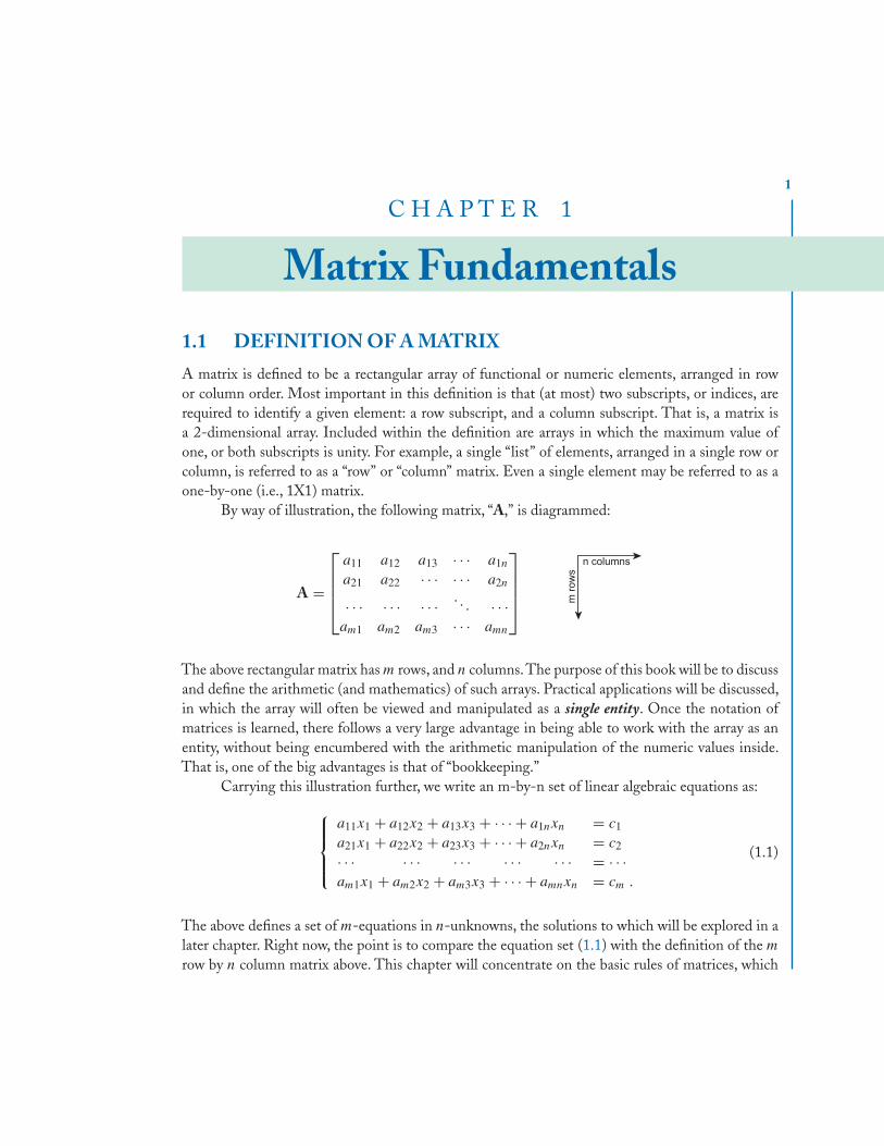
A matrix is defined to be a rectangular array of functional or numeric elements, arranged in rowor column order. Most important in this definition is that (at most) two subscripts, or indices, arerequired to identify a given element: a row subscript, and a column subscript. That is, a matrix isa 2-dimensional array. Included within the definition are arrays in which the maximum value ofone, or both subscripts is unity. For example, a single “list” of elements, arranged in a single row orcolumn, is referred to as a “row” or “column” matrix. Even a single element may be referred to as aone-by-one (i.e., 1X1) matrix.
By way of illustration, the following matrix, “A,” is diagrammed:
A =
⎡⎢⎢⎢⎣
a11 a12 a13 · · · a1n
a21 a22 · · · · · · a2n
· · · · · · · · · . . . · · ·am1 am2 am3 · · · amn
⎤⎥⎥⎥⎦
The above rectangular matrix has m rows, and n columns.The purpose of this book will be to discussand define the arithmetic (and mathematics) of such arrays. Practical applications will be discussed,in which the array will often be viewed and manipulated as a single entity. Once the notation ofmatrices is learned, there follows a very large advantage in being able to work with the array as anentity, without being encumbered with the arithmetic manipulation of the numeric values inside.That is, one of the big advantages is that of “bookkeeping.”
Carrying this illustration further, we write an m-by-n set of linear algebraic equations as:
⎧⎪⎪⎨⎪⎪⎩
a11x1 + a12x2 + a13x3 + · · · + a1nxn = c1
a21x1 + a22x2 + a23x3 + · · · + a2nxn = c2
· · · · · · · · · · · · · · · = · · ·am1x1 + am2x2 + am3x3 + · · · + amnxn = cm .
(1.1)
The above defines a set of m-equations in n-unknowns, the solutions to which will be explored in alater chapter. Right now, the point is to compare the equation set (1.1) with the definition of the m
row by n column matrix above. This chapter will concentrate on the basic rules of matrices, which
2 1. MATRIX FUNDAMENTALS
will, among other things, allow us to write the set (1.1) as:
Ax = c (1.2)
wherein the A matrix has the form diagrammed above. In (1.2), each of the literal symbols representsa matrix. The A matrix is a rectangular one, with m rows, and n columns. The x matrix has n rowsand just one column. It is usually referred to as a “vector,” as is the matrix, c, which has m rows and,again, just one column. As mentioned earlier, x and c can also be called column matrices (or columnvectors).
It will be noted immediately that, although (1.2) is beautifully compact, it does not convey allthe information of (1.1). That is, (1.2) does not make the “dimensionality” clear: It is not evidentthat A is m rows by n columns. This information must come from the context of the discussion—afairly small price to pay.
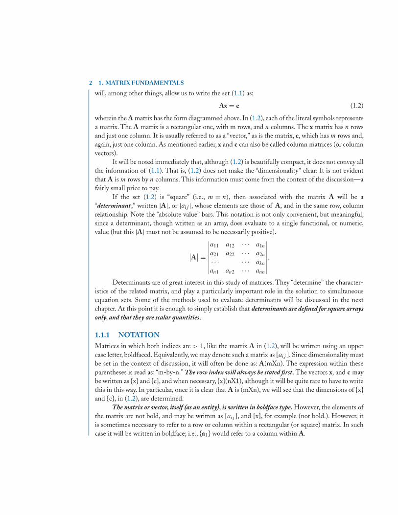
If the set (1.2) is “square” (i.e., m = n), then associated with the matrix A will be a“determinant ,” written |A|, or |aij |, whose elements are those of A, and in the same row, columnrelationship. Note the “absolute value” bars. This notation is not only convenient, but meaningful,since a determinant, though written as an array, does evaluate to a single functional, or numeric,value (but this |A| must not be assumed to be necessarily positive).
∣∣A∣∣ =
∣∣∣∣∣∣∣∣a11 a12 · · · a1n
a21 a22 · · · a2n
· · · · · · akn
an1 an2 · · · ann
∣∣∣∣∣∣∣∣.
Determinants are of great interest in this study of matrices. They “determine” the character-istics of the related matrix, and play a particularly important role in the solution to simultaneousequation sets. Some of the methods used to evaluate determinants will be discussed in the nextchapter. At this point it is enough to simply establish that determinants are defined for square arraysonly, and that they are scalar quantities.
1.1.1 NOTATIONMatrices in which both indices are > 1, like the matrix A in (1.2), will be written using an uppercase letter, boldfaced. Equivalently, we may denote such a matrix as [aij ]. Since dimensionality mustbe set in the context of discussion, it will often be done as: A(mXn). The expression within theseparentheses is read as: “m-by-n.” The row index will always be stated first . The vectors x, and c maybe written as {x} and {c}, and when necessary, {x}(nX1), although it will be quite rare to have to writethis in this way. In particular, once it is clear that A is (mXn), we will see that the dimensions of {x}and {c}, in (1.2), are determined.
The matrix or vector, itself (as an entity), is written in boldface type. However, the elements ofthe matrix are not bold, and may be written as [aij ], and {x}, for example (not bold.). However, itis sometimes necessary to refer to a row or column within a rectangular (or square) matrix. In suchcase it will be written in boldface; i.e., {a1} would refer to a column within A.
1.2. ELEMETARY MATRIX ALGEBRA 3
The {x} and {c} vectors in (1.2) are “column” vectors.There can also, be cases in which the rowdimension is unity: a (1Xn) vector. Such a vector is called a “row” vector. It will be written withintext as [v]. Please be careful to note the difference between [v] and {v}. For example, if we were toselect vectors from the matrix A, the row vectors would have n elements, but the column vectorswould have m elements—a very significant difference. Notice also that [v] (a row vector) will not beconfused with [aij ] (a rectangular matrix).
Within a text discussion, it would be very unwieldy to write the elements of a column vectorvertically down the page. Therefore, if the elements of either a row or column vector must bedelineated, it will be done across the page (“horizontally”). A three element column vector, {v},would be written as: {v1, v2, v3}. ⎧⎨
⎩v1
v2
v3
⎫⎬⎭ written as v or
{v1, v2, v3}
A three element row vector would be written [u1, u2, u3], with square brackets.Some notation examples, (numerical values chosen at random):
A = A(3X3) =⎡⎣ a11 a12 a13
a21 a22 a23
a31 a32 a33
⎤⎦ =
∥∥∥∥∥∥3.1 0 1.62.2 5.2 1.11.0 3.2 4.4
∥∥∥∥∥∥ . (1.3)
Note that a12 (for example) refers to the element in the first row and second column (in the exampleits value is 0).The row subscript is always given first . Ordinarily, the square brace, [. .], is the notationfor a matrix (while the single vertical bar denotes its determinant, |A|), but, notice that the doublevertical bar is sometimes used to denote a matrix.
As will be seen in coming chapters, a matrix is often viewed as an assemblage of vectors. Forexample, A in (1.3), may be viewed as three row vectors, [ak]. Note that the entity within the squarebraces must be shown bold, because it refers to a vector, (i.e., ak), not an element. A could also beviewed as three column vectors, {ak}. Note that the type of braces used distinguishes between a rowor a column vector. For example, with reference to (1.3):
[ a2] = [2.2 5.2 1.1
] ; {a2} = {0 5.2 3.2
}and, also note that {a2} is a column vector, but, is written across the page (for convenience). Withintext it would be written as { a2 } = { 0, 5.2, 3.2 }, with commas.
It is extremely difficult to strictly adhere to an unambiguous set of notation rules. Then, newrules, possibly contradictory, may be found throughout the book. The most important ‘rule’ is todescribe each topic clearly. Notation rules may sometimes be “bent” to fit the discussion.
1.2 ELEMETARY MATRIX ALGEBRAIn order to develop an elementary matrix algebra, the definitions of matrix equality, and the basicoperations of addition, and multiplication, must be agreed upon. It will be found that there are some
4 1. MATRIX FUNDAMENTALS
fundamental differences between matrix algebra and that of “ordinary” algebra, which deals with“scalar” entities—those ordinary numbers and functions whose dimension is 1X1. But, the rules ofmatrix algebra are logical, and will seem obvious rather than obtuse or complicated.
To begin, two matrices are equal iff (iff ≡“if and only if ”) the dimensions of each are thesame, and their corresponding elements are equal. For example, A = B iff they both have the samedimensions, mXn, and aij = bij , for all i and j .
1.2.1 ADDITION (INCLUDING SUBTRACTION)The sum of two (or more) matrices is formed by summing corresponding elements:
C = B ± A implies
[cij ] = [bij ] ± [aij ] . (1.4)
Note that if the two matrices are of different dimensionality then corresponding elements cannotbe found, in which case addition is not defined. Matrix addition is defined only when B and A havethe same numbers of rows and columns, respectively. When this is the case, the matrices A and B aresaid to be “conformable in addition.” If all the elements of A are respectively the negatives of thoseof B, then the sum, C, will have all zero elements. In such case, C is known as a “null” matrix (the“zero” of matrix algebra). Also, if A happened to be null, then C would be equal to B, cij = bij forall i and j .
Since addition is commutative for the elements of the matrix, then matrix addition itself iscommutative. That is, A + B = B + A.
1.2.2 MULTIPLICATION BY A SCALARThe matrix (k)A is formed by multiplying every element of A by the scalar (k). Note that thenotation (k), with parentheses, is used here. However, the notation, kA, will also be used. Neither(k)A, nor kA, will be confused with matrix multiplication, because row, or column, vectors (alsoexpressed in lower case) must be written as {k}, or [k]. In passing, we note that if A is square (nXn),and is multiplied by the scalar, k, then the determinant of A will be multiplied by kn. Conversely,then (k)|A| will mean the multiplication of a single row, or column, by k. More on this, later.
1.2.3 VECTOR MULTIPLICATIONSince rectangular matrices are composed of vectors, we will first discuss vector products, beforedefining the product of these “larger” matrices. The most important product of two vectors is their“dot product,” or “scalar product.” This product results in a scalar—just as does the vector dotproduct in vector analysis. Furthermore, the numerical result is the same also, since it is the sum of
1.2. ELEMETARY MATRIX ALGEBRA 5
the products of the corresponding elements.
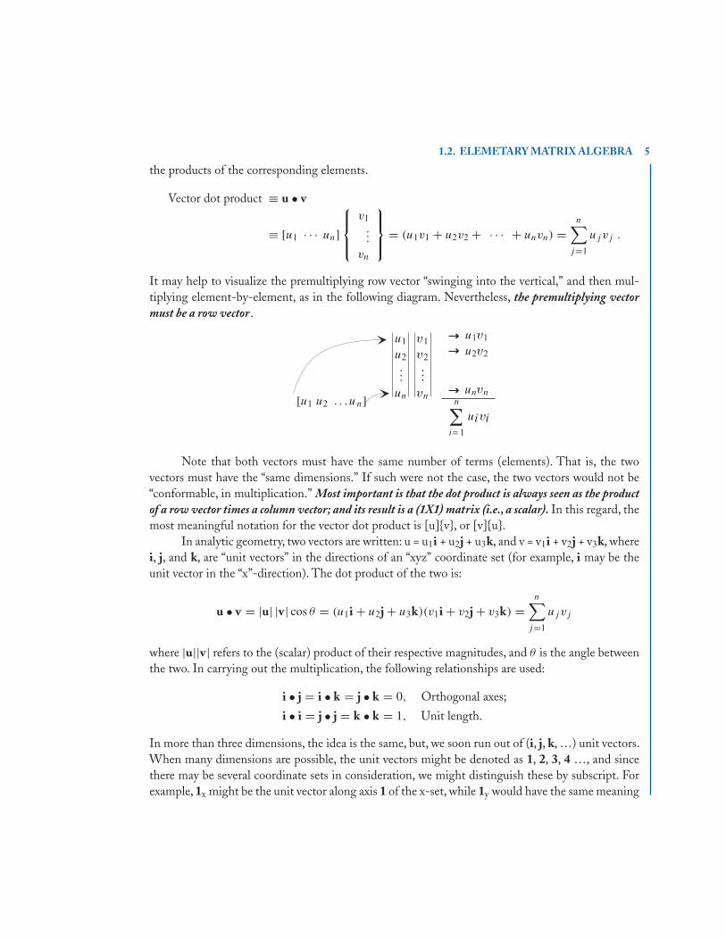
Vector dot product ≡ u • v
≡ [u1 · · · un]
⎧⎪⎨⎪⎩
v1...
vn
⎫⎪⎬⎪⎭ = (u1v1 + u2v2 + · · · + unvn) =
n∑j=1
ujvj .
It may help to visualize the premultiplying row vector “swinging into the vertical,” and then mul-tiplying element-by-element, as in the following diagram. Nevertheless, the premultiplying vectormust be a row vector.
...
=
Note that both vectors must have the same number of terms (elements). That is, the twovectors must have the “same dimensions.” If such were not the case, the two vectors would not be“conformable, in multiplication.” Most important is that the dot product is always seen as the productof a row vector times a column vector; and its result is a (1X1) matrix (i.e., a scalar). In this regard, themost meaningful notation for the vector dot product is [u]{v}, or [v]{u}.
In analytic geometry, two vectors are written: u = u1i + u2j + u3k, and v = v1i + v2j + v3k, wherei, j, and k, are “unit vectors” in the directions of an “xyz” coordinate set (for example, i may be theunit vector in the “x”-direction). The dot product of the two is:
u • v = |u| |v| cos θ = (u1i + u2j + u3k)(v1i + v2j + v3k) =n∑
j=1
ujvj
where |u||v| refers to the (scalar) product of their respective magnitudes, and θ is the angle betweenthe two. In carrying out the multiplication, the following relationships are used:
i • j = i • k = j • k = 0, Orthogonal axes;
i • i = j • j = k • k = 1, Unit length.
In more than three dimensions, the idea is the same, but, we soon run out of (i, j, k, …) unit vectors.When many dimensions are possible, the unit vectors might be denoted as 1, 2, 3, 4 …, and sincethere may be several coordinate sets in consideration, we might distinguish these by subscript. Forexample, 1x might be the unit vector along axis 1 of the x-set, while 1y would have the same meaning
6 1. MATRIX FUNDAMENTALS
in the y-set. More often, the vector is simply written {v1, v2, v3, …}. Although, we may have troublevisualizing vectors in more than 3 dimensions, we simply draw the analogy to the 3 dimensionalcase.
Note that, just as in 3 dimensions, the n-dimensional dot product can produce a zero resulteven when neither of the vectors is zero. That is, cos θ could be zero, in which case the vectors areperpendicular, or “orthogonal.”
The product v•v is always conformable, and is the sum of the squared elements of v. Again, byanalogy with 3 dimensions, v•v is the “square of the length” of v, and sqrt(v•v) is |v|, the “length”of the n dimensional vector. Also u•v is the product |u||v| multiplied by the cosine of the anglebetween u and v (as in vector analysis in 3 dimensions).
The product {v}[u] (a column vector times a row vector) is also conformable, when u and vhave the same dimensions. Given that both vectors are (nX1), the product is an (nXn) square matrix.This result will be reviewed again in the next paragraphs. See (1.21), Section 1.6.
1.2.4 MATRIX MULTIPLICATIONIn (1.2), the product Ax is set equal to the vector c. Apparently, then, the product of a rectangularmatrix and a vector is another vector. From (1.1), it will be seen that (in Ax=c) each (scalar) elementof c is the sum of the element-by-element products of a row vector of A by the column x: The first rowvector of A is: [a1] = [a11, a12, …, a1n]. The product [a1]{x} is c1, the first element of the vector c.That is (from (1.1)):
a11x1 + a12x2 + · · · + a1nxn = [a1]{x} =n∑
j=1
a1j xj = c1 .
The above equation is nothing more than a rewrite of the first equation in (1.1). But, theimportant point to get here is that the left side of the above is the dot product [a1]{x}. The conceptof matrix multiplication is simply the extension of this to the case where there are more columns inthe “post-”multiplier.
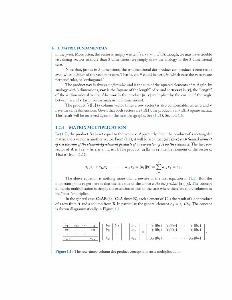
In the general case, C=AB (i.e., C=A times B), each element of C is the result of a dot productof a row from A and a column from B. In particular, the general element cij = ai • bj . The conceptis shown diagrammatically in Figure 1.1.
⎡⎢⎢⎢⎢⎣
a11 a12 · · · a1k
a21 · · · a2k
· · · · · · · · · · · ·am1 amk
⎤⎥⎥⎥⎥⎦⎡⎢⎢⎣
b11 b12 b1n
b21 · · · b2n
· · · · · · · · · · · ·bk1 bkn
⎤⎥⎥⎦ =
⎡⎢⎢⎣
[a1]{b1} [a1]{b2} · · · [a1]{bn}[a2]{b1} [a2]{b2} · · · [a2]{bn}
· · · · · ·[am]{b1} · · · · · · [am]{bn}
⎤⎥⎥⎦ .
Figure 1.1: The row-times-column dot product concept in matrix multiplicationn.
1.2. ELEMETARY MATRIX ALGEBRA 7
The figure is intended to emphasize the “row times column” dot product concept; so the Amatrix is shown “partitioned” into rows (by the horizontal lines), and the B matrix is partitionedinto columns. In the figure, the A matrix is shown with m rows, and k columns, i.e., A(mXk). The Bmatrix has k rows and n columns, B(kXn). The C matrix elements are all the results of a vector dotproduct. The following statements define matrix multiplication, and will clarify the dimensionalityof C.
• Each element of the product matrix, cij , is the result of the dot product [ai]{bj }.
cij = [ai]{bj } =k∑
s=1
aisbsj . (1.5)
• If the dot product [ai]{bj } is to be conformable, the number of terms in ai must be the sameas the number of terms in bj . Then the number of columns in A must equal the number of rowsin B. Thus, B must have k rows, conforming to the k columns in A.
• The conformability of AB does not depend on the number of rows of A, nor the number ofcolumns of B.
• As each succeeding row in A is selected (to form the next dot product), a new row is createdin the result, C. Then, C must have the same number of rows as A. The same reasoning showsthat C must have the same number of columns as B. Therefore, C is (mXn).
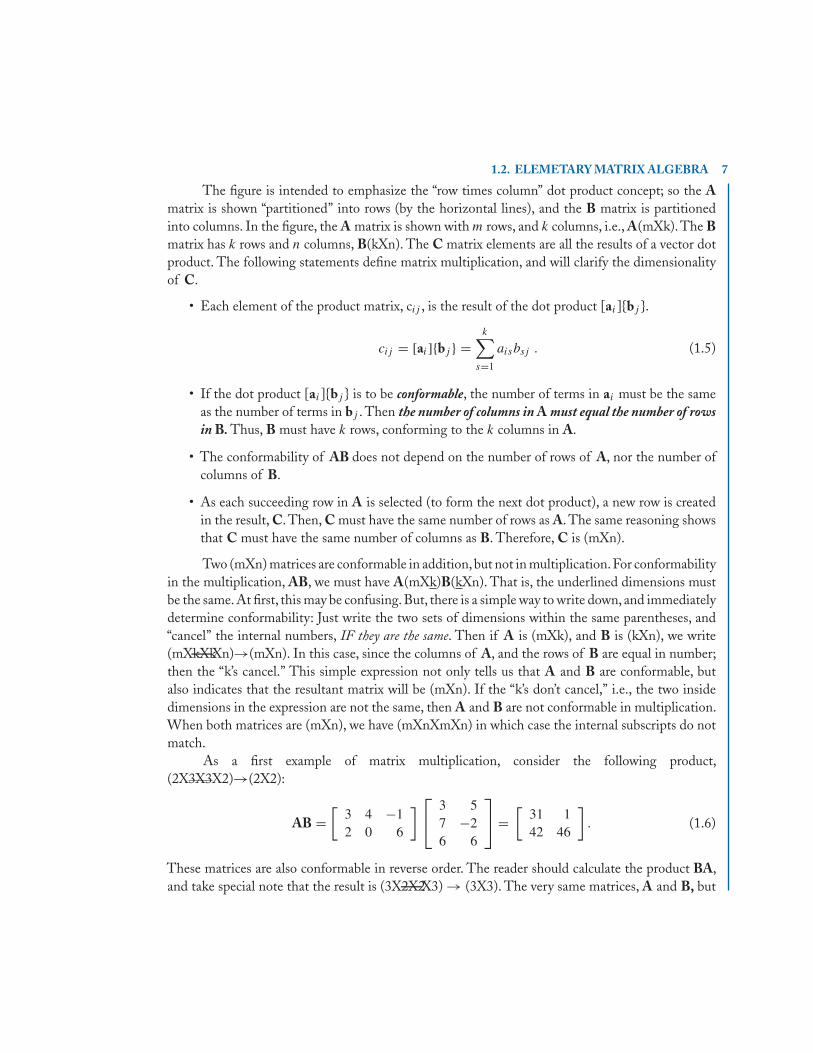
Two (mXn) matrices are conformable in addition,but not in multiplication.For conformabilityin the multiplication, AB, we must have A(mXk)B(kXn). That is, the underlined dimensions mustbe the same. At first, this may be confusing. But, there is a simple way to write down, and immediatelydetermine conformability: Just write the two sets of dimensions within the same parentheses, and“cancel” the internal numbers, IF they are the same. Then if A is (mXk), and B is (kXn), we write(mXkXk—–Xn)→(mXn). In this case, since the columns of A, and the rows of B are equal in number;then the “k’s cancel.” This simple expression not only tells us that A and B are conformable, butalso indicates that the resultant matrix will be (mXn). If the “k’s don’t cancel,” i.e., the two insidedimensions in the expression are not the same, then A and B are not conformable in multiplication.When both matrices are (mXn), we have (mXnXmXn) in which case the internal subscripts do notmatch.
As a first example of matrix multiplication, consider the following product,(2X3X3X2)→(2X2):
AB =[
3 4 −12 0 6
] ⎡⎣ 3 57 −26 6
⎤⎦ =
[31 142 46
]. (1.6)
These matrices are also conformable in reverse order. The reader should calculate the product BA,and take special note that the result is (3X2X2—–X3) → (3X3). The very same matrices, A and B, but
8 1. MATRIX FUNDAMENTALS
very different results—which illustrates thatmatrix multiplication is not commutative . That is, ingeneral AB �= BA.The product BA may not even be conformable in multiplication, even though ABis perfectly legal. For emphasis, however, please note that in general AB �= BA even if both productsare conformable. Try a few simple matrix products to prove that this is the case (We will see, shortly,that in some cases, multiplication is commutative).
Because of the non-commutative nature of the matrix product the order of the product, mustbe stated explicitly. For example, AB can be described as “the PREmultiplication of B, by A,” oralternatively, “the POST multiplication of A, by B.”
Matrix multiplication is, however, associative. That is:
A(BC) = (AB)C = ABC . (1.7)
It does not matter whether we form the product BC, first, then premultiply by A, or form AB, thenpostmultiply by C. Further, it is distributive:
A(B + C) = AB + AC . (1.8)
From (1.7), we may draw the inference that the powers of a (necessarily square) matrix, say A, aredefined: A2 = A(A), A3 = A(A)(A), and so on. Then, it follows that matrix polynomials are alsovalid:
p(A) = c0An + c1An−1 + · · · + cn−1A + cnI . (1.9)
In (1.9), the coefficients, ci , are scalar constants; cn multiplies the “unit matrix,” I, defined in Sec-tion 1.3, below.
Because matrix multiplication is so fundamental to our study, the reader should tryseveral examples, to become sure of the method. In each case, write the expressions like(2X3X3—–X2) to see how these indicate the conformability and the dimensions of the result.
1.2.5 TRANSPOSITIONThe matrix transpose of A is written A′ (“A prime”). A′ is obtained by interchanging the rows andcolumns of A. Then A(mXn) becomes A′(nXm) under transposition. Also, {v}′ => [v], that is, thetranspose of a column is a row, and vice versa. The transpose operation is very important. For clarity,it may sometimes be necessary to write A transpose as At , rather than A′.Transpose of a matrix product: Suppose C = AB, and we wish to express the transpose, C′, in termsof A′ and B′. Remember that the cij element of C is the dot product of the ith row of A into thej th column of B. Upon transposition, the columns of B become rows, and the rows of A becomecolumns. It therefore follows that in order to preserve the correct dot products, we must take the B′and A′ matrices in reverse order. That is:
C′ = (AB)′ = B′A′ ≡ Bt At . (1.10)
As a check, consider the 2,3 element of C′. It is the same as the 3,2 element of C. From (1.6),it is clear that the element c32 is obtained by [a3]{b2}. The element c′
23 is obtained by [b′2]{a′
3}.
1.3. BASIC TYPES OF MATRICES 9
Apparently then, the reasoning of (1.10) is correct. This is known as the “reversal rule” of matrixtransposition. By logical extension of this rule, to continued products:
D′ = (ABC)′ = (C)′(AB)′ = C′B′A′ . (1.11)
Note that for any matrix, A(mXn), that if B = A′A′, then B′ = B = A′A. That is, B is unchangedunder transposition. Such a matrix is called “symmetric.” See the next section, below.
1.3 BASIC TYPES OF MATRICES
1.3.1 THE UNIT MATRIXA square (nXn) matrix whose ij elements are zero for i �= j , and whose elements ii are unity, isdefined as the “unit matrix,” I. I corresponds to unity in scalar mathematics. For example, if they areconformable, I{x} = {x}, or AI =A. Just as in scalar algebra, the multiplication of a matrix, A(nXn),by the unit matrix, I(nXn), leaves A unaltered. Further, I commutes with any square matrix of thesame dimensions (i.e., IA = AI = A). Note also that I = I(I), and I′ = I.
In the unit matrix, I, the unity elements are said to lie in the “principal diagonal,” or the “maindiagonal.” The “off-diagonal” elements are zero.
The unit matrix can also be written as [δij ]. The symbol, “δij ,” is known as the “KroneckerDelta.” By definition, δij = 1, for i = j , and δij = 0, for i �= j .
1.3.2 THE DIAGONAL MATRIXIf the main diagonal elements are not unity, but all elements off this diagonal are zero, then thematrix is a “diagonal matrix.” The diagonal elements are not, in general, equal in value. In the casesin which the main diagonal elements are equal, the matrix is called a “scalar matrix.” (In the matrixpolynomial, written above, (1.9), cnI is a scalar matrix.)
The product of two diagonal matrices is another diagonal matrix, whose main diagonal el-ements are the products of the corresponding elements of the two given matrices. Clearly, then,diagonal matrix products commute. However, if A is not diagonal, and B is diagonal, the product isnot commutative. In BA, the corresponding rows of A are multiplied by the diagonal elements ofB, while in AB, the corresponding columns of A are multiplied by the diagonal elements of B. Tryboth cases, to be assured that this is true.
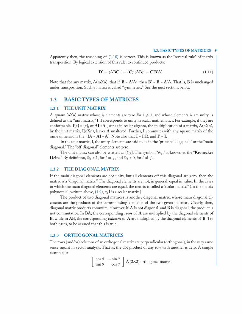
1.3.3 ORTHOGONAL MATRICESThe rows (and/or) columns of an orthogonal matrix are perpendicular (orthogonal), in the very samesense meant in vector analysis. That is, the dot product of any row with another is zero. A simpleexample is: [
cos θ − sin θ
sin θ cos θ
]A (2X2) orthogonal matrix.
10 1. MATRIX FUNDAMENTALS
Clearly, the rows and columns of the above 2X2 are orthogonal; their dot products are zero. Inthe case of this example, the matrix is also said to be “orthonormal,” because the lengths of therows/columns are normalized to 1.0 (i.e., the dot product of any row/column into itself is 1.0). Theorthogonal matrix has frequent application in engineering problems.
Given an nXn orthonormal matrix, A, it should be clear that A′A = I, the unit matrix, becauseA′A simply forms all the dot products of the columns of A with each other. Only when a columnis dotted into itself is there a nonzero result, and that result will lie on the main diagonal, and willhave the value unity. More generally, if A is just orthogonal (not normalized), then a diagonal matrixresults from the A′A product.
1.3.4 TRIANGULAR MATRICESIf the matrix, A, has all zero elements below the main diagonal, it is known as an “upper triangular”matrix. The transpose of an upper triangular matrix—one with all zero elements above the maindiagonal—is called “lower triangular.”
Such matrices are very important because (1) their determinant is easily calculated as theproduct of its main diagonal terms, and (2) its inverse is similarly easy to determine. The followingexample (though not a matrix inversion) indicates the ease of solution of a triagular set of equations:⎡
⎣ 1 2 −10 3 30 0 5
⎤⎦⎧⎨⎩
x1
x2
x3
⎫⎬⎭ =
⎧⎨⎩
795
⎫⎬⎭ .
Since the last equation is “uncoupled,” x3 = 1 by inspection. Once x3 is known, x2 can be solved,and then x1 follows.
It is not surprising that many methods for solving determinants, equation sets, and matrixinversions incorporate matrix triangularization.
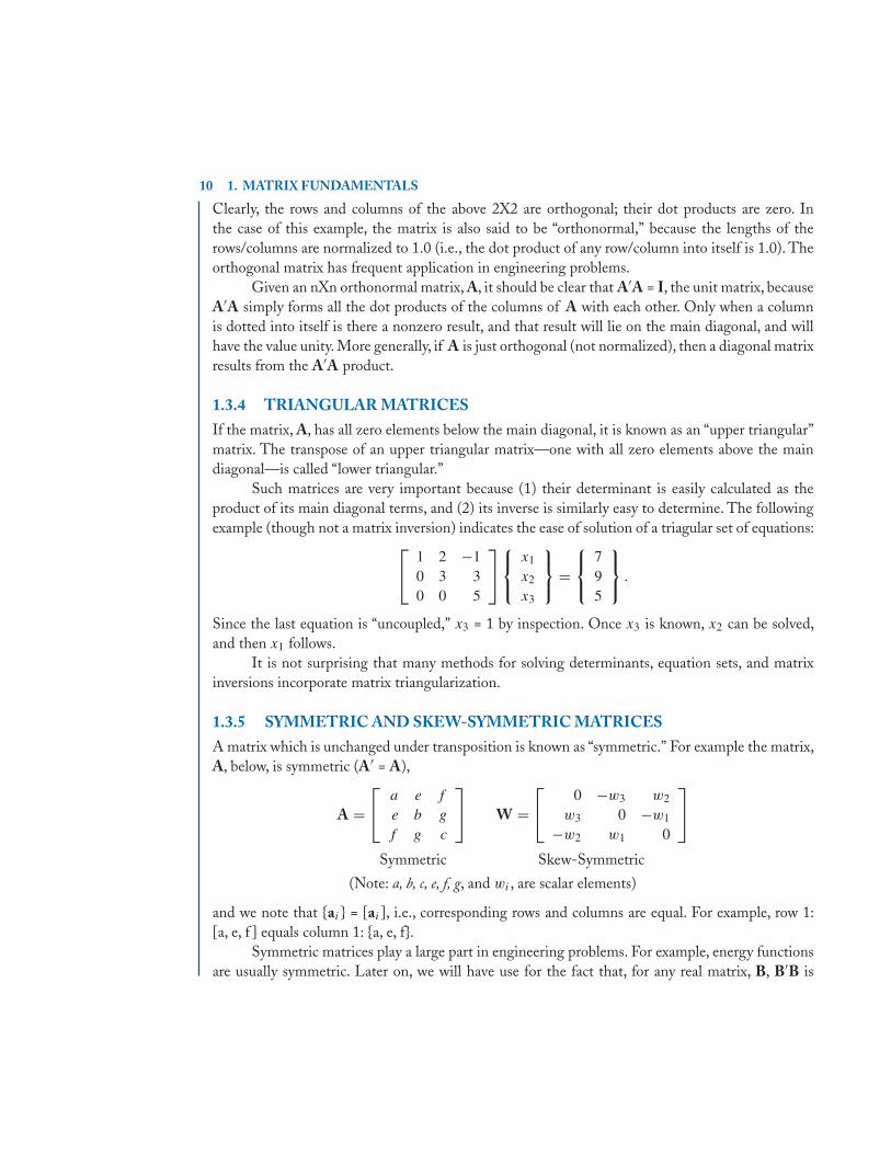
1.3.5 SYMMETRIC AND SKEW-SYMMETRIC MATRICESA matrix which is unchanged under transposition is known as “symmetric.” For example the matrix,A, below, is symmetric (A′ = A),
A =⎡⎣ a e f
e b g
f g c
⎤⎦ W =
⎡⎣ 0 −w3 w2
w3 0 −w1
−w2 w1 0
⎤⎦
Symmetric Skew-Symmetric
(Note: a, b, c, e, f, g, and wi , are scalar elements)
and we note that {ai} = [ai], i.e., corresponding rows and columns are equal. For example, row 1:[a, e, f ] equals column 1: {a, e, f}.
Symmetric matrices play a large part in engineering problems. For example, energy functionsare usually symmetric. Later on, we will have use for the fact that, for any real matrix, B, B′B is
1.3. BASIC TYPES OF MATRICES 11
always a square, symmetric matrix. That is, in general, B is (mXn), and the product (nXmXmXn) is(nXn), i.e., square. It is obvious that (B′B)′ = B′B, i.e., the product matrix is symmetric.
If W′ = −W, then W is called a “Skew-symmetric matrix.” Since the principal diagonalelements are unchanged under transposition, then necessarily, the main diagonal elements of askew-symmetric matrix must be zero. The most prominent example of a skew-symmetric matrix isthe angular velocity matrix (Chapter 5).
1.3.6 COMPLEX MATRICESA matrix, Z, whose elements are complex numbers can be written [zij ], where zij = xij + jyij , orZ = X + jY, (where “j ” is the notation for
√−1). The latter form shows a “separation” of the realand imaginary parts into separate matrices. In this notation, both X and Y , are composed of realnumbers. A matrix, W = X − jY, is called the “conjugate” of Z. The transpose of W is referred toas the “associate” of Z.
The sum,or product,of two complex matrices can be formed in the straightforward,element byelement, way—using complex arithmetic—or using the second notation, (Z = X + jY ), previouslycoded (real arithmetic) routines can be used, since X and Y are composed of real numbers. Forexample:
Z1Z2 = (X1X2 − Y1Y2) + j (X1Y2 + Y1X2) .
The Hermitian matrix: If the elements of the complex matrix, Z = X + jY, are such that X is symmetric,and Y is skew symmetric, then Z is known as an “Hermitian” matrix. The Hermitian matrix is equalto its “associate.” That is, if Z is Hermitian, then Z is equal to the conjugate of its transpose. TheHermitian matrix (with its symmetrical real part) is similar in ways to the (entirely real) symmetricmatrix.
1.3.7 THE INVERSE MATRIXThus, far, we have not defined matrix division. In the general case, no such operation as A/B exists.However, if A is a square matrix, then there may be a matrix, B, such that AB = I. In this case,the matrix B is referred to as the “inverse” of A, and is written with −1 in superscript as B = A−1.Similarly, A = B−1. The notation A/B or A = 1/B is never used.
The matrices, A and B, shown below, are examples:
A =⎡⎣1 2 2
1 0 11 −3 0
⎤⎦ B =
⎡⎣−3 6 −2
−1 2 −13 −5 2
⎤⎦ AB =
⎡⎣1 0 0
0 1 00 0 1
⎤⎦
and, since AB = BA then B = A−1, and A = B−1.Note that inverse matrices commute (i.e., AA−1 = A−1A). Using the example, prove that this
is true by multiplying AB and then BA to show that they are the same.
12 1. MATRIX FUNDAMENTALS
Finding the solution to a (square) set of linear algebraic equations (when the solution is unique)is equivalent to finding the inverse of the coefficient matrix:
Given Ax = c, then(A−1)Ax = (A−1)c; assuming that A−1 exists. (1.12)
x = (A−1)c
Not every matrix has an inverse. For example, an nXm (non-square) matrix does not. Some square(nXn) matrices do not have an inverse. Those that do not are called “singular matrices.”
The inverse of a diagonal matrix is another diagonal matrix, whose principal diagonal elementsare the reciprocals of the corresponding elements of the given matrix. Clearly, then, a diagonal matrixwith a zero element on the main diagonal, is “singular.”
Also, the transpose of an inverse matrix is equal to the inverse of its transpose. That is, givena “non-singular” matrix, A:
A(A−1) = Ithen (A(A−1))′ = (I)′ = I
(A−1)′A′ = I
and, by postmultiplying by the inverse of A-transpose, (A′)−1:
(A−1)′ = (A′)−1 .
The above equation shows not only the proof of the above statement, it also shows that the inverseof a symmetric matrix is also symmetric.
By similar reasoning, consider the matrix product, C = AB. Postmultiplying by B−1
CB−1 = A .
Now, postmultiply by A−1:C(B−1A−1) = I .
Then, C−1 must be equal to the product B−1A−1. That is, the reversal rule applies to the productof matrices: The inverse of the product of two matrices is equal to the product of their individualinverses, taken in the reverse order. This fact is sometimes referred to as the “reversal rule” of matrixmultiplication. It is worth reviewing that this reverse order phenomenon was also found in formingthe transpose of the product of two matrices, (1.10).
1.4 TRANSFORMATION MATRICESIt is frequently necessary to manipulate rows, columns, elements within a matrix. Section 3.2 ofChapter 3 discusses three “Elementary Operations” that are useful in diagonalizing a matrix. These
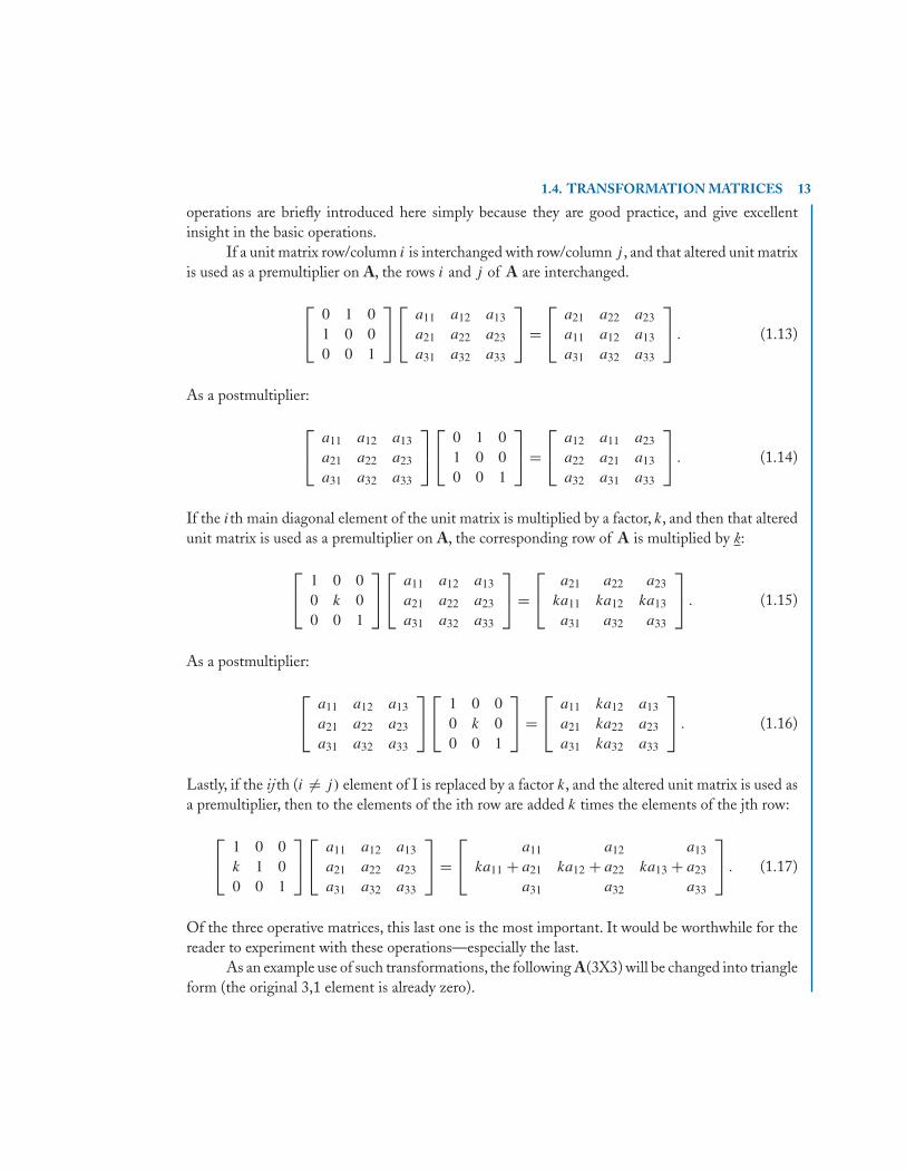
1.4. TRANSFORMATION MATRICES 13
operations are briefly introduced here simply because they are good practice, and give excellentinsight in the basic operations.
If a unit matrix row/column i is interchanged with row/column j , and that altered unit matrixis used as a premultiplier on A, the rows i and j of A are interchanged.
⎡⎣ 0 1 0
1 0 00 0 1
⎤⎦⎡⎣ a11 a12 a13
a21 a22 a23
a31 a32 a33
⎤⎦ =
⎡⎣ a21 a22 a23
a11 a12 a13
a31 a32 a33
⎤⎦ . (1.13)
As a postmultiplier:
⎡⎣ a11 a12 a13
a21 a22 a23
a31 a32 a33
⎤⎦⎡⎣ 0 1 0
1 0 00 0 1
⎤⎦ =
⎡⎣ a12 a11 a23
a22 a21 a13
a32 a31 a33
⎤⎦ . (1.14)
If the ith main diagonal element of the unit matrix is multiplied by a factor, k, and then that alteredunit matrix is used as a premultiplier on A, the corresponding row of A is multiplied by k:
⎡⎣ 1 0 0
0 k 00 0 1
⎤⎦⎡⎣ a11 a12 a13
a21 a22 a23
a31 a32 a33
⎤⎦ =
⎡⎣ a21 a22 a23
ka11 ka12 ka13
a31 a32 a33
⎤⎦ . (1.15)
As a postmultiplier:
⎡⎣ a11 a12 a13
a21 a22 a23
a31 a32 a33
⎤⎦⎡⎣ 1 0 0
0 k 00 0 1
⎤⎦ =
⎡⎣ a11 ka12 a13
a21 ka22 a23
a31 ka32 a33
⎤⎦ . (1.16)
Lastly, if the ijth (i �= j) element of I is replaced by a factor k, and the altered unit matrix is used asa premultiplier, then to the elements of the ith row are added k times the elements of the jth row:
⎡⎣ 1 0 0
k 1 00 0 1
⎤⎦⎡⎣ a11 a12 a13
a21 a22 a23
a31 a32 a33
⎤⎦ =
⎡⎣ a11 a12 a13
ka11 + a21 ka12 + a22 ka13 + a23
a31 a32 a33
⎤⎦ . (1.17)
Of the three operative matrices, this last one is the most important. It would be worthwhile for thereader to experiment with these operations—especially the last.
As an example use of such transformations, the following A(3X3) will be changed into triangleform (the original 3,1 element is already zero).
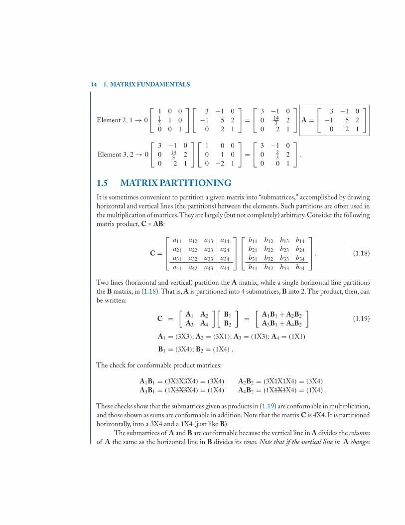
14 1. MATRIX FUNDAMENTALS
Element 2, 1 → 0
⎡⎣ 1 0 0
13 1 00 0 1
⎤⎦⎡⎣ 3 −1 0
−1 5 20 2 1
⎤⎦ =
⎡⎣ 3 −1 0
0 143 2
0 2 1
⎤⎦ A =
⎡⎣ 3 −1 0
−1 5 20 2 1
⎤⎦
Element 3, 2 → 0
⎡⎣ 3 −1 0
0 143 2
0 2 1
⎤⎦⎡⎣ 1 0 0
0 1 00 −2 1
⎤⎦ =
⎡⎣ 3 −1 0
0 23 2
0 0 1
⎤⎦ .
1.5 MATRIX PARTITIONINGIt is sometimes convenient to partition a given matrix into “submatrices,” accomplished by drawinghorizontal and vertical lines (the partitions) between the elements. Such partitions are often used inthe multiplication of matrices.They are largely (but not completely) arbitrary. Consider the followingmatrix product, C = AB:
C =
⎡⎢⎢⎣
a11 a12 a13 a14
a21 a22 a23 a24
a31 a32 a33 a34
a41 a42 a43 a44
⎤⎥⎥⎦⎡⎢⎢⎣
b11 b12 b13 b14
b21 b22 b23 b24
b31 b32 b33 b34
b41 b42 b43 b44
⎤⎥⎥⎦ . (1.18)
Two lines (horizontal and vertical) partition the A matrix, while a single horizontal line partitionsthe B matrix, in (1.18). That is, A is partitioned into 4 submatrices, B into 2. The product, then, canbe written:
C =[
A1 A2
A3 A4
] [B1
B2
]=
[A1B1 + A2B2
A3B1 + A4B2
](1.19)
A1 = (3X3); A2 = (3X1); A3 = (1X3); A4 = (1X1)
B1 = (3X4); B2 = (1X4) .
The check for conformable product matrices:
A1B1 = (3X3X3X4) = (3X4) A2B2 = (3X1X1X4) = (3X4)
A3B1 = (1X3X3X4) = (1X4) A4B2 = (1X1X1X4) = (1X4) .
These checks show that the submatrices given as products in (1.19) are conformable in multiplication,and those shown as sums are conformable in addition. Note that the matrix C is 4X4. It is partitionedhorizontally, into a 3X4 and a 1X4 (just like B).
The submatrices of A and B are conformable because the vertical line in A divides the columnsof A the same as the horizontal line in B divides its rows. Note that if the vertical line in A changes
1.5. MATRIX PARTITIONING 15
position, it forces the line in B to change position. But, the horizontal line, in A is arbitrary. It can bemoved anywhere without destroying conformability.
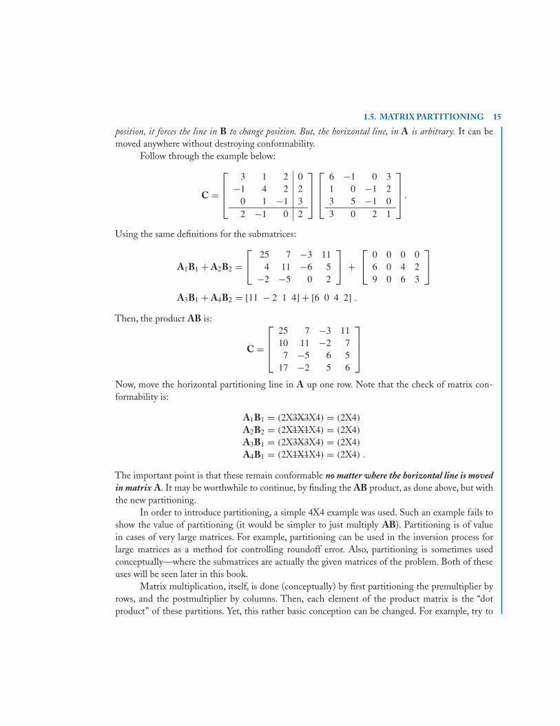
Follow through the example below:
C =
⎡⎢⎢⎣
3 1 2 0−1 4 2 2
0 1 −1 32 −1 0 2
⎤⎥⎥⎦⎡⎢⎢⎣
6 −1 0 31 0 −1 23 5 −1 03 0 2 1
⎤⎥⎥⎦ .
Using the same definitions for the submatrices:
A1B1 + A2B2 =⎡⎣ 25 7 −3 11
4 11 −6 5−2 −5 0 2
⎤⎦ +
⎡⎣ 0 0 0 0
6 0 4 29 0 6 3
⎤⎦
A3B1 + A4B2 = [11 − 2 1 4] + [6 0 4 2] .
Then, the product AB is:
C =
⎡⎢⎢⎣
25 7 −3 1110 11 −2 7
7 −5 6 517 −2 5 6
⎤⎥⎥⎦
Now, move the horizontal partitioning line in A up one row. Note that the check of matrix con-formability is:
A1B1 = (2X3X3X4) = (2X4)
A2B2 = (2X1X1X4) = (2X4)
A3B1 = (2X3X3X4) = (2X4)
A4B1 = (2X1X1X4) = (2X4) .
The important point is that these remain conformable no matter where the horizontal line is movedin matrix A. It may be worthwhile to continue, by finding the AB product, as done above, but withthe new partitioning.
In order to introduce partitioning, a simple 4X4 example was used. Such an example fails toshow the value of partitioning (it would be simpler to just multiply AB). Partitioning is of valuein cases of very large matrices. For example, partitioning can be used in the inversion process forlarge matrices as a method for controlling roundoff error. Also, partitioning is sometimes usedconceptually—where the submatrices are actually the given matrices of the problem. Both of theseuses will be seen later in this book.
Matrix multiplication, itself, is done (conceptually) by first partitioning the premultiplier byrows, and the postmultiplier by columns. Then, each element of the product matrix is the “dotproduct” of these partitions. Yet, this rather basic conception can be changed. For example, try to
16 1. MATRIX FUNDAMENTALS
visualize the premultiplier partitioned into columns and the postmultiplier in rows—in, say, an nXnproduct. Now, each (of the n) column times row products yields an nXn matrix; the sum of these n
products produces the end result.Finally, please note that partitioning is here referred to product matrices. It should be clear
that partitioning for addition (somewhat trivial) would be quite different. For example, none of thematrices above are partitioned to be conformable in addition (i.e., for A + B = C).
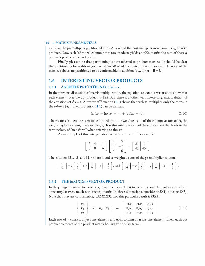
1.6 INTERESTING VECTOR PRODUCTS1.6.1 AN INTERPRETATION OF Ax = cIn the previous discussion of matrix multiplication, the equation set Ax = c was used to show thateach element ci is the dot product [ai]{x}. But, there is another, very interesting, interpretation ofthe equation set Ax = c. A review of Equation (1.1) shows that each xi multiplies only the terms inthe column {ai}. Then, Equation (1.1) can be written:
{a1}x1 + {a2}x2 + · · · + {an}xn = {c} . (1.20)
The vector c is therefore seen to be formed from the weighted sum of the column vectors of A, theweighting factors being the variables, xi . It is this interpretation of the equation set that leads to theterminology of “transform” when referring to the set.
As an example of this interpretation, we return to an earlier example
[3 4 −12 0 6
] ⎡⎣ 3 57 −26 6
⎤⎦ =
[31 142 46
].
The columns {31, 42} and {1, 46} are found as weighted sums of the premultiplier columns:{3142
}= 3
{32
}+ 7
{40
}+ 6
{ −16
}, and
{1
46
}= 5
{32
}− 2
{40
}+ 6
{ −16
}.
1.6.2 THE (nX1X1Xn) VECTOR PRODUCTIn the paragraph on vector products, it was mentioned that two vectors could be multiplied to forma rectangular (very much non-vector) matrix. In three dimensions, consider v(3X1) times u(1X3).Note that they are conformable, (3X1X1X3), and this particular result is (3X3):⎧⎨
⎩v1
v2
v3
⎫⎬⎭[
u1 u2 u3] =
⎡⎣ v1u1 v1u2 v1u3
v2u1 v2u2 v2u3
v3u1 v3u2 v3u3
⎤⎦ . (1.21)
Each row of v consists of just one element, and each column of u has one element. Then, each dotproduct elements of the product matrix has just the one vu term.
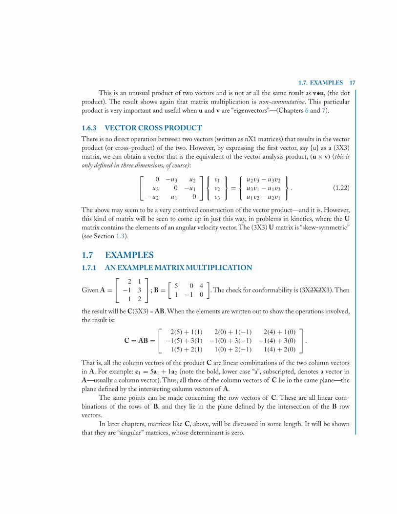
1.7. EXAMPLES 17
This is an unusual product of two vectors and is not at all the same result as v•u, (the dotproduct). The result shows again that matrix multiplication is non-commutative. This particularproduct is very important and useful when u and v are “eigenvectors”—(Chapters 6 and 7).
1.6.3 VECTOR CROSS PRODUCTThere is no direct operation between two vectors (written as nX1 matrices) that results in the vectorproduct (or cross-product) of the two. However, by expressing the first vector, say {u} as a (3X3)matrix, we can obtain a vector that is the equivalent of the vector analysis product, (u × v) (this isonly defined in three dimensions, of course):⎡
⎣ 0 −u3 u2
u3 0 −u1
−u2 u1 0
⎤⎦⎧⎨⎩
v1
v2
v3
⎫⎬⎭ =
⎧⎨⎩
u2v3 − u3v2
u3v1 − u1v3
u1v2 − u2v1
⎫⎬⎭ . (1.22)
The above may seem to be a very contrived construction of the vector product—and it is. However,this kind of matrix will be seen to come up in just this way, in problems in kinetics, where the Umatrix contains the elements of an angular velocity vector. The (3X3) U matrix is “skew-symmetric”(see Section 1.3).
1.7 EXAMPLES1.7.1 AN EXAMPLE MATRIX MULTIPLICATION
Given A =⎡⎣ 2 1
−1 31 2
⎤⎦ ; B =
[5 0 41 −1 0
]. The check for conformability is (3X2X2X3). Then
the result will be C(3X3) = AB. When the elements are written out to show the operations involved,the result is:
C = AB =⎡⎣ 2(5) + 1(1) 2(0) + 1(−1) 2(4) + 1(0)
−1(5) + 3(1) −1(0) + 3(−1) −1(4) + 3(0)
1(5) + 2(1) 1(0) + 2(−1) 1(4) + 2(0)
⎤⎦ .
That is, all the column vectors of the product C are linear combinations of the two column vectorsin A. For example: c1 = 5a1 + 1a2 (note the bold, lower case “a”, subscripted, denotes a vector inA—usually a column vector). Thus, all three of the column vectors of C lie in the same plane—theplane defined by the intersecting column vectors of A.
The same points can be made concerning the row vectors of C. These are all linear com-binations of the rows of B, and they lie in the plane defined by the intersection of the B rowvectors.
In later chapters, matrices like C, above, will be discussed in some length. It will be shownthat they are “singular” matrices, whose determinant is zero.
18 1. MATRIX FUNDAMENTALS
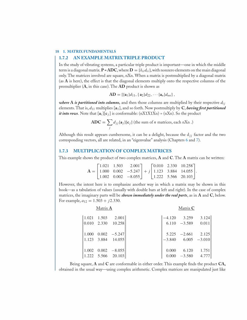
1.7.2 AN EXAMPLE MATRIX TRIPLE PRODUCTIn the study of vibrating systems, a particular triple product is important—one in which the middleterm is a diagonal matrix. P = ADC,where D = [δiidii],with nonzero elements on the main diagonalonly. The matrices involved are square, nXn. When a matrix is postmultiplied by a diagonal matrix(as A is here), the effect is that the diagonal elements multiply onto the respective columns of thepremultiplier (A, in this case). The AD product is shown as
AD = [{a1}d11, { a2}d22, · · · {an}dnn] ,
where A is partitioned into columns, and then those columns are multiplied by their respective dij
elements. That is, d11 multiplies {a1}, and so forth. Now postmultiply by C, having first partitionedit into rows. Note that {ai}[cj ] is conformable: (nX1X1Xn) = (nXn). So the product
ADC =∑j
djj {aj }[cj ] (the sum of n matrices, each nXn .)
Although this result appears cumbersome, it can be a delight, because the djj factor and the twocorresponding vectors, all are related, in an “eigenvalue” analysis (Chapters 6 and 7).
1.7.3 MULTIPLICATION OF COMPLEX MATRICESThis example shows the product of two complex matrices, A and C. The A matrix can be written:
A =⎡⎣1.021 1.503 2.001
1.000 0.002 −5.2471.002 0.002 −8.055
⎤⎦+ j
⎡⎣0.010 2.330 10.258
1.123 3.884 14.0551.222 5.566 20.103
⎤⎦.
However, the intent here is to emphasize another way in which a matrix may be shown in thisbook—as a tabulation of values (usually with double bars at left and right). In the case of complexmatrices, the imaginary parts will be shown immediately under the real parts, as in A and C, below.For example, a12 = 1.503 + j2.330.
Matrix A∥∥∥∥∥∥∥∥∥∥∥∥∥∥∥∥∥
1.021 1.503 2.0010.010 2.330 10.258
1.000 0.002 −5.2471.123 3.884 14.055
1.002 0.002 −8.0551.222 5.566 20.103
∥∥∥∥∥∥∥∥∥∥∥∥∥∥∥∥∥
Matrix C∥∥∥∥∥∥∥∥∥∥∥∥∥∥∥∥∥
−4.120 3.259 3.1246.110 −3.589 0.011
5.225 −2.661 2.125−3.840 6.005 −3.010
0.000 6.120 1.7510.000 −3.580 4.777
∥∥∥∥∥∥∥∥∥∥∥∥∥∥∥∥∥Being square, A and C are conformable in either order. This example finds the product CA,
obtained in the usual way—using complex arithmetic. Complex matrices are manipulated just like
1.8. EXERCISES 19
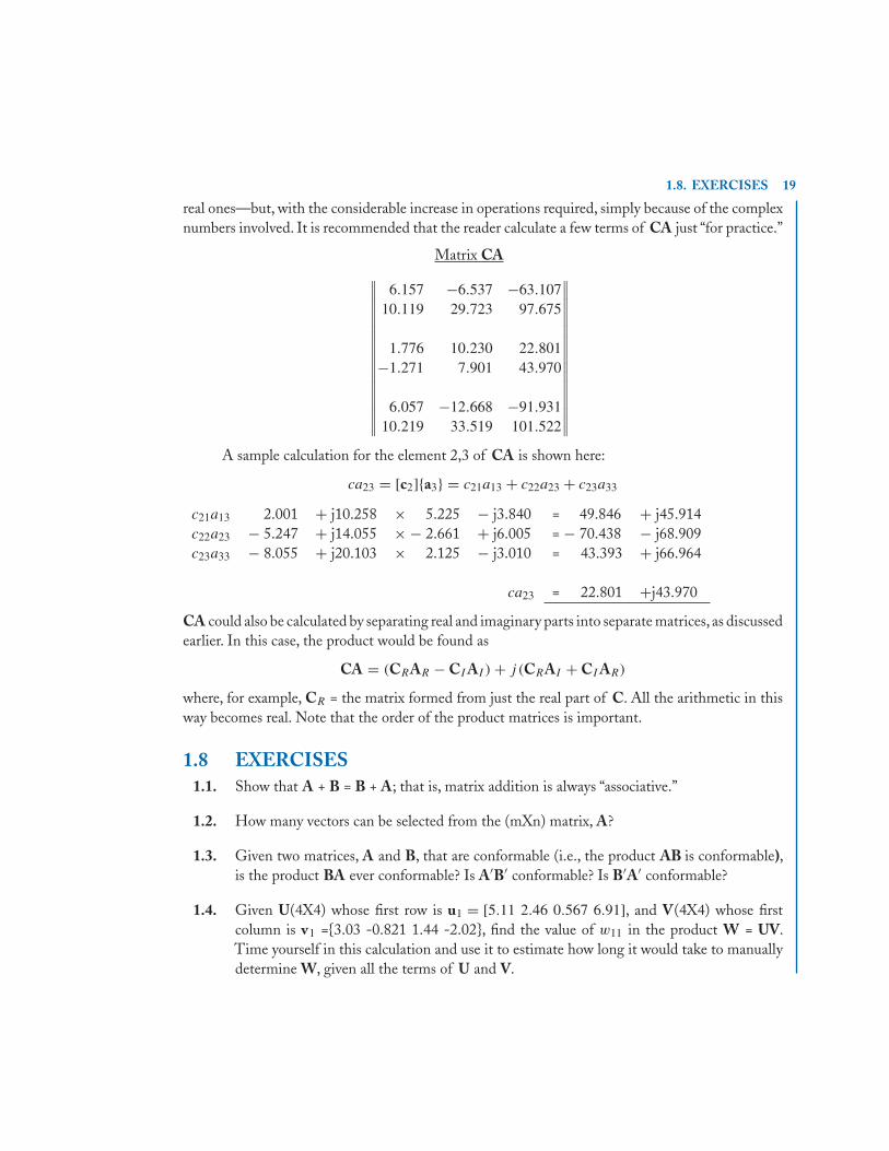
real ones—but, with the considerable increase in operations required, simply because of the complexnumbers involved. It is recommended that the reader calculate a few terms of CA just “for practice.”
Matrix CA∥∥∥∥∥∥∥∥∥∥∥∥∥∥∥∥∥
6.157 −6.537 −63.10710.119 29.723 97.675
1.776 10.230 22.801−1.271 7.901 43.970
6.057 −12.668 −91.93110.219 33.519 101.522
∥∥∥∥∥∥∥∥∥∥∥∥∥∥∥∥∥A sample calculation for the element 2,3 of CA is shown here:
ca23 = [c2]{a3} = c21a13 + c22a23 + c23a33
c21a13 2.001 + j10.258 × 5.225 − j3.840 = 49.846 + j45.914c22a23 − 5.247 + j14.055 × − 2.661 + j6.005 = − 70.438 − j68.909c23a33 − 8.055 + j20.103 × 2.125 − j3.010 = 43.393 + j66.964
ca23 = 22.801 +j43.970
CA could also be calculated by separating real and imaginary parts into separate matrices, as discussedearlier. In this case, the product would be found as
CA = (CRAR − CI AI ) + j (CRAI + CI AR)
where, for example, CR = the matrix formed from just the real part of C. All the arithmetic in thisway becomes real. Note that the order of the product matrices is important.
1.8 EXERCISES1.1. Show that A + B = B + A; that is, matrix addition is always “associative.”
1.2. How many vectors can be selected from the (mXn) matrix, A?
1.3. Given two matrices, A and B, that are conformable (i.e., the product AB is conformable),is the product BA ever conformable? Is A′B′ conformable? Is B′A′ conformable?
1.4. Given U(4X4) whose first row is u1 = [5.11 2.46 0.567 6.91], and V(4X4) whose firstcolumn is v1 ={3.03 -0.821 1.44 -2.02}, find the value of w11 in the product W = UV.Time yourself in this calculation and use it to estimate how long it would take to manuallydetermine W, given all the terms of U and V.
20 1. MATRIX FUNDAMENTALS
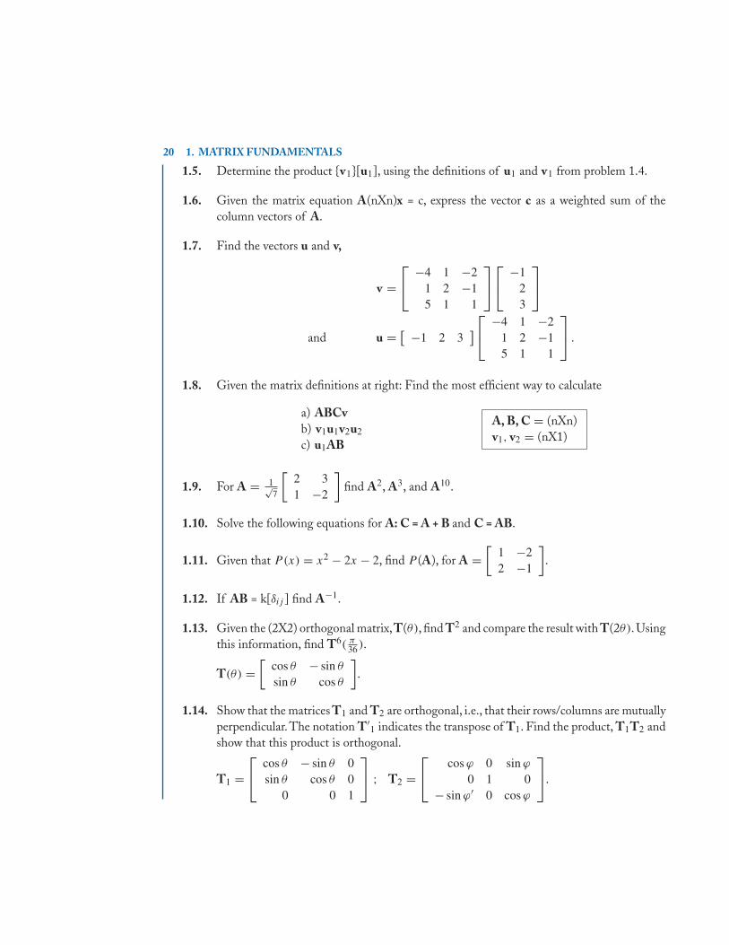
1.5. Determine the product {v1}[u1], using the definitions of u1 and v1 from problem 1.4.
1.6. Given the matrix equation A(nXn)x = c, express the vector c as a weighted sum of thecolumn vectors of A.
1.7. Find the vectors u and v,
v =⎡⎣ −4 1 −2
1 2 −15 1 1
⎤⎦⎡⎣ −1
23
⎤⎦
and u = [ −1 2 3]⎡⎣ −4 1 −2
1 2 −15 1 1
⎤⎦ .
1.8. Given the matrix definitions at right: Find the most efficient way to calculate
a) ABCvb) v1u1v2u2
c) u1AB
A, B, C = (nXn)v1, v2 = (nX1)
1.9. For A = 1√7
[2 31 −2
]find A2, A3, and A10.
1.10. Solve the following equations for A: C = A + B and C = AB.
1.11. Given that P(x) = x2 − 2x − 2, find P (A), for A =[
1 −22 −1
].
1.12. If AB = k[δij ] find A−1.
1.13. Given the (2X2) orthogonal matrix,T(θ), find T2 and compare the result with T(2θ). Usingthis information, find T6( π
36 ).
T(θ) =[
cos θ − sin θ
sin θ cos θ
].
1.14. Show that the matrices T1 and T2 are orthogonal, i.e., that their rows/columns are mutuallyperpendicular. The notation T′
1 indicates the transpose of T1. Find the product, T1T2 andshow that this product is orthogonal.
T1 =⎡⎣ cos θ − sin θ 0
sin θ cos θ 00 0 1
⎤⎦ ; T2 =
⎡⎣ cos ϕ 0 sin ϕ
0 1 0− sin ϕ′ 0 cos ϕ
⎤⎦.

1.8. EXERCISES 21
1.15. Find the product
⎡⎣ 1 1 1
1 1 11 1 1
⎤⎦⎡⎣ 3 6 4
−2 3 −50 −8 1
⎤⎦.
1.16. In the matrix product P = ABC show that pij = [ai]B{cj }.
1.17. Given the (4X4) matrix [aij ], determine an elementary transformation matrix that willcause element a31 to vanish (go to zero).

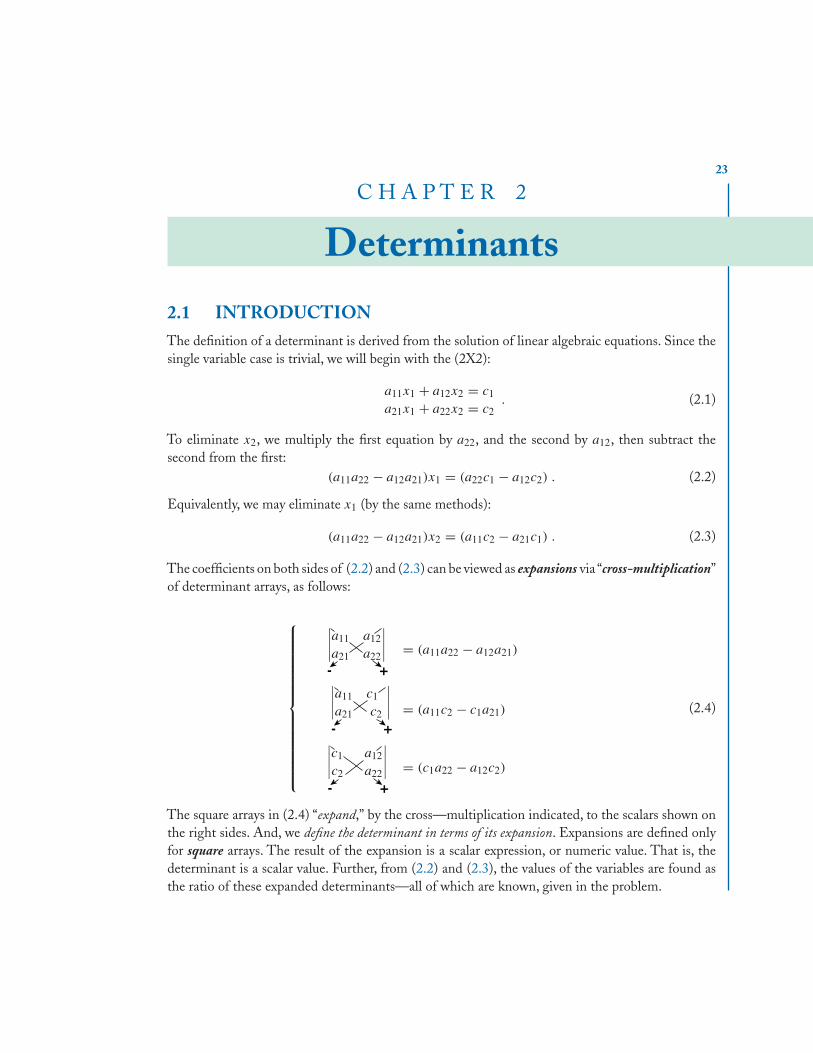
23
C H A P T E R 2
Determinants
2.1 INTRODUCTIONThe definition of a determinant is derived from the solution of linear algebraic equations. Since thesingle variable case is trivial, we will begin with the (2X2):
a11x1 + a12x2 = c1
a21x1 + a22x2 = c2. (2.1)
To eliminate x2, we multiply the first equation by a22, and the second by a12, then subtract thesecond from the first:
(a11a22 − a12a21)x1 = (a22c1 − a12c2) . (2.2)
Equivalently, we may eliminate x1 (by the same methods):
(a11a22 − a12a21)x2 = (a11c2 − a21c1) . (2.3)
The coefficients on both sides of (2.2) and (2.3) can be viewed as expansions via “cross-multiplication”of determinant arrays, as follows:
⎧⎪⎪⎪⎪⎪⎪⎪⎪⎪⎪⎪⎪⎪⎪⎨⎪⎪⎪⎪⎪⎪⎪⎪⎪⎪⎪⎪⎪⎪⎩
a11 a12a21 a22
+-= (a11a22 − a12a21)
a11 c1a21 c2
+-= (a11c2 − c1a21)
c1 a12c2 a22
+-= (c1a22 − a12c2)
(2.4)
The square arrays in (2.4) “expand,” by the cross—multiplication indicated, to the scalars shown onthe right sides. And, we define the determinant in terms of its expansion. Expansions are defined onlyfor square arrays. The result of the expansion is a scalar expression, or numeric value. That is, thedeterminant is a scalar value. Further, from (2.2) and (2.3), the values of the variables are found asthe ratio of these expanded determinants—all of which are known, given in the problem.
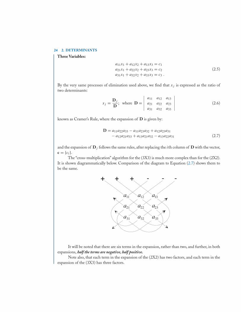
24 2. DETERMINANTS
Three Variables:
a11x1 + a12x2 + a13x3 = c1
a21x1 + a22x2 + a23x3 = c2
a31x1 + a32x2 + a33x3 = c3 .
(2.5)
By the very same processes of elimination used above, we find that xj is expressed as the ratio oftwo determinants:
xj = Dj
D; where D =
∣∣∣∣∣∣a11 a12 a13
a21 a22 a23
a31 a32 a33
∣∣∣∣∣∣ (2.6)
known as Cramer’s Rule, where the expansion of D is given by:
D = a11a22a33 − a11a23a32 + a12a23a31
− a12a21a33 + a13a21a32 − a13a22a31 (2.7)
and the expansion of Dj follows the same rules, after replacing the ith column of D with the vector,c = {ci}.
The “cross-multiplication” algorithm for the (3X3) is much more complex than for the (2X2).It is shown diagrammatically below. Comparison of the diagram to Equation (2.7) shows them tobe the same.
It will be noted that there are six terms in the expansion, rather than two, and further, in bothexpansions, half the terms are negative, half positive.
Note also, that each term in the expansion of the (2X2) has two factors, and each term in theexpansion of the (3X3) has three factors.
2.2. GENERAL DEFINITION OF A DETERMINANT 25
Now examine the row and column subscripts within each term: Every row (and column)subscript is represented once—and only once. This fact is extremely important to the developmentsthat follow.
Continuing with the expansions of the (4X4), then (5X5), and so on, it would be found thatthere are 24 terms in the expansion of the (4X4), and 120 terms in the (5X5) expansion. In thesecases, also, exactly half of the terms are positive, half negative. (Note: The statement that a term is“positive” or “negative” does not refer to the signs of the factors within the term. Half the terms inthe expansion of a determinant with all positive elements will be negative.) In these cases we wouldalso find that within every term, each row, and each column, subscript is represented exactly once.Then, each term in the expansion of a (4X4) has four factors, and each term in the expansion of the(5X5) contains five factors.
2.2 GENERAL DEFINITION OF A DETERMINANTThe general (nXn), determinant, |A|, can be represented as a square, two-dimensional array of ele-ments, each with two subscripts—the first indicating the element row position, the second indicatingcolumn position. Notwithstanding the two-dimensional representation, the determinant is a scalar.That is, it “expands” (as discussed above) to a scalar value—either a numeric, or a literal (function).
∣∣∣∣∣∣∣∣∣∣∣
a11 a12 a13 · · · a1n
a21 a22 a23 · · · a2n
a31 a32 a33 · · · a3n
· · · · · · · · · . . . · · ·an1 an2 an3 · · · ann
∣∣∣∣∣∣∣∣∣∣∣.
The expansion of |A| can be written as shown here:∣∣A∣∣ =∑
(−1)sa1ia2j a3k · · · (2.8)
Most of the remaining discussion in Sections 2.2 and 2.3 will refer to, and clarify, this equation.With respect to it, we note the following definitive statements:
1. The determinant, |A| expands into a sum of product terms.
2. Each term is the product of n elements from the array, where (nXn) is the dimension of thearray.
3. No two elements in any one term can come from the same row, or column. For example,Equation (2.8) implies that the elements were selected “in row order.” The first element fromrow 1 (any column, the ith), the second from row 2 (and any column except the ith), and soon. This process continues until all possible terms have been selected. As an example, everyterm in the expansion of a (4X4) will look like:
a1ia2j a3ka4l
26 2. DETERMINANTS
where i can be any one of 4 columns, j can be any one of three columns (but not the ith), k
can be one of two, and l must be the one remaining. In the (4X4) expansion, then, there willbe 4X3X2X1, or 24 terms.
4. In general, there will be n! terms in the expansion (2.8).
5. The sign to be affixed to each term will depend on the value of s, the superscript of the (−1)
factor, in (2.8). In every expansion, exactly half the terms will have a positive leading sign, halfa negative one.
The 5 statements given above define the general determinant, except for the term, (−1)s , in Equa-tion (2.8), whose value depends on whether the superscript, s, is odd or even.This will be the subjectof the next section.
Also, Equation (2.8) and its discussion imply that elements are to be selected “in row order”(the first element coming from the first row, etc.). But, of course, these factors could obviously bereordered within the terms. That is, they could have been chosen “in column order,” or indeed, inany order—just so long as no row or column index appears more than once in every term. But, it isimportant to note that every term in a determinant expansion can be arranged such that either rowor column index appears in numeric order. The other index will then be in some permutation of thisorder. Since there are n! permutations of n things, there are n! terms in the expansion.
2.3 PERMUTATIONS AND INVERSIONS OF INDICES
The subject of permutations is concerned with the arrangements of given things, or objects, in whichthe order of the arrangements is important. As an example, we ask: In how many ways can the digits1,2,3,4 be arranged into a four digit number? (Equivalently: How many permutations are there of 4things taken four at a time?). All the possible permutations of this example are:
1234 2134 3124 41231243 2143 3142 41321324 2314 3214 42131342 2341 3241 42311423 2413 3412 43121432 2431 3421 4321
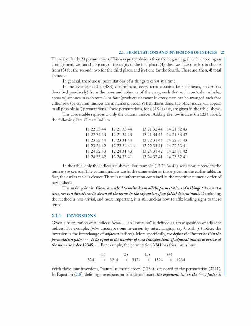
2.3. PERMUTATIONS AND INVERSIONS OF INDICES 27
There are clearly 24 permutations. This was pretty obvious from the beginning, since in choosing anarrangement, we can choose any of the digits in the first place, (4), then we have one less to choosefrom (3) for the second, two for the third place, and just one for the fourth. There are, then, 4! totalchoices.
In general, there are n! permutations of n things taken n at a time.In the expansion of a (4X4) determinant, every term contains four elements, chosen (as
described previously) from the rows and columns of the array, such that each row/column indexappears just once in each term. The four (product) elements in every term can be arranged such thateither row (or column) indices are in numeric order. When this is done, the other index will appearin all possible (n!) permutations. These permutations, for a (4X4) case, are given in the table, above.
The above table represents only the column indices. Adding the row indices (in 1234 order),the following lists all term indices.
11 22 33 44 12 21 33 44 13 21 32 44 14 21 32 4311 22 34 43 12 21 34 43 13 21 34 42 14 21 33 4211 23 32 44 12 23 31 44 13 22 31 44 14 22 31 4311 23 34 42 12 23 34 41 ← 13 22 34 41 14 22 33 4111 24 32 43 12 24 31 43 13 24 31 42 14 23 31 4211 24 33 42 12 24 33 41 13 24 32 41 14 23 32 41
In the table, only the indices are shown. For example, (12 23 34 41), see arrow, represents theterm a12a23a34a41. The column indices are in the same order as those given in the earlier table. Infact, the earlier table is clearer. There is no information contained in the repetitive numeric order ofrow indices.
The main point is: Given a method to write down all the permutations of n things taken n at atime, we can directly write down all the terms in the expansion of an (nXn) determinant . Developingthe method is non-trivial, and more important, it is still unclear how to affix leading signs to theseterms.
2.3.1 INVERSIONSGiven a permutation of n indices: ijklm· · ·, an “inversion” is defined as a transposition of adjacentindices. For example, ijklm undergoes one inversion by interchanging, say k with j (notice: theinversion is the interchange of adjacent indices). More specifically, we define the “inversions” in thepermutation ijklm· · ··, to be equal to the number of such transpositions of adjacent indices to arrive atthe numeric order 12345· · ·. For example, the permutation 3241 has four inversions:
(1) (2) (3) (4)
3241 → 3214 → 3124 → 1324 → 1234
With these four inversions, “natural numeric order” (1234) is restored to the permutation (3241).In Equation (2.8), defining the expansion of a determinant, the exponent, “s,” on the (−1) factor is
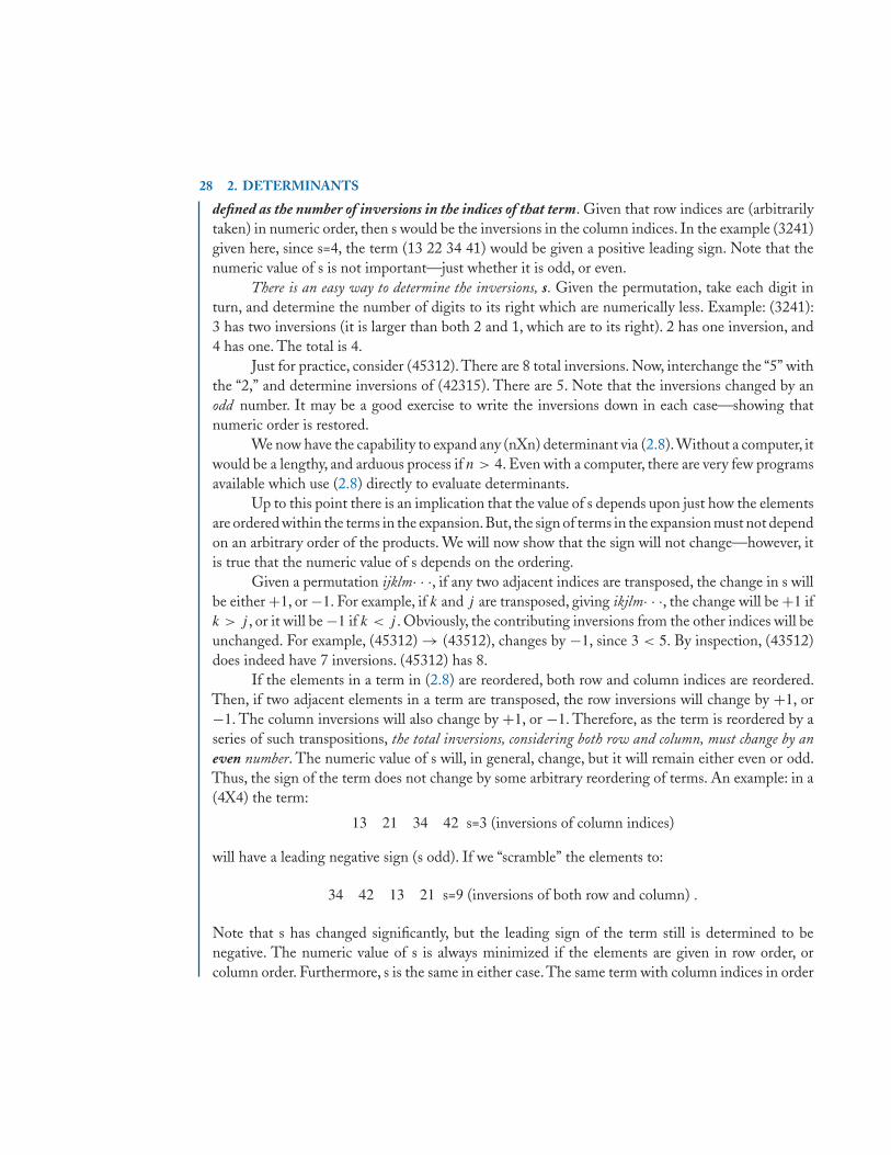
28 2. DETERMINANTS
defined as the number of inversions in the indices of that term. Given that row indices are (arbitrarilytaken) in numeric order, then s would be the inversions in the column indices. In the example (3241)given here, since s=4, the term (13 22 34 41) would be given a positive leading sign. Note that thenumeric value of s is not important—just whether it is odd, or even.
There is an easy way to determine the inversions, s. Given the permutation, take each digit inturn, and determine the number of digits to its right which are numerically less. Example: (3241):3 has two inversions (it is larger than both 2 and 1, which are to its right). 2 has one inversion, and4 has one. The total is 4.
Just for practice, consider (45312).There are 8 total inversions. Now, interchange the “5” withthe “2,” and determine inversions of (42315). There are 5. Note that the inversions changed by anodd number. It may be a good exercise to write the inversions down in each case—showing thatnumeric order is restored.
We now have the capability to expand any (nXn) determinant via (2.8).Without a computer, itwould be a lengthy, and arduous process if n > 4. Even with a computer, there are very few programsavailable which use (2.8) directly to evaluate determinants.
Up to this point there is an implication that the value of s depends upon just how the elementsare ordered within the terms in the expansion.But, the sign of terms in the expansion must not dependon an arbitrary order of the products. We will now show that the sign will not change—however, itis true that the numeric value of s depends on the ordering.
Given a permutation ijklm· · ·, if any two adjacent indices are transposed, the change in s willbe either +1, or −1. For example, if k and j are transposed, giving ikjlm· · ·, the change will be +1 ifk > j , or it will be −1 if k < j . Obviously, the contributing inversions from the other indices will beunchanged. For example, (45312) → (43512), changes by −1, since 3 < 5. By inspection, (43512)does indeed have 7 inversions. (45312) has 8.
If the elements in a term in (2.8) are reordered, both row and column indices are reordered.Then, if two adjacent elements in a term are transposed, the row inversions will change by +1, or−1. The column inversions will also change by +1, or −1. Therefore, as the term is reordered by aseries of such transpositions, the total inversions, considering both row and column, must change by aneven number. The numeric value of s will, in general, change, but it will remain either even or odd.Thus, the sign of the term does not change by some arbitrary reordering of terms. An example: in a(4X4) the term:
13 21 34 42 s=3 (inversions of column indices)
will have a leading negative sign (s odd). If we “scramble” the elements to:
34 42 13 21 s=9 (inversions of both row and column) .
Note that s has changed significantly, but the leading sign of the term still is determined to benegative. The numeric value of s is always minimized if the elements are given in row order, orcolumn order. Furthermore, s is the same in either case.The same term with column indices in order
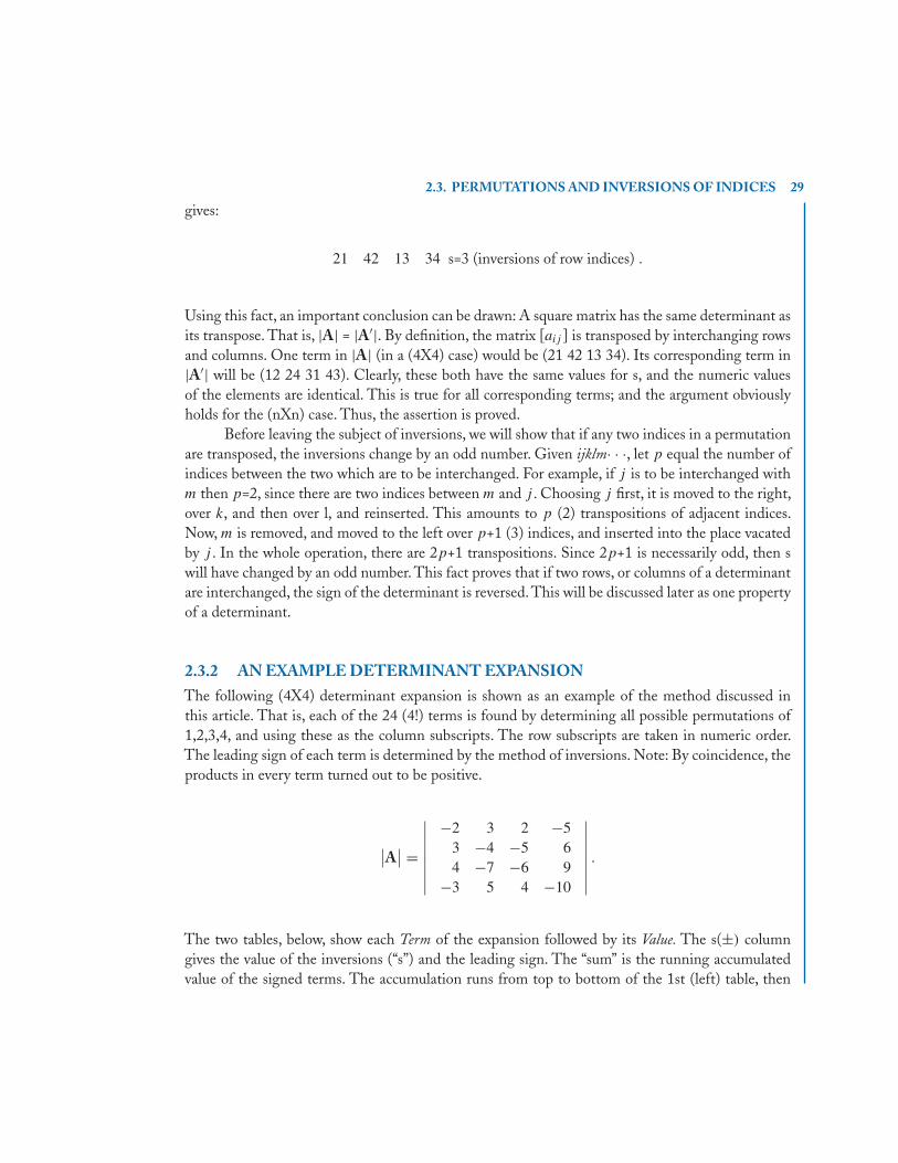
2.3. PERMUTATIONS AND INVERSIONS OF INDICES 29
gives:
21 42 13 34 s=3 (inversions of row indices) .
Using this fact, an important conclusion can be drawn: A square matrix has the same determinant asits transpose. That is, |A| = |A′|. By definition, the matrix [aij ] is transposed by interchanging rowsand columns. One term in |A| (in a (4X4) case) would be (21 42 13 34). Its corresponding term in|A′| will be (12 24 31 43). Clearly, these both have the same values for s, and the numeric valuesof the elements are identical. This is true for all corresponding terms; and the argument obviouslyholds for the (nXn) case. Thus, the assertion is proved.
Before leaving the subject of inversions, we will show that if any two indices in a permutationare transposed, the inversions change by an odd number. Given ijklm· · ·, let p equal the number ofindices between the two which are to be interchanged. For example, if j is to be interchanged withm then p=2, since there are two indices between m and j . Choosing j first, it is moved to the right,over k, and then over l, and reinserted. This amounts to p (2) transpositions of adjacent indices.Now, m is removed, and moved to the left over p+1 (3) indices, and inserted into the place vacatedby j . In the whole operation, there are 2p+1 transpositions. Since 2p+1 is necessarily odd, then swill have changed by an odd number. This fact proves that if two rows, or columns of a determinantare interchanged, the sign of the determinant is reversed. This will be discussed later as one propertyof a determinant.
2.3.2 AN EXAMPLE DETERMINANT EXPANSIONThe following (4X4) determinant expansion is shown as an example of the method discussed inthis article. That is, each of the 24 (4!) terms is found by determining all possible permutations of1,2,3,4, and using these as the column subscripts. The row subscripts are taken in numeric order.The leading sign of each term is determined by the method of inversions. Note: By coincidence, theproducts in every term turned out to be positive.
∣∣A∣∣ =
∣∣∣∣∣∣∣∣−2 3 2 −5
3 −4 −5 64 −7 −6 9
−3 5 4 −10
∣∣∣∣∣∣∣∣.
The two tables, below, show each Term of the expansion followed by its Value. The s(±) columngives the value of the inversions (“s”) and the leading sign. The “sum” is the running accumulatedvalue of the signed terms. The accumulation runs from top to bottom of the 1st (left) table, then
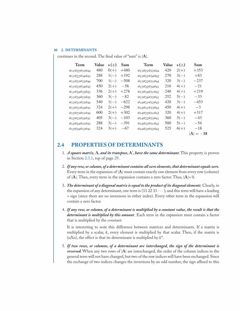
30 2. DETERMINANTS
continues in the second. The final value of “sum” is |A|.Term Value s (±) Sum Term Value s (±) Sum
a11a22a33a44 480 0(+) +480 a13a21a32a44 420 2(+) +353a11a22a34a43 288 1(−) +192 a13a21a34a42 270 3(−) +83a11a23a32a44 700 1(−) −508 a13a22a31a44 320 3(−) −237a11a23a34a42 450 2(+) −58 a13a22a34a41 216 4(+) −21a11a24a32a43 336 2(+) +278 a13a24a31a42 240 4(+) +219a11a24a33a42 360 3(−) −82 a13a24a32a41 252 5(−) −33a12a21a33a44 540 1(−) −622 a14a21a32a43 420 3(−) −453a12a21a34a43 324 2(+) −298 a14a21a33a42 450 4(+) −3a12a23a31a44 600 2(+) +302 a14a22a31a43 320 4(+) +317a12a23a34a41 405 3(−) −103 a14a22a33a41 360 5(−) −43a12a24a31a43 288 3(−) −391 a14a23a31a42 500 5(−) −54a12a24a33a41 324 3(+) −67 a14a23a32a41 525 6(+) −18
|A| = - 18
2.4 PROPERTIES OF DETERMINANTS1. A square matrix, A, and its transpose, A′, have the same determinant. This property is proven
in Section 2.3.1, top of page 29.
2. If any row, or column, of a determinant contains all zero elements, that determinant equals zero.Every term in the expansion of |A| must contain exactly one element from every row (column)of |A|. Then, every term in the expansion contains a zero factor. Thus, |A|= 0.
3. The determinant of a diagonal matrix is equal to the product of its diagonal elements. Clearly, inthe expansion of any determinant, one term is (11 22 33 · · · ); and this term will have a leading+ sign (since there are no inversions in either index). Every other term in the expansion willcontain a zero factor.
4. If any row, or column, of a determinant is multiplied by a constant value, the result is that thedeterminant is multiplied by this amount . Each term in the expansion must contain a factorthat is multiplied by the constant.
It is interesting to note this difference between matrices and determinants. If a matrix ismultiplied by a scalar, k, every element is multiplied by that scalar. Then, if the matrix is(nXn), the effect is that its determinant is multiplied by kn.
5. If two rows, or columns, of a determinant are interchanged, the sign of the determinant isreversed. When any two rows of |A| are interchanged, the order of the column indices in thegeneral term will not have changed, but two of the row indices will have been exchanged. Sincethe exchange of two indices changes the inversions by an odd number, the sign affixed to this
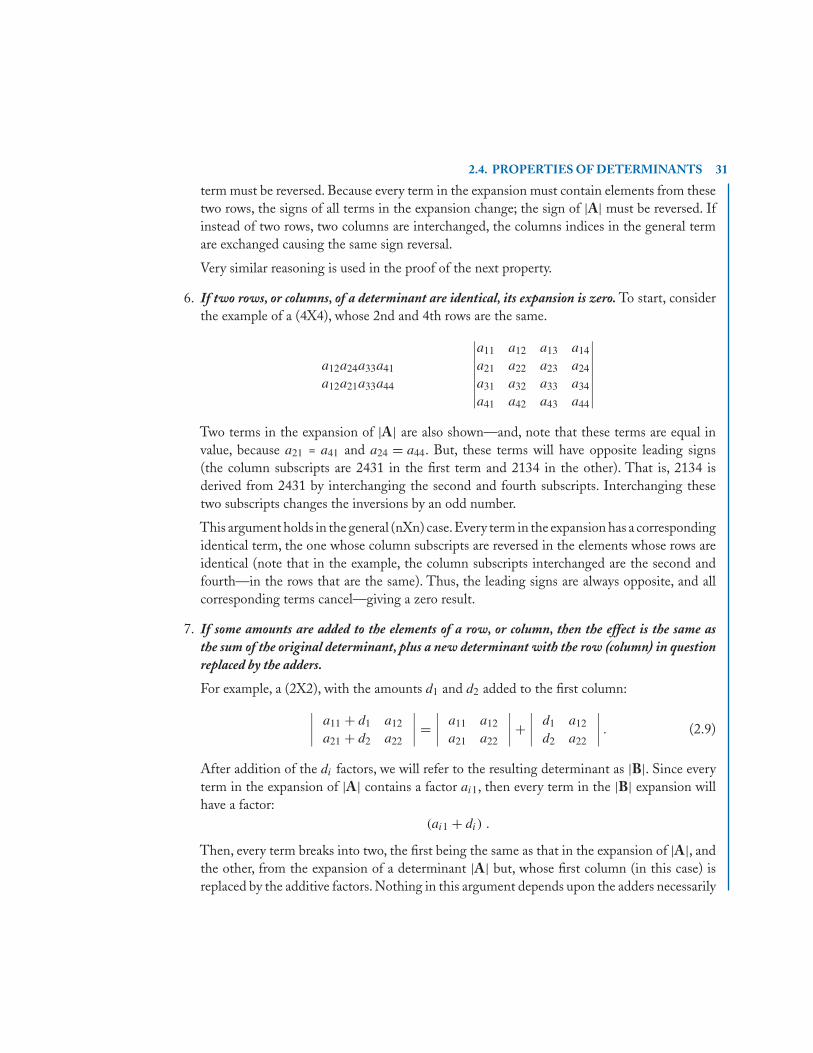
2.4. PROPERTIES OF DETERMINANTS 31
term must be reversed. Because every term in the expansion must contain elements from thesetwo rows, the signs of all terms in the expansion change; the sign of |A| must be reversed. Ifinstead of two rows, two columns are interchanged, the columns indices in the general termare exchanged causing the same sign reversal.
Very similar reasoning is used in the proof of the next property.
6. If two rows, or columns, of a determinant are identical, its expansion is zero. To start, considerthe example of a (4X4), whose 2nd and 4th rows are the same.
a12a24a33a41
a12a21a33a44
∣∣∣∣∣∣∣∣a11 a12 a13 a14
a21 a22 a23 a24
a31 a32 a33 a34
a41 a42 a43 a44
∣∣∣∣∣∣∣∣Two terms in the expansion of |A| are also shown—and, note that these terms are equal invalue, because a21 = a41 and a24 = a44. But, these terms will have opposite leading signs(the column subscripts are 2431 in the first term and 2134 in the other). That is, 2134 isderived from 2431 by interchanging the second and fourth subscripts. Interchanging thesetwo subscripts changes the inversions by an odd number.
This argument holds in the general (nXn) case.Every term in the expansion has a correspondingidentical term, the one whose column subscripts are reversed in the elements whose rows areidentical (note that in the example, the column subscripts interchanged are the second andfourth—in the rows that are the same). Thus, the leading signs are always opposite, and allcorresponding terms cancel—giving a zero result.
7. If some amounts are added to the elements of a row, or column, then the effect is the same asthe sum of the original determinant, plus a new determinant with the row (column) in questionreplaced by the adders.
For example, a (2X2), with the amounts d1 and d2 added to the first column:∣∣∣∣ a11 + d1 a12
a21 + d2 a22
∣∣∣∣ =∣∣∣∣ a11 a12
a21 a22
∣∣∣∣+∣∣∣∣ d1 a12
d2 a22
∣∣∣∣ . (2.9)
After addition of the di factors, we will refer to the resulting determinant as |B|. Since everyterm in the expansion of |A| contains a factor ai1, then every term in the |B| expansion willhave a factor:
(ai1 + di) .
Then, every term breaks into two, the first being the same as that in the expansion of |A|, andthe other, from the expansion of a determinant |A| but, whose first column (in this case) isreplaced by the additive factors. Nothing in this argument depends upon the adders necessarily
32 2. DETERMINANTS
being added to the first column. And the argument holds if the adders are on a row ratherthan a column.
Now, if the di adders happen to be a constant, k, times the elements of some other column,then (after factoring the k) the second determinant in (2.9) is one in which two rows areidentical. In that case, the second determinant is zero, by property 6. Then:
8. If to any row, or column, there is added a constant factor multiplied by the corresponding elementsof any other row, or column, the value of the determinant is unchanged . This is an extremelyimportant property. It is almost always utilized in the expansion of determinants.
It is important to generalize property 2. Consider an (nXn) determinant, |A|, one of whoserows (or columns), say the j th, is initially zero—i.e., all the j th elements are zero. Then, byproperty 2, |A|=0. Now, by repetitive use of property 8, add to the j th (row/column) arbitrarymultiples of other rows (columns). The result is (assuming a row):
rowj = c1(row 1) + c2(row 2) + · · · + cn(row n) (2.10)
where the row-sums in (2.10) are to be viewed as element-by-element additions. For example,“row1+row2” would be viewed just like two vectors would be added:
|(a11 + a21)(a12 + a22) · · · (a1n + a2n)| .
Also in (2.10), some, but not all, of the ck values could be zero.
Now, the j th row (originally all zero), is no longer zero, and its elements are not equal tothose of any other single row. Yet, property 8 insists that the value of the determinant has notchanged by these additions (or subtractions; note that some, or all of the ck could be negative).Then, the value of |A| must still be zero. We, therefore, conclude the property:
9. If any row, or column, of a determinant is a “linear combination” of the other rows, or columns,then that determinant is zero. By definition, the “linear combination” is the summation givenin (2.10).
The reader may remember this property from the algebraic solution to sets of linear equations. Inorder to achieve a unique solution of n equations in n unknowns,n independent equations are needed.If one (or more) of these equations is a “linear combination” of the others, then a unique solutiondoes not exist. This will be a subject in a later chapter.
2.5 THE RANK OF A DETERMINANTContinuing the discussion of the last article, consider an (nXn) determinant whose value is zero byvirtue of property 9. If just one of its rows (or columns) is a linear combination of the others, then its“rank” is said to be (n − 1). If two rows (or columns) are linear combinations of the others, then itsrank is (n − 2). And so on. On the other hand, if all n of the rows (or columns) of |A| are “linearly
2.6. MINORS AND COFACTORS 33
independent” (i.e., none of the rows (columns) is a linear combination of the others), then the rankof |A| is n (and its determinant is nonzero).
A more accurate way to say the above is: If the rows (columns) of a determinant are linearcombinations of (n − k) independent rows (columns), then the rank of the determinant is (n − k).
In summary, an (nXn) determinant (or square matrix) may have a maximum rank of n, if thedeterminant does not vanish (not zero). Its minimum rank would be zero, if all its elements are zero(a trivial case).
If |A| is not zero, its rank is n. If its rank is (n − 1) then there exists at least one (n−1Xn−1)determinant made up of the rows (columns) of |A| that is not zero. If its rank is (n − 2), then at leastone (n−2Xn−2) non-zero determinant can be found. And so on. The subject of “rank of a matrix”will come up in a future chapter.
2.6 MINORS AND COFACTORSIf one, or more, rows and columns are deleted from a determinant, the result is a determinant oflower order, and is called a “minor” of the original. If just one row and one column are deleted, theresulting “first minor” is of order (n − 1). Clearly, within an |nXn|, there exist n2 first minors. The“second minor” is of order (n − 2), and is the result of deleting 2 rows and 2 columns. In this sameway, minors of various orders can be defined. A minor is a determinant, and must, therefore, alwayshave the same number of rows as columns.
The elements which lie at the intersections of the deleted rows and columns also form adeterminant, which is called the “complement” of the minor. Note that the complement of a firstminor is a single 1X1 element.
Of particular interest are the first minors.These are of order n − 1, and result from the deletionof the ith row, and j th column. The complement is the element aij , and the minor will be denotedMij .
2.6.1 EXPANSIONS BY MINORS—LAPLACE EXPANSIONSThe LaPlace expansion is defined as follows. Select any number, say r , rows (or columns) from |A|.Then, the value of |A| is equal to the sum of products of all the rth order minors contained in theser rows (columns) each multiplied by its corresponding algebraic complement (the complement withthe correct leading sign attached). Of greatest importance are the first minors.
Expansion by First MinorsThe table below has been taken from Section 2.3. It lists all the indices in the expansion of a (4X4).In this table, leading signs have been added, according to the inversions rules already discussed.
Inspection of the first column in Table 2.1 shows that, when a11 is factored, the terms repre-sented in this column can be written:
a11(a22a33a44 − a22a34a43 − a23a32a44 + a23a34a42 + a24a32a42 − a24a33a42)
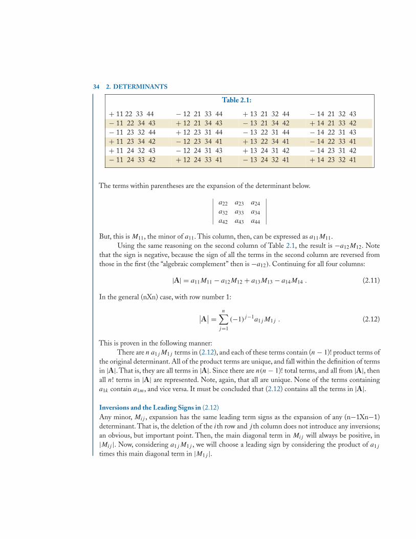
34 2. DETERMINANTS
Table 2.1:
+ 11 22 33 44 − 12 21 33 44 + 13 21 32 44 − 14 21 32 43− 11 22 34 43 + 12 21 34 43 − 13 21 34 42 + 14 21 33 42− 11 23 32 44 + 12 23 31 44 − 13 22 31 44 − 14 22 31 43+ 11 23 34 42 − 12 23 34 41 + 13 22 34 41 − 14 22 33 41+ 11 24 32 43 − 12 24 31 43 + 13 24 31 42 − 14 23 31 42− 11 24 33 42 + 12 24 33 41 − 13 24 32 41 + 14 23 32 41
The terms within parentheses are the expansion of the determinant below.
∣∣∣∣∣∣a22 a23 a24
a32 a33 a34
a42 a43 a44
∣∣∣∣∣∣But, this is M11, the minor of a11. This column, then, can be expressed as a11M11.
Using the same reasoning on the second column of Table 2.1, the result is −a12M12. Notethat the sign is negative, because the sign of all the terms in the second column are reversed fromthose in the first (the “algebraic complement” then is −a12). Continuing for all four columns:
|A| = a11M11 − a12M12 + a13M13 − a14M14 . (2.11)
In the general (nXn) case, with row number 1:
∣∣A∣∣ =n∑
j=1
(−1)j−1a1jM1j . (2.12)
This is proven in the following manner:There are n a1jM1j terms in (2.12), and each of these terms contain (n − 1)! product terms of
the original determinant. All of the product terms are unique, and fall within the definition of termsin |A|. That is, they are all terms in |A|. Since there are n(n − 1)! total terms, and all from |A|, thenall n! terms in |A| are represented. Note, again, that all are unique. None of the terms containinga1k contain a1m, and vice versa. It must be concluded that (2.12) contains all the terms in |A|.
Inversions and the Leading Signs in (2.12)Any minor, Mij , expansion has the same leading term signs as the expansion of any (n−1Xn−1)determinant. That is, the deletion of the ith row and j th column does not introduce any inversions;an obvious, but important point. Then, the main diagonal term in Mij will always be positive, in|Mij |. Now, considering a1jM1j , we will choose a leading sign by considering the product of a1j
times this main diagonal term in |M1j |.
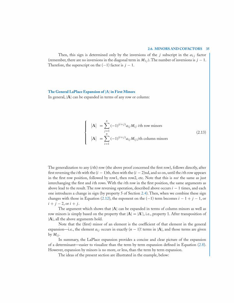
2.6. MINORS AND COFACTORS 35
Then, this sign is determined only by the inversions of the j subscript in the a1j factor(remember, there are no inversions in the diagonal term in M1j ). The number of inversions is j − 1.Therefore, the superscript on the (−1) factor is j − 1.
The General LaPlace Expansion of |A| in First MinorsIn general, |A| can be expanded in terms of any row or column:
⎧⎪⎪⎪⎪⎨⎪⎪⎪⎪⎩
∣∣A∣∣ =n∑
j=1
(−1)(i+j)aijMij ith row minors
∣∣A∣∣ =n∑
i=1
(−1)(i+j)aijMij j th column minors
(2.13)
The generalization to any (ith) row (the above proof concerned the first row), follows directly, afterfirst reversing the ith with the (i − 1)th, then with the (i − 2)nd, and so on, until the ith row appearsin the first row position, followed by row1, then row2, etc. Note that this is not the same as justinterchanging the first and ith rows. With the ith row in the first position, the same arguments asabove lead to the result. The row reversing operation, described above occurs i − 1 times, and eachone introduces a change in sign (by property 5 of Section 2.4). Then, when we combine these signchanges with those in Equation (2.12), the exponent on the (−1) term becomes i − 1 + j − 1, ori + j − 2, or i + j .
The argument which shows that |A| can be expanded in terms of column minors as well asrow minors is simply based on the property that |A| = |A′|, i.e., property 1. After transposition of|A|, all the above arguments hold.
Note that the (first) minor of an element is the coefficient of that element in the generalexpansion—i.e., the element aij occurs in exactly (n − 1)! terms in |A|, and those terms are givenby Mij .
In summary, the LaPlace expansion provides a concise and clear picture of the expansionof a determinant—easier to visualize than the term by term expansion defined in Equation (2.8).However, expansion by minors is no more, or less, than the term by term expansion.
The ideas of the present section are illustrated in the example, below:
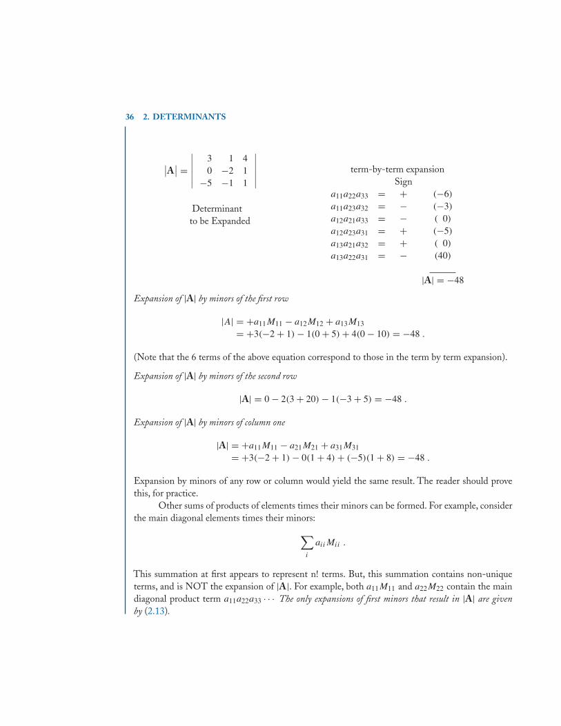
36 2. DETERMINANTS
∣∣A∣∣ =∣∣∣∣∣∣
3 1 40 −2 1
−5 −1 1
∣∣∣∣∣∣Determinant
to be Expanded
term-by-term expansionSign
a11a22a33 = + (−6)
a11a23a32 = − (−3)
a12a21a33 = − ( 0)
a12a23a31 = + (−5)
a13a21a32 = + ( 0)
a13a22a31 = − (40)
|A| = −48
Expansion of |A| by minors of the first row
|A| = +a11M11 − a12M12 + a13M13
= +3(−2 + 1) − 1(0 + 5) + 4(0 − 10) = −48 .
(Note that the 6 terms of the above equation correspond to those in the term by term expansion).
Expansion of |A| by minors of the second row
|A| = 0 − 2(3 + 20) − 1(−3 + 5) = −48 .
Expansion of |A| by minors of column one
|A| = +a11M11 − a21M21 + a31M31
= +3(−2 + 1) − 0(1 + 4) + (−5)(1 + 8) = −48 .
Expansion by minors of any row or column would yield the same result. The reader should provethis, for practice.
Other sums of products of elements times their minors can be formed. For example, considerthe main diagonal elements times their minors:
∑i
aiiMii .
This summation at first appears to represent n! terms. But, this summation contains non-uniqueterms, and is NOT the expansion of |A|. For example, both a11M11 and a22M22 contain the maindiagonal product term a11a22a33 · · · The only expansions of first minors that result in |A| are givenby (2.13).
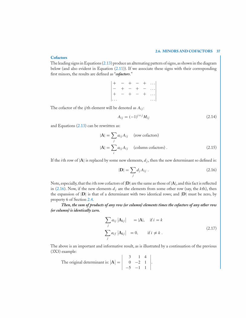
2.6. MINORS AND COFACTORS 37
CofactorsThe leading signs in Equations (2.13) produce an alternating pattern of signs,as shown in the diagrambelow (and also evident in Equation (2.11)). If we associate these signs with their correspondingfirst minors, the results are defined as “cofactors.”∣∣∣∣∣∣∣∣
+ − + − + . . .
− + − + − . . .
+ − + − + . . .
. . . . . .
∣∣∣∣∣∣∣∣The cofactor of the ijth element will be denoted as Aij :
Aij = (−1)i+jMij (2.14)
and Equations (2.13) can be rewritten as:
|A| =∑j
aijAij (row cofactors)
|A| =∑
i
aijAij (column cofactors) . (2.15)
If the ith row of |A| is replaced by some new elements, dj , then the new determinant so defined is:
|D| =∑j
djAij . (2.16)
Note, especially, that the ith row cofactors of |D| are the same as those of |A|, and this fact is reflectedin (2.16). Now, if the new elements dj are the elements from some other row (say, the kth), thenthe expansion of |D| is that of a determinant with two identical rows; and |D| must be zero, byproperty 6 of Section 2.4.
Then, the sum of products of any row (or column) elements times the cofactors of any other row(or column) is identically zero. ∑
j
aij
∣∣Akj
∣∣ = |A|, if i = k
∑j
aif
∣∣Akj
∣∣ = 0, if i �= k .(2.17)
The above is an important and informative result, as is illustrated by a continuation of the previous(3X3) example:
The original determinant is:∣∣A∣∣ =
∣∣∣∣∣∣3 1 40 −2 1
−5 −1 1
∣∣∣∣∣∣.
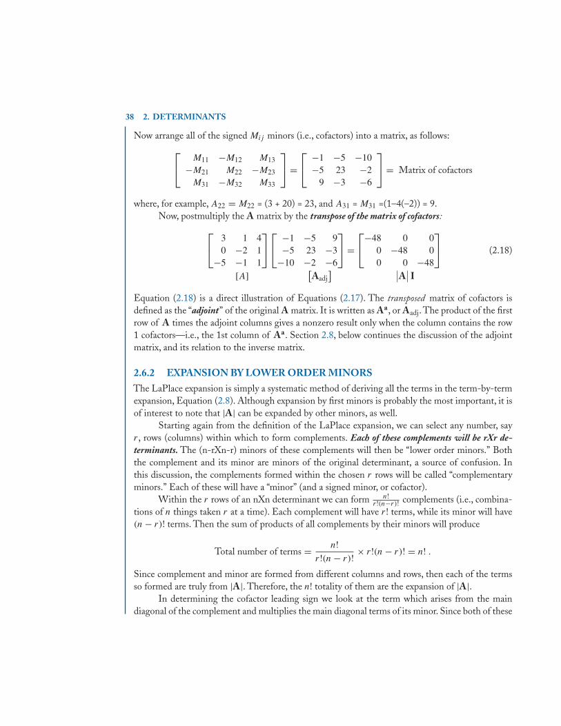
38 2. DETERMINANTS
Now arrange all of the signed Mij minors (i.e., cofactors) into a matrix, as follows:
⎡⎣ M11 −M12 M13
−M21 M22 −M23
M31 −M32 M33
⎤⎦ =
⎡⎣ −1 −5 −10
−5 23 −29 −3 −6
⎤⎦ = Matrix of cofactors
where, for example, A22 = M22 = (3 + 20) = 23, and A31 = M31 =(1–4(–2)) = 9.Now, postmultiply the A matrix by the transpose of the matrix of cofactors:
⎡⎣ 3 1 4
0 −2 1−5 −1 1
⎤⎦⎡⎣ −1 −5 9
−5 23 −3−10 −2 −6
⎤⎦ =
⎡⎣−48 0 0
0 −48 00 0 −48
⎤⎦ (2.18)
[A][Aadj
] ∣∣A∣∣ I
Equation (2.18) is a direct illustration of Equations (2.17). The transposed matrix of cofactors isdefined as the “adjoint” of the original A matrix. It is written as Aa , or Aadj. The product of the firstrow of A times the adjoint columns gives a nonzero result only when the column contains the row1 cofactors—i.e., the 1st column of Aa . Section 2.8, below continues the discussion of the adjointmatrix, and its relation to the inverse matrix.
2.6.2 EXPANSION BY LOWER ORDER MINORSThe LaPlace expansion is simply a systematic method of deriving all the terms in the term-by-termexpansion, Equation (2.8). Although expansion by first minors is probably the most important, it isof interest to note that |A| can be expanded by other minors, as well.
Starting again from the definition of the LaPlace expansion, we can select any number, sayr , rows (columns) within which to form complements. Each of these complements will be rXr de-terminants. The (n-rXn-r) minors of these complements will then be “lower order minors.” Boththe complement and its minor are minors of the original determinant, a source of confusion. Inthis discussion, the complements formed within the chosen r rows will be called “complementaryminors.” Each of these will have a “minor” (and a signed minor, or cofactor).
Within the r rows of an nXn determinant we can form n!r!(n−r)! complements (i.e., combina-
tions of n things taken r at a time). Each complement will have r ! terms, while its minor will have(n − r)! terms. Then the sum of products of all complements by their minors will produce
Total number of terms = n!r!(n − r)! × r!(n − r)! = n! .
Since complement and minor are formed from different columns and rows, then each of the termsso formed are truly from |A|. Therefore, the n! totality of them are the expansion of |A|.
In determining the cofactor leading sign we look at the term which arises from the maindiagonal of the complement and multiplies the main diagonal terms of its minor. Since both of these
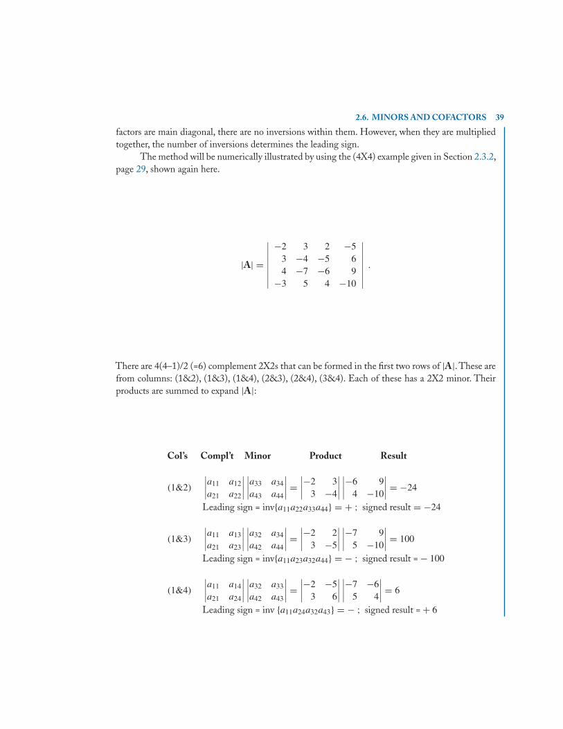
2.6. MINORS AND COFACTORS 39
factors are main diagonal, there are no inversions within them. However, when they are multipliedtogether, the number of inversions determines the leading sign.
The method will be numerically illustrated by using the (4X4) example given in Section 2.3.2,page 29, shown again here.
|A| =
∣∣∣∣∣∣∣∣−2 3 2 −5
3 −4 −5 64 −7 −6 9
−3 5 4 −10
∣∣∣∣∣∣∣∣.
There are 4(4–1)/2 (=6) complement 2X2s that can be formed in the first two rows of |A|. These arefrom columns: (1&2), (1&3), (1&4), (2&3), (2&4), (3&4). Each of these has a 2X2 minor. Theirproducts are summed to expand |A|:
Col’s Compl’t Minor Product Result
(1&2)
∣∣∣∣a11 a12
a21 a22
∣∣∣∣∣∣∣∣a33 a34
a43 a44
∣∣∣∣ =∣∣∣∣−2 3
3 −4
∣∣∣∣∣∣∣∣−6 9
4 −10
∣∣∣∣ = −24
Leading sign = inv{a11a22a33a44} = + ; signed result = −24
(1&3)
∣∣∣∣a11 a13
a21 a23
∣∣∣∣∣∣∣∣a32 a34
a42 a44
∣∣∣∣ =∣∣∣∣−2 2
3 −5
∣∣∣∣∣∣∣∣−7 9
5 −10
∣∣∣∣ = 100
Leading sign = inv{a11a23a32a44} = − ; signed result = − 100
(1&4)
∣∣∣∣a11 a14
a21 a24
∣∣∣∣∣∣∣∣a32 a33
a42 a43
∣∣∣∣ =∣∣∣∣−2 −5
3 6
∣∣∣∣∣∣∣∣−7 −6
5 4
∣∣∣∣ = 6
Leading sign = inv {a11a24a32a43} = − ; signed result = + 6

40 2. DETERMINANTS
Col’s Compl’t Minor Product Result
(2&3)
∣∣∣∣a12 a13
a22 a23
∣∣∣∣∣∣∣∣a31 a34
a41 a44
∣∣∣∣ =∣∣∣∣ 3 2−4 −5
∣∣∣∣∣∣∣∣ 4 9−3 −10
∣∣∣∣ = 91
Leading sign = inv{a12a23a31a44} = + ; signed result = + 91
(2&4)
∣∣∣∣a12 a14
a22 a24
∣∣∣∣∣∣∣∣a31 a33
a41 a43
∣∣∣∣ =∣∣∣∣ 3 −5−4 6
∣∣∣∣∣∣∣∣ 4 −6−3 4
∣∣∣∣ = 4
Leading sign = inv{a12a24a31a43} = − ; signed result = − 4
(3&4)
∣∣∣∣a13 a14
a23 a24
∣∣∣∣∣∣∣∣a31 a32
a41 a42
∣∣∣∣ =∣∣∣∣−2 −5−5 6
∣∣∣∣∣∣∣∣ 4 −7−3 5
∣∣∣∣ = 13
Leading sign = inv{a13a24a31a42} = + ; signed result = + 13 .
Adding the signed results, above, yields the value of |A| = −18, (the same as in Section 2.3.2).If |A| were (7X7), and its first 3 rows are chosen in which to form the complements (which
will be 3X3’s), the number of complements will be equal to 35, the number of combinations of 7things taken 3 at a time:
Number of complements = n!r!(n − r)! = 7!
3!4! = 7 • 6 • 5
3 • 2= 35 .
Each of the 3X3 complements will have a 4X4 cofactor, formed within the lower 4 rows, and usingthe 4 columns that are not used in the complement. Each complement expands to 3! = 6 terms, andits cofactor has 4! = 24 terms. Then the total number of terms will be 35•6•24 = 7!. This is thecorrect number of terms needed in the expansion of a 7X7, and note that every term is taken fromelements of separate rows and columns, as required.
In determining the cofactor leading sign we look at the term which arises from the maindiagonal of the 3X3 and multiplies the main diagonal terms of its minor. For example, one of thecomplements will be formed using the first 3 rows and columns 1, 4, and 6. Its main diagonal termis
a11a24a36 and the cofactor main diagonal is a42a53a65a77 .
Of course, there are no inversions within these. However, when these terms are multiplied:
a11a24a36a42a53a65a77 ⇒ Inversions in 1462357 = 5 (odd) .
Therefore, the leading sign of the product of this complement times its minor must be negative.

2.7. GEOMETRY: LINES, AREAS, AND VOLUMES 41
2.6.3 THE DETERMINANT OF A MATRIX PRODUCTThe LaPlace expansion methods are not convenient for use in expanding determinants, but theygive valuable insight into the problem. For example, consider:
C =[
0 X−I B
]where C = (2nX2n) and the partitioned matrices are (nXn) .
To find |C|, expansion by complements in the first n rows is the obvious choice—there will only beone such complement since all others will have a zero column. The complement will be |X|, but itmight appear that the negative sign on I may alter the sign of the result depending upon n-odd oreven. But, look at the inversions in the column indices. They will be:
[(n + 1)(n + 2) · · · (2n)][(1 · 2 · 3·, , ·n)] Example: If n = 2: column indices are 3412 .
Clearly, there will always be n2 inversions. How nice. Whenever n is odd, the leading sign is negative,just “canceling” the negative value of |–I|. Thus, |C| = |X| for any n.
This result is prominent in the proof that the determinant of a matrix product is the productof their determinants. Consider the matrix equation
C =[
I A0 I
] [A 0
−I B
]=[
0 AB−I B
]. (2.19)
Since the matrices on each side of the equality are identical, they must have the same determinant.So, we may “take determinants of both sides.” In so doing, note that the first matrix on the left is a“Fundamental Operations” matrix which causes sums and/or differences of rows to be combined withthe original rows in the second matrix. These operations do not affect the value of the determinant(Property 8). So:
|C| =∣∣∣∣ A 0
−I B
∣∣∣∣ =∣∣∣∣ 0 AB
−I B
∣∣∣∣ . (2.20)
The determinant on the left, expanded by minors of the first n rows, is clearly equal to |A||B|. Thedeterminant on the right has just been shown to be |AB|. Then:
|C| = ∣∣A∣∣ |B| = ∣∣AB∣∣ . (2.21)
The extension of this to multiple matrices in the product is obvious.
2.7 GEOMETRY: LINES, AREAS, AND VOLUMESThe “Two-point form” of the equation of a line can be written as the following determinant∣∣∣∣∣∣
x y 1x1 y1 1x2 y2 1
∣∣∣∣∣∣ = 0 ⇒ y = y2 − y1
x2 − x1x + y1x2 − y2x1
x2 − x1. (2.22)
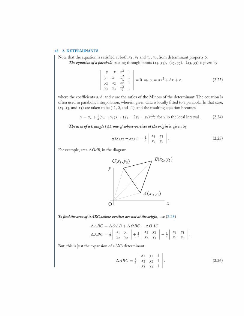
42 2. DETERMINANTS
Note that the equation is satisfied at both x1, y1 and x2, y2, from determinant property 6.The equation of a parabola passing through points (x1, y1), (x2, y2), (x3, y3) is given by
∣∣∣∣∣∣∣∣y x x2 1
y1 x1 x21 1
y2 x2 x22 1
y3 x3 x23 1
∣∣∣∣∣∣∣∣= 0 ⇒ y = ax2 + bx + c (2.23)
where the coefficients a, b, and c are the ratios of the Minors of the determinant. The equation isoften used in parabolic interpolation, wherein given data is locally fitted to a parabola. In that case,(x1, x2, and x3) are taken to be (-1, 0, and +1), and the resulting equation becomes
y = y2 + 12 (y3 − y1)x + (y1 − 2y2 + y3)x
2; for y in the local interval . (2.24)
The area of a triangle (�), one of whose vertices at the origin is given by
12 (x1y2 − x2y1) = 1
2
∣∣∣∣ x1 y1
x2 y2
∣∣∣∣ . (2.25)
For example, area �OAB, in the diagram.
To find the area of �ABC,whose vertices are not at the origin, use (2.25)
�ABC = �OAB + �OBC − �OAC
�ABC = 12
∣∣∣∣ x1 y1
x2 y2
∣∣∣∣+ 12
∣∣∣∣ x2 y2
x3 y3
∣∣∣∣− 12
∣∣∣∣ x1 y1
x3 y3
∣∣∣∣ .But, this is just the expansion of a 3X3 determinant:
�ABC = 12
∣∣∣∣∣∣x1 y1 1x2 y2 1x3 y3 1
∣∣∣∣∣∣ . (2.26)
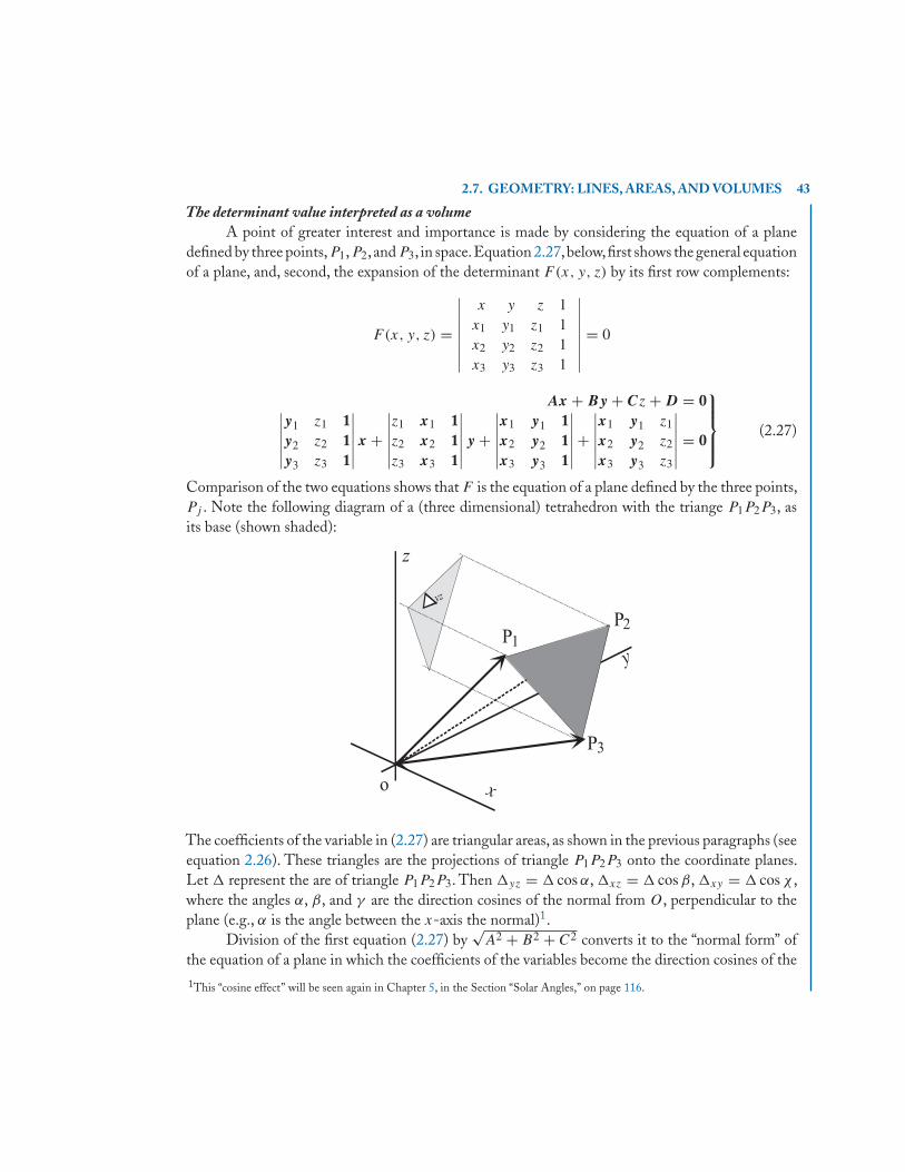
2.7. GEOMETRY: LINES, AREAS, AND VOLUMES 43
The determinant value interpreted as a volumeA point of greater interest and importance is made by considering the equation of a plane
defined by three points,P1,P2, andP3, in space.Equation 2.27,below,first shows the general equationof a plane, and, second, the expansion of the determinant F(x, y, z) by its first row complements:
F(x, y, z) =
∣∣∣∣∣∣∣∣x y z 1
x1 y1 z1 1x2 y2 z2 1x3 y3 z3 1
∣∣∣∣∣∣∣∣= 0
Ax + By + Cz + D = 0∣∣∣∣∣∣y1 z1 1y2 z2 1y3 z3 1
∣∣∣∣∣∣ x +∣∣∣∣∣∣z1 x1 1z2 x2 1z3 x3 1
∣∣∣∣∣∣ y +∣∣∣∣∣∣x1 y1 1x2 y2 1x3 y3 1
∣∣∣∣∣∣+∣∣∣∣∣∣x1 y1 z1
x2 y2 z2
x3 y3 z3
∣∣∣∣∣∣ = 0
⎫⎪⎪⎬⎪⎪⎭ (2.27)
Comparison of the two equations shows that F is the equation of a plane defined by the three points,Pj . Note the following diagram of a (three dimensional) tetrahedron with the triange P1P2P3, asits base (shown shaded):
The coefficients of the variable in (2.27) are triangular areas, as shown in the previous paragraphs (seeequation 2.26). These triangles are the projections of triangle P1P2P3 onto the coordinate planes.Let � represent the are of triangle P1P2P3. Then �yz = � cos α, �xz = � cos β, �xy = � cos χ ,where the angles α, β, and γ are the direction cosines of the normal from O, perpendicular to theplane (e.g., α is the angle between the x-axis the normal)1.
Division of the first equation (2.27) by√
A2 + B2 + C2 converts it to the “normal form” ofthe equation of a plane in which the coefficients of the variables become the direction cosines of the1This “cosine effect” will be seen again in Chapter 5, in the Section “Solar Angles,” on page 116.
44 2. DETERMINANTS
normal, and the constant term the distance from O to the plane—the length, p, of the normal. Thatis:
p = −D√A2 + B2 + C2
. (2.28)
The volume of this tetrahedron is given as 13×area of the base(triangle P1P2P3) × the length of the
normal to the plane.Noting that A, B, and C are related to the areas of the projected triangle (e.g., A = 2�yz), then
√A2 + B2 + C2 = 2
√�2
yz + �2zx + �2
xy = 2�
√cos2 α + cos2 β + cos2 γ = 2� .
The term√
cos2 α + cos2 β + cos2 γ = 1, the direction cosines are the coordinates of a “unit vector.”Therefore,
volume = 1
3p × � = 1
3
D√A2 + B2 + C2
×√
A2 + B2 + C2
2= 1
6
∣∣∣∣∣∣x1 y1 z1
x2 y2 z2
x3 y3 z3
∣∣∣∣∣∣D is the value of the determinant defined by the vectors OPi , the constant term in F(x, y, z).
This important result shows that the value of a determinant can be equated to a “volume.” Inmore than 3 dimensions, the volume cannot be visualized—but, just envision the 3 dimensional caseand let the mathematics take over for larger dimensionality.
A determinant (its expanded value) can become very small just because its vectors (rows orcolumns) are themselves small, or a subset of them is small. This will be easy to see, and can bechanged by re-scaling, making its rows balanced in size numerically.
After rescaling, the value of the determinant becomes a measure of its “skew”—the orientationof vectors within the set. For example, in the present case, if the point P1 were to move toward theline P2P3, the volume of the tetrahedron would decrease. At the limit, if P1 reaches this line thenOP1 falls into the plane defined by the other two vectors—the volume, and hence the determinantvalue, will be zero. At the other extreme, these vectors could be mutually orthogonal, minimum“skew.”
2.8 THE ADJOINT AND INVERSE MATRICESThe adjoint matrix—defined in Section 2.6, page 38 as the transpose of the matrix of cofactors—isdenoted as Aa or Aadj. Equation (2.18) leads directly to the statement of (2.29):
AAa = ∣∣A∣∣ I, for any square matrix. (2.29)
[A] Aa∣∣A∣∣ = I, when |A| �= 0 . (2.30)
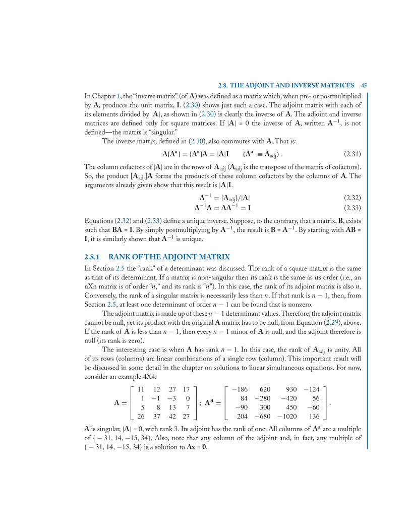
2.8. THE ADJOINT AND INVERSE MATRICES 45
In Chapter 1, the “inverse matrix” (of A) was defined as a matrix which, when pre- or postmultipliedby A, produces the unit matrix, I. (2.30) shows just such a case. The adjoint matrix with each ofits elements divided by |A|, as shown in (2.30) is clearly the inverse of A. The adjoint and inversematrices are defined only for square matrices. If |A| = 0 the inverse of A, written A−1, is notdefined—the matrix is “singular.”
The inverse matrix, defined in (2.30), also commutes with A. That is:
A[Aa] = [Aa]A = |A|I (Aa ≡ Aadj) . (2.31)
The column cofactors of |A| are in the rows of Aadj (Aadj is the transpose of the matrix of cofactors).So, the product [Aadj]A forms the products of these column cofactors by the columns of A. Thearguments already given show that this result is |A|I.
A−1 = [Aadj]/|A| (2.32)A−1A = AA−1 = I (2.33)
Equations (2.32) and (2.33) define a unique inverse. Suppose, to the contrary, that a matrix, B, existssuch that BA = I. By simply postmultiplying by A−1, the result is B = A−1. By starting with AB =I, it is similarly shown that A−1 is unique.
2.8.1 RANK OF THE ADJOINT MATRIXIn Section 2.5 the “rank” of a determinant was discussed. The rank of a square matrix is the sameas that of its determinant. If a matrix is non-singular then its rank is the same as its order (i.e., annXn matrix is of order “n,” and its rank is “n”). In this case, the rank of its adjoint matrix is also n.Conversely, the rank of a singular matrix is necessarily less than n. If that rank is n − 1, then, fromSection 2.5, at least one determinant of order n − 1 can be found that is nonzero.
The adjoint matrix is made up of these n − 1 determinant values.Therefore, the adjoint matrixcannot be null, yet its product with the original A matrix has to be null, from Equation (2.29), above.If the rank of A is less than n − 1, then every n − 1 minor of A is null, and the adjoint therefore isnull (its rank is zero).
The interesting case is when A has rank n − 1. In this case, the rank of Aadj is unity. Allof its rows (columns) are linear combinations of a single row (column). This important result willbe discussed in some detail in the chapter on solutions to linear simultaneous equations. For now,consider an example 4X4:
A =
⎡⎢⎢⎣
11 12 27 171 −1 −3 05 8 13 7
26 37 42 27
⎤⎥⎥⎦ ; Aa =
⎡⎢⎢⎣
−186 620 930 −12484 −280 −420 56
−90 300 450 −60204 −680 −1020 136
⎤⎥⎥⎦ .
A is singular, |A| = 0, with rank 3. Its adjoint has the rank of one. All columns of Aa are a multipleof { − 31, 14, −15, 34}. Also, note that any column of the adjoint and, in fact, any multiple of{ − 31, 14, −15, 34} is a solution to Ax = 0.
46 2. DETERMINANTS
2.9 DETERMINANT EVALUATION
The foregoing lays out the characteristics and properties of determinants, but implies very labori-ous work in actually calculating their values. Fortunately, this is not the case. Modern methods ofexpansion are straightforward, and easy to program. They do involve a lot of calculation but far lessthan the direct methods already discussed.
Practical evaluation of determinants involves some method of condensation (i.e., reductionto a lower order of determinant). Repeated applications of the method eventually lead to the scalarresult, |A|.These methods are equivalent to the “elimination of xj ,” as discussed in the very beginningof this chapter.The array concept of the determinant lends itself to the definition of arrays in popularprogramming languages, and the “repeated applications” mentioned above lead to program looping.
2.9.1 PIVOTAL CONDENSATION“Pivotal condensation” is a name more difficult than the method. The idea is easily described, easilyunderstood, easily done—and fun to program.The description here will be via example using a 4X4:
∣∣∣∣∣∣∣∣a11 a12 a13 a14
a21 a22 a23 a24
a31 a32 a33 a34
a41 a42 a43 a44
∣∣∣∣∣∣∣∣= ±d
∣∣∣∣∣∣∣∣b11 b12 b13 b14
0 0 1 0b31 b32 b33 b34
b41 b42 b43 b44
∣∣∣∣∣∣∣∣= −d
∣∣∣∣∣∣b11 b12 b14
b31 b32 b34
b41 b42 b44
∣∣∣∣∣∣ . (2.34)
The determinant |A| is manipulated to produce an equivalent d|B|. The determinant |B| in (2.34)can be expanded by the elements of its second row. The result will clearly be a determinant of3rd order as shown. A minus sign is chosen, in this case, because of the factor (−1)(2+3) resultingfrom having chosen the 2,3 element as the “pivot,” The resulting “condensed” determinant is thenoperated upon in the same manner to produce further condensations until the product string of d
factors multiply to the final result.In this example, the second row is arbitrarily chosen for the first “pivot row.” Rather than
make an arbitrary choice, the largest element (absolute value) is chosen as the pivotal element. Thepivot does not have to be the largest, but that’s a good choice—and avoids the possible choice of apivot equal to zero. If the matrix is complex, just choose the element, x + jy, with the largest sumof absolute values of real and imaginary parts (|x| + |y|).
At the beginning step in each cycle, let the pivot (largest) element be apq . If the pth row isdivided by this value, the new pqth element will have the value 1.0. In the equivalent d|B|, the factord is set equal to apq , (determinant property 4, in Section 2.4). Now, from each column the propermultiple of column q is subtracted such that all elements of row p become zero. These operationsdo not change the value of the determinant (by property 8). In the column subtractions it is notnecessary to actually calculate the values in row p, since it is already known that they will be zeros.Also, column q remains the same—is skipped from calculations. The new, condensed determinantdoes not take any of its elements from the pth row, or qth column of |B|
2.9. DETERMINANT EVALUATION 47
Condensing the determinant uses Equation (2.13), expansion by first minors.The minus signis taken if the cofactor has the opposite sign from the minor, as in (2.14), i.e., (−1)(p+q).
2.9.2 GAUSSIAN REDUCTIONThe foregoing paragraphs indicate that determinant evaluation amounts to the repeated applicationof a simple algorithm. Gaussian reduction is one of these simple algorithms, and it is not verydifferent than pivotal condensation. As it progresses, the determinant is condensed to a smaller andsmaller array until the determinant value becomes the product of n factors (and these factors are the“pivots,” just as before).
The objective of Gaussian Reduction is to reduce the given determinant to an equivalenttriangular one like the following: ∣∣∣∣∣∣∣∣
a11 a12 a13 a14
0 a22 a23 a24
0 0 a33 a34
0 0 0 a44
∣∣∣∣∣∣∣∣4x4 upper triangular determinant
Its value is easily seen to be equal to the product of its main diagonal elements. All other termscontain the zero as a factor. The pivots, then, are these aii elements.
As before, at each stage, the pivots chosen are the largest elements in the condensed deter-minant. In general, of course, these are not found on the main diagonal. They must be moved thereby row and column exchanges. If both a row and a column exchange occur, the determinant value isnot changed. As an example: at the first stage the largest element is found to be a34. To bring thiselement to the a11 position, row three is exchanged with row one and column four is exchangedwith column one. Since two sign changes are made, they cancel. If only one (either column or row)exchange occurs, the value of the determinant changes sign. Thus, it is necessary to keep track ofthese exchanges.
After the exchange(s) occur the method is very like pivotal condensation, except it is notdesired to divide the pivotal row by the pivot (to reduce the pivot position to unity). But, the rest ofthe pivotal column is reduced to zero, just as the pivotal rows were reduced in the previous method.
∣∣A∣∣ =
∣∣∣∣∣∣∣∣a11 a12 · · · a1n
0 c22 · · · · · ·0 ck2 ckk
0 . . . cnn
∣∣∣∣∣∣∣∣ cij = aij − a1jai1a11
ij = 2, 3 · · · nThe above display shows the first stage, after the largest element has been moved to the a11 position.If we make the calculations indicated, the elements in the first column become zero:
At j = 1; cij = aij − ai1
a11a1j = ai1 − ai1
a11a11 = 0
48 2. DETERMINANTS
and the condensed determinant is |cij |. In (row) vector terms, the elements cij are formed bysubtracting from each ith row the proper multiple of the pivot row (row 1, in stage 1):
[ci] = [ai] − ai1
a11[a1] . (2.35)
In (2.35) the boldface type identifies vectors and the square brackets indicate [row] vectors, not{column} vectors.The method is:
(1) Set p = 1; p is defined as the pivot row index. As such, it will take values 1..n (n is the orderof the determinant). The pivots, then will have the subscripts pp.
(2) Find the element with the largest absolute value (if the determinant is complex, the absolutevalue could be used, or just the largest sum of abs values of real and imaginary parts).
Exchange rows and columns to move the largest element to the a′pp position. The “prime” is
used here to indicate that the values of these elements change as the procedure continues.
(3) Now, for all i rows below the pth, subtracta′ip
a′pp
times the pth row, as in (2.35). Note that it is
unnecessary to operate on elements in, or to the left of, the pth column. They will all be zero.
(4) Now, increment p. If this new value is less than n, then repeat steps 2 and 3. If p = n, theprocedure is complete. The determinant can now be evaluated as the product of the diagonalelements.
The method can become confusing with the exchange of rows and columns. Otherwise, it is quitestraightforward. The labor is alleviated by the use of a computer; and the programming is enjoyable,tricky only in keeping track of row/column exchanges.
In this regard, it is unnecessary to actually exchange data rows/columns. Lists can be kept,indicating where they are. For example, evaluating a 4X4, the row list:
row list = rlist(i) = 1,2,3,4. If rows 2 and 4 are exchanged, rlist(i) = 1,4,3,2 .
The same thing can be said for the column list.Of course, this leads to the complication that the elements must be accessed through these
lists. That is, an element a(i, j), in |A|, now must be referred to as a(rlist(i), clist(j)).The Gaussian Reduction method can be done using “partial pivoting,” in which the pivot
elements are always chosen from the pivot column. This reduces the exchanges down to just rowinterchanges. Within the subject at hand, full pivoting is just as easy. The advantage (reduced com-plexity) of partial pivoting is noticeable in solving simultaneous equations, and/or calculating theinverse of a matrix. There will be more about this in the following chapter.
The reduction of a 5X5 will provide an example. At each stage, the new pivot is shown withina box. In each case the pivot is the largest element within the condensed matrix. At stage 1, the
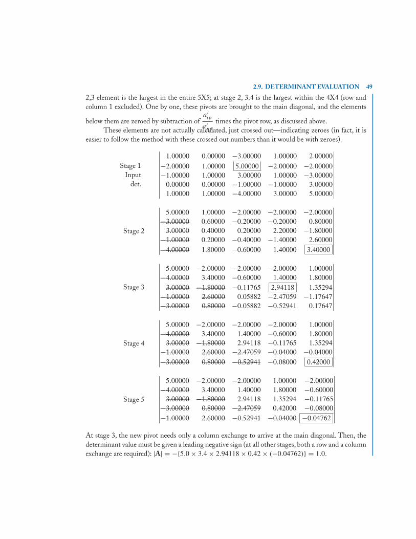
2.9. DETERMINANT EVALUATION 49
2,3 element is the largest in the entire 5X5; at stage 2, 3.4 is the largest within the 4X4 (row andcolumn 1 excluded). One by one, these pivots are brought to the main diagonal, and the elements
below them are zeroed by subtraction ofa′ip
a′pp
times the pivot row, as discussed above.These elements are not actually calculated, just crossed out—indicating zeroes (in fact, it is
easier to follow the method with these crossed out numbers than it would be with zeroes).
Stage 1Input
det.
∣∣∣∣∣∣∣∣∣∣∣
1.00000 0.00000 −3.00000 1.00000 2.00000
−2.00000 1.00000 5.00000 −2.00000 −2.00000−1.00000 1.00000 3.00000 1.00000 −3.00000
0.00000 0.00000 −1.00000 −1.00000 3.000001.00000 1.00000 −4.00000 3.00000 5.00000
∣∣∣∣∣∣∣∣∣∣∣
Stage 2
∣∣∣∣∣∣∣∣∣∣∣
5.00000 1.00000 −2.00000 −2.00000 −2.00000−3.00000 0.60000 −0.20000 −0.20000 0.80000
3.00000 0.40000 0.20000 2.20000 −1.80000−1.00000 0.20000 −0.40000 −1.40000 2.60000−4.00000 1.80000 −0.60000 1.40000 3.40000
∣∣∣∣∣∣∣∣∣∣∣
Stage 3
∣∣∣∣∣∣∣∣∣∣∣
5.00000 −2.00000 −2.00000 −2.00000 1.00000−4.00000 3.40000 −0.60000 1.40000 1.80000
3.00000 −1.80000 −0.11765 2.94118 1.35294−1.00000 2.60000 0.05882 −2.47059 −1.17647−3.00000 0.80000 −0.05882 −0.52941 0.17647
∣∣∣∣∣∣∣∣∣∣∣
Stage 4
∣∣∣∣∣∣∣∣∣∣∣
5.00000 −2.00000 −2.00000 −2.00000 1.00000−4.00000 3.40000 1.40000 −0.60000 1.80000
3.00000 −1.80000 2.94118 −0.11765 1.35294−1.00000 2.60000 −2.47059 −0.04000 −0.04000−3.00000 0.80000 −0.52941 −0.08000 0.42000
∣∣∣∣∣∣∣∣∣∣∣
Stage 5
∣∣∣∣∣∣∣∣∣∣∣
5.00000 −2.00000 −2.00000 1.00000 −2.00000−4.00000 3.40000 1.40000 1.80000 −0.60000
3.00000 −1.80000 2.94118 1.35294 −0.11765−3.00000 0.80000 −2.47059 0.42000 −0.08000
−1.00000 2.60000 −0.52941 −0.04000 −0.04762
∣∣∣∣∣∣∣∣∣∣∣At stage 3, the new pivot needs only a column exchange to arrive at the main diagonal. Then, thedeterminant value must be given a leading negative sign (at all other stages, both a row and a columnexchange are required): |A| = −{5.0 × 3.4 × 2.94118 × 0.42 × (−0.04762)} = 1.0.
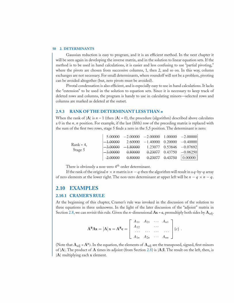
50 2. DETERMINANTS
Gaussian reduction is easy to program, and it is an efficient method. In the next chapter itwill be seen again in developing the inverse matrix, and in the solution to linear equation sets. If themethod is to be used in hand calculations, it is easier and less confusing to use “partial pivoting,”where the pivots are chosen from successive columns, 1, then 2, and so on. In this way, columnexchanges are not necessary. For small determinants, where roundoff will not be a problem, pivotingcan be avoided altogether (but, zero pivots must be avoided).
Pivotal condensation is also efficient, and is especially easy to use in hand calculations. It lacksthe “extension” to be used in the solution to equation sets. Since it is necessary to keep track ofdeleted rows and columns, the program is handy to use in calculating minors—selected rows andcolumns are marked as deleted at the outset.
2.9.3 RANK OF THE DETERMINANT LESS THAN n
When the rank of |A| is n – 1 (then |A| = 0), the procedure (algorithm) described above calculatesa 0 in the n, n position. For example, if the last (fifth) row of the preceding matrix is replaced withthe sum of the first two rows, stage 5 finds a zero in the 5,5 position. The determinant is zero:
Rank = 4,Stage 5
∣∣∣∣∣∣∣∣∣∣∣
5.00000 −2.00000 −2.00000 1.00000 −2.00000−1.00000 2.60000 −1.40000 0.20000 −0.40000−3.00000 −1.80000 1.23077 0.53846 −0.07692−3.00000 0.80000 0.23077 0.43750 −0.06250
2.00000 0.80000 0.23077 0.43750 0.00000
∣∣∣∣∣∣∣∣∣∣∣There is obviously a non-zero 4th order determinant.If the rank of the original n × n matrix is n − q then the algorithm will result in a q-by-q array
of zero elements at the lower right. The non-zero determinant at upper left will be n − q × n − q.
2.10 EXAMPLES2.10.1 CRAMER’S RULEAt the beginning of this chapter, Cramer’s rule was invoked in the discussion of the solution tothree equations in three unknowns. In the light of the later discussion of the “adjoint” matrix inSection 2.8, we can revisit this rule. Given the n-dimensional Ax = c, premultiply both sides by Aadj.
AaAx = ∣∣A∣∣ x = Aac =
⎡⎢⎢⎣
A11 A21 · · · An1
A12 · · ·· · · · · · · · · · · ·
A1n A2n · · · Ann
⎤⎥⎥⎦ {c} .
(Note that Aadj = Aa). In the equation, the elements of Aadj are the transposed, signed, first minorsof |A|. The product of A times its adjoint (from Section 2.8) is |A|I. The result on the left, then, is|A| multiplying each x element.
2.10. EXAMPLES 51
Looking at x1 for example, |A|x1 = A11c1 + A21c2 + · · · + An1cn. But, the expression onthe right is just the LaPlace expansion of |A| with its first column replaced by the {c} vector.
Then, each xi is obtained as the ratio of two determinants.The determinant in the numeratoris |A| with its ith column replaced by the {c} vector, and the denominator is |A| itself. This isCramer’s rule.
2.10.2 AN EXAMPLE COMPLEX DETERMINANTIn Chapter 1 the sum of two matrices is given as the sum of the individual elements. Then
C = [aik + jbik] = A + jB
and we can think of the matrix as a single one with complex elements or as two separate matrices.(Note that the notation j = √−1 “interferes with” the notation of referring to columns with thesubscript “j ”).
The objective in this example is to determine |C| = | aik + jbik |. If the routine availablehandles complex numbers, then |C| is evaluated without further complication. But, it is possible toevaluate |C| using only real arithmetic. This will be illustrated in the simplest case—a 2X2.
We will use “vector notation” |C| = |c1c2|.
ck ={
a1k + jb1k
a2k + jb2k
}={
a1k
a2k
}+ j
{b1k
b2k
}= ak + jbk .
Now, using determinant property 7:
| c1c2 | = | a1c2 | + j∣∣ b1c2
∣∣| a1c2 | = | a1a2 | + j
∣∣ a1b2∣∣
j∣∣ b1c2
∣∣ = j∣∣ b1a2
∣∣− ∣∣ b1b2∣∣
and therefore | C | = | a1a2 | − ∣∣ b1b2∣∣+ j
{∣∣ a1b2∣∣+ ∣∣ b1a2
∣∣}.The same method can be used in expanding any complex nXn determinant. The result will
be 2n determinants to expand, but, at least they will be real.
2.10.3 THE “CHARACTERISTIC DETERMINANT”Associated with a matrix A(nXn) is a special determinant with a single variable, usually denoted λ.The matrix A(λ) = A − λI is simply formed by subtracting λ from its main diagonal elements. Thedeterminant of A(λ) is an nth order polynomial in the parameter. Again using a 2X2:
∣∣A(λ)∣∣ =
∣∣∣∣ a11 − λ a12
a21 a22 − λ
∣∣∣∣ .
52 2. DETERMINANTS
In this particular case, the use of property 7 is “the hard way,” but for higher order determinants itis easier, and can be programmed.∣∣∣∣ a11 − λ a12
a21 a22 − λ
∣∣∣∣ =∣∣∣∣ a11 a12
a21 a22
∣∣∣∣−∣∣∣∣ a11 0
a21 λ
∣∣∣∣−∣∣∣∣ λ a12
0 a22
∣∣∣∣+∣∣∣∣ λ 0
0 λ
∣∣∣∣ .
The “characteristic polynomial” is, then: p(λ) = λ2 − (a11 + a22)λ + ∣∣A∣∣.2.11 EXERCISES
2.1. Find the inversions in the digit sequences below:
5741326 35421 123465 654321.
2.2. Determine which of the terms, below, are terms in the expansion of a determinant. Forthose that are legal, determine the leading sign.
a34a33a14a21 a41a32a21a14a55 b13b24b33b42 b44b12b31b23 c43c22c14c51c35 .
2.3. Expand the following determinants
A =∣∣∣∣∣∣
3 1 20 −4 1
−1 2 −2
∣∣∣∣∣∣ B =
∣∣∣∣∣∣∣∣1 2 3 40 1 2 30 2 0 10 3 0 5
∣∣∣∣∣∣∣∣2.4. Expand |B|, above, using 2X2 complements from rows 3 and 4.
2.5. Expand |B| above by completing its transformation to triangular form.
2.6. Expand |A| above using pivotal condensation.
2.7. Given A and B: A =
⎡⎢⎢⎣
1 30 −12 21 4
⎤⎥⎥⎦ and B =
[2 −3 0 1
−1 1 2 −2
].
Find |A B| and |B A|.
2.8. Expand the determinant C =∣∣∣∣∣∣a11 + jb11 a12 + jb12 a13 + jb13
a21 + jb21 a22 + jb22 a23 + jb23
a31 + jb31 a32 + jb32 a33 + jb33
∣∣∣∣∣∣Use the method given in Section 2.10.2.
2.11. EXERCISES 53
2.9. Given A(12X12). How many terms are in the term-by term expansion of |A|? How manyfactors are in each term? How long would it take your PC to calculate |A|, term-by-term?
2.10. A (5X5) determinant is to be expanded by complements from its first 3 rows. One suchcomplement is∣∣∣∣∣∣
a11 a13 a14
a21 a23 a24
a31 a33 a34
∣∣∣∣∣∣ . What leading sign should be placed on this term?
2.11. Determine the rank of the matrix A1
A1 =
⎡⎢⎢⎣
1 2 3 42 4 6 83 6 9 124 8 12 16
⎤⎥⎥⎦ A2 =
⎡⎢⎢⎣
5 −3 11 −5−2 0 −4 1−1 −3 −1 −2
3 3 5 1
⎤⎥⎥⎦ .
2.12. Using Gaussian Reduction methods, reduce A2 to triangle form, and determine its rank.Use “partial pivoting” (i.e., select pivots such that column interchanges are not required).
2.13. Given a 3X3 determinant made up of differentiable functions yij (x), show that the derivativeof the determinant is given by:
d
dx
∣∣ y1y2y3∣∣ = ∣∣y′
1y2y3∣∣+ ∣∣ y1y′
2y3∣∣+ ∣∣ y1y2y′
3
∣∣ ;yj =
⎧⎨⎩
y1j
y2j
y3j
⎫⎬⎭ ; and
dyj
dx= y′
j =
⎧⎪⎨⎪⎩
y′1j
y′2j
y′3j
⎫⎪⎬⎪⎭ .

55
C H A P T E R 3
Matrix Inversion
3.1 INTRODUCTIONThis chapter will discuss matrix inversion, and the very closely related subject of the solution ofsimultaneous equation sets. The inversion matrix arrays will necessarily be square, (nXn), for whichthe inversion process is defined — and for which the determinant is defined.
Emphasis is placed on the mechanical methods used in the inversion process. The next chap-ter will consider simultaneous equation sets as “vector transformations,” and is oriented toward ageometric interpretation, and considerations of compatibility.
In Chapter 2, Section 2.8, it was shown that a square matrix, whose determinant, |A|, is otherthan zero, possesses an “inverse matrix,” A−1, such that:
A−1A = AA−1 = I (3.1)
where I is defined as the (nXn) unit matrix. The elements of the inverse matrix are the “cofactors”of A divided by |A|; the cofactors being arranged into the “adjoint matrix.”
A−1 = [Aadj]/|A| (|A| �= 0) . (3.2)
The adjoint matrix is the transpose of the matrix of cofactors; its columns contain the row cofactorsof A. The cofactor of aij is the signed first minor of aij , the leading sign being determined negativeif i + j is odd, positive if it is even. Then, the inverse matrix is composed entirely of determinants;the minor is the (n-1Xn-1) determinant formed by deleting the row and column of the aij term.Therefore, the inverse could be determined by this definition.But, these calculations are quite lengthy.Instead, pivotal reduction methods will be discussed — including the Gauss Reduction which wasdiscussed in the previous chapter. This simple method will be shown to be an amazingly effectivetool for inverting matrices and solving simultaneous linear equations.
As a preliminary step, the “elementary transformation matrices” (Chapter 1, Section 1.4) willbe revisited, to provide further insight, and some justification for later methods.
3.2 ELEMENTARY OPERATIONS IN MATRIX FORMThree elementary operations were used in the previous chapter, in diagonalizing a determinant.Theyare: (1) To any row (column) is added a multiple of another row (column). (2) A row (column) isdivided by some factor. (3) Two rows (columns) are interchanged (this occurs when a pivot elementis brought to the main diagonal). These operations can be put into matrix form.
56 3. MATRIX INVERSION
Operation 1. Q ij (k). Starting with the (nXn) unit matrix, replace the ijth element (i �= j) with afactor kij . Now if a matrix, A, is premultiplied by this “transform” matrix:
Qij (k)A = B; i �= j . (3.3)
The matrix B is the same as A, except that to its ith row is added k times its j th row. Note the 3X3example Q 23(k):⎡
⎣ 1 0 00 1 k
0 0 1
⎤⎦⎡⎣ 3 1 2
0 2 -11 -1 2
⎤⎦ =
⎡⎣ 3 1 2
0 + k 2 − k −1 + 2k
1 −1 2
⎤⎦ . (3.4)
The reader should try other examples – with the factor k in all the nondiagonal locations of Q ij .Note that in every case (wherever the k factor is — as long as it is not on the main diagonal),
the determinant, |Q ij |, is 1. Furthermore, from the previous chapter on determinants, the value of|A| is unchanged by this fundamental operation, i.e., |B| = |Q ij ||A| = |A|.
Now, in the case B = AQ ij (k), (postmultiplication of A by the same type of transformation):⎡⎣ 3 1 2
0 2 -11 -1 2
⎤⎦⎡⎣ 1 0 0
0 1 k
0 0 1
⎤⎦ =
⎡⎣ 3 1 2 + k
0 2 −1 + 2k
1 −1 2 − k
⎤⎦ . (3.5)
In this case, to the j th column is added k times the ith column – where i and j are the row, columnpositions of k. Note the difference, compared to premultiplication.
Again note that |Q ij | = 1, and that |A| = |B|.Operation 2. Q j (k): Beginning with the unit matrix, replace the j th main diagonal element with afactor, k. It should be obvious that premultiplying A with this Q j (k) will multiply elements of thej th row of A by k:
Q2(k)
⎡⎣ 1 0 0
0 k 00 0 1
⎤⎦⎡⎣ 3 1 2
0 2 -11 -1 2
⎤⎦ =
⎡⎣ 3 1 2
0 × k 2 × k −1 × k
1 −1 2
⎤⎦ (3.6)
and, in postmultiplication the j th column is multiplied:⎡⎣ 3 1 2
0 2 −11 −1 2
⎤⎦⎡⎣ 1 0 0
0 1 00 0 k
⎤⎦ =
⎡⎣ 3 1 2 × k
0 2 −1 × k
1 −1 2 × k
⎤⎦ . (3.7)
In this case, |Q j (k)| = k, and |B| = |Q j (k)||A| = k|A|.Operation 3. Q i∼j . Interchange row (or column) i with row (or column) j of the unit matrix. Now,premultiply A by this Q matrix:⎡
⎣ 0 0 10 1 01 0 0
⎤⎦⎡⎣ 3 1 2
0 2 -11 -1 2
⎤⎦ =
⎡⎣ 1 −1 2
0 2 −13 1 2
⎤⎦ . (3.8)
3.2. ELEMENTARY OPERATIONS IN MATRIX FORM 57
In this case, with Q i∼j formed by interchanging rows one and three of the unit matrix, the resultof B = Q i∼j A is that the same rows of A are interchanged. In postmultiplication:⎡
⎣ 3 1 20 2 −11 −1 2
⎤⎦⎡⎣ 1 0 0
0 0 10 1 0
⎤⎦ =
⎡⎣ 3 2 1
0 −1 21 2 −1
⎤⎦ . (3.9)
Not surprisingly, in this case, with rows (columns) 2 and 3 of I interchanged, these same columnsof A are interchanged.
The determinant |Q i∼j | = –1, and |B| = –|A|. This is analogous to the property that inter-changing two rows (columns) of a matrix changes the sign of the determinant.
3.2.1 DIAGONALIZATION USING ELEMENTARY MATRICESThe diagonalization or triangularization of a matrix, A, can be accomplished by a series of theseelementary operations. These, in turn, can be visualized as pre-, and/or postmultiplication of A bythe elementary transform matrices. Note: In the equations below, the symbol Q is used withoutindication of its type. This is done so that the final transformation is more clearly shown as theproduct of the individual operations.
B = QA (3.10)
where Q = Q mQ m−1 .. Q 2Q 1 (a series of m elementary operations, each of which is of a typediscussed above) and B is, optionally, diagonal, or triangular. Then
A−1Q−1 = B−1, and therefore (3.11)A−1 = B−1Q . (3.12)
The B matrix, whether diagonal or triangular, is easy to invert. The Q matrix is developed duringthe procedure — and note that its inverse is not required . Then, the method is a good learning tool,it provides the basis for the very practical inversion tools, and is not an unreasonable one to use forsmall matrices, by hand.
As an example of the method, the (3X3) used above, as the A matrix, will be transformed, bymeans of a premultiplier Q matrix, to diagonal form. The Q matrices are:
Q 31(–1/3); Unit matrix with element (3,1) replaced with –1/3; changes the 3rd row of A to[0 4/3 −4/3
]Q 32(2/3); Unit matrix with element (3,2) replaced with 2/3; changes the 3rd row of A to[
0 0 2/3]
Q 12(–1/2); Unit matrix with element (1,2) replaced with –1/2; changes the 1st row of A to[3 0 5/2
]
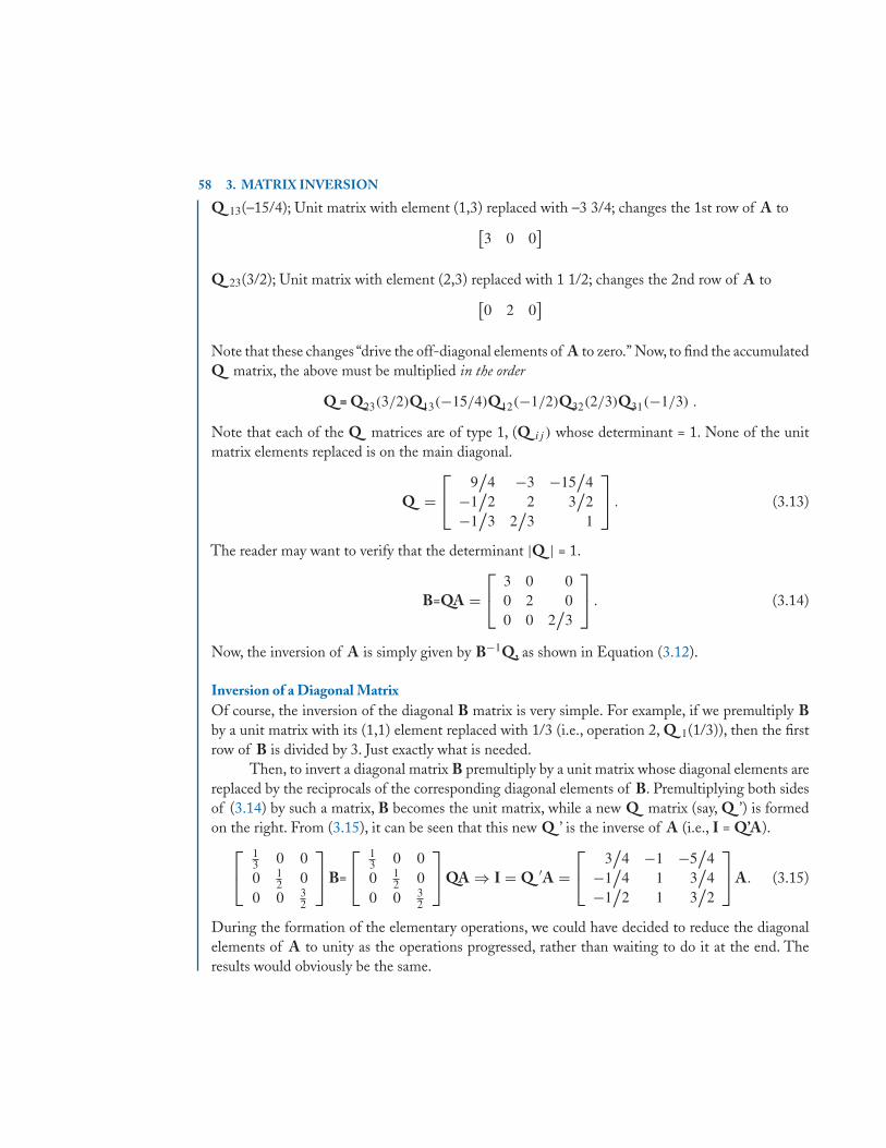
58 3. MATRIX INVERSION
Q 13(–15/4); Unit matrix with element (1,3) replaced with –3 3/4; changes the 1st row of A to[3 0 0
]Q 23(3/2); Unit matrix with element (2,3) replaced with 1 1/2; changes the 2nd row of A to[
0 2 0]
Note that these changes “drive the off-diagonal elements of A to zero.” Now, to find the accumulatedQ matrix, the above must be multiplied in the order
Q = Q23(3/2)Q13(−15/4)Q12(−1/2)Q32(2/3)Q31(−1/3) .
Note that each of the Q matrices are of type 1, (Q ij ) whose determinant = 1. None of the unitmatrix elements replaced is on the main diagonal.
Q =⎡⎣ 9
/4 −3 −15
/4
−1/
2 2 3/
2−1
/3 2
/3 1
⎤⎦ . (3.13)
The reader may want to verify that the determinant |Q | = 1.
B=QA =⎡⎣ 3 0 0
0 2 00 0 2
/3
⎤⎦ . (3.14)
Now, the inversion of A is simply given by B−1Q, as shown in Equation (3.12).
Inversion of a Diagonal MatrixOf course, the inversion of the diagonal B matrix is very simple. For example, if we premultiply Bby a unit matrix with its (1,1) element replaced with 1/3 (i.e., operation 2, Q 1(1/3)), then the firstrow of B is divided by 3. Just exactly what is needed.
Then, to invert a diagonal matrix B premultiply by a unit matrix whose diagonal elements arereplaced by the reciprocals of the corresponding diagonal elements of B. Premultiplying both sidesof (3.14) by such a matrix, B becomes the unit matrix, while a new Q matrix (say, Q ’) is formedon the right. From (3.15), it can be seen that this new Q ’ is the inverse of A (i.e., I = Q’A).⎡
⎣ 13 0 00 1
2 00 0 3
2
⎤⎦B=
⎡⎣ 1
3 0 00 1
2 00 0 3
2
⎤⎦QA ⇒ I = Q ′A =
⎡⎣ 3
/4 −1 −5
/4
−1/
4 1 3/
4−1
/2 1 3
/2
⎤⎦A. (3.15)
During the formation of the elementary operations, we could have decided to reduce the diagonalelements of A to unity as the operations progressed, rather than waiting to do it at the end. Theresults would obviously be the same.
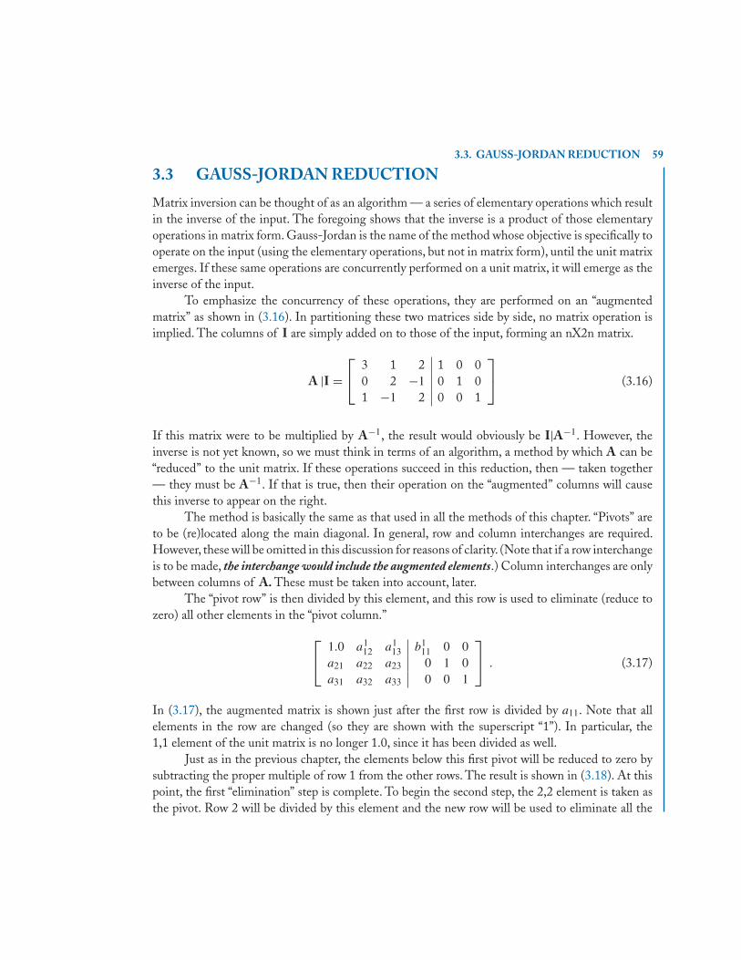
3.3. GAUSS-JORDAN REDUCTION 59
3.3 GAUSS-JORDAN REDUCTION
Matrix inversion can be thought of as an algorithm — a series of elementary operations which resultin the inverse of the input. The foregoing shows that the inverse is a product of those elementaryoperations in matrix form. Gauss-Jordan is the name of the method whose objective is specifically tooperate on the input (using the elementary operations, but not in matrix form), until the unit matrixemerges. If these same operations are concurrently performed on a unit matrix, it will emerge as theinverse of the input.
To emphasize the concurrency of these operations, they are performed on an “augmentedmatrix” as shown in (3.16). In partitioning these two matrices side by side, no matrix operation isimplied. The columns of I are simply added on to those of the input, forming an nX2n matrix.
A |I =⎡⎣ 3 1 2 1 0 0
0 2 −1 0 1 01 −1 2 0 0 1
⎤⎦ (3.16)
If this matrix were to be multiplied by A−1, the result would obviously be I|A−1. However, theinverse is not yet known, so we must think in terms of an algorithm, a method by which A can be“reduced” to the unit matrix. If these operations succeed in this reduction, then — taken together— they must be A−1. If that is true, then their operation on the “augmented” columns will causethis inverse to appear on the right.
The method is basically the same as that used in all the methods of this chapter. “Pivots” areto be (re)located along the main diagonal. In general, row and column interchanges are required.However, these will be omitted in this discussion for reasons of clarity. (Note that if a row interchangeis to be made, the interchange would include the augmented elements.) Column interchanges are onlybetween columns of A. These must be taken into account, later.
The “pivot row” is then divided by this element, and this row is used to eliminate (reduce tozero) all other elements in the “pivot column.”
⎡⎣ 1.0 a1
12 a113 b1
11 0 0a21 a22 a23 0 1 0a31 a32 a33 0 0 1
⎤⎦ . (3.17)
In (3.17), the augmented matrix is shown just after the first row is divided by a11. Note that allelements in the row are changed (so they are shown with the superscript “1”). In particular, the1,1 element of the unit matrix is no longer 1.0, since it has been divided as well.
Just as in the previous chapter, the elements below this first pivot will be reduced to zero bysubtracting the proper multiple of row 1 from the other rows. The result is shown in (3.18). At thispoint, the first “elimination” step is complete. To begin the second step, the 2,2 element is taken asthe pivot. Row 2 will be divided by this element and the new row will be used to eliminate all the
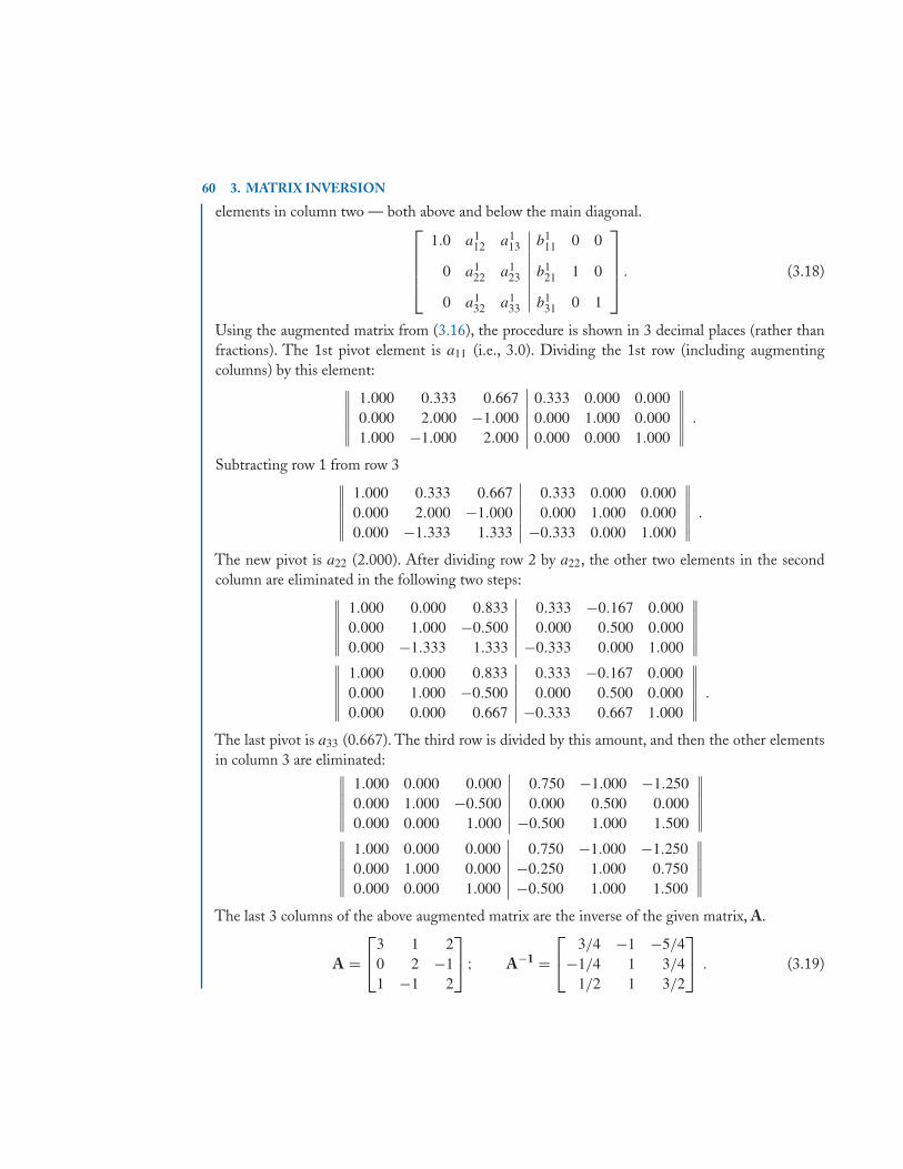
60 3. MATRIX INVERSION
elements in column two — both above and below the main diagonal.⎡⎢⎢⎢⎣
1.0 a112 a1
13 b111 0 0
0 a122 a1
23 b121 1 0
0 a132 a1
33 b131 0 1
⎤⎥⎥⎥⎦ . (3.18)
Using the augmented matrix from (3.16), the procedure is shown in 3 decimal places (rather thanfractions). The 1st pivot element is a11 (i.e., 3.0). Dividing the 1st row (including augmentingcolumns) by this element:∥∥∥∥∥∥
1.000 0.333 0.667 0.333 0.000 0.0000.000 2.000 −1.000 0.000 1.000 0.0001.000 −1.000 2.000 0.000 0.000 1.000
∥∥∥∥∥∥ .
Subtracting row 1 from row 3∥∥∥∥∥∥1.000 0.333 0.667 0.333 0.000 0.0000.000 2.000 −1.000 0.000 1.000 0.0000.000 −1.333 1.333 −0.333 0.000 1.000
∥∥∥∥∥∥ .
The new pivot is a22 (2.000). After dividing row 2 by a22, the other two elements in the secondcolumn are eliminated in the following two steps:∥∥∥∥∥∥
1.000 0.000 0.833 0.333 −0.167 0.0000.000 1.000 −0.500 0.000 0.500 0.0000.000 −1.333 1.333 −0.333 0.000 1.000
∥∥∥∥∥∥∥∥∥∥∥∥1.000 0.000 0.833 0.333 −0.167 0.0000.000 1.000 −0.500 0.000 0.500 0.0000.000 0.000 0.667 −0.333 0.667 1.000
∥∥∥∥∥∥ .
The last pivot is a33 (0.667). The third row is divided by this amount, and then the other elementsin column 3 are eliminated:∥∥∥∥∥∥
1.000 0.000 0.000 0.750 −1.000 −1.2500.000 1.000 −0.500 0.000 0.500 0.0000.000 0.000 1.000 −0.500 1.000 1.500
∥∥∥∥∥∥∥∥∥∥∥∥1.000 0.000 0.000 0.750 −1.000 −1.2500.000 1.000 0.000 −0.250 1.000 0.7500.000 0.000 1.000 −0.500 1.000 1.500
∥∥∥∥∥∥The last 3 columns of the above augmented matrix are the inverse of the given matrix, A.
A =⎡⎣3 1 2
0 2 −11 −1 2
⎤⎦ ; A−1 =
⎡⎣ 3/4 −1 −5/4
−1/4 1 3/41/2 1 3/2
⎤⎦ . (3.19)
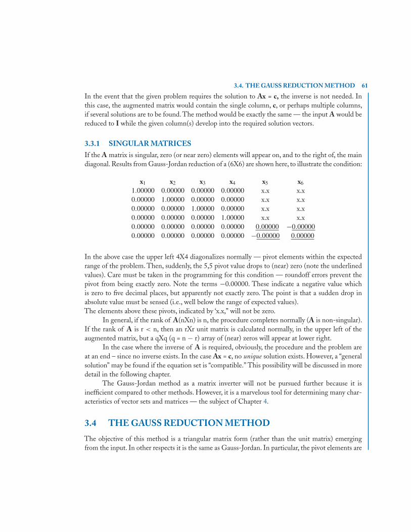
3.4. THE GAUSS REDUCTION METHOD 61
In the event that the given problem requires the solution to Ax = c, the inverse is not needed. Inthis case, the augmented matrix would contain the single column, c, or perhaps multiple columns,if several solutions are to be found. The method would be exactly the same — the input A would bereduced to I while the given column(s) develop into the required solution vectors.
3.3.1 SINGULAR MATRICESIf the A matrix is singular, zero (or near zero) elements will appear on, and to the right of, the maindiagonal. Results from Gauss-Jordan reduction of a (6X6) are shown here, to illustrate the condition:
x1 x2 x3 x4 x5 x6
1.00000 0.00000 0.00000 0.00000 x.x x.x0.00000 1.00000 0.00000 0.00000 x.x x.x0.00000 0.00000 1.00000 0.00000 x.x x.x0.00000 0.00000 0.00000 1.00000 x.x x.x0.00000 0.00000 0.00000 0.00000 0.00000 −0.000000.00000 0.00000 0.00000 0.00000 −0.00000 0.00000
In the above case the upper left 4X4 diagonalizes normally — pivot elements within the expectedrange of the problem. Then, suddenly, the 5,5 pivot value drops to (near) zero (note the underlinedvalues). Care must be taken in the programming for this condition — roundoff errors prevent thepivot from being exactly zero. Note the terms −0.00000. These indicate a negative value whichis zero to five decimal places, but apparently not exactly zero. The point is that a sudden drop inabsolute value must be sensed (i.e., well below the range of expected values).The elements above these pivots, indicated by ‘x.x,” will not be zero.
In general, if the rank of A(nXn) is n, the procedure completes normally (A is non-singular).If the rank of A is r < n, then an rXr unit matrix is calculated normally, in the upper left of theaugmented matrix, but a qXq (q = n − r) array of (near) zeros will appear at lower right.
In the case where the inverse of A is required, obviously, the procedure and the problem areat an end – since no inverse exists. In the case Ax = c, no unique solution exists. However, a “generalsolution” may be found if the equation set is “compatible.” This possibility will be discussed in moredetail in the following chapter.
The Gauss-Jordan method as a matrix inverter will not be pursued further because it isinefficient compared to other methods. However, it is a marvelous tool for determining many char-acteristics of vector sets and matrices — the subject of Chapter 4.
3.4 THE GAUSS REDUCTION METHOD
The objective of this method is a triangular matrix form (rather than the unit matrix) emergingfrom the input. In other respects it is the same as Gauss-Jordan. In particular, the pivot elements are
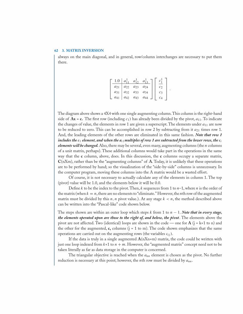
62 3. MATRIX INVERSION
always on the main diagonal, and in general, row/column interchanges are necessary to put themthere.
⎡⎢⎢⎣
1.0 a111 a1
12 a113
a21 a22 a23 a24
a31 a32 a33 a34
a41 a42 a43 a44
⎤⎥⎥⎦⎡⎢⎢⎢⎣
c11
c2
c3
c4
⎤⎥⎥⎥⎦ .
The diagram above shows a 4X4 with one single augmenting column.This column is the right-handside of Ax = c. The first row (including c1) has already been divided by the pivot, a11. To indicatethe changes of value, the elements in row 1 are given a superscript. The elements under a11 are nowto be reduced to zero. This can be accomplished in row 2 by subtracting from it a21 times row 1.And, the leading elements of the other rows are eliminated in this same fashion. Note that row 1includes the c1 element, and when the ai1multiples of row 1 are subtracted from the lower rows, the ci
elements will be changed. Also, there may be several, even many, augmenting columns (the n columnsof a unit matrix, perhaps). These additional columns would take part in the operations in the sameway that the c column, above, does. In this discussion, the c columns occupy a separate matrix,C(nXm), rather than be the “augmenting columns” of A. Today, it is unlikely that these operationsare to be performed by hand; so the visualization of the “side-by-side” columns is unnecessary. Inthe computer program, moving these columns into the A matrix would be a wasted effort.
Of course, it is not necessary to actually calculate any of the elements in column 1. The top(pivot) value will be 1.0, and the elements below it will be 0.0.
Define k to be the index to the pivot.Then, k sequences from 1 to n–1, where n is the order ofthe matrix (when k = n, there are no elements to “eliminate.” However, the nth row of the augmentedmatrix must be divided by this n, n pivot value.). At any stage k < n, the method described abovecan be written into the “Pascal-like” code shown below.
The steps shown are within an outer loop which steps k from 1 to n − 1. Note that in every stage,the elements operated upon are those to the right of, and below, the pivot . The elements above thepivot are not affected. Two (identical) loops are shown in the code — one for A (j = k+1 to n) andthe other for the augmented, c, columns (j = 1 to m). The code shown emphasizes that the sameoperations are carried out on the augmenting rows (the variables cij ).
If the data is truly in a single augmented A(nXn+m) matrix, the code could be written withjust one loop indexed from k+1 to n + m. However, the “augmented matrix” concept need not to betaken literally as far as data storage in the computer is concerned.
The triangular objective is reached when the ann element is chosen as the pivot. No furtherreduction is necessary at this point; however, the nth row must be divided by ann.
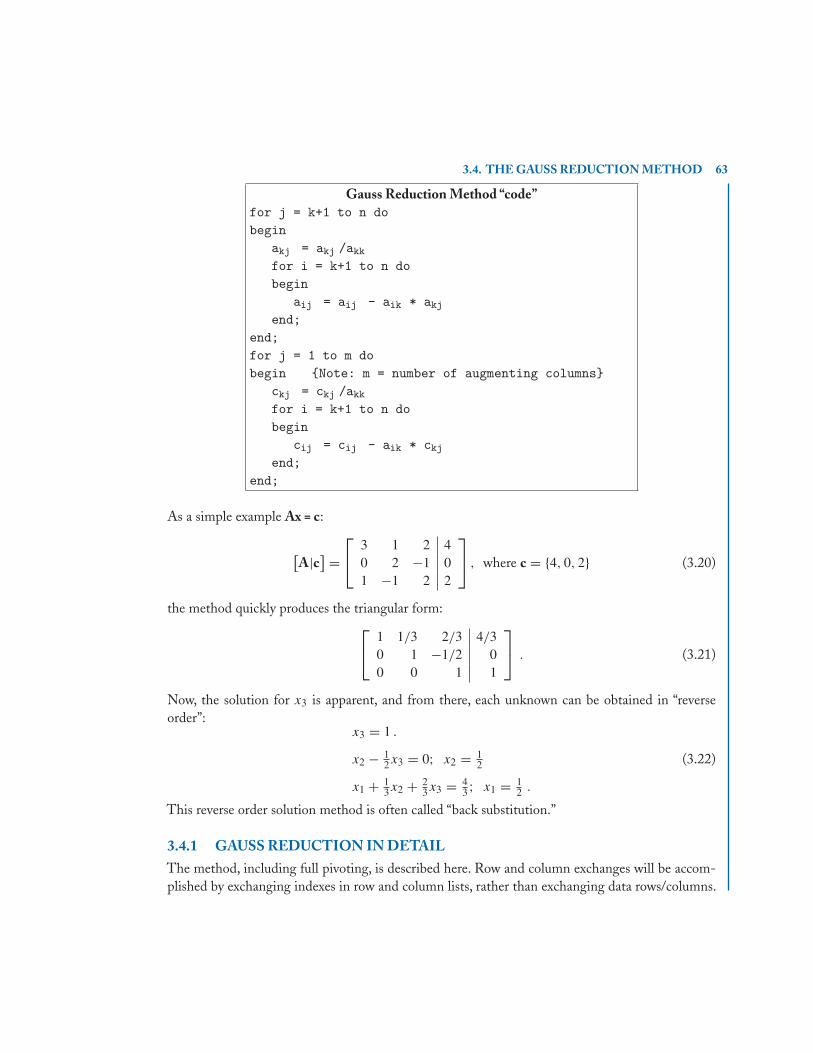
3.4. THE GAUSS REDUCTION METHOD 63
Gauss Reduction Method “code”for j = k+1 to n dobegin
akj = akj /akkfor i = k+1 to n dobegin
aij = aij - aik * akjend;
end;for j = 1 to m dobegin {Note: m = number of augmenting columns}
ckj = ckj /akkfor i = k+1 to n dobegin
cij = cij - aik * ckjend;
end;
As a simple example Ax = c:
[A|c] =
⎡⎣ 3 1 2 4
0 2 −1 01 −1 2 2
⎤⎦ , where c = {4, 0, 2} (3.20)
the method quickly produces the triangular form:⎡⎣ 1 1/3 2/3 4/3
0 1 −1/2 00 0 1 1
⎤⎦ . (3.21)
Now, the solution for x3 is apparent, and from there, each unknown can be obtained in “reverseorder”:
x3 = 1 .
x2 − 12x3 = 0; x2 = 1
2
x1 + 13x2 + 2
3x3 = 43 ; x1 = 1
2 .
(3.22)
This reverse order solution method is often called “back substitution.”
3.4.1 GAUSS REDUCTION IN DETAILThe method, including full pivoting, is described here. Row and column exchanges will be accom-plished by exchanging indexes in row and column lists, rather than exchanging data rows/columns.
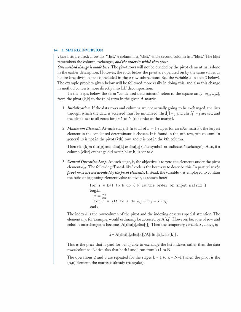
64 3. MATRIX INVERSION
Three lists are used: a row list, “rlist,” a column list, “clist,” and a second column list, “blist.” The blistremembers the column exchanges, and the order in which they occur.One method change is made here: The pivot rows will not be divided by the pivot element, as is donein the earlier description. However, the rows below the pivot are operated on by the same values asbefore (the division step is included in these row subtractions. See the variable x in step 3 below).The example problem given below will be followed more easily in doing this, and also this changein method converts more directly into LU decomposition.
In the steps, below, the term “condensed determinant” refers to the square array |akk , ann|,from the pivot (k,k) to the (n,n) term in the given A matrix.
1. Initialization. If the data rows and columns are not actually going to be exchanged, the liststhrough which the data is accessed must be initialized. rlist[j] = j and clist[j] = j are set, andthe blist is set to all zeros for j = 1 to N (the order of the matrix).
2. Maximum Element. At each stage, k (a total of n − 1 stages for an nXn matrix), the largestelement in the condensed determinant is chosen. It is found in the pth row, qth column. Ingeneral, p is not in the pivot (kth) row, and q is not in the kth column.
Then rlist[k]⇔rlist[p] and clist[k]⇔clist[q] (The symbol ⇔ indicates “exchange”). Also, if acolumn (clist) exchange did occur, blist[k] is set to q.
3. Central Operation Loop. At each stage, k, the objective is to zero the elements under the pivotelement akk .The following “Pascal-like” code is the best way to describe this. In particular, thepivot rows are not divided by the pivot elements. Instead, the variable x is employed to containthe ratio of beginning element value to pivot, as shown here:
for i = k+1 to N do { N is the order of input matrix }begin
x = aik
akk
for j = k+1 to N do aij = aij − x · akj
end;
The index k is the row/column of the pivot and the indexing deserves special attention. Theelement aij , for example, would ordinarily be accessed by A[i,j]. However, because of row andcolumn interchanges it becomes A[rlist[i],clist[j]]. Then the temporary variable x, above, is
x = A[rlist[i],clist[k]]/A[rlist[k],clist[k]] .
This is the price that is paid for being able to exchange the list indexes rather than the datarows/columns. Notice also that both i and j run from k+1 to N.
The operations 2 and 3 are repeated for the stages k = 1 to k = N–1 (when the pivot is the(n,n) element, the matrix is already triangular).
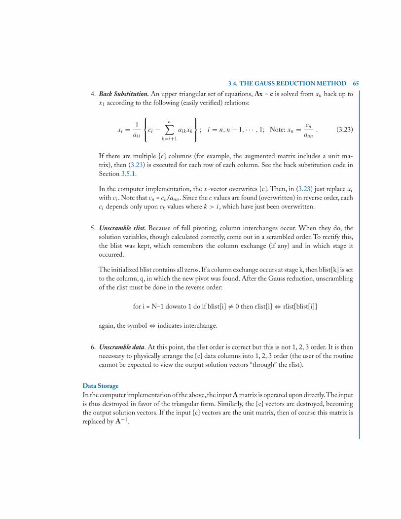
3.4. THE GAUSS REDUCTION METHOD 65
4. Back Substitution. An upper triangular set of equations, Ax = c is solved from xn back up tox1 according to the following (easily verified) relations:
xi = 1
aii
⎧⎨⎩ci −
n∑k=i+1
aikxk
⎫⎬⎭ ; i = n, n − 1, · · · , 1; Note: xn = cn
ann
. (3.23)
If there are multiple {c} columns (for example, the augmented matrix includes a unit ma-trix), then (3.23) is executed for each row of each column. See the back substitution code inSection 3.5.1.
In the computer implementation, the x-vector overwrites {c}. Then, in (3.23) just replace xi
with ci . Note that cn = cn/ann. Since the c values are found (overwritten) in reverse order, eachci depends only upon ck values where k > i, which have just been overwritten.
5. Unscramble rlist. Because of full pivoting, column interchanges occur. When they do, thesolution variables, though calculated correctly, come out in a scrambled order. To rectify this,the blist was kept, which remembers the column exchange (if any) and in which stage itoccurred.
The initialized blist contains all zeros. If a column exchange occurs at stage k, then blist[k] is setto the column, q, in which the new pivot was found. After the Gauss reduction, unscramblingof the rlist must be done in the reverse order:
for i = N–1 downto 1 do if blist[i] �= 0 then rlist[i] ⇔ rlist[blist[i]]
again, the symbol ⇔ indicates interchange.
6. Unscramble data. At this point, the rlist order is correct but this is not 1, 2, 3 order. It is thennecessary to physically arrange the {c} data columns into 1, 2, 3 order (the user of the routinecannot be expected to view the output solution vectors “through” the rlist).
Data StorageIn the computer implementation of the above, the input A matrix is operated upon directly.The inputis thus destroyed in favor of the triangular form. Similarly, the {c} vectors are destroyed, becomingthe output solution vectors. If the input {c} vectors are the unit matrix, then of course this matrix isreplaced by A−1.
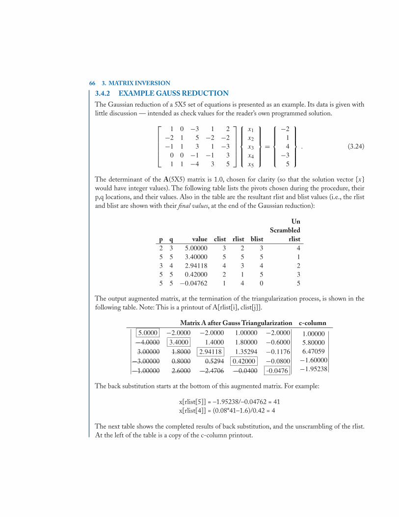
66 3. MATRIX INVERSION
3.4.2 EXAMPLE GAUSS REDUCTIONThe Gaussian reduction of a 5X5 set of equations is presented as an example. Its data is given withlittle discussion — intended as check values for the reader’s own programmed solution.
⎡⎢⎢⎢⎢⎣
1 0 −3 1 2−2 1 5 −2 −2−1 1 3 1 −3
0 0 −1 −1 31 1 −4 3 5
⎤⎥⎥⎥⎥⎦
⎧⎪⎪⎪⎪⎨⎪⎪⎪⎪⎩
x1
x2
x3
x4
x5
⎫⎪⎪⎪⎪⎬⎪⎪⎪⎪⎭
=
⎧⎪⎪⎪⎪⎨⎪⎪⎪⎪⎩
−214
−35
⎫⎪⎪⎪⎪⎬⎪⎪⎪⎪⎭
. (3.24)
The determinant of the A(5X5) matrix is 1.0, chosen for clarity (so that the solution vector {x}would have integer values). The following table lists the pivots chosen during the procedure, theirp,q locations, and their values. Also in the table are the resultant rlist and blist values (i.e., the rlistand blist are shown with their final values, at the end of the Gaussian reduction):
UnScrambled
p q value clist rlist blist rlist2 3 5.00000 3 2 3 45 5 3.40000 5 5 5 13 4 2.94118 4 3 4 25 5 0.42000 2 1 5 35 5 −0.04762 1 4 0 5
The output augmented matrix, at the termination of the triangularization process, is shown in thefollowing table. Note: This is a printout of A[rlist[i], clist[j]].
Matrix A after Gauss Triangularization c-column∣∣∣∣∣∣∣∣∣∣∣
5.0000 −2.0000 −2.0000 1.00000 −2.0000−4.0000 3.4000 1.4000 1.80000 −0.60003.00000 1.8000 2.94118 1.35294 −0.1176
−3.00000 0.8000 0.5294 0.42000 −0.0800
−1.00000 2.6000 −2.4706 −0.0400 -0.0476
∣∣∣∣∣∣∣∣∣∣∣
1.000005.800006.47059
−1.60000−1.95238
∣∣∣∣∣∣∣∣∣∣The back substitution starts at the bottom of this augmented matrix. For example:
x[rlist[5]] = –1.95238/–0.04762 = 41x[rlist[4]] = (0.08*41–1.6)/0.42 = 4
The next table shows the completed results of back substitution, and the unscrambling of the rlist.At the left of the table is a copy of the c-column printout.
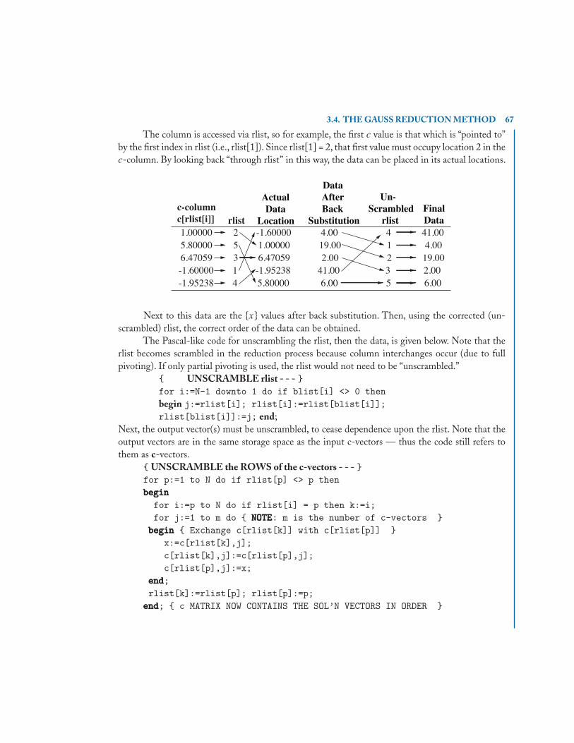
3.4. THE GAUSS REDUCTION METHOD 67
The column is accessed via rlist, so for example, the first c value is that which is “pointed to”by the first index in rlist (i.e., rlist[1]). Since rlist[1] = 2, that first value must occupy location 2 in thec-column. By looking back “through rlist” in this way, the data can be placed in its actual locations.
1.00000 2 -1.60000 4.00 4 41.005.80000 5 1.00000 19.00 1 4.006.47059 3 6.47059 2.00 2 19.00-1.60000 1 -1.95238 41.00 3 2.00-1.95238 4 5.80000 6.00 5 6.00
c-columnc[rlist[i]] rlist
Actual Data
Location
Data After Back
Substitution
Un-Scrambled
rlistFinal Data
Next to this data are the {x} values after back substitution. Then, using the corrected (un-scrambled) rlist, the correct order of the data can be obtained.
The Pascal-like code for unscrambling the rlist, then the data, is given below. Note that therlist becomes scrambled in the reduction process because column interchanges occur (due to fullpivoting). If only partial pivoting is used, the rlist would not need to be “unscrambled.”
{ UNSCRAMBLE rlist - - - }for i:=N-1 downto 1 do if blist[i] <> 0 thenbegin j:=rlist[i]; rlist[i]:=rlist[blist[i]];rlist[blist[i]]:=j; end;
Next, the output vector(s) must be unscrambled, to cease dependence upon the rlist. Note that theoutput vectors are in the same storage space as the input c-vectors — thus the code still refers tothem as c-vectors.
{ UNSCRAMBLE the ROWS of the c-vectors - - - }for p:=1 to N do if rlist[p] <> p thenbeginbeginbegin
for i:=p to N do if rlist[i] = p then k:=i;for j:=1 to m do { NOTENOTENOTE: m is the number of c-vectors }
beginbeginbegin { Exchange c[rlist[k]] with c[rlist[p]] }x:=c[rlist[k],j];c[rlist[k],j]:=c[rlist[p],j];c[rlist[p],j]:=x;
endendend;rlist[k]:=rlist[p]; rlist[p]:=p;
endendend; { c MATRIX NOW CONTAINS THE SOL’N VECTORS IN ORDER }
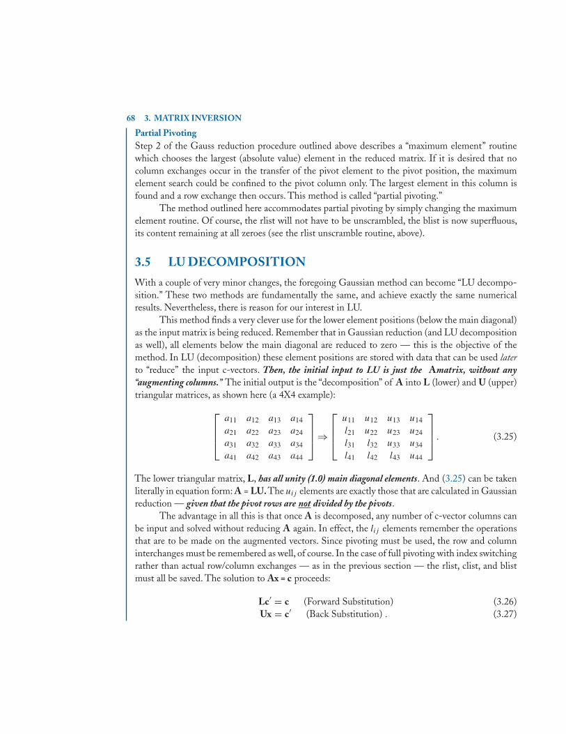
68 3. MATRIX INVERSION
Partial PivotingStep 2 of the Gauss reduction procedure outlined above describes a “maximum element” routinewhich chooses the largest (absolute value) element in the reduced matrix. If it is desired that nocolumn exchanges occur in the transfer of the pivot element to the pivot position, the maximumelement search could be confined to the pivot column only. The largest element in this column isfound and a row exchange then occurs. This method is called “partial pivoting.”
The method outlined here accommodates partial pivoting by simply changing the maximumelement routine. Of course, the rlist will not have to be unscrambled, the blist is now superfluous,its content remaining at all zeroes (see the rlist unscramble routine, above).
3.5 LU DECOMPOSITION
With a couple of very minor changes, the foregoing Gaussian method can become “LU decompo-sition.” These two methods are fundamentally the same, and achieve exactly the same numericalresults. Nevertheless, there is reason for our interest in LU.
This method finds a very clever use for the lower element positions (below the main diagonal)as the input matrix is being reduced. Remember that in Gaussian reduction (and LU decompositionas well), all elements below the main diagonal are reduced to zero — this is the objective of themethod. In LU (decomposition) these element positions are stored with data that can be used laterto “reduce” the input c-vectors. Then, the initial input to LU is just the Amatrix, without any“augmenting columns.” The initial output is the “decomposition” of A into L (lower) and U (upper)triangular matrices, as shown here (a 4X4 example):
⎡⎢⎢⎣
a11 a12 a13 a14
a21 a22 a23 a24
a31 a32 a33 a34
a41 a42 a43 a44
⎤⎥⎥⎦ ⇒
⎡⎢⎢⎣
u11 u12 u13 u14
l21 u22 u23 u24
l31 l32 u33 u34
l41 l42 l43 u44
⎤⎥⎥⎦ . (3.25)
The lower triangular matrix, L, has all unity (1.0) main diagonal elements. And (3.25) can be takenliterally in equation form: A = LU. The uij elements are exactly those that are calculated in Gaussianreduction — given that the pivot rows are not divided by the pivots.
The advantage in all this is that once A is decomposed, any number of c-vector columns canbe input and solved without reducing A again. In effect, the lij elements remember the operationsthat are to be made on the augmented vectors. Since pivoting must be used, the row and columninterchanges must be remembered as well, of course. In the case of full pivoting with index switchingrather than actual row/column exchanges — as in the previous section — the rlist, clist, and blistmust all be saved. The solution to Ax = c proceeds:
Lc′ = c (Forward Substitution) (3.26)Ux = c′ (Back Substitution) . (3.27)
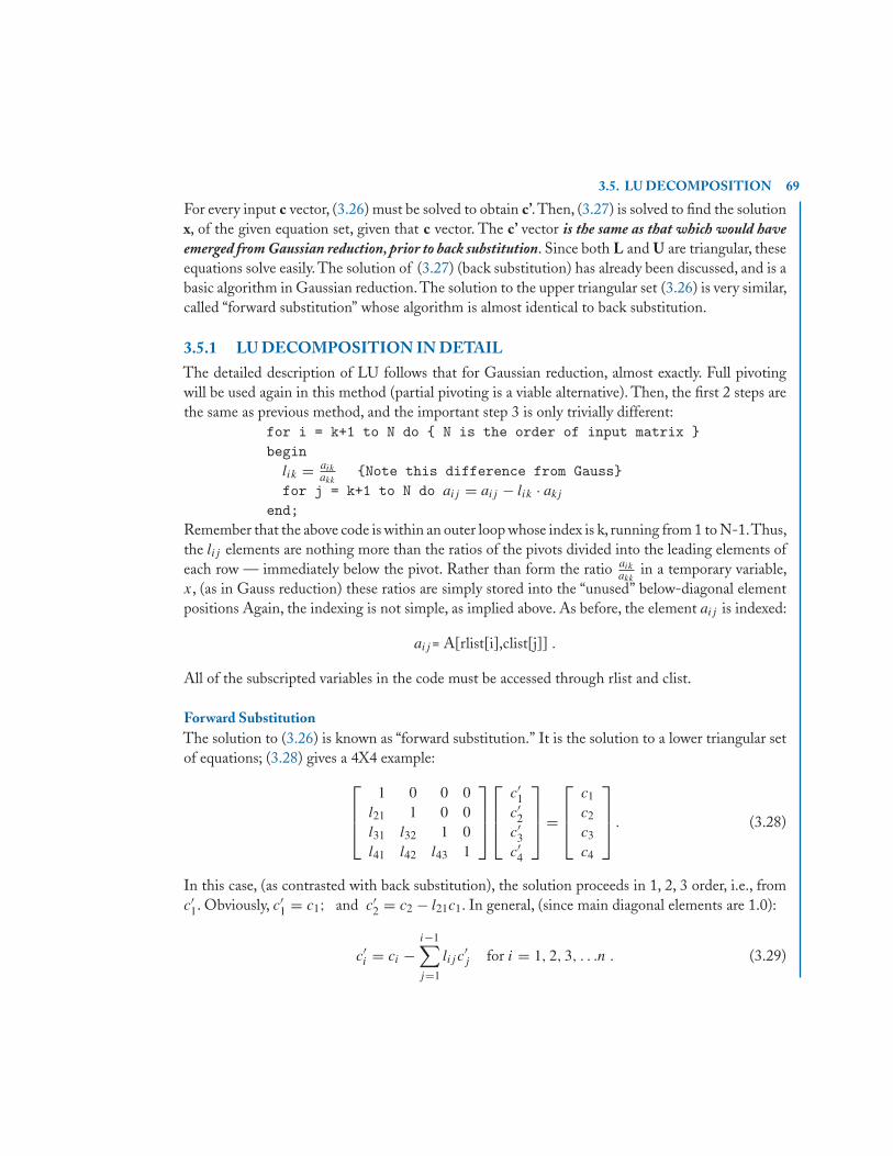
3.5. LU DECOMPOSITION 69
For every input c vector, (3.26) must be solved to obtain c’.Then, (3.27) is solved to find the solutionx, of the given equation set, given that c vector. The c’ vector is the same as that which would haveemerged from Gaussian reduction, prior to back substitution. Since both L and U are triangular, theseequations solve easily. The solution of (3.27) (back substitution) has already been discussed, and is abasic algorithm in Gaussian reduction.The solution to the upper triangular set (3.26) is very similar,called “forward substitution” whose algorithm is almost identical to back substitution.
3.5.1 LU DECOMPOSITION IN DETAILThe detailed description of LU follows that for Gaussian reduction, almost exactly. Full pivotingwill be used again in this method (partial pivoting is a viable alternative). Then, the first 2 steps arethe same as previous method, and the important step 3 is only trivially different:
for i = k+1 to N do { N is the order of input matrix }begin
lik = aik
akk{Note this difference from Gauss}
for j = k+1 to N do aij = aij − lik · akj
end;Remember that the above code is within an outer loop whose index is k, running from 1 to N-1.Thus,the lij elements are nothing more than the ratios of the pivots divided into the leading elements ofeach row — immediately below the pivot. Rather than form the ratio aik
akkin a temporary variable,
x, (as in Gauss reduction) these ratios are simply stored into the “unused” below-diagonal elementpositions Again, the indexing is not simple, as implied above. As before, the element aij is indexed:
aij = A[rlist[i],clist[j]] .
All of the subscripted variables in the code must be accessed through rlist and clist.
Forward SubstitutionThe solution to (3.26) is known as “forward substitution.” It is the solution to a lower triangular setof equations; (3.28) gives a 4X4 example:
⎡⎢⎢⎣
1 0 0 0l21 1 0 0l31 l32 1 0l41 l42 l43 1
⎤⎥⎥⎦⎡⎢⎢⎣
c′1
c′2
c′3
c′4
⎤⎥⎥⎦ =
⎡⎢⎢⎣
c1
c2
c3
c4
⎤⎥⎥⎦ . (3.28)
In this case, (as contrasted with back substitution), the solution proceeds in 1, 2, 3 order, i.e., fromc′
1. Obviously, c′1 = c1; and c′
2 = c2 − l21c1. In general, (since main diagonal elements are 1.0):
c′i = ci −
i−1∑j=1
lij c′j for i = 1, 2, 3, . . .n . (3.29)
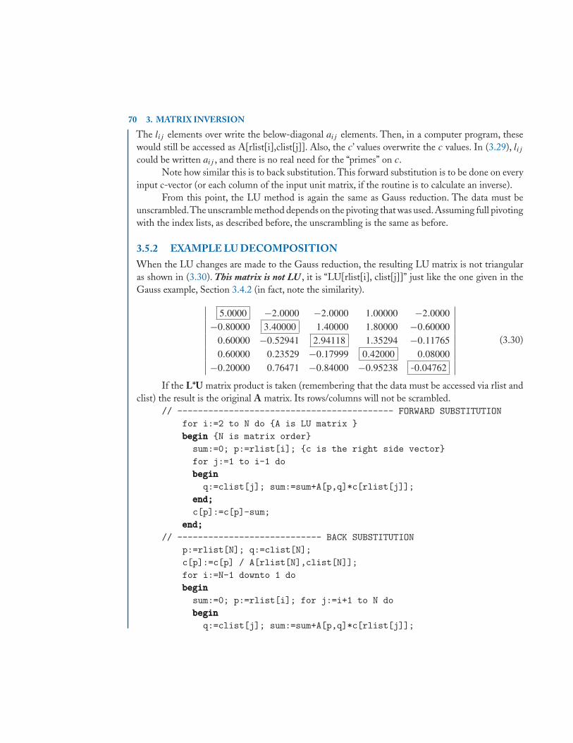
70 3. MATRIX INVERSION
The lij elements over write the below-diagonal aij elements. Then, in a computer program, thesewould still be accessed as A[rlist[i],clist[j]]. Also, the c’ values overwrite the c values. In (3.29), lij
could be written aij , and there is no real need for the “primes” on c.Note how similar this is to back substitution. This forward substitution is to be done on every
input c-vector (or each column of the input unit matrix, if the routine is to calculate an inverse).From this point, the LU method is again the same as Gauss reduction. The data must be
unscrambled.The unscramble method depends on the pivoting that was used.Assuming full pivotingwith the index lists, as described before, the unscrambling is the same as before.
3.5.2 EXAMPLE LU DECOMPOSITIONWhen the LU changes are made to the Gauss reduction, the resulting LU matrix is not triangularas shown in (3.30). This matrix is not LU , it is “LU[rlist[i], clist[j]]” just like the one given in theGauss example, Section 3.4.2 (in fact, note the similarity).
5.0000 −2.0000 −2.0000 1.00000 −2.0000−0.80000 3.40000 1.40000 1.80000 −0.60000
0.60000 −0.52941 2.94118 1.35294 −0.117650.60000 0.23529 −0.17999 0.42000 0.08000
−0.20000 0.76471 −0.84000 −0.95238 -0.04762
(3.30)
If the L*U matrix product is taken (remembering that the data must be accessed via rlist andclist) the result is the original A matrix. Its rows/columns will not be scrambled.
// ------------------------------------------ FORWARD SUBSTITUTIONfor i:=2 to N do {A is LU matrix }beginbeginbegin {N is matrix order}
sum:=0; p:=rlist[i]; {c is the right side vector}for j:=1 to i-1 dobeginbeginbegin
q:=clist[j]; sum:=sum+A[p,q]*c[rlist[j]];end;end;end;c[p]:=c[p]-sum;
end;end;end;// ---------------------------- BACK SUBSTITUTION
p:=rlist[N]; q:=clist[N];c[p]:=c[p] / A[rlist[N],clist[N]];for i:=N-1 downto 1 dobeginbeginbegin
sum:=0; p:=rlist[i]; for j:=i+1 to N dobeginbeginbegin
q:=clist[j]; sum:=sum+A[p,q]*c[rlist[j]];
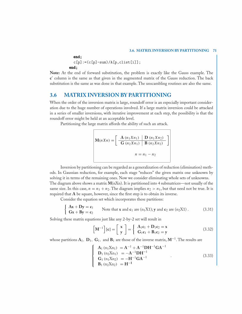
3.6. MATRIX INVERSION BY PARTITIONING 71
end;end;end;c[p]:=(c[p]-sum)/A[p,clist[i]];
end;end;end;Note: At the end of forward substitution, the problem is exactly like the Gauss example. Thec′ column is the same as that given in the augmented matrix of the Gauss reduction. The backsubstitution is the same as was done in that example. The unscambling routines are also the same.
3.6 MATRIX INVERSION BY PARTITIONINGWhen the order of the inversion matrix is large, roundoff error is an especially important consider-ation due to the huge number of operations involved. If a large matrix inversion could be attackedin a series of smaller inversions, with iterative improvement at each step, the possibility is that theroundoff error might be held at an acceptable level.
Partitioning the large matrix affords the ability of such an attack.
M(nXn) =[
A (n1Xn1) D (n1Xn2)
G (n2Xn1) B (n2Xn2)
]
n = n1 − n2
Inversion by partitioning can be regarded as a generalization of reduction (elimination) meth-ods. In Gaussian reduction, for example, each stage “reduces” the given matrix one unknown bysolving it in terms of the remaining ones. Now we consider eliminating whole sets of unknowns.The diagram above shows a matrix M(nXn). It is partitioned into 4 submatrices—not usually of thesame size. In this case, n = n1 + n2. The diagram implies n2 > n1, but that need not be true. It isrequired that A be square, however, since the first step is to obtain its inverse.
Consider the equation set which incorporates these partitions:{Ax + Dy = c1
Gx + By = c2Note that x and c1 are (n1X1); y and c2 are (n2X1) . (3.31)
Solving these matrix equations just like any 2-by-2 set will result in[M−1
][c] =
[xy
]={
A1c1 + D1c2 = xG1c1 + B1c2 = y
(3.32)
whose partitions A1, D1, G1, and B1 are those of the inverse matrix, M−1. The results are⎧⎪⎪⎪⎨⎪⎪⎪⎩
A1 (n1Xn1) = A−1 + A−1DH−1GA−1
D1 (n2Xn1) = −A−1DH−1
G1 (n1Xn2) = −H−1GA−1
B1 (n2Xn2) = H−1
. (3.33)
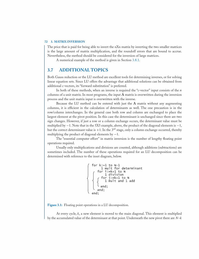
72 3. MATRIX INVERSION
The price that is paid for being able to invert the nXn matrix by inverting the two smaller matricesis the large amount of matrix multiplication, and the roundoff errors that are bound to accrue.Nevertheless, the method should be considered for the inversion of large matrices.
A numerical example of the method is given in Section 3.8.1.
3.7 ADDITIONAL TOPICSBoth Gauss reduction or the LU method are excellent tools for determining inverses, or for solvinglinear equation sets. Since LU offers the advantage that additional solutions can be obtained fromadditional c-vectors, its “forward substitution” is preferred.
In both of these methods, when an inverse is required the “c-vector” input consists of the n
columns of a unit matrix. In most programs, the input A matrix is overwritten during the inversionprocess and the unit matrix input is overwritten with the inverse.
Because the LU method can be entered with just the A matrix without any augmentingcolumns, it is efficient in the calculation of determinants as well. The one precaution is in therow/column interchanges. In the general case both row and column are exchanged to place thelargest element at the pivot position. In this case the determinant is unchanged since there are twosign changes. However, if just a row or a column exchange occurs, the determinant value must bemultiplied by −1. Note that in the 5X5 example, above, the product of the diagonal elements is −1,but the correct determinant value is +1. In the 3rd stage, only a column exchange occurred, therebymultiplying the product of diagonal elements by −1.
The “essential computer effort” in matrix inversion is the number of lengthy floating pointoperations required.
Usually only multiplications and divisions are counted, although additions (subtractions) aresometimes included. The number of these operations required for an LU decomposition can bedetermined with reference to the inset diagram, below.
Figure 3.1: Floating point operations in a LU decomposition.
At every cycle, k, a new element is moved to the main diagonal. This element is multipliedby the accumulated value of the determinant at that point. Underneath the new pivot there are N–k
3.7. ADDITIONAL TOPICS 73
elements which must be divided by the pivot (to determine the lij elements). Adjacent to each ofthese are N–k elements, aij , from whom are subtracted a product. Then, for the kth execution of theouter loop there are N–k divisions, and (N–k)2 multiplications and subtractions.The multiplicationfor the determinant value is neglected since it is not an essential part of the method. Then, thenumber of divisions:
div =N−1∑k=1
(N − k) = 12N(N − 1) .
The number of multiplications and subtractions are
mult =N−1∑k=1
(N − k)2 = 16N(N − 1)(2N − 1) .
The sum of divisions plus multiplications
12N(N − 1) + 1
6N(N − 1)(2N − 1) = 13N(N2 − 1) .
In a matrix inversion there are N “c-vectors” most of whose elements are zero. However, it is veryunusual for the program to take advantage of this fact. Therefore, we will consider the general casein which N c-vectors are input. In this case, entirely similar reasoning leads to
Forward Substitution ops = 12N2(N − 1)
Backward Substitution ops = 12N2(N + 1) .
The total inversion process, then, requires N3 operations. With the speed and precision of moderncomputers this numbers is a problem only when the matrix is very large. Although the inversionof these very large systems is outside the scope of this work, several of the following paragraphsspeak to the problem by discussing column normalization, improving the inverse, and inversion byorthogonalization.
3.7.1 COLUMN NORMALIZATIONIf the determinant of the matrix is “ill-conditioned,” the inversion process may accumulate error oreven fail. In Section 2.7 of Chapter 2 it was shown that a determinant value, |A|, is geometricallyrelated to the n-dimensional volume enclosed within the column vectors of A. If one or more ofthese vectors is disproportionately small, the determinant value will be small. The condition is easilyspotted, and easily fixed. Simply write:
Ax = c ⇒ a1x1 + a2x2 + a3x3 + · · · = c
Now, change the variables, xj = αjyj and set the α value such that its vector, a, is normalized tounit length.
74 3. MATRIX INVERSION
The other source of problem is determinant “skew.” In the worst case one or more of thecolumn vectors is a linear combination of the others—the matrix is singular, no inverse exists. Inless severe cases the input matrix may be resolved into the product of an orthogonal matrix and atriangular one; see Section 3.7.4.
3.7.2 IMPROVING THE INVERSEMatrix inversion is characterized by a large number of simple arithmetic operations (in fact, onthe order of N3 of them). It is not unusual for the inverse process to lose precision due to theaccumulation of roundoff error. The accumulation is greater the larger the matrix, of course, and isparticularly troublesome when the matrix is nearly singular.
In general, the input matrix is not known exactly, with element values the result of measure-ment. Then, an exact inverse is rarely required. Instead, we invoke a clever iterative process whichcan usually restore all the precision that is meaningful to the problem.
The matrix equation AX = I defines X as A−1. Each column of I is the product of Ax, wherex is the corresponding column within X. For simplicity, then, consider Ax = b, where the vector b isany one of the vectors in I. This equation set is to be solved for x, using LU decomposition followedby forward and back substitution.
Of course the set has an exact solution, x, but the accumulation of roundoff error produces asomewhat different vector, x0 = x + �x. The (hopefully small) �x is the departure from the exactsolution, and it produces a “residual” vector, �b. That is:
A(x + �x) = b + �b, and since Ax = b (3.34)A�x = �b . (3.35)
Now, �b is simply Ax0 – b, and b is known — it’s one of the columns of I. Then the iterative processis:
1. Save the input A matrix. Use LU and forward, back substitution → x0.
2. Multiply Ax0 and subtract b → �b. If the elements of �b are small enough, then stop, else:
3. Use forward back substitution with �b as input → �x.
4. Subtract �x from x0 → Defines a new x0.
5. Go back to step 2.
When a stop occurs at step 2, the �b is within the required precision and the x vector is the improvedsolution.
Especially note that step 3 does not involve LU decomposition. The LU matrix already exists, havingbeen produced in step 1. Remember that this is the primary advantage of LU, compared to Gaussreduction — the ability to input any number of vectors, after the input matrix has been decomposed.
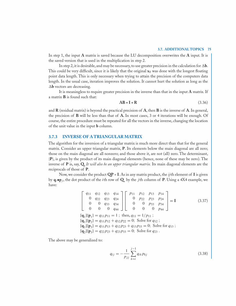
3.7. ADDITIONAL TOPICS 75
In step 1, the input A matrix is saved because the LU decomposition overwrites the A input. It isthe saved version that is used in the multiplication in step 2.
In step 2, it is desirable, and may be necessary, to use greater precision in the calculation for �b.This could be very difficult, since it is likely that the original x0 was done with the longest floatingpoint data length. This is only necessary when trying to attain the precision of the computers datalength. In the usual case, iteration improves the solution. It cannot hurt the solution as long as the�b vectors are decreasing.
It is meaningless to require greater precision in the inverse than that in the input A matrix. Ifa matrix B is found such that:
AB = I + R (3.36)
and R (residual matrix) is beyond the practical precision of A, then B is the inverse of A. In general,the precision of B will be less than that of A. In most cases, 3 or 4 iterations will be enough. Ofcourse, the entire procedure must be repeated for all the vectors in the inverse, changing the locationof the unit value in the input b column.
3.7.3 INVERSE OF A TRIANGULAR MATRIXThe algorithm for the inversion of a triangular matrix is much more direct than that for the generalmatrix. Consider an upper triangular matrix, P. Its elements below the main diagonal are all zero;those on the main diagonal are all nonzero; and those above it, are not (all) zero. The determinant,|P|, is given by the product of its main diagonal elements (hence, none of these may be zero). Theinverse of P is, say, Q. It will also be an upper triangular matrix. Its main diagonal elements are thereciprocals of those of P.
Now, we consider the product QP = I. As in any matrix product, the ijth element of I is givenby qi•pj , the dot product of the ith row of Q by the j th column of P. Using a 4X4 example, wehave: ⎡
⎢⎢⎣q11 q12 q13 q14
0 q22 q23 q24
0 0 q33 q34
0 0 0 q44
⎤⎥⎥⎦⎡⎢⎢⎣
p11 p12 p13 p14
0 p22 p23 p24
0 0 p33 p34
0 0 0 p44
⎤⎥⎥⎦ = I (3.37)
[q1]{p1} = q11p11 = 1 ; then, q11 = 1/p11 ;[q1]{p2} = q11p12 + q12p22 = 0; Solve for q12 ;[q1]{p3} = q11p13 + q12p23 + q13p33 = 0; Solve for q13 ;[q2]{p3} = q22p23 + q23p33 = 0; Solve for q23 .
The above may be generalized to:
qij = − 1
pjj
j−1∑k=i
qikpkj (3.38)
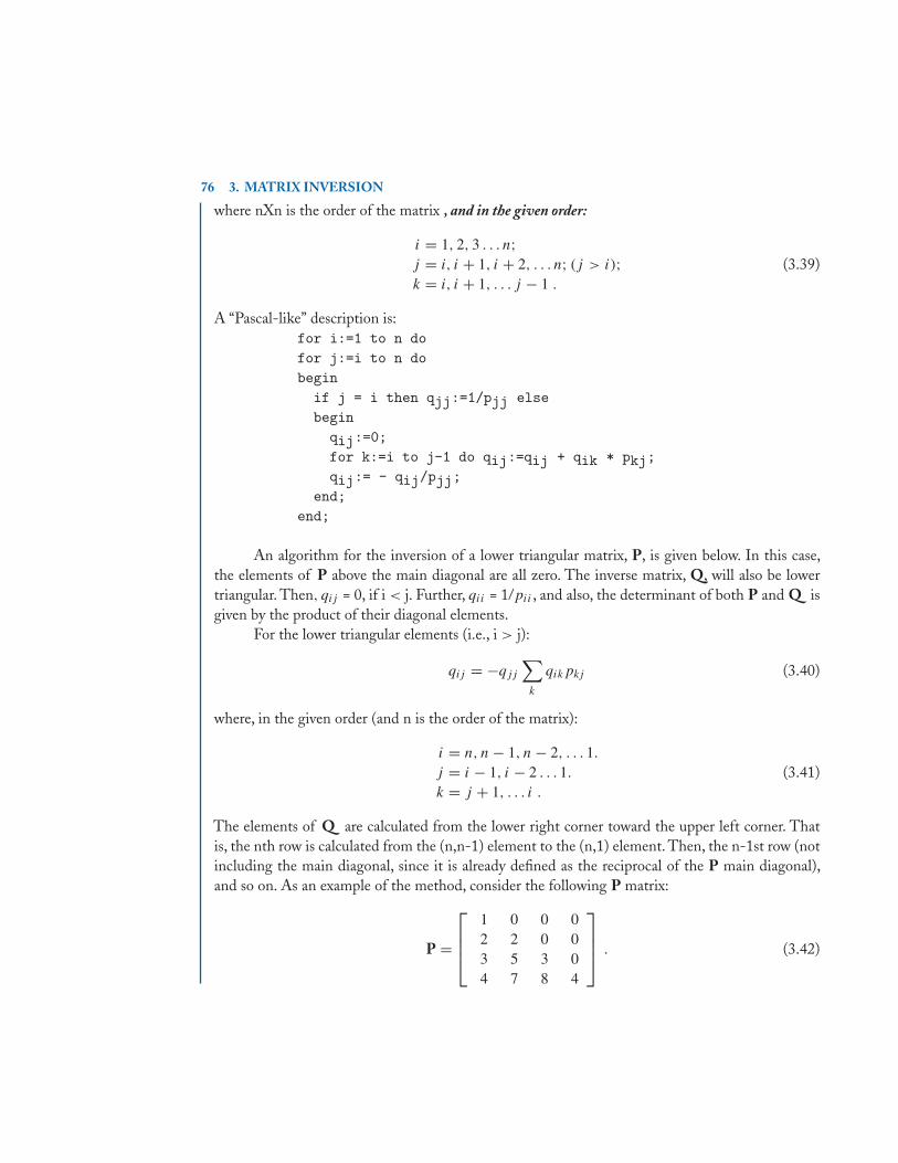
76 3. MATRIX INVERSION
where nXn is the order of the matrix , and in the given order:
i = 1, 2, 3 . . . n;j = i, i + 1, i + 2, . . . n; (j > i); (3.39)k = i, i + 1, . . . j − 1 .
A “Pascal-like” description is:for i:=1 to n dofor j:=i to n dobeginif j = i then qjj:=1/pjj elsebeginqij:=0;for k:=i to j-1 do qij:=qij + qik * pkj;qij:= - qij/pjj;
end;end;
An algorithm for the inversion of a lower triangular matrix, P, is given below. In this case,the elements of P above the main diagonal are all zero. The inverse matrix, Q, will also be lowertriangular. Then, qij = 0, if i < j. Further, qii = 1/pii , and also, the determinant of both P and Q isgiven by the product of their diagonal elements.
For the lower triangular elements (i.e., i > j):
qij = −qjj
∑k
qikpkj (3.40)
where, in the given order (and n is the order of the matrix):
i = n, n − 1, n − 2, . . . 1.
j = i − 1, i − 2 . . . 1. (3.41)k = j + 1, . . . i .
The elements of Q are calculated from the lower right corner toward the upper left corner. Thatis, the nth row is calculated from the (n,n-1) element to the (n,1) element. Then, the n-1st row (notincluding the main diagonal, since it is already defined as the reciprocal of the P main diagonal),and so on. As an example of the method, consider the following P matrix:
P =
⎡⎢⎢⎣
1 0 0 02 2 0 03 5 3 04 7 8 4
⎤⎥⎥⎦ . (3.42)
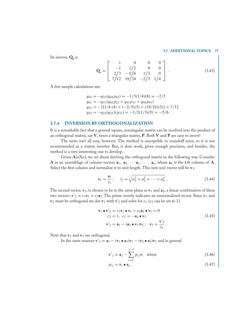
3.7. ADDITIONAL TOPICS 77
Its inverse, Q, is:
Q =
⎡⎢⎢⎣
1 0 0 0−1 1
/2 0 0
2/
3 −5/
6 1/
3 07/
12 19/
24 −2/
3 1/
4
⎤⎥⎥⎦ . (3.43)
A few sample calculations are:
q43 = −q33(q44p43) = −1/3(1/4)(8) = −2/3q41 = −q11(q42p21 + q43p31 + q44p41)
q41 = −1[1/4 (4) + (−2/3)(3) + (19/24)(2)] = 7/12q32 = −q22(q33)(p32) = −1/2(1/3)(5) = −5/6 .
3.7.4 INVERSION BY ORTHOGONALIZATIONIt is a remarkable fact that a general square, nonsingular matrix can be resolved into the product ofan orthogonal matrix, say V, times a triangular matrix, P. Both V and P are easy to invert!
The news isn’t all rosy, however. The method is susceptible to roundoff error, so it is notrecommended as a matrix inverter. But, it does work, given enough precision, and besides, themethod is a very interesting one to develop.
Given A(nXn), we set about deriving the orthogonal matrix in the following way. ConsiderA as an assemblage of column vectors a1, a2, · · · ak, · · · , an, where ak is the kth column of A.Select the first column and normalize it to unit length. This new unit vector will be v1:
v1 = a1
l1; l1 =
√a2
1 + a22 + · · · + a2
n . (3.44)
The second vector, v2, is chosen to be in the same plane as v1 and a2, a linear combination of thesetwo vectors: v ′
2 = c1v1 + c2a2. The prime merely indicates an unnormalized vector. Since v1 andv2 must be orthogonal we dot v1 with v′
2 and solve for c1 (c2 can be set to 1).
v1 • v ′2 = c1v1 • v1 + c2a2 • v1 = 0
c2 = 1, c1 = −a2 • v1 (3.45)
v ′2 = a2 − (a2 • v1)v1 ; v2 = v ′
2
l2.
Note that v1 and v2 are orthogonal.In the same manner v ′
3 = a3 − (v1 • a3)v1 − (v2 • a3)v2 and in general
v ′j = aj −
j−1∑i=1
pij vi where (3.46)
pij = vi • aj . (3.47)
78 3. MATRIX INVERSION
The pij factors can be arranged into an upper triangular matrix, with the main diagonal elementsbeing the normalization lengths of the vectors, lj . Note that the j th column of P provides the pij
factors in (3.46).Further, solving (3.46) for aj
aj = pjj vj + p(j−1)j vj−1 + · · · + p1j v1
pjj = lj =√
v21j + v2
2j + · · · + v2nj .
That is:
A = VP . (3.48)
The inversion of A is now a relatively simple matter. The triangular Q = P−1 has been discussedearlier, and the inverse of V is obtained by transposition (V−1 = V t ). Then
A−1 = QV t . (3.49)
3.7.5 INVERSION OF A COMPLEX MATRIXThe Gauss reduction method, and any other method that will successfully invert a real matrix, willwork equally well on a matrix whose elements are complex — given that the routines used supportcomplex arithmetic. Some minor adjustments must be made. For example, the routine which choosesthe largest element now must be made to determine the absolute value of a complex number.
Complex arithmetic can be difficult to do if the compiler itself does not recognize the complextype. Also, the need for inversion of a complex matrix may not arise often enough. So, whatever thereason, it may be required to invert the complex matrix using only real arithmetic, and real numbers:Find a complex matrix B such that AB = I, where A is complex. Then:
(Ar + jAi )(Br + jBi ) = I ; j2 = −1 . (3.50)
Equating real (subscript, r) and imaginary (subscript, i) parts:
ArBr − AiBi = I and ArBi = −AiBr .
Then, assuming that Ar has an inverse, Bi = −A−1r AiBr and (Ar + AiA−1
r Ai )Br = I.And the elements of the complex matrix Br + jBi are
{Br = (Ar + AiA−1
r Ai )−1
Bi = −A−1r AiBr .
(3.51)
Notice that the increased difficulty of complex numbers cannot be avoided. Although just twomatrices must be inverted, both just nXn, there is a lot of matrix multiplication involved.
3.8. EXAMPLES 79
3.8 EXAMPLES3.8.1 INVERSION USING PARTITIONSThis example intends to simulate the inversion of a large matrix. For reasons of clarity and lack ofspace, this “large” matrix, M, is only 8X8. Its inversion will be affected by inverting no larger than a3X3 array. The process is straightforward, but the “bookkeeping” becomes cumbersome. To begin,M is partitioned as shown, with a 3X3 in the upper left.∥∥∥∥∥∥∥∥∥∥∥∥∥∥∥∥∥
1.00 −2.00 3.00 4.00 0.00 1.00 0.00 0.003.00 −1.00 2.00 5.00 −2.00 −1.00 1.00 0.002.00 4.00 −5.00 1.00 −1.00 2.00 3.00 1.004.00 2.00 −1.00 3.00 0.00 3.00 −2.00 0.00
−2.00 0.00 2.00 −2.00 5.00 1.00 −1.00 1.003.00 1.00 3.00 4.00 2.00 1.00 0.00 −4.001.00 3.00 0.00 −1.00 −2.00 0.00 2.00 0.000.00 −1.00 −1.00 2.00 4.00 −2.00 1.00 2.00
∥∥∥∥∥∥∥∥∥∥∥∥∥∥∥∥∥The four partitions of M are named according to the set of Equations in (3.31):
[A(3x3) D(3x5)
G(5x3) B(5x5)
] [xy
]=[
c1
c2
]= Ax + Dy = c1
Gx + By = c2.
If A(3X3) is inverted the vector, x, can be solved for in terms of the remaining unknowns:
x = A−1(c1 − Dy)
A =∥∥∥∥∥∥
1.00 −2.00 3.003.00 −1.00 2.002.00 4.00 −5.00
∥∥∥∥∥∥ A−1 =∥∥∥∥∥∥
−3.00 2.00 −1.0019.00 −11.00 7.0014.00 −8.00 5.00
∥∥∥∥∥∥Plugging the x value back into the second equation, then solving for y, yields:
(B − GA−1D)y = c2 − GA−1c1
Hy = c2 − GA−1c1; where H=B − GA−1D .
Note that, with A−1 known, H is known — and it has the dimensions of B(5X5).
H =
∥∥∥∥∥∥∥∥∥∥
−20.00 −7.00 −25.00 −11.00 −5.00−50.00 −23.00 −77.00 −17.00 −11.00−78.00 −37.00 −118.00 −28.00 −23.00−82.00 −44.00 −125.00 −27.00 −20.00
51.00 30.00 74.00 18.00 14.00
∥∥∥∥∥∥∥∥∥∥
80 3. MATRIX INVERSION
It was a coincidence that A−1 has an integer inverse. Because of this coincidence, H is also an integermatrix. H−1 will surely not be “so lucky,” and in order to proceed, we must have H−1. Since thelargest array that can be inverted is 3X3, H must be partitioned — again with a 3X3 in the upperleft position.
The partitions of H will be named A2, D2, G2, and B2, occupying the same positions as thosein the original matrix, M. Proceeding as before:
A2(3x3)w + D2(3x2)z = d1; w = A−12 (d1−D2z)
G2(2x3)w + B2(2x2)z = d2
A2 =∥∥∥∥∥∥
−20.00 −7.00 −25.00−50.00 −23.00 −77.00−78.00 −37.00 −118.00
∥∥∥∥∥∥ A−12 =
∥∥∥∥∥∥−0.2419 0.1774 −0.0645
0.1900 0.7348 −0.51970.1004 −0.3477 0.1971
∥∥∥∥∥∥As before, H2 = (B2 − G2A−1
2 D2), which can now be written because A−12 is known. This time,
H2 will be 2X2, the same dimensions as B2, and will be easy to invert.
H2 H−12∥∥∥∥ 1.6129 17.9355
−2.3907 −21.8244
∥∥∥∥∥∥∥∥ −2.8427 −2.3361
0.3114 0.2101
∥∥∥∥The cumbersome part is that H−1 must be found, which requires a complete solution to the aboveequation set
w = A−12 (d1 − D2z)
z = H−12 (d2 − G2A−1
2 d1).
The value for z must now be plugged back into the expression for w. With some algebra, andrearrangement, the results are like those given in Equations (3.33):
[wz
]=[
H−1] [
d] =
[wz
]=[
A−12 + A−1
2 D2H2G2A−12 −A−1
2 D2H−12
−H−12 G2A−1
2 H−12
][d1
d2
].
This equation defines H−1. Since A−12 and H−1
2 are known, each of the 4 partitions of H−1 can becalculated — for example, its upper left 3X3 is A−1
2 + A−12 D2H−1
2 G2A−12 . See M−1, below.
With H−1 known, using the format of Equation (3.33) M−1 becomes:
M−1 =
∥∥∥∥∥∥∥∥∥∥∥∥∥∥∥∥
−6.0672 8.2063 2.8721 −1.7526 5.2418 −0.1438 −5.3707 −4.34454.7815 −6.6349 −2.4435 1.6097 −4.241 0.1438 4.6564 3.63030.1513 −0.0476 −0.1289 0.0266 0.0392 −0.0098 0.2507 0.02524.4118 −5.8889 −2.0915 1.3595 −3.8562 0.1307 3.8954 3.2353
−1.0840 1.3968 0.5345 −0.3296 0.9967 0.0425 −0.9911 −0.6807−1.4706 2.2222 0.9935 −0.5458 1.5817 −0.0621 −1.6503 −1.4118−3.0168 4.3016 1.7180 −1.1881 2.8105 −0.0359 −2.8427 −2.3361
0.2605 −0.1746 −0.1293 0.1662 −0.0621 −0.1928 0.3114 0.2101
∥∥∥∥∥∥∥∥∥∥∥∥∥∥∥∥
3.9. EXERCISES 81
For example, the lower right 5X5 of M−1 is B1 = H−1. In turn, its lower right 2X2 is H−12 as
written above.If the inverse of M is not required, just the solution to the equation set (3.31), many of the
tedious matrix operations can be avoided.
y = H−1(c2 − GA−1c1)
x = A−1(c1 − Dy)
The solution, above, does require that both A and H must be inverted. However, when this is done,fewer operations remain, and these equations can be solved using “matrix-times-vector” operationsrather than “matrix-times-matrix”. The savings are considerable.
As this example indicates, when the matrix B (and consequently, H1) is still too large to beinverted directly, additional “partitioning” is required until that lower right matrix is within the rangeto be inverted—possibly a lengthy process. But, the final result will retain greater precision than adirect approach.
3.9 EXERCISES
3.1. Given the matrix, A, below, determine Q such that the product QA produces zero elementvalues in the first column of A, except, a11.
What is the determinant value, |A|?
A =⎡⎣ 1 3 −1
3 11 12 6 −1
⎤⎦.
3.2. With the A given in problem 1, determine the solution to Ax = c = {4, 12, 7}. Note that {c}is a column vector.
3.3. Find the inverse of the complex matrix A =⎡⎣ 1 + j0 1 + j2 1 + j8
0 + j1 −1 + j1 −6 + j31 + j1 0 + j5 −8 + j15
⎤⎦.
3.4. Find the inverse of the complex matrix A = Ar + jAi
Ar =⎡⎣ 1 −1 0
0 0 02 0 1
⎤⎦ and Ai =
⎡⎣ 1 −2 3
3 −1 22 4 −5
⎤⎦ .
3.5. Given the equations Ax = c, and A−1 = B. If two columns in A are exchanged, how is thesolution, x, affected? How is B affected?

82 3. MATRIX INVERSION
3.6. Perform an LU decomposition on the 5X5 matrix in Section 3.4.2. Do not use pivoting.Show that L*U does not equal the input S matrix.
3.7. Using the result from exercise 3.6, solve the example problem using the same right-sidec-vector from Equation (3.24).
83
C H A P T E R 4
Linear Simultaneous EquationSets
4.1 INTRODUCTIONThis chapter turns to an interpretation of the solution to linear equation sets, using a geometricapproach and insight. We will look at an equation set in several different (and perhaps new) ways,and consider the solvability and compatibility of an equation set. Most of the mechanics of solutionhave already been discussed. This chapter intends to be largely conceptual.
Many applications in mechanics, dynamics, and electric circuits depend on the insights gained,and presented here.
We begin by defining the equation set Ax = b as “nonhomogeneous” because the b vector isassumed to be nonzero. Associated with this set is the “homogeneous” set, Ax = 0; the same set, butwith the b vector replaced by the zero vector. In the event that matrix A is nonsingular, and has aninverse, the homogeneous set plays no part. But, when A is singular, we will find interest in both Ax= 0, and in A′ x = 0 (the transposed homogeneous set).
4.2 VECTORS AND VECTOR SETSIn order to gain greater insight into its solution, the equation set will be interpreted as a “vectortransformation.” The equation Ax = y “transforms” the columns of A(nXm) into the vector y.Alternatively, y is “synthesized” as a linear vector sum of the column vectors of A.
Ax = y =
⎧⎪⎪⎪⎨⎪⎪⎪⎩
a11
a21...
an1
⎫⎪⎪⎪⎬⎪⎪⎪⎭
x1 +
⎧⎪⎪⎪⎨⎪⎪⎪⎩
a12
a22...
an2
⎫⎪⎪⎪⎬⎪⎪⎪⎭
x2 + · · · +
⎧⎪⎪⎪⎨⎪⎪⎪⎩
a1m
a2m
...
anm
⎫⎪⎪⎪⎬⎪⎪⎪⎭
xm =
⎧⎪⎪⎪⎨⎪⎪⎪⎩
y1
y2...
yn
⎫⎪⎪⎪⎬⎪⎪⎪⎭
, or: (4.1)
= a1x1 + a2x2 + · · · + amxm = y . (4.2)
In this quite general example, A is (nXm); there are m vectors (the columns of A), each with n
coordinates (dimensions — the rows of A). It is often instructive to draw the same vector pictureof the transposed matrix, i.e., A′, whose n column vectors are the rows of A.
To begin, the discussion of vectors in Chapter 1 is reviewed and enlarged upon in the para-graphs, below.
84 4. LINEAR SIMULTANEOUS EQUATION SETS
In two dimensions, a vector, v, is described as {vx ,vy}, where the subscripts “x” and “y” referto unit vectors in a rectangular coordinate set. These unit vectors could be written as {1,0} and {0,1},showing both their orthogonality and their unit length. vx and vy are the components of v alongthe coordinate axes. Extension to three dimensions is simply: v = {vx , vy , vz}, and in either 2 or 3dimensions, it is convenient to use subscripted letters (e.g., “x,” “y,” and “z”) to refer to the unitvectors (the coordinate axes).
The two and three-dimensional cases are familiar, and easily visualized. But, in generalizingto greater than 3 dimensions, visualization is lost. For this reason, the plan will be to view the variousconcepts in the 2 and 3 dimensional cases; then simply extend the reasoning into n-dimensions. Forexample, the definition of a vector:
v = {vx, vy, vz} in three dimensions (4.3)v = {v1, v2, . . . vn} in “n” dimensions (4.4)
is extended to n-dimensions with only a relatively minor change in notation: The coordinate axesare now given numbers, rather than “x, y, z, . .” letters. But these n coordinate axes are still perceivedas rectangular axes, in an “n dimensional space,” and the values, vj are the components of v alongthese axes. In fact, the component vj is defined as the product of the (n-dimensional) length of vmultiplied by the cosine of the angle between v and the j th coordinate axis (i.e., the concept of the“direction cosine,” in n dimensions).
If v is composed of real components, its length is defined as
|v| = sqrt(v21 + v2
2 + · · · + v2n) =
√v2
1 + v22 + · · · + v2
n (4.5)
|v| = sqrt(v•v) = sqrt(v′v) . (4.6)
In (4.6), the notation (v•v) and (v′v) or (vt v) denote the dot product of v into itself, in n dimensions(“n-space”). In general, the dot product of two vectors, u•v, is simply the sum of products of therespective components of the vectors. Equivalently, this (scalar) dot product can be expressed as theproduct of their magnitudes, multiplied by the cosine of the angle between them. Also, two (nonzero)vectors are said to be “orthogonal” in n dimensions if their dot product is zero:
v′u = vt u = (v1u1 + v2u2 + · · · + vnun) = 0 . (4.7)
A vector whose length, |v|, is unity is called a “unit vector.”If the vectors consist of complex numbers, the definitions must be modified. For this purpose,
a new notation is introduced: If c = a + jb is a complex number, its “complex conjugate” (i.e., thenumber a – jb) is denoted c.
Then the length of a complex vector, v, is |v| = sqrt(v•v) = sqrt(v′v). Similarly, the “Hermitian”scalar product between two complex vectors, u and v, is u • v (which is generally complex, and notequal to v • u).
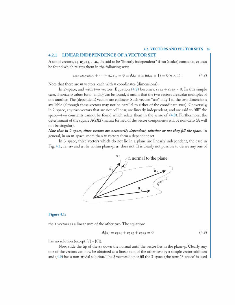
4.2. VECTORS AND VECTOR SETS 85
4.2.1 LINEAR INDEPENDENCE OF A VECTOR SETA set of vectors, a1, a2, a3, …am, is said to be “linearly independent” if no (scalar) constants, ck , canbe found which relates them in the following way:
a1c1a2c2a3c3 + · · · + amcm = 0 ≡ A(n × m)c(m × 1) = 0(n × 1) . (4.8)
Note that there are m vectors, each with n coordinates (dimensions).In 2-space, and with two vectors, Equation (4.8) becomes: c1a1 + c2a2 = 0. In this simple
case, if nonzero values for c1 and c2 can be found, it means that the two vectors are scalar multiples ofone another. The (dependent) vectors are collinear. Such vectors “use” only 1 of the two dimensionsavailable (although these vectors may not be parallel to either of the coordinate axes). Conversely,in 2-space, any two vectors that are not collinear, are linearly independent, and are said to “fill” thespace—two constants cannot be found which relate them in the sense of (4.8). Furthermore, thedeterminant of the square A(2X2) matrix formed of the vector components will be non-zero (A willnot be singular).Note that in 2-space, three vectors are necessarily dependent, whether or not they fill the space. Ingeneral, in an m-space, more than m vectors form a dependent set.
In 3-space, three vectors which do not lie in a plane are linearly independent, the case inFig. 4.1, i.e., a2 and a3 lie within plane-p, a1 does not. It is clearly not possible to derive any one of
Figure 4.1:
the a vectors as a linear sum of the other two. The equation:
A{c} = c1a1 + c2a2 + c3a3 = 0 (4.9)
has no solution (except {c} = {0}).Now, slide the tip of the a1 down the normal until the vector lies in the plane-p. Clearly, any
one of the vectors can now be obtained as a linear sum of the other two by a simple vector additionand (4.9) has a non-trivial solution. The 3 vectors do not fill the 3-space (the term “3-space” is used
86 4. LINEAR SIMULTANEOUS EQUATION SETS
to describe a 3 dimensioanl space. Then, the term “n-space” will refer to a space of n dimensions).With all three vectors in plane-p it is possible to find a fourth vector orthogonal to all three; forexample, the vector n. In general, this circumstance is determined by the existence of a non-trivialsolution to the transposed set,
A′{z} = 0. A′(mXn)z(nX1 = 0(mX1) . (4.10)
The original m vectors are row vectors in A′. If non-trivial z vectors can be found, they areorthogonal to the original set.
Summarizing: the linear (in)dependence of the m vectors in n-space is determined by inves-tigating the possible (non-trival) solutions of equations (4.8) and (4.10). Gauss-Jordan reduction(Section 3.3) is often used in this investigation.
4.2.2 RANK OF A VECTOR SETThe rank of a vector set, A(mXn), is equal to the order of the largest nonvanishing determinantthat can be formed from the matrix A(nXm); and the largest non-vanishing determinant cannot begreater then the smaller of n and m.
In the event that m < n (more dimensions than vectors), and the rank is r < m, the set isdependent and there will be m − r solutions to the equation set (4.8). If r = m then the vector setis independent, and (4.8) has only the trivial solution. This is also true for the “square” case, m = n.
If m > n, the rank of A cannot be greater than n. Necessarily, the m vectors are dependent,and non-trivial solutions will be found for (4.8). Again, the rank could be less than n, in which casethe (many) m vectors still do not fill the n-space.
An obvious example is the A(4X3), shown below, with three 4-dimensional unit vectors.Clearly, the three vectors are independent, although there are only 3 vectors, and the 4-space is notfilled. Because the 4-space is not filled, there must be a vector orthogonal to all the 3 (unit) vectorsshown — one independent solution to A′x = 0. Clearly, that solution is the fourth unit vector. The“rank” of A is 3 — the size of the largest non-zero determinant that can be formed from the elementsof the vectors. ⎡
⎢⎢⎣1 0 00 1 00 0 10 0 0
⎤⎥⎥⎦ .
Also, note that given a y vector: Ax = {y1, y2, y3, 0} (which, obviously, lies in the samesubspace), the solution to Ax = y is x = {y1, y2, y3}. But, if y has y4 �= 0, the set has no solution.
Not quite so obvious is the next example, again 3 vectors, in 4-space.⎡⎢⎢⎣
2 −5 53 −3 61 2 1
−1 −8 1
⎤⎥⎥⎦ .
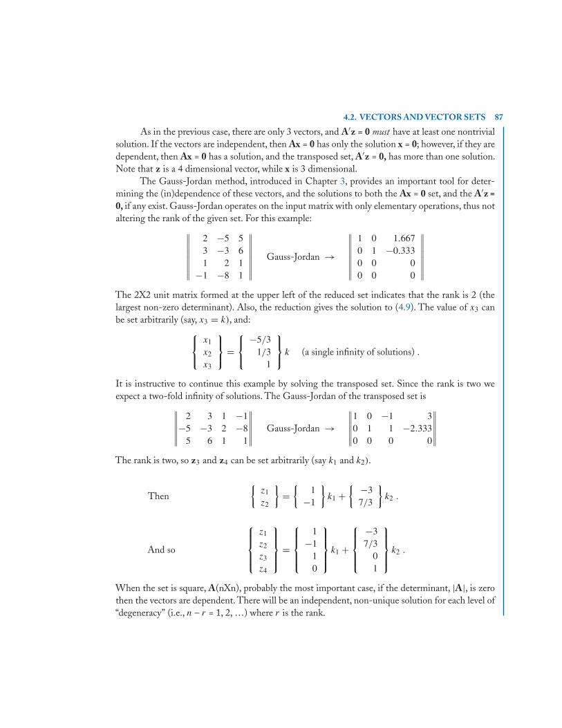
4.2. VECTORS AND VECTOR SETS 87
As in the previous case, there are only 3 vectors, and A′z = 0 must have at least one nontrivialsolution. If the vectors are independent, then Ax = 0 has only the solution x = 0; however, if they aredependent, then Ax = 0 has a solution, and the transposed set, A′z = 0, has more than one solution.Note that z is a 4 dimensional vector, while x is 3 dimensional.
The Gauss-Jordan method, introduced in Chapter 3, provides an important tool for deter-mining the (in)dependence of these vectors, and the solutions to both the Ax = 0 set, and the A′z =0, if any exist. Gauss-Jordan operates on the input matrix with only elementary operations, thus notaltering the rank of the given set. For this example:∥∥∥∥∥∥∥∥
2 −5 53 −3 61 2 1
−1 −8 1
∥∥∥∥∥∥∥∥Gauss-Jordan →
∥∥∥∥∥∥∥∥1 0 1.6670 1 −0.3330 0 00 0 0
∥∥∥∥∥∥∥∥The 2X2 unit matrix formed at the upper left of the reduced set indicates that the rank is 2 (thelargest non-zero determinant). Also, the reduction gives the solution to (4.9). The value of x3 canbe set arbitrarily (say, x3 = k), and:⎧⎨
⎩x1
x2
x3
⎫⎬⎭ =
⎧⎨⎩
−5/31/3
1
⎫⎬⎭ k (a single infinity of solutions) .
It is instructive to continue this example by solving the transposed set. Since the rank is two weexpect a two-fold infinity of solutions. The Gauss-Jordan of the transposed set is∥∥∥∥∥∥
2 3 1 −1−5 −3 2 −8
5 6 1 1
∥∥∥∥∥∥ Gauss-Jordan →∥∥∥∥∥∥
1 0 −1 30 1 1 −2.3330 0 0 0
∥∥∥∥∥∥The rank is two, so z3 and z4 can be set arbitrarily (say k1 and k2).
Then{
z1
z2
}={
1−1
}k1 +
{ −37/3
}k2 .
And so
⎧⎪⎪⎨⎪⎪⎩
z1
z2
z3
z4
⎫⎪⎪⎬⎪⎪⎭ =
⎧⎪⎪⎨⎪⎪⎩
1−1
10
⎫⎪⎪⎬⎪⎪⎭ k1 +
⎧⎪⎪⎨⎪⎪⎩
−37/3
01
⎫⎪⎪⎬⎪⎪⎭ k2 .
When the set is square, A(nXn), probably the most important case, if the determinant, |A|, is zerothen the vectors are dependent. There will be an independent, non-unique solution for each level of“degeneracy” (i.e., n – r = 1, 2, …) where r is the rank.
88 4. LINEAR SIMULTANEOUS EQUATION SETS
4.3 SIMULTANEOUS EQUATION SETSThis section considers equation sets, Ax = c in which the right-hand side, c, is non-zero.The equationset can be viewed as a vector transformation in which {c} is to be synthesized by a linear weightedsum of the left-hand column vectors (if possible). The problem is to find the weight factors (theelements of the x column).
4.3.1 SQUARE EQUATION SETSWriting Equation (4.1) as a vector equation, with m = n (“Square”):
A(nXn)x=y ⇒
⎧⎪⎪⎪⎨⎪⎪⎪⎩
a11
a21...
an1
⎫⎪⎪⎪⎬⎪⎪⎪⎭
x1 +
⎧⎪⎪⎪⎨⎪⎪⎪⎩
a12
a22...
an2
⎫⎪⎪⎪⎬⎪⎪⎪⎭
x2 + · · · +
⎧⎪⎪⎪⎨⎪⎪⎪⎩
a1n
a2n
...
ann
⎫⎪⎪⎪⎬⎪⎪⎪⎭
xn = y =
⎧⎪⎪⎪⎨⎪⎪⎪⎩
y1
y2...
yn
⎫⎪⎪⎪⎬⎪⎪⎪⎭
. (4.11)
The columns of A are the vectors to be added, using weighting factors, xj , resulting in an outputvector y. These equations are definitely “coupled” (into a single vector equation). But, if a vector,say, v1, could be found, that is simultaneously orthogonal to (i.e., perpendicular to) all the a vectorsin (4.11) save the first — that is:
v1 • aj = 0; for j=2, 3, · · · n .
Then, we could dot v1 through (4.11):
(v1 • a1)x1 + (v1 • a2)x2 + · · · + (v1 • an)xn = (v1 • y) . (4.12)
All the products (v1 • aj ) are zero, except the first (i.e., j = 1). Then: (v1 • a1)x1 = (v1 • y), and:
x1 = (v1 • y)
(v1 • a1). (4.13)
Next, if a vector v2 could be found that is orthogonal to all except a2 then the same procedure couldbe used to uncouple x2 from the rest. And, so on. Of course, it may not be easy to find successivevectors, vj , such that each is orthogonal to all but the j th a-vector. But, in 2 and three dimensionsit is easy. A “2-space” example is:
given Ax = y ⇒[ −2 1
0 2
]{x1
x2
}={ −2
0
}x1 +
{12
}x2 = y =
{1
−2
}. (4.14)
Choose v1 = {2, –1} and v2 = {0, 1}. Then:
[2 −1
] { −20
}x1 = [
2 −1] { 1
−2
}⇒ x1 = −1
and[
0 1] { 1
2
}x2 = [
0 1] { 1
−2
}⇒ x2 = −1 .
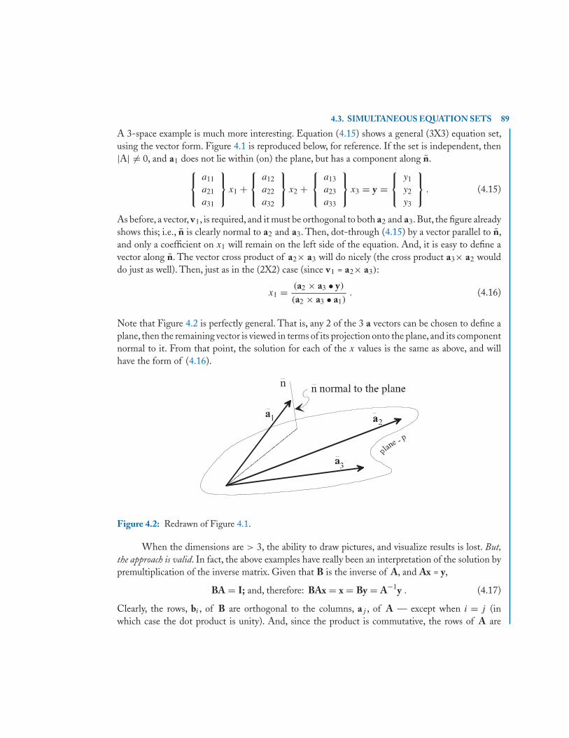
4.3. SIMULTANEOUS EQUATION SETS 89
A 3-space example is much more interesting. Equation (4.15) shows a general (3X3) equation set,using the vector form. Figure 4.1 is reproduced below, for reference. If the set is independent, then|A| �= 0, and a1 does not lie within (on) the plane, but has a component along n.⎧⎨
⎩a11
a21
a31
⎫⎬⎭ x1 +
⎧⎨⎩
a12
a22
a32
⎫⎬⎭ x2 +
⎧⎨⎩
a13
a23
a33
⎫⎬⎭ x3 = y =
⎧⎨⎩
y1
y2
y3
⎫⎬⎭ . (4.15)
As before, a vector, v1, is required, and it must be orthogonal to both a2 and a3. But, the figure alreadyshows this; i.e., n is clearly normal to a2 and a3. Then, dot-through (4.15) by a vector parallel to n,and only a coefficient on x1 will remain on the left side of the equation. And, it is easy to define avector along n. The vector cross product of a2× a3 will do nicely (the cross product a3× a2 woulddo just as well). Then, just as in the (2X2) case (since v1 = a2× a3):
x1 = (a2 × a3 • y)
(a2 × a3 • a1). (4.16)
Note that Figure 4.2 is perfectly general. That is, any 2 of the 3 a vectors can be chosen to define aplane, then the remaining vector is viewed in terms of its projection onto the plane, and its componentnormal to it. From that point, the solution for each of the x values is the same as above, and willhave the form of (4.16).
Figure 4.2: Redrawn of Figure 4.1.
When the dimensions are > 3, the ability to draw pictures, and visualize results is lost. But,the approach is valid. In fact, the above examples have really been an interpretation of the solution bypremultiplication of the inverse matrix. Given that B is the inverse of A, and Ax = y,
BA = I; and, therefore: BAx = x = By = A−1y . (4.17)
Clearly, the rows, bi , of B are orthogonal to the columns, aj , of A — except when i = j (inwhich case the dot product is unity). And, since the product is commutative, the rows of A are
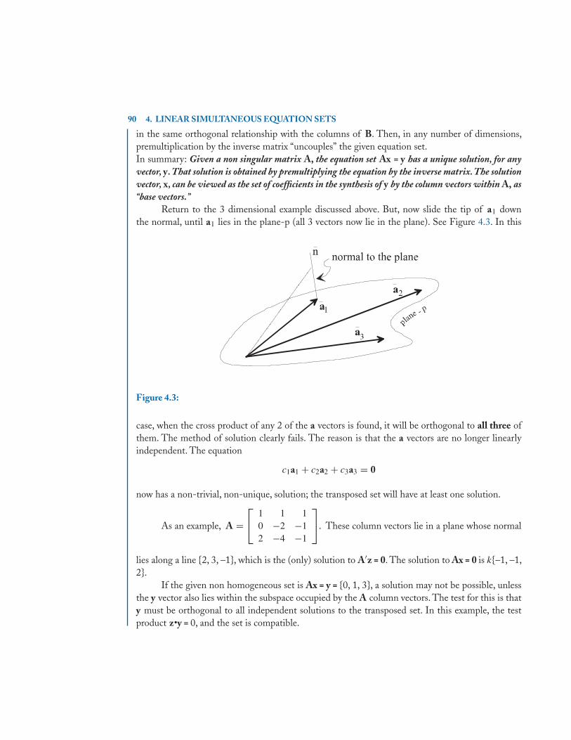
90 4. LINEAR SIMULTANEOUS EQUATION SETS
in the same orthogonal relationship with the columns of B. Then, in any number of dimensions,premultiplication by the inverse matrix “uncouples” the given equation set.In summary: Given a non singular matrix A, the equation set Ax = y has a unique solution, for anyvector, y. That solution is obtained by premultiplying the equation by the inverse matrix. The solutionvector, x, can be viewed as the set of coefficients in the synthesis of y by the column vectors within A, as“base vectors.”
Return to the 3 dimensional example discussed above. But, now slide the tip of a1 downthe normal, until a1 lies in the plane-p (all 3 vectors now lie in the plane). See Figure 4.3. In this
Figure 4.3:
case, when the cross product of any 2 of the a vectors is found, it will be orthogonal to all three ofthem. The method of solution clearly fails. The reason is that the a vectors are no longer linearlyindependent. The equation
c1a1 + c2a2 + c3a3 = 0
now has a non-trivial, non-unique, solution; the transposed set will have at least one solution.
As an example, A =⎡⎣ 1 1 1
0 −2 −12 −4 −1
⎤⎦. These column vectors lie in a plane whose normal
lies along a line {2, 3, –1}, which is the (only) solution to A′z = 0. The solution to Ax = 0 is k{–1, –1,2}.
If the given non homogeneous set is Ax = y = {0, 1, 3}, a solution may not be possible, unlessthe y vector also lies within the subspace occupied by the A column vectors. The test for this is thaty must be orthogonal to all independent solutions to the transposed set. In this example, the testproduct z•y = 0, and the set is compatible.
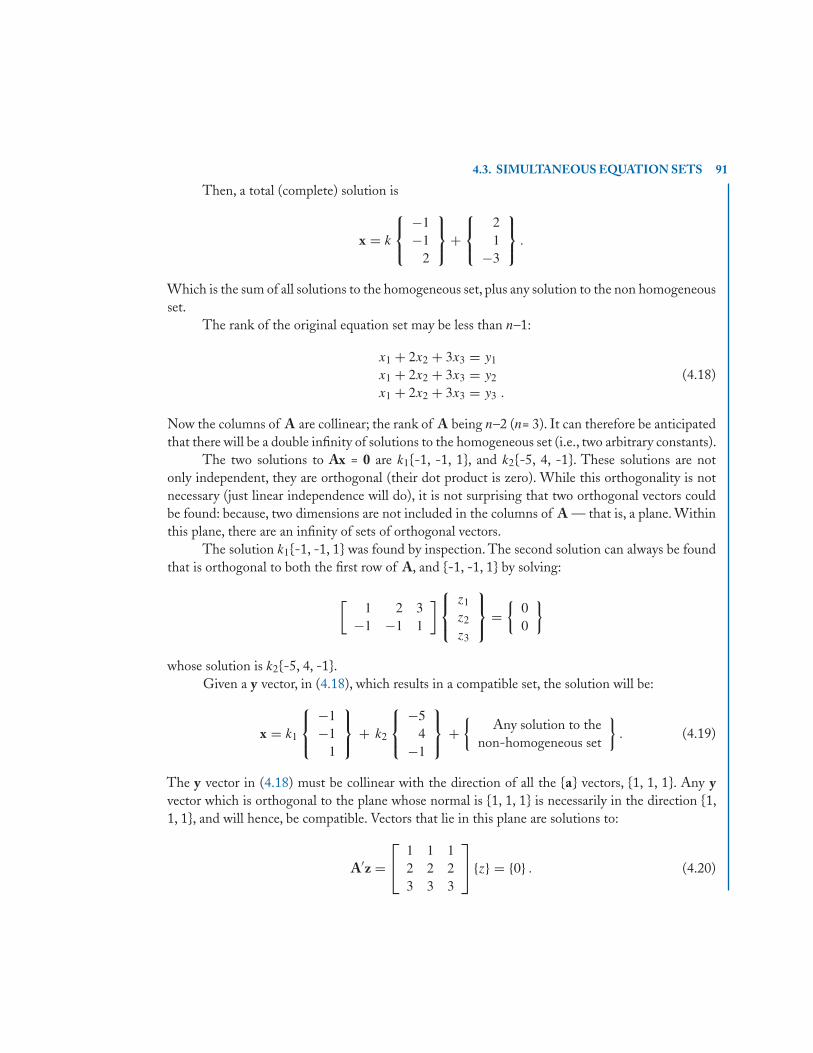
4.3. SIMULTANEOUS EQUATION SETS 91
Then, a total (complete) solution is
x = k
⎧⎨⎩
−1−1
2
⎫⎬⎭+
⎧⎨⎩
21
−3
⎫⎬⎭ .
Which is the sum of all solutions to the homogeneous set, plus any solution to the non homogeneousset.
The rank of the original equation set may be less than n–1:
x1 + 2x2 + 3x3 = y1
x1 + 2x2 + 3x3 = y2
x1 + 2x2 + 3x3 = y3 .
(4.18)
Now the columns of A are collinear; the rank of A being n–2 (n= 3). It can therefore be anticipatedthat there will be a double infinity of solutions to the homogeneous set (i.e., two arbitrary constants).
The two solutions to Ax = 0 are k1{-1, -1, 1}, and k2{-5, 4, -1}. These solutions are notonly independent, they are orthogonal (their dot product is zero). While this orthogonality is notnecessary (just linear independence will do), it is not surprising that two orthogonal vectors couldbe found: because, two dimensions are not included in the columns of A — that is, a plane. Withinthis plane, there are an infinity of sets of orthogonal vectors.
The solution k1{-1, -1, 1} was found by inspection. The second solution can always be foundthat is orthogonal to both the first row of A, and {-1, -1, 1} by solving:
[1 2 3
−1 −1 1
]⎧⎨⎩
z1
z2
z3
⎫⎬⎭ =
{00
}
whose solution is k2{-5, 4, -1}.Given a y vector, in (4.18), which results in a compatible set, the solution will be:
x = k1
⎧⎨⎩
−1−1
1
⎫⎬⎭ + k2
⎧⎨⎩
−54
−1
⎫⎬⎭ +
{Any solution to the
non-homogeneous set
}. (4.19)
The y vector in (4.18) must be collinear with the direction of all the {a} vectors, {1, 1, 1}. Any yvector which is orthogonal to the plane whose normal is {1, 1, 1} is necessarily in the direction {1,1, 1}, and will hence, be compatible. Vectors that lie in this plane are solutions to:
A′z =⎡⎣ 1 1 1
2 2 23 3 3
⎤⎦ {z} = {0} . (4.20)
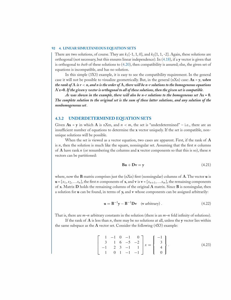
92 4. LINEAR SIMULTANEOUS EQUATION SETS
There are two solutions, of course. They are k1{-1, 1, 0}, and k2{1, 1, -2}. Again, these solutions areorthogonal (not necessary, but this ensures linear independence). In (4.18), if a y vector is given thatis orthogonal to both of these solutions to (4.20), then compatibility is assured; else, the given set ofequations is incompatible, and has no solution.
In this simple (3X3) example, it is easy to see the compatibility requirement. In the generalcase it will not be possible to visualize geometrically. But, in the general (nXn) case: Ax = y, whenthe rank of A is r < n, and n is the order of A, there will be n-r solutions to the homogeneous equationsA′z=0. If the given y vector is orthogonal to all of these solutions, then the given set is compatible.
As was shown in the example, there will also be n-r solutions to the homogeneous set Ax = 0.The complete solution to the original set is the sum of these latter solutions, and any solution of thenonhomogeneous set .
4.3.2 UNDERDETERMINED EQUATION SETSGiven Ax = y in which A is nXm, and n < m, the set is “underdetermined” – i.e., there are aninsufficient number of equations to determine the x vector uniquely. If the set is compatible, non-unique solutions will be possible.
When the set is viewed as a vector equation, two cases are apparent. First, if the rank of Ais n, then the solution is much like the square, nonsingular set. Assuming that the first n columnsof A have rank n (or renumbering the columns and x vector components so that this is so), these n
vectors can be partitioned:
Bu + Dv = y (4.21)
where, now the B matrix comprises just the (nXn) first (nonsingular) columns of A. The vector u isu = {x1, x2, …xn}, the first n components of x, and v is v = {xn+1, …xm}, the remaining componentsof x. Matrix D holds the remaining columns of the original A matrix. Since B is nonsingular, thena solution for u can be found, in terms of y, and v whose components can be assigned arbitrarily:
u = B−1y − B−1Dv (v arbitrary) . (4.22)
That is, there are m–n arbitrary constants in the solution (there is an m–n fold infinity of solutions).If the rank of A is less than n, there may be no solutions at all, unless the y vector lies within
the same subspace as the A vector set. Consider the following (4X5) example:
⎡⎢⎢⎣
1 −1 0 −1 03 1 6 −5 −2
−1 2 3 −1 11 0 1 −1 −1
⎤⎥⎥⎦ x =
⎧⎪⎪⎨⎪⎪⎩
−1340
⎫⎪⎪⎬⎪⎪⎭ . (4.23)
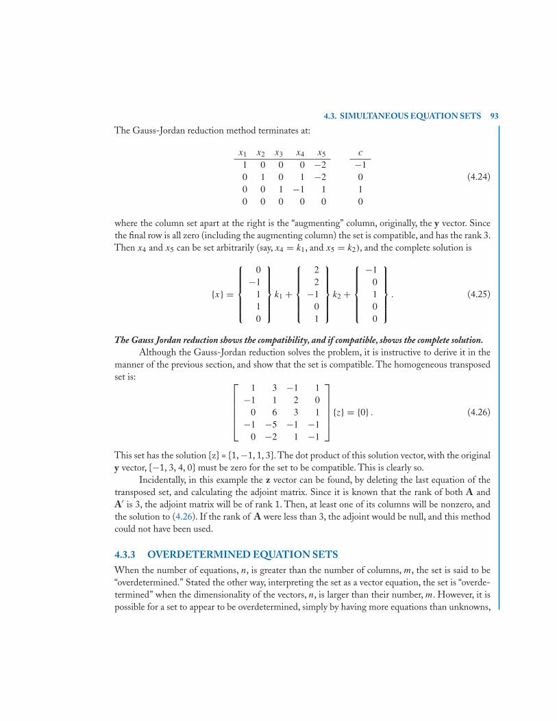
4.3. SIMULTANEOUS EQUATION SETS 93
The Gauss-Jordan reduction method terminates at:
x1 x2 x3 x4 x5
1 0 0 0 −20 1 0 1 −20 0 1 −1 10 0 0 0 0
c
−1010
(4.24)
where the column set apart at the right is the “augmenting” column, originally, the y vector. Sincethe final row is all zero (including the augmenting column) the set is compatible, and has the rank 3.Then x4 and x5 can be set arbitrarily (say, x4 = k1, and x5 = k2), and the complete solution is
{x} =
⎧⎪⎪⎪⎪⎨⎪⎪⎪⎪⎩
0−1
110
⎫⎪⎪⎪⎪⎬⎪⎪⎪⎪⎭
k1 +
⎧⎪⎪⎪⎪⎨⎪⎪⎪⎪⎩
22
−101
⎫⎪⎪⎪⎪⎬⎪⎪⎪⎪⎭
k2 +
⎧⎪⎪⎪⎪⎨⎪⎪⎪⎪⎩
−10100
⎫⎪⎪⎪⎪⎬⎪⎪⎪⎪⎭
. (4.25)
The Gauss Jordan reduction shows the compatibility, and if compatible, shows the complete solution.Although the Gauss-Jordan reduction solves the problem, it is instructive to derive it in the
manner of the previous section, and show that the set is compatible. The homogeneous transposedset is: ⎡
⎢⎢⎢⎢⎣1 3 −1 1
−1 1 2 00 6 3 1
−1 −5 −1 −10 −2 1 −1
⎤⎥⎥⎥⎥⎦ {z} = {0} . (4.26)
This set has the solution {z} = {1, −1, 1, 3}. The dot product of this solution vector, with the originaly vector, {−1, 3, 4, 0} must be zero for the set to be compatible. This is clearly so.
Incidentally, in this example the z vector can be found, by deleting the last equation of thetransposed set, and calculating the adjoint matrix. Since it is known that the rank of both A andA′ is 3, the adjoint matrix will be of rank 1. Then, at least one of its columns will be nonzero, andthe solution to (4.26). If the rank of A were less than 3, the adjoint would be null, and this methodcould not have been used.
4.3.3 OVERDETERMINED EQUATION SETSWhen the number of equations, n, is greater than the number of columns, m, the set is said to be“overdetermined.” Stated the other way, interpreting the set as a vector equation, the set is “overde-termined” when the dimensionality of the vectors, n, is larger than their number, m. However, it ispossible for a set to appear to be overdetermined, simply by having more equations than unknowns,
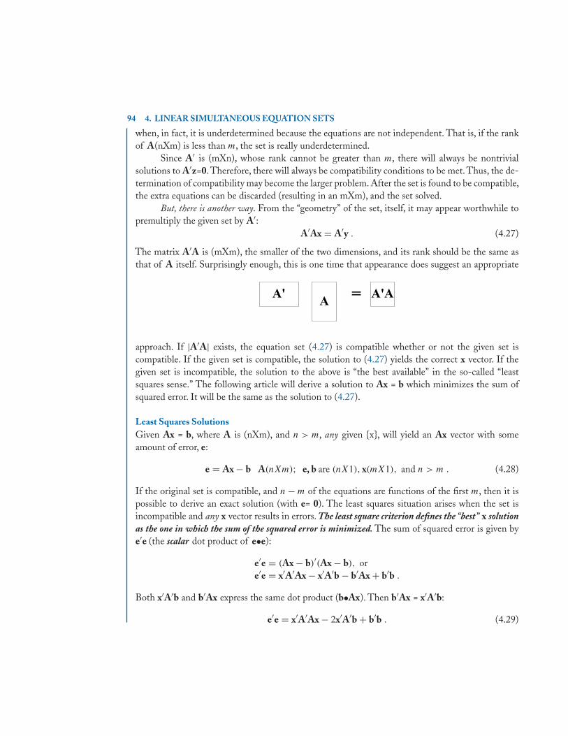
94 4. LINEAR SIMULTANEOUS EQUATION SETS
when, in fact, it is underdetermined because the equations are not independent. That is, if the rankof A(nXm) is less than m, the set is really underdetermined.
Since A′ is (mXn), whose rank cannot be greater than m, there will always be nontrivialsolutions to A′z=0. Therefore, there will always be compatibility conditions to be met. Thus, the de-termination of compatibility may become the larger problem. After the set is found to be compatible,the extra equations can be discarded (resulting in an mXm), and the set solved.
But, there is another way. From the “geometry” of the set, itself, it may appear worthwhile topremultiply the given set by A′:
A′Ax = A′y . (4.27)
The matrix A′A is (mXm), the smaller of the two dimensions, and its rank should be the same asthat of A itself. Surprisingly enough, this is one time that appearance does suggest an appropriate
approach. If |A′A| exists, the equation set (4.27) is compatible whether or not the given set iscompatible. If the given set is compatible, the solution to (4.27) yields the correct x vector. If thegiven set is incompatible, the solution to the above is “the best available” in the so-called “leastsquares sense.” The following article will derive a solution to Ax = b which minimizes the sum ofsquared error. It will be the same as the solution to (4.27).
Least Squares SolutionsGiven Ax = b, where A is (nXm), and n > m, any given {x}, will yield an Ax vector with someamount of error, e:
e = Ax − b A(nXm); e, b are (nX1), x(mX1), and n > m . (4.28)
If the original set is compatible, and n − m of the equations are functions of the first m, then it ispossible to derive an exact solution (with e= 0). The least squares situation arises when the set isincompatible and any x vector results in errors. The least square criterion defines the “best” x solutionas the one in which the sum of the squared error is minimized. The sum of squared error is given bye′e (the scalar dot product of e•e):
e′e = (Ax − b)′(Ax − b), ore′e = x′A′Ax − x′A′b − b′Ax + b′b .
Both x′A′b and b′Ax express the same dot product (b•Ax). Then b′Ax = x′A′b:
e′e = x′A′Ax − 2x′A′b + b′b . (4.29)
4.3. SIMULTANEOUS EQUATION SETS 95
The (scalar) term x′A′Ax is called a “quadratic” form, because in its expansion, the variables appearas a second degree product, xixj , in every term. Also required in the definition is that the (necessarilysquare) matrix be symmetric. Note that A′A is symmetric.The term x′A′b could be called a “bilinearform,” if one considers the b vector as a variable. In that case, xibj appear as products (hence “bi-linear”). It is not required that the matrix (A′, in this case), be symmetric; and, indeed, A′ is not (it’snot even square).The method is to take the partial derivatives of e′e with respect to each of the m variables, xi, in turn,and equate them simultaneously to zero. The resultant x vector minimizes e′e.⎧⎪⎪⎪⎪⎪⎪⎪⎪⎪⎨
⎪⎪⎪⎪⎪⎪⎪⎪⎪⎩
∂e′e∂x1
∂e′e∂x2
...
∂e′e∂xm
⎫⎪⎪⎪⎪⎪⎪⎪⎪⎪⎬⎪⎪⎪⎪⎪⎪⎪⎪⎪⎭
= {0} . (4.30)
The solution to the equation set that results from (4.30) is the x vector which minimizes e′e.Appendix A discusses the partial differentiation of bilinear and quadratic forms. It begins by definingthe vector differential operator, ∇.
∇ =
⎧⎪⎪⎪⎪⎪⎪⎪⎪⎪⎨⎪⎪⎪⎪⎪⎪⎪⎪⎪⎩
∂
∂ x1
∂
∂ x2...
∂
∂ xm
⎫⎪⎪⎪⎪⎪⎪⎪⎪⎪⎬⎪⎪⎪⎪⎪⎪⎪⎪⎪⎭
. (4.31)
Using this definition (4.30) becomes ∇e′e = 0 and from (4.29)
∇ e′e = ∇(x′A′Ax) − ∇ (2x′A′b) + ∇ (b′b) = 0 . (4.32)
The b vector is not a function of x, so the last term is 0. Appendix A finds ∇(x′A′Ax) = 2A′Ax, and∇(2x′A′b) = 2A′b. Then:
∇e′e = 2A′Ax − 2A′b = {0} (4.33)A′Ax = A′b (see Equation (4.27)) . (4.34)
This remarkable result indicates that the minimum squared error will be obtained when the x vectoris defined by solution to the square (mXm) set of (4.34). The original A is nXm, so A′A is mXm).By hypothesis A has the rank m, so A′A is nonsingular giving
x = (A′A)−1A′b . (4.35)
What’s more, if the original set is compatible, (4.35) yields the unique solution!

96 4. LINEAR SIMULTANEOUS EQUATION SETS
4.4 LINEAR REGRESSIONThe engineering sciences are based upon physical entities and the relationships between them.However, the relationships are most often expressed in exact equation form, implying a knowledgeof the exact values of the variables they contain. Usually, this is not the case. Many physical variablesare the result of empirical measurement. For example, in dynamics, a velocity or acceleration is knownas a result of observations. It may be known accurately, but not exactly.
Over a limited range the relationship between variables, though not known, may be assumedto be linear. Then, “linear regression” is used to determine a “best” straight line relationship. Mostoften, a least squares fit to the data is chosen to define the “best fit.” There are some good statisticalreasons for this choice; and (perhaps the most compelling reason) the least squares analysis is easyto perform.
It has already been decided that the relationship between a dependent variable, y, known onlyby a set of observed data points, yi , and an independent variable, x, is a linear curve, part of whichis shown in Figure 4.4.
y = c1x + c2 . (4.36)
If exact (x, y) data could be obtained, it would only take two pairs to determine c1 and c2. But,
Figure 4.4:
the relationship between x and y is a complicated one and the data contains observation errors.The problem is, then, to determine a “best fit” curve so that other y-data can be predicted fromgiven x-data. “Best” is determined to be a least squares fit to the data. In general, quite a few(x, y) measurements are taken over the range of interest, in an attempt to “average-out” as muchobservation error as possible. Thus, if an equation yi = c1xi + c2 is written for every one of theobservations, a very overdetermined equation set results.
The xi data need not be equi-spaced (as implied by Fig. 4.4), and some (but not all) of the yi
points may be redundant measurements at the same value of xi . The objective is, of course, to allowthe error to “average out,” yielding a regression line that is accurate to within the requirements ofthe physical problem.
Then, given the set of N observed (x, y) data points, write:
y = Xc = [X]{c} (4.37)
4.4. LINEAR REGRESSION 97
where y = {yi}, the y observed data, and X containing the x-data:
X =
⎡⎢⎢⎣
x1 1x2 1· · · · · ·xN 1
⎤⎥⎥⎦ c =
{c1
c2
}y =
⎧⎪⎪⎪⎨⎪⎪⎪⎩
y1
y2...
yN
⎫⎪⎪⎪⎬⎪⎪⎪⎭
.
Equation (4.37) is an overdetermined (NX2) set of linear equations in the unknown variables c1 andc2. The previous article, and Equation (4.35), provide the solution:
c = (X′X)−1[X′]y . (4.38)
In (4.38), the X′X matrix is 2X2, clearly symmetric and nonsingular, unless the data is all at the samexi . The columns {c} and [X′]y are 2X1 (X′ is 2XN, times y(NX1)).
X′X =[ ∑
x2i
∑xi∑
xi N
]X′y =
[ ∑xiyi∑
yi
]. (4.39)
In these equations, the summations are to be taken over the index, i, from 1 to N. To avoid messymatrix terms, the inverse of X′X will be expressed in terms of its adjoint and its determinant in thefollowing:
[X′X
]adj =[
N −∑xi
−∑xi
∑x2i
] ∣∣X′X∣∣ = N
∑x2i −
(∑xi
)2. (4.40)
Carrying out the product terms indicated in (4.38), the solutions for c1 and c2 are:
c1 = N∑
xiyi −∑xi
∑yi
N∑
x2i − (
∑xi)2
(4.41)
c2 =∑
x2i
∑yi −∑
xi
∑xiyi
N∑
x2i − (
∑xi)2
. (4.42)
Some additional algebraic work can be done on these two equations, which will result in an ap-pearance that is much more appealing. First, define the average values of yi and xi as x and y,where:
x =∑
xi
Nand y =
∑yi
N.
To reduce c2, subtract y from both sides of (4.42):
c2 − y =∑
x2i
∑yi −∑
xi
∑xiyi
N∑
x2i − (
∑xi)2
−∑
yi
N. (4.43)
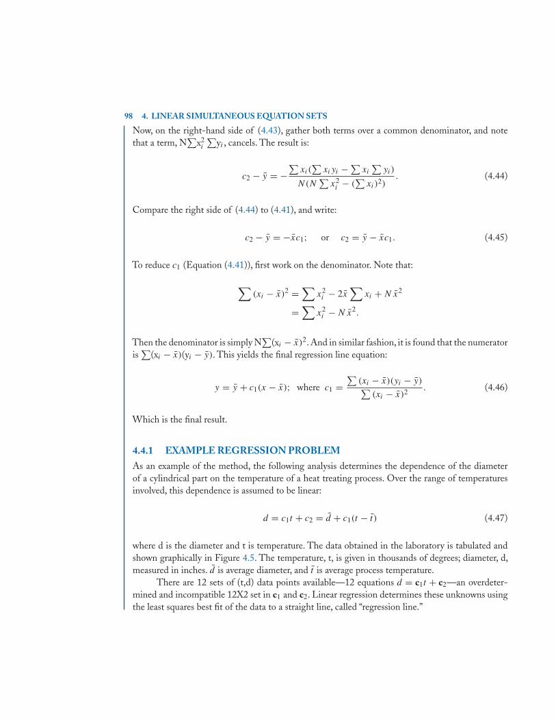
98 4. LINEAR SIMULTANEOUS EQUATION SETS
Now, on the right-hand side of (4.43), gather both terms over a common denominator, and notethat a term, N
∑x2i
∑yi , cancels. The result is:
c2 − y = −∑
xi(∑
xiyi −∑xi
∑yi)
N(N∑
x2i − (
∑xi)2)
. (4.44)
Compare the right side of (4.44) to (4.41), and write:
c2 − y = −xc1; or c2 = y − xc1. (4.45)
To reduce c1 (Equation (4.41)), first work on the denominator. Note that:
∑(xi − x)2 =
∑x2i − 2x
∑xi + N x2
=∑
x2i − N x2.
Then the denominator is simply N∑
(xi − x)2. And in similar fashion, it is found that the numeratoris∑
(xi − x)(yi − y). This yields the final regression line equation:
y = y + c1(x − x); where c1 =∑
(xi − x)(yi − y)∑(xi − x)2
. (4.46)
Which is the final result.
4.4.1 EXAMPLE REGRESSION PROBLEMAs an example of the method, the following analysis determines the dependence of the diameterof a cylindrical part on the temperature of a heat treating process. Over the range of temperaturesinvolved, this dependence is assumed to be linear:
d = c1t + c2 = d + c1(t − t ) (4.47)
where d is the diameter and t is temperature. The data obtained in the laboratory is tabulated andshown graphically in Figure 4.5. The temperature, t, is given in thousands of degrees; diameter, d,measured in inches. d is average diameter, and t is average process temperature.
There are 12 sets of (t,d) data points available—12 equations d = c1t + c2—an overdeter-mined and incompatible 12X2 set in c1 and c2. Linear regression determines these unknowns usingthe least squares best fit of the data to a straight line, called “regression line.”
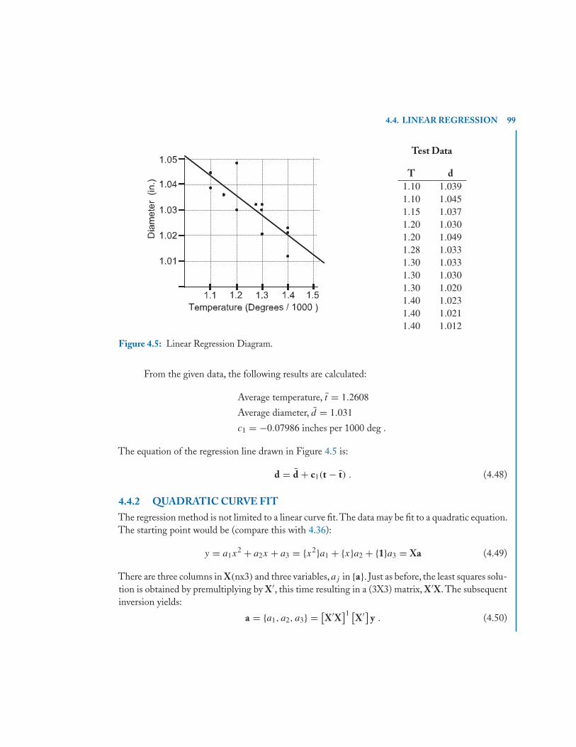
4.4. LINEAR REGRESSION 99
Figure 4.5: Linear Regression Diagram.
Test Data
T d1.10 1.0391.10 1.0451.15 1.0371.20 1.0301.20 1.0491.28 1.0331.30 1.0331.30 1.0301.30 1.0201.40 1.0231.40 1.0211.40 1.012
From the given data, the following results are calculated:
Average temperature, t = 1.2608
Average diameter, d = 1.031
c1 = −0.07986 inches per 1000 deg .
The equation of the regression line drawn in Figure 4.5 is:
d = d + c1(t − t) . (4.48)
4.4.2 QUADRATIC CURVE FITThe regression method is not limited to a linear curve fit.The data may be fit to a quadratic equation.The starting point would be (compare this with 4.36):
y = a1x2 + a2x + a3 = {x2}a1 + {x}a2 + {1}a3 = Xa (4.49)
There are three columns in X(nx3) and three variables,aj in {a}. Just as before, the least squares solu-tion is obtained by premultiplying by X′, this time resulting in a (3X3) matrix, X′X. The subsequentinversion yields:
a = {a1, a2, a3} = [X′X
]1 [X′] y . (4.50)
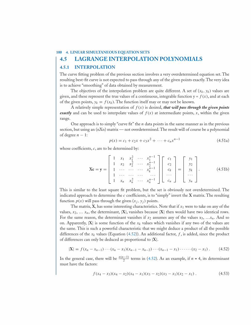
100 4. LINEAR SIMULTANEOUS EQUATION SETS
4.5 LAGRANGE INTERPOLATION POLYNOMIALS4.5.1 INTERPOLATIONThe curve fitting problem of the previous section involves a very overdetermined equation set. Theresulting best-fit curve is not expected to pass through any of the given points exactly. The very ideais to achieve “smoothing” of data obtained by measurement.
The objectives of the interpolation problem are quite different. A set of (xk, yk) values aregiven, and these represent the true values of a continuous, integrable function y = f (x), and at eachof the given points, yk = f (xk). The function itself may or may not be known.
A relatively simple representation of f (x) is desired, that will pass through the given pointsexactly and can be used to interpolate values of f (x) at intermediate points, x, within the givenrange.
One approach is to simply “curve fit” the n data points in the same manner as in the previoussection, but using an (nXn) matrix — not overdetermined. The result will of course be a polynomialof degree n − 1:
p(x) = c1 + c2x + c3x2 + · · · + cnx
n−1 (4.51a)
whose coefficients, c, are to be determined by:
Xc = y =
⎡⎢⎢⎢⎢⎢⎣
1 x1 x21 · · · xn−1
11 x2 x2
2 · · · xn−12
1 · · · · · · · · · xn−1k
1 · · · · · · · · · · · ·1 xn x2
n · · · xn−1n
⎤⎥⎥⎥⎥⎥⎦
⎡⎢⎢⎢⎢⎣
c1
c2
ck
· · ·cn
⎤⎥⎥⎥⎥⎦ =
⎡⎢⎢⎢⎢⎣
y1
y2
yk
· · ·yn
⎤⎥⎥⎥⎥⎦ . (4.51b)
This is similar to the least square fit problem, but the set is obviously not overdetermined. Theindicated approach to determine the c coefficients, is to “simply” invert the X matrix. The resultingfunction p(x) will pass through the given (xj , yj ) points.
The matrix, X, has some interesting characteristics. Note that if x1 were to take on any of thevalues, x2, … xn, the determinant, |X|, vanishes because |X| then would have two identical rows.For the same reason, the determinant vanishes if x2 assumes any of the values x3, …xn. And soon. Apparently, |X| is some function of the xk values which vanishes if any two of the values arethe same. This is such a powerful characteristic that we might deduce a product of all the possibledifferences of the xk values (Equation (4.52)). An additional factor, f , is added, since the productof differences can only be deduced as proportional to |X|.
|X| = f (xn − xn−1) · · · (xn − x1)(xn−1 − xn−2) · · · (xn−1 − x1) · · · · · · (x2 − x1) . (4.52)
In the general case, there will be n(n−1)2 terms in (4.52). As an example, if n = 4, its determinant
must have the factors:
f (x4 − x3)(x4 − x2)(x4 − x1)(x3 − x2)(x3 − x1)(x2 − x1) . (4.53)
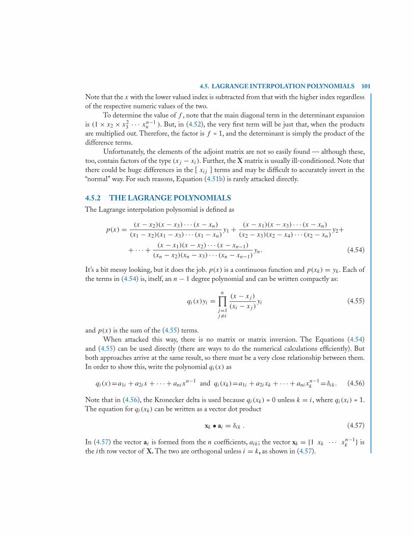
4.5. LAGRANGE INTERPOLATION POLYNOMIALS 101
Note that the x with the lower valued index is subtracted from that with the higher index regardlessof the respective numeric values of the two.
To determine the value of f , note that the main diagonal term in the determinant expansionis (1 × x2 × x2
3 · · · xn−1n ). But, in (4.52), the very first term will be just that, when the products
are multiplied out. Therefore, the factor is f = 1, and the determinant is simply the product of thedifference terms.
Unfortunately, the elements of the adjoint matrix are not so easily found — although these,too, contain factors of the type (xj − xi). Further, the X matrix is usually ill-conditioned. Note thatthere could be huge differences in the [ xij ] terms and may be difficult to accurately invert in the“normal” way. For such reasons, Equation (4.51b) is rarely attacked directly.
4.5.2 THE LAGRANGE POLYNOMIALSThe Lagrange interpolation polynomial is defined as
p(x) = (x − x2)(x − x3) · · · (x − xn)
(x1 − x2)(x1 − x3) · · · (x1 − xn)y1 + (x − x1)(x − x3) · · · (x − xn)
(x2 − x3)(x2 − x4) · · · (x2 − xn)y2+
+ · · · + (x − x1)(x − x2) · · · (x − xn−1)
(xn − x2)(xn − x3) · · · (xn − xn−1)yn. (4.54)
It’s a bit messy looking, but it does the job. p(x) is a continuous function and p(xk) = yk . Each ofthe terms in (4.54) is, itself, an n − 1 degree polynomial and can be written compactly as:
qi(x)yi =n∏
j=1j �=i
(x − xj )
(xi − xj )yi (4.55)
and p(x) is the sum of the (4.55) terms.When attacked this way, there is no matrix or matrix inversion. The Equations (4.54)
and (4.55) can be used directly (there are ways to do the numerical calculations efficiently). Butboth approaches arrive at the same result, so there must be a very close relationship between them.In order to show this, write the polynomial qi(x) as
qi(x)=a1i + a2ix + · · · + anixn−1 and qi(xk)=a1i + a2ixk + · · · + anix
n−1k =δik. (4.56)
Note that in (4.56), the Kronecker delta is used because qi(xk) = 0 unless k = i, where qi(xi) = 1.The equation for qi(xk) can be written as a vector dot product
xk • ai = δik . (4.57)
In (4.57) the vector ai is formed from the n coefficients, aik ; the vector xk = {1 xk · · · xn−1k } is
the ith row vector of X. The two are orthogonal unless i = k, as shown in (4.57).
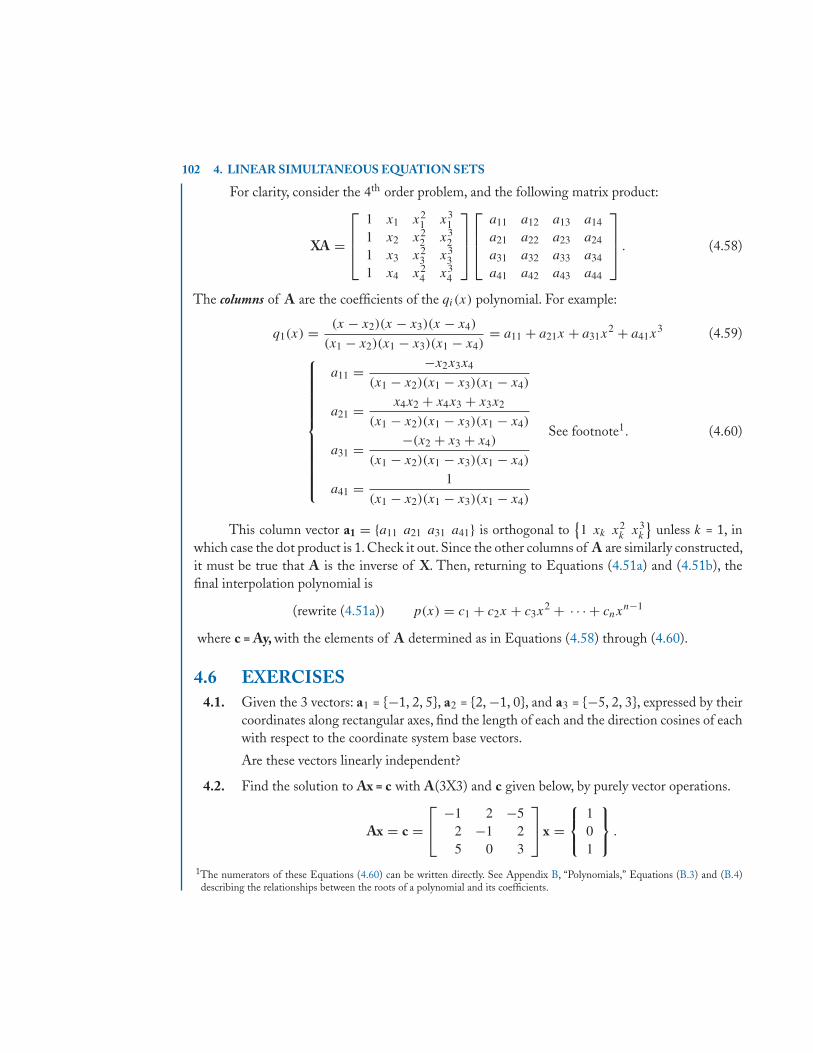
102 4. LINEAR SIMULTANEOUS EQUATION SETS
For clarity, consider the 4th order problem, and the following matrix product:
XA =
⎡⎢⎢⎣
1 x1 x21 x3
11 x2 x2
2 x32
1 x3 x23 x3
31 x4 x2
4 x34
⎤⎥⎥⎦⎡⎢⎢⎣
a11 a12 a13 a14
a21 a22 a23 a24
a31 a32 a33 a34
a41 a42 a43 a44
⎤⎥⎥⎦ . (4.58)
The columns of A are the coefficients of the qi(x) polynomial. For example:
q1(x) = (x − x2)(x − x3)(x − x4)
(x1 − x2)(x1 − x3)(x1 − x4)= a11 + a21x + a31x
2 + a41x3 (4.59)
⎧⎪⎪⎪⎪⎪⎪⎪⎪⎪⎪⎪⎨⎪⎪⎪⎪⎪⎪⎪⎪⎪⎪⎪⎩
a11 = −x2x3x4
(x1 − x2)(x1 − x3)(x1 − x4)
a21 = x4x2 + x4x3 + x3x2
(x1 − x2)(x1 − x3)(x1 − x4)
a31 = −(x2 + x3 + x4)
(x1 − x2)(x1 − x3)(x1 − x4)
a41 = 1
(x1 − x2)(x1 − x3)(x1 − x4)
See footnote1. (4.60)
This column vector a1 = {a11 a21 a31 a41} is orthogonal to{1 xk x2
k x3k
}unless k = 1, in
which case the dot product is 1. Check it out. Since the other columns of A are similarly constructed,it must be true that A is the inverse of X. Then, returning to Equations (4.51a) and (4.51b), thefinal interpolation polynomial is
(rewrite (4.51a)) p(x) = c1 + c2x + c3x2 + · · · + cnx
n−1
where c = Ay, with the elements of A determined as in Equations (4.58) through (4.60).
4.6 EXERCISES4.1. Given the 3 vectors: a1 = {−1, 2, 5}, a2 = {2, −1, 0}, and a3 = {−5, 2, 3}, expressed by their
coordinates along rectangular axes, find the length of each and the direction cosines of eachwith respect to the coordinate system base vectors.
Are these vectors linearly independent?
4.2. Find the solution to Ax = c with A(3X3) and c given below, by purely vector operations.
Ax = c =⎡⎣ −1 2 −5
2 −1 25 0 3
⎤⎦ x =
⎧⎨⎩
101
⎫⎬⎭ .
1The numerators of these Equations (4.60) can be written directly. See Appendix B, “Polynomials,” Equations (B.3) and (B.4)describing the relationships between the roots of a polynomial and its coefficients.
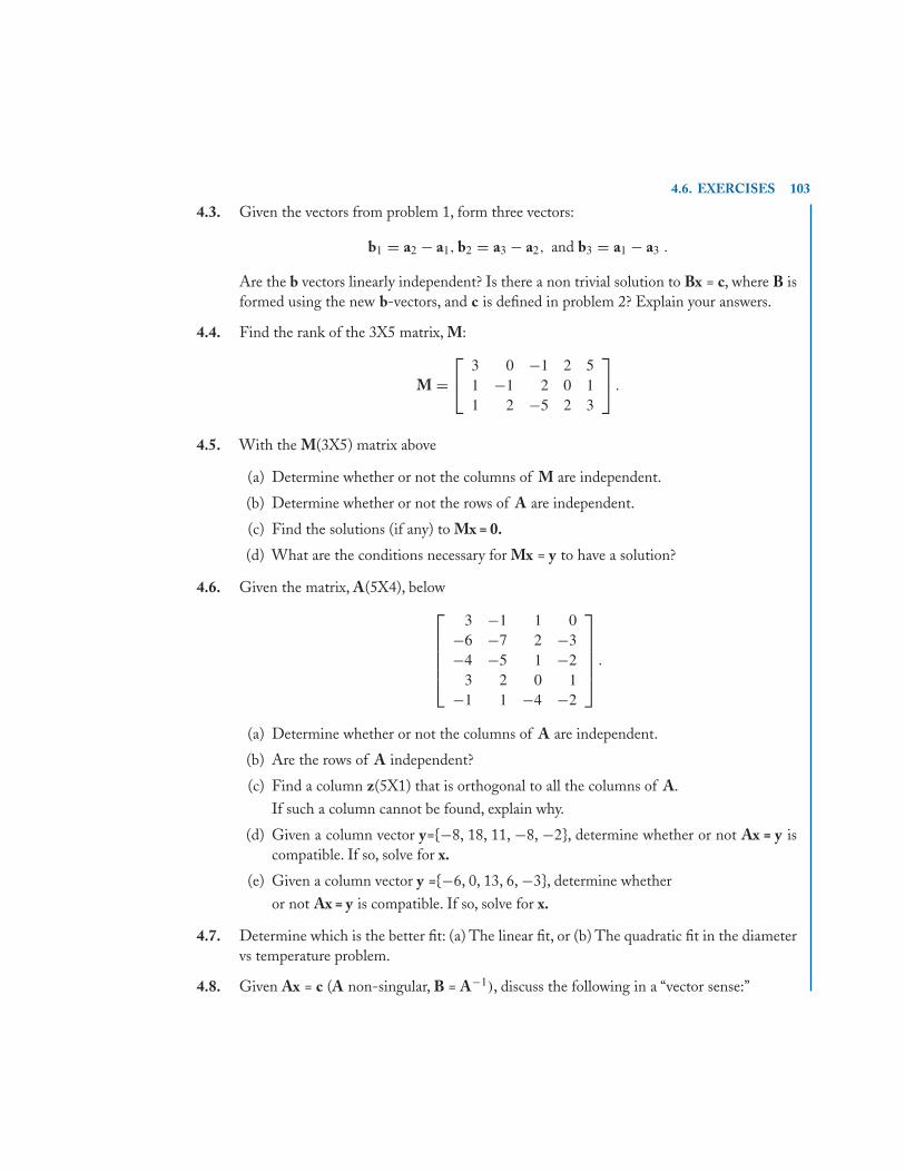
4.6. EXERCISES 103
4.3. Given the vectors from problem 1, form three vectors:
b1 = a2 − a1, b2 = a3 − a2, and b3 = a1 − a3 .
Are the b vectors linearly independent? Is there a non trivial solution to Bx = c, where B isformed using the new b-vectors, and c is defined in problem 2? Explain your answers.
4.4. Find the rank of the 3X5 matrix, M:
M =⎡⎣ 3 0 −1 2 5
1 −1 2 0 11 2 −5 2 3
⎤⎦ .
4.5. With the M(3X5) matrix above
(a) Determine whether or not the columns of M are independent.
(b) Determine whether or not the rows of A are independent.
(c) Find the solutions (if any) to Mx = 0.
(d) What are the conditions necessary for Mx = y to have a solution?
4.6. Given the matrix, A(5X4), below⎡⎢⎢⎢⎢⎣
3 −1 1 0−6 −7 2 −3−4 −5 1 −2
3 2 0 1−1 1 −4 −2
⎤⎥⎥⎥⎥⎦ .
(a) Determine whether or not the columns of A are independent.
(b) Are the rows of A independent?
(c) Find a column z(5X1) that is orthogonal to all the columns of A.If such a column cannot be found, explain why.
(d) Given a column vector y={−8, 18, 11, −8, −2}, determine whether or not Ax = y iscompatible. If so, solve for x.
(e) Given a column vector y ={−6, 0, 13, 6, −3}, determine whetheror not Ax = y is compatible. If so, solve for x.
4.7. Determine which is the better fit: (a) The linear fit, or (b) The quadratic fit in the diametervs temperature problem.
4.8. Given Ax = c (A non-singular, B = A−1), discuss the following in a “vector sense:”
104 4. LINEAR SIMULTANEOUS EQUATION SETS
(a) A columns i and j are interchanged, how is B affected? How is the solution, x, affected?
(b) A rows i and j are interchanged, how is B affected? How is the solution, x, affected?
(c) If rows i and j of the vector, c, are interchanged, how are B and x affected?
4.9. Determine whether or not there are values of the λ parameter for which a solution exists inthe equation set below. ⎡
⎣ λ −1 3−4 2 0
8 −λ 2λ
⎤⎦⎧⎨⎩
x1
x2
x3
⎫⎬⎭ =
⎧⎨⎩
000
⎫⎬⎭ .
(a) How many such values exist?
(b) For each one, find the general solution to the set.
4.10. Find the least squares best solution for c1 and c2 in the equation set below.
1.00c1 + c2 = 1.831.50c1 + c2 = 1.981.80c1 + c2 = 2.092.00c1 + c2 = 2.173.10c1 + c2 = 2.523.20c1 + c2 = 2.563.30c1 + c2 = 2.59 .
4.11. Using Equations (4.60) show that q1 • xj = δ1j where q1 is the vector formed from the
coefficients of the q1(x) polynomial and xj ={
1 xj x2j x3
j
}, the j th row of X.
4.12. Show that
|X| =∣∣∣∣∣∣
1 x21 x3
11 x2
3 x33
1 x24 x3
4
∣∣∣∣∣∣ = (x1x3 + x1x4 + x3x4)(x4 − x1)(x4 − x3)(x3 − x1).
Hint: Note the subscript numbering in |X|. Start with the X(4X4), and delete row andcolumn 2.
4.13. In the polynomial6∏
j=1(x − xj ) = x6 + c1x
5 + · · · + cn find c2 and c3. Describe the for-
mation of each of the coefficients.
105
C H A P T E R 5
Orthogonal Transforms
5.1 INTRODUCTIONThis chapter will explore other uses and characteristics of the transform equation Ax = y. In this newcase, however, the transform matrix will be an orthogonal one (see definition in Chapter 1); and so,it will not be denoted by the letter “A,” but, by some (hopefully more descriptive) letter — usually“T,” “P,” or “Q.”
This chapter will be largely “conceptual,” with emphasis on three dimensional thinking.We willbe concerned with physical displacements and motions in the real world; three linear displacementcoordinates, plus angular displacement, and motion, about the three coordinates. There will not bemuch extension of concept into n-space, although orthogonal transforms are certainly not limitedto 3-space. The next chapter will include some very interesting examples in n-space.
These are relatively simple concepts. But, they are of great value to the engineer, who is oftenrequired to conceptualize in three dimensions. The transform matrix will be seen to provide aninvaluable framework for his thinking, and approach to problem solving.
5.2 ORTHOGONAL MATRICES AND TRANSFORMSThe definition of an orthogonal matrix is one whose transpose is equal to its inverse. Then, giventhe orthogonal matrix, T:
T′ = T−1
TT′ = T′T = I .(5.1)
The dot product of any two columns (rows) of an orthogonal matrix is zero. The dot product of thecolumn (row) by itself is 1. Then, the orthogonal matrix is also “orthonormal.”
The usual function of such a matrix is to describe rotation in a 2 or 3-dimensional system.The transform equation x = Ty relates the coordinates of a vector as measured in two rectangularcoordinate systems. In two dimensions, consider two coordinate sets, x and y, that are collinear(superimposed). In this case, any vector, say r, has identical components when represented in eitherthe x-set, or the y-set. The transform relating coordinates in the two sets is y = Ix, where x and y
are 2X1 vectors representing coordinates in the x and y sets, and the transform matrix is the 2X2unit matrix (note that the unit matrix, I, is orthogonal). However, this case is trivial.
Next, the y-set is rotated in the + direction (counterclockwise) by an amount θ . Now, thecoordinates of r are different in the y-set, and there is a nontrivial, orthogonal, “transformation”between the two sets. We will define this transform.
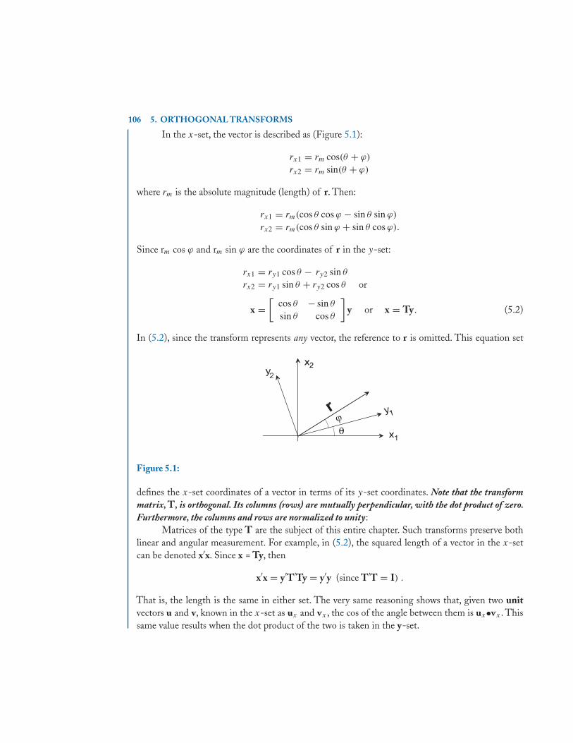
106 5. ORTHOGONAL TRANSFORMS
In the x-set, the vector is described as (Figure 5.1):
rx1 = rm cos(θ + ϕ)
rx2 = rm sin(θ + ϕ)
where rm is the absolute magnitude (length) of r. Then:
rx1 = rm(cos θ cos ϕ − sin θ sin ϕ)
rx2 = rm(cos θ sin ϕ + sin θ cos ϕ).
Since rm cos ϕ and rm sin ϕ are the coordinates of r in the y-set:
rx1 = ry1 cos θ − ry2 sin θ
rx2 = ry1 sin θ + ry2 cos θ or
x =[
cos θ − sin θ
sin θ cos θ
]y or x = Ty. (5.2)
In (5.2), since the transform represents any vector, the reference to r is omitted. This equation set
Figure 5.1:
defines the x-set coordinates of a vector in terms of its y-set coordinates. Note that the transformmatrix, T, is orthogonal. Its columns (rows) are mutually perpendicular, with the dot product of zero.Furthermore, the columns and rows are normalized to unity:
Matrices of the type T are the subject of this entire chapter. Such transforms preserve bothlinear and angular measurement. For example, in (5.2), the squared length of a vector in the x-setcan be denoted x′x. Since x = Ty, then
x′x = y′T′Ty = y′y (since T′T = I) .
That is, the length is the same in either set. The very same reasoning shows that, given two unitvectors u and v, known in the x-set as ux and vx , the cos of the angle between them is ux•vx . Thissame value results when the dot product of the two is taken in the y-set.
5.2. ORTHOGONAL MATRICES AND TRANSFORMS 107
In order to define the inverse transform of (5.2), we need only transpose the T matrix:
y =[
cos θ sin θ
− sin θ cos θ
]x or y = T ′x . (5.3)
Note that which matrix is called T, and which T′, is largely a matter of choice.So, of what use is this transform matrix? To see the answer, just consider the r vector in
motion. Conceptually, we attach this vector to the y-set . Its rotations are those of its coordinate set.And, we can simply describe any rectilinear motion in this set. Then, to see the total motion, we justtransform the vector back into the “inertial” (fixed) x-set.
The 3-dimensional case is a trivial extension of (5.2) and (5.3). From the Figure 5.1, above,just include the +x3 and +y3 axes coming directly upward – out of the plane of the page. Especiallynote that the rotation θ occurs around these axes; they therefore remain collinear (and the coordinateof any vector in this direction is measured the same in both x and y-sets). Then:
y =⎡⎣−
cos θ sin θ 0sin θ cos θ 0
0 0 1
⎤⎦ x . (5.4)
Equation (5.4) is the transform matrix between the inertial x-set, and a y-set, which has been rotatedby a + angle θ about the x3 axis. The inverse transform is simply the transpose of the matrix in (5.4).
5.2.1 RIGHTHANDED COORDINATES, AND POSITIVE ANGLEOne must be careful to describe a 3-dimensional coordinate set by the so called “right hand rule,”and to define positive angle in the same way. In Figure 5.1, the positive x1-axis is directed toward theright, the positive x2 axis upward (from the bottom of the page toward the top). Then, the positivex3 axis necessarily must come out of the page, toward you (the negative x3 axis is, then, directedaway from you, into the pages of the book). All of the coordinate sets constructed in this chapter willfollow this rule.
Another way to see this is: Curl the fingers of your right hand from the +1-axis to the +2-axis.Then, your thumb will point in the direction of the positive 3-axis. Now, do the same with the 2-axis,toward the 3-axis. The thumb will point to the positive 1-axis. Finally, assure yourself by curling theright fingers from the +3-axis toward the +1-axis. The thumb will now point toward positive 2-axis.See the next section, where the vector (cross) product is discussed.
Positive angle will be measured in the same sense: Rotation about any positive axis will itselfbe plus in the direction of the curled fingers of the right hand – counterclockwise, when the positiveaxis is in the same direction as the thumb.
These rules are very important. An incorrect sign can easily occur, and be very difficult to traceto a coordinate set improperly constructed.
Now, consider any orthogonal transform in which we regard the x-set as “stationary,” withthe y-set having undergone some series of rotations. In 3 dimensions, define unit vectors in both
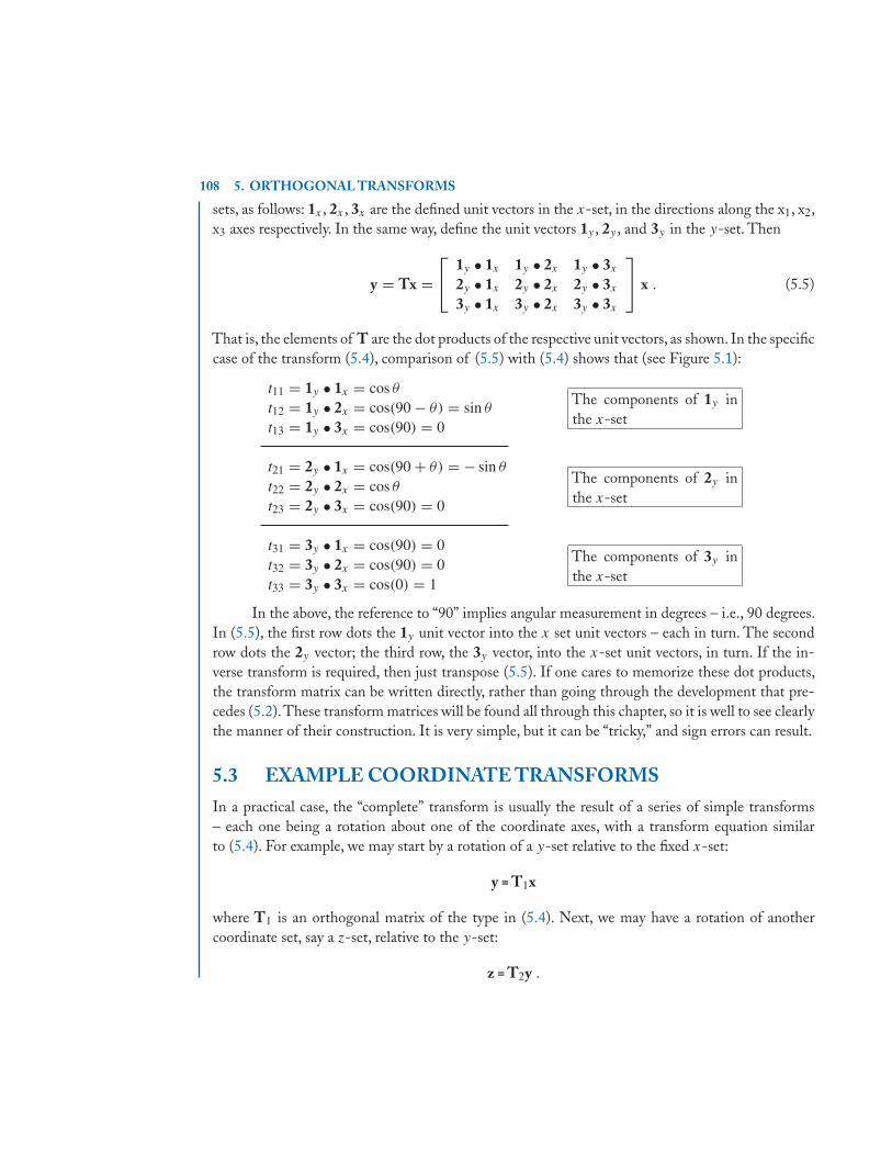
108 5. ORTHOGONAL TRANSFORMS
sets, as follows: 1x , 2x , 3x are the defined unit vectors in the x-set, in the directions along the x1, x2,x3 axes respectively. In the same way, define the unit vectors 1y , 2y , and 3y in the y-set. Then
y = Tx =⎡⎣ 1y • 1x 1y • 2x 1y • 3x
2y • 1x 2y • 2x 2y • 3x
3y • 1x 3y • 2x 3y • 3x
⎤⎦ x . (5.5)
That is, the elements of T are the dot products of the respective unit vectors, as shown. In the specificcase of the transform (5.4), comparison of (5.5) with (5.4) shows that (see Figure 5.1):
t11 = 1y • 1x = cos θ
t12 = 1y • 2x = cos(90 − θ) = sin θ
t13 = 1y • 3x = cos(90) = 0
The components of 1y inthe x-set
t21 = 2y • 1x = cos(90 + θ) = − sin θ
t22 = 2y • 2x = cos θ
t23 = 2y • 3x = cos(90) = 0
The components of 2y inthe x-set
t31 = 3y • 1x = cos(90) = 0t32 = 3y • 2x = cos(90) = 0t33 = 3y • 3x = cos(0) = 1
The components of 3y inthe x-set
In the above, the reference to “90” implies angular measurement in degrees – i.e., 90 degrees.In (5.5), the first row dots the 1y unit vector into the x set unit vectors – each in turn. The secondrow dots the 2y vector; the third row, the 3y vector, into the x-set unit vectors, in turn. If the in-verse transform is required, then just transpose (5.5). If one cares to memorize these dot products,the transform matrix can be written directly, rather than going through the development that pre-cedes (5.2).These transform matrices will be found all through this chapter, so it is well to see clearlythe manner of their construction. It is very simple, but it can be “tricky,” and sign errors can result.
5.3 EXAMPLE COORDINATE TRANSFORMSIn a practical case, the “complete” transform is usually the result of a series of simple transforms– each one being a rotation about one of the coordinate axes, with a transform equation similarto (5.4). For example, we may start by a rotation of a y-set relative to the fixed x-set:
y = T1x
where T1 is an orthogonal matrix of the type in (5.4). Next, we may have a rotation of anothercoordinate set, say a z-set, relative to the y-set:
z = T2y .
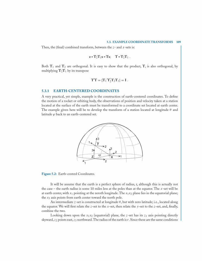
5.3. EXAMPLE COORDINATE TRANSFORMS 109
Then, the (final) combined transform, between the z- and x-sets is:
z = T2T1x = Tx; T = T2T1 .
Both T1 and T2 are orthogonal. It is easy to show that the product, T, is also orthogonal, bymultiplying T2T1 by its transpose
T′T = [T1′T′
2T2T1] = I .
5.3.1 EARTH-CENTERED COORDINATESA very practical, yet simple, example is the construction of earth-centered coordinates. To definethe motion of a rocket or orbiting body, the observations of position and velocity taken at a stationlocated at the surface of the earth must be transformed to a coordinate set located at earth center.The example given here will be to develop the transform of a station located at longitude θ andlatitude ϕ back to an earth-centered set.
Figure 5.2: Earth-centerd Coordinates.
It will be assume that the earth is a perfect sphere of radius, r, although this is actually notthe case – the earth radius is some 10 miles less at the poles than at the equator. The x-set will beat earth center, with x1 pointing at the zeroth longitude. The x1x2 plane lies in the equatorial plane;the x3 axis points from earth center toward the north pole.
An intermediate z-set is constructed at longitude θ , but with zero latitude; i.e., located alongthe equator. We will first relate the z-set to the x-set, then relate the y-set to the z-set, and, finally,combine the two.
Looking down upon the x1x2 (equatorial) plane, the z-set has its z1 axis pointing directlyskyward,z2 points east,z3 northward.The radius of the earth is r . Since these are the same conditions
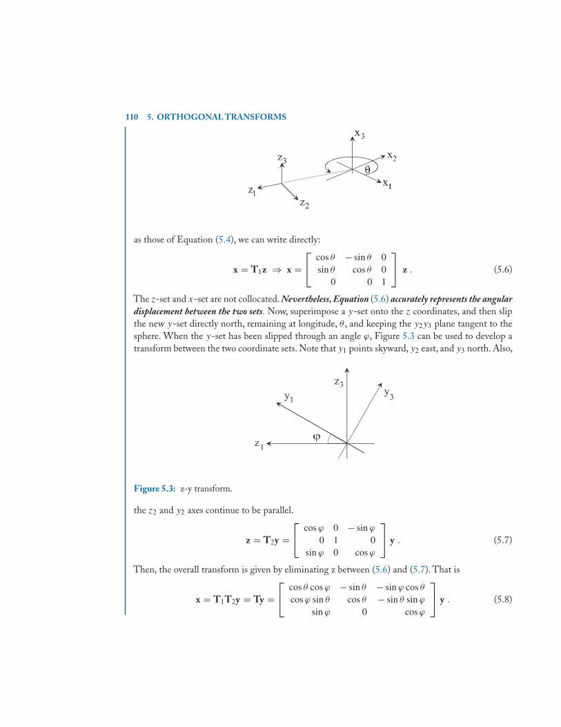
110 5. ORTHOGONAL TRANSFORMS
as those of Equation (5.4), we can write directly:
x = T1z ⇒ x =⎡⎣ cos θ − sin θ 0
sin θ cos θ 00 0 1
⎤⎦ z . (5.6)
The z-set and x-set are not collocated. Nevertheless, Equation (5.6) accurately represents the angulardisplacement between the two sets. Now, superimpose a y-set onto the z coordinates, and then slipthe new y-set directly north, remaining at longitude, θ , and keeping the y2y3 plane tangent to thesphere. When the y-set has been slipped through an angle ϕ, Figure 5.3 can be used to develop atransform between the two coordinate sets. Note that y1 points skyward, y2 east, and y3 north. Also,
Figure 5.3: z-y transform.
the z2 and y2 axes continue to be parallel.
z = T2y =⎡⎣ cos ϕ 0 − sin ϕ
0 1 0sin ϕ 0 cos ϕ
⎤⎦ y . (5.7)
Then, the overall transform is given by eliminating z between (5.6) and (5.7). That is
x = T1T2y = Ty =⎡⎣ cos θ cos ϕ − sin θ − sin ϕ cos θ
cos ϕ sin θ cos θ − sin θ sin ϕ
sin ϕ 0 cos ϕ
⎤⎦ y . (5.8)
5.3. EXAMPLE COORDINATE TRANSFORMS 111
Note that θ is measured eastward from zero degrees longitude to 360 degrees, not the usually givenEast Longitude and West Longitude (wherein θ is an angle between 0 and 180 degrees). In thismeasure, then, points in the United States will have θ values greater than 230 degrees. The latitudeis measured in the usual way, from zero degrees at the equator, to 90 degrees at the north pole.
The radius, r from earth center to the station, is given by {r, 0, 0}, measured in the y-set. Wetransform r into the x-set via T in (5.8). The result is:
rx =⎧⎨⎩
r cos θ cos ϕ
r sin θ cos ϕ
r sin ϕ
⎫⎬⎭ .
These are the well known polar coordinates of the vector. Note that although the y- and x-sets do nothave the same origin, vectors known in either set can be transformed to the other. More importantly,the above vector rx must be added to position vector observations taken at the station, (y-set) andthen transformed to the x-set. For example, radar data, taken from several stations is transformedfirst to a single station. This data defines, say, the instantaneous position of an orbiting body in itslocal coordinates. Its position relative to the inertial coordinates is rx plus the transformed positioninto the x-set. That is (with T taken from (5.8)):
px= [T]py + rx . (5.9)
The time derivative of (5.9) defines velocity. In cases wherein the rotation of the earth must be takeninto account, θ becomes a time dependent variable. Thus, the matrix T must be differentiated. Wewill consider the differentiation of a matrix in a later section.
As a check of the transform, T, plug all the y-set unit vectors, in turn, into (5.8).The results ineach case, of course, would be the columns of T – and the direction cosines of each of the y-set unitvectors, expressed in the x-set. For example, note that column 2 of T depends only upon θ . Thatdoes check: the unit vector {0, 1, 0}y is parallel to the x1x2 plane, and it projects onto that plane as{cos(90 + θ ), sin(90 + θ ), 0}. The point is that if this same reasoning had been used at the beginning,it would not have been necessary to develop an intermediate z-set. The transform (5.8) could bewritten directly. However, the reader should try this, and note that it is not easy. The 3 dimensionalthinking required is confusing, and prone to error. In most cases, it is safer and easier to developsuch transforms in a series of simple steps.
Sometimes, a rotation takes place about an axis that is not one of the coordinate axes givenin the problem. In that case, (as will be seen in the example problem, below), an intermediate set isset up specifically to orient the rotation about one of its coordinate axis. To do this, it is necessaryto take the cross product of two existing vectors to generate one of the coordinate axes in the new,rotated set. For this reason, we should first review this product (see also, Chapter 1, Section 1.2).
The “vector product,” or “cross product” of two vectors produces a vector which is orthogonalto both of the vectors crossed. In contrast, it will be recalled that the dot product of two vectorsproduces a scalar. The magnitude of the new vector is the product of the input vector magnitudes
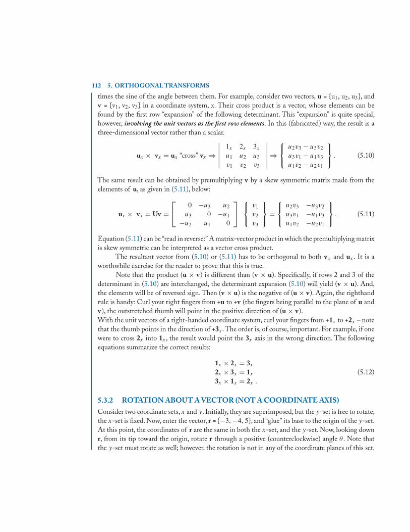
112 5. ORTHOGONAL TRANSFORMS
times the sine of the angle between them. For example, consider two vectors, u = {u1, u2, u3}, andv = {v1, v2, v3} in a coordinate system, x. Their cross product is a vector, whose elements can befound by the first row “expansion” of the following determinant. This “expansion” is quite special,however, involving the unit vectors as the first row elements. In this (fabricated) way, the result is athree-dimensional vector rather than a scalar.
ux × vx = ux “cross” vx ⇒∣∣∣∣∣∣
1x 2x 3x
u1 u2 u3
v1 v2 v3
∣∣∣∣∣∣ ⇒⎧⎨⎩
u2v3 − u3v2
u3v1 − u1v3
u1v2 − u2v1
⎫⎬⎭ . (5.10)
The same result can be obtained by premultiplying v by a skew symmetric matrix made from theelements of u, as given in (5.11), below:
ux × vx = Uv =⎡⎣ 0 −u3 u2
u3 0 −u1
−u2 u1 0
⎤⎦
⎧⎨⎩
v1
v2
v3
⎫⎬⎭ =
⎧⎨⎩
u2v3 −u3v2
u3v1 −u1v3
u1v2 −u2v1
⎫⎬⎭ . (5.11)
Equation (5.11) can be “read in reverse:” A matrix-vector product in which the premultiplying matrixis skew symmetric can be interpreted as a vector cross product.
The resultant vector from (5.10) or (5.11) has to be orthogonal to both vx and ux . It is aworthwhile exercise for the reader to prove that this is true.
Note that the product (u × v) is different than (v × u). Specifically, if rows 2 and 3 of thedeterminant in (5.10) are interchanged, the determinant expansion (5.10) will yield (v × u). And,the elements will be of reversed sign. Then (v × u) is the negative of (u × v). Again, the righthandrule is handy: Curl your right fingers from +u to +v (the fingers being parallel to the plane of u andv), the outstretched thumb will point in the positive direction of (u × v).With the unit vectors of a right-handed coordinate system, curl your fingers from +1x to +2x – notethat the thumb points in the direction of +3x . The order is, of course, important. For example, if onewere to cross 2x into 1x , the result would point the 3x axis in the wrong direction. The followingequations summarize the correct results:
1x × 2x = 3x
2x × 3x = 1x
3x × 1x = 2x .
(5.12)
5.3.2 ROTATION ABOUT A VECTOR (NOT A COORDINATE AXIS)Consider two coordinate sets, x and y. Initially, they are superimposed, but the y-set is free to rotate,the x-set is fixed. Now, enter the vector, r = {−3, −4, 5}, and “glue” its base to the origin of the y-set.At this point, the coordinates of r are the same in both the x-set, and the y-set. Now, looking downr, from its tip toward the origin, rotate r through a positive (counterclockwise) angle θ . Note thatthe y-set must rotate as well; however, the rotation is not in any of the coordinate planes of this set.
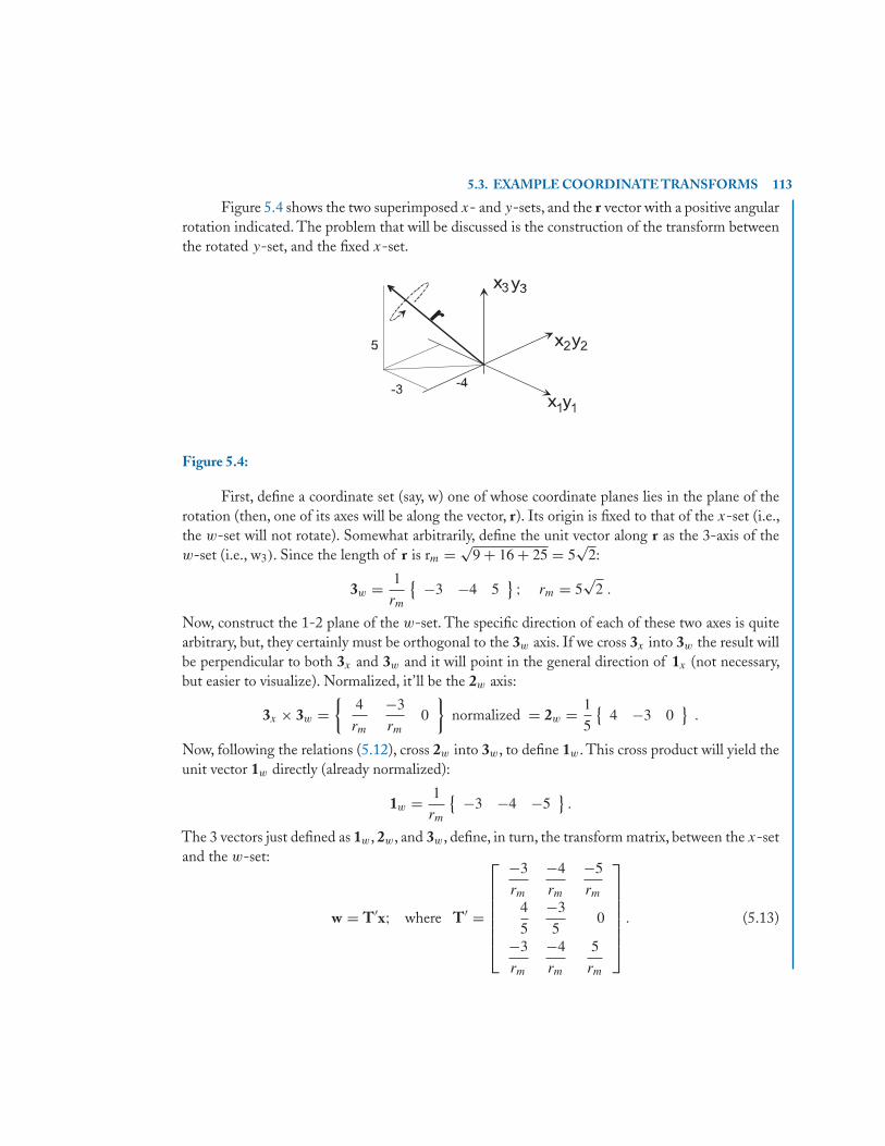
5.3. EXAMPLE COORDINATE TRANSFORMS 113
Figure 5.4 shows the two superimposed x- and y-sets, and the r vector with a positive angularrotation indicated. The problem that will be discussed is the construction of the transform betweenthe rotated y-set, and the fixed x-set.
Figure 5.4:
First, define a coordinate set (say, w) one of whose coordinate planes lies in the plane of therotation (then, one of its axes will be along the vector, r). Its origin is fixed to that of the x-set (i.e.,the w-set will not rotate). Somewhat arbitrarily, define the unit vector along r as the 3-axis of thew-set (i.e., w3). Since the length of r is rm = √
9 + 16 + 25 = 5√
2:
3w = 1
rm
{ −3 −4 5} ; rm = 5
√2 .
Now, construct the 1-2 plane of the w-set. The specific direction of each of these two axes is quitearbitrary, but, they certainly must be orthogonal to the 3w axis. If we cross 3x into 3w the result willbe perpendicular to both 3x and 3w and it will point in the general direction of 1x (not necessary,but easier to visualize). Normalized, it’ll be the 2w axis:
3x × 3w ={
4
rm
−3
rm0
}normalized = 2w = 1
5
{4 −3 0
}.
Now, following the relations (5.12), cross 2w into 3w, to define 1w. This cross product will yield theunit vector 1w directly (already normalized):
1w = 1
rm
{ −3 −4 −5}.
The 3 vectors just defined as 1w, 2w, and 3w, define, in turn, the transform matrix, between the x-setand the w-set:
w = T′x; where T′ =
⎡⎢⎢⎢⎢⎢⎢⎣
−3
rm
−4
rm
−5
rm4
5
−3
50
−3
rm
−4
rm
5
rm
⎤⎥⎥⎥⎥⎥⎥⎦
. (5.13)
114 5. ORTHOGONAL TRANSFORMS
That is, the 1st row of T′ is 1w, the second row is 2w, etc. To provide confidence that we have thetransform in the right order, put {−3, −4, 5} (the coordinates of r in the x set) into (5.13). Thesecoordinates will transform through (5.13) to a vector in the w-set with a w3 component equal to rm,and the w1 and w2 components equal to zero.
The inverse transform, x = Tw, is also determined by simply transposing the matrix T′.The 1-2 plane of the w-set is the plane of rotation. Note, however, that the w-set is not rotated.
Instead, we will define a new z-set, originally superimposed upon the w-set, but then rotated throughthe required θ angle. The transform between the w and z sets can be written directly, because it isthe same as that defined in Equation (5.4), above:
z = Qw ⇒ z =⎡⎣ cos θ − sin θ 0
sin θ cos θ 00 0 1
⎤⎦ w . (5.14)
Now that the transforms (5.13) and (5.14) are known, we can proceed with the solution to theproblem. Originally, before the rotation, the y-set and x-set are superimposed. Therefore, Equa-tion (5.13) holds for the y-set as well, and since before rotation the w- and z-sets are superimposed:
y = Tw = Tz (before rotation) . (5.15)
After the rotation, (5.13) still relates the x-set to the w-set because neither of them moves. Moreimportantly, (5.15) can still be used to relate the z-set to the y-set after rotation, because they movetogether:
y = Tz (after rotation) . (5.16)
Plugging the definition of (5.14) into (5.16):
y = TQw (5.17)
and since, from (5.13), w = T′x, the final transform is:
y = TQT′x (5.18)
and its inverse is (obviously):x = TQ′T′y . (5.19)
We have already seen that the transform of a vector, say x, is done through the premultiplication ofx by some matrix, T (y = Tx). Now, (5.19) implies that the rotational matrix, Q, is transformed byboth pre- and post multiplication (i.e., TQT′). And this is, indeed the general case – matrices aretransformed by pre- and post multiplication by the transforming matrices. This transformation of Qproduces the rotation given in Q, as observed in the x- and y-sets, respectively.
In (5.18), if we call the overall transform matrix W, then W = TQT′. The matrix W is the“transform” of Q. The transforming matrix, T, is orthogonal. In this case, as will be discussed in alater article, W and Q are said to be related by a “congruent” transform.
Section 5.4, below, discusses the transformation of matrices.
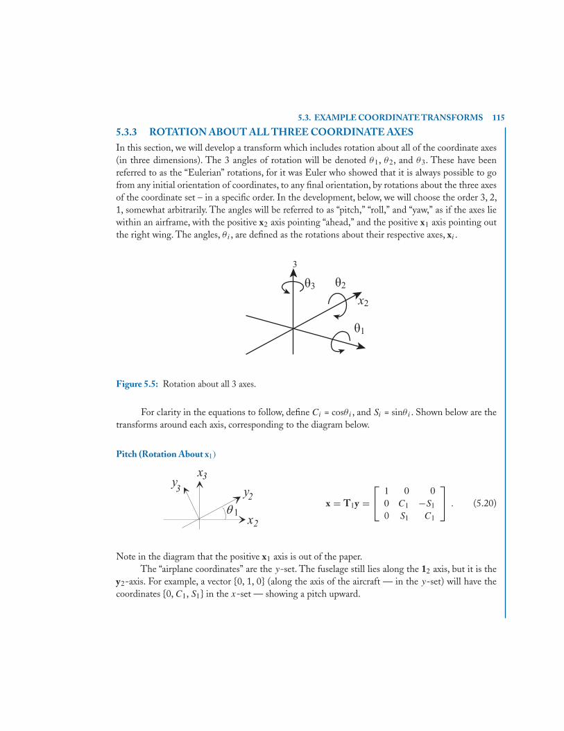
5.3. EXAMPLE COORDINATE TRANSFORMS 115
5.3.3 ROTATION ABOUT ALL THREE COORDINATE AXESIn this section, we will develop a transform which includes rotation about all of the coordinate axes(in three dimensions). The 3 angles of rotation will be denoted θ1, θ2, and θ3. These have beenreferred to as the “Eulerian” rotations, for it was Euler who showed that it is always possible to gofrom any initial orientation of coordinates, to any final orientation, by rotations about the three axesof the coordinate set – in a specific order. In the development, below, we will choose the order 3, 2,1, somewhat arbitrarily. The angles will be referred to as “pitch,” “roll,” and “yaw,” as if the axes liewithin an airframe, with the positive x2 axis pointing “ahead,” and the positive x1 axis pointing outthe right wing. The angles, θi , are defined as the rotations about their respective axes, xi .
Figure 5.5: Rotation about all 3 axes.
For clarity in the equations to follow, define Ci = cosθi , and Si = sinθi . Shown below are thetransforms around each axis, corresponding to the diagram below.
Pitch (Rotation About x1)
x = T1y =⎡⎣ 1 0 0
0 C1 −S1
0 S1 C1
⎤⎦ . (5.20)
Note in the diagram that the positive x1 axis is out of the paper.The “airplane coordinates” are the y-set. The fuselage still lies along the 12 axis, but it is the
y2-axis. For example, a vector {0, 1, 0} (along the axis of the aircraft — in the y-set) will have thecoordinates {0, C1, S1} in the x-set — showing a pitch upward.
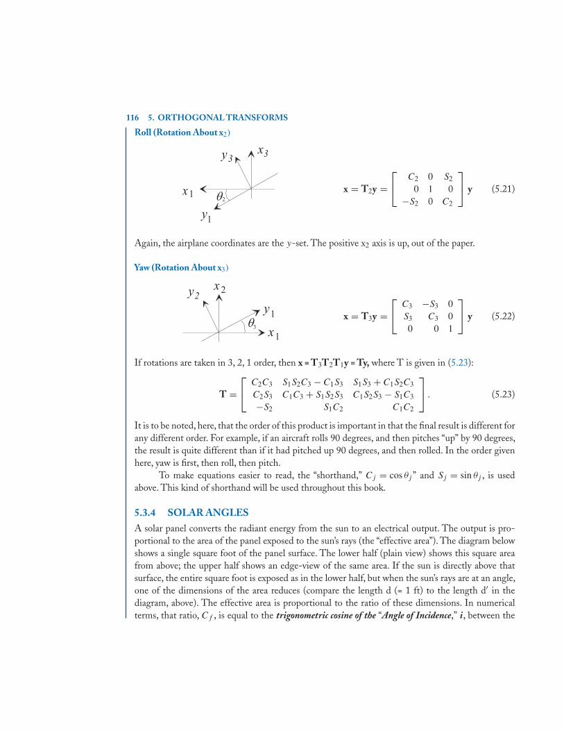
116 5. ORTHOGONAL TRANSFORMS
Roll (Rotation About x2)
x = T2y =⎡⎣ C2 0 S2
0 1 0−S2 0 C2
⎤⎦ y (5.21)
Again, the airplane coordinates are the y-set. The positive x2 axis is up, out of the paper.
Yaw (Rotation About x3)
x = T3y =⎡⎣ C3 −S3 0
S3 C3 00 0 1
⎤⎦ y (5.22)
If rotations are taken in 3, 2, 1 order, then x = T3T2T1y = Ty, where T is given in (5.23):
T =⎡⎣ C2C3 S1S2C3 − C1S3 S1S3 + C1S2C3
C2S3 C1C3 + S1S2S3 C1S2S3 − S1C3
−S2 S1C2 C1C2
⎤⎦ . (5.23)
It is to be noted, here, that the order of this product is important in that the final result is different forany different order. For example, if an aircraft rolls 90 degrees, and then pitches “up” by 90 degrees,the result is quite different than if it had pitched up 90 degrees, and then rolled. In the order givenhere, yaw is first, then roll, then pitch.
To make equations easier to read, the “shorthand,” Cj = cos θj ” and Sj = sin θj , is usedabove. This kind of shorthand will be used throughout this book.
5.3.4 SOLAR ANGLESA solar panel converts the radiant energy from the sun to an electrical output. The output is pro-portional to the area of the panel exposed to the sun’s rays (the “effective area”). The diagram belowshows a single square foot of the panel surface. The lower half (plain view) shows this square areafrom above; the upper half shows an edge-view of the same area. If the sun is directly above thatsurface, the entire square foot is exposed as in the lower half, but when the sun’s rays are at an angle,one of the dimensions of the area reduces (compare the length d (= 1 ft) to the length d′ in thediagram, above). The effective area is proportional to the ratio of these dimensions. In numericalterms, that ratio, Cf , is equal to the trigonometric cosine of the “Angle of Incidence,” i, between the
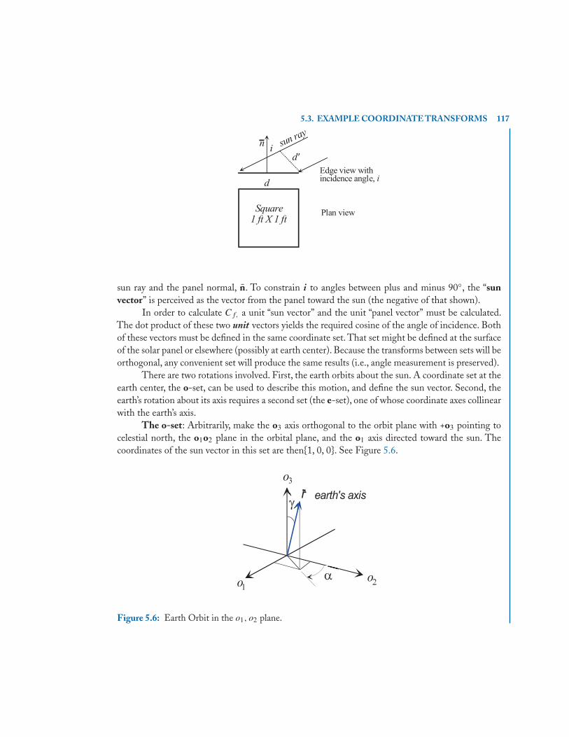
5.3. EXAMPLE COORDINATE TRANSFORMS 117
sun ray and the panel normal, n. To constrain i to angles between plus and minus 90◦, the “sunvector” is perceived as the vector from the panel toward the sun (the negative of that shown).
In order to calculate Cf, a unit “sun vector” and the unit “panel vector” must be calculated.The dot product of these two unit vectors yields the required cosine of the angle of incidence. Bothof these vectors must be defined in the same coordinate set. That set might be defined at the surfaceof the solar panel or elsewhere (possibly at earth center). Because the transforms between sets will beorthogonal, any convenient set will produce the same results (i.e., angle measurement is preserved).
There are two rotations involved. First, the earth orbits about the sun. A coordinate set at theearth center, the o-set, can be used to describe this motion, and define the sun vector. Second, theearth’s rotation about its axis requires a second set (the e-set), one of whose coordinate axes collinearwith the earth’s axis.
The o-set: Arbitrarily, make the o3 axis orthogonal to the orbit plane with +o3 pointing tocelestial north, the o1o2 plane in the orbital plane, and the o1 axis directed toward the sun. Thecoordinates of the sun vector in this set are then{1, 0, 0}. See Figure 5.6.
Figure 5.6: Earth Orbit in the o1, o2 plane.
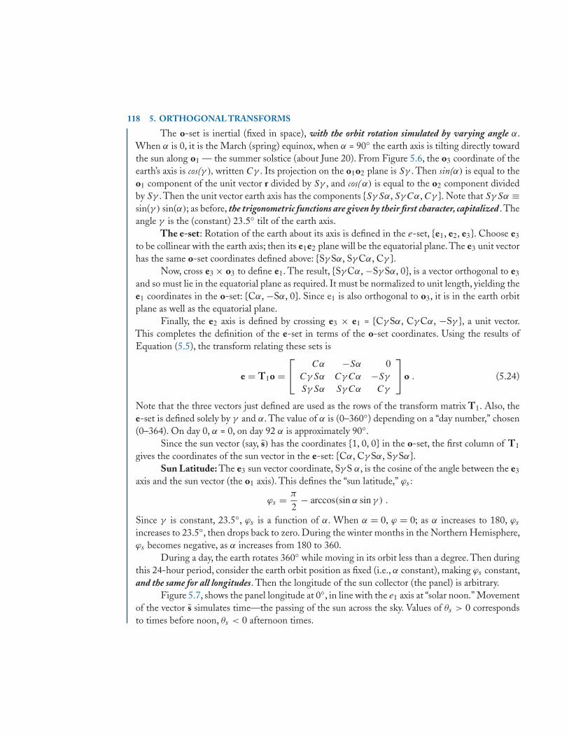
118 5. ORTHOGONAL TRANSFORMS
The o-set is inertial (fixed in space), with the orbit rotation simulated by varying angle α.When α is 0, it is the March (spring) equinox, when α = 90◦ the earth axis is tilting directly towardthe sun along o1 — the summer solstice (about June 20). From Figure 5.6, the o3 coordinate of theearth’s axis is cos(γ ), written Cγ . Its projection on the o1o2 plane is Sγ . Then sin(α) is equal to theo1 component of the unit vector r divided by Sγ , and cos(α) is equal to the o2 component dividedby Sγ . Then the unit vector earth axis has the components {Sγ Sα, SγCα, Cγ }. Note that Sγ Sα ≡sin(γ ) sin(α); as before, the trigonometric functions are given by their first character, capitalized . Theangle γ is the (constant) 23.5◦ tilt of the earth axis.
The e-set: Rotation of the earth about its axis is defined in the e-set, {e1, e2, e3}. Choose e3
to be collinear with the earth axis; then its e1e2 plane will be the equatorial plane. The e3 unit vectorhas the same o-set coordinates defined above: {Sγ Sα, Sγ Cα, Cγ }.
Now, cross e3 × o3 to define e1. The result, {Sγ Cα, −Sγ Sα, 0}, is a vector orthogonal to e3
and so must lie in the equatorial plane as required. It must be normalized to unit length, yielding thee1 coordinates in the o-set: {Cα, −Sα, 0}. Since e1 is also orthogonal to o3, it is in the earth orbitplane as well as the equatorial plane.
Finally, the e2 axis is defined by crossing e3 × e1 = {Cγ Sα, Cγ Cα, −Sγ }, a unit vector.This completes the definition of the e-set in terms of the o-set coordinates. Using the results ofEquation (5.5), the transform relating these sets is
e = T1o =⎡⎣ Cα −Sα 0
CγSα CγCα −Sγ
Sγ Sα SγCα Cγ
⎤⎦ o . (5.24)
Note that the three vectors just defined are used as the rows of the transform matrix T1. Also, thee-set is defined solely by γ and α. The value of α is (0–360◦) depending on a “day number,” chosen(0–364). On day 0, α = 0, on day 92 α is approximately 90◦.
Since the sun vector (say, s) has the coordinates {1, 0, 0} in the o-set, the first column of T1
gives the coordinates of the sun vector in the e-set: {Cα, Cγ Sα, Sγ Sα}.Sun Latitude: The e3 sun vector coordinate, Sγ S α, is the cosine of the angle between the e3
axis and the sun vector (the o1 axis). This defines the “sun latitude,” ϕs :
ϕs = π
2− arccos(sin α sin γ ) .
Since γ is constant, 23.5◦, ϕs is a function of α. When α = 0, ϕ = 0; as α increases to 180, ϕs
increases to 23.5◦, then drops back to zero. During the winter months in the Northern Hemisphere,ϕs becomes negative, as α increases from 180 to 360.
During a day, the earth rotates 360◦ while moving in its orbit less than a degree. Then duringthis 24-hour period, consider the earth orbit position as fixed (i.e., α constant), making ϕs constant,and the same for all longitudes. Then the longitude of the sun collector (the panel) is arbitrary.
Figure 5.7, shows the panel longitude at 0◦, in line with the e1 axis at “solar noon.” Movementof the vector s simulates time—the passing of the sun across the sky. Values of θs > 0 correspondsto times before noon, θs < 0 afternoon times.
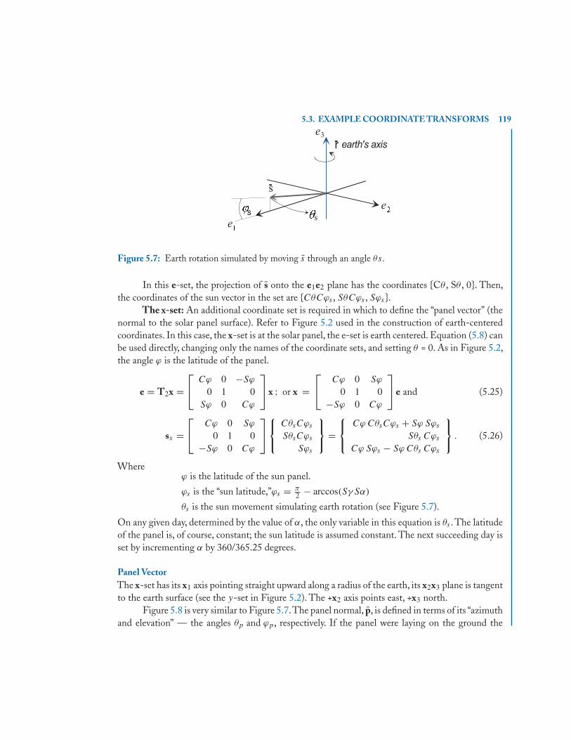
5.3. EXAMPLE COORDINATE TRANSFORMS 119
Figure 5.7: Earth rotation simulated by moving s through an angle θs.
In this e-set, the projection of s onto the e1e2 plane has the coordinates {Cθ , Sθ , 0}. Then,the coordinates of the sun vector in the set are {CθCϕs , SθCϕs , Sϕs}.
The x-set: An additional coordinate set is required in which to define the “panel vector” (thenormal to the solar panel surface). Refer to Figure 5.2 used in the construction of earth-centeredcoordinates. In this case, the x-set is at the solar panel, the e-set is earth centered. Equation (5.8) canbe used directly, changing only the names of the coordinate sets, and setting θ = 0. As in Figure 5.2,the angle ϕ is the latitude of the panel.
e = T2x =⎡⎣ Cϕ 0 −Sϕ
0 1 0Sϕ 0 Cϕ
⎤⎦ x ; or x =
⎡⎣ Cϕ 0 Sϕ
0 1 0−Sϕ 0 Cϕ
⎤⎦ e and (5.25)
sx =⎡⎣ Cϕ 0 Sϕ
0 1 0−Sϕ 0 Cϕ
⎤⎦⎧⎨⎩
CθsCϕs
SθsCϕs
Sϕs
⎫⎬⎭ =
⎧⎨⎩
Cϕ CθsCϕs + Sϕ Sϕs
Sθs Cϕs
Cϕ Sϕs − Sϕ Cθs Cϕs
⎫⎬⎭ . (5.26)
Whereϕ is the latitude of the sun panel.
ϕs is the “sun latitude,”ϕs = π2 − arccos(Sγ Sα)
θs is the sun movement simulating earth rotation (see Figure 5.7).
On any given day, determined by the value of α, the only variable in this equation is θs . The latitudeof the panel is, of course, constant; the sun latitude is assumed constant. The next succeeding day isset by incrementing α by 360/365.25 degrees.
Panel VectorThe x-set has its x1 axis pointing straight upward along a radius of the earth, its x2x3 plane is tangentto the earth surface (see the y-set in Figure 5.2). The +x2 axis points east, +x3 north.
Figure 5.8 is very similar to Figure 5.7.The panel normal, p, is defined in terms of its “azimuthand elevation” — the angles θp and ϕp, respectively. If the panel were laying on the ground the
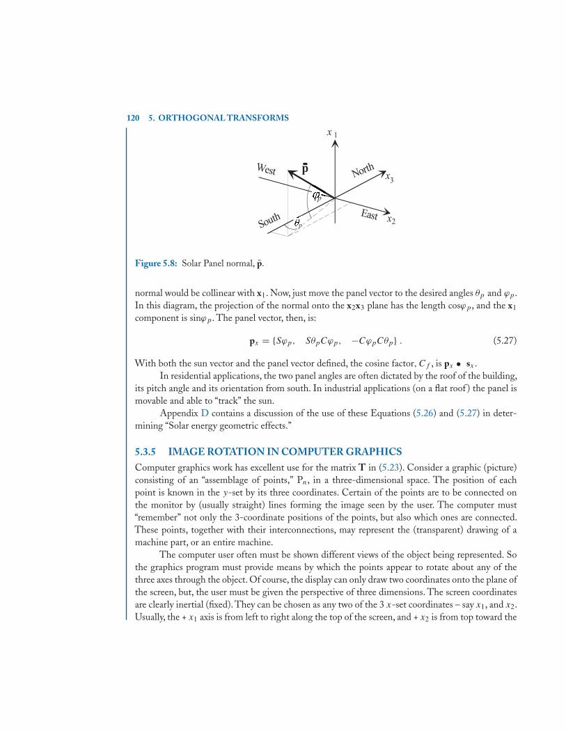
120 5. ORTHOGONAL TRANSFORMS
Figure 5.8: Solar Panel normal, p.
normal would be collinear with x1. Now, just move the panel vector to the desired angles θp and ϕp.In this diagram, the projection of the normal onto the x2x3 plane has the length cosϕp, and the x1
component is sinϕp. The panel vector, then, is:
px = {Sϕp, SθpCϕp, −CϕpCθp} . (5.27)
With both the sun vector and the panel vector defined, the cosine factor, Cf , is px • sx .In residential applications, the two panel angles are often dictated by the roof of the building,
its pitch angle and its orientation from south. In industrial applications (on a flat roof ) the panel ismovable and able to “track” the sun.
Appendix D contains a discussion of the use of these Equations (5.26) and (5.27) in deter-mining “Solar energy geometric effects.”
5.3.5 IMAGE ROTATION IN COMPUTER GRAPHICSComputer graphics work has excellent use for the matrix T in (5.23). Consider a graphic (picture)consisting of an “assemblage of points,” Pn, in a three-dimensional space. The position of eachpoint is known in the y-set by its three coordinates. Certain of the points are to be connected onthe monitor by (usually straight) lines forming the image seen by the user. The computer must“remember” not only the 3-coordinate positions of the points, but also which ones are connected.These points, together with their interconnections, may represent the (transparent) drawing of amachine part, or an entire machine.
The computer user often must be shown different views of the object being represented. Sothe graphics program must provide means by which the points appear to rotate about any of thethree axes through the object. Of course, the display can only draw two coordinates onto the plane ofthe screen, but, the user must be given the perspective of three dimensions. The screen coordinatesare clearly inertial (fixed). They can be chosen as any two of the 3 x-set coordinates – say x1, and x2.Usually, the + x1 axis is from left to right along the top of the screen, and + x2 is from top toward the
5.4. CONGRUENT AND SIMILARITY MATRIX TRANSFORMS 121
bottom of the display. The non-inertial y-set is located at the centroid of the object, and probablyat the center of the screen. In this case, then, the y-set is offset from the upper left corner of thescreen, to its center, by the amounts h0 (horizontal offset), and v0 (vertical offset). These offsets are1/2 the horizontal and vertical pixels of resolution of the screen.
When the command to rotate the object is given, the program uses equations like (5.23) toreposition the points and project them into computer screen coordinates. When the image is nextdisplayed, the same points (in their new positions) are interconnected by lines, and the image willappear to have rotated by the given angles.
If the image is required to appear to move, dynamically, the rotations must then be taken inincremental fashion. At each increment, the image must be erased, then rotated again, and redis-played – rapidly enough to give the impression of rotational motion at the screen. If the drawing iscomplicated, there will be many points, Pn. Since a vector multiplication is required for each point,plus reconnection of the points by lines, it can be seen that the computer must have a very large mainmemory, and be capable of high speed arithmetic (“floating point”) operations. It has only been inrecent years that such computers have been generally available.
Computer graphics software has become very complex. The above discussion omits all of thedrawing part, the interaction with the user — virtually all of the very difficult problems. But, thetransform matrix (5.23) is one of the many tools that make sophisticated graphics possible.
5.4 CONGRUENT AND SIMILARITY MATRIX TRANSFORMS
Earlier paragraphs have shown that a vector — a mathematical, and possibly physical, entity —can be viewed from different frames of reference, different coordinate sets. There is no particularsignificance to any given “frame,” and we can easily erect a different one to afford a better perspective.This is especially true for orthogonal reference frames which retain the vector length. The vectortransforms as easily as a single matrix-times-vector product.
The same can be said of a matrix, and functions of matrices. A matrix may be viewed from agiven reference set, or it can be transformed, along with the vectors upon which it may be operating,to a new set affording a more convenient view. It is of interest to see how a matrix is transformed.
Consider again the vector equation Ax= b. The coordinates in which A, x, and b are describedare quite arbitrary.Then, it may become necessary to transform these vectors using a (general) matrixP. The transform need not be an orthogonal one, so consider that P is a nonsingular matrix whoseinverse is P−1. Using P, we obtain:
x = Px and b = Pb (5.28)
in which x refers to the transformed vector x, and b refers to the transformed b. Of course, our maininterest is in the original matrix equation, and how b is obtained from x. Upon substitution of thetransform into the original equation Ax = b:
APx= Pb or P−1AP x = b . (5.29)
122 5. ORTHOGONAL TRANSFORMS
In the second Equation of (5.29) the matrix A is transformed to the new coordinates by combinedpre- and post-multiplication. The transform of A is:
A = P−1AP . (5.30)
The two matrices, A and A are said to be “similar” matrices, and the transform is called a “similaritytransform.” Since P and its inverse have reciprocal determinants, then (5.30) shows that A and Ahave the same determinant (i.e., |A| = |A|).
Now it will be shown that algebraic functions of A are transformed in the manner of (5.30),and thus, these functions are invariant under similarity transforms.
Matrix ProductThe product is transformed
AB ⇒ P−1APP−1BP = P−1(AB)P .
Matrix Addition/SubtractionA ± B ⇒ P−1AP ± P−1BP = P−1(A ± B)P .
Matrix InversionGiven that A =P−1AP, then by the inversion of a product rule: A−1 = P−1A−1P.
Then, all these operations transform just as A itself transforms — these operations remaininvariant under similarity transformation.
Matrix TranspositionThis case is somewhat different.
Given A = P−1AP, by transposition of a product: A′ = P′A′[P−1]′.This is not the same as thetransformation of A unless P is orthogonal. If the matrix, P, is not orthogonal then the operationof transposition is not invariant under transformation.
Three out of four isn’t bad. Functions of matrices which involve addition/subtraction, multi-plication, and inversion, remain invariant under similarity transformation:
f (A, B, C, , , A−1, B−1, C−1) ⇔ f (A, B, C, , , A−1, B−1, C−1) .
That is, a given function of matrices “implies” the same function of the same matrices, transformedto some new coordinate system by a similarity transform, as long as the function includes just thoseoperations which passed the above test. For example, a given polynomial in A:
c0An + c1An−1 + c2An−2 + · · · + cn−1A + cnI = 0
implies the same polynomial, with the same coefficients, in the transformed matrix A.
5.5. DIFFERENTIATION OF MATRICES, ANGULAR VELOCITY 123
If the transforming matrix is orthogonal, the transform is called “congruent,” and as describedearlier, the invariant functions will include transposition. Further, if A -A′ = 0, the matrix is sym-metric. Since the subtraction is invariant under congruent transformation then symmetric matricesremain symmetric under such transformation.
5.5 DIFFERENTIATION OF MATRICES, ANGULARVELOCITY
The objectives of this section will be to define the derivative of a matrix whose elements are variablefunctions, and then to use this definition in the development of the angular velocity matrix. Ofcourse, angular velocity is a vector quantity. It was shown earlier that the vector cross product can beaffected by the product of a 3X3 skew-symmetric matrix elements times a 3X1 vector. In fact, thisis just how the angular velocity vector emerges in this development.
Suppose the elements of the matrix A are functions of a scalar variable, t. Then:
A(t) = [aij (t)] .
Now, if t is incremented by dt, note that each element of A is incremented – that is
A(t + dt) = [aij (t + dt)] .
Then, if the original A matrix is subtracted, the result divided by dt, and the limit taken as dtapproaches zero, we see that the overall result is
d
dt[A(t)] =
[daij (t)
dt
]. (5.31)
That is, the differentiation of A is accomplished by differentiating each element of A. Now, con-sidering the variable to be time, t, we denote the time derivative as
d
dtA(t) ≡ A ≡ At . (5.32)
Notice the unusual notation At for the derivative of A. We can define the following derivatives:
d
dt[A + B] = A + B = At + Bt and (5.33)
d
dt[AB] = AB + AB = At B + ABt . (5.34)
The results (5.33) and (5.34) are just like their scalar counterparts. However, in (5.34), the originalproduct order, AB, must be maintained in the derivative of the product. Of course, if more than twomatrices are involved in the product then
[ABC]t = At [BC] + A[BC]t = At BC + ABt C + ABCt

124 5. ORTHOGONAL TRANSFORMS
and again the order of the product is maintained.The derivative of A−1 can be found by noting that
AA−1 = I thenAA−1 + AA−1 = 0A−1 = −A−1AA−1 .
5.5.1 VELOCITY OF A POINT ON A WHEELA point, p, rides on the periphery of a wheel (or disk), as shown in Figure 5.9. The axis of the wheelis attached to a shaft (in the plane of the paper) which is also capable of rotation.
As in previous examples, intermediate coordinate sets are used, with each one describing oneangular displacement (and velocity) about one of its axes. In this case, the angles are θ2 and θ3.
Figure 5.9:
An inertial (fixed) x-set is set up at the point “O” in the figure, with axes as shown (the +x3
axis is up, out of the paper). A y-set is constructed, also at point O, which rotates about its y2 axis(collinear with x2). This rotation angle is denoted θ2. Lastly, a z-set is constructed at point O, whichrotates with angle θ3 about the y3, z3 axes.
As observed in the z-set, the point p is fixed, with coordinates {rp, 0, 0}; and note that thepoint p does remain at a constant distance from point O—equal to the radius of the disk. That is,all the motion is angular rotation.
To find the velocity of the point p, the vector rx must first be found. Its time derivative is thevelocity of p. To find rx , vector rz is transformed from the z-set to the x-set. The two transforms
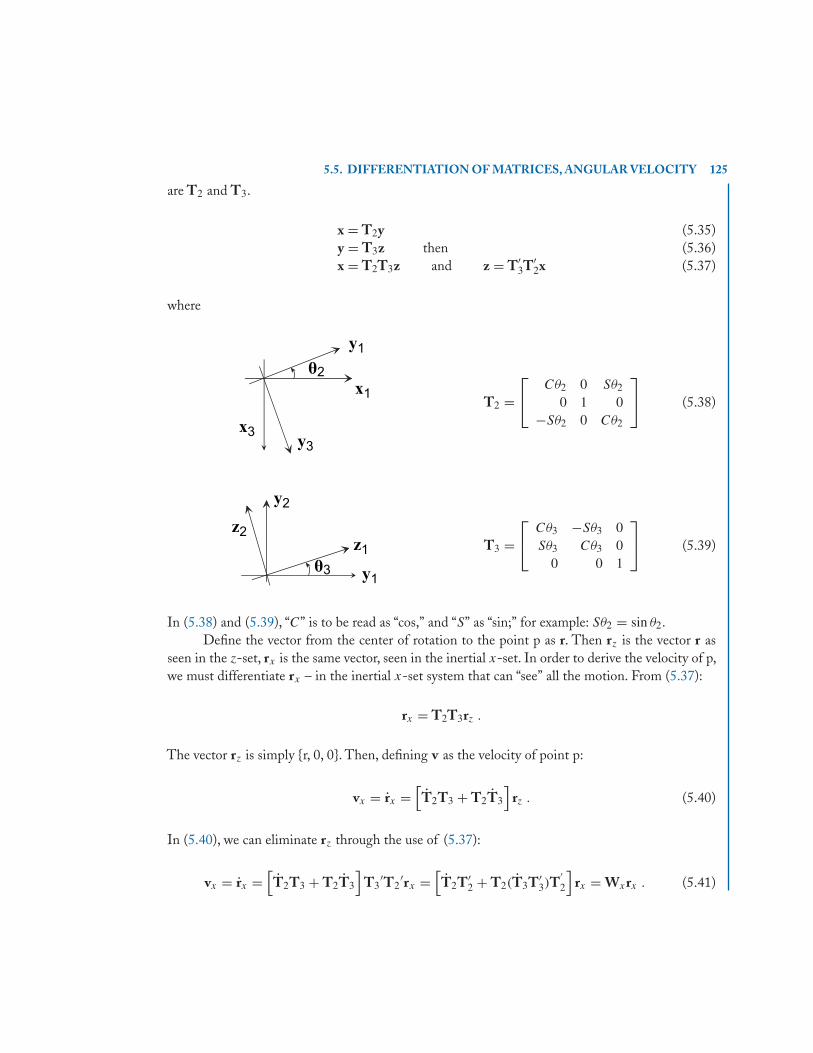
5.5. DIFFERENTIATION OF MATRICES, ANGULAR VELOCITY 125
are T2 and T3.
x = T2y (5.35)y = T3z then (5.36)x = T2T3z and z = T′
3T′2x (5.37)
where
T2 =⎡⎣ Cθ2 0 Sθ2
0 1 0−Sθ2 0 Cθ2
⎤⎦ (5.38)
T3 =⎡⎣ Cθ3 −Sθ3 0
Sθ3 Cθ3 00 0 1
⎤⎦ (5.39)
In (5.38) and (5.39), “C” is to be read as “cos,” and “S” as “sin;” for example: Sθ2 = sin θ2.Define the vector from the center of rotation to the point p as r. Then rz is the vector r as
seen in the z-set, rx is the same vector, seen in the inertial x-set. In order to derive the velocity of p,we must differentiate rx – in the inertial x-set system that can “see” all the motion. From (5.37):
rx = T2T3rz .
The vector rz is simply {r, 0, 0}. Then, defining v as the velocity of point p:
vx = rx =[
T2T3 + T2T3
]rz . (5.40)
In (5.40), we can eliminate rz through the use of (5.37):
vx = rx =[
T2T3 + T2T3
]T3
′T2′rx =
[T2T′
2 + T2(T3T′3)T
′2
]rx = Wxrx . (5.41)
126 5. ORTHOGONAL TRANSFORMS
In (5.41) the two important products are:
T2T2′ = θ2
⎡⎣ −Sθ2 0 Cθ2
0 0 0−Cθ2 0 −Sθ2
⎤⎦⎡⎣ Cθ2 0 −Sθ2
0 1 0Sθ2 0 Cθ2
⎤⎦ =
⎡⎣ 0 0 θ2
0 0 0−θ2 0 0
⎤⎦ and
T3T3′ = θ3
⎡⎣ −Sθ3 −Cθ3 0
Cθ3 −Sθ3 00 0 0
⎤⎦⎡⎣ Cθ3 Sθ3 0
−Sθ3 Cθ3 00 0 1
⎤⎦ =
⎡⎣ 0 −θ3 0
θ3 0 00 0 0
⎤⎦
where, again, S means sine (e.g., Sθ2 = sin θ2), and C means cosine.It should be clear that the elements of angular velocity are emerging in the products of these
Tj Tj′ matrices. That is, if Tj is the transform matrix defining rotation about the jth (inertial)
axis, then Tj Tj′ provides the j th component of angular velocity. Also, in (5.41), note that the
components of rotation about the 3-axis must be transformed back to the inertial x-set, while therotation about the 2-axis is already described in the x-set, and need not be transformed. Note againthat the transform af a matrix is accomplished by pre- and postmultiplying matrices. Specifically, inthe Wx matrix, the components, T3T3
′, must be transformed, while those from T2T2′ do not.
Wx = T2T2′ + T2(T3T3
′)T2′ . (5.42)
Angular velocity matrices which “emerge” in this way are always “skew symmetric.” That is
W = −W′ =⎡⎣ 0 −ω3 ω2
ω3 0 −ω1
−ω2 ω1 0
⎤⎦ . (5.43)
In the general case, with the transform T = T1T2T3, (rotation about all three coordinate axes) theangular velocity matrix would be:
Wx = T1T1′ + T1(T2T2
′)T1′ + T1T2(T3T3
′)T2′T1
′ .
And, again note the transformation of the 2-axis and 3-axis angular velocity components.In the example problem of Figure 5.9, multiplying the terms out in (5.42)
Wx = T2T2′ + T2(T3T3
′)T2′ =
⎡⎣ 0 −Cθ2θ3 θ2
Cθ2θ3 0 −Sθ2θ3
−θ2 Sθ2θ3 0
⎤⎦ . (5.44)
Therefore, the angular velocity (vector quantity) for the problem is:
ωωωx =⎧⎨⎩
ω1
ω2
ω3
⎫⎬⎭ =
⎧⎨⎩
θ3 sin θ2
θ2
θ3 cos θ2
⎫⎬⎭ . (5.45)
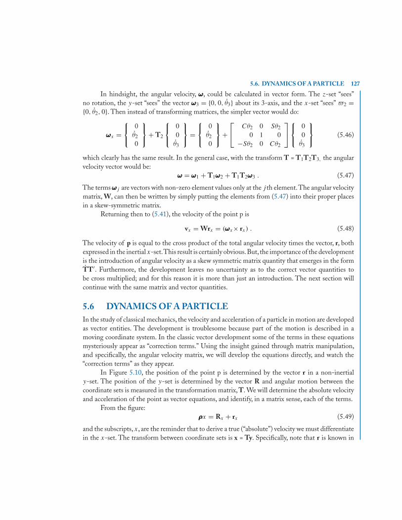
5.6. DYNAMICS OF A PARTICLE 127
In hindsight, the angular velocity, ωωω, could be calculated in vector form. The z-set “sees”no rotation, the y-set “sees” the vector ωωω3 = {0, 0, θ3} about its 3-axis, and the x-set “sees” �2 ={0, θ2, 0}. Then instead of transforming matrices, the simpler vector would do:
ωωωx =⎧⎨⎩
0θ2
0
⎫⎬⎭+ T2
⎧⎨⎩
00
θ3
⎫⎬⎭ =
⎧⎨⎩
0θ2
0
⎫⎬⎭+
⎡⎣ Cθ2 0 Sθ2
0 1 0−Sθ2 0 Cθ2
⎤⎦⎧⎨⎩
00
θ3
⎫⎬⎭ (5.46)
which clearly has the same result. In the general case, with the transform T = T1T2T3, the angularvelocity vector would be:
ωωω = ωωω1 + T1ωωω2 + T1T2ωωω3 . (5.47)
The terms ωωωj are vectors with non-zero element values only at the j th element.The angular velocitymatrix, W, can then be written by simply putting the elements from (5.47) into their proper placesin a skew-symmetric matrix.
Returning then to (5.41), the velocity of the point p is
vx = Wrx = (ωωωx× rx) . (5.48)
The velocity of p is equal to the cross product of the total angular velocity times the vector, r, bothexpressed in the inertial x-set.This result is certainly obvious.But, the importance of the developmentis the introduction of angular velocity as a skew symmetric matrix quantity that emerges in the formTT′. Furthermore, the development leaves no uncertainty as to the correct vector quantities tobe cross multiplied; and for this reason it is more than just an introduction. The next section willcontinue with the same matrix and vector quantities.
5.6 DYNAMICS OF A PARTICLEIn the study of classical mechanics, the velocity and acceleration of a particle in motion are developedas vector entities. The development is troublesome because part of the motion is described in amoving coordinate system. In the classic vector development some of the terms in these equationsmysteriously appear as “correction terms.” Using the insight gained through matrix manipulation,and specifically, the angular velocity matrix, we will develop the equations directly, and watch the“correction terms” as they appear.
In Figure 5.10, the position of the point p is determined by the vector r in a non-inertialy-set. The position of the y-set is determined by the vector R and angular motion between thecoordinate sets is measured in the transformation matrix, T. We will determine the absolute velocityand acceleration of the point as vector equations, and identify, in a matrix sense, each of the terms.
From the figure:ρρρx = Rx + rx (5.49)
and the subscripts, x, are the reminder that to derive a true (“absolute”) velocity we must differentiatein the x-set. The transform between coordinate sets is x = Ty. Specifically, note that r is known in
128 5. ORTHOGONAL TRANSFORMS
Figure 5.10: Particle Dynamics.
the y-set and must be transformed as rx = Try in (5.49). Then, by differentiation:
ρx = Rx + Try+Tryρx = Rx + Try + TT′rx = Rx + Try + (ωωωx× rx) . (5.50)ρx = Rx+
{ry}
x + (ωωω × rx) (5.51)
which is the absolute velocity of the point p, expressed in the x-set. The (�× r) term emerges thesame way that it did in the last section: TT′ is W, and note that W is Wx . The notation
{ry}x
isused to emphasize that the derivative of ry is taken, and the results then transformed to the x-set(not the derivative of rx). The derivative of ry is usually referred to as the “apparent velocity.” It isthe velocity that would be measured without any knowledge that the y-set is not inertial. Note thatthis matrix development is straightforward and leaves no question as to which coordinate set thevectors are to be defined in.
Often, it is desired to express the absolute velocity in the non-inertial set. This can be doneby simply transforming ρx to the y-set. However, it is interesting to start back at the first of (5.50),and to consider the transform of the angular velocity:
Wy = T′WxT (5.52)but Wx = TT′
then Wy = T′TT′T = T′T . (5.53)
Now, returning to (5.50)
{ρx}y = T′Rx + ry+T′Try{ρx}y = {Rx}y + ry + Wyry{ρx}y = {Rx}y + ry + (ωωωy × ry)
(5.54)
5.6. DYNAMICS OF A PARTICLE 129
which is the absolute velocity of p, expressed in the y-set. Note the similarity to (5.51).Now, for the acceleration, we must differentiate the first (5.50) equation:
ρx = Rx + Try + Try + Try+Tryρx = Rx + Try + 2TT′{ry}x+TT′rxρx = Rx + {ry}x + 2[Wx]{ry}x + TT′rx .
(5.55)
In (5.55), note the new correction term consisting of the angular velocity crossed into the “apparentvelocity” transformed to the x-set. But, to interpret further, consider the definition TT′ = Wx . Bydifferentiation:
d
dt[TT′] = TT′ + TT′ = Wx ; then TT′ = Wx − TT′ .
Since the angular velocity matrix is skew symmetric:
TT′ = Wx = −W′x = −TT′
then W2x = [TT′][−TT′] = −TT′
finally TT′ = Wx + W2x .
Then, taking this back to (5.55):
ρx = Rx + {ry}x + 2[Wx]{ry}x + TT′rxρx = Rx + {ry}x + 2[Wx]{ry}x + [Wx + W2
x ]rx (5.56)ρρρx = Rx + {ry}x + 2(ωωωx × {ry}x) + (ωωωx × rx) + ωωωx × (ωωωx × rx) (5.57)
both (5.56) and (5.57) show the final result for the absolute acceleration. The vector form, (5.57),is the form most often seen. Note that W2r = WWr is simply the cross product of a cross product,shown as the final term of (5.57).The absolute acceleration, then, has three cross product “correctionterms.” This also shows that when parts of the total motion of the particle are described in a non-inertial coordinate set, the equations of motion can become somewhat complicated.
This absolute acceleration is transformed to the y-set in the same way that velocity is trans-formed. This time, however, we must transform W2.
T′W2xT = [T′WxT][T′WxT] = W2
y (5.58)
which shows that the square of Wx (or, in fact, any integer power of Wx) transforms just like Wx .Then, basically we must transform the equation:
ρx = Rx + Try + 2[Wx]{ry}x + [Wx + W2x ]rx .
The transformation is accomplished by premultiplying the above equation by T′. Then:
{ρx}y = {Rx}y + ry + 2T′WxTry + T′[Wx + W2x ]Try
{ρx}y = {Rx}y + ry + 2[Wy]{ry} + [Wy + W2y ]ry (5.59)
{ρρρx}y = {Rx}y + ry + 2(ωωωy × ry) + (ωωωy × ry) + ωωωy × (ωωωy × ry) . (5.60)
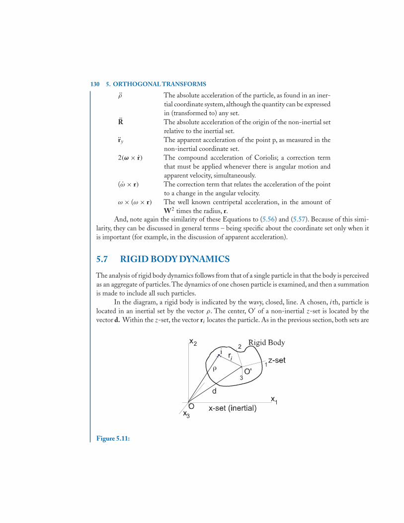
130 5. ORTHOGONAL TRANSFORMS
ρ The absolute acceleration of the particle, as found in an iner-tial coordinate system, although the quantity can be expressedin (transformed to) any set.
R The absolute acceleration of the origin of the non-inertial setrelative to the inertial set.
ry The apparent acceleration of the point p, as measured in thenon-inertial coordinate set.
2(ω × r) The compound acceleration of Coriolis; a correction termthat must be applied whenever there is angular motion andapparent velocity, simultaneously.
(ω × r) The correction term that relates the acceleration of the pointto a change in the angular velocity.
ω × (ω × r) The well known centripetal acceleration, in the amount ofW2 times the radius, r.
And, note again the similarity of these Equations to (5.56) and (5.57). Because of this simi-larity, they can be discussed in general terms – being specific about the coordinate set only when itis important (for example, in the discussion of apparent acceleration).
5.7 RIGID BODY DYNAMICS
The analysis of rigid body dynamics follows from that of a single particle in that the body is perceivedas an aggregate of particles.The dynamics of one chosen particle is examined, and then a summationis made to include all such particles.
In the diagram, a rigid body is indicated by the wavy, closed, line. A chosen, ith, particle islocated in an inertial set by the vector ρ. The center, O′ of a non-inertial z-set is located by thevector d. Within the z-set, the vector ri locates the particle. As in the previous section, both sets are
Figure 5.11:
5.7. RIGID BODY DYNAMICS 131
required because the z-set is often the one in which the particle is observed, but the x-set is requiredin which to do the differentiation necessary in the use of Newton’s second law. Since the ith is justone of the particles, the vectors r and ρ must be given subscripts:
ρi = d + ri . (5.61)
Using Newton’s second law for the ith particle:
Fi = miρi . (5.62)
WhereFi is the total force applied to the particlemi is the mass of the particle, andρi is its absolute acceleration.
The force on the particle is the result of both internal forces, f ij , from the adjoining particles (twosubscripts), and the external applied force, f i (one subscript). Then Fi = fij + fi .
Making the substitutions for Fi and for ρi , the equation of equilibrium is obtained by summingover all the particles in the system (rigid body):∑
i
fij +∑
i
fi =∑
i
mi(d + ri ) . (5.63)
Since the particles do not move relative to one another within the rigid body, each f ij must beaccompanied by an equal but opposite force, f ji . Then the sum of forces f ij must be zero. The sumof f i is simply the external force vector, f on the body. Also, in (5.63), the vector d is independentof which particle is chosen, so the sum is just that of the particle masses:
f = md +∑
i
mi ri where m is the total mass of the rigid body. (5.64)
An important simplification results if the mass points are located in relation to the center of gravityof the body. This is accomplished in the figure by redefining ri :
ri = rc + (ri )c . (5.65)
In (5.65), rc is a fixed vector from the origin O′ to the center of gravity, cg. The new vector (ri )c
emanates from the cg and terminates at the ith mass point. Then∑i
mi ri =∑
i
mi rc +∑
i
mi(ri )c . (5.66)
By definition of the center of gravity, the last term in (5.66) is zero. Thus,
f = md + mrc = m(d + rc) . (5.67)
The motion of translation can be determined by treating the rigid body as a single particle, with thetotal mass located at its center of gravity.
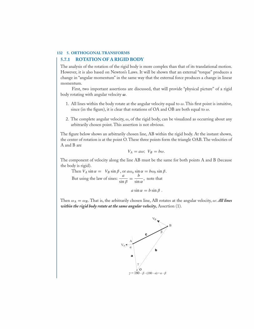
132 5. ORTHOGONAL TRANSFORMS
5.7.1 ROTATION OF A RIGID BODYThe analysis of the rotation of the rigid body is more complex than that of its translational motion.However, it is also based on Newton’s Laws. It will be shown that an external “torque” produces achange in “angular momentum” in the same way that the external force produces a change in linearmomentum.
First, two important assertions are discussed, that will provide “physical picture” of a rigidbody rotating with angular velocity ω.
1. All lines within the body rotate at the angular velocity equal to ω. This first point is intuitive,since (in the figure), it is clear that rotations of OA and OB are both equal to ω.
2. The complete angular velocity, ω, of the rigid body, can be visualized as occurring about anyarbitrarily chosen point. This assertion is not obvious.
The figure below shows an arbitrarily chosen line, AB within the rigid body. At the instant shown,the center of rotation is at the point O. These three points form the triangle OAB. The velocities ofA and B are
VA = aω; VB = bω.
The component of velocity along the line AB must be the same for both points A and B (becausethe body is rigid).
Then VA sin α = VB sin β , or aωa sin α = bωb sin β.
But using the law of sines:a
sin β= b
sin α, note that
a sin α = b sin β .
Then ωA = ωB . That is, the arbitrarily chosen line, AB rotates at the angular velocity, ω: All lineswithin the rigid body rotate at the same angular velocity, Assertion (1).
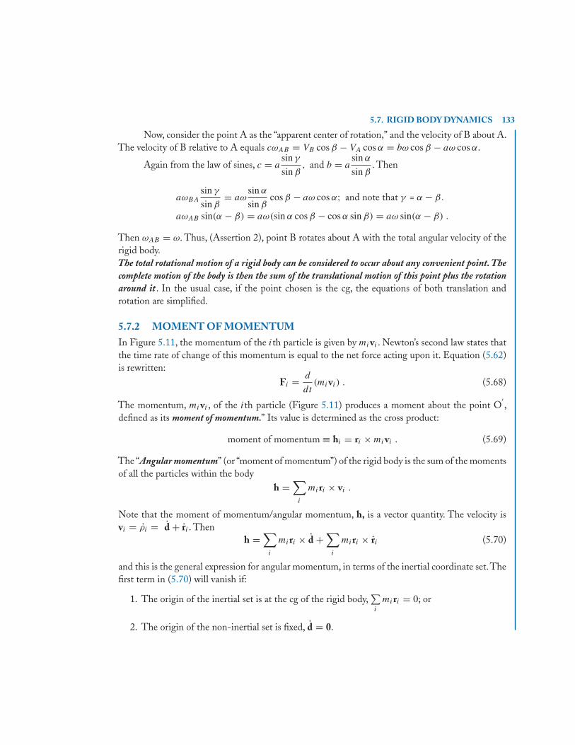
5.7. RIGID BODY DYNAMICS 133
Now, consider the point A as the “apparent center of rotation,” and the velocity of B about A.The velocity of B relative to A equals cωAB = VB cos β − VA cos α = bω cos β − aω cos α.
Again from the law of sines, c = asin γ
sin β, and b = a
sin α
sin β. Then
aωBA
sin γ
sin β= aω
sin α
sin βcos β − aω cos α; and note that γ = α − β.
aωAB sin(α − β) = aω(sin α cos β − cos α sin β) = aω sin(α − β) .
Then ωAB = ω. Thus, (Assertion 2), point B rotates about A with the total angular velocity of therigid body.The total rotational motion of a rigid body can be considered to occur about any convenient point. Thecomplete motion of the body is then the sum of the translational motion of this point plus the rotationaround it . In the usual case, if the point chosen is the cg, the equations of both translation androtation are simplified.
5.7.2 MOMENT OF MOMENTUMIn Figure 5.11, the momentum of the ith particle is given by mivi . Newton’s second law states thatthe time rate of change of this momentum is equal to the net force acting upon it. Equation (5.62)is rewritten:
Fi = d
dt(mivi ) . (5.68)
The momentum, mivi , of the ith particle (Figure 5.11) produces a moment about the point O′,
defined as its moment of momentum.” Its value is determined as the cross product:
moment of momentum ≡ hi = ri × mivi . (5.69)
The “Angular momentum” (or “moment of momentum”) of the rigid body is the sum of the momentsof all the particles within the body
h =∑
i
miri × vi .
Note that the moment of momentum/angular momentum, h, is a vector quantity. The velocity isvi = ρi = d + ri . Then
h =∑
i
miri × d +∑
i
miri × ri (5.70)
and this is the general expression for angular momentum, in terms of the inertial coordinate set.Thefirst term in (5.70) will vanish if:
1. The origin of the inertial set is at the cg of the rigid body,∑i
miri = 0; or
2. The origin of the non-inertial set is fixed, d = 0.
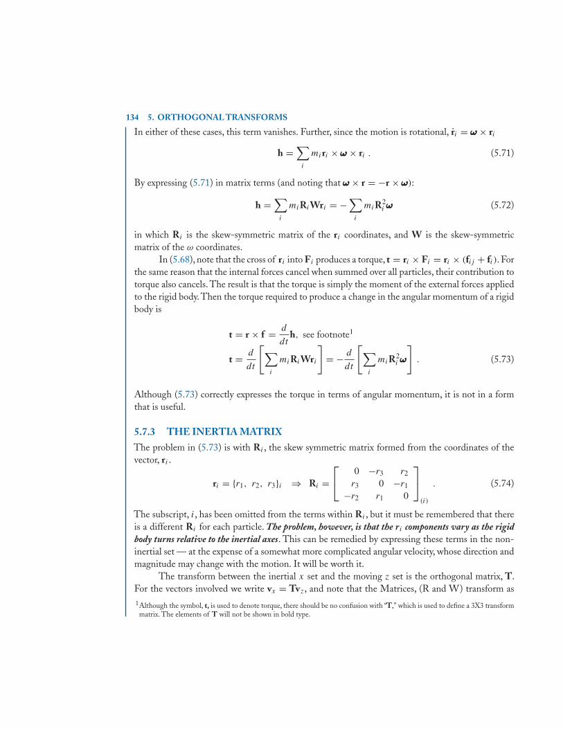
134 5. ORTHOGONAL TRANSFORMS
In either of these cases, this term vanishes. Further, since the motion is rotational, ri = ωωω × ri
h =∑
i
miri × ωωω × ri . (5.71)
By expressing (5.71) in matrix terms (and noting that ωωω × r = −r × ωωω):
h =∑
i
miRiWri = −∑
i
miR2i ωωω (5.72)
in which Ri is the skew-symmetric matrix of the ri coordinates, and W is the skew-symmetricmatrix of the ω coordinates.
In (5.68), note that the cross of ri into Fi produces a torque, t = ri × Fi = ri × (fij + fi ). Forthe same reason that the internal forces cancel when summed over all particles, their contribution totorque also cancels. The result is that the torque is simply the moment of the external forces appliedto the rigid body. Then the torque required to produce a change in the angular momentum of a rigidbody is
t = r × f = d
dth, see footnote1
t = d
dt
[∑i
miRiWri
]= − d
dt
[∑i
miR2i ωωω
]. (5.73)
Although (5.73) correctly expresses the torque in terms of angular momentum, it is not in a formthat is useful.
5.7.3 THE INERTIA MATRIXThe problem in (5.73) is with Ri , the skew symmetric matrix formed from the coordinates of thevector, ri .
ri = {r1, r2, r3}i ⇒ Ri =⎡⎣ 0 −r3 r2
r3 0 −r1
−r2 r1 0
⎤⎦
(i)
. (5.74)
The subscript, i, has been omitted from the terms within Ri , but it must be remembered that thereis a different Ri for each particle. The problem, however, is that the ri components vary as the rigidbody turns relative to the inertial axes. This can be remedied by expressing these terms in the non-inertial set — at the expense of a somewhat more complicated angular velocity, whose direction andmagnitude may change with the motion. It will be worth it.
The transform between the inertial x set and the moving z set is the orthogonal matrix, T.For the vectors involved we write vx = Tvz, and note that the Matrices, (R and W) transform as1Although the symbol, t, is used to denote torque, there should be no confusion with “T,” which is used to define a 3X3 transformmatrix. The elements of T will not be shown in bold type.
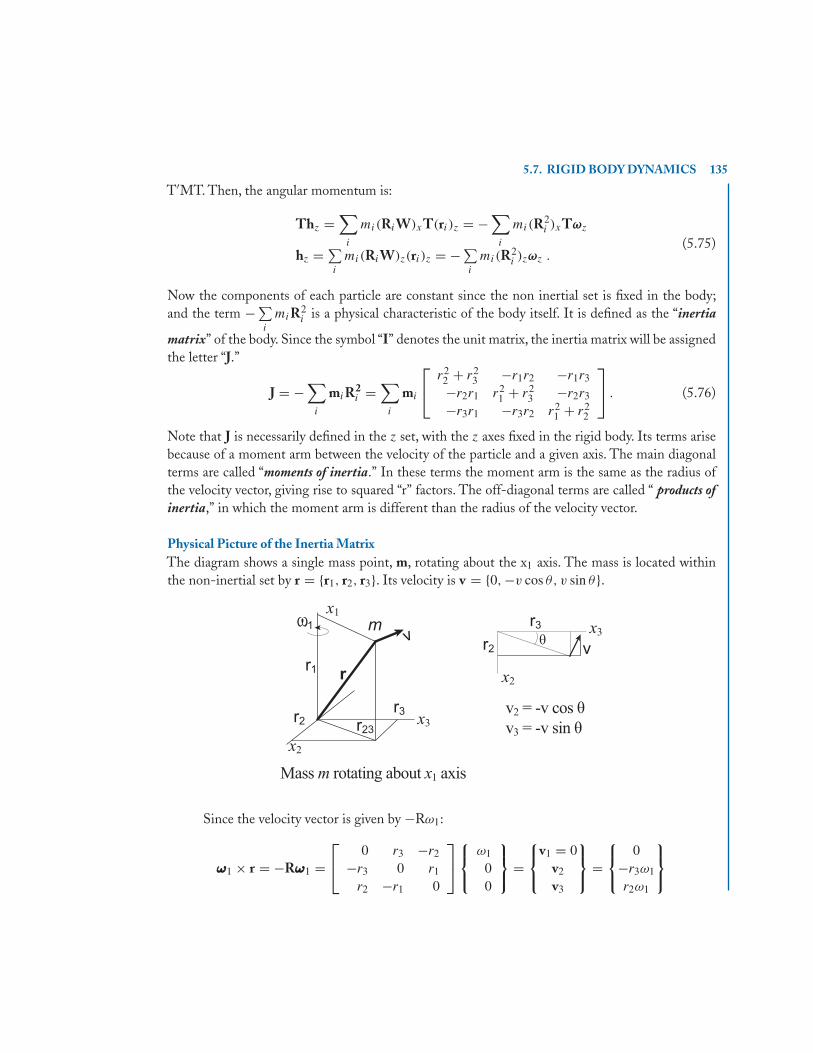
5.7. RIGID BODY DYNAMICS 135
T′MT. Then, the angular momentum is:
Thz =∑
i
mi(RiW)xT(ri )z = −∑
i
mi(R2i )xTωz
hz = ∑i
mi(RiW)z(ri )z = −∑i
mi(R2i )zωz .
(5.75)
Now the components of each particle are constant since the non inertial set is fixed in the body;and the term −∑
i
miR2i is a physical characteristic of the body itself. It is defined as the “inertia
matrix” of the body. Since the symbol “I” denotes the unit matrix, the inertia matrix will be assignedthe letter “J.”
J = −∑
i
miR2i =
∑i
mi
⎡⎣ r2
2 + r23 −r1r2 −r1r3
−r2r1 r21 + r2
3 −r2r3
−r3r1 −r3r2 r21 + r2
2
⎤⎦ . (5.76)
Note that J is necessarily defined in the z set, with the z axes fixed in the rigid body. Its terms arisebecause of a moment arm between the velocity of the particle and a given axis. The main diagonalterms are called “moments of inertia.” In these terms the moment arm is the same as the radius ofthe velocity vector, giving rise to squared “r” factors. The off-diagonal terms are called “ products ofinertia,” in which the moment arm is different than the radius of the velocity vector.
Physical Picture of the Inertia MatrixThe diagram shows a single mass point, m, rotating about the x1 axis. The mass is located withinthe non-inertial set by r = {r1, r2, r3}. Its velocity is v = {0, −v cos θ, v sin θ}.
Since the velocity vector is given by −Rω1:
ωωω1 × r = −Rωωω1 =⎡⎣ 0 r3 −r2
−r3 0 r1
r2 −r1 0
⎤⎦⎧⎨⎩
ω1
00
⎫⎬⎭ =
⎧⎨⎩
v1 = 0v2
v3
⎫⎬⎭ =
⎧⎨⎩
0−r3ω1
r2ω1
⎫⎬⎭
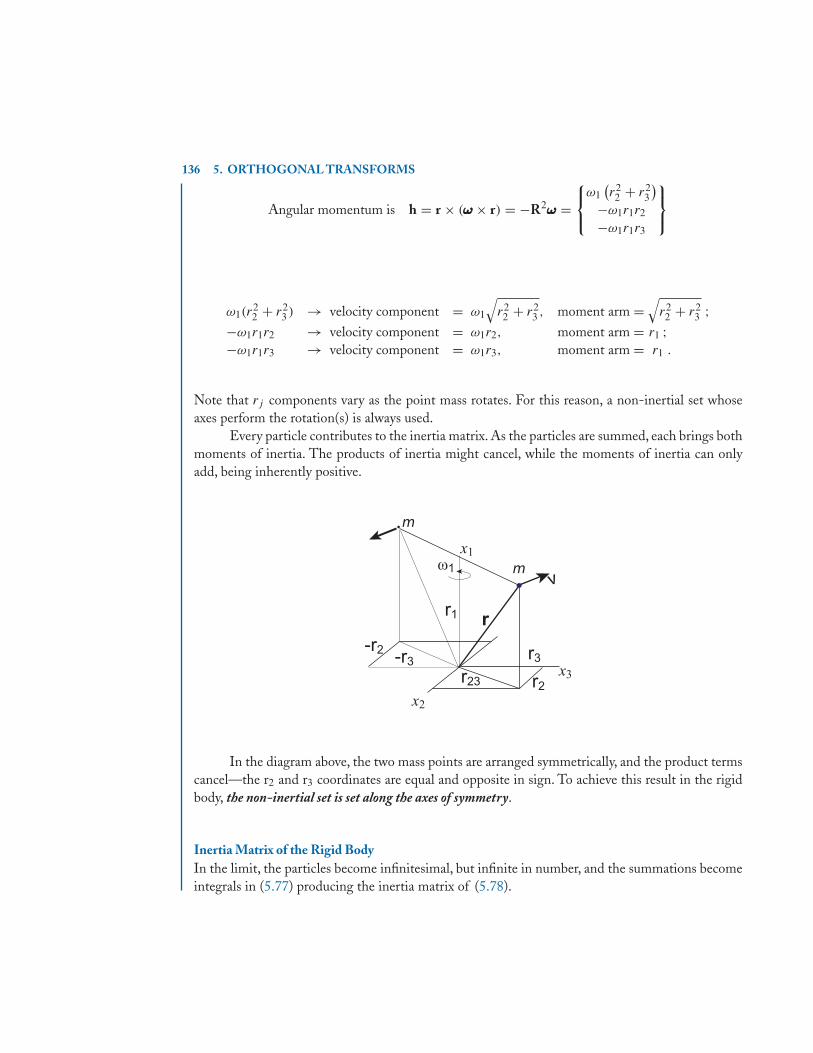
136 5. ORTHOGONAL TRANSFORMS
Angular momentum is h = r × (ωωω × r) = −R2ωωω =⎧⎨⎩
ω1(r2
2 + r23
)−ω1r1r2
−ω1r1r3
⎫⎬⎭
ω1(r22 + r2
3 ) → velocity component = ω1
√r2
2 + r23 , moment arm =
√r2
2 + r23 ;
−ω1r1r2 → velocity component = ω1r2, moment arm = r1 ;−ω1r1r3 → velocity component = ω1r3, moment arm = r1 .
Note that rj components vary as the point mass rotates. For this reason, a non-inertial set whoseaxes perform the rotation(s) is always used.
Every particle contributes to the inertia matrix. As the particles are summed, each brings bothmoments of inertia. The products of inertia might cancel, while the moments of inertia can onlyadd, being inherently positive.
m
m
In the diagram above, the two mass points are arranged symmetrically, and the product termscancel—the r2 and r3 coordinates are equal and opposite in sign. To achieve this result in the rigidbody, the non-inertial set is set along the axes of symmetry.
Inertia Matrix of the Rigid BodyIn the limit, the particles become infinitesimal, but infinite in number, and the summations becomeintegrals in (5.77) producing the inertia matrix of (5.78).
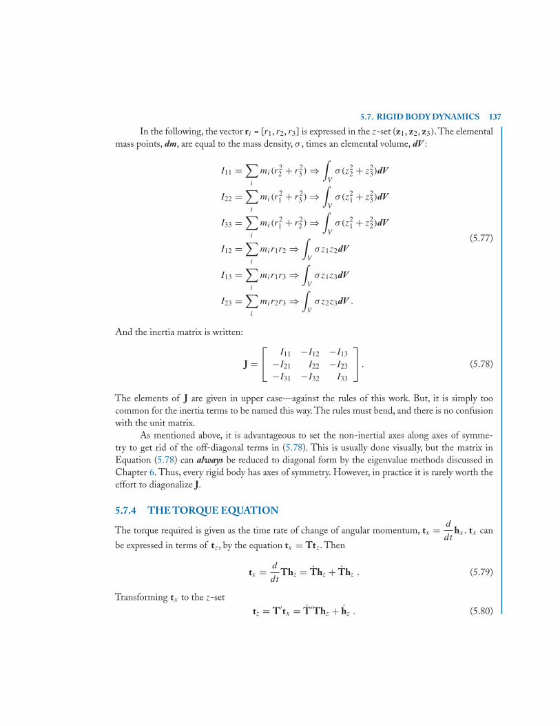
5.7. RIGID BODY DYNAMICS 137
In the following, the vector ri = {r1, r2, r3} is expressed in the z-set (z1, z2, z3). The elementalmass points, dm, are equal to the mass density, σ , times an elemental volume, dV :
I11 =∑
i
mi(r22 + r2
3 ) ⇒∫
V
σ(z22 + z2
3)dV
I22 =∑
i
mi(r21 + r2
3 ) ⇒∫
V
σ(z21 + z2
3)dV
I33 =∑
i
mi(r21 + r2
2 ) ⇒∫
V
σ(z21 + z2
2)dV
I12 =∑
i
mir1r2 ⇒∫
V
σz1z2dV
I13 =∑
i
mir1r3 ⇒∫
V
σz1z3dV
I23 =∑
i
mir2r3 ⇒∫
V
σz2z3dV .
(5.77)
And the inertia matrix is written:
J =⎡⎣ I11 −I12 −I13
−I21 I22 −I23
−I31 −I32 I33
⎤⎦ . (5.78)
The elements of J are given in upper case—against the rules of this work. But, it is simply toocommon for the inertia terms to be named this way. The rules must bend, and there is no confusionwith the unit matrix.
As mentioned above, it is advantageous to set the non-inertial axes along axes of symme-try to get rid of the off-diagonal terms in (5.78). This is usually done visually, but the matrix inEquation (5.78) can always be reduced to diagonal form by the eigenvalue methods discussed inChapter 6. Thus, every rigid body has axes of symmetry. However, in practice it is rarely worth theeffort to diagonalize J.
5.7.4 THE TORQUE EQUATION
The torque required is given as the time rate of change of angular momentum, tx = d
dthx . tx can
be expressed in terms of tz, by the equation tx = Ttz. Then
tx = d
dtThz = Thz + Thz . (5.79)
Transforming tx to the z-settz = T′tx = T′Thz + hz . (5.80)
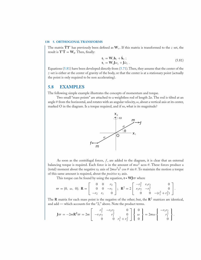
138 5. ORTHOGONAL TRANSFORMS
The matrix TT′ has previously been defined as Wx . If this matrix is transformed to the z set, theresult is T′T = Wz. Then, finally:
tz = Wzhz + hz ;tz = WzJωz + Jωz .
(5.81)
Equations (5.81) have been developed directly from (5.71). Then, they assume that the center of thez-set is either at the center of gravity of the body, or that the center is at a stationary point (actuallythe point is only required to be non accelerating).
5.8 EXAMPLESThe following simple example illustrates the concepts of momentum and torque.
Two small “mass points” are attached to a weightless rod of length 2a. The rod is tilted at anangle θ from the horizontal, and rotates with an angular velocity, ω, about a vertical axis at its center,marked O in the diagram. Is a torque required, and if so, what is its magnitude?
As soon as the centrifugal forces, f , are added to the diagram, it is clear that an externalbalancing torque is required. Each force is in the amount of mω2 acos θ . These forces produce a(total) moment about the negative x3 axis of 2mω2a2 cos θ sin θ . To maintain the motion a torqueof this same amount is required, about the positive x3 axis.
This torque can be found by using the equation, t = WJ� where
� = {0, ω, 0}; R =⎡⎣ 0 0 r2
0 0 −r1
−r2 r1 0
⎤⎦ ; R2 = 2
⎡⎣ −r2
2 r1r2 0r1r2 −r2
1 00 0 −(r2
1 + r22 )
⎤⎦ .
The R matrix for each mass point is the negative of the other; but, the R2 matrices are identical,and add — which accounts for the “2,” above. Note the product terms.
J� = −2mR2� = 2m
⎡⎣ r2
2 −r1r2 0−r1r2 r2
1 00 0 r2
1 + r22
⎤⎦⎧⎨⎩
0ω
0
⎫⎬⎭ = 2mω
⎧⎨⎩
−r1r2
r210
⎫⎬⎭ .
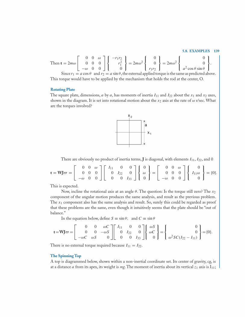
5.8. EXAMPLES 139
Then t = 2mω
⎡⎣ 0 0 ω
0 0 0−ω 0 0
⎤⎦⎧⎨⎩
−r1r2
r210
⎫⎬⎭ = 2mω2
⎧⎨⎩
00
r1r2
⎫⎬⎭ = 2mω2
⎧⎨⎩
00
a2 cos θ sin θ
⎫⎬⎭.
Since r1 = a cos θ and r2 = a sin θ , the external applied torque is the same as predicted above.This torque would have to be applied by the mechanism that holds the rod at the center, O.
Rotating PlateThe square plate, dimensions, a by a, has moments of inertia I11 and I22 about the x1 and x2 axes,shown in the diagram. It is set into rotational motion about the x2 axis at the rate of ω r/sec. Whatare the torques involved?
There are obviously no product of inertia terms, J is diagonal, with elements I11, I22, and 0
t = WJ� =⎡⎣ 0 0 ω
0 0 0−ω 0 0
⎤⎦⎡⎣ I11 0 0
0 I22 00 0 I33
⎤⎦⎧⎨⎩
0ω
0
⎫⎬⎭ =
⎡⎣ 0 0 ω
0 0 0−ω 0 0
⎤⎦⎧⎨⎩
0I11ω
0
⎫⎬⎭ = {0}.
This is expected.Now, incline the rotational axis at an angle θ . The question: Is the torque still zero? The x2
component of the angular motion produces the same analysis, and result as the previous problem.The x1 component also has the same analysis and result. So, surely this could be regarded as proofthat these problems are the same, even though it intuitively seems that the plate should be “out ofbalance.”
In the equation below, define S ≡ sin θ; and C ≡ sin θ
t =WJ� =⎡⎣ 0 0 ωC
0 0 −ωS
−ωC ωS 0
⎤⎦⎡⎣ I11 0 0
0 I22 00 0 I33
⎤⎦⎧⎨⎩
ωS
ωC
0
⎫⎬⎭=
⎧⎨⎩
00
ω2SC(I22 − I11)
⎫⎬⎭={0}.
There is no external torque required because I11 = I22.
The Spinning TopA top is diagrammed below, shown within a non-inertial coordinate set. Its center of gravity, cg, isat a distance a from its apex, its weight is mg. The moment of inertia about its vertical z1 axis is I11;
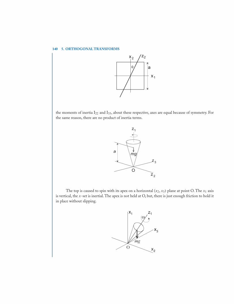
140 5. ORTHOGONAL TRANSFORMS
the moments of inertia I22 and I33, about these respective, axes are equal because of symmetry. Forthe same reason, there are no product of inertia terms.
The top is caused to spin with its apex on a horizontal (x2, x3) plane at point O. The x1 axisis vertical, the x-set is inertial. The apex is not held at O, but, there is just enough friction to hold itin place without slipping.
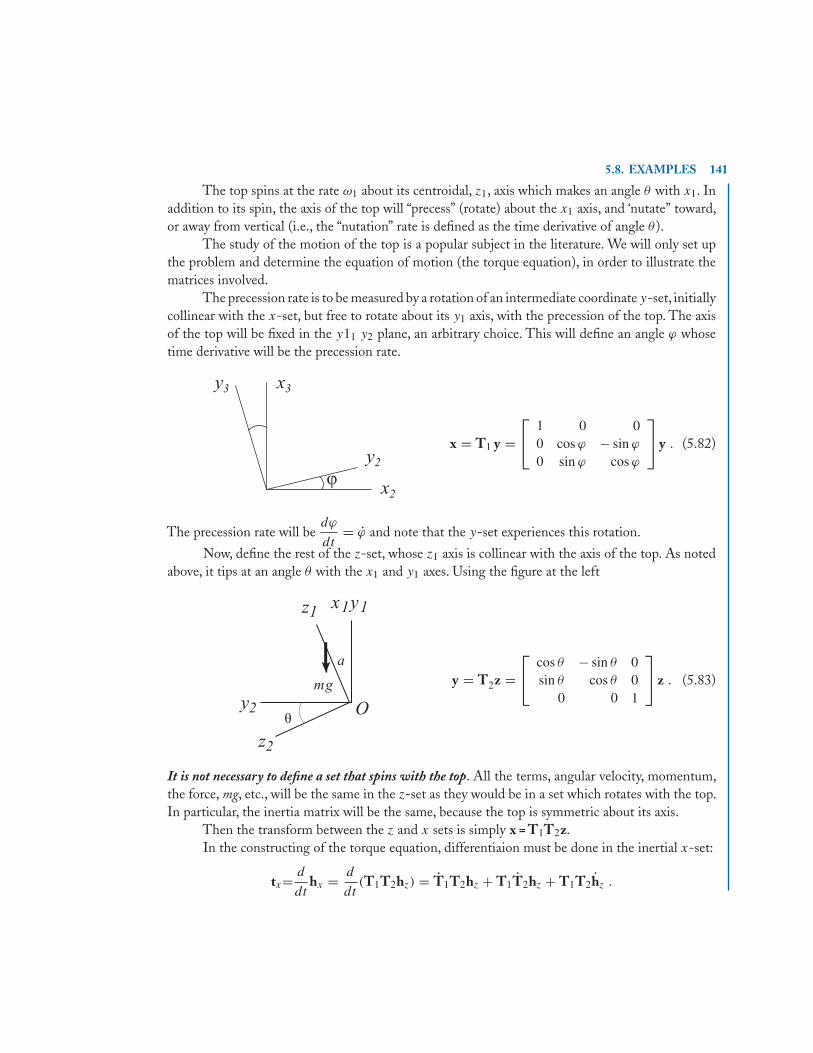
5.8. EXAMPLES 141
The top spins at the rate ω1 about its centroidal, z1, axis which makes an angle θ with x1. Inaddition to its spin, the axis of the top will “precess” (rotate) about the x1 axis, and ‘nutate” toward,or away from vertical (i.e., the “nutation” rate is defined as the time derivative of angle θ ).
The study of the motion of the top is a popular subject in the literature. We will only set upthe problem and determine the equation of motion (the torque equation), in order to illustrate thematrices involved.
The precession rate is to be measured by a rotation of an intermediate coordinate y-set, initiallycollinear with the x-set, but free to rotate about its y1 axis, with the precession of the top. The axisof the top will be fixed in the y11 y2 plane, an arbitrary choice. This will define an angle ϕ whosetime derivative will be the precession rate.
x = T1 y =⎡⎣ 1 0 0
0 cos ϕ − sin ϕ
0 sin ϕ cos ϕ
⎤⎦ y . (5.82)
The precession rate will bedϕ
dt= ϕ and note that the y-set experiences this rotation.
Now, define the rest of the z-set, whose z1 axis is collinear with the axis of the top. As notedabove, it tips at an angle θ with the x1 and y1 axes. Using the figure at the left
y = T2z =⎡⎣ cos θ − sin θ 0
sin θ cos θ 00 0 1
⎤⎦ z . (5.83)
It is not necessary to define a set that spins with the top. All the terms, angular velocity, momentum,the force, mg, etc., will be the same in the z-set as they would be in a set which rotates with the top.In particular, the inertia matrix will be the same, because the top is symmetric about its axis.
Then the transform between the z and x sets is simply x = T1T2z.In the constructing of the torque equation, differentiaion must be done in the inertial x-set:
tx= d
dthx = d
dt(T1T2hz) = T1T2hz + T1T2hz + T1T2hz .
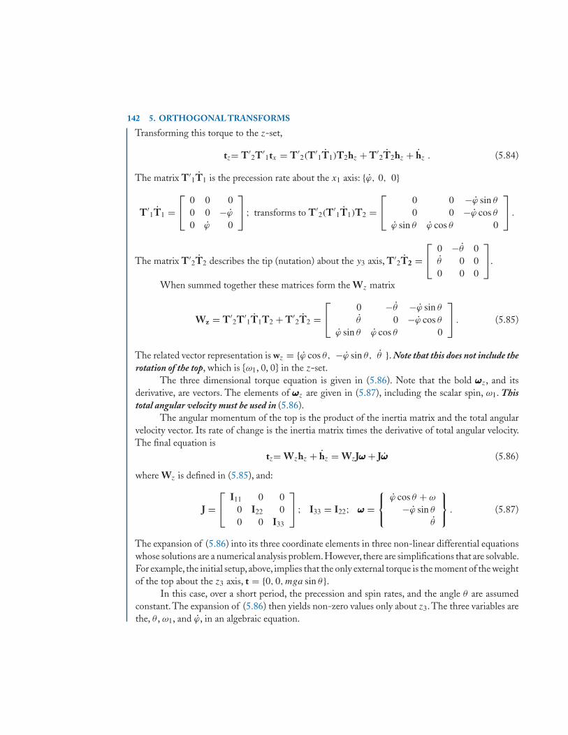
142 5. ORTHOGONAL TRANSFORMS
Transforming this torque to the z-set,
tz= T′2T′
1tx = T′2(T′
1T1)T2hz + T′2T2hz + hz . (5.84)
The matrix T′1T1 is the precession rate about the x1 axis: {ϕ, 0, 0}
T′1T1 =
⎡⎣ 0 0 0
0 0 −ϕ
0 ϕ 0
⎤⎦ ; transforms to T′
2(T′1T1)T2 =
⎡⎣ 0 0 −ϕ sin θ
0 0 −ϕ cos θ
ϕ sin θ ϕ cos θ 0
⎤⎦ .
The matrix T′2T2 describes the tip (nutation) about the y3 axis, T′
2T2 =⎡⎣ 0 −θ 0
θ 0 00 0 0
⎤⎦.
When summed together these matrices form the Wz matrix
Wz = T′2T′
1T1T2 + T′2T2 =
⎡⎣ 0 −θ −ϕ sin θ
θ 0 −ϕ cos θ
ϕ sin θ ϕ cos θ 0
⎤⎦ . (5.85)
The related vector representation is wz = {ϕ cos θ, −ϕ sin θ, θ }. Note that this does not include therotation of the top, which is {ω1, 0, 0} in the z-set.
The three dimensional torque equation is given in (5.86). Note that the bold ωωωz, and itsderivative, are vectors. The elements of ωωωz are given in (5.87), including the scalar spin, ω1. Thistotal angular velocity must be used in (5.86).
The angular momentum of the top is the product of the inertia matrix and the total angularvelocity vector. Its rate of change is the inertia matrix times the derivative of total angular velocity.The final equation is
tz= Wzhz + hz = WzJωωω + Jωωω (5.86)
where Wz is defined in (5.85), and:
J =⎡⎣ I11 0 0
0 I22 00 0 I33
⎤⎦ ; I33 = I22; ωωω =
⎧⎨⎩
ϕ cos θ + ω
−ϕ sin θ
θ
⎫⎬⎭ . (5.87)
The expansion of (5.86) into its three coordinate elements in three non-linear differential equationswhose solutions are a numerical analysis problem.However, there are simplifications that are solvable.For example, the initial setup, above, implies that the only external torque is the moment of the weightof the top about the z3 axis, t = {0, 0, mga sin θ}.
In this case, over a short period, the precession and spin rates, and the angle θ are assumedconstant. The expansion of (5.86) then yields non-zero values only about z3. The three variables arethe, θ , ω1, and ϕ, in an algebraic equation.
5.9. EXERCISES 143
5.9 EXERCISES
5.1. An Airplane is to fly,direct, from a point A,74 degrees west longitude and 41 degrees (north)latitude (roughly on the east coast of the US), to a point B, 122 degrees west longitude and41 degrees latitude (roughly on the west coast). Assume a spherical earth, with a radiusequal to 4000mi.
(a) Construct a coordinate y-set at the point A, as in Equation (5.8) of the text.
(b) What is the great circle distance between the two points?
(c) If the airplane simply flies west, along the 41 degree latitude, what is that distance?
(d) After takeoff, what is the correct heading to fly the great circle path?
5.2. A two-dimensional transform matrix is T =⎡⎣ cos
π
5sin
π
5− sin
π
5cos
π
5
⎤⎦. Find T10.
5.3. Given;
R =⎡⎣ 0 −r3 r2
r3 0 −r1
−r2 r1 0
⎤⎦ ; W =
⎡⎣ 0 −ω3 ω2
ω3 0 −ω1
−ω2 ω1 0
⎤⎦ ; r =
⎧⎨⎩
r1
r2
r3
⎫⎬⎭ ; � =
⎧⎨⎩
ω1
ω2
ω3
⎫⎬⎭ .
(a) Is RWr equal to r×(ω×r) or equal to (r×ω)×r ?
(b) Is RWr = R2ω ?
(c) Is W2r equal to ω × (ω×r) or equal to (ω × ω)×r ?
5.4. It has been shown that no external torques are required to maintain the
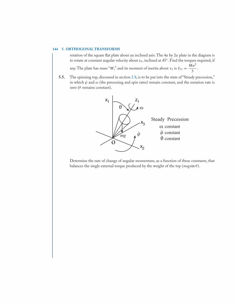
144 5. ORTHOGONAL TRANSFORMS
rotation of the square flat plate about an inclined axis. The 4a by 2a plate in the diagram isto rotate at constant angular velocity about z1, inclined at 45◦. Find the torques required, if
any. The plate has mass “M ,” and its moment of inertia about x1 is I11 = Ma2
3.
5.5. The spinning top, discussed in section 5.8, is to be put into the state of “Steady precession,”in which ϕ and ω (the precessing and spin rates) remain constant, and the nutation rate iszero (θ remains constant).
Determine the rate of change of angular momentum, as a function of these constants, thatbalances the single external torque produced by the weight of the top (magsin θ ).
145
C H A P T E R 6
Matrix Eigenvalue Analysis
6.1 INTRODUCTIONMatrix analysis is particularly interesting because of the insight that it brings to so many areas ofengineering. With the advent of the modern computer, much of the numerical labor is at leasttransferred into the fascinating realm of programming.
Perhaps the single most interesting matrix analysis is that which will now be discussed. It hasfundamental bearing on the solution to many differential equations governing vibration problems,and the analysis of electrical networks. The eigenvalue problem is basically concerned with thetransformation of vectors and matrices in a most advantageous fashion.
6.2 THE EIGENVALUE PROBLEMThe beginning is simple enough: Concerning the transform
Ax = y (6.1)
where A is a general, real, square matrix, we ask whether or not an (input) x vector can be foundsuch that the (output) y vector is proportional to x. That is:
Ax = λx . (6.2)
The constant λ is the (scalar) factor of proportionality. We can bring λx to the left side of (6.2):
[A − λI]x = A(λ)x = 0 . (6.3)
In (6.3), the notation [A – λI] is used rather than the more familiar (A – λI) in order to emphasizethat the quantity within the “[. .]” is a square matrix. A is nXn, x is nX1, I is the nXn unit matrix;so the right side zero is an nX1 null column. The matrix [A - λI] is often referred to as A(λ), the“Lambda Matrix,” or “Characteristic Matrix.”
When A is not symmetric, the “companion” Equation (6.4) must also be considered:
z[A − λI] = 0 (6.4)
where, now, z is 1Xn (a row vector), and the 0 is a null 1Xn row. As will be seen, these two equationsare “bound together,” and will be solved together.
From Chapter 4, the homogeneous sets (6.3) and (6.4) have nontrivial solution iff the matrix[A – λI] is singular. Furthermore, in this treatment of the problem, we will require that the rank ofthe matrix [A – λI] be n-1. This condition is met by most engineering problems of interest.
146 6. MATRIX EIGENVALUE ANALYSIS
6.2.1 THE CHARACTERISTIC EQUATION AND EIGENVALUESIn order for [A - λI] to be singular, the determinant must vanish:
∣∣A − λI∣∣ = (−1)n
∣∣∣∣∣∣∣∣a11 − λ a12 · · · a1n
a21 a22 − λ · · · · · ·· · · · · · a22 − λ · · ·an1 an2 · · · ann − λ
∣∣∣∣∣∣∣∣= 0. (6.5)
The expansion of the determinant in (6.5) clearly will result in a polynomial of degree n. Themultiplier (-1)n is used simply to cause the coefficient of λn to be positive (and, the determinant (6.5)would be more accurately written as |λI−A|). Thus,
f (λ) = λn + c1λn−1 + . . . cn−1λ + cn = 0 . (6.6)
f (λ) is called the “characteristic equation” and the polynomial is called the “characteristic polyno-mial” related to the matrix A. The coefficients, ck , are all functions of the [aij ] elements, and thecoefficient cn is equal to the determinant of A (and the product of the λ values). Now, represent thepolynomial in (6.6) in its factored form:
f (λ) = (λ − λ1)(λ − λ2)(λ − λ3) · · · (λ − λn) = 0 (6.7)
and it is clear that for each λ = λj ,f (λj ) = 0.These roots of the characteristic equation are called the“eigenvalues,” or “characteristic values” of A. Since (6.6) and (6.5) represent the same equation,these λj values also cause the determinant in (6.5) to vanish. If the λj eigenvalues are all distinct (i.e.,no two roots the same), then the above constraint that the rank of the determinant be n − 1 will bemet. Except for a short discussion concerning what happens when multiple roots occur, this chapterwill assume distinct roots. In the general case, in which A is not symmetric, the eigenvalues maybe complex numbers. While this fact is not much of a conceptual difficulty, it does pose calculationproblems.
Now, consider the case λ = λ1. The determinant |A(λ1)| is zero and there will be exactly onesolution to each of the Equations (6.3) and (6.4) above. These solutions, being associated with theeigenvalue, λ1, are known as “eigenvectors,” or “characteristic vectors.” Equation (6.3) will yield acolumn vector, and (6.4) will yield a row vector. These vectors will “emerge” together.
The adjoint of [A – λ1I] will be of unit rank. All its rows (columns) will be proportional toeach other (some, but not all, of the rows (columns) of the adjoint may be null). Denote the roweigenvector as u1, and the column eigenvector as v1. The adjoint of [A – λ1I] can be written
Aa(λ1) = [A − λ1I]adj = k{v1}[u1] . (6.8)
The vector product given in (6.8) is nX1X1Xn = nXn. It is certainly not the dot product of u1 andv1. (In fact, every matrix of unit rank can be written as this type of single column times single row.That is essentially the definition of rank = 1.)
6.2. THE EIGENVALUE PROBLEM 147
Any column of the adjoint of (6.8) solves [A – λ1I]x = 0. Yet, there can be only one solution.Thus, all the adjoint columns must be the same—i.e., proportional, differing only in magnitude.That is, only the eigenvector’s direction is obtained .
Similarly, every (non-zero) row of the adjoint solves z[A – λ1I] = 0 (note, again that thisis a row equation). Then, for any given eigenvalue, (6.8) yields exactly one row, and one columneigenvector. And, since the vector magnitudes are arbitrary, we can always choose scaling such thatthe dot product of u1 and v1 is equal to +1 (unity).
In the same way, all n eigenvectors are obtained from their respective adjoint matrices. And,each time they are scaled to +1. It will now be shown that vj is orthogonal to ui , for the subscript i
not equal to j . Write (v for column vectors, and u for rows)
Avj = λj vj ; Note that vj is (nX1)uiA = λiui ; Note that ui is (1Xn) .
(6.9)
Premultiply the first of (6.9) by [ui] and postmultiply the second by {vj }. The left sides of bothequations will then be identical. If the two are subtracted, the result is
ui • vj (λi − λj ) = 0 . (6.10)
Since the eigenvalues are distinct (by hypothesis), then (λi – λj ) cannot be zero. Thus, the dotproduct ui•vj must be zero, proving that the two eigenvectors are orthogonal. But, the originalchoice of i and j was arbitrary. So, the assertion of orthogonality must be true for any choice. Then,if all the row eigenvectors are collected into the square matrix, U, and the column eigenvectorscollected into V (and remembering that ui•vi can be normalized to +1):
UV = VU = I, (the unit matrix) . (6.11)
Also, the entire eigenvalue problem can be displayed in the following 2 equations:
AV = V�
UA = �U. (6.12)
In (6.12), the matrix, �, is a diagonal matrix whose main diagonal elements are the eigenvalues –arranged, carefully, in the same order in which the eigenvectors are placed in the matrices U and V.Now, choose the first of the Equations (6.12), and premultiply by U. Using (6.11), the result is:
UAV = � . (6.13)
That is, the A matrix is transformed by U and V into its “eigenvalue matrix,” �.
6.2.2 SYNTHESIS OF A BY ITS EIGENVALUES AND EIGENVECTORSPremultiplying the second of Equations (6.12) by V reveals an interesting, and useful result.
A = V�U .
148 6. MATRIX EIGENVALUE ANALYSIS
The eigenvalue analysis “resolves” matrix A into its component eigenvalues and vectors.This becomesmore evident if it is remembered that premultiplying U by � has the effect of multiplying everyelement of row uj by its corresponding λj . Now, simply visualize this and also partition V by columnsand the �U product by rows:
A =n∑j
λj {vj }[uj ] . (6.14)
A is shown as a sum of n matrices; λj {vj }[uj ], each nXn, and each composed only of correspondingeigenvalues and eigenvectors. It is instructive to postmultiply the eigenvector vk on both sidesof (6.14)
Avk =n∑j
λj {vj }[uj ]{vk} .
Now, all the products uj•vk vanish (the eigenvectors are orthogonal), except the uk•vk one (whichis normalized to +1). Then
Avk = λkvk
which is the same as Equation (6.2), with the appropriate subscripts.In (6.14), if any one of the nXn matrices in the summation were to be subtracted away, a new
matrix, say B, would result. B would have all the same eigenvalues and vectors that A possesses –except the one subtracted away. This fact is useful in “matrix iteration” (not yet discussed here), inwhich iterative techniques are used to obtain eigenvalues and vectors, one at a time. When one set isfound, its effects can be subtracted away, to move on to iterate for the next. See the article on matrixiteration in Section 6.7.2 of this chapter.
6.2.3 EXAMPLE ANALYSIS OF A NONSYMMETRIC 3X3To illustrate the eigenvalue problem numerically, consider the following 3X3:
A =⎡⎣ 25 −44 18
12 −21 8−3 6 −4
⎤⎦ .
This matrix is a particularly simple one numerically. But, its analysis will nevertheless illustrate theeigenvalue problem. Eigenvalues will be denoted using λ, and the characteristic equation is theexpansion of the determinant:
f (λ) = (−1)3
∣∣∣∣∣∣25 − λ −44 18
12 −21 − λ 8−3 6 −4 − λ
∣∣∣∣∣∣ = 0 . (6.15)
Since (−1)3 = −1, negate the first row:
|(λ − 25) + 44 − 18| ,
6.2. THE EIGENVALUE PROBLEM 149
and expand by first minors of the first row,
f (λ) = (λ − 25)[(−21 − λ)(−4 − λ) − 48] − 44[12(−4 − λ) + 24]− 18[72 + 3(−21 − λ)] = 0
which reduces algebraically to:f (λ) = λ3 − 7λ − 6 = 0 . (6.16)
Notice that in this case there is no λ2 term (i.e., its coefficient is zero), and that the “trace” of A(the sum of its diagonal elements) is also zero. In fact, the (negative) trace of A is always equal toits coefficient in its characteristic polynomial.
By inspection, −1 is a root of (6.16). Dividing by (λ + 1), and factoring the quadratic:
f (λ) = (λ + 1)(λ2 − λ − 6) = (λ + 1)(λ + 2)(λ − 3) . (6.17)
The three roots, −1, −2, and 3, are the three eigenvalues of A. For each eigenvalue there will betwo eigenvectors—a row eigenvector, and a column eigenvector.
With λ1 = −1, and denoting [A – λ1I], as A(λ1):
A(λ1) =⎡⎣ 26 −44 18
12 −20 8−3 6 −3
⎤⎦ ;
26x1 − 44x2 + 18x3 = 012x1 − 20x2 + 8x3 = 0−3x1 + 6x2 − 3x3 = 0
.
The solution of the linear equation set at the above/right determines the eigenvector, v1. Since A(λ1)
is known to be singular, this set must have a non-trivial solution. One way to do this is to set x3
arbitrarily (say, x3 = 1), delete the third equation, and solve the remaining two variables:
26x1 − 44x2 = −1812x1 − 20x2 = −8
From which it is found that x1 = x2 = x3 = 1.|A(λ1)| is equal to zero. However, the adjoint matrix must have at least one non zero row and
column (the rank of A(λ1) is n − 1). Then, by calculating the adjoint, both row and columns arefound:
A(λ1) =⎡⎣ 26 −44 18
12 −20 8−3 6 −3
⎤⎦ ; Aa(λ1) =
⎡⎣ 12 −24 8
12 −24 812 −24 8
⎤⎦ . (6.18)
From this adjoint, any row can be chosen as the row vector, and any column can be chosen asthe column vector, for example [12, −24, 8] for the row vector, and {12, 12, 12} for the column.However, the eigenvectors emerge in direction only, then any multiples of these vectors are alsoeigenvectors. Then:
u1 = [3, −6, 2] and v1 = {1, 1, 1}
150 6. MATRIX EIGENVALUE ANALYSIS
where u1 denotes the row vector, and v1 denotes the column. Since u1 • v1 product must be 1,normalize by multiplying u1 by −1.
u1 = [−3, 6, −2] and v1 = {1, 1, 1}Now, if these two vectors are truly eigenvectors they must solve
(A − λ1I)v1 = 0; & u1(A − λ1I) = 0 .
And they do: [ −3 6 −2]⎡⎣ 26 −44 18
12 −20 8−3 6 −3
⎤⎦ = [
0 0 0]
and
⎡⎣ 26 −44 18
12 −20 8−3 6 −3
⎤⎦⎧⎨⎩
111
⎫⎬⎭ =
⎧⎨⎩
000
⎫⎬⎭ .
With λ2 = −2
A(λ2) =⎡⎣ 27 −44 18
12 −19 8−3 6 −2
⎤⎦ ; Aa(λ2) =
⎡⎣ 10 20 −10
0 0 015 −30 15
⎤⎦ . (6.19)
In the same manner as before,
u2 = [−1, 2, −1] and v2 = {2, 0, −3}Note that the adjoint has a zero row, which must not be chosen as an eigenvector. This is
simple by sight, but if the computer is choosing eigenvectors, it must be taught to avoid such things.With λ3 = 3:
A(λ3) =⎡⎣ 22 −44 18
12 −24 8−3 6 −7
⎤⎦ ; Aa(λ3) =
⎡⎣ 120 −200 80
60 −100 400 0 0
⎤⎦ . (6.20)
u3 = [3, −5, 2] and v3 = {2, 1, 0}Now that the eigenvectors have all been chosen, and normalized uk • vk = 1, the 3X3 U and Vmatrices are:
U =⎡⎣ −3 6 −2
−1 2 −13 −5 2
⎤⎦ ; and V =
⎡⎣ 1 2 2
1 0 11 −3 0
⎤⎦ . (6.21)
These matrices are inverses, i.e., UV = VU = I, and
AV = V� (See Equations (6.12))
6.2. THE EIGENVALUE PROBLEM 151
where � is the (3X3) diagonal eigenvalue matrix. Now, postmultiply by U:
AVU = A = V�U . (6.22)
Which shows the synthesis of A by its eigenvalues and eigenvectors. In this example:
V�U =⎡⎣ 1 2 2
1 0 11 −3 0
⎤⎦⎡⎣ −1 0 0
0 −2 00 0 3
⎤⎦⎡⎣ −3 6 −2
−1 2 −13 −5 2
⎤⎦ =
⎡⎣ 25 −44 18
12 −21 8−3 6 −4
⎤⎦ = A .
An important result. Alternatively, the matrices U and V “diagonalize” the original matrix:
UAV = � (6.23)
UAV =⎡⎣ −3 6 −2
−1 2 −13 −5 2
⎤⎦⎡⎣ 25 −44 18
12 −21 8−3 6 −4
⎤⎦⎡⎣ 1 2 2
1 0 11 −3 0
⎤⎦ =
⎡⎣ −1 0 0
0 −2 00 0 3
⎤⎦ .
Now, to illustrate the point about the synthesis of A via its eigenvalues and vectors, from the matrixA, subtract the 3X3 = λ1{v1}[u1]:
B =⎡⎣ 25 −44 18
12 −21 8−3 6 −4
⎤⎦−
⎡⎣ −3 6 −2
−3 6 −2−3 6 −2
⎤⎦ =
⎡⎣ 22 −38 16
9 −15 6−6 12 −6
⎤⎦ . (6.24)
An analysis of B shows that it still possesses the eigenvalues −2, and 3, but, in place of λ1 = −1, itsλ1 is zero (B is singular). Interestingly, all its eigenvectors are the same—even u1 and v1. However,u1 and v1 can play no part in the synthesis of B, because these are multiplied by zero.
6.2.4 EIGENVALUE ANALYSIS OF SYMMETRIC MATRICESIn the general (non-symmetric) case, 2 equations are required to define the eigenvalue problem(Equations (6.3) and (6.4)). When the given matrix is symmetric, a simplification occurs. If (6.3) istransposed (λI is diagonal) the result is x′[A′ – λ I] = 0. But, in this case A′ = A, and the result isthat the row vector is simply the transposed column vector.
For any eigenvalue, λi the adjoint matrix [A – λiI]adj is also a symmetric matrix, proportionalto the product of viv ′
i . Any nonzero row or column can be chosen.The orthogonality of these eigenvectors is shown in the following way. For any two vectors,
write:Avi = λivi
Avj = λj vj .(6.25)
Now, premultiply the first of these by vj and the second by vi .
v ′j Avi = λiv ′
j vi
v ′iAvj = λj v ′
ivj .(6.26)
152 6. MATRIX EIGENVALUE ANALYSIS
If the second of these is transposed, the left sides become identical, because A is symmetric. Then,when the two are subtracted, as before, the eigenvectors must be orthogonal (again assuming distincteigenvalues). This orthogonality can be expressed in terms of all the eigenvectors, as
V′V = I (compare with (6.11)) . (6.27)
And the entire eigenvalue problem can be displayed in the single equation,
AV = V� (compare with (6.12)) . (6.28)
The diagonalization of A is shown by premultiplying by V′
V′AV = V′V� = � (compare with (6.13)) . (6.29)
The synthesis of A is given by postmultiplying: AV V′ = A = V�V′ and (6.14) becomes:
A =n∑j
λj {vj }[vj ] . (6.30)
Again note that the vector product shown here is nX1X1Xn, resulting in nXn matrices.
6.3 GEOMETRY OF THE EIGENVALUE PROBLEMThe dot product of a vector x, times itself, is equal to the sum of squares of its elements. If this sumis equated to unity, we have
x′x = x21 + x2
2 + · · · + x2n = 1 .
In two or three dimensions, the above equation is identified as that of a circle, or sphere, of unitradius. By analogy, the n dimensional case, written above, is called an n-dimensional sphere.
The dot product of x into the vector �x, where � is a diagonal matrix, is x′�x. Equated tounity:
x′�x = λ1x21 + λ2x
22 + · · · + λnx
2n = 1 . (6.31)
Depending upon the sign of the λ values, the above equation in three dimensions would be an ellipsoidor hyperboloid. For our purposes, it is most beneficial to visualize an ellipsoid. In the accompanyingfigure,note that the coordinate axes are aligned along the principal axes of the ellipsoid.But, in (6.31),if we affect an arbitrary orthogonal coordinate transform, x = Tq. Then:
q′T′�Tq = q′Aq = 1 (6.32)
and note that A is a symmetric (not diagonal) matrix whose eigenvalues are in � and whose eigen-vectors are in the transform matrix T.
Chapter 5, shows that such a transform amounts to a series of rotations about the axes of arectangular coordinate system—apparently, in this case, rotating the axes away from the principal axes
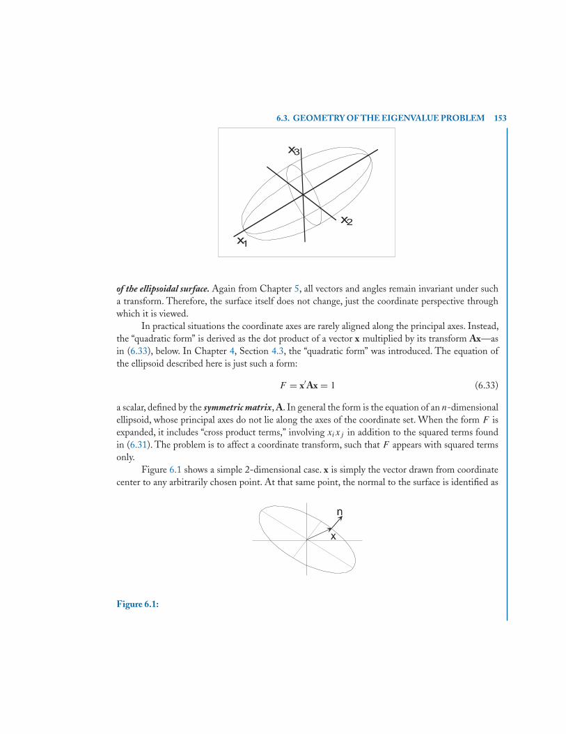
6.3. GEOMETRY OF THE EIGENVALUE PROBLEM 153
of the ellipsoidal surface. Again from Chapter 5, all vectors and angles remain invariant under sucha transform. Therefore, the surface itself does not change, just the coordinate perspective throughwhich it is viewed.
In practical situations the coordinate axes are rarely aligned along the principal axes. Instead,the “quadratic form” is derived as the dot product of a vector x multiplied by its transform Ax—asin (6.33), below. In Chapter 4, Section 4.3, the “quadratic form” was introduced. The equation ofthe ellipsoid described here is just such a form:
F = x′Ax = 1 (6.33)
a scalar, defined by the symmetric matrix, A. In general the form is the equation of an n-dimensionalellipsoid, whose principal axes do not lie along the axes of the coordinate set. When the form F isexpanded, it includes “cross product terms,” involving xixj in addition to the squared terms foundin (6.31). The problem is to affect a coordinate transform, such that F appears with squared termsonly.
Figure 6.1 shows a simple 2-dimensional case. x is simply the vector drawn from coordinatecenter to any arbitrarily chosen point. At that same point, the normal to the surface is identified as
Figure 6.1:
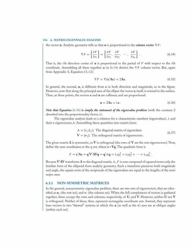
154 6. MATRIX EIGENVALUE ANALYSIS
the vector n. Analytic geometry tells us that n is proportional to the column vector ∇F :
∇F ={
∂F
∂xi
}={
∂F
∂x1,
∂F
∂x2, · · · ,
∂F
∂xn
}. (6.34)
That is, the ith direction cosine of n is proportional to the partial of F with respect to the ithcoordinate. Assembling all these together as in (6.34) derives the ∇F column vector. But, againfrom Appendix A, Equation (A.12):
∇F = ∇(x′Ax) = 2Ax . (6.35)
In general, the normal, n, is different from x in both direction and magnitude, as in the figure.However, note that along the principal axes of the ellipse the vector x, itself, is normal to the surface.Then, at these points, the vectors x and n are collinear, and are proportional:
n = 2Ax = λx . (6.36)
Note that Equation (6.36) is simply the statement of the eigenvalue problem (with the constant 2absorbed into the proportionality factor, λ).
The eigenvalue analysis leads to a solution for n characteristic numbers (eigenvalues), λ andtheir n eigenvectors, v. Assembling these quantities into matrix form:
� = [λj δij ]; The diagonal matrix of eigenvalues
V = [vj ]; The orthogonal matrix of eigenvectors .(6.37)
The given matrix A is symmetric, so V is orthogonal (the rows of V are the row eigenvectors). Now,define the new coordinates as the q-set, where x = Vq. The quadratic form is
F = x′Ax = q′V ′AVq = q′�q = λ1q21 + λ2q
22 + · · · + λnq
2n .
Because V′AV transforms A to the diagonal matrix,�,F is now composed of squared terms only, thefamiliar form of the ellipsoid from analytic geometry. Such a transform preserves both magnitudeand angle, the square roots of the reciprocals of the eigenvalues are equal to the lengths of the semimajor axes.
6.3.1 NON-SYMMETRIC MATRICESIn the general, nonsymmetric eigenvalue problem, there are two sets of eigenvectors, that are iden-tified as ui (the row set), and vi (the column set). When the full complement of vectors is gatheredtogether, these occupy the rows and columns, respectively, of U, and V. However, neither U nor Vis orthogonal. Neither of these, then, represent rectangular coordinate sets. Instead, they representbase vectors in two “skewed” systems in which the u (as well as the v) axes are at oblique angles(within each set).
6.3. GEOMETRY OF THE EIGENVALUE PROBLEM 155
But, U and V are inverses. Then, ui•vj = δij . That is, the u axes are orthogonal to the v. Inthe oblique (nonsymmetric) case, it takes two sets of coordinates to take part in a coordinate transformand, the diagonalization of a quadratic form (now called a “bilinear form”).
In the rectangular set, a given vector, r = {r1, r2, · · ·, rn}, is represented by the rj set of numbers,each of which is determined by taking the dot product of r with the j th base vector. A transformof r to a new orthogonal set is given by Vr, where V is an orthogonal transform matrix relating thenew unit vector axes to the old ones.
But, in an oblique system, this convenience is absent. Any vector, say r, has two sets ofcoordinate values:
r ={
r1v1 r2v2 · · · rnvn
ρ1u1 ρ2u2 · · · ρnun
}
where ui and vi represent unit vectors. That is (for example), the scalar r1 is the coordinate of r inthe direction of the unit vector v1, while ρ1 is the coordinate of r in the direction of the unit vectoru1. Furthermore, in order to determine r1 we must take the dot product of r, not with the unit vectorv1, but, with the unit vector, u1. Similarly, given another vector y:
y ={
y1, · · · , yn in the v-setψ1, · · · , ψn in the u-set
}
(the unit vectors are omitted) the dot product of the two vectors is given by
r • y = r1ψ1 + r2ψ2 + · · · + rnψn = ρ1y1 + ρ2y2 + · · · + ρnyn .
Dot products must be taken between coordinates of the two sets. The products involving terms like riyi ,or ρiψi , have absolutely no meaning. With this in mind, we write the form:
ξ ′Ax = 1 (A nonsymmetric) .
The principal axes of the form are still those that are normal to the surface, and the form is once againexpressed in the defining equation Ax = λx. However, ξ and x are the two different representationsof the same entity. Another expression is required in order to derive “the other half ” of the normalto the surface. That is, the transposed set
(ξ ′Ax)′ = x′A′ξ = 1 .
This time the defining equation is A′ξ = λξ which will bring out the companion set coordinates ofthe vector which is proportional to the normal. Note here, that ξ is represented as a column. In ourdevelopment of the eigenvalue problem, this same equation is written as a row equation because itwas important to identify this half of the problem, “the row half.” That is:
A′ξ = λ ξ ⇔ ξ A = λ ξ
are the same equation, but the second form, with ξA makes it clear that ξ is a row vector.
156 6. MATRIX EIGENVALUE ANALYSIS
The eigenvalue analysis finds that two sets of n vectors emerge (as in Section 6.2), and theyare mutually orthogonal. In the geometric sense, there is only one set of principal axes, and theseare orthogonal. But the analysis of them is required to take place within the two oblique, mutuallyorthogonal systems.
Once this is accomplished, a transform is made to the principal axes, which are an orthogonalset. The extra complication is removed. Thus, with the transforms ξ =z′U and x = Vz.
F = ξAx = z′UAVz = z′�z = 1 .
And the transformation of F is complete.Yet, not all the complications can be avoided. In the symmetric case, the eigenvalues are always
real , and a full complement of eigenvectors can always be determined . In the general case this is nottrue. Both eigenvalues and eigenvectors may be complex numbers; the matrices U, V, and �, thencomplex. When eigenvalues are repeated in the symmetric case, it simply means that ellipses becomecircles, providing another degree of choice in choosing rectangular axes.
In the oblique case, when repeated eigenvalues occur, it might be that some of the obliqueaxes collapse into one, and it cannot be guaranteed that a full set of eigenvectors can be found. Thus,the eigenvalue problem and its geometric representation is far easier when the quadratic form isoriginally given in terms of a symmetric matrix A.
Matrices that arise in engineering problems are often symmetric, and the associated quadraticform has physical as well as geometric significance. For this reason the symmetric eigenvalue problemis particularly important. However, it is also true that eigenvalue analysis is often required of non-symmetric matrices, with complex roots and vectors. For example, the kinetic and potential energiesin vibrating systems are described by quadratic forms. However, when energy dissipation terms areinvolved, the system is dynamically described by a nonsymmetric matrix, with complex eigenvaluesand eigenvectors. Such systems will be discussed in the following chapter.
6.3.2 MATRIX WITH A DOUBLE ROOTWhen a non symmetric matrix, A, is found to have a repeated root, there is the question of whetheror not the matrix is defective—does A possess a full complement of eigenvectors?
As an example consider A =⎡⎣ 0 −2 −2
1 3 10 0 2
⎤⎦
whose characteristic polynomial is (λ − 1)(λ − 2)(λ − 2).For the eigenvalue λ = 1 the adjoint of A(λ1) is the product [A – 2I][A – 2I], from which a
row and a column vector emerge. For the double root, λ = 2, the matrix [A − I] [A − 2I] is null (no
6.4. THE EIGENVECTORS AND ORTHOGONALITY 157
row or column can be chosen as an eigenvector). So, look at [A − 2I]x
[A − 2I]x = A(λ2)x =⎡⎣ 2 2 2
−1 −1 −10 0 0
⎤⎦ x .
This matrix clearly has rank = 1. Two independent vectors can be found that are orthogonal to therows/columns of A(λ2).Thus, A is not defective—it has all three eigenvectors. If A(λ2) had rank = 2,only one eigenvector could be found, and A would be defective. This A matrix satisfies an equationf (A) that is of lower rank than the Cayley-Hamilton equation, namely [A − 2I] [A − 2I] = 0.Thisleaves just enough room for the definition of the necessary eigenvectors.
Now, consider the matrix below. Its characteristic equation is f (λ) = (λ + 1)2(λ + 2) = 0; adouble root λ = −1.
A =⎡⎣ 0 1 0
0 0 1−2 −5 −4
⎤⎦
In this case,
[A − λ1I] =⎡⎣ 1 1 0
0 1 1−2 −5 −3
⎤⎦ whose rank > 1, and [A + I][A + 2I] is not null.
Then, only one eigenvector can be found, and the matrix is defective.
6.4 THE EIGENVECTORS AND ORTHOGONALITYThe importance of orthogonality, and just what it means, cannot be overemphasized. The fact thateigenvectors come in orthogonal sets makes them very special—they are the stuff solutions are madeof. The matrix, itself, is synthesized by its eigenvectors. Equation (6.14) rewritten, here:
A =n∑j
λj {vj }[uj ]; ui • vj = δij .
The solution to equation sets involves some sort of “diagonalizing” (reduction) of the matrix so thata solution for one of the variables can be made without interference from the others (i.e., decouplingthe original equations). Note the simplification that occurs if the eigenvalues of the matrix are knownin advance:
Given Ax = c, just transform the x vector by x = Vz. Then:
Ax = c ⇒ AVz = cUAVz = �z = Uc .
158 6. MATRIX EIGENVALUE ANALYSIS
Now, the equations are decoupled in the variables, z. Each equation can be solved individually, the� matrix is inverted by simply taking the reciprocals of its diagonal elements. Then just transformback to the x-set, z = Ux:
z = �−1UcUx = �−1UcVUx = x = V�−1Uc .
Granted, in the general case this approach is not practical, because it is at least as difficult to obtainthe eigenvalue analysis as it is to invert the original matrix. However, the point here is to illustratethe “power” of the orthogonal eigenvector set. Furthermore, in the next chapter this approach isused, and is practical in the case of differential equation sets.
6.4.1 INVERSE OF THE CHARACTERISTIC MATRIXThe inverse of the characteristic matrix is found in the same manner as above. It will be shown herebecause of its importance to the solution of differential equation sets in Chapter 7.
The solution to [A – λI]x = d is required—tantamount to the inversion of [A – λI]. Orthog-onality of the eigenvectors is required; thus the eigenvalue analysis of A (i.e., the matrices U, V and�) must be known. The solution will be shown here for the non-symmetric case.
The vector x is first transformed via x = Vz (then z = Ux)
[A − λI]Vz = d and then premultiply by U :U[A − λI]Vz = Ud = [UAV − UIVλ]z = Ud
= [� − λI]z = Ud .
But, the matrix [� – λI] is easy to invert—it is a diagonal matrix. So z = [�– λI]−1Ud.Now, x is determined by the inverse transform z = Ux
Ux = [� − λI]−1Ud, → x = V[� − λI−1Ud .
Then, the inverse of the characteristic matrix is
[A − λI]−1 = V[� − λI]−1U Note: λ �= λk . (6.38)
This equation can be interpreted in the manner of (6.14):
[A − λI]−1 =n∑j
{vj }[uj ]λ − λj
; λ �= λj . (6.39)
The fundamentally important concept of orthogonality is not just found in matrix analysis. It carriesover from orthogonality of vector sets into orthogonality of continuous functions within a givenrange. Our first exposure to the concept is in the determination of Fourier series coefficients.
An excellent example of the way that an orthogonal set of eigenvectors is used to build thesolution to a problem is given in the following paragraphs. It then shows the “evolution” of thematrix/vector solution into the continuous solution of the vibrating string problem.
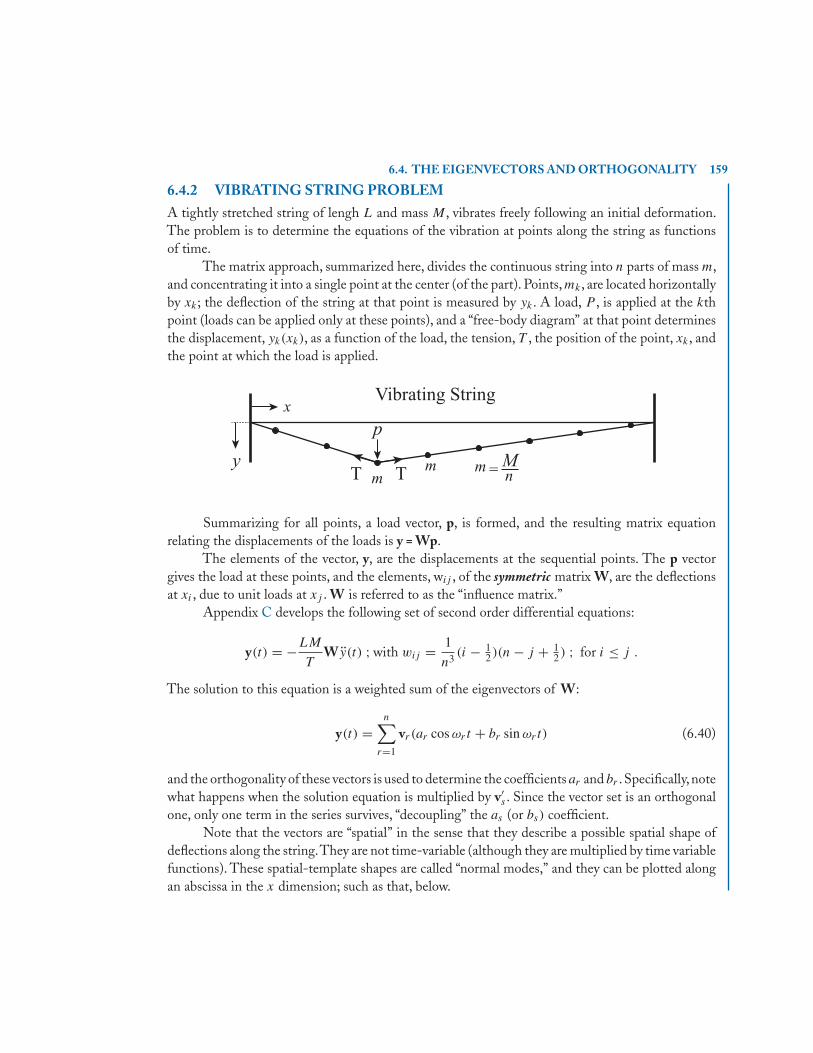
6.4. THE EIGENVECTORS AND ORTHOGONALITY 159
6.4.2 VIBRATING STRING PROBLEMA tightly stretched string of lengh L and mass M , vibrates freely following an initial deformation.The problem is to determine the equations of the vibration at points along the string as functionsof time.
The matrix approach, summarized here, divides the continuous string into n parts of mass m,and concentrating it into a single point at the center (of the part). Points, mk , are located horizontallyby xk ; the deflection of the string at that point is measured by yk . A load, P , is applied at the kthpoint (loads can be applied only at these points), and a “free-body diagram” at that point determinesthe displacement, yk(xk), as a function of the load, the tension, T , the position of the point, xk , andthe point at which the load is applied.
Summarizing for all points, a load vector, p, is formed, and the resulting matrix equationrelating the displacements of the loads is y = Wp.
The elements of the vector, y, are the displacements at the sequential points. The p vectorgives the load at these points, and the elements, wij , of the symmetric matrix W, are the deflectionsat xi , due to unit loads at xj . W is referred to as the “influence matrix.”
Appendix C develops the following set of second order differential equations:
y(t) = −LM
TWy(t) ; with wij = 1
n3(i − 1
2 )(n − j + 12 ) ; for i ≤ j .
The solution to this equation is a weighted sum of the eigenvectors of W:
y(t) =n∑
r=1
vr (ar cos ωrt + br sin ωrt) (6.40)
and the orthogonality of these vectors is used to determine the coefficients ar and br .Specifically,notewhat happens when the solution equation is multiplied by v′
s . Since the vector set is an orthogonalone, only one term in the series survives, “decoupling” the as (or bs) coefficient.
Note that the vectors are “spatial” in the sense that they describe a possible spatial shape ofdeflections along the string.They are not time-variable (although they are multiplied by time variablefunctions). These spatial-template shapes are called “normal modes,” and they can be plotted alongan abscissa in the x dimension; such as that, below.
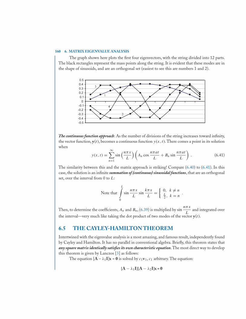
160 6. MATRIX EIGENVALUE ANALYSIS
The graph shown here plots the first four eigenvectors, with the string divided into 12 parts.The black rectangles represent the mass points along the string. It is evident that these modes are inthe shape of sinusoids, and are an orthogonal set (easiest to see this are numbers 1 and 2).
The continuous function approach: As the number of divisions of the string increases toward infinity,the vector function, y(t), becomes a continuous function y(x, t). There comes a point in its solutionwhen
y(x, t) =∞∑
n=1
sin(nπx
L
)(An cos
nπat
L+ Bn sin
nπat
L
). (6.41)
The similarity between this and the matrix approach is striking! Compare (6.40) to (6.41). In thiscase, the solution is an infinite summation of (continuous) sinusoidal functions, that are an orthogonalset, over the interval from 0 to L:
Note that
L∫0
sinnπx
Lsin
kπx
L={
0, k �= nL2 , k = n
.
Then, to determine the coefficients, An and Bn, (6.39) is multiplied by sinnπx
Land integrated over
the interval—very much like taking the dot product of two modes of the vector y(t).
6.5 THE CAYLEY-HAMILTON THEOREMIntertwined with the eigenvalue analysis is a most amazing, and famous result, independently foundby Cayley and Hamilton. It has no parallel in conventional algebra. Briefly, this theorem states thatany square matrix identically satisfies its own characteristic equation. The most direct way to developthis theorem is given by Lanczos [3] as follows:
The equation [A – λ1I]x = 0 is solved by c1v1, c1 arbitrary. The equation:
[A − λ1I][A − λ2I]x = 0
6.5. THE CAYLEY-HAMILTON THEOREM 161
is solved by x = c1v1 + c2v2 (i.e., any linear combination of v1 and v2):
[A − λ1I][A − λ2I](c1v1 + c2v2) = [A − λ1I][A − λ2I]c1v1 + [A − λ1I][A − λ2I]c2v2 .
The second term is obviously zero. The first term:
[A − λ1I][A − λ2I]c1v1 = c1[A − λ1I](Av1 − λ2v1)
= c1[A − λ1I](λ1v1 − λ2v1) .
Which is also obviously zero. Using this same reasoning, adding one more term at each step, we seethat
(A − λ1I)(A − λ2I)(A − λ3I) · · · (A − λnI)x = 0
is satisfied by any linear combination of all the eigenvectors. But, these vectors are linearly indepen-dent, and they fill the n-space.Thus, any vector at all can be represented by such a linear combination.Then every n-dimensional vector satisfies this equation. The only way that this could occur is thatthe equation is an identity.
(A − λ1I)(A − λ2I)(A − λ3I) · · · (A − λnI) ≡ 0 identically . (6.42)
It must be noted here that this proof assumes that the matrix A has a full set of eigenvectors. Forsome “defective” matrices (that are non-symmetric, and have repeated eigenvalues), a full set doesnot exist. However, it has been proven, via a limiting process, that even in the defective case, theCayley-Hamilton theorem is still true. It should also be mentioned that not all non-symmetricmatrices, even with repeated roots, are “defective.”
From Section 6.2 above, given the matrix, A, the determinant of [A – λI] expands to thecharacteristic equation:
f (λ) = c0λn + c1λ
n−1 + · · · + cn−1λ + cn = 0 . ((6.6)rewrite)
The Cayley Hamilton theorem states that:
f (A) = c0An + c1An−1 + · · · + cn−1A + cnI ≡ [0] . (6.43)
An amazing and powerful theorem. For example, by multiplying through by A−1
c0An−1 + c1An−2 + · · · + cn−1I + cnA−1 = [0] .
ThenA−1= (c0An−1+c1An−2 + · · · + cn−1I)/cn . (6.44)
By the same reasoning (6.43) shows that any power of A(nXn) can be represented in terms of powersof A no greater than n − 1. For example, the A matrix shown here is that which was used in theprevious eigenvalue analysis, the characteristic equation was:
f (λ) = λ3 − 7λ − 6 = 0 .
162 6. MATRIX EIGENVALUE ANALYSIS
Then
A3 = 7A + 6IA4 = 7A2 + 6A, andA5 = 7A3 + 6A2 = 6A2 + 49A + 42I .
Any power of this A is a function of the A matrix raised to powers no greater than 2, and the unitmatrix. Using the given A matrix, try it!
A =⎡⎣ 25 −44 18
12 −21 8−3 6 −4
⎤⎦ .
The eigenvalue analysis and Cayley Hamilton theorem also provide the solution to the analysisof A−1. Define B as A−1. Now premultiply (6.43) by Bn
f (B) = c0I + c1B + · · · + cn−1Bn−1 + cn Bn = [0] . (6.45)
Then the characteristic polynomial for B has the same coefficients as that for A, except in reverseorder—and therefore its roots are the reciprocals of those of f (A) (see the Appendix B, “Polynomi-als”). But are the eigenvectors of B the same as those of A? By definition, BA = I. Now assume thatB has the same eigenvectors, and set B = V�b U (A =V�aU has already been shown to be true).The matrices �a and �b are the eigenvalue matrices of A and B.
BA = V�bUA = (V�bU) (V�aU) = (V�b) (�aU) = VU = I . (6.46)
Since this product does produce the unit matrix, and since the inverse of A must be unique, it followsthat B = V�bU is that inverse—i.e., that the eigenvectors of B are the same as those of A, and theeigenvalues are the reciprocals.
The calculations involved in an eigenvalue analysis are at least as complex as those involvedin the inversion process. Therefore, it is unlikely that an eigenvalue analysis would ever be done justto determine A−1. Perhaps it might be useful when A is very nearly singular.
6.5.1 FUNCTIONS OF A SQUARE MATRIXThis discussion makes frequent use of the transforms defined by the eigenvalue problem and istherefore limited to square matrices, A, which have a full complement of eigenvectors.
Note that A = V�U, and A2 = (V�U)(V�U) = V�2U. Extending this
An = V�nU (6.47)
which shows that the eigenvectors of An are the same as those for A, and the eigenvalues are thenth power of those of A. This same argument holds for any polynomial in A.
P(A) = c0An + c1An−1 + · · · + cn−1A + cn (6.48)
6.5. THE CAYLEY-HAMILTON THEOREM 163
by transforming A = V�U, the polynomial, P (A) is diagonalized to P (�). Then P (A) also has theeigenvectors of A, and its j th eigenvalue equals P(λj ), where λj is the j th eigenvalue of A. Anexample is shown above for P(A) = A5. In addition, if (6.48) is postmultiplied by vk , and sinceAkvk = λkvk :
P(A)vk = P(λk)vk . (6.49)
General Polynomial FnctionsThe algebraic effort involved in actually expressing P(A) in terms of the lower degrees of A can bedaunting. The following development will help a great deal. Note, here that the general polynomialis given as P (i.e., upper case), while the characteristic polynomial will be denoted p (lower case).Then, first divide P by p. The result will be a quotient, Q, and a remainder, R:
P(x)
p(x)= Q(x)+R(x)
p(x); Then P(x) = p(x)Q(x) + R(x) and therefore: (6.50)
P(A) = p(A)Q(A) + R(A) .
But, p(A) is identically equal to zero, by the Cayley-Hamilton theorem. So, P (A) = R(A). A simpleexample is when x5 is divided by p(x), the characteristic polynomial for the example matrix at thebeginning of Section 6.5. The remainder is 6x2 + 49x + 42, which is consistent with the A5 givenabove.
For a formidable-looking example, find P (A), where P(x) given below, and A is the samematrix
P(x) = x6 − x5 − 7x4 + 31x3 + 40x2 − 19x + 5 .
The bulk of the work can be done before A is inserted. Just use synthetic division to divide P(x) bythe characteristic polynomial, p(x) = x3 – 7x – 6, and then retain the remainder, 10x2 – 5x +17.
P(A) = 10A2 − 5A + 17I .
This method, is handy, easy to use for polynomial functions. It can be extended beyond matric func-tions to analytic functions. However, its extension involves the Lagrange polynomials (see Chapter 4,Section 4.5) and arrives at the same method that is to be discussed next.
6.5.2 SYLVESTER’S THEOREMGeneral functions of A. This method is directly related to the Lagrange interpolation method, andcould possibly be deduced from it. To derive it, first define the characteristic polynomial as p(λ),and then consider the polynomial, pk(λ):
pk(λ) =n∏
j �=k
(λ − λj ); for example p1(λ) = (λ − λ2)(λ − λ3) · · · (λ − λn)
164 6. MATRIX EIGENVALUE ANALYSIS
which contains all the factors in p(λ) except (λ – λk). For the A matrix shown, p1(λ) = (λ + 2)(λ −3). Then:
pk(A) =n∏
j �=k
(A − λj I) . (6.51)
For the A matrix given here, p1(A) = (A + 2I)(A − 3I), and in the general (nXn) case, there willbe n – 1 (A – λI) terms. Each pk will be a polynomial of degree n − 1.
A =⎡⎣ 25 −44 18
12 −21 8−3 6 −4
⎤⎦
Note that pk(A)vj = 0, except when j = k, as was shown in the development of the Cayley-Hamilton theorem. And when j = k (in the example 3X3)
p1(A)v1 = (A + λ2I)(A − λ3I)v1 = (λ1 − λ2)(λ1 − λ3)v1 .
(To derive this, use the fact that Av1 = λ1v1.)
In general: pk(A)vk = vk
∏j �=k
(λk − λj ) . (6.52)
Now, define the problem: Given a general polynomial, P (A), determine a set of n coefficients ck ,such that
P(A) =n∑
k=1
ckpk(A) . (6.53)
Now, just postmultiply successively by vj (j = 1, 2, , n). When j = k: and P(A)vk = P(λk)vk
P (λk)vk = ck
∏j �=k
(λk − λj )vk and solving for ck :
ck = P(λk)∏j �=k
(λk − λj ). (6.54)
Plugging these constants back into (6.53), with the definitions of the pk(A) polynomials:
P(A) =n∑k
P (λk)
∏j �=k
(A − λj I)
∏j �=k
(λk − λj ). (6.55)
The ratios of product factors are often referred to as Zk(A), and (6.55) is written
P(A) =n∑k
P (λk)Zk(A) . (6.56)
6.6. MECHANICS OF THE EIGENVALUE PROBLEM 165
The foregoing development assumes distinct eigenvalues . In (6.55) the numerator terms are theadjoint of the matrix A(λ) = [A – λI], and the denominator is the derivative of p(λ) evaluated atλk . The equation can be generalized, and rewritten as:
F(A) =n∑
k=1
F(λk)Aa(λk)
p′(λk)(6.57)
where it is known as Sylvester’s Theorem. Equations (6.56) and (6.57) are more different than theyappear. The function F can be any analytic function, and Aa is the adjoint of [A – λI] whether ornot it has repeated roots (and the function p also represents the lowest degree polynomial satisfiedby A). Thus, Sylvester’s Theorem is more general than (6.56).
When the matrix, A, has distinct eigenvalues Equations (6.55) and (6.57) are the same. Thatis
Aa(λk) =n∏
j �=k
(A − λj I) and p′(λk) =n∏
j �=k
(λk − λj )
and (6.56) will be extended into analytic functions which possess an infinite series expansion. Thequestion of convergence will not be addressed. However, the series themselves converge, and theCayley-Hamilton theorem says that any sub-series of terms can be written in terms of a polynomialof degree n − 1. Therefore, convergence will be assumed.
Then the matrix series eA =∞∑
k=0
Ak
k! is a valid equation. Suppose A is 3X3. Then
Z1 = (A − λ2I)(A − λ3I)(λ1 − λ1)(λ1 − λ3)
; Z2 = (A − λ1I)(A − λ3I)(λ2 − λ1)(λ2 − λ3)
; and Z3 = (A − λ2I)(A − λ3I)(λ3 − λ1)(λ3 − λ2)
and eA = eλ1Z1 + eλ2Z2 + eλ3Z3 . (6.58)
It will take a lot of algebraic manipulation to “condense” Equation (6.58) into a single matrix; butnote that it’s just algebra. The usual phrase here is “This will be left as an exercise for the student.”
6.6 MECHANICS OF THE EIGENVALUE PROBLEMEfficient eigenvalue analysis is a problem in numerical analysis—beyond the scope of this work.Thesteps described below are those that illustrate the problem and the matrix characteristics. They are
• Determine the characteristic equation (calculation of the polynomial coefficients).
• Factor the characteristic equation, to obtain the eigenvalues, λi .
• For each value, λi , find the corresponding eigenvectors.
In a later section, a more sophisticated method is presented, which cleverly transforms thegiven matrix into one whose eigenvalues and eigenvectors are easily calculated—even when theseare complex numbers. Known as Danilevsky’s method, it is far superior to these methods for realisticmatrices. And, even so, there may be methods that are superior to Danilevsky’s.
166 6. MATRIX EIGENVALUE ANALYSIS
6.6.1 CALCULATING THE CHARACTERISTIC EQUATION COEFFICIENTSPipes1 reports that Maxime Bôcher has shown that the coefficients are related to the “traces” (sumof the diagonal elements) of the powers of the input matrix, A. Let Sj denote the trace of the ithpower of A:
S1 = Trace[A] = Tr[A], S2 = Trace[A2], . . . Sn = Trace[An]then the coefficients, ck , of the characteristic Equation (6.6) are calculated successively, as follows:
c0 = 1c1 = −S1
c2 = −(c1S1 + S2)2; and, in general:ck = −(ck−1S1 + ck−2S2) + . . . + c1Sk−1 + Sk)/k (6.59)
This relationship is easily programmed, providing an easy method for developing p(λ). Also,the powers of the A matrix can be saved to be used later (in determining the adjoints, Aa(λi)).
6.6.2 FACTORING THE CHARACTERISTIC EQUATIONThere are handbook methods for factoring polynomials up to degree 4.Although there will not be anyexamples herein resulting in p(λ) of higher degree, Appendix B,“Polynomials,” discusses polynomialarithmetic and outlines computer methods, including root determination, real or complex.
Finding the roots of a polynomial requires a computer; and the computer routines for poly-nomial manipulation are very simple. See Appendix B.
6.6.3 CALCULATION OF THE EIGENVECTORSUsing Gauss-Jordan ReductionThe matrix [A − λj I] is singular, and in this discussion will be assumed to have rank n − 1.Then, theGauss-Jordan is an excellent tool to derive the eigenvectors one at a time.The method is described inSection 3.3. A 4X4 will be used in illustration from the point at which the Gauss-Jordan reductionof [A − λj I] terminates. If A(λj ) is complex, the reduction must be done in a complex arithmetic.
∥∥∥∥∥∥∥∥1 0 0 z1
0 1 0 z2
0 0 1 z3
0 0 0 0
∥∥∥∥∥∥∥∥The reduced matrix will appear as in the diagram. If λj is complex, then the “z” values shown
here will be complex. There will be a complete row of zero values along the bottom, showing that asolution {x1, x2, x3, x4} does exist, with the value for x4 chosen arbitrarily, say k.
1See [4], page 90.
6.6. MECHANICS OF THE EIGENVALUE PROBLEM 167
The complete solution is: x1 =
⎧⎪⎪⎨⎪⎪⎩
−z1
−z2
−z3
1
⎫⎪⎪⎬⎪⎪⎭ k.
The reduction/solution will have to be repeated for each eigenvalue, and again for the transposedmatrix to obtain the row eigenvectors.
Calculation of the Adjoint of [A – λj I]This method has been shown in an earlier example. It derives both the row and column eigenvectorstogether.
From the Cayley-Hamilton theorem, denoting the characteristic equation as p(λ) = 0:
p(A) = [A − λ1I][A − λ2I] · · · [A − λnI] = [0] .
Since the numbering of the eigenvalues is arbitrary, we can write the ith term first in the above, andthen gather the rest of the product terms into a polynomial, pi :
[A - λiI]pi(A) = [0] (6.60)
where pi(A) =n∏
k �=i
[A - λkI]; (n − 1 product terms).
Since A(λi)Aa(λi) = |A(λi)|I = [0], and comparing this to (6.60), note that pi(A) is the adjointof A(λi). pi(A) will not be null, as long as λi is distinct—not a repeated root of the characteristicequation. Therefore, pi(A) will be the source of the eigenvectors.
pi can be found by synthetic division of p(λ). If the synthetic division is done in complexarithmetic, then pi(λ) is found by the synthetic division of p(λ) by (λ − λi). If the division routineaccepts only reals, and λi is complex, (a + jb), then its conjugate is also a root and the divisor canbe the quadratic, λ2 + 2aλ + a2 + b2.
The result of this division must then be multiplied by (λ − a + jb):
pi(λ) = P(λ)
λ2 + 2aλ + a2 + b2× (λ − a + jb) (6.61)
When pi(λ) has been found, matrix multiplications are then needed to derive pi(A) = Aa(λi).This method of determining the adjoint of [A - λiI], containing the eigenvectors, has the
advantage that operations with complex numbers are minimized. Only the final multiplication by[A − (a + jb)I] involves complex arithmetic.The powers of the original matrix are available, havingbeen calculated for defining the coefficients of the characteristic polynomial.
When the initial row, x, and column, z, vectors have been determined (in general complexnumbers), they must be normalized—usually such that xj•zi = 1—defining vj and ui .
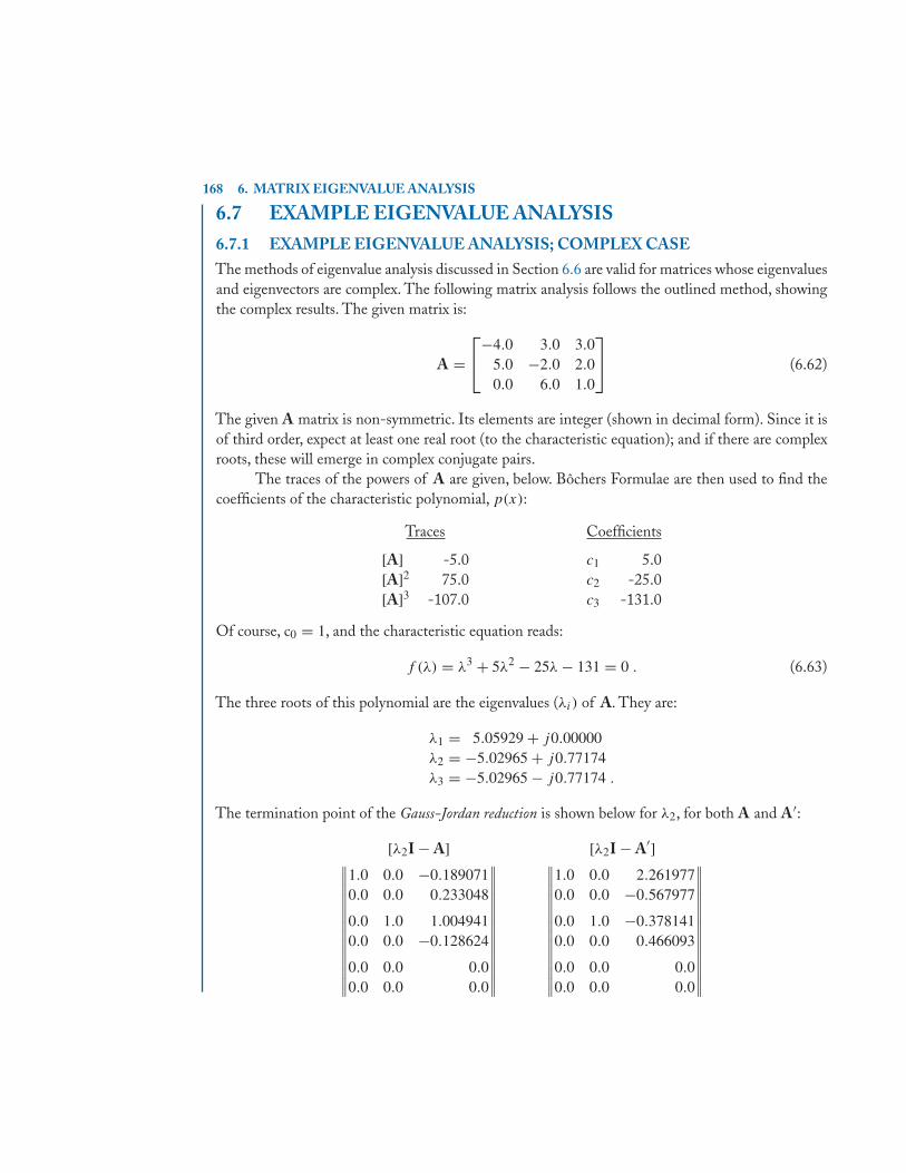
168 6. MATRIX EIGENVALUE ANALYSIS
6.7 EXAMPLE EIGENVALUE ANALYSIS6.7.1 EXAMPLE EIGENVALUE ANALYSIS; COMPLEX CASEThe methods of eigenvalue analysis discussed in Section 6.6 are valid for matrices whose eigenvaluesand eigenvectors are complex. The following matrix analysis follows the outlined method, showingthe complex results. The given matrix is:
A =⎡⎣−4.0 3.0 3.0
5.0 −2.0 2.00.0 6.0 1.0
⎤⎦ (6.62)
The given A matrix is non-symmetric. Its elements are integer (shown in decimal form). Since it isof third order, expect at least one real root (to the characteristic equation); and if there are complexroots, these will emerge in complex conjugate pairs.
The traces of the powers of A are given, below. Bôchers Formulae are then used to find thecoefficients of the characteristic polynomial, p(x):
Traces Coefficients
[A] -5.0 c1 5.0[A]2 75.0 c2 -25.0[A]3 -107.0 c3 -131.0
Of course, c0 = 1, and the characteristic equation reads:
f (λ) = λ3 + 5λ2 − 25λ − 131 = 0 . (6.63)
The three roots of this polynomial are the eigenvalues (λi) of A. They are:
λ1 = 5.05929 + j0.00000λ2 = −5.02965 + j0.77174λ3 = −5.02965 − j0.77174 .
The termination point of the Gauss-Jordan reduction is shown below for λ2, for both A and A′:
[λ2I − A] [λ2I − A′]∥∥∥∥∥∥∥∥∥∥∥∥∥∥
1.0 0.0 −0.1890710.0 0.0 0.233048
0.0 1.0 1.0049410.0 0.0 −0.128624
0.0 0.0 0.00.0 0.0 0.0
∥∥∥∥∥∥∥∥∥∥∥∥∥∥
∥∥∥∥∥∥∥∥∥∥∥∥∥∥
1.0 0.0 2.2619770.0 0.0 −0.567977
0.0 1.0 −0.3781410.0 0.0 0.466093
0.0 0.0 0.00.0 0.0 0.0
∥∥∥∥∥∥∥∥∥∥∥∥∥∥
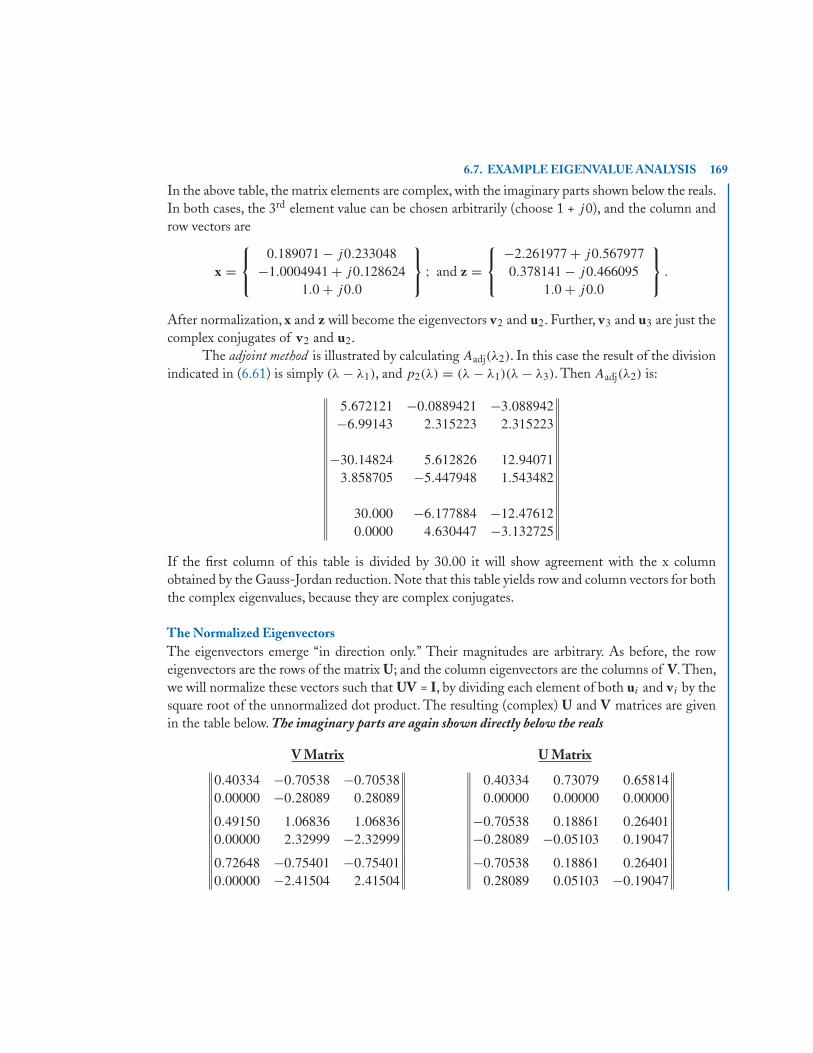
6.7. EXAMPLE EIGENVALUE ANALYSIS 169
In the above table, the matrix elements are complex, with the imaginary parts shown below the reals.In both cases, the 3rd element value can be chosen arbitrarily (choose 1 + j0), and the column androw vectors are
x =⎧⎨⎩
0.189071 − j0.233048−1.0004941 + j0.128624
1.0 + j0.0
⎫⎬⎭ ; and z =
⎧⎨⎩
−2.261977 + j0.5679770.378141 − j0.466095
1.0 + j0.0
⎫⎬⎭ .
After normalization, x and z will become the eigenvectors v2 and u2. Further, v3 and u3 are just thecomplex conjugates of v2 and u2.
The adjoint method is illustrated by calculating Aadj(λ2). In this case the result of the divisionindicated in (6.61) is simply (λ − λ1), and p2(λ) = (λ − λ1)(λ − λ3). Then Aadj(λ2) is:∥∥∥∥∥∥∥∥∥∥∥∥∥∥∥∥∥
5.672121 −0.0889421 −3.088942−6.99143 2.315223 2.315223
−30.14824 5.612826 12.940713.858705 −5.447948 1.543482
30.000 −6.177884 −12.476120.0000 4.630447 −3.132725
∥∥∥∥∥∥∥∥∥∥∥∥∥∥∥∥∥If the first column of this table is divided by 30.00 it will show agreement with the x columnobtained by the Gauss-Jordan reduction. Note that this table yields row and column vectors for boththe complex eigenvalues, because they are complex conjugates.
The Normalized EigenvectorsThe eigenvectors emerge “in direction only.” Their magnitudes are arbitrary. As before, the roweigenvectors are the rows of the matrix U; and the column eigenvectors are the columns of V. Then,we will normalize these vectors such that UV = I, by dividing each element of both ui and vi by thesquare root of the unnormalized dot product. The resulting (complex) U and V matrices are givenin the table below. The imaginary parts are again shown directly below the reals
V Matrix U Matrix∥∥∥∥∥∥∥∥∥∥∥∥∥∥
0.40334 −0.70538 −0.705380.00000 −0.28089 0.28089
0.49150 1.06836 1.068360.00000 2.32999 −2.32999
0.72648 −0.75401 −0.754010.00000 −2.41504 2.41504
∥∥∥∥∥∥∥∥∥∥∥∥∥∥
∥∥∥∥∥∥∥∥∥∥∥∥∥∥
0.40334 0.73079 0.658140.00000 0.00000 0.00000
−0.70538 0.18861 0.26401−0.28089 −0.05103 0.19047
−0.70538 0.18861 0.264010.28089 0.05103 −0.19047
∥∥∥∥∥∥∥∥∥∥∥∥∥∥
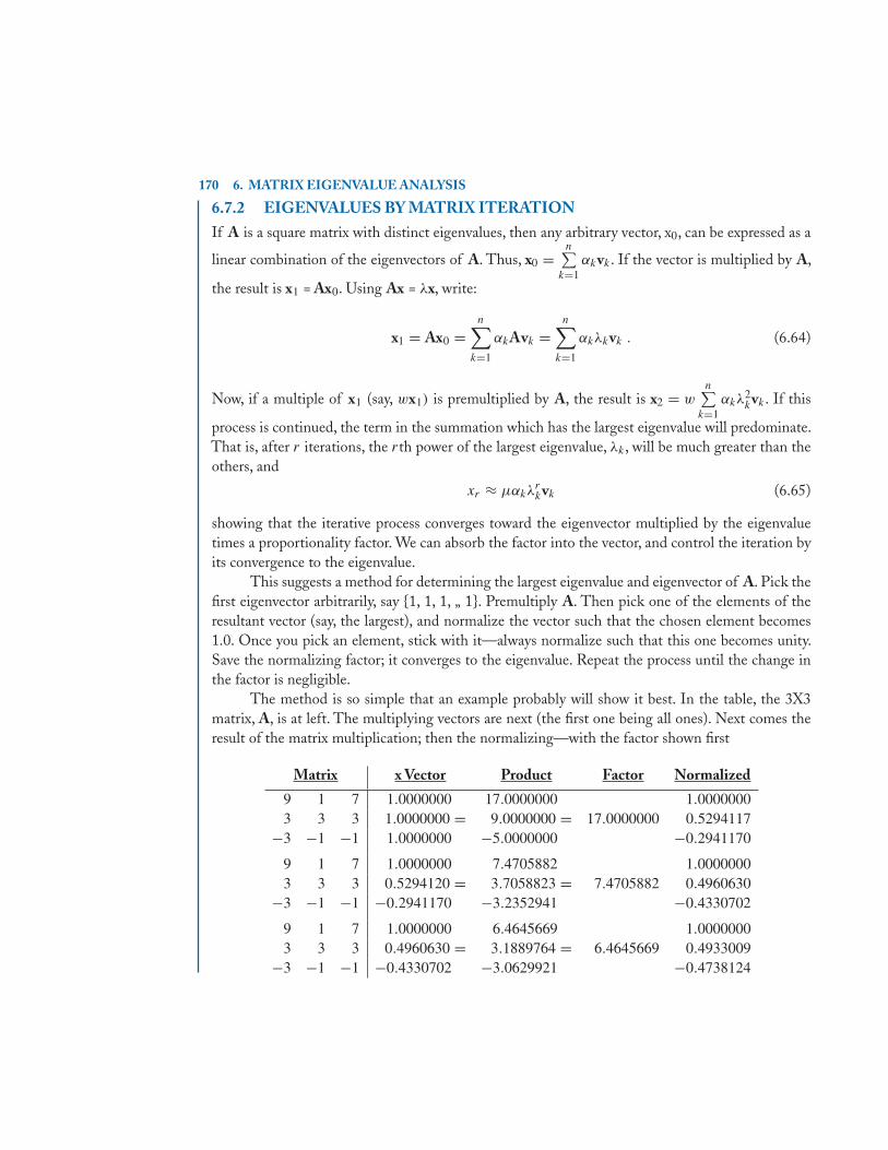
170 6. MATRIX EIGENVALUE ANALYSIS
6.7.2 EIGENVALUES BY MATRIX ITERATIONIf A is a square matrix with distinct eigenvalues, then any arbitrary vector, x0, can be expressed as a
linear combination of the eigenvectors of A. Thus, x0 =n∑
k=1αkvk . If the vector is multiplied by A,
the result is x1 = Ax0. Using Ax = λx, write:
x1 = Ax0 =n∑
k=1
αkAvk =n∑
k=1
αkλkvk . (6.64)
Now, if a multiple of x1 (say, wx1) is premultiplied by A, the result is x2 = wn∑
k=1αkλ
2kvk . If this
process is continued, the term in the summation which has the largest eigenvalue will predominate.That is, after r iterations, the rth power of the largest eigenvalue, λk , will be much greater than theothers, and
xr ≈ μαkλrkvk (6.65)
showing that the iterative process converges toward the eigenvector multiplied by the eigenvaluetimes a proportionality factor. We can absorb the factor into the vector, and control the iteration byits convergence to the eigenvalue.
This suggests a method for determining the largest eigenvalue and eigenvector of A. Pick thefirst eigenvector arbitrarily, say {1, 1, 1, „ 1}. Premultiply A. Then pick one of the elements of theresultant vector (say, the largest), and normalize the vector such that the chosen element becomes1.0. Once you pick an element, stick with it—always normalize such that this one becomes unity.Save the normalizing factor; it converges to the eigenvalue. Repeat the process until the change inthe factor is negligible.
The method is so simple that an example probably will show it best. In the table, the 3X3matrix, A, is at left. The multiplying vectors are next (the first one being all ones). Next comes theresult of the matrix multiplication; then the normalizing—with the factor shown first
Matrix x Vector Product Factor Normalized
9 1 7 1.0000000 17.0000000 1.00000003 3 3 1.0000000 = 9.0000000 = 17.0000000 0.5294117
−3 −1 −1 1.0000000 −5.0000000 −0.2941170
9 1 7 1.0000000 7.4705882 1.00000003 3 3 0.5294120 = 3.7058823 = 7.4705882 0.4960630
−3 −1 −1 −0.2941170 −3.2352941 −0.4330702
9 1 7 1.0000000 6.4645669 1.00000003 3 3 0.4960630 = 3.1889764 = 6.4645669 0.4933009
−3 −1 −1 −0.4330702 −3.0629921 −0.4738124
6.8. THE EIGENVALUE ANALYSIS OF SIMILAR MATRICES; DANILEVSKY’S METHOD 171
In the example shown, if the iterations were continued, the eigenvalue would emerge as 6.00 andthe eigenvector converges to {1.0, 0.5, −0.5}.Note: this matrix is not symmetric. It could therefore have had complex eigenvalues and vectors. Inthat case, the convergence is quite different. Although iteration does work for the complex case, itwill not be discussed here. Even if the eigenvalues and vectors are real, it is necessary to transpose Aand iterate for the row eigenvector (the eigenvalue will be the same).
If it is desired to continue the procedure for the next largest eigenvalue—vector, then the newmatrix is formed by subtracting out the results of the first iteration: B = A − λ1v1u1. As in anyiterative procedure, it is necessary to keep many significant figures. Even then, only the first “few”results will be within acceptable accuracy. Usually iteration is only done on large symmetric matrices,and only to derive the first one or two eigenvalues—vectors.
6.8 THE EIGENVALUE ANALYSIS OF SIMILAR MATRICES;DANILEVSKY’S METHOD
The eigenvalue analysis of a matrix has always been considered formidable, especially before thedigital computer was available to do the messy calculations. It is no surprise, therefore, to find thatmethods have been developed to shorten and simplify the work. In the present day, the best of thesemethods are those that are coded easily on the computer. A method will be discussed which uses a“similarity transform” to develop a new matrix whose eigenvalue analysis is very simple to perform.And in this case, the matrix transformation, somewhat analogous to the Gauss-Jordan reductionmethod in determinants, is not a difficult one.
In Chapter 5, Section 5.4, the subject of “similar” matrices is introduced. In particular, twomatrices, say A and P, are defined as being “similar” if there exists a relation:
A = SPS−1 . (6.66)
That is, the pre- and postmultiplying transform matrices are inverses of one another. Of specialinterest at present is the fact that similar matrices are possessed of the same eigenvalues. To showthis we begin with the Cayley-Hamilton equation for A:
(A − λ1I)(A − λ2I)(A − λ3I) · · · (A − λnI)v = 0 . (6.67)
We can substitute A from (6.66) into (6.67)
(SPS−1 − λ1I)(SPS−1 - λ2I)(SPS−1 − λ3I)· · ·(SPS−1 − λnI)v = 0
and since I = SS−1:
(SPS−1 − λ1SS−1)(SPS−1 − λ2SS−1)(SPS−1 − λ3SS−1) · · · (SPS−1 − λnSS−1)v = 0S(P − λ1I)(P − λ2I)(P − λ3I) · · · (P − λnI)S−1v= 0
(P − λ1I)(P − λ2I)(P − λ3I) · · · (P − λnI)x = 0; x = S−1v . (6.68)
172 6. MATRIX EIGENVALUE ANALYSIS
(6.68) clearly shows the same Cayley-Hamilton equation, with the same eigenvalues, as (6.67).Of course, there are infinities of similarity transforms. The trick is to find one in which the
analysis of the P matrix is easier to perform than the analysis of the original A.In Danilevsky’s method this is definitely the case.
6.8.1 DANILEVSKY’S METHODThe objective of this method is to derive, from the given input A matrix, the similar P matrix:
P =
⎡⎢⎢⎣
p11 p12 p13 p14
1 0 0 00 1 0 00 0 1 0
⎤⎥⎥⎦ .
In the above, and some of the displays that follow, a 4X4 will be shown, in preference to writing outa completely general case. The 4X4 will be clearer to follow (extension to nXn should be obvious).
Note that the unity elements are not on the main diagonal – but, are one diagonal down.All of the data in the original A matrix has been “squeezed” into the elements of the first row. Inorder to derive the characteristic equation, we subtract λ from the main diagonal and solve for thedeterminant. This is most easily done by expanding in minors of the first row. The result:
f (λ) = λn − p11λn−1 … − p1,n−1λ − p1n = 0, in general (6.69)
f (λ) = λ4 − p11λ3 − p12λ
2 − p13λ − p14 = 0, in the 4X4 .
That is, the first row elements of P are none other than the (negatives of ) the characteristic equationcoefficients. We are assured that the eigenvalues of P are the same as those of A, by the argumentabove.We must therefore conclude that the characteristic equation is the same, and is given by (6.69).Once the characteristic equation is derived, a separate method is used to determine the eigenvalues, theroots of the polynomial.
Since P appears so very different from A, it would seem that the transform would be a verycomplex one. But, that is not the case. The transform is affected sequentially by a series of verysimple matrices, M−1
k−1 and Mk−1, where k takes on the values n, n-1, …, 2, (n being the order ofA). Note that the M matrices are required to be inverses.
Then, the first transform will be An−1 = M−1n−1AMn−1. Next, transform An−1, An−2, etc.:
An−2 = M−1n−2An−1Mn−2 = M−1
n−2(M−1n−1AMn−1)Mn−2
An−3 = M−1n−3An−2Mn−3 = M−1
n−3(M−1n−2(M−1
n−1AMn−1)Mn−2)Mn−3
until finally
⎧⎪⎨⎪⎩
P = S−1AS = M−11 M−1
2 · · · M−1n−1[A]Mn−1 · · · M2M1
S−1 =n−1∏k=1
M−1k ; and S =
1∏k=n−1
M−1k .
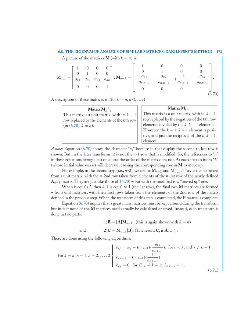
6.8. THE EIGENVALUE ANALYSIS OF SIMILAR MATRICES; DANILEVSKY’S METHOD 173
A picture of the matrices M (with k = n) is:
M−1n−1 =
⎡⎢⎢⎢⎣
1 0 0 00 1 0 0
an1 an2 an3 ann
0 0 0 1
⎤⎥⎥⎥⎦ ; Mn−1 =
⎡⎢⎢⎢⎢⎢⎣
1 0 0 00 1 0 0
− an1
an,n−1− an2
an,n−1+ 1
an,n−1− ann
an,n−1
0 0 0 1
⎤⎥⎥⎥⎥⎥⎦ .
(6.70)A description of these matrices is: (for k = n, n-1, …2)
Matrix M−1k−1
This matrix is a unit matrix, with its k − 1row replaced by the elements of the kth row(in (6.70), k = n).
Matrix Mk−1
This matrix is a unit matrix, with its k − 1row replaced by the negatives of the kth rowelements divided by the k, k − 1 element.However, the k − 1, k − 1 element is posi-tive, and just the reciprocal of the k, k − 1element.
A note: Equation (6.70) shows the character “n,” because in that display the second to last row isshown. But, in the later transforms, it is not the n-1 row that is modified. So, the references to “n”in these equations changes, but of course the order of the matrix does not. At each step an index “k”(whose initial value was n) will decrease, causing the corresponding row in M to move up.
For example, in the second step (i.e., n-2), we define Mn−2 and M−1n−2. They are constructed
from a unit matrix, with the n-2nd row taken from elements of the n-1st row of the newly definedAn−1 matrix. They are just like those of (6.70) – but with the modified row “moved up” one.
When k equals 2, then k-1 is equal to 1 (the 1st row), the final two M matrices are formed– from unit matrices, with their first rows taken from the elements of the 2nd row of the matrixdefined in the previous step. When the transform of this step is completed, the P matrix is complete.
Equation (6.70) implies that a great many matrices must be kept around during the transform,but in fact none of the M matrices need actually be calculated or saved. Instead, each transform isdone in two parts:
1)B = [A]Mn−1; (this is again shown with k = n)
and 2)C = M−1n−1[B]. (The result, C, is An−1) .
These are done using the following algorithms:
For k = n, n − 1, n − 2, . . . , 2
⎧⎪⎪⎪⎨⎪⎪⎪⎩
bij = aij − (ai,k−1)(akj
ak,k−1), for i < k, and j �= k − 1
bi,k−1 = (ai,k−1)(1
ak,k−1)
bkj = 0, for all j �= k − 1; bk,k−1 = 1 .
(6.71)
174 6. MATRIX EIGENVALUE ANALYSIS
Note especially, the last row of B. In a 4X4, that row will be {0, 0, 1, 0}. This is already the last rowof P. Note also that the premultiplication of M−1
n−1 will not disturb the last row. In fact, the onlyrow affected by this premultiplication is the k-1st row. That is, in C = M−1
k−1[B]:⎧⎪⎨⎪⎩
cij = bij for all i �= k − 1, and all j
ck−1,j =n∑
s=1
aksbsj , for all j .(6.72)
In forming B and C, it is not necessary to actually multiply matrices. The relations shown in (6.71)and (6.72) are all that are needed. In carrying on to the next step, we simply set A equal to C, andthen proceed with k decreased by one. That is, we “move up one row.” And so it goes until k = 2.
Notice that the definition of the M matrix elements includes a division. For example, in thefirst step we divide by an,n−1. If any of these terms happens to be zero, then one must search upwardalong the n-1st column (or the “k-1st” column) to find a corresponding element that is not zero;and then interchange the two rows. This is the same as multiplying both M and M−1 by the unitmatrix, with the same two rows interchanged. Then the transform remains a similar transform, andthe development can proceed normally. In the event that no nonzero element can be found, themethod fails.
Since the Mk and M−1k matrices (i.e., those defined in Equation (6.70)) are never actually
calculated, the S and S−1 matrices will not be determined unless there is a reason to do so. If onlythe eigenvalues are required, S and S−1 are not needed. But, a complete eigenvalue analysis requiresthe vectors as well. Equation (6.68) already implies that these matrices will, then, be required.
Distinct eigenvalues. The following paragraphs outline the method for determining the eigenvectors.It will be noted that for each eigenvalue, just one pair of eigenvectors (row and column) is formed . Ifthe eigenvalues are not distinct, the method fails.
Defining the EigenvectorsReturning to the eigenvalue analysis of P; for each root, we have the following equation to solve forthe column eigenvectors: (the eigenvectors of P, are defined as x, column and z, row):⎡
⎢⎢⎣p11 − λi p12 p13 p14
1 −λi 0 00 1 −λi 00 0 1 −λi
⎤⎥⎥⎦⎧⎪⎪⎨⎪⎪⎩
x1
x2
x3
x4
⎫⎪⎪⎬⎪⎪⎭ = 0 . (6.73)
First, arbitrarily assign the value 1.0 to x4 (xn, in general). Then, using the last 3 equations (n-1equations in general), the elements of the ith x vector are:
xn = 1; xk = λxk+1, for k = n − 1, n − 2, . . . , 1 . (6.74)
For example, in the 4X4 case, xi = { λ3i , λ2
i , λi , 1 }.
6.8. THE EIGENVALUE ANALYSIS OF SIMILAR MATRICES; DANILEVSKY’S METHOD 175
For the row eigenvectors, we have [zi][P-λiI] = 0, a row equation:
[z1 z2 z3 z4
]⎡⎢⎢⎣
p11 − λi p12 p13 p14
1 −λi 0 00 1 −λi 00 0 1 −λi
⎤⎥⎥⎦ = 0. (6.75)
In this case, set z1 = 1, and then
zk = λizk−1 − p1,k−1, for k = 2, 3, . . . n . (6.76)
Because of the simplicity of P, its eigenvectors are easily derived. But, although the eigenvalues ofP are the same as those of A, the eigenvectors are different . Starting with [A-λiI]vi :
(A − λiI)vi = (SPS−1 − λiI)vi = S(P − λiI)S−1vi → (P − λiI)xi
we see that we must transform vi by S−1. That is xi = S−1vi , where x is the column vector in (6.73).Therefore, to obtain v from x, we must premultiply by S. In the row vector case, the logic is verysimilar, and the resulting transforms are:
vi = Sxi
[ui] = [zi]S−1 . (6.77)
In Equations (6.77), the square brackets are used just to emphasize that ui and zi are row vectors.Since both S and S−1 are used in the definition of the vectors, then for a complete eigenvalue analysisthese matrices must be retained as the similarity transform proceeds.
Recall, from (6.71) and (6.72), that the original A matrix is updated via the intermediatematrices, B, and C (only one of which has to be kept – i.e., C is the “in-place” update of B). In thesame sense, define a matrix, S, which will be used to update S. At the end of each update cycle, S willbe set equal to S, and the next cycle will again update S. The emerging matrix S−1 will be updatedin-place.
The relationships are very similar to those of (6.71) and (6.72):
(S, S−1, and S initialized to unit matrices)⎧⎪⎪⎪⎪⎪⎨⎪⎪⎪⎪⎪⎩
sk−1,j = − ak,j
ak,k−1, for all j �= k − 1; sk−1,k−1 = 1
ak,k−1
si,j = si,j − si,k−1 • ak,j
ak,k−1, for (k − 1) < i < n, and j �= k − 1
si,k−1 = si,k−1
ak,k−1, for (k − 1) < i < n, and j = k − 1.
(6.78)
s−1k−1,j =
n∑p=1
ak,p • s−1k,j , for all j . (6.79)
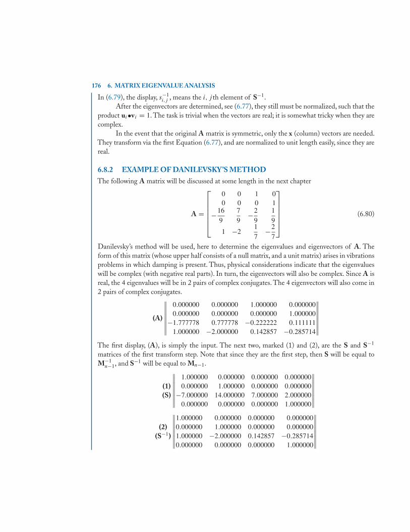
176 6. MATRIX EIGENVALUE ANALYSIS
In (6.79), the display, s−1i,j , means the i, j th element of S−1.
After the eigenvectors are determined, see (6.77), they still must be normalized, such that theproduct ui•vi = 1. The task is trivial when the vectors are real; it is somewhat tricky when they arecomplex.
In the event that the original A matrix is symmetric, only the x (column) vectors are needed.They transform via the first Equation (6.77), and are normalized to unit length easily, since they arereal.
6.8.2 EXAMPLE OF DANILEVSKY’S METHODThe following A matrix will be discussed at some length in the next chapter
A =
⎡⎢⎢⎢⎢⎢⎣
0 0 1 00 0 0 1
−16
9
7
9−2
9
1
9
1 −21
7−2
7
⎤⎥⎥⎥⎥⎥⎦ (6.80)
Danilevsky’s method will be used, here to determine the eigenvalues and eigenvectors of A. Theform of this matrix (whose upper half consists of a null matrix, and a unit matrix) arises in vibrationsproblems in which damping is present. Thus, physical considerations indicate that the eigenvalueswill be complex (with negative real parts). In turn, the eigenvectors will also be complex. Since A isreal, the 4 eigenvalues will be in 2 pairs of complex conjugates. The 4 eigenvectors will also come in2 pairs of complex conjugates.
(A)
∥∥∥∥∥∥∥∥0.000000 0.000000 1.000000 0.0000000.000000 0.000000 0.000000 1.000000
−1.777778 0.777778 −0.222222 0.1111111.000000 −2.000000 0.142857 −0.285714
∥∥∥∥∥∥∥∥The first display, (A), is simply the input. The next two, marked (1) and (2), are the S and S−1
matrices of the first transform step. Note that since they are the first step, then S will be equal toM−1
n−1, and S−1 will be equal to Mn−1.
(1)(S)
∥∥∥∥∥∥∥∥1.000000 0.000000 0.000000 0.0000000.000000 1.000000 0.000000 0.000000
−7.000000 14.000000 7.000000 2.0000000.000000 0.000000 0.000000 1.000000
∥∥∥∥∥∥∥∥(2)
(S−1)
∥∥∥∥∥∥∥∥1.000000 0.000000 0.000000 0.0000000.000000 1.000000 0.000000 0.0000001.000000 −2.000000 0.142857 −0.2857140.000000 0.000000 0.000000 1.000000
∥∥∥∥∥∥∥∥
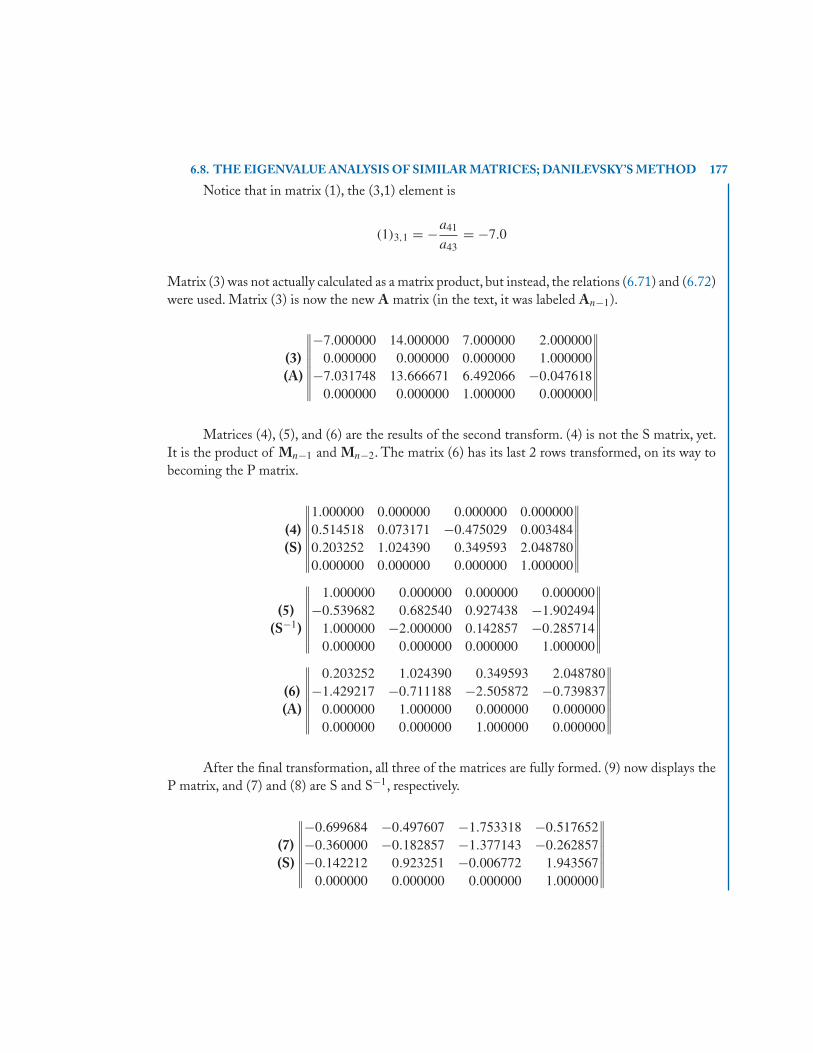
6.8. THE EIGENVALUE ANALYSIS OF SIMILAR MATRICES; DANILEVSKY’S METHOD 177
Notice that in matrix (1), the (3,1) element is
(1)3,1 = −a41
a43= −7.0
Matrix (3) was not actually calculated as a matrix product, but instead, the relations (6.71) and (6.72)were used. Matrix (3) is now the new A matrix (in the text, it was labeled An−1).
(3)(A)
∥∥∥∥∥∥∥∥−7.000000 14.000000 7.000000 2.000000
0.000000 0.000000 0.000000 1.000000−7.031748 13.666671 6.492066 −0.047618
0.000000 0.000000 1.000000 0.000000
∥∥∥∥∥∥∥∥Matrices (4), (5), and (6) are the results of the second transform. (4) is not the S matrix, yet.
It is the product of Mn−1 and Mn−2. The matrix (6) has its last 2 rows transformed, on its way tobecoming the P matrix.
(4)(S)
∥∥∥∥∥∥∥∥1.000000 0.000000 0.000000 0.0000000.514518 0.073171 −0.475029 0.0034840.203252 1.024390 0.349593 2.0487800.000000 0.000000 0.000000 1.000000
∥∥∥∥∥∥∥∥(5)
(S−1)
∥∥∥∥∥∥∥∥1.000000 0.000000 0.000000 0.000000
−0.539682 0.682540 0.927438 −1.9024941.000000 −2.000000 0.142857 −0.2857140.000000 0.000000 0.000000 1.000000
∥∥∥∥∥∥∥∥(6)(A)
∥∥∥∥∥∥∥∥0.203252 1.024390 0.349593 2.048780
−1.429217 −0.711188 −2.505872 −0.7398370.000000 1.000000 0.000000 0.0000000.000000 0.000000 1.000000 0.000000
∥∥∥∥∥∥∥∥After the final transformation, all three of the matrices are fully formed. (9) now displays the
P matrix, and (7) and (8) are S and S−1, respectively.
(7)(S)
∥∥∥∥∥∥∥∥−0.699684 −0.497607 −1.753318 −0.517652−0.360000 −0.182857 −1.377143 −0.262857−0.142212 0.923251 −0.006772 1.943567
0.000000 0.000000 0.000000 1.000000
∥∥∥∥∥∥∥∥
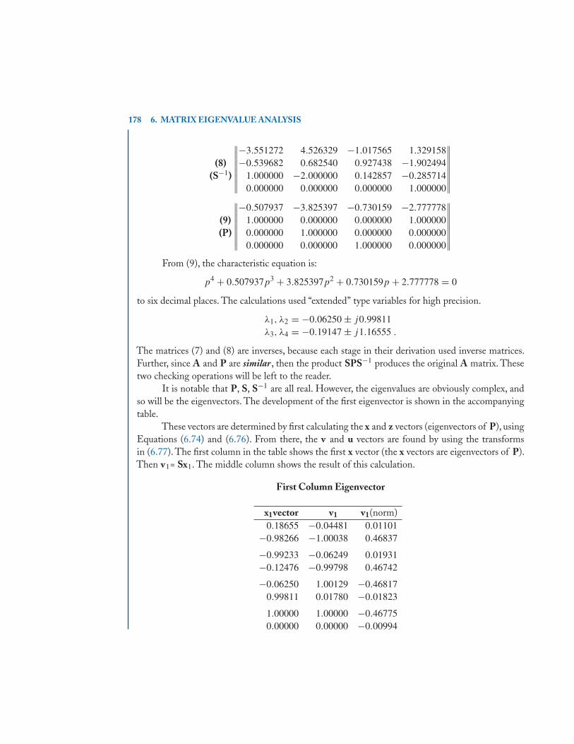
178 6. MATRIX EIGENVALUE ANALYSIS
(8)(S−1)
∥∥∥∥∥∥∥∥−3.551272 4.526329 −1.017565 1.329158−0.539682 0.682540 0.927438 −1.902494
1.000000 −2.000000 0.142857 −0.2857140.000000 0.000000 0.000000 1.000000
∥∥∥∥∥∥∥∥(9)(P)
∥∥∥∥∥∥∥∥−0.507937 −3.825397 −0.730159 −2.777778
1.000000 0.000000 0.000000 1.0000000.000000 1.000000 0.000000 0.0000000.000000 0.000000 1.000000 0.000000
∥∥∥∥∥∥∥∥From (9), the characteristic equation is:
p4 + 0.507937p3 + 3.825397p2 + 0.730159p + 2.777778 = 0
to six decimal places. The calculations used “extended” type variables for high precision.
λ1, λ2 = −0.06250 ± j0.99811λ3, λ4 = −0.19147 ± j1.16555 .
The matrices (7) and (8) are inverses, because each stage in their derivation used inverse matrices.Further, since A and P are similar, then the product SPS−1 produces the original A matrix. Thesetwo checking operations will be left to the reader.
It is notable that P, S, S−1 are all real. However, the eigenvalues are obviously complex, andso will be the eigenvectors. The development of the first eigenvector is shown in the accompanyingtable.
These vectors are determined by first calculating the x and z vectors (eigenvectors of P), usingEquations (6.74) and (6.76). From there, the v and u vectors are found by using the transformsin (6.77). The first column in the table shows the first x vector (the x vectors are eigenvectors of P).Then v1= Sx1. The middle column shows the result of this calculation.
First Column Eigenvector
x1vector v1 v1(norm)0.18655 −0.04481 0.01101
−0.98266 −1.00038 0.46837
−0.99233 −0.06249 0.01931−0.12476 −0.99798 0.46742
−0.06250 1.00129 −0.468170.99811 0.01780 −0.01823
1.00000 1.00000 −0.467750.00000 0.00000 −0.00994
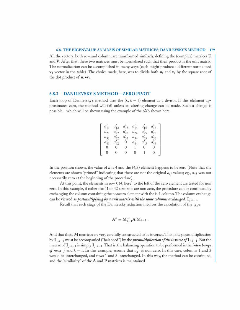
6.8. THE EIGENVALUE ANALYSIS OF SIMILAR MATRICES; DANILEVSKY’S METHOD 179
All the vectors, both row and column, are transformed similarly, defining the (complex) matrices Uand V. After that, these two matrices must be normalized such that their product is the unit matrix.The normalization can be accomplished in many ways (each might produce a different normalizedv1 vector in the table). The choice made, here, was to divide both ui and vi by the square root ofthe dot product of ui•vi .
6.8.3 DANILEVSKY’S METHOD—ZERO PIVOTEach loop of Danilevsky’s method uses the (k, k − 1) element as a divisor. If this elelment ap-proximates zero, the method will fail unless an altering change can be made. Such a change ispossible—which will be shown using the example of the 6X6 shown here.
⎡⎢⎢⎢⎢⎢⎢⎢⎣
a′11 a′
12 a′13 a′
14 a′15 a′
16a′
21 a′22 a′
23 a′24 a′
25 a′26
a′31 a′
32 a′33 a′
34 a′35 a′
36a′
41 a′42 0 a′
44 a′45 a′
460 0 0 1 0 00 0 0 0 1 0
⎤⎥⎥⎥⎥⎥⎥⎥⎦
In the position shown, the value of k is 4 and the (4,3) element happens to be zero (Note that theelements are shown “primed” indicating that these are not the original aij values; eg., a43 was notnecessarily zero at the beginning of the procedure).
At this point, the elements in row k (4, here) to the left of the zero element are tested for nonzero. In this example, if either the 41 or 42 elements are non zero, the procedure can be continued byexchanging the column containing the nonzero element with the k-1 column.The column exchangecan be viewed as postmultiplying by a unit matrix with the same columns exchanged , Ij,k−1.
Recall that each stage of the Danilevsky reduction involves the calculation of the type:
A′′ = M−1k−1A′Mk−1 .
And that these M matrices are very carefully constructed to be inverses.Then, the postmultiplicationby Ij,k−1 must be accompanied (“balanced”) by the premultiplication of the inverse of Ij,k−1. But theinverse of Ij,k−1 is simply Ij,k−1.That is, the balancing operation to be performed is the interchangeof rows j and k − 1. In this example, assume that a′
41 is non zero. In this case, columns 1 and 3would be interchanged, and rows 1 and 3 interchanged. In this way, the method can be continued,and the “similarity” of the A and P matrices is maintained.
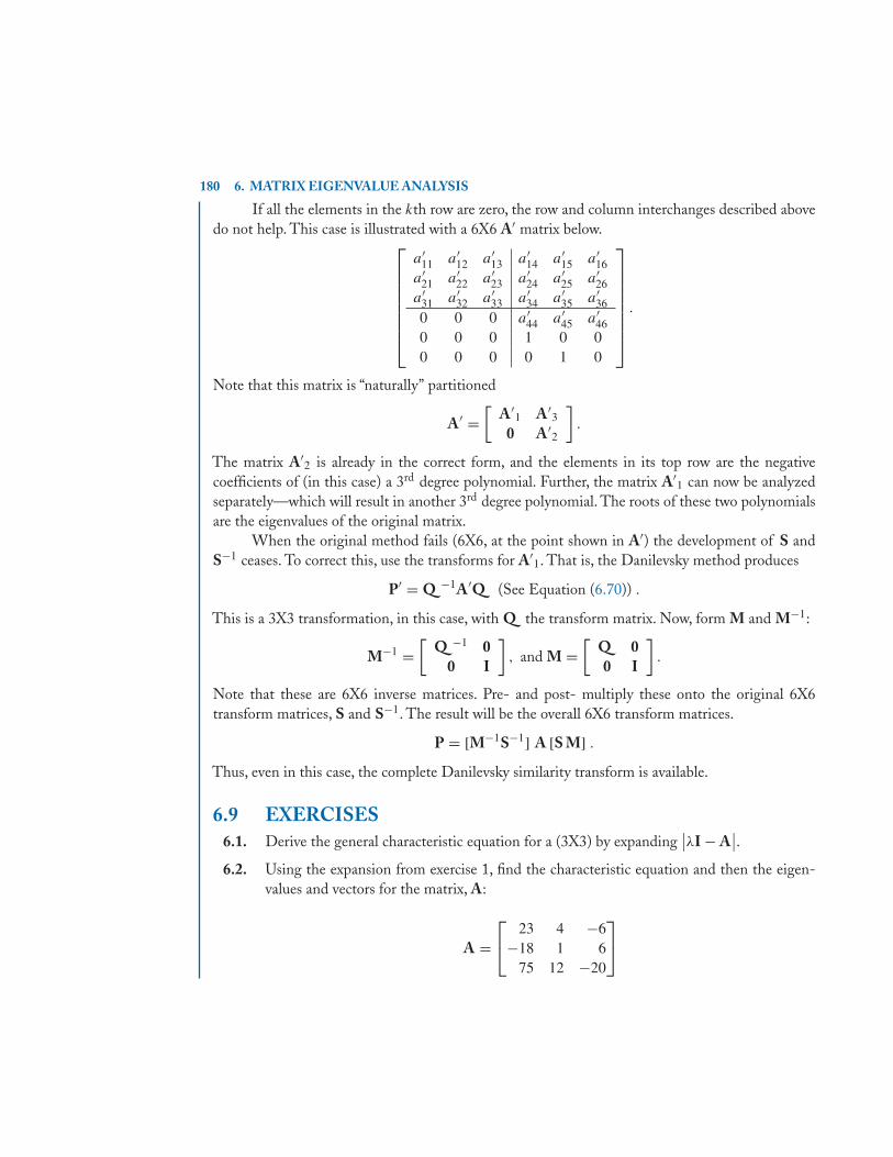
180 6. MATRIX EIGENVALUE ANALYSIS
If all the elements in the kth row are zero, the row and column interchanges described abovedo not help. This case is illustrated with a 6X6 A′ matrix below.⎡
⎢⎢⎢⎢⎢⎢⎢⎣
a′11 a′
12 a′13 a′
14 a′15 a′
16a′
21 a′22 a′
23 a′24 a′
25 a′26
a′31 a′
32 a′33 a′
34 a′35 a′
360 0 0 a′
44 a′45 a′
460 0 0 1 0 00 0 0 0 1 0
⎤⎥⎥⎥⎥⎥⎥⎥⎦
.
Note that this matrix is “naturally” partitioned
A′ =[
A′1 A′
3
0 A′2
].
The matrix A′2 is already in the correct form, and the elements in its top row are the negative
coefficients of (in this case) a 3rd degree polynomial. Further, the matrix A′1 can now be analyzed
separately—which will result in another 3rd degree polynomial. The roots of these two polynomialsare the eigenvalues of the original matrix.
When the original method fails (6X6, at the point shown in A′) the development of S andS−1 ceases. To correct this, use the transforms for A′
1. That is, the Danilevsky method produces
P′ = Q −1A′Q (See Equation (6.70)) .
This is a 3X3 transformation, in this case, with Q the transform matrix. Now, form M and M−1:
M−1 =[
Q −1 00 I
], and M =
[Q 00 I
].
Note that these are 6X6 inverse matrices. Pre- and post- multiply these onto the original 6X6transform matrices, S and S−1. The result will be the overall 6X6 transform matrices.
P = [M−1S−1] A [S M] .
Thus, even in this case, the complete Danilevsky similarity transform is available.
6.9 EXERCISES6.1. Derive the general characteristic equation for a (3X3) by expanding
∣∣λI − A∣∣.
6.2. Using the expansion from exercise 1, find the characteristic equation and then the eigen-values and vectors for the matrix, A:
A =⎡⎣ 23 4 −6
−18 1 675 12 −20
⎤⎦
6.9. EXERCISES 181
6.3. Using the eigenvalue data from Problem 2, find the λk{vk}[uk] matrices (for k =1, 2, 3) andfind the sum of these three matrices.
6.4. (a) Using the same data, find the matrix B = λ1{v1}[u1] + λ2{v2}[u2] and find its charac-teristic equation.
(b) Show that the eigenvectors of B are the same as those for A.
(c) Given B =⎡⎣ 9 −6 −4
−12 3 424 −18 −11
⎤⎦, and the A matrix from Problem 2, find BA and
AB. Explain.
6.5. For the matrix A = 12
[5 −3
−3 5
], find
√A.
6.6. For the matrix A =[ −0.7 2
−0.6 1.5
], find sin(A).
6.7. (a) Given Ax = λx + c, define the conditions under which a solution exists.
(b) Solve the equation assuming the necessary conditions.
(c) If the (2X2) A matrix is that from Problem 5, and the c vector is c = {1, – 1} solve theset in terms of the parameter λ. Does a solution exist when λ = 1?
6.8. In the polynomial6∏
j=1(x − xj ) = x6 + c1x
5 + · · · + cn find c2 and c3. Describe the for-
mation of each of the coefficients.
6.9. Given A =⎡⎣ 6 −3 0
−3 6 −30 −3 4
⎤⎦
(a) Use Danilevsky’s method to find the coefficients of its characteristic polynomial.
(b) Use matrix iteration (Section 6.7.2) to find the largest eigenvalue.
(c) “Divide-out” the root from (b) and solve the quadratic for the remaining eigenvaluesof A.


183
C H A P T E R 7
Matrix Analysis of VibratingSystems
7.1 INTRODUCTIONThe eigenvalue problem, the details of which were discussed in the previous chapter, has applicationin many important areas in engineering. Certainly one of the most interesting is in the study of(linearized) vibrating systems.1 These systems are a perfect and direct example of the CharacteristicValue problem. We will begin there, and add the non-homogeneous set as well:{
Ax − λx = 0Ax − λx = c
(7.1)
Given that A is “diagonalizable” (we omit the defective matrix case from discussion), there exist n
values of λ (“eigenvalues”) for which the homogeneous set has a solution. For each of these values theassociated solutions are the “eigenvectors,” u (row) and v (column). These two sets of solutions areorthogonal to one another: ui•vj = 0 (i �= j). In the event that A is symmetric, the u set is simplythe transpose of the v. In either event, the sets are normalized such that ui•vi = 1.
For the non-homogeneous equation we assume a solution of the form x = Vy. Then:⎧⎪⎪⎨⎪⎪⎩
AVy − λVy = c ; Premultiply by U :UAVy − λy = Uc ; (
UAV = �) :
(� − λI)y = Ucy = (� − λI)−1 Uc
(7.2)
therefore x = Vy = V(� − λI)−1Uc . (7.3)
Apparently, the inverse of (A −λI) is V(� − λI)−1U. Of course this inverse does not exist when λ
is equal to one of the eigenvalues, λi . This fact is the more clear when the inverse is written as:
(� − λI)−1 =[δij • 1
(λj − λ)
]
a diagonal matrix (note the Kronecker delta, δij ). Then, in general the non-homogeneous set hasno solution when λ equals one of the eigenvalues. If, however, the vector, c, is orthogonal to ui ,then the solution (7.3) holds: we maintain the orthogonality while allowing λ to approach λi . In the1It is assumed that the reader is familiar with the differential equations which govern the motion of linear vibrating systems.
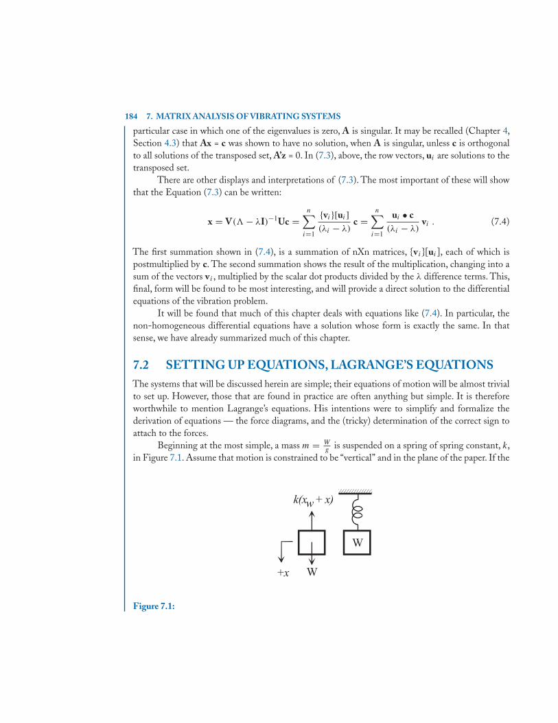
184 7. MATRIX ANALYSIS OF VIBRATING SYSTEMS
particular case in which one of the eigenvalues is zero, A is singular. It may be recalled (Chapter 4,Section 4.3) that Ax = c was shown to have no solution, when A is singular, unless c is orthogonalto all solutions of the transposed set, A’z = 0. In (7.3), above, the row vectors, ui are solutions to thetransposed set.
There are other displays and interpretations of (7.3). The most important of these will showthat the Equation (7.3) can be written:
x = V(� − λI)−1Uc =n∑
i=1
{vi}[ui](λi − λ)
c =n∑
i=1
ui • c(λi − λ)
vi . (7.4)
The first summation shown in (7.4), is a summation of nXn matrices, {vi}[ui], each of which ispostmultiplied by c. The second summation shows the result of the multiplication, changing into asum of the vectors vi , multiplied by the scalar dot products divided by the λ difference terms. This,final, form will be found to be most interesting, and will provide a direct solution to the differentialequations of the vibration problem.
It will be found that much of this chapter deals with equations like (7.4). In particular, thenon-homogeneous differential equations have a solution whose form is exactly the same. In thatsense, we have already summarized much of this chapter.
7.2 SETTING UP EQUATIONS, LAGRANGE’S EQUATIONSThe systems that will be discussed herein are simple; their equations of motion will be almost trivialto set up. However, those that are found in practice are often anything but simple. It is thereforeworthwhile to mention Lagrange’s equations. His intentions were to simplify and formalize thederivation of equations — the force diagrams, and the (tricky) determination of the correct sign toattach to the forces.
Beginning at the most simple, a mass m = Wg
is suspended on a spring of spring constant, k,in Figure 7.1. Assume that motion is constrained to be “vertical” and in the plane of the paper. If the
Figure 7.1:
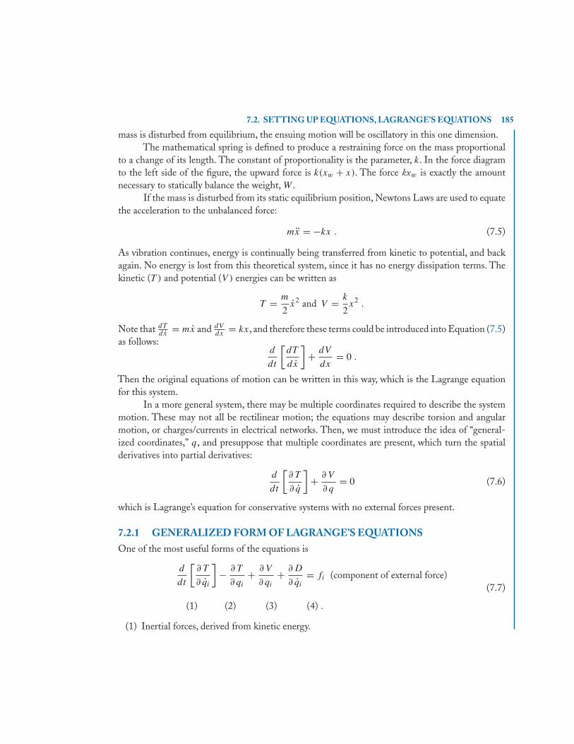
7.2. SETTING UP EQUATIONS, LAGRANGE’S EQUATIONS 185
mass is disturbed from equilibrium, the ensuing motion will be oscillatory in this one dimension.The mathematical spring is defined to produce a restraining force on the mass proportional
to a change of its length. The constant of proportionality is the parameter, k. In the force diagramto the left side of the figure, the upward force is k(xw + x). The force kxw is exactly the amountnecessary to statically balance the weight, W .
If the mass is disturbed from its static equilibrium position, Newtons Laws are used to equatethe acceleration to the unbalanced force:
mx = −kx . (7.5)
As vibration continues, energy is continually being transferred from kinetic to potential, and backagain. No energy is lost from this theoretical system, since it has no energy dissipation terms. Thekinetic (T ) and potential (V ) energies can be written as
T = m
2x2 and V = k
2x2 .
Note that dTdx
= mx and dVdx
= kx, and therefore these terms could be introduced into Equation (7.5)as follows:
d
dt
[dT
dx
]+ dV
dx= 0 .
Then the original equations of motion can be written in this way, which is the Lagrange equationfor this system.
In a more general system, there may be multiple coordinates required to describe the systemmotion. These may not all be rectilinear motion; the equations may describe torsion and angularmotion, or charges/currents in electrical networks. Then, we must introduce the idea of “general-ized coordinates,” q, and presuppose that multiple coordinates are present, which turn the spatialderivatives into partial derivatives:
d
dt
[∂ T
∂ q
]+ ∂ V
∂ q= 0 (7.6)
which is Lagrange’s equation for conservative systems with no external forces present.
7.2.1 GENERALIZED FORM OF LAGRANGE’S EQUATIONSOne of the most useful forms of the equations is
d
dt
[∂ T
∂ qi
]− ∂ T
∂ qi
+ ∂ V
∂ qi
+ ∂ D
∂ qi
= fi (component of external force)
(1) (2) (3) (4) .
(7.7)
(1) Inertial forces, derived from kinetic energy.
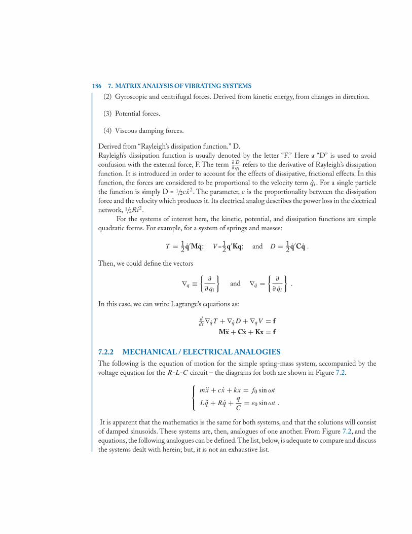
186 7. MATRIX ANALYSIS OF VIBRATING SYSTEMS
(2) Gyroscopic and centrifugal forces. Derived from kinetic energy, from changes in direction.
(3) Potential forces.
(4) Viscous damping forces.
Derived from “Rayleigh’s dissipation function.” D.Rayleigh’s dissipation function is usually denoted by the letter “F.” Here a “D” is used to avoidconfusion with the external force, F. The term ∂ D
∂ qirefers to the derivative of Rayleigh’s dissipation
function. It is introduced in order to account for the effects of dissipative, frictional effects. In thisfunction, the forces are considered to be proportional to the velocity term qi . For a single particlethe function is simply D = 1/2cx
2. The parameter, c is the proportionality between the dissipationforce and the velocity which produces it. Its electrical analog describes the power loss in the electricalnetwork, 1/2Ri2.
For the systems of interest here, the kinetic, potential, and dissipation functions are simplequadratic forms. For example, for a system of springs and masses:
T = 12 q′Mq; V =1
2 q′Kq; and D = 12 q′Cq .
Then, we could define the vectors
∇q ≡{
∂
∂ qi
}and ∇q =
{∂
∂ qi
}.
In this case, we can write Lagrange’s equations as:
ddt
∇qT + ∇qD + ∇qV = f
Mx + Cx + Kx = f
7.2.2 MECHANICAL / ELECTRICAL ANALOGIESThe following is the equation of motion for the simple spring-mass system, accompanied by thevoltage equation for the R-L-C circuit – the diagrams for both are shown in Figure 7.2.
⎧⎨⎩
mx + cx + kx = f0 sin ωt
Lq + Rq + q
C= e0 sin ωt .
It is apparent that the mathematics is the same for both systems, and that the solutions will consistof damped sinusoids. These systems are, then, analogues of one another. From Figure 7.2, and theequations, the following analogues can be defined.The list, below, is adequate to compare and discussthe systems dealt with herein; but, it is not an exhaustive list.
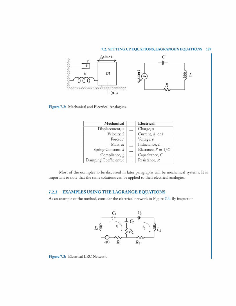
7.2. SETTING UP EQUATIONS, LAGRANGE’S EQUATIONS 187
Figure 7.2: Mechanical and Electrical Analogues.
Mechanical ElectricalDisplacement, x Charge, q
Velocity, x Current, q or i
Force, f Voltage, eMass, m Inductance, L
Spring Constant, k Elastance, S = 1/C
Compliance, 1k
Capacitance, CDamping Coefficient, c Resistance, R
Most of the examples to be discussed in later paragraphs will be mechanical systems. It isimportant to note that the same solutions can be applied to their electrical analogies.
7.2.3 EXAMPLES USING THE LAGRANGE EQUATIONSAs an example of the method, consider the electrical network in Figure 7.3. By inspection
Figure 7.3: Electrical LRC Network.
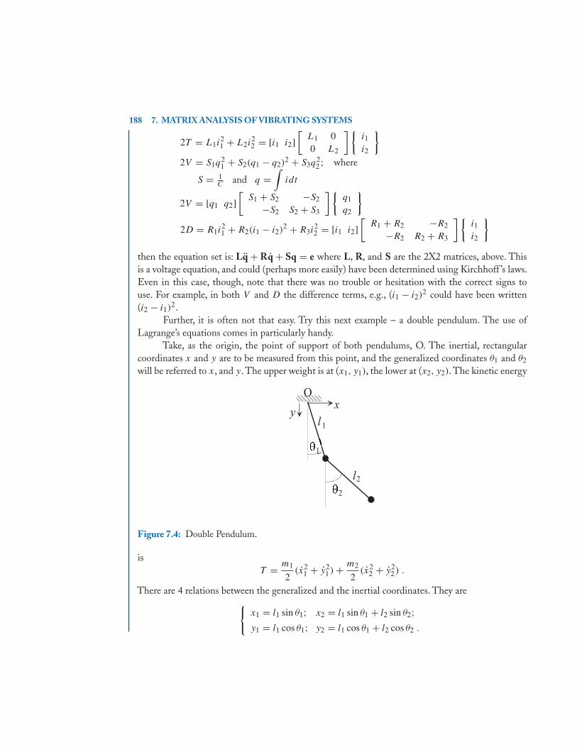
188 7. MATRIX ANALYSIS OF VIBRATING SYSTEMS
2T = L1i21 + L2i
22 = [i1 i2]
[L1 00 L2
]{i1
i2
}2V = S1q
21 + S2(q1 − q2)
2 + S3q22 ; where
S = 1C
and q =∫
idt
2V = [q1 q2][
S1 + S2 −S2
−S2 S2 + S3
]{q1
q2
}
2D = R1i21 + R2(i1 − i2)
2 + R3i22 = [i1 i2]
[R1 + R2 −R2
−R2 R2 + R3
]{i1
i2
}
then the equation set is: Lq + Rq + Sq = e where L, R, and S are the 2X2 matrices, above. Thisis a voltage equation, and could (perhaps more easily) have been determined using Kirchhoff ’s laws.Even in this case, though, note that there was no trouble or hesitation with the correct signs touse. For example, in both V and D the difference terms, e.g., (i1 − i2)
2 could have been written(i2 − i1)
2.Further, it is often not that easy. Try this next example – a double pendulum. The use of
Lagrange’s equations comes in particularly handy.Take, as the origin, the point of support of both pendulums, O. The inertial, rectangular
coordinates x and y are to be measured from this point, and the generalized coordinates θ1 and θ2
will be referred to x, and y. The upper weight is at (x1, y1), the lower at (x2, y2). The kinetic energy
Figure 7.4: Double Pendulum.
isT = m1
2(x2
1 + y21) + m2
2(x2
2 + y22) .
There are 4 relations between the generalized and the inertial coordinates. They are{x1 = l1 sin θ1; x2 = l1 sin θ1 + l2 sin θ2;y1 = l1 cos θ1; y2 = l1 cos θ1 + l2 cos θ2 .
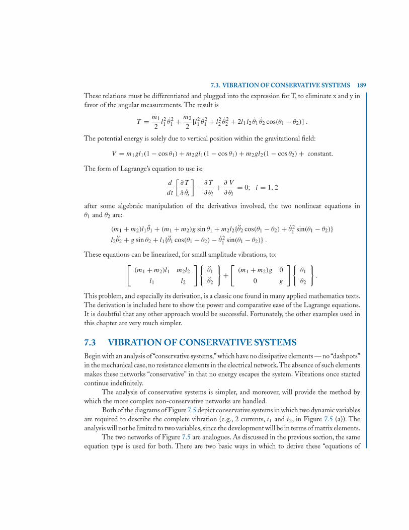
7.3. VIBRATION OF CONSERVATIVE SYSTEMS 189
These relations must be differentiated and plugged into the expression for T, to eliminate x and y infavor of the angular measurements. The result is
T = m1
2l21 θ2
1 + m2
2[l2
1 θ21 + l2
2 θ22 + 2l1 l2 θ1 θ2 cos(θ1 − θ2)] .
The potential energy is solely due to vertical position within the gravitational field:
V = m1gl1(1 − cos θ1) + m2gl1(1 − cos θ1) + m2gl2(1 − cos θ2) + constant.
The form of Lagrange’s equation to use is:
d
dt
[∂ T
∂ θi
]− ∂ T
∂ θi
+ ∂ V
∂ θi
= 0; i = 1, 2
after some algebraic manipulation of the derivatives involved, the two nonlinear equations inθ1 and θ2 are:
(m1 + m2)l1θ1 + (m1 + m2)g sin θ1 + m2l2{θ2 cos(θ1 − θ2) + θ21 sin(θ1 − θ2)}
l2θ2 + g sin θ2 + l1{θ1 cos(θ1 − θ2) − θ21 sin(θ1 − θ2)} .
These equations can be linearized, for small amplitude vibrations, to:[(m1 + m2)l1 m2l2
l1 l2
]{θ1
θ2
}+[
(m1 + m2)g 0
0 g
]{θ1
θ2
}.
This problem, and especially its derivation, is a classic one found in many applied mathematics texts.The derivation is included here to show the power and comparative ease of the Lagrange equations.It is doubtful that any other approach would be successful. Fortunately, the other examples used inthis chapter are very much simpler.
7.3 VIBRATION OF CONSERVATIVE SYSTEMSBegin with an analysis of “conservative systems,” which have no dissipative elements — no “dashpots”in the mechanical case, no resistance elements in the electrical network.The absence of such elementsmakes these networks “conservative” in that no energy escapes the system. Vibrations once startedcontinue indefinitely.
The analysis of conservative systems is simpler, and moreover, will provide the method bywhich the more complex non-conservative networks are handled.
Both of the diagrams of Figure 7.5 depict conservative systems in which two dynamic variablesare required to describe the complete vibration (e.g., 2 currents, i1 and i2, in Figure 7.5 (a)). Theanalysis will not be limited to two variables, since the development will be in terms of matrix elements.
The two networks of Figure 7.5 are analogues. As discussed in the previous section, the sameequation type is used for both. There are two basic ways in which to derive these “equations of
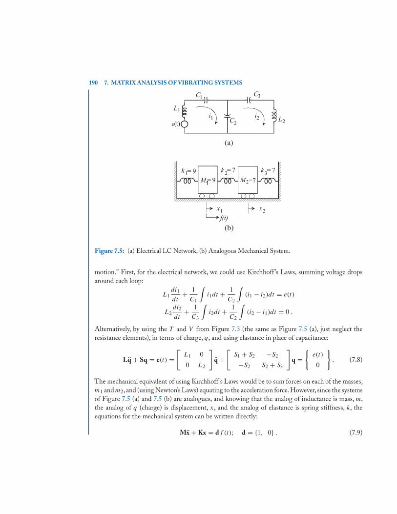
190 7. MATRIX ANALYSIS OF VIBRATING SYSTEMS
Figure 7.5: (a) Electrical LC Network, (b) Analogous Mechanical System.
motion.” First, for the electrical network, we could use Kirchhoff ’s Laws, summing voltage dropsaround each loop:
L1di1
dt+ 1
C1
∫i1dt + 1
C2
∫(i1 − i2)dt = e(t)
L2di2
dt+ 1
C3
∫i2dt + 1
C2
∫(i2 − i1)dt = 0 .
Alternatively, by using the T and V from Figure 7.3 (the same as Figure 7.5 (a), just neglect theresistance elements), in terms of charge, q, and using elastance in place of capacitance:
Lq + Sq = e(t) =[
L1 0
0 L2
]q +
[S1 + S2 −S2
−S2 S2 + S3
]q =
{e(t)
0
}. (7.8)
The mechanical equivalent of using Kirchhoff ’s Laws would be to sum forces on each of the masses,m1 and m2, and (using Newton’s Laws) equating to the acceleration force. However, since the systemsof Figure 7.5 (a) and 7.5 (b) are analogues, and knowing that the analog of inductance is mass, m,the analog of q (charge) is displacement, x, and the analog of elastance is spring stiffness, k, theequations for the mechanical system can be written directly:
Mx + Kx = df (t); d = {1, 0} . (7.9)
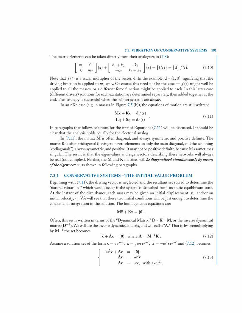
7.3. VIBRATION OF CONSERVATIVE SYSTEMS 191
The matrix elements can be taken directly from their analogues in (7.8):[m1 00 m2
]{x} +
[k1 + k2 −k2
−k2 k2 + k3
]{x} = {
f (t)} = {
d}f (t). (7.10)
Note that f (t) is a scalar multiplier of the vector, d. In the example, d = {1, 0}, signifying that thedriving function is applied to m1 only. Of course this need not be the case — f (t) might well beapplied to all the masses, or a different force function might be applied to each. In this latter case(different drivers) solutions for each excitation are determined separately, then added together at theend. This strategy is successful when the subject systems are linear.
In an nXn case (e.g., n masses in Figure 7.5 (b)), the equations of motion are still written:
Mx + Kx = df (t)
Lq + Sq = de(t). (7.11)
In paragraphs that follow, solutions for the first of Equations (7.11) will be discussed. It should beclear that the analysis holds equally for the electrical analog.
In (7.11), the matrix M is often diagonal, and always symmetric and positive definite. Thematrix K is often tridiagonal (having non zero elements on only the main diagonal, and the adjoining“codiagonals”), always symmetric, and positive. It may not be positive definite,because it is sometimessingular. The result is that the eigenvalues and eigenvectors describing these networks will alwaysbe real (not complex). Further, the M and K matrices will be diagonalized simultaneously by meansof the eigenvectors, as shown in following paragraphs.
7.3.1 CONSERVATIVE SYSTEMS – THE INITIAL VALUE PROBLEMBeginning with (7.11), the driving vector is neglected and the resultant set solved to determine the“natural vibrations” which would occur if the system is disturbed from its static equilibrium state.At the instant of the disturbance, each mass may be given an initial displacement, x0, and/or aninitial velocity, x0. We will see that these two initial conditions will be just enough to determine theconstants of integration in the solution. The homogeneous equations are:
Mx + Kx = {0} .
Often, this set is written in terms of the “Dynamical Matrix,” D = K−1M, or the inverse dynamicalmatrix (D−1).We will use the inverse dynamical matrix, and will call it “A.”That is,by premultiplyingby M−1 the set becomes
x + Ax = {0}, where A = M−1K . (7.12)
Assume a solution set of the form x = vejωt , x = jωvejωt , x = −ω2vejωt and (7.12) becomes:⎧⎪⎨⎪⎩
−ω2v + Av = {0}Av = ω2vAv = λv, with λ=ω2 .
(7.13)
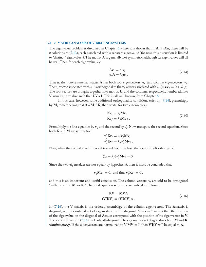
192 7. MATRIX ANALYSIS OF VIBRATING SYSTEMS
The eigenvalue problem is discussed in Chapter 6 where it is shown that if A is nXn, there will ben solutions to (7.13), each associated with a separate eigenvalue (for now, this discussion is limitedto “distinct” eigenvalues). The matrix A is generally not symmetric, although its eigenvalues will allbe real. Then for each eigenvalue, λi :
Avi = λivi
uiA = λiui .(7.14)
That is, the non-symmetric matrix A has both row eigenvectors, ui , and column eigenvectors, vi .The ui vector associated with λj is orthogonal to the vi vector associated with λi (ui•vj = 0, i �= j).The row vectors are brought together into matrix, U, and the columns, respectively, numbered, intoV, usually normalize such that UV = I. This is all well known, from Chapter 6.
In this case, however, some additional orthogonality conditions exist. In (7.14), premultiplyby M, remembering that A = M−1K, then write, for two eigenvectors:
Kvi = λiMvi
Kvj = λj Mvj .(7.15)
Premultiply the first equation by v′j and the second by v′
i . Now, transpose the second equation. Sinceboth K and M are symmetric:
v ′j Kvi = λiv ′
j Mvi
v ′j Kvi = λj v ′
j Mvi .
Now, when the second equation is subtracted from the first, the identical left sides cancel
(λi − λj )v ′j Mvi = 0 .
Since the two eigenvalues are not equal (by hypothesis), then it must be concluded that
v ′j Mvi = 0, and thus v ′
j Kvi = 0 ,
and this is an important and useful conclusion. The column vectors, v, are said to be orthogonal“with respect to M, or K.” The total equation set can be assembled as follows:
KV = MV�
(V ′KV) = (V ′MV)� .(7.16)
In (7.16), the V matrix is the ordered assemblage of the column eigenvectors. The ���matrix isdiagonal, with its ordered set of eigenvalues on the diagonal. “Ordered” means that the positionof the eigenvalue on the diagonal of ���must correspond with the position of its eigenvector in V.The second Equation (7.16) is clearly all-diagonal. The eigenvector set diagonalizes both M and K,simultaneously. If the eigenvectors are normalized to V′MV = I, then V′KV will be equal to ���.
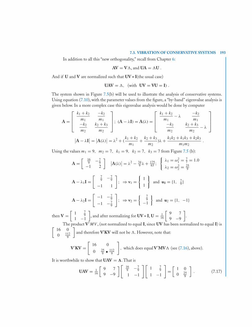
7.3. VIBRATION OF CONSERVATIVE SYSTEMS 193
In addition to all this “new orthogonality,” recall from Chapter 6:
AV = V�, and UA = �U .
And if U and V are normalized such that UV = I(the usual case)
UAV = �, (with UV = VU = I) .
The system shown in Figure 7.5(b) will be used to illustrate the analysis of conservative systems.Using equation (7.10), with the parameter values from the figure, a “by-hand” eigenvalue analysis isgiven below. In a more complex case this eigenvalue analysis would be done by computer
A =
⎡⎢⎢⎣
k1 + k2
m1
−k2
m1−k2
m2
k2 + k3
m2
⎤⎥⎥⎦ ; (A − λI) = A(λ) =
⎡⎢⎢⎣
k1 + k2
m1− λ
−k2
m1−k2
m2
k2 + k3
m2− λ
⎤⎥⎥⎦
∣∣A − λI∣∣ = ∣∣A(λ)
∣∣ = λ2 + (k1 + k2
m1+ k2 + k3
m2)λ + k1k2 + k1k3 + k2k3
m1m2.
Using the values m1 = 9, m2 = 7, k1 = 9, k2 = 7, k3 = 7 from Figure 7.5 (b):
A =[ 16
9 − 79
−1 2
] ∣∣A(λ)∣∣ = λ2 − 34
9 λ + 17563 ;
{λ1 = ω2
1 = 77 = 1.0
λ2 = ω22 = 25
9
A − λ1I =[ 7
9 − 79
−1 1
]; ⇒ v1 =
{1
1
}and u1 = {1, 7
9 }
A − λ2I =[
−1 − 79
−1 − 79
]; ⇒ v2 =
{ 79
−1
}and u2 = {1, −1}
then V =[
1 79
1 −1
], and after normalizing for UV = I, U = 1
16
[9 79 −9
].
The product V ′MV , (not normalized to equal I, since UV has been normalized to equal I) is[16 00 112
9
]and therefore V′KV will not be �. However, note that:
V ′KV =[
16 0
0 259 • 112
9
], which does equal V ′MV� (see (7.16), above).
It is worthwhile to show that UAV = �. That is
UAV = 116
[9 79 −9
][ 169 − 7
9
1 −1
][1 7
9
1 −1
]=[
1 00 25
9
]. (7.17)
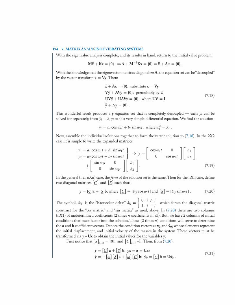
194 7. MATRIX ANALYSIS OF VIBRATING SYSTEMS
With the eigenvalue analysis complete, and its results in hand, return to the initial value problem:
Mx + Kx = {0} ⇒ x + M−1Kx = {0} = x + Ax = {0} .
With the knowledge that the eigenvector matrices diagonalize A, the equation set can be “decoupled”by the vector transform x = Vy. Then:
x + Ax = {0}; substitute x = Vy
Vy + AVy = {0}; premultiply by U
UVy + UAVy = {0}; where UV = I
y + �y = {0} .
(7.18)
This wonderful result produces a y equation set that is completely decoupled — each yi can besolved for separately, from yi + λiyi = 0, a very simple differential equation. We find the solution
yi = ai cos ωit + bi sin ωit; where ω2i = λi .
Now, assemble the individual solutions together to form the vector solution to (7.18), In the 2X2case, it is simple to write the expanded matrices:
y1 = a1 cos ω1t + b1 sin ω1t
y2 = a2 cos ω2t + b2 sin ω2t
}⇒ y =
[cos ω1t 0
0 cos ω2t
][a1
a2
]
+[
sin ω1t 0
0 sin ω2t
][b1
b2
]. (7.19)
In the general (i.e., nXn) case, the form of the solution set is the same. Then for the nXn case, definetwo diagonal matrices
[C]
and[S]
such that:
y = [C]a + [S]b; where[C] ≡ [δij cos ωit] and
[S] ≡ [δij sin ωit] . (7.20)
The symbol, δij , is the “Kronecker delta:” δij ={
0, i �= j
1, i = jwhich forces the diagonal matrix
construct for the “cos matrix” and “sin matrix” as used, above. In (7.20) there are two columns(nX1) of undetermined coefficients (2 times n coefficients in all). But, we have 2 columns of initialconditions that must factor into the solution. These (2 times n) conditions will serve to determinethe a and b coefficient vectors. Denote the condition vectors as x0 and x0, whose elements representthe initial displacement, and initial velocity of the masses in the system. These vectors must betransformed via y = Ux to obtain the initial values for the variables y.
First notice that[S]t=0 = [0], and
[C]t=0 =I. Then, from (7.20):
y = [C]
a + [S]
b; y0 = a = Ux0
y = − [ω] [
S]
a + [ω] [
C]
b; y0 = [ω]
b = Ux0 .(7.21)
7.3. VIBRATION OF CONSERVATIVE SYSTEMS 195
In the second of (7.21) the matrix[ω]
is diagonal = [δijωi]. Then a = Ux0 and b = [ω]−1 Ux0
y = [C]
Ux0 + [S] [
ω]−1 Ux0 (7.22)
and since x =Vy, we premultiply (7.22) by V to return to the x variables.
x = V[C]
Ux0 + V[S] [
ω]−1 Ux0 . (7.23)
At first, (7.23) appears to be very formidable, and not easily programmed.[C]
and[S]
are func-tions of time. A straightforward expansion would be very messy. Fortunately, there is an excellentinterpretation of (7.23) which not only makes it clearer to “see,” but, is also easily programmed.
7.3.2 INTERPRETATION OF EQUATION (7.23)In the previous chapter there is a discussion of the synthesis of a matrix by its eigenvalues andeigenvectors. Equation (6.14) of that chapter reads:
A =n∑
i=1
λi{vi}[ui] . (Chapter 6, (6.14))
This result occurs through an interpretation of A = V�U. The central idea is that � is a diagonalmatrix. Its j th main diagonal element, i.e., λj , multiplies the j th column of V (or form the product�U first, in which case, the j th eigenvalue will be a multiplier on the j th row vector in U).
The same logic is used here concerning the term V[C]
Ux0 in (7.23). In this case,[C]
is thediagonal matrix. Its j th term is cos ωj t and it multiplies the jth column of V. Now, view the V
[C]
matrix as partitioned by columns:
V[C] =
⎡⎣⎧⎨⎩
· · ·v1 cos ω1t
· · ·
⎫⎬⎭⎧⎨⎩
· · ·v2 cos ω2t
· · ·
⎫⎬⎭ · · ·
⎧⎨⎩
· · ·vn cos ωnt
· · ·
⎫⎬⎭⎤⎦
and the U matrix partitioned by rows, and the product is written:
V[C]
U = v1u1 cos ω1t + v2u2 cos ω2t + · · · + vnun cos ωnt =n∑
i=1
viui cos ωit
a summation of nXn’s, each multiplied by the corresponding diagonal element of the center matrix.This is the same (desired) result as before (Chapter 6; (6.14)) – with the λi values replaced by thecos ωit terms. Now, the term V
[C]U does not look at all formidable, since the time varying terms
appear as multipliers on an entire matrix entity.And, it gets better. Note that V
[C]U involves summing n nXn’s. But, when the x0 vector is
post multiplied, it actually simplifies the sum – it is easier to operate with vectors than matrices. Since
196 7. MATRIX ANALYSIS OF VIBRATING SYSTEMS
the ui terms are rows, they are “available” to dot into the x0 vector. Then;
V[C]
Ux0 =n∑
i=1
vi (ui • x0) cos ωit . (7.24)
And the term is now composed of just n eigenvectors, weighted as shown in (7.24). This is easilyvisualized, and easily coded. The time dependent (cos) terms are straightforward scalar multipliers,as are the dot product ui • x0 terms.
Returning to (7.23), its second term can now be written out by inspection. Note that theproduct
[S] [
ω]−1 is still just a diagonal, sandwiched between V and U. The inverse
[ω]−1 is just[
δij1ωi
].
V[S] [
ω]−1 Ux0 =
n∑i=1
vi (ui • x0)1
ωi
sin ωit (7.25)
and now, putting (7.14) and (7.25) together:
x =n∑
i=1
vi (ui • x0) cos ωit +n∑
i=1
vi (ui • x0)1
ωi
sin ωit. (7.26)
This is a general result, the initial value problem solution applicable to nXn systems (networks).Notice that the eigenvalue analysis is “sum and substance” of the solution. Except for the giveninitial conditions, all terms are from that analysis (it is required that the eigenvalue analysis producesboth sets of eigenvectors, normalized such that UV = I.)
In the particular 2X2 example from Figure 7.5 (b), with the initial conditions x0 {1, 0} andx0 = {0, 1}, we find
u1 • x0 = 916 × 1 + 7
16 × 0 = 916
u2 • x0 = 916 × 1 + (− 9
16 ) × 0 = 916
u1 • x0 = 916 × 0 + 7
16 × 1 = 716
u2 • x0 = 916 × 0 + (− 9
16 ) × 1 = − 916 .
Plugging these values into (7.26):
x = 9
16
{11
}cos 1t + 9
16
{79
−1
}cos 5
3 t + 716
{1
1
}sin 1t− 9
16 • 35
{79
−1
}sin 5
3 t. (7.27)
From the display in (7.27), it is clear how the v vectors sum to form the total solution. These veigenvectors are called the “normal modes” of the vibration.The absolute amplitudes of the vibrationare of course strongly affected by the initial conditions. But, at each of the frequencies, the ratios of the
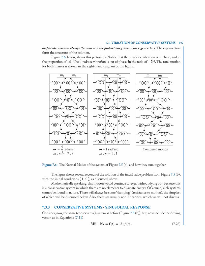
7.3. VIBRATION OF CONSERVATIVE SYSTEMS 197
amplitudes remains always the same – in the proportions given in the eigenvectors. The eigenvectorsform the structure of the solution.
Figure 7.6, below, shows this pictorially. Notice that the 1 rad/sec vibration is in phase, and inthe proportion of 1:1. The 5
3 rad/sec vibration is out of phase, in the ratio of −7:9. The total motionfor both masses is shown in the right-hand diagram of the figure.
Figure 7.6: The Normal Modes of the system of Figure 7.5 (b), and how they sum together.
The figure shows several seconds of the solution of the initial value problem from Figure 7.5 (b),with the initial conditions { 1 0 }, as discussed, above.
Mathematically speaking, this motion would continue forever, without dying out, because thisis a conservative system in which there are no elements to dissipate energy. Of course, such systemscannot be found in nature.There will always be some “damping” (resistance to motion), the simplestof which will be discussed below. Also, there are usually non-linearities, which we will not discuss.
7.3.3 CONSERVATIVE SYSTEMS - SINUSOIDAL RESPONSEConsider, now, the same (conservative) system as before (Figure 7.5 (b)), but, now include the drivingvector, as in Equations (7.11)
Mx + Kx = f (t) = {d}f (t) . (7.28)
198 7. MATRIX ANALYSIS OF VIBRATING SYSTEMS
We will assume the function f (t) = cos ωt . Premultiply (7.28) by M−1 (M is nonsingular) andagain make the vector transform x = Vy
x + Ax = M−1d cos t
y + �y = UM−1d cos ωt
We assume the particular solution y = Y cos ωt; y = − [ω]
Y sin ωt; y = − [ω2]
Y cos ωt :
− [ω2]
Y + �Y = UM−1d; [ω2] = [
ω] [
ω]
Y = [δij (λi − ω2)
]−1 UM−1d
where[δij (ω
2i − ω2)
]is a diagonal matrix; and note that λi = ω2
i .The homogeneous solution is already known to be
[C]
a + [S]
b. Then:
y = [C]
a + [S]
b +[δij (ω
2i − ω2)
]−1UM−1d cos ωt . (7.29)
Assuming that the system is initially at rest x0 = y0 = x0 = y0 = 0, it is a simple matter to solve fora (b is clearly 0), and the solution, x = Vy, becomes
x =n∑
i=1
vi (ui • M−1d)cos ωt
ω2i − ω2
−n∑
i=1
vi (ui • M−1d)cos ωit
ω2i − ω2
. (7.30)
Note that the first term (the summation multiplied by the driving frequency) need not be writtenas a summation. Since the only function of time is already a separate multiplier, this term could be“interpreted-back” into the matrix operations: V
[� − ω2
]−1 UM−1d cos ωt .That is, the single timefunction,cos ωt , (ω without subscript refers to the driving frequency) multiplies all of the eigenvectorsin its summation. In the second summation, each multiplier, cos ωit , multiplies its correspondingvector, vi . Because of this (second) term, the vector summation is required – and it is the same sum asin the previous term. Therefore, the vector form of (7.30) is clearer, and the corresponding programsimpler, written this way. In fact, (7.30) can be written:
x =n∑
i=1
vi (ui • M−1d)cos ωt − cos ωit
ω2i − ω2
. (7.31)
A conservative system should not be driven at a frequency equal, or very close to, one of the natural,“mode frequencies.” Equation (7.30) clearly indicates why, with the difference frequencies in thedenominator. However, note that if the corresponding dot product term ui • M−1d is zero, thenthat eigenvector-term will not appear in the sum. The condition required for this to be true can bedetermined as follows:
It has already been established that V′MV = P is a diagonal matrix.The values of the diagonalelements of P (they’ll all be positive) depend on the normalization. But, the inverse of P is:
P−1 = UM−1U′
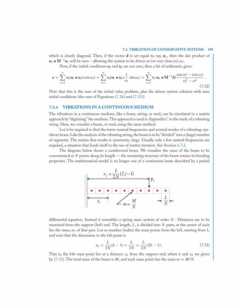
7.3. VIBRATION OF CONSERVATIVE SYSTEMS 199
which is clearly diagonal. Then, if the vector d is set equal to, say, u1, then the dot product ofu2 • M−1u1 will be zero – allowing the system to be driven at (or very close to) ω2.
Now, if the initial conditions x0 and x0 are not zero, then a bit of arithmetic gives:
x =n∑
i=1
vi(ui • x0) cos ωit +n∑
i=1
vi(ui • x0)1
ωi
sin ωit +n∑
i=1
vi (ui • M−1d)cos ωt − cos ωit
ω2i − ω2
.
(7.32)Note that this is the sum of the initial value problem, plus the driven system solution with zeroinitial conditions (the sum of Equations (7.26) and (7.31)).
7.3.4 VIBRATIONS IN A CONTINUOUS MEDIUMThe vibrations in a continuous medium, like a beam, string, or reed, can be simulated in a matrixapproach by “digitizing” the medium.This approach is used in Appendix C in the study of a vibratingstring. Here, we consider a beam, or reed, using the same method.
Let it be required to find the lower natural frequencies and normal modes of a vibrating can-tilever beam.Like the analysis of the vibrating string, the beam is to be “divided” into a (large) numberof segments. The matrix that results is symmetric, large. Usually only a few natural frequencies arerequired, a situation that lends itself to the use of matrix iteration. See Section 6.7.2.
The diagram below shows a cantilevered beam. We visualize the mass of the beam to beconcentrated at N points along its length — the remaining structure of the beam retains its bendingproperties. The mathematical model is no longer one of a continuous beam described by a partial
differential equation. Instead it resembles a spring mass system of order N . Distances are to bemeasured from the support (left) end. The length, L, is divided into N parts, at the center of eachlies the mass, m, of that part. Let us number (index) the mass points from the left, starting from 1,and note that the dimension to the kth point is
xk = L
2N(k − 1) + L
2N= L
2N(2k − 1) . (7.33)
That is, the kth mass point lies at a distance xk from the support end, where k and xk are givenby (7.33). The total mass of the beam is M , and each mass point has the mass m = M/N .
200 7. MATRIX ANALYSIS OF VIBRATING SYSTEMS
From the equations governing the bending of such a beam, the deflection, y(x), at a point x,caused by a load, p, applied at a point s, is
y(x) = px2
EI
( s
2− x
6
); x < s
y(x) = ps2
EI
(x
2− s
6
); x > s
where E is Young’s Modulus, the ratio of stress, psi, to strain, in./in.; and I is the second momentof the beam’s cross sectional area, in.4. Note that the two equations are reciprocal in x and s.
The deflection at x, caused by the load at s, is the same as a deflection at s caused by the loadat x. This “reciprocity” assures that the matrix to be defined below, will be symmetric.
Deflections are of interest only at the mass points. In particular, the deflection y(xi) is writtenyi and we denote the positions of the loads, pj ′ , as xj ′ . Then the deflections are
yi = 1
EI
∑j
i′2L2
4N2
(j ′L4N
− i′L12N
)pj ; Note:
(i′, j ′ = 1, 3, 5 · · · (2N − 1)
i′ < j ′)
. (7.34)
The deflection at point i′ is the sum of the elemental deflections caused by all the loads at pointsxj ′ . The term on the right side (a function of i′ and j ′) defines the elements of an N by N matrix�i,j . The matrix equation can then be written
(y) = L3
EI�i,j (p)
�i,j =[
i′2
16N3
(j ′ − i′
3
)]; �j,i = �i,j ; i′ = 2i − 1, j ′ = 2j − 1 .
(7.35)
As explained, the vector y ={yi} is the deflections at the mass points. The vector p consists of theloads at these same points. In the vibrating beam, these are the D’Alembert inertial loads and areseen to be in the negative direction – opposite to the direction of positive deflection:
pj = −myj = −M
Nyj .
Now, Equation (7.35) can be updated:
y = −ML3
EI�y
�i,j = i′2
16N4
(j ′ − i′
3
); �j,i = �i,j .
(7.36)
Assuming solutions of the form y = vcosωt (y = −vω2 cos ωt):
v cos ωt = −ML3
EI�(−vω2 cos ωt)
λv = �v; where λ = EI
ω2ML3.
(7.37)
7.4. NONCONSERVATIVE SYSTEMS. VISCOUS DAMPING 201
The last of Equations (7.37) is the eigenvalue problem, where the elements of � are defined in (7.36).From this point, iteration is used to derive the eigenvalues and eigenvectors as discussed in Chapter 6.Note that the iteration procedure converges to the largest eigenvalue, but to the smallest naturalfrequency — the one of most interest.
This very interesting approach, is also very simple. However, it is approximate by nature, andbecomes more so as the matrix is deflated after each eigenvalue, eigenvector is found.
7.4 NONCONSERVATIVE SYSTEMS. VISCOUS DAMPINGThe introduction of viscous damping terms is a very serious complication. There is no (eigenvector)matrix which simultaneously diagonalizes 3 matrices. Then, the equations:
Lq + Rq + Sq = {d}e(t)Mx + Cx + Kx = {d}f (t)
(7.38)
cannot easily be attacked directly, at least in the same way that conservative systems were. Forexample, if x = veλt is substituted into (7.38), then, for the homogeneous system:[
Mλ2 + Cλ + K]
v = 0
wherein the nXn matrix elements can be written:∥∥∥∥∥∥∥∥m11λ
2 + c11λ + k11 m12λ2 + c12λ + k12 . . . . . . m1nλ
2 + c1nλ + k1n
m21λ2 + c21λ + k21 . . . . . . . . . . . . . . . . . . .
. . . . . . . . . . . . . . . . . . . . . . . .
mn1λ2 + cn1λ + kn1 . . . . . . . . . . . . mnnλ
2 + cnnλ + knn
∥∥∥∥∥∥∥∥This is the “Lambda Matrix” for the system. The characteristic equation can be found by hand-calculating the determinant of the matrix. The order of the polynomial will be 2n, there will be 2n
eigenvalues, and each will be associated with a row and column vector. But, there does not appear tobe a more systematic way to attack the problem — one that uses the power of the computer, and/orone that provides the familiar Ax −λx = 0, characteristic equation.
A systematic approach is available. The central point is to reduce the equation set to first order.This can be done in the general case, where the original equations are order m.The result is a Lambdamatrix of the recognizable type.
First, define the operator p = d
dt, and note that the original set is written:
[A0pn + A1p
n−1 + · · · + An−1p + An]x = f
where n > 1, and the order of Ai is m. Assuming that the matrix A0 is not singular, the set can bereduced to first order, after premultiplying by the inverse of A0:
202 7. MATRIX ANALYSIS OF VIBRATING SYSTEMS
The reduced set is: py = Ay + g where the vectors y and g are given by
y = {x1 . . . xm, px1 . . . pxm, . . . . . . , pn−1x1 . . . pn−1xm}, and
g = {0, 0, . . . , A−10 f} .
The new A matrix in py = Ay + g is nmXnm. It is diagrammed, below. It is partitioned into squarematrices of order m: each 0 represents an mXm null, and Im represents the order m unit matrix:Note that the Im submatrices are not on the main diagonal, but, the first upper codiagonal.
A =
⎡⎢⎢⎢⎢⎣
0 Im 0 · · · 0 00 0 Im · · · 0 0· · · · · · · · ·0 0 0 · · · 0 Im
−an −an−1 · · · −a1
⎤⎥⎥⎥⎥⎦ , an nXn with each element an mXm.
The mXm submatrices are ai = A−10 Ai .
In particular, when the equations are the Lagrangian equations for small vibrations of a linearsystem, in the generalized coordinates, q, then
Mq + Cq + Kq = f , |M| not equal to zero
can be reduced to the 2mX2m set
z − Az = B−1h, where A =[
0 I−M−1K −M−1C
]; and B =
[C MM 0
].
The very same results are achieved by a method attributed to K. A Foss,2 although the developmentwhich follows is slightly different. It is worthwhile to follow from the beginning, because it verycarefully preserves symmetric submatrices.
Considering the second Equation of (7.38), a trivial equation is added:
Mx + Cx + Kx = {d}f (t)
Mx − Mx = 0(7.39)
Now, define h ={
d0
}and z =
{xx
}, and write the set (7.39) as:
[C MM 0
]{xx
}+[
K 00 −M
]{xx
}={
f0
}= h. (7.40)
2“Coordinates Which Uncouple the Equations of Motion of Damped Linear Systems,” submitted to the ASME Applied MechanicsDivision, May, 1957, by K. A Foss, Massachusetts Institute of Technology.
7.4. NONCONSERVATIVE SYSTEMS. VISCOUS DAMPING 203
This can be written:
Bz + Gz = h; where B =[
C MM 0
], and G =
[K 00 −M
]. (7.41)
In (7.41), 0 is the nXn null matrix, and it should be recalled that M, C, and K are symmetric.Therefore, both B and G are symmetric! A good sign, it looks like the conservative case, except thatthe z vector appears in first derivative, rather than second.
The inverse of B is
B−1 =[
0 M−1
M−1 −M−1CM−1
]
and so premultiply (7.41) by B−1:
z − Az = B−1h, where A =[
0 I−M−1K −M−1C
]. (7.42)
The 2nX2n A matrix is the same as given above. Now, (7.42) resembles the conservative case andwill have similar orthogonality conditions.
7.4.1 THE INITIAL VALUE PROBLEMAs with the conservative case, this problem begins with (7.42), but with a zero driving vector:
z − Az = 0 . (7.43)
In (7.43) the solution vector z = veλt is assumed, with the result:
λveλt − Aveλt = 0, or Av − λv = 0
and the eigenvalue problem is evident.This time, knowledge of the physical system predicts that the nonsymmetric matrix, A, has
complex eigenvalues and eigenvectors. The situation is summarized as:
• The original equation set is nXn. The symmetric matrices M, K, and C are real, not complex.
• Matrix A is 2nX2n. It is not symmetric, but, it is real.
• The eigenvalues are in complex conjugate pairs λk = σk ± jωk . There are n pairs of these.They will be found via the eigenvalue analysis. If the physical system is stable, the real partsof the eigenvalues will (must) be negative.
• As a matter of convenience, it will be assumed that the odd numbered eigenvalues are chosenas those with positive frequencies (e.g., λ1 = σ1 + jω1, then λ2 = σ1 − jω1).
204 7. MATRIX ANALYSIS OF VIBRATING SYSTEMS
• Each eigenvalue-pair is associated with a pair of column eigenvectors, and a pair of row eigen-vectors.These are also complex conjugates.Even though they are “paired,” each of these entitiesretains its own number. Then, for example, λ1 and λ2 are complex conjugate eigenvalues, andthe associated vectors (v1,v2) and (u1,u2) are complex conjugates and are also available fromthe eigenvalue analysis. As before, it is assumed that the normalizing has been done such thatU and V are reciprocal matrices: ui • vj = 0, and ui • vi = 1.
As in the conservative case, the eigenvectors, v, diagonalize both B and G, simultaneously.The proof of this is the same as before:
{Gvi = Bviλi
Gvj = Bvj λj .
If the first of these equations is multiplied by v′j and the second by v
′i , and then the second is
transposed (both G and B are symmetric), the left sides will again be identical, and will cancel,leaving:
v ′j Bvi (λi − λj ) = 0
which leads to the conclusion that V ′BV and V ′GV are diagonal, and that if V′BV were normalizedto equal I, then V′GV would equal �. However, for now it will be assumed that both row andcolumn eigenvectors are available, and that they are normalized such that UV = I. Then, in (7.43),the transform z = Vy is made: ⎧⎨
⎩Vy − AVy = 0
(UV)y − (UAV)y = 0y − �y = 0
. (7.44)
And the last of (7.44) shows that the equations are decoupled. Each equation yi − λiyi = 0 canbe solved separately. For each one the assumed solution is yi = y0e
λi t (where y0 is the initial value,yi(0). Note that the vector z0 contains the initial conditions for both displacement and velocity,because z = {x, x}, and that y0 = Vz0. These solutions can be assembled into matrix form:
y = [δikeλkt ]y0 . (7.45)
The matrix, [δikeλkt ], is diagonal. The return transform, back to the z Vector, is made by simply
premultiplying by V :Vy = z = V[δike
λkt ]Uz0 .
This solution must be “interpreted” in exactly the same way that the conservative system solutionwas interpreted. Then:
z = Vy = V[δikeλkt ]Uz0 =
2n∑k=1
vk(uk • z0)eλkt
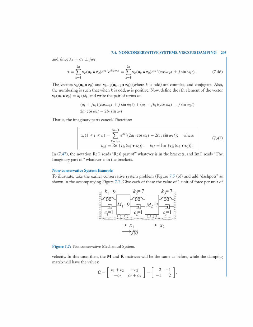
7.4. NONCONSERVATIVE SYSTEMS. VISCOUS DAMPING 205
and since λk = σk ± jωk
z =2n∑
k=1
vk(uk • z0)eσkt e±jωkt =
2n∑k=1
vk(uk • z0)eσkt (cos ωkt ± j sin ωkt) . (7.46)
The vectors vk(uk • z0) and vk+1(uk+1 • z0) (where k is odd) are complex, and conjugate. Also,the numbering is such that when k is odd, ω is positive. Now, define the ith element of the vectorvk(uk • z0) ≡ ai+jbi , and write the pair of terms as:
(ai + jbi)(cos ωkt + j sin ωkt) + (ai − jbi)(cos ωkt − j sin ωkt)
2ai cos ωit − 2bi sin ωit
That is, the imaginary parts cancel. Therefore:
xi(1 ≤ i ≤ n) =2n−1∑k=1,3
eσkt (2aki cos ωkt − 2bki sin ωkt); where
aki = Re {vki(uk • z0)} ; bki = Im {vki(uk • z0)} .
(7.47)
In (7.47), the notation Re{} reads “Real part of ” whatever is in the brackets, and Im{} reads “TheImaginary part of ” whatever is in the brackets.
Non-conservative System ExampleTo illustrate, take the earlier conservative system problem (Figure 7.5 (b)) and add “dashpots” asshown in the accompanying Figure 7.7. Give each of these the value of 1 unit of force per unit of
Figure 7.7: Nonconservative Mechanical System.
velocity. In this case, then, the M and K matrices will be the same as before, while the dampingmatrix will have the values:
C =[
c1 + c2 −c2
−c2 c2 + c3
]=[
2 −1−1 2
].
206 7. MATRIX ANALYSIS OF VIBRATING SYSTEMS
Following the methods previously discussed, the defining equation is Mx + Cx + Kx = 0, for theinitial value problem. The reduced (1st order) equation set is given by Equation (7.42) with the Amatrix:
A =[
0 IM−1K −M−1C
]=
⎡⎢⎢⎢⎣
0 0 1 00 0 0 1
− 169
79 − 2
919
1 −2 17 − 2
7
⎤⎥⎥⎥⎦ (7.48)
The analysis of A yields the eigenvalues and eigenvectors shown below.
Eigenvalues: λ1,2 = −0.06250 ± j0.99811; λ3,4 = −0.19147 ± j1.65552
Row Eigenvectors, U Column Eigenvectors, V
∥∥∥∥∥∥∥∥∥∥∥∥∥∥∥∥∥∥
−0.00587 −0.02761 −0.60194 −0.46775−0.60314 −0.46647 −0.02350 −0.00994
−0.00587 −0.02761 −0.60194 −0.467750.60314 0.46647 0.02350 0.00994
0.05629 −0.04696 0.53062 −0.531710.88447 −0.88621 0.02174 −0.03752
0.05629 −0.04696 0.53062 −0.53171−0.88447 0.88621 −0.02174 0.03752
∥∥∥∥∥∥∥∥∥∥∥∥∥∥∥∥∥∥
∥∥∥∥∥∥∥∥∥∥∥∥∥∥∥∥∥∥
0.01102 0.01102 −0.01837 −0.018370.46837 −0.46837 −0.24716 0.24716
0.01931 0.01931 0.01429 0.014290.46742 −0.46742 0.31952 −0.31952
−0.46817 −0.46817 0.41270 0.41270−0.01828 0.01828 0.01691 −0.01691
−0.46775 −0.46775 −0.53171 −0.53171−0.00994 0.00994 −0.03752 0.03752
∥∥∥∥∥∥∥∥∥∥∥∥∥∥∥∥∥∥
It appears that the damping is quite “light” inasmuch as the (negative) real parts of the eigenvaluesare small. The frequencies of the undamped case were 1.0 and 5/3. Note that damping lowers thesefrequencies (to 0.998 and 1.655, respectively). In the eigenvector display, the imaginary parts areshown below the reals. For example, u11 = −0.00587 − j0.60314.
As a point of interest, note that the bottom 2 elements of the columns, vi , are equal to λi
times the top. The row vectors are those which will be dotted into the initial value vector, z0. Theyare displayed, here, in rows. They are also in complex conjugate pairs, but unlike the columns, thelast 2 elements are not λ times the first two elements.
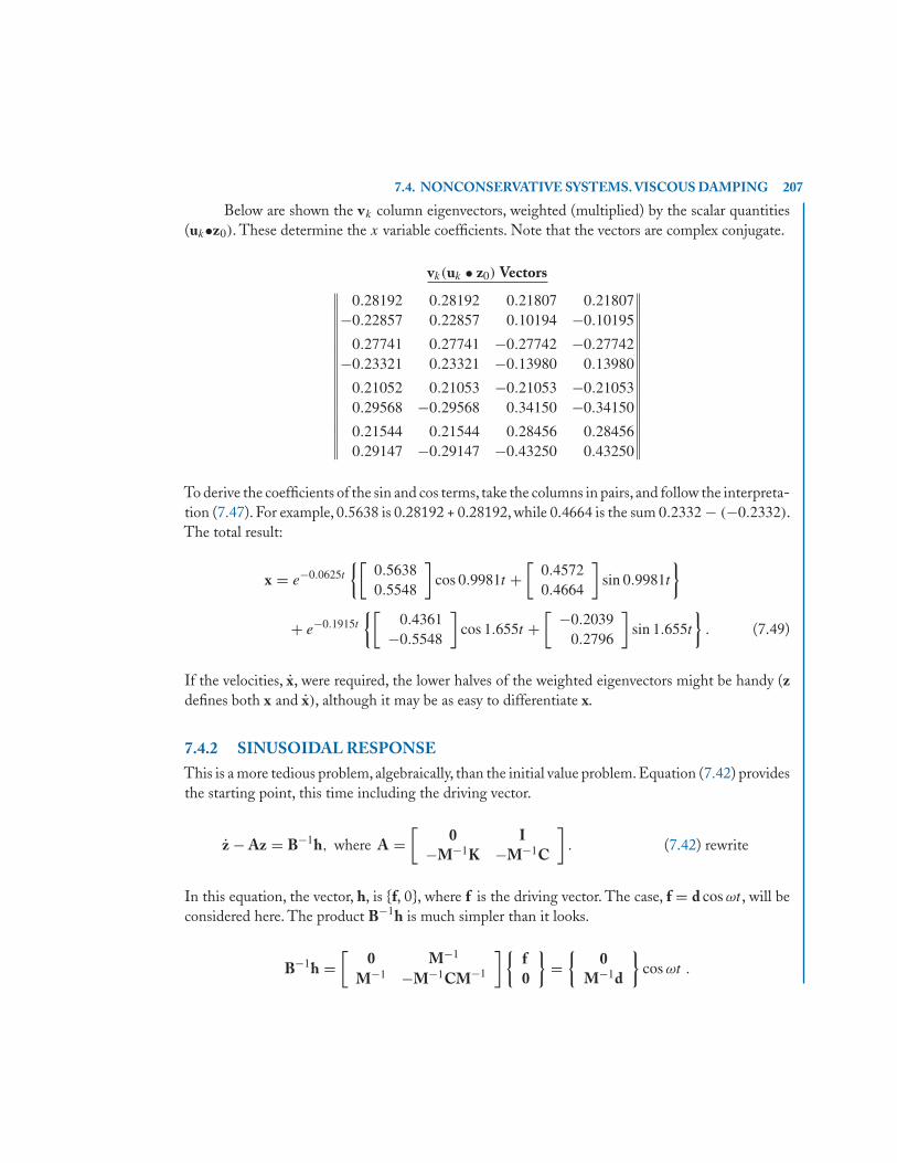
7.4. NONCONSERVATIVE SYSTEMS. VISCOUS DAMPING 207
Below are shown the vk column eigenvectors, weighted (multiplied) by the scalar quantities(uk•z0). These determine the x variable coefficients. Note that the vectors are complex conjugate.
vk(uk • z0) Vectors∥∥∥∥∥∥∥∥∥∥∥∥∥∥∥∥∥∥
0.28192 0.28192 0.21807 0.21807−0.22857 0.22857 0.10194 −0.10195
0.27741 0.27741 −0.27742 −0.27742−0.23321 0.23321 −0.13980 0.13980
0.21052 0.21053 −0.21053 −0.210530.29568 −0.29568 0.34150 −0.34150
0.21544 0.21544 0.28456 0.284560.29147 −0.29147 −0.43250 0.43250
∥∥∥∥∥∥∥∥∥∥∥∥∥∥∥∥∥∥To derive the coefficients of the sin and cos terms, take the columns in pairs, and follow the interpreta-tion (7.47). For example, 0.5638 is 0.28192 + 0.28192, while 0.4664 is the sum 0.2332 − (−0.2332).The total result:
x = e−0.0625t
{[0.56380.5548
]cos 0.9981t +
[0.45720.4664
]sin 0.9981t
}
+ e−0.1915t
{[0.4361
−0.5548
]cos 1.655t +
[ −0.20390.2796
]sin 1.655t
}. (7.49)
If the velocities, x, were required, the lower halves of the weighted eigenvectors might be handy (zdefines both x and x), although it may be as easy to differentiate x.
7.4.2 SINUSOIDAL RESPONSEThis is a more tedious problem, algebraically, than the initial value problem. Equation (7.42) providesthe starting point, this time including the driving vector.
z − Az = B−1h, where A =[
0 I−M−1K −M−1C
]. (7.42) rewrite
In this equation, the vector, h, is {f, 0}, where f is the driving vector. The case, f = d cos ωt , will beconsidered here. The product B−1h is much simpler than it looks.
B−1h =[
0 M−1
M−1 −M−1CM−1
]{f0
}={
0M−1d
}cos ωt .
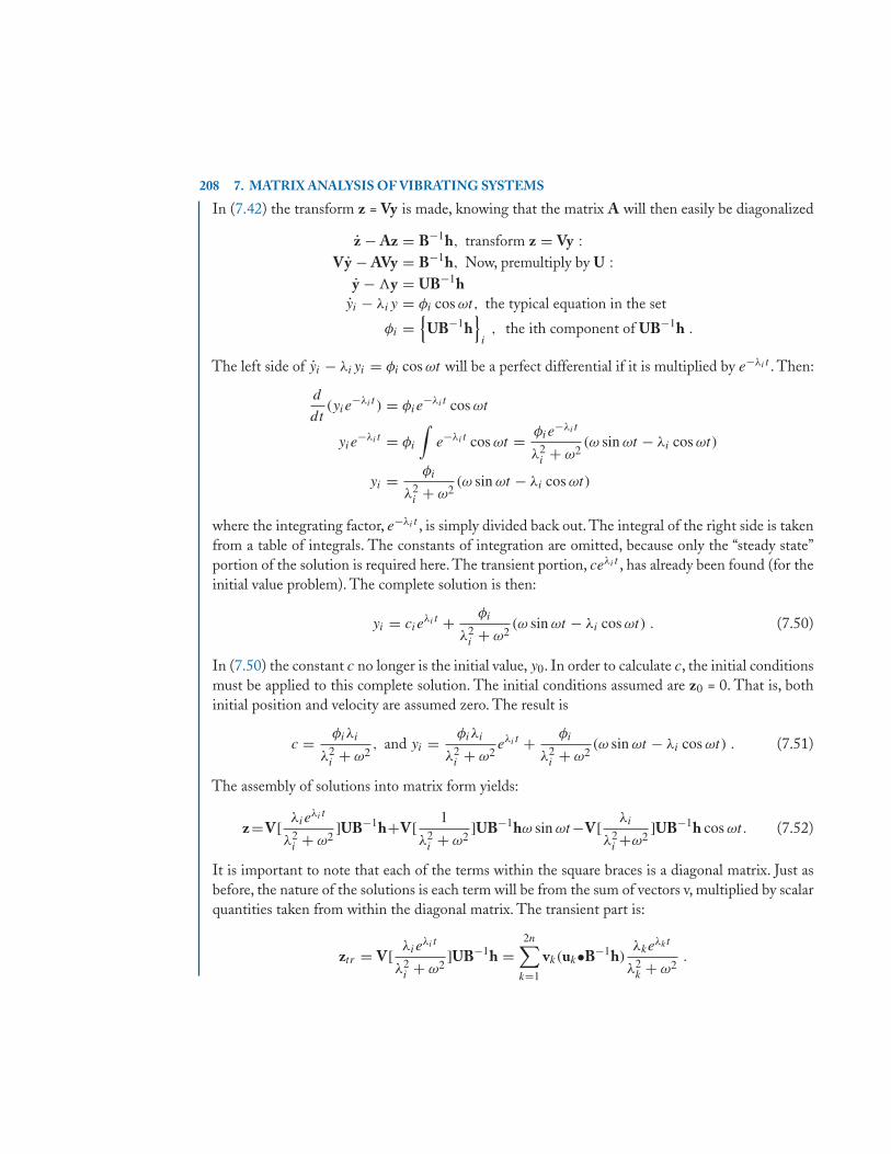
208 7. MATRIX ANALYSIS OF VIBRATING SYSTEMS
In (7.42) the transform z = Vy is made, knowing that the matrix A will then easily be diagonalized
z − Az = B−1h, transform z = Vy :Vy − AVy = B−1h, Now, premultiply by U :
y − �y = UB−1hyi − λiy = φi cos ωt, the typical equation in the set
φi ={
UB−1h}
i, the ith component of UB−1h .
The left side of yi − λiyi = φi cos ωt will be a perfect differential if it is multiplied by e−λi t . Then:
d
dt(yie
−λi t ) = φie−λi t cos ωt
yie−λi t = φi
∫e−λi t cos ωt = φie
−λi t
λ2i + ω2
(ω sin ωt − λi cos ωt)
yi = φi
λ2i + ω2
(ω sin ωt − λi cos ωt)
where the integrating factor, e−λi t , is simply divided back out. The integral of the right side is takenfrom a table of integrals. The constants of integration are omitted, because only the “steady state”portion of the solution is required here. The transient portion, ceλi t , has already been found (for theinitial value problem). The complete solution is then:
yi = cieλi t + φi
λ2i + ω2
(ω sin ωt − λi cos ωt) . (7.50)
In (7.50) the constant c no longer is the initial value, y0. In order to calculate c, the initial conditionsmust be applied to this complete solution. The initial conditions assumed are z0 = 0. That is, bothinitial position and velocity are assumed zero. The result is
c = φiλi
λ2i + ω2
, and yi = φiλi
λ2i + ω2
eλi t + φi
λ2i + ω2
(ω sin ωt − λi cos ωt) . (7.51)
The assembly of solutions into matrix form yields:
z =V[ λieλi t
λ2i + ω2
]UB−1h+V[ 1
λ2i + ω2
]UB−1hω sin ωt−V[ λi
λ2i +ω2
]UB−1h cos ωt. (7.52)
It is important to note that each of the terms within the square braces is a diagonal matrix. Just asbefore, the nature of the solutions is each term will be from the sum of vectors v, multiplied by scalarquantities taken from within the diagonal matrix. The transient part is:
ztr = V[ λieλi t
λ2i + ω2
]UB−1h =2n∑
k=1
vk(uk•B−1h)λke
λkt
λ2k + ω2
.
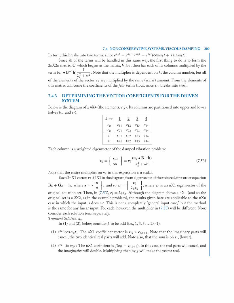
7.4. NONCONSERVATIVE SYSTEMS. VISCOUS DAMPING 209
In turn, this breaks into two terms, since eλkt = eσkt+jωkt = eσkt (cos ωkt + j sin ωkt).Since all of the terms will be handled in this same way, the first thing to do is to form the
2nX2n matrix, C, which begins as the matrix, V, but then has each of its columns multiplied by the
term (uk • B−1h)1
λ2k + ω2
. Note that the multiplier is dependent on k, the column number, but all
of the elements of the vector vk are multiplied by the same (scalar) amount. From the elements ofthis matrix will come the coefficients of the four terms (four, since ztr breaks into two).
7.4.3 DETERMINING THE VECTOR COEFFICIENTS FOR THE DRIVENSYSTEM
Below is the diagram of a 4X4 (the elements, cij ). Its columns are partitioned into upper and lowerhalves (cu and cl).
k �→ 1 2 3 4
cu c11 c12 c13 c14
cu c21 c22 c23 c24
cl c31 c32 c33 c34
cl c41 c42 c43 c44
Each column is a weighted eigenvector of the damped vibration problem:
ck ={
cuk
clk
}= vk
(uk • B−1h)
λ2k + ω2
. (7.53)
Note that the entire multiplier on vk in this expression is a scalar.Each 2nX1 vector,vk , (4X1 in the diagram) is an eigenvector of the reduced,first order equation
Bz + Gz = h, where z ={
xx
}, and so vk =
{ek
λkek
}, where ek is an nX1 eigenvector of the
original equation set. Then, in (7.53), cl = λkcu. Although the diagram shows a 4X4 (and so theoriginal set is a 2X2, as in the example problem), the results given here are applicable to the nXncase in which the input is dcos ωt . This is not a completely “general input case,” but the methodis the same for any linear input. For each, however, the multiplier in (7.53) will be different. Now,consider each solution term separately.Transient Solution, xtr
In (1) and (2), below, consider k to be odd (i.e., 1, 3, 5, …2n-1).
(1) eσkt cos ωkt : The nX1 coefficient vector is clk + cl,k+1. Note that the imaginary parts willcancel, the two identical real parts will add. Note also, that the sum is on cl , (lower).
(2) eσkt sin ωkt : The nX1 coefficient is j (clk − cl,k+1). In this case, the real parts will cancel, andthe imaginaries will double. Multiplying then by j will make the vector real.
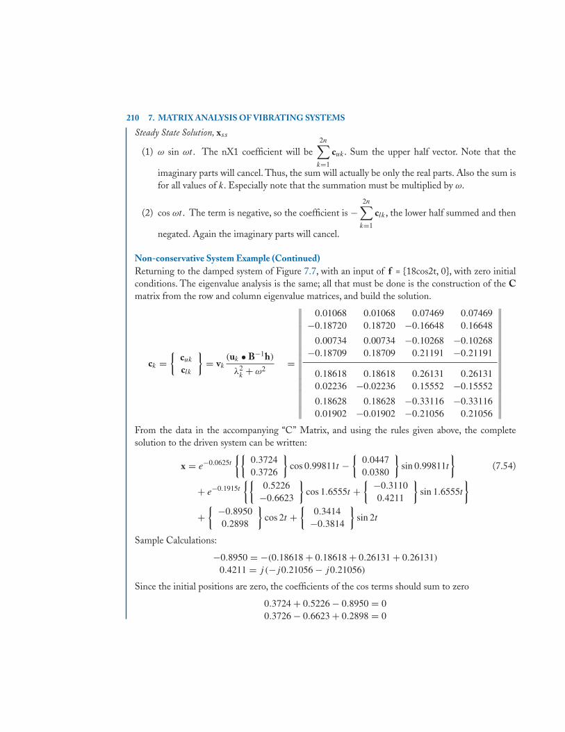
210 7. MATRIX ANALYSIS OF VIBRATING SYSTEMS
Steady State Solution, xss
(1) ω sin ωt . The nX1 coefficient will be2n∑
k=1
cuk . Sum the upper half vector. Note that the
imaginary parts will cancel. Thus, the sum will actually be only the real parts. Also the sum isfor all values of k. Especially note that the summation must be multiplied by ω.
(2) cos ωt . The term is negative, so the coefficient is −2n∑
k=1
clk , the lower half summed and then
negated. Again the imaginary parts will cancel.
Non-conservative System Example (Continued)Returning to the damped system of Figure 7.7, with an input of f = {18cos2t, 0}, with zero initialconditions. The eigenvalue analysis is the same; all that must be done is the construction of the Cmatrix from the row and column eigenvalue matrices, and build the solution.
ck ={
cuk
clk
}= vk
(uk • B−1h)
λ2k + ω2
=
∥∥∥∥∥∥∥∥∥∥∥∥∥∥∥∥∥∥∥
0.01068 0.01068 0.07469 0.07469−0.18720 0.18720 −0.16648 0.16648
0.00734 0.00734 −0.10268 −0.10268−0.18709 0.18709 0.21191 −0.21191
0.18618 0.18618 0.26131 0.261310.02236 −0.02236 0.15552 −0.15552
0.18628 0.18628 −0.33116 −0.331160.01902 −0.01902 −0.21056 0.21056
∥∥∥∥∥∥∥∥∥∥∥∥∥∥∥∥∥∥∥From the data in the accompanying “C” Matrix, and using the rules given above, the completesolution to the driven system can be written:
x = e−0.0625t
{{0.37240.3726
}cos 0.99811t −
{0.04470.0380
}sin 0.99811t
}(7.54)
+ e−0.1915t
{{0.5226
−0.6623
}cos 1.6555t +
{ −0.31100.4211
}sin 1.6555t
}
+{ −0.8950
0.2898
}cos 2t +
{0.3414
−0.3814
}sin 2t
Sample Calculations:
−0.8950 = −(0.18618 + 0.18618 + 0.26131 + 0.26131)
0.4211 = j (−j0.21056 − j0.21056)
Since the initial positions are zero, the coefficients of the cos terms should sum to zero
0.3724 + 0.5226 − 0.8950 = 00.3726 − 0.6623 + 0.2898 = 0
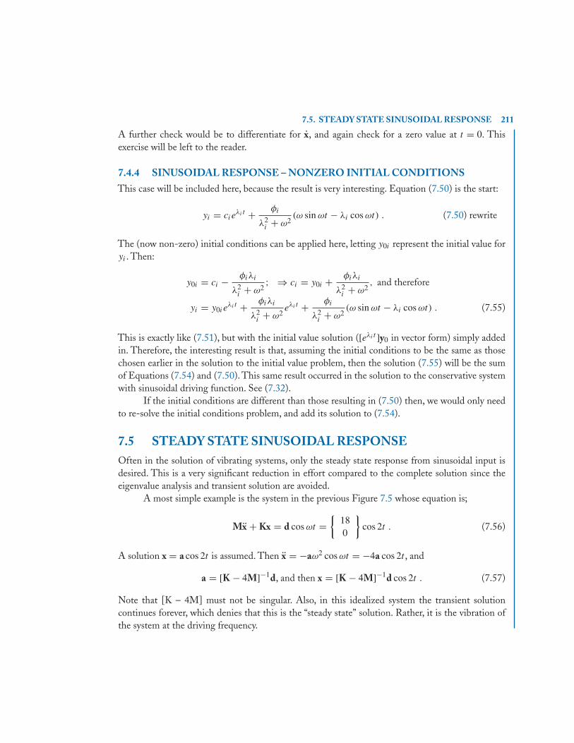
7.5. STEADY STATE SINUSOIDAL RESPONSE 211
A further check would be to differentiate for x, and again check for a zero value at t = 0. Thisexercise will be left to the reader.
7.4.4 SINUSOIDAL RESPONSE – NONZERO INITIAL CONDITIONSThis case will be included here, because the result is very interesting. Equation (7.50) is the start:
yi = cieλi t + φi
λ2i + ω2
(ω sin ωt − λi cos ωt) . (7.50) rewrite
The (now non-zero) initial conditions can be applied here, letting y0i represent the initial value foryi . Then:
y0i = ci − φiλi
λ2i + ω2
; ⇒ ci = y0i + φiλi
λ2i + ω2
, and therefore
yi = y0ieλi t + φiλi
λ2i + ω2
eλi t + φi
λ2i + ω2
(ω sin ωt − λi cos ωt) . (7.55)
This is exactly like (7.51), but with the initial value solution ([eλi t ]y0 in vector form) simply addedin. Therefore, the interesting result is that, assuming the initial conditions to be the same as thosechosen earlier in the solution to the initial value problem, then the solution (7.55) will be the sumof Equations (7.54) and (7.50). This same result occurred in the solution to the conservative systemwith sinusoidal driving function. See (7.32).
If the initial conditions are different than those resulting in (7.50) then, we would only needto re-solve the initial conditions problem, and add its solution to (7.54).
7.5 STEADY STATE SINUSOIDAL RESPONSEOften in the solution of vibrating systems, only the steady state response from sinusoidal input isdesired. This is a very significant reduction in effort compared to the complete solution since theeigenvalue analysis and transient solution are avoided.
A most simple example is the system in the previous Figure 7.5 whose equation is;
Mx + Kx = d cos ωt ={
180
}cos 2t . (7.56)
A solution x = a cos 2t is assumed. Then x = −aω2 cos ωt = −4a cos 2t , and
a = [K − 4M]−1d, and then x = [K − 4M]−1d cos 2t . (7.57)
Note that [K – 4M] must not be singular. Also, in this idealized system the transient solutioncontinues forever, which denies that this is the “steady state” solution. Rather, it is the vibration ofthe system at the driving frequency.
212 7. MATRIX ANALYSIS OF VIBRATING SYSTEMS
Using the parameter values from Figure 7.5, it will be found that (7.57) agrees with thesinusoidal response part of the complete solution found on page 187:
x = V[� − ω2I]−1UM−1d cos 2t . (7.58)
When the system includes dissipative elements, the situation is more complicated. For example,let it be required to find the steady state response of the mechanical system in Figure 7.7. the nonconservative system whose complete solution is the example used in the text.
Mx + Cx + Kx = d cos 2t . (7.59)
Now, an assumed solution of a cos 2t will not do, because of the Cx term. But, in this case, the drivercan be changed to dejωt = d(cos ωt + j sin ωt). This introduces the required imaginary part to thedriver. With an assumed solution of aejωt , real and imaginary parts satisfy the equations separately— so that the real part of the result comes from the cos input while the imaginary comes from thej sin input. When the actualinput is just cos ωt, the output is taken to be the real part of the resultof the analysis:
(−Mω2 + Cjω + K)aejωt = dejωt
a = [K − ω2M + jωC]−1d
x = Re{aejωt } .
(7.60)
Where Re{ } reads “Real part of{ }.” Equations (7.59) and (7.60) are general: the matrices are nXn,defined in the same way as previously discussed, although the specific example is a 2X2 system. Theone complication is that the square nXn matrix to be inverted is now complex — and note that thevector, a(nX1), will then, be complex. In this example, using the parameters of Figure 7.7:
a ={ −0.8950 − j0.34145
0.28972 + j0.38137
}. (7.61)
When this column for a is plugged back into x = Re{aejωt } the result checks with the values given inthe steady state portion of the complete solution to the nonconservative system.(see Equation (7.55)).
Steady state response is often the requirement in electrical networks. For illustration, considerthe electrical network shown here, which is the analog of the nonconservative mechanical systemdiscussed above. The electrical network with these parameters is not very realistic with R in ohms,L in henries, and C in farads, but it will serve to illustrate the method. Then:
(Lp2 + Rp + S)q ={
180
}cos ωt; S = 1
C, and p ≡ d
dt. (7.62)
L1 = 9, L2 = 7, S1 = 9, S2 = 7, S3 = 7, and R1 = R2 = R3 = 1, and with e(t) = 18 cos ωt .
Let it be required to find the steady state output voltage, e2, over a range of frequencies of the input.From the analysis of the mechanical system, the two resonant frequencies are 1 rps and 1.667 rps for

7.5. STEADY STATE SINUSOIDAL RESPONSE 213
the conservative system and slightly less for the system with damping.A reasonable range, then wouldbe from about 1/2 rps to 2 rps. The example uses the same parameters as those in the mass-springsystem.
For ω = 2, the steady state solution to the set is identical to that given for the nonconservativemechanical system except it results in the charges q1 and q2,, which will have to be differentiated(multiplied by jω) to obtain the current values, i. In this example, only i2 is of concern since i2R3 isequal to the voltage output desired. Using numbers from (7.61), above:
i = Re{jωaejωt }a = [S − ω2L + jωR]−1d
(7.63)
e2 = i2R3 = (0.28975 + j0.38137)jωejωt = (−0.76274 + j0.5795)ej2t .
It is common to write this result as an amplitude and phase angle. The amplitude is the sum of thesquares of these numbers (0.91759), then
e2 = 0.91759(−0.76274
0.91759+ j
0.5795
0.91759)ejωt = 0.91759ejϕejωt
e2 = 0.91759ej (ωt+ϕ); ϕ = tan−1 0.5795
−0.76274= 2.49rad = 142.7◦ . (7.64)
The objective, now, is to repeat this same solution, but using ω over the range 1/2 rps to 2 rps.The results are shown below.The greatest amplitude comes near the lower resonant frequency,
and there is hardly any increase in magnitude at the upper resonant frequency.The chart was created by stepping the driving frequency from 0.5 rps to 2.5 rps in 0.05
increments (fewer increments could have been used). At each frequency, the 2X2 complex matrix isinverted and premultiplied into the d vector, {18, 0}; in total there were a large number of operations— done by PC computer (in milliseconds).
In the following paragraphs, this same problem (i.e.,finding amplitude and phase of the outputover the same range of frequencies) will be accomplished a different way, and using a “special” typeof determinant.
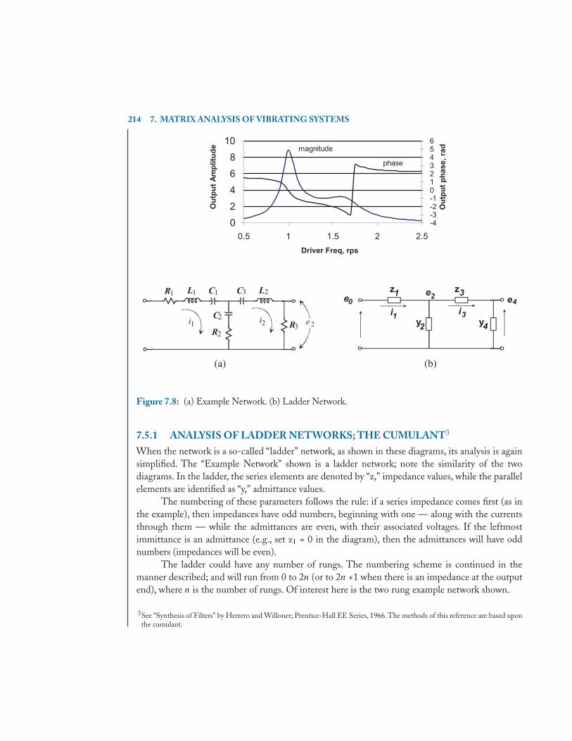
214 7. MATRIX ANALYSIS OF VIBRATING SYSTEMS
Figure 7.8: (a) Example Network. (b) Ladder Network.
7.5.1 ANALYSIS OF LADDER NETWORKS; THE CUMULANT3
When the network is a so-called “ladder” network, as shown in these diagrams, its analysis is againsimplified. The “Example Network” shown is a ladder network; note the similarity of the twodiagrams. In the ladder, the series elements are denoted by “z,” impedance values, while the parallelelements are identified as “y,” admittance values.
The numbering of these parameters follows the rule: if a series impedance comes first (as inthe example), then impedances have odd numbers, beginning with one — along with the currentsthrough them — while the admittances are even, with their associated voltages. If the leftmostimmittance is an admittance (e.g., set z1 = 0 in the diagram), then the admittances will have oddnumbers (impedances will be even).
The ladder could have any number of rungs. The numbering scheme is continued in themanner described; and will run from 0 to 2n (or to 2n +1 when there is an impedance at the outputend), where n is the number of rungs. Of interest here is the two rung example network shown.
3See “Synthesis of Filters” by Herrero and Willoner; Prentice-Hall EE Series, 1966. The methods of this reference are based uponthe cumulant.
7.5. STEADY STATE SINUSOIDAL RESPONSE 215
Comparing the two diagrams, z1 will be equal to. R1 + L1jω + S
jωfor steady state analysis.
The other immittances are calculated in the same manner. The voltages across the top of the ladderare related, and the currents summed in the ladder rungs, by Kirchhoff ’s laws. This results in thefollowing equation set:
e0 = i1z1 + e2
i1 − i3 = e2y2
e2 = i3z3 + e4
i3 = e4y4 .
in matrix format:
⎡⎢⎢⎣
z1 1 0 0−1 y2 1 0
0 −1 z3 10 0 −1 y4
⎤⎥⎥⎦⎧⎪⎪⎨⎪⎪⎩
i1
e2
i3
e4
⎫⎪⎪⎬⎪⎪⎭ =
⎧⎪⎪⎨⎪⎪⎩
e0
000
⎫⎪⎪⎬⎪⎪⎭ . (7.65)
These equations are written for the example problem, but the point is the form of the matrix in (7.65).It has the immittance values on the main diagonal (from 1 to 2n), with “1’s” in the upper codiagonal,and “-1’s” in the lower. The determinant, D, of this matrix is called a “cumulant.” With such astructured form, and so many zeros, it is not surprising that the cumulant is “special.” For example,its numeric value, given the values of the diagonal elements, is easily calculated by the followingalgorithm:
Let the main diagonal elements be designated a1, a2, · · · a2n. Then, the determinant valueis found by:
a [0] := 1 + j0;for k := 1 to 2*n dobegina[k] := {calculate the immittance value here}if k > 1 then a[k] := a[k]*a[k-1] + a[k-2];
end;D := a[k] {Note: D is the determinant value}
This algorithm assumes that a separate function (unique for every ladder network) is coded tocalculate the a[k] values — i.e., the (complex) immittances that lie along the main diagonal of thematrix in (7.65). This code is executed for each frequency value. The separate function calculates animpedance value for k-odd, or an admittance value for k-even. For the example network, when k =
1, the function would return the complex number: R1 + j (L1ω − S1
ω).
Following Cramer’s Rule, the output voltage is found by replacing the 4th column in D withthe column on the right side of the Equation (7.65). This determinant, call it D4, expanded by the4th column elements, has the simple value, e0. Then:
e4 = D4
D= e0
D. (7.66)
In the example problem, e0 = 18. It will be found that this method produces the same results thatwere obtained, above.
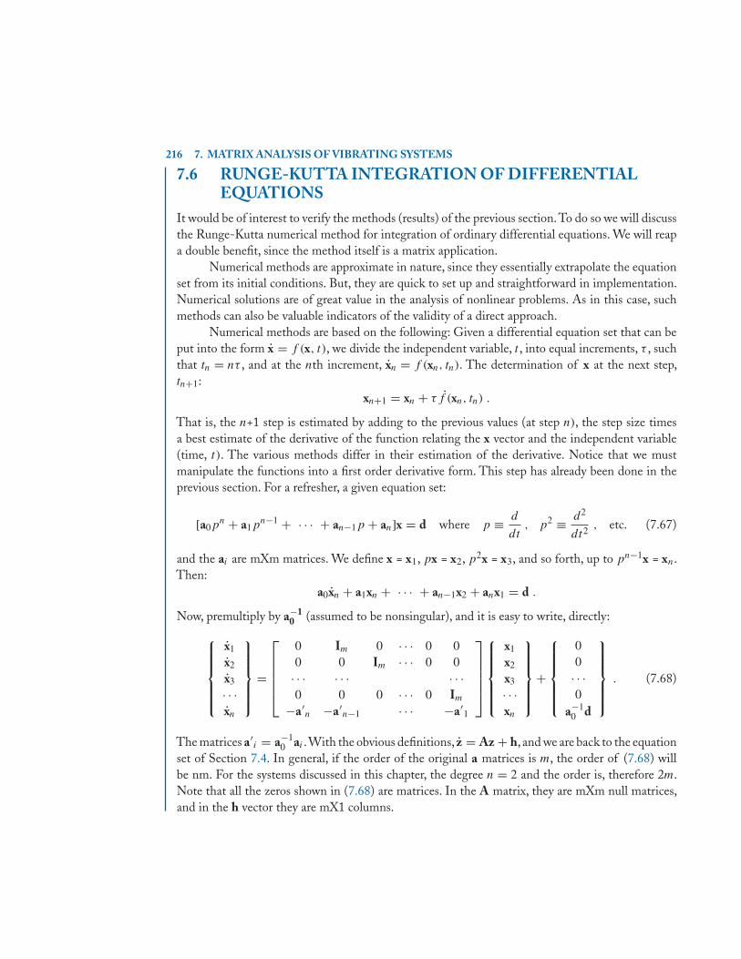
216 7. MATRIX ANALYSIS OF VIBRATING SYSTEMS
7.6 RUNGE-KUTTA INTEGRATION OF DIFFERENTIALEQUATIONS
It would be of interest to verify the methods (results) of the previous section.To do so we will discussthe Runge-Kutta numerical method for integration of ordinary differential equations. We will reapa double benefit, since the method itself is a matrix application.
Numerical methods are approximate in nature, since they essentially extrapolate the equationset from its initial conditions. But, they are quick to set up and straightforward in implementation.Numerical solutions are of great value in the analysis of nonlinear problems. As in this case, suchmethods can also be valuable indicators of the validity of a direct approach.
Numerical methods are based on the following: Given a differential equation set that can beput into the form x = f (x, t), we divide the independent variable, t , into equal increments, τ , suchthat tn = nτ , and at the nth increment, xn = f (xn, tn). The determination of x at the next step,tn+1:
xn+1 = xn + τ f (xn, tn) .
That is, the n+1 step is estimated by adding to the previous values (at step n), the step size timesa best estimate of the derivative of the function relating the x vector and the independent variable(time, t). The various methods differ in their estimation of the derivative. Notice that we mustmanipulate the functions into a first order derivative form. This step has already been done in theprevious section. For a refresher, a given equation set:
[a0pn + a1p
n−1 + · · · + an−1p + an]x = d where p ≡ d
dt, p2 ≡ d2
dt2, etc. (7.67)
and the ai are mXm matrices. We define x = x1, px = x2, p2x = x3, and so forth, up to pn−1x = xn.Then:
a0xn + a1xn + · · · + an−1x2 + anx1 = d .
Now, premultiply by a−10 (assumed to be nonsingular), and it is easy to write, directly:
⎧⎪⎪⎪⎪⎨⎪⎪⎪⎪⎩
x1
x2
x3
· · ·xn
⎫⎪⎪⎪⎪⎬⎪⎪⎪⎪⎭
=
⎡⎢⎢⎢⎢⎣
0 Im 0 · · · 0 00 0 Im · · · 0 0· · · · · · · · ·0 0 0 · · · 0 Im
−a′n −a′
n−1 · · · −a′1
⎤⎥⎥⎥⎥⎦
⎧⎪⎪⎪⎪⎨⎪⎪⎪⎪⎩
x1
x2
x3
· · ·xn
⎫⎪⎪⎪⎪⎬⎪⎪⎪⎪⎭
+
⎧⎪⎪⎪⎪⎨⎪⎪⎪⎪⎩
00· · ·0
a−10 d
⎫⎪⎪⎪⎪⎬⎪⎪⎪⎪⎭
. (7.68)
The matrices a′i = a−1
0 ai .With the obvious definitions, z = Az + h, and we are back to the equationset of Section 7.4. In general, if the order of the original a matrices is m, the order of (7.68) willbe nm. For the systems discussed in this chapter, the degree n = 2 and the order is, therefore 2m.Note that all the zeros shown in (7.68) are matrices. In the A matrix, they are mXm null matrices,and in the h vector they are mX1 columns.
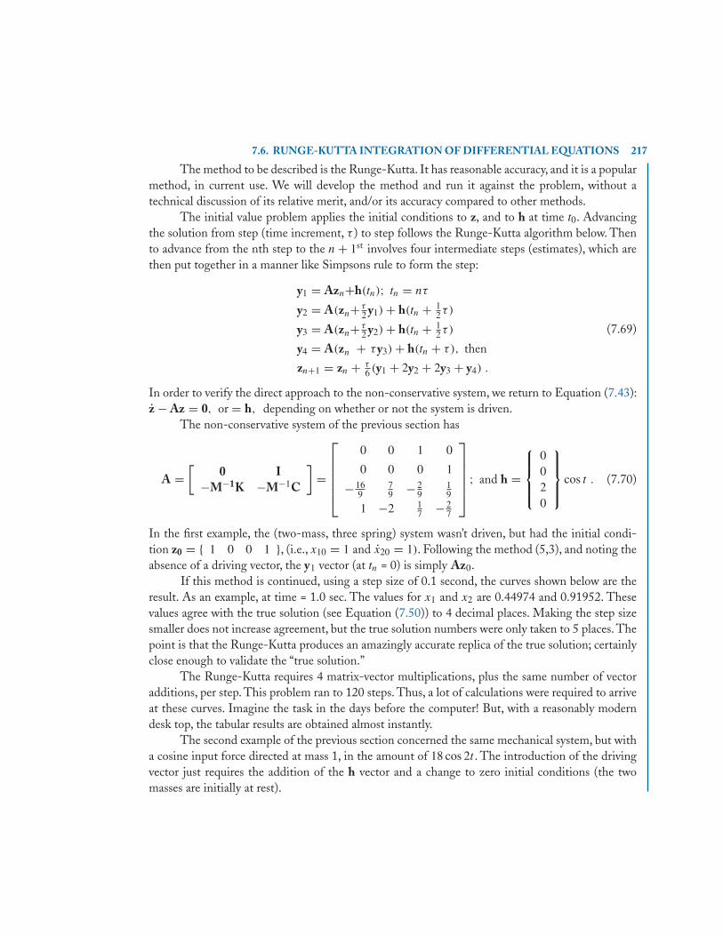
7.6. RUNGE-KUTTA INTEGRATION OF DIFFERENTIAL EQUATIONS 217
The method to be described is the Runge-Kutta. It has reasonable accuracy, and it is a popularmethod, in current use. We will develop the method and run it against the problem, without atechnical discussion of its relative merit, and/or its accuracy compared to other methods.
The initial value problem applies the initial conditions to z, and to h at time t0. Advancingthe solution from step (time increment, τ ) to step follows the Runge-Kutta algorithm below. Thento advance from the nth step to the n + 1st involves four intermediate steps (estimates), which arethen put together in a manner like Simpsons rule to form the step:
y1 = Azn+h(tn); tn = nτ
y2 = A(zn+ τ2 y1) + h(tn + 1
2τ)
y3 = A(zn+ τ2 y2) + h(tn + 1
2τ)
y4 = A(zn + τy3) + h(tn + τ), then
zn+1 = zn + τ6 (y1 + 2y2 + 2y3 + y4) .
(7.69)
In order to verify the direct approach to the non-conservative system, we return to Equation (7.43):z − Az = 0, or = h, depending on whether or not the system is driven.
The non-conservative system of the previous section has
A =[
0 I−M−1K −M−1C
]=
⎡⎢⎢⎢⎢⎣
0 0 1 0
0 0 0 1
− 169
79 − 2
919
1 −2 17 − 2
7
⎤⎥⎥⎥⎥⎦ ; and h =
⎧⎪⎪⎨⎪⎪⎩
0020
⎫⎪⎪⎬⎪⎪⎭ cos t . (7.70)
In the first example, the (two-mass, three spring) system wasn’t driven, but had the initial condi-tion z0 = { 1 0 0 1 }, (i.e., x10 = 1 and x20 = 1). Following the method (5,3), and noting theabsence of a driving vector, the y1 vector (at tn = 0) is simply Az0.
If this method is continued, using a step size of 0.1 second, the curves shown below are theresult. As an example, at time = 1.0 sec. The values for x1 and x2 are 0.44974 and 0.91952. Thesevalues agree with the true solution (see Equation (7.50)) to 4 decimal places. Making the step sizesmaller does not increase agreement, but the true solution numbers were only taken to 5 places. Thepoint is that the Runge-Kutta produces an amazingly accurate replica of the true solution; certainlyclose enough to validate the “true solution.”
The Runge-Kutta requires 4 matrix-vector multiplications, plus the same number of vectoradditions, per step. This problem ran to 120 steps. Thus, a lot of calculations were required to arriveat these curves. Imagine the task in the days before the computer! But, with a reasonably moderndesk top, the tabular results are obtained almost instantly.
The second example of the previous section concerned the same mechanical system, but witha cosine input force directed at mass 1, in the amount of 18 cos 2t . The introduction of the drivingvector just requires the addition of the h vector and a change to zero initial conditions (the twomasses are initially at rest).
218 7. MATRIX ANALYSIS OF VIBRATING SYSTEMS
Over a 12 second time period, with a step size of 0.1 sec, the results again agree with the truesolution in the first 4 decimals.
The graph below plots the motion of the two masses.
7.7 EXERCISES
7.1. Reduce the equation, ax + bx + cx + dx = f (t) to a set of 1st order equations.
7.2. The single spring-mass system (a) shown below, has the natural frequency
ω =√
km
(system restricted to vertical motion) .
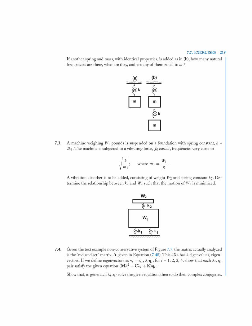
7.7. EXERCISES 219
If another spring and mass, with identical properties, is added as in (b), how many naturalfrequencies are there, what are they, and are any of them equal to ω ?
7.3. A machine weighing W1 pounds is suspended on a foundation with spring constant, k =2k1. The machine is subjected to a vibrating force, f0 cos ωt , frequencies very close to
√k
m1; where m1 = W1
g.
A vibration absorber is to be added, consisting of weight W2 and spring constant k2. De-termine the relationship between k2 and W2 such that the motion of W1 is minimized.
7.4. Given the text example non-conservative system of Figure 7.7, the matrix actually analyzedis the “reduced set” matrix, A, given in Equation (7.48). This 4X4 has 4 eigenvalues, eigen-vectors. If we define eigenvectors as vi = qi , λiqi , for i = 1, 2, 3, 4, show that each λi, qi
pair satisfy the given equation (Mλ2i + Cλi + K)qi .
Show that, in general, if λi , qi solve the given equation, then so do their complex conjugates.
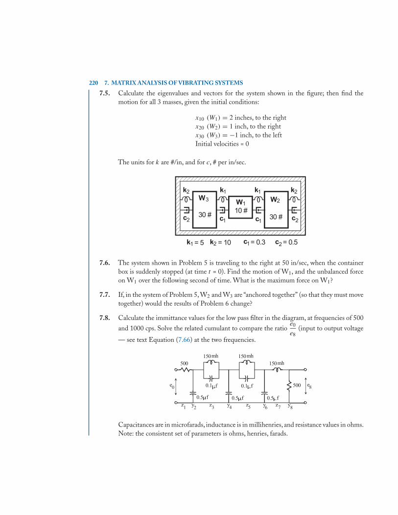
220 7. MATRIX ANALYSIS OF VIBRATING SYSTEMS
7.5. Calculate the eigenvalues and vectors for the system shown in the figure; then find themotion for all 3 masses, given the initial conditions:
x10 (W1) = 2 inches, to the rightx20 (W2) = 1 inch, to the rightx30 (W3) = −1 inch, to the leftInitial velocities = 0
The units for k are #/in, and for c, # per in/sec.
7.6. The system shown in Problem 5 is traveling to the right at 50 in/sec, when the containerbox is suddenly stopped (at time t = 0). Find the motion of W1, and the unbalanced forceon W1 over the following second of time. What is the maximum force on W1?
7.7. If, in the system of Problem 5, W2 and W3 are “anchored together” (so that they must movetogether) would the results of Problem 6 change?
7.8. Calculate the immittance values for the low pass filter in the diagram, at frequencies of 500
and 1000 cps. Solve the related cumulant to compare the ratioe0
e8(input to output voltage
— see text Equation (7.66) at the two frequencies.
Capacitances are in microfarads, inductance is in millihenries, and resistance values in ohms.Note: the consistent set of parameters is ohms, henries, farads.
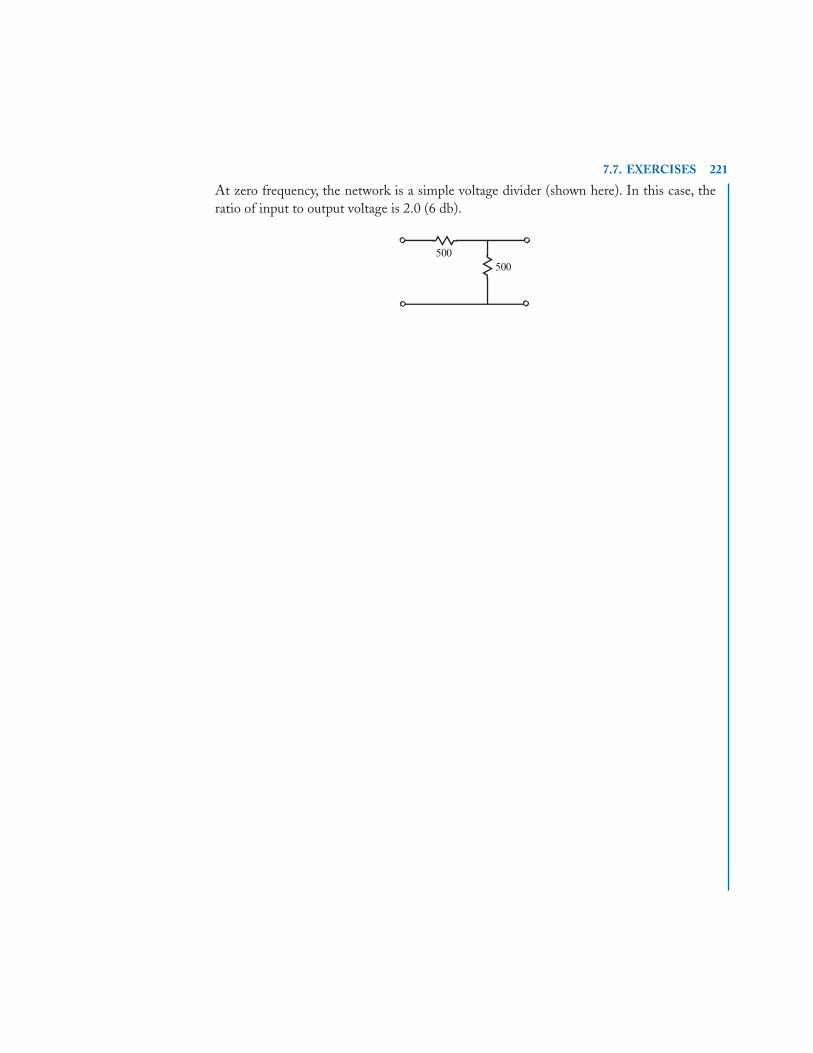
7.7. EXERCISES 221
At zero frequency, the network is a simple voltage divider (shown here). In this case, theratio of input to output voltage is 2.0 (6 db).

223
A P P E N D I X A
Partial Differentiation ofBilinear and Quadratic Forms
Begin with the definition of the partial differential operator, “del,” ∇. This operator is defined as acolumn vector, an (mX1) matrix:
∇ =
⎧⎪⎪⎪⎪⎪⎪⎪⎪⎪⎨⎪⎪⎪⎪⎪⎪⎪⎪⎪⎩
∂
∂ x1
∂
∂ x2...
∂
∂ xm
⎫⎪⎪⎪⎪⎪⎪⎪⎪⎪⎬⎪⎪⎪⎪⎪⎪⎪⎪⎪⎭
. (A.1)
The column length is determined by the number of independent variables, (x1, x2, · · · xm), there arem of these, and del should be written ∇x . indicating the independent variable. Herein, the subscriptwill be omitted unless there could be a confusion.
Note that ∇ is an operator; it is meaningless standing alone (A.1). But, given a functionq(x1, x2, . . . xm):
∇q = ∇q(x1, x2, · · · xm) =
⎧⎪⎪⎪⎪⎪⎪⎪⎪⎪⎨⎪⎪⎪⎪⎪⎪⎪⎪⎪⎩
∂ q
∂ x1
∂ q
∂ x2...
∂ q
∂ xm
⎫⎪⎪⎪⎪⎪⎪⎪⎪⎪⎬⎪⎪⎪⎪⎪⎪⎪⎪⎪⎭
(A.2)
certainly is meaningful, it being all the partials of q arranged into a column vector. As with alloperators, one must be careful with the order in which the symbols are written. q∇ is as meaninglessas ∇ itself.
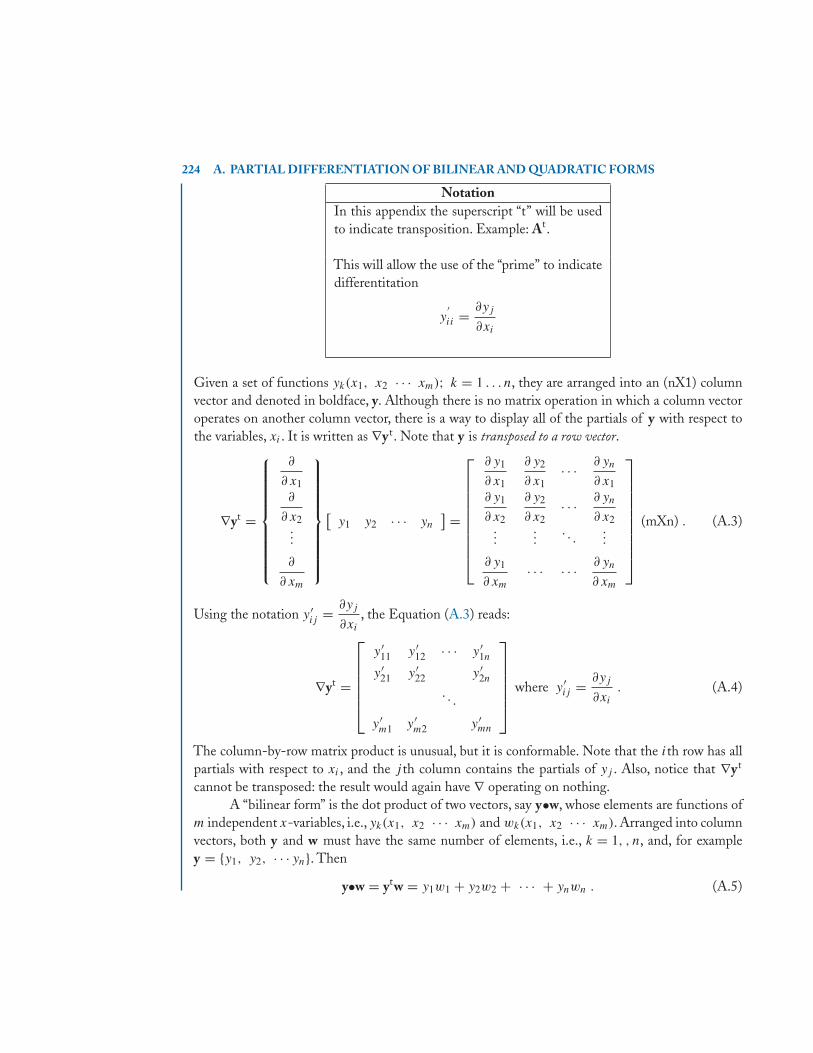
224 A. PARTIAL DIFFERENTIATION OF BILINEAR AND QUADRATIC FORMS
NotationIn this appendix the superscript “t” will be usedto indicate transposition. Example: At.
This will allow the use of the “prime” to indicatedifferentitation
y′ii = ∂yj
∂xi
Given a set of functions yk(x1, x2 · · · xm); k = 1 . . . n, they are arranged into an (nX1) columnvector and denoted in boldface, y. Although there is no matrix operation in which a column vectoroperates on another column vector, there is a way to display all of the partials of y with respect tothe variables, xi . It is written as ∇yt. Note that y is transposed to a row vector.
∇yt =
⎧⎪⎪⎪⎪⎪⎪⎪⎪⎪⎨⎪⎪⎪⎪⎪⎪⎪⎪⎪⎩
∂
∂ x1∂
∂ x2...
∂
∂ xm
⎫⎪⎪⎪⎪⎪⎪⎪⎪⎪⎬⎪⎪⎪⎪⎪⎪⎪⎪⎪⎭
[y1 y2 · · · yn
] =
⎡⎢⎢⎢⎢⎢⎢⎢⎢⎢⎣
∂ y1
∂ x1
∂ y2
∂ x1· · · ∂ yn
∂ x1∂ y1
∂ x2
∂ y2
∂ x2· · · ∂ yn
∂ x2...
.... . .
...
∂ y1
∂ xm
· · · · · · ∂ yn
∂ xm
⎤⎥⎥⎥⎥⎥⎥⎥⎥⎥⎦
(mXn) . (A.3)
Using the notation y′ij = ∂yj
∂xi
, the Equation (A.3) reads:
∇yt =
⎡⎢⎢⎢⎢⎢⎣
y′11 y′
12 · · · y′1n
y′21 y′
22 y′2n
. . .
y′m1 y′
m2 y′mn
⎤⎥⎥⎥⎥⎥⎦ where y′
ij = ∂yj
∂xi
. (A.4)
The column-by-row matrix product is unusual, but it is conformable. Note that the ith row has allpartials with respect to xi , and the j th column contains the partials of yj . Also, notice that ∇yt
cannot be transposed: the result would again have ∇ operating on nothing.A “bilinear form” is the dot product of two vectors, say y•w, whose elements are functions of
m independent x-variables, i.e., yk(x1, x2 · · · xm) and wk(x1, x2 · · · xm). Arranged into columnvectors, both y and w must have the same number of elements, i.e., k = 1, , n, and, for exampley = {y1, y2, · · · yn}. Then
y•w = ytw = y1w1 + y2w2 + · · · + ynwn . (A.5)
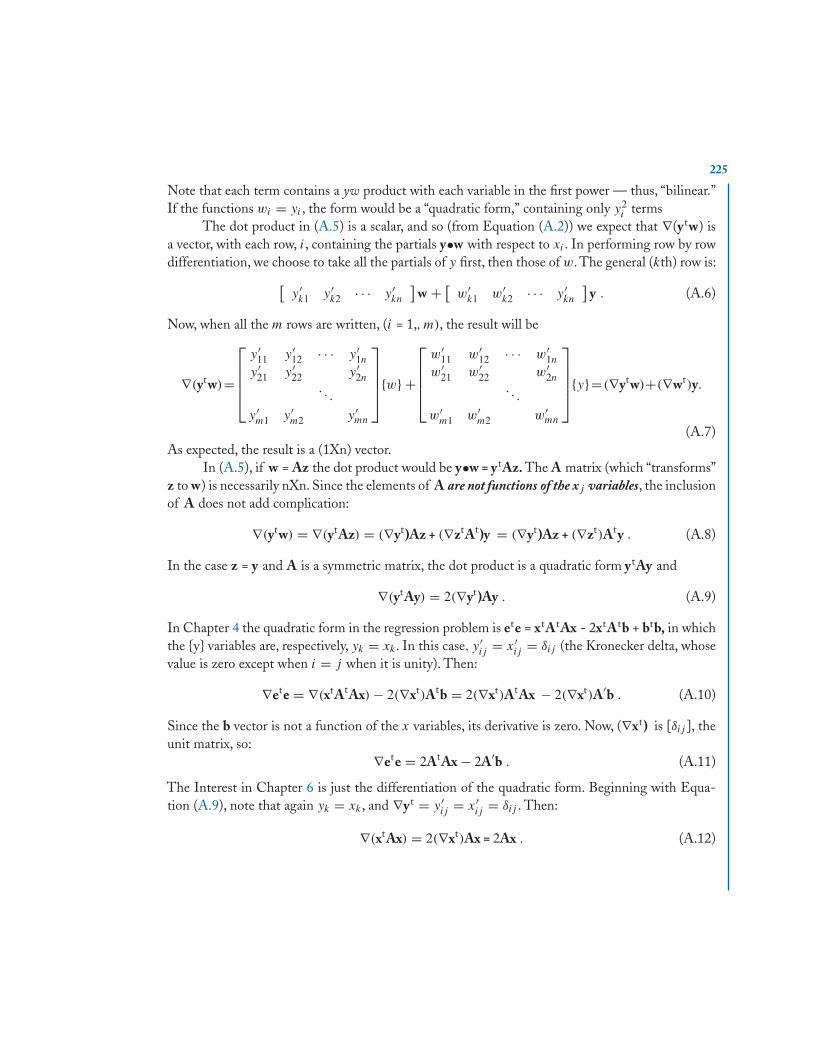
225
Note that each term contains a yw product with each variable in the first power — thus, “bilinear.”If the functions wi = yi , the form would be a “quadratic form,” containing only y2
i termsThe dot product in (A.5) is a scalar, and so (from Equation (A.2)) we expect that ∇(ytw) is
a vector, with each row, i, containing the partials y•w with respect to xi . In performing row by rowdifferentiation, we choose to take all the partials of y first, then those of w. The general (kth) row is:[
y′k1 y′
k2 · · · y′kn
]w + [
w′k1 w′
k2 · · · y′kn
]y . (A.6)
Now, when all the m rows are written, (i = 1,, m), the result will be
∇(ytw)=
⎡⎢⎢⎢⎣
y′11 y′
12 · · · y′1n
y′21 y′
22 y′2n
. . .
y′m1 y′
m2 y′mn
⎤⎥⎥⎥⎦{w} +
⎡⎢⎢⎢⎣
w′11 w′
12 · · · w′1n
w′21 w′
22 w′2n
. . .
w′m1 w′
m2 w′mn
⎤⎥⎥⎥⎦{y}=(∇ytw)+(∇wt)y.
(A.7)As expected, the result is a (1Xn) vector.
In (A.5), if w = Az the dot product would be y•w = ytAz. The A matrix (which “transforms”z to w) is necessarily nXn. Since the elements of A are not functions of the xj variables, the inclusionof A does not add complication:
∇(ytw) = ∇(ytAz) = (∇yt)Az + (∇ztAt)y = (∇yt)Az + (∇zt)Aty . (A.8)
In the case z = y and A is a symmetric matrix, the dot product is a quadratic form ytAy and
∇(ytAy) = 2(∇yt)Ay . (A.9)
In Chapter 4 the quadratic form in the regression problem is ete = xtAtAx - 2xtAtb + btb, in whichthe {y} variables are, respectively, yk = xk . In this case, y′
ij = x′ij = δij (the Kronecker delta, whose
value is zero except when i = j when it is unity). Then:
∇ete = ∇(xtAtAx) − 2(∇xt)Atb = 2(∇xt)AtAx − 2(∇xt)A′b . (A.10)
Since the b vector is not a function of the x variables, its derivative is zero. Now, (∇xt) is [δij ], theunit matrix, so:
∇ete = 2AtAx − 2A′b . (A.11)
The Interest in Chapter 6 is just the differentiation of the quadratic form. Beginning with Equa-tion (A.9), note that again yk = xk , and ∇yt = y′
ij = x′ij = δij . Then:
∇(xtAx) = 2(∇xt)Ax = 2Ax . (A.12)

227
A P P E N D I X B
PolynomialsAssociated with every square (nXn) matrix is a characteristic polynomial equation:
f (λ) = c0λn + c1λ
n−1 + · · · cn−1λ + cn = 0
whose degree is n. The roots of this polynomial are the eigenvalues of the matrix. Our interest inpolynomials is fueled by the requirement to find these eigenvalues. Toward that end, some of thebasic arithmetic algorithms are discussed here, with a display of “Pascal-like” code. Then, an outlineof a recommended method for determining polynomial roots is given.
B.1 POLYNOMIAL BASICSIn this appendix the polynomial will be written as:
p(x) = c0xn + c1x
n−1 + · · · + cn−1x + cn = 0 . (B.1)
The coefficient, c0, the coefficient of the highest power term, can always be made to equal unity. Onlyc0 and cn are required to be non-zero and both c0 and cn can be made unity by the transformation
x = kz with k = n
√cn
c0. Note that in the representation, (B.1), the sum of the subscript on each term
with its corresponding power always equals n.The Equation (B.1) is not an identity; there are exactly n (generally complex) “roots,” xj ,
that cause p(x) to vanish. In this discussion, we consider only polynomials with real coefficients. Asa consequence, if a root is complex, its complex conjugate must also be a root. If the degree, n, is odd,there must be at least one real root.
It is sometimes desirable to define a related polynomial, defined by the transform x = 1/z:
p(z) = cnzn + cn−1z
n−1 + · · · + c1z + c0 = 0 (B.2)
which is the same as (B.1), but with the coefficients taken in reverse order, and possessing theinverses of the roots of (B.1). A root x > 1 is transformed to a root z < 1. As an example, if the rootextraction method converges to the smallest (absolute value) root first, then (B.2) might be used toobtain roots in the reverse order.
Denoting the roots of (B.1) as xj , j = 1..n, the polynomial can be written as in (B.3):
p(x) =n∏
j=1
(x − xj ) = (x − x1)(x − x2) · · · (x − xn) . (B.3)
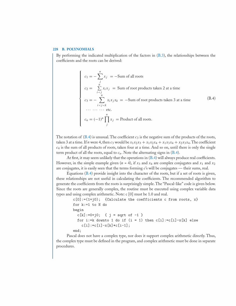
228 B. POLYNOMIALS
By performing the indicated multiplication of the factors in (B.3), the relationships between thecoefficients and the roots can be derived:
⎧⎪⎪⎪⎪⎪⎪⎪⎪⎪⎪⎪⎪⎪⎪⎪⎪⎪⎨⎪⎪⎪⎪⎪⎪⎪⎪⎪⎪⎪⎪⎪⎪⎪⎪⎪⎩
c1 = −n∑j
xj = −Sum of all roots
c2 =n∑
i<j
xixj = Sum of root products taken 2 at a time
c3 = −n∑
i<j<k
xixjxk = −Sum of root products taken 3 at a time
· · · · · · · · · etc.
cn = (−1)nn∏j
xj = Product of all roots.
(B.4)
The notation of (B.4) is unusual. The coefficient c3 is the negative sum of the products of the roots,taken 3 at a time. If n were 4, then c3 would be x1x2x3 + x1x2x4 + x1x3x4 + x2x3x4.The coefficientc4 is the sum of all products of roots, taken four at a time. And so on, until there is only the singleterm product of all the roots, equal to cn. Note the alternating signs in (B.4).
At first, it may seem unlikely that the operations in (B.4) will always produce real coefficients.However, in the simple example given (n = 4), if x3 and x4 are complex conjugates and x1 and x2
are conjugates, it is easily seen that the terms forming c’s will be conjugates — their sums, real.Equations (B.4) provide insight into the character of the roots, but if a set of roots is given,
these relationships are not useful in calculating the coefficients. The recommended algorithm togenerate the coefficients from the roots is surprisingly simple. The “Pascal-like” code is given below.Since the roots are generally complex, the routine must be executed using complex variable datatypes and using complex arithmetic. Note: c [0] must be 1.0 and real.
c[0]:=(1+j0); {Calculate the coefficients c from roots, x}for k:=1 to N dobeginc[k]:=0+j0; { j = sqrt of -1 }for i:=k downto 1 do if (i = 1) then c[i]:=c[i]-x[k] elsec[i]:=c[i]-x[k]*c[i-1];
end;Pascal does not have a complex type, nor does it support complex arithmetic directly. Thus,
the complex type must be defined in the program, and complex arithmetic must be done in separateprocedures.
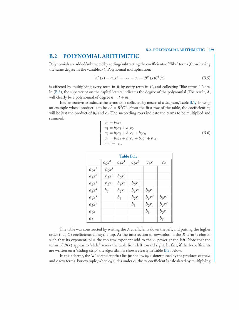
B.2. POLYNOMIAL ARITHMETIC 229
B.2 POLYNOMIAL ARITHMETICPolynomials are added/subtracted by adding/subtracting the coefficients of “like” terms (those havingthe same degree in the variable, x). Polynomial multiplication:
An(x) = a0xn + · · · + an = Bm(x)Cl(x) (B.5)
is affected by multiplying every term in B by every term in C, and collecting “like terms.” Note,in (B.5), the superscript on the capital letters indicates the degree of the polynomial. The result, A,will clearly be a polynomial of degree n = l + m.
It is instructive to indicate the terms to be collected by means of a diagram,Table B.1, showingan example whose product is to be A7 = B3C4. From the first row of the table, the coefficient a0
will be just the product of b0 and c0. The succeeding rows indicate the terms to be multiplied andsummed: ⎧⎪⎪⎪⎪⎨
⎪⎪⎪⎪⎩
a0 = b0c0
a1 = b0c1 + b1c0
a2 = b0c2 + b1c1 + b2c0
a3 = b0c3 + b1c2 + b2c1 + b3c0
· · · = etc
(B.6)
Table B.1:
The table was constructed by writing the A coefficients down the left, and putting the higherorder (i.e., C) coefficients along the top. At the intersection of row/column, the B term is chosensuch that its exponent, plus the top row exponent add to the A power at the left. Note that theterms of B(x) appear to “slide” across the table from left toward right. In fact, if the b coefficientsare written on a “sliding strip” the algorithm is shown clearly in Table B.2, below.
In this scheme, the “a” coefficient that lies just below b0 is determined by the products of the b
and c row terms. For example, when b0 slides under c3 the a3 coefficient is calculated by multiplying
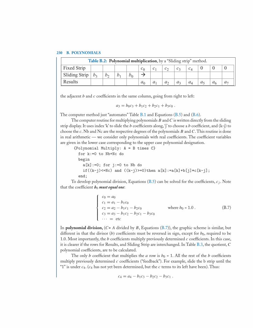
230 B. POLYNOMIALS
Table B.2: Polynomial multiplication, by a “Sliding strip” method.
the adjacent b and c coefficients in the same column, going from right to left:
a3 = b0c3 + b1c2 + b2c1 + b3c0 .
The computer method just “automates” Table B.1 and Equations (B.5) and (B.6).The computer routine for multiplying polynomials B and C is written directly from the sliding
strip display. It uses index ‘k’ to slide the b coefficients along, ‘j’ to choose a b coefficient, and (k-j) tochoose the c. Nb and Nc are the respective degrees of the polynomials B and C.This routine is donein real arithmetic — we consider only polynomials with real coefficients. The coefficient variablesare given in the lower case corresponding to the upper case polynomial designation.
{Polynomial Multiply: A = B times C}for k:=0 to Nb+Nc dobegina[k]:=0; for j:=0 to Nb doif((k-j)<=Nc) and ((k-j)>=0)then a[k]:=a[k]+b[j]*c[k-j];
end;To develop polynomial division, Equations (B.5) can be solved for the coefficients, cj . Note
that the coefficient b0 must equal one:⎧⎪⎪⎪⎪⎨⎪⎪⎪⎪⎩
c0 = a0
c1 = a1 − b1c0
c2 = a2 − b1c1 − b2c0
c3 = a3 − b1c2 − b2c1 − b3c0
· · · = etc
where b0 = 1.0 . (B.7)
In polynomial division, (C= A divided by B, Equations (B.7)), the graphic scheme is similar, butdifferent in that the divisor (b) coefficients must be reversed in sign, except for b0, required to be1.0. Most importantly, the b coefficients multiply previously determined c coefficients. In this case,it is clearer if the rows for Results, and Sliding Strip are interchanged. In Table B.3, the quotient, Cpolynomial coefficients, are to be calculated.
The only b coefficient that multiplies the a row is b0 = 1. All the rest of the b coefficientsmultiply previously determined c coefficients (“feedback”). For example, slide the b strip until the“1” is under c4. (c4 has not yet been determined, but the c terms to its left have been). Thus:
c4 = a4 − b1c3 − b2c2 − b3c1 .
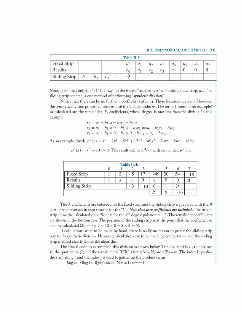
B.2. POLYNOMIAL ARITHMETIC 231
Table B.3:
Note, again, that only the “+1” (i.e., b0) on the b strip “reaches over” to multiply the a strip, a4. Thissliding strip scheme is one method of performing “synthetic division,”
Notice that there can be no further c coefficients after c4. These locations are zero. However,the synthetic division process continues until the 1 slides under a7.The terms (three, in this example)so calculated are the remainder, R, coefficients, whose degree is one less than the divisor. In thisexample
r0 = a5 − b1c4 − b2c3 − b3c2
r1 = a6 − b1 × 0 − b2c4 − b3c3 = a6 − b2c4 − b3c3
r2 = a7 − b1 × 0 − b2 × 0 − b3c4 = a7 − b3c4 .
As an example, divide A7(x) = x7 + 2x6 + 5x5 + 17x4 − 49x3 + 20x2 + 54x − 18 by
B3(x) = x3 + 10x − 3. The result will be C4(x) with remainder, R2(x).
Table B.4:
The A coefficients are entered into the fixed strip, and the sliding strip is prepared with the B
coefficients reversed in sign (except for the “1”). Note that zero coefficients are included . The resultsstrip show the calculated c coefficients for the 4th degree polynomial, C. The remainder coefficientsare shown in the bottom row. The position of the sliding strip is at the point that the coefficient r0
is to be calculated (20 + 0 × 7 − 10 × 0 − 5 × 3 = 5).If calculations were to be made by hand, there is really no reason to prefer the sliding strip
way to do synthetic division. However, calculations are to be made by computer — and the slidingstrip method clearly shows the algorithm.
The Pascal code to accomplish this division is shown below. The dividend is A, the divisor,B, the quotient is Q, and the remainder is REM. Order(A) = N, order(B) = m. The index k “pushesthe strip along,” and the index j is used to gather up the product terms:
Begin {Begin Synthetic Division----}
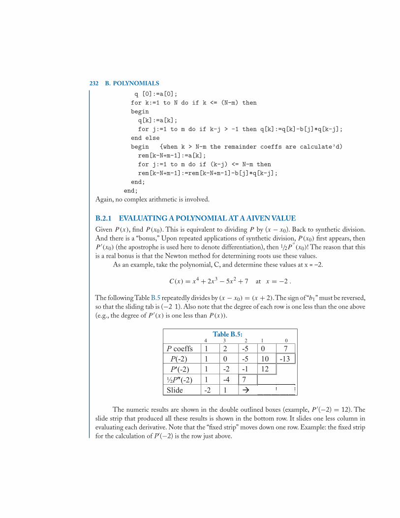
232 B. POLYNOMIALS
q [0]:=a[0];for k:=1 to N do if k <= (N-m) thenbeginq[k]:=a[k];for j:=1 to m do if k-j > -1 then q[k]:=q[k]-b[j]*q[k-j];
end elsebegin {when k > N-m the remainder coeffs are calculate’d)rem[k-N+m-1]:=a[k];for j:=1 to m do if (k-j) <= N-m thenrem[k-N+m-1]:=rem[k-N+m-1]-b[j]*q[k-j];
end;end;
Again, no complex arithmetic is involved.
B.2.1 EVALUATING A POLYNOMIAL AT A AIVEN VALUEGiven P(x), find P(x0). This is equivalent to dividing P by (x − x0). Back to synthetic division.And there is a “bonus,” Upon repeated applications of synthetic division, P(x0) first appears, thenP ′(x0) (the apostrophe is used here to denote differentiation), then 1/2P
′′(x0)! The reason that this
is a real bonus is that the Newton method for determining roots use these values.As an example, take the polynomial, C, and determine these values at x = –2.
C(x) = x4 + 2x3 − 5x2 + 7 at x = −2 .
The following Table B.5 repeatedly divides by (x − x0) = (x + 2).The sign of “b1” must be reversed,so that the sliding tab is (−2 1). Also note that the degree of each row is one less than the one above(e.g., the degree of P ′(x) is one less than P(x)).
Table B.5:
The numeric results are shown in the double outlined boxes (example, P ′(−2) = 12). Theslide strip that produced all these results is shown in the bottom row. It slides one less column inevaluating each derivative. Note that the “fixed strip” moves down one row. Example: the fixed stripfor the calculation of P′(−2) is the row just above.
B.3. EVALUATING POLYNOMIAL ROOTS 233
In the above table, the rows can be filled in simultaneously. The table can be filled columnby column, rather than row by row. This makes the computer coding all the easier. The code givenbelow takes advantage of this. The polynomial is of degree N and its coefficients are c[k]. The valueof x is given in xx.The value of the polynomial at x is in f, the derivative at x in f1, and 1/2 the secondderivative in f2. In the code, below, the polynomial coefficients are in array c[k].
Begin {Evaluate the polynomial and its derivatives at xx}f:=c [0]; f1:=c[0]; f2:=c[0];for k:=1 to N dobeginf:=c[k]+xx*f;if k < N then f1:=f+xx*f1;if k < N-1 then f2:=f1+xx*f2;
end;end;
A very simple routine. However, xx may be complex, and so the routine must be done in complexarithmetic.
B.3 EVALUATING POLYNOMIAL ROOTS
Deriving the polynomial roots from its coefficients is certainly not a simple problem. For polynomialsof degree greater than 4 there is no direct approach — only iterative methods are available. Arecommended approach is summarized as follows:
• Laguerre’s method (below) is recommended to provide an initial estimate of a root.
• When a close estimate is found (Laguerre), then Newton’s method produces excellent results.
• Using the result from Newton’s method, the original polynomial can be “deflated” by dividingthe polynomial by the newly found root factor(s), to a product of the root factor times apolynomial of lesser degree. In this way, the degree of each “stage” becomes reduced untila quadratic, cubic or quartic polynomial remains. At that point, the remaining roots can becalculated directly.
The equations for the Laguerre and Newton methods will be given here, without derivation.
B.3.1 THE LAGUERRE METHODGiven a polynomial, P(x), of degree N, and an initial estimate of a root at x0, define:
G ≡ P ′(x0)
P (x0)and H ≡ G2 − P ′′(x0)
P (x0).
234 B. POLYNOMIALS
(Note: The apostrophe is used here to denote differentiation.)
Then h = −N
G ±√(N − 1)(NH − G2)
, and the next estimate of the root is x0 + h .
B.3.2 THE NEWTON METHODWhen a root is located closely enough to ensure convergence of the Newton method:
1
h= −P ′(x0)
P (x0)+
12P ′′(x0)
P ′(x0).
Note that all the factors (P and its derivatives) are obtained directly via the above “Pascal-like”routine. Just put them together to find h. The next estimate of the root is x0 + h.
B.3.3 AN EXAMPLEAn example will provide a general overview of the methods involved:
P(x) = 1.0x5 + 2.0x4 + 3.0x3 + 4.0x2 + 5.0x + 6.0 .
Using an initial value of 0 + j0, the Laguerre method quickly finds roots near (−0.806 ± j1.223).Then Newton refines the roots to (−0.8057865 ± j1.22290471).
The deflation process reduces the polynomial to third degree (note that two roots have beenfound so that the deflation is from degree 5 to degree 3), with coefficients:
1.000000 0.388427 0.229234 2.797480
This cubic polynomial can be solved directly. However, for the example we continue the iterativemethods.
The Laguerre method works with this new polynomial to find (0.552 ± j1.253). Now, theNewton method is used — but with this difference: Newton will always use the original polynomial,because inaccuracies in the first roots will effect the accuracies of the deflated polynomial. Newtonfinds (0.551685 ± j1.2533352).
Now a polynomial x + 1.491798, whose root is obviously −1.491798. And this completes theprocess.
It should be noted that these calculations must be done with high precision. This exampleproblem was done using the “extended” variable type in Turbo Pascal (Delphi). The first root wasactually determined to be:
−8.05786469389031E − 0001 1.22290471337441E + 0000
Root evaluation is very sensitive to small changes in the coefficients. It may be that this sensitivitycan be reduced somewhat by the transformation given at the beginning of the appendix, which

B.3. EVALUATING POLYNOMIAL ROOTS 235
results in both c0 and cn being set to 1.0. For the problems used in preparing this appendix, theaccuracy was so great that the transformation appeared to make no difference. But in more realisticproblems, it might.

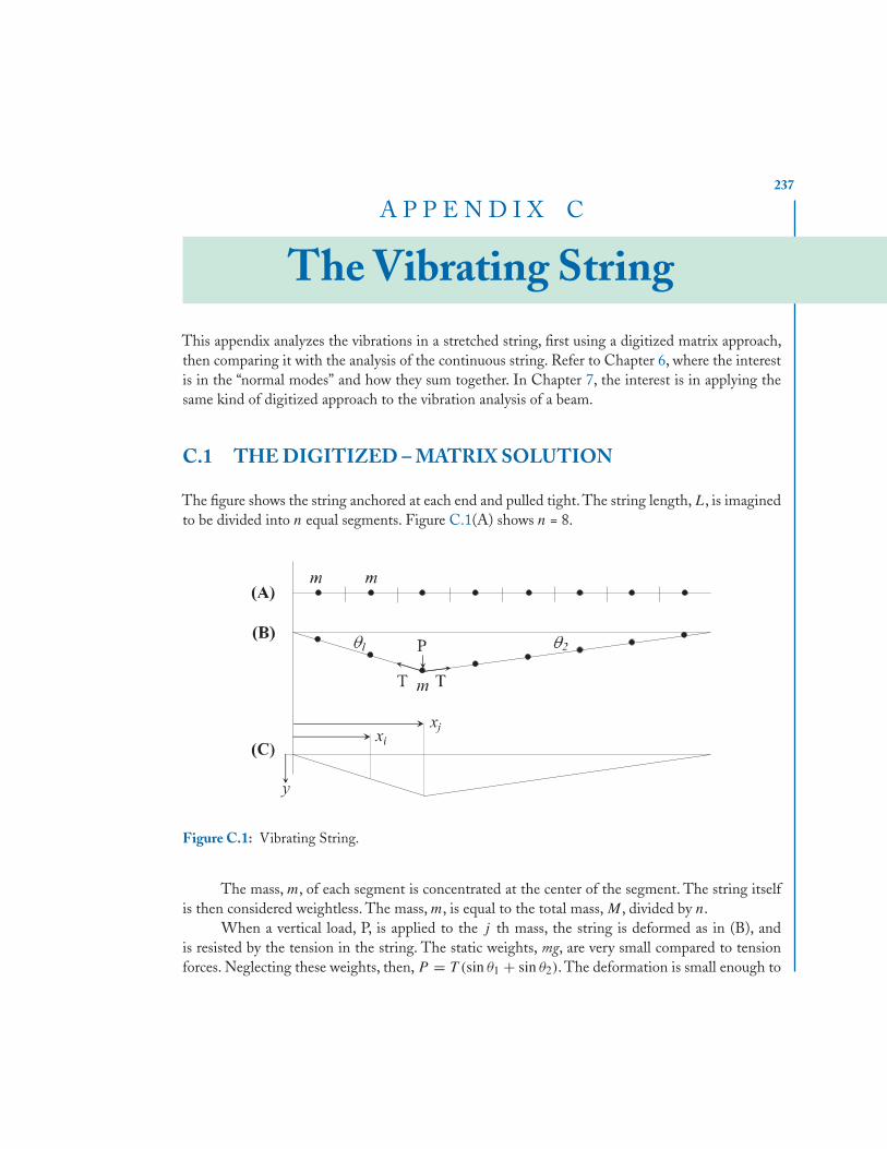
237
A P P E N D I X C
The Vibrating StringThis appendix analyzes the vibrations in a stretched string, first using a digitized matrix approach,then comparing it with the analysis of the continuous string. Refer to Chapter 6, where the interestis in the “normal modes” and how they sum together. In Chapter 7, the interest is in applying thesame kind of digitized approach to the vibration analysis of a beam.
C.1 THE DIGITIZED – MATRIX SOLUTION
The figure shows the string anchored at each end and pulled tight. The string length, L, is imaginedto be divided into n equal segments. Figure C.1(A) shows n = 8.
Figure C.1: Vibrating String.
The mass, m, of each segment is concentrated at the center of the segment. The string itselfis then considered weightless. The mass, m, is equal to the total mass, M , divided by n.
When a vertical load, P, is applied to the j th mass, the string is deformed as in (B), andis resisted by the tension in the string. The static weights, mg, are very small compared to tensionforces. Neglecting these weights, then, P = T (sin θ1 + sin θ2). The deformation is small enough to
238 C. THE VIBRATING STRING
consider sinθ = tanθ , and cosθ = 1 (note the chosen positive x and y directions, in (C)). Then
sin θ1 ≈ y(xj )
xj
and sin θ2 ≈ y(xj )
L − xj
, and
P = y(xj )T
[1
xj
+ 1
L − xj
]= T L
y(xj )
xj (L − xj ).
Then the deflection at xj due to the load, P , at xj , is
y(xj ) = Pxj (L − xj )
T L.
The diagram, (C), similar triangles, shows that, for xi < xj ,
y(xi)
y(xj )= xi
xj
⇒ y(xi) = Pxi
T L(L − xj ), for xi < xj .
For xi > xj just exchange xj and xi , ⇒ y(xi) = Pxj
T L(L − xi), for xi > xj .
This is by virtue of the “reciprocity theorem” i.e., the deflection at xi due to the load at xj isthe same as the deflection at xj due to the same load at xi . Or, just work out the geometry.
Using these equations, and setting the load, P , to unity, a dimensionless “influence matrix,”[wij ], can be defined. First, note that xk = L
n(k − 1
2 ), for k =1 ..n. Then, for xi < xj :
wij = xi
T L(L − xj ) = 1
T L
[Ln(i − 1
2 )] [
L − Ln(j − 1
2 )]
wij = L
T n2(i − 1
2 )(n − j + 12 ); dimensionless except for the
L
Tmultiplier .
The [w] matrix will be symmetric (prove it), and we should extract the L/T term as a multiplier. Now,if (vertical) loads are applied to some, or all the mass points, given as the elements of vector, p, theresultant deflection y is just y = L
TWp. For example, the displacement y1 is equal to its displacement
due to the load at j = 1, plus that at j = 2, plus … etc.If the string is vibrating freely, the loads are just the inertial forces, −miyi = −M
nyi
y(t) = −LM
TWy(t); with wij = 1
n3(i − 1
2 )(n − j + 12 ) .
Note that an additional “n” factor is absorbed into W, which has the eigenvalues, λi , and theeigenvectors, vi . Given the eigenvalue analysis of W, the solution to this vector differential equationis constructed as a linear summation of its eigenvectors (or “normal modes”):
y(t) =n∑
r=1
vr (ar cos ωrt + br sin ωrt); with ωr =√
T
LMλr
.
C.2. THE CONTINUOUS FUNCTION SOLUTION 239
The coefficients ar and br can be determined from the initial conditions by using the orthogonalityproperty of the eigenvectors: vi • vj = δij (i.e., the eigenvectors are normalized). That is, by settingt = 0, the ar coefficients are found from the initial positions of the masses, and the br coefficientsare determined from the initial velocities of the masses.
y(0) =∑
r
vrar ; Now dot through with the vector vk : ⇒ vk • y(0) =∑
r
vk • vrar
ar = vr • y(0)
y(0) =∑
r
vrωrbr ; again dot through by vk : vk • y(0) =∑
r
vk • vrωrbr , and
br = vr • y(0)
ωr
.
Summary: In this analysis, the eigenvalues determine the frequencies (in terms of length, mass,and tension) and for each of these there is a corresponding eigenvector, or normal mode. A normalmode is a spatial description of the string. A sum of these modes builds the solution along thex-dimension (the y vector). Each mode brings along a constant and sinusoidal time function. Thereare just enough initial conditions to determine the constants, since each mass point starts (time t =0) with an initial position and velocity.
The determination of the constants depends on the orthogonality of the “normal modes,”
C.2 THE CONTINUOUS FUNCTION SOLUTIONOur objective is to compare the continuous solution to the one above; therefore, its derivation willbe very brief. The highlights presented here follow the derivation in [4, p. 431].
The string is now viewed as continuous, and a solution y(x, t) is sought. As above, the initialconditions are given, say, as y0(x), and y0(x).
The governing equation for the vibration of the string is the one dimensional wave equation:
T L
M
∂2y
∂x2= ∂2y
∂t2
where T , L, and M are defined as in the matrix solution.We assume a solution of the form y(x, t) = ejωtf (x).
∂2y
∂x2= ejωtf ′′, and
∂2y
∂t2= −ω2ejωtf .
Substituting these into the wave equation, results in the ordinary differential equation:
f ′′ + Mω2
T Lf = 0, whose solution is
f (x) = c1 sin
√M
T Lωx + c2 cos
√M
T Lωx .
240 C. THE VIBRATING STRING
Since f (0) = 0, c2 must be zero. However, f (L) = 0 also, and this cannot mean that c1 = 0, elsethere would be only the trivial solution. Nevertheless
sin
√M
T LωL = sin
√ML
Tω = 0 .
This condition can be met if
√ML
Tω = nπ, or ωn =
√T
MLnπ , since sin = 0 at these values.
That is, there are an infinity of values, ωn, where n can be any integer > 0. For each of thesevalues, there are corresponding functions, fn(x) and yn(x, t)
fn(x) = c1 sinnπx
L; and yn(x, t) = c1e
jωnt sinnπx
L.
Note that both the real (cos) and imaginary (sin) parts of y(x, t) solve the wave equation, their sumis also a solution:
yn = sinnπx
L
(an cos
√T
MLnπt + bn sin
√T
MLnπt
).
And the final solution is the infinite sum of all the yn functions, y(x, t) =∞∑
n=1
yn.
At time t = 0 the initial position of the string is y0(x):
y(x, 0) = y0(x) =∑n
an sinnπx
L
and this shows clearly that the string position is a sum of sin functions, in the same way that thematrix solution string position is a sum of eigenvectors. Furthermore, a group of sin functions canform an orthogonal set — as shown in work with Fourier series. From a mathematical handbook∫ π
0sin ax sin bx dx = 0, (b �= a); and
∫ π
0sin2 ax dx = π
2.
Then with the change of variable z = Lπx, the second integral value is L
2 .
Then∫ L
0y0(x) sin
kπx
Ldx =
∑n
an
∫ L
0sin
kπx
Lsin
nπx
Ldx = L
2ak .
The coefficients bk are calculated in the same way, resulting in the final solution:
y(x, t) =∞∑
n=1
sinnπx
L
(an cos
√T
MLnπt + bn sin
√T
MLnπt
)
an = 2
L
L∫0
y0(x) sinnπx
Ldx, and bn = 2
nπL
L∫0
y0(x) sinnπx
Ldx .
C.3. EXERCISES 241
It is truly remarkable how similar the two solutions are.
C.3 EXERCISESC.1. Show that the [w] matrix is symmetric.
C.2. Show that y(t) =n∑r
arvr cos ωrt is a solution to y(t) = −LMT
Wy(t).

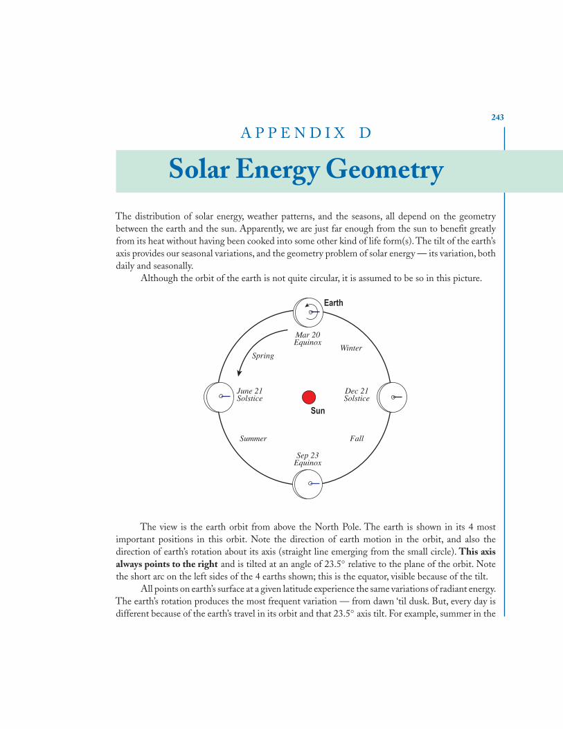
243
A P P E N D I X D
Solar Energy GeometryThe distribution of solar energy, weather patterns, and the seasons, all depend on the geometrybetween the earth and the sun. Apparently, we are just far enough from the sun to benefit greatlyfrom its heat without having been cooked into some other kind of life form(s). The tilt of the earth’saxis provides our seasonal variations, and the geometry problem of solar energy — its variation, bothdaily and seasonally.
Although the orbit of the earth is not quite circular, it is assumed to be so in this picture.
The view is the earth orbit from above the North Pole. The earth is shown in its 4 mostimportant positions in this orbit. Note the direction of earth motion in the orbit, and also thedirection of earth’s rotation about its axis (straight line emerging from the small circle). This axisalways points to the right and is tilted at an angle of 23.5◦ relative to the plane of the orbit. Notethe short arc on the left sides of the 4 earths shown; this is the equator, visible because of the tilt.
All points on earth’s surface at a given latitude experience the same variations of radiant energy.The earth’s rotation produces the most frequent variation — from dawn ‘til dusk. But, every day isdifferent because of the earth’s travel in its orbit and that 23.5◦ axis tilt. For example, summer in the
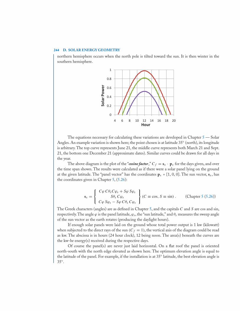
244 D. SOLAR ENERGY GEOMETRY
northern hemisphere occurs when the north pole is tilted toward the sun. It is then winter in thesouthern hemisphere.
0
0.2
0.4
0.6
0.8
1
4 6 8 10 12 14 16 18 20
Sola
r Pow
er
Hour
The equations necessary for calculating these variations are developed in Chapter 5 — SolarAngles. An example variation is shown here; the point chosen is at latitude 35◦ (north), its longitudeis arbitrary. The top curve represents June 21, the middle curve represents both March 21 and Sept.21, the bottom one December 21 (approximate dates). Similar curves could be drawn for all days inthe year.
The above diagram is the plot of the “cosine factor,” Cf = sx · px for the days given, and overthe time span shown. The results were calculated as if there were a solar panel lying on the groundat the given latitude. The “panel vector” has the coordinates px = {1, 0, 0}. The sun vector, sx , hasthe coordinates given in Chapter 5, (5.26):
sx =⎧⎨⎩
Cϕ CθsCϕs + Sϕ Sϕs
Sθs Cϕs
Cϕ Sϕs − Sϕ Cθs Cϕs
⎫⎬⎭ (C ≡ cos, S ≡ sin) . (Chapter 5 (5.26))
The Greek characters (angles) are as defined in Chapter 5, and the capitals C and S are cos and sin,respectively.The angle ϕ is the panel latitude, ϕs , the “sun latitude,” and θs measures the sweep angleof the sun vector as the earth rotates (producing the daylight hours).
If enough solar panels were laid on the ground whose total power output is 1 kw (kilowatt)when subjected to the direct rays of the sun (Cf = 1), the vertical axis of the diagram could be readas kw. The abscissa is in hours (24 hour clock), 12 being noon. The area(s) beneath the curves arethe kw-hr energy(s) received during the respective days.
Of course the panel(s) are never just laid horizontal. On a flat roof the panel is orientednorth-south with the north edge elevated as shown here. The optimum elevation angle is equal tothe latitude of the panel. For example, if the installation is at 35◦ latitude, the best elevation angle is35◦.
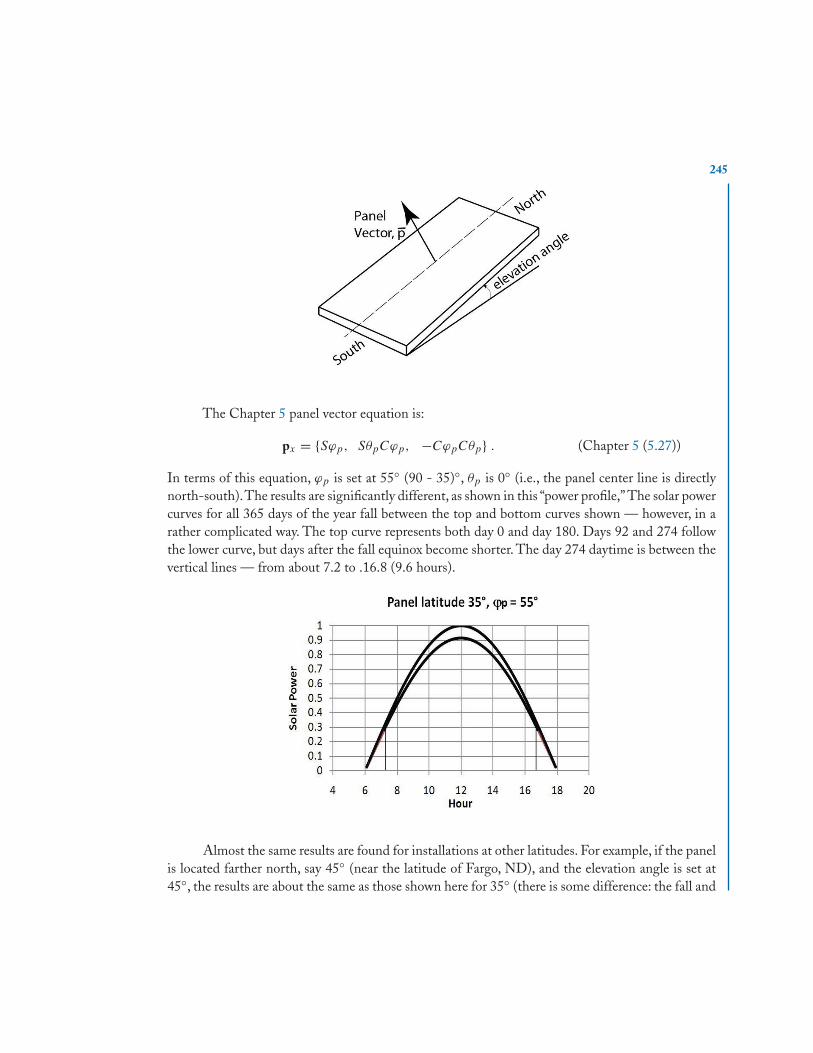
245
The Chapter 5 panel vector equation is:
px = {Sϕp, SθpCϕp, −CϕpCθp} . (Chapter 5 (5.27))
In terms of this equation, ϕp is set at 55◦ (90 - 35)◦, θp is 0◦ (i.e., the panel center line is directlynorth-south).The results are significantly different, as shown in this “power profile,” The solar powercurves for all 365 days of the year fall between the top and bottom curves shown — however, in arather complicated way. The top curve represents both day 0 and day 180. Days 92 and 274 followthe lower curve, but days after the fall equinox become shorter. The day 274 daytime is between thevertical lines — from about 7.2 to .16.8 (9.6 hours).
Almost the same results are found for installations at other latitudes. For example, if the panelis located farther north, say 45◦ (near the latitude of Fargo, ND), and the elevation angle is set at45◦, the results are about the same as those shown here for 35◦ (there is some difference: the fall and
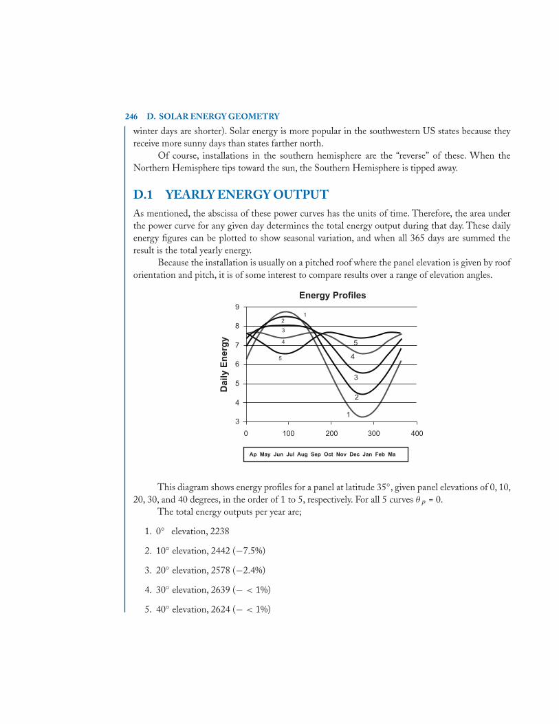
246 D. SOLAR ENERGY GEOMETRY
winter days are shorter). Solar energy is more popular in the southwestern US states because theyreceive more sunny days than states farther north.
Of course, installations in the southern hemisphere are the “reverse” of these. When theNorthern Hemisphere tips toward the sun, the Southern Hemisphere is tipped away.
D.1 YEARLY ENERGY OUTPUTAs mentioned, the abscissa of these power curves has the units of time. Therefore, the area underthe power curve for any given day determines the total energy output during that day. These dailyenergy figures can be plotted to show seasonal variation, and when all 365 days are summed theresult is the total yearly energy.
Because the installation is usually on a pitched roof where the panel elevation is given by rooforientation and pitch, it is of some interest to compare results over a range of elevation angles.
This diagram shows energy profiles for a panel at latitude 35◦, given panel elevations of 0, 10,20, 30, and 40 degrees, in the order of 1 to 5, respectively. For all 5 curves θp = 0.
The total energy outputs per year are;
1. 0◦ elevation, 2238
2. 10◦ elevation, 2442 (−7.5%)
3. 20◦ elevation, 2578 (−2.4%)
4. 30◦ elevation, 2639 (− < 1%)
5. 40◦ elevation, 2624 (− < 1%)
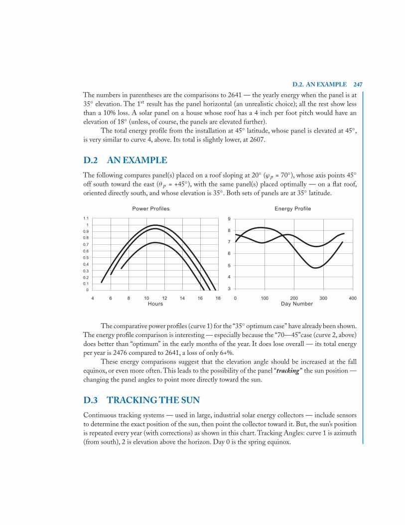
D.2. AN EXAMPLE 247
The numbers in parentheses are the comparisons to 2641 — the yearly energy when the panel is at35◦ elevation. The 1st result has the panel horizontal (an unrealistic choice); all the rest show lessthan a 10% loss. A solar panel on a house whose roof has a 4 inch per foot pitch would have anelevation of 18◦ (unless, of course, the panels are elevated further).
The total energy profile from the installation at 45◦ latitude, whose panel is elevated at 45◦,is very similar to curve 4, above. Its total is slightly lower, at 2607.
D.2 AN EXAMPLE
The following compares panel(s) placed on a roof sloping at 20◦ (ϕp = 70◦), whose axis points 45◦off south toward the east (θp = +45◦), with the same panel(s) placed optimally — on a flat roof,oriented directly south, and whose elevation is 35◦. Both sets of panels are at 35◦ latitude.
The comparative power profiles (curve 1) for the “35◦ optimum case” have already been shown.The energy profile comparison is interesting — especially because the “70—45”case (curve 2, above)does better than “optimum” in the early months of the year. It does lose overall — its total energyper year is 2476 compared to 2641, a loss of only 6+%.
These energy comparisons suggest that the elevation angle should be increased at the fallequinox, or even more often. This leads to the possibility of the panel “tracking” the sun position —changing the panel angles to point more directly toward the sun.
D.3 TRACKING THE SUN
Continuous tracking systems — used in large, industrial solar energy collectors — include sensorsto determine the exact position of the sun, then point the collector toward it. But, the sun’s positionis repeated every year (with corrections) as shown in this chart. Tracking Angles: curve 1 is azimuth(from south), 2 is elevation above the horizon. Day 0 is the spring equinox.
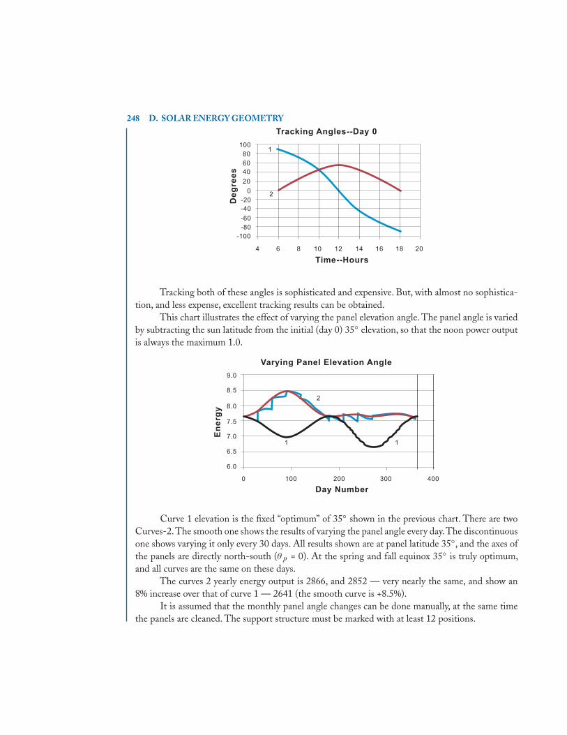
248 D. SOLAR ENERGY GEOMETRY
Tracking both of these angles is sophisticated and expensive. But, with almost no sophistica-tion, and less expense, excellent tracking results can be obtained.
This chart illustrates the effect of varying the panel elevation angle. The panel angle is variedby subtracting the sun latitude from the initial (day 0) 35◦ elevation, so that the noon power outputis always the maximum 1.0.
Curve 1 elevation is the fixed “optimum” of 35◦ shown in the previous chart. There are twoCurves-2.The smooth one shows the results of varying the panel angle every day.The discontinuousone shows varying it only every 30 days. All results shown are at panel latitude 35◦, and the axes ofthe panels are directly north-south (θp = 0). At the spring and fall equinox 35◦ is truly optimum,and all curves are the same on these days.
The curves 2 yearly energy output is 2866, and 2852 — very nearly the same, and show an8% increase over that of curve 1 — 2641 (the smooth curve is +8.5%).
It is assumed that the monthly panel angle changes can be done manually, at the same timethe panels are cleaned. The support structure must be marked with at least 12 positions.
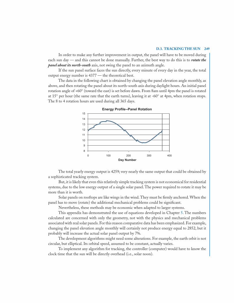
D.3. TRACKING THE SUN 249
In order to make any further improvement in output, the panel will have to be moved duringeach sun day — and this cannot be done manually. Further, the best way to do this is to rotate thepanel about its north-south axis, not swing the panel to an azimuth angle.
If the sun panel surface faces the sun directly, every minute of every day in the year, the totaloutput energy number is 4377 — the theoretical best.
The data in the following chart is obtained by changing the panel elevation angle monthly, asabove, and then rotating the panel about its north-south axis during daylight hours. An initial panelrotation angle of +60◦ (toward the east) is set before dawn. From 8am until 4pm the panel is rotatedat 15◦ per hour (the same rate that the earth turns), leaving it at -60◦ at 4pm, when rotation stops.The 8 to 4 rotation hours are used during all 365 days.
The total yearly energy output is 4259; very nearly the same output that could be obtained bya sophisticated tracking system.
But, it is likely that even this relatively simple tracking system is not economical for residentialsystems, due to the low energy output of a single solar panel. The power required to rotate it may bemore than it is worth.
Solar panels on rooftops are like wings in the wind. They must be firmly anchored. When thepanel has to move (rotate) the additional mechanical problems could be significant.
Nevertheless, these methods may be economic when adapted to larger systems.This appendix has demonstrated the use of equations developed in Chapter 5. The numbers
calculated are concerned with only the geometry, not with the physics and mechanical problemsassociated with real solar panels. For this reason comparative data has been emphasized. For example,changing the panel elevation angle monthly will certainly not produce energy equal to 2852, but itprobably will increase the actual solar panel output by 7%.
The development algorithms might need some alterations. For example, the earth orbit is notcircular, but elliptical. Its orbital speed, assumed to be constant, actually varies.
To implement any algorithm for tracking, the controller (computer) would have to know theclock time that the sun will be directly overhead (i.e., solar noon).

251
A P P E N D I X E
Answers to Selected Exercises
E.1 CHAPTER 12. There are m row vectors and n column vectors.
3. If A and B are square and conformable, BA is conformable. If A is mXn and B is nXm, BAis conformable
4. u1 · v1 = 0.32192
5. The product {v1}[u1] is a 4X4 matrix:
⎡⎢⎢⎣
15.833 7.4538 1.7180 20.9373−4.1953 −2.0197 −0.4655 −5.6731
7.3584 3.5424 0.8165 9.9504−10.3222 −4.9692 −1.14534 −13.9582
⎤⎥⎥⎦
6. c = x1a1 + x2a2 + · · · + xnan
7. v = {0, 0, 0}. u = [ 21, 6, 3 ]
8. It is more efficient in all cases to calculate vectors. For example, in determining ABCv multiplyCv first. In (2) v1u1v2u2, calculate the dot product u1v2 first
14. T1T2 =⎡⎣ cos θ cos ϕ − sin θ cos θ sin ϕ
sin θ cos ϕ cos θ sin θ sin ϕ
− sin ϕ 0 cos ϕ
⎤⎦, and note that the product of orthogonal ma-
trices is always orthogonal. That is: T1T2(T′2T′
1) = I
17. The transformation matrix is formed by replacing the 3,1 element (a zero) of a unit matrix by
the ratio −a31
a11.
E.2 CHAPTER 21. 5741326, s = 13; 35421, s = 8; 123465, s = 1; 654321, s = 15
2. b44b12b31b23 = b12b23b31b44 s = 2, plus c43c22c14c51c35, s = 9, minus
252 E. ANSWERS TO SELECTED EXERCISES
3. |A| = 9; |B| = −14
7. The rank of A1 is 1. It has just one independent vector.
11. The rank of A2 is 2.
13. Each factor of the expansion of the 3X3 will have 3 terms. They can all be arranged intocolumn order. Now, just differentiate. The result will be three expansions in exactly the formto be shown.
E.3 CHAPTER 3
1. Q =⎡⎣ 1 0 0
−3 1 0−2 0 1
⎤⎦, whose determinant = 1;
|A| = 2; QA =⎡⎣ 1 3 −1
0 2 40 0 1
⎤⎦ ; Qc =
⎧⎨⎩
40
−1
⎫⎬⎭
2. From QAx = Qc, x3 = −1, x2 = 2, and then x1 = −3, solved in that order.
3. In this book, complex matrices are often written with imaginary parts above the reals. Theinverse is written here in this notation. Note also, the double bars (instead of bracket), denotinga matrix.
A−1 =
∥∥∥∥∥∥∥∥∥∥∥∥∥∥∥∥∥
8.00 −2.00 −3.007.00 6.00 −2.00
6.00 −1.00 −2.005.00 6.00 −2.00
−3.00 −1.00 1.000.00 − − 2.00 0.00
∥∥∥∥∥∥∥∥∥∥∥∥∥∥∥∥∥5. Given Ax = c, and B = A−1, if two columns of A are interchanged, corresponding rows of
both B and x will be interchanged. Compare the following to problems 1 & 2, above:
Given Ax = c, with A =⎡⎣ 3 1 −1
11 3 16 2 −1
⎤⎦, then A−1 =
⎡⎣ 2.5 0.5 −2
−8.5 −1.5 7−2 0 1
⎤⎦ ,
E.4. CHAPTER 4 253
and x =⎧⎨⎩
2−3−1
⎫⎬⎭
E.4 CHAPTER 42. a2 × a3 = −{3, 6, 1}; a2 × a3 • a1 = −14; a2 × a3 • c = −4. Then x1 = 2/
7
4. The rank of M is just 2
5(a). Neither the columns nor the rows of M are independent.
5(c). Since the rank is 2, then x3, x4, and x5 can be chosen arbitrarily, and
{x1
x2
}={
1373
}x3 −
{2323
}x4 −
{5323
}x5
5(d). Given Mx = y, the set will be compatible iff y is orthogonal to {-1, 2, 1}.
6(a). The columns of A are independent.
6(b). The rows of A are dependent.
6(c). z = {–14, –1, 20, 39, 1} is orthogonal to the columns of M.
6(d). x = {–3, 1, 2, –1}
6(e). With the given y vector the set is incompatible.
12. Begin with the X matrix shown at right. The desired determinant is obtained by striking outrow 2 and column 2 of X. However, this determinant is just the minor of the 2,2 element inX. |X| = (x4 − x3)(x4 − x2)(x4 − x2)(x3 − x2)(x3 − x1)(x2 − x1)
X =
⎡⎢⎢⎢⎢⎣
1 x1 x21 x3
1
1 x2 x22 x3
2
1 x3 x23 x3
3
1 x4 x24 x3
4
⎤⎥⎥⎥⎥⎦
In the text discussing Lagrange polynomials it is shown that XA = I, that is, the two matricesare inverses. Then the minor of the x22 element is a22 multiplied by |X|.
a22 = x1x3 + x1x4 + x3x4
(x2 − x1)(x2 − x3)(x2 − x4)
|X|a22 is equal to the determinant of the reduced matrix given in the exercise.
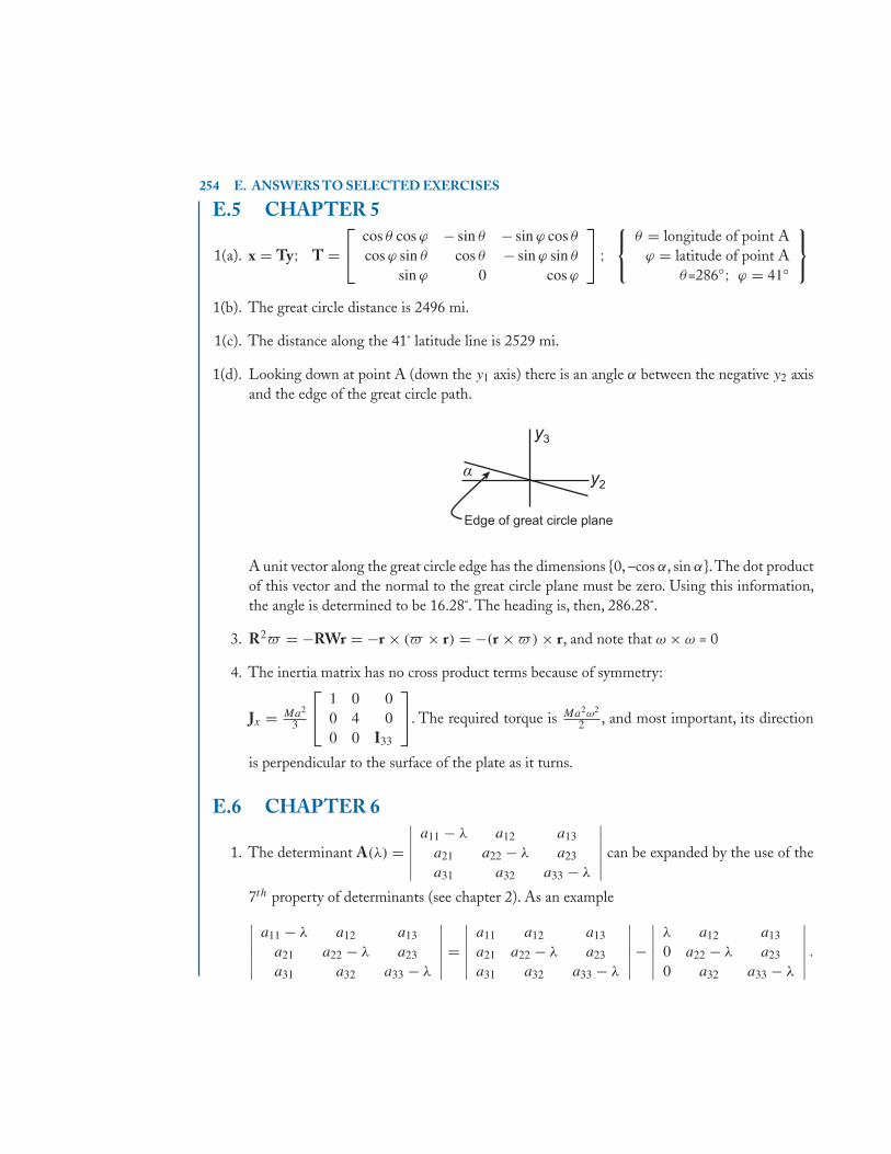
254 E. ANSWERS TO SELECTED EXERCISES
E.5 CHAPTER 5
1(a). x = Ty; T =⎡⎣ cos θ cos ϕ − sin θ − sin ϕ cos θ
cos ϕ sin θ cos θ − sin ϕ sin θ
sin ϕ 0 cos ϕ
⎤⎦ ;
⎧⎨⎩
θ = longitude of point Aϕ = latitude of point A
θ=286◦; ϕ = 41◦
⎫⎬⎭
1(b). The great circle distance is 2496 mi.
1(c). The distance along the 41˚ latitude line is 2529 mi.
1(d). Looking down at point A (down the y1 axis) there is an angle α between the negative y2 axisand the edge of the great circle path.
A unit vector along the great circle edge has the dimensions {0, –cos α, sin α}.The dot productof this vector and the normal to the great circle plane must be zero. Using this information,the angle is determined to be 16.28˚. The heading is, then, 286.28˚.
3. R2� = −RWr = −r × (� × r) = −(r × �) × r, and note that ω × ω = 0
4. The inertia matrix has no cross product terms because of symmetry:
Jx = Ma2
3
⎡⎣ 1 0 0
0 4 00 0 I33
⎤⎦. The required torque is Ma2ω2
2 , and most important, its direction
is perpendicular to the surface of the plate as it turns.
E.6 CHAPTER 6
1. The determinant A(λ) =∣∣∣∣∣∣
a11 − λ a12 a13
a21 a22 − λ a23
a31 a32 a33 − λ
∣∣∣∣∣∣ can be expanded by the use of the
7th property of determinants (see chapter 2). As an example
∣∣∣∣∣∣a11 − λ a12 a13
a21 a22 − λ a23
a31 a32 a33 − λ
∣∣∣∣∣∣ =∣∣∣∣∣∣
a11 a12 a13
a21 a22 − λ a23
a31 a32 a33 − λ
∣∣∣∣∣∣−∣∣∣∣∣∣
λ a12 a13
0 a22 − λ a23
0 a32 a33 − λ
∣∣∣∣∣∣ .
E.6. CHAPTER 6 255
With continued use of this property, the following results are obtained:
∣∣A(λ)∣∣ = c0λ
3 + c1λ2 + c2λ + c3
c0 = −1c1 = a11 + a22 + a33
c2 = −∣∣∣∣ a11 a13
a31 a33
∣∣∣∣−∣∣∣∣ a11 a12
a21 a22
∣∣∣∣−∣∣∣∣ a22 a23
a32 a33
∣∣∣∣c3 = ∣∣A∣∣
This expansion is easier than it appears, and can be generalized to work for characteristicdeterminants of higher order.
2. Using the above expansion, the characteristic polynomial for the given matrix is:
P(λ) = c0λ3 + c1λ
2 + c2λ + c3 = −λ3 + 4λ2 + 7λ − 10 = λ3 − 4λ2 − 7λ + 10= (λ − 1)(λ + 2)(λ − 5)
The adjoint of [A – I] is [A + 2I][A – 5I] = A2 – 3A – 10I =
⎡⎣ 72 12 24
72 −12 −24−216 36 72
⎤⎦ which
yields the two vectors v1 = {1, −1, 3} and u1 = [ 6, 1, -2 ], and note that u1•v1 = 1.
In the same manner, the other two vector pairs are determined such that:
U =⎡⎣ 6 −1 −2
3 0 −11 1 0
⎤⎦ ; V =
⎡⎣ 1 −2 1
−1 2 03 −7 3
⎤⎦, normalized such that UV = VU = I
4. B =⎡⎣ 18 −1 −6
−18 1 660 −3 −20
⎤⎦, and |B(λ)| = λ3 + λ2 − 2λ = 0 = λ(λ − 1)(λ + 2).
Note that the third eigenvalue is zero (and B is singular). However,
adj{B(λ = 0)} = −2
⎡⎣ 1 1 0
0 0 03 3 0
⎤⎦, which yields the same eigenvectors that were found for
the original A matrix.
5. The (symmetric) A matrix has the eigenvalues, 1 and 4. Its eigenvectors are V =1√2
[1 1
−1 1
]
256 E. ANSWERS TO SELECTED EXERCISES
The square root matrix will have the same eigenvectors as A. When this matrix is multipliedby itself the result is V t�VV t�V = V t�2V . Therefore, the square root matrix must be:
1
2
[1 1
−1 1
] [2 00 1
] [1 −11 1
]= 1
2
[3 −1
−1 3
].
6. The characteristic equation of[ −0.7 2
−0.6 1.5
]is λ2 − 0.8λ + 0.15 = (λ − 0.3)(λ − 0.5)
Adj{A(λ=0.3)} =Aa(.3) = [A − 0.5I] =[ −1.2 2
−0.6 1
];Adj{A(λ=0.5)} = [A − 0.3I] =[ −1 2
−0.6 1.2
]
Z1(λ1 = .3) = [A − 0.3I](0.3 − 0.5)
=[
6 −103 −5
]; Z2(λ2 = .5) = [A − 0.5I]
(0.5 − 0.3)=[ −5 10
−3 6
]
Sin(A) = sin(λ1)Z1 + sin(λ2)Z2 =[ −0.624006 1.839053
−0.551716 1.398952
]
six decimals are given in the event that you would like to show that sin 2(A) + cos 2(A) = I.
7(a). The solution includes the diagonal matrix [δij1
λj −λ] which insists that there is no solution for
λ = λj .
7(c). Yet, when the c vector is orthogonal to the j th normal mode (as in this case), the termλ − λj does not appear in the solution; thus, a solution exists at that critical e-value.Though mathematically correct, it would be very dangerous to depend on this, physically.
9. A reduces to the P matrix
⎡⎣ 16 −66 54
1 0 00 1 0
⎤⎦ which yields the required coefficients. The
column vectors are the same as the row vectors, since the given matrix is symmetric.
The roots are 1.08352, 9.86399, and 5.05249
Also used in this calculation are the following S and S−1 matrices:
S =⎡⎣ 1
9 −1 19 1 2
30 − 1
3 1 13
0 0 1
⎤⎦ ; S−1 =
⎡⎣ 9 −30 25
0 −3 40 0 1
⎤⎦
Note that the matrix product [S][S−1] = I.
E.7. CHAPTER 7 257
E.7 CHAPTER 7Problems 2 & 3. With x1 and x2 measured from fixed locations, the equations of motion of bothare Mx + Kx = df cos ωt where:
M =[
m1 00 m2
]; K =
[k1 + k2 −k2
−k2 k2
]; A = M−1K =
[k1+k2
m1
−k2m1
−k2m2
k2m2
]
2. In this case, m1 = m2 and k1 = k2, and there is no driving force. Now, set ω =√
km
and
[Iλ − A] =[
λ − 2ω2 ω2
ω2 λ − ω2
]; Det =λ2 − 3ω2λ + ω4; Then λ = 3 ± √
5
2ω2
And the 2 resonant frequencies (rad/sec), are 0.618ω and 1.618ω.
3. This time, the k and m values are not the same, and there is a driving force as shown above. Inthis equation we assume a solution x = acosωt.This reduces the above equation to an algebraicone by which we can solve for the maximum amplitudes (a1 and a2) of x1 and x2.
−ω2Ma + Ka = f ; where f = {f0, 0}a = [K − ω2M]−1f
[K − ω2M] =[
k1 + k2 − ω2m1 −k2
−k2 k2 − ω2m2
]
Set D equal to the determinant of [K - ω2M]. Then:
a = 1D
[k2 − ω2m2 k2
k2 k1 + k2 − ω2m1
]{f0
0
}
Note that if the ratio of k2 divided by m2 is made equal to ω2, the term k2 − ω2m2 goes tozero. In both problems 2 and 3, the mass, m1 will be motionless, if m1 is driven at the resonantfrequency of the single mass/spring system—unless the determinant also goes to zero. Does it?
5. The matrices are: (It is easier to work with the inverse of M)
M−1 =⎡⎣ 38.64 0.0 0.0
0.0 12.88 0.00.0 0.0 12.88
⎤⎦ ; K =
⎡⎣ 10 −5 −5
−5 15 0−5 0 15
⎤⎦ ;
C =⎡⎣ 0.6 −0.3 −0.3
−0.3 0.8 0−0.3 0 0.8
⎤⎦
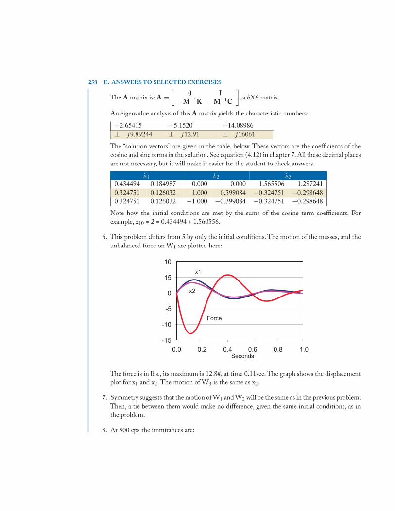
258 E. ANSWERS TO SELECTED EXERCISES
The A matrix is: A =[
0 I−M−1K −M−1C
], a 6X6 matrix.
An eigenvalue analysis of this A matrix yields the characteristic numbers:
−2.65415 −5.1520 −14.08986± j9.89244 ± j12.91 ± j16061
The “solution vectors” are given in the table, below. These vectors are the coefficients of thecosine and sine terms in the solution. See equation (4.12) in chapter 7. All these decimal placesare not necessary, but it will make it easier for the student to check answers.
λ1 λ2 λ3
0.434494 0.184987 0.000 0.000 1.565506 1.2872410.324751 0.126032 1.000 0.399084 −0.324751 −0.2986480.324751 0.126032 −1.000 −0.399084 −0.324751 −0.298648
Note how the initial conditions are met by the sums of the cosine term coefficients. Forexample, x10 = 2 = 0.434494 + 1.560556.
6. This problem differs from 5 by only the initial conditions. The motion of the masses, and theunbalanced force on W1 are plotted here:
The force is in lbs., its maximum is 12.8#, at time 0.11sec. The graph shows the displacementplot for x1 and x2. The motion of W3 is the same as x2.
7. Symmetry suggests that the motion of W1 and W2 will be the same as in the previous problem.Then, a tie between them would make no difference, given the same initial conditions, as inthe problem.
8. At 500 cps the immitances are:
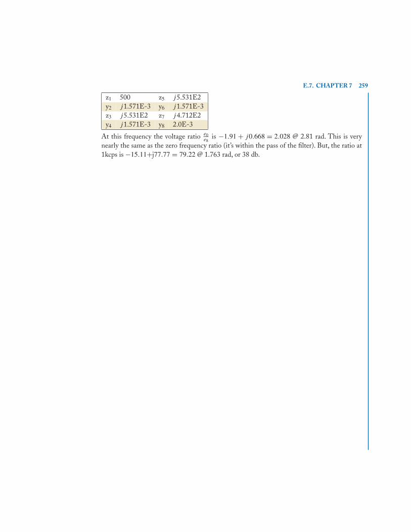
E.7. CHAPTER 7 259
z1 500 z5 j5.531E2y2 j1.571E-3 y6 j1.571E-3z3 j5.531E2 z7 j4.712E2y4 j1.571E-3 y8 2.0E-3
At this frequency the voltage ratio e0e8
is −1.91 + j0.668 = 2.028 @ 2.81 rad. This is verynearly the same as the zero frequency ratio (it’s within the pass of the filter). But, the ratio at1kcps is −15.11+j77.77 = 79.22 @ 1.763 rad, or 38 db.


261
Bibliography
[1] Hildebrand, F. B., Methods of Applied Mathematics. Prentice-Hall, Englewood Cliffs, NewJersey, 1958.Chapter 1 of this book is an excellent introduction to: “Matrices, Determinants, and LinearEquations.”
[2] Frazer, R. A., Duncan, W. J., Collar, M.A., Elementary Matrices, and Some Applications toDynamics and Differential Equations. Cambridge Press.This is a very complete treatise,very concise. It isn’t all that “elementary.” Whatever the question,the answer is probably in this book.
[3] Lanczos, C., Applied Analysis. Prentice-Hall, Englewood Cliffs, New Jersey, 1958. 160A wonderful writer and “explainer.” My favorite.
[4] Pipes, L. A., Applied Mathematics for Engineers and Physicists. McGraw-Hill Book Co., 1958.166, 239
[5] Pipes, L. A., Matrix Methods for Engineering. Prentice-Hall, Englewood Cliffs, New Jersey,1963.Both of these books are gems. Matrix Methods is a must for any engineer.
[6] Wylie, C. R., Advanced Engineering Mathematics. McGraw Hill, 1960.A fine undergraduate book, written by a great teacher at University of Utah.
[7] Faddeeva, V. N., Computational Methods of Linear Algebra. Dover Publications, Inc. New York.This reference has influenced this book through the notes of a dear friend and boss, Dr. Lee.I. Wilkinson at the General Electric Co., and later, Honeywell. The method of Danilevskydescribed herein follows Lee’s notes — which references this book.
[8] Press,W., Flannery, B.,Teukolsky, S, and Vetterling,W. Numerical Recipes in Pascal. CambridgeUniversity Press, 1989.Laguerre’s method for determining the initial estimate of a polynomial root, described inAppendix B, was taken from this book, page 296.This reference describes Crout’s method, which is more efficient in the solution of simultaneousequations than that found in this work.


263
Author’s Biography
MARVIN J. TOBIASA native Utahn (Salt Lake), Marvin J. Tobias graduated in Mechanical Engineering (ME) fromthe University of Utah.
He joined the General Electric Company and began a series of rotating assignments throughvarious Departments in the East, initially in the General Engineering Laboratory, then in the Jet En-gine Department. In the fall, Marv successfully applied for a three year intensive training program—the Advanced Engineering Program. During the latter years of the program his assignments werein radar signal and data processing.
Assignments in both ME and EE proved the need for further education and training inmathematics, so the middle year (B course—applied mathematics) was particularly interesting.
Over the years, Marv became a lecturer for the B course, developing many notes on matrixalgebra and calculus. As the PC became more powerful, with sophisticated word processing andgraphics software, those notes became the content of this book.

265
Index
Adjoint matrix, 35adjoint and inverse, 45in Cramer’s rule, 50of characteristic equation, 146, 160
Algebraic equations, 1Analysis of Ladder networks, 214Angular Momentum, 133Angular rotation, 123Angular velocity matrix, 126Augmented matrix, 59–62, 68, 69, 71
Backward substitution, 63, 65, 67–70code, 70
Characteristic determinant, 51Characteristic equation, 146Characteristic matrix, 145
adjoint of, 149inverse of, 158
Characteristic polynomial, 146Characteristic values, see eigenvaluesCombinations, 38, 40Computer graphics, 120Conservative system
example, 191sinusoidal response, 197transient response, 191, 196
Coordinate transforms, 108earth centered coordinates, 109
Cramer’s rule, 24, 50, 215Cumulant, the, 214
Decoupled equations, 158, 194, 204Defective matrix, 157Del operator, the, 95Determinant, 2
cofactors, 37complex determinant, 51Cramer’s Rule, 24, 50definition, 23, 25evaluation, 46
complex pivot, 46Gaussian reduction, 47pivotal condensation, 46rlist, clist, 48
expansion, 23expansion by lower order minors, 38expansion by minors, 33
first minors, 33geometric concepts, 41inversions of indices, 27LaPlace expansion, 33, 35minors and cofactors, 33of matrix product, 41permutation of indices, 26properties of, 30rank less than n, 50rank of, 32
Differential equations: reduced to 1st order,201, 202
Direction cosine, 84Double pendulum, 188Dynamical matrix, 191
266 INDEX
Dynamics of a particle, 127acceleration, 129, 130velocity, 128
Dynamics of a rigid body, 130angular momentum, 133examples, 138inertia matrix, 134moment of momentum, 133rotation, 132spinning top, 135torque equation, 137translation, 131
Eigenvalue analysisDanilevsky’s method, 171example, 148, 168geometry of, 152non-symmetric matrix, 148, 168of similar matrices, 171symmetric matrices, 151
Eigenvalue problemdefinition of, 145in vibrating systems, 183
Eigenvalues, 146in complex conjugate pairs, 203matrix with a double root, 156of symmetric matrices, 151
Eigenvectors, 146direction, 147normal modes, 159normalized, 147orthogonality, 157row, column, 147
Energy method, see Lagrange’s equationsEquations of motion, 185
conservative system, 186non-conservative system, 185, 186
Eulerian rotations, 115
Forward substitution, 68, 69, 71–73code, 70
Gauss reduction, 47, 61code, 62example, 66method, 47, 62pivoting, 62, 64, 66, 67rlist, clist, 64
Gauss-Jordan reduction, 59, 87, 93pivoting in, 59, 60singular matrices, 61
Inertiamoment of inertia, 135product of inertia, 135
Initial value problem solution, 191Interpolation, 100Inversion
of a complex matrix, 78of a triangular matrix, 75of diagonal matrix, 58
Kirchhoff ’s Laws, 188Kronecker delta, 189
Lagrange interpolation polynomials, 100Lagrange’s equations, 184, 185Law of sines, 132Linear equation sets, 55, 83
as vector transform, 83compatibility, 91, 92geometry of, 88least squares solutions, 94non unique solution, 90overdetermined, 93square, n = m, 88underdetermined, 91vector solution, 89
Linear independence: of vector set, 85–86
INDEX 267
Linear regression, 96equations for, 98example, 98
LU decomposition, 68example, 70pivoting in, 68, 69
Matrixadjoint and inverse, 44adjoint rank, 45definition of, 1dimensions, 1, 2
Matrix algebra, 3addition, subtraction, 4conformability, 4conformable, 7multiplication, 6multiplication by a scalar, 4non-commutative, 8of complex matrices, 18partitioning, 7vector multiplication, 4
Matrix differentiation, 123Matrix inversion, 55
by orthogonalization, 77by partitioning, 71
example, 79computer operations in, 72diagonalization, 57elementary operations, 55Gauss reduction, 61
algorithm, 63partial pivoting, 68pivoting, 62
Gauss-Jordan reduction, 59improving the inverse, 74LU decomposition, 68
example, 70of a complex matrix, 78
of a triangular matrix, 75of diagonal matrix, 58singular matrices, 61
Matrix partitioning, 7, 14in matrix multiplication, 14
Matrix polynomial, 122Matrix transforms, 121
of matrix product, 122of matrix sum, 122of the inverse matrix, 122of the transpose matrix, 122
Matrix types, 9adjoint matrix, 38, 44complex matrix, 11diagonal matrix, 9inverse matrix, 11orthogonal matrix, 9skew-symmetric matrix, 10symmetric matrix, 10triangular matrix, 10unit matrix, 9
Mechanical/electrical analogues, 186
n Dimensional space, 84Newton’s Laws, 185Nonconservative system, 201
example problem, 203initial problem solution, 203, 207sinusoidal response, 207, 211sinusoidal response example, 210
Normal modes, 197Notation, 2
matrix, 3vector, 2, 84
Orthogonalmatrix, 105transform, 105vectors, 84, 88
268 INDEX
Orthonormal, 105
Partial pivoting, see Gauss reductionPartitioning, see Matrix partitioningPivot, see Gauss reductionPolar coordinates, 111Polynomial arithmetic, 229
finding roots of, 233deflation, 233Laguerre method, 234Newton method, 234
generation from roots, 227value at a point, 232
Polynomials, see Appendix B
Quadratic form, 152, 186Differentiation of, 223
Rankof matrix, 92of vector set, 86
Rayleigh’s dissipation function, 186Reciprocity, 200Reduced matrix, 148References, 261Right hand rule, 107
positive angle, 107rlist, clist, 64Runge-Kutta integration, 216
Simpson’s rule, 216
Similar matrices, 121Similarity transforms, see Matrix transformsSimultaneous equation sets, see Linear
equation setsSolar Angles, 116
sun latitude, 118, 119sun panel vector, 119, 120sun vector, 117
Solar energy geometry, see Appendix Dsolar cosine factor, 117, 244
Steady state sinusoidal response, 211example, 213
Submatrix, see Matrix partitioningSynthesis of a matrix, 147
Trace of a matrix, 149Transform matrices, 13Transposition, 8
of inverse, 12of product, 8
Unit vectors, 107
Vectorcolumn, and row, 3cross product, 17dimensionality, 84dot product, 5row, 3unit vector, 83
Vector sets, 83fill a space, 85linear independence, 85transposed set, 83
Vibrating string, 159see Appendix C
Vibrating systems, 183decoupled equations, 194, 204setting up equations, 186
Vibration of conservative systems, 185, 189equations of motion, 186, 190
Vibration problemdifferential equations of, 185
Vibrations in a continuous medium, 199vibrating beam, 199vibrating string, 159