Bank Failures and the Cost of Systemic Risk:

Evidence from 1900-1930*

Paul H. Kupiec and

Carlos D. Ramireza

Revised:

March 2010

Keywords: bank failures; credit channel; systemic risk; financial accelerator, vector autoregressions; Panic of 1907; non-bank commercial failures JEL Classification Codes: N11, N21, E44, E32 * The views and opinions expressed here are those of the authors and do not necessarily reflect those of the Federal Deposit Insurance Corporation. We are grateful to Mark Flannery, Ed Kane, Thomas Philippon, Peter Praet, Lee Davidson, Vivian Hwa, and Daniel Parivisini for helpful comments and suggestions. Ramirez acknowledges financial support from the FDIC’s Center for Financial Research. a Carlos Ramirez is Associate Professor, Department of Economics, George Mason University, and Visiting Fellow, Center for Financial Research, FDIC. Email: cramire2@gmu.edu. Paul Kupiec is an economist at the FDIC. Email: pkupiec@fdic.gov.

- 2 -

Bank Failures and the Cost of Systemic Risk: Evidence from 1900-1930

Abstract:

This paper investigates the effect of bank failures on economic growth using new data on bank failures from 1900 to 1930. The sample period predates active government stabilization policies and includes several severe banking crises. We use VAR and difference-in-difference methods to estimate the impact of bank failures on economic activity. VAR results show bank failures have negative and long-lasting effects on economic growth. Three quarters after a bank failure shock involving one percent of total bank liabilities (primarily deposits), GNP is reduced by about 6.9 percent. Difference-in-difference results suggest that bank failures trigger an increase in non-bank failures. The evidence supports the hypothesis that bank failures reduce economic growth and provides a lower bound estimate of the cost of banking sector systemic risk. Keywords: bank failures; credit channel; systemic risk; financial accelerator, vector autoregressions; Panic of 1907; non-bank commercial failures JEL Classification Codes: N11, N21, E44, E32

- 3 -

I. Introduction

The link between bank failures and economic growth continues to be an important

topic in macroeconomics.1 Economists and policy makers have long been interested in

quantifying the degree to which bank failures create negative externalities that reduce

economic growth. If these externalities are economically important, they are a

manifestation of financial sector systemic risk.

Banks are a source of systemic risk if the social cost of a bank failure exceeds the

direct losses of failing bank financial claimholders. One component of this social cost is

the subsequent loss in output associated with bank failures.2 The failure of any firm may

create externalities and losses in output, but because of banks importance in the

intermediation process, the costs and externalities associated with a bank failure are

likely to be much larger than those associated with the failure of a non-bank entity.

The credit channel literature on monetary policy [Bernanke and Gertler (1989,

1990, 1995), Bernanke and Blinder (1992)] emphasizes the link between banks’ cost of

capital and the borrowing costs and final demands of bank-dependent borrowers. If a

credit channel is operative under normal monetary conditions, should important banks

fail, the externality on bank-dependent borrowers is likely to be substantial.

A number of studies including Hogart, Reis and Saporta (2002) [HRS], Boyd,

Kwak and Smith (2005) [BKS], Gupta (2005), and Krosner, Laeven and Klingebiel

(2007) and Dell'Ariccia, Detragiache, and Rajan (2008) have used cross-country data on

1 Relevant citations as well as a brief overview of this literature are provided in Section II further below. 2 Recent papers on bank systemic risk focus on the strength of correlation among bank defaults and mechanisms that can propagate shocks among banks or other financial institutions. Kaufman and Scott (2003) and Schwartz (2008) provide overviews of the literature. A common feature of all discussions of systemic risk is the existence of a mechanism whereby losses to one financial institution create losses for many other financial institutions. Few of these models directly address the real economic consequences of systemic risk.

- 4 -

modern banking crises to estimate the loss in output associated with systemic banking

crisis. These studies find that banking crisis are associated reductions in the finial

demands of bank dependent borrowers and substantial losses in GDP. Cumulative loss

estimates for GDP range from 11.5 [HRS] percent of pre-crisis GDP to as high as

possibly 300 percent [BKS]. These estimates are specialized in that they focus on a

sample of catastrophic banking crisis many of which are linked with currency crisis.

There is no consensus regarding the reduction in lost output that can expected in the wake

of an increase in bank failures.3

Outside of these cross-country studies on banking crisis, the modern literature on

bank failures and economic activity is focused on two periods: the Great Depression

(1930–1933) and the U.S. savings and loan and banking crises of the late 1980s and early

1990s (S&L crisis). There is consensus that a breakdown in the banking system

intensified the Great Depression in the U.S., but Depression-era evidence from other

countries as well as evidence from the S&L crisis is ambiguous. For example, the

Canadian experience during the Great Depression does not suggest that there are large

negative externalities associated with bank failures (Haubrich, 1990; White, 1984).

Analysis of data from the S&L crisis has also produced conflicting results (see, inter alia,

Ashcraft, 2005; Alton, Gilbert, and Kochin, 1989; or Clair and O’Driscoll, 1994).

This paper investigates the effect of bank failures on economic activity using new

data on bank failures that occurred between 1900 and 1930. There are at least two

reasons why this sample period is likely to yield new insights. First, prior to the

3 It is worth pointing out that the costs we are referring to in this paper are the consequences of systemic bank failures on economic growth, not the fiscal costs of associated with the resolution of failed institutions or the costs associated with the implementation of new regulation aimed at preventing further failures. For an estimate of these costs see Honohan and Laeven (2003) and Claessens, Klingebiel, and Laeven (2003).

- 5 -

enactment of federal deposit insurance legislation in 1933, the United States experienced

repeated banking panics, some of which occurred when economic conditions were

quiescent. While many banks failed or temporarily suspended redemptions during

banking panics, many of the banks that failed during the panics were not insolvent

because of deteriorating macro-economic conditions.4 If banking crises include a banking

sector shock that is independent of shocks to the real economy then we can better identify

the linkage between the health of the banking sector and subsequent economic growth.

Second, as we document in more detail below, during this period there were no federal

government institutions or policies implemented to counteract the effects of bank failures

and exert a stabilizing influence on the economy. These two important characteristics of

this sample period allow us to use new data on banking system distress to identify new

estimates of the economic costs of bank failures.

In the analysis that follows, we use vector autoregression analysis (VAR) to

estimate the effect of bank failures on both the growth rate of industrial production and

aggregate output growth. The severity of bank failures is measured using newly

complied data on the share of banking system liabilities (predominantly deposits) in

failed banks and trusts including all state- and nationally-chartered institutions. We argue

that the data are consistent with the hypothesis that bank failures create negative

4 We argue that banking panics represent shocks to the health of the banking system are independent of contemporaneous shocks to economic growth during this period. Our assumption that banking crisis are in part generated by a banking sector shock that is independent of economic fundamentals is not above dispute. For example, Gorton (1988) argues that the banking panics during National Banking Era (1865-1914) can be explained by the rational responses of depositors reacting to new economic information that alters risk perceptions, whereas banking panics over the period 1914-1934 are more severe than can be predicted based on changing economic fundamentals alone. Calomiris and Mason (1997) [CM] analyze bank failures during the 1932 banking panic and reach a different conclusion. CM find that failed banks were financially weak and would likely have failed under non-panic conditions as well. Carlson (2008) takes issue with the CM analysis and concludes that there is a high probability that many of the banks that failed in 1932 would have been acquired, merged or recapitalized in a non-panic period.

- 6 -

externalities if: (i) an increase in bank failures on average reduces subsequent economic

growth; and, (ii) on average, poor economic growth is not followed by a higher incidence

of bank failures. We use Granger causality tests and establish that an increase in the

liabilities of failed banks, other things equal, reduces industrial production and economic

growth, but a decline in economic growth or industrial production does not lead to an

increase in failed-bank liabilities.

Our estimates suggest that, over the period 1900–1930, the variation in failed-

bank liabilities explains about 5 percent of the volatility in output growth. In addition,

we find that, all else constant, a one standard deviation innovation (14.5 basis points) in

the share of liabilities in failed banks results in a cumulative 2.4 percent decline in

industrial production (IP) growth and a cumulative 1 percent decline in GNP growth over

the following three quarters.5 The results also suggest that the effects of bank failures are

long-lasting: even after 10 quarters the cumulative decline in both IP growth and GNP

growth following the shock is still approximately 1 percent. A direct implication of these

results is that, the failure of an important financial institution (or institutions), in the

absence of intervention, is likely to have protracted macroeconomic effects.6

We provide additional evidence on the link between bank failures and economic

growth by comparing the failure rates among non-bank firms in New York and

Connecticut following the Panic of 1907. A year prior to the panic, business conditions in

New York and Connecticut were similar to business conditions in the rest of the country

and neither state had banking sector problems. 1907 brought important financial

5 To put the magnitude of the shock into perspective, as of 2009 Q4, 14 U.S. banks held 1 percent or greater share of domestic U.S. deposits. 6 Hogart, Reis, and Saporta (2002), Boyd , Kwak and Smith (2005) and Anari, Kolari, and Mason (2005) also find long lasting effects associated with bank failures. We elaborate on this result in Section IV further below.

- 7 -

institution failures in New York, but none in Connecticut. Non-bank firm failures spiked

in New York following the onset of the banking panic and non-bank failures remained

elevated for another two quarters. In contrast, non-bank business failures in Connecticut

remained stable throughout the period. When economic performance is measured by time

series data on the liabilities of non-financial commercial enterprise failures in each state,

a formal difference-in-difference analysis supports the hypothesis that bank failures cause

and increase in non-bank commercial failures. We interpret this evidence as further

support for the hypothesis that bank failures depress economic growth.

Taken together, our findings suggest that bank failures create significant negative

externalities that reduce economic growth. The estimate of the loss in aggregate output is

a lower bound estimate of the cost of systemic risk in the banking sector as it excludes

the direct deposit, equity and credit losses associated with bank failures. Our findings

predate active government policies aimed at mitigating the negative economic effects of

bank failures—policies such as uniform standards for prudential bank supervision,

federal deposit insurance, and efficient bank resolution policies. These policies may have

helped to attenuate the negative costs associated with a bank failure, but they also may

have promoted moral hazard and increased bank risk taking. Whether or not these

policies have on balance reduced the negative externalities associated with banking sector

distress is an open issue. 7

This paper is only one of many that investigate the extent to which bank failures

amplify economic distress. Section II reviews the contributions of several earlier studies.

Subsequent sections discuss the importance of the sample period (Section III); the

7 Poorly designed government policies may alter bank risk taking incentives and create additional social costs not present in our sample period. See for example, Demirguc-Kunt and Kane (2002) and Kaufman and Scott (2003).

- 8 -

macroeconomic data, the VAR model, and the empirical results (Section IV); and the

difference-in-difference analysis of New York and Connecticut during the Panic of 1907

(Section V). Section VI concludes.

II. Research on Bank Failures and Economic Activity: A Brief Overview8

Economists have studied the link between bank failures and subsequent economic

growth for well over a century. Jevons (1884) speculates that volatility in sunspot

activity affects climate, creating volatility in the agricultural and commodity prices,

which in turn affects banks and the economy. Jevons’s theory does not emphasize the

importance of banks in the economic growth process and, as far as we know, it has not

been tested.

In the aftermath of the Panic of 1907, a number of studies investigated aspects of

banking sector stability as a prelude to new legislation and banking system reforms.

Sprague (1910) studies bank failures and banking panics in the United States and finds

that international gold outflows cause, simultaneously, bank failures and a decline in

economic activity. Kemmerer (1910) finds that seasonal changes in the demand for

money, stemming from changes in agricultural sector borrowing, explain the joint

variation of stock prices, commercial failures, and banking panics between 1890 and

1908.

Friedman and Schwartz (1963) (FS) study the U.S. Great Depression and find that

bank failures triggered a loss of public confidence in the banking system leading

consumers to hold more currency and fewer bank deposits which reduced the money

8 The literature on this issue is large and our selected review highlights only the key issues in the literature.

- 9 -

multiplier and the money supply. Because the decline in the money supply was not offset

by monetary policy, nominal economic activity declined.9

Bernanke (1983) extends the FS analysis to incorporate the effect of bank failures

on investment spending. In Bernanke’s bank-centered model of business finance, firms

depend on bank lending for investment and working capital funding. Firms typically have

a long-term relationship with a single bank and when the bank fails, the relationship is

dissolved and the information gained through the relationship is lost. When firms seek

funding from new bankers, they face increased costs while they establish the new

banking relationship. Thus, for some period after a bank failure, investments by bank-

dependent firms are discouraged by increased funding costs and investments may be

limited by the availability of internal funds.10

Bank failures can also have secondary effects on the lending behavior of

surviving banks (Bernanke, 1983). Heightened uncertainty regarding deposit redemptions

induces surviving banks to increase their reserves by reducing loans to bank-dependent

businesses. Unable to tap external capital markets, businesses are forced to reduce

investment spending which results in a magnified reduction in GDP through the Keynes

(1936) investment multiplier.

Other studies confirm the importance of the bank-dependent borrower channel.

Calomiris and Mason (2003) focus on local banking markets and find that a significant

portion of the decline in economic activity from 1930 to 1932 is explained by reduced

9 FS argue that the banking failures of the Great Depression era could have been avoided, or at least mitigated, if the Federal Reserve System had been more generous in providing discount window lending to troubled banks, which would have given solvent banks access to liquidity without changing their need to hold currency reserves thereby stabilizing the money supply. 10 For more evidence on how bank affiliations facilitated access to capital markets in the pre-Depression era, see Ramirez (1999) and Calomiris and Hubbard (1995).

- 10 -

bank loan supply which reduced investment spending. Anari, Kolari, and Mason (2005)

use VAR methods to investigate the relationship between the liquidation of failed banks

and the depth and duration of the Great Depression. They find that bank failures have a

long-lasting negative effect on economic activity partly because bank failures restrict

access to the deposits in failed institutions. During this period, depositors at failed banks

were precluded from accessing their funds for an extended time, and when their accounts

became liquid, depositors generally faced sizable losses.11 The loss in depositors’

liquidity resulted in reduced consumption and investment spending.

In contrast to the U.S. experience, the experience of other countries during the

Great Depression is not consistent with strong bank failure externalities. Haubrich (1990)

studies the Great Depression in Canada using Bernanke’s methodology. During the

depression, Canada experienced a monetary contraction and a decline in output almost as

dramatic as the one in the United States. Unlike the U.S., Canada did not experience a

single bank failure during its Great Depression era notwithstanding the fact that there was

no central bank in Canada until 1935.12 While there were no Canadian bank failures in

the Great Depression, the number of bank branches in Canada did decline by about 10

percent. Still, Haubrich finds no measurable effect of branch closures on Canadian GDP.

11 Goldenweiser et al. (1932) estimate that between 1921 and 1930 the deposit recovery rate was 55.7 percent (table 25, page 195). Although this figure does not cover the Depression period, it illustrates the gravity of the situation before the establishment of federal deposit insurance. 12 The source of the Canadian system’s resilience remains in dispute but some scholars have attributed it to the diversification benefits from branch banking (FS 1963; Bordo, 1986; Ely, 1988; O’Driscoll, 1988); the effective lender of last resort function provided by the Canadian Bankers Association (CBA) (Bordo, 1986); and the existence of a 100 percent implicit government guarantee on deposits (Kryazanowski and Roberts, 1993). These explanations are, however, not beyond dispute. For example, Carr, Matherson and Quigley (1995) argue that the CBA did not arrange mergers for insolvent institutions nor were depositors protected by a government guarantee (or a perception thereof) as some faced losses when banks were suspended.

- 11 -

Many countries in Central and Eastern Europe also experienced banking crisis

during the Great Depression era.13 Similar to Canada, the United Kingdom,

Czechoslovakia, Denmark, Lithuania, the Netherlands and Sweden experienced

depression conditions without breakdowns in their banking systems (Grossman, 1994).

The literature hypothesizes factors that may have provided stability to these national

banking systems during the Great Depression, but to our knowledge, existing studies

have not analyzed whether banking system distress magnified real sector weakness.14

Banking scholars also reach conflicting conclusions when studying data from the

U.S. S&L crisis period. For example, Ashcraft (2005) investigates FDIC-induced

closures of 38 subsidiaries of First Republic Bank Corporation in 1988 and 18

subsidiaries of First City Bank Corporation in 1992. He concludes that, as a result of the

closures, real income declined by about 3 percent in areas served by these banks. In

contrast, Alton, Gilbert and Kochin (1989), using county-level data from Kansas,

Nebraska, and Oklahoma over the period 1981–1986, do not find any significant

relationship between bank failures and measures of local economic activity. Clair and

O'Driscoll (1994) use Gilbert and Kochin's methodology to study the impact of bank

failures on local economic activity in several Texas counties between 1981 and 1991.

Like Gilbert and Kochin, they do not find any significant relationship.

The results of studies based on data from the S&L crisis period are not directly

comparable to the results derived from Great Depression era data. During the S&L crisis

13 Grossman (1994) identifies a banking crisis if any one of the following occurs: (1) a large proportion of a country’s bank’s fail; (2) a large important bank fails; or (3) or extraordinary government intervention prevents (1) or (2) from occurring. Using this definition, the Great Depression was associated with banking crisis in Switzerland, Yugoslavia, France, Belgium, Latvia, Hungary, Poland, Estonia, Romania, Germany, Italy and Norway in addition to the United States. 14 This gap in the literature likely reflects the fact that few countries have high quality measures of aggregate economic activity available for this historical period.

- 12 -

period, both the Federal Reserve and banking regulators took actions to attenuate the

economic impacts of banking system distress. Bank failures were delayed (relative to

what would have happened in the Great Depression) as weak institutions continued

funding themselves with insured deposits which reduced the risk of a bank run. While

legislative inaction ensured that resource constraints slowed the supervisory resolution

process, undercapitalized depository institutions continued to fund lending activity.15

Deposit insurance quelled the public’s demand for precautionary currency holdings while

the Federal Reserve discount window was available to provide liquidity to solvent banks

which mitigated their need to call in loans. The Federal Reserve also pursued a monetary

policy designed to offset problems in depository institutions.16 All of these factors likely

helped to offset any negative effects of bank failures on economic growth.

Among existing studies, Grossman (1993) is the most closely related to our study.

Using data on the fraction of national banks that failed during the National Banking Era

(1863–1914), Grossman (1993) estimates a structural IS-LM model that includes the

effects of bank failures. His estimates suggest that a “small” shock in bank failures can

erase 8 percentage points of GDP growth, whereas a “large” shock in bank failures can

reduce the GNP growth rate by 26 percentage points. Grossman notes that these

estimated magnitudes are large, but he argues that they are reasonable when compared to

the historical record.

Grossman analyzes the effects of the number of national bank failures. Over the

period he examined (1863-1914), roughly a third of banking system assets were held by

state-chartered institutions and in many years, state-chartered banks outnumbered

15 See for example Kane (1989), or Romer and Weingast (1991). 16 See for example Clouse (1994), or Mussa (1994).

- 13 -

national banks (White 1983, pp.12-13). Importantly, in some periods, banking distress

was concentrated in the state-chartered institutions that are excluded from Grossman’s

study.17 The Grossman study, moreover, does not account for the size of failed

institutions. The importance of the negative externality generated by a bank failure

should be related to the size of a bank as institution size is a proxy for the number (and

size) of valuable relationships with bank-dependent borrowers as well as indicator of the

bank’s importance in providing transactions services.18 Large banks also are more likely

to have correspondent banking relationships which were particularly important during

this era. The failure of a key correspondent bank can have wide-ranging affects on the

reserves and lending capacity of many smaller state-chartered institutions (White pp. 68-

9).

III. The Importance of the Sample Period

During the period 1900-1930, the United States experienced three major banking

crises: one in May of 1901, another one in October of 1907, and one during the early

1920s. In addition, it endured eight minor crises.19 Many of the banking crises were not

preceded by large negative shocks to economic activity. Moreover, during this period, no

federal government policies were used to stimulate the economy, counteract recessions,

or offset the negative economic impacts of bank failures. We use a simple econometric

17 An important example is the Banking Panic of 1907. Measured by the failure rate among national banks, the 1907 Banking Panic was a mild event as the crisis was concentrated in state-chartered depository institutions. Calomiris and Gorton (1991, p. 150) identify only six national bank failures during this episode while Wicker (2000, p. 87) reports that 17 state-chartered trusts and 18 state-chartered banks either failed or suspended redemptions as a result of the crisis. Wicker, moreover, estimates that the trust failures accounted for 57 percent of the liabilities of all institutions that failed during this period. 18 Wicker (2000, p. 85) also notes the number of failed institutions is unlikely to be an accurate measure of banking system distress and the size of failed institutions must matter as well. Wicker, however, does not systematically exploit this observation. 19 Calomiris and Gorton (1991), p. 114; Miron (1986), p. 131; Kremmerer (1910), pp. 222-223.

- 14 -

model to help illustrate why these two data features enhance our ability to identify the

economic cost of bank failures.20

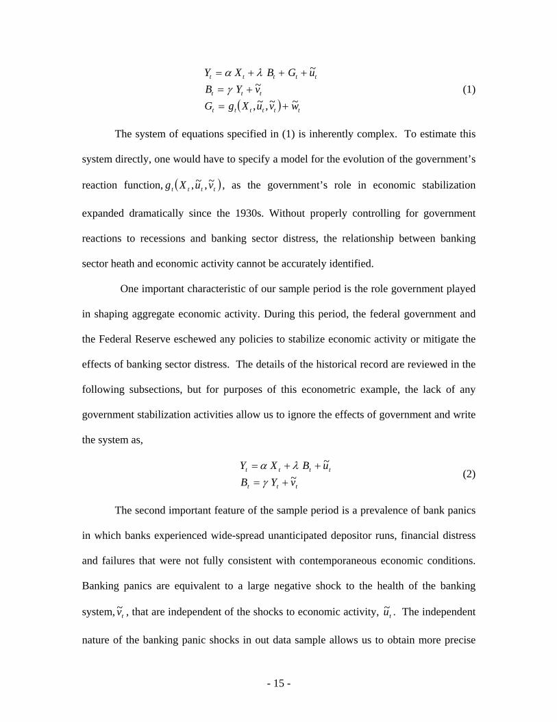
Consider a simplified model in which the health of the banking system affects

economic activity, and economic activity also affects the health of the banking system.

Let tY and tB represent, respectively, economic activity and banking system health at

time t . Let tG represent the government contribution to economic activity. tG captures

the effects of monetary, fiscal, and banking regulatory and resolution policies. Let tX (a

vector) represent all other factors which are assumed to be exogenous or predetermined

in this example and tu~ , tv~ and tw~ represent, respectively, shocks to economic activity

tu~ , the health of the banking sector tv~ , and government activity, .~tw In most

circumstances, these shocks will be correlated.

Beginning in the 1930s, government began introducing policies that were

designed to offset direct shocks to economic activity as well as negative shocks to the

health of the banking sector. The government reaction function has undergone many

changes since the 1930s. As the public and their elected officials became more

comfortable with a government role in aggregate demand management, countercyclical

fiscal and monetary policies became an important feature of the macroeconomic

environment and regulatory measures were undertaken to mitigate the economic impacts

of bank failures. To capture these time dependent effects, we write the government

reaction function as tttt vuXg ~,~, . Using these definitions, we can model the relationship

between economic activity, exogenous factors, banking sector health, and government

responses as,

20 We are indebted to Thomas Philippon for suggesting that we include this discussion.

- 15 -

tttttt

ttt

ttttt

wvuXgG

vYB

uGBXY

~~,~,

~

~

(1)

The system of equations specified in (1) is inherently complex. To estimate this

system directly, one would have to specify a model for the evolution of the government’s

reaction function, tttt vuXg ~,~, , as the government’s role in economic stabilization

expanded dramatically since the 1930s. Without properly controlling for government

reactions to recessions and banking sector distress, the relationship between banking

sector heath and economic activity cannot be accurately identified.

One important characteristic of our sample period is the role government played

in shaping aggregate economic activity. During this period, the federal government and

the Federal Reserve eschewed any policies to stabilize economic activity or mitigate the

effects of banking sector distress. The details of the historical record are reviewed in the

following subsections, but for purposes of this econometric example, the lack of any

government stabilization activities allow us to ignore the effects of government and write

the system as,

ttt

tttt

vYB

uBXY~

~

(2)

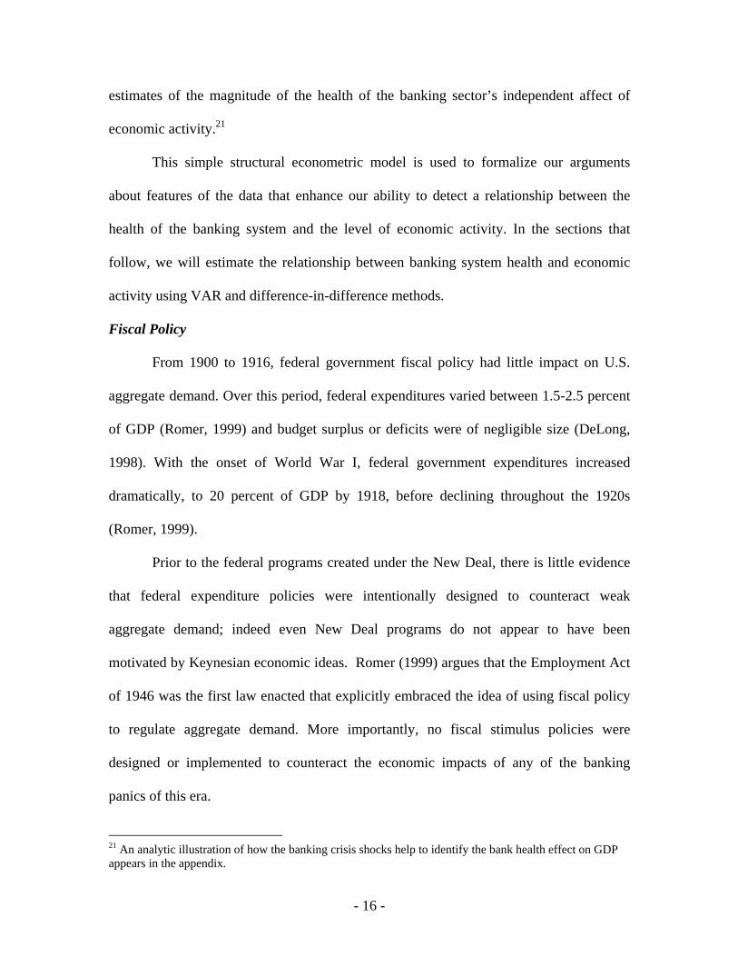
The second important feature of the sample period is a prevalence of bank panics

in which banks experienced wide-spread unanticipated depositor runs, financial distress

and failures that were not fully consistent with contemporaneous economic conditions.

Banking panics are equivalent to a large negative shock to the health of the banking

system, tv~ , that are independent of the shocks to economic activity, tu~ . The independent

nature of the banking panic shocks in out data sample allows us to obtain more precise

- 16 -

estimates of the magnitude of the health of the banking sector’s independent affect of

economic activity.21

This simple structural econometric model is used to formalize our arguments

about features of the data that enhance our ability to detect a relationship between the

health of the banking system and the level of economic activity. In the sections that

follow, we will estimate the relationship between banking system health and economic

activity using VAR and difference-in-difference methods.

Fiscal Policy

From 1900 to 1916, federal government fiscal policy had little impact on U.S.

aggregate demand. Over this period, federal expenditures varied between 1.5-2.5 percent

of GDP (Romer, 1999) and budget surplus or deficits were of negligible size (DeLong,

1998). With the onset of World War I, federal government expenditures increased

dramatically, to 20 percent of GDP by 1918, before declining throughout the 1920s

(Romer, 1999).

Prior to the federal programs created under the New Deal, there is little evidence

that federal expenditure policies were intentionally designed to counteract weak

aggregate demand; indeed even New Deal programs do not appear to have been

motivated by Keynesian economic ideas. Romer (1999) argues that the Employment Act

of 1946 was the first law enacted that explicitly embraced the idea of using fiscal policy

to regulate aggregate demand. More importantly, no fiscal stimulus policies were

designed or implemented to counteract the economic impacts of any of the banking

panics of this era.

21 An analytic illustration of how the banking crisis shocks help to identify the bank health effect on GDP appears in the appendix.

- 17 -

Monetary Policy

The Federal Reserve System, created in 1913, was established to smooth regional

credit cycles associated primarily with agricultural borrowing demands.22 Miron (1986)

argues that Federal Reserve policies were successful in dampening the seasonal variation

of nominal interest rates which reduced the frequency of banking panics.

Notwithstanding its impact on the seasonal agricultural cycle, early Federal Reserve

policies did not include an explicit counter-cyclical (business cycle) role for monetary

policy (White, 1983, p.115 ff).

In practice, the earliest coordinated Federal Reserve policies were dictated by the

U.S. Treasury’s desire to finance World War I on favorable terms. Under pressure from

Treasury, the Federal Reserve abandoned the “real bills” doctrine and allowed member

banks to discount Treasury certificates issued to finance the war at rates below those on

the Treasury certificates (Meltzer, 2003, pp. 84-90). This discounting policy created

monetary expansion and inflation. It was not until late 1919 that the Federal Reserve

System banks were permitted to raise discount rates and penalize excessive borrowing.23

A severe recession followed with widespread unemployment, declines in industrial

production and substantial deflation.24 The wholesale price index fell from 100 in 1920,

to 62.8 in 1923.

Federal Reserve operating policies were modified following the 1920-22

recession, but as late as 1924, few officials in the Federal Reserve System believed that

22 The Federal Reserve did not begin operations until 1914. Throughout the early years, Federal Reserve officials believed that monetary policy should follow a “real bills” doctrine focused on discounting commercial paper at penalty rates and providing lender of last resort facilities when needed. 23 Following WWI, several regional Federal Reserve Banks had attempted to raise discount rates but were prohibited from doing so by the Federal Reserve Board (see Meltzer 2003). 24 The severity of this recession has been in part attributed to a failure of Federal Reserve policy (Meltzer, 2003, p. 120-ff).

- 18 -

open market operations should be used to attenuate recessions (White, 1983, p.122).

Throughout the remainder of the 1920s, Federal Reserve policies were guided by three

perceived goals: (1) to re-establish the pre-World War I gold standard as the international

system of exchange; (2) to maintain price stability and avoid repeating the events of

1920-22; and, (3) to curb the growth of speculative credit (i.e., credit used to purchase

securities).25 The Federal Reserve did not embrace countercyclical monetary policies and

indeed the system could not effectively coordinate monetary policy until after the

Banking Act (1935) established the Federal Open Market Committee to coordinate

operations among the reserve banks (Meltzer, 2003, p.5).

IV. Granger Causality Evidence

Data

A vector autoregressive model (VAR) is used to estimate the linkages between

bank failures and subsequent economic growth. The VAR model includes the share of

liabilities in failed institutions (SLFI), a measure of aggregate economic activity, and two

additional economic series that are used to control for non-bank failure related shocks to

aggregate economic activity: an estimate of the inflation rate, and an estimate of the

prevailing risk premium in credit markets. The data sources for the variables used in the

VAR analysis are listed in Table A of the appendix. We discuss the characteristics of

each data series in the remainder of this section.

We use two measures of banking system distress. Our primary measure, SLFI, is

constructed from data on the liabilities (primarily deposits) of failed depository

institutions as reported in issues of Dun’s Review. These data include nearly 6,000

25 See for example, the discussions in Costigoliola (1977) or Meltzer (2003).

- 19 -

quarterly observations for the 48 states from the first quarter of 1900 through the second

quarter of 1931.26 State figures are aggregated to produce national data for each quarter.

The data include failed national banks as well as failed state-chartered banks and trust

companies.27 The failed depository liability series is normalized by total deposits as

reported in Flood (1998).28

We also construct an estimate of the time series of the failure rate of depository

institutions. The bank failure rate series is constructed from data on bank depository

institution failures as reported in Dun’s Review and the quarterly estimates of the number

of banking institutions from data reported in Historical Statistics of the United States

(1975).29

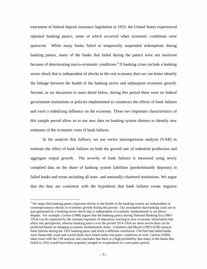
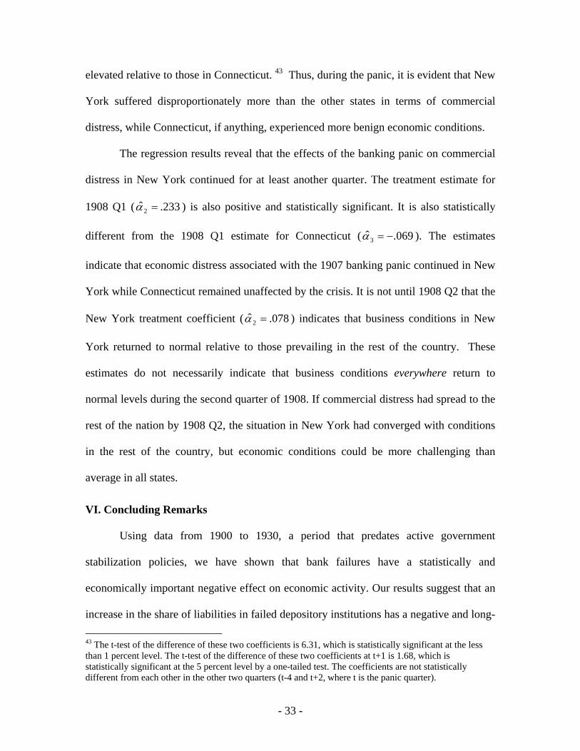
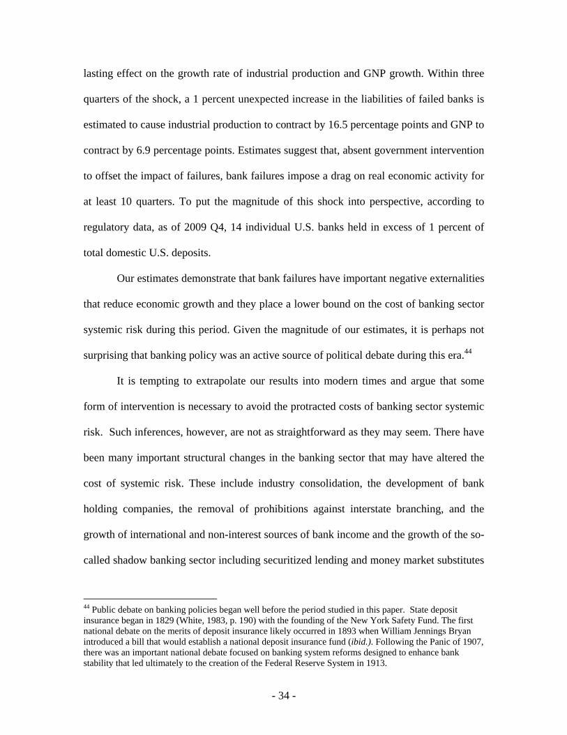
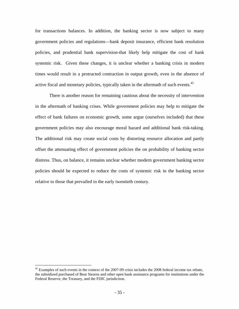
Exhibit 1 shows the depository institution failure-rate series and the SLFI series

on an annualized basis. The bank failure-rate series measures the proportion of depository

institutions that were closed, either temporarily or permanently, between 1900 and 1930.

Exhibit 1 also includes estimates of the recessionary periods (shaded bars) as identified

by Romer (1999).

The two deposit institution failure series, plotted in Exhibit 1 suggest a

significantly different record of banking system distress. The bank failure rate series is

strongly procyclical with increases in the recessions of 1900, 1903, 1907, 1910, 1920, 26 Dun’s Review reports failure data beginning in 1895, but there are periods in the 1800s when the data are unreported. From 1900, the data are reported regularly for each quarter. Dun’s Review stopped reporting these data after the second quarter of 1931. The original data are corrected for typographical errors. 27 Dun’s Review does not clarify whether bank suspensions are included in bank failures. Compared to the aggregate number of U.S. bank failures reported by Goldenweiser (1933, table 1), our numbers are marginally higher than Goldenweiser’s before 1921 but smaller thereafter. Because the Goldenweiser data excludes national bank suspensions before 1921 (and includes them thereafter), the comparison suggests that our data may include a few (but not all) suspensions. This feature of the data is unlikely have any significant effect on our results since the largest proportion of bank suspensions occurred after 1931 (Calomiris and Mason, 2003). 28 The primary source for the data reported in Flood is All Bank Statistics. The denominator in our measure is a quarterly estimate of total liabilities interpolated from annual figures. 29 Again, the denominator is a quarterly estimate interpolated from annual figures.

- 20 -

1924, and 1929. It reaches a local peak at the end or shortly following most of the

recessions in the sample period.30 In contrast, the SLFI series declines during the

recessions of 1900, 1903, 1907, 1910, 1915, and 1927. It also has local peaks

immediately prior to or very early into the recessions of 1900, 1907, 1910 and 1923.

Exhibit 1 shows that the failure rate and SLFI series diverge in the early 1900s when

failures were dominated by larger institutions and in the 1920s, when smaller institutions

failed at a relatively higher rate.

The bank failure rate series is a misleading indicator of banking sector health in at

least two important periods in the sample. Bank failure rate data suggests that banking

conditions were comparable during the 1903–1904 and 1907-1908 recessions, whereas

the SLFI data clearly identifies the severity of the banking panic of 1907. The 1907 panic

involved the failure or temporary suspension of only a few large money-center

institutions, but these failures accounted for about 1.5 percent of all system deposits.31

This level of banking system distress was not exceeded until the Great Depression. The

bank failure rate series also overstates the degree of stress in the banking system over the

period 1922–1929. Although a large number of banks failed during this period, the failed

institutions were relatively small.

It is well-known that measures of aggregate economic activity over the period

1900-1930 are imperfect (e.g., Romer, 1999) and alternative measures of aggregate

output differ as to their historical volatility characteristics. We focus on two measures of

aggregate economic activity, the Miron and Romer (1990) industrial production series

and the Balke-Gordon (1986) estimates of real GNP.

30 This pattern is clearly evident in 7 of the 9 recessions in the chart. 31 The institutions included Knickerbocker Trust, Hamilton Bank, International Trust Company, and United Exchange Bank.

- 21 -

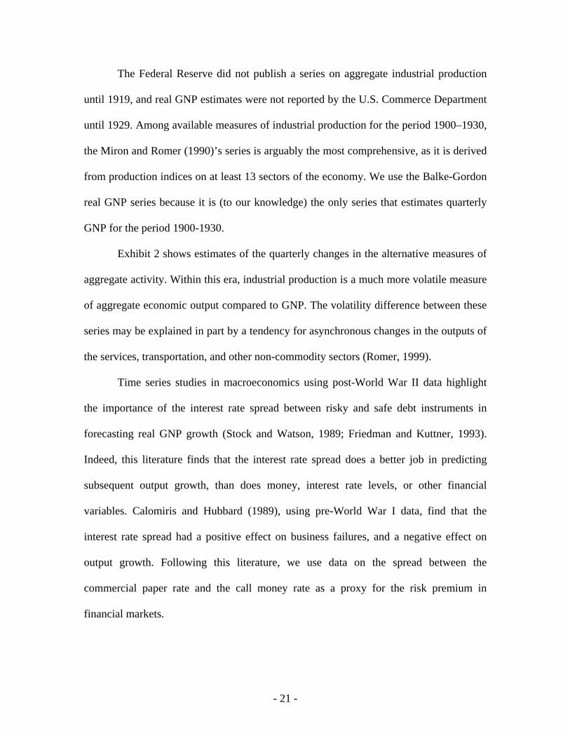
The Federal Reserve did not publish a series on aggregate industrial production

until 1919, and real GNP estimates were not reported by the U.S. Commerce Department

until 1929. Among available measures of industrial production for the period 1900–1930,

the Miron and Romer (1990)’s series is arguably the most comprehensive, as it is derived

from production indices on at least 13 sectors of the economy. We use the Balke-Gordon

real GNP series because it is (to our knowledge) the only series that estimates quarterly

GNP for the period 1900-1930.

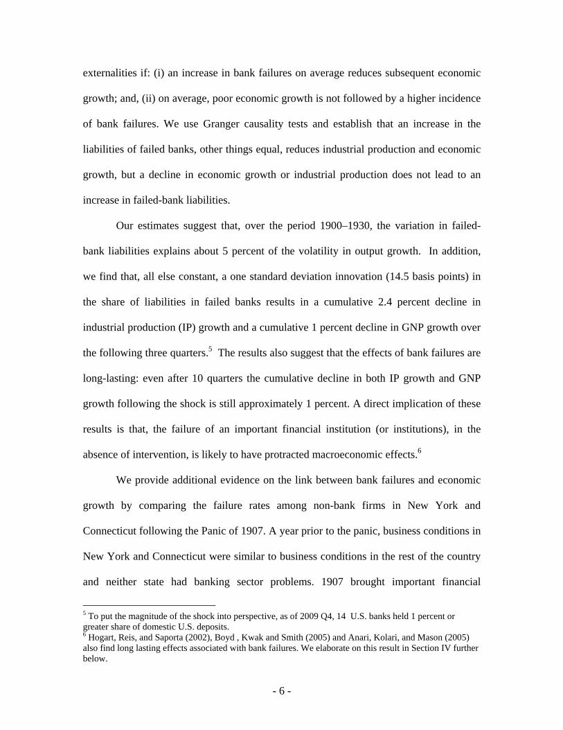
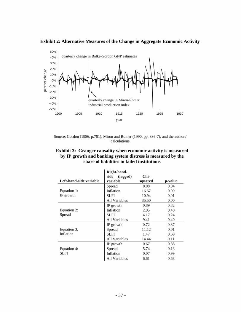
Exhibit 2 shows estimates of the quarterly changes in the alternative measures of

aggregate activity. Within this era, industrial production is a much more volatile measure

of aggregate economic output compared to GNP. The volatility difference between these

series may be explained in part by a tendency for asynchronous changes in the outputs of

the services, transportation, and other non-commodity sectors (Romer, 1999).

Time series studies in macroeconomics using post-World War II data highlight

the importance of the interest rate spread between risky and safe debt instruments in

forecasting real GNP growth (Stock and Watson, 1989; Friedman and Kuttner, 1993).

Indeed, this literature finds that the interest rate spread does a better job in predicting

subsequent output growth, than does money, interest rate levels, or other financial

variables. Calomiris and Hubbard (1989), using pre-World War I data, find that the

interest rate spread had a positive effect on business failures, and a negative effect on

output growth. Following this literature, we use data on the spread between the

commercial paper rate and the call money rate as a proxy for the risk premium in

financial markets.

- 22 -

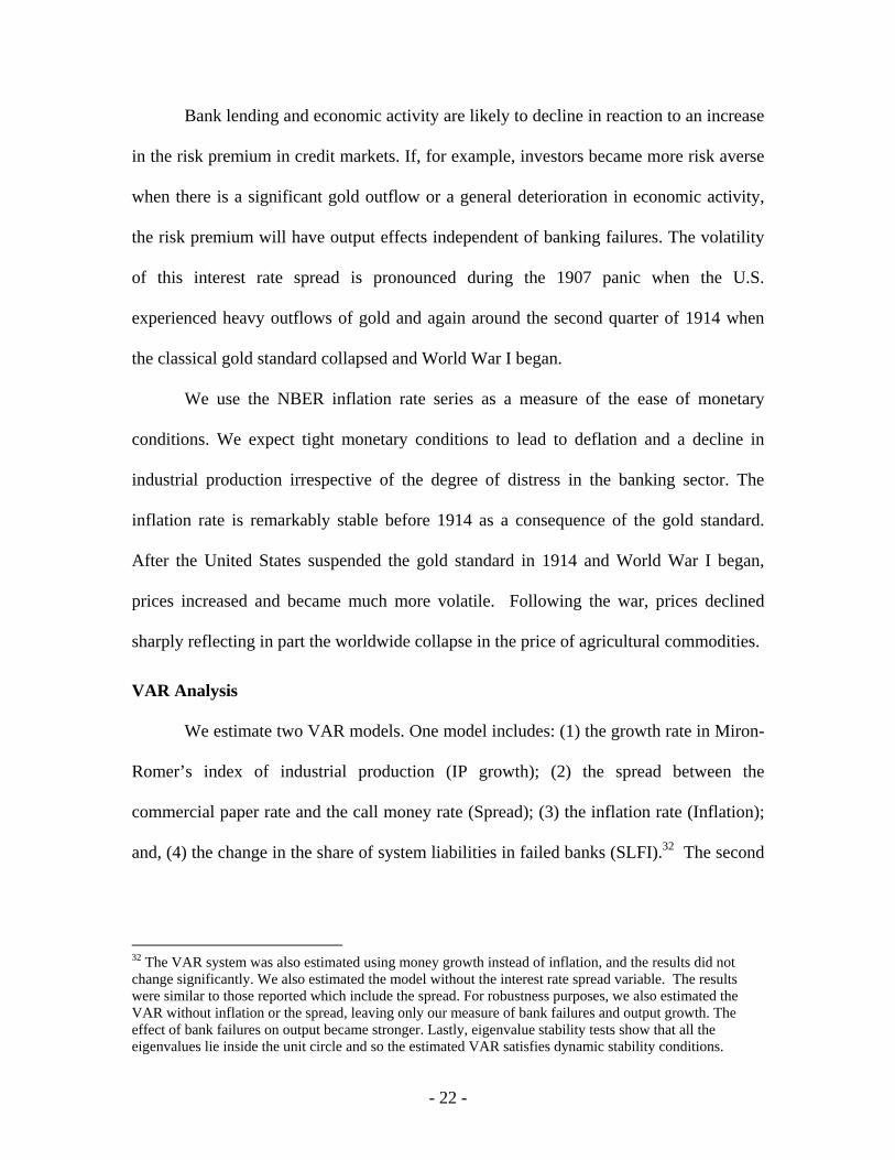
Bank lending and economic activity are likely to decline in reaction to an increase

in the risk premium in credit markets. If, for example, investors became more risk averse

when there is a significant gold outflow or a general deterioration in economic activity,

the risk premium will have output effects independent of banking failures. The volatility

of this interest rate spread is pronounced during the 1907 panic when the U.S.

experienced heavy outflows of gold and again around the second quarter of 1914 when

the classical gold standard collapsed and World War I began.

We use the NBER inflation rate series as a measure of the ease of monetary

conditions. We expect tight monetary conditions to lead to deflation and a decline in

industrial production irrespective of the degree of distress in the banking sector. The

inflation rate is remarkably stable before 1914 as a consequence of the gold standard.

After the United States suspended the gold standard in 1914 and World War I began,

prices increased and became much more volatile. Following the war, prices declined

sharply reflecting in part the worldwide collapse in the price of agricultural commodities.

VAR Analysis

We estimate two VAR models. One model includes: (1) the growth rate in Miron-

Romer’s index of industrial production (IP growth); (2) the spread between the

commercial paper rate and the call money rate (Spread); (3) the inflation rate (Inflation);

and, (4) the change in the share of system liabilities in failed banks (SLFI).32 The second

32 The VAR system was also estimated using money growth instead of inflation, and the results did not change significantly. We also estimated the model without the interest rate spread variable. The results were similar to those reported which include the spread. For robustness purposes, we also estimated the VAR without inflation or the spread, leaving only our measure of bank failures and output growth. The effect of bank failures on output became stronger. Lastly, eigenvalue stability tests show that all the eigenvalues lie inside the unit circle and so the estimated VAR satisfies dynamic stability conditions.

- 23 -

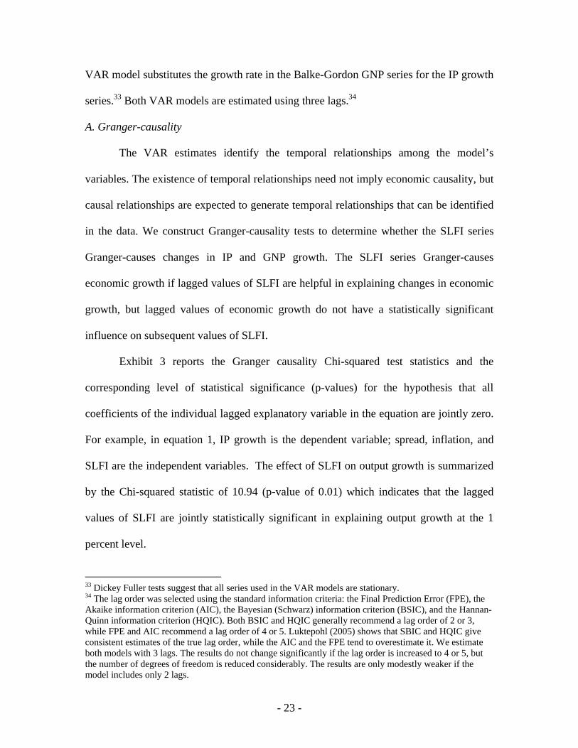
VAR model substitutes the growth rate in the Balke-Gordon GNP series for the IP growth

series.33 Both VAR models are estimated using three lags.34

A. Granger-causality

The VAR estimates identify the temporal relationships among the model’s

variables. The existence of temporal relationships need not imply economic causality, but

causal relationships are expected to generate temporal relationships that can be identified

in the data. We construct Granger-causality tests to determine whether the SLFI series

Granger-causes changes in IP and GNP growth. The SLFI series Granger-causes

economic growth if lagged values of SLFI are helpful in explaining changes in economic

growth, but lagged values of economic growth do not have a statistically significant

influence on subsequent values of SLFI.

Exhibit 3 reports the Granger causality Chi-squared test statistics and the

corresponding level of statistical significance (p-values) for the hypothesis that all

coefficients of the individual lagged explanatory variable in the equation are jointly zero.

For example, in equation 1, IP growth is the dependent variable; spread, inflation, and

SLFI are the independent variables. The effect of SLFI on output growth is summarized

by the Chi-squared statistic of 10.94 (p-value of 0.01) which indicates that the lagged

values of SLFI are jointly statistically significant in explaining output growth at the 1

percent level.

33 Dickey Fuller tests suggest that all series used in the VAR models are stationary. 34 The lag order was selected using the standard information criteria: the Final Prediction Error (FPE), the Akaike information criterion (AIC), the Bayesian (Schwarz) information criterion (BSIC), and the Hannan-Quinn information criterion (HQIC). Both BSIC and HQIC generally recommend a lag order of 2 or 3, while FPE and AIC recommend a lag order of 4 or 5. Luktepohl (2005) shows that SBIC and HQIC give consistent estimates of the true lag order, while the AIC and the FPE tend to overestimate it. We estimate both models with 3 lags. The results do not change significantly if the lag order is increased to 4 or 5, but the number of degrees of freedom is reduced considerably. The results are only modestly weaker if the model includes only 2 lags.

- 24 -

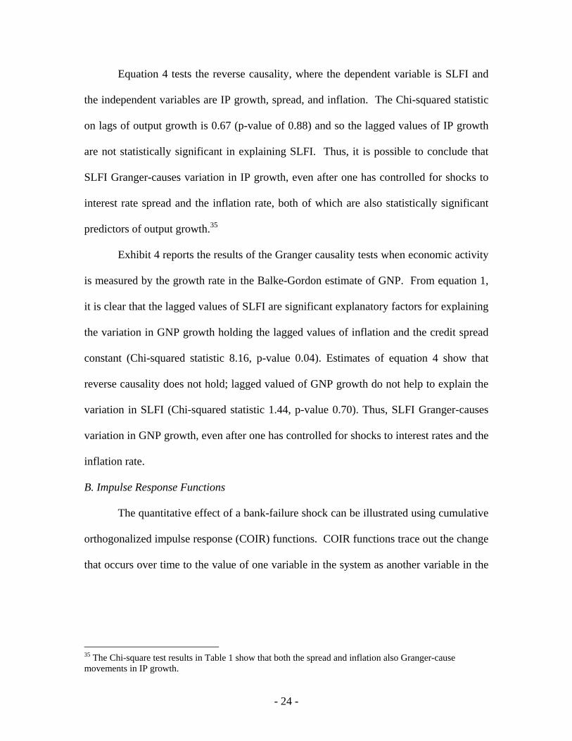
Equation 4 tests the reverse causality, where the dependent variable is SLFI and

the independent variables are IP growth, spread, and inflation. The Chi-squared statistic

on lags of output growth is 0.67 (p-value of 0.88) and so the lagged values of IP growth

are not statistically significant in explaining SLFI. Thus, it is possible to conclude that

SLFI Granger-causes variation in IP growth, even after one has controlled for shocks to

interest rate spread and the inflation rate, both of which are also statistically significant

predictors of output growth.35

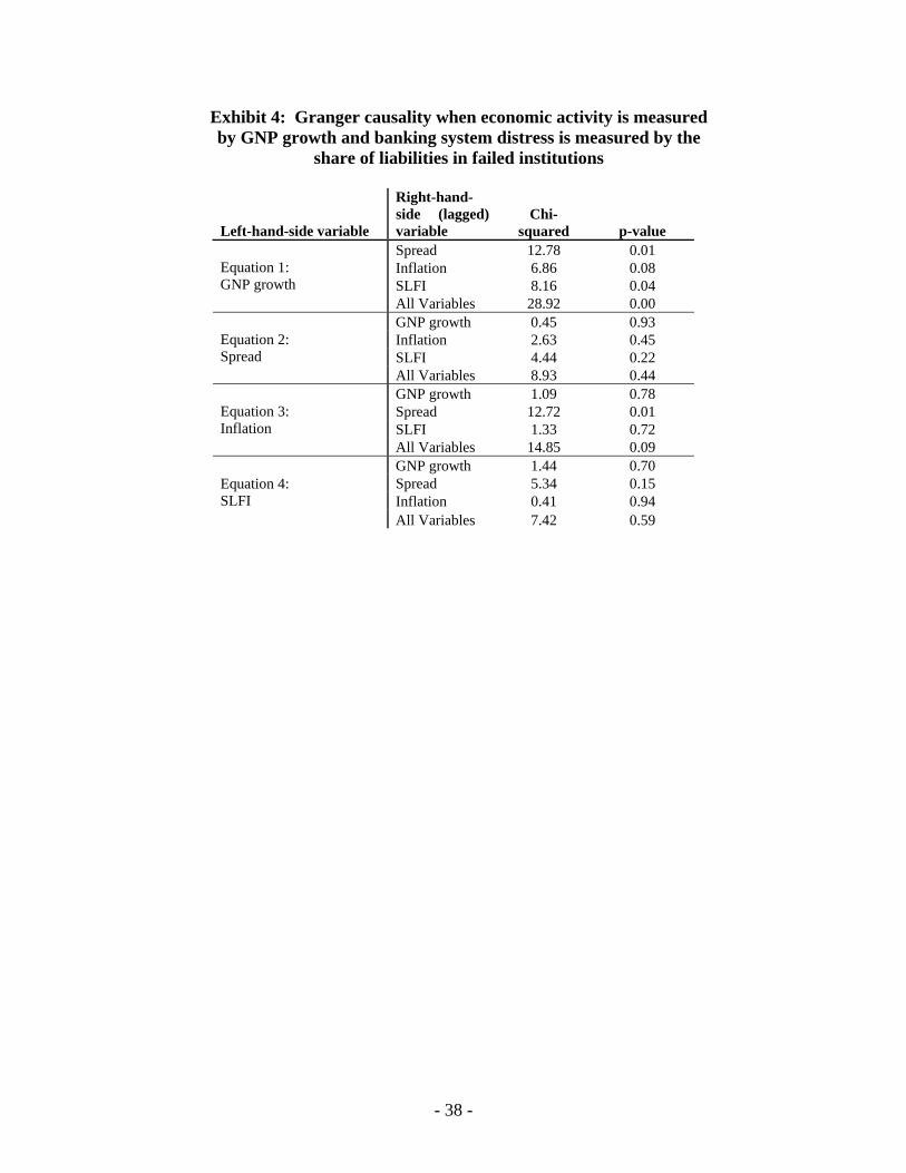
Exhibit 4 reports the results of the Granger causality tests when economic activity

is measured by the growth rate in the Balke-Gordon estimate of GNP. From equation 1,

it is clear that the lagged values of SLFI are significant explanatory factors for explaining

the variation in GNP growth holding the lagged values of inflation and the credit spread

constant (Chi-squared statistic 8.16, p-value 0.04). Estimates of equation 4 show that

reverse causality does not hold; lagged valued of GNP growth do not help to explain the

variation in SLFI (Chi-squared statistic 1.44, p-value 0.70). Thus, SLFI Granger-causes

variation in GNP growth, even after one has controlled for shocks to interest rates and the

inflation rate.

B. Impulse Response Functions

The quantitative effect of a bank-failure shock can be illustrated using cumulative

orthogonalized impulse response (COIR) functions. COIR functions trace out the change

that occurs over time to the value of one variable in the system as another variable in the

35 The Chi-square test results in Table 1 show that both the spread and inflation also Granger-cause movements in IP growth.

- 25 -

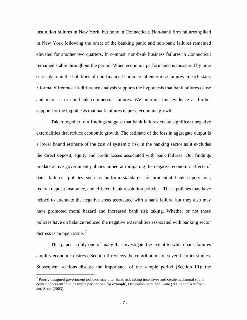
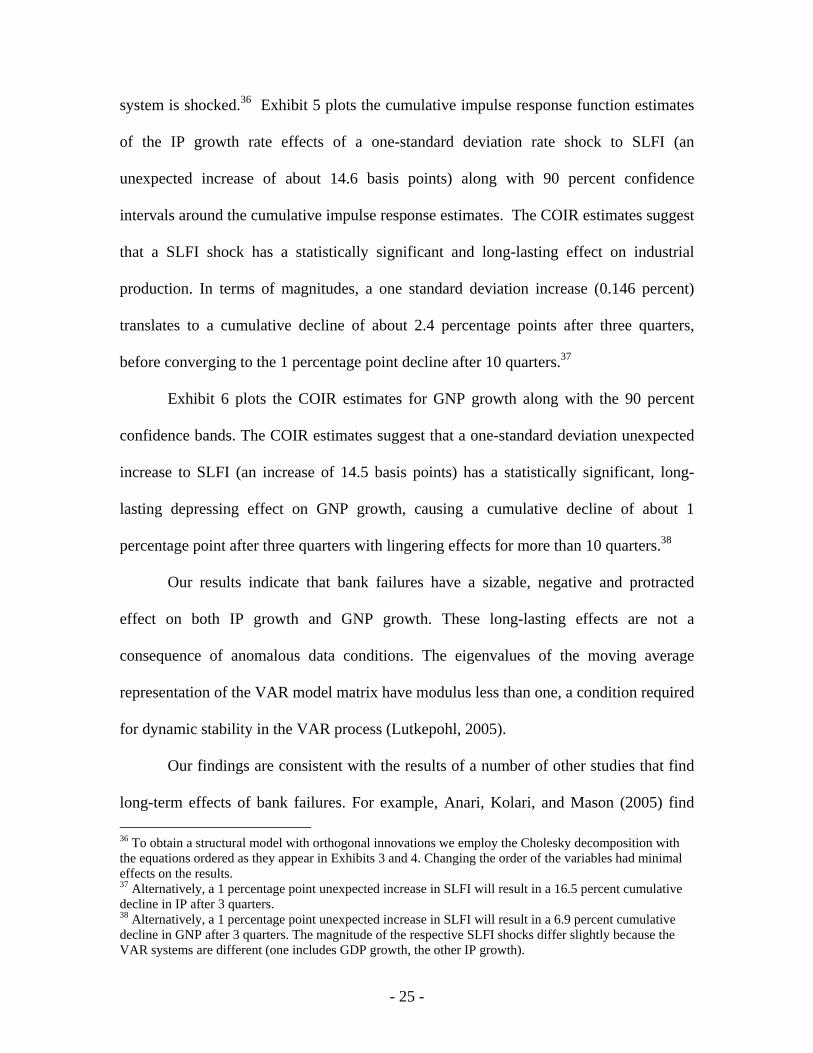
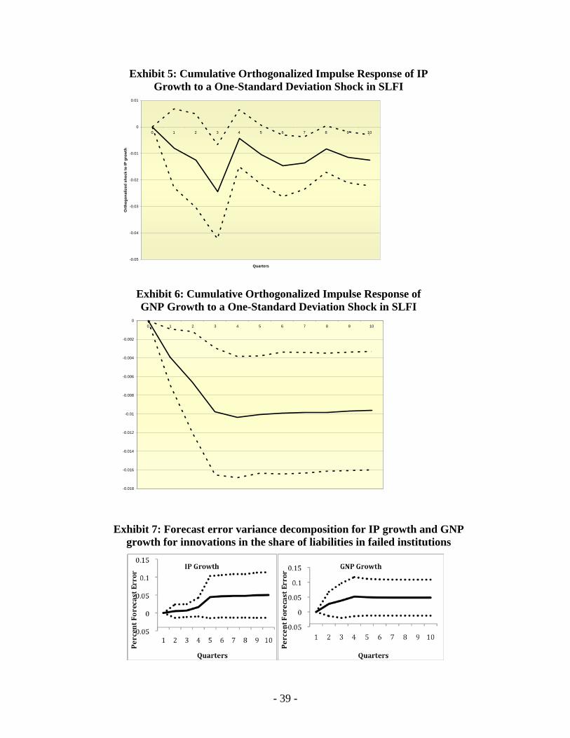
system is shocked.36 Exhibit 5 plots the cumulative impulse response function estimates

of the IP growth rate effects of a one-standard deviation rate shock to SLFI (an

unexpected increase of about 14.6 basis points) along with 90 percent confidence

intervals around the cumulative impulse response estimates. The COIR estimates suggest

that a SLFI shock has a statistically significant and long-lasting effect on industrial

production. In terms of magnitudes, a one standard deviation increase (0.146 percent)

translates to a cumulative decline of about 2.4 percentage points after three quarters,

before converging to the 1 percentage point decline after 10 quarters.37

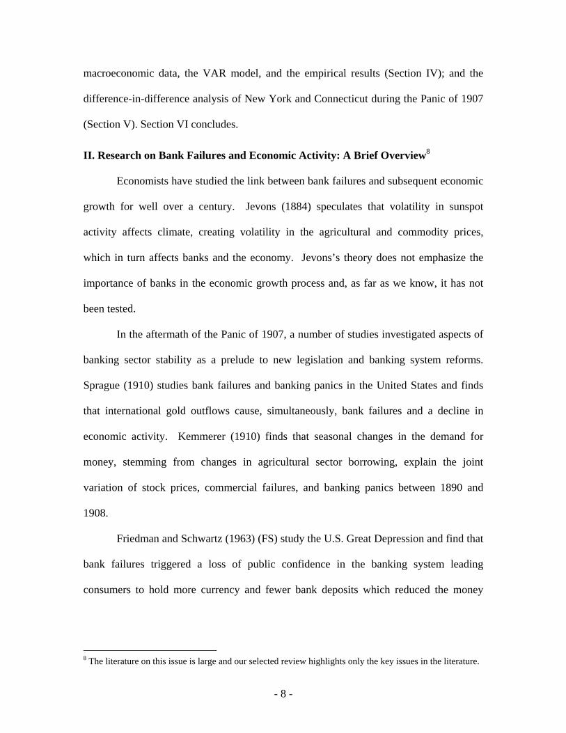
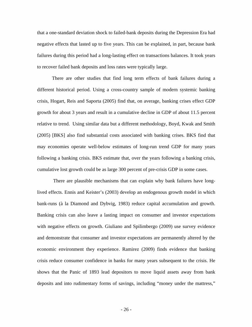
Exhibit 6 plots the COIR estimates for GNP growth along with the 90 percent

confidence bands. The COIR estimates suggest that a one-standard deviation unexpected

increase to SLFI (an increase of 14.5 basis points) has a statistically significant, long-

lasting depressing effect on GNP growth, causing a cumulative decline of about 1

percentage point after three quarters with lingering effects for more than 10 quarters.38

Our results indicate that bank failures have a sizable, negative and protracted

effect on both IP growth and GNP growth. These long-lasting effects are not a

consequence of anomalous data conditions. The eigenvalues of the moving average

representation of the VAR model matrix have modulus less than one, a condition required

for dynamic stability in the VAR process (Lutkepohl, 2005).

Our findings are consistent with the results of a number of other studies that find

long-term effects of bank failures. For example, Anari, Kolari, and Mason (2005) find

36 To obtain a structural model with orthogonal innovations we employ the Cholesky decomposition with the equations ordered as they appear in Exhibits 3 and 4. Changing the order of the variables had minimal effects on the results. 37 Alternatively, a 1 percentage point unexpected increase in SLFI will result in a 16.5 percent cumulative decline in IP after 3 quarters. 38 Alternatively, a 1 percentage point unexpected increase in SLFI will result in a 6.9 percent cumulative decline in GNP after 3 quarters. The magnitude of the respective SLFI shocks differ slightly because the VAR systems are different (one includes GDP growth, the other IP growth).

- 26 -

that a one-standard deviation shock to failed-bank deposits during the Depression Era had

negative effects that lasted up to five years. This can be explained, in part, because bank

failures during this period had a long-lasting effect on transactions balances. It took years

to recover failed bank deposits and loss rates were typically large.

There are other studies that find long term effects of bank failures during a

different historical period. Using a cross-country sample of modern systemic banking

crisis, Hogart, Reis and Saporta (2005) find that, on average, banking crises effect GDP

growth for about 3 years and result in a cumulative decline in GDP of about 11.5 percent

relative to trend. Using similar data but a different methodology, Boyd, Kwak and Smith

(2005) [BKS] also find substantial costs associated with banking crises. BKS find that

may economies operate well-below estimates of long-run trend GDP for many years

following a banking crisis. BKS estimate that, over the years following a banking crisis,

cumulative lost growth could be as large 300 percent of pre-crisis GDP in some cases.

There are plausible mechanisms that can explain why bank failures have long-

lived effects. Ennis and Keister’s (2003) develop an endogenous growth model in which

bank-runs (à la Diamond and Dybvig, 1983) reduce capital accumulation and growth.

Banking crisis can also leave a lasting impact on consumer and investor expectations

with negative effects on growth. Giuliano and Spilimbergo (2009) use survey evidence

and demonstrate that consumer and investor expectations are permanently altered by the

economic environment they experience. Ramirez (2009) finds evidence that banking

crisis reduce consumer confidence in banks for many years subsequent to the crisis. He

shows that the Panic of 1893 lead depositors to move liquid assets away from bank

deposits and into rudimentary forms of savings, including “money under the mattress,”

- 27 -

literally and figuratively. Following the Panic of 1893, people simply stopped trusting

banks which reduced bank’s lending capacity, and growth.

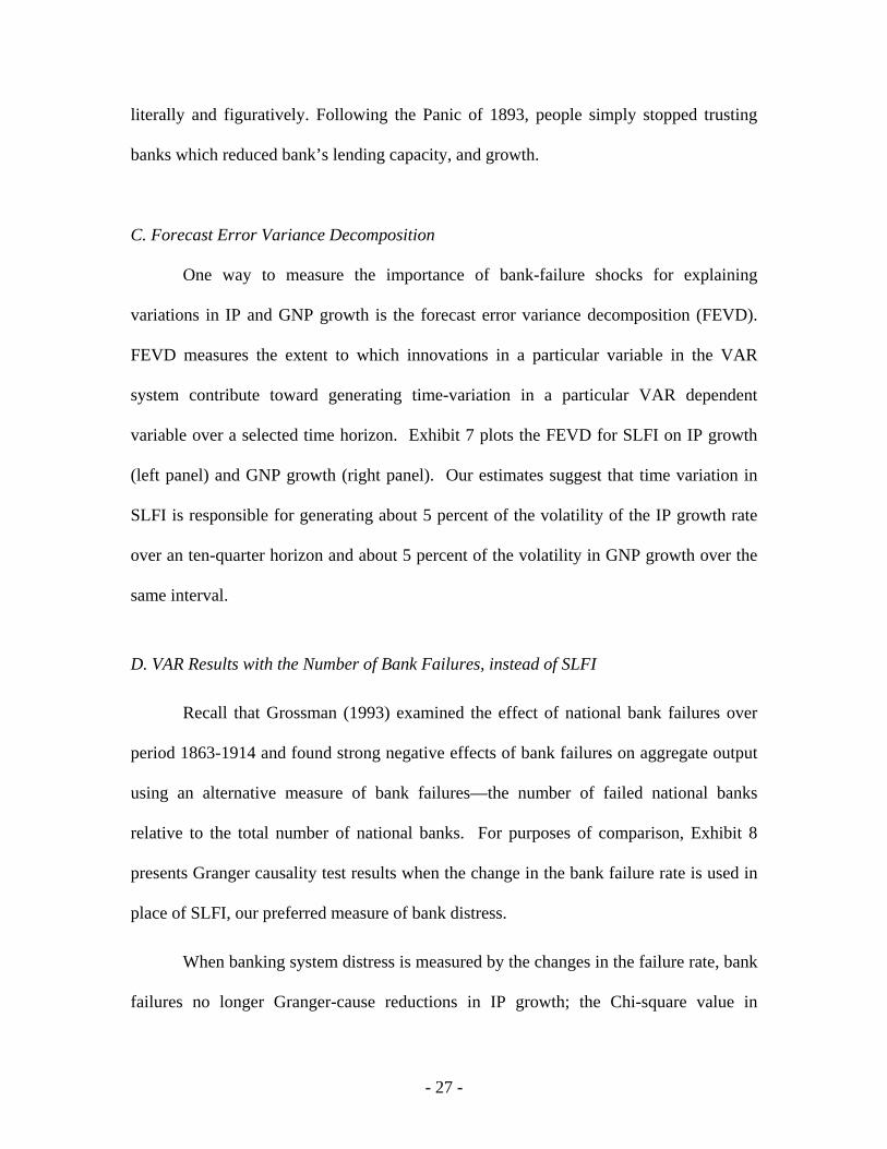
C. Forecast Error Variance Decomposition

One way to measure the importance of bank-failure shocks for explaining

variations in IP and GNP growth is the forecast error variance decomposition (FEVD).

FEVD measures the extent to which innovations in a particular variable in the VAR

system contribute toward generating time-variation in a particular VAR dependent

variable over a selected time horizon. Exhibit 7 plots the FEVD for SLFI on IP growth

(left panel) and GNP growth (right panel). Our estimates suggest that time variation in

SLFI is responsible for generating about 5 percent of the volatility of the IP growth rate

over an ten-quarter horizon and about 5 percent of the volatility in GNP growth over the

same interval.

D. VAR Results with the Number of Bank Failures, instead of SLFI

Recall that Grossman (1993) examined the effect of national bank failures over

period 1863-1914 and found strong negative effects of bank failures on aggregate output

using an alternative measure of bank failures—the number of failed national banks

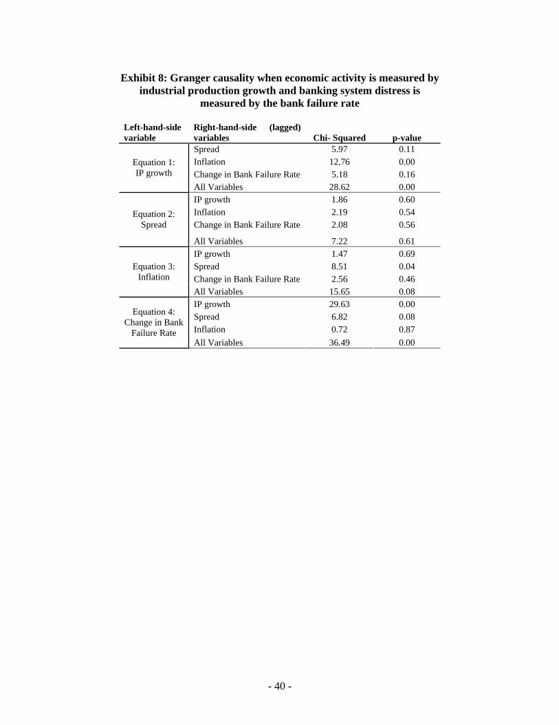
relative to the total number of national banks. For purposes of comparison, Exhibit 8

presents Granger causality test results when the change in the bank failure rate is used in

place of SLFI, our preferred measure of bank distress.

When banking system distress is measured by the changes in the failure rate, bank

failures no longer Granger-cause reductions in IP growth; the Chi-square value in

- 28 -

Exhibit 8, equation 1 (5.18) is not longer statistically significant at conventional levels.39

Moreover, the estimates in equation 4 suggest that lagged values of IP growth are

statistically significant in explaining the bank failure rate. The Chi-square statistic of

29.63 is statistically significant.

These results highlight the importance of the proxy variable used to measure

banking system distress. When banking system distress is measured by the depository

institution failure rate instead of SLFI, banking system distress appears to be caused by

real-side economic disruptions whereas IP growth seems to be unaffected by changes in

the bank failure rate.

V. New York, Connecticut and the Panic of 1907

The Panic of 1907 began in New York in October after an unsuccessful

investment ploy to corner the stock of the United Copper Company. The failed attempt at

cornering the market caused the failure of two brokerage houses. In the days following

the attempt, a number of banks and trusts with direct and indirect links to the cornering

scheme experienced depositor runs. Ultimately, 42 depository institution failures have

been linked to the 1907 Panic (Wicker, 2000, p.87) including 13 depository institution

suspensions in New York in October 1907 (ibid. p.86).40 In contrast to the New York

experience, there were no suspensions of depository institutions in Connecticut.

The financial panic of 1907 occurred against the backdrop of a steep recession

that likely began in the early summer. Industrial production fell by 11 percent between

May 1907 and June 1908; commodity prices fell 21 percent; and unemployment

39 The causality results for GNP growth are similar, so they are omitted in the interest of parsimony. 40 Moen and Tallman (1992) highlight the role of trust companies in aggravating this panic. See also Moen and Tallman (1990).

- 29 -

increased from 2.8 percent to 8 percent.41 While no official GNP estimates are available

for this period, estimates constructed by Romer (1989) suggest that GNP declined by

about 4.2 percent while alternative estimates constructed by Balke-Gordon (1989) put the

decline at 5.5 percent. In another measure of economic activity, the dollar volume of

bankruptcies increased by almost 50 percent November 1907, the month following the

onset of the banking panic.

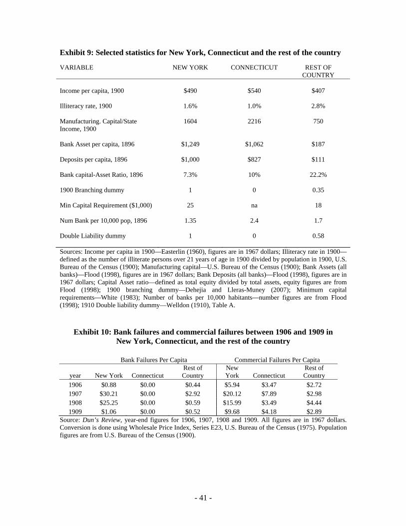
Banking and economic conditions were largely similar in New York and

Connecticut in the years leading up to the panic of 1907. Exhibit 9 presents statistics that

compare economic and banking conditions between New York and Connecticut. At the

turn of century, income per capita estimates suggest that New York was slightly poorer

than Connecticut, but both states enjoyed income levels and literacy rates that were well

above the rest of the country. Both states were heavily involved in the manufacturing

sector: New York’s capital-to-output ratio was more than twice as high as the national

average whereas Connecticut’s was nearly three times as large. In addition, both states

enjoyed high levels of financial depth—bank assets per capita and deposits per capita

were 6 to 7 times larger than the levels for the rest of the country. These figures, along

with the number of banks per 10 thousand inhabitants suggest that banks in New York

and Connecticut were, on average, larger institutions than those in the rest of the country;

New York institutions, moreover, were larger than those in Connecticut.

There are no statistics that can be used to directly assess the ex ante relative risk

of banks in New York compared to those in Connecticut. New York institutions were

larger than those in Connecticut which, holding constant other things, should make them

safer institutions. Although the capital-asset ratio was slightly lower in New York, banks 41 These data are quoted from Bruner and Carr (2007), pp. 141-142 from primary sources.

- 30 -

in that state were allowed to open branches at the time and the literature supports the

hypothesis that branching reduced the probability of failure. Double liability laws have

also been shown to discourage bank risk-taking (Grossman, 2001), and the shareholders

of failing banks in New York were subject to double liability. On balance, there is no

strong reason to believe that bank risk exposures differed significantly across these states.

Overall, the data suggests that conditions in New York and Connecticut are sufficiently

similar prior to 1907 to justify using a difference-in-difference (DID) methodology to

estimate the effect of the Panic of 1907 on economic conditions at the state level.

Exhibit 10 presents summary statistics for the data used to isolate the effect of the

Panic on 1907 on non-bank commercial failures in New York and Connecticut. In 1906,

the liabilities of failed banks in New York amounted to $0.28 per capita. This figure

increased to an average of $10.15 for 1907, and $8.18 for 1908, before returning to

approximately normal (1906) levels in 1909. During this period, Connecticut saw no

failures at all while the remainder of the country experienced bank failures, but at an

intensity level far below the New York experience.

We use the liabilities of non-bank commercial failures per capita (commercial

failures) to measure the effect of bank failure on economic activity.42 Exhibit 10 also

reports these figures for New York, Connecticut, and the rest of the country. Commercial

failures per capita are roughly comparable across the three geographic regions in 1906,

but they increase sharply in New York in 1907 and remain elevated in 1908. While the

commercial failure series more than doubles in Connecticut in 1907, the relative increase

42 Liabilities of bank failures are from Dun’s Review, year-end figures. Liabilities of commercial failures are also from Dun’s Review, year-end figures, and are defined as the sum of the classified failures for manufacturing, trading, and other commercial entities.

- 31 -

is minor compared to New York and, the Connecticut series reverts to its 1906 level by

1908.

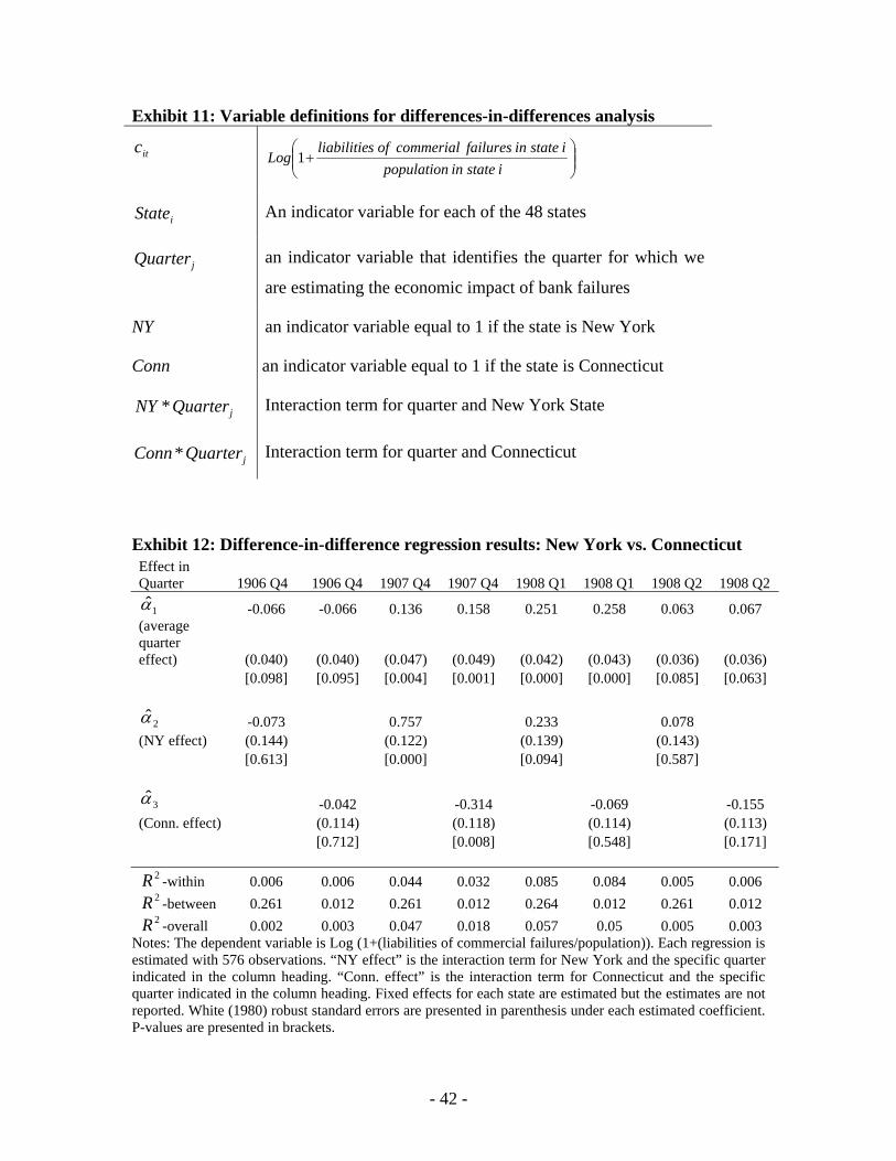
Difference-in-Difference (DID) Test

A DID approach is used to estimate the effect of bank failures on these two states

economies. The approach uses a control group to eliminate the effect of confounding

factors. The variables used in the test are defined in Exhibit 11.

The DID methodology isolates the commercial failure rate in a specific quarter

and estimates the difference in the incidence of commercial failures for New York and

then separately for Connecticut relative to the rest of the country in that specific quarter.

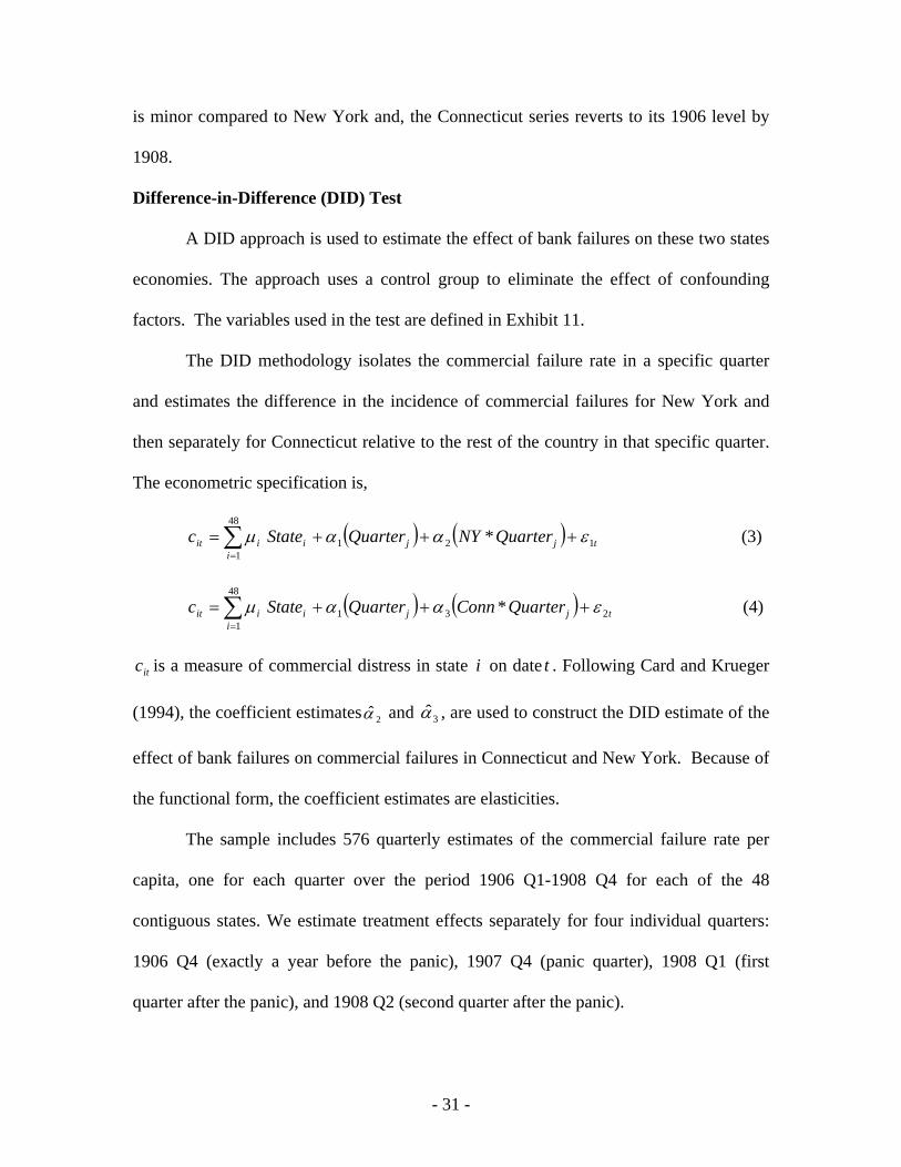
The econometric specification is,

tjjii

iit QuarterNYQuarterStatec 121

48

1

*

(3)

tjjii

iit QuarterConnQuarterStatec 231

48

1

*

(4)

itc is a measure of commercial distress in state i on date t . Following Card and Krueger

(1994), the coefficient estimates 2̂ and 3̂ , are used to construct the DID estimate of the

effect of bank failures on commercial failures in Connecticut and New York. Because of

the functional form, the coefficient estimates are elasticities.

The sample includes 576 quarterly estimates of the commercial failure rate per

capita, one for each quarter over the period 1906 Q1-1908 Q4 for each of the 48

contiguous states. We estimate treatment effects separately for four individual quarters:

1906 Q4 (exactly a year before the panic), 1907 Q4 (panic quarter), 1908 Q1 (first

quarter after the panic), and 1908 Q2 (second quarter after the panic).

- 32 -

Exhibit 12 presents the regression results for the different quarters, starting with

1906 Q4, continuing with 1907 Q4, and 1908 Q1 and 1908 Q2. The first column of

Exhibit 12 reports the treatment effect when the “state” is equal to New York, and the

quarter of interest is 1906 Q4. The estimates suggest that the change in the rate of

commercial failures in New York during the last quarter of 1906 was not statistically

different from the change in the commercial failure rate experienced in all other states.

The coefficient estimate, -0.073, is not statistically significantly different from zero.

The second column of Exhibit 12 estimates the treatment effect for Connecticut in

1906 Q4. For Connecticut, the estimated treatment effect, 042.0 is also not

significantly different from zero indicating that the quarterly change in commercial

failures in Connecticut was close to the change experienced by all other states in 1906

Q4. Thus, exactly one year before the panic took place, business conditions as measured

by the log of business failure liabilities per capita were normal in both New York and

Connecticut relative to conditions in the rest of the country.

The remaining columns in Exhibit 12 show the effects of the banking failures

associated with the Panic of 1907. Beginning in 1907 Q4, the quarter of the banking

panic, the commercial failure experiences of New York and Connecticut diverge

markedly. Column 3 in Exhibit 12 shows that New York experienced a tremendous

increase in commercial distress ( 757.ˆ 2 ), while column 4 shows that Connecticut

experienced a decline in commercial failures ( 314.ˆ3 ). A t-test of the difference of

these two coefficients confirms that commercial failures in New York in 1907 Q4 are

- 33 -

elevated relative to those in Connecticut. 43 Thus, during the panic, it is evident that New

York suffered disproportionately more than the other states in terms of commercial

distress, while Connecticut, if anything, experienced more benign economic conditions.

The regression results reveal that the effects of the banking panic on commercial

distress in New York continued for at least another quarter. The treatment estimate for

1908 Q1 ( 233.ˆ 2 ) is also positive and statistically significant. It is also statistically

different from the 1908 Q1 estimate for Connecticut ( 069.ˆ3 ). The estimates

indicate that economic distress associated with the 1907 banking panic continued in New

York while Connecticut remained unaffected by the crisis. It is not until 1908 Q2 that the

New York treatment coefficient ( 078.ˆ 2 ) indicates that business conditions in New

York returned to normal relative to those prevailing in the rest of the country. These

estimates do not necessarily indicate that business conditions everywhere return to

normal levels during the second quarter of 1908. If commercial distress had spread to the

rest of the nation by 1908 Q2, the situation in New York had converged with conditions

in the rest of the country, but economic conditions could be more challenging than

average in all states.

VI. Concluding Remarks

Using data from 1900 to 1930, a period that predates active government

stabilization policies, we have shown that bank failures have a statistically and

economically important negative effect on economic activity. Our results suggest that an

increase in the share of liabilities in failed depository institutions has a negative and long-

43 The t-test of the difference of these two coefficients is 6.31, which is statistically significant at the less than 1 percent level. The t-test of the difference of these two coefficients at t+1 is 1.68, which is statistically significant at the 5 percent level by a one-tailed test. The coefficients are not statistically different from each other in the other two quarters (t-4 and t+2, where t is the panic quarter).

- 34 -

lasting effect on the growth rate of industrial production and GNP growth. Within three

quarters of the shock, a 1 percent unexpected increase in the liabilities of failed banks is

estimated to cause industrial production to contract by 16.5 percentage points and GNP to

contract by 6.9 percentage points. Estimates suggest that, absent government intervention

to offset the impact of failures, bank failures impose a drag on real economic activity for

at least 10 quarters. To put the magnitude of this shock into perspective, according to

regulatory data, as of 2009 Q4, 14 individual U.S. banks held in excess of 1 percent of

total domestic U.S. deposits.

Our estimates demonstrate that bank failures have important negative externalities

that reduce economic growth and they place a lower bound on the cost of banking sector

systemic risk during this period. Given the magnitude of our estimates, it is perhaps not

surprising that banking policy was an active source of political debate during this era.44

It is tempting to extrapolate our results into modern times and argue that some

form of intervention is necessary to avoid the protracted costs of banking sector systemic

risk. Such inferences, however, are not as straightforward as they may seem. There have

been many important structural changes in the banking sector that may have altered the

cost of systemic risk. These include industry consolidation, the development of bank

holding companies, the removal of prohibitions against interstate branching, and the

growth of international and non-interest sources of bank income and the growth of the so-

called shadow banking sector including securitized lending and money market substitutes

44 Public debate on banking policies began well before the period studied in this paper. State deposit insurance began in 1829 (White, 1983, p. 190) with the founding of the New York Safety Fund. The first national debate on the merits of deposit insurance likely occurred in 1893 when William Jennings Bryan introduced a bill that would establish a national deposit insurance fund (ibid.). Following the Panic of 1907, there was an important national debate focused on banking system reforms designed to enhance bank stability that led ultimately to the creation of the Federal Reserve System in 1913.

- 35 -

for transactions balances. In addition, the banking sector is now subject to many

government policies and regulations—bank deposit insurance, efficient bank resolution

policies, and prudential bank supervision-that likely help mitigate the cost of bank

systemic risk. Given these changes, it is unclear whether a banking crisis in modern

times would result in a protracted contraction in output growth, even in the absence of

active fiscal and monetary policies, typically taken in the aftermath of such events.45

There is another reason for remaining cautious about the necessity of intervention

in the aftermath of banking crises. While government policies may help to mitigate the

effect of bank failures on economic growth, some argue (ourselves included) that these

government policies may also encourage moral hazard and additional bank risk-taking.

The additional risk may create social costs by distorting resource allocation and partly

offset the attenuating effect of government policies the on probability of banking sector

distress. Thus, on balance, it remains unclear whether modern government banking sector

policies should be expected to reduce the costs of systemic risk in the banking sector

relative to those that prevailed in the early twentieth century.

45 Examples of such events in the context of the 2007-09 crisis includes the 2008 federal income tax rebate, the subsidized purchased of Bear Stearns and other open bank assistance programs for institutions under the Federal Reserve, the Treasury, and the FDIC jurisdiction.

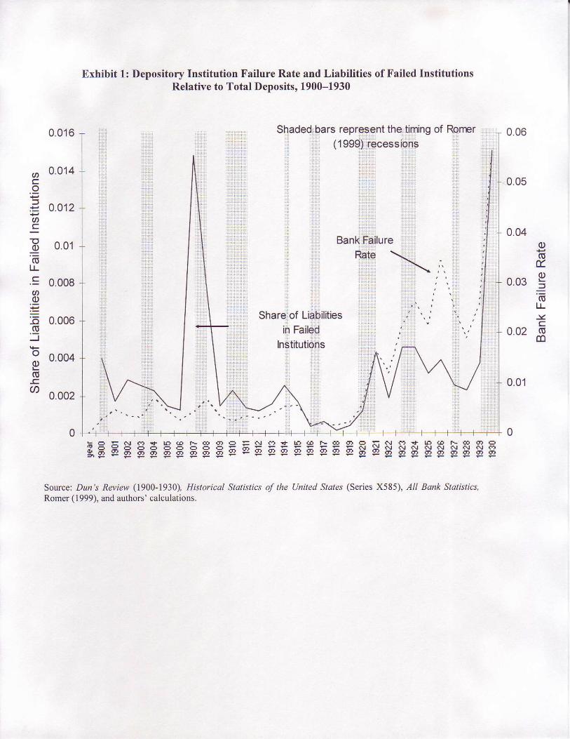
Exhibit 1: Depository Institution Failure Rate and Liabilities of Failed InstitutionsRelative to Total Deposits, 1900-1930

oot-

^^a Ev . v v =

=GLL.!z

0.02 (Em

o

.9f

Eo

=o'6

tL

. ;

,o=b$=

oE(ua

0.016

0.014

0.012

0.01

0.008

0.006

0.004

0.002

0= O = f i l a a + l . 1 @ F S 0 1 O = { \ l ( t ! t l l l t ! F - . t } g t O = f i | C a t t | l l t D l ' L a O 0 1 OqE E E E E E E E E E E P E E E E E F E E f i E E S S S S # S S S

Source: Dr./, b Review (1900-1930), Historical Statistics of the United States (Series X585), All Bank Statistics,Romer (1999), and authors' calculations.

- 37 -

Exhibit 2: Alternative Measures of the Change in Aggregate Economic Activity

-50%

-40%

-30%

-20%

-10%

0%

10%

20%

30%

40%

50%

1900 1905 1910 1915 1920 1925 1930

year

perc

ent c

hang

e

quarterly change in Miron-Romer industrial production index

quarterly change in Balke-Gordon GNP estimates

Source: Gordon (1986, p.781), Miron and Romer (1990, pp. 336-7), and the authors’ calculations.

Exhibit 3: Granger causality when economic activity is measured

by IP growth and banking system distress is measured by the share of liabilities in failed institutions

Left-hand-side variable

Right-hand-side (lagged) variable

Chi- squared p-value

Spread 8.08 0.04 Inflation 16.67 0.00 SLFI 10.94 0.01

Equation 1: IP growth

All Variables 35.50 0.00 IP growth 0.89 0.82 Inflation 2.95 0.40 SLFI 4.17 0.24

Equation 2: Spread

All Variables 9.41 0.40 IP growth 0.72 0.87 Spread 11.12 0.01 SLFI 1.47 0.69

Equation 3: Inflation

All Variables 14.44 0.11 IP growth 0.67 0.88 Spread 5.74 0.13 Inflation 0.07 0.99

Equation 4: SLFI

All Variables 6.61 0.68

- 38 -

Exhibit 4: Granger causality when economic activity is measured by GNP growth and banking system distress is measured by the

share of liabilities in failed institutions

Left-hand-side variable

Right-hand-side (lagged) variable

Chi- squared p-value

Spread 12.78 0.01 Inflation 6.86 0.08 SLFI 8.16 0.04

Equation 1: GNP growth

All Variables 28.92 0.00 GNP growth 0.45 0.93 Inflation 2.63 0.45 SLFI 4.44 0.22

Equation 2: Spread

All Variables 8.93 0.44 GNP growth 1.09 0.78 Spread 12.72 0.01 SLFI 1.33 0.72

Equation 3: Inflation

All Variables 14.85 0.09 GNP growth 1.44 0.70 Spread 5.34 0.15 Inflation 0.41 0.94

Equation 4: SLFI

All Variables 7.42 0.59

- 39 -

Exhibit 5: Cumulative Orthogonalized Impulse Response of IP Growth to a One-Standard Deviation Shock in SLFI

-0.05

-0.04

-0.03

-0.02

-0.01

0

0.01

0 1 2 3 4 5 6 7 8 9 10

Quarters

Ort

ho

go

nal

ized

sh

ock

to

IP g

row

th

Exhibit 6: Cumulative Orthogonalized Impulse Response of GNP Growth to a One-Standard Deviation Shock in SLFI

-0.018

-0.016

-0.014

-0.012

-0.01

-0.008

-0.006

-0.004

-0.002

0

0 1 2 3 4 5 6 7 8 9 10

Exhibit 7: Forecast error variance decomposition for IP growth and GNP

growth for innovations in the share of liabilities in failed institutions

- 40 -

Exhibit 8: Granger causality when economic activity is measured by industrial production growth and banking system distress is

measured by the bank failure rate

Left-hand-side variable

Right-hand-side (lagged) variables Chi- Squared p-value Spread 5.97 0.11 Inflation 12.76 0.00 Change in Bank Failure Rate 5.18 0.16

Equation 1: IP growth

All Variables 28.62 0.00 IP growth 1.86 0.60 Inflation 2.19 0.54 Change in Bank Failure Rate 2.08 0.56

Equation 2: Spread

All Variables 7.22 0.61 IP growth 1.47 0.69 Spread 8.51 0.04 Change in Bank Failure Rate 2.56 0.46

Equation 3: Inflation

All Variables 15.65 0.08 IP growth 29.63 0.00 Spread 6.82 0.08 Inflation 0.72 0.87

Equation 4: Change in Bank

Failure Rate All Variables 36.49 0.00

- 41 -

Exhibit 9: Selected statistics for New York, Connecticut and the rest of the country

VARIABLE NEW YORK CONNECTICUT REST OF COUNTRY

Income per capita, 1900 $490 $540 $407 Illiteracy rate, 1900 1.6% 1.0% 2.8% Manufacturing. Capital/State Income, 1900

1604 2216 750

Bank Asset per capita, 1896 $1,249 $1,062 $187 Deposits per capita, 1896 $1,000 $827 $111 Bank capital-Asset Ratio, 1896 7.3% 10% 22.2% 1900 Branching dummy 1 0 0.35 Min Capital Requirement ($1,000) 25 na 18 Num Bank per 10,000 pop, 1896 1.35 2.4 1.7 Double Liability dummy 1 0 0.58 Sources: Income per capita in 1900—Easterlin (1960), figures are in 1967 dollars; Illiteracy rate in 1900—defined as the number of illiterate persons over 21 years of age in 1900 divided by population in 1900, U.S. Bureau of the Census (1900); Manufacturing capital—U.S. Bureau of the Census (1900); Bank Assets (all banks)—Flood (1998), figures are in 1967 dollars; Bank Deposits (all banks)—Flood (1998), figures are in 1967 dollars; Capital Asset ratio—defined as total equity divided by total assets, equity figures are from Flood (1998); 1900 branching dummy—Dehejia and Lleras-Muney (2007); Minimum capital requirements—White (1983); Number of banks per 10,000 habitants—number figures are from Flood (1998); 1910 Double liability dummy—Welldon (1910), Table A.

Exhibit 10: Bank failures and commercial failures between 1906 and 1909 in New York, Connecticut, and the rest of the country

Bank Failures Per Capita Commercial Failures Per Capita

year New York Connecticut Rest of Country

New York Connecticut

Rest of Country

1906 $0.88 $0.00 $0.44 $5.94 $3.47 $2.72 1907 $30.21 $0.00 $2.92 $20.12 $7.89 $2.98 1908 $25.25 $0.00 $0.59 $15.99 $3.49 $4.44 1909 $1.06 $0.00 $0.52 $9.68 $4.18 $2.89

Source: Dun’s Review, year-end figures for 1906, 1907, 1908 and 1909. All figures are in 1967 dollars. Conversion is done using Wholesale Price Index, Series E23, U.S. Bureau of the Census (1975). Population figures are from U.S. Bureau of the Census (1900).

- 42 -

Exhibit 11: Variable definitions for differences-in-differences analysis

itc

istateinpopulation

istateinfailurescommerialofsliabilitieLog 1

iState An indicator variable for each of the 48 states

jQuarter an indicator variable that identifies the quarter for which we

are estimating the economic impact of bank failures

NY an indicator variable equal to 1 if the state is New York

Conn a an indicator variable equal to 1 if the state is Connecticut

jQuarterNY * Interaction term for quarter and New York State

jQuarterConn * Interaction term for quarter and Connecticut

Exhibit 12: Difference-in-difference regression results: New York vs. Connecticut Effect in

Quarter 1906 Q4 1906 Q4 1907 Q4 1907 Q4 1908 Q1 1908 Q1 1908 Q2 1908 Q2

1̂ -0.066 -0.066 0.136 0.158 0.251 0.258 0.063 0.067 (average quarter effect) (0.040) (0.040) (0.047) (0.049) (0.042) (0.043) (0.036) (0.036) [0.098] [0.095] [0.004] [0.001] [0.000] [0.000] [0.085] [0.063]

2̂ -0.073 0.757 0.233 0.078 (NY effect) (0.144) (0.122) (0.139) (0.143) [0.613] [0.000] [0.094] [0.587]

3̂ -0.042 -0.314 -0.069 -0.155 (Conn. effect) (0.114) (0.118) (0.114) (0.113) [0.712] [0.008] [0.548] [0.171]

2R -within 0.006 0.006 0.044 0.032 0.085 0.084 0.005 0.006 2R -between 0.261 0.012 0.261 0.012 0.264 0.012 0.261 0.012 2R -overall 0.002 0.003 0.047 0.018 0.057 0.05 0.005 0.003

Notes: The dependent variable is Log (1+(liabilities of commercial failures/population)). Each regression is estimated with 576 observations. “NY effect” is the interaction term for New York and the specific quarter indicated in the column heading. “Conn. effect” is the interaction term for Connecticut and the specific quarter indicated in the column heading. Fixed effects for each state are estimated but the estimates are not reported. White (1980) robust standard errors are presented in parenthesis under each estimated coefficient. P-values are presented in brackets.

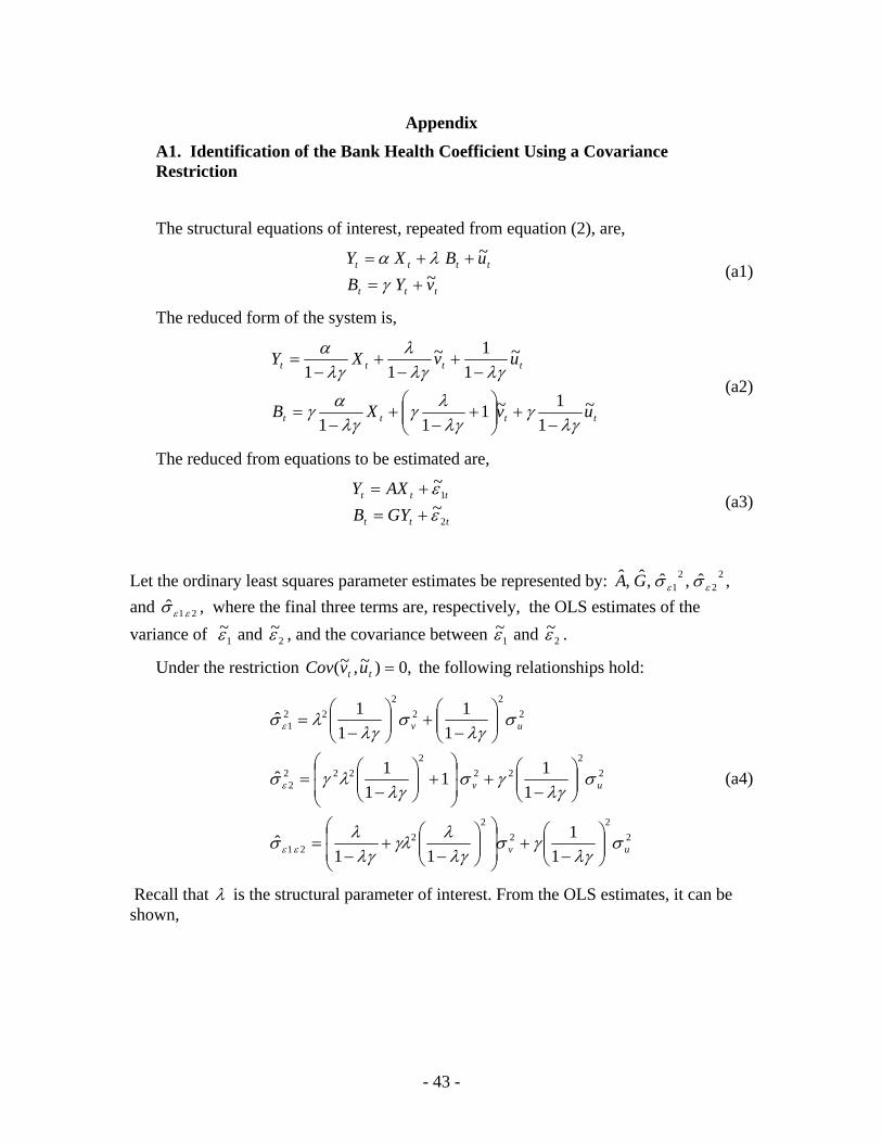
- 43 -

Appendix

A1. Identification of the Bank Health Coefficient Using a Covariance Restriction

The structural equations of interest, repeated from equation (2), are,

ttt

tttt

vYB

uBXY~

~

(a1)

The reduced form of the system is,

tttt

tttt

uvXB

uvXY

~1

1~111

~1

1~11

(a2)

The reduced from equations to be estimated are,

ttt

ttt

GYB

AXY

2

1

~

~

(a3)

Let the ordinary least squares parameter estimates be represented by: ,ˆ,ˆ,ˆ,ˆ 22

21 GA

and 21ˆ , where the final three terms are, respectively, the OLS estimates of the

variance of 1~ and 2

~ , and the covariance between 1~ and 2

~ .

Under the restriction ,0)~,~( tt uvCov the following relationships hold:

2

2

2

2

221

2

2

22

2

2222

2

2

2

2

221

1

1

11ˆ

1

11

1

1ˆ

1

1

1

1ˆ

uv

uv

uv

(a4)

Recall that is the structural parameter of interest. From the OLS estimates, it can be shown,

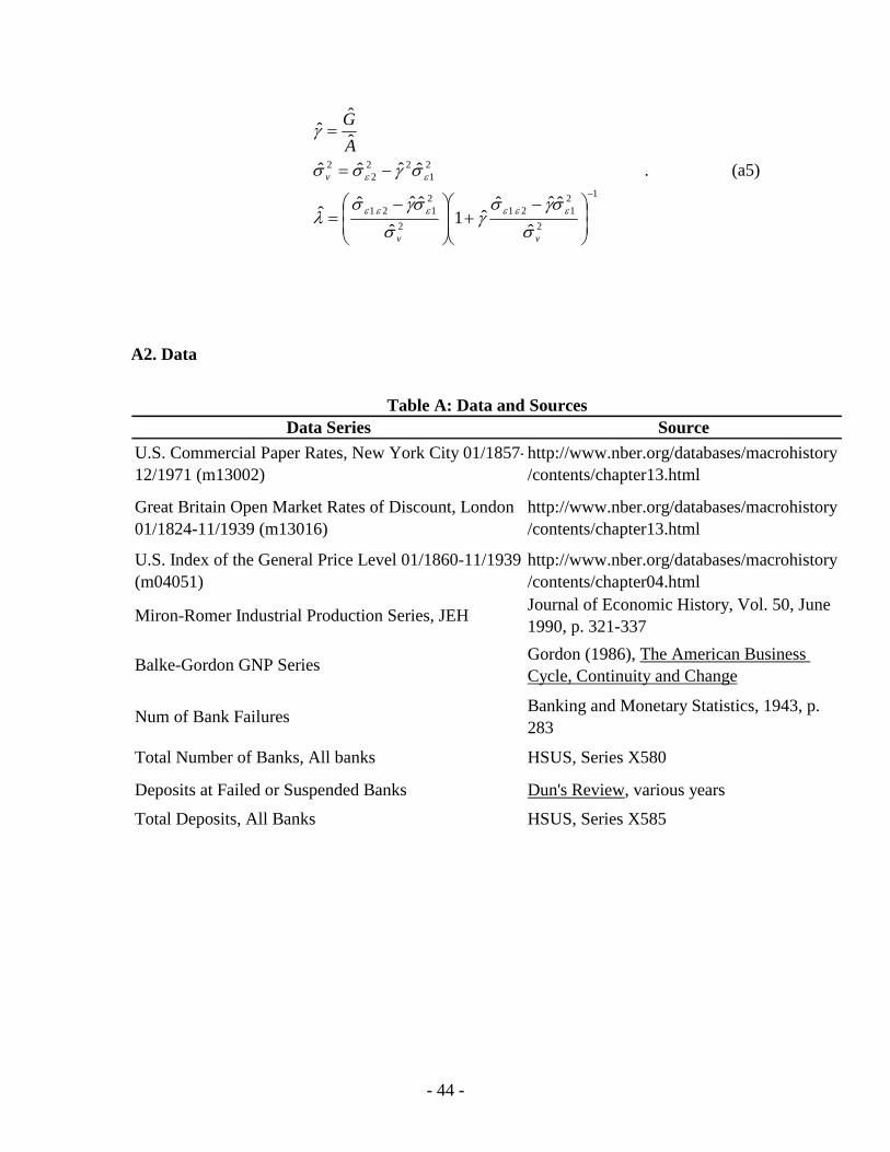
- 44 -

1

2

2121

2

2121

21

222

2

ˆ

ˆˆˆˆ1

ˆ

ˆˆˆˆ

ˆˆˆˆ

ˆ

ˆˆ

vv

v

A

G

. (a5)

A2. Data

Data Series Source

U.S. Commercial Paper Rates, New York City 01/1857-12/1971 (m13002)

http://www.nber.org/databases/macrohistory/contents/chapter13.html

Great Britain Open Market Rates of Discount, London 01/1824-11/1939 (m13016)

http://www.nber.org/databases/macrohistory/contents/chapter13.html

U.S. Index of the General Price Level 01/1860-11/1939 (m04051)

http://www.nber.org/databases/macrohistory/contents/chapter04.html

Miron-Romer Industrial Production Series, JEHJournal of Economic History, Vol. 50, June 1990, p. 321-337

Balke-Gordon GNP SeriesGordon (1986), The American Business Cycle, Continuity and Change

Num of Bank FailuresBanking and Monetary Statistics, 1943, p. 283

Total Number of Banks, All banks HSUS, Series X580

Deposits at Failed or Suspended Banks Dun's Review, various years

Total Deposits, All Banks HSUS, Series X585

Table A: Data and Sources

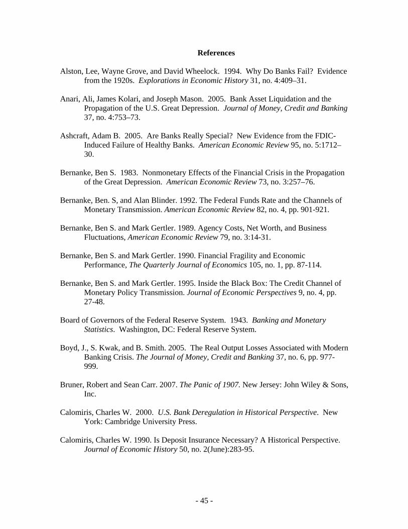
- 45 -

References

Alston, Lee, Wayne Grove, and David Wheelock. 1994. Why Do Banks Fail? Evidence from the 1920s. Explorations in Economic History 31, no. 4:409–31.

Anari, Ali, James Kolari, and Joseph Mason. 2005. Bank Asset Liquidation and the

Propagation of the U.S. Great Depression. Journal of Money, Credit and Banking 37, no. 4:753–73.

Ashcraft, Adam B. 2005. Are Banks Really Special? New Evidence from the FDIC-

Induced Failure of Healthy Banks. American Economic Review 95, no. 5:1712–30.

Bernanke, Ben S. 1983. Nonmonetary Effects of the Financial Crisis in the Propagation

of the Great Depression. American Economic Review 73, no. 3:257–76. Bernanke, Ben. S, and Alan Blinder. 1992. The Federal Funds Rate and the Channels of

Monetary Transmission. American Economic Review 82, no. 4, pp. 901-921. Bernanke, Ben S. and Mark Gertler. 1989. Agency Costs, Net Worth, and Business

Fluctuations, American Economic Review 79, no. 3:14-31. Bernanke, Ben S. and Mark Gertler. 1990. Financial Fragility and Economic

Performance, The Quarterly Journal of Economics 105, no. 1, pp. 87-114. Bernanke, Ben S. and Mark Gertler. 1995. Inside the Black Box: The Credit Channel of

Monetary Policy Transmission. Journal of Economic Perspectives 9, no. 4, pp. 27-48.

Board of Governors of the Federal Reserve System. 1943. Banking and Monetary

Statistics. Washington, DC: Federal Reserve System. Boyd, J., S. Kwak, and B. Smith. 2005. The Real Output Losses Associated with Modern

Banking Crisis. The Journal of Money, Credit and Banking 37, no. 6, pp. 977-999.

Bruner, Robert and Sean Carr. 2007. The Panic of 1907. New Jersey: John Wiley & Sons,

Inc. Calomiris, Charles W. 2000. U.S. Bank Deregulation in Historical Perspective. New

York: Cambridge University Press. Calomiris, Charles W. 1990. Is Deposit Insurance Necessary? A Historical Perspective.

Journal of Economic History 50, no. 2(June):283-95.

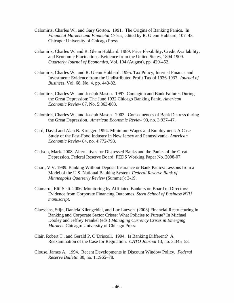
- 46 -

Calomiris, Charles W., and Gary Gorton. 1991. The Origins of Banking Panics. In Financial Markets and Financial Crises, edited by R. Glenn Hubbard, 107–43. Chicago: University of Chicago Press.

Calomiris, Charles W. and R. Glenn Hubbard. 1989. Price Flexibility, Credit Availability,

and Economic Fluctuations: Evidence from the United States, 1894-1909. Quarterly Journal of Economics, Vol. 104 (August), pp. 429-452.

Calomiris, Charles W., and R. Glenn Hubbard. 1995. Tax Policy, Internal Finance and

Investment: Evidence from the Undistributed Profit Tax of 1936-1937. Journal of Business, Vol. 68, No. 4, pp. 443-82.

Calomiris, Charles W., and Joseph Mason. 1997. Contagion and Bank Failures During

the Great Depression: The June 1932 Chicago Banking Panic. American Economic Review 87, No. 5:863-883.

Calomiris, Charles W., and Joseph Mason. 2003. Consequences of Bank Distress during

the Great Depression. American Economic Review 93, no. 3:937–47. Card, David and Alan B. Krueger. 1994. Minimum Wages and Employment: A Case

Study of the Fast-Food Industry in New Jersey and Pennsylvania. American Economic Review 84, no. 4:772-793.

Carlson, Mark. 2008. Alternatives for Distressed Banks and the Panics of the Great

Depression. Federal Reserve Board: FEDS Working Paper No. 2008-07. Chari, V.V. 1989. Banking Without Deposit Insurance or Bank Panics: Lessons from a

Model of the U.S. National Banking System. Federal Reserve Bank of Minneapolis Quarterly Review (Summer): 3-19.

Ciamarra, Elif Sisli. 2006. Monitoring by Affiliated Bankers on Board of Directors:

Evidence from Corporate Financing Outcomes. Stern School of Business NYU manuscript.

Claessens, Stijn, Daniela Kliengebiel, and Luc Laeven. (2003) Financial Restructuring in

Banking and Corporate Sector Crises: What Policies to Pursue? In Michael Dooley and Jeffrey Frankel (eds.) Managing Currency Crises in Emerging Markets. Chicago: University of Chicago Press.

Clair, Robert T., and Gerald P. O’Driscoll. 1994. Is Banking Different? A

Reexamination of the Case for Regulation. CATO Journal 13, no. 3:345–53. Clouse, James A. 1994. Recent Developments in Discount Window Policy. Federal

Reserve Bulletin 80, no. 11:965–78.

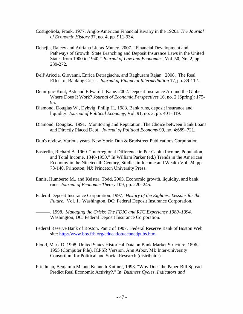
- 47 -

Costigoliola, Frank. 1977. Anglo-American Financial Rivalry in the 1920s. The Journal of Economic History 37, no. 4, pp. 911-934.

Dehejia, Rajeev and Adriana Lleras-Muney. 2007. “Financial Development and

Pathways of Growth: State Branching and Deposit Insurance Laws in the United States from 1900 to 1940,” Journal of Law and Economics, Vol. 50, No. 2, pp. 239-272.

Dell’Ariccia, Giovanni, Enrica Detragiache, and Raghuram Rajan. 2008. The Real

Effect of Banking Crises. Journal of Financial Intermediation 17, pp. 89-112. Demirguc-Kunt, Asli and Edward J. Kane. 2002. Deposit Insurance Around the Globe:

Where Does It Work? Journal of Economic Perspectives 16, no. 2 (Spring): 175-95.

Diamond, Douglas W., Dybvig, Philip H., 1983. Bank runs, deposit insurance and liquidity. Journal of Political Economy, Vol. 91, no. 3, pp. 401–419.

Diamond, Douglas. 1991. Monitoring and Reputation: The Choice between Bank Loans

and Directly Placed Debt. Journal of Political Economy 99, no. 4:689–721. Dun's review. Various years. New York: Dun & Bradstreet Publications Corporation. Easterlin, Richard A. 1960. “Interregional Difference in Per Capita Income, Population,

and Total Income, 1840-1950.” In William Parker (ed.) Trends in the American Economy in the Nineteenth Century, Studies in Income and Wealth Vol. 24, pp. 73-140. Princeton, NJ: Princeton University Press.

Ennis, Humberto M., and Keister, Todd, 2003. Economic growth, liquidity, and bank

runs. Journal of Economic Theory 109, pp. 220–245. Federal Deposit Insurance Corporation. 1997. History of the Eighties: Lessons for the

Future. Vol. 1. Washington, DC: Federal Deposit Insurance Corporation. ———. 1998. Managing the Crisis: The FDIC and RTC Experience 1980–1994.

Washington, DC: Federal Deposit Insurance Corporation. Federal Reserve Bank of Boston. Panic of 1907. Federal Reserve Bank of Boston Web

site: http://www.bos.frb.org/education/econedpubs.htm. Flood, Mark D. 1998. United States Historical Data on Bank Market Structure, 1896-

1955 (Computer File). ICPSR Version. Ann Arbor, MI: Inter-university Consortium for Political and Social Research (distributor).

Friedman, Benjamin M. and Kenneth Kuttner, 1993. "Why Does the Paper-Bill Spread

Predict Real Economic Activity?," In: Business Cycles, Indicators and

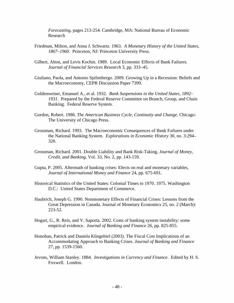
- 48 -

Forecasting, pages 213-254. Cambridge, MA: National Bureau of Economic Research

Friedman, Milton, and Anna J. Schwartz. 1963. A Monetary History of the United States,

1867–1960. Princeton, NJ: Princeton University Press. Gilbert, Alton, and Levis Kochin. 1989. Local Economic Effects of Bank Failures.

Journal of Financial Services Research 3, pp. 333–45. Giuliano, Paola, and Antonio Spilimbergo. 2009. Growing Up in a Recession: Beliefs and

the Macroeconomy, CEPR Discussion Paper 7399. Goldenweiser, Emanuel A., et al. 1932. Bank Suspensions in the United States, 1892–

1931. Prepared by the Federal Reserve Committee on Branch, Group, and Chain Banking. Federal Reserve System.

Gordon, Robert. 1986. The American Business Cycle, Continuity and Change. Chicago:

The University of Chicago Press. Grossman, Richard. 1993. The Macroeconomic Consequences of Bank Failures under

the National Banking System. Explorations in Economic History 30, no. 3:294–320.

Grossman, Richard. 2001. Double Liability and Bank Risk-Taking, Journal of Money,

Credit, and Banking, Vol. 33, No. 2, pp. 143-159. Gupta, P. 2005. Aftermath of banking crises: Efects on real and monetary variables,

Journal of International Money and Finance 24, pp. 675-691. Historical Statistics of the United States: Colonial Times to 1970. 1975. Washington

D.C.: United States Department of Commerce. Haubrich, Joseph G. 1990. Nonmonetary Effects of Financial Crises: Lessons from the

Great Depression in Canada. Journal of Monetary Economics 25, no. 2 (March): 223-52.

Hogart, G., R. Reis, and V. Saporta. 2002. Costs of banking system instability: some

empirical evidence. Journal of Banking and Finance 26, pp. 825-855. Honohan, Patrick and Daniela Klingebiel (2003). The Fiscal Cost Implications of an

Accommodating Approach to Banking Crises. Journal of Banking and Finance 27, pp. 1539-1560.

Jevons, William Stanley. 1884. Investigations in Currency and Finance. Edited by H. S.

Foxwell. London.

- 49 -

Kane, Edward. 1989. The High Cost of Incompletely Funding the FSLIC Shortage of Explicit Capital. The Journal of Economic Perspectives 3, no. 4, pp. 31-47.

Kaufmann, George G., and Kenneth E. Scott. 2003. What Is Systemic Risk, and Do

Bank Regulators Retard or Contribute to It? Independent Review: A Journal of Political Economy 7, no. 3,pp. 371–91.

Kemmerer, Edwin W. 1910. Seasonal Variations in the Relative Demand for Money and

Capital in the United States. National Monetary Commission, Senate Document 588, 61st Cong., 2nd sess.

Kormendi, Roger C., Victor L. Bernard, S. Craig Pirrong, and Edward A. Snyder. 1989.

Crisis Resolution in the Thrift Industry: Beyond the December Deals. Report of the Mid America Institute Task Force on the Thrift Crisis. University of Michigan.

Kroszner, Randall S. 2006. The Effect of Removing Geographic Restrictions on Banking

in the United States: Lessons for Europe. Remarks presented at the Conference on the Future of Financial Regulation. London School of Economics, London.

Kroszner, R., L, Laeven, and D. Klingebiel. 2007. Banking crisis, financial dependence

and growth. Journal of Financial Economics 84, no. 1, pp.187-228. Lütkepohl, Helmut. 2005. New Introduction to Multiple Time Series Analysis. Berlin:

Springer-Verlag. Meltzer, Allan. 2003. A History of the Federal Reserve: Volume I, 1913-1951. Chicago:

The University of Chicago Press. Miron, Jeffrey A. 1986. Financial Panics, the Seasonality of the Nominal Interest Rate,

and the Founding of the Fed. American Economic Review 76 (March), pp. 125-40. Miron, Jeffrey, A. and Christina D. Romer. 1990. A New Monthly Index of Industrial

Production, 1884–1940. Journal of Economic History 50 (June), pp. 321–37. Moen, Jon R. and Ellis W. Tallman. 1990. Lessons from the Panic of 1907. Federal

Reserve Bank of Atlanta Economic Review, May/June, pp. 2-13. Moen, Jon R. and Ellis W. Tallman. 1992. The Bank Panic of 1907: The Role of Trust

Companies. Journal of Economic History 52, no. 3 (Sept), pp. 611-630. Mussa, Michael. 1994. U.S. Monetary Policy in the 1980s. In American Economic

Policy in the 1980s, edited by Martin S. Feldstein, chap. 2. Chicago, IL: University of Chicago Press.

- 50 -

Peek, Joe, and Eric Rosengren 1995. The Capital Crunch: Neither a Borrower or a Lender Be. Journal of Money, Credit and Banking 27, no.3, pp. 625-38.

Rajan, Raghuram. 1992. Insiders and Outsiders: The Choice between Informed and

Arm’s Length Debt. Journal of Finance 47, no. 4, pp.1367–1400. Ramirez, Carlos D. 1999. Did Glass-Steagall Increase the Cost of External Finance for

Corporate Investment? Evidence from Bank and Insurance Company Affiliations. Journal of Economic History 59, no. 2, pp. 372–96.

Ramirez, Carlos D. 2009. Bank Fragility, “Money Under the Mattress,” and Long-Run

Growth: US Evidence from the “Perfect” Panic of 1893. Journal of Banking and Finance 33, no. 12, pp. 2185 -2198.

Redlich, Fritz. 1951. The Moulding of American Banking, Men and Ideas, Part II, 1840–

1910. New York: Hafner Publishing Company. Romer, Christina D. 1989. The Prewar Business Cycle Reconsidered: New Estimates of

Gross National Product, 1869-1908. Journal of Political Economy 97, no. 1, pp. 1-37.

Romer, Christina D. 1999. Changes in Business Cycles: Evidence and Explanations.

Journal of Economic Perspectives 13, no. 2, pp. 23–44. ———. 2002. Business Cycles. In The Concise Encyclopedia of Economics, edited by

David R. Henderson. Indianapolis, IN: Liberty Fund, Inc. Online, available from http://www.econlib.org/Library/Enc/BusinessCycles.html.

Romer, Thomas and Barry Weingast. 1991. Political Foundations of the Thrift Debacle,

in Politics and Economics in the Eighties. Alberto Alesina and Geoffrey Carliner editors. Chicago: University of Chicago Press, pp. 175-214.

Schwartz, Steven. 2008. Systemic Risk. Georgetown Law Journal 97, no. 1. Sprague, Oliver M. W. 1910. History of Crises under the National Banking System.

Washington, DC: National Monetary Commission. Stiglitz, Joseph, and Andrew Weiss. 1981. Credit Rationing in Markets with Imperfect

Information. American Economic Review 71, no. 3, pp. 393–410. Stock, James H. and Mark W. Watson. 1989. New Indexes of Coincident and Leading

Economic Indicators. In Oliver Blanchard and Stanley Fischer (eds.) NBER Macroeconomics Annual 1989. Cambridge, MA: MIT Press.

U.S. Bureau of the Census. 1900. Twelfth Census of the United States (1900), Volumes 1

through 10. Washington, DC: Government Printing Office

- 51 -

Webb, David. 1991. Long-Term Financial Contracts Can Mitigate the Adverse Selection

Problem in Project Financing. International Economic Review 32, no. 2, pp. 305–320.

Welldon, Samuel A. 1910. Digest of State Banking Statutes. National Monetary

Commission, 61st Congress, 2nd session, Senate Document No. 353. Washington, DC.

Wheelock, David C. 1992. Regulation and Bank Failures: New Evidence from the

Agricultural Collapse of the 1920s. Journal of Economic History 52, pp. 806–825.

Wheelock, David C., and Paul W. Wilson. 1994. Can Deposit Insurance Increase the

Risk of Bank Failure? Some Historical Evidence. Federal Reserve Bank of St. Louis Economic Review (May/June), pp. 57–71.

White, Eugene N. 1983. Regulation and Reform of the American Banking System, 1900-

1929. Princeton University Press, Princeton, NJ. White, Eugene N. 1984. “A Reinterpretation of the Banking Crisis of 1930.” Journal of

Economic History 44, pp. 119-138. White, Halbert. 1980. “A Heteroskedasticity-consistent Covariance Matrix Estimator and

a Direct Test for Heteroskedasticity,” Econometrica 48, pp. 817-838. Wicker, Elmus. 2000. Banking Panics of the Gilded Age. New York: Cambridge

University Press.