sep decision system v1.2 - university of · pdf filefinal year project dissertation ... 6.6.5...
TRANSCRIPT

University Of Surrey
1
Third Year Project
Final Report
Author: Martin Nicholson
Project Title: Special Engineering Project:
Decision System
Team members:
Martin Nicholson, Peter Helland, Edward Cornish & Ahmed Aichi
Project Supervisor: Dr. Richard Bowden
Number of pages: 72
Final v1.2 Date: 07 May 2007

University Of Surrey SEP: Decision System Martin Nicholson Final Report
2
University of Surrey School of Electronics & Physical Sciences Department of Electronic Engineering
Final Year Project Dissertation I confirm that the project dissertation I am submitting is entirely my own work and that any material used from other sources has been clearly identified and properly acknowledged and referenced. In submitting this final version of my report to the JISC anti-plagiarism software resource, I confirm that my work does not contravene the university regulations on plagiarism as described in the Student Handbook. In so doing I also acknowledge that I may be held to account for any particular instances of uncited work detected by the JISC anti-plagiarism software, or as may be found by the project examiner or project organiser. I also understand that if an allegation of plagiarism is upheld via an Academic Misconduct Hearing, then I may forfeit any credit for this module or a more severe penalty may be agreed. Project Title: Special Engineering Project: Decision System Student Name: Martin Nicholson Supervisor: Dr Richard Bowden Date: 07/05/2007

University Of Surrey SEP: Decision System Martin Nicholson Final Report
3
Abstract
The special engineering project was a level 3 group project to build a robot in a team of four. The robot had been designed to patrol the corridors of the CVSSP at the University of Surrey. Each member of the team had specific robot sub-systems to concentrate on. The author’s role in the project is the project manager, who is also responsible for the design of the robot’s decision system. Consequently, this report details the development of the robot’s decision system and mentions the project management. The decision system is the top-level aspect of the robot. The tasks it must accomplish can be roughly broken down into four main components: the planning of paths inside the patrol area, estimating the current location of the robot from noisy estimates, processing the ultrasound sensor readings and issuing movement commands. The project management aspect is also outlined briefly.
Acknowledgements
During this year long project several people have provided many forms of help and support. Firstly I would like to thank Dr Bowden (University of Surrey) for selecting me to do this project and for continuous guidance throughout the project. Secondly I would like to thank the other team members who have provided ideas, been cooperative and made the team work so well. There have been no occasions where a conflict of opinion has not been resolved successfully.
Finally, I would like to thank John Kinghorn (Philips Semiconductors) and all the people at Philips Semiconductors who helped me develop the skills necessary to tackle this project. Without them it is likely I would not be on this project and even if I were the chances are I would be struggling.
University Of Surrey SEP: Decision System Martin Nicholson Final Report
4
Contents
Abstract...................................................................................................................................3
Acknowledgements ..............................................................................................................3
1. ...Project Introduction .........................................................................................................7
2. ...Basic Specification Ideas................................................................................................8
2.1 Single Intelligent Robot............................................................................................................. 8 2.2 Multiple Simple Robots ............................................................................................................. 8 2.3 Single Intelligent Robot with Multiple Simple Robots........................................................... 8 2.4 RoboCup .................................................................................................................................... 8 2.5 Chosen Idea .............................................................................................................................. 9
3. ...Background....................................................................................................................10
3.1 Introduction to Robots............................................................................................................ 10 3.2 Introduction to Artificial Intelligence.................................................................................... 11 3.3 Case Study: Stanley ................................................................................................................ 12 3.4 Sensors Used In Robotics ........................................................................................................ 13
3.4.1 Sensor Problems............................................................................................................... 14 3.4.2 Sensor Fusion Examples.................................................................................................. 14
3.5 Erosion and Dilation of Binary Images ................................................................................. 15 3.6 The CImg Library...................................................................................................................... 16 3.7 Covariance Matrix .................................................................................................................. 17 3.8 Kalman Filters ........................................................................................................................... 17 3.9 Filtering Libraries Available for C++ ...................................................................................... 18
3.9.1 Bayes++............................................................................................................................. 18 3.9.2 The Bayesian Filtering Library (BFL) ............................................................................... 18 3.9.3 OpenCV ........................................................................................................................... 18
3.10 SLAM.......................................................................................................................................... 19
4. ...Full Specification Decisions ..........................................................................................20
4.1 Choosing the Chassis and Laptop....................................................................................... 20 4.2 Windows versus Linux.............................................................................................................. 20 4.3 Parallel Projects........................................................................................................................ 20 4.4 Final Robot Specification....................................................................................................... 21
5. ...Project Management ....................................................................................................23

University Of Surrey SEP: Decision System Martin Nicholson Final Report
5
5.1 Team Management ............................................................................................................... 23 5.1.1 Martin Nicholson.............................................................................................................. 23 5.1.2 Ahmed Aichi .................................................................................................................... 24 5.1.3 Edward Cornish ............................................................................................................... 24 5.1.4 Peter Helland ................................................................................................................... 25 5.1.5 Unassigned Components .............................................................................................. 25
5.2 Time Management ................................................................................................................. 25 5.3 Budget Management ............................................................................................................ 29 5.4 Chairing the Weekly Meetings.............................................................................................. 32 5.5 Chassis Frame Design ............................................................................................................. 32 5.6 Measuring the Success of the Project ................................................................................. 36
6. ...Decision System.............................................................................................................37
6.1 Introduction.............................................................................................................................. 37 6.2 Time Management ................................................................................................................. 37 6.3 Compatibility............................................................................................................................ 39 6.4 Integrated Network API.......................................................................................................... 39 6.5 Documentation ....................................................................................................................... 40 6.6 Path Planning........................................................................................................................... 40
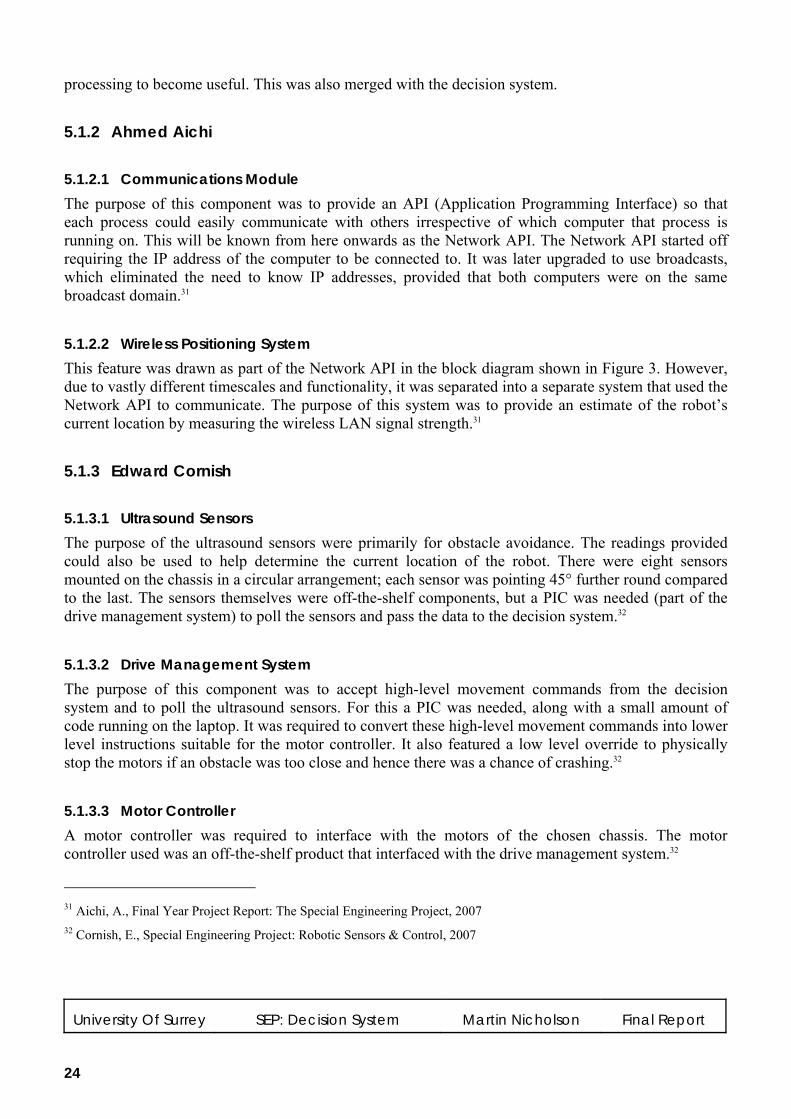
6.6.1 Introduction...................................................................................................................... 40 6.6.2 Corridor Map ................................................................................................................... 40 6.6.3 Dilated Map..................................................................................................................... 41 6.6.4 Distance Map .................................................................................................................. 42 6.6.5 Path Planning Algorithm ................................................................................................ 44 6.6.6 Refining the Map Size..................................................................................................... 45 6.6.7 Improvements Made...................................................................................................... 47 6.6.8 Outstanding Issues .......................................................................................................... 47 6.6.9 Conclusions ...................................................................................................................... 50
6.7 Location Estimation................................................................................................................. 50 6.7.1 Introduction...................................................................................................................... 50 6.7.2 Implementing a Kalman Filter....................................................................................... 50 6.7.3 Emulation Programs........................................................................................................ 52 6.7.4 Testing ............................................................................................................................... 53 6.7.5 Conclusions ...................................................................................................................... 54
6.8 Sensor Fusion ............................................................................................................................ 55 6.8.1 Introduction...................................................................................................................... 55 6.8.2 Expected Sensor Readings............................................................................................ 56 6.8.3 Processing Real Sensor Data......................................................................................... 56 6.8.4 Conclusions ...................................................................................................................... 56

University Of Surrey SEP: Decision System Martin Nicholson Final Report
6
6.9 Movement Commands.......................................................................................................... 60 6.10 Decision System Internal Integration.................................................................................... 60
7. ...Integration Effort.............................................................................................................62
7.1 Autumn Semester.................................................................................................................... 62 7.2 Spring Semester ....................................................................................................................... 63
7.2.1 Decision System and External Image Processing System Communication.......... 63 7.2.2 Easter Holiday Integration Attempt ............................................................................. 63 7.2.3 Sensor Measurements .................................................................................................... 63
8. ...Conclusions....................................................................................................................64
9. ...Discussion .......................................................................................................................65
10. .Future Improvements and Developments...................................................................66
References............................................................................................................................67
Appendices ..........................................................................................................................69
Appendix 1 – Dell Latitude X200 Relevant Specifications............................................................ 69 Appendix 2 – Lynxmotion 4WD3 Robot Chassis Relevant Specifications .................................. 70 Appendix 3 – Computer Sketches of the Designed Platform...................................................... 71

University Of Surrey SEP: Decision System Martin Nicholson Final Report
7
1. Project Introduction
The project is entitled the ‘Special Engineering Project’ (SEP) and at the start was very open. The project description was ‘to build a robot in a team of four’. Although this is a group project, the assessment is individual. Hence each member of the team was set specific tasks that will count as an individual project, but eventually would join together to make a working robot. One of the advantages of this group approach is that a meaningful project can be attempted, with a larger budget, which can be continued by a team next year. Individual projects have a tendency to make limited progress and therefore not to be continued in the future.
The author’s role in the project is the project manager who is responsible for the robot’s decision system. This role includes the overall project management, chairing the weekly meetings, the robot’s path planning, the robot’s location estimation and the integration between the different parts. There are three other members in the team, each doing the following:
• Peter Helland is responsible for both the external and on-board image processing system. The external image processing system will use an existing surveillance system to give an estimated location of the robot. The on-board vision system will use a camera mounted on the robot to provide additional information to the decision system.
• Edward Cornish is responsible for the controlling the motors and obtaining readings from the ultrasound sensors.
• Ahmed Aichi is responsible for providing a means of communication between the different modules of the robot in the form of a Network API and position estimation using wireless LAN signal strength.
This report details the development of the robot’s decision system and mentions the project management. The decision system is the top-level aspect of the robot. The tasks it must accomplish can be roughly broken down into four main components: the planning of paths inside the patrol area, estimating the current location of the robot from noisy estimates, processing the ultrasound sensor readings and issuing movement commands. The project management aspect is also outlined briefly.
Due to the open specification, the first stage was to discuss conceptual ideas of the robot, which is described in section 2 Basic Specification Ideas. The next stage was to define a detailed specification but this required some research beforehand hence section 3 contains some relevant background reading. The detailed robot specification and decisions are given in section 4. The next stage was to split the overall robot into components and for each team member to accomplish the tasks they were assigned. Section 5 discusses this from a project management view point.
The author was assigned the decision system, which is detailed in section 6. Once the individual components were at suitable stages, some integration was attempted. This is outlined in section 7 Integration Effort. Some conclusions are drawn in section 8 and these are followed by some open discussion about the project in section 9. Finally, the report ends with some possible future development ideas in section 10.

University Of Surrey SEP: Decision System Martin Nicholson Final Report
8
2. Basic Specification Ideas
This section outlines some of the ideas, considerations and possible choices at the beginning of the project. There were three basic ideas on which the specification could be built upon.
2.1 Single Intelligent Robot The first idea was a single intelligent robot that would probably integrate a laptop on the chassis, which would allow for image processing, making decisions and communications. This would likely use most, if not all of the budget and the available time. However, if the necessary time and budget were available, relatively simple duplication could result in two or three of these robots. These could interact with each other; the complexity of this interaction depends directly on the time available.
2.2 Multiple Simple Robots The second idea was to make multiple simple robots, each being much less complex than the first idea. They could have some relatively simple rules on how to interact with each other so they could look intelligent. For example simple rules can be applied to each bird in a simulation and when combined into a flock of these birds they will move like a real flock of birds moving and changing direction.
2.3 Single Intelligent Robot with Multiple Simple Robots The final idea involved combining the two previous ideas to have a single complex robot (perhaps simpler than the first idea) with many smaller simple robots. Various ways they could interact were discussed:
• Mother duck, ducklings and nest – the simple robots could run away when fully charged and the intelligent robot has to gather them up again. The mother could either ‘scoop them up’ or emit an audible sound which makes the duckling follow.
• Sheepdog and sheep – the intelligent robot has to herd the simple robots, which would act like the sheep.
• Predator and prey – the intelligent robot has to hunt the simple ones!
2.4 RoboCup RoboCup is an organisation that challenges groups of people to build robots for specific tasks and use them in various challenges against one another. RoboCup @ Home is a relatively new league that focuses on real-world applications and human-machine interaction with autonomous robots. The aim is to develop useful robots that can assist humans in everyday life. Due to this league being new there was the possibility of entering it with a chance of building a competitive effort. However it was decided that if this route was chosen then the specifications would be set and many of the potential choices would be lost. Of the ideas previously stated, only a single intelligent robot would be suitable for entering this competition.1
1 RoboCup@Home, http://www.robocupathome.org/, 2007

University Of Surrey SEP: Decision System Martin Nicholson Final Report
9
2.5 Chosen Idea Initially the decision reached was the final idea being the single intelligent robot with multiple simple robots. This effectively ruled out RoboCup @ Home, but another use was envisioned: having this ‘flock’ of robots on the CVSSP2 corridors, recharging as necessary! Two problems were identified with having small robots roaming the corridors of the CVSSP: firstly the small robots would be too light and weak to open the three sets of fire doors and secondly one of the doors opens in a different direction to the others, which would prevent circular activity.
It was discovered that there is a lack of cheap and small platforms on the market for the ‘flock’. For example a small off the shelf, programmable robot, like the Lego Mindstorms NXT, retails for about £180!3 Therefore the budget does not allow for an off the shelf solution and time constraints do not allow us to custom build multiple robots, while making a large complex one. A lack of mechanical engineers on the team is also a problem hindering a custom made solution. Due to these constraints it was finally decided that the first idea, being a single intelligent robot, would be a better choice. It meant the tasks are easier to spilt, and one robot could be concentrated on, which directly relates to a higher chance of success. If time and budget permits it is possible and planned to simply duplicate it.
Once the choice of the single intelligent robot was made, it was necessary to define some specifications. To do this required some background reading.
2 The CVSSP (Centre for Vision, Speech, and Signal Processing) is the department that Dr. Bowden works for and is
located on the 5th floor of the AB building at Surrey University. Website: http://www.ee.surrey.ac.uk/CVSSP/ 3 Price found on: 03/05/07 at: LEGO Online Store - http://shop.lego.com
University Of Surrey SEP: Decision System Martin Nicholson Final Report
10
3. Background
This section contains some relevant background reading that may be of interest to the reader before reading the rest of the report. It starts off with an introduction to robots and to artificial intelligence. Then a brief case study of an intelligent agent is presented. This case study mentions some sensors and therefore, following this, is a section on sensors, their associated weaknesses and some examples of the problems faced when fusing multiple-sensor data. Then a change of topic occurs into the field of image processing, which is heavily used in this project. Specifically, erosion and dilation are explored. The image processing library used in this project is then discussed. Finally, some of the topics required for filtering noisy estimates are considered. These include: defining the covariance matrix, introducing the Kalman filter, listing some of the filtering libraries available and outlining simultaneous localisation and mapping.
3.1 Introduction to Robots The term robot was first introduced by the Czech playwright Karel Capek in the 1921 play Rosum’s Universal Robots. It comes from the word Robota, which is Czech for ‘forced workers’ in the feudal system. The play featured machines created to simulate human beings in an attempt to prove that God does not exist.4
In 2005 the world market for robots was $6 billion a year for industrial robots, according to the International Federation of Robotics (IFR) and the United Nations Economic Commission for Europe (UNEC). This market is expected to grow substantially; it is predicted that 7 million service robots for personal use (that clean, protect or entertain) will be sold between 2005 and 2008 and 50,000 service robots for professional use will be installed over the same period.5
Jan Karlsson, the author of the UNEC report, cites falling robot prices, an increase in labour costs and improving technology as major driving forces for massive industry investment in robots. There are currently around 21,000 service robots in use worldwide performing tasks such as assisting surgeons, milking cows and handling toxic waste. The report predicts that by the end of 2010 robots will also assist elderly and handicapped people, fight fires, inspect pipes and hazardous sites.6 Robots have the potential for use within the service industries and also as potential carers in our rapidly ageing society.7
Intelligent robots are capable of recognising sounds and images through sensors and analysing this information to determine their actions. Conventional industrial robots (e.g. used in the automotive industry) require work patterns to be input before they can be operated. Large increases in computer power and advances in sensors, control software and mechanics are allowing robots to gain many more abilities, including walking, talking and manipulation. However Artificial Intelligence (AI) is lagging 4 Kittler, J., Machine Intelligence Handout, University Of Surrey, 2007, pages 2-3 5 UNCE, IFR, 2005 World Robotics Survey, Press release ECE/STAT/05/P03, 2005 6 Fowler, J., U.N. sees coming surge in domestic robots, Associated Press, 2004,
http://www.usatoday.com/tech/news/robotics/2004-10-20-robot-report_x.htm 7 RI-MAN revisited, 2006, http://www.pinktentacle.com/2006/03/ri-man-revisited/

University Of Surrey SEP: Decision System Martin Nicholson Final Report
11
behind these developments.8 AI is growing far more sophisticated, drawing on new information on how the human brain works and massive increases in computing power. Business and industry already rely on thousands of AI applications, for example to spot bank fraud and in the development of new drug therapies.9
There are significant problems however, which are hindering the development of robots. For example, different sensors must be used to obtain different kinds of information. There is no one sensor that works flawlessly in all applications. Data fusion techniques are required to utilise the positive side of each sensor, and ignore its negative side. There are still a large number of problems in not only the sensor technology, but also the sensor fusion algorithms.10
To conclude, there are numerous known problems facing the area of robotics; however, in the near future it is an area in which massive development will occur.
3.2 Introduction to Artificial Intelligence Artificial Intelligence (AI) is what happens when a machine does something that could be considered intelligent if a human were to so the same, such as drive a car, play sports or pilot a plane. The term ‘artificial intelligence’ is synonymous to the term ‘machine intelligence’; a machine is by definition something artificial. AI is wired into much of modern society, for example, AI programs are used to spot bank fraud, evaluate mortgage applications and to vacuum floors.9
The term ‘agent’ is used for anything that can be viewed as perceiving its environment through sensors and acting upon that environment through effectors. In AI there are three main types of intelligent agents: firstly the reflex agent, secondly the goal-based agent and finally the utility-based agent. A reflex agent is the simplest type; it perceives its current environment and its actions only depend upon ‘condition-action’ rules. For example: ‘if car in front is breaking then initiate breaking’. A goal based agent is more complicated. It has some perception about the effect its actions will have upon the environment and whether those actions will help towards achieving its long term goal. A utility agent is similar to a goal based agent, but is more complex again, because it has some measure of how successful it is being.11
There are large differences in the environments that intelligent agents operate. Environments are classified as follows:
• Accessible - If an agent's sensors provide access to the complete state of the environment, then the environment is accessible to that agent. An accessible environment means that the robot does not need to maintain an internal model to keep track of the world.
• Deterministic - If the next state of the environment is completely determined by the current 8 Robot special: Almost human, New Scientist Magazine, Issue 2537, 2006, page 38,
http://www.newscientist.com/article.ns?id=mg18925371.800&print=true 9 Boyd, R. S., Machines are Catching Up with Human Intelligence, Knight Ridder Newspapers, 2005 10 Hu, H., Gan, J. Q., Sensors and Data Fusion Algorithms in Mobile Robotics, Report CSM-422, 2005 11 Russell, S., Norvig, P., Artificial Intelligence: A Modern Approach, Prentice Hall, 1995, pages 31-50

University Of Surrey SEP: Decision System Martin Nicholson Final Report
12
state plus the actions selected by the agent, then the environment is deterministic.
• Episodic - In an episodic environment, the agent's experience is divided into ‘episodes’. Each episode consists of the agent perceiving and then acting. Subsequent episodes do not depend upon previous episodes. Episodic environments are simple because the agent does not need to think ahead.
• Static - If the environment cannot change while an agent is deciding on an action, then the environment is static.
• Discrete - If there are a limited number of distinct, clearly defined actions then the environment is discrete.
It is important to understand the environment because different environment types require different agent programs to deal with them effectively.11 The robot built by the special engineering project had the following environment: inaccessible, nondeterministic, non-episodic, dynamic (i.e. not static) and continuous (i.e. not discrete). It was designed to be a goal-based agent.
3.3 Case Study: Stanley The Grand Challenge was launched by the Defence Advanced Research Projects Agency (DARPA) in 2003 to encourage innovation in unmanned ground vehicle navigation. The goal was to develop an autonomous robot capable of crossing unrehearsed off-road terrain. The first competition took place on March 13 2004 and carried a prize of $1M. It required robots to navigate a 142-mile course through the Mojave Desert in no more than 10 hours. 107 teams registered and 15 raced, yet none of the participating robots navigated more than 5% of the entire course. The challenge was repeated on October 8, 2005, with an increased prize of $2M. This time, 195 teams registered, 23 raced and five teams completed the challenge. Stanford University built a robot called ‘Stanley’, which was declared the winner after it finished the course ahead of all other vehicles in 6 hours, 53 minutes, and 58 seconds.12
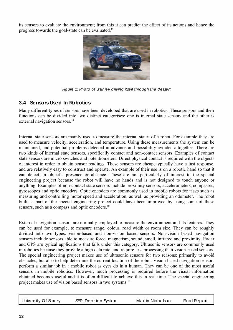
Stanley is a stock Volkswagen Toureg R5 with some modifications carried out by the team including the fitting of skid plates and a reinforced front bumper. A photograph is shown in Figure 1. A custom interface enables direct electronic control of the steering, throttle and brakes. Vehicle data, such as individual wheel speeds and steering angle, are sensed automatically and communicated to the computer system. Stanley has a custom-made roof rack holding nearly all of its sensors. Stanley’s computing system is located in the vehicle’s boot, where special air ducts direct air flow from the vehicle’s air conditioning system. The computing system is in a shock-mounted rack that carries an array of six Pentium M computers and a Gigabit Ethernet switch.12
Stanley is a vastly more complicated robot than what the Special Engineering Project will be attempting. However, it shares the same basic principals of any goal based agent and hence is relevant background reading. The environment and rules are clearly defined by DARPA. The sensors are spilt into two main groups: firstly the environmental sensor group, which includes the roof-mounted lasers, camera & radar system; and secondly the positional sensor group, which includes the inertial measurement devices & GPS systems. These sensors enable perception and analysis of the environment. The effectors include an interface enabling direct electronic control of the steering, throttle and brakes. These sensors and effectors allow Stanley to be classified as an agent. Stanley uses 12 Thrun, S., et al, Stanley: The Robot that Won the DARPA Grand Challenge, Stanford University, 2006, pages 662-669
University Of Surrey SEP: Decision System Martin Nicholson Final Report
13
its sensors to evaluate the environment; from this it can predict the effect of its actions and hence the progress towards the goal-state can be evaluated.12
Figure 1: Photo of Stanley driving itself through the dessert
3.4 Sensors Used In Robotics Many different types of sensors have been developed that are used in robotics. These sensors and their functions can be divided into two distinct categorises: one is internal state sensors and the other is external navigation sensors.10
Internal state sensors are mainly used to measure the internal states of a robot. For example they are used to measure velocity, acceleration, and temperature. Using these measurements the system can be maintained, and potential problems detected in advance and possibility avoided altogether. There are two kinds of internal state sensors, specifically contact and non-contact sensors. Examples of contact state sensors are micro switches and potentiometers. Direct physical contact is required with the objects of interest in order to obtain sensor readings. These sensors are cheap, typically have a fast response, and are relatively easy to construct and operate. An example of their use is on a robotic hand so that it can detect an object’s presence or absence. These are not particularly of interest to the special engineering project because the robot will have no hands and is not designed to touch anyone or anything. Examples of non-contact state sensors include proximity sensors, accelerometers, compasses, gyroscopes and optic encoders. Optic encoders are commonly used in mobile robots for tasks such as measuring and controlling motor speed and acceleration, as well as providing an odometer. The robot built as part of the special engineering project could have been improved by using some of these sensors, such as a compass and optic encoders.10
External navigation sensors are normally employed to measure the environment and its features. They can be used for example, to measure range, colour, road width or room size. They can be roughly divided into two types: vision-based and non-vision based sensors. Non-vision based navigation sensors include sensors able to measure force, magnetism, sound, smell, infrared and proximity. Radar and GPS are typical applications that falls under this category. Ultrasonic sensors are commonly used in robotics because they provide a high data rate, and require less processing than vision-based sensors. The special engineering project makes use of ultrasonic sensors for two reasons: primarily to avoid obstacles, but also to help determine the current location of the robot. Vision based navigation sensors perform a similar job in a mobile robot as eyes do in a human. They can be one of the most useful sensors in mobile robotics. However, much processing is required before the visual information obtained becomes useful and it is often difficult to achieve this in real time. The special engineering project makes use of vision based sensors in two systems.10

University Of Surrey SEP: Decision System Martin Nicholson Final Report
14
3.4.1 Sensor Problems No sensor is perfect. Every sensor has a weakness and is therefore used only for a particular scope. If there were a perfect sensor then multiple sensors per machine would not be required. This statement is also true in humans in the way that one needs multiple senses (e.g. sight, hearing, touch etc) in order to function fully. Two examples of problems are presented here.10
Ultrasonic sensors are active sensors; hence they rely on the reflection of an emitted wave and calculate the distance. However, they often give false range readings caused by irregularities in the surface being reflected off. Algorithms have been developed to help reduce the uncertainty in range readings. One such algorithm is the EERUF (Error Eliminating Rapid Ultrasonic Firing) developed by Borenstein and Koren.13
Cameras are vision based sensors and can be one of the most useful sensors in mobile robotics. However, much processing is required on the pixel data before it becomes useful and it is often difficult to achieve this in real time. Passive vision uses normal ambient lighting conditions and as a result, has to solve problems related to shadows, intensity, colour and texture. Active vision can be used to improve the speed of the image processing by using a form of structured lighting to enhance the area of interest. This results in only the enhanced area needing to be processed. For example, the Sojourner Mars rover used a light striping system for avoiding obstacles. It projected five lines of light strips ahead of the rover which enabled it to detect any obstacles.14
Despite their extra processing requirement, passive vision sensors have been widely used in navigation for various mobile robots. They are often used for landmark recognition, line following, and goal seeking tasks. For example, Saripalli et al enabled the landing of an unmanned helicopter using a passive vision sensor. The system was designed in such a way that the helicopter would update its landing target based on processed vision data. The rest of the landing procedure was achieved using on-board behaviour-based controllers to land on the target with 40cm position error and 7 degrees orientation error.15
3.4.2 Sensor Fusion Examples As described, each different sensor provides different information about the sensed environment. Different sensors will react to different stimuli. Information that can be sensed includes: range, colour, angle and force. Algorithms are required to interpret and process various types of sensor data before it can be used for control and navigation purposes. This has been and will continue to be a challenging task for robotics researchers. This section discusses three sensor fusion examples.10
The satellite based GPS system is often used for localising an outdoor robot, however sometimes the 13 Borenstein, J., Koren, Y., Error Eliminating Rapid Ultrasonic Firing for Mobile Robot Obstacle Avoidance, IEEE
Transactions on Robotics and Automation, Vol. 11, No. 1, 1995, pages 132-138. 14 Sojourner’s Smarts Reflect Latest in Automation, JPL Press Release, 1997 15 Saripalli, S., Montgomery, J. F., Sukhatme, G. S., Visually Guided Landing of an UnmannedAerial Vehicle, IEEE
Transactions on Robotics and Automation, Vol. 19, No. 3, 2003, pages 371-380

University Of Surrey SEP: Decision System Martin Nicholson Final Report
15
position calculated can be inaccurate for a number of reasons. A solution for this was demonstrated by Panzieri et al. Their system integrated, amongst others, inertial sensors with the GPS device. Then a Kalman filter was adopted to fuse the data and reject the noise so that the estimated location uncertainty could be reduced.16
Stanley’s (see 3.3 Case Study: Stanley) laser sensors have a maximum range of 22m, which translates to a maximum safe driving speed of 25mph. This is not fast enough to complete the course in the time allowed. The solution chosen by the team to address this issue was to use a colour camera to increase the range to a maximum of 70m. This method involved comparing the colour of known drivable cells (those within the 22m laser range) to cells outside of the laser range. If the colour was similar enough and there was a continuous path then it was assumed that this was still drivable road. This assumption allowed cells to be labelled as drivable, despite not having exact knowledge. This is obviously a compromise and would not work in all situations and environments. For example, in urban areas the colour of the pavement is similar to that of the road. This algorithm is self learning as it refines future estimates based upon the laser information gathered when it reaches the predicted regions.12
Estimating vehicle state is a key prerequisite for precision driving. Inaccurate pose estimation can cause the vehicle to drive outside boundaries, or build terrain maps that do not reflect the state of the robot’s environment, leading to poor driving decisions. In Stanley, the vehicle state comprised a total of 15 variables. A Kalman filter was used to incorporate observations from the GPS, the GPS compass, the inertial measurement unit, and the wheel encoders. The GPS system provided both absolute position and velocity measurements, which were both incorporated into the Kalman filter. The Kalman filter was used to determine the vehicle’s coordinates, orientation, and velocity.12
3.5 Erosion and Dilation of Binary Images Erosion and dilation are fundamentally neighbour operations to process binary images. Because the values of pixels in the binary images are restricted to 0 or 1, the operations are simpler and usually involve counting rather than sorting or weighted multiplication and addition. Operations can be described simply in terms of adding or removing pixels from the binary image according to certain rules, which depend on the pattern of neighbouring pixels. Each operation is performed on each pixel in the original image using the original pattern of pixels. None of the new pixel values are used in evaluating the neighbour pattern.17
Erosion removes pixels from features in an image or, equivalently, turns pixels OFF that were originally ON. The purpose is usually to remove pixels that should not be there. The simplest example is pixels that fall into the brightness range of interest, but do not lie within large regions with that brightness. Instead, they may have that brightness value either accidentally, because of finite noise in the image, or because they happen to straddle a boundary between a lighter and darker region and thus have an averaged brightness that happens to lie in the range of interest. Such pixels cannot be distinguished because their brightness value is the same as that of the desired regions.17
16 Panzieri, S., Pascucci, F., Ulivi, G., An Outdoor Navigation System using GPS and Inertial Platform, IEEE/ASME
Transactions on Mechatronics, Vol. 7, No. 2, 2002, pages 134-142 17 RUSS, C. J., Image Processing Handbook, 4th Edition, CRC Press, 2002, pages 409-412
University Of Surrey SEP: Decision System Martin Nicholson Final Report
16
The simplest kind of erosion, sometimes referred to as classical erosion is to remove (set to OFF) any pixel touching another pixel that is part of the background (is already OFF). This removes a layer of pixels from around the periphery of all features and regions, which will cause some shrinking of dimensions. Erosion can entirely remove extraneous pixels representing point noise or line defects because these defects are normally only a single pixel wide.17
Instead of removing pixels from features, a complementary operation known as dilation (or sometimes dilatation) can be used to add pixels. The classical dilation rule, analogous to that for erosion, is to add (set to ON) any background pixel which touches another pixel that is already part of a foreground region. This will add a layer of pixels around the periphery of all features and regions, which will cause some increase in dimensions and may cause features to merge. It also fills in small holes within features. Because erosion and dilation cause a reduction or increase in the size of regions respectively they are sometimes known as etching and plating or shrinking and growing.17
Erosion and dilation respectively shrink and expand an image object. However, they are not inverses of each other. That is, these transformations are not information preserving. A dilation after an erosion will not necessarily return the image to its original state nor will an erosion of a dilated object necessarily restore the original object.18 For example, following an erosion with a dilation will more or less restore the pixels around the feature periphery, so that the dimensions are (approximately) restored. Isolated pixels that have been completely removed however, do not cause any new pixels to be added. They have been permanently erased from the image.17
This loss of information from these two operations one after the other, provide the basis for the definition of another pair of morphological transformations called morphological opening and closing.18 The combination of an erosion followed by a dilation is called an opening, referring to the ability of this combination to open up gaps between just-touching features. It is one of the most commonly used sequences for removing pixel noise from binary images. Performing the same operations in the opposite order (dilation followed by erosion) produces a different result. This sequence is called a closing because it can close breaks in features. Several parameters can be used to adjust erosion and dilation operations, particularly the neighbour pattern and the number of iterations. In most opening operations, these are kept the same for both the erosion and the dilation.17
3.6 The CImg Library The Cool Image (CImg) library is an image processing library for C++. It is a large single header file, which provides the ability to load, save, process and display images. It is portable, efficient and relatively simple to use. It compiles on many platforms including: Unix/X11, Windows, MacOS X and FreeBSD.19
It being comprised of a single header file is a unique feature of the CImg Library. This approach has many benefits. For example, no pre-compilation is needed because all compilation is done with the rest 18 Plataniotis, K. N., Venetsanoupoulos, A. N., Color Image Processing and Applications, Springer-Verlag Berlin and
Heidelberg GmbH & Co. KG, 2000, pages 149-152 19 Tschumperlé, D., The CImg Library Reference Manual, Revision 1.1.7, 2006, Pages 1-2

University Of Surrey SEP: Decision System Martin Nicholson Final Report
17
of the code. There are no complex dependencies that have to be handled. This approach also leads to compact code because only CImg functions used are compiled and appear in the executable program. The performance of the compiled program is also improved because the class members and functions are all inline.19
3.7 Covariance Matrix The covariance of two variables can be defined as their tendency to vary together. The resulting covariance value will be larger than 0 if two variables tend to increase together, below 0 if they tend to decrease together and 0 if they are independent.20 A covariance matrix is a collection of many covariances in the form of a matrix.21
3.8 Kalman Filters The Kalman filter was developed 40 years ago by Kalman, R. E. It is systematic approach to linear filtering based on the method of least-squares. With the exception of the fast Fourier transform, the Kalman filter is probably the most important algorithmic technique ever devised.22
The Kalman filter is a recursive filter which has two distinct cycles. It can estimate the state of a dynamic system from noisy measurements.23 The Kalman filter estimates the state at a time step and then obtains feedback in the form of a noisy measurement. Therefore there are two distinct groups of equations for the Kalman filter: ‘predict’ equations and ‘update’ equations. The ‘predict’ equations project the current state and error covariance forward in time to obtain a prior estimate for the next time step. The ‘update’ equations use a measurement to provide the feedback; they merge the new measurement with the prior estimate to obtain an improved estimate. This is an ongoing continuous cycle as shown in Figure 2. The Kalman filter bases its prediction on all of the past measurements.24
Figure 2: The Kalman filter cycle. The ‘Predict’ part of the cycle estimates the next sate. The ‘Update’
part of the cycle adjusts that estimate using a measurement given at that time step.24
20 Weisstein, E. W., Covariance, MathWorld, http://mathworld.wolfram.com/Covariance.html, 2006 21 Weisstein, E. W., Covariance Matrix, MathWorld, http://mathworld.wolfram.com/CovarianceMatrix.html, 2006 22 Zarchan, P., Howard, M., Fundamentals of Kalman Filtering: A Practical Approach, Second Edition, American Institute
of Aeronautics and Astronautics Inc, 2005, Pages xvii - xxiii 23 Kalman filter, Wikipedia, http://en.wikipedia.org/wiki/Kalman_filter, 2007 24 Welch, G., Bishop, G., An Introduction to the Kalman Filter, 2006, pages 2-7

University Of Surrey SEP: Decision System Martin Nicholson Final Report
18
An example of its use is in a radar application used to track a target. Noisy measurements are made that contain some information about the location, the speed, and the acceleration of the target. The Kalman filter removes the effects of the noise by exploiting the dynamics of the target. It can estimate the location of the target at the present time (filtering), at a future time (prediction), or at a time in the past (interpolation or smoothing).23
3.9 Filtering Libraries Available for C++ Currently, there is not a standard numerical or stochastic library for C++ available, such as the Standard Template Library (STL). Therefore, as one would expect there are a wide range of libraries available providing the necessary functionality. Some of them are outlined in this section.
3.9.1 Bayes++ Bayes++ is an open source C++ library implementing several Bayesian Filters. Bayes++ implements many filtering schemes for both linear and non-linear systems. It includes, amongst others, a range of different Kalman Filters. It can be used for a wide range of purposes including SLAM (see 3.10 SLAM). Bayes++ uses the Boost libraries25 and compiles on both Linux and Windows. Boost is used by Bayes++ to provide linear algebra, compiler independence, and a common build system.26
The author’s opinion subsequent to trying Bayes++ is that it suffers from a lack of documentation and a tedious installation. This made attempting to use it tricky. Furthermore, there is not an active community and the latest release is dated 200327.
3.9.2 The Bayesian Filtering Library (BFL) The BFL is an open source C++ library with support for several Particle Filter algorithms. It has been designed to provide a fully Bayesian software framework and is not limited to a particular application. This means both its interface and implementation are decoupled from particular sensors, assumptions and algorithms that are specific to a certain applications.28
3.9.3 OpenCV OpenCV stands for Open Source Computer Vision Library and was developed originally by Intel. It is a collection of functions and classes that implement many Image Processing and Computer Vision algorithms. OpenCV is a multi-platform API written in ANSI C and C++, hence is able to run on both Linux and Windows. OpenCV includes a basic Kalman Filter. There is a large amount of documentation available for OpenCV as well as an active user community.29
OpenCV was crucial to Stanley’s (see 3.3 Case Study: Stanley) vision system.12
25 Boost peer-reviewed portable C++ libraries, http://www.boost.org/, 2007 26 Stevens, M., Bayes++: Open Source Bayesian filtering classes, http://bayesclasses.sourceforge.net/, 2003 27 Checked: http://sourceforge.net/projects/bayesclasses/, On: 03/05/07 28 The Bayesian Filtering Library (BFL), http://www.orocos.org/bfl, 2007 29 OpenCV Documentation, Contained within: OpenCV_1.0.exe, 2006

University Of Surrey SEP: Decision System Martin Nicholson Final Report
19
3.10 SLAM SLAM stands for Simultaneous Localisation and Mapping. It is a process used by robots when introduced to a new environment – the robot must build a map of the surrounds and where it is in relation to identified landmarks. SLAM allows an autonomous vehicle to be in an unknown location in an unknown environment and build a map, using only relative observations of the environment. This map is also simultaneously used for navigational purposes. If a robot could do this then it would make such a robot ‘autonomous’. Thus the main advantage of SLAM is that it eliminates the need for artificial infrastructures or a prior knowledge of the environment.30
The general SLAM problem has been the subject of substantial research since the beginning of a robotics research community and even before this, in areas such as manned vehicle navigation systems and geophysical surveying. A number of approaches have been proposed to accomplish SLAM, as well as more simplified navigational problems where prior map information is made available. The most widely used approach is that of the Kalman filter. SLAM is far from a perfected art: it still requires further development.30
The special engineering project is not concerned with SLAM because the robot will be travelling in a known area and hence a prior map can be defined.
30 Gamini Dissanayake, M. W. M., A Solution to the Simultaneous Localization and Map Building (SLAM) Problem, IEEE
Transactions on Robotics and Automation, Vol. 17, No. 3, 2001, pages 229-241

University Of Surrey SEP: Decision System Martin Nicholson Final Report
20
4. Full Specification Decisions
Once some research had been carried out, the next stage was to define the robot’s specification and hence its purpose. The team had to choose a chassis and a laptop which is detailed next. A choice of which operating system to use on the laptop also existed. There were some projects running in parallel that needed considering. Afterwards these choices and considerations a final specification was agreed.
4.1 Choosing the Chassis and Laptop It was decided that a custom made chassis was not really an option; therefore various off-the-shelf chassis options were researched. The plan was to use a laptop on the chassis as the robot’s brain because it can run readily available, standard software and provides significant processing power. Of the available chassis options the maximum payload was 2.3kg, which confined us to an ‘ultra portable’ laptop. The budget however, would barely allow for one of these, let alone two. Therefore two CVSSP laptops (Dell Latitude X200) were provided; they are ‘ultra portable,’ weighing about 1.3kg. They are not particularly new, but have adequate processing power for the intended use. Full specifications can be found in Appendix 1 – Dell Latitude X200 Relevant Specifications.
After examining the chassis available on the market, the Lynxmotion 4WD3 was a relatively simple choice. It is physically big enough to carry the required laptop and it can carry the 1.3kg mass of the laptop, along with the rest of the payload. It makes use of four motors and requires a dual channel motor controller separating the front and back motors. Full specifications can be found in Appendix 2 – Lynxmotion 4WD3 Robot Chassis Relevant Specifications. An extra frame can be mounted on this chassis suitable for fixing the laptop to.
4.2 Windows versus Linux Linux has many advantages over Windows, cost not really being one for this project, due to academic licences. Linux can be customised to a far greater degree. For example to save resources no GUI (Graphical User Interface) has to be installed; this also would benefit the sending of commands and the receiving of status information because only text would have to be transmitted. However, a webcam is to be used and due to many webcam manufacturers using propriety compression algorithms while not producing Linux drivers, the chances of finding Linux support for a given webcam is low. As a result the consensus is that Windows is the best option for the on-board laptop.
4.3 Parallel Projects Dr Bowden has two projects running separately which are related to the special engineering project and had the possibility of being included in the final robot.
The first is by Thomas Thorne and it aims to make an animated face, which can be rendered and shown on the laptop screen. Instead of trying to make this face look human, which would result in a fake looking face due to the difficulties in making an animated face look real, it will be made out of particles to give it a unique effect. This face would be capable of showing emotions and would give the robot an impressive interface.

University Of Surrey SEP: Decision System Martin Nicholson Final Report
21
The second is by Olusegun Oshin and it aims to be able to control two Logitech QuickCam Sphere cameras (pictured in Figure 10). These cameras feature motorised pan and tilt and a stand. Using two of these on the robot could make it look as if it has moving ‘bug eyes’. This would add a massive ‘wow factor’ to the robot as well as adding extra (independently moving) cameras to the image processing system, which could then give more information to the decision system.
4.4 Final Robot Specification It was decided that the robot would consist of a laptop on top of a chassis. The laptop was provided and the chassis was chosen in section 4.1. A frame needed to be built to hold the laptop and be mounted on top of the chassis; this is described in 5.5 Chassis Frame Design. This robot would patrol the CVSSP2 corridors and the external image processing system would identify people walking the corridors, prioritise them and send co-ordinates to the robot so it could greet them. This gave the robot an aim and when there are no people about, locations can be picked at random for the robot to visit.
A block diagram, shown in Figure 3, was drawn to illustrate how the robot would be split up into components, and how these components would interact. Brief details of all the components, including who they were assigned to, are described in section 5.1 Team Management. Figure 3 shows which components need to be built by the team and which are off the shelf.
To achieve this aim the external image processing system has to be able to track people and send the relevant coordinates to the decision system (running on the laptop). All communication will take place through the Network API. The external image processing system will also send an estimate of the robot’s location, as well as updates as to where the people are currently if they are moving. The decision system must then use this information to try to get to the location of the people using its sensors to guide it and using the drive management system for movement. There will be various estimates (each with an uncertainty) of the robot’s location from the different systems. These must be fused together by the decision system to produce an overall estimate of the robot’s location.
Potentially the animated face could make the robot look as though it is talking to people. The ultimate goal would have been for it to be able to greet people and accept some voice commands.

University Of Surrey SEP: Decision System Martin Nicholson Final Report
22
Figure 3: The initial block diagram showing the components/sub-systems of the robot.

University Of Surrey SEP: Decision System Martin Nicholson Final Report
23
5. Project Management
As previously stated the author was responsible for the overall project management, as well as contributing the decision system to the project. This section details some aspects of the project management that took place. The project management started with spitting the overall task of building a robot into smaller sub-systems. These sub-systems were then assigned to the appropriate team members. This is covered under 5.1 Team Management. Then the timing of the project had to be planned so that team members knew about the deadlines involved. This is outlined in section 5.2 Time Management; the timing had to be monitored and revised during the course of the project. There are two remaining items that required constant attention throughout the project. The first was the management of the group budget, which is detailed in section 5.3. The second was the organisation and chairing of the weekly meetings, which is outlined in section 5.4. There was an extra one-off task to build the robot’s flat-pack chassis and design the frame. This is detailed in section 5.5 Chassis Frame Design. Finally, the success of the project is evaluated in section 5.6.
5.1 Team Management The first task, once the purpose and specifications of the robot had been discussed, was to split the robot into components/sub-systems. These components had to be treated as separate projects for the purposes of allocating project marks. Each team member entered the special engineering project with a particular job description. Once the system block diagram (Figure 3) had been agreed, it was necessary to assign the components to the relevant team members. Many of these components were assigned by default to team members due to their job description. This section details each team member and the tasks assigned to them. Some extra tasks and components were identified and allocated subsequently to the drawing of the block diagram shown in Figure 3.
5.1.1 Martin Nicholson
5.1.1.1 Location System The purpose of the location system was to determine the robot’s current location and find a path to a destination. It was originally intended to be separate from the decision system, but instead became a part of it.
5.1.1.2 Decision System The purpose of the decision system was to use the information provided by all the other sub-systems to make decisions about what the robot would do - the ‘brain’ of the robot. It is the top-level system because it integrates with virtually every other system. It was decided that the decision system would be merged with the location system as they have dependence on one another. The decision system will take multiple inputs, determine its current location, have a destination suggested to it and send the necessary drive management instructions in order to get there. The design of the decision system is discussed in section 6.
5.1.1.3 Sensor Fusion This was identified subsequently to the drawing of the component diagram. The sensor readings coming from the drive management system were sent as unprocessed values and hence needed
University Of Surrey SEP: Decision System Martin Nicholson Final Report
24
processing to become useful. This was also merged with the decision system.
5.1.2 Ahmed Aichi
5.1.2.1 Communications Module The purpose of this component was to provide an API (Application Programming Interface) so that each process could easily communicate with others irrespective of which computer that process is running on. This will be known from here onwards as the Network API. The Network API started off requiring the IP address of the computer to be connected to. It was later upgraded to use broadcasts, which eliminated the need to know IP addresses, provided that both computers were on the same broadcast domain.31
5.1.2.2 Wireless Positioning System This feature was drawn as part of the Network API in the block diagram shown in Figure 3. However, due to vastly different timescales and functionality, it was separated into a separate system that used the Network API to communicate. The purpose of this system was to provide an estimate of the robot’s current location by measuring the wireless LAN signal strength.31
5.1.3 Edward Cornish
5.1.3.1 Ultrasound Sensors The purpose of the ultrasound sensors were primarily for obstacle avoidance. The readings provided could also be used to help determine the current location of the robot. There were eight sensors mounted on the chassis in a circular arrangement; each sensor was pointing 45° further round compared to the last. The sensors themselves were off-the-shelf components, but a PIC was needed (part of the drive management system) to poll the sensors and pass the data to the decision system.32
5.1.3.2 Drive Management System The purpose of this component was to accept high-level movement commands from the decision system and to poll the ultrasound sensors. For this a PIC was needed, along with a small amount of code running on the laptop. It was required to convert these high-level movement commands into lower level instructions suitable for the motor controller. It also featured a low level override to physically stop the motors if an obstacle was too close and hence there was a chance of crashing.32
5.1.3.3 Motor Controller A motor controller was required to interface with the motors of the chosen chassis. The motor controller used was an off-the-shelf product that interfaced with the drive management system.32
31 Aichi, A., Final Year Project Report: The Special Engineering Project, 2007 32 Cornish, E., Special Engineering Project: Robotic Sensors & Control, 2007

University Of Surrey SEP: Decision System Martin Nicholson Final Report
25
5.1.4 Peter Helland
5.1.4.1 On-Board Image Processing System The purpose of this component was to use an on-board webcam to provide the decision system with an estimate of the movement occurred. It was able to determine how fast the robot was moving and whether or not any turning motion was detected.33
5.1.4.2 External Image Processing System There was an existing surveillance system fitted in the CVSSP2 corridors. The purpose of the external image processing system was to estimate the robot’s current location and to identify human activity. The current location estimate was to be sent to the decision system along with the destination co-ordinates of the identified human activity. If no human activity could be found then it would send random co-ordinates for the robot to visit.33
5.1.5 Unassigned Components These were components that were considered ‘luxury items’ and hence were not assigned unless a team member had some spare time. Neither was built due to a lack of time.
5.1.5.1 Power Management and Main Battery It would have been useful to have a power management system which could pass the decision system information on the current state of the main battery. It would have also been useful to have had the ability for the robot to recharge itself. This would have involved some form of docking station that, when required, the robot could drive into and recharge itself.
5.1.5.2 Pedometer It would have been useful to have some form of odometer device so that the distance travelled by the robot could have been measured. A pedometer would have been more accurate than relying upon how far the motors were supposed to move the robot.
5.2 Time Management This section details a brief overview of the time management that took place for the team as a whole. A diary style approach has been avoided as much as possible and hence only key events or examples have been noted.
Once the system components had been assigned to the relevant people the next step was to instruct the team members to make an individual Gantt chart for the tasks assigned to them. These Gantt charts were only approximate because it was an initial plan and no team member could predict exactly what was involved in their task. Nevertheless, an overall team Gantt chart was made based upon these individual Gantt charts. This Gantt chart features abstraction for increased clarity and is shown in Figure 4. There are different colours associated with different team members as shown in the key.
33 Helland, P., Special Engineering Project: Visual System, 2007

University Of Surrey SEP: Decision System Martin Nicholson Final Report
26
It includes the autumn semester, the spring semester, as well as the Christmas holidays. There is a greyed out region on weeks 14 and 15 in the autumn semester to allow for exams and the associated revision. The second week of the Christmas holidays is deliberately blank because that is where Christmas lies. It shows the systems in the broadest sense and for further detail the individual Gantt charts was consulted. From the very beginning time was going to be tight. The first half of the autumn semester was mainly spend deciding upon the specifications and each team member getting familiar with their project area.
During the course of the first semester some aspects had been achieved early such as making a local map and choosing the interfacing decisions for the different systems. However, all of the team was behind schedule. By the end of the autumn semester:
• Martin Nicholson (author) had created the map early, agreed interfacing decisions and had created a mapping algorithm that worked some of the time but was falling behind in terms of researching data fusion techniques and creating test input files.
• Ahmed Aichi had delivered a working Network API by the end of the semester but the learning of C++ had caused delays and hence the wireless positioning system had made little progress.
• Edward Cornish had achieved some control of the motors, but was behind in other aspects such as interfacing with the chosen sensors and coding the PIC.
• Peter Helland was able to process the optical flow to obtain crude estimates and had started coding the external image processing system but was also behind schedule.
The first integration attempt was scheduled for the end of the autumn semester because none of the team members were ready beforehand. This delay caused a delay in the writing of the interim report, which meant that each team member had to accomplish this during the Christmas holidays. This had a knock-on effect in the way that less project work was carried out over the Christmas holidays than planned. This caused further delays.
By the first week back in the spring semester the team were made aware of the delays. It was agreed that it was still potentially possible to produce a working robot. There was optimism and enthusiasm amongst the team. Each team member continued to work towards the goal. By week 4 it was clear that the Gantt chart needed revising to reflect the various changes and delays. This revised Gantt chart started in week 6 and is shown in Figure 5. It was drawn solely by the author and agreed by the rest of the team. It is more meaningful than the last one due to a more up-to-date knowledge of the project. The previous Gantt chart relied on estimates and assumptions, whereas by this time everyone knew clearly what had to be done and roughly how to achieve it.
When updating the Gantt chart the final dissertation deadline was known to be in week 13 of the spring semester – the exact day was not known however. This meant that this Gantt chart continued into the Easter holidays and the first three weeks back. It was known for sure that exams lay after Easter, in weeks 11 to 15. An estimate was based upon last year’s exam timetable34. Most of the level 3 exams lay 34 Examination Timetable, Spring Semester, Session 2005/06,
http://www.ee.surrey.ac.uk/Teaching/Exams/ExamTimetable.pdf , 2006

University Of Surrey SEP: Decision System Martin Nicholson Final Report
27
in weeks 12 and 13, so it was assumed that there would be some time for integration attempts in weeks 11 and maybe even 12. This can be seen on the revised Gantt chart. However, when the exam timetables were released it turned out that this year, the exams had been shifted a week earlier than last year, with all of the exams being in week 12.35 This meant that time after Easter was scarce and barely existent.
The revised Gantt chart shown in Figure 5 featured many tight schedules. Some of these were met, some of them were not. For example, in week 8 Edward Cornish was having some stability issues with the PIC, which were causing delays but had already looked into a compass device.
The aim was to get each individual component finished by the end of the Easter holidays, and integrate it in weeks 11 and 12. However, as already explained there was very little time in weeks 11 and 12. Therefore an integration attempt was scheduled during the Easter holidays instead. This is further discussed in 7.2.2 Easter Holiday Integration Attempt. The aim was to remote control the robot around the corridors while receiving estimates of its location from the wireless positioning system and the external image processing system. From these estimates the decision system could estimate a location and display it on the map. However, due to delays in the individual system’s functioning, the integration was not successful. This was because the wireless positioning system could not be used during the day time for fears of service interruption for other users and because the external image processing system was not ready. Clearly this meant that this revised plan had also slipped.
In week 11 of the spring semester there was some integration attempted (see section 7.2.3) but there was no real team plan because each team member had exams to prepare for, a dissertation to write and some final changes to perform on their component of the system. Hence week 11 was the final week that any form of group meeting took place.
To conclude, the author would like to state that good time management was attempted but deadlines kept being postponed. Much of this was outside of the author’s control.
35 Department of Electronic Engineering Examination Timetable, Spring Semester, Session 2006/07,
http://www.ee.surrey.ac.uk/Teaching/Exams/spring07.xls, 2007

University Of Surrey SEP: Decision System Martin Nicholson Final Report
28
Figure 4: The initial combined team Gantt chart. There are different colours associated with different
team members as shown by the key. The blue ‘Joint’ bars have the first letter of the name of the
individuals involved.
Figure 5: The revised group Gantt chart. There are different colours associated with different team
members as shown by the key. The Integration attempts were planned to occur every two weeks so
that the work achieved could be integrated with the other systems.

University Of Surrey SEP: Decision System Martin Nicholson Final Report
29
5.3 Budget Management Due to the special engineering project being a group project the budget is higher than that of a normal project. The budget given to the team was £1000, with purchase values having to be included with VAT. This section details some of the decisions made about the spending of the budget. The budget had to be continually monitored and used wisely because of the relative ease of spending £1000 on robotic equipment.
The budget was insufficient for a ‘flock’ of small robots due to relatively high costs for each one. The budget also did not allow for the purchase of two ultra-portable laptops. Therefore the idea was changed to have two bigger robots, using existing provided laptops. This was explained in 2.5 Chosen Idea. The webcams used for the on-board vision system are also existing equipment. Figure 6 shows the items and costs that have been purchased throughout the course of the project. Currently the budget remaining is £42.16 minus any minor postage charges that were not available at the time of order.
Figure 6 clearly shows what has been ordered. It is spilt into sections by a blank line between them. The sections are generally related but follow in no particular order. The following is a brief description of each section:
• The highest cost was the chassis and the motor controller, so only one of each was been ordered at the start so that suitability tests could be performed.
• Once the chassis and the motor controller had been tested then one more of each was ordered in the spring semester so the robot could be duplicated.
• The provided laptops do not have any USB 2.0 sockets, which are needed for the webcam. Therefore two USB 2.0 CardBus adapters were purchased. The ball & socket heads fix the webcam to the chassis. They were ordered separately in case of an error or a change in the webcam used.
• The main battery to power the motors was better value in a double pack and was ordered along with a suitable charger. Both robots shared the same charger and had a battery each.
• Two ultrasound rangers were purchased initially so that suitability tests could be performed before buying larger numbers. Once they had been accepted then 14 more were ordered. The motors and sensors use an I²C bus so two USB converters were ordered. The USB 2.0 hub was ordered so that Edward Cornish could test the sensors and other related 5V circuitry without using a laptop. This was to reduce the risk of somehow damaging the provided laptop. Three PIC chips were ordered, due to their low cost, in case one should become damaged in the experimentation phase. It turned out that all three were faulty, so another batch of three was ordered. Thee oscillators were ordered for use with the PIC chips. The USB sockets were ordered so that the sensor circuitry could use the power provided by a USB port. Finally, a PCB was designed and two were ordered.
• The wireless positioning system required three wireless access points in order to obtain accurate results. Two were ordered and the other was temporarily sourced from the author.
• Of the two existing laptops batteries, one had a good battery life (≈1.5 hours) and the other one had a terrible battery life (≈0.4 hours). Therefore a replacement battery was needed.
• Finally, in order to neaten the connections to the PCB, some connectors were required.

University Of Surrey SEP: Decision System Martin Nicholson Final Report
30
The initial cost per robot was originally estimated at £415.76 (using the existing laptop and webcam). This increased slightly to £433.83, which is shown in Figure 7. This is a small increase and so represents a good initial estimate. This figure includes a charger for each robot, which was unnecessary as they can share one. It does not include items that were not incorporated into the robot such as the USB 2.0 Hub, the wireless access points, the duplicate PIC chips, oscillators and USB sockets. It also does not include the new laptop battery because that would not have been required in all circumstances – it was just unfortunate that one of the existing laptop batteries was useless.
To conclude, the group managed to build the robots within the given budget. This was largely down to the fact that some existing equipment could be used, and partly due to careful budget use by the team.

University Of Surrey SEP: Decision System Martin Nicholson Final Report
31
Item Quantity Cost Each Total Cost Total Cost (inc VAT)
Motor controller - MD22 1 £39.99 £39.99 £46.99
Chassis with motors - 4WD3 1 £135.42 £135.42 £159.12
Motor controller - MD22 (2) 1 £39.99 £39.99 £46.99
Chassis with motors - 4WD3 (2) 1 £135.42 £135.42 £159.12
USB 2.0 Cardbus Adapter 2 £11.40 £22.80 £26.79
Hama Ball & Socket Head 38mm 1 £7.65 £7.65 £8.99
Hama Ball & Socket Head 38mm (2) 1 £7.64 £7.64 £8.98
Pro-Peak 2500 AC/DC Charger 1 £25.52 £25.52 £29.99
7.2V 3600mAh Ni-MH Battery (2 Pack) 1 £38.30 £38.30 £45.00
Ultrasound Ranger - SRF05 2 £11.49 £22.98 £27.00
Ultrasound Ranger - SRF05 14 £11.49 £160.86 £189.01
USB to I2C interface - USB/I2C 2 £16.56 £33.12 £38.92
USB 2.0 4-Port Powered Hub 1 £16.99 £16.99 £19.96
PIC18f2220 Micro Controller 3 £3.95 £11.85 £13.92
PIC18f2220 Micro Controller (2) 3 £3.88 £11.64 £13.68
25MHz Crystal Oscillators 3 £1.95 £5.85 £6.87
USB Type B Socket 3 £0.33 £0.99 £1.16
PCBs 2 £0.88 £1.75 £2.06
D-Link DWL-700AP 1 £18.30 £18.30 £21.50
D-Link DWL-700AP (2) 1 £17.45 £17.45 £20.50
Dell Latitude X200 3900mAh Battery 1 £46.17 £46.17 £54.25
PCB connectors for sensors and I2C
interface 1 £14.50 £14.50 £17.04
Total £815.18 £957.84
Figure 6: List and cost of all items purchased throughout the project. The figures have been spilt into
related sections but in no particular order.

University Of Surrey SEP: Decision System Martin Nicholson Final Report
32
Item Quantity Cost Each Total Cost Total Cost (inc VAT)
Ultrasound Ranger - SRF05 8 £11.49 £91.92 £108.01
USB to I2C interface - USB/I2C 1 £16.56 £16.56 £19.46
Chassis with motors - 4WD3 1 £135.42 £135.42 £159.12
Motor controller - MD22 1 £39.99 £39.99 £46.99
USB 2.0 Cardbus Adapter 1 £11.40 £11.40 £13.40
PIC18f2220 Micro Controller 1 £3.95 £3.95 £4.64
25MHz Crystal Oscillators 1 £1.95 £1.95 £2.29
USB Type B Socket 1 £0.33 £0.33 £0.39
Hama Ball & Socket Head 38mm 1 £7.65 £7.65 £8.99
Pro-Peak 2500 AC/DC Charger 1 £25.52 £25.52 £29.99
7.2V 3600mAh Ni-MH Battery (2 Pack) 0.5 £38.30 £19.15 £22.50
PCB connectors for sensors and I2C
interface 1 £14.50 £14.50 £17.04
PCB 1 £0.88 £0.88 £1.03
Total £369.22 £433.83
Figure 7: The total cost per robot. This figure only includes the essentials to build the robot. It does not
include any items that were ordered but not attached to the robot.
5.4 Chairing the Weekly Meetings Another task that required constant attention was the chairing of the weekly meetings. Each week a meeting had to be organised in which the project progress could be evaluated. To accomplish this, a firm meeting structure was set up and adhered to. The team had to email any topics they wanted raising at a meeting before the agenda was sent out. The agenda was sent out at least two days in advance of the meeting. The meetings had a common structure and only allowed a small amount of time for the ‘any other business’ section to make them efficient. Minutes were taken by each team member in a round robin style. These minutes were always sent within five days of the meeting. Any actions identified during the meeting were assigned to a specific team member and included in the minutes. At the beginning of each meeting, the statuses of the actions from the last meeting were checked. Each action would either be carried over to the next week or marked as complete. This meant that actions would not be forgotten about.
5.5 Chassis Frame Design There was a one-off task to build the chosen chassis and design a frame to sit on top of it. The chosen chassis is the Lynxmotion 4WD3 and its specifications are included in Appendix 2 – Lynxmotion 4WD3 Robot Chassis Relevant Specifications for reference. This task was carried out equally by the author and Edward Cornish.
The Lynxmotion 4WD3 arrived as a flat pack, therefore the first task was to assemble it. The included

University Of Surrey SEP: Decision System Martin Nicholson Final Report
33
instructions were helpful and the lab had all the necessary tools. Once put together it was connected to a 7.2v DC power supply and tested without the motor controller. All the four motors worked and hence the wheels turned. The chassis after assembly was photographed and is shown in Figure 8. The laptop used is a Dell Latitude X200 of which further specifications are included in Appendix 1 – Dell Latitude X200 Relevant Specifications for reference. To demonstrate the good size of the laptop compared to the size of the chassis, a photograph was taken with the laptop on top of the chassis and this is shown in Figure 9.
The next task was to design a frame to bolt onto the chassis that would hold a laptop, the camera(s) and all the sensors. The workshop staff were able to help with key aspects of the design, including the materials to be used. It was decided that the design would need to be finalised and requested as soon as possible because it is likely to be time consuming for the workshop. If it were left until after the Christmas holidays then it would probably have be delayed by other projects. The design was meant to be very open to make it easier for the workshop to improvise and construct it using the most efficient techniques. The laptop, a sensor and the robot chassis were loaned to the workshop so this was possible. The author and Edward Cornish developed some sketches to help explain ideas to the workshop staff. Two of these platforms were ordered so that the robot could be duplicated.
The key design requirements of this platform were:
• It had to be lightweight, but sturdy.
• It had to take up to 8 ultrasound sensors at the points of a compass.
• It had to hold the laptop safely in place, even during a collision. It had to be designed so that it would not block any of the laptop ports or cooling vents.
• It had to hold the screen open at a fixed angle. There is a project running in parallel to animate a face, which may be shown on this screen (see 4.3 Parallel Projects).
• It had to have a fixing for the main camera used for the on-board image processing. This needed to be sturdy to reduce any camera wobbling. The chosen webcam used a standard 38mm fixing screw, so was is possible to drill a hole in the frame and use a standard 38mm Ball & Socket Head to mount it. This had the advantage that the camera could be moved to the correct angle and then locked into position.
• It had to be able to carry two Logitech QuickCam Sphere cameras (pictured in Figure 10). There is a project running in parallel trying to use two of these cameras on the robot to make it look as if it has moving bug eyes (see 4.3 Parallel Projects).
These design requirements were communicated to the workshop staff along with the sketches. The sketches were drawn on computer for increased clarity by Edward Cornish, and these are shown in Appendix 3 – Computer Sketches of the Designed Platform32 for reference. Regular visits were made to the workshop to check the progress and to answer any questions that arose. The final result was photographed and is shown in Figure 12. This platform is attached to the pillars that bolt to the chassis as shown in Figure 11. When everything was attached apart from the sensors, the setup was photographed and is shown in Figure 13.

University Of Surrey SEP: Decision System Martin Nicholson Final Report
34
Figure 8: Photograph of the chassis after it had been assembled.
Figure 9: Photograph of the laptop centralised on top of the chassis to give a comparison of the sizes
involved.
Figure 10: Picture of the Logitech QuickCam Sphere webcam.

University Of Surrey SEP: Decision System Martin Nicholson Final Report
35
Figure 11: Photograph of the chassis with the pillars bolted on.
Figure 12: Photograph of one of the finished platforms. There is space at front for the three cameras
and a laptop screen support behind where the laptop sits. Brackets are used to attach the sensors.
Figure 13: Photograph showing the laptop sitting on the platform with the screen help open. The
platform has been bolted to chassis. There is a webcam attached to the platform using the ball and
socket joint.

University Of Surrey SEP: Decision System Martin Nicholson Final Report
36
5.6 Measuring the Success of the Project As this is a group project there are two ways to measure whether or not it is successful. For the assessment each team member’s tasks will be taken on an individual basis and tested against what it was supposed to do. However, this does not really measure the success of the project as a whole. The plan was to build two working robots, but the project would have been declared successful if one of these works as described in the specification. Therefore, this project would have been classified as a failure due to not meeting that success criterion.
However, there was another measure of success considered. This was whether the project state is left in such a way that it can be continued next year by a different team. This is probably a more important classification because a project that works but has very little documentation is useless to everyone. For example, if it should stop working for whatever reason, then how would one go about fixing it? But a project that is well documented and close to completion can be continued. Furthermore, all the equipment has been purchased and hence a future team would only require a small budget.
It is the author’s opinion that the team have produced some good documentation. Hence overall, the project has been a success, despite not reaching the goals originally specified.

University Of Surrey SEP: Decision System Martin Nicholson Final Report
37
6. Decision System
6.1 Introduction As shown in Figure 3 the decision system will take many inputs and will give just a small number of outputs. The decision system is the ‘brain’ of the robot. It will take many inputs to work out the robot’s physical location, it will be given a required location and it will send the necessary instructions to the drive management system in order to get there. The original plan illustrated on Figure 3 was for a separate location system that communicates with the decision system; this will be merged with the decision system as they are dependant upon each other. As a result the decision system is now responsible for the path planning.
This section starts with the time management for the decision system. It then comments on the compatibility of the code, its integration with the Network API and the documentation created. Next follows the section on how the robot achieves path planning, including the creation of a common map for the patrol corridors. Location estimation using a Kalman filter is then discussed. Finally the current status of the sensor fusion and the movement commands is outlined.
6.2 Time Management As mentioned in section 5.2 Time Management, an initial individual Gantt chart was drawn by each team member. These Gantt charts were only approximate because it was an initial plan and no team member could predict exactly what was involved in their task.
The initial Gantt chart for the decision system is shown in Figure 14. It can clearly be seen that this is a very crude outline of what had to be done. Therefore in week 7 of the autumn semester it was revised to show a plan for week 8 onwards as shown in Figure 15. There are a large number of differences highlighting the fact that initially the requirements for the decision system were largely unknown and not understood. The reason it was revised in week 7 was because according to the initial chart that was when writing various functions was supposed to begin. However no specifics about which functions were detailed. The revised Gantt chart projects forward into the Easter holidays and the first three weeks back after Easter. The reasons for this are the same as stated in section 5.2.
Another Gantt chart was created to show the actual use of time for the project. This was created at the end of the project in week 13 of the spring semester. It is a relatively accurate account of the time distribution for the project. This is shown in Figure 16. Some brief comparisons will now be made between the revised and the actual Gantt chart. The author sees little purpose in discussing the initial Gantt chart further due to its lack of detail.
The most important comment is that by the end of the autumn semester the project was running to time. The Interim Report was not started as early as it should have been, nor was the Kalman filter research, but other than that the timing was good. From the revised Gantt chart it was known that the spring semester was going to be tight on deadlines. However, the main differences occurred between the revised plan and the actual Gantt charts in relation to the implementing of a Kalman filter. The author had either underestimated the time required or it took longer than it should have. There were a number

University Of Surrey SEP: Decision System Martin Nicholson Final Report
38
of complications along the way to implementing a Kalman filter, as can clearly be seen by the massively increased length of the actual Gantt chart compared to the revised one. The Kalman filter had caused the project to have been delayed substantially and this had an irreversible effect on the rest of the project.
This was further hindered by the fact that there was no real sensor data or external image processing system estimates until week 11 of the second semester. This allowed for little time to process the real data obtained. The revised group Gantt chart shown in Figure 5 shows the possibility of still completing on time. However, the deadlines set in this group Gantt chart were unrealistic for the amount of work still remaining.
To conclude the project ran massively behind schedule in the spring semester largely due to the difficulties in implementing a Kalman filter. The process of fusing multiple estimates into a single estimate using a Kalman filter took the majority of the spring semester when it was scheduled to only take half of that. Some of the difficulties encountered are further explained in section 6.7.2 Implementing a Kalman Filter.
Figure 14: Initial Gantt chart for the decision system. Colours have no meaning.
Figure 15: Revised Gantt chart for the decision system. The same colour is used to represent similar
activities.

University Of Surrey SEP: Decision System Martin Nicholson Final Report
39
Figure 16: Actual Gantt chart for the decision system. Colours are used to represent similar activities
6.3 Compatibility The decision system is to be programmed in C++ using Microsoft Visual Studio 2005 so that it will run on Windows. It is to use the CImg Library (described in 3.6 The CImg Library) and OpenCV (described in 3.9.3 OpenCV). It also is able to be compiled and executed on Linux (using g++) and Microsoft Visual Studio 6.0. This is because CImg and OpenCV are both compatible with Linux and because the decision system is written in ANSI C++.
6.4 Integrated Network API The Network API was developed by Ahmed Aichi.31 It was created for the purpose that it allows a simple way of communicating between the different systems. It is a form of extraction in the way that the knowledge of how it works is unnecessary. All that is required is an understanding of how to use it. The Network API was successfully integrated into the decision system in the first semester. Although both the Network API and the decision system have been through many revisions they have remained compatible throughout.

University Of Surrey SEP: Decision System Martin Nicholson Final Report
40
6.5 Documentation The special engineering project may be continued by a team in the future. Hence it is important that there is enough documentation for the existing designs. The documentation for the decision system has not been included here due to the report already being close to the maximum size. Instead the documentation can be found here:
“http://www.ee.surrey.ac.uk/Projects/SEP/0607/control/documentation.pdf”
There is also a special engineering project website that includes useful information about design of the decision system. It can be found here:
“http://www.ee.surrey.ac.uk/Projects/SEP/0607/control/”
6.6 Path Planning
6.6.1 Introduction As previously stated, the decision system is to handle path planning. The task of path planning was simplified by the fact that the robot would patrol the CVSSP2 corridors. A known location makes the drawing of a pre-defined map possible, which negates the need for SLAM and the many associated complications (see 3.10 SLAM). The path planning is achieved using this pre-defined map and image processing techniques are used to derive other maps from it. An image processing approach was taken for the path planning because images can be accessed just as an array would be accessed. This allows a universal co-ordinate system using traditional Cartesian co-ordinates. Image processing is fast and the CImg library makes it relatively simple. Using a pre-defined map does not sacrifice flexibility because if the robot were to patrol a different area, simply changing the map to one of the new location would suffice.
6.6.2 Corridor Map Due to many systems needing to refer to specific physical locations it was decided that a map of the patrol corridors would be useful so that a universal co-ordinate system could be used. Amongst other uses this will enable the external image processing system to communicate the robot’s current location to the decision system. Fortunately an architect’s plan of the CVSSP corridors was readily available (shown in Figure 17), on which a binary (i.e. black and white) map was based. This is shown in Figure 18. Black signifies allowable locations for the robot, whereas white is where the robot is not allowed. In reality the white regions are offices, walls, tables and chairs. This map was created by using The Gimp image editing software36, however many image editing packages could have been used. The original plan was to use a ppm image format37, but this proved to create an unnecessarily large file and was avoidable due to CImg supporting a large number of image types. As a result the lossless png image format38 was chosen. This map will be referred to from this point as the corridor map.
36 The GNU Image Manipulation Program, http://www.gimp.org/ 37 The portable pixmap file format (PPM) is an ASCII-based image format 38 The Portable Network Graphics file format (PNG) is a bitmapped image format that employs lossless data compression
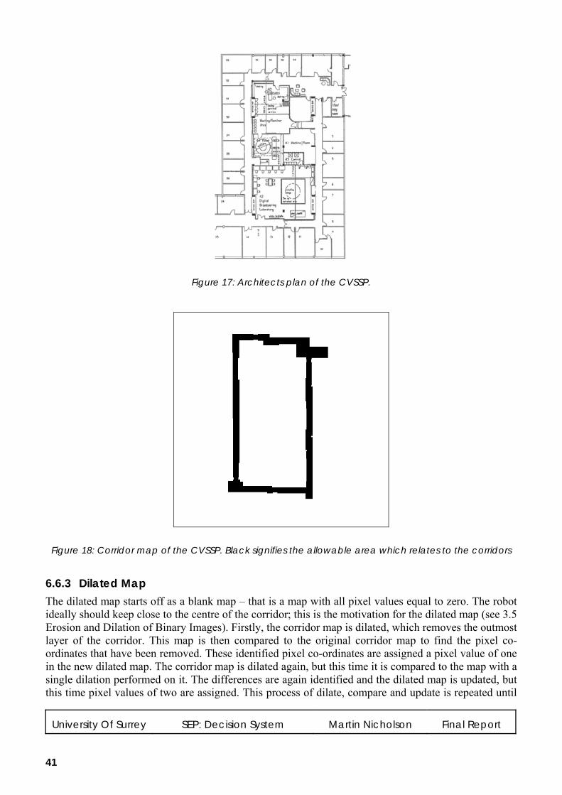
University Of Surrey SEP: Decision System Martin Nicholson Final Report
41
Figure 17: Architects plan of the CVSSP.
Figure 18: Corridor map of the CVSSP. Black signifies the allowable area which relates to the corridors
6.6.3 Dilated Map The dilated map starts off as a blank map – that is a map with all pixel values equal to zero. The robot ideally should keep close to the centre of the corridor; this is the motivation for the dilated map (see 3.5 Erosion and Dilation of Binary Images). Firstly, the corridor map is dilated, which removes the outmost layer of the corridor. This map is then compared to the original corridor map to find the pixel co-ordinates that have been removed. These identified pixel co-ordinates are assigned a pixel value of one in the new dilated map. The corridor map is dilated again, but this time it is compared to the map with a single dilation performed on it. The differences are again identified and the dilated map is updated, but this time pixel values of two are assigned. This process of dilate, compare and update is repeated until
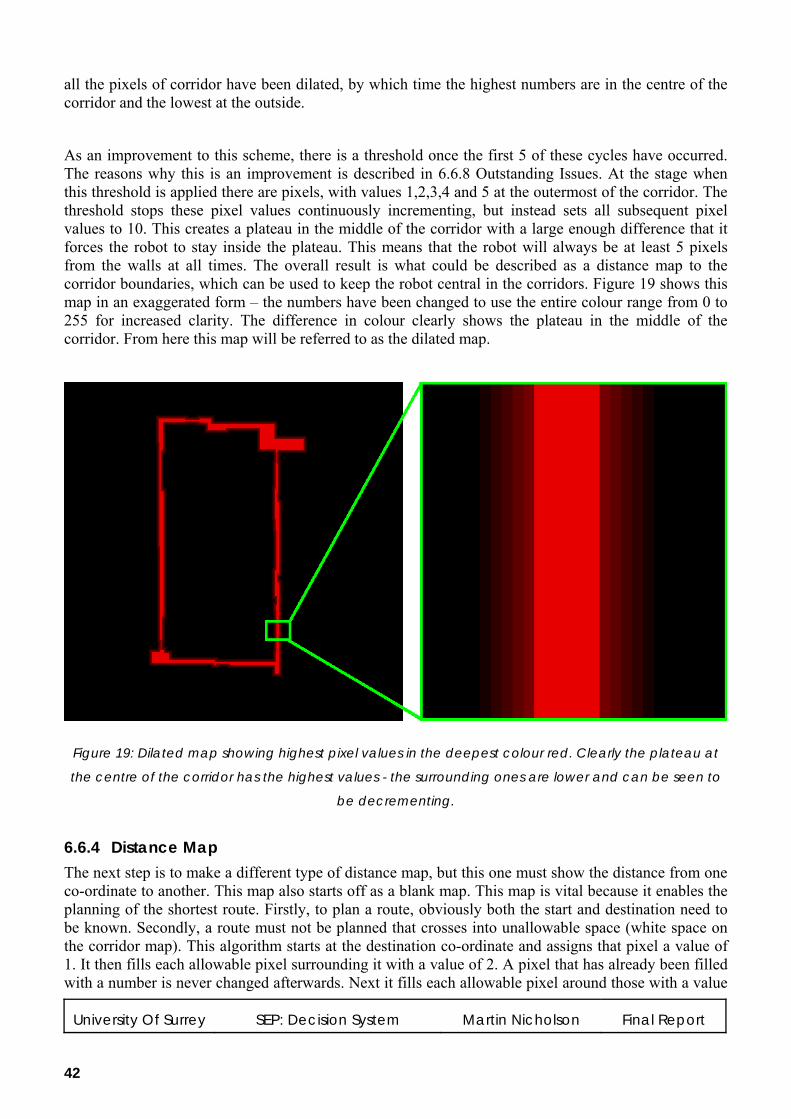
University Of Surrey SEP: Decision System Martin Nicholson Final Report
42
all the pixels of corridor have been dilated, by which time the highest numbers are in the centre of the corridor and the lowest at the outside.
As an improvement to this scheme, there is a threshold once the first 5 of these cycles have occurred. The reasons why this is an improvement is described in 6.6.8 Outstanding Issues. At the stage when this threshold is applied there are pixels, with values 1,2,3,4 and 5 at the outermost of the corridor. The threshold stops these pixel values continuously incrementing, but instead sets all subsequent pixel values to 10. This creates a plateau in the middle of the corridor with a large enough difference that it forces the robot to stay inside the plateau. This means that the robot will always be at least 5 pixels from the walls at all times. The overall result is what could be described as a distance map to the corridor boundaries, which can be used to keep the robot central in the corridors. Figure 19 shows this map in an exaggerated form – the numbers have been changed to use the entire colour range from 0 to 255 for increased clarity. The difference in colour clearly shows the plateau in the middle of the corridor. From here this map will be referred to as the dilated map.
Figure 19: Dilated map showing highest pixel values in the deepest colour red. Clearly the plateau at
the centre of the corridor has the highest values - the surrounding ones are lower and can be seen to
be decrementing.
6.6.4 Distance Map The next step is to make a different type of distance map, but this one must show the distance from one co-ordinate to another. This map also starts off as a blank map. This map is vital because it enables the planning of the shortest route. Firstly, to plan a route, obviously both the start and destination need to be known. Secondly, a route must not be planned that crosses into unallowable space (white space on the corridor map). This algorithm starts at the destination co-ordinate and assigns that pixel a value of 1. It then fills each allowable pixel surrounding it with a value of 2. A pixel that has already been filled with a number is never changed afterwards. Next it fills each allowable pixel around those with a value

University Of Surrey SEP: Decision System Martin Nicholson Final Report
43
of 2, with a value of 3. This concept is illustrated in Figure 20. This continues throughout the entire map until every allowable pixel has now been replaced with a distance (in pixels) away from the original point. From this map it is possible to find the distance, in pixels, from the destination by simply retrieving any allowable pixel value. Figure 21 shows this map in an under exaggerated form – the numbers have been reduced to only range from 0 to 255 for increased clarity. This map will be referred to from here as the distance map.
Figure 20: Illustration of the distance map at a T-junction. Each number represents a pixel, and the
value of that number is the value of that pixel. The destination is given a pixel value of 1. All the other
are the distance in pixels from that point.
Figure 21: Distance map showing increasing distance from a point in the top left corner

University Of Surrey SEP: Decision System Martin Nicholson Final Report
44
6.6.5 Path Planning Algorithm It is possible to calculate a route using just the distance map by counting down pixel values. However this route would involve travelling very close to the walls, which is not safe. Ideally the route should involve the middle of the corridor and be the shortest possible, which is conflicting because the shortest route is to cut the corners. Therefore a trade off has to be made between a safe central route and a fast route. The algorithm developed makes use of both the distance map and the dilated map to achieve this. Obviously, to plan a route requires two points – a start and a destination. Once this information is obtained then a route can be calculated.
Firstly, the dilated map needs to be calculated. Secondly, the distance map is created using the destination coordinates; hence the destination has a value of 1 and the pixel values ascend with increasing distance from this point. Each time a new route is planned the distance map has to be re-calculated, but the dilated map never needs to be changed unless changes are made to the corridor map. The algorithm starts at the starting co-ordinate. It involves taking each pixel in turn around this starting co-ordinate and finding the minimum when the pixel value in the dilated map is subtracted from the pixel value distance map. Moving to the co-ordinates of this minimum will begin the quickest route that is also safe. Then the algorithm repeats for all pixel values around that new co-ordinate. The same operation is performed on this minimum pixel, and hence its neighbour with the lowest value is moved to. This continues, until the destination point is reached.
This is made more complicated by the fact that different weights can be applied to each of the maps to change the emphasis on what the robot does. For instance a greater weight on the dilated map will force the robot to the centre of the corridor more than it will force it to take the quickest route. Conversely, a greater weight on the distance map will force the robot to take a quicker route by putting less emphasis on staying central in the corridor. It was found that using a weighting of 1:1 was not yielding the best path. By trial and error it was found that a ratio of 3:1, with the greater emphasis on the distance map, resulted in a better choice of route. This will be further discussed in 6.6.8 Outstanding Issues. An example of a planned route is shown in Figure 22.
Figure 22: Route calculated with the start location on the left and destination on the right

University Of Surrey SEP: Decision System Martin Nicholson Final Report
45
6.6.6 Refining the Map Size Initially a corridor map (Figure 18) size of 1000x1000 pixels was being used. It was just an arbitrary size. This also meant that the dilated map (Figure 19) and the distance map (Figure 21) were 1000x1000 pixels. The time taken to perform the dilation algorithm upon this map was unacceptably long. It was observed that the dilation algorithm took just below 6 times longer on the 1000x1000 map compared to a 500x500 map.
For the sake of completeness a test was performed to record the time taken by the dilation process simply by using a stopwatch. It would have been easy enough to do this test in code, but the necessity of this seemed minimal. This test was performed on varying map sizes (250x250, 500x500, 1000x1000 and 2000x2000) and the time recoded. Each map size was timed twice and the same computer was used with the same applications open to try and make it a fair test. Obviously there is error involved in starting and stopping a stopwatch, especially with the small maps when the time taken is very small. However the relationship found is clearly exponential, and a graph has been plotted to show this. The graph in Figure 23 shows the average readings taken, and a plotted exponential line of best fit. From this graph it can evidently be seen that 500x500 is a good map size because a smaller map would not save any significant time, but a larger one would take an exponentially increasing amount of time.
However, this speed increase from using a smaller map comes at the price of a decreasing resolution. The resolution of this new smaller map was calculated to check the map still had sufficiently high resolution. It is required to know the resolution for the robot to function because it must map sensor readings (in cm) onto map co-ordinates (in pixels). The corridor was measured in 4 different places. A tape measure was used to measure the real distance in each location. This was repeated 3 times in each location. The corresponding regions on the map were then identified and their width in pixels was then counted. The distance was divided by the number of pixels to give the cm/pixel value; these results can be found in Figure 24. This table shows that, as expected, each pixel represented less as the map got bigger – indicating a higher resolution. The errors also decrease as the map gets bigger. On the 500x500 map each pixel was calculated to be approximately 10x10cm. This resolution is acceptable and the robot is unlikely to ever need better.
The results shown in Figure 24 were plotted onto a graph as shown in Figure 25. This graph has a line of best fit showing that resolution starts to stabilise at around a map size of 1000x1000 pixels. It also shows that with a map size of less than 400x400 the resolution starts to drop rapidly (note that a high cm/pixel relates to a low resolution). Hence choosing a size of 500x500 is a good choice.
As a result the map size was permanently changed to 500x500 pixels because it represented a good choice for both the speed of image processing and a good choice for the resolution.

University Of Surrey SEP: Decision System Martin Nicholson Final Report
46
Average Time Taken To Dilate Different Sized Maps
0
50
100
150
200
250
300
350
0 500 1000 1500 2000 2500
Map Size (Pixels)
Tim
e (S
econ
ds)
Figure 23: This graph shows the average time taken to dilate different sized maps. The values are
plotted as well as an exponential line of best fit.
Map size (pixels) Distance Represented By Each Pixel (cm/pixel)
Location 1 Location 2 Location 3 Location 4 Average σ
250 19.00 18.00 20.29 18.19 18.87 0.90
500 10.23 9.60 10.14 9.09 9.77 0.46
1000 4.93 4.80 4.90 4.55 4.79 0.15
Figure 24: Table showing the calculated resolution at different map sizes.

University Of Surrey SEP: Decision System Martin Nicholson Final Report
47
Resolution Of Different Sized Maps
0.00
5.00
10.00
15.00
20.00
25.00
0 200 400 600 800 1000 1200
Map Size (pixels)
Dist
ance
Rep
rese
nted
By
Eac
h P
ixel
(c
m/p
ixel
)
Figure 25: This graph shows the average resolution in cm/pixel for different sized maps. The values are
plotted with error bars and there is a line of best fit.
6.6.7 Improvements Made The map size reduction improved the speed dramatically. The speed was also improved by using compiler optimisations in Linux and using ‘release’ mode in Windows.
Occasionally there was an issue where this route planning algorithm would alternate between two pixels (i.e. once it moved to the next pixel the minimum was to go back again and this continues indefinitely). The reason for this was identified to be the fact that some parts of the corridors are wider than others. This meant that when the corridor map was dilated the values in the narrow parts of the corridors were higher than those in the wide parts. To fix this, a high number is assigned to each pixel visited so that it will not be chosen again. Figure 22 shows a line representing the quickest route. In reality the same line is drawn using this technique but in a different pixel value and hence a different colour.
The path planning concept has been extended so that a default start location is used and by simply clicking the map displayed on screen with the left mouse button will set the destination. It will calculate the route to that point, if that point is valid. This point then becomes the robot’s new start location and clicking again will set a new destination. This makes is quicker and easier to check the accuracy of the path planning. It will also enable testing when integrated with the external image processing system, which must send coordinates.
6.6.8 Outstanding Issues There are two issues still unsolved with the path planning algorithm developed. These issues were seen as minor and due to limited time they have been ignored so that progress could be made on other sections. They have no negative effect on planning a path using the 500x500 map. However, they decrease the portability of the system because some parameters have had to be fine tuned for each particular map.

University Of Surrey SEP: Decision System Martin Nicholson Final Report
48
The plateau created when the dilation algorithm is performed on the corridor map is one of these issues. The plateau is explained in 6.6.3 Dilated Map. The dilation algorithm is not perfect because the corridors are not simply parallel lines with an equal width. There are irregularities such as stairs, doors and two large open areas. Hence when the dilation algorithm is run the centre of the corridor is not assigned the same value everywhere on the map. This is illustrated in an exaggerated example shown in Figure 26. It shows a thin section of corridor attached to a think section and clearly the thin part of the corridor has a maximum value of 2 whereas the thick part has a maximum value of 5. The green signifies where the robot started and the purple shows its destination. Using the algorithm described, the robot will take a very inefficient route illustrated by the red path. The dilated map is subtracted from the distance map and so high numbers are travelled through in preference to low numbers. Therefore, when the robot approaches the blue line, the minimum pixel when both maps are combined is not straight ahead. The minimum is to go round in circles until all the pixels with a value higher than 2 have been travelled through and hence given a high value. Then, and only then, the robot will continue straight ahead into the thin corridor. Thus the cause is because of the relatively sudden drop in pixel values when entering the thin section of the corridor.
In reality the corridors are much wider than the illustration. They all are many more than 10 pixels wide (representing about one meter in reality), therefore setting the threshold to 5 means that in every instance the threshold is met. The plateau ensures that the centre of the corridor is uniform value of 10 everywhere. Thus, the problem was resolved. However when a different map is used, such as the 1000x1000 map, the threshold needs modifying for optimal path planning. In the case of the 1000x1000 map, the threshold can simply be doubled; likewise the plateau value also needs doubling. If these two parameters were closely related to the map size a section of code could be added to compensate. The real problem occurs when a completely different map is used. Therefore this is not the perfect design.
The other issue is when the dilated map is subtracted from the distance map there is a weighting ratio of 3:1, with the greater emphasis on the distance map. This was discussed in 6.6.5 Path Planning Algorithm. The basis for this ratio was determined by trial and error. The theory behind it is that the pixel values to the destination on the distance map only decrease by 1 each time and due to corners the robot does not always follow the ideal path. Consider Figure 27 for an example on a T-junction, which is where the effect is worst. As the robot travels from the top of the illustration to the destination at the bottom it is also trying to stay central in the corridors due to the dilated map. However, the dilated map has a plateau in the middle so there is no advantage of being exactly central in the corridors. Therefore it tries to cut the corner slightly and ends up swerving into the corridor to the left. It then comes back on itself to reach the destination. Setting a higher weighting for the distance map compared to the dilated map smoothes this issue substantially because the robot comes back on itself sooner than it otherwise would. This weighting may need changing if the map were significantly different.
If this were a production system, then perhaps a configuration file could be read at start-up, along with the map. This configuration file would make fine tuning these parameters and weights easier. As an extension to this, a simple calibration program could be written that plans many paths using various parameter values and weights on the given map, and asks the user to choose which route is best. It then could save the optimal parameters and weights to a configuration file to be read on start-up by the main program.

University Of Surrey SEP: Decision System Martin Nicholson Final Report
49
Figure 26: Exaggerated illustration of the issue faced when dilating a map. The blue line shows the
sudden change in numbers caused by a thin section of corridor attached to a think section. In reality
the blue line would be closer to a semicircle shape and lower. However, it clearly shows the issue
faced because the thin part of the corridor has a maximum value of 2 whereas the thick part has a
maximum value of 5. The green signifies where the robot started and the purple shows its destination.
The red illustrates the route the robot might take.
Figure 27: Illustration of the route the robot might take at a T-junction. The pixels visited are represented
by the red boxes around the pixel values. It starts at the top with a pixel value of 9. It swerves slightly
into the corridor to the left but eventually reaches the destination (signified by a pixel value of 1).

University Of Surrey SEP: Decision System Martin Nicholson Final Report
50
6.6.9 Conclusions The path planning algorithm is now very reliable and plans a close to optimal path each time. In some regions of the map the optimality of the calculated route is better than others. But even in the worst case scenario the route is close to the optimal one than a human could draw. There are some minor outstanding issues but these are considered insignificant because for the intended purpose it works.
6.7 Location Estimation
6.7.1 Introduction The decision system can successfully plan routes from a given starting location (the current location of the robot) to a given destination. However, the current location will never be exactly known and given in a straightforward fashion. The next step was to try and identify the robot’s current location from noisy estimates. This task is more difficult. The external image processing system will send estimates of the robot’s location, the accuracy of which depends upon how close the robot is to a camera. It will also send a destination to the robot where there is human activity. The wireless positioning system will also send estimates of the current location, although the variance is likely to be larger. From these inputs the decision system must obtain a reasonable estimate of the current location along with an overall uncertainty.
6.7.2 Implementing a Kalman Filter A Kalman filter was selected to accomplish this task. The reason for which was because of the success of numerous other projects also using a Kalman Filter (some examples are given in section 3.4.2). They are commonly used in robotics and seemed like a sensible choice. Before this project, the author had no knowledge or concept of Kalman Filters, or even a covariance matrix! Much research and understanding was the first thing required. The first approach taken was based on some Kalman Filter formulas. It was quickly realised that for the intended purposes this could become complicated. Therefore existing packages were used (see 3.9 Filtering Libraries Available for C++). Firstly, Bayes++ was tried, which although initially looked very promising, was unsuccessful and a large waste of time. Then the use of an equivalent library called the Bayesian Filtering Library was explored. In the end the more basic Kalman Filter inside OpenCV was chosen.
6.7.2.1 Using Formulas The first attempt involved manually writing basic Kalman filter formulas in the code.39 The route planner program was adapted so that a click with the right mouse button on the displayed map would be treated differently from the left mouse button. This would represent an estimate of the robot’s location given by the external image processing system with a default uncertainty used for simplicity. The location of the robot was influenced by this input; the extent of which depending upon the uncertainty used and the location given. The original plan was for it to be possible to specify an uncertainty with each right click of the mouse. This however, became cumbersome, and was dropped from the design. The final state of the system successfully drew the correct sized circles on the map. It could adjust the estimate of the current location based upon new estimates given with the right mouse button. A click of the left mouse button would then plan a path from the estimated location to the specified location.
39 Maybeck, P. S., Stochastic Models, Estimation, and Control, Volume 1, Academic Press Inc., 1979, chapter 1

University Of Surrey SEP: Decision System Martin Nicholson Final Report
51
Although this seemed initially successful there were a number of obvious issues. The formulas used only took variances into account and not covariance matrices. Hence if all the readings only varied in the x-axis the overall uncertainty was still needlessly a circle. There were no dynamics in the model used. It soon became obvious that the amount of work required to properly implement the Kalman filter using the basic formulas was high. Much matrix manipulation would be required, which may have required the use of an extra library. Therefore the decision to try an existing package was taken.
6.7.2.2 Using Bayes++ Bayes++ initially looked very promising and contained a large choice of filters. Its developer was involved with the Australian Centre for Field Robotics.26
The first task was to download and install the Boost Library25. Once this was accomplished the source code was also downloaded and unpacked. There were a number of examples included and a ‘solution’ for use with Microsoft Visual Studio. This solution was created in an older version of Visual Studio and required converting by Visual Studio 2005. The compiler paths were changed so that the compiler could locate the Boost header files. This should have been adequate to have built the examples. However, there was a compilation and the examples would not compile. Much research on this problem was carried out to try and solve it. It was discovered that the issue was being caused by the Boost libraries and not by Bayes++.
Further research continued and eventually an internet forum thread was found where someone else had identified the same problem.40 The response to this message included a workaround for the errors. The author of the response claimed that the problem was with Visual Studio 2005 giving bogus warnings and errors. The author also stated he had only just obtained the new version of Visual Studio. This suggests that maybe most people using the Boost libraries with Visual Studio may still be using older versions of Visual Studio and hence have not noticed this issue.
The workaround enabled the examples to compile. These examples were then examined in order to understand the syntax. It was attempted to merge the simplest example into the route planning code to check compatibility. The ‘solution’ for Bayes++ must have had many settings changed in order for it to compile because there were hundreds of errors given. Instead of wasting more time copying settings it was attempted to merge the route planning code into the simplest example. There were far less errors produced as a result. Once the Network API was removed the compilation worked. Much time was spent trying to understand Bayes++. It was discovered that some operations had been given different names than the convention. For example the term ‘observe’ was used instead of the conventional ‘update’. These, although minor changes, caused unnecessary confusion. Eventually, after a distinct lack of progress, the decision was made to give up with Bayes++ and move onto a different library.
6.7.2.3 The BFL (Bayesian Filtering Library) A message was found in the Bayes++ message forum stating about the lack of documentation and the 40 Stevens, M., Re: Compilation problems from a ublas newbie, http://article.gmane.org/gmane.comp.lib.boost.ublas/2473,
2006

University Of Surrey SEP: Decision System Martin Nicholson Final Report
52
tedious installation procedure. It suggested many people were put off using it, and instead were using the BFL.41 This prompted a brief exploration of the BFL. However, time was scarce and although the BFL was considerably better documented than Bayes++, it was thought that it was still a complicated library and something more basic should be chosen.
6.7.2.4 OpenCV Therefore the relatively simple Kalman Filter inside OpenCV was chosen. The package was downloaded and installed and the relevant compiler paths were given. The OpenCV library files were linked to the decision system ‘solution’. The example contained within the OpenCV package was overly complicated because it contained a full GUI. Therefore a simpler example was searched for and easily found on the OpenCV message forums42. This was used to understand the syntax and general concepts. It soon became clear on how one might implement a Kalman Filter for a similar purpose using just one input. The biggest issue arose from the need to specify multiple inputs at each time step. The Kalman Filter inside OpenCV was relatively basic and therefore there was no way to state the time step when specifying an update. It assumed every update took place at a new time step and expected a constant ‘predict-update-predict’ cycle. This seemed to be what users of the OpenCV Kalman filter wanted to do because there is no information about performing multiple updates in each cycle. A way to stop the dynamics would have been a good workaround, but no way of achieving this was found either.
The solution came from trial and error. It was possible to input a measurement into the Kalman Filter and then manually copy the prior state information into the post state information. This was an ad-hoc solution but seemed to work. This allowed different covariance matrices for each input. Using this technique it was possible to input multiple updates without continuing with the dynamics. This concept was used in the decision system to merge the wireless positioning system input with the external image processing system input.
6.7.3 Emulation Programs In order to test the devised Kalman Filter it was necessary to have the means of inputting coordinates manually for each cycle. This meant it was possible to give both accurate and inaccurate readings and check the response of the Kalman Filter. The fact that the Network API is present in most of the decision system code allows other programs to connect to the decision system and send coordinates. It was first envisioned that the program used to connect to the decision system would be an existing Terminal application. However, entering coordinates by typing them was never a good solution because it would be slow and cumbersome. Therefore, some emulation programs were created to imitate the systems that the decision system would be communicating with. This not only can be used to test the Kalman Filter, but also can be used to identify problems that may occur during an integration attempt. They are intended so that the decision system could not tell the difference between the real application and the emulation program. Therefore the emulation program must use the same parameters and send the data in the same order.
41 Bellotto, N., Bayes++ docs and installation,
http://sourceforge.net/mailarchive/message.php?msg_id=200603121923.46344.nbello%40essex.ac.uk, 2006 42 http://tech.groups.yahoo.com/group/OpenCV/, Message ID 28687
University Of Surrey SEP: Decision System Martin Nicholson Final Report
53
6.7.3.1 External Image Processing System The external image processing emulation program has two modes. The first mode shows the map on screen in a GUI and two clicks are required to set the current location estimate and the destination. The variance in x and y are preset for the sake of speed and simplicity. This method can take a long period to send the robot down a corridor so there is a second mode that is completely automatic. The readings are incremented and sent in such a way that the location estimation program believes the robot is moving down the corridor. This emulation program can also be used with the route planner program to define a route to plan.
6.7.3.2 Wireless Positioning System The wireless positioning emulation program also has two modes. The first mode shows the map on screen in a GUI and a single click is required to set the current location estimate. The variance in x and y are also preset for the sake of speed and simplicity. Again, there is a second mode that is completely automatic. The readings are incremented and sent in such a way that the location estimation program believes the robot is moving down the same corridor. This emulation program is slightly more complicated because the real wireless positioning system must receive a command to start taking measurements and send coordinates back in a requested number of seconds.
6.7.4 Testing The testing of the location estimation was done using the described emulation programs. It was carried out by changing the inputs and observing the estimated location. A more formal testing method could not be really be used for the nature of this scenario. In many of the tests there were massive numbers of coordinates used and to write all these down would take many pages and probably be meaningless to the majority of readers. Instead, each test has been briefly described and a reason has been given why it passed that test. Numerous screenshots have also been avoided, with just one to give the reader an idea of what is happening in the test. This is shown in Figure 28. In most of the tests the automatic mode was used in the emulation programs to save time. The coordinates sent were varied by re-compiling the emulation programs for each test.
6.7.4.1 Ideal Situation The emulation programs in this test passed almost ideal coordinates. This is because both the emulation programs send roughly corresponding estimates that are fairly close to each other and move in the same fashion. As one would expect the estimate produced by the Kalman filter is a location between the two estimates with a greater emphasis on the measurement with lower variance. The output is shown in Figure 28.
6.7.4.2 Constant Situation When the emulation programs send the same constant coordinates many times the location estimated is, as one would expect, that static location. Note that initially the Kalman filter applies some preset dynamics which despite no movement from the inputs still cause the initial few estimates to move slightly away from this static area. After about three or four readings the estimate moves back to where it should be.

University Of Surrey SEP: Decision System Martin Nicholson Final Report
54
6.7.4.3 Conflicting Information This is a more real world situation because there is likely to be inconsistency in the different estimates. For this test the wireless positioning emulation program gave a constant estimate each time. The external image processing emulation gave an estimate that constantly moved down the corridor. This could happen in reality if there was an error with one of the systems. The location estimated followed the movement of the external image processing system but at a slower rate. At one stage each input was at a different end of the corridor and the estimate produced was somewhere around the centre of the same corridor.
6.7.4.4 Similar Movement followed by being stationary In this situation both emulation programs input estimates that move down the corridor and then both sent stationary ones at slightly different locations. This performed as expected with the estimate stopping near between the two emulation programs estimates. However, the author had expected to see some overshoot when the readings became stationary to reflect the sudden change in dynamics.
6.7.4.5 Individual Clicking The final test involved using the emulation programs in their other mode, which is where one clicks the map each time to send as estimate. This takes longer but has the advantage of far greater control. Various different inputs were sent from both emulation programs. Sometimes these estimates correlated with each other and sometimes a random extremely noisy one was sent. In each case the outcome was observed. Each observed estimate always lay roughly where the author expected them to. Obviously, knowing exactly where the estimate should lie is impossible, but in the author’s opinion they were good estimates.
6.7.5 Conclusions The process of implementing the Kalman filter was more complicated than expected. The slightly unusual design requirements, like needing multiple updates in each step, could have contributed to this. The implemented Kalman filter produces good estimates and as such has been counted a success.

University Of Surrey SEP: Decision System Martin Nicholson Final Report
55
Figure 28: Screenshot showing a typical test. In this test both emulation programs are sending
coordinates down the corridor, each slightly different. As expected the location estimated is very
similar to these estimates. The blue arrow represents the current estimation of the robot’s location. The
ellipses represent the uncertainty. In this case the outermost one represents the wireless positioning
system estimate and the innermost one represents the external image processing estimate. The middle
one represents the uncertainty of the Kalman filter.
6.8 Sensor Fusion
6.8.1 Introduction The sensor readings provided by the drive management system were unprocessed. They merely had been converted into centimetres.32 Therefore it was the task of the decision system to make them into something useful. They obviously could be used at a low level to check that a collision is not about to occur before issuing movement commands. But they could also be used for more than this. For example, using these sensors the decision system would know exactly how far it is away from the two side walls of the corridor. Theoretically the ultrasound sensor readings are the most accurate information provided. They only contain distance information and do not contain any direct mapping to particular coordinates. The aim of the sensor fusion part of the decision system is to provide an additional input to the Kalman filter by attempting to map the distance readings into coordinates.

University Of Surrey SEP: Decision System Martin Nicholson Final Report
56
It was envisioned that the expected sensor readings could be compared to the actual sensor readings to help estimate the robot’s location. It was thought that the difference between each sensor’s expected reading and real reading could be used to determine if either a translation or a rotation was required. If either were required then it would be possible to simply update the current estimated location with this. This new estimate could then be used as another input in the Kalman filter to further help determine a new estimate of the current location.
This section begins by outlining the program used to obtain estimated sensor readings. It then leads onto a brief section discussing the real sensor data.
6.8.2 Expected Sensor Readings Real sensor data was not available until close to the end. Therefore a good starting place was to calculate the sensor readings that might be expected at a given location. This is possible by taking each sensor in turn and projecting a line out until it reaches the unallowable part of the map. The point of each intersection is stored along with the current location. From this, the distance can be determined in pixels. This algorithm developed can have any angle of rotation specified and still work. The sensor angles are hard coded at 45° intervals between 0° and 360°. If a sensor does not reach an unallowable part of the map after 40 pixels (≈4 metres) it is stopped and given a value of 40 pixels. Figure 29 shows the program used to find the expected sensor values. The lines drawn can be seen on the map as well as the output of the different readings in the terminal.
The problem determined with the expected sensor results was that sensor readings could relate to almost anywhere on the map. Some random locations were used to obtain sensor estimates and many were close to being identical. This problem is illustrated in Figure 29 where two completely different locations have virtually identical distance expectations.
It could however be used to determine rotation, if the current location was known. Figure 30 shows a promising result of two sensor estimates in the same location, but with a 10° orientation difference. The values are significantly different and therefore it may be possible to correct the orientation of the robot by comparing the real sensor readings with the expected ones. This does depend however, upon how close these expected sensor values are to the real sensor values.
6.8.3 Processing Real Sensor Data As mentioned earlier the real sensor data was not available until the end of the project. Hence time to process the sensor data was limited. The data was obtained as described in section 7.2.3. Sensor data was quoted as being accurate to within approximately 1cm.32 However, once some real sensor data was captured, and the limited remaining time was used to process the readings it was discovered that this may not be the case. The problem is shown in Figure 31 which shows 4 randomly taken samples. The sensor readings seem to bear no correlation to the corridor shape. This is a massive setback to the sensor fusion ideas.
6.8.4 Conclusions The initial sensor readings obtained were not promising. However, there was not enough time to fully
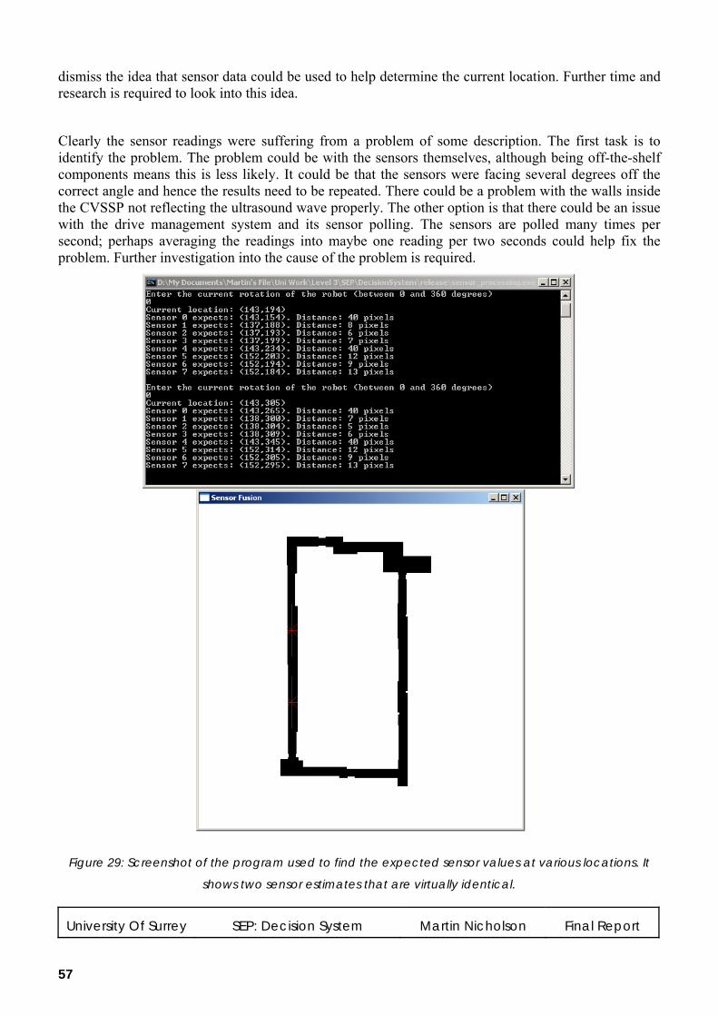
University Of Surrey SEP: Decision System Martin Nicholson Final Report
57
dismiss the idea that sensor data could be used to help determine the current location. Further time and research is required to look into this idea.
Clearly the sensor readings were suffering from a problem of some description. The first task is to identify the problem. The problem could be with the sensors themselves, although being off-the-shelf components means this is less likely. It could be that the sensors were facing several degrees off the correct angle and hence the results need to be repeated. There could be a problem with the walls inside the CVSSP not reflecting the ultrasound wave properly. The other option is that there could be an issue with the drive management system and its sensor polling. The sensors are polled many times per second; perhaps averaging the readings into maybe one reading per two seconds could help fix the problem. Further investigation into the cause of the problem is required.
Figure 29: Screenshot of the program used to find the expected sensor values at various locations. It
shows two sensor estimates that are virtually identical.

University Of Surrey SEP: Decision System Martin Nicholson Final Report
58
Figure 30: Two sensor estimates obtained at a 10° orientation difference. There is a significant
difference in the distances expected.
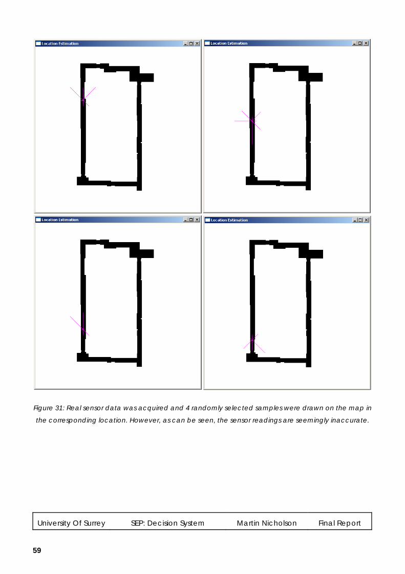
University Of Surrey SEP: Decision System Martin Nicholson Final Report
59
Figure 31: Real sensor data was acquired and 4 randomly selected samples were drawn on the map in
the corresponding location. However, as can be seen, the sensor readings are seemingly inaccurate.

University Of Surrey SEP: Decision System Martin Nicholson Final Report
60
6.9 Movement Commands The current state of the decision system has not implemented any movement commands. However, this is a trivial task. It is also the last task to be implemented because until the sensor data can be processed fully then robot orientation cannot be found and hence drive command executed accurately.
It is planned to move the robot for a short distance, maybe a metre or two, and then stay stationary for about 5 seconds while the wireless positioning system estimates the current location. Meanwhile the external image processing system should have been sending repetitive coordinates which will reduce the overall uncertainty of the current location estimate. Then the sensor readings can be averaged and used to further help with the estimation. Movement could commence again when all this has occurred. Each time before movement is made the sensor readings need to be checked in order to determine whether it is safe to move. While the robot is moving it needs to continuously check the sensors in order to avoid any collisions. This process must repeat until the destination specified is reached.
6.10 Decision System Internal Integration The decision system has been presented throughout the report as many individual sections and programs. In reality the decision system code has all been integrated. This method allows for greater flexibility because aspects are designed separately and when complete, they are merged with the rest of the code. As detailed in section 7.2.2, the aim of Easter holiday integration attempt was to display information on the decision system map. This information includes the expected sensor readings, the route planned, the current location and destination, and the confidence ellipses. This integration attempt was a failure for the group, but not for the decision system. As shown in Figure 32, the decision system was able to show all the required items neatly on screen. This screenshot was achieved by using the emulation programs. As previously mentioned, by using the emulation programs the likelihood that the decision system would have a problem at an integration attempt is decreased.

University Of Surrey SEP: Decision System Martin Nicholson Final Report
61
Figure 32: The decision system showing the expected sensor readings in purple, a planned route in red,
the destination as a box and the start as an arrow. The confidence ellipses represent the uncertainty of
the external image processing system (purple), the wireless positioning system (brown) and the current
estimate (green).

University Of Surrey SEP: Decision System Martin Nicholson Final Report
62
7. Integration Effort
In this section some of the key integration attempts are discussed. A diary style approach has been avoided as much as possible, but as each attempt builds upon the last there is a requirement for it to be presented in chronological order. As such it has been broken into two sections – one for each semester.
7.1 Autumn Semester Near the end of the autumn semester the team were at a stage to try and integrate various components of the robot. The first stage was to fix the frame onto the chassis, then fix the laptop onto that. The camera was temporarily taped onto the frame so that video footage could be taken and processed at a later date by Peter Helland. The laptop was connected to the motor controller and the motor power was obtained from a power supply (the batteries had not arrived by that stage). The robot was sent a few metres forwards and stopped by cutting the power supply. To make the video footage more useful varying speeds were captured and in some of them people were moving in view of the camera. Figure 33 shows the temporary setup used. The video footage obtained was useful to Peter Helland and it was helpful for determining the speed the robot was travelling at. This integration attempt was successful because the robot moved in the correct direction and it proved that the laptop’s USB 2.0 expansion ports worked for the webcam. This mainly integrated work by Edward Cornish and Peter Helland.
The next integration phase involved using the network API to communicate between the decision system and the external image processing system. This proved more complicated and was only partially successful. The decision system integrated with the Network API and would receive coordinates if a program like HyperTerminal was used to send them. However there was a problem with the external image processing system which was causing the code not to compile. It was found the fault was not with the Network API, but instead with the external image processing system. The code would not compile if certain standard libraries and function calls were used. This integration attempt was partially successful. It was invaluable because it determined problems early and hence they could be fixed by the spring semester. This phase integrated work by the author, Peter Helland and Ahmed Aichi.
Figure 33: Photograph of the temporary setup used for the first integration attempt

University Of Surrey SEP: Decision System Martin Nicholson Final Report
63
7.2 Spring Semester The spring semester was when the majority of the integration occurred. The problem with the external image processing system was resolved and hence it could be integrated with the Network API. This section details some of the key accomplishments achieved by the team.
7.2.1 Decision System and External Image Processing System Communication Due to the fact that the Network API could be integrated with the external image processing system, communication was again attempted between the two systems. The aim was for the external image processing system to send two sets of co-ordinates to the decision system. One was the current location estimate and the other was the destination. There were initial problems such as the old 1000x1000 map was still in use by the external image processing system. However, by the end of the integration attempt communication was successful. The coordinates sent were identical each time but this was irrelevant because a path could still be planned between both points. This attempt was therefore a success because the aims had been met. This integrated work by the author, Peter Helland and Ahmed Aichi.
7.2.2 Easter Holiday Integration Attempt The original aims were set before the Easter holiday. The aim was to remote control the robot around the corridors while receiving estimates of its location from the wireless positioning system and the external image processing system. From these estimates the decision system could estimate a location and display it on the map. This required input from all the team members. Despite spending a long day, the integration was unsuccessful.
This was partly because the wireless positioning system could not be used during the day time for fears of service interruption for other users. It was partly because the external image processing system was not ready. None of the aims were met so this integration attempt was considered a failure.
7.2.3 Sensor Measurements Edward Cornish had managed to get the sensors working in time for the integration attempt just after the Easter holidays.32 This meant some sensor readings were taken that could be processed later. In order for the sensor readings to be meaningful the external image processing system also provided estimates of the location so that each sensor reading could be mapped. Both systems created output files, with each entry containing the data and a timestamp. The clocks of the computers involved were synchronised using a world time server. This meant that the two files could be processed together to show a location on the map and the corresponding sensor readings. The processing of this sensor data is discussed in section 6.8.3. This integration attempt was therefore successful because results were obtained.

University Of Surrey SEP: Decision System Martin Nicholson Final Report
64
8. Conclusions
During the course of this project much progress has been made on the decision system. A universal map of the patrol area has been made and a route can be planned from any one coordinate to another. This route is safe, in the way that it tries to keep the robot in the centre of the corridors hence reducing the chances of a collision. This route is also short. Each time a route is calculated it close to the most optimal route that could be possibly be calculated. This part of the decision system has been a success.
The decision system has been successfully integrated with the Network API.31 This has not only allowed various integration attempts to take place, but it has also enabled several separate emulation programs to be written. These emulation programs were invaluable in testing the location estimation part of the decision system.
The location estimation part has been the longest delayed part of the project. Its purpose was to estimate the current location of the robot from multiple noisy observations. To accomplish this, a Kalman filter was used. There have been numerous problems in implementing such a Kalman filter. The main causes of the delays were due to two implementations that were fundamentally flawed (see sections 6.7.2.1 and 6.7.2.2). Obviously this was not known beforehand, but each implementation wasted valuable time. Eventually OpenCV was used for its Kalman filter. Although it was relatively basic compared to other libraries available, it suited the role perfectly. In an ad hoc way it was possible to specify multiple updates at each time step. This was tested using the emulation programs and it produced sensible location estimates based upon the given input.
High hopes lay on the sensor fusion ideas. It is possible to theoretically predict the sensor readings at a known location and a program has been written that will accomplish this. However, judging by the initial results, they may have no correlation to the real measurements. The initial results were disappointing, but further investigation is required to find our why they were so inaccurate. Currently, there is no orientation hardware fitted to the robot and as such this sensor data is all that can provide rotational information. Theoretically the sensor data is sufficient if a known start orientation is provided, because the robot can sense and correct any minor rotational errors. A problem would occur if a cumulative rotational error of over 45° were to occur however. Ideally the robot would have featured a compass and this is definitely a possible future improvement.
Creating movement commands is a trivial aspect of the design of the decision system. The interfacing to the drive management system was decided upon in the autumn semester. However, time was limited and this was not implemented.
Currently the decision system is not totally finished. The severe difficulties encountered with the Kalman filter were the main cause. However, the author still believes that this project was a success because the majority of the work has been carried out successfully. The work carried out has successfully been integrated with the various other systems, which is a crucial aspect to the working of the robot.

University Of Surrey SEP: Decision System Martin Nicholson Final Report
65
9. Discussion
It is a great shame that time was marginally too short to create a fully working robot. It would have been an impressive showcase for visitors to the university and potential future students. Maybe if the project is continued in the future then it can become a fully finished invention.
If I could change one thing about how I undertook the project, it would be to have known when to give up on Bayes++. This probably should have been after about 2 weeks. The lack of documentation and the errors encountered should have put me off using it sooner. If I had used the OpenCV Kalman filter from the start I think I would have finished the project on time. There was never going to be a large amount of time to spare, so even if I had used OpenCV from the start, the deadlines would have still been challenging to meet, but they would have been obtainable.
The delays in other team member’s parts of project also caused some hindrances; such as having to wait until week 11 for real sensor data and corresponding external image processing location estimates. However, this is not to blame for the project not being finished on time because emulation programs could have been used to produce purely theoretical results.
It is a shame that I was not able to use a major robotics library, such as the BFL or Bayes++, because it was something that not only could have benefited the project, but also would be good for my own personal experience.
I have found this project extremely useful and have learnt loads from it. I have not only learnt vast amounts of technical knowledge but have also picked up invaluable life skills. I personally think that level 3 group projects are an excellent idea because they prepare us for the real world in a way that no individual project could. They do however have an associated overhead, but as a group the outcome will be more than that of a single person. Although I think that this project has been a large amount of work compared to a typical level 3 project, I am thankful that I was apart of it. I hope that Dr. Bowden will continue this project in the future and that the department as a whole will consider group projects as a more feasible option.

University Of Surrey SEP: Decision System Martin Nicholson Final Report
66
10. Future Improvements and Developments
The path planning using the current map is close to perfect. However, there are some parameters that may have to be fine tuned if the map were changed.
The real sensor readings obtained need further time to determine if they are useful or not. The random samples chosen may have been unrepresentative. Otherwise, the problem needs to be identified and perhaps then the sensor data can be used to help estimate the robot’s current location and rotation.
The movement commands need adding to the path planning algorithm. This is a trivial task because the robot can already estimate its current location and it can already plan a path to its destination.
Other possible improvements include the refinement of the corridor map using the sensor readings as the robot travels around the corridors. The original corridor map will still be required however, to enable the universal coordinate system. This will be achieved by using a probability range for each pixel instead of just black or white. As the robot travels it will have a rough idea of its location at any given time and will use the ultrasound sensor readings to update the map. By using a 256 colour image it is possible to start with the corridor map, but change each pixel to use 0 for black and 255 for white. Then, as the robot travels, it can increment or decrement those values depending upon the sensor readings. For example if someone were to put an object the size of one pixel in the middle of the corridor, that pixel would originally be 0, and with each pass it would be incremented. As it gets higher the path planning algorithms will ignore it and eventually it will reach 255 and be officially out of bounds. If the object was then removed, the opposite would happen, with it eventually reaching 0, hence being the same as the original value.
Another additional feature that should be added is a pedometer of some sort. This could be a system using optic encoders. The original plan included a pedometer so that the decision system knew exactly how far the robot had travelled. This would give a better idea of how far the robot moved, compared to relying upon how far the motors were supposed to move it. This is because the distance moved by the motors will depend upon the incline, the state of the battery and the previous speed. A pedometer could vastly improve the accuracy of the robot’s estimated location.
Finally, the robot needs some form of hardware to identify its orientation. An electronic compass was investigated by Edward Cornish but never actually implemented due to a lack of time.32

University Of Surrey SEP: Decision System Martin Nicholson Final Report
67
References
[1] RoboCup@Home, http://www.robocupathome.org/, 2007
[4] Kittler, J., Machine Intelligence Handout, University Of Surrey, 2007, pages 2-3
[5] UNCE, IFR, 2005 World Robotics Survey, Press release ECE/STAT/05/P03, 2005
[6] Fowler, J., U.N. sees coming surge in domestic robots, Associated Press, 2004, http://www.usatoday.com/tech/news/robotics/2004-10-20-robot-report_x.htm
[7] RI-MAN revisited, 2006, http://www.pinktentacle.com/2006/03/ri-man-revisited/
[8] Robot special: Almost human, New Scientist Magazine, Issue 2537, 2006, page 38, http://www.newscientist.com/article.ns?id=mg18925371.800&print=true
[9] Boyd, R. S., Machines are Catching Up with Human Intelligence, Knight Ridder Newspapers, 2005
[10] Hu, H., Gan, J. Q., Sensors and Data Fusion Algorithms in Mobile Robotics, Report CSM-422, 2005
[11]Russell, S., Norvig, P., Artificial Intelligence: A Modern Approach, Prentice Hall, 1995, pages 31-50
[12] Thrun, S., et al, Stanley: The Robot that Won the DARPA Grand Challenge, Stanford University, 2006, pages 662-669
[13] Borenstein, J., Koren, Y., Error Eliminating Rapid Ultrasonic Firing for Mobile Robot Obstacle Avoidance, IEEE Transactions on Robotics and Automation, Vol. 11, No. 1, 1995, pages 132-138.
[14] Sojourner’s Smarts Reflect Latest in Automation, JPL Press Release, 1997
[15] Saripalli, S., Montgomery, J. F., Sukhatme, G. S., Visually Guided Landing of an UnmannedAerial Vehicle, IEEE Transactions on Robotics and Automation, Vol. 19, No. 3, 2003, pages 371-380
[16] Panzieri, S., Pascucci, F., Ulivi, G., An Outdoor Navigation System using GPS and Inertial Platform, IEEE/ASME Transactions on Mechatronics, Vol. 7, No. 2, 2002, pages 134-142
[17] RUSS, C. J., Image Processing Handbook, 4th Edition, CRC Press, 2002, pages 409-412
[18] Plataniotis, K. N., Venetsanoupoulos, A. N., Color Image Processing and Applications, Springer-Verlag Berlin and Heidelberg GmbH & Co. KG, 2000, pages 149-152
[19] Tschumperlé, D., The CImg Library Reference Manual, Revision 1.1.7, 2006, Pages 1-2
[20] Weisstein, E. W., Covariance, MathWorld, http://mathworld.wolfram.com/Covariance.html, 2006
[21] Weisstein, E. W., Covariance Matrix, MathWorld, http://mathworld.wolfram.com/CovarianceMatrix.html, 2006
[22] Zarchan, P., Howard, M., Fundamentals of Kalman Filtering: A Practical Approach, Second Edition, American Institute of Aeronautics and Astronautics Inc, 2005, Pages xvii - xxiii
[23] Kalman filter, Wikipedia, http://en.wikipedia.org/wiki/Kalman_filter, 2007
[24] Welch, G., Bishop, G., An Introduction to the Kalman Filter, 2006, pages 2-7
[25] Boost peer-reviewed portable C++ libraries, http://www.boost.org/, 2007
[26] Stevens, M., Bayes++: Open Source Bayesian filtering classes, http://bayesclasses.sourceforge.net/, 2003

University Of Surrey SEP: Decision System Martin Nicholson Final Report
68
[28] The Bayesian Filtering Library (BFL), http://www.orocos.org/bfl, 2007
[29] OpenCV Documentation, Contained within: OpenCV_1.0.exe, 2006
[30] Gamini Dissanayake, M. W. M., A Solution to the Simultaneous Localization and Map Building (SLAM) Problem, IEEE Transactions on Robotics and Automation, Vol. 17, No. 3, 2001, pages 229-241
[31] Aichi, A., Special Engineering Project: Networking and Inter-System Communications, 2007
[32] Cornish, E., Special Engineering Project: Robotic Sensors & Control, 2007
[33] Helland, P., Special Engineering Project: Visual System, 2007
[34] Examination Timetable, Spring Semester, Session 2005/06, http://www.ee.surrey.ac.uk/Teaching/Exams/ExamTimetable.pdf , 2006
[35] Department of Electronic Engineering Examination Timetable, Spring Semester, Session 2006/07, http://www.ee.surrey.ac.uk/Teaching/Exams/spring07.xls, 2007
[39] Maybeck, P. S., Stochastic Models, Estimation, and Control, Volume 1, Academic Press Inc., 1979, chapter 1
[40] Stevens, M., Re: Compilation problems from a ublas newbie, http://article.gmane.org/gmane.comp.lib.boost.ublas/2473, 2006
[41] Bellotto, N., Bayes++ docs and installation, http://sourceforge.net/mailarchive/message.php?msg_id=200603121923.46344.nbello%40essex.ac.uk, 2006
[42] http://tech.groups.yahoo.com/group/OpenCV/, Message ID 28687
[43] Dell Latitude X200 User's Guide, Dell Inc, Revision A04, 2003
[44] 4WD 3, Lynxmotion, http://www.lynxmotion.com/Category.aspx?CategoryID=59, 2006
4WD3 Robot Basic Kit, Lynxmotion, http://www.lynxmotion.com/Product.aspx?ProductID=377, 2006

University Of Surrey SEP: Decision System Martin Nicholson Final Report
69
Appendices
Appendix 1 – Dell Latitude X200 Relevant Specifications43
Processor: Intel Mobile Pentium III 933 MHz
Chipset: Intel 830MG
RAM: 256MB PC133 SDRAM
Graphics: Intel UMA integrated graphics architecture with shared system memory (up to 48 MB)
CardBus controller: Ricoh R5C551 (supports a Type I or Type II card)
USB: Two 4-pin USB 1.1 connectors
Audio: Cirrus Logic CS4299 with microphone connector, stereo speakers & headphone connector
Wired Network: 10/100 BaseTX Ethernet
Wireless Network: Internal Mini PCI Wi-Fi (802.11b) wireless card
Battery Life: 1.5 hours (with standard 27-WHr battery)
Dimensions: Depth = 226mm, width = 273mm, max height = 24mm
Weight: 1.31kg (with standard 27-WHr battery)
43 Dell Latitude X200 User's Guide, Dell Inc, Revision A04, 2003

University Of Surrey SEP: Decision System Martin Nicholson Final Report
70
Appendix 2 – Lynxmotion 4WD3 Robot Chassis Relevant Specifications44 The Lynxmotion 4WD3 Robot Kit is a robust chassis. It has the following features:
• Four wheel drive differential drive system
• Precision laser-cut components
• Laser cut Lexan structural components
• Custom aluminium brackets
• High traction tires
• Four 7.2vdc 50:1 geared motors
• Available as a basic kit without any electronics
Dimensions: Length = 279.4mm, width = 304.8mm
Weight: 1.7kg
Maximum Payload: 2.3kg
Ground Clearance: 25.4mm
Top Speed: 1.16m/s
44 4WD 3, Lynxmotion, http://www.lynxmotion.com/Category.aspx?CategoryID=59, 2006
4WD3 Robot Basic Kit, Lynxmotion, http://www.lynxmotion.com/Product.aspx?ProductID=377, 2006

University Of Surrey SEP: Decision System Martin Nicholson Final Report
71
Appendix 3 – Computer Sketches of the Designed Platform32 The sketches drawn by hand by the author and Edward Cornish were then drawn on computer by Edward Cornish. This appendix contains them for reference purposes.
This is the sketch of the platform to hold the laptop, camera(s) & sensors. The laptop sits in the middle of
the frame, and the cut-out allows the laptop to cool and also saves weight. The sensors fix using a
bracket that gets bolted to the platform. This whole platform then will be bolted to the chassis.
Measurements are in millimetres.
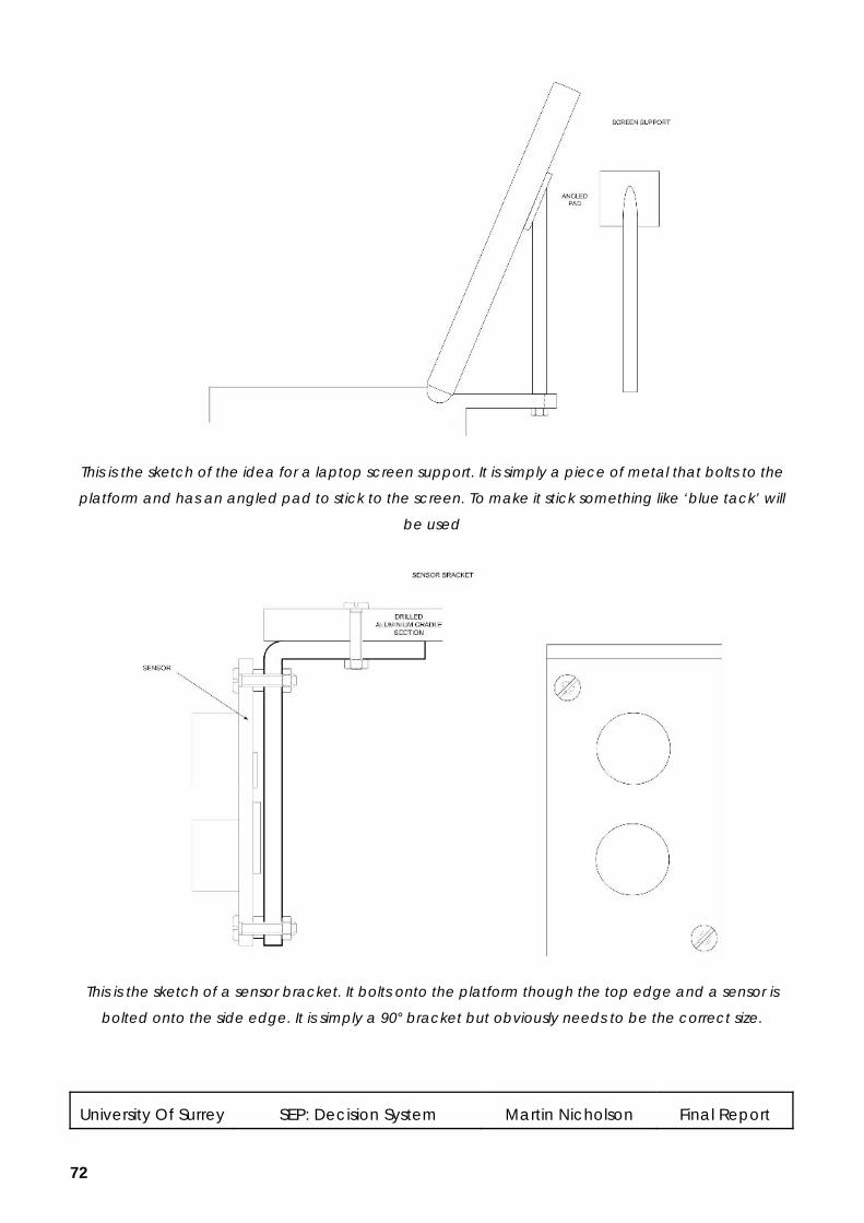
University Of Surrey SEP: Decision System Martin Nicholson Final Report
72
This is the sketch of the idea for a laptop screen support. It is simply a piece of metal that bolts to the
platform and has an angled pad to stick to the screen. To make it stick something like ‘blue tack’ will
be used
This is the sketch of a sensor bracket. It bolts onto the platform though the top edge and a sensor is
bolted onto the side edge. It is simply a 90° bracket but obviously needs to be the correct size.