JOURNAL OF MATHEMATICAL ANALYSIS AND APPLICATIONS 128, 443455 (1987)

Sensitivity Techniques for Systems with Distributed Parameters

VADIM KOMKOV*.+

Department of Mathematics, Winthrop College, Rockhill, North Carolina 29733

Submitted by C. L. Dolph

Received July 3, 1986

We derive a simple sensitivity formula for systems described by the equation Y&U = q, where LZ’ is a partial differential operator that depends on a vector of parameters h. The applications of the formula suggests that different functional analytic settings may offer computational ditliculties and analytical advantages and vice versa. c 1987 Academic Press, Inc.

1. STATEMENT OF THE PROBLEM AND

A PROPOSED FUNCTIONAL ANALYTIC SETTING

The main difficulty in the design and numerical computation of sen- sitivity for an engineering system is the step that involves the computation of the state of the system for a given (intermediate) design which needs to be improved. Typically in iterative techniques suggested by many authors that involve some version of the gradient-projection method, one needs to compute the sensitivity of the state function with respect to some design variables at each iterative step in the design improvement loop. In realistic CAD (computer assisted design) procedures involving the design of a com- plex engineering system this is a very nasty part of the program, causing lengthy computations, excessive roundoff errors and possible errors that may be hard to detect.

Several efforts to bypass this step are mentioned in this paper. These include the so-called Haug-Komkov “trick” or similar adjoint equation approaches.

In this paper we point out that knowledge of the Green’s function or of an elementary solution, that is, of the convolutional inverse of Y, permits an almost trivial computation of the elusive sensitivity term.

* This research was supported by the National Science Foundation under Grant DMC 84-16155.

+ Present address: Department of Mathematics, Air Force Institute of Technology, WPAFB, Ohio 45433.

443 0022-247X/8? $3.00

Copyright ‘c> 1987 by Academic Press, Inc. All rights of reproduction tn any iorm reserved

444 VADIM KOMKOV

Let u represent the state of the system and h a vector of (distributed) design parameters. The design problem consists of improving the value of a functional J(u(h), h, x) subject to some constraints x,(t/,(/z), x) ,< 0, or xZ = 0. The state equation 9~ -q(x) =0 may be regarded as one of the constraints.

The functional analytic setting is generally a Sobolev space H’, i.e., w E H’; h may be a vector in 9’, or some Hilbert or only Banach space. Generally h(x) has a compact support. 9 is generally a linear (or perhaps quasilinear) partial differential operator 9: u -+ Ypu = C ai D’u, Ii1 < m, the coefficients a,(x) are real C” functions. The domain of u is an open set 52 c R”. Some smoothness conditions are specified for 352, which is the boundary of Q. q(x) is an element of Sobolev space HI-“‘, where m is the order of Y. This is the most commonly accepted setting for this type of optimization problem.

As an alternative, one could consider the setting of Mikusinski’s field *M. As in his theory of operators [ 11, one could start with Y,(Q) functions and enlarge the 9,(,(n) algebra with the usual addition (+ ) and convolution (*) operation as the multiplication to a unique field *A4 (see [ 1, Chap. l] for details). Some very serious difficulties arise in manipulating this algebra if both convolution products and pointwise multiplications of functions occur in such formulations simultaneously.

Another difficulty is easily discovered: Only some differential operators can be written as convolutions. d/dx is equivalent to (6’(x)*) in the follow- ing sense: for any W(X) E C’(Q), (d/dx)u = 6’(x) * U(X). However, differen- tial operators with variable coefficients cannot be routinely regarded as elements of *M.

For example, application of the operator x(3/3x) to an arbitrary function f (which is an element of *M) cannot be written in the form CI * f: If this were possible, then the commutative and associative properties of multiplication in *M would imply (m * f) * g = (f * a) * g = f * (a * g) for any g. However, (a * x,) * x: = (x(?I/Jx))x+ * x: =x4,/12, while b+ *.,*x2+=x+ * (x(8/8x)x:)=x4,/6. The difficulty can be traced to non-commutativity of ordinary multiplication and convolution. This can be checked if one applies the Fourier transform to the expression (f* 9g) - (dipf * g), which must vanish for all J g, 9 E *M, if Y is a convolution operator, that is, if the application of 9 to any function f’can be replaced by CI * f for some c1 E *M.

2. DISCUSSION OF SENSITIVITY

The crucial operation is establishing the sensitivity of some vector XE H that depends on h, which is also a vector in a space H,. Let h, be some

SENSITIVITY TECHNIQUES 445

admissible value of h. Let q be a vector in H,, and E a scalar (real number). We call the vector y, E H, the Gateaux difference for X in the direction of Y) if y, is of the form yV = X(h, + EV) - X(/I,,).

We assume that H2 is a normed space. If lim,,, (y,/lls~ll) exists (in H,) we can refer to it as the derivative of X with respect to h in the direction of 17. Mathematically this may be satisfactory; physically it is not. The physical dimension of dX/dh should not be the same as the dimension of X, unless h is a dimensionless quantity.

A more satisfactory definition is X,(q) E 9’( H,, H,)X,,: q -+ y,. If for a given q such a linear map can be established for each admissible vector h in a sufficiently small neighborhood of h,, then X,,(q) is a linear transfor- mation assigning to the vector q E H2 a unique vector y, in H,. Let ho -I- EV be admissible for a small I&(.

Thus, if y, = X(h, + EV) - X(h,) can be written as y, = (X,(r)), q) + O(E’)E H,, with VE H,, X,(q): H, -+ H,, then q is called an admissible direction, and we have a much more satisfactory physical inter- pretation. For example, if X(h) is a functional, X(h) E R and h is an element of a Banach space B, then X,(q) is an element of B* (the dual of B).

If X,(r)) is independent of q, that is, y, =(X,,, q) + o(s2), or y, = (X,, q) + i(q), where Ili(~)ll/lel + 0 as 1~1 --* 0, then we shall refer to X, as the Frechet derivative of X with respect to h computed at h,. There is no reason why X cannot be an operator, where all admissible operators (con- taining X as an element) form some abstract normed space. If the operator Y ,,: H, + H, can be written in the form y,,A = (q, A,(h,))+[, where llilI/lel -+ 0 as 1~1 + 0, and the operator Ah is independent of q, then A, will be called the Frtchet derivative of A with respect to h, computed at h,EH2.

In what follows we shall assume that all operators are invertible. Practically, this implies that we stay away from bifurcation phenomena.

2.1. The Sensitivity Formula

We shall derive a simple formula directly deduced from the state equation

Yu=q, (2.1)

where the postulate the appropriate functional spaces and the algebra in *M, as necessary. The set of all admissible inhomogeneous terms must belong both to the space Hk-’ and to *i&4. Similarly, we have to agree on the choice of admissible state functions (call them generalized dis- placements) U(X).

We assume that with such choices Y is an invertible operator. That is, given q there is a unique U, satisfying (2.1), and Hadamard’s well-posedness conditions are satisfied. (The discussion considering generalized inverses for

446 VADIMKOMKOV

ill-posed problems will have to await future research.) The connection between the existence of inverse map 9-l and existence of the Green’s function is readily established. Let the state equation be of the form 9”~ = q, assuming that it can be written as a convolution in *M.

z**=q. (2.la)

The elementary solution e satisfies the convolution equation

where 6 (Dirac delta) is the multiplicative identity in *M. Then

~0=e*q=LT’q.

e is the Green’s function for the problem for certain classes of partial dif- ferential equations. In engineering jargon e is the influence function for problems in structural engineering, and the impulse function in the elec- trical engineering applications.

In the usual engineering notation we double the number of variables, and, write e * q as @(x - 5) * q(t). We need some lemmas to derive the sensitivity function wh.

LEMMA 1. (e*),, = (YP’)h.

Proof: Two operators 1,) lz are equal by definition if they have the same domain D and range B and for any z E DI, = Dl,, I, z = l,z in 9 (see [ 51).

Since any admissible inhomogeneous term q is in the domain of both operators (e*) and (9-l) and for any admissible q we have e * q = dp ~ ‘q, clearly (e*)[ -(Y-l)] = A. Since the class of admissible forces {q2} is in the domain of both e* and 9-l and the range is the corresponding class of admissible displacements we conclude that if the Frechet derivative A, exists, then it must be equal to (e*)* and to (YP’)h.

LEMMA 2.

(Y--)=9;‘.9h .Y-‘. (2.4)

Note. This is an ordinary composition of operators, not a convolution.

Proof. Computation. Since YY-’ = Pip-‘9 = I is the identity operator, we have

Ih = $3 = (YLr’),, = (9h)Lz-’ + Liq9-‘)h

SENSITIVITY TECHNIQUES 441

or

and

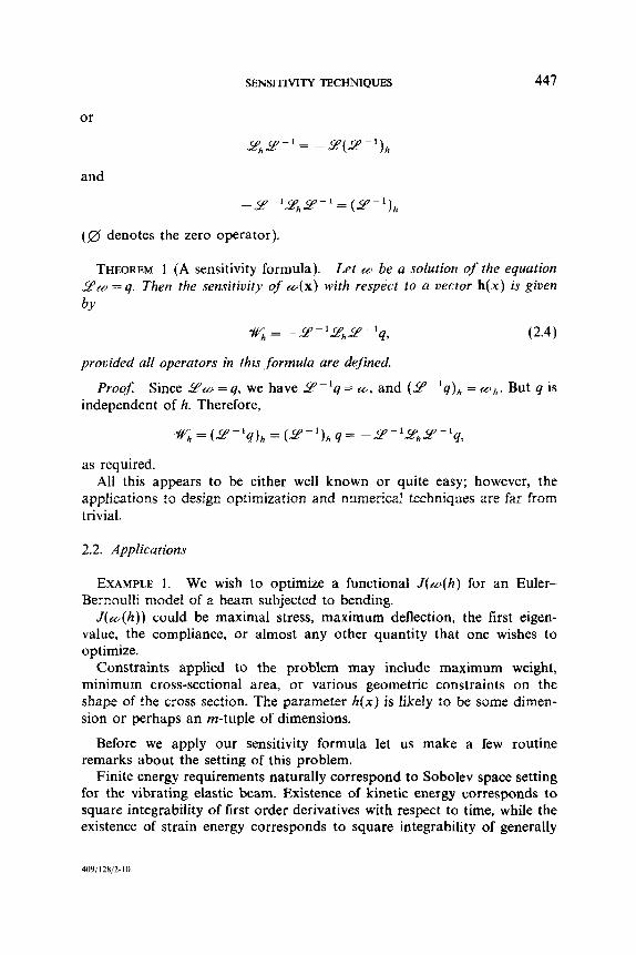
(0 denotes the zero operator).

THEOREM 1 (A sensitivity formula). Let w be a solution of the equation YW = q. Then the sensitivity of W(X) with respect to a vector h(x) is given by

Wh = -z-‘&Y-‘q, (2.4)

provided all operators in this ,formula are defined.

Proof. Since S?SU = q, we have 9’-‘q = CO, and (~?‘q)~ = CCL~. But q is independent of h. Therefore,

as required. All this appears to be either well known or quite easy; however, the

applications to design optimization and numerical techniques are far from trivial.

2.2. Applications

EXAMPLE I. We wish to optimize a functional J(w(h) for an Euler- Bernoulli model of a beam subjected to bending.

J(tu(h)) could be maximal stress, maximum deflection, the first eigen- value, the compliance, or almost any other quantity that one wishes to optimize.

Constraints applied to the problem may include maximum weight, minimum cross-sectional area, or various geometric constraints on the shape of the cross section. The parameter h(x) is likely to be some dimen- sion or perhaps an m-tuple of dimensions.

Before we apply our sensitivity formula let us make a few routine remarks about the setting of this problem.

Finite energy requirements naturally correspond to Sobolev space setting for the vibrating elastic beam. Existence of kinetic energy corresponds to square integrability of first order derivatives with respect to time, while the existence of strain energy corresponds to square integrability of generally

409/128/2-IO

448 VADIM KOMKOV

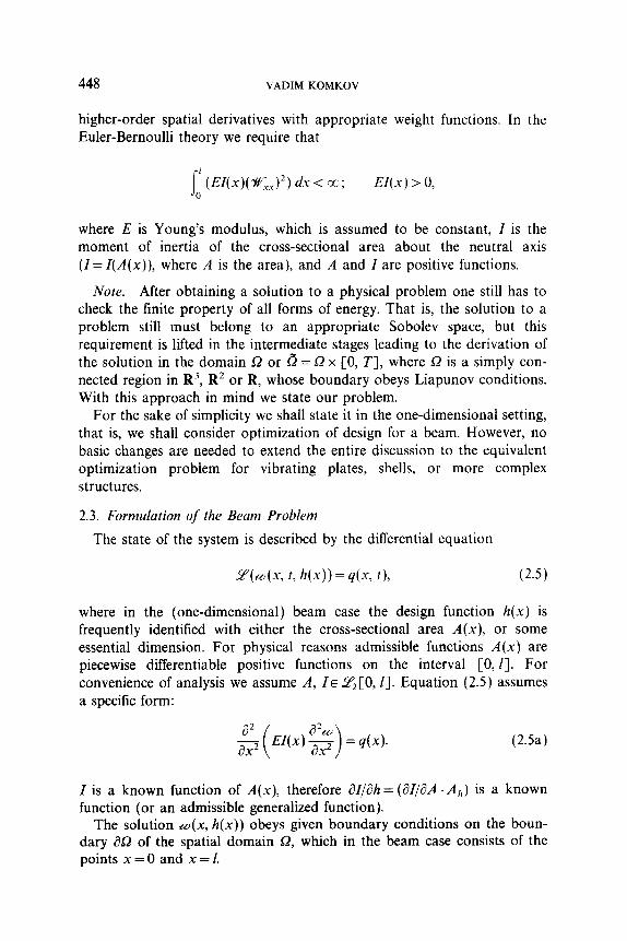
higher-order spatial derivatives with appropriate weight functions. In the Euler-Bernoulli theory we require that

i ’ W(x)(K.d2) dx < 00; EZ( x) > 0, 0

where E is Young’s modulus, which is assumed to be constant, Z is the moment of inertia of the cross-sectional area about the neutral axis (I= Z(A(x)), where A is the area), and A and Z are positive functions.

Note. After obtaining a solution to a physical problem one still has to check the finite property of all forms of energy. That is, the solution to a problem still must belong to an appropriate Sobolev space, but this requirement is lifted in the intermediate stages leading to the derivation of the solution in the domain Q or d = 52 x [0, T], where Q is a simply con- nected region in R3, R* or R, whose boundary obeys Liapunov conditions. With this approach in mind we state our problem.

For the sake of simplicity we shall state it in the one-dimensional setting, that is, we shall consider optimization of design for a beam. However, no basic changes are needed to extend the entire discussion to the equivalent optimization problem for vibrating plates, shells, or more complex structures.

2.3. Formulation of the Beam Problem

The state of the system is described by the differential equation

9(4x, 6 h(x)) = q(x, t), (2.5)

where in the (one-dimensional) beam case the design function h(x) is frequently identified with either the cross-sectional area A(x), or some essential dimension. For physical reasons admissible functions A(x) are piecewise differentiable positive functions on the interval [0, Z]. For convenience of analysis we assume A, ZE &[O, E]. Equation (2.5) assumes a specific form:

(2Sa)

Z is a known function of A(x), therefore dZ/lah = (aZ/aA . Ah) is a known function (or an admissible generalized function).

The solution W(X, h(x)) obeys given boundary conditions on the boun- dary XJ of the spatial domain Q, which in the beam case consists of the points x = 0 and x = 1.

The solutions belong the inner product

SENSITIVITY TECHNIQUES 449

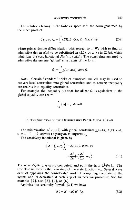
to the Sobolev space with the norm generated by

(~1, Y,), = J, W(x) Y;(x, f) Y% t)) dx> (2.6)

where primes denote differentiation with respect to x. We wish to find an admissible design h(x) to be substituted in (2.5), or A(x) in (2Sa), which minimizes the cost functional J(u(x, t), h(x)). The constraints assigned to admissible designs are “global” constraints of the form

It/j = f’ xj(ti, h(X)) dx < 0.

Note. Certain “standard” tricks of numerical analysis may be used to convert local constraints into global constraints and to convert inequality constraints into equality constraints.

For example, the inequality q(x) 6 0, for all XEQ, is equivalent to the global equality constraint

s R 11~1 +vI dx=O. 3. THE SOLUTION OF THE OPTIMIZATION PROBLEM FOR A BEAM

The minimization of J(u(h) with global constraints ~~(~u(h), h(x), x) < 0, GI = 1, 2, . ..) k, admits Lagrangian mulitpliers 1,.

The sensitivity functional is given by

(3.1)

The term &/ah Iho is easily computed, and so is the term &/a, Ih0. The troublesome term is the derivative of the state function We. Several ways exist of bypassing the considerable work of computing the state of the system and its derivative at each step of an iterative procedure. See, for example, [2], also [3], [4], or [S].

Applying the sensitivity formula (2.4) we have

(3.2)

450 VADIM KOMKOV

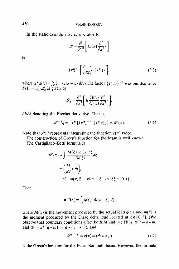
In the static case the inverse operator to

+.+z(x)g.]

(3.3)

where x*+2(x) = s:, 5 + .z(x - 5) dt. (The factor { r( 1 )} ~’ was omitted since r(l) = 1.) Yh is given by

i3Zjah denoting the Frechet derivative. That is,

‘r-q= {x*+[(H-‘.(x*,q)]}=W(x). (3.4)

Note that x:f represents integrating the function f(x) twice. The construction of Green’s function for the beam is well known. The Castigliano-Betti formula is

if 4x, 5) = W - 51, {x, C} E [IO, 11.

Then

w”(x)= j’q(r)+W- 5) &, 0

where M(x) is the movement produced by the actual load q(x), and m(t) is the moment produced by the Dirac delta load located at 5 E [0, Z]. (We observe that boundary conditions affect both M and m.) Thus, %‘“” = q * 2, and W=x*,(q*rfi) = q*(x+ *ti), and

9(‘-‘)=e(x)=(rFz*x+) (3.5)

is the Green’s function for the Euler-Bernoulli beam. However, the formula

SENSITIVITY TECHNIQUES 451

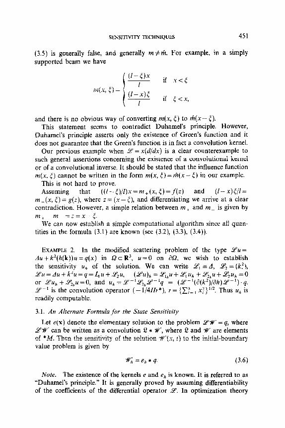
(3.5) is generally false, and generally m # &. For example, in a simply supported beam we have

if x<t

if 5 <x,

and there is no obvious way of converting m(x, 5) to riz(x - 5). This statement seems to contradict Duhamel’s principle. However,

Duhamei’s principle asserts only the existence of Green’s function and it does not guarantee that the Green’s function is in fact a convolution kernel.

Our previous example when 9 = x(d/dx) is a clear counterexample to such general assertions concerning the existence of a convolutional kernel or of a convolutional inverse. It should be stated that the influence function m(x, [) cannot be written in the form m(x, 5)=&(x-0 in our example.

This is not hard to prove. Assuming that ((l-t)/l)x=m+(x, t)=f(z) and (l-x)l/l=

m-(x, 5) = g(z), where z = (x - <), and differentiating we arrive at a clear contradiction. However, a simple relation between m, and m- is given by m, -rn- =z=x-t.

We can now establish a simple computational algorithm since ail quan- tities in the formula (3.1) are known (see (3.2), (3.3), (3.4)).

EXAMPLE 2. In the modified scattering problem of the type 9~ = du+k*(h(k))u=q(x) in QcR3, u = 0 on 852, we wish to establish the sensitivity u,, of the solution. We can write PI =d, 64, = (kz), YU=Llu+k~u=q=z.ju++2U, (~U)h=~~*U+~~;Uh+~~*U+~~Uh=O or Yu, + TZhu = 0, and uh = 2-192hY-1q = (2’-1(d(k2)/8h)9-1) .q. 56’~ I is the convolution operator ( - 1/4Ur*), r = {C?=, xf } ‘I*. Thus u,, is readily computable.

3.1. An Alternate Formula for the State Sensitivity

Let e(x) denote the elementary solution to the problem 5Yw = q, where 5?w can be written as a convolution !i! * “llr, where L? and Y#- are elements of *M. Then the sensitivity of the solution nwI(x, t) to the initial-boundary value problem is given by

6 = eh * q. (3-b)

Note. The existence of the kernels e and eh is known. It is referred to as “Duhamel’s principle.” It is generally proved by assuming differentiability of the coefficients of the differential operator 9. In optimization theory

452 VADIMKOMKOV

such assumption is troublesome, but in the setting of *A4 algebra it is a trivial result if 9 can be represented as a convolution, and it does not require differentiability but only 9’ property of these coefficients. (Even that can be weakened with very little additional effort.) Unfortunately, to the best of my knowledge, the theory concerning *M algebras has not been sufficiently developed to resolve even the simple classification problems.

The following comments should be made. Provided we stay with con- volution algebras and avoid pointwise multiplication several “difficult” problems become quite trivial.

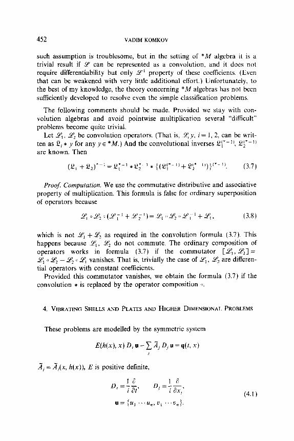
Let YI, Yz be convolution operators. (That is, g. y, i = 1,2, can be writ- ten as 52, * y for any y E *M.) And the convolutional inverses 5Zj*-l), er-‘) are known. Then

(2, +~2)*-Ly *$3-l * {(~‘,‘-l)+~~*~“)}‘*-“. (3.7)

ProoJ Computation. We use the commutative distributive and associative property of multiplication. This formula is false for ordinary superposition of operators because

which is not 9, + L$, as required in the convolution formula (3.7). This happens because Y,, J& do not commute. The ordinary composition of operators works in formula (3.7) if the commutator [Yr , -4p] = YI 0 LZz - LZ’~ o 9, vanishes. That is, trivially the case of 9,) L&l are differen- tial operators with constant coefficients.

Provided this commutator vanishes, we obtain the formula (3.7) if the convolution * is replaced by the operator composition 0.

4. VIBRATING SHELLS AND PLATES AND HIGHER DIMENSIONAL PROBLEMS

These problems are modelled by the symmetric system

E@(x), x) D, u - 1 Aj 0, u = q(t, x)

2, = Aj(x, h(x)), E is positive definite,

D, =fi, D.=LA J i dxj’

(4.1) u= (u, “‘ll,, u, . ..v.}

SENSITIVITY TECHNIQUES

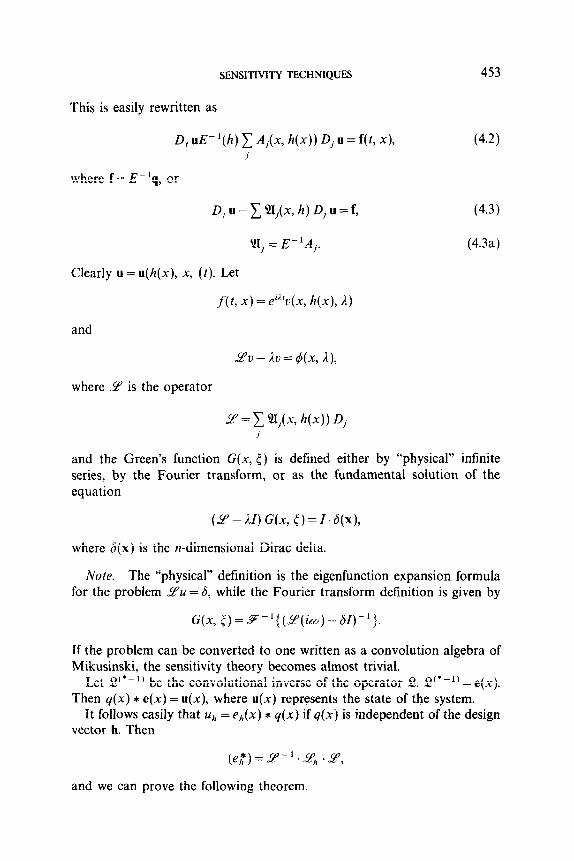
This is easily rewritten as

D, UE-‘(II) C Aj(X, h(X)) DjU=f(t, X),

where f = E- ‘q, or

D,u-x21j(x,h)Dju=f,

91j = E-44,.

Clearly u = u(k(x), x, (t). Let

f(t, x) = e’“‘o(x, h(x), 1)

and

9u - ill = qqx, A),

where 9 is the operator

~=C cui(X, h(X))Dj

453

(4.2)

(4.3)

(4.3a)

and the Green’s function G(x, <) is defined either by “physical” infinite series, by the Fourier transform, or as the fundamental solution of the equation

(9 - LZ) G(x, 5) = Z.~(X),

where 6(x) is the n-dimensional Dirac delta.

Note. The “physical” definition is the eigenfunction expansion formula for the problem YU = 6, while the Fourier transform definition is given by

G(x, ()=S-‘{(~(iu+61)-‘1.

If the problem can be converted to one written as a convolution algebra of Mikusinski, the sensitivity theory becomes almost trivial.

Let !2(*-‘) be the convolutional inverse of the operator 2. f?(‘-‘) = e(x). Then q(x) * e(x) = u(x), where u(x) represents the state of the system.

It follows easily that u,, = eh(x) * q(x) if q(x) is independent of the design vector h. Then

and we can prove the following theorem.

454 VADIMKOMKOV

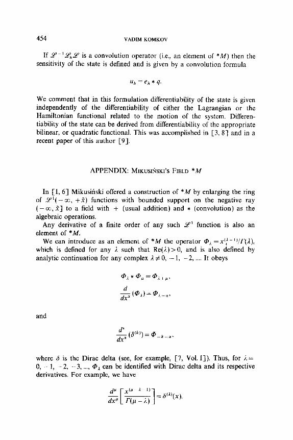
If T-‘phg is a convolution operator (i.e., an element of *M) then the sensitivity of the state is defined and is given by a convolution formula

uh = eh * q.

We comment that in this formulation differentiability of the state is given independently of the differentiability of either the Lagrangian or the Hamiltonian functional related to the motion of the system. Differen- tiability of the state can be derived from differentiability of the appropriate bilinear, or quadratic functional. This was accomplished in [3, S] and in a recent paper of this author [9].

APPENDIX: MIKUSII~SKI'S FIELD *A4

In [ 1, 61 Mikusinski offered a construction of *A4 by enlarging the ring of .Y’( - co, +Z) functions with bounded support on the negative ray (-co, Z] to a field with + (usual addition) and * (convolution) as the algebraic operations.

Any derivative of a finite order of any such 2’ function is also an element of *M.

We can introduce as an element of *M the operator Q1 = xy- ‘)/r(J), which is defined for any I such that Re(l)>O, and is also defined by analytic continuation for any complex ,J # 0, - 1, - 2, . . . It obeys

$ (@A)=@i.--cry

and

-g (W) = @-La.

where 6 is the Dirac delta (see, for example, [7, Vol. I]). Thus, for 1= 0, -1, -2, -3, . ..) @A can be identified with Dirac delta and its respective derivatives. For example, we have

SENSITIVITY TECHNIQUES 455

REFERENCES

1. J. MIKUSIP~SKI, “The Theory of Operators,” PAN Warsaw, 1957. 2. E. J. HAUC AND V. KOMKOV, Sensitivity analysis in distributed parameter mechanical

systems optimization, J. Optim. Theory Appl. 23, No. 3 (1977), 445464. 3. E. J. HAUG, K. CHOI, AND V. KOMKOV, “Design Sensitivity of Structural Systems,”

Academic Press, New York, 1986. 4. V. KOMKOV, “Variational Principles of Continuum Mechanics,” Reidel, Dordrecht, 1986. 5. R. A. ADAMS, “Sobolev Spaces,” Academic Press, New York, 1975. 6. J. MIKUSIASKI, Lectures on constructive theory of distributions, lecture notes, University of

Florida, Gainesville, FL, 1969. 7. I. M. GELFAND AND G. E. SHILOV, “Generalized Functions,” Vol I, Academic Press,

New York/London, 1964. 8. B. ROUSSELET AND E. J. HAUG, Design sensitivity in structural mechanics. III. Effects of

shape vibration, J. Sfructural Mech. 10 No. 3 (1982) 273-310. 9. V. KOMKOV, Properties of the sensitivity function, Arch. Mech. (Arch. Mech. Stos.), in

press.