SENSITIVITY OF SWEPT-WING BOUNDARY-LAYER TRANSITION TO

SPANWISE-PERIODIC DISCRETE ROUGHNESS ELEMENTS

A Thesis

by

DAVID EDWARD WEST

Submitted to the Office of Graduate and Professional Studies of

Texas AampM University

in partial fulfillment of the requirements for the degree of

MASTER OF SCIENCE

Chair of Committee William S Saric

Committee Members Helen L Reed

David A Staack

Head of Department Rodney D W Bowersox

December 2014

Major Subject Aerospace Engineering

Copyright 2014 David Edward West

ii

ABSTRACT

Micron-sized spanwise-periodic discrete roughness elements (DREs) were applied to

and tested on a 30deg swept-wing model in order to study their effects on boundary-layer

transition in flight where stationary crossflow waves are the dominant instability

Significant improvements have been made to previous flight experiments in order to more

reliably determine and control the model angle of attack (AoA) and unit Reynolds number

(Reprime) These improvements will aid in determining the influence that DREs have on swept-

wing laminar-turbulent transition Two interchangeable leading-edge surface-roughness

configurations were tested polished and painted The baseline transition location for the

painted leading edge (increased surface roughness) was unexpectedly farther aft than the

polished Transport unit Reynolds numbers were achieved using a Cessna O-2A

Skymaster Infrared thermography coupled with a post-processing code was used to

globally extract a quantitative boundary-layer transition location Each DRE configuration

was compared to curve-fitted baseline data in order to determine increases or decreases in

percent laminar flow while accounting for the influence of small differences in Re and

AoA Linear Stability Theory (LST) guided the DRE configuration test matrix In total 63

flights were completed where only 30 of those flights resulted in useable data While the

results of this research have not reliably confirmed the use of DREs as a viable laminar

flow control technique in the flight environment it has become clear that significant

computational studies specifically direct numerical simulation (DNS) of these particular

iii

DRE configurations and flight conditions are a necessity in order to better understand the

influence that DREs have on laminar-turbulent transition

iv

DEDICATION

This work is dedicated to my wife and best friend Rebecca Her continual support

optimism and love have helped me endeavor through my education with a sense of

determination and enthusiasm

v

ACKNOWLEDGEMENTS

This research effort was the culmination of several contributors through funding

advisement corroboration motivation and encouragement It is because of these people

and their contributions that this research was possible Funding for this effort was provided

by the National Aeronautics and Space Administration (NASA) through Analytical

Mechanics Associates Inc (AMA-Inc) and by Air Force Research Laboratories (AFRL)

at Wright-Patterson Air Force Base (WPAFB) through General Dynamics IT

I would first like to thank Dr William Saric for providing me the opportunity

advisement and encouragement needed to accomplish this research effort Before I entered

graduate school at Texas AampM University Dr Saric brought me on as an undergraduate

research assistant at the Klebanoff-Saric Wind Tunnel (KSWT) where my interest in

research was first cultivated and developed Upon graduation I was afforded the

opportunity to work at the Flight Research Lab as an engineering associate where my

desire to pursue a graduate degree really took hold Now looking back Irsquom greatly

appreciative for the four-plus years of guidance and wisdom that Dr Saric provided me I

know that laminar flow control using DREs has been a passion and investment for Dr

Saric and I am honored to be a small part of the research process I donrsquot take lightly the

trust that he put in me to conduct a worthwhile experiment I would also like to thank my

graduate committee members (both current and former) Dr Helen Reed Dr David Staack

and Dr Devesh Ranjan for their guidance and support throughout this research endeavor

They were always willing to assist when needed and offer suggestions for the success of

vi

my work Irsquod also like to thank our program specialists Colleen Leatherman and Rebecca

Mariano for their logistical support of both my research and that of the Aerospace

Engineering Department Without their experience and willingness to exceed

expectations our research team would never come close to the efficiency and productivity

it now enjoys

While completing this research I had the opportunity to work with several graduate

and undergraduate students who contributed so much to the success of this effort Most of

all I would like to thank Brian Crawford and Dr Tom Duncan These two extremely

dedicated and hard-working colleagues have supported me throughout my entire graduate

career at Texas AampM Without their skills experience and expertise this research would

never have had the amount of quality sophistication and attention to detail it needed to be

successful From model design instrumentation development data acquisition amp

processing and flight crew support these young men have truly shown their dedication to

research and to myself I wholeheartedly consider them more than just colleagues or class-

mates but as genuinely devoted friends Additionally Matthew Tufts provided all of the

computational support for this research effort and also showed me continual support and

friendship Every good experiment has a computational counterpart and his was

exemplary I would also like to acknowledge the following former students who helped

develop my skills as a researcher throughout my undergraduate and graduate career Dr

Lauren Hunt Dr Rob Downs and Dr Matthew Kuester Also I would like to

acknowledge the following students (both former and current) for their support of this

research by assisting with flight crew duties of co-pilot and ground crew Dr Jacob

vii

Cooper Colin Cox Alex Craig Brian Crawford Dr Rob Downs Dr Tom Duncan

Kristin Ehrhardt Dr Bobby Ehrmann Joshua Fanning Simon Hedderman Kevin

Hernandez Heather Kostak Dr Matthew Kuester Erica Lovig Dr Chi Mai Ian Neel

Matthew Tufts and Thomas Williams

The test pilots who contributed to this research include both Lee Denham and Lt Col

Aaron Tucker PhD I would like to thank both of them for their talent continual dedication

and expertise which helped make these experiments both safe and successful They were

always available for early mornings and made it a point to bring a professional and

accommodating attitude to every flight Additionally these experiments would not be

possible without the diligence and proficiency of our AampP mechanic Cecil Rhodes Cecil

continually and reliably maintained the aircraft to ensure the safety of every flight

Moreover he provided extensive knowledge and training for myself and other students in

the areas of mechanics sheet metal work woodworking milling and painting

Finally I would like to thank my family for their perpetual support and prayers

throughout my career as a student I thank my parents Jim and Linda West who always

encouraged me to do my best and to be proud of my accomplishments without them I

would not have been able to call myself a proud Aggie Irsquod also like to thank my wife

Rebecca to whom this work is dedicated and who was and is always there for me

viii

NOMENCLATURE

5HP five-hole probe

A total disturbance amplitude

Ao reference total disturbance amplitude baseline at xc = 005

AMA-Inc Analytical Mechanics Associates Inc

AoA angle of attack

ASU Arizona State University

BCF baseline curve fit

c chord length 1372 m

Cp3D coefficient of pressure

CO Carbon Monoxide

DAQ data acquisition

DBD dielectric-barrier discharge

DFRC Dryden Flight Research Center

DNS direct numerical simulation

DREs spanwise-periodic discrete roughness elements

DTC digital temperature compensation

FRL Flight Research Laboratory (Texas AampM University)

FTE flight-test engineer

GTOW gross take-off weight

HP horse power

ix

IR infrared

k step height forward-facing (+) aft-facing (-)

KIAS knots indicated airspeed

KSWT Klebanoff-Saric Wind Tunnel (Texas AampM University)

LabVIEW Laboratory Virtual Instrument Engineering Workbench

(data acquisition software)

LE leading edge

LFC laminar flow control

LIDAR Light Detection And Ranging

LST Linear Stability Theory

M Mach number

MSL mean sea level

N experimental amplification factor (natural log amplitude ratio

from LST)

Neff Effective N-Factor (depends on DRE xc placement)

Nmax maximum N-Factor possible for specific wavelength

Ntr transition N-Factor (N at xc transition location)

NASA National Aeronautics and Space Administration

NPSE Nonlinear Parabolized Stability Equation

NTS non-test surface

OML outer mold line

x

ONERA Office National dEacutetudes et de Recherches Aeacuterospatiales

(French aerospace research center)

P2P Pixels 2 Press (DRE manufacturing company)

PDF probability density function

PID proportional integral derivative (a type of controller)

Pk-Pk peak-to-peak

PSD power spectral density

ps freestream static pressure

q dynamic pressure

Reʹ unit Reynolds number

Rec chord Reynolds number

ReθAL attachment-line momentum-thickness Reynolds number

RMS root mean square

RMSE root mean square error

RTD resistance temperature detector

RTV room temperature vulcanizing

s span length of test article 1067 m

S3F Surface Stress Sensitive Film

std standard deviation of the measurement

SWIFT Swept-Wing In-Flight Testing (test-article acronym)

SWIFTER Swept-Wing In-Flight Testing Excrescence Research

(test-article acronym)

xi

T temperature

TAMU-FRL Texas AampM University Flight Research Laboratory

TEC thermoelectric cooler

TLP traversing laser profilometer

TRL technology readiness level

T-S Tollmien-Schlichting boundary-layer instability

Tu freestream turbulence intensity

Uinfin freestream velocity

VFR visual flight rules

VI virtual instrument (LabVIEW file)

WPAFB Wright-Patterson Air Force Base

x y z model-fixed coordinates leading-edge normal wall-normal

leading-edge-parallel root to tip

xt yt zt tangential coordinates to inviscid streamline

X Y Z aircraft coordinates roll axis (towards nose) pitch axis (towards

starboard) yaw axis (towards bottom of aircraft)

xtrDRE streamwise transition location with DREs applied

xtrbaseline streamwise transition location of the baseline (no DREs)

α model angle of attack

αoffset chord-line angle offset (5HP relative to test article)

β aircraft sideslip angle

βoffset yaw angle that the test-article is offset from the aircraft centerline

xii

δ99 boundary-layer thickness at which uUedge = 099

ΔLF percent-change in laminar flow

θ boundary-layer momentum thickness

θAC pitch angle of aircraft

θACoffset aircraft-pitch angle offset (5HP relative to test article)

120582 wavelength

Λ leading-edge sweep angle

σBCF baseline curve fit uncertainty

σΔLF percent-change in laminar flow uncertainty

xiii

TABLE OF CONTENTS

Page

ABSTRACT ii

DEDICATION iv

ACKNOWLEDGEMENTS v

NOMENCLATURE viii

TABLE OF CONTENTS xiii

LIST OF FIGURES xv

LIST OF TABLES xviii

1 INTRODUCTION 1

11 Motivation 1 12 Swept-Wing Boundary-Layer Stability and Transition 3 13 Previous Experiments 10 14 Experimental Objectives 13

2 IMPROVEMENTS TO PREVIOUS TAMU-FRL DRE EXPERIMENTS 15

21 Flight Research Laboratory 15 22 Overview and Comparison of SWIFT and SWIFTER 19 23 Five-Hole Probe and Calibration 23 24 Infrared Thermography 28 25 Traversing Laser Profilometer 39

3 EXPERIMENTAL CONFIGURATION AND PROCEDURES 42

31 Experimental Set-up Test Procedures and Flight Profile 42 32 Surface Roughness 48 33 Linear Stability Theory 55 34 Spanwise-Periodic Discrete Roughness Elements 57

4 RESULTS 64

41 Infrared Thermography Transition Data 65 42 Baseline Curve Fit 68 43 Percent-Change in Laminar Flow Data 73

xiv

5 SUMMARY CONCLUSIONS AND RECOMMENDATIONS 84

51 Flight-Test Summary 84 52 Future Research Recommendations 85

REFERENCES 88

APPENDIX A PERCENT LAMINAR FLOW FIGURES 94

APPENDIX B SWIFTER OML AND COEFFICIENT OF PRESSURE DATA 116

APPENDIX C POST-PROCESSED INFRARED THERMOGRAPHY FIGURES 118

xv

LIST OF FIGURES

Page

Fig 1 Transition paths from receptivity to breakdown and turbulence

(modified figure from Saric et al 2002 [4]) 4

Fig 2 Inviscid streamline for flow over a swept wing 6

Fig 3 Crossflow boundary-layer profile (Saric et al 2003 [10]) 6

Fig 4 Crossflow streaking observed through naphthalene flow visualization 8

Fig 5 Co-rotating crossflow vortices 8

Fig 6 Raw infrared thermography image of a saw-tooth crossflow transition

front 10

Fig 7 Stemme S10-V (left) and Cessna O-2A Skymaster (right) hangared at

TAMU-FRL 16

Fig 8 Dimensioned and detailed three-view drawing of the Cessna O-2A

Skymaster 18

Fig 9 SWIFTER and hotwire sting mount attached to the port and starboard

wings of the Cessna O-2A Skymaster respectively (Photo Credit

Jarrod Wilkening) 20

Fig 10 SWIFT (left) amp SWIFTER (right) side-by-side 21

Fig 11 SWIFTER airfoil graphic (top) and LE actuation system (bottom)

(modified figure from Duncan 2014 [32]) 23

Fig 12 Five-hole probe (5HP) freestream static ring (left) conical tip

(middle) pressure port schematic (right) 24

Fig 13 SWIFT five-hole probe mount 25

Fig 14 SWIFTER five-hole probe mount 26

Fig 15 Temperature controlled pressure transducer box 27

Fig 16 SWIFTER heating sheet layout Blue heating wire Red RTV silicone

Insulation and reference RTD not pictured 30

xvi

Fig 17 Idealized graphic of wall heated model (not to scale) (top)

Temperature distribution near transition (bottom) (Crawford et al

2013 [35]) 32

Fig 18 Raw IR image from SWIFT model with qualitative transition front

detection at 50 chord (modified figure from Carpenter (2009) [14]) 35

Fig 19 Raw IR image from SWIFTER model with qualitative transition front

detection at 35-40 35

Fig 20 Comparison of raw (left) and processed (right) IR images 37

Fig 21 Raw IR image overlaid on SWIFTER model in flight 37

Fig 22 Traversing Laser Profilometer with labeled components (modified

figure from Crawford et al 2014b [37]) 41

Fig 23 SWIFTER and SWIFT szligoffset schematic (angles are exaggerated for

visualization purposes) (modified figure from Duncan (2014) [32]) 43

Fig 24 Instrumentation layout in rear of O-2A cabin (Duncan 2014 [32]) 44

Fig 25 Typical flight profile 47

Fig 26 Typical Reprime and α traces while on condtion 47

Fig 27 SWIFT surface roughness spectrogram of painted LE Data taken

using the TLP 49

Fig 28 SWIFTER model in flight with polished (left) and painted (right) LE

installed 50

Fig 29 SWIFTER LE being measured with the TLP 51

Fig 30 Wooden LE stand for traversing laser profilometer measurements 52

Fig 31 SWIFTER painted LE spectra for xc = -0004 ndash 0004 (-04 to 04

chord) 53

Fig 32 SWIFTER painted LE spectra for xc = 0005 ndash 0077 (05 to 77

chord) 54

Fig 33 SWIFTER painted LE spectra for xc = 0067 ndash 0146 (67 to 150

chord) 54

Fig 34 N-Factor plot for SWIFTER at α = -65deg and Reprime = 55 x 106m The

plot on the right is a zoomed in version of the plot on the left 56

Fig 35 3-D scan of Pixels 2 Press DREs spaced at 225 mm 59

xvii

Fig 36 DRE application photos constant chord markers (left) DRE amp

monofilament alignment (right) 60

Fig 37 Example post-processed IR image 66

Fig 38 Direct IR comparison between baseline flight 862 (left) and DRE

flight 863 (right) with target conditions of α = -65deg amp Reprime = 570 x

106m [12microm|225mm|1mm|230|02-14] 68

Fig 39 Baseline-transition surface fit for polished leading edge 69

Fig 40 Baseline-transition surface fit for painted leading edge 70

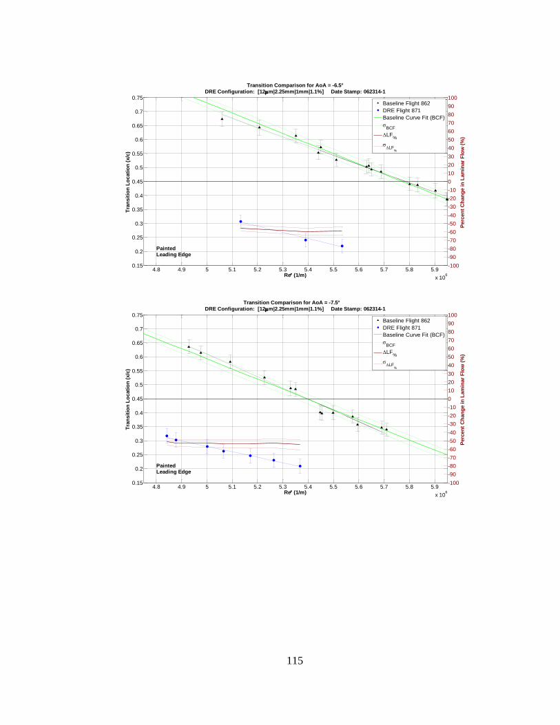
Fig 41 Baseline transition comparison for α = -65deg 71

Fig 42 Baseline transition comparison for α = -75deg 72

Fig 43 DRE flight 871 transition comparison for α = -65deg 74

Fig 44 DRE flight 871 transition comparison for α = -75deg 75

Fig 45 Direct IR comparison between baseline flight 862 (left) and DRE

flight 871 (right) with target conditions of α = -65deg amp Reprime = 550 x

106m [12microm|225mm|1mm|110|11-13] 76

Fig 46 Direct IR comparison between baseline flight 862 (left) and DRE

flight 871 (right) with target conditions of α = -75deg amp Reprime = 530 x

106m [12microm|225mm|1mm|110|11-13] 77

Fig 47 DRE flight 847 transition comparison for α = -65deg 78

Fig 48 DRE flight 847 transition comparison for α = -75deg 79

Fig 49 DRE flight 870 transition comparison for α = -65deg 79

Fig 50 DRE flight 870 transition comparison for α = -75deg 80

Fig 51 DRE flight 829 transition comparison for α = -65deg 81

Fig 52 DRE flight 829 transition comparison for α = -75deg 81

Fig 53 DRE flight 840 transition comparison for α = -75deg 82

Fig 54 DRE flight 865 transition comparison for α = -75deg 82

xviii

LIST OF TABLES

Page

Table 1 Cessna O-2A Specifications 19

Table 2 RMSE and Pk-Pk values of the 5HP calibration (modified table from

Duncan 2014 [32]) 28

Table 3 Effective N-Factor Chart for SWIFTER at α = -65deg amp Reprime = 55 x

106m 57

Table 4 DRE configurations tested on the polished LE 62

Table 5 DRE configurations tested on the painted LE 63

1

1 INTRODUCTION

This thesis describes characterizes and reviews the experimental research on the

feasibility of using spanwise-periodic discrete roughness elements (DREs) as a reliable

and consistent means of swept-wing laminar flow control in the flight environment These

experiments are a continuation of numerous efforts aimed at delaying laminar-turbulent

transition at the Texas AampM University Flight Research Laboratory (TAMU-FRL)

This introduction encapsulates the motivation for laminar-flow control the theory

behind transition instabilities previous experiments showing the development of DREs as

a control technique and finally the objectives this research hopes to achieve Significant

emphasis is placed upon improvements to previous DRE experiments so as to more

reliably determine the sensitivity of laminar-turbulent transition to DREs in flight The

experimental methods procedures and results are enumerated and documented along with

final overview discussion and summary Concurrent computational support was provided

by Matthew Tufts a doctoral candidate in the Aerospace Engineering department at Texas

AampM University

11 Motivation

Enhancing aircraft efficiency is currently and will continue to be a top priority for

military commercial and general aviation Specifically aircraft efficiency can be gained

by reducing skin friction drag which for a commercial transport aircraft represents about

50 of the total drag (Arnal amp Archambaud 2009 [1]) A viable option for drag reduction

2

is through laminar flow control (LFC) or more specifically the delaying of

laminar-turbulent boundary-layer transition Sustained laminar flow over 50 of a

transport aircraftrsquos wings tail surfaces and nacelles could result in an overall drag

reduction of 15 (Arnal amp Archambaud 2009 [1]) A direct benefit of drag reduction

includes lower specific fuel consumption which translates directly into increased range

heavier payloads or overall lower operating costs

Controlling laminar-turbulent boundary-layer transition can be accomplished through

either active and passive methods or a hybrid of the two These methods can include

suction near the leading edge reduction of leading edge surface roughness unsweeping

the leading edge to something less than 20ordm or even through the use of DREs applied near

the attachment line of a swept wing (Saric et al 2011 [2]) DREs in particular are aimed

at delaying transition by controlling the crossflow instability Over the course of

approximately eighteen years DREs have been tested in both wind tunnels and in the

flight environment at compressibility conditions ranging from subsonic to supersonic

Throughout these experiments DREs have been implemented in an assortment of ways

that vary widely in shape size application and operation however all variants are

intended to serve the same fundamental purpose of controlling crossflow The three

principal types of DREs include appliqueacute pneumatic and dielectric-barrier discharge

(DBD) plasma actuators Although pneumatic and plasma techniques can have a variable

amplitude and distribution and in principle be active in this thesis they are considered to

be passive

3

DRE configurations that have successfully delayed laminar-turbulent transition are

almost exclusively found in wind tunnel experiments while the flight environment has

achieved only limited success eg Saric et al (2004) [3] In order to broaden the

understanding implementation and utilization of DREs as a viable LFC technique it is

crucial to both quantify the sensitivity of transition to DREs and to repeatedly demonstrate

delayed transition in the flight environment

12 Swept-Wing Boundary-Layer Stability and Transition

As stated earlier DREs are specifically designed to delay boundary-layer transition by

controlling the crossflow instability however crossflow is not the only instability

mechanism that can lead to breakdown and transition to turbulence Swept wings in

particular are susceptible to four major instabilities including Tollmien-Schlichting (T-S)

(streamwise) crossflow attachment-line and Goumlrtler (centrifugal) instabilities Transition

to turbulence can occur through one of these major instabilities because unstable

disturbances grow within the boundary layer In order to focus on controlling only

crossflow the other three instabilities must be suppressed or precluded through airfoil amp

wing design Before discussing methods of suppression it is important to briefly describe

the receptivity process and each of the instabilities with a more inclusive focus on

crossflow

Receptivity and Swept-Wing Instabilities

Receptivity is essentially the process through which freestream disturbances enter the

boundary layer as steady andor unsteady fluctuations which then interact with the surface

characteristics of a wingairfoil Receptivity establishes the initial conditions of

4

disturbance amplitude frequency and phase for the breakdown of laminar flow (Saric et

al 2002 [4]) While there are several paths from receptivity to breakdown and turbulence

as shown in Fig 1 this research focuses on path A Path A is the traditional avenue for

low disturbance environments where modal growth is significant and transient growth is

insignificant Morkovin (1969) [5] Morkovin et al (1994) [6] Saric et al (2002) [4] and

Hunt (2011) [7] provide a more complete description of the process and the different paths

to breakdown

Fig 1 Transition paths from receptivity to breakdown and turbulence (modified figure from Saric

et al 2002 [4])

The Tollmien-Schlichting instability colloquially referred to as T-S waves is a

streamwise instability that occurs in two-dimensional flows and at the mid-chord region

of swept wings This instability is driven by viscous effects at the surface and often occurs

due to a local suction peak or a decelerating boundary layer Accelerating pressure

Receptivity

Forcing Environmental Disturbances

Transient Growth

Primary Modes

Secondary Mechanisms

Breakdown

Turbulence

Bypass

increasing amplitude

A B C D E

5

gradients are the basis for all natural LFC airfoils that are subject to T-S waves because

T-S waves are stabilized by favorable pressure gradients

Attachment-line instabilities and leading-edge contamination even though they are

different phenomena are both typically inherent to swept wings If the boundary layer at

the attachment line on a swept wing becomes turbulent either due to leading-edge radius

design or contamination from another source then the turbulence can propagate along the

attachment line and contaminate the boundary layer on both wing surfaces aft of the initial

entrained disturbance It is generally accepted that the solution to this particular instability

and contamination is to design your swept wing such that the attachment-line momentum-

thickness Reynolds number ReθAL is kept below the critical value of approximately 100

(Pfenninger 1977 [8])

The Goumlrtler instability is a wall-curvature-induced counter-rotating centrifugal

instability that is aligned with the streamlines (Saric 1994 [9]) It is often referred to as a

centrifugal instability and is caused by a bounded shear flow over a concave surface This

instability is easily eliminated by avoiding any concave curvature before the pressure

minimum on a swept wing

Finally the crossflow instability found in three-dimensional boundary layers develops

as a result of wing sweep coupled with pressure gradient This coupled interaction between

wing sweep and pressure gradient produces curved streamlines at the edge of the boundary

layer as depicted in Fig 2 Inside the boundary layer the streamwise velocity decreases

to zero at the wall but the pressure gradient remains unchanged This imbalance of

centripetal acceleration and pressure gradient produces a secondary flow that is

6

perpendicular to the inviscid streamline called the crossflow component The crossflow

component of the 3-D boundary layer must be zero at both the wall and the boundary-

layer edge producing an inflection point in the profile This inflection point is well known

to be an instability mechanism Fig 3 shows the resultant crossflow boundary-layer profile

along with its components

Fig 2 Inviscid streamline for flow over a swept wing

Fig 3 Crossflow boundary-layer profile (Saric et al 2003 [10])

7

When dealing with the crossflow instability freestream fluctuations or disturbances

are particularly important Crossflow can develop as either stationary or traveling vortices

which are directly influenced by freestream disturbances A low freestream-disturbance

environment is dominated by stationary crossflow while a high freestream-disturbance

environment is dominated by traveling crossflow Deyhle amp Bippes (1996) [11] Bippes

(1999) [12] White et al (2001) [13] and Saric et al (2003) [10] all provide

evidenceexplanation of this phenomenon therefore it is generally accepted that

crossflow in the flight environment (low freestream disturbance) is dominated by

stationary crossflow vortices While both stationary and traveling crossflow exist

transition-to-turbulence is typically the result of one or the other and not both

simultaneously Since this research takes place in the flight environment it is expected

that the crossflow instability is dominated by stationary waves Previous flight

experiments by Carpenter (2010) [14] show little evidence of travelling crossflow waves

All further discussion of crossflow in this thesis will be in reference to the stationary

vortices

Globally crossflow can be described as a periodic structure of co-rotating vortices

whose axes are aligned to within a few degrees of the local inviscid streamlines (Saric et

al 2003 [10]) These periodic vortices can be observed as streaking when employing flow

visualization techniques Fig 4 is an example of using naphthalene flow visualization to

observe the periodic crossflow streaks on a 45deg swept wing where flow is from left to

right When observing traveling crossflow a uniform streaking pattern would not be

apparent due to the nature of the traveling vortices which would ldquowash outrdquo any evidence

8

of a periodic structure Additionally Fig 5 shows a graphical representation of the

crossflow vortices when viewed by looking downstream The spacing or wavelength of

the crossflow vortices shown by 120582 in Fig 5 is an extremely important parameter when it

comes to LFC through DREs This wavelength is dependent on and unique to wing

geometry and freestream conditions Each swept wing that is susceptible to crossflow

will have its own unique spacing of the crossflow instability More detail on this

wavelength will be provided in the Linear Stability Theory section

Fig 4 Crossflow streaking observed through naphthalene flow visualization

Fig 5 Co-rotating crossflow vortices

9

Crossflow-Induced Transition

As mentioned previously T-S attachment-line and Goumlrtler instabilities can all be

minimized or eliminated through prudent airfoil design by inducing a favorable pressure

gradient as far aft as possible keeping ReθAL below a critical value and avoiding concavity

in wall curvature before the pressure minimum respectively Once these instabilities are

suppressed only crossflow remains It is important to mention that the favorable pressure

gradient used to stabilize T-S growth actually destabilizes the crossflow instability

Crossflow transition produces a saw-tooth front pattern along which local transition takes

place over a very short streamwise distance as seen in Fig 6 The saw-tooth front is

essentially an array of turbulent wedges In the same figure the lighter region is laminar

flow while the darker region is turbulent flow Transition in a crossflow dominated flow

is actually caused by secondary mechanisms that result from the convective mixing of

high and low momentum fluid and the presence of inflection points in the boundary-layer

profile However because this secondary mechanism manifests across a small streamwise

distance it is more prudent to delay the growth of the crossflow instability rather than the

secondary mechanisms

10

Fig 6 Raw infrared thermography image of a saw-tooth crossflow transition front

Mitigating the crossflow instability through LFC can be accomplished through several

different techniques depending upon the specific parameters and limitations of each

application A list of these techniques in order of technology readiness level (TRL) has

been presented by Saric et al (2011) [2] and include weak wall suction reduction of wing

sweep reduction of leading edge surface roughness and the addition of spanwise-periodic

discrete roughness elements (DREs) on which this research focuses More detail will be

provided later on the theory behind transition delay using DREs

13 Previous Experiments

Initially Reibert et al (1996) [15] discovered that spanwise-periodic DRE arrays could

be used to produce uniform stationary crossflow waves by placing the elements near the

11

attachment line of a swept wing Encouraged by this finding Saric et al (1998a 1998b)

[16 17] first demonstrated the use of DREs to effectively delay transition at Arizona State

University (ASU) In Saricrsquos experiment micron-sized DREs were applied near the

attachment line of a highly polished 45deg swept-wing model that was mounted vertically in

the ASU Unsteady Wind Tunnel ndash a low-speed low-turbulence closed-circuit facility

The major result obtained from this experiment was the large affect that weakly growing

spanwise-periodic waves had on transition location Applying DREs spaced equal to or a

multiple of the linearly most unstable wavelength resulted in a reduction of laminar flow

by moving the transition front forward Conversely DREs having a wavelength less than

the most amplified wave suppressed the linearly most unstable wavelength which resulted

in an increase in laminar flow by moving the transition front aft The mechanism is simple

Any stationary crossflow wave nonlinearly distorts the mean flow into a periodic structure

that only admits the induced roughness wavelength and its harmonics (in wavenumber

space) to exist Thus any wavelength greater than the fundamental does not grow This

was confirmed with Nonlinear Parabolized Stability Equations (NPSE) calculated by

Haynes amp Reed (2000) [18] and with Direct Numerical Simulation (DNS) performed by

Wasserman amp Kloker (2002) [19] More recently Rizzetta et al (2010) [20] did a

combined NPSE and DNS for a parabolic leading edge and not only confirmed the

stabilizing mechanism but demonstrated how the DNS created the initial amplitudes that

are fed into the NPSE

These experiments and findings formed the basis of using DREs as a particular control

strategy for increasing laminar flow on a crossflow dominated swept wing In addition to

12

appliqueacute DREs both pneumatic and plasma DREs tested at the ASU facility showed

promise in controlling crossflow and delaying transition (Saric amp Reed 2003 [21])

Because of the initial resounding success of DREs as a control method (everything worked

the first time) several wind tunnel and flight experiments ensued that expanded the test

environment parameters through increased surface roughness freestream turbulence

compressibility and Reynolds number These are reviewed in Saric et al (2003) [10]

Of those expanded experiments only a handful have confirmed that DREs can

effectively delay laminar-turbulent transition Arnal et al (2011) [22] showed modest

transition delay by applying DREs to a 40deg swept wing in the F2 wind tunnel located at

the ONERA Le Fauga-Mauzac Centre in France Saric et al (2000) [23] demonstrated

that 50 microm tall DREs can delay transition beyond the pressure minimum when applied to

a painted surface with roughness on the order of 11-30 microm which is more representative

of an actual wing surface finish At the ASU 02-meter Supersonic Wind Tunnel Saric amp

Reed (2002) [24] were able to stabilize the boundary layer of a 73deg swept subsonic airfoil

and achieve regions of laminar flow by using plasma actuators as DREs in a supersonic

flow at M = 24 Saric et al (2004) [3] had success at M = 09 and M = 185 Schuele et

al (2013) [25] showed success on a yawed cone at M = 35 Additionally several wind

tunnel experiments have also been conducted in the Klebanoff-Saric Wind Tunnel at

Texas AampM University Those experiments include receptivity work by Hunt (2011) [7]

freestream-turbulenceDRE interactions by Downs (2012) [26] and a brief

excrescenceDRE interaction experiment conducted by Lovig et al (2014) [27] In

Lovigrsquos experiment DREs placed in the wake of a constant-chord strip of Kapton tape

13

effectively delayed laminar-turbulent transition Carpenter et al (2010) [28] demonstrated

transition control both advancement and delay at Rec = 75 x 106 (chord Reynolds

number) using DREs applied to the Swept-Wing In-Flight Testing (SWIFT) model at the

Texas AampM University Flight Research Lab (TAMU-FRL) however it is important to

note that successful flights with control DREs were few and far between Only 6 of 112

flights dedicated towards demonstrating LFC resulted in a delay of transition (Carpenter

2009 [14]) Since then several follow-on flight experiments at TAMU-FRL conducted by

Woodruff et al (2010) [29] and Fanning (2012) [30] using the same SWIFT model were

aimed at repeating and refining the experiment however delaying transition was not

established in a consistent or repeated manner The fundamental and primary goal of this

work is to further refine improve upon and in some cases repeat previous TAMU-FRL

DRE experiments so as to determine the viability of this particular LFC technique in flight

14 Experimental Objectives

This research effort has the following objectives

1 Reproduce in a repeatable and consistent manner the delay of laminar-

turbulent transition in flight using DREs This experiment will utilize a new

and improved test article along with improved diagnostics and lower

measurement uncertainty The DRE configurations will be directed by linear

stability theory A highly-polished aluminum leading edge will be used

throughout this objective

2 Upon successful extension of laminar flow in a repeatable manner a

parametric study will ensue in order to detune the most effective DRE

14

configuration for laminar flow control Recommendations will be made on the

feasibility and technology readiness level (TRL) of DREs as a viable laminar

flow control technique

3 The leading-edge surface roughness of the test article will be increased in order

to repeat and compare to previous TAMU-FRL experiments and to more

realistically simulate operational aircraft surfaces DRE influence and

effectiveness will be compared between the two leading-edge surface

roughness configurations of polished and painted

15

2 IMPROVEMENTS TO PREVIOUS TAMU-FRL DRE EXPERIMENTS

Once it was established that the serendipity of the ASU DRE experiments was very

facility dependent and that the SWIFT DRE experiments had limited success it was

decided that improved diagnostics and lower measurement uncertainty were needed for

understanding the influence that DREs have on laminar-turbulent transition In order to

accomplish this goal in flight significant improvements were made to the SWIFT DRE

experiments Utilizing a new swept-wing model efforts were made to improve angle-of-

attack measurements rationalize the interpretation of the IR thermography and measure

the relatively long-wavelength spectrum of the surface roughness on the leading edge

An overview of the flight facility and the test-bed aircraft are provided Comparisons

between the SWIFT model and its replacement are made with regard to improved

functionality instrumentation and diagnostics Individual focus is placed on each of the

major improvements to the experiment including the five-hole probe amp calibration IR

thermography image processing and surface roughness measurements

21 Flight Research Laboratory

The Texas AampM Flight Research Laboratory directed by Dr William Saric was

established in 2005 and operates out of Easterwood Airport in College Station Texas The

TAMU-FRLrsquos main research focus is that of boundary-layer stability and transition with

a focus on laminar flow control and excrescence tolerances Other research capabilities

and previous experiments include aerial photography air-quality analysis LIDAR system

testing and Surface Stress Sensitive Film (S3F) testing Tucker et al (2013) [31] provides

16

a synoptic overview of these aforementioned experiments Three different aircraft have

supported flight experiments and operations at TAMU-FRL including a Cessna O-2A

Skymaster Velocity XLRG-5 and a Stemme S10-V The Skymaster and Stemme are

shown hangared at the TAMU-FRL in Fig 7 The Velocity and Stemme are no longer

included in the TAMU-FRL fleet

Fig 7 Stemme S10-V (left) and Cessna O-2A Skymaster (right) hangared at TAMU-FRL

Cessna O-2A Skymaster

The test-bed aircraft utilized for this research is the Cessna O-2A Skymaster which

was manufactured in 1968 as a militarized version of the Cessna 337 Super Skymaster

The O-2A was flown in Vietnam for forward air control missions and was often equipped

with Gatling-gun pods bomblet dispensers and more frequently rocket launchers These

different armaments were mounted utilizing any of the four hardpoints via pylons under

17

the aircraftrsquos wings Another variant of the militarized Skymaster was the O-2B which

was used for psychological warfare in Vietnam (ie dropping leaflets and broadcasting

messages via a fuselage mounted loud-speaker)

The O-2A was selected as the TAMU-FRLrsquos main research platform because of several

advantageous aircraft features that aligned well with the needs of a specific boundary-

layer stability and transition experiment SWIFT Those features include multiple engines

centerline thrust retractable gear four wing-mounted pylons for test articles reinforced

spars for cyclic loading high wings coupled with observation windows on both the pilot

and co-pilot sides a third-row radioinstrumentation rack in the cabin and jettisonable

cabin door and pilot-side window in the event of an emergency evacuation (Carpenter

2009 [14]) Fig 8 shows a detailed and dimensioned three-view schematic of the O-2A

Table 1 enumerates some of the major aircraft specifications

18

Fig 8 Dimensioned and detailed three-view drawing of the Cessna O-2A Skymaster

19

Table 1 Cessna O-2A Specifications

Wingspan 38 ft Max Speed 192 KIAS

Length 29 ft Cruise Speed 120-130 KIAS

Height 9 ft Max Endurance 45 hrs + 05 reserve

Chord 5 ft Max GTOW 4300 lb

Service Ceiling 19500 ft Engine (2x) IO-360 w 210 HP

22 Overview and Comparison of SWIFT and SWIFTER

The present work will utilize a new model shown mounted to the O-2A in Fig 9

(middle right quadrant) called SWIFTER (Swept-Wing In-Flight Testing Excrescence

Research) which was designed by Duncan (2014) [32] The article mounted under the

starboard wing of the O-2A in Fig 9 (middle left quadrant) is a hotwire sting mount used

previously for measuring freestream turbulence (Carpenter 2009 [14] Fanning 2012 [30])

and used currently as a ballast to partially offset the weight of SWIFTER SWIFTER was

designed specifically for investigating the influence of 2-D excrescences on

laminar-turbulent transition in order to quantify a critical step height for manufacturing

tolerances (Duncan et al 2014 [32]) Like SWIFT SWIFTER is a natural-laminar-flow

airfoil that was designed to specifically study the isolated crossflow instability

20

Fig 9 SWIFTER and hotwire sting mount attached to the port and starboard wings of the Cessna

O-2A Skymaster respectively (Photo Credit Jarrod Wilkening)

SWIFT and SWIFTER shown side-by-side in Fig 10 share the same outer mold line

(OML) or airfoil shape 30deg aft sweep chord length of 1372 m and span of 1067 m

Retaining the same airfoil shape and design allows for direct comparison to previous

experiments This particular airfoil design was selected and continued for two major

21

reasons First SWIFT and SWIFTER were designed such that the crossflow instability is

isolated by using the instability suppression techniques discussed in the Swept-Wing

Boundary-Layer Stability and Transition section Second SWIFT and SWIFTER needed

to be representative of a typical transport aircraft in both LE sweep (30deg) and transport

aircraft unit Reynolds number (Reprime = 40-60 x 106m)

Fig 10 SWIFT (left) amp SWIFTER (right) side-by-side

While the shape of SWIFT and SWIFTER are identical they differ extensively in

construction The most notable differences include an in-flight-moveable interchangeable

leading edge (15 chord and forward) improved low-infrared-reflective paint internal

heating sheet secondary mid-span strut (mitigates deformation under aerodynamic loads)

22

pressure-side access panels and a lower overall weight SWIFTER also has the capability

to be mounted in a wind tunnel (Duncan et al 2014 [33]) The paint and internal heating

sheet will be discussed in the Infrared Thermography section

As mentioned earlier SWIFTER was specifically designed for testing 2-D excrescence

influence on transition therefore the first 15 of the model is able to move via an internal

actuation system (Fig 11) to create steps and gaps This actuation system comprised of

six linear actuators six linear rail guides two alignment shafts two displacement sensors

and an electromagnet allows for LE alignment and stepgap configurations at the 15

chord location to an uncertainty of plusmn25 microm in the step direction The additional mid-span

strut assists in achieving this low level of uncertainty by minimizing relative displacement

between the moveable LE and the main body of the model especially in the test area (mid-

span) The moveable LE can travel 20 mm (normal to the LE) out from the model along

the chord line and plusmn5 mm in the chord-plane-normal direction to produce a wide range of

step and gap configurations This research employs a zero step configuration throughout

the experiment An expanded polytetrafluoroethylene gasket tape made by Gore provides

the interface to seal the LE to the main body so that there is no suction or blowing at 15

Further details of the SWIFTER model detail design and construction can be found in

Duncan (2014) [32]

23

Fig 11 SWIFTER airfoil graphic (top) and LE actuation system (bottom) (modified figure from

Duncan 2014 [32])

23 Five-Hole Probe and Calibration

Both SWIFT and SWIFTER utilized a conical-tip five-hole probe (5HP) manufactured

and calibrated by the Aeroprobe company to measure model and aircraft attitude The

5HP in junction with four Honeywell Sensotech FP2000 pressure transducers is used to

measure α θAC q and ps In addition to model and aircraft attitude the 5HP in junction

with a static-temperature probe from SpaceAge Control that is mounted on the port

inboard hardpoint of the O-2A measures freestream unit Reynolds number and altitude

Fig 12 shows the static ring (left) conical tip (middle) and pressure port schematic of the

5HP Model angle of attack (α) is measured differentially between ports 2 and 3 pitch

24

angle of the aircraft (θAC) is measured differentially between ports 4 and 5 dynamic

pressure (q) is measured differentially between port 1 (total-pressure) and the static ring

and finally freestream static pressure is measured absolutely using only the static ring

Fig 12 Five-hole probe (5HP) freestream static ring (left) conical tip (middle) pressure port

schematic (right)

Improvements to the 5HP Mount and Alignment

In order to reliably measure the attitude of the model (angle of attack and effective

leading-edge sweep) the relative position of the 5HP to the model is crucial Therefore

repeatable 5HP installation and position measurement is essential The SWIFT 5HP (Fig

13) was mounted to the non-test side of the model with a section of aluminum angle and

a pair of bolts washer shims and jam-nuts This method of installation alone was often

difficult in that the jam-nuts could slip from their original position during mounting

therefore changing the position of the probe between removals and installations After

every installation the relative position (angle offset) would have to be measured In order

to quantify the offset of the 5HP to the chord line the offset angle would be measured

using a plumb bob to mark on the hangar floor the SWIFT chord line and a line following

the shaft of the 5HP These two lines would then be extended out to 35 ft (approximately

25

175 ft forward and aft of the model) so that the angle between the lines could be

calculated The process was to repeat this installation alignment and measurement until

the desired offset angle was achieved This was a three person operation that was time

intensive and largely susceptible to human measurement error

Fig 13 SWIFT five-hole probe mount

Conversely the SWIFTER 5HP (Fig 14) mounting process was much more simple and

reliable The 5HP was attached to the model using two bolts and two surface contour

matching spacers that allowed for an accurate and repeatable installation every time The

process of removing and reinstalling the 5HP to SWIFTER was executed three times and

the relative position was measured after each installation using digital calipers and a digital

level The resulting average αoffset was -0051deg plusmn 0008deg and the resulting θACoffset was

202deg plusmn 010deg both of which are within the measurement uncertainty (Duncan 2014 [32])

Instead of adjusting the alignment to obtain some specific offset these numbers were

simply accounted for when measuring model and aircraft attitude

26

Fig 14 SWIFTER five-hole probe mount

Improvements to the Pressure Transducer Box

In the SWIFT experiments a significant source of uncertainty comes from the lack of

temperature control for the Honeywell pressure transducers The four transducers were

calibrated at 228 degC and therefore operate with a plusmn01 accuracy at that temperature

Furthermore the transducers require a 1 hour warm-up time to ensure the quoted

accuracies If the temperature deviates from that calibration temperature a temperature

error of plusmn05 full scale must be added to the accuracy of the sensors Additionally that

temperature error term is only valid if the transducers are operated in the 4 ndash 60 degC range

Outside of that range the transducers become unreliable When cold-soaking the SWIFT

model a process that will be described in the Infrared Thermography section the

temperatures can easily drop to 0 degC

A solution to this problem implemented in the SWIFTER model was to construct (in

house) a temperature controlled box to maintain the calibration temperature during flight

operations Fig 15 shows the final temperature controlled system which involves a

27

thermoelectric cooler 2 heat sinks amp fans insulation a 100 Ohm resistive temperature

detector (RTD) from Omega (for monitoring temperature) and a proportional-integral-

derivative (PID) controller (for maintaining temperature) In addition to the temperature

controlled pressure transducer box the frequency response of the 5HP and pressure

transducer system was improved by reducing the length of tubing between the 5HP tip and

the transducers

Fig 15 Temperature controlled pressure transducer box

Improvements to the 5HP Calibration

The new SWIFTER 5HP was calibrated by Aeroprobe using a custom 996 point grid

at Mach numbers of 02 and 03 This calibration was performed five times so that

repeatability and hysteresis could be quantified In addition to the calibration performed

by Aeroprobe an in-house calibration for α and θAC was performed using calibration

coefficients so that the dependence on measured dynamic pressure could be removed It

was discovered that significant non-linear effects were present as the orientation of the

probe deviated from the 0deg and 45deg cross configurations This non-linear behavior was not

28

accounted for in the SWIFT experiments which may have resulted in a measurement error

of up to 3deg In order to most efficiently utilize the calibration coefficients and obtain the

best possible accuracy curve fits with a quasi-constant coordinate were used

Additionally large scatter in the residuals near zero were discovered in all calibration

schemes In order to avoid this scatter the 5HP was canted 2deg upwards in the θAC direction

This offset was mentioned earlier when discussing probe alignment The resulting α and

θAC RMSE and Pk-Pk for specific Mach numbers are enumerated in Table 2 The Mach

025 case has larger residuals because it was calculated by linear interpolation This new

probe and calibration scheme allows for extremely low total uncertainties in both α and

Reprime with values of plusmn010deg and plusmn0015 x 106m respectively A more in-depth description

of the calibration and uncertainties can be found in (Duncan et al (2013) [34] amp Duncan

(2014) [32])

Table 2 RMSE and Pk-Pk values of the 5HP calibration (modified table from Duncan 2014 [32])

θAC Calibration α Calibration

Mach RMSE (deg) Pk-Pk (deg) RMSE (deg) Pk-Pk (deg)

020 012 085 003 035

025 018 112 007 121

030 013 070 006 069

24 Infrared Thermography

Flow visualization is the primary method for studying laminar-turbulent transition in

this research In particular infrared (IR) thermography is employed as the basis for

determining the influence that DREs have on transition IR thermography flow

visualization provides real-time high-fidelity measurements that are efficient and

non-intrusive The basic process of using IR thermography as a means of transition

29

detection is to force a temperature differential between the surface of the model and the

ambient fluid Turbulent flow will equalize the surface temperature to ambient faster than

laminar flow due to the higher convection rate and surface shear stress An IR camera is

able to detect this difference in temperature thereby delineating the location of

laminar-turbulent transition In this experiment IR thermography is used to globally detect

a transition front

There are two methods of creating this surface-fluid temperature differential which

include wall cooling and wall heating Additionally both methods require a thin insulating

layer on the surface that is capable of maintaining a strong temperature gradient The

SWIFT model employed the wall cooling technique referred to as ldquocold soakingrdquo In this

procedure the model is cold soaked at an altitude in the range of 10500 ndash 12500 ft MSL

for approximately 20 minutes Upon uniformly cooling the SWIFT model the O-2A

rapidly descends through increasingly warmer air at lower altitudes in order to generate

the temperature differential between the laminar and turbulent regions During the dive in

the wall cooling method the turbulent region is heated faster than the laminar region due

to the higher convection rate and shear stress A main limitation to this process includes a

larger fuel consumption to dive ratio A typical SWIFT flight would only encompass two

experimental dives due to the time and fuel required to climb to 10500 ft MSL and loiter

for 20 minutes before executing each experimental dive Conversely the SWIFTER model

employed the wall heating technique in which the model is internally heated so as to bring

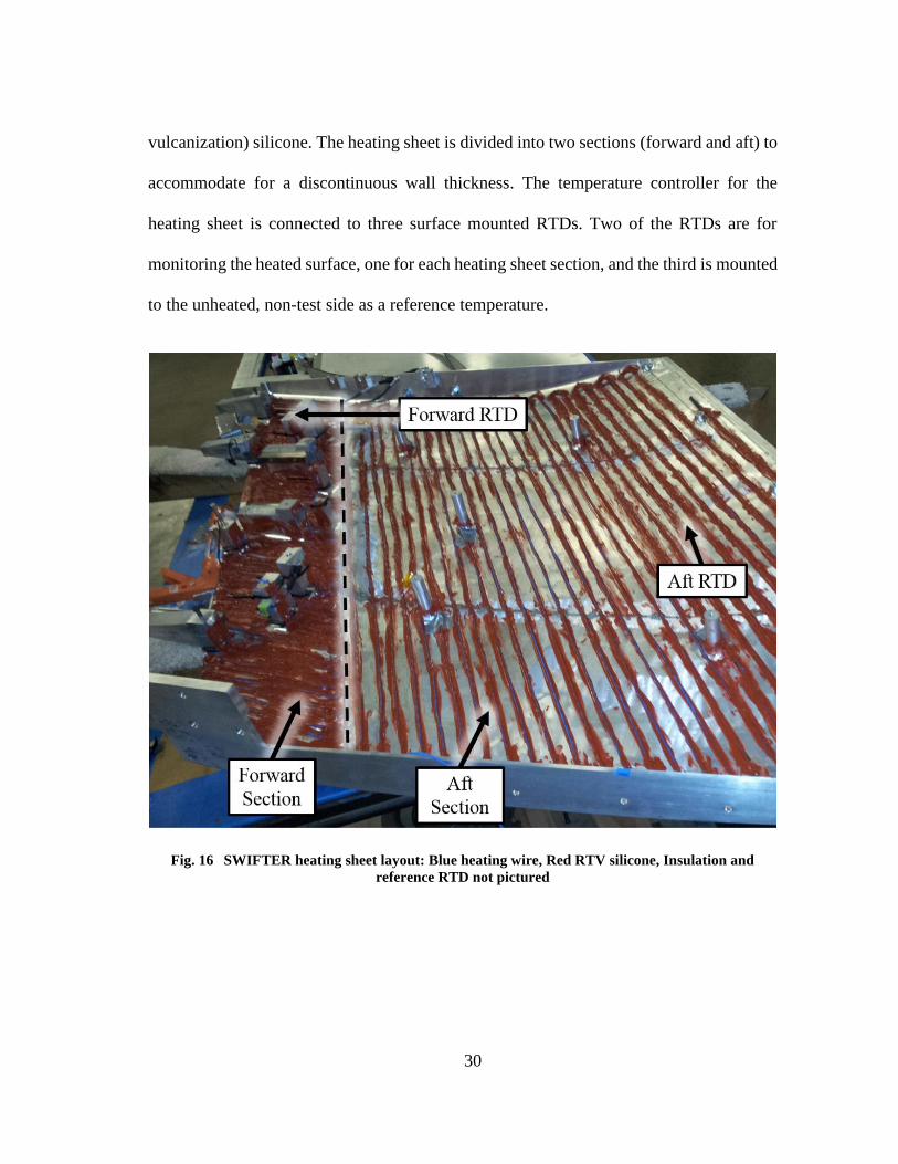
the surface temperature to a few degrees above the ambient Fig 16 depicts the internal

heating sheet constructed from pre-sheathed heating wire and RTV (room temperature

30

vulcanization) silicone The heating sheet is divided into two sections (forward and aft) to

accommodate for a discontinuous wall thickness The temperature controller for the

heating sheet is connected to three surface mounted RTDs Two of the RTDs are for

monitoring the heated surface one for each heating sheet section and the third is mounted

to the unheated non-test side as a reference temperature

Fig 16 SWIFTER heating sheet layout Blue heating wire Red RTV silicone Insulation and

reference RTD not pictured

31

This wall heating method precludes the need for a high altitude climb and cold soak

saving both time and fuel In this procedure the O-2A climbs to an altitude of 6500 ft

MSL needs only a few minutes to confirm uniform heating before rapidly descending for

the experimental dive An average of 8 experimental dives can be completed in

comparison to SWIFTrsquos 2 During the experimental dive the turbulent region is cooled

faster than the laminar region again this is due to the higher convection rate and shear

stress of the turbulent flow Fig 17 shows a graphical representation of this process In

this case the rapid descent is merely for achieving faster flow over the model and not

necessarily aimed at utilizing the increasingly warmer air while descending in altitude

Because the model is actively heated the surface is continuously a few degrees above the

ambient fluid flow however it is important to note that the temperature lapse rate can

overtake the heating sheetrsquos ability to maintain a higher surface temperature and was

experienced infrequently throughout the experimental campaign The maximum power

output of the heating sheet was approximately 500 W (Duncan 2014 [32])

32

Fig 17 Idealized graphic of wall heated model (not to scale) (top) Temperature distribution near

transition (bottom) (Crawford et al 2013 [35])

As mention earlier successful IR thermography of boundary-layer transition requires a

thin insulating layer on the surface that is capable of maintaining a strong temperature

gradient Additionally the surface must be as minimally-reflective in the IR wavelength

band as possible The SWIFT model was coated in a flat black powder coat that held a

strong gradient well however this powder coating was susceptible to reflections in the IR

band Features such as exhaust flare diffraction of light around the fuselage ground

terrain and reflections of the test aircraft could be seen on the model These reflections

33

could mask the transition process on the surface and contaminate the data The SWIFTER

model improved upon this drawback by utilizing Sherwin Williams F93 mil-spec aircraft

paint in lusterless black This coating provided the necessary insulation to achieve holding

a strong temperature gradient and also had low-reflectivity in the IR band While some

reflected features mainly exhaust flare could be observed the contamination was

miniscule These features are actually removed utilizing the IR image post-processing

code SWIFTERrsquos paint thickness was approximately 300 microm in comparison to SWIFTrsquos

100 microm the added thickness helps to sharpen any detail in the IR images

IR Camera Comparison

At the start of the SWIFT experimental campaign a FLIR SC3000 IR camera was used

for transition detection The SC3000 has a resolution of 320x240 pixels operates in the

8-9 microm wavelength band and can sample at a maximum frame rate of 60 Hz Toward the

end of the SWIFT campaign and for the entire SWIFTER campaign a new updated IR

camera was used the FLIR SC8100 The SC8100 has a resolution of 1024x1024 pixels

operates in the 3-5 microm wavelength band and can sample at a maximum frame rate of 132

Hz The SC8100 has a temperature resolution lower than 25 mK The SWIFT experiments

utilized a 17 mm lens while the SWIFTER flight experiments utilized a 50 mm lens

IR Image Processing

Throughout the entire SWIFT campaign and during the early stages of the SWIFTER

DRE campaign IR thermography was used as a qualitative transition detection tool

Transition location would be ascertained by human eye with an approximate uncertainty

of xc = plusmn005 These qualitative readings were very susceptible to human biasing error

34

and did not provide a consistent and accurate means of transition detection However this

was initially seen to be sufficient for DRE experiments because substantial transition delay

would be on the order of xc = 01 Currently quantifying the sensitivity of transition to

DREs requires a more accurate and robust method of transition detection Fig 18 and Fig

19 show an example of qualitative IR transition detection for the SWIFT and early

SWIFTER campaigns respectively these are raw IR images taken from the FLIR

ExaminIR software It is clearly obvious that there is a large uncertainty in picking out the

transition front In Fig 18 flow is from right to left and the laminar cooler region is

denoted by the orange color while the turbulent warmer region is denoted by the yellow

color This is indicative of the wall cooling process where turbulent flow relatively heats

the model surface In Fig 19 flow is diagonal from top-right to bottom-left and the

laminar warmer region is denoted by the lighter shading while the turbulent cooler

region is denoted by the darker shading This is indicative of the wall heating process

where turbulent flow relatively cools the model surface In Fig 19 more surface flow

detail is observed when utilizing the SC8100 and the 50 mm lens

35

Fig 18 Raw IR image from SWIFT model with qualitative transition front detection at 50 chord

(modified figure from Carpenter (2009) [14])

Fig 19 Raw IR image from SWIFTER model with qualitative transition front detection at 35-40

36

Even with the improved IR camera and images discerning the transition front was still

susceptible to human biasing error Brian Crawford (Crawford et al 2014a [36])

developed a solution for this problem by creating an IR post-processing code that removes

the human biasing error and inconsistency of qualifying transition location Additionally

this code is able to reliably and repeatably pull out a quantitative transition-front location

with an uncertainty on the order of xc = plusmn0001 This uncertainty does not include

systematic errors found in α and Reprime but merely accounts for variations in front detection

from frame to frame It is essentially negligible compared to the systematic uncertainty

Total uncertainty for transition-location detection is plusmn0025 xc on average Fig 20

compares a raw (left) and processed (right) IR image while quantifying a transition front

location at xc = 0487 plusmn 0001 Again this uncertainty value does not account for

systematic uncertainty The blue dashed lines in Fig 20 encompass the test area of the

model Additionally Fig 21 provides further perspective on the raw IR image orientation

by overlaying it onto an image of the SWIFTER model in flight

37

Fig 20 Comparison of raw (left) and processed (right) IR images

Fig 21 Raw IR image overlaid on SWIFTER model in flight

38

The post-processing code involves four major steps image filtering fiducialmodel

tracking image transformation and transition detection In order to remove any spatially

slow-varying features such as exhaust flare sunlight on the model or internal structure

illuminated by heating the IR image is spatially high-passed The image is then histogram

normalized so that contrast around temperatures with steep gradients are enhanced This

brings out a more defined transition front (aids in transition detection) and also makes the

crossflow streaking clearly visible Model tracking is accomplished by using three 508

mm square Mylar tape fiducials seen in Fig 20 The highly IR-reflective Mylar tape

provides a strong temperature gradient between the surface and itself by reflecting the

cooler ambient temperature allowing for easy detection Because the fiducials are placed

at known locations on the model surface the model orientation and position can now be

characterized in 3-D space relative to the camera Once model orientation and position are

known the raw IR image can then be transformed such that the chordwise direction is

horizontal and the spanwise direction is vertical with flow now from left to right (Fig 20

(right)) This transformation step essentially ldquoun-wrapsrdquo the surface of the model by

accounting for viewing perspective lens effects and model curvature Finally the

transition front is located by calculating the gradient vector at every pixel in the filtered

tracked and transformed image The resulting vector field is then projected onto the

characteristic direction along which turbulent wedges propagate The magnitude of these

projections determines the likelihood of each point being a location of transition larger

projections are most likely transition while smaller projections are least likely transition

This continues until the code converges on an overall transition front

39

Once the front is detected 20 consecutive processed images at the same experimental

condition are averaged together to obtain a single quantifiable transition front location

This is done by producing a probability density function (PDF) derived from a cumulative

distribution function (CDF) of the front for each of the 20 transition front locations The

abscissa (xc location) of the PDFrsquos maxima corresponds to the strongest transition front

Graphically it can be seen as the x-location of the largest peak in the PDF on the right

side of Fig 20 There are 20 colored lines representing each of the 20 analyzed images

that are centered around 1 second of being ldquoon conditionrdquo Being ldquoon conditionrdquo refers to

holding a target α and Reprime within tolerances for 3 seconds during the experiment Finally

the black curve is an accumulation of the 20 individual PDFs thereby quantifying the most

dominant transition location A key feature to using PDFs is that they are unaffected by

anomalies such as bug-strikes that would cast a single turbulent wedge That turbulent

wedge will receive a smaller PDF peak and not affect the more dominant larger peaks of

the front location Further detail on the IR post-processing code can be found in Crawford

et al (2014a) [36]

25 Traversing Laser Profilometer

Characterizing surface roughness is of key importance when conduction

laminar-turbulent boundary-layer transition experiments The surface roughness directly

affects the receptivity process by providing a nucleation site for the initial disturbances A

Mitutoyo SJ-400 Surface Roughness Tester was used for characterizing all SWIFT LE

configurations and for the polished LE of SWIFTER This device is a contact stylus

profilometer with maximum travel of 254 mm and a resolution 000125 microm when utilizing

40

the 80 microm vertical range setting While this device can locally characterize surface

roughness by means of the root-mean-square (RMS) and peak-to-peak (Pk-Pk) it is

incapable of measuring frequency content in the wavelength band that strongly influences

the crossflow instability (1-50 mm) To adequately resolve the power of a 50 mm

wavelength on a surface the travel of the profilometer must be able to acquire several

times that length in a single pass This need for surface roughness frequency analysis was

met by the design and fabrication of a large-span non-contact surface profilometer by

Brian Crawford (Crawford et al 2014b [37]) The traversing laser profilometer (TLP)

shown in Fig 22 utilizes a Keyence LK-H022 laser displacement sensor has a

chordwise-axis travel of 949 mm a LE-normal-axis travel of 120 mm surface-normal

resolution of 002 microm laser spot size of 25 microm and is capable of sampling at 10 kHz The

TLP was used to characterize the surface roughness of the painted SWIFTER LE and to

re-measure a previous SWIFT painted LE Those roughness results will be discussed in

the Surface Roughness section The reason the TLP was not used to characterize the

polished LE surface roughness was due to the noise generated by the laser reflecting off

of the highly-polished surface The noise floor was greater than the desired resolution to

characterize the frequency content

41

Fig 22 Traversing Laser Profilometer with labeled components (modified figure from Crawford et

al 2014b [37])

42

3 EXPERIMENTAL CONFIGURATION AND PROCEDURES

After completing improvements and upgrades to the model five-hole probe amp

calibration IR thermography image processing surface roughness analysis amp

measurement uncertainty a more accurate and discriminative DRE test campaign could

commence An overall experimental set-up is discussed along with a typical flight profile

and test procedures The surface roughness of the polished and painted leading edges is

characterized and discussed An introduction to linear stability theory is made and how it

relates to DRE configurations Finally DRE improvements specifications and

manufacturing processes are discussed along with which configurations were tested

31 Experimental Set-up Test Procedures and Flight Profile

Experimental Set-up

The SWIFTER model was mounted to the port outboard pylon of the Cessna O-2A

Skymaster with a 4deg yaw-angle-offset from the aircraft centerline szligoffset This is changed

from SWIFTrsquos szligoffset = 1deg in order to reduce the aircraft sideslip szlig required to achieve

desired model angles of attack α Moreover another structural change to SWIFTER from

SWIFT not mentioned earlier was the removal of a variable angle of attack mechanism

Because the SWIFT szligoffset was never changed the added complexity was deemed

unnecessary Fig 23 is a schematic detailing the model offset from the O-2A and similarly

offset from the freestream velocity vector

43

Fig 23 SWIFTER and SWIFT szligoffset schematic (angles are exaggerated for visualization purposes)

(modified figure from Duncan (2014) [32])

As mentioned earlier the 5HP is attached to the non-test side of SWIFTER and

coupled with a static-temperature sensor measures freestream conditions and the attitude

of the model The FLIR SC8100 IR camera is used for globally capturing

laminar-turbulent transition Electrical power is supplied to the entire instrumentation

suite through an 1100 W power inverter Fig 24 shows the instrumentation layout of the

O-2A rear cabin The SC8100 is aimed through a window cutout because the plexiglass

in the O-2A is not IR-transparent If there was no cutout the camera would simply detect

44

the temperature of the plexiglass An in-house-built LabVIEW virtual instrument (VI)

running on a laptop controls all aspects of information display data acquisition and model

control The flight crew consists of five persons three of which are in the aircraft during

operations Positions include a test pilot co-pilotsafety observer flight test engineer

(FTE) and two ground crew operators

Fig 24 Instrumentation layout in rear of O-2A cabin (Duncan 2014 [32])

Test Procedures and Flight Profile

For safety reasons flight operations at the TAMU-FRL are restricted to daylight VFR

(visual flight rules) conditions Because of this daylight restriction ideal flight conditions

including no cloud cover low atmospheric turbulence linear temperature-altitude lapse

rate and low temperature all tend to align in the early hours of the day (ie sunrise to

DAQ boards

FTE seat

IR camera

CO monitor

Power inverter

Window cutout

for SWIFTER

view

SWIFTER

control box

Pressure

transducer box

Window for

hotwire sting

mount view

45

approximately 0900 local) Past 0900 the Sun increases the temperature of the surface

which causes updrafts resulting in increased turbulence Additionally increased

temperature negatively affects the maximum attainable unit Reynolds number

Consideration of all these variables causes every DRE flight experiment to begin the day

prior to the actual flight DRE array applications take approximately 2 hours to complete

The application process will be discussed in a later section Itrsquos important to note that

during the SWIFTER excrescence campaign it was discovered empirically that the

moveable LE while secured with linear actuators and an electromagnet drifts

approximately 30 microm toward the non-test side during the experimental dive due to

aerodynamic loads on the LE If the step at 15 chord was zeroed before the flight then

during the experiment there would exist a 30 microm forward facing step at that location

Because of this drift under loading the LE is set to a 30 microm aft facing step on the ground

before the flight This step is checked with feeler gauges before and after each flight and

is adjusted if necessary

After the DRE array has been applied and all instrumentation and safety checklists have

been completed by the flight crew the aircraft is ready to takeoff and depart toward the

test area Because the SWIFTER heating sheet draws a significant amount of power it is

not turned on until immediately after takeoff While the model is being internally heated

the aircraft is climbing to a test altitude ranging from 6500 to 7500 ft MSL Once the

aircraft reaches the test altitude the surface of the model has been uniformly heated to a

few degrees above the ambient temperature At this point a set of pre-dive checklists are

performed in order to ensure the correct test conditions are set in the pilotrsquos yoke display

46

and that all instrumentation is functioning properly and acquiring data During the

experimental dive the test pilot holds the model at a constant α while increasing Reprime in

010 x 106m increments this procedure is called a ldquoReynolds sweeprdquo Crew duties during

the dive are as follows

FTE Test conductor ndash informs pilot of test conditions and procedures

Test Pilot Controls the aircraft in order to maintain constant conditions

Co-PilotSafety Observer Continuously scanning outside the aircraft for traffic

and clouds (This position is essential because the test pilot is focused on

instruments and displays during the experimental dive)

Because of where natural transition occurs on SWIFTER with either the polished or

painted LE installed the model is flown at unit Reynolds numbers ranging from 48 - 60

x 106m and at two different angles of attack -65deg amp -75deg These conditions correspond

to speeds in the range of 150-175 KIAS and a szlig of 25deg amp 35deg For safety reasons the

experimental dive is completed once the aircraft has descended to approximately 3000 ft

MSL The climb and dive procedure is repeated until there is not enough fuel remaining

to complete another dive at which point the aircraft returns to Easterwood Airport Fig

25 shows a typical flight profile for conducting the experiment while Fig 26 shows a

typical Reprime and α trace while holding conditions for 3 seconds

47

Fig 25 Typical flight profile

Fig 26 Typical Reprime and α traces while on condtion

48

32 Surface Roughness

It became obvious early in the swept-wing research program circa 1990 that micron-

sized roughness in millimeter-sized boundary layers played a very strong role in

influencing transition on a swept wing eg Radeztsky et al (1999) [38] In the Carpenter

et al (2010) [28] SWIFT experiments the baseline roughness for the polished LE was

033 microm RMS and 22 microm average peak-to-peak Transition occurred at 80 chord for

this polished leading edge therefore this was not a useful baseline for evaluating DREs

To move transition forward the leading edge was painted and sanded with very little

attention paid to uniformity and overall quality Several local measurements using the

Mitutoyo SJ-400 taken at 1 chord along the span in 25 mm increments gave a roughness

of 17 microm RMS and 77 microm average peak-to-peak Itrsquos important to note the discontinuous

change in surface roughness on the painted leading edge Only the first 2 chord of the

model was sanded using 1000-grit sandpaper resulting in the previously stated RMS and

average peak-to-peak The remaining leading edge region from 2 to 15 was untouched

after painting and had a roughness of 624 microm RMS and 3142 microm average peak-to-peak

(Carpenter 2009 [14]) Because of the increased roughness transition moved to 30

chord at a unit Reynolds number of Re = 550 x 106m It was with this configuration that

any laminarization was achieved with DREs The paint was eventually removed without

further documentation

As part of a cooperative program with NASA-DFRC on a LFC experiment with a

Gulfstream G-III aircraft TAMU-FRL was asked to re-examine the Carpenter et al

(2010) [28] experiments so the leading edge was repainted With this new paint finish the

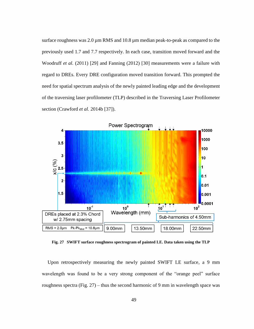
49

surface roughness was 20 microm RMS and 108 microm median peak-to-peak as compared to the

previously used 17 and 77 respectively In each case transition moved forward and the

Woodruff et al (2011) [29] and Fanning (2012) [30] measurements were a failure with

regard to DREs Every DRE configuration moved transition forward This prompted the

need for spatial spectrum analysis of the newly painted leading edge and the development

of the traversing laser profilometer (TLP) described in the Traversing Laser Profilometer

section (Crawford et al 2014b [37])

Fig 27 SWIFT surface roughness spectrogram of painted LE Data taken using the TLP

Upon retrospectively measuring the newly painted SWIFT LE surface a 9 mm

wavelength was found to be a very strong component of the ldquoorange peelrdquo surface

roughness spectra (Fig 27) ndash thus the second harmonic of 9 mm in wavelength space was

50

at the most unstable wavelength (45 mm) and was strongly excited The strong excitation

of the most unstable wave prevented any observations of laminarization due to DREs The

most unstable wave will be discussed further in the following Linear Stability Theory

section

Similar to the SWIFT experiments two separate leading edge (LE) surface-roughness

configurations were used during the SWIFTER DRE experimental flight campaign as

shown in Fig 28 The two interchangeable LE surface configurations consisted of a highly

polished aluminum surface characterized by an RMS of 02 microm amp median peak-to-peak

of 12 microm and a painted surface characterized by an RMS of 13 microm amp median peak-to-

peak of 70 microm The polished surface finish was obtained through progressive wet-sanding

using 400 through 3600 grit sand paper followed by a series of four increasingly finer-

graded metal polishes The painted surface finish was obtained by first sealing sanding

and painting a pressure-tapped aluminum LE with JetGlo aircraft paint followed by

progressive wet-sanding using 600 through 1200 grit sand paper in order to remove any

ldquoorange peelrdquo type frequency excitation

Fig 28 SWIFTER model in flight with polished (left) and painted (right) LE installed

51

Surface Roughness Measurement Procedure

As discussed earlier local roughness measurements were taken on the polished LE

using the Mitutoyo SJ-400 in order to characterize the RSM and Pk-Pk The traversing

laser profilometer was used to characterize RMS Pk-Pk and frequency content of the

painted LE Frequency content was not analyzed on the polished LE because of laser

reflection and sensor noise Fig 29 shows the experimental setup of the TLP and the

SWIFTER LE

Fig 29 SWIFTER LE being measured with the TLP

In order to characterize the entire LE from -0004 to 0150 xc the LE must be placed

at three separate positions (a b amp c of Fig 30) due to the 120 mm travel limitation in the

52

LE-normal direction Negative xc positions refer to the non-test side of the SWIFTER

model A wooden LE stand was constructed in order to repeatably measure different

section of the LE The measurement ranges for the three positions in Fig 30 are as follows

a) xc = 0005 ndash 0077 b) xc = -0004 ndash 0005 and c) xc = 0067 ndash 0150

Fig 30 Wooden LE stand for traversing laser profilometer measurements

The following three figures Fig 31 Fig 32 and Fig 33 show the frequency content

of the painted LE in a spectrogram format for the LE stand positions of b) a) and c)

respectively The paint application is relatively broadband with no strong critical

53

wavelengths that would negatively affect the crossflow instability The 35 mm spike seen

in all three images is inherent to the TLP It is most likely caused by some ball passing

frequency of the bearings in the chordwise-axis linear actuator Additionally no sub-

harmonics of the most unstable wavelength (450 mm) exist as previously seen in the

SWIFT painted surface spectra

Fig 31 SWIFTER painted LE spectra for xc = -0004 ndash 0004 (-04 to 04 chord)

54

Fig 32 SWIFTER painted LE spectra for xc = 0005 ndash 0077 (05 to 77 chord)

Fig 33 SWIFTER painted LE spectra for xc = 0067 ndash 0146 (67 to 150 chord)

55

33 Linear Stability Theory

Modeling disturbance growth by using three-dimensional Navier-Stokes equations is

often computationally expensive and is initial-condition dependent Linear Stability

Theory and the eN method are typically viewed as simplified transition prediction schemes

for determining disturbance amplification associated with a particular instability and its

transition location The basic concept behind LST is to superpose small disturbances onto

the local undisturbed boundary-layer state (basic state) and determine whether these

perturbations grow or decay (Reed et al (1996) [39]) Some assumptions inherent to LST

include small disturbances parallel flow unsteady and linearized Navier-Stokes This

section will focus on the applicability of LST to controlling the crossflow instability with

DREs

In this experiment Linear Stability Theory is used strictly to identify the most unstable

wavelength and branch I neutral point (where this most unstable wavelength begins to

grow) Additionally the eN method uses the growth rates from LST to ldquopredictrdquo that

transition will occur after a certain amplification ratio has been met This amplification

ratio referred to as the N-Factor is shown in Eq 1

119873 = int minus120572119894 = ln119860

1198600

119909

1199090 (1)

In Eq 1 A0 is the initial disturbance amplitude and A is the disturbance amplitude at

the x-location downstream Because the initial disturbance amplitude A0 is not typically

known this amplification factor can only predict relative disturbance growth and decay

Fig 34 shows the relationship between N-factor and chord for multiple wavelengths of

56

the SWIFTER model at α = -65deg and Reprime = 550 x 106m From the plot on the left in Fig

34 the most unstable wavelength was determined to be 450 mm (largest N-Factor and

growth rate) with a candidate control wavelength of 225 mm Candidate control

wavelengths are typically 50-60 of the most unstable wavelength Additionally the

branch I neutral point for the most unstable wavelength on the SWIFTER model is located

at xc = 0023 while the branch I neutral point for the candidate control wavelength is

located at xc = 0009 (seen in the right-hand-side plot in Fig 34) Previous experiments

have shown success by placing the DRE arrays spaced at the control wavelength at the

branch I neutral point of the most unstable wavelength The computational support for this

research was conducted by Matthew Tufts a PhD candidate at Texas AampM University

Fig 34 N-Factor plot for SWIFTER at α = -65deg and Reprime = 55 x 106m The plot on the right is a

zoomed in version of the plot on the left

It is generally accepted that N-Factors ranging from 9 to 14 ultimately result in

transition while control N-Factors range from 5 to 8 however these numbers are largely

57

determined experimentally A maximum N-Factor Nmax is achieved by placing the DRE

array at the branch I neutral point of its respective wavelength For example placing an

array of DREs spaced at 225 mm at an xc of 0009 results in a maximum N-Factor of 82

An effective N-Factor Neff is achieved by placing the DRE array downstream of the

branch I neutral point of its respective wavelength For example placing an array of DREs

spaced at 225 mm at an xc of 003 results in an effective N-Factor of 67 Table 3 outlines

the specific maximum and effective N-Factors for this experiment at α = -65deg and Reprime =

55 x 106m It is evident that the Neff decreases as you reduce the wavelength or increase

the xc location The location of the branch I neutral points do not vary significantly with

α and Reprime but the N-Factors do vary and should always be accounted for

Table 3 Effective N-Factor Chart for SWIFTER at α = -65deg amp Reprime = 55 x 106m

Avg xtrbaseline = 046

Ntr = 119 Chord Location (xc)100

110 220 300 325 350

DR

E W

av

elen

gth

(λ

) 275 mm (Nmax = 104) 104 100 94 93 91

250 mm (Nmax = 93)

93 87 81 79 77

225 mm (Nmax = 82) 81 73 67 65 63

200 mm (Nmax = 70) 70 60 53 50 49

34 Spanwise-Periodic Discrete Roughness Elements

The DREs were manufactured by Pixels 2 Press (P2P) a print media service company

located in Norwalk Connecticut P2P has been able to consistently provide superior dry-

transfer DREs at an average height of 12 microm Previously the company Redd Europe was

58

the main DRE supplier however P2P has been able to produce higher quality DREs at a

lower price and can ship their orders in a matter of days rather than weeks as with Redd

Europe Based on LST the DREs utilized should range in wavelength from 2 ndash 3 mm in

increments of 025 mm As different DRE configurations are discussed in later sections a

particular nomenclature will be used to succinctly describe each configuration For

example [12microm|225mm|1mm|23|02-14] describes a DRE array that is 12 microm tall has

a wavelength (center to center) of 225 mm a diameter of 1 mm placed at 23 chord on

the SWIFTER model and orderedprinted during the month of February 2014 Fig 35

shows a 3-D scan of P2P DREs using a Keyence VK-9710 confocal laser microscope

59

Fig 35 3-D scan of Pixels 2 Press DREs spaced at 225 mm

Application Technique

The technique for applying DREs to the LE involved chord markers on the top and

bottom surface of the LE seen in Fig 36 (left) and the use of a monofilament (fishing

line) aligned to the chord markers Because the DREs are 1 mm in diameter the

monofilament was place 05 mm aft of the intended DRE chord location so as to align the

centers of the DREs with the desired location seen in Fig 36 (right) The DRE array did

not span the entire model but would extend above and below the root and tip pressure

60

port rows so as to not cast a turbulent wedge in the test area of the model The uncertainty

of DRE array placement on the model is plusmn007 chord which equates to plusmn1mm along the

chord line

Fig 36 DRE application photos constant chord markers (left) DRE amp monofilament alignment

(right)

Laminar flow control using DREs

The basic idea behind using DREs for LFC is to delay the growth of the crossflow

instability by forcing a single mode thereby precluding or delaying the growth of the most

unstable mode DREs are applied at wavelengths less than the most amplified wave (450

mm) in an attempt to suppress or delay growth of the linearly most unstable wavelength

As seen in Saric et al (1998a 1998b) [16 17] harmonics and never sub-harmonics in

wavenumber space appeared for a given roughness condition Additionally the control

wavelength will decay before amplitudes large enough to cause transition can be reached

thereby delaying transition or extending laminar flow Placement of control DREs at the

61

branch I neutral point is intended to delay the growth of the most unstable wavelength at

its source In this experiment several chord locations are tested The effect of placing

DREs after the branch I is not completely understood as the most unstable wavelength

has started to grow and then mixes with the forced wavelength of the DREs Further

computational studies could expand upon this interaction To restate the method of control

applying DREs having a wavelength less than the most amplified wave is intended to

suppress the linearly most unstable wavelength and only admits the induced roughness

wavelength and its harmonics in wavenumber space For example forcing a 900 mm

wavelength would admit its harmonics of 450 mm and 225 mm etc to grow while

prohibiting the growth of any sub-harmonics such as 1800 mm or 36 mm This forcing

would obviously be counterproductive to control because the most unstable wavelength is

allowed to grow Conversely forcing a sub-critical 225 mm wavelength would admit its

harmonics and not its sub-harmonics which include the most unstable 450 mm

wavelength Control wavelengths are generally 50-60 of the most unstable wave (Saric

et al 2004 [3]) Table 4 and Table 5 enumerate the DRE configurations tested throughout

the experiment for the polished and painted leading edges respectively

62

Table 4 DRE configurations tested on the polished LE

DRE Array Nomenclature

[Height (k) in microm | Wavelength (λ) | Diameter (d) in mm | Chord Location | Batch Date (MM-YY)]

Denotes flights before IR post-processing was possible

Polished LE Configurations

Date Stamp O-2A Flight Configuration

041913-1 792 [11microm|275mm|1mm|22|08-12]

041913-2 793 [22microm|275mm|1mm|22|08-12]

042013-1 794 [11microm|225mm|1mm|22|05-12]

062913-1 801 [11microm|225mm|1mm|30|05-12]

063013-1 802 [11microm|225mm|1mm|30|05-12]

070313-1 806 [11microm|250mm|1mm|30|08-12]

091213-1 824 [11microm|225mm|1mm|30|05-12]

091813-1 828 [12microm|200mm|1mm|30|07-13]

092413-1 829 [11microm|225mm|1mm|35|05-12]

122313-1 836 [12microm|225mm|1mm|35|11-13]

021514-1 840 [12microm|225mm|1mm|35|11-13]

022114-1 842 [12microm|275mm|1mm|35|11-13]

022214-1 843 [12microm|225mm|1mm|325|11-13]

022714-2 845 [12microm|225mm|1mm|35|11-13]

031314-1 847 [12microm|225mm|1mm|30|02-14]

031714-1 848 [12microm|250mm|1mm|35|02-14]

031814-1 850 [12microm|225mm|1mm|325|02-14]

032514-1 851 [12microm|225mm|1mm|325|02-14]

033014-1 853 [12microm|250mm|1mm|30|02-14]

041514-1 858 [12microm|200mm|1mm|20|02-14]

63

Table 5 DRE configurations tested on the painted LE

DRE Array Nomenclature

[Height (k) in microm | Wavelength (λ) | Diameter (d) in mm | Chord Location | Batch Date (MM-YY)]

Painted LE Configurations

Date Stamp O-2A Flight Configuration

050514-1 863 [12microm|225mm|1mm|23|02-14]

051514-1 864 [12microm|225mm|1mm|35|02-14]

051614-1 865 [12microm|225mm|1mm|35|02-14]

062114-1 870 [12microm|225mm|1mm|35|11-13]

062314-1 871 [12microm|225mm|1mm|11|11-13]

64

4 RESULTS

In total 63 SWIFTER-DRE flights have been completed while only 30 of those flights

resulted in useable data Of those 30 flights 5 where baseline flights (4 polished amp 1

painted) Of the 25 DRE flights 3 were completed before the IR fiducials were added

leaving ΔLF analysis for the remaining 22 Reasons for un-useable data include bug

strikes damaged DRE arrays excessive atmospheric turbulence and instrumentation

failure While the post-processing code is insensitive to bug strikes when locating

transition the location of the bug strike can obscure the entire front if impact was at or

near mid-span Before commenting on any specific results it is important to briefly re-

state the major uncertainties in the experiment Total uncertainty in α typically ranges from

012ordm to 014deg but can be as low as the systematic uncertainty (010deg) Unit Reynolds

number (Reacute) total uncertainty typically ranges from 002 - 003 x 106m but can be as

low as the systematic uncertainty (0015 x 106m) Leading edge sweep total uncertainty

typically ranges from 023-025deg but can be as low as the systematic uncertainty (022deg)

Transition location total uncertainty typically ranges from 25 - 27 chord which results

in a percent-laminar-flow increase or decrease total uncertainty that ranges from 10 - 15

depending on where transition is located on the model It is important to note that nothing

significant can be said about a percent-laminar-flow increase or decrease below 10

Again an extensive uncertainty analysis can be found in Duncan (2014) [32]

In this chapter the IR thermography results will be discussed and quantified into a new

variable that denotes change in percent-laminar-flow ΔLF Baseline curve fits of

65

transition data and the unexpected laminarization of increased surface roughness will be

discussed Finally an overview of these results will be provided

41 Infrared Thermography Transition Data

First a brief description of the post-processed IR image is necessary to understand how

best to interpret the data contained in it Fig 37 is an example of a post-processed IR

image At the top of the figure the date timestamp α and Reprime are displayed for each

image with their respective uncertainty The nominal conditions for this test point were α

= -75deg and Reprime = 530 x 106m With flow from left to right the transition front is the

quintessential saw-tooth pattern seen in stationary-crossflow transition Additionally

crossflow streaking before the transition front can be seen clearly The darker blue-green

region is laminar flow while the lighter pink-green region is turbulent flow The x-axis

shows lines of constant chord (xc) while the z-axis shows lines of constant span The

black specks at the top of the colored image are the tip pressure ports There are two large

half-wedges that can be seen at the top and bottom of the colored image these wedges are

propagating from pieces of Velcro that were adhered to the model in order to create

constant turbulent flow over the pressure ports This also helps clearly define the test area

and give a reference for turbulent flow Finally the colored curves above the IR image are

the 20 PDF lines that cumulate to a single black PDF curve whose maxima defines the

transition front location Total transition front uncertainty ranges from 0025 ndash 0027 xc

(25 - 27 chord)

66

Fig 37 Example post-processed IR image

At the beginning of the experiment the process to determine an increase or decrease in

laminar flow was to look at two post-processed IR images (baseline flight and DRE flight)

67

and simply take the difference between their transition locations This was initially

considered adequate to determine changes in laminar flow because both test points

(baseline and DRE) were held at the same target α and Reprime for 3 seconds within a given

tolerance The tolerance of the ldquoon conditionrdquo mean value is plusmn005deg for α and plusmn005 x

106m for Reprime Fig 38 shows an example of direct IR comparison between a baseline and

DRE flight with target conditions of α = -65deg and Reprime = 570 x 106m It is first obvious

that the transition front has moved forward thereby decreasing the amount of laminar flow

by 46 (ΔLF = -46) ΔLF is calculated using Eq 1 where a positive number

represents more laminar flow and a negative number represents a loss of laminar flow

The nominal α and Reprime are input in the baseline transition equations found in the next

section in order to determine the nominal baseline transition location

∆119871119865 = (119909119905119903119887119886119904119890119897119894119899119890minus119909119905119903119863119877119864

119909119905119903119887119886119904119890119897119894119899119890) times 100 (1)

However notice that the difference in Reprime between the two conditions is 008 x 106m

While both Reprime values are within the allowed tolerance their spread is almost an entire test

point away Recall that the Reynolds sweep changes in increments of 01 x 106m

therefore making the comparison between these points almost invalid Problems arose in

the middle of the experiment campaign due this lack of care when comparing fronts For

example a few configurations showed promise with a ΔLF of 20 however once the

differences between α and Reprime were accounted for the ΔLF dropped back below the

uncertainty of the calculation (plusmn10) While the direct comparison method is acceptable

for α whose total uncertainty is plusmn013deg it is not for Reprime whose total uncertainty is plusmn002

x 106m (lower than the tolerance of ldquoon conditionrdquo) The only way to accurately compare

68

between two points is to account for the differences in both α and Reprime This is accomplished

by creating a baseline transition curve fit that is dependent on both α and Reprime

Fig 38 Direct IR comparison between baseline flight 862 (left) and DRE flight 863 (right) with

target conditions of α = -65deg amp Reprime = 570 x 106m [12microm|225mm|1mm|230|02-14]

42 Baseline Curve Fit

The baseline curve fits for the polished LE is comprised of 4 separate baseline flights

while the baseline curve fit for the painted LE is comprised of a single flight Fig 39 and

Fig 40 graphically show the polished and painted fits along with their respective

governing equation and RMSE Duncan (2014) [32] calculates a similar fit utilizing the

same technique freestream conditions and model AoA range Those data are actually

69

included in the polished baseline curve fit and account for one of the four flights that

comprise the data set

Fig 39 Baseline-transition surface fit for polished leading edge

xtrpolished-baseline c = 3954 + (015α) + (-45e-7Reprime)

70

Fig 40 Baseline-transition surface fit for painted leading edge

xtrpainted-baseline c = 3439 + (014α) + (-36e-7Reprime)

Surface Roughness Conundrum

As mentioned earlier increased surface roughness has historically moved transition

forward thereby reducing the amount of laminar flow over a wing (Carpenter et al (2010)

[28] Carpenter (2009) [14] Radeztsky et al (1999) [38]) When viewed from the

perspective of receptivity the larger surface roughness directly introduces larger

disturbance amplitudes which allows for more available paths to breakdown then

turbulence As stated earlier in the Surface Roughness section the polished LE is

characterized by an RMS of 02 microm and a Pk-Pk of 12 microm while the painted LE is

characterized by an RMS of 13 microm and a Pk-Pk of 70 microm In opposition to countless

experiments and general theory the transition front of the painted LE was unexpectedly

aft of the polished configuration Additionally the main reason for increasing the surface

71

roughness of the SWIFTER LE was to reduce the amount of laminar flow by bringing the

transition location forward in chord This theoretical forward transition location would

have allowed for both an increase in model AoA during the experiment and would more

realistically simulate a production aircraft surface finish Fig 41 compares the polished

and painted transition locations as a function of unit Reynolds number and at a constant

AoA of -65deg Fig 42 compares the same for a -75deg AoA Additionally the baseline curve

fits for the same constant AoA is superimposed for each LE configuration

Fig 41 Baseline transition comparison for α = -65deg

72

Fig 42 Baseline transition comparison for α = -75deg

These are rather astounding results that cannot be explained at this time However there

is one potential theory that is offered to try and conjecture at the potential causes of this

behavior The idea is that small isolated 3-D imperfections in the LE whether caused by

local corrosionpitting of the aluminum or particle impact during flight create localized

disturbances that propagate into isolated turbulent wedges The periodicity of these

isolated wedges is larger than natural transition thereby masking the actual more uniform

front Regardless of origin or source this unexpected result should not hinder the

evaluation of DREs as a LFC technique

73

43 Percent-Change in Laminar Flow Data

When testing DRE configurations located at the branch I neutral point of the target and

control wavelengths for the polished and painted LEs no increase in laminar flow was

observed The configurations include

bull [11microm|225mm|1mm|11|05-12]

bull [11microm|275mm|1mm|23|08-12]

bull [22microm|275mm|1mm|23|08-12]

bull [11microm|225mm|1mm|23|05-12]

bull [12microm|225mm|1mm|23|02-14]

bull [12microm|225mm|1mm|11|11-13]

As a representative analysis more detail will be shown for the painted LE DRE

configuration [12microm|225mm|1mm|11|11-13] flown on 23 June 2014 Fig 43 and Fig

44 graphically show transition location as a function of unit Reynolds number for an AoA

of -65deg and -75deg respectively Both the associated baseline flight and DRE flight data

points are shown Also included on the chart is a reference to the baseline-transition

surface fit for the respective AoA and the percent-change in laminar flow ΔLF Again

ΔLF quantifies the amount of laminar flow gained or lost between the DRE transition

location and its baseline surface fit The percent-change in laminar flow scale can be found

on the second y-axis on the right side of the plot The dashed lines represent the uncertainty

for the baseline curve fit and ΔLF Uncertainty in ΔLF varies widely depending on

where transition is occurring Generally the uncertainty is higher at larger Reprime where

transition is farther forward and is caused by the lower overall amount of laminar flow It

74

is clearly evident that a significant loss in laminar flow is observed Fig 45 and Fig 46

are IR image comparisons from the same flight for the following test points respectively

bull AoA = -65deg amp Reprime = 550 x 106m ΔLF asymp -60

bull AoA = -75deg amp Reprime = 530 x 106m ΔLF asymp -55

In Fig 45 and Fig 46 the baseline test point is on the left while the DRE test point is on

the right

Fig 43 DRE flight 871 transition comparison for α = -65deg

75

Fig 44 DRE flight 871 transition comparison for α = -75deg

76

Fig 45 Direct IR comparison between baseline flight 862 (left) and DRE flight 871 (right) with

target conditions of α = -65deg amp Reprime = 550 x 106m [12microm|225mm|1mm|110|11-13]

77

Fig 46 Direct IR comparison between baseline flight 862 (left) and DRE flight 871 (right) with

target conditions of α = -75deg amp Reprime = 530 x 106m [12microm|225mm|1mm|110|11-13]

Results from this point on will be presented in a format identical Fig 43 and Fig 44

where the baseline curve fits are used to quantitatively determine the increases and

decreases in percent laminar flow For reference all post-processed IR images for each

ldquoon-conditionrdquo test point are included in a separate file This file is broken down into each

successfully completed baseline and DRE flight

While the decrease in laminar flow was extremely significant in the last example a

more typical ΔLF is generally in the -30 to 10 percent range The next two flights are

more representative of the majority of DRE configurations flown The configuration

[12microm|225mm|1mm|30|02-14] flown on 13 Mar 2014 essentially had no change in

transition front location This is shown graphically in Fig 47 and Fig 48 The

78

configuration [12microm|225mm|1mm|35|11-13] flown on 21 Jun 2014 experienced a 10-

20 loss in laminar flow This is shown graphically in Fig 49 and Fig 50

Fig 47 DRE flight 847 transition comparison for α = -65deg

79

Fig 48 DRE flight 847 transition comparison for α = -75deg

Fig 49 DRE flight 870 transition comparison for α = -65deg

80

Fig 50 DRE flight 870 transition comparison for α = -75deg

Finally one of the more interesting results was the configuration

[11microm|225mm|1mm|35|05 12] flown on 24 Sep 2013 This particular flight resulted

in a 10-50 increase in laminar flow These results are shown graphically in Fig 51 and

Fig 52 At first this seemed to be the exact configuration needed to extend laminar flow

for the SWIFTER model with a polished LE installed however upon several attempts at

repeating the configuration no duplication of the laminar flow increase was ever achieved

Fig 53 and Fig 54 show attempts at repeating this configuration with no success at

laminarization There were six separate attempts at reproducing the laminar flow increase

for repeatability Presently there is still more investigation into this flight to determine

why the results were so atypical however at this stage the flight must be considered an

anomaly

81

Fig 51 DRE flight 829 transition comparison for α = -65deg

Fig 52 DRE flight 829 transition comparison for α = -75deg

82

Fig 53 DRE flight 840 transition comparison for α = -75deg

Fig 54 DRE flight 865 transition comparison for α = -75deg

83

In summary out of the 30 flights with useable data only one showed a significant

increase in laminar flow while the rest either showed no change or a decrease in laminar

flow Also there was no apparent correlative trend between transition location and DRE

configuration other than the fronts moving significantly forward as the DREs where placed

closer to the attachment line One parameter not investigated was the effect of DRE height

on transition location mainly due to the manufacturing process of the DREs It is readily

agreed upon that the closer you move to the attachment line the shorter your DREs need

to be Appendix A is a compilation of the percent-change in laminar flow figures from

each flight ΔLF figures for flights 792 793 amp 794 are not included in the list because

the capability to post-process the IR images was not available due to the lack of surface

fiducials at that point in the experiment

84

5 SUMMARY CONCLUSIONS AND RECOMMENDATIONS

The aim of this research was to both reproduce the delay of laminar-turbulent transition

in flight using DREs and to determine the sensitivity of transition to variations in DRE

configuration Transition data was gathered using IR thermography while the SWIFTER

model was flown at AoAs of -65deg amp -75deg and unit Reynolds numbers ranging from 48 ndash

60 x 106m After several significant improvements were made to the previous

TAMU-FRL DRE flight experiments 63 DRE flights utilizing the new SWIFTER model

were completed with 30 of those flights returning useable data Of those 30 flights only

one showed a significant increase in laminar flow while the rest either showed no change

or a reduction in laminar flow

51 Flight-Test Summary

Initially the practice for determining an increase or decrease in laminar flow was to

directly compare processed IR images (DRE to baseline) taken at nominally the same

flight conditions More specifically small changes in AoA where essentially ignored and

small changes in Reprime where only qualitatively accounted for In actuality a change in Reprime

of 005 x 106m at constant AoA will change the transition front location by

approximately 2 and a change in AoA of 01deg at constant Reprime will change the transition

front location also by approximately 2 This direct image comparison technique has been

the practice for all previous TAMU-FRL DRE flight experiments and greatly limits results

of the experiment While using this direct comparison technique several instances of

increased laminar flow were observed mainly at two specific AoA and Reprime combinations

85

(AoA = -65deg Reprime = 55 x 106m) and (AoA = -75deg Reprime = 53 x 106m) where the max

increase in laminar flow observed was approximately 20 However with the

implementation of the baseline curve fit technique where small changes in AoA and Reprime

were now accounted for the number of instances of increased laminar flow dropped quite

significantly The remaining occurrences fell within the uncertainty of transition location

detection with the exception of flight 829

Upon achieving significant laminar flow extension as in flight 829 several flights

aimed at repeatability were unsuccessful and a parametric study ensued in order to detune

the best configuration for control No apparent correlative trend between transition

location and DRE configuration was observed other than the fronts moving significantly

forward as the DREs where placed closer to the attachment line Generally DREs placed

at 23 chord or forward would significantly move the front forward Itrsquos important to

note that one parameter not investigated in this experiment was the effect of DRE height

on transition location mainly due to the manufacturing process of the DREs The results

of this research have not confirmed the use of DREs as viable laminar flow control

technique in the flight environment Appendix A compiles the ΔLF plots for the

successful DRE flights and Appendix B compiles the post-processed IR images for the

successful DRE and baseline flights

52 Future Research Recommendations

Without repeatable consistent and correlated results relating DRE configuration to

transition front location it is not recommend that further DRE flight tests be conducted

until more information has been gathered with the possible exception of resurrecting the

86

F-15B experiments (Saric et al 2004 [3]) In the F-15B experiments T-S waves were the

dominant subsonic transition instability at the following flight conditions (M = 0911 Reprime

= 81 x 106m) Critically spaced DREs (4 mm for this particular airfoil shape) were

applied near the leading edge in order to force the most unstable wavelength to grow and

thereby move the transition front forward reducing laminar flow However the unique

result of this test was that full-chord laminarization was achieved when the baseline

transition location was already at 70 chord It is believed that the growth of the stationary

crossflow waves modified the mean flow thereby restricting the growth of the T-S wave

Additionally it is thought that the DREs can favorably influence traveling T-S waves by

making the base state spanwise periodic Further investigation into this phenomenon

would be beneficial to T-S dominated high-altitude surveillance aircraft

The main recommendation of this research effort is to further investigate DREs

computationally With the plethora of data collected during this flight campaign

computational studies specifically direct numerical simulation (DNS) of these particular

DRE configurations and flight conditions are a necessity in order to better understand the

influence that DREs have on laminar-turbulent transition A focus should be placed on

this experimentrsquos DRE configurations model orientation and freestream conditions ie

the actual flight test article One should not model this problem with a swept flat plate a

swept wedge (Falkner-Skan-Cooke) or a parabolic leading edge Studies similar to

Rizzetta et al (2010) [20] while implementing exact geometries and freestream

conditions would shed light on the nonlinearities high-frequency secondary instabilities

and breakdown processes due to the crossflow instability Because previous DNS-NPSE

87

computational approaches have shown such agreement to theory in the past it would be

beneficial to have a computational explanation of the results found in this specific flight

campaign potentially unveiling details not previously considered In this case the DNS

must provide a narrower range of DRE parameters for the experiment In order to facilitate

future computational work that utilizes this research Appendix B includes the outer mold

line (OML) and Cp3D profile data for the SWIFTER model Additionally two separate

files will accompany this thesis for easy integration into future computations

swifter_cp_3dzip (Cp3D profile data) and swifter_omlcsv (airfoil shape data)

88

REFERENCES

[1] Arnal D and Archambaud J P ldquoLaminar-Turbulent Transition Control NLF

LFC HLFCrdquo Advances in Laminar-Turbulent Transition Modelingrdquo AVT-151

RTO AVTVKI Lecture Series von Karman Institute for Fluid Dynamics Rhode

St Genegravese Belgium 2009 ISBN 978-92-837-0090-6

[2] Saric W S Carpenter A L and Reed H L ldquoPassive Control of Transition in

Three-Dimensional Boundary Layers with Emphasis on Discrete Roughness

Elementsrdquo Philosophical Transactions of the Royal Society A Vol 369 2011 pp

1352-1364 doi 101098rsta20100368

[3] Saric W S Reed H L and Banks D W ldquoFlight Testing of Laminar Flow

Control in High-Speed Boundary Layersrdquo RTO-MP-AVT-111RSM Vol 32 2004

pp 1-8

[4] Saric W S Reed H L and Kerschen E J ldquoBoundary-Layer Receptivity to

Freestream Disturbancesrdquo Annual Review of Fluid Mechanics Vol 34 2002 pp

291-319

[5] Morkovin M V ldquoCritical Evaluation of Transition from Laminar to Turbulent

Shear Layers with Emphasis on Hypersonically Traveling Bodiesrdquo Air Force Flight

Dynamics Laboratory Report AFFDL-TR-68-149 1969

[6] Morkovin M V Reshotko E and Herbert T ldquoTransition in Open Flow Systems

- A Reassessment Bulletin of the American Physics Society Vol 39 No 9 1994

pp 1-31

89

[7] Hunt L E ldquoBoundary-Layer Receptivity to Three-Dimensional Roughness Arrays

on a Swept-Wingrdquo PhD Dissertation Aerospace Engineering Department Texas

AampM University College Station TX 2011

[8] Pfenninger W ldquoLaminar flow control ndash Laminarizationrdquo Special Course on Drag

Reduction AGARD Rep No 654 von Karman Institute Rhode St Genegravese

Belgium 1977

[9] Saric W S ldquoGoumlrtler Vorticesrdquo Annual Review of Fluid Mechanics Vol 26 1994

pp 379-409

[10] Saric W S Reed H L and White E B ldquoStability and Transition of Three-

Dimensional Boundary Layersrdquo Annual Review of Fluid Mechanics Vol 35 2003

pp 413-440

[11] Deyhle H and Bippes H ldquoDisturbance Growth in an Unstable Three-

Dimensional Boundary Layer and its Dependence on Environmental Conditionsrdquo

Journal of Fluid Mechanics Vol 316 1996 pp 73-113

[12] Bippes H ldquoBasic Experiments on Transition in Three-Dimensional Boundary

Layers Dominated by Crossflow Instabilityrdquo Progress in Aerospace Sciences Vol

35 No 4 1999 pp 363-412

[13] White E B Saric W S Gladden R D and Gabet P M ldquoStages of Swept-Wing

Transitionrdquo AIAA Paper No 2001-0271 2001

[14] Carpenter A L ldquoIn-Flight Receptivity Experiments on a 30-Degree Swept-Wing

Using Micron-Sized Discrete Roughness Elementsrdquo PhD Dissertation Aerospace

Engineering Department Texas AampM University College Station TX 2009

90

[15] Reibert M S Saric W S Carrillo R B Jr and Chapman K L ldquoExperiments

in Nonlinear Saturation of Stationary Crossflow Vortices in a Swept-Wing

Boundary Layerrdquo AIAA Pap No 96-0184 1996

[16] Saric W S Carrillo Jr R B and Reibert M S ldquoNonlinear Stability and

Transition in 3-D Boundary Layersrdquo Meccanica Vol 33 1998a pp 469ndash487

[17] Saric W S Carrillo Jr R B and Reibert M S ldquoLeading-Edge Roughness as a

Transition Control Mechanismrdquo AIAA Pap No 98-0781 1998b

[18] Haynes T S and Reed H L ldquoSimulation of Swept-Wing Vortices Using

Nonlinear Parabolized Stability Equationsrdquo Journal of Fluid Mechanics Vol 405

2000 pp 325-349

[19] Wassermann P and Kloker M ldquoMechanisms and Control of Crossflow-Vortex

Induced Transition in a Three-Dimensional Boundary Layerrdquo Journal of Fluid

Mechanics Vol 456 2002 pp 49-84

[20] Rizzetta D P Visbal M R Reed H L and Saric W S ldquoDirect Numerical

Simulation of Discrete Roughness on a Swept Wing Leading Edgerdquo AIAA Journal

Vol 48 No 11 2010 pp 2660-2673

[21] Saric W S and Reed H L ldquoCrossflow Instabilities - Theory amp Technologyrdquo

AIAA Pap No 2003-0771 2003

[22] Arnal D Houdeville R Seacuteraudi A and Vermeersch O ldquoOverview of Laminar-

Turbulent Transition Investigations at ONERA Toulouserdquo AIAA Pap No 2011-

3074 2011

91

[23] Saric W S Gladden R Gabet P and White E B ldquoControl of Transition in 3-

D Boundary Layers with Streamwise Vortices in the Presence of Freestream

Turbulence and Random Surface Roughnessrdquo International Workshop on

Organized Vortical Motion as a Basis for Boundary Layer Control Institute of

Hydromechanics National Academy of Sciences of Ukraine September 20-22

2000 pp 47-48

[24] Saric W S and Reed H L ldquoSupersonic Laminar Flow Control on Swept Wings

Using Distributed Roughnessrdquo AIAA Pap No 2002-0147 2002

[25] Schuele C Y Corke T C and Matlis E ldquoControl of Stationary Cross-Flow

Modes in a Mach 35 Boundary Layer Using Patterned Passive and Active

Roughnessrdquo Journal of Fluid Mechanics Vol 718 2013 pp 5-38

[26] Downs R S ldquoEnvironmental Influences on Crossflow Instabilityrdquo PhD

Dissertation Aerospace Engineering Department Texas AampM University College

Station TX 2012

[27] Lovig E N Downs R S and White E B ldquoPassive Laminar Flow Control at

Low Turbulence Levelsrdquo AIAA Journal Vol 48 No 5 2014 pp 1072-1075 doi

1025141J052363

[28] Carpenter A L Saric W S and Reed H L ldquoRoughness Receptivity in Swept-

Wing Boundary Layers ndash Experimentsrdquo International Journal of Engineering

Systems Modelling and Simulation Vol 2 No 12 2010 pp 128-138 doi

101504IJESMS2010031877

92

[29] Woodruff M J Saric W S and Reed H L ldquoReceptivity Measurements on a

Swept-Wing Modelrdquo AIAA Pap No 2011-3882 2011

[30] Fanning J A ldquoIn-Flight Measurements of Freestream Atmospheric Turbulence

Intensitiesrdquo MS Thesis Aerospace Engineering Department Texas AampM

University College Station TX 2012

[31] Tucker A A West D E Crawford B K and Saric W S ldquoFlexible Flight

Research Platform at Texas AampM University Flight Research Laboratoryrdquo AIAA

Paper No 2013-2927 2013

[32] Duncan G T Jr ldquoThe Effects of Step Excrescences on Swept-Wing Boundary-

Layer Transitionrdquo PhD Dissertation Aerospace Engineering Department Texas

AampM University College Station TX 2014

[33] Duncan Jr G T Crawford B K Tufts M W Saric W S and Reed H L

ldquoEffects of Step Excrescences on a Swept Wing in a Low-Disturbance Wind

Tunnelrdquo AIAA Paper No 2014-0910 2014

[34] Duncan Jr G T Crawford B K Tufts M W Saric W S and Reed H L

ldquoEffects of Step Excrescences on a Swept Wing Transitionrdquo AIAA Paper No 2013-

2412 2013

[35] Crawford B K Duncan Jr G T West D E and Saric W S ldquoLaminar-

Turbulent Boundary Layer Transition Imaging Using IR Thermographyrdquo Optics

and Photonics Journal Vol 3 No 3 2013 pp 233-239

doi 104236opj201333038

93

[36] Crawford B K Duncan Jr G T West D E and Saric W S ldquoQuantitative

Boundary-Layer Transition Measurements Using IR Thermographyrdquo AIAA Paper

No 2014-1411 2014a

[37] Crawford B K Duncan Jr G T West D E and Saric W S ldquoLarge-Span

Non-Contact Surface Profilometry for Laminar-Flow Diagnosticsrdquo AIAA Paper No

2014-2940 2014b

[38] Radeztsky Jr R H Reibert M S and Saric W S ldquoEffect of Isolated Micron-

Sized Roughness on Transition in Swept-Wing Flowsrdquo AIAA Journal Vol 37 No

11 1999 pp 1370ndash1377

[39] Reed H L Saric W S and Arnal D ldquoLinear Stability Theory Applied to

Boundary Layersrdquo Annual Review of Fluid Mechanics Vol 28 1996 pp 389-428

94

APPENDIX A

PERCENT LAMINAR FLOW FIGURES

48 49 5 51 52 53 54 55 56 57 58 59

x 106

015

02

025

03

035

04

045

05

055

06

065

07

075

PolishedLeading Edge

Transition Comparison for AoA = -65deg

DRE Configuration [11m|225mm|1mm|30] Date Stamp 062913-1

Re (1m)

Tra

nsit

ion

Lo

cati

on

(xc

)

-40

-35

-30

-25

-20

-15

-10

-5

0

5

10

15

20

25

30

35

40

Perc

en

t C

han

ge in

Lam

inar

Flo

w (

)

Baseline Flight 809

DRE Flight 801

Baseline Curve Fit (BCF)

BCF

LF

LF

48 49 5 51 52 53 54 55 56 57 58 59

x 106

015

02

025

03

035

04

045

05

055

06

065

07

075

PolishedLeading Edge

Transition Comparison for AoA = -75deg

DRE Configuration [11m|225mm|1mm|30] Date Stamp 062913-1

Re (1m)

Tra

nsit

ion

Lo

cati

on

(xc

)

-40

-35

-30

-25

-20

-15

-10

-5

0

5

10

15

20

25

30

35

40

Perc

en

t C

han

ge in

Lam

inar

Flo

w (

)

Baseline Flight 809

DRE Flight 801

Baseline Curve Fit (BCF)

BCF

LF

LF

95

48 49 5 51 52 53 54 55 56 57 58 59

x 106

015

02

025

03

035

04

045

05

055

06

065

07

075

PolishedLeading Edge

Transition Comparison for AoA = -65deg

DRE Configuration [11m|225mm|1mm|30] Date Stamp 063013-1

Re (1m)

Tra

nsit

ion

Lo

cati

on

(xc

)

-40

-35

-30

-25

-20

-15

-10

-5

0

5

10

15

20

25

30

35

40

Perc

en

t C

han

ge in

Lam

inar

Flo

w (

)

Baseline Flight 809

DRE Flight 802

Baseline Curve Fit (BCF)

BCF

LF

LF

48 49 5 51 52 53 54 55 56 57 58 59

x 106

015

02

025

03

035

04

045

05

055

06

065

07

075

PolishedLeading Edge

Transition Comparison for AoA = -75deg

DRE Configuration [11m|225mm|1mm|30] Date Stamp 063013-1

Re (1m)

Tra

nsit

ion

Lo

cati

on

(xc

)

-40

-35

-30

-25

-20

-15

-10

-5

0

5

10

15

20

25

30

35

40

Perc

en

t C

han

ge in

Lam

inar

Flo

w (

)

Baseline Flight 809

DRE Flight 802

Baseline Curve Fit (BCF)

BCF

LF

LF

96

48 49 5 51 52 53 54 55 56 57 58 59

x 106

015

02

025

03

035

04

045

05

055

06

065

07

075

PolishedLeading Edge

Transition Comparison for AoA = -65deg

DRE Configuration [11m|250mm|1mm|30] Date Stamp 070313-1

Re (1m)

Tra

nsit

ion

Lo

cati

on

(xc

)

-40

-35

-30

-25

-20

-15

-10

-5

0

5

10

15

20

25

30

35

40

Perc

en

t C

han

ge in

Lam

inar

Flo

w (

)

Baseline Flight 809

DRE Flight 806

Baseline Curve Fit (BCF)

BCF

LF

LF

48 49 5 51 52 53 54 55 56 57 58 59

x 106

015

02

025

03

035

04

045

05

055

06

065

07

075

PolishedLeading Edge

Transition Comparison for AoA = -75deg

DRE Configuration [11m|250mm|1mm|30] Date Stamp 070313-1

Re (1m)

Tra

nsit

ion

Lo

cati

on

(xc

)

-40

-35

-30

-25

-20

-15

-10

-5

0

5

10

15

20

25

30

35

40

Perc

en

t C

han

ge in

Lam

inar

Flo

w (

)

Baseline Flight 809

DRE Flight 806

Baseline Curve Fit (BCF)

BCF

LF

LF

97

48 49 5 51 52 53 54 55 56 57 58 59

x 106

015

02

025

03

035

04

045

05

055

06

065

07

075

PolishedLeading Edge

Transition Comparison for AoA = -65deg

DRE Configuration [11m|225mm|1mm|30] Date Stamp 091213-1

Re (1m)

Tra

nsit

ion

Lo

cati

on

(xc

)

-40

-35

-30

-25

-20

-15

-10

-5

0

5

10

15

20

25

30

35

40

Perc

en

t C

han

ge in

Lam

inar

Flo

w (

)

Baseline Flight 825

DRE Flight 824

Baseline Curve Fit (BCF)

BCF

LF

LF

48 49 5 51 52 53 54 55 56 57 58 59

x 106

015

02

025

03

035

04

045

05

055

06

065

07

075

PolishedLeading Edge

Transition Comparison for AoA = -75deg

DRE Configuration [11m|225mm|1mm|30] Date Stamp 091213-1

Re (1m)

Tra

nsit

ion

Lo

cati

on

(xc

)

-40

-35

-30

-25

-20

-15

-10

-5

0

5

10

15

20

25

30

35

40

Perc

en

t C

han

ge in

Lam

inar

Flo

w (

)

Baseline Flight 825

DRE Flight 824

Baseline Curve Fit (BCF)

BCF

LF

LF

98

48 49 5 51 52 53 54 55 56 57 58 59

x 106

015

02

025

03

035

04

045

05

055

06

065

07

075

PolishedLeading Edge

Transition Comparison for AoA = -65deg

DRE Configuration [12m|200mm|1mm|30] Date Stamp 091813-1

Re (1m)

Tra

nsit

ion

Lo

cati

on

(xc

)

-40

-35

-30

-25

-20

-15

-10

-5

0

5

10

15

20

25

30

35

40

Perc

en

t C

han

ge in

Lam

inar

Flo

w (

)

Baseline Flight 825

DRE Flight 828

Baseline Curve Fit (BCF)

BCF

LF

LF

48 49 5 51 52 53 54 55 56 57 58 59

x 106

015

02

025

03

035

04

045

05

055

06

065

07

075

PolishedLeading Edge

Transition Comparison for AoA = -75deg

DRE Configuration [12m|200mm|1mm|30] Date Stamp 091813-1

Re (1m)

Tra

nsit

ion

Lo

cati

on

(xc

)

-40

-35

-30

-25

-20

-15

-10

-5

0

5

10

15

20

25

30

35

40

Perc

en

t C

han

ge in

Lam

inar

Flo

w (

)

Baseline Flight 825

DRE Flight 828

Baseline Curve Fit (BCF)

BCF

LF

LF

99

48 49 5 51 52 53 54 55 56 57 58 59

x 106

015

02

025

03

035

04

045

05

055

06

065

07

075

PolishedLeading Edge

Transition Comparison for AoA = -65deg

DRE Configuration [11m|225mm|1mm|35] Date Stamp 092413-1

Re (1m)

Tra

nsit

ion

Lo

cati

on

(xc

)

-40

-35

-30

-25

-20

-15

-10

-5

0

5

10

15

20

25

30

35

40

Perc

en

t C

han

ge in

Lam

inar

Flo

w (

)

Baseline Flight 825

DRE Flight 829

Baseline Curve Fit (BCF)

BCF

LF

LF

48 49 5 51 52 53 54 55 56 57 58 59

x 106

015

02

025

03

035

04

045

05

055

06

065

07

075

PolishedLeading Edge

Transition Comparison for AoA = -75deg

DRE Configuration [11m|225mm|1mm|35] Date Stamp 092413-1

Re (1m)

Tra

nsit

ion

Lo

cati

on

(xc

)

-40

-35

-30

-25

-20

-15

-10

-5

0

5

10

15

20

25

30

35

40

Perc

en

t C

han

ge in

Lam

inar

Flo

w (

)

Baseline Flight 825

DRE Flight 829

Baseline Curve Fit (BCF)

BCF

LF

LF

100

48 49 5 51 52 53 54 55 56 57 58 59

x 106

015

02

025

03

035

04

045

05

055

06

065

07

075

PolishedLeading Edge

Transition Comparison for AoA = -65deg

DRE Configuration [12m|225mm|1mm|35] Date Stamp 122313-1

Re (1m)

Tra

nsit

ion

Lo

cati

on

(xc

)

-40

-35

-30

-25

-20

-15

-10

-5

0

5

10

15

20

25

30

35

40

Perc

en

t C

han

ge in

Lam

inar

Flo

w (

)

Baseline Flight 825

DRE Flight 836

Baseline Curve Fit (BCF)

BCF

LF

LF

48 49 5 51 52 53 54 55 56 57 58 59

x 106

015

02

025

03

035

04

045

05

055

06

065

07

075

PolishedLeading Edge

Transition Comparison for AoA = -75deg

DRE Configuration [12m|225mm|1mm|35] Date Stamp 122313-1

Re (1m)

Tra

nsit

ion

Lo

cati

on

(xc

)

-40

-35

-30

-25

-20

-15

-10

-5

0

5

10

15

20

25

30

35

40

Perc

en

t C

han

ge in

Lam

inar

Flo

w (

)

Baseline Flight 825

DRE Flight 836

Baseline Curve Fit (BCF)

BCF

LF

LF

101

48 49 5 51 52 53 54 55 56 57 58 59

x 106

015

02

025

03

035

04

045

05

055

06

065

07

075

PolishedLeading Edge

Transition Comparison for AoA = -65deg

DRE Configuration [12m|225mm|1mm|35] Date Stamp 021514-1

Re (1m)

Tra

nsit

ion

Lo

cati

on

(xc

)

-40

-35

-30

-25

-20

-15

-10

-5

0

5

10

15

20

25

30

35

40

Perc

en

t C

han

ge in

Lam

inar

Flo

w (

)

Baseline Flight 838

DRE Flight 840

Baseline Curve Fit (BCF)

BCF

LF

LF

48 49 5 51 52 53 54 55 56 57 58 59

x 106

015

02

025

03

035

04

045

05

055

06

065

07

075

PolishedLeading Edge

Transition Comparison for AoA = -75deg

DRE Configuration [12m|225mm|1mm|35] Date Stamp 021514-1

Re (1m)

Tra

nsit

ion

Lo

cati

on

(xc

)

-40

-35

-30

-25

-20

-15

-10

-5

0

5

10

15

20

25

30

35

40

Perc

en

t C

han

ge in

Lam

inar

Flo

w (

)

Baseline Flight 838

DRE Flight 840

Baseline Curve Fit (BCF)

BCF

LF

LF

102

48 49 5 51 52 53 54 55 56 57 58 59

x 106

015

02

025

03

035

04

045

05

055

06

065

07

075

PolishedLeading Edge

Transition Comparison for AoA = -65deg

DRE Configuration [12m|275mm|1mm|35] Date Stamp 022114-1

Re (1m)

Tra

nsit

ion

Lo

cati

on

(xc

)

-40

-35

-30

-25

-20

-15

-10

-5

0

5

10

15

20

25

30

35

40

Perc

en

t C

han

ge in

Lam

inar

Flo

w (

)

Baseline Flight 838

DRE Flight 842

Baseline Curve Fit (BCF)

BCF

LF

LF

48 49 5 51 52 53 54 55 56 57 58 59

x 106

015

02

025

03

035

04

045

05

055

06

065

07

075

PolishedLeading Edge

Transition Comparison for AoA = -75deg

DRE Configuration [12m|275mm|1mm|35] Date Stamp 022114-1

Re (1m)

Tra

nsit

ion

Lo

cati

on

(xc

)

-40

-35

-30

-25

-20

-15

-10

-5

0

5

10

15

20

25

30

35

40

Perc

en

t C

han

ge in

Lam

inar

Flo

w (

)

Baseline Flight 838

DRE Flight 842

Baseline Curve Fit (BCF)

BCF

LF

LF

103

48 49 5 51 52 53 54 55 56 57 58 59

x 106

015

02

025

03

035

04

045

05

055

06

065

07

075

PolishedLeading Edge

Transition Comparison for AoA = -65deg

DRE Configuration [12m|225mm|1mm|325] Date Stamp 022214-1

Re (1m)

Tra

nsit

ion

Lo

cati

on

(xc

)

-40

-35

-30

-25

-20

-15

-10

-5

0

5

10

15

20

25

30

35

40

Perc

en

t C

han

ge in

Lam

inar

Flo

w (

)

Baseline Flight 838

DRE Flight 843

Baseline Curve Fit (BCF)

BCF

LF

LF

48 49 5 51 52 53 54 55 56 57 58 59

x 106

015

02

025

03

035

04

045

05

055

06

065

07

075

PolishedLeading Edge

Transition Comparison for AoA = -75deg

DRE Configuration [12m|225mm|1mm|325] Date Stamp 022214-1

Re (1m)

Tra

nsit

ion

Lo

cati

on

(xc

)

-40

-35

-30

-25

-20

-15

-10

-5

0

5

10

15

20

25

30

35

40

Perc

en

t C

han

ge in

Lam

inar

Flo

w (

)

Baseline Flight 838

DRE Flight 843

Baseline Curve Fit (BCF)

BCF

LF

LF

104

48 49 5 51 52 53 54 55 56 57 58 59

x 106

015

02

025

03

035

04

045

05

055

06

065

07

075

PolishedLeading Edge

Transition Comparison for AoA = -65deg

DRE Configuration [12m|225mm|1mm|35] Date Stamp 022714-2

Re (1m)

Tra

nsit

ion

Lo

cati

on

(xc

)

-40

-35

-30

-25

-20

-15

-10

-5

0

5

10

15

20

25

30

35

40

Perc

en

t C

han

ge in

Lam

inar

Flo

w (

)

Baseline Flight 838

DRE Flight 845

Baseline Curve Fit (BCF)

BCF

LF

LF

48 49 5 51 52 53 54 55 56 57 58 59

x 106

015

02

025

03

035

04

045

05

055

06

065

07

075

PolishedLeading Edge

Transition Comparison for AoA = -75deg

DRE Configuration [12m|225mm|1mm|35] Date Stamp 022714-2

Re (1m)

Tra

nsit

ion

Lo

cati

on

(xc

)

-40

-35

-30

-25

-20

-15

-10

-5

0

5

10

15

20

25

30

35

40

Perc

en

t C

han

ge in

Lam

inar

Flo

w (

)

Baseline Flight 838

DRE Flight 845

Baseline Curve Fit (BCF)

BCF

LF

LF

105

48 49 5 51 52 53 54 55 56 57 58 59

x 106

015

02

025

03

035

04

045

05

055

06

065

07

075

PolishedLeading Edge

Transition Comparison for AoA = -65deg

DRE Configuration [12m|225mm|1mm|30] Date Stamp 031314-1

Re (1m)

Tra

nsit

ion

Lo

cati

on

(xc

)

-40

-35

-30

-25

-20

-15

-10

-5

0

5

10

15

20

25

30

35

40

Perc

en

t C

han

ge in

Lam

inar

Flo

w (

)

Baseline Flight 838

DRE Flight 847

Baseline Curve Fit (BCF)

BCF

LF

LF

48 49 5 51 52 53 54 55 56 57 58 59

x 106

015

02

025

03

035

04

045

05

055

06

065

07

075

PolishedLeading Edge

Transition Comparison for AoA = -75deg

DRE Configuration [12m|225mm|1mm|30] Date Stamp 031314-1

Re (1m)

Tra

nsit

ion

Lo

cati

on

(xc

)

-40

-35

-30

-25

-20

-15

-10

-5

0

5

10

15

20

25

30

35

40

Perc

en

t C

han

ge in

Lam

inar

Flo

w (

)

Baseline Flight 838

DRE Flight 847

Baseline Curve Fit (BCF)

BCF

LF

LF

106

48 49 5 51 52 53 54 55 56 57 58 59

x 106

015

02

025

03

035

04

045

05

055

06

065

07

075

PolishedLeading Edge

Transition Comparison for AoA = -65deg

DRE Configuration [12m|250mm|1mm|35] Date Stamp 031714-1

Re (1m)

Tra

nsit

ion

Lo

cati

on

(xc

)

-40

-35

-30

-25

-20

-15

-10

-5

0

5

10

15

20

25

30

35

40

Perc

en

t C

han

ge in

Lam

inar

Flo

w (

)

Baseline Flight 838

DRE Flight 848

Baseline Curve Fit (BCF)

BCF

LF

LF

48 49 5 51 52 53 54 55 56 57 58 59

x 106

015

02

025

03

035

04

045

05

055

06

065

07

075

PolishedLeading Edge

Transition Comparison for AoA = -75deg

DRE Configuration [12m|250mm|1mm|35] Date Stamp 031714-1

Re (1m)

Tra

nsit

ion

Lo

cati

on

(xc

)

-40

-35

-30

-25

-20

-15

-10

-5

0

5

10

15

20

25

30

35

40

Perc

en

t C

han

ge in

Lam

inar

Flo

w (

)

Baseline Flight 838

DRE Flight 848

Baseline Curve Fit (BCF)

BCF

LF

LF

107

48 49 5 51 52 53 54 55 56 57 58 59

x 106

015

02

025

03

035

04

045

05

055

06

065

07

075

PolishedLeading Edge

Transition Comparison for AoA = -65deg

DRE Configuration [12m|225mm|1mm|325] Date Stamp 031814-1

Re (1m)

Tra

nsit

ion

Lo

cati

on

(xc

)

-40

-35

-30

-25

-20

-15

-10

-5

0

5

10

15

20

25

30

35

40

Perc

en

t C

han

ge in

Lam

inar

Flo

w (

)

Baseline Flight 838

DRE Flight 850

Baseline Curve Fit (BCF)

BCF

LF

LF

48 49 5 51 52 53 54 55 56 57 58 59

x 106

015

02

025

03

035

04

045

05

055

06

065

07

075

PolishedLeading Edge

Transition Comparison for AoA = -75deg

DRE Configuration [12m|225mm|1mm|325] Date Stamp 031814-1

Re (1m)

Tra

nsit

ion

Lo

cati

on

(xc

)

-40

-35

-30

-25

-20

-15

-10

-5

0

5

10

15

20

25

30

35

40

Perc

en

t C

han

ge in

Lam

inar

Flo

w (

)

Baseline Flight 838

DRE Flight 850

Baseline Curve Fit (BCF)

BCF

LF

LF

108

48 49 5 51 52 53 54 55 56 57 58 59

x 106

015

02

025

03

035

04

045

05

055

06

065

07

075

PolishedLeading Edge

Transition Comparison for AoA = -65deg

DRE Configuration [12m|225mm|1mm|325] Date Stamp 032514-1

Re (1m)

Tra

nsit

ion

Lo

cati

on

(xc

)

-40

-35

-30

-25

-20

-15

-10

-5

0

5

10

15

20

25

30

35

40

Perc

en

t C

han

ge in

Lam

inar

Flo

w (

)

Baseline Flight 838

DRE Flight 851

Baseline Curve Fit (BCF)

BCF

LF

LF

48 49 5 51 52 53 54 55 56 57 58 59

x 106

015

02

025

03

035

04

045

05

055

06

065

07

075

PolishedLeading Edge

Transition Comparison for AoA = -75deg

DRE Configuration [12m|225mm|1mm|325] Date Stamp 032514-1

Re (1m)

Tra

nsit

ion

Lo

cati

on

(xc

)

-40

-35

-30

-25

-20

-15

-10

-5

0

5

10

15

20

25

30

35

40

Perc

en

t C

han

ge in

Lam

inar

Flo

w (

)

Baseline Flight 838

DRE Flight 851

Baseline Curve Fit (BCF)

BCF

LF

LF

109

48 49 5 51 52 53 54 55 56 57 58 59

x 106

015

02

025

03

035

04

045

05

055

06

065

07

075

PolishedLeading Edge

Transition Comparison for AoA = -65deg

DRE Configuration [12m|250mm|1mm|30] Date Stamp 033014-1

Re (1m)

Tra

nsit

ion

Lo

cati

on

(xc

)

-40

-35

-30

-25

-20

-15

-10

-5

0

5

10

15

20

25

30

35

40

Perc

en

t C

han

ge in

Lam

inar

Flo

w (

)

Baseline Flight 838

DRE Flight 853

Baseline Curve Fit (BCF)

BCF

LF

LF

48 49 5 51 52 53 54 55 56 57 58 59

x 106

015

02

025

03

035

04

045

05

055

06

065

07

075

PolishedLeading Edge

Transition Comparison for AoA = -75deg

DRE Configuration [12m|250mm|1mm|30] Date Stamp 033014-1

Re (1m)

Tra

nsit

ion

Lo

cati

on

(xc

)

-40

-35

-30

-25

-20

-15

-10

-5

0

5

10

15

20

25

30

35

40

Perc

en

t C

han

ge in

Lam

inar

Flo

w (

)

Baseline Flight 838

DRE Flight 853

Baseline Curve Fit (BCF)

BCF

LF

LF

110

48 49 5 51 52 53 54 55 56 57 58 59

x 106

015

02

025

03

035

04

045

05

055

06

065

07

075

PolishedLeading Edge

Transition Comparison for AoA = -65deg

DRE Configuration [12m|200mm|1mm|20] Date Stamp 041514-1

Re (1m)

Tra

nsit

ion

Lo

cati

on

(xc

)

-40

-35

-30

-25

-20

-15

-10

-5

0

5

10

15

20

25

30

35

40

Perc

en

t C

han

ge in

Lam

inar

Flo

w (

)

Baseline Flight 838

DRE Flight 858

Baseline Curve Fit (BCF)

BCF

LF

LF

48 49 5 51 52 53 54 55 56 57 58 59

x 106

015

02

025

03

035

04

045

05

055

06

065

07

075

PolishedLeading Edge

Transition Comparison for AoA = -75deg

DRE Configuration [12m|200mm|1mm|20] Date Stamp 041514-1

Re (1m)

Tra

nsit

ion

Lo

cati

on

(xc

)

-40

-35

-30

-25

-20

-15

-10

-5

0

5

10

15

20

25

30

35

40

Perc

en

t C

han

ge in

Lam

inar

Flo

w (

)

Baseline Flight 838

DRE Flight 858

Baseline Curve Fit (BCF)

BCF

LF

LF

111

48 49 5 51 52 53 54 55 56 57 58 59

x 106

015

02

025

03

035

04

045

05

055

06

065

07

075

PaintedLeading Edge

Transition Comparison for AoA = -65deg

DRE Configuration [12m|225mm|1mm|23] Date Stamp 050514-1

Re (1m)

Tra

nsit

ion

Lo

cati

on

(xc

)

-40

-35

-30

-25

-20

-15

-10

-5

0

5

10

15

20

25

30

35

40

Perc

en

t C

han

ge in

Lam

inar

Flo

w (

)

Baseline Flight 862

DRE Flight 863

Baseline Curve Fit (BCF)

BCF

LF

LF

48 49 5 51 52 53 54 55 56 57 58 59

x 106

015

02

025

03

035

04

045

05

055

06

065

07

075

PaintedLeading Edge

Transition Comparison for AoA = -75deg

DRE Configuration [12m|225mm|1mm|23] Date Stamp 050514-1

Re (1m)

Tra

nsit

ion

Lo

cati

on

(xc

)

-40

-35

-30

-25

-20

-15

-10

-5

0

5

10

15

20

25

30

35

40

Perc

en

t C

han

ge in

Lam

inar

Flo

w (

)

Baseline Flight 862

DRE Flight 863

Baseline Curve Fit (BCF)

BCF

LF

LF

112

48 49 5 51 52 53 54 55 56 57 58 59

x 106

015

02

025

03

035

04

045

05

055

06

065

07

075

PaintedLeading Edge

Transition Comparison for AoA = -65deg

DRE Configuration [12m|225mm|1mm|35] Date Stamp 051514-1

Re (1m)

Tra

nsit

ion

Lo

cati

on

(xc

)

-40

-35

-30

-25

-20

-15

-10

-5

0

5

10

15

20

25

30

35

40

Perc

en

t C

han

ge in

Lam

inar

Flo

w (

)

Baseline Flight 862

DRE Flight 864

Baseline Curve Fit (BCF)

BCF

LF

LF

48 49 5 51 52 53 54 55 56 57 58 59

x 106

015

02

025

03

035

04

045

05

055

06

065

07

075

PaintedLeading Edge

Transition Comparison for AoA = -75deg

DRE Configuration [12m|225mm|1mm|35] Date Stamp 051514-1

Re (1m)

Tra

nsit

ion

Lo

cati

on

(xc

)

-40

-35

-30

-25

-20

-15

-10

-5

0

5

10

15

20

25

30

35

40

Perc

en

t C

han

ge in

Lam

inar

Flo

w (

)

Baseline Flight 862

DRE Flight 864

Baseline Curve Fit (BCF)

BCF

LF

LF

113

48 49 5 51 52 53 54 55 56 57 58 59

x 106

015

02

025

03

035

04

045

05

055

06

065

07

075

PaintedLeading Edge

Transition Comparison for AoA = -65deg

DRE Configuration [12m|225mm|1mm|35] Date Stamp 051614-1

Re (1m)

Tra

nsit

ion

Lo

cati

on

(xc

)

-40

-35

-30

-25

-20

-15

-10

-5

0

5

10

15

20

25

30

35

40

Perc

en

t C

han

ge in

Lam

inar

Flo

w (

)

Baseline Flight 862

DRE Flight 865

Baseline Curve Fit (BCF)

BCF

LF

LF

48 49 5 51 52 53 54 55 56 57 58 59

x 106

015

02

025

03

035

04

045

05

055

06

065

07

075

PaintedLeading Edge

Transition Comparison for AoA = -75deg

DRE Configuration [12m|225mm|1mm|35] Date Stamp 051614-1

Re (1m)

Tra

nsit

ion

Lo

cati

on

(xc

)

-40

-35

-30

-25

-20

-15

-10

-5

0

5

10

15

20

25

30

35

40

Perc

en

t C

han

ge in

Lam

inar

Flo

w (

)

Baseline Flight 862

DRE Flight 865

Baseline Curve Fit (BCF)

BCF

LF

LF

114

48 49 5 51 52 53 54 55 56 57 58 59

x 106

015

02

025

03

035

04

045

05

055

06

065

07

075

PaintedLeading Edge

Transition Comparison for AoA = -65deg

DRE Configuration [12m|225mm|1mm|35] Date Stamp 062114-1

Re (1m)

Tra

nsit

ion

Lo

cati

on

(xc

)

-40

-35

-30

-25

-20

-15

-10

-5

0

5

10

15

20

25

30

35

40

Perc

en

t C

han

ge in

Lam

inar

Flo

w (

)

Baseline Flight 862

DRE Flight 870

Baseline Curve Fit (BCF)

BCF

LF

LF

48 49 5 51 52 53 54 55 56 57 58 59

x 106

015

02

025

03

035

04

045

05

055

06

065

07

075

PaintedLeading Edge

Transition Comparison for AoA = -75deg

DRE Configuration [12m|225mm|1mm|35] Date Stamp 062114-1

Re (1m)

Tra

nsit

ion

Lo

cati

on

(xc

)

-40

-35

-30

-25

-20

-15

-10

-5

0

5

10

15

20

25

30

35

40

Perc

en

t C

han

ge in

Lam

inar

Flo

w (

)

Baseline Flight 862

DRE Flight 870

Baseline Curve Fit (BCF)

BCF

LF

LF

115

48 49 5 51 52 53 54 55 56 57 58 59

x 106

015

02

025

03

035

04

045

05

055

06

065

07

075

PaintedLeading Edge

Transition Comparison for AoA = -65deg

DRE Configuration [12m|225mm|1mm|11] Date Stamp 062314-1

Re (1m)

Tra

nsit

ion

Lo

cati

on

(xc

)

-100

-90

-80

-70

-60

-50

-40

-30

-20

-10

0

10

20

30

40

50

60

70

80

90

100

Perc

en

t C

han

ge in

Lam

inar

Flo

w (

)

Baseline Flight 862

DRE Flight 871

Baseline Curve Fit (BCF)

BCF

LF

LF

48 49 5 51 52 53 54 55 56 57 58 59

x 106

015

02

025

03

035

04

045

05

055

06

065

07

075

PaintedLeading Edge

Transition Comparison for AoA = -75deg

DRE Configuration [12m|225mm|1mm|11] Date Stamp 062314-1

Re (1m)

Tra

nsit

ion

Lo

cati

on

(xc

)

-100

-90

-80

-70

-60

-50

-40

-30

-20

-10

0

10

20

30

40

50

60

70

80

90

100

Perc

en

t C

han

ge in

Lam

inar

Flo

w (

)

Baseline Flight 862

DRE Flight 871

Baseline Curve Fit (BCF)

BCF

LF

LF

116

APPENDIX B

SWIFTER OML AND COEFFICIENT OF PRESSURE DATA

In order to facilitate future computational work that utilizes this research this appendix

includes the outer mold line (OML) and Cp3D profile figures for the SWIFTER model

Additionally two separate files will accompany this thesis for data integration into future

computations swifter_cp_3dzip (Cp3D profile data) and swifter_omlcsv (airfoil shape

data)

-03

-025

-02

-015

-01

-005

0

005

01

015

02

025

03

0 01 02 03 04 05 06 07 08 09 1YC

XC

SWIFTER Outer Mold Line (OML)

117

SWIFTER Cp3D Profiles with Varying AoA

118

APPENDIX C

POST-PROCESSED INFRARED THERMOGRAPHY FIGURES

This appendix is a compilation of all post-processed IR images during ldquoon-conditionrdquo

test points for both baseline and DRE flights It will be included in this thesis as an

additionalseparate PDF file because of its size

ii

ABSTRACT

Micron-sized spanwise-periodic discrete roughness elements (DREs) were applied to

and tested on a 30deg swept-wing model in order to study their effects on boundary-layer

transition in flight where stationary crossflow waves are the dominant instability

Significant improvements have been made to previous flight experiments in order to more

reliably determine and control the model angle of attack (AoA) and unit Reynolds number

(Reprime) These improvements will aid in determining the influence that DREs have on swept-

wing laminar-turbulent transition Two interchangeable leading-edge surface-roughness

configurations were tested polished and painted The baseline transition location for the

painted leading edge (increased surface roughness) was unexpectedly farther aft than the

polished Transport unit Reynolds numbers were achieved using a Cessna O-2A

Skymaster Infrared thermography coupled with a post-processing code was used to

globally extract a quantitative boundary-layer transition location Each DRE configuration

was compared to curve-fitted baseline data in order to determine increases or decreases in

percent laminar flow while accounting for the influence of small differences in Re and

AoA Linear Stability Theory (LST) guided the DRE configuration test matrix In total 63

flights were completed where only 30 of those flights resulted in useable data While the

results of this research have not reliably confirmed the use of DREs as a viable laminar

flow control technique in the flight environment it has become clear that significant

computational studies specifically direct numerical simulation (DNS) of these particular

iii

DRE configurations and flight conditions are a necessity in order to better understand the

influence that DREs have on laminar-turbulent transition

iv

DEDICATION

This work is dedicated to my wife and best friend Rebecca Her continual support

optimism and love have helped me endeavor through my education with a sense of

determination and enthusiasm

v

ACKNOWLEDGEMENTS

This research effort was the culmination of several contributors through funding

advisement corroboration motivation and encouragement It is because of these people

and their contributions that this research was possible Funding for this effort was provided

by the National Aeronautics and Space Administration (NASA) through Analytical

Mechanics Associates Inc (AMA-Inc) and by Air Force Research Laboratories (AFRL)

at Wright-Patterson Air Force Base (WPAFB) through General Dynamics IT

I would first like to thank Dr William Saric for providing me the opportunity

advisement and encouragement needed to accomplish this research effort Before I entered

graduate school at Texas AampM University Dr Saric brought me on as an undergraduate

research assistant at the Klebanoff-Saric Wind Tunnel (KSWT) where my interest in

research was first cultivated and developed Upon graduation I was afforded the

opportunity to work at the Flight Research Lab as an engineering associate where my

desire to pursue a graduate degree really took hold Now looking back Irsquom greatly

appreciative for the four-plus years of guidance and wisdom that Dr Saric provided me I

know that laminar flow control using DREs has been a passion and investment for Dr

Saric and I am honored to be a small part of the research process I donrsquot take lightly the

trust that he put in me to conduct a worthwhile experiment I would also like to thank my

graduate committee members (both current and former) Dr Helen Reed Dr David Staack

and Dr Devesh Ranjan for their guidance and support throughout this research endeavor

They were always willing to assist when needed and offer suggestions for the success of

vi

my work Irsquod also like to thank our program specialists Colleen Leatherman and Rebecca

Mariano for their logistical support of both my research and that of the Aerospace

Engineering Department Without their experience and willingness to exceed

expectations our research team would never come close to the efficiency and productivity

it now enjoys

While completing this research I had the opportunity to work with several graduate

and undergraduate students who contributed so much to the success of this effort Most of

all I would like to thank Brian Crawford and Dr Tom Duncan These two extremely

dedicated and hard-working colleagues have supported me throughout my entire graduate

career at Texas AampM Without their skills experience and expertise this research would

never have had the amount of quality sophistication and attention to detail it needed to be

successful From model design instrumentation development data acquisition amp

processing and flight crew support these young men have truly shown their dedication to

research and to myself I wholeheartedly consider them more than just colleagues or class-

mates but as genuinely devoted friends Additionally Matthew Tufts provided all of the

computational support for this research effort and also showed me continual support and

friendship Every good experiment has a computational counterpart and his was

exemplary I would also like to acknowledge the following former students who helped

develop my skills as a researcher throughout my undergraduate and graduate career Dr

Lauren Hunt Dr Rob Downs and Dr Matthew Kuester Also I would like to

acknowledge the following students (both former and current) for their support of this

research by assisting with flight crew duties of co-pilot and ground crew Dr Jacob

vii

Cooper Colin Cox Alex Craig Brian Crawford Dr Rob Downs Dr Tom Duncan

Kristin Ehrhardt Dr Bobby Ehrmann Joshua Fanning Simon Hedderman Kevin

Hernandez Heather Kostak Dr Matthew Kuester Erica Lovig Dr Chi Mai Ian Neel

Matthew Tufts and Thomas Williams

The test pilots who contributed to this research include both Lee Denham and Lt Col

Aaron Tucker PhD I would like to thank both of them for their talent continual dedication

and expertise which helped make these experiments both safe and successful They were

always available for early mornings and made it a point to bring a professional and

accommodating attitude to every flight Additionally these experiments would not be

possible without the diligence and proficiency of our AampP mechanic Cecil Rhodes Cecil

continually and reliably maintained the aircraft to ensure the safety of every flight

Moreover he provided extensive knowledge and training for myself and other students in

the areas of mechanics sheet metal work woodworking milling and painting

Finally I would like to thank my family for their perpetual support and prayers

throughout my career as a student I thank my parents Jim and Linda West who always

encouraged me to do my best and to be proud of my accomplishments without them I

would not have been able to call myself a proud Aggie Irsquod also like to thank my wife

Rebecca to whom this work is dedicated and who was and is always there for me

viii

NOMENCLATURE

5HP five-hole probe

A total disturbance amplitude

Ao reference total disturbance amplitude baseline at xc = 005

AMA-Inc Analytical Mechanics Associates Inc

AoA angle of attack

ASU Arizona State University

BCF baseline curve fit

c chord length 1372 m

Cp3D coefficient of pressure

CO Carbon Monoxide

DAQ data acquisition

DBD dielectric-barrier discharge

DFRC Dryden Flight Research Center

DNS direct numerical simulation

DREs spanwise-periodic discrete roughness elements

DTC digital temperature compensation

FRL Flight Research Laboratory (Texas AampM University)

FTE flight-test engineer

GTOW gross take-off weight

HP horse power

ix

IR infrared

k step height forward-facing (+) aft-facing (-)

KIAS knots indicated airspeed

KSWT Klebanoff-Saric Wind Tunnel (Texas AampM University)

LabVIEW Laboratory Virtual Instrument Engineering Workbench

(data acquisition software)

LE leading edge

LFC laminar flow control

LIDAR Light Detection And Ranging

LST Linear Stability Theory

M Mach number

MSL mean sea level

N experimental amplification factor (natural log amplitude ratio

from LST)

Neff Effective N-Factor (depends on DRE xc placement)

Nmax maximum N-Factor possible for specific wavelength

Ntr transition N-Factor (N at xc transition location)

NASA National Aeronautics and Space Administration

NPSE Nonlinear Parabolized Stability Equation

NTS non-test surface

OML outer mold line

x

ONERA Office National dEacutetudes et de Recherches Aeacuterospatiales

(French aerospace research center)

P2P Pixels 2 Press (DRE manufacturing company)

PDF probability density function

PID proportional integral derivative (a type of controller)

Pk-Pk peak-to-peak

PSD power spectral density

ps freestream static pressure

q dynamic pressure

Reʹ unit Reynolds number

Rec chord Reynolds number

ReθAL attachment-line momentum-thickness Reynolds number

RMS root mean square

RMSE root mean square error

RTD resistance temperature detector

RTV room temperature vulcanizing

s span length of test article 1067 m

S3F Surface Stress Sensitive Film

std standard deviation of the measurement

SWIFT Swept-Wing In-Flight Testing (test-article acronym)

SWIFTER Swept-Wing In-Flight Testing Excrescence Research

(test-article acronym)

xi

T temperature

TAMU-FRL Texas AampM University Flight Research Laboratory

TEC thermoelectric cooler

TLP traversing laser profilometer

TRL technology readiness level

T-S Tollmien-Schlichting boundary-layer instability

Tu freestream turbulence intensity

Uinfin freestream velocity

VFR visual flight rules

VI virtual instrument (LabVIEW file)

WPAFB Wright-Patterson Air Force Base

x y z model-fixed coordinates leading-edge normal wall-normal

leading-edge-parallel root to tip

xt yt zt tangential coordinates to inviscid streamline

X Y Z aircraft coordinates roll axis (towards nose) pitch axis (towards

starboard) yaw axis (towards bottom of aircraft)

xtrDRE streamwise transition location with DREs applied

xtrbaseline streamwise transition location of the baseline (no DREs)

α model angle of attack

αoffset chord-line angle offset (5HP relative to test article)

β aircraft sideslip angle

βoffset yaw angle that the test-article is offset from the aircraft centerline

xii

δ99 boundary-layer thickness at which uUedge = 099

ΔLF percent-change in laminar flow

θ boundary-layer momentum thickness

θAC pitch angle of aircraft

θACoffset aircraft-pitch angle offset (5HP relative to test article)

120582 wavelength

Λ leading-edge sweep angle

σBCF baseline curve fit uncertainty

σΔLF percent-change in laminar flow uncertainty

xiii

TABLE OF CONTENTS

Page

ABSTRACT ii

DEDICATION iv

ACKNOWLEDGEMENTS v

NOMENCLATURE viii

TABLE OF CONTENTS xiii

LIST OF FIGURES xv

LIST OF TABLES xviii

1 INTRODUCTION 1

11 Motivation 1 12 Swept-Wing Boundary-Layer Stability and Transition 3 13 Previous Experiments 10 14 Experimental Objectives 13

2 IMPROVEMENTS TO PREVIOUS TAMU-FRL DRE EXPERIMENTS 15

21 Flight Research Laboratory 15 22 Overview and Comparison of SWIFT and SWIFTER 19 23 Five-Hole Probe and Calibration 23 24 Infrared Thermography 28 25 Traversing Laser Profilometer 39

3 EXPERIMENTAL CONFIGURATION AND PROCEDURES 42

31 Experimental Set-up Test Procedures and Flight Profile 42 32 Surface Roughness 48 33 Linear Stability Theory 55 34 Spanwise-Periodic Discrete Roughness Elements 57

4 RESULTS 64

41 Infrared Thermography Transition Data 65 42 Baseline Curve Fit 68 43 Percent-Change in Laminar Flow Data 73

xiv

5 SUMMARY CONCLUSIONS AND RECOMMENDATIONS 84

51 Flight-Test Summary 84 52 Future Research Recommendations 85

REFERENCES 88

APPENDIX A PERCENT LAMINAR FLOW FIGURES 94

APPENDIX B SWIFTER OML AND COEFFICIENT OF PRESSURE DATA 116

APPENDIX C POST-PROCESSED INFRARED THERMOGRAPHY FIGURES 118

xv

LIST OF FIGURES

Page

Fig 1 Transition paths from receptivity to breakdown and turbulence

(modified figure from Saric et al 2002 [4]) 4

Fig 2 Inviscid streamline for flow over a swept wing 6

Fig 3 Crossflow boundary-layer profile (Saric et al 2003 [10]) 6

Fig 4 Crossflow streaking observed through naphthalene flow visualization 8

Fig 5 Co-rotating crossflow vortices 8

Fig 6 Raw infrared thermography image of a saw-tooth crossflow transition

front 10

Fig 7 Stemme S10-V (left) and Cessna O-2A Skymaster (right) hangared at

TAMU-FRL 16

Fig 8 Dimensioned and detailed three-view drawing of the Cessna O-2A

Skymaster 18

Fig 9 SWIFTER and hotwire sting mount attached to the port and starboard

wings of the Cessna O-2A Skymaster respectively (Photo Credit

Jarrod Wilkening) 20

Fig 10 SWIFT (left) amp SWIFTER (right) side-by-side 21

Fig 11 SWIFTER airfoil graphic (top) and LE actuation system (bottom)

(modified figure from Duncan 2014 [32]) 23

Fig 12 Five-hole probe (5HP) freestream static ring (left) conical tip

(middle) pressure port schematic (right) 24

Fig 13 SWIFT five-hole probe mount 25

Fig 14 SWIFTER five-hole probe mount 26

Fig 15 Temperature controlled pressure transducer box 27

Fig 16 SWIFTER heating sheet layout Blue heating wire Red RTV silicone

Insulation and reference RTD not pictured 30

xvi

Fig 17 Idealized graphic of wall heated model (not to scale) (top)

Temperature distribution near transition (bottom) (Crawford et al

2013 [35]) 32

Fig 18 Raw IR image from SWIFT model with qualitative transition front

detection at 50 chord (modified figure from Carpenter (2009) [14]) 35

Fig 19 Raw IR image from SWIFTER model with qualitative transition front

detection at 35-40 35

Fig 20 Comparison of raw (left) and processed (right) IR images 37

Fig 21 Raw IR image overlaid on SWIFTER model in flight 37

Fig 22 Traversing Laser Profilometer with labeled components (modified

figure from Crawford et al 2014b [37]) 41

Fig 23 SWIFTER and SWIFT szligoffset schematic (angles are exaggerated for

visualization purposes) (modified figure from Duncan (2014) [32]) 43

Fig 24 Instrumentation layout in rear of O-2A cabin (Duncan 2014 [32]) 44

Fig 25 Typical flight profile 47

Fig 26 Typical Reprime and α traces while on condtion 47

Fig 27 SWIFT surface roughness spectrogram of painted LE Data taken

using the TLP 49

Fig 28 SWIFTER model in flight with polished (left) and painted (right) LE

installed 50

Fig 29 SWIFTER LE being measured with the TLP 51

Fig 30 Wooden LE stand for traversing laser profilometer measurements 52

Fig 31 SWIFTER painted LE spectra for xc = -0004 ndash 0004 (-04 to 04

chord) 53

Fig 32 SWIFTER painted LE spectra for xc = 0005 ndash 0077 (05 to 77

chord) 54

Fig 33 SWIFTER painted LE spectra for xc = 0067 ndash 0146 (67 to 150

chord) 54

Fig 34 N-Factor plot for SWIFTER at α = -65deg and Reprime = 55 x 106m The

plot on the right is a zoomed in version of the plot on the left 56

Fig 35 3-D scan of Pixels 2 Press DREs spaced at 225 mm 59

xvii

Fig 36 DRE application photos constant chord markers (left) DRE amp

monofilament alignment (right) 60

Fig 37 Example post-processed IR image 66

Fig 38 Direct IR comparison between baseline flight 862 (left) and DRE

flight 863 (right) with target conditions of α = -65deg amp Reprime = 570 x

106m [12microm|225mm|1mm|230|02-14] 68

Fig 39 Baseline-transition surface fit for polished leading edge 69

Fig 40 Baseline-transition surface fit for painted leading edge 70

Fig 41 Baseline transition comparison for α = -65deg 71

Fig 42 Baseline transition comparison for α = -75deg 72

Fig 43 DRE flight 871 transition comparison for α = -65deg 74

Fig 44 DRE flight 871 transition comparison for α = -75deg 75

Fig 45 Direct IR comparison between baseline flight 862 (left) and DRE

flight 871 (right) with target conditions of α = -65deg amp Reprime = 550 x

106m [12microm|225mm|1mm|110|11-13] 76

Fig 46 Direct IR comparison between baseline flight 862 (left) and DRE

flight 871 (right) with target conditions of α = -75deg amp Reprime = 530 x

106m [12microm|225mm|1mm|110|11-13] 77

Fig 47 DRE flight 847 transition comparison for α = -65deg 78

Fig 48 DRE flight 847 transition comparison for α = -75deg 79

Fig 49 DRE flight 870 transition comparison for α = -65deg 79

Fig 50 DRE flight 870 transition comparison for α = -75deg 80

Fig 51 DRE flight 829 transition comparison for α = -65deg 81

Fig 52 DRE flight 829 transition comparison for α = -75deg 81

Fig 53 DRE flight 840 transition comparison for α = -75deg 82

Fig 54 DRE flight 865 transition comparison for α = -75deg 82

xviii

LIST OF TABLES

Page

Table 1 Cessna O-2A Specifications 19

Table 2 RMSE and Pk-Pk values of the 5HP calibration (modified table from

Duncan 2014 [32]) 28

Table 3 Effective N-Factor Chart for SWIFTER at α = -65deg amp Reprime = 55 x

106m 57

Table 4 DRE configurations tested on the polished LE 62

Table 5 DRE configurations tested on the painted LE 63

1

1 INTRODUCTION

This thesis describes characterizes and reviews the experimental research on the

feasibility of using spanwise-periodic discrete roughness elements (DREs) as a reliable

and consistent means of swept-wing laminar flow control in the flight environment These

experiments are a continuation of numerous efforts aimed at delaying laminar-turbulent

transition at the Texas AampM University Flight Research Laboratory (TAMU-FRL)

This introduction encapsulates the motivation for laminar-flow control the theory

behind transition instabilities previous experiments showing the development of DREs as

a control technique and finally the objectives this research hopes to achieve Significant

emphasis is placed upon improvements to previous DRE experiments so as to more

reliably determine the sensitivity of laminar-turbulent transition to DREs in flight The

experimental methods procedures and results are enumerated and documented along with

final overview discussion and summary Concurrent computational support was provided

by Matthew Tufts a doctoral candidate in the Aerospace Engineering department at Texas

AampM University

11 Motivation

Enhancing aircraft efficiency is currently and will continue to be a top priority for

military commercial and general aviation Specifically aircraft efficiency can be gained

by reducing skin friction drag which for a commercial transport aircraft represents about

50 of the total drag (Arnal amp Archambaud 2009 [1]) A viable option for drag reduction

2

is through laminar flow control (LFC) or more specifically the delaying of

laminar-turbulent boundary-layer transition Sustained laminar flow over 50 of a

transport aircraftrsquos wings tail surfaces and nacelles could result in an overall drag

reduction of 15 (Arnal amp Archambaud 2009 [1]) A direct benefit of drag reduction

includes lower specific fuel consumption which translates directly into increased range

heavier payloads or overall lower operating costs

Controlling laminar-turbulent boundary-layer transition can be accomplished through

either active and passive methods or a hybrid of the two These methods can include

suction near the leading edge reduction of leading edge surface roughness unsweeping

the leading edge to something less than 20ordm or even through the use of DREs applied near

the attachment line of a swept wing (Saric et al 2011 [2]) DREs in particular are aimed

at delaying transition by controlling the crossflow instability Over the course of

approximately eighteen years DREs have been tested in both wind tunnels and in the

flight environment at compressibility conditions ranging from subsonic to supersonic

Throughout these experiments DREs have been implemented in an assortment of ways

that vary widely in shape size application and operation however all variants are

intended to serve the same fundamental purpose of controlling crossflow The three

principal types of DREs include appliqueacute pneumatic and dielectric-barrier discharge

(DBD) plasma actuators Although pneumatic and plasma techniques can have a variable

amplitude and distribution and in principle be active in this thesis they are considered to

be passive

3

DRE configurations that have successfully delayed laminar-turbulent transition are

almost exclusively found in wind tunnel experiments while the flight environment has

achieved only limited success eg Saric et al (2004) [3] In order to broaden the

understanding implementation and utilization of DREs as a viable LFC technique it is

crucial to both quantify the sensitivity of transition to DREs and to repeatedly demonstrate

delayed transition in the flight environment

12 Swept-Wing Boundary-Layer Stability and Transition

As stated earlier DREs are specifically designed to delay boundary-layer transition by

controlling the crossflow instability however crossflow is not the only instability

mechanism that can lead to breakdown and transition to turbulence Swept wings in

particular are susceptible to four major instabilities including Tollmien-Schlichting (T-S)

(streamwise) crossflow attachment-line and Goumlrtler (centrifugal) instabilities Transition

to turbulence can occur through one of these major instabilities because unstable

disturbances grow within the boundary layer In order to focus on controlling only

crossflow the other three instabilities must be suppressed or precluded through airfoil amp

wing design Before discussing methods of suppression it is important to briefly describe

the receptivity process and each of the instabilities with a more inclusive focus on

crossflow

Receptivity and Swept-Wing Instabilities

Receptivity is essentially the process through which freestream disturbances enter the

boundary layer as steady andor unsteady fluctuations which then interact with the surface

characteristics of a wingairfoil Receptivity establishes the initial conditions of

4

disturbance amplitude frequency and phase for the breakdown of laminar flow (Saric et

al 2002 [4]) While there are several paths from receptivity to breakdown and turbulence

as shown in Fig 1 this research focuses on path A Path A is the traditional avenue for

low disturbance environments where modal growth is significant and transient growth is

insignificant Morkovin (1969) [5] Morkovin et al (1994) [6] Saric et al (2002) [4] and

Hunt (2011) [7] provide a more complete description of the process and the different paths

to breakdown

Fig 1 Transition paths from receptivity to breakdown and turbulence (modified figure from Saric

et al 2002 [4])

The Tollmien-Schlichting instability colloquially referred to as T-S waves is a

streamwise instability that occurs in two-dimensional flows and at the mid-chord region

of swept wings This instability is driven by viscous effects at the surface and often occurs

due to a local suction peak or a decelerating boundary layer Accelerating pressure

Receptivity

Forcing Environmental Disturbances

Transient Growth

Primary Modes

Secondary Mechanisms

Breakdown

Turbulence

Bypass

increasing amplitude

A B C D E

5

gradients are the basis for all natural LFC airfoils that are subject to T-S waves because

T-S waves are stabilized by favorable pressure gradients

Attachment-line instabilities and leading-edge contamination even though they are

different phenomena are both typically inherent to swept wings If the boundary layer at

the attachment line on a swept wing becomes turbulent either due to leading-edge radius

design or contamination from another source then the turbulence can propagate along the

attachment line and contaminate the boundary layer on both wing surfaces aft of the initial

entrained disturbance It is generally accepted that the solution to this particular instability

and contamination is to design your swept wing such that the attachment-line momentum-

thickness Reynolds number ReθAL is kept below the critical value of approximately 100

(Pfenninger 1977 [8])

The Goumlrtler instability is a wall-curvature-induced counter-rotating centrifugal

instability that is aligned with the streamlines (Saric 1994 [9]) It is often referred to as a

centrifugal instability and is caused by a bounded shear flow over a concave surface This

instability is easily eliminated by avoiding any concave curvature before the pressure

minimum on a swept wing

Finally the crossflow instability found in three-dimensional boundary layers develops

as a result of wing sweep coupled with pressure gradient This coupled interaction between

wing sweep and pressure gradient produces curved streamlines at the edge of the boundary

layer as depicted in Fig 2 Inside the boundary layer the streamwise velocity decreases

to zero at the wall but the pressure gradient remains unchanged This imbalance of

centripetal acceleration and pressure gradient produces a secondary flow that is

6

perpendicular to the inviscid streamline called the crossflow component The crossflow

component of the 3-D boundary layer must be zero at both the wall and the boundary-

layer edge producing an inflection point in the profile This inflection point is well known

to be an instability mechanism Fig 3 shows the resultant crossflow boundary-layer profile

along with its components

Fig 2 Inviscid streamline for flow over a swept wing

Fig 3 Crossflow boundary-layer profile (Saric et al 2003 [10])

7

When dealing with the crossflow instability freestream fluctuations or disturbances

are particularly important Crossflow can develop as either stationary or traveling vortices

which are directly influenced by freestream disturbances A low freestream-disturbance

environment is dominated by stationary crossflow while a high freestream-disturbance

environment is dominated by traveling crossflow Deyhle amp Bippes (1996) [11] Bippes

(1999) [12] White et al (2001) [13] and Saric et al (2003) [10] all provide

evidenceexplanation of this phenomenon therefore it is generally accepted that

crossflow in the flight environment (low freestream disturbance) is dominated by

stationary crossflow vortices While both stationary and traveling crossflow exist

transition-to-turbulence is typically the result of one or the other and not both

simultaneously Since this research takes place in the flight environment it is expected

that the crossflow instability is dominated by stationary waves Previous flight

experiments by Carpenter (2010) [14] show little evidence of travelling crossflow waves

All further discussion of crossflow in this thesis will be in reference to the stationary

vortices

Globally crossflow can be described as a periodic structure of co-rotating vortices

whose axes are aligned to within a few degrees of the local inviscid streamlines (Saric et

al 2003 [10]) These periodic vortices can be observed as streaking when employing flow

visualization techniques Fig 4 is an example of using naphthalene flow visualization to

observe the periodic crossflow streaks on a 45deg swept wing where flow is from left to

right When observing traveling crossflow a uniform streaking pattern would not be

apparent due to the nature of the traveling vortices which would ldquowash outrdquo any evidence

8

of a periodic structure Additionally Fig 5 shows a graphical representation of the

crossflow vortices when viewed by looking downstream The spacing or wavelength of

the crossflow vortices shown by 120582 in Fig 5 is an extremely important parameter when it

comes to LFC through DREs This wavelength is dependent on and unique to wing

geometry and freestream conditions Each swept wing that is susceptible to crossflow

will have its own unique spacing of the crossflow instability More detail on this

wavelength will be provided in the Linear Stability Theory section

Fig 4 Crossflow streaking observed through naphthalene flow visualization

Fig 5 Co-rotating crossflow vortices

9

Crossflow-Induced Transition

As mentioned previously T-S attachment-line and Goumlrtler instabilities can all be

minimized or eliminated through prudent airfoil design by inducing a favorable pressure

gradient as far aft as possible keeping ReθAL below a critical value and avoiding concavity

in wall curvature before the pressure minimum respectively Once these instabilities are

suppressed only crossflow remains It is important to mention that the favorable pressure

gradient used to stabilize T-S growth actually destabilizes the crossflow instability

Crossflow transition produces a saw-tooth front pattern along which local transition takes

place over a very short streamwise distance as seen in Fig 6 The saw-tooth front is

essentially an array of turbulent wedges In the same figure the lighter region is laminar

flow while the darker region is turbulent flow Transition in a crossflow dominated flow

is actually caused by secondary mechanisms that result from the convective mixing of

high and low momentum fluid and the presence of inflection points in the boundary-layer

profile However because this secondary mechanism manifests across a small streamwise

distance it is more prudent to delay the growth of the crossflow instability rather than the

secondary mechanisms

10

Fig 6 Raw infrared thermography image of a saw-tooth crossflow transition front

Mitigating the crossflow instability through LFC can be accomplished through several

different techniques depending upon the specific parameters and limitations of each

application A list of these techniques in order of technology readiness level (TRL) has

been presented by Saric et al (2011) [2] and include weak wall suction reduction of wing

sweep reduction of leading edge surface roughness and the addition of spanwise-periodic

discrete roughness elements (DREs) on which this research focuses More detail will be

provided later on the theory behind transition delay using DREs

13 Previous Experiments

Initially Reibert et al (1996) [15] discovered that spanwise-periodic DRE arrays could

be used to produce uniform stationary crossflow waves by placing the elements near the

11

attachment line of a swept wing Encouraged by this finding Saric et al (1998a 1998b)

[16 17] first demonstrated the use of DREs to effectively delay transition at Arizona State

University (ASU) In Saricrsquos experiment micron-sized DREs were applied near the

attachment line of a highly polished 45deg swept-wing model that was mounted vertically in

the ASU Unsteady Wind Tunnel ndash a low-speed low-turbulence closed-circuit facility

The major result obtained from this experiment was the large affect that weakly growing

spanwise-periodic waves had on transition location Applying DREs spaced equal to or a

multiple of the linearly most unstable wavelength resulted in a reduction of laminar flow

by moving the transition front forward Conversely DREs having a wavelength less than

the most amplified wave suppressed the linearly most unstable wavelength which resulted

in an increase in laminar flow by moving the transition front aft The mechanism is simple

Any stationary crossflow wave nonlinearly distorts the mean flow into a periodic structure

that only admits the induced roughness wavelength and its harmonics (in wavenumber

space) to exist Thus any wavelength greater than the fundamental does not grow This

was confirmed with Nonlinear Parabolized Stability Equations (NPSE) calculated by

Haynes amp Reed (2000) [18] and with Direct Numerical Simulation (DNS) performed by

Wasserman amp Kloker (2002) [19] More recently Rizzetta et al (2010) [20] did a

combined NPSE and DNS for a parabolic leading edge and not only confirmed the

stabilizing mechanism but demonstrated how the DNS created the initial amplitudes that

are fed into the NPSE

These experiments and findings formed the basis of using DREs as a particular control

strategy for increasing laminar flow on a crossflow dominated swept wing In addition to

12

appliqueacute DREs both pneumatic and plasma DREs tested at the ASU facility showed

promise in controlling crossflow and delaying transition (Saric amp Reed 2003 [21])

Because of the initial resounding success of DREs as a control method (everything worked

the first time) several wind tunnel and flight experiments ensued that expanded the test

environment parameters through increased surface roughness freestream turbulence

compressibility and Reynolds number These are reviewed in Saric et al (2003) [10]

Of those expanded experiments only a handful have confirmed that DREs can

effectively delay laminar-turbulent transition Arnal et al (2011) [22] showed modest

transition delay by applying DREs to a 40deg swept wing in the F2 wind tunnel located at

the ONERA Le Fauga-Mauzac Centre in France Saric et al (2000) [23] demonstrated

that 50 microm tall DREs can delay transition beyond the pressure minimum when applied to

a painted surface with roughness on the order of 11-30 microm which is more representative

of an actual wing surface finish At the ASU 02-meter Supersonic Wind Tunnel Saric amp

Reed (2002) [24] were able to stabilize the boundary layer of a 73deg swept subsonic airfoil

and achieve regions of laminar flow by using plasma actuators as DREs in a supersonic

flow at M = 24 Saric et al (2004) [3] had success at M = 09 and M = 185 Schuele et

al (2013) [25] showed success on a yawed cone at M = 35 Additionally several wind

tunnel experiments have also been conducted in the Klebanoff-Saric Wind Tunnel at

Texas AampM University Those experiments include receptivity work by Hunt (2011) [7]

freestream-turbulenceDRE interactions by Downs (2012) [26] and a brief

excrescenceDRE interaction experiment conducted by Lovig et al (2014) [27] In

Lovigrsquos experiment DREs placed in the wake of a constant-chord strip of Kapton tape

13

effectively delayed laminar-turbulent transition Carpenter et al (2010) [28] demonstrated

transition control both advancement and delay at Rec = 75 x 106 (chord Reynolds

number) using DREs applied to the Swept-Wing In-Flight Testing (SWIFT) model at the

Texas AampM University Flight Research Lab (TAMU-FRL) however it is important to

note that successful flights with control DREs were few and far between Only 6 of 112

flights dedicated towards demonstrating LFC resulted in a delay of transition (Carpenter

2009 [14]) Since then several follow-on flight experiments at TAMU-FRL conducted by

Woodruff et al (2010) [29] and Fanning (2012) [30] using the same SWIFT model were

aimed at repeating and refining the experiment however delaying transition was not

established in a consistent or repeated manner The fundamental and primary goal of this

work is to further refine improve upon and in some cases repeat previous TAMU-FRL

DRE experiments so as to determine the viability of this particular LFC technique in flight

14 Experimental Objectives

This research effort has the following objectives

1 Reproduce in a repeatable and consistent manner the delay of laminar-

turbulent transition in flight using DREs This experiment will utilize a new

and improved test article along with improved diagnostics and lower

measurement uncertainty The DRE configurations will be directed by linear

stability theory A highly-polished aluminum leading edge will be used

throughout this objective

2 Upon successful extension of laminar flow in a repeatable manner a

parametric study will ensue in order to detune the most effective DRE

14

configuration for laminar flow control Recommendations will be made on the

feasibility and technology readiness level (TRL) of DREs as a viable laminar

flow control technique

3 The leading-edge surface roughness of the test article will be increased in order

to repeat and compare to previous TAMU-FRL experiments and to more

realistically simulate operational aircraft surfaces DRE influence and

effectiveness will be compared between the two leading-edge surface

roughness configurations of polished and painted

15

2 IMPROVEMENTS TO PREVIOUS TAMU-FRL DRE EXPERIMENTS

Once it was established that the serendipity of the ASU DRE experiments was very

facility dependent and that the SWIFT DRE experiments had limited success it was

decided that improved diagnostics and lower measurement uncertainty were needed for

understanding the influence that DREs have on laminar-turbulent transition In order to

accomplish this goal in flight significant improvements were made to the SWIFT DRE

experiments Utilizing a new swept-wing model efforts were made to improve angle-of-

attack measurements rationalize the interpretation of the IR thermography and measure

the relatively long-wavelength spectrum of the surface roughness on the leading edge

An overview of the flight facility and the test-bed aircraft are provided Comparisons

between the SWIFT model and its replacement are made with regard to improved

functionality instrumentation and diagnostics Individual focus is placed on each of the

major improvements to the experiment including the five-hole probe amp calibration IR

thermography image processing and surface roughness measurements

21 Flight Research Laboratory

The Texas AampM Flight Research Laboratory directed by Dr William Saric was

established in 2005 and operates out of Easterwood Airport in College Station Texas The

TAMU-FRLrsquos main research focus is that of boundary-layer stability and transition with

a focus on laminar flow control and excrescence tolerances Other research capabilities

and previous experiments include aerial photography air-quality analysis LIDAR system

testing and Surface Stress Sensitive Film (S3F) testing Tucker et al (2013) [31] provides

16

a synoptic overview of these aforementioned experiments Three different aircraft have

supported flight experiments and operations at TAMU-FRL including a Cessna O-2A

Skymaster Velocity XLRG-5 and a Stemme S10-V The Skymaster and Stemme are

shown hangared at the TAMU-FRL in Fig 7 The Velocity and Stemme are no longer

included in the TAMU-FRL fleet

Fig 7 Stemme S10-V (left) and Cessna O-2A Skymaster (right) hangared at TAMU-FRL

Cessna O-2A Skymaster

The test-bed aircraft utilized for this research is the Cessna O-2A Skymaster which

was manufactured in 1968 as a militarized version of the Cessna 337 Super Skymaster

The O-2A was flown in Vietnam for forward air control missions and was often equipped

with Gatling-gun pods bomblet dispensers and more frequently rocket launchers These

different armaments were mounted utilizing any of the four hardpoints via pylons under

17

the aircraftrsquos wings Another variant of the militarized Skymaster was the O-2B which

was used for psychological warfare in Vietnam (ie dropping leaflets and broadcasting

messages via a fuselage mounted loud-speaker)

The O-2A was selected as the TAMU-FRLrsquos main research platform because of several

advantageous aircraft features that aligned well with the needs of a specific boundary-

layer stability and transition experiment SWIFT Those features include multiple engines

centerline thrust retractable gear four wing-mounted pylons for test articles reinforced

spars for cyclic loading high wings coupled with observation windows on both the pilot

and co-pilot sides a third-row radioinstrumentation rack in the cabin and jettisonable

cabin door and pilot-side window in the event of an emergency evacuation (Carpenter

2009 [14]) Fig 8 shows a detailed and dimensioned three-view schematic of the O-2A

Table 1 enumerates some of the major aircraft specifications

18

Fig 8 Dimensioned and detailed three-view drawing of the Cessna O-2A Skymaster

19

Table 1 Cessna O-2A Specifications

Wingspan 38 ft Max Speed 192 KIAS

Length 29 ft Cruise Speed 120-130 KIAS

Height 9 ft Max Endurance 45 hrs + 05 reserve

Chord 5 ft Max GTOW 4300 lb

Service Ceiling 19500 ft Engine (2x) IO-360 w 210 HP

22 Overview and Comparison of SWIFT and SWIFTER

The present work will utilize a new model shown mounted to the O-2A in Fig 9

(middle right quadrant) called SWIFTER (Swept-Wing In-Flight Testing Excrescence

Research) which was designed by Duncan (2014) [32] The article mounted under the

starboard wing of the O-2A in Fig 9 (middle left quadrant) is a hotwire sting mount used

previously for measuring freestream turbulence (Carpenter 2009 [14] Fanning 2012 [30])

and used currently as a ballast to partially offset the weight of SWIFTER SWIFTER was

designed specifically for investigating the influence of 2-D excrescences on

laminar-turbulent transition in order to quantify a critical step height for manufacturing

tolerances (Duncan et al 2014 [32]) Like SWIFT SWIFTER is a natural-laminar-flow

airfoil that was designed to specifically study the isolated crossflow instability

20

Fig 9 SWIFTER and hotwire sting mount attached to the port and starboard wings of the Cessna

O-2A Skymaster respectively (Photo Credit Jarrod Wilkening)

SWIFT and SWIFTER shown side-by-side in Fig 10 share the same outer mold line

(OML) or airfoil shape 30deg aft sweep chord length of 1372 m and span of 1067 m

Retaining the same airfoil shape and design allows for direct comparison to previous

experiments This particular airfoil design was selected and continued for two major

21

reasons First SWIFT and SWIFTER were designed such that the crossflow instability is

isolated by using the instability suppression techniques discussed in the Swept-Wing

Boundary-Layer Stability and Transition section Second SWIFT and SWIFTER needed

to be representative of a typical transport aircraft in both LE sweep (30deg) and transport

aircraft unit Reynolds number (Reprime = 40-60 x 106m)

Fig 10 SWIFT (left) amp SWIFTER (right) side-by-side

While the shape of SWIFT and SWIFTER are identical they differ extensively in

construction The most notable differences include an in-flight-moveable interchangeable

leading edge (15 chord and forward) improved low-infrared-reflective paint internal

heating sheet secondary mid-span strut (mitigates deformation under aerodynamic loads)

22

pressure-side access panels and a lower overall weight SWIFTER also has the capability

to be mounted in a wind tunnel (Duncan et al 2014 [33]) The paint and internal heating

sheet will be discussed in the Infrared Thermography section

As mentioned earlier SWIFTER was specifically designed for testing 2-D excrescence

influence on transition therefore the first 15 of the model is able to move via an internal

actuation system (Fig 11) to create steps and gaps This actuation system comprised of

six linear actuators six linear rail guides two alignment shafts two displacement sensors

and an electromagnet allows for LE alignment and stepgap configurations at the 15

chord location to an uncertainty of plusmn25 microm in the step direction The additional mid-span

strut assists in achieving this low level of uncertainty by minimizing relative displacement

between the moveable LE and the main body of the model especially in the test area (mid-

span) The moveable LE can travel 20 mm (normal to the LE) out from the model along

the chord line and plusmn5 mm in the chord-plane-normal direction to produce a wide range of

step and gap configurations This research employs a zero step configuration throughout

the experiment An expanded polytetrafluoroethylene gasket tape made by Gore provides

the interface to seal the LE to the main body so that there is no suction or blowing at 15

Further details of the SWIFTER model detail design and construction can be found in

Duncan (2014) [32]

23

Fig 11 SWIFTER airfoil graphic (top) and LE actuation system (bottom) (modified figure from

Duncan 2014 [32])

23 Five-Hole Probe and Calibration

Both SWIFT and SWIFTER utilized a conical-tip five-hole probe (5HP) manufactured

and calibrated by the Aeroprobe company to measure model and aircraft attitude The

5HP in junction with four Honeywell Sensotech FP2000 pressure transducers is used to

measure α θAC q and ps In addition to model and aircraft attitude the 5HP in junction

with a static-temperature probe from SpaceAge Control that is mounted on the port

inboard hardpoint of the O-2A measures freestream unit Reynolds number and altitude

Fig 12 shows the static ring (left) conical tip (middle) and pressure port schematic of the

5HP Model angle of attack (α) is measured differentially between ports 2 and 3 pitch

24

angle of the aircraft (θAC) is measured differentially between ports 4 and 5 dynamic

pressure (q) is measured differentially between port 1 (total-pressure) and the static ring

and finally freestream static pressure is measured absolutely using only the static ring

Fig 12 Five-hole probe (5HP) freestream static ring (left) conical tip (middle) pressure port

schematic (right)

Improvements to the 5HP Mount and Alignment

In order to reliably measure the attitude of the model (angle of attack and effective

leading-edge sweep) the relative position of the 5HP to the model is crucial Therefore

repeatable 5HP installation and position measurement is essential The SWIFT 5HP (Fig

13) was mounted to the non-test side of the model with a section of aluminum angle and

a pair of bolts washer shims and jam-nuts This method of installation alone was often

difficult in that the jam-nuts could slip from their original position during mounting

therefore changing the position of the probe between removals and installations After

every installation the relative position (angle offset) would have to be measured In order

to quantify the offset of the 5HP to the chord line the offset angle would be measured

using a plumb bob to mark on the hangar floor the SWIFT chord line and a line following

the shaft of the 5HP These two lines would then be extended out to 35 ft (approximately

25

175 ft forward and aft of the model) so that the angle between the lines could be

calculated The process was to repeat this installation alignment and measurement until

the desired offset angle was achieved This was a three person operation that was time

intensive and largely susceptible to human measurement error

Fig 13 SWIFT five-hole probe mount

Conversely the SWIFTER 5HP (Fig 14) mounting process was much more simple and

reliable The 5HP was attached to the model using two bolts and two surface contour

matching spacers that allowed for an accurate and repeatable installation every time The

process of removing and reinstalling the 5HP to SWIFTER was executed three times and

the relative position was measured after each installation using digital calipers and a digital

level The resulting average αoffset was -0051deg plusmn 0008deg and the resulting θACoffset was

202deg plusmn 010deg both of which are within the measurement uncertainty (Duncan 2014 [32])

Instead of adjusting the alignment to obtain some specific offset these numbers were

simply accounted for when measuring model and aircraft attitude

26

Fig 14 SWIFTER five-hole probe mount

Improvements to the Pressure Transducer Box

In the SWIFT experiments a significant source of uncertainty comes from the lack of

temperature control for the Honeywell pressure transducers The four transducers were

calibrated at 228 degC and therefore operate with a plusmn01 accuracy at that temperature

Furthermore the transducers require a 1 hour warm-up time to ensure the quoted

accuracies If the temperature deviates from that calibration temperature a temperature

error of plusmn05 full scale must be added to the accuracy of the sensors Additionally that

temperature error term is only valid if the transducers are operated in the 4 ndash 60 degC range

Outside of that range the transducers become unreliable When cold-soaking the SWIFT

model a process that will be described in the Infrared Thermography section the

temperatures can easily drop to 0 degC

A solution to this problem implemented in the SWIFTER model was to construct (in

house) a temperature controlled box to maintain the calibration temperature during flight

operations Fig 15 shows the final temperature controlled system which involves a

27

thermoelectric cooler 2 heat sinks amp fans insulation a 100 Ohm resistive temperature

detector (RTD) from Omega (for monitoring temperature) and a proportional-integral-

derivative (PID) controller (for maintaining temperature) In addition to the temperature

controlled pressure transducer box the frequency response of the 5HP and pressure

transducer system was improved by reducing the length of tubing between the 5HP tip and

the transducers

Fig 15 Temperature controlled pressure transducer box

Improvements to the 5HP Calibration

The new SWIFTER 5HP was calibrated by Aeroprobe using a custom 996 point grid

at Mach numbers of 02 and 03 This calibration was performed five times so that

repeatability and hysteresis could be quantified In addition to the calibration performed

by Aeroprobe an in-house calibration for α and θAC was performed using calibration

coefficients so that the dependence on measured dynamic pressure could be removed It

was discovered that significant non-linear effects were present as the orientation of the

probe deviated from the 0deg and 45deg cross configurations This non-linear behavior was not

28

accounted for in the SWIFT experiments which may have resulted in a measurement error

of up to 3deg In order to most efficiently utilize the calibration coefficients and obtain the

best possible accuracy curve fits with a quasi-constant coordinate were used

Additionally large scatter in the residuals near zero were discovered in all calibration

schemes In order to avoid this scatter the 5HP was canted 2deg upwards in the θAC direction

This offset was mentioned earlier when discussing probe alignment The resulting α and

θAC RMSE and Pk-Pk for specific Mach numbers are enumerated in Table 2 The Mach

025 case has larger residuals because it was calculated by linear interpolation This new

probe and calibration scheme allows for extremely low total uncertainties in both α and

Reprime with values of plusmn010deg and plusmn0015 x 106m respectively A more in-depth description

of the calibration and uncertainties can be found in (Duncan et al (2013) [34] amp Duncan

(2014) [32])

Table 2 RMSE and Pk-Pk values of the 5HP calibration (modified table from Duncan 2014 [32])

θAC Calibration α Calibration

Mach RMSE (deg) Pk-Pk (deg) RMSE (deg) Pk-Pk (deg)

020 012 085 003 035

025 018 112 007 121

030 013 070 006 069

24 Infrared Thermography

Flow visualization is the primary method for studying laminar-turbulent transition in

this research In particular infrared (IR) thermography is employed as the basis for

determining the influence that DREs have on transition IR thermography flow

visualization provides real-time high-fidelity measurements that are efficient and

non-intrusive The basic process of using IR thermography as a means of transition

29

detection is to force a temperature differential between the surface of the model and the

ambient fluid Turbulent flow will equalize the surface temperature to ambient faster than

laminar flow due to the higher convection rate and surface shear stress An IR camera is

able to detect this difference in temperature thereby delineating the location of

laminar-turbulent transition In this experiment IR thermography is used to globally detect

a transition front

There are two methods of creating this surface-fluid temperature differential which

include wall cooling and wall heating Additionally both methods require a thin insulating

layer on the surface that is capable of maintaining a strong temperature gradient The

SWIFT model employed the wall cooling technique referred to as ldquocold soakingrdquo In this

procedure the model is cold soaked at an altitude in the range of 10500 ndash 12500 ft MSL

for approximately 20 minutes Upon uniformly cooling the SWIFT model the O-2A

rapidly descends through increasingly warmer air at lower altitudes in order to generate

the temperature differential between the laminar and turbulent regions During the dive in

the wall cooling method the turbulent region is heated faster than the laminar region due

to the higher convection rate and shear stress A main limitation to this process includes a

larger fuel consumption to dive ratio A typical SWIFT flight would only encompass two

experimental dives due to the time and fuel required to climb to 10500 ft MSL and loiter

for 20 minutes before executing each experimental dive Conversely the SWIFTER model

employed the wall heating technique in which the model is internally heated so as to bring

the surface temperature to a few degrees above the ambient Fig 16 depicts the internal

heating sheet constructed from pre-sheathed heating wire and RTV (room temperature

30

vulcanization) silicone The heating sheet is divided into two sections (forward and aft) to

accommodate for a discontinuous wall thickness The temperature controller for the

heating sheet is connected to three surface mounted RTDs Two of the RTDs are for

monitoring the heated surface one for each heating sheet section and the third is mounted

to the unheated non-test side as a reference temperature

Fig 16 SWIFTER heating sheet layout Blue heating wire Red RTV silicone Insulation and

reference RTD not pictured

31

This wall heating method precludes the need for a high altitude climb and cold soak

saving both time and fuel In this procedure the O-2A climbs to an altitude of 6500 ft

MSL needs only a few minutes to confirm uniform heating before rapidly descending for

the experimental dive An average of 8 experimental dives can be completed in

comparison to SWIFTrsquos 2 During the experimental dive the turbulent region is cooled

faster than the laminar region again this is due to the higher convection rate and shear

stress of the turbulent flow Fig 17 shows a graphical representation of this process In

this case the rapid descent is merely for achieving faster flow over the model and not

necessarily aimed at utilizing the increasingly warmer air while descending in altitude

Because the model is actively heated the surface is continuously a few degrees above the

ambient fluid flow however it is important to note that the temperature lapse rate can

overtake the heating sheetrsquos ability to maintain a higher surface temperature and was

experienced infrequently throughout the experimental campaign The maximum power

output of the heating sheet was approximately 500 W (Duncan 2014 [32])

32

Fig 17 Idealized graphic of wall heated model (not to scale) (top) Temperature distribution near

transition (bottom) (Crawford et al 2013 [35])

As mention earlier successful IR thermography of boundary-layer transition requires a

thin insulating layer on the surface that is capable of maintaining a strong temperature

gradient Additionally the surface must be as minimally-reflective in the IR wavelength

band as possible The SWIFT model was coated in a flat black powder coat that held a

strong gradient well however this powder coating was susceptible to reflections in the IR

band Features such as exhaust flare diffraction of light around the fuselage ground

terrain and reflections of the test aircraft could be seen on the model These reflections

33

could mask the transition process on the surface and contaminate the data The SWIFTER

model improved upon this drawback by utilizing Sherwin Williams F93 mil-spec aircraft

paint in lusterless black This coating provided the necessary insulation to achieve holding

a strong temperature gradient and also had low-reflectivity in the IR band While some

reflected features mainly exhaust flare could be observed the contamination was

miniscule These features are actually removed utilizing the IR image post-processing

code SWIFTERrsquos paint thickness was approximately 300 microm in comparison to SWIFTrsquos

100 microm the added thickness helps to sharpen any detail in the IR images

IR Camera Comparison

At the start of the SWIFT experimental campaign a FLIR SC3000 IR camera was used

for transition detection The SC3000 has a resolution of 320x240 pixels operates in the

8-9 microm wavelength band and can sample at a maximum frame rate of 60 Hz Toward the

end of the SWIFT campaign and for the entire SWIFTER campaign a new updated IR

camera was used the FLIR SC8100 The SC8100 has a resolution of 1024x1024 pixels

operates in the 3-5 microm wavelength band and can sample at a maximum frame rate of 132

Hz The SC8100 has a temperature resolution lower than 25 mK The SWIFT experiments

utilized a 17 mm lens while the SWIFTER flight experiments utilized a 50 mm lens

IR Image Processing

Throughout the entire SWIFT campaign and during the early stages of the SWIFTER

DRE campaign IR thermography was used as a qualitative transition detection tool

Transition location would be ascertained by human eye with an approximate uncertainty

of xc = plusmn005 These qualitative readings were very susceptible to human biasing error

34

and did not provide a consistent and accurate means of transition detection However this

was initially seen to be sufficient for DRE experiments because substantial transition delay

would be on the order of xc = 01 Currently quantifying the sensitivity of transition to

DREs requires a more accurate and robust method of transition detection Fig 18 and Fig

19 show an example of qualitative IR transition detection for the SWIFT and early

SWIFTER campaigns respectively these are raw IR images taken from the FLIR

ExaminIR software It is clearly obvious that there is a large uncertainty in picking out the

transition front In Fig 18 flow is from right to left and the laminar cooler region is

denoted by the orange color while the turbulent warmer region is denoted by the yellow

color This is indicative of the wall cooling process where turbulent flow relatively heats

the model surface In Fig 19 flow is diagonal from top-right to bottom-left and the

laminar warmer region is denoted by the lighter shading while the turbulent cooler

region is denoted by the darker shading This is indicative of the wall heating process

where turbulent flow relatively cools the model surface In Fig 19 more surface flow

detail is observed when utilizing the SC8100 and the 50 mm lens

35

Fig 18 Raw IR image from SWIFT model with qualitative transition front detection at 50 chord

(modified figure from Carpenter (2009) [14])

Fig 19 Raw IR image from SWIFTER model with qualitative transition front detection at 35-40

36

Even with the improved IR camera and images discerning the transition front was still

susceptible to human biasing error Brian Crawford (Crawford et al 2014a [36])

developed a solution for this problem by creating an IR post-processing code that removes

the human biasing error and inconsistency of qualifying transition location Additionally

this code is able to reliably and repeatably pull out a quantitative transition-front location

with an uncertainty on the order of xc = plusmn0001 This uncertainty does not include

systematic errors found in α and Reprime but merely accounts for variations in front detection

from frame to frame It is essentially negligible compared to the systematic uncertainty

Total uncertainty for transition-location detection is plusmn0025 xc on average Fig 20

compares a raw (left) and processed (right) IR image while quantifying a transition front

location at xc = 0487 plusmn 0001 Again this uncertainty value does not account for

systematic uncertainty The blue dashed lines in Fig 20 encompass the test area of the

model Additionally Fig 21 provides further perspective on the raw IR image orientation

by overlaying it onto an image of the SWIFTER model in flight

37

Fig 20 Comparison of raw (left) and processed (right) IR images

Fig 21 Raw IR image overlaid on SWIFTER model in flight

38

The post-processing code involves four major steps image filtering fiducialmodel

tracking image transformation and transition detection In order to remove any spatially

slow-varying features such as exhaust flare sunlight on the model or internal structure

illuminated by heating the IR image is spatially high-passed The image is then histogram

normalized so that contrast around temperatures with steep gradients are enhanced This

brings out a more defined transition front (aids in transition detection) and also makes the

crossflow streaking clearly visible Model tracking is accomplished by using three 508

mm square Mylar tape fiducials seen in Fig 20 The highly IR-reflective Mylar tape

provides a strong temperature gradient between the surface and itself by reflecting the

cooler ambient temperature allowing for easy detection Because the fiducials are placed

at known locations on the model surface the model orientation and position can now be

characterized in 3-D space relative to the camera Once model orientation and position are

known the raw IR image can then be transformed such that the chordwise direction is

horizontal and the spanwise direction is vertical with flow now from left to right (Fig 20

(right)) This transformation step essentially ldquoun-wrapsrdquo the surface of the model by

accounting for viewing perspective lens effects and model curvature Finally the

transition front is located by calculating the gradient vector at every pixel in the filtered

tracked and transformed image The resulting vector field is then projected onto the

characteristic direction along which turbulent wedges propagate The magnitude of these

projections determines the likelihood of each point being a location of transition larger

projections are most likely transition while smaller projections are least likely transition

This continues until the code converges on an overall transition front

39

Once the front is detected 20 consecutive processed images at the same experimental

condition are averaged together to obtain a single quantifiable transition front location

This is done by producing a probability density function (PDF) derived from a cumulative

distribution function (CDF) of the front for each of the 20 transition front locations The

abscissa (xc location) of the PDFrsquos maxima corresponds to the strongest transition front

Graphically it can be seen as the x-location of the largest peak in the PDF on the right

side of Fig 20 There are 20 colored lines representing each of the 20 analyzed images

that are centered around 1 second of being ldquoon conditionrdquo Being ldquoon conditionrdquo refers to

holding a target α and Reprime within tolerances for 3 seconds during the experiment Finally

the black curve is an accumulation of the 20 individual PDFs thereby quantifying the most

dominant transition location A key feature to using PDFs is that they are unaffected by

anomalies such as bug-strikes that would cast a single turbulent wedge That turbulent

wedge will receive a smaller PDF peak and not affect the more dominant larger peaks of

the front location Further detail on the IR post-processing code can be found in Crawford

et al (2014a) [36]

25 Traversing Laser Profilometer

Characterizing surface roughness is of key importance when conduction

laminar-turbulent boundary-layer transition experiments The surface roughness directly

affects the receptivity process by providing a nucleation site for the initial disturbances A

Mitutoyo SJ-400 Surface Roughness Tester was used for characterizing all SWIFT LE

configurations and for the polished LE of SWIFTER This device is a contact stylus

profilometer with maximum travel of 254 mm and a resolution 000125 microm when utilizing

40

the 80 microm vertical range setting While this device can locally characterize surface

roughness by means of the root-mean-square (RMS) and peak-to-peak (Pk-Pk) it is

incapable of measuring frequency content in the wavelength band that strongly influences

the crossflow instability (1-50 mm) To adequately resolve the power of a 50 mm

wavelength on a surface the travel of the profilometer must be able to acquire several

times that length in a single pass This need for surface roughness frequency analysis was

met by the design and fabrication of a large-span non-contact surface profilometer by

Brian Crawford (Crawford et al 2014b [37]) The traversing laser profilometer (TLP)

shown in Fig 22 utilizes a Keyence LK-H022 laser displacement sensor has a

chordwise-axis travel of 949 mm a LE-normal-axis travel of 120 mm surface-normal

resolution of 002 microm laser spot size of 25 microm and is capable of sampling at 10 kHz The

TLP was used to characterize the surface roughness of the painted SWIFTER LE and to

re-measure a previous SWIFT painted LE Those roughness results will be discussed in

the Surface Roughness section The reason the TLP was not used to characterize the

polished LE surface roughness was due to the noise generated by the laser reflecting off

of the highly-polished surface The noise floor was greater than the desired resolution to

characterize the frequency content

41

Fig 22 Traversing Laser Profilometer with labeled components (modified figure from Crawford et

al 2014b [37])

42

3 EXPERIMENTAL CONFIGURATION AND PROCEDURES

After completing improvements and upgrades to the model five-hole probe amp

calibration IR thermography image processing surface roughness analysis amp

measurement uncertainty a more accurate and discriminative DRE test campaign could

commence An overall experimental set-up is discussed along with a typical flight profile

and test procedures The surface roughness of the polished and painted leading edges is

characterized and discussed An introduction to linear stability theory is made and how it

relates to DRE configurations Finally DRE improvements specifications and

manufacturing processes are discussed along with which configurations were tested

31 Experimental Set-up Test Procedures and Flight Profile

Experimental Set-up

The SWIFTER model was mounted to the port outboard pylon of the Cessna O-2A

Skymaster with a 4deg yaw-angle-offset from the aircraft centerline szligoffset This is changed

from SWIFTrsquos szligoffset = 1deg in order to reduce the aircraft sideslip szlig required to achieve

desired model angles of attack α Moreover another structural change to SWIFTER from

SWIFT not mentioned earlier was the removal of a variable angle of attack mechanism

Because the SWIFT szligoffset was never changed the added complexity was deemed

unnecessary Fig 23 is a schematic detailing the model offset from the O-2A and similarly

offset from the freestream velocity vector

43

Fig 23 SWIFTER and SWIFT szligoffset schematic (angles are exaggerated for visualization purposes)

(modified figure from Duncan (2014) [32])

As mentioned earlier the 5HP is attached to the non-test side of SWIFTER and

coupled with a static-temperature sensor measures freestream conditions and the attitude

of the model The FLIR SC8100 IR camera is used for globally capturing

laminar-turbulent transition Electrical power is supplied to the entire instrumentation

suite through an 1100 W power inverter Fig 24 shows the instrumentation layout of the

O-2A rear cabin The SC8100 is aimed through a window cutout because the plexiglass

in the O-2A is not IR-transparent If there was no cutout the camera would simply detect

44

the temperature of the plexiglass An in-house-built LabVIEW virtual instrument (VI)

running on a laptop controls all aspects of information display data acquisition and model

control The flight crew consists of five persons three of which are in the aircraft during

operations Positions include a test pilot co-pilotsafety observer flight test engineer

(FTE) and two ground crew operators

Fig 24 Instrumentation layout in rear of O-2A cabin (Duncan 2014 [32])

Test Procedures and Flight Profile

For safety reasons flight operations at the TAMU-FRL are restricted to daylight VFR

(visual flight rules) conditions Because of this daylight restriction ideal flight conditions

including no cloud cover low atmospheric turbulence linear temperature-altitude lapse

rate and low temperature all tend to align in the early hours of the day (ie sunrise to

DAQ boards

FTE seat

IR camera

CO monitor

Power inverter

Window cutout

for SWIFTER

view

SWIFTER

control box

Pressure

transducer box

Window for

hotwire sting

mount view

45

approximately 0900 local) Past 0900 the Sun increases the temperature of the surface

which causes updrafts resulting in increased turbulence Additionally increased

temperature negatively affects the maximum attainable unit Reynolds number

Consideration of all these variables causes every DRE flight experiment to begin the day

prior to the actual flight DRE array applications take approximately 2 hours to complete

The application process will be discussed in a later section Itrsquos important to note that

during the SWIFTER excrescence campaign it was discovered empirically that the

moveable LE while secured with linear actuators and an electromagnet drifts

approximately 30 microm toward the non-test side during the experimental dive due to

aerodynamic loads on the LE If the step at 15 chord was zeroed before the flight then

during the experiment there would exist a 30 microm forward facing step at that location

Because of this drift under loading the LE is set to a 30 microm aft facing step on the ground

before the flight This step is checked with feeler gauges before and after each flight and

is adjusted if necessary

After the DRE array has been applied and all instrumentation and safety checklists have

been completed by the flight crew the aircraft is ready to takeoff and depart toward the

test area Because the SWIFTER heating sheet draws a significant amount of power it is

not turned on until immediately after takeoff While the model is being internally heated

the aircraft is climbing to a test altitude ranging from 6500 to 7500 ft MSL Once the

aircraft reaches the test altitude the surface of the model has been uniformly heated to a

few degrees above the ambient temperature At this point a set of pre-dive checklists are

performed in order to ensure the correct test conditions are set in the pilotrsquos yoke display

46

and that all instrumentation is functioning properly and acquiring data During the

experimental dive the test pilot holds the model at a constant α while increasing Reprime in

010 x 106m increments this procedure is called a ldquoReynolds sweeprdquo Crew duties during

the dive are as follows

FTE Test conductor ndash informs pilot of test conditions and procedures

Test Pilot Controls the aircraft in order to maintain constant conditions

Co-PilotSafety Observer Continuously scanning outside the aircraft for traffic

and clouds (This position is essential because the test pilot is focused on

instruments and displays during the experimental dive)

Because of where natural transition occurs on SWIFTER with either the polished or

painted LE installed the model is flown at unit Reynolds numbers ranging from 48 - 60

x 106m and at two different angles of attack -65deg amp -75deg These conditions correspond

to speeds in the range of 150-175 KIAS and a szlig of 25deg amp 35deg For safety reasons the

experimental dive is completed once the aircraft has descended to approximately 3000 ft

MSL The climb and dive procedure is repeated until there is not enough fuel remaining

to complete another dive at which point the aircraft returns to Easterwood Airport Fig

25 shows a typical flight profile for conducting the experiment while Fig 26 shows a

typical Reprime and α trace while holding conditions for 3 seconds

47

Fig 25 Typical flight profile

Fig 26 Typical Reprime and α traces while on condtion

48

32 Surface Roughness

It became obvious early in the swept-wing research program circa 1990 that micron-

sized roughness in millimeter-sized boundary layers played a very strong role in

influencing transition on a swept wing eg Radeztsky et al (1999) [38] In the Carpenter

et al (2010) [28] SWIFT experiments the baseline roughness for the polished LE was

033 microm RMS and 22 microm average peak-to-peak Transition occurred at 80 chord for

this polished leading edge therefore this was not a useful baseline for evaluating DREs

To move transition forward the leading edge was painted and sanded with very little

attention paid to uniformity and overall quality Several local measurements using the

Mitutoyo SJ-400 taken at 1 chord along the span in 25 mm increments gave a roughness

of 17 microm RMS and 77 microm average peak-to-peak Itrsquos important to note the discontinuous

change in surface roughness on the painted leading edge Only the first 2 chord of the

model was sanded using 1000-grit sandpaper resulting in the previously stated RMS and

average peak-to-peak The remaining leading edge region from 2 to 15 was untouched

after painting and had a roughness of 624 microm RMS and 3142 microm average peak-to-peak

(Carpenter 2009 [14]) Because of the increased roughness transition moved to 30

chord at a unit Reynolds number of Re = 550 x 106m It was with this configuration that

any laminarization was achieved with DREs The paint was eventually removed without

further documentation

As part of a cooperative program with NASA-DFRC on a LFC experiment with a

Gulfstream G-III aircraft TAMU-FRL was asked to re-examine the Carpenter et al

(2010) [28] experiments so the leading edge was repainted With this new paint finish the

49

surface roughness was 20 microm RMS and 108 microm median peak-to-peak as compared to the

previously used 17 and 77 respectively In each case transition moved forward and the

Woodruff et al (2011) [29] and Fanning (2012) [30] measurements were a failure with

regard to DREs Every DRE configuration moved transition forward This prompted the

need for spatial spectrum analysis of the newly painted leading edge and the development

of the traversing laser profilometer (TLP) described in the Traversing Laser Profilometer

section (Crawford et al 2014b [37])

Fig 27 SWIFT surface roughness spectrogram of painted LE Data taken using the TLP

Upon retrospectively measuring the newly painted SWIFT LE surface a 9 mm

wavelength was found to be a very strong component of the ldquoorange peelrdquo surface

roughness spectra (Fig 27) ndash thus the second harmonic of 9 mm in wavelength space was

50

at the most unstable wavelength (45 mm) and was strongly excited The strong excitation

of the most unstable wave prevented any observations of laminarization due to DREs The

most unstable wave will be discussed further in the following Linear Stability Theory

section

Similar to the SWIFT experiments two separate leading edge (LE) surface-roughness

configurations were used during the SWIFTER DRE experimental flight campaign as

shown in Fig 28 The two interchangeable LE surface configurations consisted of a highly

polished aluminum surface characterized by an RMS of 02 microm amp median peak-to-peak

of 12 microm and a painted surface characterized by an RMS of 13 microm amp median peak-to-

peak of 70 microm The polished surface finish was obtained through progressive wet-sanding

using 400 through 3600 grit sand paper followed by a series of four increasingly finer-

graded metal polishes The painted surface finish was obtained by first sealing sanding

and painting a pressure-tapped aluminum LE with JetGlo aircraft paint followed by

progressive wet-sanding using 600 through 1200 grit sand paper in order to remove any

ldquoorange peelrdquo type frequency excitation

Fig 28 SWIFTER model in flight with polished (left) and painted (right) LE installed

51

Surface Roughness Measurement Procedure

As discussed earlier local roughness measurements were taken on the polished LE

using the Mitutoyo SJ-400 in order to characterize the RSM and Pk-Pk The traversing

laser profilometer was used to characterize RMS Pk-Pk and frequency content of the

painted LE Frequency content was not analyzed on the polished LE because of laser

reflection and sensor noise Fig 29 shows the experimental setup of the TLP and the

SWIFTER LE

Fig 29 SWIFTER LE being measured with the TLP

In order to characterize the entire LE from -0004 to 0150 xc the LE must be placed

at three separate positions (a b amp c of Fig 30) due to the 120 mm travel limitation in the

52

LE-normal direction Negative xc positions refer to the non-test side of the SWIFTER

model A wooden LE stand was constructed in order to repeatably measure different

section of the LE The measurement ranges for the three positions in Fig 30 are as follows

a) xc = 0005 ndash 0077 b) xc = -0004 ndash 0005 and c) xc = 0067 ndash 0150

Fig 30 Wooden LE stand for traversing laser profilometer measurements

The following three figures Fig 31 Fig 32 and Fig 33 show the frequency content

of the painted LE in a spectrogram format for the LE stand positions of b) a) and c)

respectively The paint application is relatively broadband with no strong critical

53

wavelengths that would negatively affect the crossflow instability The 35 mm spike seen

in all three images is inherent to the TLP It is most likely caused by some ball passing

frequency of the bearings in the chordwise-axis linear actuator Additionally no sub-

harmonics of the most unstable wavelength (450 mm) exist as previously seen in the

SWIFT painted surface spectra

Fig 31 SWIFTER painted LE spectra for xc = -0004 ndash 0004 (-04 to 04 chord)

54

Fig 32 SWIFTER painted LE spectra for xc = 0005 ndash 0077 (05 to 77 chord)

Fig 33 SWIFTER painted LE spectra for xc = 0067 ndash 0146 (67 to 150 chord)

55

33 Linear Stability Theory

Modeling disturbance growth by using three-dimensional Navier-Stokes equations is

often computationally expensive and is initial-condition dependent Linear Stability

Theory and the eN method are typically viewed as simplified transition prediction schemes

for determining disturbance amplification associated with a particular instability and its

transition location The basic concept behind LST is to superpose small disturbances onto

the local undisturbed boundary-layer state (basic state) and determine whether these

perturbations grow or decay (Reed et al (1996) [39]) Some assumptions inherent to LST

include small disturbances parallel flow unsteady and linearized Navier-Stokes This

section will focus on the applicability of LST to controlling the crossflow instability with

DREs

In this experiment Linear Stability Theory is used strictly to identify the most unstable

wavelength and branch I neutral point (where this most unstable wavelength begins to

grow) Additionally the eN method uses the growth rates from LST to ldquopredictrdquo that

transition will occur after a certain amplification ratio has been met This amplification

ratio referred to as the N-Factor is shown in Eq 1

119873 = int minus120572119894 = ln119860

1198600

119909

1199090 (1)

In Eq 1 A0 is the initial disturbance amplitude and A is the disturbance amplitude at

the x-location downstream Because the initial disturbance amplitude A0 is not typically

known this amplification factor can only predict relative disturbance growth and decay

Fig 34 shows the relationship between N-factor and chord for multiple wavelengths of

56

the SWIFTER model at α = -65deg and Reprime = 550 x 106m From the plot on the left in Fig

34 the most unstable wavelength was determined to be 450 mm (largest N-Factor and

growth rate) with a candidate control wavelength of 225 mm Candidate control

wavelengths are typically 50-60 of the most unstable wavelength Additionally the

branch I neutral point for the most unstable wavelength on the SWIFTER model is located

at xc = 0023 while the branch I neutral point for the candidate control wavelength is

located at xc = 0009 (seen in the right-hand-side plot in Fig 34) Previous experiments

have shown success by placing the DRE arrays spaced at the control wavelength at the

branch I neutral point of the most unstable wavelength The computational support for this

research was conducted by Matthew Tufts a PhD candidate at Texas AampM University

Fig 34 N-Factor plot for SWIFTER at α = -65deg and Reprime = 55 x 106m The plot on the right is a

zoomed in version of the plot on the left

It is generally accepted that N-Factors ranging from 9 to 14 ultimately result in

transition while control N-Factors range from 5 to 8 however these numbers are largely

57

determined experimentally A maximum N-Factor Nmax is achieved by placing the DRE

array at the branch I neutral point of its respective wavelength For example placing an

array of DREs spaced at 225 mm at an xc of 0009 results in a maximum N-Factor of 82

An effective N-Factor Neff is achieved by placing the DRE array downstream of the

branch I neutral point of its respective wavelength For example placing an array of DREs

spaced at 225 mm at an xc of 003 results in an effective N-Factor of 67 Table 3 outlines

the specific maximum and effective N-Factors for this experiment at α = -65deg and Reprime =

55 x 106m It is evident that the Neff decreases as you reduce the wavelength or increase

the xc location The location of the branch I neutral points do not vary significantly with

α and Reprime but the N-Factors do vary and should always be accounted for

Table 3 Effective N-Factor Chart for SWIFTER at α = -65deg amp Reprime = 55 x 106m

Avg xtrbaseline = 046

Ntr = 119 Chord Location (xc)100

110 220 300 325 350

DR

E W

av

elen

gth

(λ

) 275 mm (Nmax = 104) 104 100 94 93 91

250 mm (Nmax = 93)

93 87 81 79 77

225 mm (Nmax = 82) 81 73 67 65 63

200 mm (Nmax = 70) 70 60 53 50 49

34 Spanwise-Periodic Discrete Roughness Elements

The DREs were manufactured by Pixels 2 Press (P2P) a print media service company

located in Norwalk Connecticut P2P has been able to consistently provide superior dry-

transfer DREs at an average height of 12 microm Previously the company Redd Europe was

58

the main DRE supplier however P2P has been able to produce higher quality DREs at a

lower price and can ship their orders in a matter of days rather than weeks as with Redd

Europe Based on LST the DREs utilized should range in wavelength from 2 ndash 3 mm in

increments of 025 mm As different DRE configurations are discussed in later sections a

particular nomenclature will be used to succinctly describe each configuration For

example [12microm|225mm|1mm|23|02-14] describes a DRE array that is 12 microm tall has

a wavelength (center to center) of 225 mm a diameter of 1 mm placed at 23 chord on

the SWIFTER model and orderedprinted during the month of February 2014 Fig 35

shows a 3-D scan of P2P DREs using a Keyence VK-9710 confocal laser microscope

59

Fig 35 3-D scan of Pixels 2 Press DREs spaced at 225 mm

Application Technique

The technique for applying DREs to the LE involved chord markers on the top and

bottom surface of the LE seen in Fig 36 (left) and the use of a monofilament (fishing

line) aligned to the chord markers Because the DREs are 1 mm in diameter the

monofilament was place 05 mm aft of the intended DRE chord location so as to align the

centers of the DREs with the desired location seen in Fig 36 (right) The DRE array did

not span the entire model but would extend above and below the root and tip pressure

60

port rows so as to not cast a turbulent wedge in the test area of the model The uncertainty

of DRE array placement on the model is plusmn007 chord which equates to plusmn1mm along the

chord line

Fig 36 DRE application photos constant chord markers (left) DRE amp monofilament alignment

(right)

Laminar flow control using DREs

The basic idea behind using DREs for LFC is to delay the growth of the crossflow

instability by forcing a single mode thereby precluding or delaying the growth of the most

unstable mode DREs are applied at wavelengths less than the most amplified wave (450

mm) in an attempt to suppress or delay growth of the linearly most unstable wavelength

As seen in Saric et al (1998a 1998b) [16 17] harmonics and never sub-harmonics in

wavenumber space appeared for a given roughness condition Additionally the control

wavelength will decay before amplitudes large enough to cause transition can be reached

thereby delaying transition or extending laminar flow Placement of control DREs at the

61

branch I neutral point is intended to delay the growth of the most unstable wavelength at

its source In this experiment several chord locations are tested The effect of placing

DREs after the branch I is not completely understood as the most unstable wavelength

has started to grow and then mixes with the forced wavelength of the DREs Further

computational studies could expand upon this interaction To restate the method of control

applying DREs having a wavelength less than the most amplified wave is intended to

suppress the linearly most unstable wavelength and only admits the induced roughness

wavelength and its harmonics in wavenumber space For example forcing a 900 mm

wavelength would admit its harmonics of 450 mm and 225 mm etc to grow while

prohibiting the growth of any sub-harmonics such as 1800 mm or 36 mm This forcing

would obviously be counterproductive to control because the most unstable wavelength is

allowed to grow Conversely forcing a sub-critical 225 mm wavelength would admit its

harmonics and not its sub-harmonics which include the most unstable 450 mm

wavelength Control wavelengths are generally 50-60 of the most unstable wave (Saric

et al 2004 [3]) Table 4 and Table 5 enumerate the DRE configurations tested throughout

the experiment for the polished and painted leading edges respectively

62

Table 4 DRE configurations tested on the polished LE

DRE Array Nomenclature

[Height (k) in microm | Wavelength (λ) | Diameter (d) in mm | Chord Location | Batch Date (MM-YY)]

Denotes flights before IR post-processing was possible

Polished LE Configurations

Date Stamp O-2A Flight Configuration

041913-1 792 [11microm|275mm|1mm|22|08-12]

041913-2 793 [22microm|275mm|1mm|22|08-12]

042013-1 794 [11microm|225mm|1mm|22|05-12]

062913-1 801 [11microm|225mm|1mm|30|05-12]

063013-1 802 [11microm|225mm|1mm|30|05-12]

070313-1 806 [11microm|250mm|1mm|30|08-12]

091213-1 824 [11microm|225mm|1mm|30|05-12]

091813-1 828 [12microm|200mm|1mm|30|07-13]

092413-1 829 [11microm|225mm|1mm|35|05-12]

122313-1 836 [12microm|225mm|1mm|35|11-13]

021514-1 840 [12microm|225mm|1mm|35|11-13]

022114-1 842 [12microm|275mm|1mm|35|11-13]

022214-1 843 [12microm|225mm|1mm|325|11-13]

022714-2 845 [12microm|225mm|1mm|35|11-13]

031314-1 847 [12microm|225mm|1mm|30|02-14]

031714-1 848 [12microm|250mm|1mm|35|02-14]

031814-1 850 [12microm|225mm|1mm|325|02-14]

032514-1 851 [12microm|225mm|1mm|325|02-14]

033014-1 853 [12microm|250mm|1mm|30|02-14]

041514-1 858 [12microm|200mm|1mm|20|02-14]

63

Table 5 DRE configurations tested on the painted LE

DRE Array Nomenclature

[Height (k) in microm | Wavelength (λ) | Diameter (d) in mm | Chord Location | Batch Date (MM-YY)]

Painted LE Configurations

Date Stamp O-2A Flight Configuration

050514-1 863 [12microm|225mm|1mm|23|02-14]

051514-1 864 [12microm|225mm|1mm|35|02-14]

051614-1 865 [12microm|225mm|1mm|35|02-14]

062114-1 870 [12microm|225mm|1mm|35|11-13]

062314-1 871 [12microm|225mm|1mm|11|11-13]

64

4 RESULTS

In total 63 SWIFTER-DRE flights have been completed while only 30 of those flights

resulted in useable data Of those 30 flights 5 where baseline flights (4 polished amp 1

painted) Of the 25 DRE flights 3 were completed before the IR fiducials were added

leaving ΔLF analysis for the remaining 22 Reasons for un-useable data include bug

strikes damaged DRE arrays excessive atmospheric turbulence and instrumentation

failure While the post-processing code is insensitive to bug strikes when locating

transition the location of the bug strike can obscure the entire front if impact was at or

near mid-span Before commenting on any specific results it is important to briefly re-

state the major uncertainties in the experiment Total uncertainty in α typically ranges from

012ordm to 014deg but can be as low as the systematic uncertainty (010deg) Unit Reynolds

number (Reacute) total uncertainty typically ranges from 002 - 003 x 106m but can be as

low as the systematic uncertainty (0015 x 106m) Leading edge sweep total uncertainty

typically ranges from 023-025deg but can be as low as the systematic uncertainty (022deg)

Transition location total uncertainty typically ranges from 25 - 27 chord which results

in a percent-laminar-flow increase or decrease total uncertainty that ranges from 10 - 15

depending on where transition is located on the model It is important to note that nothing

significant can be said about a percent-laminar-flow increase or decrease below 10

Again an extensive uncertainty analysis can be found in Duncan (2014) [32]

In this chapter the IR thermography results will be discussed and quantified into a new

variable that denotes change in percent-laminar-flow ΔLF Baseline curve fits of

65

transition data and the unexpected laminarization of increased surface roughness will be

discussed Finally an overview of these results will be provided

41 Infrared Thermography Transition Data

First a brief description of the post-processed IR image is necessary to understand how

best to interpret the data contained in it Fig 37 is an example of a post-processed IR

image At the top of the figure the date timestamp α and Reprime are displayed for each

image with their respective uncertainty The nominal conditions for this test point were α

= -75deg and Reprime = 530 x 106m With flow from left to right the transition front is the

quintessential saw-tooth pattern seen in stationary-crossflow transition Additionally

crossflow streaking before the transition front can be seen clearly The darker blue-green

region is laminar flow while the lighter pink-green region is turbulent flow The x-axis

shows lines of constant chord (xc) while the z-axis shows lines of constant span The

black specks at the top of the colored image are the tip pressure ports There are two large

half-wedges that can be seen at the top and bottom of the colored image these wedges are

propagating from pieces of Velcro that were adhered to the model in order to create

constant turbulent flow over the pressure ports This also helps clearly define the test area

and give a reference for turbulent flow Finally the colored curves above the IR image are

the 20 PDF lines that cumulate to a single black PDF curve whose maxima defines the

transition front location Total transition front uncertainty ranges from 0025 ndash 0027 xc

(25 - 27 chord)

66

Fig 37 Example post-processed IR image

At the beginning of the experiment the process to determine an increase or decrease in

laminar flow was to look at two post-processed IR images (baseline flight and DRE flight)

67

and simply take the difference between their transition locations This was initially

considered adequate to determine changes in laminar flow because both test points

(baseline and DRE) were held at the same target α and Reprime for 3 seconds within a given

tolerance The tolerance of the ldquoon conditionrdquo mean value is plusmn005deg for α and plusmn005 x

106m for Reprime Fig 38 shows an example of direct IR comparison between a baseline and

DRE flight with target conditions of α = -65deg and Reprime = 570 x 106m It is first obvious

that the transition front has moved forward thereby decreasing the amount of laminar flow

by 46 (ΔLF = -46) ΔLF is calculated using Eq 1 where a positive number

represents more laminar flow and a negative number represents a loss of laminar flow

The nominal α and Reprime are input in the baseline transition equations found in the next

section in order to determine the nominal baseline transition location

∆119871119865 = (119909119905119903119887119886119904119890119897119894119899119890minus119909119905119903119863119877119864

119909119905119903119887119886119904119890119897119894119899119890) times 100 (1)

However notice that the difference in Reprime between the two conditions is 008 x 106m

While both Reprime values are within the allowed tolerance their spread is almost an entire test

point away Recall that the Reynolds sweep changes in increments of 01 x 106m

therefore making the comparison between these points almost invalid Problems arose in

the middle of the experiment campaign due this lack of care when comparing fronts For

example a few configurations showed promise with a ΔLF of 20 however once the

differences between α and Reprime were accounted for the ΔLF dropped back below the

uncertainty of the calculation (plusmn10) While the direct comparison method is acceptable

for α whose total uncertainty is plusmn013deg it is not for Reprime whose total uncertainty is plusmn002

x 106m (lower than the tolerance of ldquoon conditionrdquo) The only way to accurately compare

68

between two points is to account for the differences in both α and Reprime This is accomplished

by creating a baseline transition curve fit that is dependent on both α and Reprime

Fig 38 Direct IR comparison between baseline flight 862 (left) and DRE flight 863 (right) with

target conditions of α = -65deg amp Reprime = 570 x 106m [12microm|225mm|1mm|230|02-14]

42 Baseline Curve Fit

The baseline curve fits for the polished LE is comprised of 4 separate baseline flights

while the baseline curve fit for the painted LE is comprised of a single flight Fig 39 and

Fig 40 graphically show the polished and painted fits along with their respective

governing equation and RMSE Duncan (2014) [32] calculates a similar fit utilizing the

same technique freestream conditions and model AoA range Those data are actually

69

included in the polished baseline curve fit and account for one of the four flights that

comprise the data set

Fig 39 Baseline-transition surface fit for polished leading edge

xtrpolished-baseline c = 3954 + (015α) + (-45e-7Reprime)

70

Fig 40 Baseline-transition surface fit for painted leading edge

xtrpainted-baseline c = 3439 + (014α) + (-36e-7Reprime)

Surface Roughness Conundrum

As mentioned earlier increased surface roughness has historically moved transition

forward thereby reducing the amount of laminar flow over a wing (Carpenter et al (2010)

[28] Carpenter (2009) [14] Radeztsky et al (1999) [38]) When viewed from the

perspective of receptivity the larger surface roughness directly introduces larger

disturbance amplitudes which allows for more available paths to breakdown then

turbulence As stated earlier in the Surface Roughness section the polished LE is

characterized by an RMS of 02 microm and a Pk-Pk of 12 microm while the painted LE is

characterized by an RMS of 13 microm and a Pk-Pk of 70 microm In opposition to countless

experiments and general theory the transition front of the painted LE was unexpectedly

aft of the polished configuration Additionally the main reason for increasing the surface

71

roughness of the SWIFTER LE was to reduce the amount of laminar flow by bringing the

transition location forward in chord This theoretical forward transition location would

have allowed for both an increase in model AoA during the experiment and would more

realistically simulate a production aircraft surface finish Fig 41 compares the polished

and painted transition locations as a function of unit Reynolds number and at a constant

AoA of -65deg Fig 42 compares the same for a -75deg AoA Additionally the baseline curve

fits for the same constant AoA is superimposed for each LE configuration

Fig 41 Baseline transition comparison for α = -65deg

72

Fig 42 Baseline transition comparison for α = -75deg

These are rather astounding results that cannot be explained at this time However there

is one potential theory that is offered to try and conjecture at the potential causes of this

behavior The idea is that small isolated 3-D imperfections in the LE whether caused by

local corrosionpitting of the aluminum or particle impact during flight create localized

disturbances that propagate into isolated turbulent wedges The periodicity of these

isolated wedges is larger than natural transition thereby masking the actual more uniform

front Regardless of origin or source this unexpected result should not hinder the

evaluation of DREs as a LFC technique

73

43 Percent-Change in Laminar Flow Data

When testing DRE configurations located at the branch I neutral point of the target and

control wavelengths for the polished and painted LEs no increase in laminar flow was

observed The configurations include

bull [11microm|225mm|1mm|11|05-12]

bull [11microm|275mm|1mm|23|08-12]

bull [22microm|275mm|1mm|23|08-12]

bull [11microm|225mm|1mm|23|05-12]

bull [12microm|225mm|1mm|23|02-14]

bull [12microm|225mm|1mm|11|11-13]

As a representative analysis more detail will be shown for the painted LE DRE

configuration [12microm|225mm|1mm|11|11-13] flown on 23 June 2014 Fig 43 and Fig

44 graphically show transition location as a function of unit Reynolds number for an AoA

of -65deg and -75deg respectively Both the associated baseline flight and DRE flight data

points are shown Also included on the chart is a reference to the baseline-transition

surface fit for the respective AoA and the percent-change in laminar flow ΔLF Again

ΔLF quantifies the amount of laminar flow gained or lost between the DRE transition

location and its baseline surface fit The percent-change in laminar flow scale can be found

on the second y-axis on the right side of the plot The dashed lines represent the uncertainty

for the baseline curve fit and ΔLF Uncertainty in ΔLF varies widely depending on

where transition is occurring Generally the uncertainty is higher at larger Reprime where

transition is farther forward and is caused by the lower overall amount of laminar flow It

74

is clearly evident that a significant loss in laminar flow is observed Fig 45 and Fig 46

are IR image comparisons from the same flight for the following test points respectively

bull AoA = -65deg amp Reprime = 550 x 106m ΔLF asymp -60

bull AoA = -75deg amp Reprime = 530 x 106m ΔLF asymp -55

In Fig 45 and Fig 46 the baseline test point is on the left while the DRE test point is on

the right

Fig 43 DRE flight 871 transition comparison for α = -65deg

75

Fig 44 DRE flight 871 transition comparison for α = -75deg

76

Fig 45 Direct IR comparison between baseline flight 862 (left) and DRE flight 871 (right) with

target conditions of α = -65deg amp Reprime = 550 x 106m [12microm|225mm|1mm|110|11-13]

77

Fig 46 Direct IR comparison between baseline flight 862 (left) and DRE flight 871 (right) with

target conditions of α = -75deg amp Reprime = 530 x 106m [12microm|225mm|1mm|110|11-13]

Results from this point on will be presented in a format identical Fig 43 and Fig 44

where the baseline curve fits are used to quantitatively determine the increases and

decreases in percent laminar flow For reference all post-processed IR images for each

ldquoon-conditionrdquo test point are included in a separate file This file is broken down into each

successfully completed baseline and DRE flight

While the decrease in laminar flow was extremely significant in the last example a

more typical ΔLF is generally in the -30 to 10 percent range The next two flights are

more representative of the majority of DRE configurations flown The configuration

[12microm|225mm|1mm|30|02-14] flown on 13 Mar 2014 essentially had no change in

transition front location This is shown graphically in Fig 47 and Fig 48 The

78

configuration [12microm|225mm|1mm|35|11-13] flown on 21 Jun 2014 experienced a 10-

20 loss in laminar flow This is shown graphically in Fig 49 and Fig 50

Fig 47 DRE flight 847 transition comparison for α = -65deg

79

Fig 48 DRE flight 847 transition comparison for α = -75deg

Fig 49 DRE flight 870 transition comparison for α = -65deg

80

Fig 50 DRE flight 870 transition comparison for α = -75deg

Finally one of the more interesting results was the configuration

[11microm|225mm|1mm|35|05 12] flown on 24 Sep 2013 This particular flight resulted

in a 10-50 increase in laminar flow These results are shown graphically in Fig 51 and

Fig 52 At first this seemed to be the exact configuration needed to extend laminar flow

for the SWIFTER model with a polished LE installed however upon several attempts at

repeating the configuration no duplication of the laminar flow increase was ever achieved

Fig 53 and Fig 54 show attempts at repeating this configuration with no success at

laminarization There were six separate attempts at reproducing the laminar flow increase

for repeatability Presently there is still more investigation into this flight to determine

why the results were so atypical however at this stage the flight must be considered an

anomaly

81

Fig 51 DRE flight 829 transition comparison for α = -65deg

Fig 52 DRE flight 829 transition comparison for α = -75deg

82

Fig 53 DRE flight 840 transition comparison for α = -75deg

Fig 54 DRE flight 865 transition comparison for α = -75deg

83

In summary out of the 30 flights with useable data only one showed a significant

increase in laminar flow while the rest either showed no change or a decrease in laminar

flow Also there was no apparent correlative trend between transition location and DRE

configuration other than the fronts moving significantly forward as the DREs where placed

closer to the attachment line One parameter not investigated was the effect of DRE height

on transition location mainly due to the manufacturing process of the DREs It is readily

agreed upon that the closer you move to the attachment line the shorter your DREs need

to be Appendix A is a compilation of the percent-change in laminar flow figures from

each flight ΔLF figures for flights 792 793 amp 794 are not included in the list because

the capability to post-process the IR images was not available due to the lack of surface

fiducials at that point in the experiment

84

5 SUMMARY CONCLUSIONS AND RECOMMENDATIONS

The aim of this research was to both reproduce the delay of laminar-turbulent transition

in flight using DREs and to determine the sensitivity of transition to variations in DRE

configuration Transition data was gathered using IR thermography while the SWIFTER

model was flown at AoAs of -65deg amp -75deg and unit Reynolds numbers ranging from 48 ndash

60 x 106m After several significant improvements were made to the previous

TAMU-FRL DRE flight experiments 63 DRE flights utilizing the new SWIFTER model

were completed with 30 of those flights returning useable data Of those 30 flights only

one showed a significant increase in laminar flow while the rest either showed no change

or a reduction in laminar flow

51 Flight-Test Summary

Initially the practice for determining an increase or decrease in laminar flow was to

directly compare processed IR images (DRE to baseline) taken at nominally the same

flight conditions More specifically small changes in AoA where essentially ignored and

small changes in Reprime where only qualitatively accounted for In actuality a change in Reprime

of 005 x 106m at constant AoA will change the transition front location by

approximately 2 and a change in AoA of 01deg at constant Reprime will change the transition

front location also by approximately 2 This direct image comparison technique has been

the practice for all previous TAMU-FRL DRE flight experiments and greatly limits results

of the experiment While using this direct comparison technique several instances of

increased laminar flow were observed mainly at two specific AoA and Reprime combinations

85

(AoA = -65deg Reprime = 55 x 106m) and (AoA = -75deg Reprime = 53 x 106m) where the max

increase in laminar flow observed was approximately 20 However with the

implementation of the baseline curve fit technique where small changes in AoA and Reprime

were now accounted for the number of instances of increased laminar flow dropped quite

significantly The remaining occurrences fell within the uncertainty of transition location

detection with the exception of flight 829

Upon achieving significant laminar flow extension as in flight 829 several flights

aimed at repeatability were unsuccessful and a parametric study ensued in order to detune

the best configuration for control No apparent correlative trend between transition

location and DRE configuration was observed other than the fronts moving significantly

forward as the DREs where placed closer to the attachment line Generally DREs placed

at 23 chord or forward would significantly move the front forward Itrsquos important to

note that one parameter not investigated in this experiment was the effect of DRE height

on transition location mainly due to the manufacturing process of the DREs The results

of this research have not confirmed the use of DREs as viable laminar flow control

technique in the flight environment Appendix A compiles the ΔLF plots for the

successful DRE flights and Appendix B compiles the post-processed IR images for the

successful DRE and baseline flights

52 Future Research Recommendations

Without repeatable consistent and correlated results relating DRE configuration to

transition front location it is not recommend that further DRE flight tests be conducted

until more information has been gathered with the possible exception of resurrecting the

86

F-15B experiments (Saric et al 2004 [3]) In the F-15B experiments T-S waves were the

dominant subsonic transition instability at the following flight conditions (M = 0911 Reprime

= 81 x 106m) Critically spaced DREs (4 mm for this particular airfoil shape) were

applied near the leading edge in order to force the most unstable wavelength to grow and

thereby move the transition front forward reducing laminar flow However the unique

result of this test was that full-chord laminarization was achieved when the baseline

transition location was already at 70 chord It is believed that the growth of the stationary

crossflow waves modified the mean flow thereby restricting the growth of the T-S wave

Additionally it is thought that the DREs can favorably influence traveling T-S waves by

making the base state spanwise periodic Further investigation into this phenomenon

would be beneficial to T-S dominated high-altitude surveillance aircraft

The main recommendation of this research effort is to further investigate DREs

computationally With the plethora of data collected during this flight campaign

computational studies specifically direct numerical simulation (DNS) of these particular

DRE configurations and flight conditions are a necessity in order to better understand the

influence that DREs have on laminar-turbulent transition A focus should be placed on

this experimentrsquos DRE configurations model orientation and freestream conditions ie

the actual flight test article One should not model this problem with a swept flat plate a

swept wedge (Falkner-Skan-Cooke) or a parabolic leading edge Studies similar to

Rizzetta et al (2010) [20] while implementing exact geometries and freestream

conditions would shed light on the nonlinearities high-frequency secondary instabilities

and breakdown processes due to the crossflow instability Because previous DNS-NPSE

87

computational approaches have shown such agreement to theory in the past it would be

beneficial to have a computational explanation of the results found in this specific flight

campaign potentially unveiling details not previously considered In this case the DNS

must provide a narrower range of DRE parameters for the experiment In order to facilitate

future computational work that utilizes this research Appendix B includes the outer mold

line (OML) and Cp3D profile data for the SWIFTER model Additionally two separate

files will accompany this thesis for easy integration into future computations

swifter_cp_3dzip (Cp3D profile data) and swifter_omlcsv (airfoil shape data)

88

REFERENCES

[1] Arnal D and Archambaud J P ldquoLaminar-Turbulent Transition Control NLF

LFC HLFCrdquo Advances in Laminar-Turbulent Transition Modelingrdquo AVT-151

RTO AVTVKI Lecture Series von Karman Institute for Fluid Dynamics Rhode

St Genegravese Belgium 2009 ISBN 978-92-837-0090-6

[2] Saric W S Carpenter A L and Reed H L ldquoPassive Control of Transition in

Three-Dimensional Boundary Layers with Emphasis on Discrete Roughness

Elementsrdquo Philosophical Transactions of the Royal Society A Vol 369 2011 pp

1352-1364 doi 101098rsta20100368

[3] Saric W S Reed H L and Banks D W ldquoFlight Testing of Laminar Flow

Control in High-Speed Boundary Layersrdquo RTO-MP-AVT-111RSM Vol 32 2004

pp 1-8

[4] Saric W S Reed H L and Kerschen E J ldquoBoundary-Layer Receptivity to

Freestream Disturbancesrdquo Annual Review of Fluid Mechanics Vol 34 2002 pp

291-319

[5] Morkovin M V ldquoCritical Evaluation of Transition from Laminar to Turbulent

Shear Layers with Emphasis on Hypersonically Traveling Bodiesrdquo Air Force Flight

Dynamics Laboratory Report AFFDL-TR-68-149 1969

[6] Morkovin M V Reshotko E and Herbert T ldquoTransition in Open Flow Systems

- A Reassessment Bulletin of the American Physics Society Vol 39 No 9 1994

pp 1-31

89

[7] Hunt L E ldquoBoundary-Layer Receptivity to Three-Dimensional Roughness Arrays

on a Swept-Wingrdquo PhD Dissertation Aerospace Engineering Department Texas

AampM University College Station TX 2011

[8] Pfenninger W ldquoLaminar flow control ndash Laminarizationrdquo Special Course on Drag

Reduction AGARD Rep No 654 von Karman Institute Rhode St Genegravese

Belgium 1977

[9] Saric W S ldquoGoumlrtler Vorticesrdquo Annual Review of Fluid Mechanics Vol 26 1994

pp 379-409

[10] Saric W S Reed H L and White E B ldquoStability and Transition of Three-

Dimensional Boundary Layersrdquo Annual Review of Fluid Mechanics Vol 35 2003

pp 413-440

[11] Deyhle H and Bippes H ldquoDisturbance Growth in an Unstable Three-

Dimensional Boundary Layer and its Dependence on Environmental Conditionsrdquo

Journal of Fluid Mechanics Vol 316 1996 pp 73-113

[12] Bippes H ldquoBasic Experiments on Transition in Three-Dimensional Boundary

Layers Dominated by Crossflow Instabilityrdquo Progress in Aerospace Sciences Vol

35 No 4 1999 pp 363-412

[13] White E B Saric W S Gladden R D and Gabet P M ldquoStages of Swept-Wing

Transitionrdquo AIAA Paper No 2001-0271 2001

[14] Carpenter A L ldquoIn-Flight Receptivity Experiments on a 30-Degree Swept-Wing

Using Micron-Sized Discrete Roughness Elementsrdquo PhD Dissertation Aerospace

Engineering Department Texas AampM University College Station TX 2009

90

[15] Reibert M S Saric W S Carrillo R B Jr and Chapman K L ldquoExperiments

in Nonlinear Saturation of Stationary Crossflow Vortices in a Swept-Wing

Boundary Layerrdquo AIAA Pap No 96-0184 1996

[16] Saric W S Carrillo Jr R B and Reibert M S ldquoNonlinear Stability and

Transition in 3-D Boundary Layersrdquo Meccanica Vol 33 1998a pp 469ndash487

[17] Saric W S Carrillo Jr R B and Reibert M S ldquoLeading-Edge Roughness as a

Transition Control Mechanismrdquo AIAA Pap No 98-0781 1998b

[18] Haynes T S and Reed H L ldquoSimulation of Swept-Wing Vortices Using

Nonlinear Parabolized Stability Equationsrdquo Journal of Fluid Mechanics Vol 405

2000 pp 325-349

[19] Wassermann P and Kloker M ldquoMechanisms and Control of Crossflow-Vortex

Induced Transition in a Three-Dimensional Boundary Layerrdquo Journal of Fluid

Mechanics Vol 456 2002 pp 49-84

[20] Rizzetta D P Visbal M R Reed H L and Saric W S ldquoDirect Numerical

Simulation of Discrete Roughness on a Swept Wing Leading Edgerdquo AIAA Journal

Vol 48 No 11 2010 pp 2660-2673

[21] Saric W S and Reed H L ldquoCrossflow Instabilities - Theory amp Technologyrdquo

AIAA Pap No 2003-0771 2003

[22] Arnal D Houdeville R Seacuteraudi A and Vermeersch O ldquoOverview of Laminar-

Turbulent Transition Investigations at ONERA Toulouserdquo AIAA Pap No 2011-

3074 2011

91

[23] Saric W S Gladden R Gabet P and White E B ldquoControl of Transition in 3-

D Boundary Layers with Streamwise Vortices in the Presence of Freestream

Turbulence and Random Surface Roughnessrdquo International Workshop on

Organized Vortical Motion as a Basis for Boundary Layer Control Institute of

Hydromechanics National Academy of Sciences of Ukraine September 20-22

2000 pp 47-48

[24] Saric W S and Reed H L ldquoSupersonic Laminar Flow Control on Swept Wings

Using Distributed Roughnessrdquo AIAA Pap No 2002-0147 2002

[25] Schuele C Y Corke T C and Matlis E ldquoControl of Stationary Cross-Flow

Modes in a Mach 35 Boundary Layer Using Patterned Passive and Active

Roughnessrdquo Journal of Fluid Mechanics Vol 718 2013 pp 5-38

[26] Downs R S ldquoEnvironmental Influences on Crossflow Instabilityrdquo PhD

Dissertation Aerospace Engineering Department Texas AampM University College

Station TX 2012

[27] Lovig E N Downs R S and White E B ldquoPassive Laminar Flow Control at

Low Turbulence Levelsrdquo AIAA Journal Vol 48 No 5 2014 pp 1072-1075 doi

1025141J052363

[28] Carpenter A L Saric W S and Reed H L ldquoRoughness Receptivity in Swept-

Wing Boundary Layers ndash Experimentsrdquo International Journal of Engineering

Systems Modelling and Simulation Vol 2 No 12 2010 pp 128-138 doi

101504IJESMS2010031877

92

[29] Woodruff M J Saric W S and Reed H L ldquoReceptivity Measurements on a

Swept-Wing Modelrdquo AIAA Pap No 2011-3882 2011

[30] Fanning J A ldquoIn-Flight Measurements of Freestream Atmospheric Turbulence

Intensitiesrdquo MS Thesis Aerospace Engineering Department Texas AampM

University College Station TX 2012

[31] Tucker A A West D E Crawford B K and Saric W S ldquoFlexible Flight

Research Platform at Texas AampM University Flight Research Laboratoryrdquo AIAA

Paper No 2013-2927 2013

[32] Duncan G T Jr ldquoThe Effects of Step Excrescences on Swept-Wing Boundary-

Layer Transitionrdquo PhD Dissertation Aerospace Engineering Department Texas

AampM University College Station TX 2014

[33] Duncan Jr G T Crawford B K Tufts M W Saric W S and Reed H L

ldquoEffects of Step Excrescences on a Swept Wing in a Low-Disturbance Wind

Tunnelrdquo AIAA Paper No 2014-0910 2014

[34] Duncan Jr G T Crawford B K Tufts M W Saric W S and Reed H L

ldquoEffects of Step Excrescences on a Swept Wing Transitionrdquo AIAA Paper No 2013-

2412 2013

[35] Crawford B K Duncan Jr G T West D E and Saric W S ldquoLaminar-

Turbulent Boundary Layer Transition Imaging Using IR Thermographyrdquo Optics

and Photonics Journal Vol 3 No 3 2013 pp 233-239

doi 104236opj201333038

93

[36] Crawford B K Duncan Jr G T West D E and Saric W S ldquoQuantitative

Boundary-Layer Transition Measurements Using IR Thermographyrdquo AIAA Paper

No 2014-1411 2014a

[37] Crawford B K Duncan Jr G T West D E and Saric W S ldquoLarge-Span

Non-Contact Surface Profilometry for Laminar-Flow Diagnosticsrdquo AIAA Paper No

2014-2940 2014b

[38] Radeztsky Jr R H Reibert M S and Saric W S ldquoEffect of Isolated Micron-

Sized Roughness on Transition in Swept-Wing Flowsrdquo AIAA Journal Vol 37 No

11 1999 pp 1370ndash1377

[39] Reed H L Saric W S and Arnal D ldquoLinear Stability Theory Applied to

Boundary Layersrdquo Annual Review of Fluid Mechanics Vol 28 1996 pp 389-428

94

APPENDIX A

PERCENT LAMINAR FLOW FIGURES

48 49 5 51 52 53 54 55 56 57 58 59

x 106

015

02

025

03

035

04

045

05

055

06

065

07

075

PolishedLeading Edge

Transition Comparison for AoA = -65deg

DRE Configuration [11m|225mm|1mm|30] Date Stamp 062913-1

Re (1m)

Tra

nsit

ion

Lo

cati

on

(xc

)

-40

-35

-30

-25

-20

-15

-10

-5

0

5

10

15

20

25

30

35

40

Perc

en

t C

han

ge in

Lam

inar

Flo

w (

)

Baseline Flight 809

DRE Flight 801

Baseline Curve Fit (BCF)

BCF

LF

LF

48 49 5 51 52 53 54 55 56 57 58 59

x 106

015

02

025

03

035

04

045

05

055

06

065

07

075

PolishedLeading Edge

Transition Comparison for AoA = -75deg

DRE Configuration [11m|225mm|1mm|30] Date Stamp 062913-1

Re (1m)

Tra

nsit

ion

Lo

cati

on

(xc

)

-40

-35

-30

-25

-20

-15

-10

-5

0

5

10

15

20

25

30

35

40

Perc

en

t C

han

ge in

Lam

inar

Flo

w (

)

Baseline Flight 809

DRE Flight 801

Baseline Curve Fit (BCF)

BCF

LF

LF

95

48 49 5 51 52 53 54 55 56 57 58 59

x 106

015

02

025

03

035

04

045

05

055

06

065

07

075

PolishedLeading Edge

Transition Comparison for AoA = -65deg

DRE Configuration [11m|225mm|1mm|30] Date Stamp 063013-1

Re (1m)

Tra

nsit

ion

Lo

cati

on

(xc

)

-40

-35

-30

-25

-20

-15

-10

-5

0

5

10

15

20

25

30

35

40

Perc

en

t C

han

ge in

Lam

inar

Flo

w (

)

Baseline Flight 809

DRE Flight 802

Baseline Curve Fit (BCF)

BCF

LF

LF

48 49 5 51 52 53 54 55 56 57 58 59

x 106

015

02

025

03

035

04

045

05

055

06

065

07

075

PolishedLeading Edge

Transition Comparison for AoA = -75deg

DRE Configuration [11m|225mm|1mm|30] Date Stamp 063013-1

Re (1m)

Tra

nsit

ion

Lo

cati

on

(xc

)

-40

-35

-30

-25

-20

-15

-10

-5

0

5

10

15

20

25

30

35

40

Perc

en

t C

han

ge in

Lam

inar

Flo

w (

)

Baseline Flight 809

DRE Flight 802

Baseline Curve Fit (BCF)

BCF

LF

LF

96

48 49 5 51 52 53 54 55 56 57 58 59

x 106

015

02

025

03

035

04

045

05

055

06

065

07

075

PolishedLeading Edge

Transition Comparison for AoA = -65deg

DRE Configuration [11m|250mm|1mm|30] Date Stamp 070313-1

Re (1m)

Tra

nsit

ion

Lo

cati

on

(xc

)

-40

-35

-30

-25

-20

-15

-10

-5

0

5

10

15

20

25

30

35

40

Perc

en

t C

han

ge in

Lam

inar

Flo

w (

)

Baseline Flight 809

DRE Flight 806

Baseline Curve Fit (BCF)

BCF

LF

LF

48 49 5 51 52 53 54 55 56 57 58 59

x 106

015

02

025

03

035

04

045

05

055

06

065

07

075

PolishedLeading Edge

Transition Comparison for AoA = -75deg

DRE Configuration [11m|250mm|1mm|30] Date Stamp 070313-1

Re (1m)

Tra

nsit

ion

Lo

cati

on

(xc

)

-40

-35

-30

-25

-20

-15

-10

-5

0

5

10

15

20

25

30

35

40

Perc

en

t C

han

ge in

Lam

inar

Flo

w (

)

Baseline Flight 809

DRE Flight 806

Baseline Curve Fit (BCF)

BCF

LF

LF

97

48 49 5 51 52 53 54 55 56 57 58 59

x 106

015

02

025

03

035

04

045

05

055

06

065

07

075

PolishedLeading Edge

Transition Comparison for AoA = -65deg

DRE Configuration [11m|225mm|1mm|30] Date Stamp 091213-1

Re (1m)

Tra

nsit

ion

Lo

cati

on

(xc

)

-40

-35

-30

-25

-20

-15

-10

-5

0

5

10

15

20

25

30

35

40

Perc

en

t C

han

ge in

Lam

inar

Flo

w (

)

Baseline Flight 825

DRE Flight 824

Baseline Curve Fit (BCF)

BCF

LF

LF

48 49 5 51 52 53 54 55 56 57 58 59

x 106

015

02

025

03

035

04

045

05

055

06

065

07

075

PolishedLeading Edge

Transition Comparison for AoA = -75deg

DRE Configuration [11m|225mm|1mm|30] Date Stamp 091213-1

Re (1m)

Tra

nsit

ion

Lo

cati

on

(xc

)

-40

-35

-30

-25

-20

-15

-10

-5

0

5

10

15

20

25

30

35

40

Perc

en

t C

han

ge in

Lam

inar

Flo

w (

)

Baseline Flight 825

DRE Flight 824

Baseline Curve Fit (BCF)

BCF

LF

LF

98

48 49 5 51 52 53 54 55 56 57 58 59

x 106

015

02

025

03

035

04

045

05

055

06

065

07

075

PolishedLeading Edge

Transition Comparison for AoA = -65deg

DRE Configuration [12m|200mm|1mm|30] Date Stamp 091813-1

Re (1m)

Tra

nsit

ion

Lo

cati

on

(xc

)

-40

-35

-30

-25

-20

-15

-10

-5

0

5

10

15

20

25

30

35

40

Perc

en

t C

han

ge in

Lam

inar

Flo

w (

)

Baseline Flight 825

DRE Flight 828

Baseline Curve Fit (BCF)

BCF

LF

LF

48 49 5 51 52 53 54 55 56 57 58 59

x 106

015

02

025

03

035

04

045

05

055

06

065

07

075

PolishedLeading Edge

Transition Comparison for AoA = -75deg

DRE Configuration [12m|200mm|1mm|30] Date Stamp 091813-1

Re (1m)

Tra

nsit

ion

Lo

cati

on

(xc

)

-40

-35

-30

-25

-20

-15

-10

-5

0

5

10

15

20

25

30

35

40

Perc

en

t C

han

ge in

Lam

inar

Flo

w (

)

Baseline Flight 825

DRE Flight 828

Baseline Curve Fit (BCF)

BCF

LF

LF

99

48 49 5 51 52 53 54 55 56 57 58 59

x 106

015

02

025

03

035

04

045

05

055

06

065

07

075

PolishedLeading Edge

Transition Comparison for AoA = -65deg

DRE Configuration [11m|225mm|1mm|35] Date Stamp 092413-1

Re (1m)

Tra

nsit

ion

Lo

cati

on

(xc

)

-40

-35

-30

-25

-20

-15

-10

-5

0

5

10

15

20

25

30

35

40

Perc

en

t C

han

ge in

Lam

inar

Flo

w (

)

Baseline Flight 825

DRE Flight 829

Baseline Curve Fit (BCF)

BCF

LF

LF

48 49 5 51 52 53 54 55 56 57 58 59

x 106

015

02

025

03

035

04

045

05

055

06

065

07

075

PolishedLeading Edge

Transition Comparison for AoA = -75deg

DRE Configuration [11m|225mm|1mm|35] Date Stamp 092413-1

Re (1m)

Tra

nsit

ion

Lo

cati

on

(xc

)

-40

-35

-30

-25

-20

-15

-10

-5

0

5

10

15

20

25

30

35

40

Perc

en

t C

han

ge in

Lam

inar

Flo

w (

)

Baseline Flight 825

DRE Flight 829

Baseline Curve Fit (BCF)

BCF

LF

LF

100

48 49 5 51 52 53 54 55 56 57 58 59

x 106

015

02

025

03

035

04

045

05

055

06

065

07

075

PolishedLeading Edge

Transition Comparison for AoA = -65deg

DRE Configuration [12m|225mm|1mm|35] Date Stamp 122313-1

Re (1m)

Tra

nsit

ion

Lo

cati

on

(xc

)

-40

-35

-30

-25

-20

-15

-10

-5

0

5

10

15

20

25

30

35

40

Perc

en

t C

han

ge in

Lam

inar

Flo

w (

)

Baseline Flight 825

DRE Flight 836

Baseline Curve Fit (BCF)

BCF

LF

LF

48 49 5 51 52 53 54 55 56 57 58 59

x 106

015

02

025

03

035

04

045

05

055

06

065

07

075

PolishedLeading Edge

Transition Comparison for AoA = -75deg

DRE Configuration [12m|225mm|1mm|35] Date Stamp 122313-1

Re (1m)

Tra

nsit

ion

Lo

cati

on

(xc

)

-40

-35

-30

-25

-20

-15

-10

-5

0

5

10

15

20

25

30

35

40

Perc

en

t C

han

ge in

Lam

inar

Flo

w (

)

Baseline Flight 825

DRE Flight 836

Baseline Curve Fit (BCF)

BCF

LF

LF

101

48 49 5 51 52 53 54 55 56 57 58 59

x 106

015

02

025

03

035

04

045

05

055

06

065

07

075

PolishedLeading Edge

Transition Comparison for AoA = -65deg

DRE Configuration [12m|225mm|1mm|35] Date Stamp 021514-1

Re (1m)

Tra

nsit

ion

Lo

cati

on

(xc

)

-40

-35

-30

-25

-20

-15

-10

-5

0

5

10

15

20

25

30

35

40

Perc

en

t C

han

ge in

Lam

inar

Flo

w (

)

Baseline Flight 838

DRE Flight 840

Baseline Curve Fit (BCF)

BCF

LF

LF

48 49 5 51 52 53 54 55 56 57 58 59

x 106

015

02

025

03

035

04

045

05

055

06

065

07

075

PolishedLeading Edge

Transition Comparison for AoA = -75deg

DRE Configuration [12m|225mm|1mm|35] Date Stamp 021514-1

Re (1m)

Tra

nsit

ion

Lo

cati

on

(xc

)

-40

-35

-30

-25

-20

-15

-10

-5

0

5

10

15

20

25

30

35

40

Perc

en

t C

han

ge in

Lam

inar

Flo

w (

)

Baseline Flight 838

DRE Flight 840

Baseline Curve Fit (BCF)

BCF

LF

LF

102

48 49 5 51 52 53 54 55 56 57 58 59

x 106

015

02

025

03

035

04

045

05

055

06

065

07

075

PolishedLeading Edge

Transition Comparison for AoA = -65deg

DRE Configuration [12m|275mm|1mm|35] Date Stamp 022114-1

Re (1m)

Tra

nsit

ion

Lo

cati

on

(xc

)

-40

-35

-30

-25

-20

-15

-10

-5

0

5

10

15

20

25

30

35

40

Perc

en

t C

han

ge in

Lam

inar

Flo

w (

)

Baseline Flight 838

DRE Flight 842

Baseline Curve Fit (BCF)

BCF

LF

LF

48 49 5 51 52 53 54 55 56 57 58 59

x 106

015

02

025

03

035

04

045

05

055

06

065

07

075

PolishedLeading Edge

Transition Comparison for AoA = -75deg

DRE Configuration [12m|275mm|1mm|35] Date Stamp 022114-1

Re (1m)

Tra

nsit

ion

Lo

cati

on

(xc

)

-40

-35

-30

-25

-20

-15

-10

-5

0

5

10

15

20

25

30

35

40

Perc

en

t C

han

ge in

Lam

inar

Flo

w (

)

Baseline Flight 838

DRE Flight 842

Baseline Curve Fit (BCF)

BCF

LF

LF

103

48 49 5 51 52 53 54 55 56 57 58 59

x 106

015

02

025

03

035

04

045

05

055

06

065

07

075

PolishedLeading Edge

Transition Comparison for AoA = -65deg

DRE Configuration [12m|225mm|1mm|325] Date Stamp 022214-1

Re (1m)

Tra

nsit

ion

Lo

cati

on

(xc

)

-40

-35

-30

-25

-20

-15

-10

-5

0

5

10

15

20

25

30

35

40

Perc

en

t C

han

ge in

Lam

inar

Flo

w (

)

Baseline Flight 838

DRE Flight 843

Baseline Curve Fit (BCF)

BCF

LF

LF

48 49 5 51 52 53 54 55 56 57 58 59

x 106

015

02

025

03

035

04

045

05

055

06

065

07

075

PolishedLeading Edge

Transition Comparison for AoA = -75deg

DRE Configuration [12m|225mm|1mm|325] Date Stamp 022214-1

Re (1m)

Tra

nsit

ion

Lo

cati

on

(xc

)

-40

-35

-30

-25

-20

-15

-10

-5

0

5

10

15

20

25

30

35

40

Perc

en

t C

han

ge in

Lam

inar

Flo

w (

)

Baseline Flight 838

DRE Flight 843

Baseline Curve Fit (BCF)

BCF

LF

LF

104

48 49 5 51 52 53 54 55 56 57 58 59

x 106

015

02

025

03

035

04

045

05

055

06

065

07

075

PolishedLeading Edge

Transition Comparison for AoA = -65deg

DRE Configuration [12m|225mm|1mm|35] Date Stamp 022714-2

Re (1m)

Tra

nsit

ion

Lo

cati

on

(xc

)

-40

-35

-30

-25

-20

-15

-10

-5

0

5

10

15

20

25

30

35

40

Perc

en

t C

han

ge in

Lam

inar

Flo

w (

)

Baseline Flight 838

DRE Flight 845

Baseline Curve Fit (BCF)

BCF

LF

LF

48 49 5 51 52 53 54 55 56 57 58 59

x 106

015

02

025

03

035

04

045

05

055

06

065

07

075

PolishedLeading Edge

Transition Comparison for AoA = -75deg

DRE Configuration [12m|225mm|1mm|35] Date Stamp 022714-2

Re (1m)

Tra

nsit

ion

Lo

cati

on

(xc

)

-40

-35

-30

-25

-20

-15

-10

-5

0

5

10

15

20

25

30

35

40

Perc

en

t C

han

ge in

Lam

inar

Flo

w (

)

Baseline Flight 838

DRE Flight 845

Baseline Curve Fit (BCF)

BCF

LF

LF

105

48 49 5 51 52 53 54 55 56 57 58 59

x 106

015

02

025

03

035

04

045

05

055

06

065

07

075

PolishedLeading Edge

Transition Comparison for AoA = -65deg

DRE Configuration [12m|225mm|1mm|30] Date Stamp 031314-1

Re (1m)

Tra

nsit

ion

Lo

cati

on

(xc

)

-40

-35

-30

-25

-20

-15

-10

-5

0

5

10

15

20

25

30

35

40

Perc

en

t C

han

ge in

Lam

inar

Flo

w (

)

Baseline Flight 838

DRE Flight 847

Baseline Curve Fit (BCF)

BCF

LF

LF

48 49 5 51 52 53 54 55 56 57 58 59

x 106

015

02

025

03

035

04

045

05

055

06

065

07

075

PolishedLeading Edge

Transition Comparison for AoA = -75deg

DRE Configuration [12m|225mm|1mm|30] Date Stamp 031314-1

Re (1m)

Tra

nsit

ion

Lo

cati

on

(xc

)

-40

-35

-30

-25

-20

-15

-10

-5

0

5

10

15

20

25

30

35

40

Perc

en

t C

han

ge in

Lam

inar

Flo

w (

)

Baseline Flight 838

DRE Flight 847

Baseline Curve Fit (BCF)

BCF

LF

LF

106

48 49 5 51 52 53 54 55 56 57 58 59

x 106

015

02

025

03

035

04

045

05

055

06

065

07

075

PolishedLeading Edge

Transition Comparison for AoA = -65deg

DRE Configuration [12m|250mm|1mm|35] Date Stamp 031714-1

Re (1m)

Tra

nsit

ion

Lo

cati

on

(xc

)

-40

-35

-30

-25

-20

-15

-10

-5

0

5

10

15

20

25

30

35

40

Perc

en

t C

han

ge in

Lam

inar

Flo

w (

)

Baseline Flight 838

DRE Flight 848

Baseline Curve Fit (BCF)

BCF

LF

LF

48 49 5 51 52 53 54 55 56 57 58 59

x 106

015

02

025

03

035

04

045

05

055

06

065

07

075

PolishedLeading Edge

Transition Comparison for AoA = -75deg

DRE Configuration [12m|250mm|1mm|35] Date Stamp 031714-1

Re (1m)

Tra

nsit

ion

Lo

cati

on

(xc

)

-40

-35

-30

-25

-20

-15

-10

-5

0

5

10

15

20

25

30

35

40

Perc

en

t C

han

ge in

Lam

inar

Flo

w (

)

Baseline Flight 838

DRE Flight 848

Baseline Curve Fit (BCF)

BCF

LF

LF

107

48 49 5 51 52 53 54 55 56 57 58 59

x 106

015

02

025

03

035

04

045

05

055

06

065

07

075

PolishedLeading Edge

Transition Comparison for AoA = -65deg

DRE Configuration [12m|225mm|1mm|325] Date Stamp 031814-1

Re (1m)

Tra

nsit

ion

Lo

cati

on

(xc

)

-40

-35

-30

-25

-20

-15

-10

-5

0

5

10

15

20

25

30

35

40

Perc

en

t C

han

ge in

Lam

inar

Flo

w (

)

Baseline Flight 838

DRE Flight 850

Baseline Curve Fit (BCF)

BCF

LF

LF

48 49 5 51 52 53 54 55 56 57 58 59

x 106

015

02

025

03

035

04

045

05

055

06

065

07

075

PolishedLeading Edge

Transition Comparison for AoA = -75deg

DRE Configuration [12m|225mm|1mm|325] Date Stamp 031814-1

Re (1m)

Tra

nsit

ion

Lo

cati

on

(xc

)

-40

-35

-30

-25

-20

-15

-10

-5

0

5

10

15

20

25

30

35

40

Perc

en

t C

han

ge in

Lam

inar

Flo

w (

)

Baseline Flight 838

DRE Flight 850

Baseline Curve Fit (BCF)

BCF

LF

LF

108

48 49 5 51 52 53 54 55 56 57 58 59

x 106

015

02

025

03

035

04

045

05

055

06

065

07

075

PolishedLeading Edge

Transition Comparison for AoA = -65deg

DRE Configuration [12m|225mm|1mm|325] Date Stamp 032514-1

Re (1m)

Tra

nsit

ion

Lo

cati

on

(xc

)

-40

-35

-30

-25

-20

-15

-10

-5

0

5

10

15

20

25

30

35

40

Perc

en

t C

han

ge in

Lam

inar

Flo

w (

)

Baseline Flight 838

DRE Flight 851

Baseline Curve Fit (BCF)

BCF

LF

LF

48 49 5 51 52 53 54 55 56 57 58 59

x 106

015

02

025

03

035

04

045

05

055

06

065

07

075

PolishedLeading Edge

Transition Comparison for AoA = -75deg

DRE Configuration [12m|225mm|1mm|325] Date Stamp 032514-1

Re (1m)

Tra

nsit

ion

Lo

cati

on

(xc

)

-40

-35

-30

-25

-20

-15

-10

-5

0

5

10

15

20

25

30

35

40

Perc

en

t C

han

ge in

Lam

inar

Flo

w (

)

Baseline Flight 838

DRE Flight 851

Baseline Curve Fit (BCF)

BCF

LF

LF

109

48 49 5 51 52 53 54 55 56 57 58 59

x 106

015

02

025

03

035

04

045

05

055

06

065

07

075

PolishedLeading Edge

Transition Comparison for AoA = -65deg

DRE Configuration [12m|250mm|1mm|30] Date Stamp 033014-1

Re (1m)

Tra

nsit

ion

Lo

cati

on

(xc

)

-40

-35

-30

-25

-20

-15

-10

-5

0

5

10

15

20

25

30

35

40

Perc

en

t C

han

ge in

Lam

inar

Flo

w (

)

Baseline Flight 838

DRE Flight 853

Baseline Curve Fit (BCF)

BCF

LF

LF

48 49 5 51 52 53 54 55 56 57 58 59

x 106

015

02

025

03

035

04

045

05

055

06

065

07

075

PolishedLeading Edge

Transition Comparison for AoA = -75deg

DRE Configuration [12m|250mm|1mm|30] Date Stamp 033014-1

Re (1m)

Tra

nsit

ion

Lo

cati

on

(xc

)

-40

-35

-30

-25

-20

-15

-10

-5

0

5

10

15

20

25

30

35

40

Perc

en

t C

han

ge in

Lam

inar

Flo

w (

)

Baseline Flight 838

DRE Flight 853

Baseline Curve Fit (BCF)

BCF

LF

LF

110

48 49 5 51 52 53 54 55 56 57 58 59

x 106

015

02

025

03

035

04

045

05

055

06

065

07

075

PolishedLeading Edge

Transition Comparison for AoA = -65deg

DRE Configuration [12m|200mm|1mm|20] Date Stamp 041514-1

Re (1m)

Tra

nsit

ion

Lo

cati

on

(xc

)

-40

-35

-30

-25

-20

-15

-10

-5

0

5

10

15

20

25

30

35

40

Perc

en

t C

han

ge in

Lam

inar

Flo

w (

)

Baseline Flight 838

DRE Flight 858

Baseline Curve Fit (BCF)

BCF

LF

LF

48 49 5 51 52 53 54 55 56 57 58 59

x 106

015

02

025

03

035

04

045

05

055

06

065

07

075

PolishedLeading Edge

Transition Comparison for AoA = -75deg

DRE Configuration [12m|200mm|1mm|20] Date Stamp 041514-1

Re (1m)

Tra

nsit

ion

Lo

cati

on

(xc

)

-40

-35

-30

-25

-20

-15

-10

-5

0

5

10

15

20

25

30

35

40

Perc

en

t C

han

ge in

Lam

inar

Flo

w (

)

Baseline Flight 838

DRE Flight 858

Baseline Curve Fit (BCF)

BCF

LF

LF

111

48 49 5 51 52 53 54 55 56 57 58 59

x 106

015

02

025

03

035

04

045

05

055

06

065

07

075

PaintedLeading Edge

Transition Comparison for AoA = -65deg

DRE Configuration [12m|225mm|1mm|23] Date Stamp 050514-1

Re (1m)

Tra

nsit

ion

Lo

cati

on

(xc

)

-40

-35

-30

-25

-20

-15

-10

-5

0

5

10

15

20

25

30

35

40

Perc

en

t C

han

ge in

Lam

inar

Flo

w (

)

Baseline Flight 862

DRE Flight 863

Baseline Curve Fit (BCF)

BCF

LF

LF

48 49 5 51 52 53 54 55 56 57 58 59

x 106

015

02

025

03

035

04

045

05

055

06

065

07

075

PaintedLeading Edge

Transition Comparison for AoA = -75deg

DRE Configuration [12m|225mm|1mm|23] Date Stamp 050514-1

Re (1m)

Tra

nsit

ion

Lo

cati

on

(xc

)

-40

-35

-30

-25

-20

-15

-10

-5

0

5

10

15

20

25

30

35

40

Perc

en

t C

han

ge in

Lam

inar

Flo

w (

)

Baseline Flight 862

DRE Flight 863

Baseline Curve Fit (BCF)

BCF

LF

LF

112

48 49 5 51 52 53 54 55 56 57 58 59

x 106

015

02

025

03

035

04

045

05

055

06

065

07

075

PaintedLeading Edge

Transition Comparison for AoA = -65deg

DRE Configuration [12m|225mm|1mm|35] Date Stamp 051514-1

Re (1m)

Tra

nsit

ion

Lo

cati

on

(xc

)

-40

-35

-30

-25

-20

-15

-10

-5

0

5

10

15

20

25

30

35

40

Perc

en

t C

han

ge in

Lam

inar

Flo

w (

)

Baseline Flight 862

DRE Flight 864

Baseline Curve Fit (BCF)

BCF

LF

LF

48 49 5 51 52 53 54 55 56 57 58 59

x 106

015

02

025

03

035

04

045

05

055

06

065

07

075

PaintedLeading Edge

Transition Comparison for AoA = -75deg

DRE Configuration [12m|225mm|1mm|35] Date Stamp 051514-1

Re (1m)

Tra

nsit

ion

Lo

cati

on

(xc

)

-40

-35

-30

-25

-20

-15

-10

-5

0

5

10

15

20

25

30

35

40

Perc

en

t C

han

ge in

Lam

inar

Flo

w (

)

Baseline Flight 862

DRE Flight 864

Baseline Curve Fit (BCF)

BCF

LF

LF

113

48 49 5 51 52 53 54 55 56 57 58 59

x 106

015

02

025

03

035

04

045

05

055

06

065

07

075

PaintedLeading Edge

Transition Comparison for AoA = -65deg

DRE Configuration [12m|225mm|1mm|35] Date Stamp 051614-1

Re (1m)

Tra

nsit

ion

Lo

cati

on

(xc

)

-40

-35

-30

-25

-20

-15

-10

-5

0

5

10

15

20

25

30

35

40

Perc

en

t C

han

ge in

Lam

inar

Flo

w (

)

Baseline Flight 862

DRE Flight 865

Baseline Curve Fit (BCF)

BCF

LF

LF

48 49 5 51 52 53 54 55 56 57 58 59

x 106

015

02

025

03

035

04

045

05

055

06

065

07

075

PaintedLeading Edge

Transition Comparison for AoA = -75deg

DRE Configuration [12m|225mm|1mm|35] Date Stamp 051614-1

Re (1m)

Tra

nsit

ion

Lo

cati

on

(xc

)

-40

-35

-30

-25

-20

-15

-10

-5

0

5

10

15

20

25

30

35

40

Perc

en

t C

han

ge in

Lam

inar

Flo

w (

)

Baseline Flight 862

DRE Flight 865

Baseline Curve Fit (BCF)

BCF

LF

LF

114

48 49 5 51 52 53 54 55 56 57 58 59

x 106

015

02

025

03

035

04

045

05

055

06

065

07

075

PaintedLeading Edge

Transition Comparison for AoA = -65deg

DRE Configuration [12m|225mm|1mm|35] Date Stamp 062114-1

Re (1m)

Tra

nsit

ion

Lo

cati

on

(xc

)

-40

-35

-30

-25

-20

-15

-10

-5

0

5

10

15

20

25

30

35

40

Perc

en

t C

han

ge in

Lam

inar

Flo

w (

)

Baseline Flight 862

DRE Flight 870

Baseline Curve Fit (BCF)

BCF

LF

LF

48 49 5 51 52 53 54 55 56 57 58 59

x 106

015

02

025

03

035

04

045

05

055

06

065

07

075

PaintedLeading Edge

Transition Comparison for AoA = -75deg

DRE Configuration [12m|225mm|1mm|35] Date Stamp 062114-1

Re (1m)

Tra

nsit

ion

Lo

cati

on

(xc

)

-40

-35

-30

-25

-20

-15

-10

-5

0

5

10

15

20

25

30

35

40

Perc

en

t C

han

ge in

Lam

inar

Flo

w (

)

Baseline Flight 862

DRE Flight 870

Baseline Curve Fit (BCF)

BCF

LF

LF

115

48 49 5 51 52 53 54 55 56 57 58 59

x 106

015

02

025

03

035

04

045

05

055

06

065

07

075

PaintedLeading Edge

Transition Comparison for AoA = -65deg

DRE Configuration [12m|225mm|1mm|11] Date Stamp 062314-1

Re (1m)

Tra

nsit

ion

Lo

cati

on

(xc

)

-100

-90

-80

-70

-60

-50

-40

-30

-20

-10

0

10

20

30

40

50

60

70

80

90

100

Perc

en

t C

han

ge in

Lam

inar

Flo

w (

)

Baseline Flight 862

DRE Flight 871

Baseline Curve Fit (BCF)

BCF

LF

LF

48 49 5 51 52 53 54 55 56 57 58 59

x 106

015

02

025

03

035

04

045

05

055

06

065

07

075

PaintedLeading Edge

Transition Comparison for AoA = -75deg

DRE Configuration [12m|225mm|1mm|11] Date Stamp 062314-1

Re (1m)

Tra

nsit

ion

Lo

cati

on

(xc

)

-100

-90

-80

-70

-60

-50

-40

-30

-20

-10

0

10

20

30

40

50

60

70

80

90

100

Perc

en

t C

han

ge in

Lam

inar

Flo

w (

)

Baseline Flight 862

DRE Flight 871

Baseline Curve Fit (BCF)

BCF

LF

LF

116

APPENDIX B

SWIFTER OML AND COEFFICIENT OF PRESSURE DATA

In order to facilitate future computational work that utilizes this research this appendix

includes the outer mold line (OML) and Cp3D profile figures for the SWIFTER model

Additionally two separate files will accompany this thesis for data integration into future

computations swifter_cp_3dzip (Cp3D profile data) and swifter_omlcsv (airfoil shape

data)

-03

-025

-02

-015

-01

-005

0

005

01

015

02

025

03

0 01 02 03 04 05 06 07 08 09 1YC

XC

SWIFTER Outer Mold Line (OML)

117

SWIFTER Cp3D Profiles with Varying AoA

118

APPENDIX C

POST-PROCESSED INFRARED THERMOGRAPHY FIGURES

This appendix is a compilation of all post-processed IR images during ldquoon-conditionrdquo

test points for both baseline and DRE flights It will be included in this thesis as an

additionalseparate PDF file because of its size

iii

DRE configurations and flight conditions are a necessity in order to better understand the

influence that DREs have on laminar-turbulent transition

iv

DEDICATION

This work is dedicated to my wife and best friend Rebecca Her continual support

optimism and love have helped me endeavor through my education with a sense of

determination and enthusiasm

v

ACKNOWLEDGEMENTS

This research effort was the culmination of several contributors through funding

advisement corroboration motivation and encouragement It is because of these people

and their contributions that this research was possible Funding for this effort was provided

by the National Aeronautics and Space Administration (NASA) through Analytical

Mechanics Associates Inc (AMA-Inc) and by Air Force Research Laboratories (AFRL)

at Wright-Patterson Air Force Base (WPAFB) through General Dynamics IT

I would first like to thank Dr William Saric for providing me the opportunity

advisement and encouragement needed to accomplish this research effort Before I entered

graduate school at Texas AampM University Dr Saric brought me on as an undergraduate

research assistant at the Klebanoff-Saric Wind Tunnel (KSWT) where my interest in

research was first cultivated and developed Upon graduation I was afforded the

opportunity to work at the Flight Research Lab as an engineering associate where my

desire to pursue a graduate degree really took hold Now looking back Irsquom greatly

appreciative for the four-plus years of guidance and wisdom that Dr Saric provided me I

know that laminar flow control using DREs has been a passion and investment for Dr

Saric and I am honored to be a small part of the research process I donrsquot take lightly the

trust that he put in me to conduct a worthwhile experiment I would also like to thank my

graduate committee members (both current and former) Dr Helen Reed Dr David Staack

and Dr Devesh Ranjan for their guidance and support throughout this research endeavor

They were always willing to assist when needed and offer suggestions for the success of

vi

my work Irsquod also like to thank our program specialists Colleen Leatherman and Rebecca

Mariano for their logistical support of both my research and that of the Aerospace

Engineering Department Without their experience and willingness to exceed

expectations our research team would never come close to the efficiency and productivity

it now enjoys

While completing this research I had the opportunity to work with several graduate

and undergraduate students who contributed so much to the success of this effort Most of

all I would like to thank Brian Crawford and Dr Tom Duncan These two extremely

dedicated and hard-working colleagues have supported me throughout my entire graduate

career at Texas AampM Without their skills experience and expertise this research would

never have had the amount of quality sophistication and attention to detail it needed to be

successful From model design instrumentation development data acquisition amp

processing and flight crew support these young men have truly shown their dedication to

research and to myself I wholeheartedly consider them more than just colleagues or class-

mates but as genuinely devoted friends Additionally Matthew Tufts provided all of the

computational support for this research effort and also showed me continual support and

friendship Every good experiment has a computational counterpart and his was

exemplary I would also like to acknowledge the following former students who helped

develop my skills as a researcher throughout my undergraduate and graduate career Dr

Lauren Hunt Dr Rob Downs and Dr Matthew Kuester Also I would like to

acknowledge the following students (both former and current) for their support of this

research by assisting with flight crew duties of co-pilot and ground crew Dr Jacob

vii

Cooper Colin Cox Alex Craig Brian Crawford Dr Rob Downs Dr Tom Duncan

Kristin Ehrhardt Dr Bobby Ehrmann Joshua Fanning Simon Hedderman Kevin

Hernandez Heather Kostak Dr Matthew Kuester Erica Lovig Dr Chi Mai Ian Neel

Matthew Tufts and Thomas Williams

The test pilots who contributed to this research include both Lee Denham and Lt Col

Aaron Tucker PhD I would like to thank both of them for their talent continual dedication

and expertise which helped make these experiments both safe and successful They were

always available for early mornings and made it a point to bring a professional and

accommodating attitude to every flight Additionally these experiments would not be

possible without the diligence and proficiency of our AampP mechanic Cecil Rhodes Cecil

continually and reliably maintained the aircraft to ensure the safety of every flight

Moreover he provided extensive knowledge and training for myself and other students in

the areas of mechanics sheet metal work woodworking milling and painting

Finally I would like to thank my family for their perpetual support and prayers

throughout my career as a student I thank my parents Jim and Linda West who always

encouraged me to do my best and to be proud of my accomplishments without them I

would not have been able to call myself a proud Aggie Irsquod also like to thank my wife

Rebecca to whom this work is dedicated and who was and is always there for me

viii

NOMENCLATURE

5HP five-hole probe

A total disturbance amplitude

Ao reference total disturbance amplitude baseline at xc = 005

AMA-Inc Analytical Mechanics Associates Inc

AoA angle of attack

ASU Arizona State University

BCF baseline curve fit

c chord length 1372 m

Cp3D coefficient of pressure

CO Carbon Monoxide

DAQ data acquisition

DBD dielectric-barrier discharge

DFRC Dryden Flight Research Center

DNS direct numerical simulation

DREs spanwise-periodic discrete roughness elements

DTC digital temperature compensation

FRL Flight Research Laboratory (Texas AampM University)

FTE flight-test engineer

GTOW gross take-off weight

HP horse power

ix

IR infrared

k step height forward-facing (+) aft-facing (-)

KIAS knots indicated airspeed

KSWT Klebanoff-Saric Wind Tunnel (Texas AampM University)

LabVIEW Laboratory Virtual Instrument Engineering Workbench

(data acquisition software)

LE leading edge

LFC laminar flow control

LIDAR Light Detection And Ranging

LST Linear Stability Theory

M Mach number

MSL mean sea level

N experimental amplification factor (natural log amplitude ratio

from LST)

Neff Effective N-Factor (depends on DRE xc placement)

Nmax maximum N-Factor possible for specific wavelength

Ntr transition N-Factor (N at xc transition location)

NASA National Aeronautics and Space Administration

NPSE Nonlinear Parabolized Stability Equation

NTS non-test surface

OML outer mold line

x

ONERA Office National dEacutetudes et de Recherches Aeacuterospatiales

(French aerospace research center)

P2P Pixels 2 Press (DRE manufacturing company)

PDF probability density function

PID proportional integral derivative (a type of controller)

Pk-Pk peak-to-peak

PSD power spectral density

ps freestream static pressure

q dynamic pressure

Reʹ unit Reynolds number

Rec chord Reynolds number

ReθAL attachment-line momentum-thickness Reynolds number

RMS root mean square

RMSE root mean square error

RTD resistance temperature detector

RTV room temperature vulcanizing

s span length of test article 1067 m

S3F Surface Stress Sensitive Film

std standard deviation of the measurement

SWIFT Swept-Wing In-Flight Testing (test-article acronym)

SWIFTER Swept-Wing In-Flight Testing Excrescence Research

(test-article acronym)

xi

T temperature

TAMU-FRL Texas AampM University Flight Research Laboratory

TEC thermoelectric cooler

TLP traversing laser profilometer

TRL technology readiness level

T-S Tollmien-Schlichting boundary-layer instability

Tu freestream turbulence intensity

Uinfin freestream velocity

VFR visual flight rules

VI virtual instrument (LabVIEW file)

WPAFB Wright-Patterson Air Force Base

x y z model-fixed coordinates leading-edge normal wall-normal

leading-edge-parallel root to tip

xt yt zt tangential coordinates to inviscid streamline

X Y Z aircraft coordinates roll axis (towards nose) pitch axis (towards

starboard) yaw axis (towards bottom of aircraft)

xtrDRE streamwise transition location with DREs applied

xtrbaseline streamwise transition location of the baseline (no DREs)

α model angle of attack

αoffset chord-line angle offset (5HP relative to test article)

β aircraft sideslip angle

βoffset yaw angle that the test-article is offset from the aircraft centerline

xii

δ99 boundary-layer thickness at which uUedge = 099

ΔLF percent-change in laminar flow

θ boundary-layer momentum thickness

θAC pitch angle of aircraft

θACoffset aircraft-pitch angle offset (5HP relative to test article)

120582 wavelength

Λ leading-edge sweep angle

σBCF baseline curve fit uncertainty

σΔLF percent-change in laminar flow uncertainty

xiii

TABLE OF CONTENTS

Page

ABSTRACT ii

DEDICATION iv

ACKNOWLEDGEMENTS v

NOMENCLATURE viii

TABLE OF CONTENTS xiii

LIST OF FIGURES xv

LIST OF TABLES xviii

1 INTRODUCTION 1

11 Motivation 1 12 Swept-Wing Boundary-Layer Stability and Transition 3 13 Previous Experiments 10 14 Experimental Objectives 13

2 IMPROVEMENTS TO PREVIOUS TAMU-FRL DRE EXPERIMENTS 15

21 Flight Research Laboratory 15 22 Overview and Comparison of SWIFT and SWIFTER 19 23 Five-Hole Probe and Calibration 23 24 Infrared Thermography 28 25 Traversing Laser Profilometer 39

3 EXPERIMENTAL CONFIGURATION AND PROCEDURES 42

31 Experimental Set-up Test Procedures and Flight Profile 42 32 Surface Roughness 48 33 Linear Stability Theory 55 34 Spanwise-Periodic Discrete Roughness Elements 57

4 RESULTS 64

41 Infrared Thermography Transition Data 65 42 Baseline Curve Fit 68 43 Percent-Change in Laminar Flow Data 73

xiv

5 SUMMARY CONCLUSIONS AND RECOMMENDATIONS 84

51 Flight-Test Summary 84 52 Future Research Recommendations 85

REFERENCES 88

APPENDIX A PERCENT LAMINAR FLOW FIGURES 94

APPENDIX B SWIFTER OML AND COEFFICIENT OF PRESSURE DATA 116

APPENDIX C POST-PROCESSED INFRARED THERMOGRAPHY FIGURES 118

xv

LIST OF FIGURES

Page

Fig 1 Transition paths from receptivity to breakdown and turbulence

(modified figure from Saric et al 2002 [4]) 4

Fig 2 Inviscid streamline for flow over a swept wing 6

Fig 3 Crossflow boundary-layer profile (Saric et al 2003 [10]) 6

Fig 4 Crossflow streaking observed through naphthalene flow visualization 8

Fig 5 Co-rotating crossflow vortices 8

Fig 6 Raw infrared thermography image of a saw-tooth crossflow transition

front 10

Fig 7 Stemme S10-V (left) and Cessna O-2A Skymaster (right) hangared at

TAMU-FRL 16

Fig 8 Dimensioned and detailed three-view drawing of the Cessna O-2A

Skymaster 18

Fig 9 SWIFTER and hotwire sting mount attached to the port and starboard

wings of the Cessna O-2A Skymaster respectively (Photo Credit

Jarrod Wilkening) 20

Fig 10 SWIFT (left) amp SWIFTER (right) side-by-side 21

Fig 11 SWIFTER airfoil graphic (top) and LE actuation system (bottom)

(modified figure from Duncan 2014 [32]) 23

Fig 12 Five-hole probe (5HP) freestream static ring (left) conical tip

(middle) pressure port schematic (right) 24

Fig 13 SWIFT five-hole probe mount 25

Fig 14 SWIFTER five-hole probe mount 26

Fig 15 Temperature controlled pressure transducer box 27

Fig 16 SWIFTER heating sheet layout Blue heating wire Red RTV silicone

Insulation and reference RTD not pictured 30

xvi

Fig 17 Idealized graphic of wall heated model (not to scale) (top)

Temperature distribution near transition (bottom) (Crawford et al

2013 [35]) 32

Fig 18 Raw IR image from SWIFT model with qualitative transition front

detection at 50 chord (modified figure from Carpenter (2009) [14]) 35

Fig 19 Raw IR image from SWIFTER model with qualitative transition front

detection at 35-40 35

Fig 20 Comparison of raw (left) and processed (right) IR images 37

Fig 21 Raw IR image overlaid on SWIFTER model in flight 37

Fig 22 Traversing Laser Profilometer with labeled components (modified

figure from Crawford et al 2014b [37]) 41

Fig 23 SWIFTER and SWIFT szligoffset schematic (angles are exaggerated for

visualization purposes) (modified figure from Duncan (2014) [32]) 43

Fig 24 Instrumentation layout in rear of O-2A cabin (Duncan 2014 [32]) 44

Fig 25 Typical flight profile 47

Fig 26 Typical Reprime and α traces while on condtion 47

Fig 27 SWIFT surface roughness spectrogram of painted LE Data taken

using the TLP 49

Fig 28 SWIFTER model in flight with polished (left) and painted (right) LE

installed 50

Fig 29 SWIFTER LE being measured with the TLP 51

Fig 30 Wooden LE stand for traversing laser profilometer measurements 52

Fig 31 SWIFTER painted LE spectra for xc = -0004 ndash 0004 (-04 to 04

chord) 53

Fig 32 SWIFTER painted LE spectra for xc = 0005 ndash 0077 (05 to 77

chord) 54

Fig 33 SWIFTER painted LE spectra for xc = 0067 ndash 0146 (67 to 150

chord) 54

Fig 34 N-Factor plot for SWIFTER at α = -65deg and Reprime = 55 x 106m The

plot on the right is a zoomed in version of the plot on the left 56

Fig 35 3-D scan of Pixels 2 Press DREs spaced at 225 mm 59

xvii

Fig 36 DRE application photos constant chord markers (left) DRE amp

monofilament alignment (right) 60

Fig 37 Example post-processed IR image 66

Fig 38 Direct IR comparison between baseline flight 862 (left) and DRE

flight 863 (right) with target conditions of α = -65deg amp Reprime = 570 x

106m [12microm|225mm|1mm|230|02-14] 68

Fig 39 Baseline-transition surface fit for polished leading edge 69

Fig 40 Baseline-transition surface fit for painted leading edge 70

Fig 41 Baseline transition comparison for α = -65deg 71

Fig 42 Baseline transition comparison for α = -75deg 72

Fig 43 DRE flight 871 transition comparison for α = -65deg 74

Fig 44 DRE flight 871 transition comparison for α = -75deg 75

Fig 45 Direct IR comparison between baseline flight 862 (left) and DRE

flight 871 (right) with target conditions of α = -65deg amp Reprime = 550 x

106m [12microm|225mm|1mm|110|11-13] 76

Fig 46 Direct IR comparison between baseline flight 862 (left) and DRE

flight 871 (right) with target conditions of α = -75deg amp Reprime = 530 x

106m [12microm|225mm|1mm|110|11-13] 77

Fig 47 DRE flight 847 transition comparison for α = -65deg 78

Fig 48 DRE flight 847 transition comparison for α = -75deg 79

Fig 49 DRE flight 870 transition comparison for α = -65deg 79

Fig 50 DRE flight 870 transition comparison for α = -75deg 80

Fig 51 DRE flight 829 transition comparison for α = -65deg 81

Fig 52 DRE flight 829 transition comparison for α = -75deg 81

Fig 53 DRE flight 840 transition comparison for α = -75deg 82

Fig 54 DRE flight 865 transition comparison for α = -75deg 82

xviii

LIST OF TABLES

Page

Table 1 Cessna O-2A Specifications 19

Table 2 RMSE and Pk-Pk values of the 5HP calibration (modified table from

Duncan 2014 [32]) 28

Table 3 Effective N-Factor Chart for SWIFTER at α = -65deg amp Reprime = 55 x

106m 57

Table 4 DRE configurations tested on the polished LE 62

Table 5 DRE configurations tested on the painted LE 63

1

1 INTRODUCTION

This thesis describes characterizes and reviews the experimental research on the

feasibility of using spanwise-periodic discrete roughness elements (DREs) as a reliable

and consistent means of swept-wing laminar flow control in the flight environment These

experiments are a continuation of numerous efforts aimed at delaying laminar-turbulent

transition at the Texas AampM University Flight Research Laboratory (TAMU-FRL)

This introduction encapsulates the motivation for laminar-flow control the theory

behind transition instabilities previous experiments showing the development of DREs as

a control technique and finally the objectives this research hopes to achieve Significant

emphasis is placed upon improvements to previous DRE experiments so as to more

reliably determine the sensitivity of laminar-turbulent transition to DREs in flight The

experimental methods procedures and results are enumerated and documented along with

final overview discussion and summary Concurrent computational support was provided

by Matthew Tufts a doctoral candidate in the Aerospace Engineering department at Texas

AampM University

11 Motivation

Enhancing aircraft efficiency is currently and will continue to be a top priority for

military commercial and general aviation Specifically aircraft efficiency can be gained

by reducing skin friction drag which for a commercial transport aircraft represents about

50 of the total drag (Arnal amp Archambaud 2009 [1]) A viable option for drag reduction

2

is through laminar flow control (LFC) or more specifically the delaying of

laminar-turbulent boundary-layer transition Sustained laminar flow over 50 of a

transport aircraftrsquos wings tail surfaces and nacelles could result in an overall drag

reduction of 15 (Arnal amp Archambaud 2009 [1]) A direct benefit of drag reduction

includes lower specific fuel consumption which translates directly into increased range

heavier payloads or overall lower operating costs

Controlling laminar-turbulent boundary-layer transition can be accomplished through

either active and passive methods or a hybrid of the two These methods can include

suction near the leading edge reduction of leading edge surface roughness unsweeping

the leading edge to something less than 20ordm or even through the use of DREs applied near

the attachment line of a swept wing (Saric et al 2011 [2]) DREs in particular are aimed

at delaying transition by controlling the crossflow instability Over the course of

approximately eighteen years DREs have been tested in both wind tunnels and in the

flight environment at compressibility conditions ranging from subsonic to supersonic

Throughout these experiments DREs have been implemented in an assortment of ways

that vary widely in shape size application and operation however all variants are

intended to serve the same fundamental purpose of controlling crossflow The three

principal types of DREs include appliqueacute pneumatic and dielectric-barrier discharge

(DBD) plasma actuators Although pneumatic and plasma techniques can have a variable

amplitude and distribution and in principle be active in this thesis they are considered to

be passive

3

DRE configurations that have successfully delayed laminar-turbulent transition are

almost exclusively found in wind tunnel experiments while the flight environment has

achieved only limited success eg Saric et al (2004) [3] In order to broaden the

understanding implementation and utilization of DREs as a viable LFC technique it is

crucial to both quantify the sensitivity of transition to DREs and to repeatedly demonstrate

delayed transition in the flight environment

12 Swept-Wing Boundary-Layer Stability and Transition

As stated earlier DREs are specifically designed to delay boundary-layer transition by

controlling the crossflow instability however crossflow is not the only instability

mechanism that can lead to breakdown and transition to turbulence Swept wings in

particular are susceptible to four major instabilities including Tollmien-Schlichting (T-S)

(streamwise) crossflow attachment-line and Goumlrtler (centrifugal) instabilities Transition

to turbulence can occur through one of these major instabilities because unstable

disturbances grow within the boundary layer In order to focus on controlling only

crossflow the other three instabilities must be suppressed or precluded through airfoil amp

wing design Before discussing methods of suppression it is important to briefly describe

the receptivity process and each of the instabilities with a more inclusive focus on

crossflow

Receptivity and Swept-Wing Instabilities

Receptivity is essentially the process through which freestream disturbances enter the

boundary layer as steady andor unsteady fluctuations which then interact with the surface

characteristics of a wingairfoil Receptivity establishes the initial conditions of

4

disturbance amplitude frequency and phase for the breakdown of laminar flow (Saric et

al 2002 [4]) While there are several paths from receptivity to breakdown and turbulence

as shown in Fig 1 this research focuses on path A Path A is the traditional avenue for

low disturbance environments where modal growth is significant and transient growth is

insignificant Morkovin (1969) [5] Morkovin et al (1994) [6] Saric et al (2002) [4] and

Hunt (2011) [7] provide a more complete description of the process and the different paths

to breakdown

Fig 1 Transition paths from receptivity to breakdown and turbulence (modified figure from Saric

et al 2002 [4])

The Tollmien-Schlichting instability colloquially referred to as T-S waves is a

streamwise instability that occurs in two-dimensional flows and at the mid-chord region

of swept wings This instability is driven by viscous effects at the surface and often occurs

due to a local suction peak or a decelerating boundary layer Accelerating pressure

Receptivity

Forcing Environmental Disturbances

Transient Growth

Primary Modes

Secondary Mechanisms

Breakdown

Turbulence

Bypass

increasing amplitude

A B C D E

5

gradients are the basis for all natural LFC airfoils that are subject to T-S waves because

T-S waves are stabilized by favorable pressure gradients

Attachment-line instabilities and leading-edge contamination even though they are

different phenomena are both typically inherent to swept wings If the boundary layer at

the attachment line on a swept wing becomes turbulent either due to leading-edge radius

design or contamination from another source then the turbulence can propagate along the

attachment line and contaminate the boundary layer on both wing surfaces aft of the initial

entrained disturbance It is generally accepted that the solution to this particular instability

and contamination is to design your swept wing such that the attachment-line momentum-

thickness Reynolds number ReθAL is kept below the critical value of approximately 100

(Pfenninger 1977 [8])

The Goumlrtler instability is a wall-curvature-induced counter-rotating centrifugal

instability that is aligned with the streamlines (Saric 1994 [9]) It is often referred to as a

centrifugal instability and is caused by a bounded shear flow over a concave surface This

instability is easily eliminated by avoiding any concave curvature before the pressure

minimum on a swept wing

Finally the crossflow instability found in three-dimensional boundary layers develops

as a result of wing sweep coupled with pressure gradient This coupled interaction between

wing sweep and pressure gradient produces curved streamlines at the edge of the boundary

layer as depicted in Fig 2 Inside the boundary layer the streamwise velocity decreases

to zero at the wall but the pressure gradient remains unchanged This imbalance of

centripetal acceleration and pressure gradient produces a secondary flow that is

6

perpendicular to the inviscid streamline called the crossflow component The crossflow

component of the 3-D boundary layer must be zero at both the wall and the boundary-

layer edge producing an inflection point in the profile This inflection point is well known

to be an instability mechanism Fig 3 shows the resultant crossflow boundary-layer profile

along with its components

Fig 2 Inviscid streamline for flow over a swept wing

Fig 3 Crossflow boundary-layer profile (Saric et al 2003 [10])

7

When dealing with the crossflow instability freestream fluctuations or disturbances

are particularly important Crossflow can develop as either stationary or traveling vortices

which are directly influenced by freestream disturbances A low freestream-disturbance

environment is dominated by stationary crossflow while a high freestream-disturbance

environment is dominated by traveling crossflow Deyhle amp Bippes (1996) [11] Bippes

(1999) [12] White et al (2001) [13] and Saric et al (2003) [10] all provide

evidenceexplanation of this phenomenon therefore it is generally accepted that

crossflow in the flight environment (low freestream disturbance) is dominated by

stationary crossflow vortices While both stationary and traveling crossflow exist

transition-to-turbulence is typically the result of one or the other and not both

simultaneously Since this research takes place in the flight environment it is expected

that the crossflow instability is dominated by stationary waves Previous flight

experiments by Carpenter (2010) [14] show little evidence of travelling crossflow waves

All further discussion of crossflow in this thesis will be in reference to the stationary

vortices

Globally crossflow can be described as a periodic structure of co-rotating vortices

whose axes are aligned to within a few degrees of the local inviscid streamlines (Saric et

al 2003 [10]) These periodic vortices can be observed as streaking when employing flow

visualization techniques Fig 4 is an example of using naphthalene flow visualization to

observe the periodic crossflow streaks on a 45deg swept wing where flow is from left to

right When observing traveling crossflow a uniform streaking pattern would not be

apparent due to the nature of the traveling vortices which would ldquowash outrdquo any evidence

8

of a periodic structure Additionally Fig 5 shows a graphical representation of the

crossflow vortices when viewed by looking downstream The spacing or wavelength of

the crossflow vortices shown by 120582 in Fig 5 is an extremely important parameter when it

comes to LFC through DREs This wavelength is dependent on and unique to wing

geometry and freestream conditions Each swept wing that is susceptible to crossflow

will have its own unique spacing of the crossflow instability More detail on this

wavelength will be provided in the Linear Stability Theory section

Fig 4 Crossflow streaking observed through naphthalene flow visualization

Fig 5 Co-rotating crossflow vortices

9

Crossflow-Induced Transition

As mentioned previously T-S attachment-line and Goumlrtler instabilities can all be

minimized or eliminated through prudent airfoil design by inducing a favorable pressure

gradient as far aft as possible keeping ReθAL below a critical value and avoiding concavity

in wall curvature before the pressure minimum respectively Once these instabilities are

suppressed only crossflow remains It is important to mention that the favorable pressure

gradient used to stabilize T-S growth actually destabilizes the crossflow instability

Crossflow transition produces a saw-tooth front pattern along which local transition takes

place over a very short streamwise distance as seen in Fig 6 The saw-tooth front is

essentially an array of turbulent wedges In the same figure the lighter region is laminar

flow while the darker region is turbulent flow Transition in a crossflow dominated flow

is actually caused by secondary mechanisms that result from the convective mixing of

high and low momentum fluid and the presence of inflection points in the boundary-layer

profile However because this secondary mechanism manifests across a small streamwise

distance it is more prudent to delay the growth of the crossflow instability rather than the

secondary mechanisms

10

Fig 6 Raw infrared thermography image of a saw-tooth crossflow transition front

Mitigating the crossflow instability through LFC can be accomplished through several

different techniques depending upon the specific parameters and limitations of each

application A list of these techniques in order of technology readiness level (TRL) has

been presented by Saric et al (2011) [2] and include weak wall suction reduction of wing

sweep reduction of leading edge surface roughness and the addition of spanwise-periodic

discrete roughness elements (DREs) on which this research focuses More detail will be

provided later on the theory behind transition delay using DREs

13 Previous Experiments

Initially Reibert et al (1996) [15] discovered that spanwise-periodic DRE arrays could

be used to produce uniform stationary crossflow waves by placing the elements near the

11

attachment line of a swept wing Encouraged by this finding Saric et al (1998a 1998b)

[16 17] first demonstrated the use of DREs to effectively delay transition at Arizona State

University (ASU) In Saricrsquos experiment micron-sized DREs were applied near the

attachment line of a highly polished 45deg swept-wing model that was mounted vertically in

the ASU Unsteady Wind Tunnel ndash a low-speed low-turbulence closed-circuit facility

The major result obtained from this experiment was the large affect that weakly growing

spanwise-periodic waves had on transition location Applying DREs spaced equal to or a

multiple of the linearly most unstable wavelength resulted in a reduction of laminar flow

by moving the transition front forward Conversely DREs having a wavelength less than

the most amplified wave suppressed the linearly most unstable wavelength which resulted

in an increase in laminar flow by moving the transition front aft The mechanism is simple

Any stationary crossflow wave nonlinearly distorts the mean flow into a periodic structure

that only admits the induced roughness wavelength and its harmonics (in wavenumber

space) to exist Thus any wavelength greater than the fundamental does not grow This

was confirmed with Nonlinear Parabolized Stability Equations (NPSE) calculated by

Haynes amp Reed (2000) [18] and with Direct Numerical Simulation (DNS) performed by

Wasserman amp Kloker (2002) [19] More recently Rizzetta et al (2010) [20] did a

combined NPSE and DNS for a parabolic leading edge and not only confirmed the

stabilizing mechanism but demonstrated how the DNS created the initial amplitudes that

are fed into the NPSE

These experiments and findings formed the basis of using DREs as a particular control

strategy for increasing laminar flow on a crossflow dominated swept wing In addition to

12

appliqueacute DREs both pneumatic and plasma DREs tested at the ASU facility showed

promise in controlling crossflow and delaying transition (Saric amp Reed 2003 [21])

Because of the initial resounding success of DREs as a control method (everything worked

the first time) several wind tunnel and flight experiments ensued that expanded the test

environment parameters through increased surface roughness freestream turbulence

compressibility and Reynolds number These are reviewed in Saric et al (2003) [10]

Of those expanded experiments only a handful have confirmed that DREs can

effectively delay laminar-turbulent transition Arnal et al (2011) [22] showed modest

transition delay by applying DREs to a 40deg swept wing in the F2 wind tunnel located at

the ONERA Le Fauga-Mauzac Centre in France Saric et al (2000) [23] demonstrated

that 50 microm tall DREs can delay transition beyond the pressure minimum when applied to

a painted surface with roughness on the order of 11-30 microm which is more representative

of an actual wing surface finish At the ASU 02-meter Supersonic Wind Tunnel Saric amp

Reed (2002) [24] were able to stabilize the boundary layer of a 73deg swept subsonic airfoil

and achieve regions of laminar flow by using plasma actuators as DREs in a supersonic

flow at M = 24 Saric et al (2004) [3] had success at M = 09 and M = 185 Schuele et

al (2013) [25] showed success on a yawed cone at M = 35 Additionally several wind

tunnel experiments have also been conducted in the Klebanoff-Saric Wind Tunnel at

Texas AampM University Those experiments include receptivity work by Hunt (2011) [7]

freestream-turbulenceDRE interactions by Downs (2012) [26] and a brief

excrescenceDRE interaction experiment conducted by Lovig et al (2014) [27] In

Lovigrsquos experiment DREs placed in the wake of a constant-chord strip of Kapton tape

13

effectively delayed laminar-turbulent transition Carpenter et al (2010) [28] demonstrated

transition control both advancement and delay at Rec = 75 x 106 (chord Reynolds

number) using DREs applied to the Swept-Wing In-Flight Testing (SWIFT) model at the

Texas AampM University Flight Research Lab (TAMU-FRL) however it is important to

note that successful flights with control DREs were few and far between Only 6 of 112

flights dedicated towards demonstrating LFC resulted in a delay of transition (Carpenter

2009 [14]) Since then several follow-on flight experiments at TAMU-FRL conducted by

Woodruff et al (2010) [29] and Fanning (2012) [30] using the same SWIFT model were

aimed at repeating and refining the experiment however delaying transition was not

established in a consistent or repeated manner The fundamental and primary goal of this

work is to further refine improve upon and in some cases repeat previous TAMU-FRL

DRE experiments so as to determine the viability of this particular LFC technique in flight

14 Experimental Objectives

This research effort has the following objectives

1 Reproduce in a repeatable and consistent manner the delay of laminar-

turbulent transition in flight using DREs This experiment will utilize a new

and improved test article along with improved diagnostics and lower

measurement uncertainty The DRE configurations will be directed by linear

stability theory A highly-polished aluminum leading edge will be used

throughout this objective

2 Upon successful extension of laminar flow in a repeatable manner a

parametric study will ensue in order to detune the most effective DRE

14

configuration for laminar flow control Recommendations will be made on the

feasibility and technology readiness level (TRL) of DREs as a viable laminar

flow control technique

3 The leading-edge surface roughness of the test article will be increased in order

to repeat and compare to previous TAMU-FRL experiments and to more

realistically simulate operational aircraft surfaces DRE influence and

effectiveness will be compared between the two leading-edge surface

roughness configurations of polished and painted

15

2 IMPROVEMENTS TO PREVIOUS TAMU-FRL DRE EXPERIMENTS

Once it was established that the serendipity of the ASU DRE experiments was very

facility dependent and that the SWIFT DRE experiments had limited success it was

decided that improved diagnostics and lower measurement uncertainty were needed for

understanding the influence that DREs have on laminar-turbulent transition In order to

accomplish this goal in flight significant improvements were made to the SWIFT DRE

experiments Utilizing a new swept-wing model efforts were made to improve angle-of-

attack measurements rationalize the interpretation of the IR thermography and measure

the relatively long-wavelength spectrum of the surface roughness on the leading edge

An overview of the flight facility and the test-bed aircraft are provided Comparisons

between the SWIFT model and its replacement are made with regard to improved

functionality instrumentation and diagnostics Individual focus is placed on each of the

major improvements to the experiment including the five-hole probe amp calibration IR

thermography image processing and surface roughness measurements

21 Flight Research Laboratory

The Texas AampM Flight Research Laboratory directed by Dr William Saric was

established in 2005 and operates out of Easterwood Airport in College Station Texas The

TAMU-FRLrsquos main research focus is that of boundary-layer stability and transition with

a focus on laminar flow control and excrescence tolerances Other research capabilities

and previous experiments include aerial photography air-quality analysis LIDAR system

testing and Surface Stress Sensitive Film (S3F) testing Tucker et al (2013) [31] provides

16

a synoptic overview of these aforementioned experiments Three different aircraft have

supported flight experiments and operations at TAMU-FRL including a Cessna O-2A

Skymaster Velocity XLRG-5 and a Stemme S10-V The Skymaster and Stemme are

shown hangared at the TAMU-FRL in Fig 7 The Velocity and Stemme are no longer

included in the TAMU-FRL fleet

Fig 7 Stemme S10-V (left) and Cessna O-2A Skymaster (right) hangared at TAMU-FRL

Cessna O-2A Skymaster

The test-bed aircraft utilized for this research is the Cessna O-2A Skymaster which

was manufactured in 1968 as a militarized version of the Cessna 337 Super Skymaster

The O-2A was flown in Vietnam for forward air control missions and was often equipped

with Gatling-gun pods bomblet dispensers and more frequently rocket launchers These

different armaments were mounted utilizing any of the four hardpoints via pylons under

17

the aircraftrsquos wings Another variant of the militarized Skymaster was the O-2B which

was used for psychological warfare in Vietnam (ie dropping leaflets and broadcasting

messages via a fuselage mounted loud-speaker)

The O-2A was selected as the TAMU-FRLrsquos main research platform because of several

advantageous aircraft features that aligned well with the needs of a specific boundary-

layer stability and transition experiment SWIFT Those features include multiple engines

centerline thrust retractable gear four wing-mounted pylons for test articles reinforced

spars for cyclic loading high wings coupled with observation windows on both the pilot

and co-pilot sides a third-row radioinstrumentation rack in the cabin and jettisonable

cabin door and pilot-side window in the event of an emergency evacuation (Carpenter

2009 [14]) Fig 8 shows a detailed and dimensioned three-view schematic of the O-2A

Table 1 enumerates some of the major aircraft specifications

18

Fig 8 Dimensioned and detailed three-view drawing of the Cessna O-2A Skymaster

19

Table 1 Cessna O-2A Specifications

Wingspan 38 ft Max Speed 192 KIAS

Length 29 ft Cruise Speed 120-130 KIAS

Height 9 ft Max Endurance 45 hrs + 05 reserve

Chord 5 ft Max GTOW 4300 lb

Service Ceiling 19500 ft Engine (2x) IO-360 w 210 HP

22 Overview and Comparison of SWIFT and SWIFTER

The present work will utilize a new model shown mounted to the O-2A in Fig 9

(middle right quadrant) called SWIFTER (Swept-Wing In-Flight Testing Excrescence

Research) which was designed by Duncan (2014) [32] The article mounted under the

starboard wing of the O-2A in Fig 9 (middle left quadrant) is a hotwire sting mount used

previously for measuring freestream turbulence (Carpenter 2009 [14] Fanning 2012 [30])

and used currently as a ballast to partially offset the weight of SWIFTER SWIFTER was

designed specifically for investigating the influence of 2-D excrescences on

laminar-turbulent transition in order to quantify a critical step height for manufacturing

tolerances (Duncan et al 2014 [32]) Like SWIFT SWIFTER is a natural-laminar-flow

airfoil that was designed to specifically study the isolated crossflow instability

20

Fig 9 SWIFTER and hotwire sting mount attached to the port and starboard wings of the Cessna

O-2A Skymaster respectively (Photo Credit Jarrod Wilkening)

SWIFT and SWIFTER shown side-by-side in Fig 10 share the same outer mold line

(OML) or airfoil shape 30deg aft sweep chord length of 1372 m and span of 1067 m

Retaining the same airfoil shape and design allows for direct comparison to previous

experiments This particular airfoil design was selected and continued for two major

21

reasons First SWIFT and SWIFTER were designed such that the crossflow instability is

isolated by using the instability suppression techniques discussed in the Swept-Wing

Boundary-Layer Stability and Transition section Second SWIFT and SWIFTER needed

to be representative of a typical transport aircraft in both LE sweep (30deg) and transport

aircraft unit Reynolds number (Reprime = 40-60 x 106m)

Fig 10 SWIFT (left) amp SWIFTER (right) side-by-side

While the shape of SWIFT and SWIFTER are identical they differ extensively in

construction The most notable differences include an in-flight-moveable interchangeable

leading edge (15 chord and forward) improved low-infrared-reflective paint internal

heating sheet secondary mid-span strut (mitigates deformation under aerodynamic loads)

22

pressure-side access panels and a lower overall weight SWIFTER also has the capability

to be mounted in a wind tunnel (Duncan et al 2014 [33]) The paint and internal heating

sheet will be discussed in the Infrared Thermography section

As mentioned earlier SWIFTER was specifically designed for testing 2-D excrescence

influence on transition therefore the first 15 of the model is able to move via an internal

actuation system (Fig 11) to create steps and gaps This actuation system comprised of

six linear actuators six linear rail guides two alignment shafts two displacement sensors

and an electromagnet allows for LE alignment and stepgap configurations at the 15

chord location to an uncertainty of plusmn25 microm in the step direction The additional mid-span

strut assists in achieving this low level of uncertainty by minimizing relative displacement

between the moveable LE and the main body of the model especially in the test area (mid-

span) The moveable LE can travel 20 mm (normal to the LE) out from the model along

the chord line and plusmn5 mm in the chord-plane-normal direction to produce a wide range of

step and gap configurations This research employs a zero step configuration throughout

the experiment An expanded polytetrafluoroethylene gasket tape made by Gore provides

the interface to seal the LE to the main body so that there is no suction or blowing at 15

Further details of the SWIFTER model detail design and construction can be found in

Duncan (2014) [32]

23

Fig 11 SWIFTER airfoil graphic (top) and LE actuation system (bottom) (modified figure from

Duncan 2014 [32])

23 Five-Hole Probe and Calibration

Both SWIFT and SWIFTER utilized a conical-tip five-hole probe (5HP) manufactured

and calibrated by the Aeroprobe company to measure model and aircraft attitude The

5HP in junction with four Honeywell Sensotech FP2000 pressure transducers is used to

measure α θAC q and ps In addition to model and aircraft attitude the 5HP in junction

with a static-temperature probe from SpaceAge Control that is mounted on the port

inboard hardpoint of the O-2A measures freestream unit Reynolds number and altitude

Fig 12 shows the static ring (left) conical tip (middle) and pressure port schematic of the

5HP Model angle of attack (α) is measured differentially between ports 2 and 3 pitch

24

angle of the aircraft (θAC) is measured differentially between ports 4 and 5 dynamic

pressure (q) is measured differentially between port 1 (total-pressure) and the static ring

and finally freestream static pressure is measured absolutely using only the static ring

Fig 12 Five-hole probe (5HP) freestream static ring (left) conical tip (middle) pressure port

schematic (right)

Improvements to the 5HP Mount and Alignment

In order to reliably measure the attitude of the model (angle of attack and effective

leading-edge sweep) the relative position of the 5HP to the model is crucial Therefore

repeatable 5HP installation and position measurement is essential The SWIFT 5HP (Fig

13) was mounted to the non-test side of the model with a section of aluminum angle and

a pair of bolts washer shims and jam-nuts This method of installation alone was often

difficult in that the jam-nuts could slip from their original position during mounting

therefore changing the position of the probe between removals and installations After

every installation the relative position (angle offset) would have to be measured In order

to quantify the offset of the 5HP to the chord line the offset angle would be measured

using a plumb bob to mark on the hangar floor the SWIFT chord line and a line following

the shaft of the 5HP These two lines would then be extended out to 35 ft (approximately

25

175 ft forward and aft of the model) so that the angle between the lines could be

calculated The process was to repeat this installation alignment and measurement until

the desired offset angle was achieved This was a three person operation that was time

intensive and largely susceptible to human measurement error

Fig 13 SWIFT five-hole probe mount

Conversely the SWIFTER 5HP (Fig 14) mounting process was much more simple and

reliable The 5HP was attached to the model using two bolts and two surface contour

matching spacers that allowed for an accurate and repeatable installation every time The

process of removing and reinstalling the 5HP to SWIFTER was executed three times and

the relative position was measured after each installation using digital calipers and a digital

level The resulting average αoffset was -0051deg plusmn 0008deg and the resulting θACoffset was

202deg plusmn 010deg both of which are within the measurement uncertainty (Duncan 2014 [32])

Instead of adjusting the alignment to obtain some specific offset these numbers were

simply accounted for when measuring model and aircraft attitude

26

Fig 14 SWIFTER five-hole probe mount

Improvements to the Pressure Transducer Box

In the SWIFT experiments a significant source of uncertainty comes from the lack of

temperature control for the Honeywell pressure transducers The four transducers were

calibrated at 228 degC and therefore operate with a plusmn01 accuracy at that temperature

Furthermore the transducers require a 1 hour warm-up time to ensure the quoted

accuracies If the temperature deviates from that calibration temperature a temperature

error of plusmn05 full scale must be added to the accuracy of the sensors Additionally that

temperature error term is only valid if the transducers are operated in the 4 ndash 60 degC range

Outside of that range the transducers become unreliable When cold-soaking the SWIFT

model a process that will be described in the Infrared Thermography section the

temperatures can easily drop to 0 degC

A solution to this problem implemented in the SWIFTER model was to construct (in

house) a temperature controlled box to maintain the calibration temperature during flight

operations Fig 15 shows the final temperature controlled system which involves a

27

thermoelectric cooler 2 heat sinks amp fans insulation a 100 Ohm resistive temperature

detector (RTD) from Omega (for monitoring temperature) and a proportional-integral-

derivative (PID) controller (for maintaining temperature) In addition to the temperature

controlled pressure transducer box the frequency response of the 5HP and pressure

transducer system was improved by reducing the length of tubing between the 5HP tip and

the transducers

Fig 15 Temperature controlled pressure transducer box

Improvements to the 5HP Calibration

The new SWIFTER 5HP was calibrated by Aeroprobe using a custom 996 point grid

at Mach numbers of 02 and 03 This calibration was performed five times so that

repeatability and hysteresis could be quantified In addition to the calibration performed

by Aeroprobe an in-house calibration for α and θAC was performed using calibration

coefficients so that the dependence on measured dynamic pressure could be removed It

was discovered that significant non-linear effects were present as the orientation of the

probe deviated from the 0deg and 45deg cross configurations This non-linear behavior was not

28

accounted for in the SWIFT experiments which may have resulted in a measurement error

of up to 3deg In order to most efficiently utilize the calibration coefficients and obtain the

best possible accuracy curve fits with a quasi-constant coordinate were used

Additionally large scatter in the residuals near zero were discovered in all calibration

schemes In order to avoid this scatter the 5HP was canted 2deg upwards in the θAC direction

This offset was mentioned earlier when discussing probe alignment The resulting α and

θAC RMSE and Pk-Pk for specific Mach numbers are enumerated in Table 2 The Mach

025 case has larger residuals because it was calculated by linear interpolation This new

probe and calibration scheme allows for extremely low total uncertainties in both α and

Reprime with values of plusmn010deg and plusmn0015 x 106m respectively A more in-depth description

of the calibration and uncertainties can be found in (Duncan et al (2013) [34] amp Duncan

(2014) [32])

Table 2 RMSE and Pk-Pk values of the 5HP calibration (modified table from Duncan 2014 [32])

θAC Calibration α Calibration

Mach RMSE (deg) Pk-Pk (deg) RMSE (deg) Pk-Pk (deg)

020 012 085 003 035

025 018 112 007 121

030 013 070 006 069

24 Infrared Thermography

Flow visualization is the primary method for studying laminar-turbulent transition in

this research In particular infrared (IR) thermography is employed as the basis for

determining the influence that DREs have on transition IR thermography flow

visualization provides real-time high-fidelity measurements that are efficient and

non-intrusive The basic process of using IR thermography as a means of transition

29

detection is to force a temperature differential between the surface of the model and the

ambient fluid Turbulent flow will equalize the surface temperature to ambient faster than

laminar flow due to the higher convection rate and surface shear stress An IR camera is

able to detect this difference in temperature thereby delineating the location of

laminar-turbulent transition In this experiment IR thermography is used to globally detect

a transition front

There are two methods of creating this surface-fluid temperature differential which

include wall cooling and wall heating Additionally both methods require a thin insulating

layer on the surface that is capable of maintaining a strong temperature gradient The

SWIFT model employed the wall cooling technique referred to as ldquocold soakingrdquo In this

procedure the model is cold soaked at an altitude in the range of 10500 ndash 12500 ft MSL

for approximately 20 minutes Upon uniformly cooling the SWIFT model the O-2A

rapidly descends through increasingly warmer air at lower altitudes in order to generate

the temperature differential between the laminar and turbulent regions During the dive in

the wall cooling method the turbulent region is heated faster than the laminar region due

to the higher convection rate and shear stress A main limitation to this process includes a

larger fuel consumption to dive ratio A typical SWIFT flight would only encompass two

experimental dives due to the time and fuel required to climb to 10500 ft MSL and loiter

for 20 minutes before executing each experimental dive Conversely the SWIFTER model

employed the wall heating technique in which the model is internally heated so as to bring

the surface temperature to a few degrees above the ambient Fig 16 depicts the internal

heating sheet constructed from pre-sheathed heating wire and RTV (room temperature

30

vulcanization) silicone The heating sheet is divided into two sections (forward and aft) to

accommodate for a discontinuous wall thickness The temperature controller for the

heating sheet is connected to three surface mounted RTDs Two of the RTDs are for

monitoring the heated surface one for each heating sheet section and the third is mounted

to the unheated non-test side as a reference temperature

Fig 16 SWIFTER heating sheet layout Blue heating wire Red RTV silicone Insulation and

reference RTD not pictured

31

This wall heating method precludes the need for a high altitude climb and cold soak

saving both time and fuel In this procedure the O-2A climbs to an altitude of 6500 ft

MSL needs only a few minutes to confirm uniform heating before rapidly descending for

the experimental dive An average of 8 experimental dives can be completed in

comparison to SWIFTrsquos 2 During the experimental dive the turbulent region is cooled

faster than the laminar region again this is due to the higher convection rate and shear

stress of the turbulent flow Fig 17 shows a graphical representation of this process In

this case the rapid descent is merely for achieving faster flow over the model and not

necessarily aimed at utilizing the increasingly warmer air while descending in altitude

Because the model is actively heated the surface is continuously a few degrees above the

ambient fluid flow however it is important to note that the temperature lapse rate can

overtake the heating sheetrsquos ability to maintain a higher surface temperature and was

experienced infrequently throughout the experimental campaign The maximum power

output of the heating sheet was approximately 500 W (Duncan 2014 [32])

32

Fig 17 Idealized graphic of wall heated model (not to scale) (top) Temperature distribution near

transition (bottom) (Crawford et al 2013 [35])

As mention earlier successful IR thermography of boundary-layer transition requires a

thin insulating layer on the surface that is capable of maintaining a strong temperature

gradient Additionally the surface must be as minimally-reflective in the IR wavelength

band as possible The SWIFT model was coated in a flat black powder coat that held a

strong gradient well however this powder coating was susceptible to reflections in the IR

band Features such as exhaust flare diffraction of light around the fuselage ground

terrain and reflections of the test aircraft could be seen on the model These reflections

33

could mask the transition process on the surface and contaminate the data The SWIFTER

model improved upon this drawback by utilizing Sherwin Williams F93 mil-spec aircraft

paint in lusterless black This coating provided the necessary insulation to achieve holding

a strong temperature gradient and also had low-reflectivity in the IR band While some

reflected features mainly exhaust flare could be observed the contamination was

miniscule These features are actually removed utilizing the IR image post-processing

code SWIFTERrsquos paint thickness was approximately 300 microm in comparison to SWIFTrsquos

100 microm the added thickness helps to sharpen any detail in the IR images

IR Camera Comparison

At the start of the SWIFT experimental campaign a FLIR SC3000 IR camera was used

for transition detection The SC3000 has a resolution of 320x240 pixels operates in the

8-9 microm wavelength band and can sample at a maximum frame rate of 60 Hz Toward the

end of the SWIFT campaign and for the entire SWIFTER campaign a new updated IR

camera was used the FLIR SC8100 The SC8100 has a resolution of 1024x1024 pixels

operates in the 3-5 microm wavelength band and can sample at a maximum frame rate of 132

Hz The SC8100 has a temperature resolution lower than 25 mK The SWIFT experiments

utilized a 17 mm lens while the SWIFTER flight experiments utilized a 50 mm lens

IR Image Processing

Throughout the entire SWIFT campaign and during the early stages of the SWIFTER

DRE campaign IR thermography was used as a qualitative transition detection tool

Transition location would be ascertained by human eye with an approximate uncertainty

of xc = plusmn005 These qualitative readings were very susceptible to human biasing error

34

and did not provide a consistent and accurate means of transition detection However this

was initially seen to be sufficient for DRE experiments because substantial transition delay

would be on the order of xc = 01 Currently quantifying the sensitivity of transition to

DREs requires a more accurate and robust method of transition detection Fig 18 and Fig

19 show an example of qualitative IR transition detection for the SWIFT and early

SWIFTER campaigns respectively these are raw IR images taken from the FLIR

ExaminIR software It is clearly obvious that there is a large uncertainty in picking out the

transition front In Fig 18 flow is from right to left and the laminar cooler region is

denoted by the orange color while the turbulent warmer region is denoted by the yellow

color This is indicative of the wall cooling process where turbulent flow relatively heats

the model surface In Fig 19 flow is diagonal from top-right to bottom-left and the

laminar warmer region is denoted by the lighter shading while the turbulent cooler

region is denoted by the darker shading This is indicative of the wall heating process

where turbulent flow relatively cools the model surface In Fig 19 more surface flow

detail is observed when utilizing the SC8100 and the 50 mm lens

35

Fig 18 Raw IR image from SWIFT model with qualitative transition front detection at 50 chord

(modified figure from Carpenter (2009) [14])

Fig 19 Raw IR image from SWIFTER model with qualitative transition front detection at 35-40

36

Even with the improved IR camera and images discerning the transition front was still

susceptible to human biasing error Brian Crawford (Crawford et al 2014a [36])

developed a solution for this problem by creating an IR post-processing code that removes

the human biasing error and inconsistency of qualifying transition location Additionally

this code is able to reliably and repeatably pull out a quantitative transition-front location

with an uncertainty on the order of xc = plusmn0001 This uncertainty does not include

systematic errors found in α and Reprime but merely accounts for variations in front detection

from frame to frame It is essentially negligible compared to the systematic uncertainty

Total uncertainty for transition-location detection is plusmn0025 xc on average Fig 20

compares a raw (left) and processed (right) IR image while quantifying a transition front

location at xc = 0487 plusmn 0001 Again this uncertainty value does not account for

systematic uncertainty The blue dashed lines in Fig 20 encompass the test area of the

model Additionally Fig 21 provides further perspective on the raw IR image orientation

by overlaying it onto an image of the SWIFTER model in flight

37

Fig 20 Comparison of raw (left) and processed (right) IR images

Fig 21 Raw IR image overlaid on SWIFTER model in flight

38

The post-processing code involves four major steps image filtering fiducialmodel

tracking image transformation and transition detection In order to remove any spatially

slow-varying features such as exhaust flare sunlight on the model or internal structure

illuminated by heating the IR image is spatially high-passed The image is then histogram

normalized so that contrast around temperatures with steep gradients are enhanced This

brings out a more defined transition front (aids in transition detection) and also makes the

crossflow streaking clearly visible Model tracking is accomplished by using three 508

mm square Mylar tape fiducials seen in Fig 20 The highly IR-reflective Mylar tape

provides a strong temperature gradient between the surface and itself by reflecting the

cooler ambient temperature allowing for easy detection Because the fiducials are placed

at known locations on the model surface the model orientation and position can now be

characterized in 3-D space relative to the camera Once model orientation and position are

known the raw IR image can then be transformed such that the chordwise direction is

horizontal and the spanwise direction is vertical with flow now from left to right (Fig 20

(right)) This transformation step essentially ldquoun-wrapsrdquo the surface of the model by

accounting for viewing perspective lens effects and model curvature Finally the

transition front is located by calculating the gradient vector at every pixel in the filtered

tracked and transformed image The resulting vector field is then projected onto the

characteristic direction along which turbulent wedges propagate The magnitude of these

projections determines the likelihood of each point being a location of transition larger

projections are most likely transition while smaller projections are least likely transition

This continues until the code converges on an overall transition front

39

Once the front is detected 20 consecutive processed images at the same experimental

condition are averaged together to obtain a single quantifiable transition front location

This is done by producing a probability density function (PDF) derived from a cumulative

distribution function (CDF) of the front for each of the 20 transition front locations The

abscissa (xc location) of the PDFrsquos maxima corresponds to the strongest transition front

Graphically it can be seen as the x-location of the largest peak in the PDF on the right

side of Fig 20 There are 20 colored lines representing each of the 20 analyzed images

that are centered around 1 second of being ldquoon conditionrdquo Being ldquoon conditionrdquo refers to

holding a target α and Reprime within tolerances for 3 seconds during the experiment Finally

the black curve is an accumulation of the 20 individual PDFs thereby quantifying the most

dominant transition location A key feature to using PDFs is that they are unaffected by

anomalies such as bug-strikes that would cast a single turbulent wedge That turbulent

wedge will receive a smaller PDF peak and not affect the more dominant larger peaks of

the front location Further detail on the IR post-processing code can be found in Crawford

et al (2014a) [36]

25 Traversing Laser Profilometer

Characterizing surface roughness is of key importance when conduction

laminar-turbulent boundary-layer transition experiments The surface roughness directly

affects the receptivity process by providing a nucleation site for the initial disturbances A

Mitutoyo SJ-400 Surface Roughness Tester was used for characterizing all SWIFT LE

configurations and for the polished LE of SWIFTER This device is a contact stylus

profilometer with maximum travel of 254 mm and a resolution 000125 microm when utilizing

40

the 80 microm vertical range setting While this device can locally characterize surface

roughness by means of the root-mean-square (RMS) and peak-to-peak (Pk-Pk) it is

incapable of measuring frequency content in the wavelength band that strongly influences

the crossflow instability (1-50 mm) To adequately resolve the power of a 50 mm

wavelength on a surface the travel of the profilometer must be able to acquire several

times that length in a single pass This need for surface roughness frequency analysis was

met by the design and fabrication of a large-span non-contact surface profilometer by

Brian Crawford (Crawford et al 2014b [37]) The traversing laser profilometer (TLP)

shown in Fig 22 utilizes a Keyence LK-H022 laser displacement sensor has a

chordwise-axis travel of 949 mm a LE-normal-axis travel of 120 mm surface-normal

resolution of 002 microm laser spot size of 25 microm and is capable of sampling at 10 kHz The

TLP was used to characterize the surface roughness of the painted SWIFTER LE and to

re-measure a previous SWIFT painted LE Those roughness results will be discussed in

the Surface Roughness section The reason the TLP was not used to characterize the

polished LE surface roughness was due to the noise generated by the laser reflecting off

of the highly-polished surface The noise floor was greater than the desired resolution to

characterize the frequency content

41

Fig 22 Traversing Laser Profilometer with labeled components (modified figure from Crawford et

al 2014b [37])

42

3 EXPERIMENTAL CONFIGURATION AND PROCEDURES

After completing improvements and upgrades to the model five-hole probe amp

calibration IR thermography image processing surface roughness analysis amp

measurement uncertainty a more accurate and discriminative DRE test campaign could

commence An overall experimental set-up is discussed along with a typical flight profile

and test procedures The surface roughness of the polished and painted leading edges is

characterized and discussed An introduction to linear stability theory is made and how it

relates to DRE configurations Finally DRE improvements specifications and

manufacturing processes are discussed along with which configurations were tested

31 Experimental Set-up Test Procedures and Flight Profile

Experimental Set-up

The SWIFTER model was mounted to the port outboard pylon of the Cessna O-2A

Skymaster with a 4deg yaw-angle-offset from the aircraft centerline szligoffset This is changed

from SWIFTrsquos szligoffset = 1deg in order to reduce the aircraft sideslip szlig required to achieve

desired model angles of attack α Moreover another structural change to SWIFTER from

SWIFT not mentioned earlier was the removal of a variable angle of attack mechanism

Because the SWIFT szligoffset was never changed the added complexity was deemed

unnecessary Fig 23 is a schematic detailing the model offset from the O-2A and similarly

offset from the freestream velocity vector

43

Fig 23 SWIFTER and SWIFT szligoffset schematic (angles are exaggerated for visualization purposes)

(modified figure from Duncan (2014) [32])

As mentioned earlier the 5HP is attached to the non-test side of SWIFTER and

coupled with a static-temperature sensor measures freestream conditions and the attitude

of the model The FLIR SC8100 IR camera is used for globally capturing

laminar-turbulent transition Electrical power is supplied to the entire instrumentation

suite through an 1100 W power inverter Fig 24 shows the instrumentation layout of the

O-2A rear cabin The SC8100 is aimed through a window cutout because the plexiglass

in the O-2A is not IR-transparent If there was no cutout the camera would simply detect

44

the temperature of the plexiglass An in-house-built LabVIEW virtual instrument (VI)

running on a laptop controls all aspects of information display data acquisition and model

control The flight crew consists of five persons three of which are in the aircraft during

operations Positions include a test pilot co-pilotsafety observer flight test engineer

(FTE) and two ground crew operators

Fig 24 Instrumentation layout in rear of O-2A cabin (Duncan 2014 [32])

Test Procedures and Flight Profile

For safety reasons flight operations at the TAMU-FRL are restricted to daylight VFR

(visual flight rules) conditions Because of this daylight restriction ideal flight conditions

including no cloud cover low atmospheric turbulence linear temperature-altitude lapse

rate and low temperature all tend to align in the early hours of the day (ie sunrise to

DAQ boards

FTE seat

IR camera

CO monitor

Power inverter

Window cutout

for SWIFTER

view

SWIFTER

control box

Pressure

transducer box

Window for

hotwire sting

mount view

45

approximately 0900 local) Past 0900 the Sun increases the temperature of the surface

which causes updrafts resulting in increased turbulence Additionally increased

temperature negatively affects the maximum attainable unit Reynolds number

Consideration of all these variables causes every DRE flight experiment to begin the day

prior to the actual flight DRE array applications take approximately 2 hours to complete

The application process will be discussed in a later section Itrsquos important to note that

during the SWIFTER excrescence campaign it was discovered empirically that the

moveable LE while secured with linear actuators and an electromagnet drifts

approximately 30 microm toward the non-test side during the experimental dive due to

aerodynamic loads on the LE If the step at 15 chord was zeroed before the flight then

during the experiment there would exist a 30 microm forward facing step at that location

Because of this drift under loading the LE is set to a 30 microm aft facing step on the ground

before the flight This step is checked with feeler gauges before and after each flight and

is adjusted if necessary

After the DRE array has been applied and all instrumentation and safety checklists have

been completed by the flight crew the aircraft is ready to takeoff and depart toward the

test area Because the SWIFTER heating sheet draws a significant amount of power it is

not turned on until immediately after takeoff While the model is being internally heated

the aircraft is climbing to a test altitude ranging from 6500 to 7500 ft MSL Once the

aircraft reaches the test altitude the surface of the model has been uniformly heated to a

few degrees above the ambient temperature At this point a set of pre-dive checklists are

performed in order to ensure the correct test conditions are set in the pilotrsquos yoke display

46

and that all instrumentation is functioning properly and acquiring data During the

experimental dive the test pilot holds the model at a constant α while increasing Reprime in

010 x 106m increments this procedure is called a ldquoReynolds sweeprdquo Crew duties during

the dive are as follows

FTE Test conductor ndash informs pilot of test conditions and procedures

Test Pilot Controls the aircraft in order to maintain constant conditions

Co-PilotSafety Observer Continuously scanning outside the aircraft for traffic

and clouds (This position is essential because the test pilot is focused on

instruments and displays during the experimental dive)

Because of where natural transition occurs on SWIFTER with either the polished or

painted LE installed the model is flown at unit Reynolds numbers ranging from 48 - 60

x 106m and at two different angles of attack -65deg amp -75deg These conditions correspond

to speeds in the range of 150-175 KIAS and a szlig of 25deg amp 35deg For safety reasons the

experimental dive is completed once the aircraft has descended to approximately 3000 ft

MSL The climb and dive procedure is repeated until there is not enough fuel remaining

to complete another dive at which point the aircraft returns to Easterwood Airport Fig

25 shows a typical flight profile for conducting the experiment while Fig 26 shows a

typical Reprime and α trace while holding conditions for 3 seconds

47

Fig 25 Typical flight profile

Fig 26 Typical Reprime and α traces while on condtion

48

32 Surface Roughness

It became obvious early in the swept-wing research program circa 1990 that micron-

sized roughness in millimeter-sized boundary layers played a very strong role in

influencing transition on a swept wing eg Radeztsky et al (1999) [38] In the Carpenter

et al (2010) [28] SWIFT experiments the baseline roughness for the polished LE was

033 microm RMS and 22 microm average peak-to-peak Transition occurred at 80 chord for

this polished leading edge therefore this was not a useful baseline for evaluating DREs

To move transition forward the leading edge was painted and sanded with very little

attention paid to uniformity and overall quality Several local measurements using the

Mitutoyo SJ-400 taken at 1 chord along the span in 25 mm increments gave a roughness

of 17 microm RMS and 77 microm average peak-to-peak Itrsquos important to note the discontinuous

change in surface roughness on the painted leading edge Only the first 2 chord of the

model was sanded using 1000-grit sandpaper resulting in the previously stated RMS and

average peak-to-peak The remaining leading edge region from 2 to 15 was untouched

after painting and had a roughness of 624 microm RMS and 3142 microm average peak-to-peak

(Carpenter 2009 [14]) Because of the increased roughness transition moved to 30

chord at a unit Reynolds number of Re = 550 x 106m It was with this configuration that

any laminarization was achieved with DREs The paint was eventually removed without

further documentation

As part of a cooperative program with NASA-DFRC on a LFC experiment with a

Gulfstream G-III aircraft TAMU-FRL was asked to re-examine the Carpenter et al

(2010) [28] experiments so the leading edge was repainted With this new paint finish the

49

surface roughness was 20 microm RMS and 108 microm median peak-to-peak as compared to the

previously used 17 and 77 respectively In each case transition moved forward and the

Woodruff et al (2011) [29] and Fanning (2012) [30] measurements were a failure with

regard to DREs Every DRE configuration moved transition forward This prompted the

need for spatial spectrum analysis of the newly painted leading edge and the development

of the traversing laser profilometer (TLP) described in the Traversing Laser Profilometer

section (Crawford et al 2014b [37])

Fig 27 SWIFT surface roughness spectrogram of painted LE Data taken using the TLP

Upon retrospectively measuring the newly painted SWIFT LE surface a 9 mm

wavelength was found to be a very strong component of the ldquoorange peelrdquo surface

roughness spectra (Fig 27) ndash thus the second harmonic of 9 mm in wavelength space was

50

at the most unstable wavelength (45 mm) and was strongly excited The strong excitation

of the most unstable wave prevented any observations of laminarization due to DREs The

most unstable wave will be discussed further in the following Linear Stability Theory

section

Similar to the SWIFT experiments two separate leading edge (LE) surface-roughness

configurations were used during the SWIFTER DRE experimental flight campaign as

shown in Fig 28 The two interchangeable LE surface configurations consisted of a highly

polished aluminum surface characterized by an RMS of 02 microm amp median peak-to-peak

of 12 microm and a painted surface characterized by an RMS of 13 microm amp median peak-to-

peak of 70 microm The polished surface finish was obtained through progressive wet-sanding

using 400 through 3600 grit sand paper followed by a series of four increasingly finer-

graded metal polishes The painted surface finish was obtained by first sealing sanding

and painting a pressure-tapped aluminum LE with JetGlo aircraft paint followed by

progressive wet-sanding using 600 through 1200 grit sand paper in order to remove any

ldquoorange peelrdquo type frequency excitation

Fig 28 SWIFTER model in flight with polished (left) and painted (right) LE installed

51

Surface Roughness Measurement Procedure

As discussed earlier local roughness measurements were taken on the polished LE

using the Mitutoyo SJ-400 in order to characterize the RSM and Pk-Pk The traversing

laser profilometer was used to characterize RMS Pk-Pk and frequency content of the

painted LE Frequency content was not analyzed on the polished LE because of laser

reflection and sensor noise Fig 29 shows the experimental setup of the TLP and the

SWIFTER LE

Fig 29 SWIFTER LE being measured with the TLP

In order to characterize the entire LE from -0004 to 0150 xc the LE must be placed

at three separate positions (a b amp c of Fig 30) due to the 120 mm travel limitation in the

52

LE-normal direction Negative xc positions refer to the non-test side of the SWIFTER

model A wooden LE stand was constructed in order to repeatably measure different

section of the LE The measurement ranges for the three positions in Fig 30 are as follows

a) xc = 0005 ndash 0077 b) xc = -0004 ndash 0005 and c) xc = 0067 ndash 0150

Fig 30 Wooden LE stand for traversing laser profilometer measurements

The following three figures Fig 31 Fig 32 and Fig 33 show the frequency content

of the painted LE in a spectrogram format for the LE stand positions of b) a) and c)

respectively The paint application is relatively broadband with no strong critical

53

wavelengths that would negatively affect the crossflow instability The 35 mm spike seen

in all three images is inherent to the TLP It is most likely caused by some ball passing

frequency of the bearings in the chordwise-axis linear actuator Additionally no sub-

harmonics of the most unstable wavelength (450 mm) exist as previously seen in the

SWIFT painted surface spectra

Fig 31 SWIFTER painted LE spectra for xc = -0004 ndash 0004 (-04 to 04 chord)

54

Fig 32 SWIFTER painted LE spectra for xc = 0005 ndash 0077 (05 to 77 chord)

Fig 33 SWIFTER painted LE spectra for xc = 0067 ndash 0146 (67 to 150 chord)

55

33 Linear Stability Theory

Modeling disturbance growth by using three-dimensional Navier-Stokes equations is

often computationally expensive and is initial-condition dependent Linear Stability

Theory and the eN method are typically viewed as simplified transition prediction schemes

for determining disturbance amplification associated with a particular instability and its

transition location The basic concept behind LST is to superpose small disturbances onto

the local undisturbed boundary-layer state (basic state) and determine whether these

perturbations grow or decay (Reed et al (1996) [39]) Some assumptions inherent to LST

include small disturbances parallel flow unsteady and linearized Navier-Stokes This

section will focus on the applicability of LST to controlling the crossflow instability with

DREs

In this experiment Linear Stability Theory is used strictly to identify the most unstable

wavelength and branch I neutral point (where this most unstable wavelength begins to

grow) Additionally the eN method uses the growth rates from LST to ldquopredictrdquo that

transition will occur after a certain amplification ratio has been met This amplification

ratio referred to as the N-Factor is shown in Eq 1

119873 = int minus120572119894 = ln119860

1198600

119909

1199090 (1)

In Eq 1 A0 is the initial disturbance amplitude and A is the disturbance amplitude at

the x-location downstream Because the initial disturbance amplitude A0 is not typically

known this amplification factor can only predict relative disturbance growth and decay

Fig 34 shows the relationship between N-factor and chord for multiple wavelengths of

56

the SWIFTER model at α = -65deg and Reprime = 550 x 106m From the plot on the left in Fig

34 the most unstable wavelength was determined to be 450 mm (largest N-Factor and

growth rate) with a candidate control wavelength of 225 mm Candidate control

wavelengths are typically 50-60 of the most unstable wavelength Additionally the

branch I neutral point for the most unstable wavelength on the SWIFTER model is located

at xc = 0023 while the branch I neutral point for the candidate control wavelength is

located at xc = 0009 (seen in the right-hand-side plot in Fig 34) Previous experiments

have shown success by placing the DRE arrays spaced at the control wavelength at the

branch I neutral point of the most unstable wavelength The computational support for this

research was conducted by Matthew Tufts a PhD candidate at Texas AampM University

Fig 34 N-Factor plot for SWIFTER at α = -65deg and Reprime = 55 x 106m The plot on the right is a

zoomed in version of the plot on the left

It is generally accepted that N-Factors ranging from 9 to 14 ultimately result in

transition while control N-Factors range from 5 to 8 however these numbers are largely

57

determined experimentally A maximum N-Factor Nmax is achieved by placing the DRE

array at the branch I neutral point of its respective wavelength For example placing an

array of DREs spaced at 225 mm at an xc of 0009 results in a maximum N-Factor of 82

An effective N-Factor Neff is achieved by placing the DRE array downstream of the

branch I neutral point of its respective wavelength For example placing an array of DREs

spaced at 225 mm at an xc of 003 results in an effective N-Factor of 67 Table 3 outlines

the specific maximum and effective N-Factors for this experiment at α = -65deg and Reprime =

55 x 106m It is evident that the Neff decreases as you reduce the wavelength or increase

the xc location The location of the branch I neutral points do not vary significantly with

α and Reprime but the N-Factors do vary and should always be accounted for

Table 3 Effective N-Factor Chart for SWIFTER at α = -65deg amp Reprime = 55 x 106m

Avg xtrbaseline = 046

Ntr = 119 Chord Location (xc)100

110 220 300 325 350

DR

E W

av

elen

gth

(λ

) 275 mm (Nmax = 104) 104 100 94 93 91

250 mm (Nmax = 93)

93 87 81 79 77

225 mm (Nmax = 82) 81 73 67 65 63

200 mm (Nmax = 70) 70 60 53 50 49

34 Spanwise-Periodic Discrete Roughness Elements

The DREs were manufactured by Pixels 2 Press (P2P) a print media service company

located in Norwalk Connecticut P2P has been able to consistently provide superior dry-

transfer DREs at an average height of 12 microm Previously the company Redd Europe was

58

the main DRE supplier however P2P has been able to produce higher quality DREs at a

lower price and can ship their orders in a matter of days rather than weeks as with Redd

Europe Based on LST the DREs utilized should range in wavelength from 2 ndash 3 mm in

increments of 025 mm As different DRE configurations are discussed in later sections a

particular nomenclature will be used to succinctly describe each configuration For

example [12microm|225mm|1mm|23|02-14] describes a DRE array that is 12 microm tall has

a wavelength (center to center) of 225 mm a diameter of 1 mm placed at 23 chord on

the SWIFTER model and orderedprinted during the month of February 2014 Fig 35

shows a 3-D scan of P2P DREs using a Keyence VK-9710 confocal laser microscope

59

Fig 35 3-D scan of Pixels 2 Press DREs spaced at 225 mm

Application Technique

The technique for applying DREs to the LE involved chord markers on the top and

bottom surface of the LE seen in Fig 36 (left) and the use of a monofilament (fishing

line) aligned to the chord markers Because the DREs are 1 mm in diameter the

monofilament was place 05 mm aft of the intended DRE chord location so as to align the

centers of the DREs with the desired location seen in Fig 36 (right) The DRE array did

not span the entire model but would extend above and below the root and tip pressure

60

port rows so as to not cast a turbulent wedge in the test area of the model The uncertainty

of DRE array placement on the model is plusmn007 chord which equates to plusmn1mm along the

chord line

Fig 36 DRE application photos constant chord markers (left) DRE amp monofilament alignment

(right)

Laminar flow control using DREs

The basic idea behind using DREs for LFC is to delay the growth of the crossflow

instability by forcing a single mode thereby precluding or delaying the growth of the most

unstable mode DREs are applied at wavelengths less than the most amplified wave (450

mm) in an attempt to suppress or delay growth of the linearly most unstable wavelength

As seen in Saric et al (1998a 1998b) [16 17] harmonics and never sub-harmonics in

wavenumber space appeared for a given roughness condition Additionally the control

wavelength will decay before amplitudes large enough to cause transition can be reached

thereby delaying transition or extending laminar flow Placement of control DREs at the

61

branch I neutral point is intended to delay the growth of the most unstable wavelength at

its source In this experiment several chord locations are tested The effect of placing

DREs after the branch I is not completely understood as the most unstable wavelength

has started to grow and then mixes with the forced wavelength of the DREs Further

computational studies could expand upon this interaction To restate the method of control

applying DREs having a wavelength less than the most amplified wave is intended to

suppress the linearly most unstable wavelength and only admits the induced roughness

wavelength and its harmonics in wavenumber space For example forcing a 900 mm

wavelength would admit its harmonics of 450 mm and 225 mm etc to grow while

prohibiting the growth of any sub-harmonics such as 1800 mm or 36 mm This forcing

would obviously be counterproductive to control because the most unstable wavelength is

allowed to grow Conversely forcing a sub-critical 225 mm wavelength would admit its

harmonics and not its sub-harmonics which include the most unstable 450 mm

wavelength Control wavelengths are generally 50-60 of the most unstable wave (Saric

et al 2004 [3]) Table 4 and Table 5 enumerate the DRE configurations tested throughout

the experiment for the polished and painted leading edges respectively

62

Table 4 DRE configurations tested on the polished LE

DRE Array Nomenclature

[Height (k) in microm | Wavelength (λ) | Diameter (d) in mm | Chord Location | Batch Date (MM-YY)]

Denotes flights before IR post-processing was possible

Polished LE Configurations

Date Stamp O-2A Flight Configuration

041913-1 792 [11microm|275mm|1mm|22|08-12]

041913-2 793 [22microm|275mm|1mm|22|08-12]

042013-1 794 [11microm|225mm|1mm|22|05-12]

062913-1 801 [11microm|225mm|1mm|30|05-12]

063013-1 802 [11microm|225mm|1mm|30|05-12]

070313-1 806 [11microm|250mm|1mm|30|08-12]

091213-1 824 [11microm|225mm|1mm|30|05-12]

091813-1 828 [12microm|200mm|1mm|30|07-13]

092413-1 829 [11microm|225mm|1mm|35|05-12]

122313-1 836 [12microm|225mm|1mm|35|11-13]

021514-1 840 [12microm|225mm|1mm|35|11-13]

022114-1 842 [12microm|275mm|1mm|35|11-13]

022214-1 843 [12microm|225mm|1mm|325|11-13]

022714-2 845 [12microm|225mm|1mm|35|11-13]

031314-1 847 [12microm|225mm|1mm|30|02-14]

031714-1 848 [12microm|250mm|1mm|35|02-14]

031814-1 850 [12microm|225mm|1mm|325|02-14]

032514-1 851 [12microm|225mm|1mm|325|02-14]

033014-1 853 [12microm|250mm|1mm|30|02-14]

041514-1 858 [12microm|200mm|1mm|20|02-14]

63

Table 5 DRE configurations tested on the painted LE

DRE Array Nomenclature

[Height (k) in microm | Wavelength (λ) | Diameter (d) in mm | Chord Location | Batch Date (MM-YY)]

Painted LE Configurations

Date Stamp O-2A Flight Configuration

050514-1 863 [12microm|225mm|1mm|23|02-14]

051514-1 864 [12microm|225mm|1mm|35|02-14]

051614-1 865 [12microm|225mm|1mm|35|02-14]

062114-1 870 [12microm|225mm|1mm|35|11-13]

062314-1 871 [12microm|225mm|1mm|11|11-13]

64

4 RESULTS

In total 63 SWIFTER-DRE flights have been completed while only 30 of those flights

resulted in useable data Of those 30 flights 5 where baseline flights (4 polished amp 1

painted) Of the 25 DRE flights 3 were completed before the IR fiducials were added

leaving ΔLF analysis for the remaining 22 Reasons for un-useable data include bug

strikes damaged DRE arrays excessive atmospheric turbulence and instrumentation

failure While the post-processing code is insensitive to bug strikes when locating

transition the location of the bug strike can obscure the entire front if impact was at or

near mid-span Before commenting on any specific results it is important to briefly re-

state the major uncertainties in the experiment Total uncertainty in α typically ranges from

012ordm to 014deg but can be as low as the systematic uncertainty (010deg) Unit Reynolds

number (Reacute) total uncertainty typically ranges from 002 - 003 x 106m but can be as

low as the systematic uncertainty (0015 x 106m) Leading edge sweep total uncertainty

typically ranges from 023-025deg but can be as low as the systematic uncertainty (022deg)

Transition location total uncertainty typically ranges from 25 - 27 chord which results

in a percent-laminar-flow increase or decrease total uncertainty that ranges from 10 - 15

depending on where transition is located on the model It is important to note that nothing

significant can be said about a percent-laminar-flow increase or decrease below 10

Again an extensive uncertainty analysis can be found in Duncan (2014) [32]

In this chapter the IR thermography results will be discussed and quantified into a new

variable that denotes change in percent-laminar-flow ΔLF Baseline curve fits of

65

transition data and the unexpected laminarization of increased surface roughness will be

discussed Finally an overview of these results will be provided

41 Infrared Thermography Transition Data

First a brief description of the post-processed IR image is necessary to understand how

best to interpret the data contained in it Fig 37 is an example of a post-processed IR

image At the top of the figure the date timestamp α and Reprime are displayed for each

image with their respective uncertainty The nominal conditions for this test point were α

= -75deg and Reprime = 530 x 106m With flow from left to right the transition front is the

quintessential saw-tooth pattern seen in stationary-crossflow transition Additionally

crossflow streaking before the transition front can be seen clearly The darker blue-green

region is laminar flow while the lighter pink-green region is turbulent flow The x-axis

shows lines of constant chord (xc) while the z-axis shows lines of constant span The

black specks at the top of the colored image are the tip pressure ports There are two large

half-wedges that can be seen at the top and bottom of the colored image these wedges are

propagating from pieces of Velcro that were adhered to the model in order to create

constant turbulent flow over the pressure ports This also helps clearly define the test area

and give a reference for turbulent flow Finally the colored curves above the IR image are

the 20 PDF lines that cumulate to a single black PDF curve whose maxima defines the

transition front location Total transition front uncertainty ranges from 0025 ndash 0027 xc

(25 - 27 chord)

66

Fig 37 Example post-processed IR image

At the beginning of the experiment the process to determine an increase or decrease in

laminar flow was to look at two post-processed IR images (baseline flight and DRE flight)

67

and simply take the difference between their transition locations This was initially

considered adequate to determine changes in laminar flow because both test points

(baseline and DRE) were held at the same target α and Reprime for 3 seconds within a given

tolerance The tolerance of the ldquoon conditionrdquo mean value is plusmn005deg for α and plusmn005 x

106m for Reprime Fig 38 shows an example of direct IR comparison between a baseline and

DRE flight with target conditions of α = -65deg and Reprime = 570 x 106m It is first obvious

that the transition front has moved forward thereby decreasing the amount of laminar flow

by 46 (ΔLF = -46) ΔLF is calculated using Eq 1 where a positive number

represents more laminar flow and a negative number represents a loss of laminar flow

The nominal α and Reprime are input in the baseline transition equations found in the next

section in order to determine the nominal baseline transition location

∆119871119865 = (119909119905119903119887119886119904119890119897119894119899119890minus119909119905119903119863119877119864

119909119905119903119887119886119904119890119897119894119899119890) times 100 (1)

However notice that the difference in Reprime between the two conditions is 008 x 106m

While both Reprime values are within the allowed tolerance their spread is almost an entire test

point away Recall that the Reynolds sweep changes in increments of 01 x 106m

therefore making the comparison between these points almost invalid Problems arose in

the middle of the experiment campaign due this lack of care when comparing fronts For

example a few configurations showed promise with a ΔLF of 20 however once the

differences between α and Reprime were accounted for the ΔLF dropped back below the

uncertainty of the calculation (plusmn10) While the direct comparison method is acceptable

for α whose total uncertainty is plusmn013deg it is not for Reprime whose total uncertainty is plusmn002

x 106m (lower than the tolerance of ldquoon conditionrdquo) The only way to accurately compare

68

between two points is to account for the differences in both α and Reprime This is accomplished

by creating a baseline transition curve fit that is dependent on both α and Reprime

Fig 38 Direct IR comparison between baseline flight 862 (left) and DRE flight 863 (right) with

target conditions of α = -65deg amp Reprime = 570 x 106m [12microm|225mm|1mm|230|02-14]

42 Baseline Curve Fit

The baseline curve fits for the polished LE is comprised of 4 separate baseline flights

while the baseline curve fit for the painted LE is comprised of a single flight Fig 39 and

Fig 40 graphically show the polished and painted fits along with their respective

governing equation and RMSE Duncan (2014) [32] calculates a similar fit utilizing the

same technique freestream conditions and model AoA range Those data are actually

69

included in the polished baseline curve fit and account for one of the four flights that

comprise the data set

Fig 39 Baseline-transition surface fit for polished leading edge

xtrpolished-baseline c = 3954 + (015α) + (-45e-7Reprime)

70

Fig 40 Baseline-transition surface fit for painted leading edge

xtrpainted-baseline c = 3439 + (014α) + (-36e-7Reprime)

Surface Roughness Conundrum

As mentioned earlier increased surface roughness has historically moved transition

forward thereby reducing the amount of laminar flow over a wing (Carpenter et al (2010)

[28] Carpenter (2009) [14] Radeztsky et al (1999) [38]) When viewed from the

perspective of receptivity the larger surface roughness directly introduces larger

disturbance amplitudes which allows for more available paths to breakdown then

turbulence As stated earlier in the Surface Roughness section the polished LE is

characterized by an RMS of 02 microm and a Pk-Pk of 12 microm while the painted LE is

characterized by an RMS of 13 microm and a Pk-Pk of 70 microm In opposition to countless

experiments and general theory the transition front of the painted LE was unexpectedly

aft of the polished configuration Additionally the main reason for increasing the surface

71

roughness of the SWIFTER LE was to reduce the amount of laminar flow by bringing the

transition location forward in chord This theoretical forward transition location would

have allowed for both an increase in model AoA during the experiment and would more

realistically simulate a production aircraft surface finish Fig 41 compares the polished

and painted transition locations as a function of unit Reynolds number and at a constant

AoA of -65deg Fig 42 compares the same for a -75deg AoA Additionally the baseline curve

fits for the same constant AoA is superimposed for each LE configuration

Fig 41 Baseline transition comparison for α = -65deg

72

Fig 42 Baseline transition comparison for α = -75deg

These are rather astounding results that cannot be explained at this time However there

is one potential theory that is offered to try and conjecture at the potential causes of this

behavior The idea is that small isolated 3-D imperfections in the LE whether caused by

local corrosionpitting of the aluminum or particle impact during flight create localized

disturbances that propagate into isolated turbulent wedges The periodicity of these

isolated wedges is larger than natural transition thereby masking the actual more uniform

front Regardless of origin or source this unexpected result should not hinder the

evaluation of DREs as a LFC technique

73

43 Percent-Change in Laminar Flow Data

When testing DRE configurations located at the branch I neutral point of the target and

control wavelengths for the polished and painted LEs no increase in laminar flow was

observed The configurations include

bull [11microm|225mm|1mm|11|05-12]

bull [11microm|275mm|1mm|23|08-12]

bull [22microm|275mm|1mm|23|08-12]

bull [11microm|225mm|1mm|23|05-12]

bull [12microm|225mm|1mm|23|02-14]

bull [12microm|225mm|1mm|11|11-13]

As a representative analysis more detail will be shown for the painted LE DRE

configuration [12microm|225mm|1mm|11|11-13] flown on 23 June 2014 Fig 43 and Fig

44 graphically show transition location as a function of unit Reynolds number for an AoA

of -65deg and -75deg respectively Both the associated baseline flight and DRE flight data

points are shown Also included on the chart is a reference to the baseline-transition

surface fit for the respective AoA and the percent-change in laminar flow ΔLF Again

ΔLF quantifies the amount of laminar flow gained or lost between the DRE transition

location and its baseline surface fit The percent-change in laminar flow scale can be found

on the second y-axis on the right side of the plot The dashed lines represent the uncertainty

for the baseline curve fit and ΔLF Uncertainty in ΔLF varies widely depending on

where transition is occurring Generally the uncertainty is higher at larger Reprime where

transition is farther forward and is caused by the lower overall amount of laminar flow It

74

is clearly evident that a significant loss in laminar flow is observed Fig 45 and Fig 46

are IR image comparisons from the same flight for the following test points respectively

bull AoA = -65deg amp Reprime = 550 x 106m ΔLF asymp -60

bull AoA = -75deg amp Reprime = 530 x 106m ΔLF asymp -55

In Fig 45 and Fig 46 the baseline test point is on the left while the DRE test point is on

the right

Fig 43 DRE flight 871 transition comparison for α = -65deg

75

Fig 44 DRE flight 871 transition comparison for α = -75deg

76

Fig 45 Direct IR comparison between baseline flight 862 (left) and DRE flight 871 (right) with

target conditions of α = -65deg amp Reprime = 550 x 106m [12microm|225mm|1mm|110|11-13]

77

Fig 46 Direct IR comparison between baseline flight 862 (left) and DRE flight 871 (right) with

target conditions of α = -75deg amp Reprime = 530 x 106m [12microm|225mm|1mm|110|11-13]

Results from this point on will be presented in a format identical Fig 43 and Fig 44

where the baseline curve fits are used to quantitatively determine the increases and

decreases in percent laminar flow For reference all post-processed IR images for each

ldquoon-conditionrdquo test point are included in a separate file This file is broken down into each

successfully completed baseline and DRE flight

While the decrease in laminar flow was extremely significant in the last example a

more typical ΔLF is generally in the -30 to 10 percent range The next two flights are

more representative of the majority of DRE configurations flown The configuration

[12microm|225mm|1mm|30|02-14] flown on 13 Mar 2014 essentially had no change in

transition front location This is shown graphically in Fig 47 and Fig 48 The

78

configuration [12microm|225mm|1mm|35|11-13] flown on 21 Jun 2014 experienced a 10-

20 loss in laminar flow This is shown graphically in Fig 49 and Fig 50

Fig 47 DRE flight 847 transition comparison for α = -65deg

79

Fig 48 DRE flight 847 transition comparison for α = -75deg

Fig 49 DRE flight 870 transition comparison for α = -65deg

80

Fig 50 DRE flight 870 transition comparison for α = -75deg

Finally one of the more interesting results was the configuration

[11microm|225mm|1mm|35|05 12] flown on 24 Sep 2013 This particular flight resulted

in a 10-50 increase in laminar flow These results are shown graphically in Fig 51 and

Fig 52 At first this seemed to be the exact configuration needed to extend laminar flow

for the SWIFTER model with a polished LE installed however upon several attempts at

repeating the configuration no duplication of the laminar flow increase was ever achieved

Fig 53 and Fig 54 show attempts at repeating this configuration with no success at

laminarization There were six separate attempts at reproducing the laminar flow increase

for repeatability Presently there is still more investigation into this flight to determine

why the results were so atypical however at this stage the flight must be considered an

anomaly

81

Fig 51 DRE flight 829 transition comparison for α = -65deg

Fig 52 DRE flight 829 transition comparison for α = -75deg

82

Fig 53 DRE flight 840 transition comparison for α = -75deg

Fig 54 DRE flight 865 transition comparison for α = -75deg

83

In summary out of the 30 flights with useable data only one showed a significant

increase in laminar flow while the rest either showed no change or a decrease in laminar

flow Also there was no apparent correlative trend between transition location and DRE

configuration other than the fronts moving significantly forward as the DREs where placed

closer to the attachment line One parameter not investigated was the effect of DRE height

on transition location mainly due to the manufacturing process of the DREs It is readily

agreed upon that the closer you move to the attachment line the shorter your DREs need

to be Appendix A is a compilation of the percent-change in laminar flow figures from

each flight ΔLF figures for flights 792 793 amp 794 are not included in the list because

the capability to post-process the IR images was not available due to the lack of surface

fiducials at that point in the experiment

84

5 SUMMARY CONCLUSIONS AND RECOMMENDATIONS

The aim of this research was to both reproduce the delay of laminar-turbulent transition

in flight using DREs and to determine the sensitivity of transition to variations in DRE

configuration Transition data was gathered using IR thermography while the SWIFTER

model was flown at AoAs of -65deg amp -75deg and unit Reynolds numbers ranging from 48 ndash

60 x 106m After several significant improvements were made to the previous

TAMU-FRL DRE flight experiments 63 DRE flights utilizing the new SWIFTER model

were completed with 30 of those flights returning useable data Of those 30 flights only

one showed a significant increase in laminar flow while the rest either showed no change

or a reduction in laminar flow

51 Flight-Test Summary

Initially the practice for determining an increase or decrease in laminar flow was to

directly compare processed IR images (DRE to baseline) taken at nominally the same

flight conditions More specifically small changes in AoA where essentially ignored and

small changes in Reprime where only qualitatively accounted for In actuality a change in Reprime

of 005 x 106m at constant AoA will change the transition front location by

approximately 2 and a change in AoA of 01deg at constant Reprime will change the transition

front location also by approximately 2 This direct image comparison technique has been

the practice for all previous TAMU-FRL DRE flight experiments and greatly limits results

of the experiment While using this direct comparison technique several instances of

increased laminar flow were observed mainly at two specific AoA and Reprime combinations

85

(AoA = -65deg Reprime = 55 x 106m) and (AoA = -75deg Reprime = 53 x 106m) where the max

increase in laminar flow observed was approximately 20 However with the

implementation of the baseline curve fit technique where small changes in AoA and Reprime

were now accounted for the number of instances of increased laminar flow dropped quite

significantly The remaining occurrences fell within the uncertainty of transition location

detection with the exception of flight 829

Upon achieving significant laminar flow extension as in flight 829 several flights

aimed at repeatability were unsuccessful and a parametric study ensued in order to detune

the best configuration for control No apparent correlative trend between transition

location and DRE configuration was observed other than the fronts moving significantly

forward as the DREs where placed closer to the attachment line Generally DREs placed

at 23 chord or forward would significantly move the front forward Itrsquos important to

note that one parameter not investigated in this experiment was the effect of DRE height

on transition location mainly due to the manufacturing process of the DREs The results

of this research have not confirmed the use of DREs as viable laminar flow control

technique in the flight environment Appendix A compiles the ΔLF plots for the

successful DRE flights and Appendix B compiles the post-processed IR images for the

successful DRE and baseline flights

52 Future Research Recommendations

Without repeatable consistent and correlated results relating DRE configuration to

transition front location it is not recommend that further DRE flight tests be conducted

until more information has been gathered with the possible exception of resurrecting the

86

F-15B experiments (Saric et al 2004 [3]) In the F-15B experiments T-S waves were the

dominant subsonic transition instability at the following flight conditions (M = 0911 Reprime

= 81 x 106m) Critically spaced DREs (4 mm for this particular airfoil shape) were

applied near the leading edge in order to force the most unstable wavelength to grow and

thereby move the transition front forward reducing laminar flow However the unique

result of this test was that full-chord laminarization was achieved when the baseline

transition location was already at 70 chord It is believed that the growth of the stationary

crossflow waves modified the mean flow thereby restricting the growth of the T-S wave

Additionally it is thought that the DREs can favorably influence traveling T-S waves by

making the base state spanwise periodic Further investigation into this phenomenon

would be beneficial to T-S dominated high-altitude surveillance aircraft

The main recommendation of this research effort is to further investigate DREs

computationally With the plethora of data collected during this flight campaign

computational studies specifically direct numerical simulation (DNS) of these particular

DRE configurations and flight conditions are a necessity in order to better understand the

influence that DREs have on laminar-turbulent transition A focus should be placed on

this experimentrsquos DRE configurations model orientation and freestream conditions ie

the actual flight test article One should not model this problem with a swept flat plate a

swept wedge (Falkner-Skan-Cooke) or a parabolic leading edge Studies similar to

Rizzetta et al (2010) [20] while implementing exact geometries and freestream

conditions would shed light on the nonlinearities high-frequency secondary instabilities

and breakdown processes due to the crossflow instability Because previous DNS-NPSE

87

computational approaches have shown such agreement to theory in the past it would be

beneficial to have a computational explanation of the results found in this specific flight

campaign potentially unveiling details not previously considered In this case the DNS

must provide a narrower range of DRE parameters for the experiment In order to facilitate

future computational work that utilizes this research Appendix B includes the outer mold

line (OML) and Cp3D profile data for the SWIFTER model Additionally two separate

files will accompany this thesis for easy integration into future computations

swifter_cp_3dzip (Cp3D profile data) and swifter_omlcsv (airfoil shape data)

88

REFERENCES

[1] Arnal D and Archambaud J P ldquoLaminar-Turbulent Transition Control NLF

LFC HLFCrdquo Advances in Laminar-Turbulent Transition Modelingrdquo AVT-151

RTO AVTVKI Lecture Series von Karman Institute for Fluid Dynamics Rhode

St Genegravese Belgium 2009 ISBN 978-92-837-0090-6

[2] Saric W S Carpenter A L and Reed H L ldquoPassive Control of Transition in

Three-Dimensional Boundary Layers with Emphasis on Discrete Roughness

Elementsrdquo Philosophical Transactions of the Royal Society A Vol 369 2011 pp

1352-1364 doi 101098rsta20100368

[3] Saric W S Reed H L and Banks D W ldquoFlight Testing of Laminar Flow

Control in High-Speed Boundary Layersrdquo RTO-MP-AVT-111RSM Vol 32 2004

pp 1-8

[4] Saric W S Reed H L and Kerschen E J ldquoBoundary-Layer Receptivity to

Freestream Disturbancesrdquo Annual Review of Fluid Mechanics Vol 34 2002 pp

291-319

[5] Morkovin M V ldquoCritical Evaluation of Transition from Laminar to Turbulent

Shear Layers with Emphasis on Hypersonically Traveling Bodiesrdquo Air Force Flight

Dynamics Laboratory Report AFFDL-TR-68-149 1969

[6] Morkovin M V Reshotko E and Herbert T ldquoTransition in Open Flow Systems

- A Reassessment Bulletin of the American Physics Society Vol 39 No 9 1994

pp 1-31

89

[7] Hunt L E ldquoBoundary-Layer Receptivity to Three-Dimensional Roughness Arrays

on a Swept-Wingrdquo PhD Dissertation Aerospace Engineering Department Texas

AampM University College Station TX 2011

[8] Pfenninger W ldquoLaminar flow control ndash Laminarizationrdquo Special Course on Drag

Reduction AGARD Rep No 654 von Karman Institute Rhode St Genegravese

Belgium 1977

[9] Saric W S ldquoGoumlrtler Vorticesrdquo Annual Review of Fluid Mechanics Vol 26 1994

pp 379-409

[10] Saric W S Reed H L and White E B ldquoStability and Transition of Three-

Dimensional Boundary Layersrdquo Annual Review of Fluid Mechanics Vol 35 2003

pp 413-440

[11] Deyhle H and Bippes H ldquoDisturbance Growth in an Unstable Three-

Dimensional Boundary Layer and its Dependence on Environmental Conditionsrdquo

Journal of Fluid Mechanics Vol 316 1996 pp 73-113

[12] Bippes H ldquoBasic Experiments on Transition in Three-Dimensional Boundary

Layers Dominated by Crossflow Instabilityrdquo Progress in Aerospace Sciences Vol

35 No 4 1999 pp 363-412

[13] White E B Saric W S Gladden R D and Gabet P M ldquoStages of Swept-Wing

Transitionrdquo AIAA Paper No 2001-0271 2001

[14] Carpenter A L ldquoIn-Flight Receptivity Experiments on a 30-Degree Swept-Wing

Using Micron-Sized Discrete Roughness Elementsrdquo PhD Dissertation Aerospace

Engineering Department Texas AampM University College Station TX 2009

90

[15] Reibert M S Saric W S Carrillo R B Jr and Chapman K L ldquoExperiments

in Nonlinear Saturation of Stationary Crossflow Vortices in a Swept-Wing

Boundary Layerrdquo AIAA Pap No 96-0184 1996

[16] Saric W S Carrillo Jr R B and Reibert M S ldquoNonlinear Stability and

Transition in 3-D Boundary Layersrdquo Meccanica Vol 33 1998a pp 469ndash487

[17] Saric W S Carrillo Jr R B and Reibert M S ldquoLeading-Edge Roughness as a

Transition Control Mechanismrdquo AIAA Pap No 98-0781 1998b

[18] Haynes T S and Reed H L ldquoSimulation of Swept-Wing Vortices Using

Nonlinear Parabolized Stability Equationsrdquo Journal of Fluid Mechanics Vol 405

2000 pp 325-349

[19] Wassermann P and Kloker M ldquoMechanisms and Control of Crossflow-Vortex

Induced Transition in a Three-Dimensional Boundary Layerrdquo Journal of Fluid

Mechanics Vol 456 2002 pp 49-84

[20] Rizzetta D P Visbal M R Reed H L and Saric W S ldquoDirect Numerical

Simulation of Discrete Roughness on a Swept Wing Leading Edgerdquo AIAA Journal

Vol 48 No 11 2010 pp 2660-2673

[21] Saric W S and Reed H L ldquoCrossflow Instabilities - Theory amp Technologyrdquo

AIAA Pap No 2003-0771 2003

[22] Arnal D Houdeville R Seacuteraudi A and Vermeersch O ldquoOverview of Laminar-

Turbulent Transition Investigations at ONERA Toulouserdquo AIAA Pap No 2011-

3074 2011

91

[23] Saric W S Gladden R Gabet P and White E B ldquoControl of Transition in 3-

D Boundary Layers with Streamwise Vortices in the Presence of Freestream

Turbulence and Random Surface Roughnessrdquo International Workshop on

Organized Vortical Motion as a Basis for Boundary Layer Control Institute of

Hydromechanics National Academy of Sciences of Ukraine September 20-22

2000 pp 47-48

[24] Saric W S and Reed H L ldquoSupersonic Laminar Flow Control on Swept Wings

Using Distributed Roughnessrdquo AIAA Pap No 2002-0147 2002

[25] Schuele C Y Corke T C and Matlis E ldquoControl of Stationary Cross-Flow

Modes in a Mach 35 Boundary Layer Using Patterned Passive and Active

Roughnessrdquo Journal of Fluid Mechanics Vol 718 2013 pp 5-38

[26] Downs R S ldquoEnvironmental Influences on Crossflow Instabilityrdquo PhD

Dissertation Aerospace Engineering Department Texas AampM University College

Station TX 2012

[27] Lovig E N Downs R S and White E B ldquoPassive Laminar Flow Control at

Low Turbulence Levelsrdquo AIAA Journal Vol 48 No 5 2014 pp 1072-1075 doi

1025141J052363

[28] Carpenter A L Saric W S and Reed H L ldquoRoughness Receptivity in Swept-

Wing Boundary Layers ndash Experimentsrdquo International Journal of Engineering

Systems Modelling and Simulation Vol 2 No 12 2010 pp 128-138 doi

101504IJESMS2010031877

92

[29] Woodruff M J Saric W S and Reed H L ldquoReceptivity Measurements on a

Swept-Wing Modelrdquo AIAA Pap No 2011-3882 2011

[30] Fanning J A ldquoIn-Flight Measurements of Freestream Atmospheric Turbulence

Intensitiesrdquo MS Thesis Aerospace Engineering Department Texas AampM

University College Station TX 2012

[31] Tucker A A West D E Crawford B K and Saric W S ldquoFlexible Flight

Research Platform at Texas AampM University Flight Research Laboratoryrdquo AIAA

Paper No 2013-2927 2013

[32] Duncan G T Jr ldquoThe Effects of Step Excrescences on Swept-Wing Boundary-

Layer Transitionrdquo PhD Dissertation Aerospace Engineering Department Texas

AampM University College Station TX 2014

[33] Duncan Jr G T Crawford B K Tufts M W Saric W S and Reed H L

ldquoEffects of Step Excrescences on a Swept Wing in a Low-Disturbance Wind

Tunnelrdquo AIAA Paper No 2014-0910 2014

[34] Duncan Jr G T Crawford B K Tufts M W Saric W S and Reed H L

ldquoEffects of Step Excrescences on a Swept Wing Transitionrdquo AIAA Paper No 2013-

2412 2013

[35] Crawford B K Duncan Jr G T West D E and Saric W S ldquoLaminar-

Turbulent Boundary Layer Transition Imaging Using IR Thermographyrdquo Optics

and Photonics Journal Vol 3 No 3 2013 pp 233-239

doi 104236opj201333038

93

[36] Crawford B K Duncan Jr G T West D E and Saric W S ldquoQuantitative

Boundary-Layer Transition Measurements Using IR Thermographyrdquo AIAA Paper

No 2014-1411 2014a

[37] Crawford B K Duncan Jr G T West D E and Saric W S ldquoLarge-Span

Non-Contact Surface Profilometry for Laminar-Flow Diagnosticsrdquo AIAA Paper No

2014-2940 2014b

[38] Radeztsky Jr R H Reibert M S and Saric W S ldquoEffect of Isolated Micron-

Sized Roughness on Transition in Swept-Wing Flowsrdquo AIAA Journal Vol 37 No

11 1999 pp 1370ndash1377

[39] Reed H L Saric W S and Arnal D ldquoLinear Stability Theory Applied to

Boundary Layersrdquo Annual Review of Fluid Mechanics Vol 28 1996 pp 389-428

94

APPENDIX A

PERCENT LAMINAR FLOW FIGURES

48 49 5 51 52 53 54 55 56 57 58 59

x 106

015

02

025

03

035

04

045

05

055

06

065

07

075

PolishedLeading Edge

Transition Comparison for AoA = -65deg

DRE Configuration [11m|225mm|1mm|30] Date Stamp 062913-1

Re (1m)

Tra

nsit

ion

Lo

cati

on

(xc

)

-40

-35

-30

-25

-20

-15

-10

-5

0

5

10

15

20

25

30

35

40

Perc

en

t C

han

ge in

Lam

inar

Flo

w (

)

Baseline Flight 809

DRE Flight 801

Baseline Curve Fit (BCF)

BCF

LF

LF

48 49 5 51 52 53 54 55 56 57 58 59

x 106

015

02

025

03

035

04

045

05

055

06

065

07

075

PolishedLeading Edge

Transition Comparison for AoA = -75deg

DRE Configuration [11m|225mm|1mm|30] Date Stamp 062913-1

Re (1m)

Tra

nsit

ion

Lo

cati

on

(xc

)

-40

-35

-30

-25

-20

-15

-10

-5

0

5

10

15

20

25

30

35

40

Perc

en

t C

han

ge in

Lam

inar

Flo

w (

)

Baseline Flight 809

DRE Flight 801

Baseline Curve Fit (BCF)

BCF

LF

LF

95

48 49 5 51 52 53 54 55 56 57 58 59

x 106

015

02

025

03

035

04

045

05

055

06

065

07

075

PolishedLeading Edge

Transition Comparison for AoA = -65deg

DRE Configuration [11m|225mm|1mm|30] Date Stamp 063013-1

Re (1m)

Tra

nsit

ion

Lo

cati

on

(xc

)

-40

-35

-30

-25

-20

-15

-10

-5

0

5

10

15

20

25

30

35

40

Perc

en

t C

han

ge in

Lam

inar

Flo

w (

)

Baseline Flight 809

DRE Flight 802

Baseline Curve Fit (BCF)

BCF

LF

LF

48 49 5 51 52 53 54 55 56 57 58 59

x 106

015

02

025

03

035

04

045

05

055

06

065

07

075

PolishedLeading Edge

Transition Comparison for AoA = -75deg

DRE Configuration [11m|225mm|1mm|30] Date Stamp 063013-1

Re (1m)

Tra

nsit

ion

Lo

cati

on

(xc

)

-40

-35

-30

-25

-20

-15

-10

-5

0

5

10

15

20

25

30

35

40

Perc

en

t C

han

ge in

Lam

inar

Flo

w (

)

Baseline Flight 809

DRE Flight 802

Baseline Curve Fit (BCF)

BCF

LF

LF

96

48 49 5 51 52 53 54 55 56 57 58 59

x 106

015

02

025

03

035

04

045

05

055

06

065

07

075

PolishedLeading Edge

Transition Comparison for AoA = -65deg

DRE Configuration [11m|250mm|1mm|30] Date Stamp 070313-1

Re (1m)

Tra

nsit

ion

Lo

cati

on

(xc

)

-40

-35

-30

-25

-20

-15

-10

-5

0

5

10

15

20

25

30

35

40

Perc

en

t C

han

ge in

Lam

inar

Flo

w (

)

Baseline Flight 809

DRE Flight 806

Baseline Curve Fit (BCF)

BCF

LF

LF

48 49 5 51 52 53 54 55 56 57 58 59

x 106

015

02

025

03

035

04

045

05

055

06

065

07

075

PolishedLeading Edge

Transition Comparison for AoA = -75deg

DRE Configuration [11m|250mm|1mm|30] Date Stamp 070313-1

Re (1m)

Tra

nsit

ion

Lo

cati

on

(xc

)

-40

-35

-30

-25

-20

-15

-10

-5

0

5

10

15

20

25

30

35

40

Perc

en

t C

han

ge in

Lam

inar

Flo

w (

)

Baseline Flight 809

DRE Flight 806

Baseline Curve Fit (BCF)

BCF

LF

LF

97

48 49 5 51 52 53 54 55 56 57 58 59

x 106

015

02

025

03

035

04

045

05

055

06

065

07

075

PolishedLeading Edge

Transition Comparison for AoA = -65deg

DRE Configuration [11m|225mm|1mm|30] Date Stamp 091213-1

Re (1m)

Tra

nsit

ion

Lo

cati

on

(xc

)

-40

-35

-30

-25

-20

-15

-10

-5

0

5

10

15

20

25

30

35

40

Perc

en

t C

han

ge in

Lam

inar

Flo

w (

)

Baseline Flight 825

DRE Flight 824

Baseline Curve Fit (BCF)

BCF

LF

LF

48 49 5 51 52 53 54 55 56 57 58 59

x 106

015

02

025

03

035

04

045

05

055

06

065

07

075

PolishedLeading Edge

Transition Comparison for AoA = -75deg

DRE Configuration [11m|225mm|1mm|30] Date Stamp 091213-1

Re (1m)

Tra

nsit

ion

Lo

cati

on

(xc

)

-40

-35

-30

-25

-20

-15

-10

-5

0

5

10

15

20

25

30

35

40

Perc

en

t C

han

ge in

Lam

inar

Flo

w (

)

Baseline Flight 825

DRE Flight 824

Baseline Curve Fit (BCF)

BCF

LF

LF

98

48 49 5 51 52 53 54 55 56 57 58 59

x 106

015

02

025

03

035

04

045

05

055

06

065

07

075

PolishedLeading Edge

Transition Comparison for AoA = -65deg

DRE Configuration [12m|200mm|1mm|30] Date Stamp 091813-1

Re (1m)

Tra

nsit

ion

Lo

cati

on

(xc

)

-40

-35

-30

-25

-20

-15

-10

-5

0

5

10

15

20

25

30

35

40

Perc

en

t C

han

ge in

Lam

inar

Flo

w (

)

Baseline Flight 825

DRE Flight 828

Baseline Curve Fit (BCF)

BCF

LF

LF

48 49 5 51 52 53 54 55 56 57 58 59

x 106

015

02

025

03

035

04

045

05

055

06

065

07

075

PolishedLeading Edge

Transition Comparison for AoA = -75deg

DRE Configuration [12m|200mm|1mm|30] Date Stamp 091813-1

Re (1m)

Tra

nsit

ion

Lo

cati

on

(xc

)

-40

-35

-30

-25

-20

-15

-10

-5

0

5

10

15

20

25

30

35

40

Perc

en

t C

han

ge in

Lam

inar

Flo

w (

)

Baseline Flight 825

DRE Flight 828

Baseline Curve Fit (BCF)

BCF

LF

LF

99

48 49 5 51 52 53 54 55 56 57 58 59

x 106

015

02

025

03

035

04

045

05

055

06

065

07

075

PolishedLeading Edge

Transition Comparison for AoA = -65deg

DRE Configuration [11m|225mm|1mm|35] Date Stamp 092413-1

Re (1m)

Tra

nsit

ion

Lo

cati

on

(xc

)

-40

-35

-30

-25

-20

-15

-10

-5

0

5

10

15

20

25

30

35

40

Perc

en

t C

han

ge in

Lam

inar

Flo

w (

)

Baseline Flight 825

DRE Flight 829

Baseline Curve Fit (BCF)

BCF

LF

LF

48 49 5 51 52 53 54 55 56 57 58 59

x 106

015

02

025

03

035

04

045

05

055

06

065

07

075

PolishedLeading Edge

Transition Comparison for AoA = -75deg

DRE Configuration [11m|225mm|1mm|35] Date Stamp 092413-1

Re (1m)

Tra

nsit

ion

Lo

cati

on

(xc

)

-40

-35

-30

-25

-20

-15

-10

-5

0

5

10

15

20

25

30

35

40

Perc

en

t C

han

ge in

Lam

inar

Flo

w (

)

Baseline Flight 825

DRE Flight 829

Baseline Curve Fit (BCF)

BCF

LF

LF

100

48 49 5 51 52 53 54 55 56 57 58 59

x 106

015

02

025

03

035

04

045

05

055

06

065

07

075

PolishedLeading Edge

Transition Comparison for AoA = -65deg

DRE Configuration [12m|225mm|1mm|35] Date Stamp 122313-1

Re (1m)

Tra

nsit

ion

Lo

cati

on

(xc

)

-40

-35

-30

-25

-20

-15

-10

-5

0

5

10

15

20

25

30

35

40

Perc

en

t C

han

ge in

Lam

inar

Flo

w (

)

Baseline Flight 825

DRE Flight 836

Baseline Curve Fit (BCF)

BCF

LF

LF

48 49 5 51 52 53 54 55 56 57 58 59

x 106

015

02

025

03

035

04

045

05

055

06

065

07

075

PolishedLeading Edge

Transition Comparison for AoA = -75deg

DRE Configuration [12m|225mm|1mm|35] Date Stamp 122313-1

Re (1m)

Tra

nsit

ion

Lo

cati

on

(xc

)

-40

-35

-30

-25

-20

-15

-10

-5

0

5

10

15

20

25

30

35

40

Perc

en

t C

han

ge in

Lam

inar

Flo

w (

)

Baseline Flight 825

DRE Flight 836

Baseline Curve Fit (BCF)

BCF

LF

LF

101

48 49 5 51 52 53 54 55 56 57 58 59

x 106

015

02

025

03

035

04

045

05

055

06

065

07

075

PolishedLeading Edge

Transition Comparison for AoA = -65deg

DRE Configuration [12m|225mm|1mm|35] Date Stamp 021514-1

Re (1m)

Tra

nsit

ion

Lo

cati

on

(xc

)

-40

-35

-30

-25

-20

-15

-10

-5

0

5

10

15

20

25

30

35

40

Perc

en

t C

han

ge in

Lam

inar

Flo

w (

)

Baseline Flight 838

DRE Flight 840

Baseline Curve Fit (BCF)

BCF

LF

LF

48 49 5 51 52 53 54 55 56 57 58 59

x 106

015

02

025

03

035

04

045

05

055

06

065

07

075

PolishedLeading Edge

Transition Comparison for AoA = -75deg

DRE Configuration [12m|225mm|1mm|35] Date Stamp 021514-1

Re (1m)

Tra

nsit

ion

Lo

cati

on

(xc

)

-40

-35

-30

-25

-20

-15

-10

-5

0

5

10

15

20

25

30

35

40

Perc

en

t C

han

ge in

Lam

inar

Flo

w (

)

Baseline Flight 838

DRE Flight 840

Baseline Curve Fit (BCF)

BCF

LF

LF

102

48 49 5 51 52 53 54 55 56 57 58 59

x 106

015

02

025

03

035

04

045

05

055

06

065

07

075

PolishedLeading Edge

Transition Comparison for AoA = -65deg

DRE Configuration [12m|275mm|1mm|35] Date Stamp 022114-1

Re (1m)

Tra

nsit

ion

Lo

cati

on

(xc

)

-40

-35

-30

-25

-20

-15

-10

-5

0

5

10

15

20

25

30

35

40

Perc

en

t C

han

ge in

Lam

inar

Flo

w (

)

Baseline Flight 838

DRE Flight 842

Baseline Curve Fit (BCF)

BCF

LF

LF

48 49 5 51 52 53 54 55 56 57 58 59

x 106

015

02

025

03

035

04

045

05

055

06

065

07

075

PolishedLeading Edge

Transition Comparison for AoA = -75deg

DRE Configuration [12m|275mm|1mm|35] Date Stamp 022114-1

Re (1m)

Tra

nsit

ion

Lo

cati

on

(xc

)

-40

-35

-30

-25

-20

-15

-10

-5

0

5

10

15

20

25

30

35

40

Perc

en

t C

han

ge in

Lam

inar

Flo

w (

)

Baseline Flight 838

DRE Flight 842

Baseline Curve Fit (BCF)

BCF

LF

LF

103

48 49 5 51 52 53 54 55 56 57 58 59

x 106

015

02

025

03

035

04

045

05

055

06

065

07

075

PolishedLeading Edge

Transition Comparison for AoA = -65deg

DRE Configuration [12m|225mm|1mm|325] Date Stamp 022214-1

Re (1m)

Tra

nsit

ion

Lo

cati

on

(xc

)

-40

-35

-30

-25

-20

-15

-10

-5

0

5

10

15

20

25

30

35

40

Perc

en

t C

han

ge in

Lam

inar

Flo

w (

)

Baseline Flight 838

DRE Flight 843

Baseline Curve Fit (BCF)

BCF

LF

LF

48 49 5 51 52 53 54 55 56 57 58 59

x 106

015

02

025

03

035

04

045

05

055

06

065

07

075

PolishedLeading Edge

Transition Comparison for AoA = -75deg

DRE Configuration [12m|225mm|1mm|325] Date Stamp 022214-1

Re (1m)

Tra

nsit

ion

Lo

cati

on

(xc

)

-40

-35

-30

-25

-20

-15

-10

-5

0

5

10

15

20

25

30

35

40

Perc

en

t C

han

ge in

Lam

inar

Flo

w (

)

Baseline Flight 838

DRE Flight 843

Baseline Curve Fit (BCF)

BCF

LF

LF

104

48 49 5 51 52 53 54 55 56 57 58 59

x 106

015

02

025

03

035

04

045

05

055

06

065

07

075

PolishedLeading Edge

Transition Comparison for AoA = -65deg

DRE Configuration [12m|225mm|1mm|35] Date Stamp 022714-2

Re (1m)

Tra

nsit

ion

Lo

cati

on

(xc

)

-40

-35

-30

-25

-20

-15

-10

-5

0

5

10

15

20

25

30

35

40

Perc

en

t C

han

ge in

Lam

inar

Flo

w (

)

Baseline Flight 838

DRE Flight 845

Baseline Curve Fit (BCF)

BCF

LF

LF

48 49 5 51 52 53 54 55 56 57 58 59

x 106

015

02

025

03

035

04

045

05

055

06

065

07

075

PolishedLeading Edge

Transition Comparison for AoA = -75deg

DRE Configuration [12m|225mm|1mm|35] Date Stamp 022714-2

Re (1m)

Tra

nsit

ion

Lo

cati

on

(xc

)

-40

-35

-30

-25

-20

-15

-10

-5

0

5

10

15

20

25

30

35

40

Perc

en

t C

han

ge in

Lam

inar

Flo

w (

)

Baseline Flight 838

DRE Flight 845

Baseline Curve Fit (BCF)

BCF

LF

LF

105

48 49 5 51 52 53 54 55 56 57 58 59

x 106

015

02

025

03

035

04

045

05

055

06

065

07

075

PolishedLeading Edge

Transition Comparison for AoA = -65deg

DRE Configuration [12m|225mm|1mm|30] Date Stamp 031314-1

Re (1m)

Tra

nsit

ion

Lo

cati

on

(xc

)

-40

-35

-30

-25

-20

-15

-10

-5

0

5

10

15

20

25

30

35

40

Perc

en

t C

han

ge in

Lam

inar

Flo

w (

)

Baseline Flight 838

DRE Flight 847

Baseline Curve Fit (BCF)

BCF

LF

LF

48 49 5 51 52 53 54 55 56 57 58 59

x 106

015

02

025

03

035

04

045

05

055

06

065

07

075

PolishedLeading Edge

Transition Comparison for AoA = -75deg

DRE Configuration [12m|225mm|1mm|30] Date Stamp 031314-1

Re (1m)

Tra

nsit

ion

Lo

cati

on

(xc

)

-40

-35

-30

-25

-20

-15

-10

-5

0

5

10

15

20

25

30

35

40

Perc

en

t C

han

ge in

Lam

inar

Flo

w (

)

Baseline Flight 838

DRE Flight 847

Baseline Curve Fit (BCF)

BCF

LF

LF

106

48 49 5 51 52 53 54 55 56 57 58 59

x 106

015

02

025

03

035

04

045

05

055

06

065

07

075

PolishedLeading Edge

Transition Comparison for AoA = -65deg

DRE Configuration [12m|250mm|1mm|35] Date Stamp 031714-1

Re (1m)

Tra

nsit

ion

Lo

cati

on

(xc

)

-40

-35

-30

-25

-20

-15

-10

-5

0

5

10

15

20

25

30

35

40

Perc

en

t C

han

ge in

Lam

inar

Flo

w (

)

Baseline Flight 838

DRE Flight 848

Baseline Curve Fit (BCF)

BCF

LF

LF

48 49 5 51 52 53 54 55 56 57 58 59

x 106

015

02

025

03

035

04

045

05

055

06

065

07

075

PolishedLeading Edge

Transition Comparison for AoA = -75deg

DRE Configuration [12m|250mm|1mm|35] Date Stamp 031714-1

Re (1m)

Tra

nsit

ion

Lo

cati

on

(xc

)

-40

-35

-30

-25

-20

-15

-10

-5

0

5

10

15

20

25

30

35

40

Perc

en

t C

han

ge in

Lam

inar

Flo

w (

)

Baseline Flight 838

DRE Flight 848

Baseline Curve Fit (BCF)

BCF

LF

LF

107

48 49 5 51 52 53 54 55 56 57 58 59

x 106

015

02

025

03

035

04

045

05

055

06

065

07

075

PolishedLeading Edge

Transition Comparison for AoA = -65deg

DRE Configuration [12m|225mm|1mm|325] Date Stamp 031814-1

Re (1m)

Tra

nsit

ion

Lo

cati

on

(xc

)

-40

-35

-30

-25

-20

-15

-10

-5

0

5

10

15

20

25

30

35

40

Perc

en

t C

han

ge in

Lam

inar

Flo

w (

)

Baseline Flight 838

DRE Flight 850

Baseline Curve Fit (BCF)

BCF

LF

LF

48 49 5 51 52 53 54 55 56 57 58 59

x 106

015

02

025

03

035

04

045

05

055

06

065

07

075

PolishedLeading Edge

Transition Comparison for AoA = -75deg

DRE Configuration [12m|225mm|1mm|325] Date Stamp 031814-1

Re (1m)

Tra

nsit

ion

Lo

cati

on

(xc

)

-40

-35

-30

-25

-20

-15

-10

-5

0

5

10

15

20

25

30

35

40

Perc

en

t C

han

ge in

Lam

inar

Flo

w (

)

Baseline Flight 838

DRE Flight 850

Baseline Curve Fit (BCF)

BCF

LF

LF

108

48 49 5 51 52 53 54 55 56 57 58 59

x 106

015

02

025

03

035

04

045

05

055

06

065

07

075

PolishedLeading Edge

Transition Comparison for AoA = -65deg

DRE Configuration [12m|225mm|1mm|325] Date Stamp 032514-1

Re (1m)

Tra

nsit

ion

Lo

cati

on

(xc

)

-40

-35

-30

-25

-20

-15

-10

-5

0

5

10

15

20

25

30

35

40

Perc

en

t C

han

ge in

Lam

inar

Flo

w (

)

Baseline Flight 838

DRE Flight 851

Baseline Curve Fit (BCF)

BCF

LF

LF

48 49 5 51 52 53 54 55 56 57 58 59

x 106

015

02

025

03

035

04

045

05

055

06

065

07

075

PolishedLeading Edge

Transition Comparison for AoA = -75deg

DRE Configuration [12m|225mm|1mm|325] Date Stamp 032514-1

Re (1m)

Tra

nsit

ion

Lo

cati

on

(xc

)

-40

-35

-30

-25

-20

-15

-10

-5

0

5

10

15

20

25

30

35

40

Perc

en

t C

han

ge in

Lam

inar

Flo

w (

)

Baseline Flight 838

DRE Flight 851

Baseline Curve Fit (BCF)

BCF

LF

LF

109

48 49 5 51 52 53 54 55 56 57 58 59

x 106

015

02

025

03

035

04

045

05

055

06

065

07

075

PolishedLeading Edge

Transition Comparison for AoA = -65deg

DRE Configuration [12m|250mm|1mm|30] Date Stamp 033014-1

Re (1m)

Tra

nsit

ion

Lo

cati

on

(xc

)

-40

-35

-30

-25

-20

-15

-10

-5

0

5

10

15

20

25

30

35

40

Perc

en

t C

han

ge in

Lam

inar

Flo

w (

)

Baseline Flight 838

DRE Flight 853

Baseline Curve Fit (BCF)

BCF

LF

LF

48 49 5 51 52 53 54 55 56 57 58 59

x 106

015

02

025

03

035

04

045

05

055

06

065

07

075

PolishedLeading Edge

Transition Comparison for AoA = -75deg

DRE Configuration [12m|250mm|1mm|30] Date Stamp 033014-1

Re (1m)

Tra

nsit

ion

Lo

cati

on

(xc

)

-40

-35

-30

-25

-20

-15

-10

-5

0

5

10

15

20

25

30

35

40

Perc

en

t C

han

ge in

Lam

inar

Flo

w (

)

Baseline Flight 838

DRE Flight 853

Baseline Curve Fit (BCF)

BCF

LF

LF

110

48 49 5 51 52 53 54 55 56 57 58 59

x 106

015

02

025

03

035

04

045

05

055

06

065

07

075

PolishedLeading Edge

Transition Comparison for AoA = -65deg

DRE Configuration [12m|200mm|1mm|20] Date Stamp 041514-1

Re (1m)

Tra

nsit

ion

Lo

cati

on

(xc

)

-40

-35

-30

-25

-20

-15

-10

-5

0

5

10

15

20

25

30

35

40

Perc

en

t C

han

ge in

Lam

inar

Flo

w (

)

Baseline Flight 838

DRE Flight 858

Baseline Curve Fit (BCF)

BCF

LF

LF

48 49 5 51 52 53 54 55 56 57 58 59

x 106

015

02

025

03

035

04

045

05

055

06

065

07

075

PolishedLeading Edge

Transition Comparison for AoA = -75deg

DRE Configuration [12m|200mm|1mm|20] Date Stamp 041514-1

Re (1m)

Tra

nsit

ion

Lo

cati

on

(xc

)

-40

-35

-30

-25

-20

-15

-10

-5

0

5

10

15

20

25

30

35

40

Perc

en

t C

han

ge in

Lam

inar

Flo

w (

)

Baseline Flight 838

DRE Flight 858

Baseline Curve Fit (BCF)

BCF

LF

LF

111

48 49 5 51 52 53 54 55 56 57 58 59

x 106

015

02

025

03

035

04

045

05

055

06

065

07

075

PaintedLeading Edge

Transition Comparison for AoA = -65deg

DRE Configuration [12m|225mm|1mm|23] Date Stamp 050514-1

Re (1m)

Tra

nsit

ion

Lo

cati

on

(xc

)

-40

-35

-30

-25

-20

-15

-10

-5

0

5

10

15

20

25

30

35

40

Perc

en

t C

han

ge in

Lam

inar

Flo

w (

)

Baseline Flight 862

DRE Flight 863

Baseline Curve Fit (BCF)

BCF

LF

LF

48 49 5 51 52 53 54 55 56 57 58 59

x 106

015

02

025

03

035

04

045

05

055

06

065

07

075

PaintedLeading Edge

Transition Comparison for AoA = -75deg

DRE Configuration [12m|225mm|1mm|23] Date Stamp 050514-1

Re (1m)

Tra

nsit

ion

Lo

cati

on

(xc

)

-40

-35

-30

-25

-20

-15

-10

-5

0

5

10

15

20

25

30

35

40

Perc

en

t C

han

ge in

Lam

inar

Flo

w (

)

Baseline Flight 862

DRE Flight 863

Baseline Curve Fit (BCF)

BCF

LF

LF

112

48 49 5 51 52 53 54 55 56 57 58 59

x 106

015

02

025

03

035

04

045

05

055

06

065

07

075

PaintedLeading Edge

Transition Comparison for AoA = -65deg

DRE Configuration [12m|225mm|1mm|35] Date Stamp 051514-1

Re (1m)

Tra

nsit

ion

Lo

cati

on

(xc

)

-40

-35

-30

-25

-20

-15

-10

-5

0

5

10

15

20

25

30

35

40

Perc

en

t C

han

ge in

Lam

inar

Flo

w (

)

Baseline Flight 862

DRE Flight 864

Baseline Curve Fit (BCF)

BCF

LF

LF

48 49 5 51 52 53 54 55 56 57 58 59

x 106

015

02

025

03

035

04

045

05

055

06

065

07

075

PaintedLeading Edge

Transition Comparison for AoA = -75deg

DRE Configuration [12m|225mm|1mm|35] Date Stamp 051514-1

Re (1m)

Tra

nsit

ion

Lo

cati

on

(xc

)

-40

-35

-30

-25

-20

-15

-10

-5

0

5

10

15

20

25

30

35

40

Perc

en

t C

han

ge in

Lam

inar

Flo

w (

)

Baseline Flight 862

DRE Flight 864

Baseline Curve Fit (BCF)

BCF

LF

LF

113

48 49 5 51 52 53 54 55 56 57 58 59

x 106

015

02

025

03

035

04

045

05

055

06

065

07

075

PaintedLeading Edge

Transition Comparison for AoA = -65deg

DRE Configuration [12m|225mm|1mm|35] Date Stamp 051614-1

Re (1m)

Tra

nsit

ion

Lo

cati

on

(xc

)

-40

-35

-30

-25

-20

-15

-10

-5

0

5

10

15

20

25

30

35

40

Perc

en

t C

han

ge in

Lam

inar

Flo

w (

)

Baseline Flight 862

DRE Flight 865

Baseline Curve Fit (BCF)

BCF

LF

LF

48 49 5 51 52 53 54 55 56 57 58 59

x 106

015

02

025

03

035

04

045

05

055

06

065

07

075

PaintedLeading Edge

Transition Comparison for AoA = -75deg

DRE Configuration [12m|225mm|1mm|35] Date Stamp 051614-1

Re (1m)

Tra

nsit

ion

Lo

cati

on

(xc

)

-40

-35

-30

-25

-20

-15

-10

-5

0

5

10

15

20

25

30

35

40

Perc

en

t C

han

ge in

Lam

inar

Flo

w (

)

Baseline Flight 862

DRE Flight 865

Baseline Curve Fit (BCF)

BCF

LF

LF

114

48 49 5 51 52 53 54 55 56 57 58 59

x 106

015

02

025

03

035

04

045

05

055

06

065

07

075

PaintedLeading Edge

Transition Comparison for AoA = -65deg

DRE Configuration [12m|225mm|1mm|35] Date Stamp 062114-1

Re (1m)

Tra

nsit

ion

Lo

cati

on

(xc

)

-40

-35

-30

-25

-20

-15

-10

-5

0

5

10

15

20

25

30

35

40

Perc

en

t C

han

ge in

Lam

inar

Flo

w (

)

Baseline Flight 862

DRE Flight 870

Baseline Curve Fit (BCF)

BCF

LF

LF

48 49 5 51 52 53 54 55 56 57 58 59

x 106

015

02

025

03

035

04

045

05

055

06

065

07

075

PaintedLeading Edge

Transition Comparison for AoA = -75deg

DRE Configuration [12m|225mm|1mm|35] Date Stamp 062114-1

Re (1m)

Tra

nsit

ion

Lo

cati

on

(xc

)

-40

-35

-30

-25

-20

-15

-10

-5

0

5

10

15

20

25

30

35

40

Perc

en

t C

han

ge in

Lam

inar

Flo

w (

)

Baseline Flight 862

DRE Flight 870

Baseline Curve Fit (BCF)

BCF

LF

LF

115

48 49 5 51 52 53 54 55 56 57 58 59

x 106

015

02

025

03

035

04

045

05

055

06

065

07

075

PaintedLeading Edge

Transition Comparison for AoA = -65deg

DRE Configuration [12m|225mm|1mm|11] Date Stamp 062314-1

Re (1m)

Tra

nsit

ion

Lo

cati

on

(xc

)

-100

-90

-80

-70

-60

-50

-40

-30

-20

-10

0

10

20

30

40

50

60

70

80

90

100

Perc

en

t C

han

ge in

Lam

inar

Flo

w (

)

Baseline Flight 862

DRE Flight 871

Baseline Curve Fit (BCF)

BCF

LF

LF

48 49 5 51 52 53 54 55 56 57 58 59

x 106

015

02

025

03

035

04

045

05

055

06

065

07

075

PaintedLeading Edge

Transition Comparison for AoA = -75deg

DRE Configuration [12m|225mm|1mm|11] Date Stamp 062314-1

Re (1m)

Tra

nsit

ion

Lo

cati

on

(xc

)

-100

-90

-80

-70

-60

-50

-40

-30

-20

-10

0

10

20

30

40

50

60

70

80

90

100

Perc

en

t C

han

ge in

Lam

inar

Flo

w (

)

Baseline Flight 862

DRE Flight 871

Baseline Curve Fit (BCF)

BCF

LF

LF

116

APPENDIX B

SWIFTER OML AND COEFFICIENT OF PRESSURE DATA

In order to facilitate future computational work that utilizes this research this appendix

includes the outer mold line (OML) and Cp3D profile figures for the SWIFTER model

Additionally two separate files will accompany this thesis for data integration into future

computations swifter_cp_3dzip (Cp3D profile data) and swifter_omlcsv (airfoil shape

data)

-03

-025

-02

-015

-01

-005

0

005

01

015

02

025

03

0 01 02 03 04 05 06 07 08 09 1YC

XC

SWIFTER Outer Mold Line (OML)

117

SWIFTER Cp3D Profiles with Varying AoA

118

APPENDIX C

POST-PROCESSED INFRARED THERMOGRAPHY FIGURES

This appendix is a compilation of all post-processed IR images during ldquoon-conditionrdquo

test points for both baseline and DRE flights It will be included in this thesis as an

additionalseparate PDF file because of its size

iv

DEDICATION

This work is dedicated to my wife and best friend Rebecca Her continual support

optimism and love have helped me endeavor through my education with a sense of

determination and enthusiasm

v

ACKNOWLEDGEMENTS

This research effort was the culmination of several contributors through funding

advisement corroboration motivation and encouragement It is because of these people

and their contributions that this research was possible Funding for this effort was provided

by the National Aeronautics and Space Administration (NASA) through Analytical

Mechanics Associates Inc (AMA-Inc) and by Air Force Research Laboratories (AFRL)

at Wright-Patterson Air Force Base (WPAFB) through General Dynamics IT

I would first like to thank Dr William Saric for providing me the opportunity

advisement and encouragement needed to accomplish this research effort Before I entered

graduate school at Texas AampM University Dr Saric brought me on as an undergraduate

research assistant at the Klebanoff-Saric Wind Tunnel (KSWT) where my interest in

research was first cultivated and developed Upon graduation I was afforded the

opportunity to work at the Flight Research Lab as an engineering associate where my

desire to pursue a graduate degree really took hold Now looking back Irsquom greatly

appreciative for the four-plus years of guidance and wisdom that Dr Saric provided me I

know that laminar flow control using DREs has been a passion and investment for Dr

Saric and I am honored to be a small part of the research process I donrsquot take lightly the

trust that he put in me to conduct a worthwhile experiment I would also like to thank my

graduate committee members (both current and former) Dr Helen Reed Dr David Staack

and Dr Devesh Ranjan for their guidance and support throughout this research endeavor

They were always willing to assist when needed and offer suggestions for the success of

vi

my work Irsquod also like to thank our program specialists Colleen Leatherman and Rebecca

Mariano for their logistical support of both my research and that of the Aerospace

Engineering Department Without their experience and willingness to exceed

expectations our research team would never come close to the efficiency and productivity

it now enjoys

While completing this research I had the opportunity to work with several graduate

and undergraduate students who contributed so much to the success of this effort Most of

all I would like to thank Brian Crawford and Dr Tom Duncan These two extremely

dedicated and hard-working colleagues have supported me throughout my entire graduate

career at Texas AampM Without their skills experience and expertise this research would

never have had the amount of quality sophistication and attention to detail it needed to be

successful From model design instrumentation development data acquisition amp

processing and flight crew support these young men have truly shown their dedication to

research and to myself I wholeheartedly consider them more than just colleagues or class-

mates but as genuinely devoted friends Additionally Matthew Tufts provided all of the

computational support for this research effort and also showed me continual support and

friendship Every good experiment has a computational counterpart and his was

exemplary I would also like to acknowledge the following former students who helped

develop my skills as a researcher throughout my undergraduate and graduate career Dr

Lauren Hunt Dr Rob Downs and Dr Matthew Kuester Also I would like to

acknowledge the following students (both former and current) for their support of this

research by assisting with flight crew duties of co-pilot and ground crew Dr Jacob

vii

Cooper Colin Cox Alex Craig Brian Crawford Dr Rob Downs Dr Tom Duncan

Kristin Ehrhardt Dr Bobby Ehrmann Joshua Fanning Simon Hedderman Kevin

Hernandez Heather Kostak Dr Matthew Kuester Erica Lovig Dr Chi Mai Ian Neel

Matthew Tufts and Thomas Williams

The test pilots who contributed to this research include both Lee Denham and Lt Col

Aaron Tucker PhD I would like to thank both of them for their talent continual dedication

and expertise which helped make these experiments both safe and successful They were

always available for early mornings and made it a point to bring a professional and

accommodating attitude to every flight Additionally these experiments would not be

possible without the diligence and proficiency of our AampP mechanic Cecil Rhodes Cecil

continually and reliably maintained the aircraft to ensure the safety of every flight

Moreover he provided extensive knowledge and training for myself and other students in

the areas of mechanics sheet metal work woodworking milling and painting

Finally I would like to thank my family for their perpetual support and prayers

throughout my career as a student I thank my parents Jim and Linda West who always

encouraged me to do my best and to be proud of my accomplishments without them I

would not have been able to call myself a proud Aggie Irsquod also like to thank my wife

Rebecca to whom this work is dedicated and who was and is always there for me

viii

NOMENCLATURE

5HP five-hole probe

A total disturbance amplitude

Ao reference total disturbance amplitude baseline at xc = 005

AMA-Inc Analytical Mechanics Associates Inc

AoA angle of attack

ASU Arizona State University

BCF baseline curve fit

c chord length 1372 m

Cp3D coefficient of pressure

CO Carbon Monoxide

DAQ data acquisition

DBD dielectric-barrier discharge

DFRC Dryden Flight Research Center

DNS direct numerical simulation

DREs spanwise-periodic discrete roughness elements

DTC digital temperature compensation

FRL Flight Research Laboratory (Texas AampM University)

FTE flight-test engineer

GTOW gross take-off weight

HP horse power

ix

IR infrared

k step height forward-facing (+) aft-facing (-)

KIAS knots indicated airspeed

KSWT Klebanoff-Saric Wind Tunnel (Texas AampM University)

LabVIEW Laboratory Virtual Instrument Engineering Workbench

(data acquisition software)

LE leading edge

LFC laminar flow control

LIDAR Light Detection And Ranging

LST Linear Stability Theory

M Mach number

MSL mean sea level

N experimental amplification factor (natural log amplitude ratio

from LST)

Neff Effective N-Factor (depends on DRE xc placement)

Nmax maximum N-Factor possible for specific wavelength

Ntr transition N-Factor (N at xc transition location)

NASA National Aeronautics and Space Administration

NPSE Nonlinear Parabolized Stability Equation

NTS non-test surface

OML outer mold line

x

ONERA Office National dEacutetudes et de Recherches Aeacuterospatiales

(French aerospace research center)

P2P Pixels 2 Press (DRE manufacturing company)

PDF probability density function

PID proportional integral derivative (a type of controller)

Pk-Pk peak-to-peak

PSD power spectral density

ps freestream static pressure

q dynamic pressure

Reʹ unit Reynolds number

Rec chord Reynolds number

ReθAL attachment-line momentum-thickness Reynolds number

RMS root mean square

RMSE root mean square error

RTD resistance temperature detector

RTV room temperature vulcanizing

s span length of test article 1067 m

S3F Surface Stress Sensitive Film

std standard deviation of the measurement

SWIFT Swept-Wing In-Flight Testing (test-article acronym)

SWIFTER Swept-Wing In-Flight Testing Excrescence Research

(test-article acronym)

xi

T temperature

TAMU-FRL Texas AampM University Flight Research Laboratory

TEC thermoelectric cooler

TLP traversing laser profilometer

TRL technology readiness level

T-S Tollmien-Schlichting boundary-layer instability

Tu freestream turbulence intensity

Uinfin freestream velocity

VFR visual flight rules

VI virtual instrument (LabVIEW file)

WPAFB Wright-Patterson Air Force Base

x y z model-fixed coordinates leading-edge normal wall-normal

leading-edge-parallel root to tip

xt yt zt tangential coordinates to inviscid streamline

X Y Z aircraft coordinates roll axis (towards nose) pitch axis (towards

starboard) yaw axis (towards bottom of aircraft)

xtrDRE streamwise transition location with DREs applied

xtrbaseline streamwise transition location of the baseline (no DREs)

α model angle of attack

αoffset chord-line angle offset (5HP relative to test article)

β aircraft sideslip angle

βoffset yaw angle that the test-article is offset from the aircraft centerline

xii

δ99 boundary-layer thickness at which uUedge = 099

ΔLF percent-change in laminar flow

θ boundary-layer momentum thickness

θAC pitch angle of aircraft

θACoffset aircraft-pitch angle offset (5HP relative to test article)

120582 wavelength

Λ leading-edge sweep angle

σBCF baseline curve fit uncertainty

σΔLF percent-change in laminar flow uncertainty

xiii

TABLE OF CONTENTS

Page

ABSTRACT ii

DEDICATION iv

ACKNOWLEDGEMENTS v

NOMENCLATURE viii

TABLE OF CONTENTS xiii

LIST OF FIGURES xv

LIST OF TABLES xviii

1 INTRODUCTION 1

11 Motivation 1 12 Swept-Wing Boundary-Layer Stability and Transition 3 13 Previous Experiments 10 14 Experimental Objectives 13

2 IMPROVEMENTS TO PREVIOUS TAMU-FRL DRE EXPERIMENTS 15

21 Flight Research Laboratory 15 22 Overview and Comparison of SWIFT and SWIFTER 19 23 Five-Hole Probe and Calibration 23 24 Infrared Thermography 28 25 Traversing Laser Profilometer 39

3 EXPERIMENTAL CONFIGURATION AND PROCEDURES 42

31 Experimental Set-up Test Procedures and Flight Profile 42 32 Surface Roughness 48 33 Linear Stability Theory 55 34 Spanwise-Periodic Discrete Roughness Elements 57

4 RESULTS 64

41 Infrared Thermography Transition Data 65 42 Baseline Curve Fit 68 43 Percent-Change in Laminar Flow Data 73

xiv

5 SUMMARY CONCLUSIONS AND RECOMMENDATIONS 84

51 Flight-Test Summary 84 52 Future Research Recommendations 85

REFERENCES 88

APPENDIX A PERCENT LAMINAR FLOW FIGURES 94

APPENDIX B SWIFTER OML AND COEFFICIENT OF PRESSURE DATA 116

APPENDIX C POST-PROCESSED INFRARED THERMOGRAPHY FIGURES 118

xv

LIST OF FIGURES

Page

Fig 1 Transition paths from receptivity to breakdown and turbulence

(modified figure from Saric et al 2002 [4]) 4

Fig 2 Inviscid streamline for flow over a swept wing 6

Fig 3 Crossflow boundary-layer profile (Saric et al 2003 [10]) 6

Fig 4 Crossflow streaking observed through naphthalene flow visualization 8

Fig 5 Co-rotating crossflow vortices 8

Fig 6 Raw infrared thermography image of a saw-tooth crossflow transition

front 10

Fig 7 Stemme S10-V (left) and Cessna O-2A Skymaster (right) hangared at

TAMU-FRL 16

Fig 8 Dimensioned and detailed three-view drawing of the Cessna O-2A

Skymaster 18

Fig 9 SWIFTER and hotwire sting mount attached to the port and starboard

wings of the Cessna O-2A Skymaster respectively (Photo Credit

Jarrod Wilkening) 20

Fig 10 SWIFT (left) amp SWIFTER (right) side-by-side 21

Fig 11 SWIFTER airfoil graphic (top) and LE actuation system (bottom)

(modified figure from Duncan 2014 [32]) 23

Fig 12 Five-hole probe (5HP) freestream static ring (left) conical tip

(middle) pressure port schematic (right) 24

Fig 13 SWIFT five-hole probe mount 25

Fig 14 SWIFTER five-hole probe mount 26

Fig 15 Temperature controlled pressure transducer box 27

Fig 16 SWIFTER heating sheet layout Blue heating wire Red RTV silicone

Insulation and reference RTD not pictured 30

xvi

Fig 17 Idealized graphic of wall heated model (not to scale) (top)

Temperature distribution near transition (bottom) (Crawford et al

2013 [35]) 32

Fig 18 Raw IR image from SWIFT model with qualitative transition front

detection at 50 chord (modified figure from Carpenter (2009) [14]) 35

Fig 19 Raw IR image from SWIFTER model with qualitative transition front

detection at 35-40 35

Fig 20 Comparison of raw (left) and processed (right) IR images 37

Fig 21 Raw IR image overlaid on SWIFTER model in flight 37

Fig 22 Traversing Laser Profilometer with labeled components (modified

figure from Crawford et al 2014b [37]) 41

Fig 23 SWIFTER and SWIFT szligoffset schematic (angles are exaggerated for

visualization purposes) (modified figure from Duncan (2014) [32]) 43

Fig 24 Instrumentation layout in rear of O-2A cabin (Duncan 2014 [32]) 44

Fig 25 Typical flight profile 47

Fig 26 Typical Reprime and α traces while on condtion 47

Fig 27 SWIFT surface roughness spectrogram of painted LE Data taken

using the TLP 49

Fig 28 SWIFTER model in flight with polished (left) and painted (right) LE

installed 50

Fig 29 SWIFTER LE being measured with the TLP 51

Fig 30 Wooden LE stand for traversing laser profilometer measurements 52

Fig 31 SWIFTER painted LE spectra for xc = -0004 ndash 0004 (-04 to 04

chord) 53

Fig 32 SWIFTER painted LE spectra for xc = 0005 ndash 0077 (05 to 77

chord) 54

Fig 33 SWIFTER painted LE spectra for xc = 0067 ndash 0146 (67 to 150

chord) 54

Fig 34 N-Factor plot for SWIFTER at α = -65deg and Reprime = 55 x 106m The

plot on the right is a zoomed in version of the plot on the left 56

Fig 35 3-D scan of Pixels 2 Press DREs spaced at 225 mm 59

xvii

Fig 36 DRE application photos constant chord markers (left) DRE amp

monofilament alignment (right) 60

Fig 37 Example post-processed IR image 66

Fig 38 Direct IR comparison between baseline flight 862 (left) and DRE

flight 863 (right) with target conditions of α = -65deg amp Reprime = 570 x

106m [12microm|225mm|1mm|230|02-14] 68

Fig 39 Baseline-transition surface fit for polished leading edge 69

Fig 40 Baseline-transition surface fit for painted leading edge 70

Fig 41 Baseline transition comparison for α = -65deg 71

Fig 42 Baseline transition comparison for α = -75deg 72

Fig 43 DRE flight 871 transition comparison for α = -65deg 74

Fig 44 DRE flight 871 transition comparison for α = -75deg 75

Fig 45 Direct IR comparison between baseline flight 862 (left) and DRE

flight 871 (right) with target conditions of α = -65deg amp Reprime = 550 x

106m [12microm|225mm|1mm|110|11-13] 76

Fig 46 Direct IR comparison between baseline flight 862 (left) and DRE

flight 871 (right) with target conditions of α = -75deg amp Reprime = 530 x

106m [12microm|225mm|1mm|110|11-13] 77

Fig 47 DRE flight 847 transition comparison for α = -65deg 78

Fig 48 DRE flight 847 transition comparison for α = -75deg 79

Fig 49 DRE flight 870 transition comparison for α = -65deg 79

Fig 50 DRE flight 870 transition comparison for α = -75deg 80

Fig 51 DRE flight 829 transition comparison for α = -65deg 81

Fig 52 DRE flight 829 transition comparison for α = -75deg 81

Fig 53 DRE flight 840 transition comparison for α = -75deg 82

Fig 54 DRE flight 865 transition comparison for α = -75deg 82

xviii

LIST OF TABLES

Page

Table 1 Cessna O-2A Specifications 19

Table 2 RMSE and Pk-Pk values of the 5HP calibration (modified table from

Duncan 2014 [32]) 28

Table 3 Effective N-Factor Chart for SWIFTER at α = -65deg amp Reprime = 55 x

106m 57

Table 4 DRE configurations tested on the polished LE 62

Table 5 DRE configurations tested on the painted LE 63

1

1 INTRODUCTION

This thesis describes characterizes and reviews the experimental research on the

feasibility of using spanwise-periodic discrete roughness elements (DREs) as a reliable

and consistent means of swept-wing laminar flow control in the flight environment These

experiments are a continuation of numerous efforts aimed at delaying laminar-turbulent

transition at the Texas AampM University Flight Research Laboratory (TAMU-FRL)

This introduction encapsulates the motivation for laminar-flow control the theory

behind transition instabilities previous experiments showing the development of DREs as

a control technique and finally the objectives this research hopes to achieve Significant

emphasis is placed upon improvements to previous DRE experiments so as to more

reliably determine the sensitivity of laminar-turbulent transition to DREs in flight The

experimental methods procedures and results are enumerated and documented along with

final overview discussion and summary Concurrent computational support was provided

by Matthew Tufts a doctoral candidate in the Aerospace Engineering department at Texas

AampM University

11 Motivation

Enhancing aircraft efficiency is currently and will continue to be a top priority for

military commercial and general aviation Specifically aircraft efficiency can be gained

by reducing skin friction drag which for a commercial transport aircraft represents about

50 of the total drag (Arnal amp Archambaud 2009 [1]) A viable option for drag reduction

2

is through laminar flow control (LFC) or more specifically the delaying of

laminar-turbulent boundary-layer transition Sustained laminar flow over 50 of a

transport aircraftrsquos wings tail surfaces and nacelles could result in an overall drag

reduction of 15 (Arnal amp Archambaud 2009 [1]) A direct benefit of drag reduction

includes lower specific fuel consumption which translates directly into increased range

heavier payloads or overall lower operating costs

Controlling laminar-turbulent boundary-layer transition can be accomplished through

either active and passive methods or a hybrid of the two These methods can include

suction near the leading edge reduction of leading edge surface roughness unsweeping

the leading edge to something less than 20ordm or even through the use of DREs applied near

the attachment line of a swept wing (Saric et al 2011 [2]) DREs in particular are aimed

at delaying transition by controlling the crossflow instability Over the course of

approximately eighteen years DREs have been tested in both wind tunnels and in the

flight environment at compressibility conditions ranging from subsonic to supersonic

Throughout these experiments DREs have been implemented in an assortment of ways

that vary widely in shape size application and operation however all variants are

intended to serve the same fundamental purpose of controlling crossflow The three

principal types of DREs include appliqueacute pneumatic and dielectric-barrier discharge

(DBD) plasma actuators Although pneumatic and plasma techniques can have a variable

amplitude and distribution and in principle be active in this thesis they are considered to

be passive

3

DRE configurations that have successfully delayed laminar-turbulent transition are

almost exclusively found in wind tunnel experiments while the flight environment has

achieved only limited success eg Saric et al (2004) [3] In order to broaden the

understanding implementation and utilization of DREs as a viable LFC technique it is

crucial to both quantify the sensitivity of transition to DREs and to repeatedly demonstrate

delayed transition in the flight environment

12 Swept-Wing Boundary-Layer Stability and Transition

As stated earlier DREs are specifically designed to delay boundary-layer transition by

controlling the crossflow instability however crossflow is not the only instability

mechanism that can lead to breakdown and transition to turbulence Swept wings in

particular are susceptible to four major instabilities including Tollmien-Schlichting (T-S)

(streamwise) crossflow attachment-line and Goumlrtler (centrifugal) instabilities Transition

to turbulence can occur through one of these major instabilities because unstable

disturbances grow within the boundary layer In order to focus on controlling only

crossflow the other three instabilities must be suppressed or precluded through airfoil amp

wing design Before discussing methods of suppression it is important to briefly describe

the receptivity process and each of the instabilities with a more inclusive focus on

crossflow

Receptivity and Swept-Wing Instabilities

Receptivity is essentially the process through which freestream disturbances enter the

boundary layer as steady andor unsteady fluctuations which then interact with the surface

characteristics of a wingairfoil Receptivity establishes the initial conditions of

4

disturbance amplitude frequency and phase for the breakdown of laminar flow (Saric et

al 2002 [4]) While there are several paths from receptivity to breakdown and turbulence

as shown in Fig 1 this research focuses on path A Path A is the traditional avenue for

low disturbance environments where modal growth is significant and transient growth is

insignificant Morkovin (1969) [5] Morkovin et al (1994) [6] Saric et al (2002) [4] and

Hunt (2011) [7] provide a more complete description of the process and the different paths

to breakdown

Fig 1 Transition paths from receptivity to breakdown and turbulence (modified figure from Saric

et al 2002 [4])

The Tollmien-Schlichting instability colloquially referred to as T-S waves is a

streamwise instability that occurs in two-dimensional flows and at the mid-chord region

of swept wings This instability is driven by viscous effects at the surface and often occurs

due to a local suction peak or a decelerating boundary layer Accelerating pressure

Receptivity

Forcing Environmental Disturbances

Transient Growth

Primary Modes

Secondary Mechanisms

Breakdown

Turbulence

Bypass

increasing amplitude

A B C D E

5

gradients are the basis for all natural LFC airfoils that are subject to T-S waves because

T-S waves are stabilized by favorable pressure gradients

Attachment-line instabilities and leading-edge contamination even though they are

different phenomena are both typically inherent to swept wings If the boundary layer at

the attachment line on a swept wing becomes turbulent either due to leading-edge radius

design or contamination from another source then the turbulence can propagate along the

attachment line and contaminate the boundary layer on both wing surfaces aft of the initial

entrained disturbance It is generally accepted that the solution to this particular instability

and contamination is to design your swept wing such that the attachment-line momentum-

thickness Reynolds number ReθAL is kept below the critical value of approximately 100

(Pfenninger 1977 [8])

The Goumlrtler instability is a wall-curvature-induced counter-rotating centrifugal

instability that is aligned with the streamlines (Saric 1994 [9]) It is often referred to as a

centrifugal instability and is caused by a bounded shear flow over a concave surface This

instability is easily eliminated by avoiding any concave curvature before the pressure

minimum on a swept wing

Finally the crossflow instability found in three-dimensional boundary layers develops

as a result of wing sweep coupled with pressure gradient This coupled interaction between

wing sweep and pressure gradient produces curved streamlines at the edge of the boundary

layer as depicted in Fig 2 Inside the boundary layer the streamwise velocity decreases

to zero at the wall but the pressure gradient remains unchanged This imbalance of

centripetal acceleration and pressure gradient produces a secondary flow that is

6

perpendicular to the inviscid streamline called the crossflow component The crossflow

component of the 3-D boundary layer must be zero at both the wall and the boundary-

layer edge producing an inflection point in the profile This inflection point is well known

to be an instability mechanism Fig 3 shows the resultant crossflow boundary-layer profile

along with its components

Fig 2 Inviscid streamline for flow over a swept wing

Fig 3 Crossflow boundary-layer profile (Saric et al 2003 [10])

7

When dealing with the crossflow instability freestream fluctuations or disturbances

are particularly important Crossflow can develop as either stationary or traveling vortices

which are directly influenced by freestream disturbances A low freestream-disturbance

environment is dominated by stationary crossflow while a high freestream-disturbance

environment is dominated by traveling crossflow Deyhle amp Bippes (1996) [11] Bippes

(1999) [12] White et al (2001) [13] and Saric et al (2003) [10] all provide

evidenceexplanation of this phenomenon therefore it is generally accepted that

crossflow in the flight environment (low freestream disturbance) is dominated by

stationary crossflow vortices While both stationary and traveling crossflow exist

transition-to-turbulence is typically the result of one or the other and not both

simultaneously Since this research takes place in the flight environment it is expected

that the crossflow instability is dominated by stationary waves Previous flight

experiments by Carpenter (2010) [14] show little evidence of travelling crossflow waves

All further discussion of crossflow in this thesis will be in reference to the stationary

vortices

Globally crossflow can be described as a periodic structure of co-rotating vortices

whose axes are aligned to within a few degrees of the local inviscid streamlines (Saric et

al 2003 [10]) These periodic vortices can be observed as streaking when employing flow

visualization techniques Fig 4 is an example of using naphthalene flow visualization to

observe the periodic crossflow streaks on a 45deg swept wing where flow is from left to

right When observing traveling crossflow a uniform streaking pattern would not be

apparent due to the nature of the traveling vortices which would ldquowash outrdquo any evidence

8

of a periodic structure Additionally Fig 5 shows a graphical representation of the

crossflow vortices when viewed by looking downstream The spacing or wavelength of

the crossflow vortices shown by 120582 in Fig 5 is an extremely important parameter when it

comes to LFC through DREs This wavelength is dependent on and unique to wing

geometry and freestream conditions Each swept wing that is susceptible to crossflow

will have its own unique spacing of the crossflow instability More detail on this

wavelength will be provided in the Linear Stability Theory section

Fig 4 Crossflow streaking observed through naphthalene flow visualization

Fig 5 Co-rotating crossflow vortices

9

Crossflow-Induced Transition

As mentioned previously T-S attachment-line and Goumlrtler instabilities can all be

minimized or eliminated through prudent airfoil design by inducing a favorable pressure

gradient as far aft as possible keeping ReθAL below a critical value and avoiding concavity

in wall curvature before the pressure minimum respectively Once these instabilities are

suppressed only crossflow remains It is important to mention that the favorable pressure

gradient used to stabilize T-S growth actually destabilizes the crossflow instability

Crossflow transition produces a saw-tooth front pattern along which local transition takes

place over a very short streamwise distance as seen in Fig 6 The saw-tooth front is

essentially an array of turbulent wedges In the same figure the lighter region is laminar

flow while the darker region is turbulent flow Transition in a crossflow dominated flow

is actually caused by secondary mechanisms that result from the convective mixing of

high and low momentum fluid and the presence of inflection points in the boundary-layer

profile However because this secondary mechanism manifests across a small streamwise

distance it is more prudent to delay the growth of the crossflow instability rather than the

secondary mechanisms

10

Fig 6 Raw infrared thermography image of a saw-tooth crossflow transition front

Mitigating the crossflow instability through LFC can be accomplished through several

different techniques depending upon the specific parameters and limitations of each

application A list of these techniques in order of technology readiness level (TRL) has

been presented by Saric et al (2011) [2] and include weak wall suction reduction of wing

sweep reduction of leading edge surface roughness and the addition of spanwise-periodic

discrete roughness elements (DREs) on which this research focuses More detail will be

provided later on the theory behind transition delay using DREs

13 Previous Experiments

Initially Reibert et al (1996) [15] discovered that spanwise-periodic DRE arrays could

be used to produce uniform stationary crossflow waves by placing the elements near the

11

attachment line of a swept wing Encouraged by this finding Saric et al (1998a 1998b)

[16 17] first demonstrated the use of DREs to effectively delay transition at Arizona State

University (ASU) In Saricrsquos experiment micron-sized DREs were applied near the

attachment line of a highly polished 45deg swept-wing model that was mounted vertically in

the ASU Unsteady Wind Tunnel ndash a low-speed low-turbulence closed-circuit facility

The major result obtained from this experiment was the large affect that weakly growing

spanwise-periodic waves had on transition location Applying DREs spaced equal to or a

multiple of the linearly most unstable wavelength resulted in a reduction of laminar flow

by moving the transition front forward Conversely DREs having a wavelength less than

the most amplified wave suppressed the linearly most unstable wavelength which resulted

in an increase in laminar flow by moving the transition front aft The mechanism is simple

Any stationary crossflow wave nonlinearly distorts the mean flow into a periodic structure

that only admits the induced roughness wavelength and its harmonics (in wavenumber

space) to exist Thus any wavelength greater than the fundamental does not grow This

was confirmed with Nonlinear Parabolized Stability Equations (NPSE) calculated by

Haynes amp Reed (2000) [18] and with Direct Numerical Simulation (DNS) performed by

Wasserman amp Kloker (2002) [19] More recently Rizzetta et al (2010) [20] did a

combined NPSE and DNS for a parabolic leading edge and not only confirmed the

stabilizing mechanism but demonstrated how the DNS created the initial amplitudes that

are fed into the NPSE

These experiments and findings formed the basis of using DREs as a particular control

strategy for increasing laminar flow on a crossflow dominated swept wing In addition to

12

appliqueacute DREs both pneumatic and plasma DREs tested at the ASU facility showed

promise in controlling crossflow and delaying transition (Saric amp Reed 2003 [21])

Because of the initial resounding success of DREs as a control method (everything worked

the first time) several wind tunnel and flight experiments ensued that expanded the test

environment parameters through increased surface roughness freestream turbulence

compressibility and Reynolds number These are reviewed in Saric et al (2003) [10]

Of those expanded experiments only a handful have confirmed that DREs can

effectively delay laminar-turbulent transition Arnal et al (2011) [22] showed modest

transition delay by applying DREs to a 40deg swept wing in the F2 wind tunnel located at

the ONERA Le Fauga-Mauzac Centre in France Saric et al (2000) [23] demonstrated

that 50 microm tall DREs can delay transition beyond the pressure minimum when applied to

a painted surface with roughness on the order of 11-30 microm which is more representative

of an actual wing surface finish At the ASU 02-meter Supersonic Wind Tunnel Saric amp

Reed (2002) [24] were able to stabilize the boundary layer of a 73deg swept subsonic airfoil

and achieve regions of laminar flow by using plasma actuators as DREs in a supersonic

flow at M = 24 Saric et al (2004) [3] had success at M = 09 and M = 185 Schuele et

al (2013) [25] showed success on a yawed cone at M = 35 Additionally several wind

tunnel experiments have also been conducted in the Klebanoff-Saric Wind Tunnel at

Texas AampM University Those experiments include receptivity work by Hunt (2011) [7]

freestream-turbulenceDRE interactions by Downs (2012) [26] and a brief

excrescenceDRE interaction experiment conducted by Lovig et al (2014) [27] In

Lovigrsquos experiment DREs placed in the wake of a constant-chord strip of Kapton tape

13

effectively delayed laminar-turbulent transition Carpenter et al (2010) [28] demonstrated

transition control both advancement and delay at Rec = 75 x 106 (chord Reynolds

number) using DREs applied to the Swept-Wing In-Flight Testing (SWIFT) model at the

Texas AampM University Flight Research Lab (TAMU-FRL) however it is important to

note that successful flights with control DREs were few and far between Only 6 of 112

flights dedicated towards demonstrating LFC resulted in a delay of transition (Carpenter

2009 [14]) Since then several follow-on flight experiments at TAMU-FRL conducted by

Woodruff et al (2010) [29] and Fanning (2012) [30] using the same SWIFT model were

aimed at repeating and refining the experiment however delaying transition was not

established in a consistent or repeated manner The fundamental and primary goal of this

work is to further refine improve upon and in some cases repeat previous TAMU-FRL

DRE experiments so as to determine the viability of this particular LFC technique in flight

14 Experimental Objectives

This research effort has the following objectives

1 Reproduce in a repeatable and consistent manner the delay of laminar-

turbulent transition in flight using DREs This experiment will utilize a new

and improved test article along with improved diagnostics and lower

measurement uncertainty The DRE configurations will be directed by linear

stability theory A highly-polished aluminum leading edge will be used

throughout this objective

2 Upon successful extension of laminar flow in a repeatable manner a

parametric study will ensue in order to detune the most effective DRE

14

configuration for laminar flow control Recommendations will be made on the

feasibility and technology readiness level (TRL) of DREs as a viable laminar

flow control technique

3 The leading-edge surface roughness of the test article will be increased in order

to repeat and compare to previous TAMU-FRL experiments and to more

realistically simulate operational aircraft surfaces DRE influence and

effectiveness will be compared between the two leading-edge surface

roughness configurations of polished and painted

15

2 IMPROVEMENTS TO PREVIOUS TAMU-FRL DRE EXPERIMENTS

Once it was established that the serendipity of the ASU DRE experiments was very

facility dependent and that the SWIFT DRE experiments had limited success it was

decided that improved diagnostics and lower measurement uncertainty were needed for

understanding the influence that DREs have on laminar-turbulent transition In order to

accomplish this goal in flight significant improvements were made to the SWIFT DRE

experiments Utilizing a new swept-wing model efforts were made to improve angle-of-

attack measurements rationalize the interpretation of the IR thermography and measure

the relatively long-wavelength spectrum of the surface roughness on the leading edge

An overview of the flight facility and the test-bed aircraft are provided Comparisons

between the SWIFT model and its replacement are made with regard to improved

functionality instrumentation and diagnostics Individual focus is placed on each of the

major improvements to the experiment including the five-hole probe amp calibration IR

thermography image processing and surface roughness measurements

21 Flight Research Laboratory

The Texas AampM Flight Research Laboratory directed by Dr William Saric was

established in 2005 and operates out of Easterwood Airport in College Station Texas The

TAMU-FRLrsquos main research focus is that of boundary-layer stability and transition with

a focus on laminar flow control and excrescence tolerances Other research capabilities

and previous experiments include aerial photography air-quality analysis LIDAR system

testing and Surface Stress Sensitive Film (S3F) testing Tucker et al (2013) [31] provides

16

a synoptic overview of these aforementioned experiments Three different aircraft have

supported flight experiments and operations at TAMU-FRL including a Cessna O-2A

Skymaster Velocity XLRG-5 and a Stemme S10-V The Skymaster and Stemme are

shown hangared at the TAMU-FRL in Fig 7 The Velocity and Stemme are no longer

included in the TAMU-FRL fleet

Fig 7 Stemme S10-V (left) and Cessna O-2A Skymaster (right) hangared at TAMU-FRL

Cessna O-2A Skymaster

The test-bed aircraft utilized for this research is the Cessna O-2A Skymaster which

was manufactured in 1968 as a militarized version of the Cessna 337 Super Skymaster

The O-2A was flown in Vietnam for forward air control missions and was often equipped

with Gatling-gun pods bomblet dispensers and more frequently rocket launchers These

different armaments were mounted utilizing any of the four hardpoints via pylons under

17

the aircraftrsquos wings Another variant of the militarized Skymaster was the O-2B which

was used for psychological warfare in Vietnam (ie dropping leaflets and broadcasting

messages via a fuselage mounted loud-speaker)

The O-2A was selected as the TAMU-FRLrsquos main research platform because of several

advantageous aircraft features that aligned well with the needs of a specific boundary-

layer stability and transition experiment SWIFT Those features include multiple engines

centerline thrust retractable gear four wing-mounted pylons for test articles reinforced

spars for cyclic loading high wings coupled with observation windows on both the pilot

and co-pilot sides a third-row radioinstrumentation rack in the cabin and jettisonable

cabin door and pilot-side window in the event of an emergency evacuation (Carpenter

2009 [14]) Fig 8 shows a detailed and dimensioned three-view schematic of the O-2A

Table 1 enumerates some of the major aircraft specifications

18

Fig 8 Dimensioned and detailed three-view drawing of the Cessna O-2A Skymaster

19

Table 1 Cessna O-2A Specifications

Wingspan 38 ft Max Speed 192 KIAS

Length 29 ft Cruise Speed 120-130 KIAS

Height 9 ft Max Endurance 45 hrs + 05 reserve

Chord 5 ft Max GTOW 4300 lb

Service Ceiling 19500 ft Engine (2x) IO-360 w 210 HP

22 Overview and Comparison of SWIFT and SWIFTER

The present work will utilize a new model shown mounted to the O-2A in Fig 9

(middle right quadrant) called SWIFTER (Swept-Wing In-Flight Testing Excrescence

Research) which was designed by Duncan (2014) [32] The article mounted under the

starboard wing of the O-2A in Fig 9 (middle left quadrant) is a hotwire sting mount used

previously for measuring freestream turbulence (Carpenter 2009 [14] Fanning 2012 [30])

and used currently as a ballast to partially offset the weight of SWIFTER SWIFTER was

designed specifically for investigating the influence of 2-D excrescences on

laminar-turbulent transition in order to quantify a critical step height for manufacturing

tolerances (Duncan et al 2014 [32]) Like SWIFT SWIFTER is a natural-laminar-flow

airfoil that was designed to specifically study the isolated crossflow instability

20

Fig 9 SWIFTER and hotwire sting mount attached to the port and starboard wings of the Cessna

O-2A Skymaster respectively (Photo Credit Jarrod Wilkening)

SWIFT and SWIFTER shown side-by-side in Fig 10 share the same outer mold line

(OML) or airfoil shape 30deg aft sweep chord length of 1372 m and span of 1067 m

Retaining the same airfoil shape and design allows for direct comparison to previous

experiments This particular airfoil design was selected and continued for two major

21

reasons First SWIFT and SWIFTER were designed such that the crossflow instability is

isolated by using the instability suppression techniques discussed in the Swept-Wing

Boundary-Layer Stability and Transition section Second SWIFT and SWIFTER needed

to be representative of a typical transport aircraft in both LE sweep (30deg) and transport

aircraft unit Reynolds number (Reprime = 40-60 x 106m)

Fig 10 SWIFT (left) amp SWIFTER (right) side-by-side

While the shape of SWIFT and SWIFTER are identical they differ extensively in

construction The most notable differences include an in-flight-moveable interchangeable

leading edge (15 chord and forward) improved low-infrared-reflective paint internal

heating sheet secondary mid-span strut (mitigates deformation under aerodynamic loads)

22

pressure-side access panels and a lower overall weight SWIFTER also has the capability

to be mounted in a wind tunnel (Duncan et al 2014 [33]) The paint and internal heating

sheet will be discussed in the Infrared Thermography section

As mentioned earlier SWIFTER was specifically designed for testing 2-D excrescence

influence on transition therefore the first 15 of the model is able to move via an internal

actuation system (Fig 11) to create steps and gaps This actuation system comprised of

six linear actuators six linear rail guides two alignment shafts two displacement sensors

and an electromagnet allows for LE alignment and stepgap configurations at the 15

chord location to an uncertainty of plusmn25 microm in the step direction The additional mid-span

strut assists in achieving this low level of uncertainty by minimizing relative displacement

between the moveable LE and the main body of the model especially in the test area (mid-

span) The moveable LE can travel 20 mm (normal to the LE) out from the model along

the chord line and plusmn5 mm in the chord-plane-normal direction to produce a wide range of

step and gap configurations This research employs a zero step configuration throughout

the experiment An expanded polytetrafluoroethylene gasket tape made by Gore provides

the interface to seal the LE to the main body so that there is no suction or blowing at 15

Further details of the SWIFTER model detail design and construction can be found in

Duncan (2014) [32]

23

Fig 11 SWIFTER airfoil graphic (top) and LE actuation system (bottom) (modified figure from

Duncan 2014 [32])

23 Five-Hole Probe and Calibration

Both SWIFT and SWIFTER utilized a conical-tip five-hole probe (5HP) manufactured

and calibrated by the Aeroprobe company to measure model and aircraft attitude The

5HP in junction with four Honeywell Sensotech FP2000 pressure transducers is used to

measure α θAC q and ps In addition to model and aircraft attitude the 5HP in junction

with a static-temperature probe from SpaceAge Control that is mounted on the port

inboard hardpoint of the O-2A measures freestream unit Reynolds number and altitude

Fig 12 shows the static ring (left) conical tip (middle) and pressure port schematic of the

5HP Model angle of attack (α) is measured differentially between ports 2 and 3 pitch

24

angle of the aircraft (θAC) is measured differentially between ports 4 and 5 dynamic

pressure (q) is measured differentially between port 1 (total-pressure) and the static ring

and finally freestream static pressure is measured absolutely using only the static ring

Fig 12 Five-hole probe (5HP) freestream static ring (left) conical tip (middle) pressure port

schematic (right)

Improvements to the 5HP Mount and Alignment

In order to reliably measure the attitude of the model (angle of attack and effective

leading-edge sweep) the relative position of the 5HP to the model is crucial Therefore

repeatable 5HP installation and position measurement is essential The SWIFT 5HP (Fig

13) was mounted to the non-test side of the model with a section of aluminum angle and

a pair of bolts washer shims and jam-nuts This method of installation alone was often

difficult in that the jam-nuts could slip from their original position during mounting

therefore changing the position of the probe between removals and installations After

every installation the relative position (angle offset) would have to be measured In order

to quantify the offset of the 5HP to the chord line the offset angle would be measured

using a plumb bob to mark on the hangar floor the SWIFT chord line and a line following

the shaft of the 5HP These two lines would then be extended out to 35 ft (approximately

25

175 ft forward and aft of the model) so that the angle between the lines could be

calculated The process was to repeat this installation alignment and measurement until

the desired offset angle was achieved This was a three person operation that was time

intensive and largely susceptible to human measurement error

Fig 13 SWIFT five-hole probe mount

Conversely the SWIFTER 5HP (Fig 14) mounting process was much more simple and

reliable The 5HP was attached to the model using two bolts and two surface contour

matching spacers that allowed for an accurate and repeatable installation every time The

process of removing and reinstalling the 5HP to SWIFTER was executed three times and

the relative position was measured after each installation using digital calipers and a digital

level The resulting average αoffset was -0051deg plusmn 0008deg and the resulting θACoffset was

202deg plusmn 010deg both of which are within the measurement uncertainty (Duncan 2014 [32])

Instead of adjusting the alignment to obtain some specific offset these numbers were

simply accounted for when measuring model and aircraft attitude

26

Fig 14 SWIFTER five-hole probe mount

Improvements to the Pressure Transducer Box

In the SWIFT experiments a significant source of uncertainty comes from the lack of

temperature control for the Honeywell pressure transducers The four transducers were

calibrated at 228 degC and therefore operate with a plusmn01 accuracy at that temperature

Furthermore the transducers require a 1 hour warm-up time to ensure the quoted

accuracies If the temperature deviates from that calibration temperature a temperature

error of plusmn05 full scale must be added to the accuracy of the sensors Additionally that

temperature error term is only valid if the transducers are operated in the 4 ndash 60 degC range

Outside of that range the transducers become unreliable When cold-soaking the SWIFT

model a process that will be described in the Infrared Thermography section the

temperatures can easily drop to 0 degC

A solution to this problem implemented in the SWIFTER model was to construct (in

house) a temperature controlled box to maintain the calibration temperature during flight

operations Fig 15 shows the final temperature controlled system which involves a

27

thermoelectric cooler 2 heat sinks amp fans insulation a 100 Ohm resistive temperature

detector (RTD) from Omega (for monitoring temperature) and a proportional-integral-

derivative (PID) controller (for maintaining temperature) In addition to the temperature

controlled pressure transducer box the frequency response of the 5HP and pressure

transducer system was improved by reducing the length of tubing between the 5HP tip and

the transducers

Fig 15 Temperature controlled pressure transducer box

Improvements to the 5HP Calibration

The new SWIFTER 5HP was calibrated by Aeroprobe using a custom 996 point grid

at Mach numbers of 02 and 03 This calibration was performed five times so that

repeatability and hysteresis could be quantified In addition to the calibration performed

by Aeroprobe an in-house calibration for α and θAC was performed using calibration

coefficients so that the dependence on measured dynamic pressure could be removed It

was discovered that significant non-linear effects were present as the orientation of the

probe deviated from the 0deg and 45deg cross configurations This non-linear behavior was not

28

accounted for in the SWIFT experiments which may have resulted in a measurement error

of up to 3deg In order to most efficiently utilize the calibration coefficients and obtain the

best possible accuracy curve fits with a quasi-constant coordinate were used

Additionally large scatter in the residuals near zero were discovered in all calibration

schemes In order to avoid this scatter the 5HP was canted 2deg upwards in the θAC direction

This offset was mentioned earlier when discussing probe alignment The resulting α and

θAC RMSE and Pk-Pk for specific Mach numbers are enumerated in Table 2 The Mach

025 case has larger residuals because it was calculated by linear interpolation This new

probe and calibration scheme allows for extremely low total uncertainties in both α and

Reprime with values of plusmn010deg and plusmn0015 x 106m respectively A more in-depth description

of the calibration and uncertainties can be found in (Duncan et al (2013) [34] amp Duncan

(2014) [32])

Table 2 RMSE and Pk-Pk values of the 5HP calibration (modified table from Duncan 2014 [32])

θAC Calibration α Calibration

Mach RMSE (deg) Pk-Pk (deg) RMSE (deg) Pk-Pk (deg)

020 012 085 003 035

025 018 112 007 121

030 013 070 006 069

24 Infrared Thermography

Flow visualization is the primary method for studying laminar-turbulent transition in

this research In particular infrared (IR) thermography is employed as the basis for

determining the influence that DREs have on transition IR thermography flow

visualization provides real-time high-fidelity measurements that are efficient and

non-intrusive The basic process of using IR thermography as a means of transition

29

detection is to force a temperature differential between the surface of the model and the

ambient fluid Turbulent flow will equalize the surface temperature to ambient faster than

laminar flow due to the higher convection rate and surface shear stress An IR camera is

able to detect this difference in temperature thereby delineating the location of

laminar-turbulent transition In this experiment IR thermography is used to globally detect

a transition front

There are two methods of creating this surface-fluid temperature differential which

include wall cooling and wall heating Additionally both methods require a thin insulating

layer on the surface that is capable of maintaining a strong temperature gradient The

SWIFT model employed the wall cooling technique referred to as ldquocold soakingrdquo In this

procedure the model is cold soaked at an altitude in the range of 10500 ndash 12500 ft MSL

for approximately 20 minutes Upon uniformly cooling the SWIFT model the O-2A

rapidly descends through increasingly warmer air at lower altitudes in order to generate

the temperature differential between the laminar and turbulent regions During the dive in

the wall cooling method the turbulent region is heated faster than the laminar region due

to the higher convection rate and shear stress A main limitation to this process includes a

larger fuel consumption to dive ratio A typical SWIFT flight would only encompass two

experimental dives due to the time and fuel required to climb to 10500 ft MSL and loiter

for 20 minutes before executing each experimental dive Conversely the SWIFTER model

employed the wall heating technique in which the model is internally heated so as to bring

the surface temperature to a few degrees above the ambient Fig 16 depicts the internal

heating sheet constructed from pre-sheathed heating wire and RTV (room temperature

30

vulcanization) silicone The heating sheet is divided into two sections (forward and aft) to

accommodate for a discontinuous wall thickness The temperature controller for the

heating sheet is connected to three surface mounted RTDs Two of the RTDs are for

monitoring the heated surface one for each heating sheet section and the third is mounted

to the unheated non-test side as a reference temperature

Fig 16 SWIFTER heating sheet layout Blue heating wire Red RTV silicone Insulation and

reference RTD not pictured

31

This wall heating method precludes the need for a high altitude climb and cold soak

saving both time and fuel In this procedure the O-2A climbs to an altitude of 6500 ft

MSL needs only a few minutes to confirm uniform heating before rapidly descending for

the experimental dive An average of 8 experimental dives can be completed in

comparison to SWIFTrsquos 2 During the experimental dive the turbulent region is cooled

faster than the laminar region again this is due to the higher convection rate and shear

stress of the turbulent flow Fig 17 shows a graphical representation of this process In

this case the rapid descent is merely for achieving faster flow over the model and not

necessarily aimed at utilizing the increasingly warmer air while descending in altitude

Because the model is actively heated the surface is continuously a few degrees above the

ambient fluid flow however it is important to note that the temperature lapse rate can

overtake the heating sheetrsquos ability to maintain a higher surface temperature and was

experienced infrequently throughout the experimental campaign The maximum power

output of the heating sheet was approximately 500 W (Duncan 2014 [32])

32

Fig 17 Idealized graphic of wall heated model (not to scale) (top) Temperature distribution near

transition (bottom) (Crawford et al 2013 [35])

As mention earlier successful IR thermography of boundary-layer transition requires a

thin insulating layer on the surface that is capable of maintaining a strong temperature

gradient Additionally the surface must be as minimally-reflective in the IR wavelength

band as possible The SWIFT model was coated in a flat black powder coat that held a

strong gradient well however this powder coating was susceptible to reflections in the IR

band Features such as exhaust flare diffraction of light around the fuselage ground

terrain and reflections of the test aircraft could be seen on the model These reflections

33

could mask the transition process on the surface and contaminate the data The SWIFTER

model improved upon this drawback by utilizing Sherwin Williams F93 mil-spec aircraft

paint in lusterless black This coating provided the necessary insulation to achieve holding

a strong temperature gradient and also had low-reflectivity in the IR band While some

reflected features mainly exhaust flare could be observed the contamination was

miniscule These features are actually removed utilizing the IR image post-processing

code SWIFTERrsquos paint thickness was approximately 300 microm in comparison to SWIFTrsquos

100 microm the added thickness helps to sharpen any detail in the IR images

IR Camera Comparison

At the start of the SWIFT experimental campaign a FLIR SC3000 IR camera was used

for transition detection The SC3000 has a resolution of 320x240 pixels operates in the

8-9 microm wavelength band and can sample at a maximum frame rate of 60 Hz Toward the

end of the SWIFT campaign and for the entire SWIFTER campaign a new updated IR

camera was used the FLIR SC8100 The SC8100 has a resolution of 1024x1024 pixels

operates in the 3-5 microm wavelength band and can sample at a maximum frame rate of 132

Hz The SC8100 has a temperature resolution lower than 25 mK The SWIFT experiments

utilized a 17 mm lens while the SWIFTER flight experiments utilized a 50 mm lens

IR Image Processing

Throughout the entire SWIFT campaign and during the early stages of the SWIFTER

DRE campaign IR thermography was used as a qualitative transition detection tool

Transition location would be ascertained by human eye with an approximate uncertainty

of xc = plusmn005 These qualitative readings were very susceptible to human biasing error

34

and did not provide a consistent and accurate means of transition detection However this

was initially seen to be sufficient for DRE experiments because substantial transition delay

would be on the order of xc = 01 Currently quantifying the sensitivity of transition to

DREs requires a more accurate and robust method of transition detection Fig 18 and Fig

19 show an example of qualitative IR transition detection for the SWIFT and early

SWIFTER campaigns respectively these are raw IR images taken from the FLIR

ExaminIR software It is clearly obvious that there is a large uncertainty in picking out the

transition front In Fig 18 flow is from right to left and the laminar cooler region is

denoted by the orange color while the turbulent warmer region is denoted by the yellow

color This is indicative of the wall cooling process where turbulent flow relatively heats

the model surface In Fig 19 flow is diagonal from top-right to bottom-left and the

laminar warmer region is denoted by the lighter shading while the turbulent cooler

region is denoted by the darker shading This is indicative of the wall heating process

where turbulent flow relatively cools the model surface In Fig 19 more surface flow

detail is observed when utilizing the SC8100 and the 50 mm lens

35

Fig 18 Raw IR image from SWIFT model with qualitative transition front detection at 50 chord

(modified figure from Carpenter (2009) [14])

Fig 19 Raw IR image from SWIFTER model with qualitative transition front detection at 35-40

36

Even with the improved IR camera and images discerning the transition front was still

susceptible to human biasing error Brian Crawford (Crawford et al 2014a [36])

developed a solution for this problem by creating an IR post-processing code that removes

the human biasing error and inconsistency of qualifying transition location Additionally

this code is able to reliably and repeatably pull out a quantitative transition-front location

with an uncertainty on the order of xc = plusmn0001 This uncertainty does not include

systematic errors found in α and Reprime but merely accounts for variations in front detection

from frame to frame It is essentially negligible compared to the systematic uncertainty

Total uncertainty for transition-location detection is plusmn0025 xc on average Fig 20

compares a raw (left) and processed (right) IR image while quantifying a transition front

location at xc = 0487 plusmn 0001 Again this uncertainty value does not account for

systematic uncertainty The blue dashed lines in Fig 20 encompass the test area of the

model Additionally Fig 21 provides further perspective on the raw IR image orientation

by overlaying it onto an image of the SWIFTER model in flight

37

Fig 20 Comparison of raw (left) and processed (right) IR images

Fig 21 Raw IR image overlaid on SWIFTER model in flight

38

The post-processing code involves four major steps image filtering fiducialmodel

tracking image transformation and transition detection In order to remove any spatially

slow-varying features such as exhaust flare sunlight on the model or internal structure

illuminated by heating the IR image is spatially high-passed The image is then histogram

normalized so that contrast around temperatures with steep gradients are enhanced This

brings out a more defined transition front (aids in transition detection) and also makes the

crossflow streaking clearly visible Model tracking is accomplished by using three 508

mm square Mylar tape fiducials seen in Fig 20 The highly IR-reflective Mylar tape

provides a strong temperature gradient between the surface and itself by reflecting the

cooler ambient temperature allowing for easy detection Because the fiducials are placed

at known locations on the model surface the model orientation and position can now be

characterized in 3-D space relative to the camera Once model orientation and position are

known the raw IR image can then be transformed such that the chordwise direction is

horizontal and the spanwise direction is vertical with flow now from left to right (Fig 20

(right)) This transformation step essentially ldquoun-wrapsrdquo the surface of the model by

accounting for viewing perspective lens effects and model curvature Finally the

transition front is located by calculating the gradient vector at every pixel in the filtered

tracked and transformed image The resulting vector field is then projected onto the

characteristic direction along which turbulent wedges propagate The magnitude of these

projections determines the likelihood of each point being a location of transition larger

projections are most likely transition while smaller projections are least likely transition

This continues until the code converges on an overall transition front

39

Once the front is detected 20 consecutive processed images at the same experimental

condition are averaged together to obtain a single quantifiable transition front location

This is done by producing a probability density function (PDF) derived from a cumulative

distribution function (CDF) of the front for each of the 20 transition front locations The

abscissa (xc location) of the PDFrsquos maxima corresponds to the strongest transition front

Graphically it can be seen as the x-location of the largest peak in the PDF on the right

side of Fig 20 There are 20 colored lines representing each of the 20 analyzed images

that are centered around 1 second of being ldquoon conditionrdquo Being ldquoon conditionrdquo refers to

holding a target α and Reprime within tolerances for 3 seconds during the experiment Finally

the black curve is an accumulation of the 20 individual PDFs thereby quantifying the most

dominant transition location A key feature to using PDFs is that they are unaffected by

anomalies such as bug-strikes that would cast a single turbulent wedge That turbulent

wedge will receive a smaller PDF peak and not affect the more dominant larger peaks of

the front location Further detail on the IR post-processing code can be found in Crawford

et al (2014a) [36]

25 Traversing Laser Profilometer

Characterizing surface roughness is of key importance when conduction

laminar-turbulent boundary-layer transition experiments The surface roughness directly

affects the receptivity process by providing a nucleation site for the initial disturbances A

Mitutoyo SJ-400 Surface Roughness Tester was used for characterizing all SWIFT LE

configurations and for the polished LE of SWIFTER This device is a contact stylus

profilometer with maximum travel of 254 mm and a resolution 000125 microm when utilizing

40

the 80 microm vertical range setting While this device can locally characterize surface

roughness by means of the root-mean-square (RMS) and peak-to-peak (Pk-Pk) it is

incapable of measuring frequency content in the wavelength band that strongly influences

the crossflow instability (1-50 mm) To adequately resolve the power of a 50 mm

wavelength on a surface the travel of the profilometer must be able to acquire several

times that length in a single pass This need for surface roughness frequency analysis was

met by the design and fabrication of a large-span non-contact surface profilometer by

Brian Crawford (Crawford et al 2014b [37]) The traversing laser profilometer (TLP)

shown in Fig 22 utilizes a Keyence LK-H022 laser displacement sensor has a

chordwise-axis travel of 949 mm a LE-normal-axis travel of 120 mm surface-normal

resolution of 002 microm laser spot size of 25 microm and is capable of sampling at 10 kHz The

TLP was used to characterize the surface roughness of the painted SWIFTER LE and to

re-measure a previous SWIFT painted LE Those roughness results will be discussed in

the Surface Roughness section The reason the TLP was not used to characterize the

polished LE surface roughness was due to the noise generated by the laser reflecting off

of the highly-polished surface The noise floor was greater than the desired resolution to

characterize the frequency content

41

Fig 22 Traversing Laser Profilometer with labeled components (modified figure from Crawford et

al 2014b [37])

42

3 EXPERIMENTAL CONFIGURATION AND PROCEDURES

After completing improvements and upgrades to the model five-hole probe amp

calibration IR thermography image processing surface roughness analysis amp

measurement uncertainty a more accurate and discriminative DRE test campaign could

commence An overall experimental set-up is discussed along with a typical flight profile

and test procedures The surface roughness of the polished and painted leading edges is

characterized and discussed An introduction to linear stability theory is made and how it

relates to DRE configurations Finally DRE improvements specifications and

manufacturing processes are discussed along with which configurations were tested

31 Experimental Set-up Test Procedures and Flight Profile

Experimental Set-up

The SWIFTER model was mounted to the port outboard pylon of the Cessna O-2A

Skymaster with a 4deg yaw-angle-offset from the aircraft centerline szligoffset This is changed

from SWIFTrsquos szligoffset = 1deg in order to reduce the aircraft sideslip szlig required to achieve

desired model angles of attack α Moreover another structural change to SWIFTER from

SWIFT not mentioned earlier was the removal of a variable angle of attack mechanism

Because the SWIFT szligoffset was never changed the added complexity was deemed

unnecessary Fig 23 is a schematic detailing the model offset from the O-2A and similarly

offset from the freestream velocity vector

43

Fig 23 SWIFTER and SWIFT szligoffset schematic (angles are exaggerated for visualization purposes)

(modified figure from Duncan (2014) [32])

As mentioned earlier the 5HP is attached to the non-test side of SWIFTER and

coupled with a static-temperature sensor measures freestream conditions and the attitude

of the model The FLIR SC8100 IR camera is used for globally capturing

laminar-turbulent transition Electrical power is supplied to the entire instrumentation

suite through an 1100 W power inverter Fig 24 shows the instrumentation layout of the

O-2A rear cabin The SC8100 is aimed through a window cutout because the plexiglass

in the O-2A is not IR-transparent If there was no cutout the camera would simply detect

44

the temperature of the plexiglass An in-house-built LabVIEW virtual instrument (VI)

running on a laptop controls all aspects of information display data acquisition and model

control The flight crew consists of five persons three of which are in the aircraft during

operations Positions include a test pilot co-pilotsafety observer flight test engineer

(FTE) and two ground crew operators

Fig 24 Instrumentation layout in rear of O-2A cabin (Duncan 2014 [32])

Test Procedures and Flight Profile

For safety reasons flight operations at the TAMU-FRL are restricted to daylight VFR

(visual flight rules) conditions Because of this daylight restriction ideal flight conditions

including no cloud cover low atmospheric turbulence linear temperature-altitude lapse

rate and low temperature all tend to align in the early hours of the day (ie sunrise to

DAQ boards

FTE seat

IR camera

CO monitor

Power inverter

Window cutout

for SWIFTER

view

SWIFTER

control box

Pressure

transducer box

Window for

hotwire sting

mount view

45

approximately 0900 local) Past 0900 the Sun increases the temperature of the surface

which causes updrafts resulting in increased turbulence Additionally increased

temperature negatively affects the maximum attainable unit Reynolds number

Consideration of all these variables causes every DRE flight experiment to begin the day

prior to the actual flight DRE array applications take approximately 2 hours to complete

The application process will be discussed in a later section Itrsquos important to note that

during the SWIFTER excrescence campaign it was discovered empirically that the

moveable LE while secured with linear actuators and an electromagnet drifts

approximately 30 microm toward the non-test side during the experimental dive due to

aerodynamic loads on the LE If the step at 15 chord was zeroed before the flight then

during the experiment there would exist a 30 microm forward facing step at that location

Because of this drift under loading the LE is set to a 30 microm aft facing step on the ground

before the flight This step is checked with feeler gauges before and after each flight and

is adjusted if necessary

After the DRE array has been applied and all instrumentation and safety checklists have

been completed by the flight crew the aircraft is ready to takeoff and depart toward the

test area Because the SWIFTER heating sheet draws a significant amount of power it is

not turned on until immediately after takeoff While the model is being internally heated

the aircraft is climbing to a test altitude ranging from 6500 to 7500 ft MSL Once the

aircraft reaches the test altitude the surface of the model has been uniformly heated to a

few degrees above the ambient temperature At this point a set of pre-dive checklists are

performed in order to ensure the correct test conditions are set in the pilotrsquos yoke display

46

and that all instrumentation is functioning properly and acquiring data During the

experimental dive the test pilot holds the model at a constant α while increasing Reprime in

010 x 106m increments this procedure is called a ldquoReynolds sweeprdquo Crew duties during

the dive are as follows

FTE Test conductor ndash informs pilot of test conditions and procedures

Test Pilot Controls the aircraft in order to maintain constant conditions

Co-PilotSafety Observer Continuously scanning outside the aircraft for traffic

and clouds (This position is essential because the test pilot is focused on

instruments and displays during the experimental dive)

Because of where natural transition occurs on SWIFTER with either the polished or

painted LE installed the model is flown at unit Reynolds numbers ranging from 48 - 60

x 106m and at two different angles of attack -65deg amp -75deg These conditions correspond

to speeds in the range of 150-175 KIAS and a szlig of 25deg amp 35deg For safety reasons the

experimental dive is completed once the aircraft has descended to approximately 3000 ft

MSL The climb and dive procedure is repeated until there is not enough fuel remaining

to complete another dive at which point the aircraft returns to Easterwood Airport Fig

25 shows a typical flight profile for conducting the experiment while Fig 26 shows a

typical Reprime and α trace while holding conditions for 3 seconds

47

Fig 25 Typical flight profile

Fig 26 Typical Reprime and α traces while on condtion

48

32 Surface Roughness

It became obvious early in the swept-wing research program circa 1990 that micron-

sized roughness in millimeter-sized boundary layers played a very strong role in

influencing transition on a swept wing eg Radeztsky et al (1999) [38] In the Carpenter

et al (2010) [28] SWIFT experiments the baseline roughness for the polished LE was

033 microm RMS and 22 microm average peak-to-peak Transition occurred at 80 chord for

this polished leading edge therefore this was not a useful baseline for evaluating DREs

To move transition forward the leading edge was painted and sanded with very little

attention paid to uniformity and overall quality Several local measurements using the

Mitutoyo SJ-400 taken at 1 chord along the span in 25 mm increments gave a roughness

of 17 microm RMS and 77 microm average peak-to-peak Itrsquos important to note the discontinuous

change in surface roughness on the painted leading edge Only the first 2 chord of the

model was sanded using 1000-grit sandpaper resulting in the previously stated RMS and

average peak-to-peak The remaining leading edge region from 2 to 15 was untouched

after painting and had a roughness of 624 microm RMS and 3142 microm average peak-to-peak

(Carpenter 2009 [14]) Because of the increased roughness transition moved to 30

chord at a unit Reynolds number of Re = 550 x 106m It was with this configuration that

any laminarization was achieved with DREs The paint was eventually removed without

further documentation

As part of a cooperative program with NASA-DFRC on a LFC experiment with a

Gulfstream G-III aircraft TAMU-FRL was asked to re-examine the Carpenter et al

(2010) [28] experiments so the leading edge was repainted With this new paint finish the

49

surface roughness was 20 microm RMS and 108 microm median peak-to-peak as compared to the

previously used 17 and 77 respectively In each case transition moved forward and the

Woodruff et al (2011) [29] and Fanning (2012) [30] measurements were a failure with

regard to DREs Every DRE configuration moved transition forward This prompted the

need for spatial spectrum analysis of the newly painted leading edge and the development

of the traversing laser profilometer (TLP) described in the Traversing Laser Profilometer

section (Crawford et al 2014b [37])

Fig 27 SWIFT surface roughness spectrogram of painted LE Data taken using the TLP

Upon retrospectively measuring the newly painted SWIFT LE surface a 9 mm

wavelength was found to be a very strong component of the ldquoorange peelrdquo surface

roughness spectra (Fig 27) ndash thus the second harmonic of 9 mm in wavelength space was

50

at the most unstable wavelength (45 mm) and was strongly excited The strong excitation

of the most unstable wave prevented any observations of laminarization due to DREs The

most unstable wave will be discussed further in the following Linear Stability Theory

section

Similar to the SWIFT experiments two separate leading edge (LE) surface-roughness

configurations were used during the SWIFTER DRE experimental flight campaign as

shown in Fig 28 The two interchangeable LE surface configurations consisted of a highly

polished aluminum surface characterized by an RMS of 02 microm amp median peak-to-peak

of 12 microm and a painted surface characterized by an RMS of 13 microm amp median peak-to-

peak of 70 microm The polished surface finish was obtained through progressive wet-sanding

using 400 through 3600 grit sand paper followed by a series of four increasingly finer-

graded metal polishes The painted surface finish was obtained by first sealing sanding

and painting a pressure-tapped aluminum LE with JetGlo aircraft paint followed by

progressive wet-sanding using 600 through 1200 grit sand paper in order to remove any

ldquoorange peelrdquo type frequency excitation

Fig 28 SWIFTER model in flight with polished (left) and painted (right) LE installed

51

Surface Roughness Measurement Procedure

As discussed earlier local roughness measurements were taken on the polished LE

using the Mitutoyo SJ-400 in order to characterize the RSM and Pk-Pk The traversing

laser profilometer was used to characterize RMS Pk-Pk and frequency content of the

painted LE Frequency content was not analyzed on the polished LE because of laser

reflection and sensor noise Fig 29 shows the experimental setup of the TLP and the

SWIFTER LE

Fig 29 SWIFTER LE being measured with the TLP

In order to characterize the entire LE from -0004 to 0150 xc the LE must be placed

at three separate positions (a b amp c of Fig 30) due to the 120 mm travel limitation in the

52

LE-normal direction Negative xc positions refer to the non-test side of the SWIFTER

model A wooden LE stand was constructed in order to repeatably measure different

section of the LE The measurement ranges for the three positions in Fig 30 are as follows

a) xc = 0005 ndash 0077 b) xc = -0004 ndash 0005 and c) xc = 0067 ndash 0150

Fig 30 Wooden LE stand for traversing laser profilometer measurements

The following three figures Fig 31 Fig 32 and Fig 33 show the frequency content

of the painted LE in a spectrogram format for the LE stand positions of b) a) and c)

respectively The paint application is relatively broadband with no strong critical

53

wavelengths that would negatively affect the crossflow instability The 35 mm spike seen

in all three images is inherent to the TLP It is most likely caused by some ball passing

frequency of the bearings in the chordwise-axis linear actuator Additionally no sub-

harmonics of the most unstable wavelength (450 mm) exist as previously seen in the

SWIFT painted surface spectra

Fig 31 SWIFTER painted LE spectra for xc = -0004 ndash 0004 (-04 to 04 chord)

54

Fig 32 SWIFTER painted LE spectra for xc = 0005 ndash 0077 (05 to 77 chord)

Fig 33 SWIFTER painted LE spectra for xc = 0067 ndash 0146 (67 to 150 chord)

55

33 Linear Stability Theory

Modeling disturbance growth by using three-dimensional Navier-Stokes equations is

often computationally expensive and is initial-condition dependent Linear Stability

Theory and the eN method are typically viewed as simplified transition prediction schemes

for determining disturbance amplification associated with a particular instability and its

transition location The basic concept behind LST is to superpose small disturbances onto

the local undisturbed boundary-layer state (basic state) and determine whether these

perturbations grow or decay (Reed et al (1996) [39]) Some assumptions inherent to LST

include small disturbances parallel flow unsteady and linearized Navier-Stokes This

section will focus on the applicability of LST to controlling the crossflow instability with

DREs

In this experiment Linear Stability Theory is used strictly to identify the most unstable

wavelength and branch I neutral point (where this most unstable wavelength begins to

grow) Additionally the eN method uses the growth rates from LST to ldquopredictrdquo that

transition will occur after a certain amplification ratio has been met This amplification

ratio referred to as the N-Factor is shown in Eq 1

119873 = int minus120572119894 = ln119860

1198600

119909

1199090 (1)

In Eq 1 A0 is the initial disturbance amplitude and A is the disturbance amplitude at

the x-location downstream Because the initial disturbance amplitude A0 is not typically

known this amplification factor can only predict relative disturbance growth and decay

Fig 34 shows the relationship between N-factor and chord for multiple wavelengths of

56

the SWIFTER model at α = -65deg and Reprime = 550 x 106m From the plot on the left in Fig

34 the most unstable wavelength was determined to be 450 mm (largest N-Factor and

growth rate) with a candidate control wavelength of 225 mm Candidate control

wavelengths are typically 50-60 of the most unstable wavelength Additionally the

branch I neutral point for the most unstable wavelength on the SWIFTER model is located

at xc = 0023 while the branch I neutral point for the candidate control wavelength is

located at xc = 0009 (seen in the right-hand-side plot in Fig 34) Previous experiments

have shown success by placing the DRE arrays spaced at the control wavelength at the

branch I neutral point of the most unstable wavelength The computational support for this

research was conducted by Matthew Tufts a PhD candidate at Texas AampM University

Fig 34 N-Factor plot for SWIFTER at α = -65deg and Reprime = 55 x 106m The plot on the right is a

zoomed in version of the plot on the left

It is generally accepted that N-Factors ranging from 9 to 14 ultimately result in

transition while control N-Factors range from 5 to 8 however these numbers are largely

57

determined experimentally A maximum N-Factor Nmax is achieved by placing the DRE

array at the branch I neutral point of its respective wavelength For example placing an

array of DREs spaced at 225 mm at an xc of 0009 results in a maximum N-Factor of 82

An effective N-Factor Neff is achieved by placing the DRE array downstream of the

branch I neutral point of its respective wavelength For example placing an array of DREs

spaced at 225 mm at an xc of 003 results in an effective N-Factor of 67 Table 3 outlines

the specific maximum and effective N-Factors for this experiment at α = -65deg and Reprime =

55 x 106m It is evident that the Neff decreases as you reduce the wavelength or increase

the xc location The location of the branch I neutral points do not vary significantly with

α and Reprime but the N-Factors do vary and should always be accounted for

Table 3 Effective N-Factor Chart for SWIFTER at α = -65deg amp Reprime = 55 x 106m

Avg xtrbaseline = 046

Ntr = 119 Chord Location (xc)100

110 220 300 325 350

DR

E W

av

elen

gth

(λ

) 275 mm (Nmax = 104) 104 100 94 93 91

250 mm (Nmax = 93)

93 87 81 79 77

225 mm (Nmax = 82) 81 73 67 65 63

200 mm (Nmax = 70) 70 60 53 50 49

34 Spanwise-Periodic Discrete Roughness Elements

The DREs were manufactured by Pixels 2 Press (P2P) a print media service company

located in Norwalk Connecticut P2P has been able to consistently provide superior dry-

transfer DREs at an average height of 12 microm Previously the company Redd Europe was

58

the main DRE supplier however P2P has been able to produce higher quality DREs at a

lower price and can ship their orders in a matter of days rather than weeks as with Redd

Europe Based on LST the DREs utilized should range in wavelength from 2 ndash 3 mm in

increments of 025 mm As different DRE configurations are discussed in later sections a

particular nomenclature will be used to succinctly describe each configuration For

example [12microm|225mm|1mm|23|02-14] describes a DRE array that is 12 microm tall has

a wavelength (center to center) of 225 mm a diameter of 1 mm placed at 23 chord on

the SWIFTER model and orderedprinted during the month of February 2014 Fig 35

shows a 3-D scan of P2P DREs using a Keyence VK-9710 confocal laser microscope

59

Fig 35 3-D scan of Pixels 2 Press DREs spaced at 225 mm

Application Technique

The technique for applying DREs to the LE involved chord markers on the top and

bottom surface of the LE seen in Fig 36 (left) and the use of a monofilament (fishing

line) aligned to the chord markers Because the DREs are 1 mm in diameter the

monofilament was place 05 mm aft of the intended DRE chord location so as to align the

centers of the DREs with the desired location seen in Fig 36 (right) The DRE array did

not span the entire model but would extend above and below the root and tip pressure

60

port rows so as to not cast a turbulent wedge in the test area of the model The uncertainty

of DRE array placement on the model is plusmn007 chord which equates to plusmn1mm along the

chord line

Fig 36 DRE application photos constant chord markers (left) DRE amp monofilament alignment

(right)

Laminar flow control using DREs

The basic idea behind using DREs for LFC is to delay the growth of the crossflow

instability by forcing a single mode thereby precluding or delaying the growth of the most

unstable mode DREs are applied at wavelengths less than the most amplified wave (450

mm) in an attempt to suppress or delay growth of the linearly most unstable wavelength

As seen in Saric et al (1998a 1998b) [16 17] harmonics and never sub-harmonics in

wavenumber space appeared for a given roughness condition Additionally the control

wavelength will decay before amplitudes large enough to cause transition can be reached

thereby delaying transition or extending laminar flow Placement of control DREs at the

61

branch I neutral point is intended to delay the growth of the most unstable wavelength at

its source In this experiment several chord locations are tested The effect of placing

DREs after the branch I is not completely understood as the most unstable wavelength

has started to grow and then mixes with the forced wavelength of the DREs Further

computational studies could expand upon this interaction To restate the method of control

applying DREs having a wavelength less than the most amplified wave is intended to

suppress the linearly most unstable wavelength and only admits the induced roughness

wavelength and its harmonics in wavenumber space For example forcing a 900 mm

wavelength would admit its harmonics of 450 mm and 225 mm etc to grow while

prohibiting the growth of any sub-harmonics such as 1800 mm or 36 mm This forcing

would obviously be counterproductive to control because the most unstable wavelength is

allowed to grow Conversely forcing a sub-critical 225 mm wavelength would admit its

harmonics and not its sub-harmonics which include the most unstable 450 mm

wavelength Control wavelengths are generally 50-60 of the most unstable wave (Saric

et al 2004 [3]) Table 4 and Table 5 enumerate the DRE configurations tested throughout

the experiment for the polished and painted leading edges respectively

62

Table 4 DRE configurations tested on the polished LE

DRE Array Nomenclature

[Height (k) in microm | Wavelength (λ) | Diameter (d) in mm | Chord Location | Batch Date (MM-YY)]

Denotes flights before IR post-processing was possible

Polished LE Configurations

Date Stamp O-2A Flight Configuration

041913-1 792 [11microm|275mm|1mm|22|08-12]

041913-2 793 [22microm|275mm|1mm|22|08-12]

042013-1 794 [11microm|225mm|1mm|22|05-12]

062913-1 801 [11microm|225mm|1mm|30|05-12]

063013-1 802 [11microm|225mm|1mm|30|05-12]

070313-1 806 [11microm|250mm|1mm|30|08-12]

091213-1 824 [11microm|225mm|1mm|30|05-12]

091813-1 828 [12microm|200mm|1mm|30|07-13]

092413-1 829 [11microm|225mm|1mm|35|05-12]

122313-1 836 [12microm|225mm|1mm|35|11-13]

021514-1 840 [12microm|225mm|1mm|35|11-13]

022114-1 842 [12microm|275mm|1mm|35|11-13]

022214-1 843 [12microm|225mm|1mm|325|11-13]

022714-2 845 [12microm|225mm|1mm|35|11-13]

031314-1 847 [12microm|225mm|1mm|30|02-14]

031714-1 848 [12microm|250mm|1mm|35|02-14]

031814-1 850 [12microm|225mm|1mm|325|02-14]

032514-1 851 [12microm|225mm|1mm|325|02-14]

033014-1 853 [12microm|250mm|1mm|30|02-14]

041514-1 858 [12microm|200mm|1mm|20|02-14]

63

Table 5 DRE configurations tested on the painted LE

DRE Array Nomenclature

[Height (k) in microm | Wavelength (λ) | Diameter (d) in mm | Chord Location | Batch Date (MM-YY)]

Painted LE Configurations

Date Stamp O-2A Flight Configuration

050514-1 863 [12microm|225mm|1mm|23|02-14]

051514-1 864 [12microm|225mm|1mm|35|02-14]

051614-1 865 [12microm|225mm|1mm|35|02-14]

062114-1 870 [12microm|225mm|1mm|35|11-13]

062314-1 871 [12microm|225mm|1mm|11|11-13]

64

4 RESULTS

In total 63 SWIFTER-DRE flights have been completed while only 30 of those flights

resulted in useable data Of those 30 flights 5 where baseline flights (4 polished amp 1

painted) Of the 25 DRE flights 3 were completed before the IR fiducials were added

leaving ΔLF analysis for the remaining 22 Reasons for un-useable data include bug

strikes damaged DRE arrays excessive atmospheric turbulence and instrumentation

failure While the post-processing code is insensitive to bug strikes when locating

transition the location of the bug strike can obscure the entire front if impact was at or

near mid-span Before commenting on any specific results it is important to briefly re-

state the major uncertainties in the experiment Total uncertainty in α typically ranges from

012ordm to 014deg but can be as low as the systematic uncertainty (010deg) Unit Reynolds

number (Reacute) total uncertainty typically ranges from 002 - 003 x 106m but can be as

low as the systematic uncertainty (0015 x 106m) Leading edge sweep total uncertainty

typically ranges from 023-025deg but can be as low as the systematic uncertainty (022deg)

Transition location total uncertainty typically ranges from 25 - 27 chord which results

in a percent-laminar-flow increase or decrease total uncertainty that ranges from 10 - 15

depending on where transition is located on the model It is important to note that nothing

significant can be said about a percent-laminar-flow increase or decrease below 10

Again an extensive uncertainty analysis can be found in Duncan (2014) [32]

In this chapter the IR thermography results will be discussed and quantified into a new

variable that denotes change in percent-laminar-flow ΔLF Baseline curve fits of

65

transition data and the unexpected laminarization of increased surface roughness will be

discussed Finally an overview of these results will be provided

41 Infrared Thermography Transition Data

First a brief description of the post-processed IR image is necessary to understand how

best to interpret the data contained in it Fig 37 is an example of a post-processed IR

image At the top of the figure the date timestamp α and Reprime are displayed for each

image with their respective uncertainty The nominal conditions for this test point were α

= -75deg and Reprime = 530 x 106m With flow from left to right the transition front is the

quintessential saw-tooth pattern seen in stationary-crossflow transition Additionally

crossflow streaking before the transition front can be seen clearly The darker blue-green

region is laminar flow while the lighter pink-green region is turbulent flow The x-axis

shows lines of constant chord (xc) while the z-axis shows lines of constant span The

black specks at the top of the colored image are the tip pressure ports There are two large

half-wedges that can be seen at the top and bottom of the colored image these wedges are

propagating from pieces of Velcro that were adhered to the model in order to create

constant turbulent flow over the pressure ports This also helps clearly define the test area

and give a reference for turbulent flow Finally the colored curves above the IR image are

the 20 PDF lines that cumulate to a single black PDF curve whose maxima defines the

transition front location Total transition front uncertainty ranges from 0025 ndash 0027 xc

(25 - 27 chord)

66

Fig 37 Example post-processed IR image

At the beginning of the experiment the process to determine an increase or decrease in

laminar flow was to look at two post-processed IR images (baseline flight and DRE flight)

67

and simply take the difference between their transition locations This was initially

considered adequate to determine changes in laminar flow because both test points

(baseline and DRE) were held at the same target α and Reprime for 3 seconds within a given

tolerance The tolerance of the ldquoon conditionrdquo mean value is plusmn005deg for α and plusmn005 x

106m for Reprime Fig 38 shows an example of direct IR comparison between a baseline and

DRE flight with target conditions of α = -65deg and Reprime = 570 x 106m It is first obvious

that the transition front has moved forward thereby decreasing the amount of laminar flow

by 46 (ΔLF = -46) ΔLF is calculated using Eq 1 where a positive number

represents more laminar flow and a negative number represents a loss of laminar flow

The nominal α and Reprime are input in the baseline transition equations found in the next

section in order to determine the nominal baseline transition location

∆119871119865 = (119909119905119903119887119886119904119890119897119894119899119890minus119909119905119903119863119877119864

119909119905119903119887119886119904119890119897119894119899119890) times 100 (1)

However notice that the difference in Reprime between the two conditions is 008 x 106m

While both Reprime values are within the allowed tolerance their spread is almost an entire test

point away Recall that the Reynolds sweep changes in increments of 01 x 106m

therefore making the comparison between these points almost invalid Problems arose in

the middle of the experiment campaign due this lack of care when comparing fronts For

example a few configurations showed promise with a ΔLF of 20 however once the

differences between α and Reprime were accounted for the ΔLF dropped back below the

uncertainty of the calculation (plusmn10) While the direct comparison method is acceptable

for α whose total uncertainty is plusmn013deg it is not for Reprime whose total uncertainty is plusmn002

x 106m (lower than the tolerance of ldquoon conditionrdquo) The only way to accurately compare

68

between two points is to account for the differences in both α and Reprime This is accomplished

by creating a baseline transition curve fit that is dependent on both α and Reprime

Fig 38 Direct IR comparison between baseline flight 862 (left) and DRE flight 863 (right) with

target conditions of α = -65deg amp Reprime = 570 x 106m [12microm|225mm|1mm|230|02-14]

42 Baseline Curve Fit

The baseline curve fits for the polished LE is comprised of 4 separate baseline flights

while the baseline curve fit for the painted LE is comprised of a single flight Fig 39 and

Fig 40 graphically show the polished and painted fits along with their respective

governing equation and RMSE Duncan (2014) [32] calculates a similar fit utilizing the

same technique freestream conditions and model AoA range Those data are actually

69

included in the polished baseline curve fit and account for one of the four flights that

comprise the data set

Fig 39 Baseline-transition surface fit for polished leading edge

xtrpolished-baseline c = 3954 + (015α) + (-45e-7Reprime)

70

Fig 40 Baseline-transition surface fit for painted leading edge

xtrpainted-baseline c = 3439 + (014α) + (-36e-7Reprime)

Surface Roughness Conundrum

As mentioned earlier increased surface roughness has historically moved transition

forward thereby reducing the amount of laminar flow over a wing (Carpenter et al (2010)

[28] Carpenter (2009) [14] Radeztsky et al (1999) [38]) When viewed from the

perspective of receptivity the larger surface roughness directly introduces larger

disturbance amplitudes which allows for more available paths to breakdown then

turbulence As stated earlier in the Surface Roughness section the polished LE is

characterized by an RMS of 02 microm and a Pk-Pk of 12 microm while the painted LE is

characterized by an RMS of 13 microm and a Pk-Pk of 70 microm In opposition to countless

experiments and general theory the transition front of the painted LE was unexpectedly

aft of the polished configuration Additionally the main reason for increasing the surface

71

roughness of the SWIFTER LE was to reduce the amount of laminar flow by bringing the

transition location forward in chord This theoretical forward transition location would

have allowed for both an increase in model AoA during the experiment and would more

realistically simulate a production aircraft surface finish Fig 41 compares the polished

and painted transition locations as a function of unit Reynolds number and at a constant

AoA of -65deg Fig 42 compares the same for a -75deg AoA Additionally the baseline curve

fits for the same constant AoA is superimposed for each LE configuration

Fig 41 Baseline transition comparison for α = -65deg

72

Fig 42 Baseline transition comparison for α = -75deg

These are rather astounding results that cannot be explained at this time However there

is one potential theory that is offered to try and conjecture at the potential causes of this

behavior The idea is that small isolated 3-D imperfections in the LE whether caused by

local corrosionpitting of the aluminum or particle impact during flight create localized

disturbances that propagate into isolated turbulent wedges The periodicity of these

isolated wedges is larger than natural transition thereby masking the actual more uniform

front Regardless of origin or source this unexpected result should not hinder the

evaluation of DREs as a LFC technique

73

43 Percent-Change in Laminar Flow Data

When testing DRE configurations located at the branch I neutral point of the target and

control wavelengths for the polished and painted LEs no increase in laminar flow was

observed The configurations include

bull [11microm|225mm|1mm|11|05-12]

bull [11microm|275mm|1mm|23|08-12]

bull [22microm|275mm|1mm|23|08-12]

bull [11microm|225mm|1mm|23|05-12]

bull [12microm|225mm|1mm|23|02-14]

bull [12microm|225mm|1mm|11|11-13]

As a representative analysis more detail will be shown for the painted LE DRE

configuration [12microm|225mm|1mm|11|11-13] flown on 23 June 2014 Fig 43 and Fig

44 graphically show transition location as a function of unit Reynolds number for an AoA

of -65deg and -75deg respectively Both the associated baseline flight and DRE flight data

points are shown Also included on the chart is a reference to the baseline-transition

surface fit for the respective AoA and the percent-change in laminar flow ΔLF Again

ΔLF quantifies the amount of laminar flow gained or lost between the DRE transition

location and its baseline surface fit The percent-change in laminar flow scale can be found

on the second y-axis on the right side of the plot The dashed lines represent the uncertainty

for the baseline curve fit and ΔLF Uncertainty in ΔLF varies widely depending on

where transition is occurring Generally the uncertainty is higher at larger Reprime where

transition is farther forward and is caused by the lower overall amount of laminar flow It

74

is clearly evident that a significant loss in laminar flow is observed Fig 45 and Fig 46

are IR image comparisons from the same flight for the following test points respectively

bull AoA = -65deg amp Reprime = 550 x 106m ΔLF asymp -60

bull AoA = -75deg amp Reprime = 530 x 106m ΔLF asymp -55

In Fig 45 and Fig 46 the baseline test point is on the left while the DRE test point is on

the right

Fig 43 DRE flight 871 transition comparison for α = -65deg

75

Fig 44 DRE flight 871 transition comparison for α = -75deg

76

Fig 45 Direct IR comparison between baseline flight 862 (left) and DRE flight 871 (right) with

target conditions of α = -65deg amp Reprime = 550 x 106m [12microm|225mm|1mm|110|11-13]

77

Fig 46 Direct IR comparison between baseline flight 862 (left) and DRE flight 871 (right) with

target conditions of α = -75deg amp Reprime = 530 x 106m [12microm|225mm|1mm|110|11-13]

Results from this point on will be presented in a format identical Fig 43 and Fig 44

where the baseline curve fits are used to quantitatively determine the increases and

decreases in percent laminar flow For reference all post-processed IR images for each

ldquoon-conditionrdquo test point are included in a separate file This file is broken down into each

successfully completed baseline and DRE flight

While the decrease in laminar flow was extremely significant in the last example a

more typical ΔLF is generally in the -30 to 10 percent range The next two flights are

more representative of the majority of DRE configurations flown The configuration

[12microm|225mm|1mm|30|02-14] flown on 13 Mar 2014 essentially had no change in

transition front location This is shown graphically in Fig 47 and Fig 48 The

78

configuration [12microm|225mm|1mm|35|11-13] flown on 21 Jun 2014 experienced a 10-

20 loss in laminar flow This is shown graphically in Fig 49 and Fig 50

Fig 47 DRE flight 847 transition comparison for α = -65deg

79

Fig 48 DRE flight 847 transition comparison for α = -75deg

Fig 49 DRE flight 870 transition comparison for α = -65deg

80

Fig 50 DRE flight 870 transition comparison for α = -75deg

Finally one of the more interesting results was the configuration

[11microm|225mm|1mm|35|05 12] flown on 24 Sep 2013 This particular flight resulted

in a 10-50 increase in laminar flow These results are shown graphically in Fig 51 and

Fig 52 At first this seemed to be the exact configuration needed to extend laminar flow

for the SWIFTER model with a polished LE installed however upon several attempts at

repeating the configuration no duplication of the laminar flow increase was ever achieved

Fig 53 and Fig 54 show attempts at repeating this configuration with no success at

laminarization There were six separate attempts at reproducing the laminar flow increase

for repeatability Presently there is still more investigation into this flight to determine

why the results were so atypical however at this stage the flight must be considered an

anomaly

81

Fig 51 DRE flight 829 transition comparison for α = -65deg

Fig 52 DRE flight 829 transition comparison for α = -75deg

82

Fig 53 DRE flight 840 transition comparison for α = -75deg

Fig 54 DRE flight 865 transition comparison for α = -75deg

83

In summary out of the 30 flights with useable data only one showed a significant

increase in laminar flow while the rest either showed no change or a decrease in laminar

flow Also there was no apparent correlative trend between transition location and DRE

configuration other than the fronts moving significantly forward as the DREs where placed

closer to the attachment line One parameter not investigated was the effect of DRE height

on transition location mainly due to the manufacturing process of the DREs It is readily

agreed upon that the closer you move to the attachment line the shorter your DREs need

to be Appendix A is a compilation of the percent-change in laminar flow figures from

each flight ΔLF figures for flights 792 793 amp 794 are not included in the list because

the capability to post-process the IR images was not available due to the lack of surface

fiducials at that point in the experiment

84

5 SUMMARY CONCLUSIONS AND RECOMMENDATIONS

The aim of this research was to both reproduce the delay of laminar-turbulent transition

in flight using DREs and to determine the sensitivity of transition to variations in DRE

configuration Transition data was gathered using IR thermography while the SWIFTER

model was flown at AoAs of -65deg amp -75deg and unit Reynolds numbers ranging from 48 ndash

60 x 106m After several significant improvements were made to the previous

TAMU-FRL DRE flight experiments 63 DRE flights utilizing the new SWIFTER model

were completed with 30 of those flights returning useable data Of those 30 flights only

one showed a significant increase in laminar flow while the rest either showed no change

or a reduction in laminar flow

51 Flight-Test Summary

Initially the practice for determining an increase or decrease in laminar flow was to

directly compare processed IR images (DRE to baseline) taken at nominally the same

flight conditions More specifically small changes in AoA where essentially ignored and

small changes in Reprime where only qualitatively accounted for In actuality a change in Reprime

of 005 x 106m at constant AoA will change the transition front location by

approximately 2 and a change in AoA of 01deg at constant Reprime will change the transition

front location also by approximately 2 This direct image comparison technique has been

the practice for all previous TAMU-FRL DRE flight experiments and greatly limits results

of the experiment While using this direct comparison technique several instances of

increased laminar flow were observed mainly at two specific AoA and Reprime combinations

85

(AoA = -65deg Reprime = 55 x 106m) and (AoA = -75deg Reprime = 53 x 106m) where the max

increase in laminar flow observed was approximately 20 However with the

implementation of the baseline curve fit technique where small changes in AoA and Reprime

were now accounted for the number of instances of increased laminar flow dropped quite

significantly The remaining occurrences fell within the uncertainty of transition location

detection with the exception of flight 829

Upon achieving significant laminar flow extension as in flight 829 several flights

aimed at repeatability were unsuccessful and a parametric study ensued in order to detune

the best configuration for control No apparent correlative trend between transition

location and DRE configuration was observed other than the fronts moving significantly

forward as the DREs where placed closer to the attachment line Generally DREs placed

at 23 chord or forward would significantly move the front forward Itrsquos important to

note that one parameter not investigated in this experiment was the effect of DRE height

on transition location mainly due to the manufacturing process of the DREs The results

of this research have not confirmed the use of DREs as viable laminar flow control

technique in the flight environment Appendix A compiles the ΔLF plots for the

successful DRE flights and Appendix B compiles the post-processed IR images for the

successful DRE and baseline flights

52 Future Research Recommendations

Without repeatable consistent and correlated results relating DRE configuration to

transition front location it is not recommend that further DRE flight tests be conducted

until more information has been gathered with the possible exception of resurrecting the

86

F-15B experiments (Saric et al 2004 [3]) In the F-15B experiments T-S waves were the

dominant subsonic transition instability at the following flight conditions (M = 0911 Reprime

= 81 x 106m) Critically spaced DREs (4 mm for this particular airfoil shape) were

applied near the leading edge in order to force the most unstable wavelength to grow and

thereby move the transition front forward reducing laminar flow However the unique

result of this test was that full-chord laminarization was achieved when the baseline

transition location was already at 70 chord It is believed that the growth of the stationary

crossflow waves modified the mean flow thereby restricting the growth of the T-S wave

Additionally it is thought that the DREs can favorably influence traveling T-S waves by

making the base state spanwise periodic Further investigation into this phenomenon

would be beneficial to T-S dominated high-altitude surveillance aircraft

The main recommendation of this research effort is to further investigate DREs

computationally With the plethora of data collected during this flight campaign

computational studies specifically direct numerical simulation (DNS) of these particular

DRE configurations and flight conditions are a necessity in order to better understand the

influence that DREs have on laminar-turbulent transition A focus should be placed on

this experimentrsquos DRE configurations model orientation and freestream conditions ie

the actual flight test article One should not model this problem with a swept flat plate a

swept wedge (Falkner-Skan-Cooke) or a parabolic leading edge Studies similar to

Rizzetta et al (2010) [20] while implementing exact geometries and freestream

conditions would shed light on the nonlinearities high-frequency secondary instabilities

and breakdown processes due to the crossflow instability Because previous DNS-NPSE

87

computational approaches have shown such agreement to theory in the past it would be

beneficial to have a computational explanation of the results found in this specific flight

campaign potentially unveiling details not previously considered In this case the DNS

must provide a narrower range of DRE parameters for the experiment In order to facilitate

future computational work that utilizes this research Appendix B includes the outer mold

line (OML) and Cp3D profile data for the SWIFTER model Additionally two separate

files will accompany this thesis for easy integration into future computations

swifter_cp_3dzip (Cp3D profile data) and swifter_omlcsv (airfoil shape data)

88

REFERENCES

[1] Arnal D and Archambaud J P ldquoLaminar-Turbulent Transition Control NLF

LFC HLFCrdquo Advances in Laminar-Turbulent Transition Modelingrdquo AVT-151

RTO AVTVKI Lecture Series von Karman Institute for Fluid Dynamics Rhode

St Genegravese Belgium 2009 ISBN 978-92-837-0090-6

[2] Saric W S Carpenter A L and Reed H L ldquoPassive Control of Transition in

Three-Dimensional Boundary Layers with Emphasis on Discrete Roughness

Elementsrdquo Philosophical Transactions of the Royal Society A Vol 369 2011 pp

1352-1364 doi 101098rsta20100368

[3] Saric W S Reed H L and Banks D W ldquoFlight Testing of Laminar Flow

Control in High-Speed Boundary Layersrdquo RTO-MP-AVT-111RSM Vol 32 2004

pp 1-8

[4] Saric W S Reed H L and Kerschen E J ldquoBoundary-Layer Receptivity to

Freestream Disturbancesrdquo Annual Review of Fluid Mechanics Vol 34 2002 pp

291-319

[5] Morkovin M V ldquoCritical Evaluation of Transition from Laminar to Turbulent

Shear Layers with Emphasis on Hypersonically Traveling Bodiesrdquo Air Force Flight

Dynamics Laboratory Report AFFDL-TR-68-149 1969

[6] Morkovin M V Reshotko E and Herbert T ldquoTransition in Open Flow Systems

- A Reassessment Bulletin of the American Physics Society Vol 39 No 9 1994

pp 1-31

89

[7] Hunt L E ldquoBoundary-Layer Receptivity to Three-Dimensional Roughness Arrays

on a Swept-Wingrdquo PhD Dissertation Aerospace Engineering Department Texas

AampM University College Station TX 2011

[8] Pfenninger W ldquoLaminar flow control ndash Laminarizationrdquo Special Course on Drag

Reduction AGARD Rep No 654 von Karman Institute Rhode St Genegravese

Belgium 1977

[9] Saric W S ldquoGoumlrtler Vorticesrdquo Annual Review of Fluid Mechanics Vol 26 1994

pp 379-409

[10] Saric W S Reed H L and White E B ldquoStability and Transition of Three-

Dimensional Boundary Layersrdquo Annual Review of Fluid Mechanics Vol 35 2003

pp 413-440

[11] Deyhle H and Bippes H ldquoDisturbance Growth in an Unstable Three-

Dimensional Boundary Layer and its Dependence on Environmental Conditionsrdquo

Journal of Fluid Mechanics Vol 316 1996 pp 73-113

[12] Bippes H ldquoBasic Experiments on Transition in Three-Dimensional Boundary

Layers Dominated by Crossflow Instabilityrdquo Progress in Aerospace Sciences Vol

35 No 4 1999 pp 363-412

[13] White E B Saric W S Gladden R D and Gabet P M ldquoStages of Swept-Wing

Transitionrdquo AIAA Paper No 2001-0271 2001

[14] Carpenter A L ldquoIn-Flight Receptivity Experiments on a 30-Degree Swept-Wing

Using Micron-Sized Discrete Roughness Elementsrdquo PhD Dissertation Aerospace

Engineering Department Texas AampM University College Station TX 2009

90

[15] Reibert M S Saric W S Carrillo R B Jr and Chapman K L ldquoExperiments

in Nonlinear Saturation of Stationary Crossflow Vortices in a Swept-Wing

Boundary Layerrdquo AIAA Pap No 96-0184 1996

[16] Saric W S Carrillo Jr R B and Reibert M S ldquoNonlinear Stability and

Transition in 3-D Boundary Layersrdquo Meccanica Vol 33 1998a pp 469ndash487

[17] Saric W S Carrillo Jr R B and Reibert M S ldquoLeading-Edge Roughness as a

Transition Control Mechanismrdquo AIAA Pap No 98-0781 1998b

[18] Haynes T S and Reed H L ldquoSimulation of Swept-Wing Vortices Using

Nonlinear Parabolized Stability Equationsrdquo Journal of Fluid Mechanics Vol 405

2000 pp 325-349

[19] Wassermann P and Kloker M ldquoMechanisms and Control of Crossflow-Vortex

Induced Transition in a Three-Dimensional Boundary Layerrdquo Journal of Fluid

Mechanics Vol 456 2002 pp 49-84

[20] Rizzetta D P Visbal M R Reed H L and Saric W S ldquoDirect Numerical

Simulation of Discrete Roughness on a Swept Wing Leading Edgerdquo AIAA Journal

Vol 48 No 11 2010 pp 2660-2673

[21] Saric W S and Reed H L ldquoCrossflow Instabilities - Theory amp Technologyrdquo

AIAA Pap No 2003-0771 2003

[22] Arnal D Houdeville R Seacuteraudi A and Vermeersch O ldquoOverview of Laminar-

Turbulent Transition Investigations at ONERA Toulouserdquo AIAA Pap No 2011-

3074 2011

91

[23] Saric W S Gladden R Gabet P and White E B ldquoControl of Transition in 3-

D Boundary Layers with Streamwise Vortices in the Presence of Freestream

Turbulence and Random Surface Roughnessrdquo International Workshop on

Organized Vortical Motion as a Basis for Boundary Layer Control Institute of

Hydromechanics National Academy of Sciences of Ukraine September 20-22

2000 pp 47-48

[24] Saric W S and Reed H L ldquoSupersonic Laminar Flow Control on Swept Wings

Using Distributed Roughnessrdquo AIAA Pap No 2002-0147 2002

[25] Schuele C Y Corke T C and Matlis E ldquoControl of Stationary Cross-Flow

Modes in a Mach 35 Boundary Layer Using Patterned Passive and Active

Roughnessrdquo Journal of Fluid Mechanics Vol 718 2013 pp 5-38

[26] Downs R S ldquoEnvironmental Influences on Crossflow Instabilityrdquo PhD

Dissertation Aerospace Engineering Department Texas AampM University College

Station TX 2012

[27] Lovig E N Downs R S and White E B ldquoPassive Laminar Flow Control at

Low Turbulence Levelsrdquo AIAA Journal Vol 48 No 5 2014 pp 1072-1075 doi

1025141J052363

[28] Carpenter A L Saric W S and Reed H L ldquoRoughness Receptivity in Swept-

Wing Boundary Layers ndash Experimentsrdquo International Journal of Engineering

Systems Modelling and Simulation Vol 2 No 12 2010 pp 128-138 doi

101504IJESMS2010031877

92

[29] Woodruff M J Saric W S and Reed H L ldquoReceptivity Measurements on a

Swept-Wing Modelrdquo AIAA Pap No 2011-3882 2011

[30] Fanning J A ldquoIn-Flight Measurements of Freestream Atmospheric Turbulence

Intensitiesrdquo MS Thesis Aerospace Engineering Department Texas AampM

University College Station TX 2012

[31] Tucker A A West D E Crawford B K and Saric W S ldquoFlexible Flight

Research Platform at Texas AampM University Flight Research Laboratoryrdquo AIAA

Paper No 2013-2927 2013

[32] Duncan G T Jr ldquoThe Effects of Step Excrescences on Swept-Wing Boundary-

Layer Transitionrdquo PhD Dissertation Aerospace Engineering Department Texas

AampM University College Station TX 2014

[33] Duncan Jr G T Crawford B K Tufts M W Saric W S and Reed H L

ldquoEffects of Step Excrescences on a Swept Wing in a Low-Disturbance Wind

Tunnelrdquo AIAA Paper No 2014-0910 2014

[34] Duncan Jr G T Crawford B K Tufts M W Saric W S and Reed H L

ldquoEffects of Step Excrescences on a Swept Wing Transitionrdquo AIAA Paper No 2013-

2412 2013

[35] Crawford B K Duncan Jr G T West D E and Saric W S ldquoLaminar-

Turbulent Boundary Layer Transition Imaging Using IR Thermographyrdquo Optics

and Photonics Journal Vol 3 No 3 2013 pp 233-239

doi 104236opj201333038

93

[36] Crawford B K Duncan Jr G T West D E and Saric W S ldquoQuantitative

Boundary-Layer Transition Measurements Using IR Thermographyrdquo AIAA Paper

No 2014-1411 2014a

[37] Crawford B K Duncan Jr G T West D E and Saric W S ldquoLarge-Span

Non-Contact Surface Profilometry for Laminar-Flow Diagnosticsrdquo AIAA Paper No

2014-2940 2014b

[38] Radeztsky Jr R H Reibert M S and Saric W S ldquoEffect of Isolated Micron-

Sized Roughness on Transition in Swept-Wing Flowsrdquo AIAA Journal Vol 37 No

11 1999 pp 1370ndash1377

[39] Reed H L Saric W S and Arnal D ldquoLinear Stability Theory Applied to

Boundary Layersrdquo Annual Review of Fluid Mechanics Vol 28 1996 pp 389-428

94

APPENDIX A

PERCENT LAMINAR FLOW FIGURES

48 49 5 51 52 53 54 55 56 57 58 59

x 106

015

02

025

03

035

04

045

05

055

06

065

07

075

PolishedLeading Edge

Transition Comparison for AoA = -65deg

DRE Configuration [11m|225mm|1mm|30] Date Stamp 062913-1

Re (1m)

Tra

nsit

ion

Lo

cati

on

(xc

)

-40

-35

-30

-25

-20

-15

-10

-5

0

5

10

15

20

25

30

35

40

Perc

en

t C

han

ge in

Lam

inar

Flo

w (

)

Baseline Flight 809

DRE Flight 801

Baseline Curve Fit (BCF)

BCF

LF

LF

48 49 5 51 52 53 54 55 56 57 58 59

x 106

015

02

025

03

035

04

045

05

055

06

065

07

075

PolishedLeading Edge

Transition Comparison for AoA = -75deg

DRE Configuration [11m|225mm|1mm|30] Date Stamp 062913-1

Re (1m)

Tra

nsit

ion

Lo

cati

on

(xc

)

-40

-35

-30

-25

-20

-15

-10

-5

0

5

10

15

20

25

30

35

40

Perc

en

t C

han

ge in

Lam

inar

Flo

w (

)

Baseline Flight 809

DRE Flight 801

Baseline Curve Fit (BCF)

BCF

LF

LF

95

48 49 5 51 52 53 54 55 56 57 58 59

x 106

015

02

025

03

035

04

045

05

055

06

065

07

075

PolishedLeading Edge

Transition Comparison for AoA = -65deg

DRE Configuration [11m|225mm|1mm|30] Date Stamp 063013-1

Re (1m)

Tra

nsit

ion

Lo

cati

on

(xc

)

-40

-35

-30

-25

-20

-15

-10

-5

0

5

10

15

20

25

30

35

40

Perc

en

t C

han

ge in

Lam

inar

Flo

w (

)

Baseline Flight 809

DRE Flight 802

Baseline Curve Fit (BCF)

BCF

LF

LF

48 49 5 51 52 53 54 55 56 57 58 59

x 106

015

02

025

03

035

04

045

05

055

06

065

07

075

PolishedLeading Edge

Transition Comparison for AoA = -75deg

DRE Configuration [11m|225mm|1mm|30] Date Stamp 063013-1

Re (1m)

Tra

nsit

ion

Lo

cati

on

(xc

)

-40

-35

-30

-25

-20

-15

-10

-5

0

5

10

15

20

25

30

35

40

Perc

en

t C

han

ge in

Lam

inar

Flo

w (

)

Baseline Flight 809

DRE Flight 802

Baseline Curve Fit (BCF)

BCF

LF

LF

96

48 49 5 51 52 53 54 55 56 57 58 59

x 106

015

02

025

03

035

04

045

05

055

06

065

07

075

PolishedLeading Edge

Transition Comparison for AoA = -65deg

DRE Configuration [11m|250mm|1mm|30] Date Stamp 070313-1

Re (1m)

Tra

nsit

ion

Lo

cati

on

(xc

)

-40

-35

-30

-25

-20

-15

-10

-5

0

5

10

15

20

25

30

35

40

Perc

en

t C

han

ge in

Lam

inar

Flo

w (

)

Baseline Flight 809

DRE Flight 806

Baseline Curve Fit (BCF)

BCF

LF

LF

48 49 5 51 52 53 54 55 56 57 58 59

x 106

015

02

025

03

035

04

045

05

055

06

065

07

075

PolishedLeading Edge

Transition Comparison for AoA = -75deg

DRE Configuration [11m|250mm|1mm|30] Date Stamp 070313-1

Re (1m)

Tra

nsit

ion

Lo

cati

on

(xc

)

-40

-35

-30

-25

-20

-15

-10

-5

0

5

10

15

20

25

30

35

40

Perc

en

t C

han

ge in

Lam

inar

Flo

w (

)

Baseline Flight 809

DRE Flight 806

Baseline Curve Fit (BCF)

BCF

LF

LF

97

48 49 5 51 52 53 54 55 56 57 58 59

x 106

015

02

025

03

035

04

045

05

055

06

065

07

075

PolishedLeading Edge

Transition Comparison for AoA = -65deg

DRE Configuration [11m|225mm|1mm|30] Date Stamp 091213-1

Re (1m)

Tra

nsit

ion

Lo

cati

on

(xc

)

-40

-35

-30

-25

-20

-15

-10

-5

0

5

10

15

20

25

30

35

40

Perc

en

t C

han

ge in

Lam

inar

Flo

w (

)

Baseline Flight 825

DRE Flight 824

Baseline Curve Fit (BCF)

BCF

LF

LF

48 49 5 51 52 53 54 55 56 57 58 59

x 106

015

02

025

03

035

04

045

05

055

06

065

07

075

PolishedLeading Edge

Transition Comparison for AoA = -75deg

DRE Configuration [11m|225mm|1mm|30] Date Stamp 091213-1

Re (1m)

Tra

nsit

ion

Lo

cati

on

(xc

)

-40

-35

-30

-25

-20

-15

-10

-5

0

5

10

15

20

25

30

35

40

Perc

en

t C

han

ge in

Lam

inar

Flo

w (

)

Baseline Flight 825

DRE Flight 824

Baseline Curve Fit (BCF)

BCF

LF

LF

98

48 49 5 51 52 53 54 55 56 57 58 59

x 106

015

02

025

03

035

04

045

05

055

06

065

07

075

PolishedLeading Edge

Transition Comparison for AoA = -65deg

DRE Configuration [12m|200mm|1mm|30] Date Stamp 091813-1

Re (1m)

Tra

nsit

ion

Lo

cati

on

(xc

)

-40

-35

-30

-25

-20

-15

-10

-5

0

5

10

15

20

25

30

35

40

Perc

en

t C

han

ge in

Lam

inar

Flo

w (

)

Baseline Flight 825

DRE Flight 828

Baseline Curve Fit (BCF)

BCF

LF

LF

48 49 5 51 52 53 54 55 56 57 58 59

x 106

015

02

025

03

035

04

045

05

055

06

065

07

075

PolishedLeading Edge

Transition Comparison for AoA = -75deg

DRE Configuration [12m|200mm|1mm|30] Date Stamp 091813-1

Re (1m)

Tra

nsit

ion

Lo

cati

on

(xc

)

-40

-35

-30

-25

-20

-15

-10

-5

0

5

10

15

20

25

30

35

40

Perc

en

t C

han

ge in

Lam

inar

Flo

w (

)

Baseline Flight 825

DRE Flight 828

Baseline Curve Fit (BCF)

BCF

LF

LF

99

48 49 5 51 52 53 54 55 56 57 58 59

x 106

015

02

025

03

035

04

045

05

055

06

065

07

075

PolishedLeading Edge

Transition Comparison for AoA = -65deg

DRE Configuration [11m|225mm|1mm|35] Date Stamp 092413-1

Re (1m)

Tra

nsit

ion

Lo

cati

on

(xc

)

-40

-35

-30

-25

-20

-15

-10

-5

0

5

10

15

20

25

30

35

40

Perc

en

t C

han

ge in

Lam

inar

Flo

w (

)

Baseline Flight 825

DRE Flight 829

Baseline Curve Fit (BCF)

BCF

LF

LF

48 49 5 51 52 53 54 55 56 57 58 59

x 106

015

02

025

03

035

04

045

05

055

06

065

07

075

PolishedLeading Edge

Transition Comparison for AoA = -75deg

DRE Configuration [11m|225mm|1mm|35] Date Stamp 092413-1

Re (1m)

Tra

nsit

ion

Lo

cati

on

(xc

)

-40

-35

-30

-25

-20

-15

-10

-5

0

5

10

15

20

25

30

35

40

Perc

en

t C

han

ge in

Lam

inar

Flo

w (

)

Baseline Flight 825

DRE Flight 829

Baseline Curve Fit (BCF)

BCF

LF

LF

100

48 49 5 51 52 53 54 55 56 57 58 59

x 106

015

02

025

03

035

04

045

05

055

06

065

07

075

PolishedLeading Edge

Transition Comparison for AoA = -65deg

DRE Configuration [12m|225mm|1mm|35] Date Stamp 122313-1

Re (1m)

Tra

nsit

ion

Lo

cati

on

(xc

)

-40

-35

-30

-25

-20

-15

-10

-5

0

5

10

15

20

25

30

35

40

Perc

en

t C

han

ge in

Lam

inar

Flo

w (

)

Baseline Flight 825

DRE Flight 836

Baseline Curve Fit (BCF)

BCF

LF

LF

48 49 5 51 52 53 54 55 56 57 58 59

x 106

015

02

025

03

035

04

045

05

055

06

065

07

075

PolishedLeading Edge

Transition Comparison for AoA = -75deg

DRE Configuration [12m|225mm|1mm|35] Date Stamp 122313-1

Re (1m)

Tra

nsit

ion

Lo

cati

on

(xc

)

-40

-35

-30

-25

-20

-15

-10

-5

0

5

10

15

20

25

30

35

40

Perc

en

t C

han

ge in

Lam

inar

Flo

w (

)

Baseline Flight 825

DRE Flight 836

Baseline Curve Fit (BCF)

BCF

LF

LF

101

48 49 5 51 52 53 54 55 56 57 58 59

x 106

015

02

025

03

035

04

045

05

055

06

065

07

075

PolishedLeading Edge

Transition Comparison for AoA = -65deg

DRE Configuration [12m|225mm|1mm|35] Date Stamp 021514-1

Re (1m)

Tra

nsit

ion

Lo

cati

on

(xc

)

-40

-35

-30

-25

-20

-15

-10

-5

0

5

10

15

20

25

30

35

40

Perc

en

t C

han

ge in

Lam

inar

Flo

w (

)

Baseline Flight 838

DRE Flight 840

Baseline Curve Fit (BCF)

BCF

LF

LF

48 49 5 51 52 53 54 55 56 57 58 59

x 106

015

02

025

03

035

04

045

05

055

06

065

07

075

PolishedLeading Edge

Transition Comparison for AoA = -75deg

DRE Configuration [12m|225mm|1mm|35] Date Stamp 021514-1

Re (1m)

Tra

nsit

ion

Lo

cati

on

(xc

)

-40

-35

-30

-25

-20

-15

-10

-5

0

5

10

15

20

25

30

35

40

Perc

en

t C

han

ge in

Lam

inar

Flo

w (

)

Baseline Flight 838

DRE Flight 840

Baseline Curve Fit (BCF)

BCF

LF

LF

102

48 49 5 51 52 53 54 55 56 57 58 59

x 106

015

02

025

03

035

04

045

05

055

06

065

07

075

PolishedLeading Edge

Transition Comparison for AoA = -65deg

DRE Configuration [12m|275mm|1mm|35] Date Stamp 022114-1

Re (1m)

Tra

nsit

ion

Lo

cati

on

(xc

)

-40

-35

-30

-25

-20

-15

-10

-5

0

5

10

15

20

25

30

35

40

Perc

en

t C

han

ge in

Lam

inar

Flo

w (

)

Baseline Flight 838

DRE Flight 842

Baseline Curve Fit (BCF)

BCF

LF

LF

48 49 5 51 52 53 54 55 56 57 58 59

x 106

015

02

025

03

035

04

045

05

055

06

065

07

075

PolishedLeading Edge

Transition Comparison for AoA = -75deg

DRE Configuration [12m|275mm|1mm|35] Date Stamp 022114-1

Re (1m)

Tra

nsit

ion

Lo

cati

on

(xc

)

-40

-35

-30

-25

-20

-15

-10

-5

0

5

10

15

20

25

30

35

40

Perc

en

t C

han

ge in

Lam

inar

Flo

w (

)

Baseline Flight 838

DRE Flight 842

Baseline Curve Fit (BCF)

BCF

LF

LF

103

48 49 5 51 52 53 54 55 56 57 58 59

x 106

015

02

025

03

035

04

045

05

055

06

065

07

075

PolishedLeading Edge

Transition Comparison for AoA = -65deg

DRE Configuration [12m|225mm|1mm|325] Date Stamp 022214-1

Re (1m)

Tra

nsit

ion

Lo

cati

on

(xc

)

-40

-35

-30

-25

-20

-15

-10

-5

0

5

10

15

20

25

30

35

40

Perc

en

t C

han

ge in

Lam

inar

Flo

w (

)

Baseline Flight 838

DRE Flight 843

Baseline Curve Fit (BCF)

BCF

LF

LF

48 49 5 51 52 53 54 55 56 57 58 59

x 106

015

02

025

03

035

04

045

05

055

06

065

07

075

PolishedLeading Edge

Transition Comparison for AoA = -75deg

DRE Configuration [12m|225mm|1mm|325] Date Stamp 022214-1

Re (1m)

Tra

nsit

ion

Lo

cati

on

(xc

)

-40

-35

-30

-25

-20

-15

-10

-5

0

5

10

15

20

25

30

35

40

Perc

en

t C

han

ge in

Lam

inar

Flo

w (

)

Baseline Flight 838

DRE Flight 843

Baseline Curve Fit (BCF)

BCF

LF

LF

104

48 49 5 51 52 53 54 55 56 57 58 59

x 106

015

02

025

03

035

04

045

05

055

06

065

07

075

PolishedLeading Edge

Transition Comparison for AoA = -65deg

DRE Configuration [12m|225mm|1mm|35] Date Stamp 022714-2

Re (1m)

Tra

nsit

ion

Lo

cati

on

(xc

)

-40

-35

-30

-25

-20

-15

-10

-5

0

5

10

15

20

25

30

35

40

Perc

en

t C

han

ge in

Lam

inar

Flo

w (

)

Baseline Flight 838

DRE Flight 845

Baseline Curve Fit (BCF)

BCF

LF

LF

48 49 5 51 52 53 54 55 56 57 58 59

x 106

015

02

025

03

035

04

045

05

055

06

065

07

075

PolishedLeading Edge

Transition Comparison for AoA = -75deg

DRE Configuration [12m|225mm|1mm|35] Date Stamp 022714-2

Re (1m)

Tra

nsit

ion

Lo

cati

on

(xc

)

-40

-35

-30

-25

-20

-15

-10

-5

0

5

10

15

20

25

30

35

40

Perc

en

t C

han

ge in

Lam

inar

Flo

w (

)

Baseline Flight 838

DRE Flight 845

Baseline Curve Fit (BCF)

BCF

LF

LF

105

48 49 5 51 52 53 54 55 56 57 58 59

x 106

015

02

025

03

035

04

045

05

055

06

065

07

075

PolishedLeading Edge

Transition Comparison for AoA = -65deg

DRE Configuration [12m|225mm|1mm|30] Date Stamp 031314-1

Re (1m)

Tra

nsit

ion

Lo

cati

on

(xc

)

-40

-35

-30

-25

-20

-15

-10

-5

0

5

10

15

20

25

30

35

40

Perc

en

t C

han

ge in

Lam

inar

Flo

w (

)

Baseline Flight 838

DRE Flight 847

Baseline Curve Fit (BCF)

BCF

LF

LF

48 49 5 51 52 53 54 55 56 57 58 59

x 106

015

02

025

03

035

04

045

05

055

06

065

07

075

PolishedLeading Edge

Transition Comparison for AoA = -75deg

DRE Configuration [12m|225mm|1mm|30] Date Stamp 031314-1

Re (1m)

Tra

nsit

ion

Lo

cati

on

(xc

)

-40

-35

-30

-25

-20

-15

-10

-5

0

5

10

15

20

25

30

35

40

Perc

en

t C

han

ge in

Lam

inar

Flo

w (

)

Baseline Flight 838

DRE Flight 847

Baseline Curve Fit (BCF)

BCF

LF

LF

106

48 49 5 51 52 53 54 55 56 57 58 59

x 106

015

02

025

03

035

04

045

05

055

06

065

07

075

PolishedLeading Edge

Transition Comparison for AoA = -65deg

DRE Configuration [12m|250mm|1mm|35] Date Stamp 031714-1

Re (1m)

Tra

nsit

ion

Lo

cati

on

(xc

)

-40

-35

-30

-25

-20

-15

-10

-5

0

5

10

15

20

25

30

35

40

Perc

en

t C

han

ge in

Lam

inar

Flo

w (

)

Baseline Flight 838

DRE Flight 848

Baseline Curve Fit (BCF)

BCF

LF

LF

48 49 5 51 52 53 54 55 56 57 58 59

x 106

015

02

025

03

035

04

045

05

055

06

065

07

075

PolishedLeading Edge

Transition Comparison for AoA = -75deg

DRE Configuration [12m|250mm|1mm|35] Date Stamp 031714-1

Re (1m)

Tra

nsit

ion

Lo

cati

on

(xc

)

-40

-35

-30

-25

-20

-15

-10

-5

0

5

10

15

20

25

30

35

40

Perc

en

t C

han

ge in

Lam

inar

Flo

w (

)

Baseline Flight 838

DRE Flight 848

Baseline Curve Fit (BCF)

BCF

LF

LF

107

48 49 5 51 52 53 54 55 56 57 58 59

x 106

015

02

025

03

035

04

045

05

055

06

065

07

075

PolishedLeading Edge

Transition Comparison for AoA = -65deg

DRE Configuration [12m|225mm|1mm|325] Date Stamp 031814-1

Re (1m)

Tra

nsit

ion

Lo

cati

on

(xc

)

-40

-35

-30

-25

-20

-15

-10

-5

0

5

10

15

20

25

30

35

40

Perc

en

t C

han

ge in

Lam

inar

Flo

w (

)

Baseline Flight 838

DRE Flight 850

Baseline Curve Fit (BCF)

BCF

LF

LF

48 49 5 51 52 53 54 55 56 57 58 59

x 106

015

02

025

03

035

04

045

05

055

06

065

07

075

PolishedLeading Edge

Transition Comparison for AoA = -75deg

DRE Configuration [12m|225mm|1mm|325] Date Stamp 031814-1

Re (1m)

Tra

nsit

ion

Lo

cati

on

(xc

)

-40

-35

-30

-25

-20

-15

-10

-5

0

5

10

15

20

25

30

35

40

Perc

en

t C

han

ge in

Lam

inar

Flo

w (

)

Baseline Flight 838

DRE Flight 850

Baseline Curve Fit (BCF)

BCF

LF

LF

108

48 49 5 51 52 53 54 55 56 57 58 59

x 106

015

02

025

03

035

04

045

05

055

06

065

07

075

PolishedLeading Edge

Transition Comparison for AoA = -65deg

DRE Configuration [12m|225mm|1mm|325] Date Stamp 032514-1

Re (1m)

Tra

nsit

ion

Lo

cati

on

(xc

)

-40

-35

-30

-25

-20

-15

-10

-5

0

5

10

15

20

25

30

35

40

Perc

en

t C

han

ge in

Lam

inar

Flo

w (

)

Baseline Flight 838

DRE Flight 851

Baseline Curve Fit (BCF)

BCF

LF

LF

48 49 5 51 52 53 54 55 56 57 58 59

x 106

015

02

025

03

035

04

045

05

055

06

065

07

075

PolishedLeading Edge

Transition Comparison for AoA = -75deg

DRE Configuration [12m|225mm|1mm|325] Date Stamp 032514-1

Re (1m)

Tra

nsit

ion

Lo

cati

on

(xc

)

-40

-35

-30

-25

-20

-15

-10

-5

0

5

10

15

20

25

30

35

40

Perc

en

t C

han

ge in

Lam

inar

Flo

w (

)

Baseline Flight 838

DRE Flight 851

Baseline Curve Fit (BCF)

BCF

LF

LF

109

48 49 5 51 52 53 54 55 56 57 58 59

x 106

015

02

025

03

035

04

045

05

055

06

065

07

075

PolishedLeading Edge

Transition Comparison for AoA = -65deg

DRE Configuration [12m|250mm|1mm|30] Date Stamp 033014-1

Re (1m)

Tra

nsit

ion

Lo

cati

on

(xc

)

-40

-35

-30

-25

-20

-15

-10

-5

0

5

10

15

20

25

30

35

40

Perc

en

t C

han

ge in

Lam

inar

Flo

w (

)

Baseline Flight 838

DRE Flight 853

Baseline Curve Fit (BCF)

BCF

LF

LF

48 49 5 51 52 53 54 55 56 57 58 59

x 106

015

02

025

03

035

04

045

05

055

06

065

07

075

PolishedLeading Edge

Transition Comparison for AoA = -75deg

DRE Configuration [12m|250mm|1mm|30] Date Stamp 033014-1

Re (1m)

Tra

nsit

ion

Lo

cati

on

(xc

)

-40

-35

-30

-25

-20

-15

-10

-5

0

5

10

15

20

25

30

35

40

Perc

en

t C

han

ge in

Lam

inar

Flo

w (

)

Baseline Flight 838

DRE Flight 853

Baseline Curve Fit (BCF)

BCF

LF

LF

110

48 49 5 51 52 53 54 55 56 57 58 59

x 106

015

02

025

03

035

04

045

05

055

06

065

07

075

PolishedLeading Edge

Transition Comparison for AoA = -65deg

DRE Configuration [12m|200mm|1mm|20] Date Stamp 041514-1

Re (1m)

Tra

nsit

ion

Lo

cati

on

(xc

)

-40

-35

-30

-25

-20

-15

-10

-5

0

5

10

15

20

25

30

35

40

Perc

en

t C

han

ge in

Lam

inar

Flo

w (

)

Baseline Flight 838

DRE Flight 858

Baseline Curve Fit (BCF)

BCF

LF

LF

48 49 5 51 52 53 54 55 56 57 58 59

x 106

015

02

025

03

035

04

045

05

055

06

065

07

075

PolishedLeading Edge

Transition Comparison for AoA = -75deg

DRE Configuration [12m|200mm|1mm|20] Date Stamp 041514-1

Re (1m)

Tra

nsit

ion

Lo

cati

on

(xc

)

-40

-35

-30

-25

-20

-15

-10

-5

0

5

10

15

20

25

30

35

40

Perc

en

t C

han

ge in

Lam

inar

Flo

w (

)

Baseline Flight 838

DRE Flight 858

Baseline Curve Fit (BCF)

BCF

LF

LF

111

48 49 5 51 52 53 54 55 56 57 58 59

x 106

015

02

025

03

035

04

045

05

055

06

065

07

075

PaintedLeading Edge

Transition Comparison for AoA = -65deg

DRE Configuration [12m|225mm|1mm|23] Date Stamp 050514-1

Re (1m)

Tra

nsit

ion

Lo

cati

on

(xc

)

-40

-35

-30

-25

-20

-15

-10

-5

0

5

10

15

20

25

30

35

40

Perc

en

t C

han

ge in

Lam

inar

Flo

w (

)

Baseline Flight 862

DRE Flight 863

Baseline Curve Fit (BCF)

BCF

LF

LF

48 49 5 51 52 53 54 55 56 57 58 59

x 106

015

02

025

03

035

04

045

05

055

06

065

07

075

PaintedLeading Edge

Transition Comparison for AoA = -75deg

DRE Configuration [12m|225mm|1mm|23] Date Stamp 050514-1

Re (1m)

Tra

nsit

ion

Lo

cati

on

(xc

)

-40

-35

-30

-25

-20

-15

-10

-5

0

5

10

15

20

25

30

35

40

Perc

en

t C

han

ge in

Lam

inar

Flo

w (

)

Baseline Flight 862

DRE Flight 863

Baseline Curve Fit (BCF)

BCF

LF

LF

112

48 49 5 51 52 53 54 55 56 57 58 59

x 106

015

02

025

03

035

04

045

05

055

06

065

07

075

PaintedLeading Edge

Transition Comparison for AoA = -65deg

DRE Configuration [12m|225mm|1mm|35] Date Stamp 051514-1

Re (1m)

Tra

nsit

ion

Lo

cati

on

(xc

)

-40

-35

-30

-25

-20

-15

-10

-5

0

5

10

15

20

25

30

35

40

Perc

en

t C

han

ge in

Lam

inar

Flo

w (

)

Baseline Flight 862

DRE Flight 864

Baseline Curve Fit (BCF)

BCF

LF

LF

48 49 5 51 52 53 54 55 56 57 58 59

x 106

015

02

025

03

035

04

045

05

055

06

065

07

075

PaintedLeading Edge

Transition Comparison for AoA = -75deg

DRE Configuration [12m|225mm|1mm|35] Date Stamp 051514-1

Re (1m)

Tra

nsit

ion

Lo

cati

on

(xc

)

-40

-35

-30

-25

-20

-15

-10

-5

0

5

10

15

20

25

30

35

40

Perc

en

t C

han

ge in

Lam

inar

Flo

w (

)

Baseline Flight 862

DRE Flight 864

Baseline Curve Fit (BCF)

BCF

LF

LF

113

48 49 5 51 52 53 54 55 56 57 58 59

x 106

015

02

025

03

035

04

045

05

055

06

065

07

075

PaintedLeading Edge

Transition Comparison for AoA = -65deg

DRE Configuration [12m|225mm|1mm|35] Date Stamp 051614-1

Re (1m)

Tra

nsit

ion

Lo

cati

on

(xc

)

-40

-35

-30

-25

-20

-15

-10

-5

0

5

10

15

20

25

30

35

40

Perc

en

t C

han

ge in

Lam

inar

Flo

w (

)

Baseline Flight 862

DRE Flight 865

Baseline Curve Fit (BCF)

BCF

LF

LF

48 49 5 51 52 53 54 55 56 57 58 59

x 106

015

02

025

03

035

04

045

05

055

06

065

07

075

PaintedLeading Edge

Transition Comparison for AoA = -75deg

DRE Configuration [12m|225mm|1mm|35] Date Stamp 051614-1

Re (1m)

Tra

nsit

ion

Lo

cati

on

(xc

)

-40

-35

-30

-25

-20

-15

-10

-5

0

5

10

15

20

25

30

35

40

Perc

en

t C

han

ge in

Lam

inar

Flo

w (

)

Baseline Flight 862

DRE Flight 865

Baseline Curve Fit (BCF)

BCF

LF

LF

114

48 49 5 51 52 53 54 55 56 57 58 59

x 106

015

02

025

03

035

04

045

05

055

06

065

07

075

PaintedLeading Edge

Transition Comparison for AoA = -65deg

DRE Configuration [12m|225mm|1mm|35] Date Stamp 062114-1

Re (1m)

Tra

nsit

ion

Lo

cati

on

(xc

)

-40

-35

-30

-25

-20

-15

-10

-5

0

5

10

15

20

25

30

35

40

Perc

en

t C

han

ge in

Lam

inar

Flo

w (

)

Baseline Flight 862

DRE Flight 870

Baseline Curve Fit (BCF)

BCF

LF

LF

48 49 5 51 52 53 54 55 56 57 58 59

x 106

015

02

025

03

035

04

045

05

055

06

065

07

075

PaintedLeading Edge

Transition Comparison for AoA = -75deg

DRE Configuration [12m|225mm|1mm|35] Date Stamp 062114-1

Re (1m)

Tra

nsit

ion

Lo

cati

on

(xc

)

-40

-35

-30

-25

-20

-15

-10

-5

0

5

10

15

20

25

30

35

40

Perc

en

t C

han

ge in

Lam

inar

Flo

w (

)

Baseline Flight 862

DRE Flight 870

Baseline Curve Fit (BCF)

BCF

LF

LF

115

48 49 5 51 52 53 54 55 56 57 58 59

x 106

015

02

025

03

035

04

045

05

055

06

065

07

075

PaintedLeading Edge

Transition Comparison for AoA = -65deg

DRE Configuration [12m|225mm|1mm|11] Date Stamp 062314-1

Re (1m)

Tra

nsit

ion

Lo

cati

on

(xc

)

-100

-90

-80

-70

-60

-50

-40

-30

-20

-10

0

10

20

30

40

50

60

70

80

90

100

Perc

en

t C

han

ge in

Lam

inar

Flo

w (

)

Baseline Flight 862

DRE Flight 871

Baseline Curve Fit (BCF)

BCF

LF

LF

48 49 5 51 52 53 54 55 56 57 58 59

x 106

015

02

025

03

035

04

045

05

055

06

065

07

075

PaintedLeading Edge

Transition Comparison for AoA = -75deg

DRE Configuration [12m|225mm|1mm|11] Date Stamp 062314-1

Re (1m)

Tra

nsit

ion

Lo

cati

on

(xc

)

-100

-90

-80

-70

-60

-50

-40

-30

-20

-10

0

10

20

30

40

50

60

70

80

90

100

Perc

en

t C

han

ge in

Lam

inar

Flo

w (

)

Baseline Flight 862

DRE Flight 871

Baseline Curve Fit (BCF)

BCF

LF

LF

116

APPENDIX B

SWIFTER OML AND COEFFICIENT OF PRESSURE DATA

In order to facilitate future computational work that utilizes this research this appendix

includes the outer mold line (OML) and Cp3D profile figures for the SWIFTER model

Additionally two separate files will accompany this thesis for data integration into future

computations swifter_cp_3dzip (Cp3D profile data) and swifter_omlcsv (airfoil shape

data)

-03

-025

-02

-015

-01

-005

0

005

01

015

02

025

03

0 01 02 03 04 05 06 07 08 09 1YC

XC

SWIFTER Outer Mold Line (OML)

117

SWIFTER Cp3D Profiles with Varying AoA

118

APPENDIX C

POST-PROCESSED INFRARED THERMOGRAPHY FIGURES

This appendix is a compilation of all post-processed IR images during ldquoon-conditionrdquo

test points for both baseline and DRE flights It will be included in this thesis as an

additionalseparate PDF file because of its size

v

ACKNOWLEDGEMENTS

This research effort was the culmination of several contributors through funding

advisement corroboration motivation and encouragement It is because of these people

and their contributions that this research was possible Funding for this effort was provided

by the National Aeronautics and Space Administration (NASA) through Analytical

Mechanics Associates Inc (AMA-Inc) and by Air Force Research Laboratories (AFRL)

at Wright-Patterson Air Force Base (WPAFB) through General Dynamics IT

I would first like to thank Dr William Saric for providing me the opportunity

advisement and encouragement needed to accomplish this research effort Before I entered

graduate school at Texas AampM University Dr Saric brought me on as an undergraduate

research assistant at the Klebanoff-Saric Wind Tunnel (KSWT) where my interest in

research was first cultivated and developed Upon graduation I was afforded the

opportunity to work at the Flight Research Lab as an engineering associate where my

desire to pursue a graduate degree really took hold Now looking back Irsquom greatly

appreciative for the four-plus years of guidance and wisdom that Dr Saric provided me I

know that laminar flow control using DREs has been a passion and investment for Dr

Saric and I am honored to be a small part of the research process I donrsquot take lightly the

trust that he put in me to conduct a worthwhile experiment I would also like to thank my

graduate committee members (both current and former) Dr Helen Reed Dr David Staack

and Dr Devesh Ranjan for their guidance and support throughout this research endeavor

They were always willing to assist when needed and offer suggestions for the success of

vi

my work Irsquod also like to thank our program specialists Colleen Leatherman and Rebecca

Mariano for their logistical support of both my research and that of the Aerospace

Engineering Department Without their experience and willingness to exceed

expectations our research team would never come close to the efficiency and productivity

it now enjoys

While completing this research I had the opportunity to work with several graduate

and undergraduate students who contributed so much to the success of this effort Most of

all I would like to thank Brian Crawford and Dr Tom Duncan These two extremely

dedicated and hard-working colleagues have supported me throughout my entire graduate

career at Texas AampM Without their skills experience and expertise this research would

never have had the amount of quality sophistication and attention to detail it needed to be

successful From model design instrumentation development data acquisition amp

processing and flight crew support these young men have truly shown their dedication to

research and to myself I wholeheartedly consider them more than just colleagues or class-

mates but as genuinely devoted friends Additionally Matthew Tufts provided all of the

computational support for this research effort and also showed me continual support and

friendship Every good experiment has a computational counterpart and his was

exemplary I would also like to acknowledge the following former students who helped

develop my skills as a researcher throughout my undergraduate and graduate career Dr

Lauren Hunt Dr Rob Downs and Dr Matthew Kuester Also I would like to

acknowledge the following students (both former and current) for their support of this

research by assisting with flight crew duties of co-pilot and ground crew Dr Jacob

vii

Cooper Colin Cox Alex Craig Brian Crawford Dr Rob Downs Dr Tom Duncan

Kristin Ehrhardt Dr Bobby Ehrmann Joshua Fanning Simon Hedderman Kevin

Hernandez Heather Kostak Dr Matthew Kuester Erica Lovig Dr Chi Mai Ian Neel

Matthew Tufts and Thomas Williams

The test pilots who contributed to this research include both Lee Denham and Lt Col

Aaron Tucker PhD I would like to thank both of them for their talent continual dedication

and expertise which helped make these experiments both safe and successful They were

always available for early mornings and made it a point to bring a professional and

accommodating attitude to every flight Additionally these experiments would not be

possible without the diligence and proficiency of our AampP mechanic Cecil Rhodes Cecil

continually and reliably maintained the aircraft to ensure the safety of every flight

Moreover he provided extensive knowledge and training for myself and other students in

the areas of mechanics sheet metal work woodworking milling and painting

Finally I would like to thank my family for their perpetual support and prayers

throughout my career as a student I thank my parents Jim and Linda West who always

encouraged me to do my best and to be proud of my accomplishments without them I

would not have been able to call myself a proud Aggie Irsquod also like to thank my wife

Rebecca to whom this work is dedicated and who was and is always there for me

viii

NOMENCLATURE

5HP five-hole probe

A total disturbance amplitude

Ao reference total disturbance amplitude baseline at xc = 005

AMA-Inc Analytical Mechanics Associates Inc

AoA angle of attack

ASU Arizona State University

BCF baseline curve fit

c chord length 1372 m

Cp3D coefficient of pressure

CO Carbon Monoxide

DAQ data acquisition

DBD dielectric-barrier discharge

DFRC Dryden Flight Research Center

DNS direct numerical simulation

DREs spanwise-periodic discrete roughness elements

DTC digital temperature compensation

FRL Flight Research Laboratory (Texas AampM University)

FTE flight-test engineer

GTOW gross take-off weight

HP horse power

ix

IR infrared

k step height forward-facing (+) aft-facing (-)

KIAS knots indicated airspeed

KSWT Klebanoff-Saric Wind Tunnel (Texas AampM University)

LabVIEW Laboratory Virtual Instrument Engineering Workbench

(data acquisition software)

LE leading edge

LFC laminar flow control

LIDAR Light Detection And Ranging

LST Linear Stability Theory

M Mach number

MSL mean sea level

N experimental amplification factor (natural log amplitude ratio

from LST)

Neff Effective N-Factor (depends on DRE xc placement)

Nmax maximum N-Factor possible for specific wavelength

Ntr transition N-Factor (N at xc transition location)

NASA National Aeronautics and Space Administration

NPSE Nonlinear Parabolized Stability Equation

NTS non-test surface

OML outer mold line

x

ONERA Office National dEacutetudes et de Recherches Aeacuterospatiales

(French aerospace research center)

P2P Pixels 2 Press (DRE manufacturing company)

PDF probability density function

PID proportional integral derivative (a type of controller)

Pk-Pk peak-to-peak

PSD power spectral density

ps freestream static pressure

q dynamic pressure

Reʹ unit Reynolds number

Rec chord Reynolds number

ReθAL attachment-line momentum-thickness Reynolds number

RMS root mean square

RMSE root mean square error

RTD resistance temperature detector

RTV room temperature vulcanizing

s span length of test article 1067 m

S3F Surface Stress Sensitive Film

std standard deviation of the measurement

SWIFT Swept-Wing In-Flight Testing (test-article acronym)

SWIFTER Swept-Wing In-Flight Testing Excrescence Research

(test-article acronym)

xi

T temperature

TAMU-FRL Texas AampM University Flight Research Laboratory

TEC thermoelectric cooler

TLP traversing laser profilometer

TRL technology readiness level

T-S Tollmien-Schlichting boundary-layer instability

Tu freestream turbulence intensity

Uinfin freestream velocity

VFR visual flight rules

VI virtual instrument (LabVIEW file)

WPAFB Wright-Patterson Air Force Base

x y z model-fixed coordinates leading-edge normal wall-normal

leading-edge-parallel root to tip

xt yt zt tangential coordinates to inviscid streamline

X Y Z aircraft coordinates roll axis (towards nose) pitch axis (towards

starboard) yaw axis (towards bottom of aircraft)

xtrDRE streamwise transition location with DREs applied

xtrbaseline streamwise transition location of the baseline (no DREs)

α model angle of attack

αoffset chord-line angle offset (5HP relative to test article)

β aircraft sideslip angle

βoffset yaw angle that the test-article is offset from the aircraft centerline

xii

δ99 boundary-layer thickness at which uUedge = 099

ΔLF percent-change in laminar flow

θ boundary-layer momentum thickness

θAC pitch angle of aircraft

θACoffset aircraft-pitch angle offset (5HP relative to test article)

120582 wavelength

Λ leading-edge sweep angle

σBCF baseline curve fit uncertainty

σΔLF percent-change in laminar flow uncertainty

xiii

TABLE OF CONTENTS

Page

ABSTRACT ii

DEDICATION iv

ACKNOWLEDGEMENTS v

NOMENCLATURE viii

TABLE OF CONTENTS xiii

LIST OF FIGURES xv

LIST OF TABLES xviii

1 INTRODUCTION 1

11 Motivation 1 12 Swept-Wing Boundary-Layer Stability and Transition 3 13 Previous Experiments 10 14 Experimental Objectives 13

2 IMPROVEMENTS TO PREVIOUS TAMU-FRL DRE EXPERIMENTS 15

21 Flight Research Laboratory 15 22 Overview and Comparison of SWIFT and SWIFTER 19 23 Five-Hole Probe and Calibration 23 24 Infrared Thermography 28 25 Traversing Laser Profilometer 39

3 EXPERIMENTAL CONFIGURATION AND PROCEDURES 42

31 Experimental Set-up Test Procedures and Flight Profile 42 32 Surface Roughness 48 33 Linear Stability Theory 55 34 Spanwise-Periodic Discrete Roughness Elements 57

4 RESULTS 64

41 Infrared Thermography Transition Data 65 42 Baseline Curve Fit 68 43 Percent-Change in Laminar Flow Data 73

xiv

5 SUMMARY CONCLUSIONS AND RECOMMENDATIONS 84

51 Flight-Test Summary 84 52 Future Research Recommendations 85

REFERENCES 88

APPENDIX A PERCENT LAMINAR FLOW FIGURES 94

APPENDIX B SWIFTER OML AND COEFFICIENT OF PRESSURE DATA 116

APPENDIX C POST-PROCESSED INFRARED THERMOGRAPHY FIGURES 118

xv

LIST OF FIGURES

Page

Fig 1 Transition paths from receptivity to breakdown and turbulence

(modified figure from Saric et al 2002 [4]) 4

Fig 2 Inviscid streamline for flow over a swept wing 6

Fig 3 Crossflow boundary-layer profile (Saric et al 2003 [10]) 6

Fig 4 Crossflow streaking observed through naphthalene flow visualization 8

Fig 5 Co-rotating crossflow vortices 8

Fig 6 Raw infrared thermography image of a saw-tooth crossflow transition

front 10

Fig 7 Stemme S10-V (left) and Cessna O-2A Skymaster (right) hangared at

TAMU-FRL 16

Fig 8 Dimensioned and detailed three-view drawing of the Cessna O-2A

Skymaster 18

Fig 9 SWIFTER and hotwire sting mount attached to the port and starboard

wings of the Cessna O-2A Skymaster respectively (Photo Credit

Jarrod Wilkening) 20

Fig 10 SWIFT (left) amp SWIFTER (right) side-by-side 21

Fig 11 SWIFTER airfoil graphic (top) and LE actuation system (bottom)

(modified figure from Duncan 2014 [32]) 23

Fig 12 Five-hole probe (5HP) freestream static ring (left) conical tip

(middle) pressure port schematic (right) 24

Fig 13 SWIFT five-hole probe mount 25

Fig 14 SWIFTER five-hole probe mount 26

Fig 15 Temperature controlled pressure transducer box 27

Fig 16 SWIFTER heating sheet layout Blue heating wire Red RTV silicone

Insulation and reference RTD not pictured 30

xvi

Fig 17 Idealized graphic of wall heated model (not to scale) (top)

Temperature distribution near transition (bottom) (Crawford et al

2013 [35]) 32

Fig 18 Raw IR image from SWIFT model with qualitative transition front

detection at 50 chord (modified figure from Carpenter (2009) [14]) 35

Fig 19 Raw IR image from SWIFTER model with qualitative transition front

detection at 35-40 35

Fig 20 Comparison of raw (left) and processed (right) IR images 37

Fig 21 Raw IR image overlaid on SWIFTER model in flight 37

Fig 22 Traversing Laser Profilometer with labeled components (modified

figure from Crawford et al 2014b [37]) 41

Fig 23 SWIFTER and SWIFT szligoffset schematic (angles are exaggerated for

visualization purposes) (modified figure from Duncan (2014) [32]) 43

Fig 24 Instrumentation layout in rear of O-2A cabin (Duncan 2014 [32]) 44

Fig 25 Typical flight profile 47

Fig 26 Typical Reprime and α traces while on condtion 47

Fig 27 SWIFT surface roughness spectrogram of painted LE Data taken

using the TLP 49

Fig 28 SWIFTER model in flight with polished (left) and painted (right) LE

installed 50

Fig 29 SWIFTER LE being measured with the TLP 51

Fig 30 Wooden LE stand for traversing laser profilometer measurements 52

Fig 31 SWIFTER painted LE spectra for xc = -0004 ndash 0004 (-04 to 04

chord) 53

Fig 32 SWIFTER painted LE spectra for xc = 0005 ndash 0077 (05 to 77

chord) 54

Fig 33 SWIFTER painted LE spectra for xc = 0067 ndash 0146 (67 to 150

chord) 54

Fig 34 N-Factor plot for SWIFTER at α = -65deg and Reprime = 55 x 106m The

plot on the right is a zoomed in version of the plot on the left 56

Fig 35 3-D scan of Pixels 2 Press DREs spaced at 225 mm 59

xvii

Fig 36 DRE application photos constant chord markers (left) DRE amp

monofilament alignment (right) 60

Fig 37 Example post-processed IR image 66

Fig 38 Direct IR comparison between baseline flight 862 (left) and DRE

flight 863 (right) with target conditions of α = -65deg amp Reprime = 570 x

106m [12microm|225mm|1mm|230|02-14] 68

Fig 39 Baseline-transition surface fit for polished leading edge 69

Fig 40 Baseline-transition surface fit for painted leading edge 70

Fig 41 Baseline transition comparison for α = -65deg 71

Fig 42 Baseline transition comparison for α = -75deg 72

Fig 43 DRE flight 871 transition comparison for α = -65deg 74

Fig 44 DRE flight 871 transition comparison for α = -75deg 75

Fig 45 Direct IR comparison between baseline flight 862 (left) and DRE

flight 871 (right) with target conditions of α = -65deg amp Reprime = 550 x

106m [12microm|225mm|1mm|110|11-13] 76

Fig 46 Direct IR comparison between baseline flight 862 (left) and DRE

flight 871 (right) with target conditions of α = -75deg amp Reprime = 530 x

106m [12microm|225mm|1mm|110|11-13] 77

Fig 47 DRE flight 847 transition comparison for α = -65deg 78

Fig 48 DRE flight 847 transition comparison for α = -75deg 79

Fig 49 DRE flight 870 transition comparison for α = -65deg 79

Fig 50 DRE flight 870 transition comparison for α = -75deg 80

Fig 51 DRE flight 829 transition comparison for α = -65deg 81

Fig 52 DRE flight 829 transition comparison for α = -75deg 81

Fig 53 DRE flight 840 transition comparison for α = -75deg 82

Fig 54 DRE flight 865 transition comparison for α = -75deg 82

xviii

LIST OF TABLES

Page

Table 1 Cessna O-2A Specifications 19

Table 2 RMSE and Pk-Pk values of the 5HP calibration (modified table from

Duncan 2014 [32]) 28

Table 3 Effective N-Factor Chart for SWIFTER at α = -65deg amp Reprime = 55 x

106m 57

Table 4 DRE configurations tested on the polished LE 62

Table 5 DRE configurations tested on the painted LE 63

1

1 INTRODUCTION

This thesis describes characterizes and reviews the experimental research on the

feasibility of using spanwise-periodic discrete roughness elements (DREs) as a reliable

and consistent means of swept-wing laminar flow control in the flight environment These

experiments are a continuation of numerous efforts aimed at delaying laminar-turbulent

transition at the Texas AampM University Flight Research Laboratory (TAMU-FRL)

This introduction encapsulates the motivation for laminar-flow control the theory

behind transition instabilities previous experiments showing the development of DREs as

a control technique and finally the objectives this research hopes to achieve Significant

emphasis is placed upon improvements to previous DRE experiments so as to more

reliably determine the sensitivity of laminar-turbulent transition to DREs in flight The

experimental methods procedures and results are enumerated and documented along with

final overview discussion and summary Concurrent computational support was provided

by Matthew Tufts a doctoral candidate in the Aerospace Engineering department at Texas

AampM University

11 Motivation

Enhancing aircraft efficiency is currently and will continue to be a top priority for

military commercial and general aviation Specifically aircraft efficiency can be gained

by reducing skin friction drag which for a commercial transport aircraft represents about

50 of the total drag (Arnal amp Archambaud 2009 [1]) A viable option for drag reduction

2

is through laminar flow control (LFC) or more specifically the delaying of

laminar-turbulent boundary-layer transition Sustained laminar flow over 50 of a

transport aircraftrsquos wings tail surfaces and nacelles could result in an overall drag

reduction of 15 (Arnal amp Archambaud 2009 [1]) A direct benefit of drag reduction

includes lower specific fuel consumption which translates directly into increased range

heavier payloads or overall lower operating costs

Controlling laminar-turbulent boundary-layer transition can be accomplished through

either active and passive methods or a hybrid of the two These methods can include

suction near the leading edge reduction of leading edge surface roughness unsweeping

the leading edge to something less than 20ordm or even through the use of DREs applied near

the attachment line of a swept wing (Saric et al 2011 [2]) DREs in particular are aimed

at delaying transition by controlling the crossflow instability Over the course of

approximately eighteen years DREs have been tested in both wind tunnels and in the

flight environment at compressibility conditions ranging from subsonic to supersonic

Throughout these experiments DREs have been implemented in an assortment of ways

that vary widely in shape size application and operation however all variants are

intended to serve the same fundamental purpose of controlling crossflow The three

principal types of DREs include appliqueacute pneumatic and dielectric-barrier discharge

(DBD) plasma actuators Although pneumatic and plasma techniques can have a variable

amplitude and distribution and in principle be active in this thesis they are considered to

be passive

3

DRE configurations that have successfully delayed laminar-turbulent transition are

almost exclusively found in wind tunnel experiments while the flight environment has

achieved only limited success eg Saric et al (2004) [3] In order to broaden the

understanding implementation and utilization of DREs as a viable LFC technique it is

crucial to both quantify the sensitivity of transition to DREs and to repeatedly demonstrate

delayed transition in the flight environment

12 Swept-Wing Boundary-Layer Stability and Transition

As stated earlier DREs are specifically designed to delay boundary-layer transition by

controlling the crossflow instability however crossflow is not the only instability

mechanism that can lead to breakdown and transition to turbulence Swept wings in

particular are susceptible to four major instabilities including Tollmien-Schlichting (T-S)

(streamwise) crossflow attachment-line and Goumlrtler (centrifugal) instabilities Transition

to turbulence can occur through one of these major instabilities because unstable

disturbances grow within the boundary layer In order to focus on controlling only

crossflow the other three instabilities must be suppressed or precluded through airfoil amp

wing design Before discussing methods of suppression it is important to briefly describe

the receptivity process and each of the instabilities with a more inclusive focus on

crossflow

Receptivity and Swept-Wing Instabilities

Receptivity is essentially the process through which freestream disturbances enter the

boundary layer as steady andor unsteady fluctuations which then interact with the surface

characteristics of a wingairfoil Receptivity establishes the initial conditions of

4

disturbance amplitude frequency and phase for the breakdown of laminar flow (Saric et

al 2002 [4]) While there are several paths from receptivity to breakdown and turbulence

as shown in Fig 1 this research focuses on path A Path A is the traditional avenue for

low disturbance environments where modal growth is significant and transient growth is

insignificant Morkovin (1969) [5] Morkovin et al (1994) [6] Saric et al (2002) [4] and

Hunt (2011) [7] provide a more complete description of the process and the different paths

to breakdown

Fig 1 Transition paths from receptivity to breakdown and turbulence (modified figure from Saric

et al 2002 [4])

The Tollmien-Schlichting instability colloquially referred to as T-S waves is a

streamwise instability that occurs in two-dimensional flows and at the mid-chord region

of swept wings This instability is driven by viscous effects at the surface and often occurs

due to a local suction peak or a decelerating boundary layer Accelerating pressure

Receptivity

Forcing Environmental Disturbances

Transient Growth

Primary Modes

Secondary Mechanisms

Breakdown

Turbulence

Bypass

increasing amplitude

A B C D E

5

gradients are the basis for all natural LFC airfoils that are subject to T-S waves because

T-S waves are stabilized by favorable pressure gradients

Attachment-line instabilities and leading-edge contamination even though they are

different phenomena are both typically inherent to swept wings If the boundary layer at

the attachment line on a swept wing becomes turbulent either due to leading-edge radius

design or contamination from another source then the turbulence can propagate along the

attachment line and contaminate the boundary layer on both wing surfaces aft of the initial

entrained disturbance It is generally accepted that the solution to this particular instability

and contamination is to design your swept wing such that the attachment-line momentum-

thickness Reynolds number ReθAL is kept below the critical value of approximately 100

(Pfenninger 1977 [8])

The Goumlrtler instability is a wall-curvature-induced counter-rotating centrifugal

instability that is aligned with the streamlines (Saric 1994 [9]) It is often referred to as a

centrifugal instability and is caused by a bounded shear flow over a concave surface This

instability is easily eliminated by avoiding any concave curvature before the pressure

minimum on a swept wing

Finally the crossflow instability found in three-dimensional boundary layers develops

as a result of wing sweep coupled with pressure gradient This coupled interaction between

wing sweep and pressure gradient produces curved streamlines at the edge of the boundary

layer as depicted in Fig 2 Inside the boundary layer the streamwise velocity decreases

to zero at the wall but the pressure gradient remains unchanged This imbalance of

centripetal acceleration and pressure gradient produces a secondary flow that is

6

perpendicular to the inviscid streamline called the crossflow component The crossflow

component of the 3-D boundary layer must be zero at both the wall and the boundary-

layer edge producing an inflection point in the profile This inflection point is well known

to be an instability mechanism Fig 3 shows the resultant crossflow boundary-layer profile

along with its components

Fig 2 Inviscid streamline for flow over a swept wing

Fig 3 Crossflow boundary-layer profile (Saric et al 2003 [10])

7

When dealing with the crossflow instability freestream fluctuations or disturbances

are particularly important Crossflow can develop as either stationary or traveling vortices

which are directly influenced by freestream disturbances A low freestream-disturbance

environment is dominated by stationary crossflow while a high freestream-disturbance

environment is dominated by traveling crossflow Deyhle amp Bippes (1996) [11] Bippes

(1999) [12] White et al (2001) [13] and Saric et al (2003) [10] all provide

evidenceexplanation of this phenomenon therefore it is generally accepted that

crossflow in the flight environment (low freestream disturbance) is dominated by

stationary crossflow vortices While both stationary and traveling crossflow exist

transition-to-turbulence is typically the result of one or the other and not both

simultaneously Since this research takes place in the flight environment it is expected

that the crossflow instability is dominated by stationary waves Previous flight

experiments by Carpenter (2010) [14] show little evidence of travelling crossflow waves

All further discussion of crossflow in this thesis will be in reference to the stationary

vortices

Globally crossflow can be described as a periodic structure of co-rotating vortices

whose axes are aligned to within a few degrees of the local inviscid streamlines (Saric et

al 2003 [10]) These periodic vortices can be observed as streaking when employing flow

visualization techniques Fig 4 is an example of using naphthalene flow visualization to

observe the periodic crossflow streaks on a 45deg swept wing where flow is from left to

right When observing traveling crossflow a uniform streaking pattern would not be

apparent due to the nature of the traveling vortices which would ldquowash outrdquo any evidence

8

of a periodic structure Additionally Fig 5 shows a graphical representation of the

crossflow vortices when viewed by looking downstream The spacing or wavelength of

the crossflow vortices shown by 120582 in Fig 5 is an extremely important parameter when it

comes to LFC through DREs This wavelength is dependent on and unique to wing

geometry and freestream conditions Each swept wing that is susceptible to crossflow

will have its own unique spacing of the crossflow instability More detail on this

wavelength will be provided in the Linear Stability Theory section

Fig 4 Crossflow streaking observed through naphthalene flow visualization

Fig 5 Co-rotating crossflow vortices

9

Crossflow-Induced Transition

As mentioned previously T-S attachment-line and Goumlrtler instabilities can all be

minimized or eliminated through prudent airfoil design by inducing a favorable pressure

gradient as far aft as possible keeping ReθAL below a critical value and avoiding concavity

in wall curvature before the pressure minimum respectively Once these instabilities are

suppressed only crossflow remains It is important to mention that the favorable pressure

gradient used to stabilize T-S growth actually destabilizes the crossflow instability

Crossflow transition produces a saw-tooth front pattern along which local transition takes

place over a very short streamwise distance as seen in Fig 6 The saw-tooth front is

essentially an array of turbulent wedges In the same figure the lighter region is laminar

flow while the darker region is turbulent flow Transition in a crossflow dominated flow

is actually caused by secondary mechanisms that result from the convective mixing of

high and low momentum fluid and the presence of inflection points in the boundary-layer

profile However because this secondary mechanism manifests across a small streamwise

distance it is more prudent to delay the growth of the crossflow instability rather than the

secondary mechanisms

10

Fig 6 Raw infrared thermography image of a saw-tooth crossflow transition front

Mitigating the crossflow instability through LFC can be accomplished through several

different techniques depending upon the specific parameters and limitations of each

application A list of these techniques in order of technology readiness level (TRL) has

been presented by Saric et al (2011) [2] and include weak wall suction reduction of wing

sweep reduction of leading edge surface roughness and the addition of spanwise-periodic

discrete roughness elements (DREs) on which this research focuses More detail will be

provided later on the theory behind transition delay using DREs

13 Previous Experiments

Initially Reibert et al (1996) [15] discovered that spanwise-periodic DRE arrays could

be used to produce uniform stationary crossflow waves by placing the elements near the

11

attachment line of a swept wing Encouraged by this finding Saric et al (1998a 1998b)

[16 17] first demonstrated the use of DREs to effectively delay transition at Arizona State

University (ASU) In Saricrsquos experiment micron-sized DREs were applied near the

attachment line of a highly polished 45deg swept-wing model that was mounted vertically in

the ASU Unsteady Wind Tunnel ndash a low-speed low-turbulence closed-circuit facility

The major result obtained from this experiment was the large affect that weakly growing

spanwise-periodic waves had on transition location Applying DREs spaced equal to or a

multiple of the linearly most unstable wavelength resulted in a reduction of laminar flow

by moving the transition front forward Conversely DREs having a wavelength less than

the most amplified wave suppressed the linearly most unstable wavelength which resulted

in an increase in laminar flow by moving the transition front aft The mechanism is simple

Any stationary crossflow wave nonlinearly distorts the mean flow into a periodic structure

that only admits the induced roughness wavelength and its harmonics (in wavenumber

space) to exist Thus any wavelength greater than the fundamental does not grow This

was confirmed with Nonlinear Parabolized Stability Equations (NPSE) calculated by

Haynes amp Reed (2000) [18] and with Direct Numerical Simulation (DNS) performed by

Wasserman amp Kloker (2002) [19] More recently Rizzetta et al (2010) [20] did a

combined NPSE and DNS for a parabolic leading edge and not only confirmed the

stabilizing mechanism but demonstrated how the DNS created the initial amplitudes that

are fed into the NPSE

These experiments and findings formed the basis of using DREs as a particular control

strategy for increasing laminar flow on a crossflow dominated swept wing In addition to

12

appliqueacute DREs both pneumatic and plasma DREs tested at the ASU facility showed

promise in controlling crossflow and delaying transition (Saric amp Reed 2003 [21])

Because of the initial resounding success of DREs as a control method (everything worked

the first time) several wind tunnel and flight experiments ensued that expanded the test

environment parameters through increased surface roughness freestream turbulence

compressibility and Reynolds number These are reviewed in Saric et al (2003) [10]

Of those expanded experiments only a handful have confirmed that DREs can

effectively delay laminar-turbulent transition Arnal et al (2011) [22] showed modest

transition delay by applying DREs to a 40deg swept wing in the F2 wind tunnel located at

the ONERA Le Fauga-Mauzac Centre in France Saric et al (2000) [23] demonstrated

that 50 microm tall DREs can delay transition beyond the pressure minimum when applied to

a painted surface with roughness on the order of 11-30 microm which is more representative

of an actual wing surface finish At the ASU 02-meter Supersonic Wind Tunnel Saric amp

Reed (2002) [24] were able to stabilize the boundary layer of a 73deg swept subsonic airfoil

and achieve regions of laminar flow by using plasma actuators as DREs in a supersonic

flow at M = 24 Saric et al (2004) [3] had success at M = 09 and M = 185 Schuele et

al (2013) [25] showed success on a yawed cone at M = 35 Additionally several wind

tunnel experiments have also been conducted in the Klebanoff-Saric Wind Tunnel at

Texas AampM University Those experiments include receptivity work by Hunt (2011) [7]

freestream-turbulenceDRE interactions by Downs (2012) [26] and a brief

excrescenceDRE interaction experiment conducted by Lovig et al (2014) [27] In

Lovigrsquos experiment DREs placed in the wake of a constant-chord strip of Kapton tape

13

effectively delayed laminar-turbulent transition Carpenter et al (2010) [28] demonstrated

transition control both advancement and delay at Rec = 75 x 106 (chord Reynolds

number) using DREs applied to the Swept-Wing In-Flight Testing (SWIFT) model at the

Texas AampM University Flight Research Lab (TAMU-FRL) however it is important to

note that successful flights with control DREs were few and far between Only 6 of 112

flights dedicated towards demonstrating LFC resulted in a delay of transition (Carpenter

2009 [14]) Since then several follow-on flight experiments at TAMU-FRL conducted by

Woodruff et al (2010) [29] and Fanning (2012) [30] using the same SWIFT model were

aimed at repeating and refining the experiment however delaying transition was not

established in a consistent or repeated manner The fundamental and primary goal of this

work is to further refine improve upon and in some cases repeat previous TAMU-FRL

DRE experiments so as to determine the viability of this particular LFC technique in flight

14 Experimental Objectives

This research effort has the following objectives

1 Reproduce in a repeatable and consistent manner the delay of laminar-

turbulent transition in flight using DREs This experiment will utilize a new

and improved test article along with improved diagnostics and lower

measurement uncertainty The DRE configurations will be directed by linear

stability theory A highly-polished aluminum leading edge will be used

throughout this objective

2 Upon successful extension of laminar flow in a repeatable manner a

parametric study will ensue in order to detune the most effective DRE

14

configuration for laminar flow control Recommendations will be made on the

feasibility and technology readiness level (TRL) of DREs as a viable laminar

flow control technique

3 The leading-edge surface roughness of the test article will be increased in order

to repeat and compare to previous TAMU-FRL experiments and to more

realistically simulate operational aircraft surfaces DRE influence and

effectiveness will be compared between the two leading-edge surface

roughness configurations of polished and painted

15

2 IMPROVEMENTS TO PREVIOUS TAMU-FRL DRE EXPERIMENTS

Once it was established that the serendipity of the ASU DRE experiments was very

facility dependent and that the SWIFT DRE experiments had limited success it was

decided that improved diagnostics and lower measurement uncertainty were needed for

understanding the influence that DREs have on laminar-turbulent transition In order to

accomplish this goal in flight significant improvements were made to the SWIFT DRE

experiments Utilizing a new swept-wing model efforts were made to improve angle-of-

attack measurements rationalize the interpretation of the IR thermography and measure

the relatively long-wavelength spectrum of the surface roughness on the leading edge

An overview of the flight facility and the test-bed aircraft are provided Comparisons

between the SWIFT model and its replacement are made with regard to improved

functionality instrumentation and diagnostics Individual focus is placed on each of the

major improvements to the experiment including the five-hole probe amp calibration IR

thermography image processing and surface roughness measurements

21 Flight Research Laboratory

The Texas AampM Flight Research Laboratory directed by Dr William Saric was

established in 2005 and operates out of Easterwood Airport in College Station Texas The

TAMU-FRLrsquos main research focus is that of boundary-layer stability and transition with

a focus on laminar flow control and excrescence tolerances Other research capabilities

and previous experiments include aerial photography air-quality analysis LIDAR system

testing and Surface Stress Sensitive Film (S3F) testing Tucker et al (2013) [31] provides

16

a synoptic overview of these aforementioned experiments Three different aircraft have

supported flight experiments and operations at TAMU-FRL including a Cessna O-2A

Skymaster Velocity XLRG-5 and a Stemme S10-V The Skymaster and Stemme are

shown hangared at the TAMU-FRL in Fig 7 The Velocity and Stemme are no longer

included in the TAMU-FRL fleet

Fig 7 Stemme S10-V (left) and Cessna O-2A Skymaster (right) hangared at TAMU-FRL

Cessna O-2A Skymaster

The test-bed aircraft utilized for this research is the Cessna O-2A Skymaster which

was manufactured in 1968 as a militarized version of the Cessna 337 Super Skymaster

The O-2A was flown in Vietnam for forward air control missions and was often equipped

with Gatling-gun pods bomblet dispensers and more frequently rocket launchers These

different armaments were mounted utilizing any of the four hardpoints via pylons under

17

the aircraftrsquos wings Another variant of the militarized Skymaster was the O-2B which

was used for psychological warfare in Vietnam (ie dropping leaflets and broadcasting

messages via a fuselage mounted loud-speaker)

The O-2A was selected as the TAMU-FRLrsquos main research platform because of several

advantageous aircraft features that aligned well with the needs of a specific boundary-

layer stability and transition experiment SWIFT Those features include multiple engines

centerline thrust retractable gear four wing-mounted pylons for test articles reinforced

spars for cyclic loading high wings coupled with observation windows on both the pilot

and co-pilot sides a third-row radioinstrumentation rack in the cabin and jettisonable

cabin door and pilot-side window in the event of an emergency evacuation (Carpenter

2009 [14]) Fig 8 shows a detailed and dimensioned three-view schematic of the O-2A

Table 1 enumerates some of the major aircraft specifications

18

Fig 8 Dimensioned and detailed three-view drawing of the Cessna O-2A Skymaster

19

Table 1 Cessna O-2A Specifications

Wingspan 38 ft Max Speed 192 KIAS

Length 29 ft Cruise Speed 120-130 KIAS

Height 9 ft Max Endurance 45 hrs + 05 reserve

Chord 5 ft Max GTOW 4300 lb

Service Ceiling 19500 ft Engine (2x) IO-360 w 210 HP

22 Overview and Comparison of SWIFT and SWIFTER

The present work will utilize a new model shown mounted to the O-2A in Fig 9

(middle right quadrant) called SWIFTER (Swept-Wing In-Flight Testing Excrescence

Research) which was designed by Duncan (2014) [32] The article mounted under the

starboard wing of the O-2A in Fig 9 (middle left quadrant) is a hotwire sting mount used

previously for measuring freestream turbulence (Carpenter 2009 [14] Fanning 2012 [30])

and used currently as a ballast to partially offset the weight of SWIFTER SWIFTER was

designed specifically for investigating the influence of 2-D excrescences on

laminar-turbulent transition in order to quantify a critical step height for manufacturing

tolerances (Duncan et al 2014 [32]) Like SWIFT SWIFTER is a natural-laminar-flow

airfoil that was designed to specifically study the isolated crossflow instability

20

Fig 9 SWIFTER and hotwire sting mount attached to the port and starboard wings of the Cessna

O-2A Skymaster respectively (Photo Credit Jarrod Wilkening)

SWIFT and SWIFTER shown side-by-side in Fig 10 share the same outer mold line

(OML) or airfoil shape 30deg aft sweep chord length of 1372 m and span of 1067 m

Retaining the same airfoil shape and design allows for direct comparison to previous

experiments This particular airfoil design was selected and continued for two major

21

reasons First SWIFT and SWIFTER were designed such that the crossflow instability is

isolated by using the instability suppression techniques discussed in the Swept-Wing

Boundary-Layer Stability and Transition section Second SWIFT and SWIFTER needed

to be representative of a typical transport aircraft in both LE sweep (30deg) and transport

aircraft unit Reynolds number (Reprime = 40-60 x 106m)

Fig 10 SWIFT (left) amp SWIFTER (right) side-by-side

While the shape of SWIFT and SWIFTER are identical they differ extensively in

construction The most notable differences include an in-flight-moveable interchangeable

leading edge (15 chord and forward) improved low-infrared-reflective paint internal

heating sheet secondary mid-span strut (mitigates deformation under aerodynamic loads)

22

pressure-side access panels and a lower overall weight SWIFTER also has the capability

to be mounted in a wind tunnel (Duncan et al 2014 [33]) The paint and internal heating

sheet will be discussed in the Infrared Thermography section

As mentioned earlier SWIFTER was specifically designed for testing 2-D excrescence

influence on transition therefore the first 15 of the model is able to move via an internal

actuation system (Fig 11) to create steps and gaps This actuation system comprised of

six linear actuators six linear rail guides two alignment shafts two displacement sensors

and an electromagnet allows for LE alignment and stepgap configurations at the 15

chord location to an uncertainty of plusmn25 microm in the step direction The additional mid-span

strut assists in achieving this low level of uncertainty by minimizing relative displacement

between the moveable LE and the main body of the model especially in the test area (mid-

span) The moveable LE can travel 20 mm (normal to the LE) out from the model along

the chord line and plusmn5 mm in the chord-plane-normal direction to produce a wide range of

step and gap configurations This research employs a zero step configuration throughout

the experiment An expanded polytetrafluoroethylene gasket tape made by Gore provides

the interface to seal the LE to the main body so that there is no suction or blowing at 15

Further details of the SWIFTER model detail design and construction can be found in

Duncan (2014) [32]

23

Fig 11 SWIFTER airfoil graphic (top) and LE actuation system (bottom) (modified figure from

Duncan 2014 [32])

23 Five-Hole Probe and Calibration

Both SWIFT and SWIFTER utilized a conical-tip five-hole probe (5HP) manufactured

and calibrated by the Aeroprobe company to measure model and aircraft attitude The

5HP in junction with four Honeywell Sensotech FP2000 pressure transducers is used to

measure α θAC q and ps In addition to model and aircraft attitude the 5HP in junction

with a static-temperature probe from SpaceAge Control that is mounted on the port

inboard hardpoint of the O-2A measures freestream unit Reynolds number and altitude

Fig 12 shows the static ring (left) conical tip (middle) and pressure port schematic of the

5HP Model angle of attack (α) is measured differentially between ports 2 and 3 pitch

24

angle of the aircraft (θAC) is measured differentially between ports 4 and 5 dynamic

pressure (q) is measured differentially between port 1 (total-pressure) and the static ring

and finally freestream static pressure is measured absolutely using only the static ring

Fig 12 Five-hole probe (5HP) freestream static ring (left) conical tip (middle) pressure port

schematic (right)

Improvements to the 5HP Mount and Alignment

In order to reliably measure the attitude of the model (angle of attack and effective

leading-edge sweep) the relative position of the 5HP to the model is crucial Therefore

repeatable 5HP installation and position measurement is essential The SWIFT 5HP (Fig

13) was mounted to the non-test side of the model with a section of aluminum angle and

a pair of bolts washer shims and jam-nuts This method of installation alone was often

difficult in that the jam-nuts could slip from their original position during mounting

therefore changing the position of the probe between removals and installations After

every installation the relative position (angle offset) would have to be measured In order

to quantify the offset of the 5HP to the chord line the offset angle would be measured

using a plumb bob to mark on the hangar floor the SWIFT chord line and a line following

the shaft of the 5HP These two lines would then be extended out to 35 ft (approximately

25

175 ft forward and aft of the model) so that the angle between the lines could be

calculated The process was to repeat this installation alignment and measurement until

the desired offset angle was achieved This was a three person operation that was time

intensive and largely susceptible to human measurement error

Fig 13 SWIFT five-hole probe mount

Conversely the SWIFTER 5HP (Fig 14) mounting process was much more simple and

reliable The 5HP was attached to the model using two bolts and two surface contour

matching spacers that allowed for an accurate and repeatable installation every time The

process of removing and reinstalling the 5HP to SWIFTER was executed three times and

the relative position was measured after each installation using digital calipers and a digital

level The resulting average αoffset was -0051deg plusmn 0008deg and the resulting θACoffset was

202deg plusmn 010deg both of which are within the measurement uncertainty (Duncan 2014 [32])

Instead of adjusting the alignment to obtain some specific offset these numbers were

simply accounted for when measuring model and aircraft attitude

26

Fig 14 SWIFTER five-hole probe mount

Improvements to the Pressure Transducer Box

In the SWIFT experiments a significant source of uncertainty comes from the lack of

temperature control for the Honeywell pressure transducers The four transducers were

calibrated at 228 degC and therefore operate with a plusmn01 accuracy at that temperature

Furthermore the transducers require a 1 hour warm-up time to ensure the quoted

accuracies If the temperature deviates from that calibration temperature a temperature

error of plusmn05 full scale must be added to the accuracy of the sensors Additionally that

temperature error term is only valid if the transducers are operated in the 4 ndash 60 degC range

Outside of that range the transducers become unreliable When cold-soaking the SWIFT

model a process that will be described in the Infrared Thermography section the

temperatures can easily drop to 0 degC

A solution to this problem implemented in the SWIFTER model was to construct (in

house) a temperature controlled box to maintain the calibration temperature during flight

operations Fig 15 shows the final temperature controlled system which involves a

27

thermoelectric cooler 2 heat sinks amp fans insulation a 100 Ohm resistive temperature

detector (RTD) from Omega (for monitoring temperature) and a proportional-integral-

derivative (PID) controller (for maintaining temperature) In addition to the temperature

controlled pressure transducer box the frequency response of the 5HP and pressure

transducer system was improved by reducing the length of tubing between the 5HP tip and

the transducers

Fig 15 Temperature controlled pressure transducer box

Improvements to the 5HP Calibration

The new SWIFTER 5HP was calibrated by Aeroprobe using a custom 996 point grid

at Mach numbers of 02 and 03 This calibration was performed five times so that

repeatability and hysteresis could be quantified In addition to the calibration performed

by Aeroprobe an in-house calibration for α and θAC was performed using calibration

coefficients so that the dependence on measured dynamic pressure could be removed It

was discovered that significant non-linear effects were present as the orientation of the

probe deviated from the 0deg and 45deg cross configurations This non-linear behavior was not

28

accounted for in the SWIFT experiments which may have resulted in a measurement error

of up to 3deg In order to most efficiently utilize the calibration coefficients and obtain the

best possible accuracy curve fits with a quasi-constant coordinate were used

Additionally large scatter in the residuals near zero were discovered in all calibration

schemes In order to avoid this scatter the 5HP was canted 2deg upwards in the θAC direction

This offset was mentioned earlier when discussing probe alignment The resulting α and

θAC RMSE and Pk-Pk for specific Mach numbers are enumerated in Table 2 The Mach

025 case has larger residuals because it was calculated by linear interpolation This new

probe and calibration scheme allows for extremely low total uncertainties in both α and

Reprime with values of plusmn010deg and plusmn0015 x 106m respectively A more in-depth description

of the calibration and uncertainties can be found in (Duncan et al (2013) [34] amp Duncan

(2014) [32])

Table 2 RMSE and Pk-Pk values of the 5HP calibration (modified table from Duncan 2014 [32])

θAC Calibration α Calibration

Mach RMSE (deg) Pk-Pk (deg) RMSE (deg) Pk-Pk (deg)

020 012 085 003 035

025 018 112 007 121

030 013 070 006 069

24 Infrared Thermography

Flow visualization is the primary method for studying laminar-turbulent transition in

this research In particular infrared (IR) thermography is employed as the basis for

determining the influence that DREs have on transition IR thermography flow

visualization provides real-time high-fidelity measurements that are efficient and

non-intrusive The basic process of using IR thermography as a means of transition

29

detection is to force a temperature differential between the surface of the model and the

ambient fluid Turbulent flow will equalize the surface temperature to ambient faster than

laminar flow due to the higher convection rate and surface shear stress An IR camera is

able to detect this difference in temperature thereby delineating the location of

laminar-turbulent transition In this experiment IR thermography is used to globally detect

a transition front

There are two methods of creating this surface-fluid temperature differential which

include wall cooling and wall heating Additionally both methods require a thin insulating

layer on the surface that is capable of maintaining a strong temperature gradient The

SWIFT model employed the wall cooling technique referred to as ldquocold soakingrdquo In this

procedure the model is cold soaked at an altitude in the range of 10500 ndash 12500 ft MSL

for approximately 20 minutes Upon uniformly cooling the SWIFT model the O-2A

rapidly descends through increasingly warmer air at lower altitudes in order to generate

the temperature differential between the laminar and turbulent regions During the dive in

the wall cooling method the turbulent region is heated faster than the laminar region due

to the higher convection rate and shear stress A main limitation to this process includes a

larger fuel consumption to dive ratio A typical SWIFT flight would only encompass two

experimental dives due to the time and fuel required to climb to 10500 ft MSL and loiter

for 20 minutes before executing each experimental dive Conversely the SWIFTER model

employed the wall heating technique in which the model is internally heated so as to bring

the surface temperature to a few degrees above the ambient Fig 16 depicts the internal

heating sheet constructed from pre-sheathed heating wire and RTV (room temperature

30

vulcanization) silicone The heating sheet is divided into two sections (forward and aft) to

accommodate for a discontinuous wall thickness The temperature controller for the

heating sheet is connected to three surface mounted RTDs Two of the RTDs are for

monitoring the heated surface one for each heating sheet section and the third is mounted

to the unheated non-test side as a reference temperature

Fig 16 SWIFTER heating sheet layout Blue heating wire Red RTV silicone Insulation and

reference RTD not pictured

31

This wall heating method precludes the need for a high altitude climb and cold soak

saving both time and fuel In this procedure the O-2A climbs to an altitude of 6500 ft

MSL needs only a few minutes to confirm uniform heating before rapidly descending for

the experimental dive An average of 8 experimental dives can be completed in

comparison to SWIFTrsquos 2 During the experimental dive the turbulent region is cooled

faster than the laminar region again this is due to the higher convection rate and shear

stress of the turbulent flow Fig 17 shows a graphical representation of this process In

this case the rapid descent is merely for achieving faster flow over the model and not

necessarily aimed at utilizing the increasingly warmer air while descending in altitude

Because the model is actively heated the surface is continuously a few degrees above the

ambient fluid flow however it is important to note that the temperature lapse rate can

overtake the heating sheetrsquos ability to maintain a higher surface temperature and was

experienced infrequently throughout the experimental campaign The maximum power

output of the heating sheet was approximately 500 W (Duncan 2014 [32])

32

Fig 17 Idealized graphic of wall heated model (not to scale) (top) Temperature distribution near

transition (bottom) (Crawford et al 2013 [35])

As mention earlier successful IR thermography of boundary-layer transition requires a

thin insulating layer on the surface that is capable of maintaining a strong temperature

gradient Additionally the surface must be as minimally-reflective in the IR wavelength

band as possible The SWIFT model was coated in a flat black powder coat that held a

strong gradient well however this powder coating was susceptible to reflections in the IR

band Features such as exhaust flare diffraction of light around the fuselage ground

terrain and reflections of the test aircraft could be seen on the model These reflections

33

could mask the transition process on the surface and contaminate the data The SWIFTER

model improved upon this drawback by utilizing Sherwin Williams F93 mil-spec aircraft

paint in lusterless black This coating provided the necessary insulation to achieve holding

a strong temperature gradient and also had low-reflectivity in the IR band While some

reflected features mainly exhaust flare could be observed the contamination was

miniscule These features are actually removed utilizing the IR image post-processing

code SWIFTERrsquos paint thickness was approximately 300 microm in comparison to SWIFTrsquos

100 microm the added thickness helps to sharpen any detail in the IR images

IR Camera Comparison

At the start of the SWIFT experimental campaign a FLIR SC3000 IR camera was used

for transition detection The SC3000 has a resolution of 320x240 pixels operates in the

8-9 microm wavelength band and can sample at a maximum frame rate of 60 Hz Toward the

end of the SWIFT campaign and for the entire SWIFTER campaign a new updated IR

camera was used the FLIR SC8100 The SC8100 has a resolution of 1024x1024 pixels

operates in the 3-5 microm wavelength band and can sample at a maximum frame rate of 132

Hz The SC8100 has a temperature resolution lower than 25 mK The SWIFT experiments

utilized a 17 mm lens while the SWIFTER flight experiments utilized a 50 mm lens

IR Image Processing

Throughout the entire SWIFT campaign and during the early stages of the SWIFTER

DRE campaign IR thermography was used as a qualitative transition detection tool

Transition location would be ascertained by human eye with an approximate uncertainty

of xc = plusmn005 These qualitative readings were very susceptible to human biasing error

34

and did not provide a consistent and accurate means of transition detection However this

was initially seen to be sufficient for DRE experiments because substantial transition delay

would be on the order of xc = 01 Currently quantifying the sensitivity of transition to

DREs requires a more accurate and robust method of transition detection Fig 18 and Fig

19 show an example of qualitative IR transition detection for the SWIFT and early

SWIFTER campaigns respectively these are raw IR images taken from the FLIR

ExaminIR software It is clearly obvious that there is a large uncertainty in picking out the

transition front In Fig 18 flow is from right to left and the laminar cooler region is

denoted by the orange color while the turbulent warmer region is denoted by the yellow

color This is indicative of the wall cooling process where turbulent flow relatively heats

the model surface In Fig 19 flow is diagonal from top-right to bottom-left and the

laminar warmer region is denoted by the lighter shading while the turbulent cooler

region is denoted by the darker shading This is indicative of the wall heating process

where turbulent flow relatively cools the model surface In Fig 19 more surface flow

detail is observed when utilizing the SC8100 and the 50 mm lens

35

Fig 18 Raw IR image from SWIFT model with qualitative transition front detection at 50 chord

(modified figure from Carpenter (2009) [14])

Fig 19 Raw IR image from SWIFTER model with qualitative transition front detection at 35-40

36

Even with the improved IR camera and images discerning the transition front was still

susceptible to human biasing error Brian Crawford (Crawford et al 2014a [36])

developed a solution for this problem by creating an IR post-processing code that removes

the human biasing error and inconsistency of qualifying transition location Additionally

this code is able to reliably and repeatably pull out a quantitative transition-front location

with an uncertainty on the order of xc = plusmn0001 This uncertainty does not include

systematic errors found in α and Reprime but merely accounts for variations in front detection

from frame to frame It is essentially negligible compared to the systematic uncertainty

Total uncertainty for transition-location detection is plusmn0025 xc on average Fig 20

compares a raw (left) and processed (right) IR image while quantifying a transition front

location at xc = 0487 plusmn 0001 Again this uncertainty value does not account for

systematic uncertainty The blue dashed lines in Fig 20 encompass the test area of the

model Additionally Fig 21 provides further perspective on the raw IR image orientation

by overlaying it onto an image of the SWIFTER model in flight

37

Fig 20 Comparison of raw (left) and processed (right) IR images

Fig 21 Raw IR image overlaid on SWIFTER model in flight

38

The post-processing code involves four major steps image filtering fiducialmodel

tracking image transformation and transition detection In order to remove any spatially

slow-varying features such as exhaust flare sunlight on the model or internal structure

illuminated by heating the IR image is spatially high-passed The image is then histogram

normalized so that contrast around temperatures with steep gradients are enhanced This

brings out a more defined transition front (aids in transition detection) and also makes the

crossflow streaking clearly visible Model tracking is accomplished by using three 508

mm square Mylar tape fiducials seen in Fig 20 The highly IR-reflective Mylar tape

provides a strong temperature gradient between the surface and itself by reflecting the

cooler ambient temperature allowing for easy detection Because the fiducials are placed

at known locations on the model surface the model orientation and position can now be

characterized in 3-D space relative to the camera Once model orientation and position are

known the raw IR image can then be transformed such that the chordwise direction is

horizontal and the spanwise direction is vertical with flow now from left to right (Fig 20

(right)) This transformation step essentially ldquoun-wrapsrdquo the surface of the model by

accounting for viewing perspective lens effects and model curvature Finally the

transition front is located by calculating the gradient vector at every pixel in the filtered

tracked and transformed image The resulting vector field is then projected onto the

characteristic direction along which turbulent wedges propagate The magnitude of these

projections determines the likelihood of each point being a location of transition larger

projections are most likely transition while smaller projections are least likely transition

This continues until the code converges on an overall transition front

39

Once the front is detected 20 consecutive processed images at the same experimental

condition are averaged together to obtain a single quantifiable transition front location

This is done by producing a probability density function (PDF) derived from a cumulative

distribution function (CDF) of the front for each of the 20 transition front locations The

abscissa (xc location) of the PDFrsquos maxima corresponds to the strongest transition front

Graphically it can be seen as the x-location of the largest peak in the PDF on the right

side of Fig 20 There are 20 colored lines representing each of the 20 analyzed images

that are centered around 1 second of being ldquoon conditionrdquo Being ldquoon conditionrdquo refers to

holding a target α and Reprime within tolerances for 3 seconds during the experiment Finally

the black curve is an accumulation of the 20 individual PDFs thereby quantifying the most

dominant transition location A key feature to using PDFs is that they are unaffected by

anomalies such as bug-strikes that would cast a single turbulent wedge That turbulent

wedge will receive a smaller PDF peak and not affect the more dominant larger peaks of

the front location Further detail on the IR post-processing code can be found in Crawford

et al (2014a) [36]

25 Traversing Laser Profilometer

Characterizing surface roughness is of key importance when conduction

laminar-turbulent boundary-layer transition experiments The surface roughness directly

affects the receptivity process by providing a nucleation site for the initial disturbances A

Mitutoyo SJ-400 Surface Roughness Tester was used for characterizing all SWIFT LE

configurations and for the polished LE of SWIFTER This device is a contact stylus

profilometer with maximum travel of 254 mm and a resolution 000125 microm when utilizing

40

the 80 microm vertical range setting While this device can locally characterize surface

roughness by means of the root-mean-square (RMS) and peak-to-peak (Pk-Pk) it is

incapable of measuring frequency content in the wavelength band that strongly influences

the crossflow instability (1-50 mm) To adequately resolve the power of a 50 mm

wavelength on a surface the travel of the profilometer must be able to acquire several

times that length in a single pass This need for surface roughness frequency analysis was

met by the design and fabrication of a large-span non-contact surface profilometer by

Brian Crawford (Crawford et al 2014b [37]) The traversing laser profilometer (TLP)

shown in Fig 22 utilizes a Keyence LK-H022 laser displacement sensor has a

chordwise-axis travel of 949 mm a LE-normal-axis travel of 120 mm surface-normal

resolution of 002 microm laser spot size of 25 microm and is capable of sampling at 10 kHz The

TLP was used to characterize the surface roughness of the painted SWIFTER LE and to

re-measure a previous SWIFT painted LE Those roughness results will be discussed in

the Surface Roughness section The reason the TLP was not used to characterize the

polished LE surface roughness was due to the noise generated by the laser reflecting off

of the highly-polished surface The noise floor was greater than the desired resolution to

characterize the frequency content

41

Fig 22 Traversing Laser Profilometer with labeled components (modified figure from Crawford et

al 2014b [37])

42

3 EXPERIMENTAL CONFIGURATION AND PROCEDURES

After completing improvements and upgrades to the model five-hole probe amp

calibration IR thermography image processing surface roughness analysis amp

measurement uncertainty a more accurate and discriminative DRE test campaign could

commence An overall experimental set-up is discussed along with a typical flight profile

and test procedures The surface roughness of the polished and painted leading edges is

characterized and discussed An introduction to linear stability theory is made and how it

relates to DRE configurations Finally DRE improvements specifications and

manufacturing processes are discussed along with which configurations were tested

31 Experimental Set-up Test Procedures and Flight Profile

Experimental Set-up

The SWIFTER model was mounted to the port outboard pylon of the Cessna O-2A

Skymaster with a 4deg yaw-angle-offset from the aircraft centerline szligoffset This is changed

from SWIFTrsquos szligoffset = 1deg in order to reduce the aircraft sideslip szlig required to achieve

desired model angles of attack α Moreover another structural change to SWIFTER from

SWIFT not mentioned earlier was the removal of a variable angle of attack mechanism

Because the SWIFT szligoffset was never changed the added complexity was deemed

unnecessary Fig 23 is a schematic detailing the model offset from the O-2A and similarly

offset from the freestream velocity vector

43

Fig 23 SWIFTER and SWIFT szligoffset schematic (angles are exaggerated for visualization purposes)

(modified figure from Duncan (2014) [32])

As mentioned earlier the 5HP is attached to the non-test side of SWIFTER and

coupled with a static-temperature sensor measures freestream conditions and the attitude

of the model The FLIR SC8100 IR camera is used for globally capturing

laminar-turbulent transition Electrical power is supplied to the entire instrumentation

suite through an 1100 W power inverter Fig 24 shows the instrumentation layout of the

O-2A rear cabin The SC8100 is aimed through a window cutout because the plexiglass

in the O-2A is not IR-transparent If there was no cutout the camera would simply detect

44

the temperature of the plexiglass An in-house-built LabVIEW virtual instrument (VI)

running on a laptop controls all aspects of information display data acquisition and model

control The flight crew consists of five persons three of which are in the aircraft during

operations Positions include a test pilot co-pilotsafety observer flight test engineer

(FTE) and two ground crew operators

Fig 24 Instrumentation layout in rear of O-2A cabin (Duncan 2014 [32])

Test Procedures and Flight Profile

For safety reasons flight operations at the TAMU-FRL are restricted to daylight VFR

(visual flight rules) conditions Because of this daylight restriction ideal flight conditions

including no cloud cover low atmospheric turbulence linear temperature-altitude lapse

rate and low temperature all tend to align in the early hours of the day (ie sunrise to

DAQ boards

FTE seat

IR camera

CO monitor

Power inverter

Window cutout

for SWIFTER

view

SWIFTER

control box

Pressure

transducer box

Window for

hotwire sting

mount view

45

approximately 0900 local) Past 0900 the Sun increases the temperature of the surface

which causes updrafts resulting in increased turbulence Additionally increased

temperature negatively affects the maximum attainable unit Reynolds number

Consideration of all these variables causes every DRE flight experiment to begin the day

prior to the actual flight DRE array applications take approximately 2 hours to complete

The application process will be discussed in a later section Itrsquos important to note that

during the SWIFTER excrescence campaign it was discovered empirically that the

moveable LE while secured with linear actuators and an electromagnet drifts

approximately 30 microm toward the non-test side during the experimental dive due to

aerodynamic loads on the LE If the step at 15 chord was zeroed before the flight then

during the experiment there would exist a 30 microm forward facing step at that location

Because of this drift under loading the LE is set to a 30 microm aft facing step on the ground

before the flight This step is checked with feeler gauges before and after each flight and

is adjusted if necessary

After the DRE array has been applied and all instrumentation and safety checklists have

been completed by the flight crew the aircraft is ready to takeoff and depart toward the

test area Because the SWIFTER heating sheet draws a significant amount of power it is

not turned on until immediately after takeoff While the model is being internally heated

the aircraft is climbing to a test altitude ranging from 6500 to 7500 ft MSL Once the

aircraft reaches the test altitude the surface of the model has been uniformly heated to a

few degrees above the ambient temperature At this point a set of pre-dive checklists are

performed in order to ensure the correct test conditions are set in the pilotrsquos yoke display

46

and that all instrumentation is functioning properly and acquiring data During the

experimental dive the test pilot holds the model at a constant α while increasing Reprime in

010 x 106m increments this procedure is called a ldquoReynolds sweeprdquo Crew duties during

the dive are as follows

FTE Test conductor ndash informs pilot of test conditions and procedures

Test Pilot Controls the aircraft in order to maintain constant conditions

Co-PilotSafety Observer Continuously scanning outside the aircraft for traffic

and clouds (This position is essential because the test pilot is focused on

instruments and displays during the experimental dive)

Because of where natural transition occurs on SWIFTER with either the polished or

painted LE installed the model is flown at unit Reynolds numbers ranging from 48 - 60

x 106m and at two different angles of attack -65deg amp -75deg These conditions correspond

to speeds in the range of 150-175 KIAS and a szlig of 25deg amp 35deg For safety reasons the

experimental dive is completed once the aircraft has descended to approximately 3000 ft

MSL The climb and dive procedure is repeated until there is not enough fuel remaining

to complete another dive at which point the aircraft returns to Easterwood Airport Fig

25 shows a typical flight profile for conducting the experiment while Fig 26 shows a

typical Reprime and α trace while holding conditions for 3 seconds

47

Fig 25 Typical flight profile

Fig 26 Typical Reprime and α traces while on condtion

48

32 Surface Roughness

It became obvious early in the swept-wing research program circa 1990 that micron-

sized roughness in millimeter-sized boundary layers played a very strong role in

influencing transition on a swept wing eg Radeztsky et al (1999) [38] In the Carpenter

et al (2010) [28] SWIFT experiments the baseline roughness for the polished LE was

033 microm RMS and 22 microm average peak-to-peak Transition occurred at 80 chord for

this polished leading edge therefore this was not a useful baseline for evaluating DREs

To move transition forward the leading edge was painted and sanded with very little

attention paid to uniformity and overall quality Several local measurements using the

Mitutoyo SJ-400 taken at 1 chord along the span in 25 mm increments gave a roughness

of 17 microm RMS and 77 microm average peak-to-peak Itrsquos important to note the discontinuous

change in surface roughness on the painted leading edge Only the first 2 chord of the

model was sanded using 1000-grit sandpaper resulting in the previously stated RMS and

average peak-to-peak The remaining leading edge region from 2 to 15 was untouched

after painting and had a roughness of 624 microm RMS and 3142 microm average peak-to-peak

(Carpenter 2009 [14]) Because of the increased roughness transition moved to 30

chord at a unit Reynolds number of Re = 550 x 106m It was with this configuration that

any laminarization was achieved with DREs The paint was eventually removed without

further documentation

As part of a cooperative program with NASA-DFRC on a LFC experiment with a

Gulfstream G-III aircraft TAMU-FRL was asked to re-examine the Carpenter et al

(2010) [28] experiments so the leading edge was repainted With this new paint finish the

49

surface roughness was 20 microm RMS and 108 microm median peak-to-peak as compared to the

previously used 17 and 77 respectively In each case transition moved forward and the

Woodruff et al (2011) [29] and Fanning (2012) [30] measurements were a failure with

regard to DREs Every DRE configuration moved transition forward This prompted the

need for spatial spectrum analysis of the newly painted leading edge and the development

of the traversing laser profilometer (TLP) described in the Traversing Laser Profilometer

section (Crawford et al 2014b [37])

Fig 27 SWIFT surface roughness spectrogram of painted LE Data taken using the TLP

Upon retrospectively measuring the newly painted SWIFT LE surface a 9 mm

wavelength was found to be a very strong component of the ldquoorange peelrdquo surface

roughness spectra (Fig 27) ndash thus the second harmonic of 9 mm in wavelength space was

50

at the most unstable wavelength (45 mm) and was strongly excited The strong excitation

of the most unstable wave prevented any observations of laminarization due to DREs The

most unstable wave will be discussed further in the following Linear Stability Theory

section

Similar to the SWIFT experiments two separate leading edge (LE) surface-roughness

configurations were used during the SWIFTER DRE experimental flight campaign as

shown in Fig 28 The two interchangeable LE surface configurations consisted of a highly

polished aluminum surface characterized by an RMS of 02 microm amp median peak-to-peak

of 12 microm and a painted surface characterized by an RMS of 13 microm amp median peak-to-

peak of 70 microm The polished surface finish was obtained through progressive wet-sanding

using 400 through 3600 grit sand paper followed by a series of four increasingly finer-

graded metal polishes The painted surface finish was obtained by first sealing sanding

and painting a pressure-tapped aluminum LE with JetGlo aircraft paint followed by

progressive wet-sanding using 600 through 1200 grit sand paper in order to remove any

ldquoorange peelrdquo type frequency excitation

Fig 28 SWIFTER model in flight with polished (left) and painted (right) LE installed

51

Surface Roughness Measurement Procedure

As discussed earlier local roughness measurements were taken on the polished LE

using the Mitutoyo SJ-400 in order to characterize the RSM and Pk-Pk The traversing

laser profilometer was used to characterize RMS Pk-Pk and frequency content of the

painted LE Frequency content was not analyzed on the polished LE because of laser

reflection and sensor noise Fig 29 shows the experimental setup of the TLP and the

SWIFTER LE

Fig 29 SWIFTER LE being measured with the TLP

In order to characterize the entire LE from -0004 to 0150 xc the LE must be placed

at three separate positions (a b amp c of Fig 30) due to the 120 mm travel limitation in the

52

LE-normal direction Negative xc positions refer to the non-test side of the SWIFTER

model A wooden LE stand was constructed in order to repeatably measure different

section of the LE The measurement ranges for the three positions in Fig 30 are as follows

a) xc = 0005 ndash 0077 b) xc = -0004 ndash 0005 and c) xc = 0067 ndash 0150

Fig 30 Wooden LE stand for traversing laser profilometer measurements

The following three figures Fig 31 Fig 32 and Fig 33 show the frequency content

of the painted LE in a spectrogram format for the LE stand positions of b) a) and c)

respectively The paint application is relatively broadband with no strong critical

53

wavelengths that would negatively affect the crossflow instability The 35 mm spike seen

in all three images is inherent to the TLP It is most likely caused by some ball passing

frequency of the bearings in the chordwise-axis linear actuator Additionally no sub-

harmonics of the most unstable wavelength (450 mm) exist as previously seen in the

SWIFT painted surface spectra

Fig 31 SWIFTER painted LE spectra for xc = -0004 ndash 0004 (-04 to 04 chord)

54

Fig 32 SWIFTER painted LE spectra for xc = 0005 ndash 0077 (05 to 77 chord)

Fig 33 SWIFTER painted LE spectra for xc = 0067 ndash 0146 (67 to 150 chord)

55

33 Linear Stability Theory

Modeling disturbance growth by using three-dimensional Navier-Stokes equations is

often computationally expensive and is initial-condition dependent Linear Stability

Theory and the eN method are typically viewed as simplified transition prediction schemes

for determining disturbance amplification associated with a particular instability and its

transition location The basic concept behind LST is to superpose small disturbances onto

the local undisturbed boundary-layer state (basic state) and determine whether these

perturbations grow or decay (Reed et al (1996) [39]) Some assumptions inherent to LST

include small disturbances parallel flow unsteady and linearized Navier-Stokes This

section will focus on the applicability of LST to controlling the crossflow instability with

DREs

In this experiment Linear Stability Theory is used strictly to identify the most unstable

wavelength and branch I neutral point (where this most unstable wavelength begins to

grow) Additionally the eN method uses the growth rates from LST to ldquopredictrdquo that

transition will occur after a certain amplification ratio has been met This amplification

ratio referred to as the N-Factor is shown in Eq 1

119873 = int minus120572119894 = ln119860

1198600

119909

1199090 (1)

In Eq 1 A0 is the initial disturbance amplitude and A is the disturbance amplitude at

the x-location downstream Because the initial disturbance amplitude A0 is not typically

known this amplification factor can only predict relative disturbance growth and decay

Fig 34 shows the relationship between N-factor and chord for multiple wavelengths of

56

the SWIFTER model at α = -65deg and Reprime = 550 x 106m From the plot on the left in Fig

34 the most unstable wavelength was determined to be 450 mm (largest N-Factor and

growth rate) with a candidate control wavelength of 225 mm Candidate control

wavelengths are typically 50-60 of the most unstable wavelength Additionally the

branch I neutral point for the most unstable wavelength on the SWIFTER model is located

at xc = 0023 while the branch I neutral point for the candidate control wavelength is

located at xc = 0009 (seen in the right-hand-side plot in Fig 34) Previous experiments

have shown success by placing the DRE arrays spaced at the control wavelength at the

branch I neutral point of the most unstable wavelength The computational support for this

research was conducted by Matthew Tufts a PhD candidate at Texas AampM University

Fig 34 N-Factor plot for SWIFTER at α = -65deg and Reprime = 55 x 106m The plot on the right is a

zoomed in version of the plot on the left

It is generally accepted that N-Factors ranging from 9 to 14 ultimately result in

transition while control N-Factors range from 5 to 8 however these numbers are largely

57

determined experimentally A maximum N-Factor Nmax is achieved by placing the DRE

array at the branch I neutral point of its respective wavelength For example placing an

array of DREs spaced at 225 mm at an xc of 0009 results in a maximum N-Factor of 82

An effective N-Factor Neff is achieved by placing the DRE array downstream of the

branch I neutral point of its respective wavelength For example placing an array of DREs

spaced at 225 mm at an xc of 003 results in an effective N-Factor of 67 Table 3 outlines

the specific maximum and effective N-Factors for this experiment at α = -65deg and Reprime =

55 x 106m It is evident that the Neff decreases as you reduce the wavelength or increase

the xc location The location of the branch I neutral points do not vary significantly with

α and Reprime but the N-Factors do vary and should always be accounted for

Table 3 Effective N-Factor Chart for SWIFTER at α = -65deg amp Reprime = 55 x 106m

Avg xtrbaseline = 046

Ntr = 119 Chord Location (xc)100

110 220 300 325 350

DR

E W

av

elen

gth

(λ

) 275 mm (Nmax = 104) 104 100 94 93 91

250 mm (Nmax = 93)

93 87 81 79 77

225 mm (Nmax = 82) 81 73 67 65 63

200 mm (Nmax = 70) 70 60 53 50 49

34 Spanwise-Periodic Discrete Roughness Elements

The DREs were manufactured by Pixels 2 Press (P2P) a print media service company

located in Norwalk Connecticut P2P has been able to consistently provide superior dry-

transfer DREs at an average height of 12 microm Previously the company Redd Europe was

58

the main DRE supplier however P2P has been able to produce higher quality DREs at a

lower price and can ship their orders in a matter of days rather than weeks as with Redd

Europe Based on LST the DREs utilized should range in wavelength from 2 ndash 3 mm in

increments of 025 mm As different DRE configurations are discussed in later sections a

particular nomenclature will be used to succinctly describe each configuration For

example [12microm|225mm|1mm|23|02-14] describes a DRE array that is 12 microm tall has

a wavelength (center to center) of 225 mm a diameter of 1 mm placed at 23 chord on

the SWIFTER model and orderedprinted during the month of February 2014 Fig 35

shows a 3-D scan of P2P DREs using a Keyence VK-9710 confocal laser microscope

59

Fig 35 3-D scan of Pixels 2 Press DREs spaced at 225 mm

Application Technique

The technique for applying DREs to the LE involved chord markers on the top and

bottom surface of the LE seen in Fig 36 (left) and the use of a monofilament (fishing

line) aligned to the chord markers Because the DREs are 1 mm in diameter the

monofilament was place 05 mm aft of the intended DRE chord location so as to align the

centers of the DREs with the desired location seen in Fig 36 (right) The DRE array did

not span the entire model but would extend above and below the root and tip pressure

60

port rows so as to not cast a turbulent wedge in the test area of the model The uncertainty

of DRE array placement on the model is plusmn007 chord which equates to plusmn1mm along the

chord line

Fig 36 DRE application photos constant chord markers (left) DRE amp monofilament alignment

(right)

Laminar flow control using DREs

The basic idea behind using DREs for LFC is to delay the growth of the crossflow

instability by forcing a single mode thereby precluding or delaying the growth of the most

unstable mode DREs are applied at wavelengths less than the most amplified wave (450

mm) in an attempt to suppress or delay growth of the linearly most unstable wavelength

As seen in Saric et al (1998a 1998b) [16 17] harmonics and never sub-harmonics in

wavenumber space appeared for a given roughness condition Additionally the control

wavelength will decay before amplitudes large enough to cause transition can be reached

thereby delaying transition or extending laminar flow Placement of control DREs at the

61

branch I neutral point is intended to delay the growth of the most unstable wavelength at

its source In this experiment several chord locations are tested The effect of placing

DREs after the branch I is not completely understood as the most unstable wavelength

has started to grow and then mixes with the forced wavelength of the DREs Further

computational studies could expand upon this interaction To restate the method of control

applying DREs having a wavelength less than the most amplified wave is intended to

suppress the linearly most unstable wavelength and only admits the induced roughness

wavelength and its harmonics in wavenumber space For example forcing a 900 mm

wavelength would admit its harmonics of 450 mm and 225 mm etc to grow while

prohibiting the growth of any sub-harmonics such as 1800 mm or 36 mm This forcing

would obviously be counterproductive to control because the most unstable wavelength is

allowed to grow Conversely forcing a sub-critical 225 mm wavelength would admit its

harmonics and not its sub-harmonics which include the most unstable 450 mm

wavelength Control wavelengths are generally 50-60 of the most unstable wave (Saric

et al 2004 [3]) Table 4 and Table 5 enumerate the DRE configurations tested throughout

the experiment for the polished and painted leading edges respectively

62

Table 4 DRE configurations tested on the polished LE

DRE Array Nomenclature

[Height (k) in microm | Wavelength (λ) | Diameter (d) in mm | Chord Location | Batch Date (MM-YY)]

Denotes flights before IR post-processing was possible

Polished LE Configurations

Date Stamp O-2A Flight Configuration

041913-1 792 [11microm|275mm|1mm|22|08-12]

041913-2 793 [22microm|275mm|1mm|22|08-12]

042013-1 794 [11microm|225mm|1mm|22|05-12]

062913-1 801 [11microm|225mm|1mm|30|05-12]

063013-1 802 [11microm|225mm|1mm|30|05-12]

070313-1 806 [11microm|250mm|1mm|30|08-12]

091213-1 824 [11microm|225mm|1mm|30|05-12]

091813-1 828 [12microm|200mm|1mm|30|07-13]

092413-1 829 [11microm|225mm|1mm|35|05-12]

122313-1 836 [12microm|225mm|1mm|35|11-13]

021514-1 840 [12microm|225mm|1mm|35|11-13]

022114-1 842 [12microm|275mm|1mm|35|11-13]

022214-1 843 [12microm|225mm|1mm|325|11-13]

022714-2 845 [12microm|225mm|1mm|35|11-13]

031314-1 847 [12microm|225mm|1mm|30|02-14]

031714-1 848 [12microm|250mm|1mm|35|02-14]

031814-1 850 [12microm|225mm|1mm|325|02-14]

032514-1 851 [12microm|225mm|1mm|325|02-14]

033014-1 853 [12microm|250mm|1mm|30|02-14]

041514-1 858 [12microm|200mm|1mm|20|02-14]

63

Table 5 DRE configurations tested on the painted LE

DRE Array Nomenclature

[Height (k) in microm | Wavelength (λ) | Diameter (d) in mm | Chord Location | Batch Date (MM-YY)]

Painted LE Configurations

Date Stamp O-2A Flight Configuration

050514-1 863 [12microm|225mm|1mm|23|02-14]

051514-1 864 [12microm|225mm|1mm|35|02-14]

051614-1 865 [12microm|225mm|1mm|35|02-14]

062114-1 870 [12microm|225mm|1mm|35|11-13]

062314-1 871 [12microm|225mm|1mm|11|11-13]

64

4 RESULTS

In total 63 SWIFTER-DRE flights have been completed while only 30 of those flights

resulted in useable data Of those 30 flights 5 where baseline flights (4 polished amp 1

painted) Of the 25 DRE flights 3 were completed before the IR fiducials were added

leaving ΔLF analysis for the remaining 22 Reasons for un-useable data include bug

strikes damaged DRE arrays excessive atmospheric turbulence and instrumentation

failure While the post-processing code is insensitive to bug strikes when locating

transition the location of the bug strike can obscure the entire front if impact was at or

near mid-span Before commenting on any specific results it is important to briefly re-

state the major uncertainties in the experiment Total uncertainty in α typically ranges from

012ordm to 014deg but can be as low as the systematic uncertainty (010deg) Unit Reynolds

number (Reacute) total uncertainty typically ranges from 002 - 003 x 106m but can be as

low as the systematic uncertainty (0015 x 106m) Leading edge sweep total uncertainty

typically ranges from 023-025deg but can be as low as the systematic uncertainty (022deg)

Transition location total uncertainty typically ranges from 25 - 27 chord which results

in a percent-laminar-flow increase or decrease total uncertainty that ranges from 10 - 15

depending on where transition is located on the model It is important to note that nothing

significant can be said about a percent-laminar-flow increase or decrease below 10

Again an extensive uncertainty analysis can be found in Duncan (2014) [32]

In this chapter the IR thermography results will be discussed and quantified into a new

variable that denotes change in percent-laminar-flow ΔLF Baseline curve fits of

65

transition data and the unexpected laminarization of increased surface roughness will be

discussed Finally an overview of these results will be provided

41 Infrared Thermography Transition Data

First a brief description of the post-processed IR image is necessary to understand how

best to interpret the data contained in it Fig 37 is an example of a post-processed IR

image At the top of the figure the date timestamp α and Reprime are displayed for each

image with their respective uncertainty The nominal conditions for this test point were α

= -75deg and Reprime = 530 x 106m With flow from left to right the transition front is the

quintessential saw-tooth pattern seen in stationary-crossflow transition Additionally

crossflow streaking before the transition front can be seen clearly The darker blue-green

region is laminar flow while the lighter pink-green region is turbulent flow The x-axis

shows lines of constant chord (xc) while the z-axis shows lines of constant span The

black specks at the top of the colored image are the tip pressure ports There are two large

half-wedges that can be seen at the top and bottom of the colored image these wedges are

propagating from pieces of Velcro that were adhered to the model in order to create

constant turbulent flow over the pressure ports This also helps clearly define the test area

and give a reference for turbulent flow Finally the colored curves above the IR image are

the 20 PDF lines that cumulate to a single black PDF curve whose maxima defines the

transition front location Total transition front uncertainty ranges from 0025 ndash 0027 xc

(25 - 27 chord)

66

Fig 37 Example post-processed IR image

At the beginning of the experiment the process to determine an increase or decrease in

laminar flow was to look at two post-processed IR images (baseline flight and DRE flight)

67

and simply take the difference between their transition locations This was initially

considered adequate to determine changes in laminar flow because both test points

(baseline and DRE) were held at the same target α and Reprime for 3 seconds within a given

tolerance The tolerance of the ldquoon conditionrdquo mean value is plusmn005deg for α and plusmn005 x

106m for Reprime Fig 38 shows an example of direct IR comparison between a baseline and

DRE flight with target conditions of α = -65deg and Reprime = 570 x 106m It is first obvious

that the transition front has moved forward thereby decreasing the amount of laminar flow

by 46 (ΔLF = -46) ΔLF is calculated using Eq 1 where a positive number

represents more laminar flow and a negative number represents a loss of laminar flow

The nominal α and Reprime are input in the baseline transition equations found in the next

section in order to determine the nominal baseline transition location

∆119871119865 = (119909119905119903119887119886119904119890119897119894119899119890minus119909119905119903119863119877119864

119909119905119903119887119886119904119890119897119894119899119890) times 100 (1)

However notice that the difference in Reprime between the two conditions is 008 x 106m

While both Reprime values are within the allowed tolerance their spread is almost an entire test

point away Recall that the Reynolds sweep changes in increments of 01 x 106m

therefore making the comparison between these points almost invalid Problems arose in

the middle of the experiment campaign due this lack of care when comparing fronts For

example a few configurations showed promise with a ΔLF of 20 however once the

differences between α and Reprime were accounted for the ΔLF dropped back below the

uncertainty of the calculation (plusmn10) While the direct comparison method is acceptable

for α whose total uncertainty is plusmn013deg it is not for Reprime whose total uncertainty is plusmn002

x 106m (lower than the tolerance of ldquoon conditionrdquo) The only way to accurately compare

68

between two points is to account for the differences in both α and Reprime This is accomplished

by creating a baseline transition curve fit that is dependent on both α and Reprime

Fig 38 Direct IR comparison between baseline flight 862 (left) and DRE flight 863 (right) with

target conditions of α = -65deg amp Reprime = 570 x 106m [12microm|225mm|1mm|230|02-14]

42 Baseline Curve Fit

The baseline curve fits for the polished LE is comprised of 4 separate baseline flights

while the baseline curve fit for the painted LE is comprised of a single flight Fig 39 and

Fig 40 graphically show the polished and painted fits along with their respective

governing equation and RMSE Duncan (2014) [32] calculates a similar fit utilizing the

same technique freestream conditions and model AoA range Those data are actually

69

included in the polished baseline curve fit and account for one of the four flights that

comprise the data set

Fig 39 Baseline-transition surface fit for polished leading edge

xtrpolished-baseline c = 3954 + (015α) + (-45e-7Reprime)

70

Fig 40 Baseline-transition surface fit for painted leading edge

xtrpainted-baseline c = 3439 + (014α) + (-36e-7Reprime)

Surface Roughness Conundrum

As mentioned earlier increased surface roughness has historically moved transition

forward thereby reducing the amount of laminar flow over a wing (Carpenter et al (2010)

[28] Carpenter (2009) [14] Radeztsky et al (1999) [38]) When viewed from the

perspective of receptivity the larger surface roughness directly introduces larger

disturbance amplitudes which allows for more available paths to breakdown then

turbulence As stated earlier in the Surface Roughness section the polished LE is

characterized by an RMS of 02 microm and a Pk-Pk of 12 microm while the painted LE is

characterized by an RMS of 13 microm and a Pk-Pk of 70 microm In opposition to countless

experiments and general theory the transition front of the painted LE was unexpectedly

aft of the polished configuration Additionally the main reason for increasing the surface

71

roughness of the SWIFTER LE was to reduce the amount of laminar flow by bringing the

transition location forward in chord This theoretical forward transition location would

have allowed for both an increase in model AoA during the experiment and would more

realistically simulate a production aircraft surface finish Fig 41 compares the polished

and painted transition locations as a function of unit Reynolds number and at a constant

AoA of -65deg Fig 42 compares the same for a -75deg AoA Additionally the baseline curve

fits for the same constant AoA is superimposed for each LE configuration

Fig 41 Baseline transition comparison for α = -65deg

72

Fig 42 Baseline transition comparison for α = -75deg

These are rather astounding results that cannot be explained at this time However there

is one potential theory that is offered to try and conjecture at the potential causes of this

behavior The idea is that small isolated 3-D imperfections in the LE whether caused by

local corrosionpitting of the aluminum or particle impact during flight create localized

disturbances that propagate into isolated turbulent wedges The periodicity of these

isolated wedges is larger than natural transition thereby masking the actual more uniform

front Regardless of origin or source this unexpected result should not hinder the

evaluation of DREs as a LFC technique

73

43 Percent-Change in Laminar Flow Data

When testing DRE configurations located at the branch I neutral point of the target and

control wavelengths for the polished and painted LEs no increase in laminar flow was

observed The configurations include

bull [11microm|225mm|1mm|11|05-12]

bull [11microm|275mm|1mm|23|08-12]

bull [22microm|275mm|1mm|23|08-12]

bull [11microm|225mm|1mm|23|05-12]

bull [12microm|225mm|1mm|23|02-14]

bull [12microm|225mm|1mm|11|11-13]

As a representative analysis more detail will be shown for the painted LE DRE

configuration [12microm|225mm|1mm|11|11-13] flown on 23 June 2014 Fig 43 and Fig

44 graphically show transition location as a function of unit Reynolds number for an AoA

of -65deg and -75deg respectively Both the associated baseline flight and DRE flight data

points are shown Also included on the chart is a reference to the baseline-transition

surface fit for the respective AoA and the percent-change in laminar flow ΔLF Again

ΔLF quantifies the amount of laminar flow gained or lost between the DRE transition

location and its baseline surface fit The percent-change in laminar flow scale can be found

on the second y-axis on the right side of the plot The dashed lines represent the uncertainty

for the baseline curve fit and ΔLF Uncertainty in ΔLF varies widely depending on

where transition is occurring Generally the uncertainty is higher at larger Reprime where

transition is farther forward and is caused by the lower overall amount of laminar flow It

74

is clearly evident that a significant loss in laminar flow is observed Fig 45 and Fig 46

are IR image comparisons from the same flight for the following test points respectively

bull AoA = -65deg amp Reprime = 550 x 106m ΔLF asymp -60

bull AoA = -75deg amp Reprime = 530 x 106m ΔLF asymp -55

In Fig 45 and Fig 46 the baseline test point is on the left while the DRE test point is on

the right

Fig 43 DRE flight 871 transition comparison for α = -65deg

75

Fig 44 DRE flight 871 transition comparison for α = -75deg

76

Fig 45 Direct IR comparison between baseline flight 862 (left) and DRE flight 871 (right) with

target conditions of α = -65deg amp Reprime = 550 x 106m [12microm|225mm|1mm|110|11-13]

77

Fig 46 Direct IR comparison between baseline flight 862 (left) and DRE flight 871 (right) with

target conditions of α = -75deg amp Reprime = 530 x 106m [12microm|225mm|1mm|110|11-13]

Results from this point on will be presented in a format identical Fig 43 and Fig 44

where the baseline curve fits are used to quantitatively determine the increases and

decreases in percent laminar flow For reference all post-processed IR images for each

ldquoon-conditionrdquo test point are included in a separate file This file is broken down into each

successfully completed baseline and DRE flight

While the decrease in laminar flow was extremely significant in the last example a

more typical ΔLF is generally in the -30 to 10 percent range The next two flights are

more representative of the majority of DRE configurations flown The configuration

[12microm|225mm|1mm|30|02-14] flown on 13 Mar 2014 essentially had no change in

transition front location This is shown graphically in Fig 47 and Fig 48 The

78

configuration [12microm|225mm|1mm|35|11-13] flown on 21 Jun 2014 experienced a 10-

20 loss in laminar flow This is shown graphically in Fig 49 and Fig 50

Fig 47 DRE flight 847 transition comparison for α = -65deg

79

Fig 48 DRE flight 847 transition comparison for α = -75deg

Fig 49 DRE flight 870 transition comparison for α = -65deg

80

Fig 50 DRE flight 870 transition comparison for α = -75deg

Finally one of the more interesting results was the configuration

[11microm|225mm|1mm|35|05 12] flown on 24 Sep 2013 This particular flight resulted

in a 10-50 increase in laminar flow These results are shown graphically in Fig 51 and

Fig 52 At first this seemed to be the exact configuration needed to extend laminar flow

for the SWIFTER model with a polished LE installed however upon several attempts at

repeating the configuration no duplication of the laminar flow increase was ever achieved

Fig 53 and Fig 54 show attempts at repeating this configuration with no success at

laminarization There were six separate attempts at reproducing the laminar flow increase

for repeatability Presently there is still more investigation into this flight to determine

why the results were so atypical however at this stage the flight must be considered an

anomaly

81

Fig 51 DRE flight 829 transition comparison for α = -65deg

Fig 52 DRE flight 829 transition comparison for α = -75deg

82

Fig 53 DRE flight 840 transition comparison for α = -75deg

Fig 54 DRE flight 865 transition comparison for α = -75deg

83

In summary out of the 30 flights with useable data only one showed a significant

increase in laminar flow while the rest either showed no change or a decrease in laminar

flow Also there was no apparent correlative trend between transition location and DRE

configuration other than the fronts moving significantly forward as the DREs where placed

closer to the attachment line One parameter not investigated was the effect of DRE height

on transition location mainly due to the manufacturing process of the DREs It is readily

agreed upon that the closer you move to the attachment line the shorter your DREs need

to be Appendix A is a compilation of the percent-change in laminar flow figures from

each flight ΔLF figures for flights 792 793 amp 794 are not included in the list because

the capability to post-process the IR images was not available due to the lack of surface

fiducials at that point in the experiment

84

5 SUMMARY CONCLUSIONS AND RECOMMENDATIONS

The aim of this research was to both reproduce the delay of laminar-turbulent transition

in flight using DREs and to determine the sensitivity of transition to variations in DRE

configuration Transition data was gathered using IR thermography while the SWIFTER

model was flown at AoAs of -65deg amp -75deg and unit Reynolds numbers ranging from 48 ndash

60 x 106m After several significant improvements were made to the previous

TAMU-FRL DRE flight experiments 63 DRE flights utilizing the new SWIFTER model

were completed with 30 of those flights returning useable data Of those 30 flights only

one showed a significant increase in laminar flow while the rest either showed no change

or a reduction in laminar flow

51 Flight-Test Summary

Initially the practice for determining an increase or decrease in laminar flow was to

directly compare processed IR images (DRE to baseline) taken at nominally the same

flight conditions More specifically small changes in AoA where essentially ignored and

small changes in Reprime where only qualitatively accounted for In actuality a change in Reprime

of 005 x 106m at constant AoA will change the transition front location by

approximately 2 and a change in AoA of 01deg at constant Reprime will change the transition

front location also by approximately 2 This direct image comparison technique has been

the practice for all previous TAMU-FRL DRE flight experiments and greatly limits results

of the experiment While using this direct comparison technique several instances of

increased laminar flow were observed mainly at two specific AoA and Reprime combinations

85

(AoA = -65deg Reprime = 55 x 106m) and (AoA = -75deg Reprime = 53 x 106m) where the max

increase in laminar flow observed was approximately 20 However with the

implementation of the baseline curve fit technique where small changes in AoA and Reprime

were now accounted for the number of instances of increased laminar flow dropped quite

significantly The remaining occurrences fell within the uncertainty of transition location

detection with the exception of flight 829

Upon achieving significant laminar flow extension as in flight 829 several flights

aimed at repeatability were unsuccessful and a parametric study ensued in order to detune

the best configuration for control No apparent correlative trend between transition

location and DRE configuration was observed other than the fronts moving significantly

forward as the DREs where placed closer to the attachment line Generally DREs placed

at 23 chord or forward would significantly move the front forward Itrsquos important to

note that one parameter not investigated in this experiment was the effect of DRE height

on transition location mainly due to the manufacturing process of the DREs The results

of this research have not confirmed the use of DREs as viable laminar flow control

technique in the flight environment Appendix A compiles the ΔLF plots for the

successful DRE flights and Appendix B compiles the post-processed IR images for the

successful DRE and baseline flights

52 Future Research Recommendations

Without repeatable consistent and correlated results relating DRE configuration to

transition front location it is not recommend that further DRE flight tests be conducted

until more information has been gathered with the possible exception of resurrecting the

86

F-15B experiments (Saric et al 2004 [3]) In the F-15B experiments T-S waves were the

dominant subsonic transition instability at the following flight conditions (M = 0911 Reprime

= 81 x 106m) Critically spaced DREs (4 mm for this particular airfoil shape) were

applied near the leading edge in order to force the most unstable wavelength to grow and

thereby move the transition front forward reducing laminar flow However the unique

result of this test was that full-chord laminarization was achieved when the baseline

transition location was already at 70 chord It is believed that the growth of the stationary

crossflow waves modified the mean flow thereby restricting the growth of the T-S wave

Additionally it is thought that the DREs can favorably influence traveling T-S waves by

making the base state spanwise periodic Further investigation into this phenomenon

would be beneficial to T-S dominated high-altitude surveillance aircraft

The main recommendation of this research effort is to further investigate DREs

computationally With the plethora of data collected during this flight campaign

computational studies specifically direct numerical simulation (DNS) of these particular

DRE configurations and flight conditions are a necessity in order to better understand the

influence that DREs have on laminar-turbulent transition A focus should be placed on

this experimentrsquos DRE configurations model orientation and freestream conditions ie

the actual flight test article One should not model this problem with a swept flat plate a

swept wedge (Falkner-Skan-Cooke) or a parabolic leading edge Studies similar to

Rizzetta et al (2010) [20] while implementing exact geometries and freestream

conditions would shed light on the nonlinearities high-frequency secondary instabilities

and breakdown processes due to the crossflow instability Because previous DNS-NPSE

87

computational approaches have shown such agreement to theory in the past it would be

beneficial to have a computational explanation of the results found in this specific flight

campaign potentially unveiling details not previously considered In this case the DNS

must provide a narrower range of DRE parameters for the experiment In order to facilitate

future computational work that utilizes this research Appendix B includes the outer mold

line (OML) and Cp3D profile data for the SWIFTER model Additionally two separate

files will accompany this thesis for easy integration into future computations

swifter_cp_3dzip (Cp3D profile data) and swifter_omlcsv (airfoil shape data)

88

REFERENCES

[1] Arnal D and Archambaud J P ldquoLaminar-Turbulent Transition Control NLF

LFC HLFCrdquo Advances in Laminar-Turbulent Transition Modelingrdquo AVT-151

RTO AVTVKI Lecture Series von Karman Institute for Fluid Dynamics Rhode

St Genegravese Belgium 2009 ISBN 978-92-837-0090-6

[2] Saric W S Carpenter A L and Reed H L ldquoPassive Control of Transition in

Three-Dimensional Boundary Layers with Emphasis on Discrete Roughness

Elementsrdquo Philosophical Transactions of the Royal Society A Vol 369 2011 pp

1352-1364 doi 101098rsta20100368

[3] Saric W S Reed H L and Banks D W ldquoFlight Testing of Laminar Flow

Control in High-Speed Boundary Layersrdquo RTO-MP-AVT-111RSM Vol 32 2004

pp 1-8

[4] Saric W S Reed H L and Kerschen E J ldquoBoundary-Layer Receptivity to

Freestream Disturbancesrdquo Annual Review of Fluid Mechanics Vol 34 2002 pp

291-319

[5] Morkovin M V ldquoCritical Evaluation of Transition from Laminar to Turbulent

Shear Layers with Emphasis on Hypersonically Traveling Bodiesrdquo Air Force Flight

Dynamics Laboratory Report AFFDL-TR-68-149 1969

[6] Morkovin M V Reshotko E and Herbert T ldquoTransition in Open Flow Systems

- A Reassessment Bulletin of the American Physics Society Vol 39 No 9 1994

pp 1-31

89

[7] Hunt L E ldquoBoundary-Layer Receptivity to Three-Dimensional Roughness Arrays

on a Swept-Wingrdquo PhD Dissertation Aerospace Engineering Department Texas

AampM University College Station TX 2011

[8] Pfenninger W ldquoLaminar flow control ndash Laminarizationrdquo Special Course on Drag

Reduction AGARD Rep No 654 von Karman Institute Rhode St Genegravese

Belgium 1977

[9] Saric W S ldquoGoumlrtler Vorticesrdquo Annual Review of Fluid Mechanics Vol 26 1994

pp 379-409

[10] Saric W S Reed H L and White E B ldquoStability and Transition of Three-

Dimensional Boundary Layersrdquo Annual Review of Fluid Mechanics Vol 35 2003

pp 413-440

[11] Deyhle H and Bippes H ldquoDisturbance Growth in an Unstable Three-

Dimensional Boundary Layer and its Dependence on Environmental Conditionsrdquo

Journal of Fluid Mechanics Vol 316 1996 pp 73-113

[12] Bippes H ldquoBasic Experiments on Transition in Three-Dimensional Boundary

Layers Dominated by Crossflow Instabilityrdquo Progress in Aerospace Sciences Vol

35 No 4 1999 pp 363-412

[13] White E B Saric W S Gladden R D and Gabet P M ldquoStages of Swept-Wing

Transitionrdquo AIAA Paper No 2001-0271 2001

[14] Carpenter A L ldquoIn-Flight Receptivity Experiments on a 30-Degree Swept-Wing

Using Micron-Sized Discrete Roughness Elementsrdquo PhD Dissertation Aerospace

Engineering Department Texas AampM University College Station TX 2009

90

[15] Reibert M S Saric W S Carrillo R B Jr and Chapman K L ldquoExperiments

in Nonlinear Saturation of Stationary Crossflow Vortices in a Swept-Wing

Boundary Layerrdquo AIAA Pap No 96-0184 1996

[16] Saric W S Carrillo Jr R B and Reibert M S ldquoNonlinear Stability and

Transition in 3-D Boundary Layersrdquo Meccanica Vol 33 1998a pp 469ndash487

[17] Saric W S Carrillo Jr R B and Reibert M S ldquoLeading-Edge Roughness as a

Transition Control Mechanismrdquo AIAA Pap No 98-0781 1998b

[18] Haynes T S and Reed H L ldquoSimulation of Swept-Wing Vortices Using

Nonlinear Parabolized Stability Equationsrdquo Journal of Fluid Mechanics Vol 405

2000 pp 325-349

[19] Wassermann P and Kloker M ldquoMechanisms and Control of Crossflow-Vortex

Induced Transition in a Three-Dimensional Boundary Layerrdquo Journal of Fluid

Mechanics Vol 456 2002 pp 49-84

[20] Rizzetta D P Visbal M R Reed H L and Saric W S ldquoDirect Numerical

Simulation of Discrete Roughness on a Swept Wing Leading Edgerdquo AIAA Journal

Vol 48 No 11 2010 pp 2660-2673

[21] Saric W S and Reed H L ldquoCrossflow Instabilities - Theory amp Technologyrdquo

AIAA Pap No 2003-0771 2003

[22] Arnal D Houdeville R Seacuteraudi A and Vermeersch O ldquoOverview of Laminar-

Turbulent Transition Investigations at ONERA Toulouserdquo AIAA Pap No 2011-

3074 2011

91

[23] Saric W S Gladden R Gabet P and White E B ldquoControl of Transition in 3-

D Boundary Layers with Streamwise Vortices in the Presence of Freestream

Turbulence and Random Surface Roughnessrdquo International Workshop on

Organized Vortical Motion as a Basis for Boundary Layer Control Institute of

Hydromechanics National Academy of Sciences of Ukraine September 20-22

2000 pp 47-48

[24] Saric W S and Reed H L ldquoSupersonic Laminar Flow Control on Swept Wings

Using Distributed Roughnessrdquo AIAA Pap No 2002-0147 2002

[25] Schuele C Y Corke T C and Matlis E ldquoControl of Stationary Cross-Flow

Modes in a Mach 35 Boundary Layer Using Patterned Passive and Active

Roughnessrdquo Journal of Fluid Mechanics Vol 718 2013 pp 5-38

[26] Downs R S ldquoEnvironmental Influences on Crossflow Instabilityrdquo PhD

Dissertation Aerospace Engineering Department Texas AampM University College

Station TX 2012

[27] Lovig E N Downs R S and White E B ldquoPassive Laminar Flow Control at

Low Turbulence Levelsrdquo AIAA Journal Vol 48 No 5 2014 pp 1072-1075 doi

1025141J052363

[28] Carpenter A L Saric W S and Reed H L ldquoRoughness Receptivity in Swept-

Wing Boundary Layers ndash Experimentsrdquo International Journal of Engineering

Systems Modelling and Simulation Vol 2 No 12 2010 pp 128-138 doi

101504IJESMS2010031877

92

[29] Woodruff M J Saric W S and Reed H L ldquoReceptivity Measurements on a

Swept-Wing Modelrdquo AIAA Pap No 2011-3882 2011

[30] Fanning J A ldquoIn-Flight Measurements of Freestream Atmospheric Turbulence

Intensitiesrdquo MS Thesis Aerospace Engineering Department Texas AampM

University College Station TX 2012

[31] Tucker A A West D E Crawford B K and Saric W S ldquoFlexible Flight

Research Platform at Texas AampM University Flight Research Laboratoryrdquo AIAA

Paper No 2013-2927 2013

[32] Duncan G T Jr ldquoThe Effects of Step Excrescences on Swept-Wing Boundary-

Layer Transitionrdquo PhD Dissertation Aerospace Engineering Department Texas

AampM University College Station TX 2014

[33] Duncan Jr G T Crawford B K Tufts M W Saric W S and Reed H L

ldquoEffects of Step Excrescences on a Swept Wing in a Low-Disturbance Wind

Tunnelrdquo AIAA Paper No 2014-0910 2014

[34] Duncan Jr G T Crawford B K Tufts M W Saric W S and Reed H L

ldquoEffects of Step Excrescences on a Swept Wing Transitionrdquo AIAA Paper No 2013-

2412 2013

[35] Crawford B K Duncan Jr G T West D E and Saric W S ldquoLaminar-

Turbulent Boundary Layer Transition Imaging Using IR Thermographyrdquo Optics

and Photonics Journal Vol 3 No 3 2013 pp 233-239

doi 104236opj201333038

93

[36] Crawford B K Duncan Jr G T West D E and Saric W S ldquoQuantitative

Boundary-Layer Transition Measurements Using IR Thermographyrdquo AIAA Paper

No 2014-1411 2014a

[37] Crawford B K Duncan Jr G T West D E and Saric W S ldquoLarge-Span

Non-Contact Surface Profilometry for Laminar-Flow Diagnosticsrdquo AIAA Paper No

2014-2940 2014b

[38] Radeztsky Jr R H Reibert M S and Saric W S ldquoEffect of Isolated Micron-

Sized Roughness on Transition in Swept-Wing Flowsrdquo AIAA Journal Vol 37 No

11 1999 pp 1370ndash1377

[39] Reed H L Saric W S and Arnal D ldquoLinear Stability Theory Applied to

Boundary Layersrdquo Annual Review of Fluid Mechanics Vol 28 1996 pp 389-428

94

APPENDIX A

PERCENT LAMINAR FLOW FIGURES

48 49 5 51 52 53 54 55 56 57 58 59

x 106

015

02

025

03

035

04

045

05

055

06

065

07

075

PolishedLeading Edge

Transition Comparison for AoA = -65deg

DRE Configuration [11m|225mm|1mm|30] Date Stamp 062913-1

Re (1m)

Tra

nsit

ion

Lo

cati

on

(xc

)

-40

-35

-30

-25

-20

-15

-10

-5

0

5

10

15

20

25

30

35

40

Perc

en

t C

han

ge in

Lam

inar

Flo

w (

)

Baseline Flight 809

DRE Flight 801

Baseline Curve Fit (BCF)

BCF

LF

LF

48 49 5 51 52 53 54 55 56 57 58 59

x 106

015

02

025

03

035

04

045

05

055

06

065

07

075

PolishedLeading Edge

Transition Comparison for AoA = -75deg

DRE Configuration [11m|225mm|1mm|30] Date Stamp 062913-1

Re (1m)

Tra

nsit

ion

Lo

cati

on

(xc

)

-40

-35

-30

-25

-20

-15

-10

-5

0

5

10

15

20

25

30

35

40

Perc

en

t C

han

ge in

Lam

inar

Flo

w (

)

Baseline Flight 809

DRE Flight 801

Baseline Curve Fit (BCF)

BCF

LF

LF

95

48 49 5 51 52 53 54 55 56 57 58 59

x 106

015

02

025

03

035

04

045

05

055

06

065

07

075

PolishedLeading Edge

Transition Comparison for AoA = -65deg

DRE Configuration [11m|225mm|1mm|30] Date Stamp 063013-1

Re (1m)

Tra

nsit

ion

Lo

cati

on

(xc

)

-40

-35

-30

-25

-20

-15

-10

-5

0

5

10

15

20

25

30

35

40

Perc

en

t C

han

ge in

Lam

inar

Flo

w (

)

Baseline Flight 809

DRE Flight 802

Baseline Curve Fit (BCF)

BCF

LF

LF

48 49 5 51 52 53 54 55 56 57 58 59

x 106

015

02

025

03

035

04

045

05

055

06

065

07

075

PolishedLeading Edge

Transition Comparison for AoA = -75deg

DRE Configuration [11m|225mm|1mm|30] Date Stamp 063013-1

Re (1m)

Tra

nsit

ion

Lo

cati

on

(xc

)

-40

-35

-30

-25

-20

-15

-10

-5

0

5

10

15

20

25

30

35

40

Perc

en

t C

han

ge in

Lam

inar

Flo

w (

)

Baseline Flight 809

DRE Flight 802

Baseline Curve Fit (BCF)

BCF

LF

LF

96

48 49 5 51 52 53 54 55 56 57 58 59

x 106

015

02

025

03

035

04

045

05

055

06

065

07

075

PolishedLeading Edge

Transition Comparison for AoA = -65deg

DRE Configuration [11m|250mm|1mm|30] Date Stamp 070313-1

Re (1m)

Tra

nsit

ion

Lo

cati

on

(xc

)

-40

-35

-30

-25

-20

-15

-10

-5

0

5

10

15

20

25

30

35

40

Perc

en

t C

han

ge in

Lam

inar

Flo

w (

)

Baseline Flight 809

DRE Flight 806

Baseline Curve Fit (BCF)

BCF

LF

LF

48 49 5 51 52 53 54 55 56 57 58 59

x 106

015

02

025

03

035

04

045

05

055

06

065

07

075

PolishedLeading Edge

Transition Comparison for AoA = -75deg

DRE Configuration [11m|250mm|1mm|30] Date Stamp 070313-1

Re (1m)

Tra

nsit

ion

Lo

cati

on

(xc

)

-40

-35

-30

-25

-20

-15

-10

-5

0

5

10

15

20

25

30

35

40

Perc

en

t C

han

ge in

Lam

inar

Flo

w (

)

Baseline Flight 809

DRE Flight 806

Baseline Curve Fit (BCF)

BCF

LF

LF

97

48 49 5 51 52 53 54 55 56 57 58 59

x 106

015

02

025

03

035

04

045

05

055

06

065

07

075

PolishedLeading Edge

Transition Comparison for AoA = -65deg

DRE Configuration [11m|225mm|1mm|30] Date Stamp 091213-1

Re (1m)

Tra

nsit

ion

Lo

cati

on

(xc

)

-40

-35

-30

-25

-20

-15

-10

-5

0

5

10

15

20

25

30

35

40

Perc

en

t C

han

ge in

Lam

inar

Flo

w (

)

Baseline Flight 825

DRE Flight 824

Baseline Curve Fit (BCF)

BCF

LF

LF

48 49 5 51 52 53 54 55 56 57 58 59

x 106

015

02

025

03

035

04

045

05

055

06

065

07

075

PolishedLeading Edge

Transition Comparison for AoA = -75deg

DRE Configuration [11m|225mm|1mm|30] Date Stamp 091213-1

Re (1m)

Tra

nsit

ion

Lo

cati

on

(xc

)

-40

-35

-30

-25

-20

-15

-10

-5

0

5

10

15

20

25

30

35

40

Perc

en

t C

han

ge in

Lam

inar

Flo

w (

)

Baseline Flight 825

DRE Flight 824

Baseline Curve Fit (BCF)

BCF

LF

LF

98

48 49 5 51 52 53 54 55 56 57 58 59

x 106

015

02

025

03

035

04

045

05

055

06

065

07

075

PolishedLeading Edge

Transition Comparison for AoA = -65deg

DRE Configuration [12m|200mm|1mm|30] Date Stamp 091813-1

Re (1m)

Tra

nsit

ion

Lo

cati

on

(xc

)

-40

-35

-30

-25

-20

-15

-10

-5

0

5

10

15

20

25

30

35

40

Perc

en

t C

han

ge in

Lam

inar

Flo

w (

)

Baseline Flight 825

DRE Flight 828

Baseline Curve Fit (BCF)

BCF

LF

LF

48 49 5 51 52 53 54 55 56 57 58 59

x 106

015

02

025

03

035

04

045

05

055

06

065

07

075

PolishedLeading Edge

Transition Comparison for AoA = -75deg

DRE Configuration [12m|200mm|1mm|30] Date Stamp 091813-1

Re (1m)

Tra

nsit

ion

Lo

cati

on

(xc

)

-40

-35

-30

-25

-20

-15

-10

-5

0

5

10

15

20

25

30

35

40

Perc

en

t C

han

ge in

Lam

inar

Flo

w (

)

Baseline Flight 825

DRE Flight 828

Baseline Curve Fit (BCF)

BCF

LF

LF

99

48 49 5 51 52 53 54 55 56 57 58 59

x 106

015

02

025

03

035

04

045

05

055

06

065

07

075

PolishedLeading Edge

Transition Comparison for AoA = -65deg

DRE Configuration [11m|225mm|1mm|35] Date Stamp 092413-1

Re (1m)

Tra

nsit

ion

Lo

cati

on

(xc

)

-40

-35

-30

-25

-20

-15

-10

-5

0

5

10

15

20

25

30

35

40

Perc

en

t C

han

ge in

Lam

inar

Flo

w (

)

Baseline Flight 825

DRE Flight 829

Baseline Curve Fit (BCF)

BCF

LF

LF

48 49 5 51 52 53 54 55 56 57 58 59

x 106

015

02

025

03

035

04

045

05

055

06

065

07

075

PolishedLeading Edge

Transition Comparison for AoA = -75deg

DRE Configuration [11m|225mm|1mm|35] Date Stamp 092413-1

Re (1m)

Tra

nsit

ion

Lo

cati

on

(xc

)

-40

-35

-30

-25

-20

-15

-10

-5

0

5

10

15

20

25

30

35

40

Perc

en

t C

han

ge in

Lam

inar

Flo

w (

)

Baseline Flight 825

DRE Flight 829

Baseline Curve Fit (BCF)

BCF

LF

LF

100

48 49 5 51 52 53 54 55 56 57 58 59

x 106

015

02

025

03

035

04

045

05

055

06

065

07

075

PolishedLeading Edge

Transition Comparison for AoA = -65deg

DRE Configuration [12m|225mm|1mm|35] Date Stamp 122313-1

Re (1m)

Tra

nsit

ion

Lo

cati

on

(xc

)

-40

-35

-30

-25

-20

-15

-10

-5

0

5

10

15

20

25

30

35

40

Perc

en

t C

han

ge in

Lam

inar

Flo

w (

)

Baseline Flight 825

DRE Flight 836

Baseline Curve Fit (BCF)

BCF

LF

LF

48 49 5 51 52 53 54 55 56 57 58 59

x 106

015

02

025

03

035

04

045

05

055

06

065

07

075

PolishedLeading Edge

Transition Comparison for AoA = -75deg

DRE Configuration [12m|225mm|1mm|35] Date Stamp 122313-1

Re (1m)

Tra

nsit

ion

Lo

cati

on

(xc

)

-40

-35

-30

-25

-20

-15

-10

-5

0

5

10

15

20

25

30

35

40

Perc

en

t C

han

ge in

Lam

inar

Flo

w (

)

Baseline Flight 825

DRE Flight 836

Baseline Curve Fit (BCF)

BCF

LF

LF

101

48 49 5 51 52 53 54 55 56 57 58 59

x 106

015

02

025

03

035

04

045

05

055

06

065

07

075

PolishedLeading Edge

Transition Comparison for AoA = -65deg

DRE Configuration [12m|225mm|1mm|35] Date Stamp 021514-1

Re (1m)

Tra

nsit

ion

Lo

cati

on

(xc

)

-40

-35

-30

-25

-20

-15

-10

-5

0

5

10

15

20

25

30

35

40

Perc

en

t C

han

ge in

Lam

inar

Flo

w (

)

Baseline Flight 838

DRE Flight 840

Baseline Curve Fit (BCF)

BCF

LF

LF

48 49 5 51 52 53 54 55 56 57 58 59

x 106

015

02

025

03

035

04

045

05

055

06

065

07

075

PolishedLeading Edge

Transition Comparison for AoA = -75deg

DRE Configuration [12m|225mm|1mm|35] Date Stamp 021514-1

Re (1m)

Tra

nsit

ion

Lo

cati

on

(xc

)

-40

-35

-30

-25

-20

-15

-10

-5

0

5

10

15

20

25

30

35

40

Perc

en

t C

han

ge in

Lam

inar

Flo

w (

)

Baseline Flight 838

DRE Flight 840

Baseline Curve Fit (BCF)

BCF

LF

LF

102

48 49 5 51 52 53 54 55 56 57 58 59

x 106

015

02

025

03

035

04

045

05

055

06

065

07

075

PolishedLeading Edge

Transition Comparison for AoA = -65deg

DRE Configuration [12m|275mm|1mm|35] Date Stamp 022114-1

Re (1m)

Tra

nsit

ion

Lo

cati

on

(xc

)

-40

-35

-30

-25

-20

-15

-10

-5

0

5

10

15

20

25

30

35

40

Perc

en

t C

han

ge in

Lam

inar

Flo

w (

)

Baseline Flight 838

DRE Flight 842

Baseline Curve Fit (BCF)

BCF

LF

LF

48 49 5 51 52 53 54 55 56 57 58 59

x 106

015

02

025

03

035

04

045

05

055

06

065

07

075

PolishedLeading Edge

Transition Comparison for AoA = -75deg

DRE Configuration [12m|275mm|1mm|35] Date Stamp 022114-1

Re (1m)

Tra

nsit

ion

Lo

cati

on

(xc

)

-40

-35

-30

-25

-20

-15

-10

-5

0

5

10

15

20

25

30

35

40

Perc

en

t C

han

ge in

Lam

inar

Flo

w (

)

Baseline Flight 838

DRE Flight 842

Baseline Curve Fit (BCF)

BCF

LF

LF

103

48 49 5 51 52 53 54 55 56 57 58 59

x 106

015

02

025

03

035

04

045

05

055

06

065

07

075

PolishedLeading Edge

Transition Comparison for AoA = -65deg

DRE Configuration [12m|225mm|1mm|325] Date Stamp 022214-1

Re (1m)

Tra

nsit

ion

Lo

cati

on

(xc

)

-40

-35

-30

-25

-20

-15

-10

-5

0

5

10

15

20

25

30

35

40

Perc

en

t C

han

ge in

Lam

inar

Flo

w (

)

Baseline Flight 838

DRE Flight 843

Baseline Curve Fit (BCF)

BCF

LF

LF

48 49 5 51 52 53 54 55 56 57 58 59

x 106

015

02

025

03

035

04

045

05

055

06

065

07

075

PolishedLeading Edge

Transition Comparison for AoA = -75deg

DRE Configuration [12m|225mm|1mm|325] Date Stamp 022214-1

Re (1m)

Tra

nsit

ion

Lo

cati

on

(xc

)

-40

-35

-30

-25

-20

-15

-10

-5

0

5

10

15

20

25

30

35

40

Perc

en

t C

han

ge in

Lam

inar

Flo

w (

)

Baseline Flight 838

DRE Flight 843

Baseline Curve Fit (BCF)

BCF

LF

LF

104

48 49 5 51 52 53 54 55 56 57 58 59

x 106

015

02

025

03

035

04

045

05

055

06

065

07

075

PolishedLeading Edge

Transition Comparison for AoA = -65deg

DRE Configuration [12m|225mm|1mm|35] Date Stamp 022714-2

Re (1m)

Tra

nsit

ion

Lo

cati

on

(xc

)

-40

-35

-30

-25

-20

-15

-10

-5

0

5

10

15

20

25

30

35

40

Perc

en

t C

han

ge in

Lam

inar

Flo

w (

)

Baseline Flight 838

DRE Flight 845

Baseline Curve Fit (BCF)

BCF

LF

LF

48 49 5 51 52 53 54 55 56 57 58 59

x 106

015

02

025

03

035

04

045

05

055

06

065

07

075

PolishedLeading Edge

Transition Comparison for AoA = -75deg

DRE Configuration [12m|225mm|1mm|35] Date Stamp 022714-2

Re (1m)

Tra

nsit

ion

Lo

cati

on

(xc

)

-40

-35

-30

-25

-20

-15

-10

-5

0

5

10

15

20

25

30

35

40

Perc

en

t C

han

ge in

Lam

inar

Flo

w (

)

Baseline Flight 838

DRE Flight 845

Baseline Curve Fit (BCF)

BCF

LF

LF

105

48 49 5 51 52 53 54 55 56 57 58 59

x 106

015

02

025

03

035

04

045

05

055

06

065

07

075

PolishedLeading Edge

Transition Comparison for AoA = -65deg

DRE Configuration [12m|225mm|1mm|30] Date Stamp 031314-1

Re (1m)

Tra

nsit

ion

Lo

cati

on

(xc

)

-40

-35

-30

-25

-20

-15

-10

-5

0

5

10

15

20

25

30

35

40

Perc

en

t C

han

ge in

Lam

inar

Flo

w (

)

Baseline Flight 838

DRE Flight 847

Baseline Curve Fit (BCF)

BCF

LF

LF

48 49 5 51 52 53 54 55 56 57 58 59

x 106

015

02

025

03

035

04

045

05

055

06

065

07

075

PolishedLeading Edge

Transition Comparison for AoA = -75deg

DRE Configuration [12m|225mm|1mm|30] Date Stamp 031314-1

Re (1m)

Tra

nsit

ion

Lo

cati

on

(xc

)

-40

-35

-30

-25

-20

-15

-10

-5

0

5

10

15

20

25

30

35

40

Perc

en

t C

han

ge in

Lam

inar

Flo

w (

)

Baseline Flight 838

DRE Flight 847

Baseline Curve Fit (BCF)

BCF

LF

LF

106

48 49 5 51 52 53 54 55 56 57 58 59

x 106

015

02

025

03

035

04

045

05

055

06

065

07

075

PolishedLeading Edge

Transition Comparison for AoA = -65deg

DRE Configuration [12m|250mm|1mm|35] Date Stamp 031714-1

Re (1m)

Tra

nsit

ion

Lo

cati

on

(xc

)

-40

-35

-30

-25

-20

-15

-10

-5

0

5

10

15

20

25

30

35

40

Perc

en

t C

han

ge in

Lam

inar

Flo

w (

)

Baseline Flight 838

DRE Flight 848

Baseline Curve Fit (BCF)

BCF

LF

LF

48 49 5 51 52 53 54 55 56 57 58 59

x 106

015

02

025

03

035

04

045

05

055

06

065

07

075

PolishedLeading Edge

Transition Comparison for AoA = -75deg

DRE Configuration [12m|250mm|1mm|35] Date Stamp 031714-1

Re (1m)

Tra

nsit

ion

Lo

cati

on

(xc

)

-40

-35

-30

-25

-20

-15

-10

-5

0

5

10

15

20

25

30

35

40

Perc

en

t C

han

ge in

Lam

inar

Flo

w (

)

Baseline Flight 838

DRE Flight 848

Baseline Curve Fit (BCF)

BCF

LF

LF

107

48 49 5 51 52 53 54 55 56 57 58 59

x 106

015

02

025

03

035

04

045

05

055

06

065

07

075

PolishedLeading Edge

Transition Comparison for AoA = -65deg

DRE Configuration [12m|225mm|1mm|325] Date Stamp 031814-1

Re (1m)

Tra

nsit

ion

Lo

cati

on

(xc

)

-40

-35

-30

-25

-20

-15

-10

-5

0

5

10

15

20

25

30

35

40

Perc

en

t C

han

ge in

Lam

inar

Flo

w (

)

Baseline Flight 838

DRE Flight 850

Baseline Curve Fit (BCF)

BCF

LF

LF

48 49 5 51 52 53 54 55 56 57 58 59

x 106

015

02

025

03

035

04

045

05

055

06

065

07

075

PolishedLeading Edge

Transition Comparison for AoA = -75deg

DRE Configuration [12m|225mm|1mm|325] Date Stamp 031814-1

Re (1m)

Tra

nsit

ion

Lo

cati

on

(xc

)

-40

-35

-30

-25

-20

-15

-10

-5

0

5

10

15

20

25

30

35

40

Perc

en

t C

han

ge in

Lam

inar

Flo

w (

)

Baseline Flight 838

DRE Flight 850

Baseline Curve Fit (BCF)

BCF

LF

LF

108

48 49 5 51 52 53 54 55 56 57 58 59

x 106

015

02

025

03

035

04

045

05

055

06

065

07

075

PolishedLeading Edge

Transition Comparison for AoA = -65deg

DRE Configuration [12m|225mm|1mm|325] Date Stamp 032514-1

Re (1m)

Tra

nsit

ion

Lo

cati

on

(xc

)

-40

-35

-30

-25

-20

-15

-10

-5

0

5

10

15

20

25

30

35

40

Perc

en

t C

han

ge in

Lam

inar

Flo

w (

)

Baseline Flight 838

DRE Flight 851

Baseline Curve Fit (BCF)

BCF

LF

LF

48 49 5 51 52 53 54 55 56 57 58 59

x 106

015

02

025

03

035

04

045

05

055

06

065

07

075

PolishedLeading Edge

Transition Comparison for AoA = -75deg

DRE Configuration [12m|225mm|1mm|325] Date Stamp 032514-1

Re (1m)

Tra

nsit

ion

Lo

cati

on

(xc

)

-40

-35

-30

-25

-20

-15

-10

-5

0

5

10

15

20

25

30

35

40

Perc

en

t C

han

ge in

Lam

inar

Flo

w (

)

Baseline Flight 838

DRE Flight 851

Baseline Curve Fit (BCF)

BCF

LF

LF

109

48 49 5 51 52 53 54 55 56 57 58 59

x 106

015

02

025

03

035

04

045

05

055

06

065

07

075

PolishedLeading Edge

Transition Comparison for AoA = -65deg

DRE Configuration [12m|250mm|1mm|30] Date Stamp 033014-1

Re (1m)

Tra

nsit

ion

Lo

cati

on

(xc

)

-40

-35

-30

-25

-20

-15

-10

-5

0

5

10

15

20

25

30

35

40

Perc

en

t C

han

ge in

Lam

inar

Flo

w (

)

Baseline Flight 838

DRE Flight 853

Baseline Curve Fit (BCF)

BCF

LF

LF

48 49 5 51 52 53 54 55 56 57 58 59

x 106

015

02

025

03

035

04

045

05

055

06

065

07

075

PolishedLeading Edge

Transition Comparison for AoA = -75deg

DRE Configuration [12m|250mm|1mm|30] Date Stamp 033014-1

Re (1m)

Tra

nsit

ion

Lo

cati

on

(xc

)

-40

-35

-30

-25

-20

-15

-10

-5

0

5

10

15

20

25

30

35

40

Perc

en

t C

han

ge in

Lam

inar

Flo

w (

)

Baseline Flight 838

DRE Flight 853

Baseline Curve Fit (BCF)

BCF

LF

LF

110

48 49 5 51 52 53 54 55 56 57 58 59

x 106

015

02

025

03

035

04

045

05

055

06

065

07

075

PolishedLeading Edge

Transition Comparison for AoA = -65deg

DRE Configuration [12m|200mm|1mm|20] Date Stamp 041514-1

Re (1m)

Tra

nsit

ion

Lo

cati

on

(xc

)

-40

-35

-30

-25

-20

-15

-10

-5

0

5

10

15

20

25

30

35

40

Perc

en

t C

han

ge in

Lam

inar

Flo

w (

)

Baseline Flight 838

DRE Flight 858

Baseline Curve Fit (BCF)

BCF

LF

LF

48 49 5 51 52 53 54 55 56 57 58 59

x 106

015

02

025

03

035

04

045

05

055

06

065

07

075

PolishedLeading Edge

Transition Comparison for AoA = -75deg

DRE Configuration [12m|200mm|1mm|20] Date Stamp 041514-1

Re (1m)

Tra

nsit

ion

Lo

cati

on

(xc

)

-40

-35

-30

-25

-20

-15

-10

-5

0

5

10

15

20

25

30

35

40

Perc

en

t C

han

ge in

Lam

inar

Flo

w (

)

Baseline Flight 838

DRE Flight 858

Baseline Curve Fit (BCF)

BCF

LF

LF

111

48 49 5 51 52 53 54 55 56 57 58 59

x 106

015

02

025

03

035

04

045

05

055

06

065

07

075

PaintedLeading Edge

Transition Comparison for AoA = -65deg

DRE Configuration [12m|225mm|1mm|23] Date Stamp 050514-1

Re (1m)

Tra

nsit

ion

Lo

cati

on

(xc

)

-40

-35

-30

-25

-20

-15

-10

-5

0

5

10

15

20

25

30

35

40

Perc

en

t C

han

ge in

Lam

inar

Flo

w (

)

Baseline Flight 862

DRE Flight 863

Baseline Curve Fit (BCF)

BCF

LF

LF

48 49 5 51 52 53 54 55 56 57 58 59

x 106

015

02

025

03

035

04

045

05

055

06

065

07

075

PaintedLeading Edge

Transition Comparison for AoA = -75deg

DRE Configuration [12m|225mm|1mm|23] Date Stamp 050514-1

Re (1m)

Tra

nsit

ion

Lo

cati

on

(xc

)

-40

-35

-30

-25

-20

-15

-10

-5

0

5

10

15

20

25

30

35

40

Perc

en

t C

han

ge in

Lam

inar

Flo

w (

)

Baseline Flight 862

DRE Flight 863

Baseline Curve Fit (BCF)

BCF

LF

LF

112

48 49 5 51 52 53 54 55 56 57 58 59

x 106

015

02

025

03

035

04

045

05

055

06

065

07

075

PaintedLeading Edge

Transition Comparison for AoA = -65deg

DRE Configuration [12m|225mm|1mm|35] Date Stamp 051514-1

Re (1m)

Tra

nsit

ion

Lo

cati

on

(xc

)

-40

-35

-30

-25

-20

-15

-10

-5

0

5

10

15

20

25

30

35

40

Perc

en

t C

han

ge in

Lam

inar

Flo

w (

)

Baseline Flight 862

DRE Flight 864

Baseline Curve Fit (BCF)

BCF

LF

LF

48 49 5 51 52 53 54 55 56 57 58 59

x 106

015

02

025

03

035

04

045

05

055

06

065

07

075

PaintedLeading Edge

Transition Comparison for AoA = -75deg

DRE Configuration [12m|225mm|1mm|35] Date Stamp 051514-1

Re (1m)

Tra

nsit

ion

Lo

cati

on

(xc

)

-40

-35

-30

-25

-20

-15

-10

-5

0

5

10

15

20

25

30

35

40

Perc

en

t C

han

ge in

Lam

inar

Flo

w (

)

Baseline Flight 862

DRE Flight 864

Baseline Curve Fit (BCF)

BCF

LF

LF

113

48 49 5 51 52 53 54 55 56 57 58 59

x 106

015

02

025

03

035

04

045

05

055

06

065

07

075

PaintedLeading Edge

Transition Comparison for AoA = -65deg

DRE Configuration [12m|225mm|1mm|35] Date Stamp 051614-1

Re (1m)

Tra

nsit

ion

Lo

cati

on

(xc

)

-40

-35

-30

-25

-20

-15

-10

-5

0

5

10

15

20

25

30

35

40

Perc

en

t C

han

ge in

Lam

inar

Flo

w (

)

Baseline Flight 862

DRE Flight 865

Baseline Curve Fit (BCF)

BCF

LF

LF

48 49 5 51 52 53 54 55 56 57 58 59

x 106

015

02

025

03

035

04

045

05

055

06

065

07

075

PaintedLeading Edge

Transition Comparison for AoA = -75deg

DRE Configuration [12m|225mm|1mm|35] Date Stamp 051614-1

Re (1m)

Tra

nsit

ion

Lo

cati

on

(xc

)

-40

-35

-30

-25

-20

-15

-10

-5

0

5

10

15

20

25

30

35

40

Perc

en

t C

han

ge in

Lam

inar

Flo

w (

)

Baseline Flight 862

DRE Flight 865

Baseline Curve Fit (BCF)

BCF

LF

LF

114

48 49 5 51 52 53 54 55 56 57 58 59

x 106

015

02

025

03

035

04

045

05

055

06

065

07

075

PaintedLeading Edge

Transition Comparison for AoA = -65deg

DRE Configuration [12m|225mm|1mm|35] Date Stamp 062114-1

Re (1m)

Tra

nsit

ion

Lo

cati

on

(xc

)

-40

-35

-30

-25

-20

-15

-10

-5

0

5

10

15

20

25

30

35

40

Perc

en

t C

han

ge in

Lam

inar

Flo

w (

)

Baseline Flight 862

DRE Flight 870

Baseline Curve Fit (BCF)

BCF

LF

LF

48 49 5 51 52 53 54 55 56 57 58 59

x 106

015

02

025

03

035

04

045

05

055

06

065

07

075

PaintedLeading Edge

Transition Comparison for AoA = -75deg

DRE Configuration [12m|225mm|1mm|35] Date Stamp 062114-1

Re (1m)

Tra

nsit

ion

Lo

cati

on

(xc

)

-40

-35

-30

-25

-20

-15

-10

-5

0

5

10

15

20

25

30

35

40

Perc

en

t C

han

ge in

Lam

inar

Flo

w (

)

Baseline Flight 862

DRE Flight 870

Baseline Curve Fit (BCF)

BCF

LF

LF

115

48 49 5 51 52 53 54 55 56 57 58 59

x 106

015

02

025

03

035

04

045

05

055

06

065

07

075

PaintedLeading Edge

Transition Comparison for AoA = -65deg

DRE Configuration [12m|225mm|1mm|11] Date Stamp 062314-1

Re (1m)

Tra

nsit

ion

Lo

cati

on

(xc

)

-100

-90

-80

-70

-60

-50

-40

-30

-20

-10

0

10

20

30

40

50

60

70

80

90

100

Perc

en

t C

han

ge in

Lam

inar

Flo

w (

)

Baseline Flight 862

DRE Flight 871

Baseline Curve Fit (BCF)

BCF

LF

LF

48 49 5 51 52 53 54 55 56 57 58 59

x 106

015

02

025

03

035

04

045

05

055

06

065

07

075

PaintedLeading Edge

Transition Comparison for AoA = -75deg

DRE Configuration [12m|225mm|1mm|11] Date Stamp 062314-1

Re (1m)

Tra

nsit

ion

Lo

cati

on

(xc

)

-100

-90

-80

-70

-60

-50

-40

-30

-20

-10

0

10

20

30

40

50

60

70

80

90

100

Perc

en

t C

han

ge in

Lam

inar

Flo

w (

)

Baseline Flight 862

DRE Flight 871

Baseline Curve Fit (BCF)

BCF

LF

LF

116

APPENDIX B

SWIFTER OML AND COEFFICIENT OF PRESSURE DATA

In order to facilitate future computational work that utilizes this research this appendix

includes the outer mold line (OML) and Cp3D profile figures for the SWIFTER model

Additionally two separate files will accompany this thesis for data integration into future

computations swifter_cp_3dzip (Cp3D profile data) and swifter_omlcsv (airfoil shape

data)

-03

-025

-02

-015

-01

-005

0

005

01

015

02

025

03

0 01 02 03 04 05 06 07 08 09 1YC

XC

SWIFTER Outer Mold Line (OML)

117

SWIFTER Cp3D Profiles with Varying AoA

118

APPENDIX C

POST-PROCESSED INFRARED THERMOGRAPHY FIGURES

This appendix is a compilation of all post-processed IR images during ldquoon-conditionrdquo

test points for both baseline and DRE flights It will be included in this thesis as an

additionalseparate PDF file because of its size

vi

my work Irsquod also like to thank our program specialists Colleen Leatherman and Rebecca

Mariano for their logistical support of both my research and that of the Aerospace

Engineering Department Without their experience and willingness to exceed

expectations our research team would never come close to the efficiency and productivity

it now enjoys

While completing this research I had the opportunity to work with several graduate

and undergraduate students who contributed so much to the success of this effort Most of

all I would like to thank Brian Crawford and Dr Tom Duncan These two extremely

dedicated and hard-working colleagues have supported me throughout my entire graduate

career at Texas AampM Without their skills experience and expertise this research would

never have had the amount of quality sophistication and attention to detail it needed to be

successful From model design instrumentation development data acquisition amp

processing and flight crew support these young men have truly shown their dedication to

research and to myself I wholeheartedly consider them more than just colleagues or class-

mates but as genuinely devoted friends Additionally Matthew Tufts provided all of the

computational support for this research effort and also showed me continual support and

friendship Every good experiment has a computational counterpart and his was

exemplary I would also like to acknowledge the following former students who helped

develop my skills as a researcher throughout my undergraduate and graduate career Dr

Lauren Hunt Dr Rob Downs and Dr Matthew Kuester Also I would like to

acknowledge the following students (both former and current) for their support of this

research by assisting with flight crew duties of co-pilot and ground crew Dr Jacob

vii

Cooper Colin Cox Alex Craig Brian Crawford Dr Rob Downs Dr Tom Duncan

Kristin Ehrhardt Dr Bobby Ehrmann Joshua Fanning Simon Hedderman Kevin

Hernandez Heather Kostak Dr Matthew Kuester Erica Lovig Dr Chi Mai Ian Neel

Matthew Tufts and Thomas Williams

The test pilots who contributed to this research include both Lee Denham and Lt Col

Aaron Tucker PhD I would like to thank both of them for their talent continual dedication

and expertise which helped make these experiments both safe and successful They were

always available for early mornings and made it a point to bring a professional and

accommodating attitude to every flight Additionally these experiments would not be

possible without the diligence and proficiency of our AampP mechanic Cecil Rhodes Cecil

continually and reliably maintained the aircraft to ensure the safety of every flight

Moreover he provided extensive knowledge and training for myself and other students in

the areas of mechanics sheet metal work woodworking milling and painting

Finally I would like to thank my family for their perpetual support and prayers

throughout my career as a student I thank my parents Jim and Linda West who always

encouraged me to do my best and to be proud of my accomplishments without them I

would not have been able to call myself a proud Aggie Irsquod also like to thank my wife

Rebecca to whom this work is dedicated and who was and is always there for me

viii

NOMENCLATURE

5HP five-hole probe

A total disturbance amplitude

Ao reference total disturbance amplitude baseline at xc = 005

AMA-Inc Analytical Mechanics Associates Inc

AoA angle of attack

ASU Arizona State University

BCF baseline curve fit

c chord length 1372 m

Cp3D coefficient of pressure

CO Carbon Monoxide

DAQ data acquisition

DBD dielectric-barrier discharge

DFRC Dryden Flight Research Center

DNS direct numerical simulation

DREs spanwise-periodic discrete roughness elements

DTC digital temperature compensation

FRL Flight Research Laboratory (Texas AampM University)

FTE flight-test engineer

GTOW gross take-off weight

HP horse power

ix

IR infrared

k step height forward-facing (+) aft-facing (-)

KIAS knots indicated airspeed

KSWT Klebanoff-Saric Wind Tunnel (Texas AampM University)

LabVIEW Laboratory Virtual Instrument Engineering Workbench

(data acquisition software)

LE leading edge

LFC laminar flow control

LIDAR Light Detection And Ranging

LST Linear Stability Theory

M Mach number

MSL mean sea level

N experimental amplification factor (natural log amplitude ratio

from LST)

Neff Effective N-Factor (depends on DRE xc placement)

Nmax maximum N-Factor possible for specific wavelength

Ntr transition N-Factor (N at xc transition location)

NASA National Aeronautics and Space Administration

NPSE Nonlinear Parabolized Stability Equation

NTS non-test surface

OML outer mold line

x

ONERA Office National dEacutetudes et de Recherches Aeacuterospatiales

(French aerospace research center)

P2P Pixels 2 Press (DRE manufacturing company)

PDF probability density function

PID proportional integral derivative (a type of controller)

Pk-Pk peak-to-peak

PSD power spectral density

ps freestream static pressure

q dynamic pressure

Reʹ unit Reynolds number

Rec chord Reynolds number

ReθAL attachment-line momentum-thickness Reynolds number

RMS root mean square

RMSE root mean square error

RTD resistance temperature detector

RTV room temperature vulcanizing

s span length of test article 1067 m

S3F Surface Stress Sensitive Film

std standard deviation of the measurement

SWIFT Swept-Wing In-Flight Testing (test-article acronym)

SWIFTER Swept-Wing In-Flight Testing Excrescence Research

(test-article acronym)

xi

T temperature

TAMU-FRL Texas AampM University Flight Research Laboratory

TEC thermoelectric cooler

TLP traversing laser profilometer

TRL technology readiness level

T-S Tollmien-Schlichting boundary-layer instability

Tu freestream turbulence intensity

Uinfin freestream velocity

VFR visual flight rules

VI virtual instrument (LabVIEW file)

WPAFB Wright-Patterson Air Force Base

x y z model-fixed coordinates leading-edge normal wall-normal

leading-edge-parallel root to tip

xt yt zt tangential coordinates to inviscid streamline

X Y Z aircraft coordinates roll axis (towards nose) pitch axis (towards

starboard) yaw axis (towards bottom of aircraft)

xtrDRE streamwise transition location with DREs applied

xtrbaseline streamwise transition location of the baseline (no DREs)

α model angle of attack

αoffset chord-line angle offset (5HP relative to test article)

β aircraft sideslip angle

βoffset yaw angle that the test-article is offset from the aircraft centerline

xii

δ99 boundary-layer thickness at which uUedge = 099

ΔLF percent-change in laminar flow

θ boundary-layer momentum thickness

θAC pitch angle of aircraft

θACoffset aircraft-pitch angle offset (5HP relative to test article)

120582 wavelength

Λ leading-edge sweep angle

σBCF baseline curve fit uncertainty

σΔLF percent-change in laminar flow uncertainty

xiii

TABLE OF CONTENTS

Page

ABSTRACT ii

DEDICATION iv

ACKNOWLEDGEMENTS v

NOMENCLATURE viii

TABLE OF CONTENTS xiii

LIST OF FIGURES xv

LIST OF TABLES xviii

1 INTRODUCTION 1

11 Motivation 1 12 Swept-Wing Boundary-Layer Stability and Transition 3 13 Previous Experiments 10 14 Experimental Objectives 13

2 IMPROVEMENTS TO PREVIOUS TAMU-FRL DRE EXPERIMENTS 15

21 Flight Research Laboratory 15 22 Overview and Comparison of SWIFT and SWIFTER 19 23 Five-Hole Probe and Calibration 23 24 Infrared Thermography 28 25 Traversing Laser Profilometer 39

3 EXPERIMENTAL CONFIGURATION AND PROCEDURES 42

31 Experimental Set-up Test Procedures and Flight Profile 42 32 Surface Roughness 48 33 Linear Stability Theory 55 34 Spanwise-Periodic Discrete Roughness Elements 57

4 RESULTS 64

41 Infrared Thermography Transition Data 65 42 Baseline Curve Fit 68 43 Percent-Change in Laminar Flow Data 73

xiv

5 SUMMARY CONCLUSIONS AND RECOMMENDATIONS 84

51 Flight-Test Summary 84 52 Future Research Recommendations 85

REFERENCES 88

APPENDIX A PERCENT LAMINAR FLOW FIGURES 94

APPENDIX B SWIFTER OML AND COEFFICIENT OF PRESSURE DATA 116

APPENDIX C POST-PROCESSED INFRARED THERMOGRAPHY FIGURES 118

xv

LIST OF FIGURES

Page

Fig 1 Transition paths from receptivity to breakdown and turbulence

(modified figure from Saric et al 2002 [4]) 4

Fig 2 Inviscid streamline for flow over a swept wing 6

Fig 3 Crossflow boundary-layer profile (Saric et al 2003 [10]) 6

Fig 4 Crossflow streaking observed through naphthalene flow visualization 8

Fig 5 Co-rotating crossflow vortices 8

Fig 6 Raw infrared thermography image of a saw-tooth crossflow transition

front 10

Fig 7 Stemme S10-V (left) and Cessna O-2A Skymaster (right) hangared at

TAMU-FRL 16

Fig 8 Dimensioned and detailed three-view drawing of the Cessna O-2A

Skymaster 18

Fig 9 SWIFTER and hotwire sting mount attached to the port and starboard

wings of the Cessna O-2A Skymaster respectively (Photo Credit

Jarrod Wilkening) 20

Fig 10 SWIFT (left) amp SWIFTER (right) side-by-side 21

Fig 11 SWIFTER airfoil graphic (top) and LE actuation system (bottom)

(modified figure from Duncan 2014 [32]) 23

Fig 12 Five-hole probe (5HP) freestream static ring (left) conical tip

(middle) pressure port schematic (right) 24

Fig 13 SWIFT five-hole probe mount 25

Fig 14 SWIFTER five-hole probe mount 26

Fig 15 Temperature controlled pressure transducer box 27

Fig 16 SWIFTER heating sheet layout Blue heating wire Red RTV silicone

Insulation and reference RTD not pictured 30

xvi

Fig 17 Idealized graphic of wall heated model (not to scale) (top)

Temperature distribution near transition (bottom) (Crawford et al

2013 [35]) 32

Fig 18 Raw IR image from SWIFT model with qualitative transition front

detection at 50 chord (modified figure from Carpenter (2009) [14]) 35

Fig 19 Raw IR image from SWIFTER model with qualitative transition front

detection at 35-40 35

Fig 20 Comparison of raw (left) and processed (right) IR images 37

Fig 21 Raw IR image overlaid on SWIFTER model in flight 37

Fig 22 Traversing Laser Profilometer with labeled components (modified

figure from Crawford et al 2014b [37]) 41

Fig 23 SWIFTER and SWIFT szligoffset schematic (angles are exaggerated for

visualization purposes) (modified figure from Duncan (2014) [32]) 43

Fig 24 Instrumentation layout in rear of O-2A cabin (Duncan 2014 [32]) 44

Fig 25 Typical flight profile 47

Fig 26 Typical Reprime and α traces while on condtion 47

Fig 27 SWIFT surface roughness spectrogram of painted LE Data taken

using the TLP 49

Fig 28 SWIFTER model in flight with polished (left) and painted (right) LE

installed 50

Fig 29 SWIFTER LE being measured with the TLP 51

Fig 30 Wooden LE stand for traversing laser profilometer measurements 52

Fig 31 SWIFTER painted LE spectra for xc = -0004 ndash 0004 (-04 to 04

chord) 53

Fig 32 SWIFTER painted LE spectra for xc = 0005 ndash 0077 (05 to 77

chord) 54

Fig 33 SWIFTER painted LE spectra for xc = 0067 ndash 0146 (67 to 150

chord) 54

Fig 34 N-Factor plot for SWIFTER at α = -65deg and Reprime = 55 x 106m The

plot on the right is a zoomed in version of the plot on the left 56

Fig 35 3-D scan of Pixels 2 Press DREs spaced at 225 mm 59

xvii

Fig 36 DRE application photos constant chord markers (left) DRE amp

monofilament alignment (right) 60

Fig 37 Example post-processed IR image 66

Fig 38 Direct IR comparison between baseline flight 862 (left) and DRE

flight 863 (right) with target conditions of α = -65deg amp Reprime = 570 x

106m [12microm|225mm|1mm|230|02-14] 68

Fig 39 Baseline-transition surface fit for polished leading edge 69

Fig 40 Baseline-transition surface fit for painted leading edge 70

Fig 41 Baseline transition comparison for α = -65deg 71

Fig 42 Baseline transition comparison for α = -75deg 72

Fig 43 DRE flight 871 transition comparison for α = -65deg 74

Fig 44 DRE flight 871 transition comparison for α = -75deg 75

Fig 45 Direct IR comparison between baseline flight 862 (left) and DRE

flight 871 (right) with target conditions of α = -65deg amp Reprime = 550 x

106m [12microm|225mm|1mm|110|11-13] 76

Fig 46 Direct IR comparison between baseline flight 862 (left) and DRE

flight 871 (right) with target conditions of α = -75deg amp Reprime = 530 x

106m [12microm|225mm|1mm|110|11-13] 77

Fig 47 DRE flight 847 transition comparison for α = -65deg 78

Fig 48 DRE flight 847 transition comparison for α = -75deg 79

Fig 49 DRE flight 870 transition comparison for α = -65deg 79

Fig 50 DRE flight 870 transition comparison for α = -75deg 80

Fig 51 DRE flight 829 transition comparison for α = -65deg 81

Fig 52 DRE flight 829 transition comparison for α = -75deg 81

Fig 53 DRE flight 840 transition comparison for α = -75deg 82

Fig 54 DRE flight 865 transition comparison for α = -75deg 82

xviii

LIST OF TABLES

Page

Table 1 Cessna O-2A Specifications 19

Table 2 RMSE and Pk-Pk values of the 5HP calibration (modified table from

Duncan 2014 [32]) 28

Table 3 Effective N-Factor Chart for SWIFTER at α = -65deg amp Reprime = 55 x

106m 57

Table 4 DRE configurations tested on the polished LE 62

Table 5 DRE configurations tested on the painted LE 63

1

1 INTRODUCTION

This thesis describes characterizes and reviews the experimental research on the

feasibility of using spanwise-periodic discrete roughness elements (DREs) as a reliable

and consistent means of swept-wing laminar flow control in the flight environment These

experiments are a continuation of numerous efforts aimed at delaying laminar-turbulent

transition at the Texas AampM University Flight Research Laboratory (TAMU-FRL)

This introduction encapsulates the motivation for laminar-flow control the theory

behind transition instabilities previous experiments showing the development of DREs as

a control technique and finally the objectives this research hopes to achieve Significant

emphasis is placed upon improvements to previous DRE experiments so as to more

reliably determine the sensitivity of laminar-turbulent transition to DREs in flight The

experimental methods procedures and results are enumerated and documented along with

final overview discussion and summary Concurrent computational support was provided

by Matthew Tufts a doctoral candidate in the Aerospace Engineering department at Texas

AampM University

11 Motivation

Enhancing aircraft efficiency is currently and will continue to be a top priority for

military commercial and general aviation Specifically aircraft efficiency can be gained

by reducing skin friction drag which for a commercial transport aircraft represents about

50 of the total drag (Arnal amp Archambaud 2009 [1]) A viable option for drag reduction

2

is through laminar flow control (LFC) or more specifically the delaying of

laminar-turbulent boundary-layer transition Sustained laminar flow over 50 of a

transport aircraftrsquos wings tail surfaces and nacelles could result in an overall drag

reduction of 15 (Arnal amp Archambaud 2009 [1]) A direct benefit of drag reduction

includes lower specific fuel consumption which translates directly into increased range

heavier payloads or overall lower operating costs

Controlling laminar-turbulent boundary-layer transition can be accomplished through

either active and passive methods or a hybrid of the two These methods can include

suction near the leading edge reduction of leading edge surface roughness unsweeping

the leading edge to something less than 20ordm or even through the use of DREs applied near

the attachment line of a swept wing (Saric et al 2011 [2]) DREs in particular are aimed

at delaying transition by controlling the crossflow instability Over the course of

approximately eighteen years DREs have been tested in both wind tunnels and in the

flight environment at compressibility conditions ranging from subsonic to supersonic

Throughout these experiments DREs have been implemented in an assortment of ways

that vary widely in shape size application and operation however all variants are

intended to serve the same fundamental purpose of controlling crossflow The three

principal types of DREs include appliqueacute pneumatic and dielectric-barrier discharge

(DBD) plasma actuators Although pneumatic and plasma techniques can have a variable

amplitude and distribution and in principle be active in this thesis they are considered to

be passive

3

DRE configurations that have successfully delayed laminar-turbulent transition are

almost exclusively found in wind tunnel experiments while the flight environment has

achieved only limited success eg Saric et al (2004) [3] In order to broaden the

understanding implementation and utilization of DREs as a viable LFC technique it is

crucial to both quantify the sensitivity of transition to DREs and to repeatedly demonstrate

delayed transition in the flight environment

12 Swept-Wing Boundary-Layer Stability and Transition

As stated earlier DREs are specifically designed to delay boundary-layer transition by

controlling the crossflow instability however crossflow is not the only instability

mechanism that can lead to breakdown and transition to turbulence Swept wings in

particular are susceptible to four major instabilities including Tollmien-Schlichting (T-S)

(streamwise) crossflow attachment-line and Goumlrtler (centrifugal) instabilities Transition

to turbulence can occur through one of these major instabilities because unstable

disturbances grow within the boundary layer In order to focus on controlling only

crossflow the other three instabilities must be suppressed or precluded through airfoil amp

wing design Before discussing methods of suppression it is important to briefly describe

the receptivity process and each of the instabilities with a more inclusive focus on

crossflow

Receptivity and Swept-Wing Instabilities

Receptivity is essentially the process through which freestream disturbances enter the

boundary layer as steady andor unsteady fluctuations which then interact with the surface

characteristics of a wingairfoil Receptivity establishes the initial conditions of

4

disturbance amplitude frequency and phase for the breakdown of laminar flow (Saric et

al 2002 [4]) While there are several paths from receptivity to breakdown and turbulence

as shown in Fig 1 this research focuses on path A Path A is the traditional avenue for

low disturbance environments where modal growth is significant and transient growth is

insignificant Morkovin (1969) [5] Morkovin et al (1994) [6] Saric et al (2002) [4] and

Hunt (2011) [7] provide a more complete description of the process and the different paths

to breakdown

Fig 1 Transition paths from receptivity to breakdown and turbulence (modified figure from Saric

et al 2002 [4])

The Tollmien-Schlichting instability colloquially referred to as T-S waves is a

streamwise instability that occurs in two-dimensional flows and at the mid-chord region

of swept wings This instability is driven by viscous effects at the surface and often occurs

due to a local suction peak or a decelerating boundary layer Accelerating pressure

Receptivity

Forcing Environmental Disturbances

Transient Growth

Primary Modes

Secondary Mechanisms

Breakdown

Turbulence

Bypass

increasing amplitude

A B C D E

5

gradients are the basis for all natural LFC airfoils that are subject to T-S waves because

T-S waves are stabilized by favorable pressure gradients

Attachment-line instabilities and leading-edge contamination even though they are

different phenomena are both typically inherent to swept wings If the boundary layer at

the attachment line on a swept wing becomes turbulent either due to leading-edge radius

design or contamination from another source then the turbulence can propagate along the

attachment line and contaminate the boundary layer on both wing surfaces aft of the initial

entrained disturbance It is generally accepted that the solution to this particular instability

and contamination is to design your swept wing such that the attachment-line momentum-

thickness Reynolds number ReθAL is kept below the critical value of approximately 100

(Pfenninger 1977 [8])

The Goumlrtler instability is a wall-curvature-induced counter-rotating centrifugal

instability that is aligned with the streamlines (Saric 1994 [9]) It is often referred to as a

centrifugal instability and is caused by a bounded shear flow over a concave surface This

instability is easily eliminated by avoiding any concave curvature before the pressure

minimum on a swept wing

Finally the crossflow instability found in three-dimensional boundary layers develops

as a result of wing sweep coupled with pressure gradient This coupled interaction between

wing sweep and pressure gradient produces curved streamlines at the edge of the boundary

layer as depicted in Fig 2 Inside the boundary layer the streamwise velocity decreases

to zero at the wall but the pressure gradient remains unchanged This imbalance of

centripetal acceleration and pressure gradient produces a secondary flow that is

6

perpendicular to the inviscid streamline called the crossflow component The crossflow

component of the 3-D boundary layer must be zero at both the wall and the boundary-

layer edge producing an inflection point in the profile This inflection point is well known

to be an instability mechanism Fig 3 shows the resultant crossflow boundary-layer profile

along with its components

Fig 2 Inviscid streamline for flow over a swept wing

Fig 3 Crossflow boundary-layer profile (Saric et al 2003 [10])

7

When dealing with the crossflow instability freestream fluctuations or disturbances

are particularly important Crossflow can develop as either stationary or traveling vortices

which are directly influenced by freestream disturbances A low freestream-disturbance

environment is dominated by stationary crossflow while a high freestream-disturbance

environment is dominated by traveling crossflow Deyhle amp Bippes (1996) [11] Bippes

(1999) [12] White et al (2001) [13] and Saric et al (2003) [10] all provide

evidenceexplanation of this phenomenon therefore it is generally accepted that

crossflow in the flight environment (low freestream disturbance) is dominated by

stationary crossflow vortices While both stationary and traveling crossflow exist

transition-to-turbulence is typically the result of one or the other and not both

simultaneously Since this research takes place in the flight environment it is expected

that the crossflow instability is dominated by stationary waves Previous flight

experiments by Carpenter (2010) [14] show little evidence of travelling crossflow waves

All further discussion of crossflow in this thesis will be in reference to the stationary

vortices

Globally crossflow can be described as a periodic structure of co-rotating vortices

whose axes are aligned to within a few degrees of the local inviscid streamlines (Saric et

al 2003 [10]) These periodic vortices can be observed as streaking when employing flow

visualization techniques Fig 4 is an example of using naphthalene flow visualization to

observe the periodic crossflow streaks on a 45deg swept wing where flow is from left to

right When observing traveling crossflow a uniform streaking pattern would not be

apparent due to the nature of the traveling vortices which would ldquowash outrdquo any evidence

8

of a periodic structure Additionally Fig 5 shows a graphical representation of the

crossflow vortices when viewed by looking downstream The spacing or wavelength of

the crossflow vortices shown by 120582 in Fig 5 is an extremely important parameter when it

comes to LFC through DREs This wavelength is dependent on and unique to wing

geometry and freestream conditions Each swept wing that is susceptible to crossflow

will have its own unique spacing of the crossflow instability More detail on this

wavelength will be provided in the Linear Stability Theory section

Fig 4 Crossflow streaking observed through naphthalene flow visualization

Fig 5 Co-rotating crossflow vortices

9

Crossflow-Induced Transition

As mentioned previously T-S attachment-line and Goumlrtler instabilities can all be

minimized or eliminated through prudent airfoil design by inducing a favorable pressure

gradient as far aft as possible keeping ReθAL below a critical value and avoiding concavity

in wall curvature before the pressure minimum respectively Once these instabilities are

suppressed only crossflow remains It is important to mention that the favorable pressure

gradient used to stabilize T-S growth actually destabilizes the crossflow instability

Crossflow transition produces a saw-tooth front pattern along which local transition takes

place over a very short streamwise distance as seen in Fig 6 The saw-tooth front is

essentially an array of turbulent wedges In the same figure the lighter region is laminar

flow while the darker region is turbulent flow Transition in a crossflow dominated flow

is actually caused by secondary mechanisms that result from the convective mixing of

high and low momentum fluid and the presence of inflection points in the boundary-layer

profile However because this secondary mechanism manifests across a small streamwise

distance it is more prudent to delay the growth of the crossflow instability rather than the

secondary mechanisms

10

Fig 6 Raw infrared thermography image of a saw-tooth crossflow transition front

Mitigating the crossflow instability through LFC can be accomplished through several

different techniques depending upon the specific parameters and limitations of each

application A list of these techniques in order of technology readiness level (TRL) has

been presented by Saric et al (2011) [2] and include weak wall suction reduction of wing

sweep reduction of leading edge surface roughness and the addition of spanwise-periodic

discrete roughness elements (DREs) on which this research focuses More detail will be

provided later on the theory behind transition delay using DREs

13 Previous Experiments

Initially Reibert et al (1996) [15] discovered that spanwise-periodic DRE arrays could

be used to produce uniform stationary crossflow waves by placing the elements near the

11

attachment line of a swept wing Encouraged by this finding Saric et al (1998a 1998b)

[16 17] first demonstrated the use of DREs to effectively delay transition at Arizona State

University (ASU) In Saricrsquos experiment micron-sized DREs were applied near the

attachment line of a highly polished 45deg swept-wing model that was mounted vertically in

the ASU Unsteady Wind Tunnel ndash a low-speed low-turbulence closed-circuit facility

The major result obtained from this experiment was the large affect that weakly growing

spanwise-periodic waves had on transition location Applying DREs spaced equal to or a

multiple of the linearly most unstable wavelength resulted in a reduction of laminar flow

by moving the transition front forward Conversely DREs having a wavelength less than

the most amplified wave suppressed the linearly most unstable wavelength which resulted

in an increase in laminar flow by moving the transition front aft The mechanism is simple

Any stationary crossflow wave nonlinearly distorts the mean flow into a periodic structure

that only admits the induced roughness wavelength and its harmonics (in wavenumber

space) to exist Thus any wavelength greater than the fundamental does not grow This

was confirmed with Nonlinear Parabolized Stability Equations (NPSE) calculated by

Haynes amp Reed (2000) [18] and with Direct Numerical Simulation (DNS) performed by

Wasserman amp Kloker (2002) [19] More recently Rizzetta et al (2010) [20] did a

combined NPSE and DNS for a parabolic leading edge and not only confirmed the

stabilizing mechanism but demonstrated how the DNS created the initial amplitudes that

are fed into the NPSE

These experiments and findings formed the basis of using DREs as a particular control

strategy for increasing laminar flow on a crossflow dominated swept wing In addition to

12

appliqueacute DREs both pneumatic and plasma DREs tested at the ASU facility showed

promise in controlling crossflow and delaying transition (Saric amp Reed 2003 [21])

Because of the initial resounding success of DREs as a control method (everything worked

the first time) several wind tunnel and flight experiments ensued that expanded the test

environment parameters through increased surface roughness freestream turbulence

compressibility and Reynolds number These are reviewed in Saric et al (2003) [10]

Of those expanded experiments only a handful have confirmed that DREs can

effectively delay laminar-turbulent transition Arnal et al (2011) [22] showed modest

transition delay by applying DREs to a 40deg swept wing in the F2 wind tunnel located at

the ONERA Le Fauga-Mauzac Centre in France Saric et al (2000) [23] demonstrated

that 50 microm tall DREs can delay transition beyond the pressure minimum when applied to

a painted surface with roughness on the order of 11-30 microm which is more representative

of an actual wing surface finish At the ASU 02-meter Supersonic Wind Tunnel Saric amp

Reed (2002) [24] were able to stabilize the boundary layer of a 73deg swept subsonic airfoil

and achieve regions of laminar flow by using plasma actuators as DREs in a supersonic

flow at M = 24 Saric et al (2004) [3] had success at M = 09 and M = 185 Schuele et

al (2013) [25] showed success on a yawed cone at M = 35 Additionally several wind

tunnel experiments have also been conducted in the Klebanoff-Saric Wind Tunnel at

Texas AampM University Those experiments include receptivity work by Hunt (2011) [7]

freestream-turbulenceDRE interactions by Downs (2012) [26] and a brief

excrescenceDRE interaction experiment conducted by Lovig et al (2014) [27] In

Lovigrsquos experiment DREs placed in the wake of a constant-chord strip of Kapton tape

13

effectively delayed laminar-turbulent transition Carpenter et al (2010) [28] demonstrated

transition control both advancement and delay at Rec = 75 x 106 (chord Reynolds

number) using DREs applied to the Swept-Wing In-Flight Testing (SWIFT) model at the

Texas AampM University Flight Research Lab (TAMU-FRL) however it is important to

note that successful flights with control DREs were few and far between Only 6 of 112

flights dedicated towards demonstrating LFC resulted in a delay of transition (Carpenter

2009 [14]) Since then several follow-on flight experiments at TAMU-FRL conducted by

Woodruff et al (2010) [29] and Fanning (2012) [30] using the same SWIFT model were

aimed at repeating and refining the experiment however delaying transition was not

established in a consistent or repeated manner The fundamental and primary goal of this

work is to further refine improve upon and in some cases repeat previous TAMU-FRL

DRE experiments so as to determine the viability of this particular LFC technique in flight

14 Experimental Objectives

This research effort has the following objectives

1 Reproduce in a repeatable and consistent manner the delay of laminar-

turbulent transition in flight using DREs This experiment will utilize a new

and improved test article along with improved diagnostics and lower

measurement uncertainty The DRE configurations will be directed by linear

stability theory A highly-polished aluminum leading edge will be used

throughout this objective

2 Upon successful extension of laminar flow in a repeatable manner a

parametric study will ensue in order to detune the most effective DRE

14

configuration for laminar flow control Recommendations will be made on the

feasibility and technology readiness level (TRL) of DREs as a viable laminar

flow control technique

3 The leading-edge surface roughness of the test article will be increased in order

to repeat and compare to previous TAMU-FRL experiments and to more

realistically simulate operational aircraft surfaces DRE influence and

effectiveness will be compared between the two leading-edge surface

roughness configurations of polished and painted

15

2 IMPROVEMENTS TO PREVIOUS TAMU-FRL DRE EXPERIMENTS

Once it was established that the serendipity of the ASU DRE experiments was very

facility dependent and that the SWIFT DRE experiments had limited success it was

decided that improved diagnostics and lower measurement uncertainty were needed for

understanding the influence that DREs have on laminar-turbulent transition In order to

accomplish this goal in flight significant improvements were made to the SWIFT DRE

experiments Utilizing a new swept-wing model efforts were made to improve angle-of-

attack measurements rationalize the interpretation of the IR thermography and measure

the relatively long-wavelength spectrum of the surface roughness on the leading edge

An overview of the flight facility and the test-bed aircraft are provided Comparisons

between the SWIFT model and its replacement are made with regard to improved

functionality instrumentation and diagnostics Individual focus is placed on each of the

major improvements to the experiment including the five-hole probe amp calibration IR

thermography image processing and surface roughness measurements

21 Flight Research Laboratory

The Texas AampM Flight Research Laboratory directed by Dr William Saric was

established in 2005 and operates out of Easterwood Airport in College Station Texas The

TAMU-FRLrsquos main research focus is that of boundary-layer stability and transition with

a focus on laminar flow control and excrescence tolerances Other research capabilities

and previous experiments include aerial photography air-quality analysis LIDAR system

testing and Surface Stress Sensitive Film (S3F) testing Tucker et al (2013) [31] provides

16

a synoptic overview of these aforementioned experiments Three different aircraft have

supported flight experiments and operations at TAMU-FRL including a Cessna O-2A

Skymaster Velocity XLRG-5 and a Stemme S10-V The Skymaster and Stemme are

shown hangared at the TAMU-FRL in Fig 7 The Velocity and Stemme are no longer

included in the TAMU-FRL fleet

Fig 7 Stemme S10-V (left) and Cessna O-2A Skymaster (right) hangared at TAMU-FRL

Cessna O-2A Skymaster

The test-bed aircraft utilized for this research is the Cessna O-2A Skymaster which

was manufactured in 1968 as a militarized version of the Cessna 337 Super Skymaster

The O-2A was flown in Vietnam for forward air control missions and was often equipped

with Gatling-gun pods bomblet dispensers and more frequently rocket launchers These

different armaments were mounted utilizing any of the four hardpoints via pylons under

17

the aircraftrsquos wings Another variant of the militarized Skymaster was the O-2B which

was used for psychological warfare in Vietnam (ie dropping leaflets and broadcasting

messages via a fuselage mounted loud-speaker)

The O-2A was selected as the TAMU-FRLrsquos main research platform because of several

advantageous aircraft features that aligned well with the needs of a specific boundary-

layer stability and transition experiment SWIFT Those features include multiple engines

centerline thrust retractable gear four wing-mounted pylons for test articles reinforced

spars for cyclic loading high wings coupled with observation windows on both the pilot

and co-pilot sides a third-row radioinstrumentation rack in the cabin and jettisonable

cabin door and pilot-side window in the event of an emergency evacuation (Carpenter

2009 [14]) Fig 8 shows a detailed and dimensioned three-view schematic of the O-2A

Table 1 enumerates some of the major aircraft specifications

18

Fig 8 Dimensioned and detailed three-view drawing of the Cessna O-2A Skymaster

19

Table 1 Cessna O-2A Specifications

Wingspan 38 ft Max Speed 192 KIAS

Length 29 ft Cruise Speed 120-130 KIAS

Height 9 ft Max Endurance 45 hrs + 05 reserve

Chord 5 ft Max GTOW 4300 lb

Service Ceiling 19500 ft Engine (2x) IO-360 w 210 HP

22 Overview and Comparison of SWIFT and SWIFTER

The present work will utilize a new model shown mounted to the O-2A in Fig 9

(middle right quadrant) called SWIFTER (Swept-Wing In-Flight Testing Excrescence

Research) which was designed by Duncan (2014) [32] The article mounted under the

starboard wing of the O-2A in Fig 9 (middle left quadrant) is a hotwire sting mount used

previously for measuring freestream turbulence (Carpenter 2009 [14] Fanning 2012 [30])

and used currently as a ballast to partially offset the weight of SWIFTER SWIFTER was

designed specifically for investigating the influence of 2-D excrescences on

laminar-turbulent transition in order to quantify a critical step height for manufacturing

tolerances (Duncan et al 2014 [32]) Like SWIFT SWIFTER is a natural-laminar-flow

airfoil that was designed to specifically study the isolated crossflow instability

20

Fig 9 SWIFTER and hotwire sting mount attached to the port and starboard wings of the Cessna

O-2A Skymaster respectively (Photo Credit Jarrod Wilkening)

SWIFT and SWIFTER shown side-by-side in Fig 10 share the same outer mold line

(OML) or airfoil shape 30deg aft sweep chord length of 1372 m and span of 1067 m

Retaining the same airfoil shape and design allows for direct comparison to previous

experiments This particular airfoil design was selected and continued for two major

21

reasons First SWIFT and SWIFTER were designed such that the crossflow instability is

isolated by using the instability suppression techniques discussed in the Swept-Wing

Boundary-Layer Stability and Transition section Second SWIFT and SWIFTER needed

to be representative of a typical transport aircraft in both LE sweep (30deg) and transport

aircraft unit Reynolds number (Reprime = 40-60 x 106m)

Fig 10 SWIFT (left) amp SWIFTER (right) side-by-side

While the shape of SWIFT and SWIFTER are identical they differ extensively in

construction The most notable differences include an in-flight-moveable interchangeable

leading edge (15 chord and forward) improved low-infrared-reflective paint internal

heating sheet secondary mid-span strut (mitigates deformation under aerodynamic loads)

22

pressure-side access panels and a lower overall weight SWIFTER also has the capability

to be mounted in a wind tunnel (Duncan et al 2014 [33]) The paint and internal heating

sheet will be discussed in the Infrared Thermography section

As mentioned earlier SWIFTER was specifically designed for testing 2-D excrescence

influence on transition therefore the first 15 of the model is able to move via an internal

actuation system (Fig 11) to create steps and gaps This actuation system comprised of

six linear actuators six linear rail guides two alignment shafts two displacement sensors

and an electromagnet allows for LE alignment and stepgap configurations at the 15

chord location to an uncertainty of plusmn25 microm in the step direction The additional mid-span

strut assists in achieving this low level of uncertainty by minimizing relative displacement

between the moveable LE and the main body of the model especially in the test area (mid-

span) The moveable LE can travel 20 mm (normal to the LE) out from the model along

the chord line and plusmn5 mm in the chord-plane-normal direction to produce a wide range of

step and gap configurations This research employs a zero step configuration throughout

the experiment An expanded polytetrafluoroethylene gasket tape made by Gore provides

the interface to seal the LE to the main body so that there is no suction or blowing at 15

Further details of the SWIFTER model detail design and construction can be found in

Duncan (2014) [32]

23

Fig 11 SWIFTER airfoil graphic (top) and LE actuation system (bottom) (modified figure from

Duncan 2014 [32])

23 Five-Hole Probe and Calibration

Both SWIFT and SWIFTER utilized a conical-tip five-hole probe (5HP) manufactured

and calibrated by the Aeroprobe company to measure model and aircraft attitude The

5HP in junction with four Honeywell Sensotech FP2000 pressure transducers is used to

measure α θAC q and ps In addition to model and aircraft attitude the 5HP in junction

with a static-temperature probe from SpaceAge Control that is mounted on the port

inboard hardpoint of the O-2A measures freestream unit Reynolds number and altitude

Fig 12 shows the static ring (left) conical tip (middle) and pressure port schematic of the

5HP Model angle of attack (α) is measured differentially between ports 2 and 3 pitch

24

angle of the aircraft (θAC) is measured differentially between ports 4 and 5 dynamic

pressure (q) is measured differentially between port 1 (total-pressure) and the static ring

and finally freestream static pressure is measured absolutely using only the static ring

Fig 12 Five-hole probe (5HP) freestream static ring (left) conical tip (middle) pressure port

schematic (right)

Improvements to the 5HP Mount and Alignment

In order to reliably measure the attitude of the model (angle of attack and effective

leading-edge sweep) the relative position of the 5HP to the model is crucial Therefore

repeatable 5HP installation and position measurement is essential The SWIFT 5HP (Fig

13) was mounted to the non-test side of the model with a section of aluminum angle and

a pair of bolts washer shims and jam-nuts This method of installation alone was often

difficult in that the jam-nuts could slip from their original position during mounting

therefore changing the position of the probe between removals and installations After

every installation the relative position (angle offset) would have to be measured In order

to quantify the offset of the 5HP to the chord line the offset angle would be measured

using a plumb bob to mark on the hangar floor the SWIFT chord line and a line following

the shaft of the 5HP These two lines would then be extended out to 35 ft (approximately

25

175 ft forward and aft of the model) so that the angle between the lines could be

calculated The process was to repeat this installation alignment and measurement until

the desired offset angle was achieved This was a three person operation that was time

intensive and largely susceptible to human measurement error

Fig 13 SWIFT five-hole probe mount

Conversely the SWIFTER 5HP (Fig 14) mounting process was much more simple and

reliable The 5HP was attached to the model using two bolts and two surface contour

matching spacers that allowed for an accurate and repeatable installation every time The

process of removing and reinstalling the 5HP to SWIFTER was executed three times and

the relative position was measured after each installation using digital calipers and a digital

level The resulting average αoffset was -0051deg plusmn 0008deg and the resulting θACoffset was

202deg plusmn 010deg both of which are within the measurement uncertainty (Duncan 2014 [32])

Instead of adjusting the alignment to obtain some specific offset these numbers were

simply accounted for when measuring model and aircraft attitude

26

Fig 14 SWIFTER five-hole probe mount

Improvements to the Pressure Transducer Box

In the SWIFT experiments a significant source of uncertainty comes from the lack of

temperature control for the Honeywell pressure transducers The four transducers were

calibrated at 228 degC and therefore operate with a plusmn01 accuracy at that temperature

Furthermore the transducers require a 1 hour warm-up time to ensure the quoted

accuracies If the temperature deviates from that calibration temperature a temperature

error of plusmn05 full scale must be added to the accuracy of the sensors Additionally that

temperature error term is only valid if the transducers are operated in the 4 ndash 60 degC range

Outside of that range the transducers become unreliable When cold-soaking the SWIFT

model a process that will be described in the Infrared Thermography section the

temperatures can easily drop to 0 degC

A solution to this problem implemented in the SWIFTER model was to construct (in

house) a temperature controlled box to maintain the calibration temperature during flight

operations Fig 15 shows the final temperature controlled system which involves a

27

thermoelectric cooler 2 heat sinks amp fans insulation a 100 Ohm resistive temperature

detector (RTD) from Omega (for monitoring temperature) and a proportional-integral-

derivative (PID) controller (for maintaining temperature) In addition to the temperature

controlled pressure transducer box the frequency response of the 5HP and pressure

transducer system was improved by reducing the length of tubing between the 5HP tip and

the transducers

Fig 15 Temperature controlled pressure transducer box

Improvements to the 5HP Calibration

The new SWIFTER 5HP was calibrated by Aeroprobe using a custom 996 point grid

at Mach numbers of 02 and 03 This calibration was performed five times so that

repeatability and hysteresis could be quantified In addition to the calibration performed

by Aeroprobe an in-house calibration for α and θAC was performed using calibration

coefficients so that the dependence on measured dynamic pressure could be removed It

was discovered that significant non-linear effects were present as the orientation of the

probe deviated from the 0deg and 45deg cross configurations This non-linear behavior was not

28

accounted for in the SWIFT experiments which may have resulted in a measurement error

of up to 3deg In order to most efficiently utilize the calibration coefficients and obtain the

best possible accuracy curve fits with a quasi-constant coordinate were used

Additionally large scatter in the residuals near zero were discovered in all calibration

schemes In order to avoid this scatter the 5HP was canted 2deg upwards in the θAC direction

This offset was mentioned earlier when discussing probe alignment The resulting α and

θAC RMSE and Pk-Pk for specific Mach numbers are enumerated in Table 2 The Mach

025 case has larger residuals because it was calculated by linear interpolation This new

probe and calibration scheme allows for extremely low total uncertainties in both α and

Reprime with values of plusmn010deg and plusmn0015 x 106m respectively A more in-depth description

of the calibration and uncertainties can be found in (Duncan et al (2013) [34] amp Duncan

(2014) [32])

Table 2 RMSE and Pk-Pk values of the 5HP calibration (modified table from Duncan 2014 [32])

θAC Calibration α Calibration

Mach RMSE (deg) Pk-Pk (deg) RMSE (deg) Pk-Pk (deg)

020 012 085 003 035

025 018 112 007 121

030 013 070 006 069

24 Infrared Thermography

Flow visualization is the primary method for studying laminar-turbulent transition in

this research In particular infrared (IR) thermography is employed as the basis for

determining the influence that DREs have on transition IR thermography flow

visualization provides real-time high-fidelity measurements that are efficient and

non-intrusive The basic process of using IR thermography as a means of transition

29

detection is to force a temperature differential between the surface of the model and the

ambient fluid Turbulent flow will equalize the surface temperature to ambient faster than

laminar flow due to the higher convection rate and surface shear stress An IR camera is

able to detect this difference in temperature thereby delineating the location of

laminar-turbulent transition In this experiment IR thermography is used to globally detect

a transition front

There are two methods of creating this surface-fluid temperature differential which

include wall cooling and wall heating Additionally both methods require a thin insulating

layer on the surface that is capable of maintaining a strong temperature gradient The

SWIFT model employed the wall cooling technique referred to as ldquocold soakingrdquo In this

procedure the model is cold soaked at an altitude in the range of 10500 ndash 12500 ft MSL

for approximately 20 minutes Upon uniformly cooling the SWIFT model the O-2A

rapidly descends through increasingly warmer air at lower altitudes in order to generate

the temperature differential between the laminar and turbulent regions During the dive in

the wall cooling method the turbulent region is heated faster than the laminar region due

to the higher convection rate and shear stress A main limitation to this process includes a

larger fuel consumption to dive ratio A typical SWIFT flight would only encompass two

experimental dives due to the time and fuel required to climb to 10500 ft MSL and loiter

for 20 minutes before executing each experimental dive Conversely the SWIFTER model

employed the wall heating technique in which the model is internally heated so as to bring

the surface temperature to a few degrees above the ambient Fig 16 depicts the internal

heating sheet constructed from pre-sheathed heating wire and RTV (room temperature

30

vulcanization) silicone The heating sheet is divided into two sections (forward and aft) to

accommodate for a discontinuous wall thickness The temperature controller for the

heating sheet is connected to three surface mounted RTDs Two of the RTDs are for

monitoring the heated surface one for each heating sheet section and the third is mounted

to the unheated non-test side as a reference temperature

Fig 16 SWIFTER heating sheet layout Blue heating wire Red RTV silicone Insulation and

reference RTD not pictured

31

This wall heating method precludes the need for a high altitude climb and cold soak

saving both time and fuel In this procedure the O-2A climbs to an altitude of 6500 ft

MSL needs only a few minutes to confirm uniform heating before rapidly descending for

the experimental dive An average of 8 experimental dives can be completed in

comparison to SWIFTrsquos 2 During the experimental dive the turbulent region is cooled

faster than the laminar region again this is due to the higher convection rate and shear

stress of the turbulent flow Fig 17 shows a graphical representation of this process In

this case the rapid descent is merely for achieving faster flow over the model and not

necessarily aimed at utilizing the increasingly warmer air while descending in altitude

Because the model is actively heated the surface is continuously a few degrees above the

ambient fluid flow however it is important to note that the temperature lapse rate can

overtake the heating sheetrsquos ability to maintain a higher surface temperature and was

experienced infrequently throughout the experimental campaign The maximum power

output of the heating sheet was approximately 500 W (Duncan 2014 [32])

32

Fig 17 Idealized graphic of wall heated model (not to scale) (top) Temperature distribution near

transition (bottom) (Crawford et al 2013 [35])

As mention earlier successful IR thermography of boundary-layer transition requires a

thin insulating layer on the surface that is capable of maintaining a strong temperature

gradient Additionally the surface must be as minimally-reflective in the IR wavelength

band as possible The SWIFT model was coated in a flat black powder coat that held a

strong gradient well however this powder coating was susceptible to reflections in the IR

band Features such as exhaust flare diffraction of light around the fuselage ground

terrain and reflections of the test aircraft could be seen on the model These reflections

33

could mask the transition process on the surface and contaminate the data The SWIFTER

model improved upon this drawback by utilizing Sherwin Williams F93 mil-spec aircraft

paint in lusterless black This coating provided the necessary insulation to achieve holding

a strong temperature gradient and also had low-reflectivity in the IR band While some

reflected features mainly exhaust flare could be observed the contamination was

miniscule These features are actually removed utilizing the IR image post-processing

code SWIFTERrsquos paint thickness was approximately 300 microm in comparison to SWIFTrsquos

100 microm the added thickness helps to sharpen any detail in the IR images

IR Camera Comparison

At the start of the SWIFT experimental campaign a FLIR SC3000 IR camera was used

for transition detection The SC3000 has a resolution of 320x240 pixels operates in the

8-9 microm wavelength band and can sample at a maximum frame rate of 60 Hz Toward the

end of the SWIFT campaign and for the entire SWIFTER campaign a new updated IR

camera was used the FLIR SC8100 The SC8100 has a resolution of 1024x1024 pixels

operates in the 3-5 microm wavelength band and can sample at a maximum frame rate of 132

Hz The SC8100 has a temperature resolution lower than 25 mK The SWIFT experiments

utilized a 17 mm lens while the SWIFTER flight experiments utilized a 50 mm lens

IR Image Processing

Throughout the entire SWIFT campaign and during the early stages of the SWIFTER

DRE campaign IR thermography was used as a qualitative transition detection tool

Transition location would be ascertained by human eye with an approximate uncertainty

of xc = plusmn005 These qualitative readings were very susceptible to human biasing error

34

and did not provide a consistent and accurate means of transition detection However this

was initially seen to be sufficient for DRE experiments because substantial transition delay

would be on the order of xc = 01 Currently quantifying the sensitivity of transition to

DREs requires a more accurate and robust method of transition detection Fig 18 and Fig

19 show an example of qualitative IR transition detection for the SWIFT and early

SWIFTER campaigns respectively these are raw IR images taken from the FLIR

ExaminIR software It is clearly obvious that there is a large uncertainty in picking out the

transition front In Fig 18 flow is from right to left and the laminar cooler region is

denoted by the orange color while the turbulent warmer region is denoted by the yellow

color This is indicative of the wall cooling process where turbulent flow relatively heats

the model surface In Fig 19 flow is diagonal from top-right to bottom-left and the

laminar warmer region is denoted by the lighter shading while the turbulent cooler

region is denoted by the darker shading This is indicative of the wall heating process

where turbulent flow relatively cools the model surface In Fig 19 more surface flow

detail is observed when utilizing the SC8100 and the 50 mm lens

35

Fig 18 Raw IR image from SWIFT model with qualitative transition front detection at 50 chord

(modified figure from Carpenter (2009) [14])

Fig 19 Raw IR image from SWIFTER model with qualitative transition front detection at 35-40

36

Even with the improved IR camera and images discerning the transition front was still

susceptible to human biasing error Brian Crawford (Crawford et al 2014a [36])

developed a solution for this problem by creating an IR post-processing code that removes

the human biasing error and inconsistency of qualifying transition location Additionally

this code is able to reliably and repeatably pull out a quantitative transition-front location

with an uncertainty on the order of xc = plusmn0001 This uncertainty does not include

systematic errors found in α and Reprime but merely accounts for variations in front detection

from frame to frame It is essentially negligible compared to the systematic uncertainty

Total uncertainty for transition-location detection is plusmn0025 xc on average Fig 20

compares a raw (left) and processed (right) IR image while quantifying a transition front

location at xc = 0487 plusmn 0001 Again this uncertainty value does not account for

systematic uncertainty The blue dashed lines in Fig 20 encompass the test area of the

model Additionally Fig 21 provides further perspective on the raw IR image orientation

by overlaying it onto an image of the SWIFTER model in flight

37

Fig 20 Comparison of raw (left) and processed (right) IR images

Fig 21 Raw IR image overlaid on SWIFTER model in flight

38

The post-processing code involves four major steps image filtering fiducialmodel

tracking image transformation and transition detection In order to remove any spatially

slow-varying features such as exhaust flare sunlight on the model or internal structure

illuminated by heating the IR image is spatially high-passed The image is then histogram

normalized so that contrast around temperatures with steep gradients are enhanced This

brings out a more defined transition front (aids in transition detection) and also makes the

crossflow streaking clearly visible Model tracking is accomplished by using three 508

mm square Mylar tape fiducials seen in Fig 20 The highly IR-reflective Mylar tape

provides a strong temperature gradient between the surface and itself by reflecting the

cooler ambient temperature allowing for easy detection Because the fiducials are placed

at known locations on the model surface the model orientation and position can now be

characterized in 3-D space relative to the camera Once model orientation and position are

known the raw IR image can then be transformed such that the chordwise direction is

horizontal and the spanwise direction is vertical with flow now from left to right (Fig 20

(right)) This transformation step essentially ldquoun-wrapsrdquo the surface of the model by

accounting for viewing perspective lens effects and model curvature Finally the

transition front is located by calculating the gradient vector at every pixel in the filtered

tracked and transformed image The resulting vector field is then projected onto the

characteristic direction along which turbulent wedges propagate The magnitude of these

projections determines the likelihood of each point being a location of transition larger

projections are most likely transition while smaller projections are least likely transition

This continues until the code converges on an overall transition front

39

Once the front is detected 20 consecutive processed images at the same experimental

condition are averaged together to obtain a single quantifiable transition front location

This is done by producing a probability density function (PDF) derived from a cumulative

distribution function (CDF) of the front for each of the 20 transition front locations The

abscissa (xc location) of the PDFrsquos maxima corresponds to the strongest transition front

Graphically it can be seen as the x-location of the largest peak in the PDF on the right

side of Fig 20 There are 20 colored lines representing each of the 20 analyzed images

that are centered around 1 second of being ldquoon conditionrdquo Being ldquoon conditionrdquo refers to

holding a target α and Reprime within tolerances for 3 seconds during the experiment Finally

the black curve is an accumulation of the 20 individual PDFs thereby quantifying the most

dominant transition location A key feature to using PDFs is that they are unaffected by

anomalies such as bug-strikes that would cast a single turbulent wedge That turbulent

wedge will receive a smaller PDF peak and not affect the more dominant larger peaks of

the front location Further detail on the IR post-processing code can be found in Crawford

et al (2014a) [36]

25 Traversing Laser Profilometer

Characterizing surface roughness is of key importance when conduction

laminar-turbulent boundary-layer transition experiments The surface roughness directly

affects the receptivity process by providing a nucleation site for the initial disturbances A

Mitutoyo SJ-400 Surface Roughness Tester was used for characterizing all SWIFT LE

configurations and for the polished LE of SWIFTER This device is a contact stylus

profilometer with maximum travel of 254 mm and a resolution 000125 microm when utilizing

40

the 80 microm vertical range setting While this device can locally characterize surface

roughness by means of the root-mean-square (RMS) and peak-to-peak (Pk-Pk) it is

incapable of measuring frequency content in the wavelength band that strongly influences

the crossflow instability (1-50 mm) To adequately resolve the power of a 50 mm

wavelength on a surface the travel of the profilometer must be able to acquire several

times that length in a single pass This need for surface roughness frequency analysis was

met by the design and fabrication of a large-span non-contact surface profilometer by

Brian Crawford (Crawford et al 2014b [37]) The traversing laser profilometer (TLP)

shown in Fig 22 utilizes a Keyence LK-H022 laser displacement sensor has a

chordwise-axis travel of 949 mm a LE-normal-axis travel of 120 mm surface-normal

resolution of 002 microm laser spot size of 25 microm and is capable of sampling at 10 kHz The

TLP was used to characterize the surface roughness of the painted SWIFTER LE and to

re-measure a previous SWIFT painted LE Those roughness results will be discussed in

the Surface Roughness section The reason the TLP was not used to characterize the

polished LE surface roughness was due to the noise generated by the laser reflecting off

of the highly-polished surface The noise floor was greater than the desired resolution to

characterize the frequency content

41

Fig 22 Traversing Laser Profilometer with labeled components (modified figure from Crawford et

al 2014b [37])

42

3 EXPERIMENTAL CONFIGURATION AND PROCEDURES

After completing improvements and upgrades to the model five-hole probe amp

calibration IR thermography image processing surface roughness analysis amp

measurement uncertainty a more accurate and discriminative DRE test campaign could

commence An overall experimental set-up is discussed along with a typical flight profile

and test procedures The surface roughness of the polished and painted leading edges is

characterized and discussed An introduction to linear stability theory is made and how it

relates to DRE configurations Finally DRE improvements specifications and

manufacturing processes are discussed along with which configurations were tested

31 Experimental Set-up Test Procedures and Flight Profile

Experimental Set-up

The SWIFTER model was mounted to the port outboard pylon of the Cessna O-2A

Skymaster with a 4deg yaw-angle-offset from the aircraft centerline szligoffset This is changed

from SWIFTrsquos szligoffset = 1deg in order to reduce the aircraft sideslip szlig required to achieve

desired model angles of attack α Moreover another structural change to SWIFTER from

SWIFT not mentioned earlier was the removal of a variable angle of attack mechanism

Because the SWIFT szligoffset was never changed the added complexity was deemed

unnecessary Fig 23 is a schematic detailing the model offset from the O-2A and similarly

offset from the freestream velocity vector

43

Fig 23 SWIFTER and SWIFT szligoffset schematic (angles are exaggerated for visualization purposes)

(modified figure from Duncan (2014) [32])

As mentioned earlier the 5HP is attached to the non-test side of SWIFTER and

coupled with a static-temperature sensor measures freestream conditions and the attitude

of the model The FLIR SC8100 IR camera is used for globally capturing

laminar-turbulent transition Electrical power is supplied to the entire instrumentation

suite through an 1100 W power inverter Fig 24 shows the instrumentation layout of the

O-2A rear cabin The SC8100 is aimed through a window cutout because the plexiglass

in the O-2A is not IR-transparent If there was no cutout the camera would simply detect

44

the temperature of the plexiglass An in-house-built LabVIEW virtual instrument (VI)

running on a laptop controls all aspects of information display data acquisition and model

control The flight crew consists of five persons three of which are in the aircraft during

operations Positions include a test pilot co-pilotsafety observer flight test engineer

(FTE) and two ground crew operators

Fig 24 Instrumentation layout in rear of O-2A cabin (Duncan 2014 [32])

Test Procedures and Flight Profile

For safety reasons flight operations at the TAMU-FRL are restricted to daylight VFR

(visual flight rules) conditions Because of this daylight restriction ideal flight conditions

including no cloud cover low atmospheric turbulence linear temperature-altitude lapse

rate and low temperature all tend to align in the early hours of the day (ie sunrise to

DAQ boards

FTE seat

IR camera

CO monitor

Power inverter

Window cutout

for SWIFTER

view

SWIFTER

control box

Pressure

transducer box

Window for

hotwire sting

mount view

45

approximately 0900 local) Past 0900 the Sun increases the temperature of the surface

which causes updrafts resulting in increased turbulence Additionally increased

temperature negatively affects the maximum attainable unit Reynolds number

Consideration of all these variables causes every DRE flight experiment to begin the day

prior to the actual flight DRE array applications take approximately 2 hours to complete

The application process will be discussed in a later section Itrsquos important to note that

during the SWIFTER excrescence campaign it was discovered empirically that the

moveable LE while secured with linear actuators and an electromagnet drifts

approximately 30 microm toward the non-test side during the experimental dive due to

aerodynamic loads on the LE If the step at 15 chord was zeroed before the flight then

during the experiment there would exist a 30 microm forward facing step at that location

Because of this drift under loading the LE is set to a 30 microm aft facing step on the ground

before the flight This step is checked with feeler gauges before and after each flight and

is adjusted if necessary

After the DRE array has been applied and all instrumentation and safety checklists have

been completed by the flight crew the aircraft is ready to takeoff and depart toward the

test area Because the SWIFTER heating sheet draws a significant amount of power it is

not turned on until immediately after takeoff While the model is being internally heated

the aircraft is climbing to a test altitude ranging from 6500 to 7500 ft MSL Once the

aircraft reaches the test altitude the surface of the model has been uniformly heated to a

few degrees above the ambient temperature At this point a set of pre-dive checklists are

performed in order to ensure the correct test conditions are set in the pilotrsquos yoke display

46

and that all instrumentation is functioning properly and acquiring data During the

experimental dive the test pilot holds the model at a constant α while increasing Reprime in

010 x 106m increments this procedure is called a ldquoReynolds sweeprdquo Crew duties during

the dive are as follows

FTE Test conductor ndash informs pilot of test conditions and procedures

Test Pilot Controls the aircraft in order to maintain constant conditions

Co-PilotSafety Observer Continuously scanning outside the aircraft for traffic

and clouds (This position is essential because the test pilot is focused on

instruments and displays during the experimental dive)

Because of where natural transition occurs on SWIFTER with either the polished or

painted LE installed the model is flown at unit Reynolds numbers ranging from 48 - 60

x 106m and at two different angles of attack -65deg amp -75deg These conditions correspond

to speeds in the range of 150-175 KIAS and a szlig of 25deg amp 35deg For safety reasons the

experimental dive is completed once the aircraft has descended to approximately 3000 ft

MSL The climb and dive procedure is repeated until there is not enough fuel remaining

to complete another dive at which point the aircraft returns to Easterwood Airport Fig

25 shows a typical flight profile for conducting the experiment while Fig 26 shows a

typical Reprime and α trace while holding conditions for 3 seconds

47

Fig 25 Typical flight profile

Fig 26 Typical Reprime and α traces while on condtion

48

32 Surface Roughness

It became obvious early in the swept-wing research program circa 1990 that micron-

sized roughness in millimeter-sized boundary layers played a very strong role in

influencing transition on a swept wing eg Radeztsky et al (1999) [38] In the Carpenter

et al (2010) [28] SWIFT experiments the baseline roughness for the polished LE was

033 microm RMS and 22 microm average peak-to-peak Transition occurred at 80 chord for

this polished leading edge therefore this was not a useful baseline for evaluating DREs

To move transition forward the leading edge was painted and sanded with very little

attention paid to uniformity and overall quality Several local measurements using the

Mitutoyo SJ-400 taken at 1 chord along the span in 25 mm increments gave a roughness

of 17 microm RMS and 77 microm average peak-to-peak Itrsquos important to note the discontinuous

change in surface roughness on the painted leading edge Only the first 2 chord of the

model was sanded using 1000-grit sandpaper resulting in the previously stated RMS and

average peak-to-peak The remaining leading edge region from 2 to 15 was untouched

after painting and had a roughness of 624 microm RMS and 3142 microm average peak-to-peak

(Carpenter 2009 [14]) Because of the increased roughness transition moved to 30

chord at a unit Reynolds number of Re = 550 x 106m It was with this configuration that

any laminarization was achieved with DREs The paint was eventually removed without

further documentation

As part of a cooperative program with NASA-DFRC on a LFC experiment with a

Gulfstream G-III aircraft TAMU-FRL was asked to re-examine the Carpenter et al

(2010) [28] experiments so the leading edge was repainted With this new paint finish the

49

surface roughness was 20 microm RMS and 108 microm median peak-to-peak as compared to the

previously used 17 and 77 respectively In each case transition moved forward and the

Woodruff et al (2011) [29] and Fanning (2012) [30] measurements were a failure with

regard to DREs Every DRE configuration moved transition forward This prompted the

need for spatial spectrum analysis of the newly painted leading edge and the development

of the traversing laser profilometer (TLP) described in the Traversing Laser Profilometer

section (Crawford et al 2014b [37])

Fig 27 SWIFT surface roughness spectrogram of painted LE Data taken using the TLP

Upon retrospectively measuring the newly painted SWIFT LE surface a 9 mm

wavelength was found to be a very strong component of the ldquoorange peelrdquo surface

roughness spectra (Fig 27) ndash thus the second harmonic of 9 mm in wavelength space was

50

at the most unstable wavelength (45 mm) and was strongly excited The strong excitation

of the most unstable wave prevented any observations of laminarization due to DREs The

most unstable wave will be discussed further in the following Linear Stability Theory

section

Similar to the SWIFT experiments two separate leading edge (LE) surface-roughness

configurations were used during the SWIFTER DRE experimental flight campaign as

shown in Fig 28 The two interchangeable LE surface configurations consisted of a highly

polished aluminum surface characterized by an RMS of 02 microm amp median peak-to-peak

of 12 microm and a painted surface characterized by an RMS of 13 microm amp median peak-to-

peak of 70 microm The polished surface finish was obtained through progressive wet-sanding

using 400 through 3600 grit sand paper followed by a series of four increasingly finer-

graded metal polishes The painted surface finish was obtained by first sealing sanding

and painting a pressure-tapped aluminum LE with JetGlo aircraft paint followed by

progressive wet-sanding using 600 through 1200 grit sand paper in order to remove any

ldquoorange peelrdquo type frequency excitation

Fig 28 SWIFTER model in flight with polished (left) and painted (right) LE installed

51

Surface Roughness Measurement Procedure

As discussed earlier local roughness measurements were taken on the polished LE

using the Mitutoyo SJ-400 in order to characterize the RSM and Pk-Pk The traversing

laser profilometer was used to characterize RMS Pk-Pk and frequency content of the

painted LE Frequency content was not analyzed on the polished LE because of laser

reflection and sensor noise Fig 29 shows the experimental setup of the TLP and the

SWIFTER LE

Fig 29 SWIFTER LE being measured with the TLP

In order to characterize the entire LE from -0004 to 0150 xc the LE must be placed

at three separate positions (a b amp c of Fig 30) due to the 120 mm travel limitation in the

52

LE-normal direction Negative xc positions refer to the non-test side of the SWIFTER

model A wooden LE stand was constructed in order to repeatably measure different

section of the LE The measurement ranges for the three positions in Fig 30 are as follows

a) xc = 0005 ndash 0077 b) xc = -0004 ndash 0005 and c) xc = 0067 ndash 0150

Fig 30 Wooden LE stand for traversing laser profilometer measurements

The following three figures Fig 31 Fig 32 and Fig 33 show the frequency content

of the painted LE in a spectrogram format for the LE stand positions of b) a) and c)

respectively The paint application is relatively broadband with no strong critical

53

wavelengths that would negatively affect the crossflow instability The 35 mm spike seen

in all three images is inherent to the TLP It is most likely caused by some ball passing

frequency of the bearings in the chordwise-axis linear actuator Additionally no sub-

harmonics of the most unstable wavelength (450 mm) exist as previously seen in the

SWIFT painted surface spectra

Fig 31 SWIFTER painted LE spectra for xc = -0004 ndash 0004 (-04 to 04 chord)

54

Fig 32 SWIFTER painted LE spectra for xc = 0005 ndash 0077 (05 to 77 chord)

Fig 33 SWIFTER painted LE spectra for xc = 0067 ndash 0146 (67 to 150 chord)

55

33 Linear Stability Theory

Modeling disturbance growth by using three-dimensional Navier-Stokes equations is

often computationally expensive and is initial-condition dependent Linear Stability

Theory and the eN method are typically viewed as simplified transition prediction schemes

for determining disturbance amplification associated with a particular instability and its

transition location The basic concept behind LST is to superpose small disturbances onto

the local undisturbed boundary-layer state (basic state) and determine whether these

perturbations grow or decay (Reed et al (1996) [39]) Some assumptions inherent to LST

include small disturbances parallel flow unsteady and linearized Navier-Stokes This

section will focus on the applicability of LST to controlling the crossflow instability with

DREs

In this experiment Linear Stability Theory is used strictly to identify the most unstable

wavelength and branch I neutral point (where this most unstable wavelength begins to

grow) Additionally the eN method uses the growth rates from LST to ldquopredictrdquo that

transition will occur after a certain amplification ratio has been met This amplification

ratio referred to as the N-Factor is shown in Eq 1

119873 = int minus120572119894 = ln119860

1198600

119909

1199090 (1)

In Eq 1 A0 is the initial disturbance amplitude and A is the disturbance amplitude at

the x-location downstream Because the initial disturbance amplitude A0 is not typically

known this amplification factor can only predict relative disturbance growth and decay

Fig 34 shows the relationship between N-factor and chord for multiple wavelengths of

56

the SWIFTER model at α = -65deg and Reprime = 550 x 106m From the plot on the left in Fig

34 the most unstable wavelength was determined to be 450 mm (largest N-Factor and

growth rate) with a candidate control wavelength of 225 mm Candidate control

wavelengths are typically 50-60 of the most unstable wavelength Additionally the

branch I neutral point for the most unstable wavelength on the SWIFTER model is located

at xc = 0023 while the branch I neutral point for the candidate control wavelength is

located at xc = 0009 (seen in the right-hand-side plot in Fig 34) Previous experiments

have shown success by placing the DRE arrays spaced at the control wavelength at the

branch I neutral point of the most unstable wavelength The computational support for this

research was conducted by Matthew Tufts a PhD candidate at Texas AampM University

Fig 34 N-Factor plot for SWIFTER at α = -65deg and Reprime = 55 x 106m The plot on the right is a

zoomed in version of the plot on the left

It is generally accepted that N-Factors ranging from 9 to 14 ultimately result in

transition while control N-Factors range from 5 to 8 however these numbers are largely

57

determined experimentally A maximum N-Factor Nmax is achieved by placing the DRE

array at the branch I neutral point of its respective wavelength For example placing an

array of DREs spaced at 225 mm at an xc of 0009 results in a maximum N-Factor of 82

An effective N-Factor Neff is achieved by placing the DRE array downstream of the

branch I neutral point of its respective wavelength For example placing an array of DREs

spaced at 225 mm at an xc of 003 results in an effective N-Factor of 67 Table 3 outlines

the specific maximum and effective N-Factors for this experiment at α = -65deg and Reprime =

55 x 106m It is evident that the Neff decreases as you reduce the wavelength or increase

the xc location The location of the branch I neutral points do not vary significantly with

α and Reprime but the N-Factors do vary and should always be accounted for

Table 3 Effective N-Factor Chart for SWIFTER at α = -65deg amp Reprime = 55 x 106m

Avg xtrbaseline = 046

Ntr = 119 Chord Location (xc)100

110 220 300 325 350

DR

E W

av

elen

gth

(λ

) 275 mm (Nmax = 104) 104 100 94 93 91

250 mm (Nmax = 93)

93 87 81 79 77

225 mm (Nmax = 82) 81 73 67 65 63

200 mm (Nmax = 70) 70 60 53 50 49

34 Spanwise-Periodic Discrete Roughness Elements

The DREs were manufactured by Pixels 2 Press (P2P) a print media service company

located in Norwalk Connecticut P2P has been able to consistently provide superior dry-

transfer DREs at an average height of 12 microm Previously the company Redd Europe was

58

the main DRE supplier however P2P has been able to produce higher quality DREs at a

lower price and can ship their orders in a matter of days rather than weeks as with Redd

Europe Based on LST the DREs utilized should range in wavelength from 2 ndash 3 mm in

increments of 025 mm As different DRE configurations are discussed in later sections a

particular nomenclature will be used to succinctly describe each configuration For

example [12microm|225mm|1mm|23|02-14] describes a DRE array that is 12 microm tall has

a wavelength (center to center) of 225 mm a diameter of 1 mm placed at 23 chord on

the SWIFTER model and orderedprinted during the month of February 2014 Fig 35

shows a 3-D scan of P2P DREs using a Keyence VK-9710 confocal laser microscope

59

Fig 35 3-D scan of Pixels 2 Press DREs spaced at 225 mm

Application Technique

The technique for applying DREs to the LE involved chord markers on the top and

bottom surface of the LE seen in Fig 36 (left) and the use of a monofilament (fishing

line) aligned to the chord markers Because the DREs are 1 mm in diameter the

monofilament was place 05 mm aft of the intended DRE chord location so as to align the

centers of the DREs with the desired location seen in Fig 36 (right) The DRE array did

not span the entire model but would extend above and below the root and tip pressure

60

port rows so as to not cast a turbulent wedge in the test area of the model The uncertainty

of DRE array placement on the model is plusmn007 chord which equates to plusmn1mm along the

chord line

Fig 36 DRE application photos constant chord markers (left) DRE amp monofilament alignment

(right)

Laminar flow control using DREs

The basic idea behind using DREs for LFC is to delay the growth of the crossflow

instability by forcing a single mode thereby precluding or delaying the growth of the most

unstable mode DREs are applied at wavelengths less than the most amplified wave (450

mm) in an attempt to suppress or delay growth of the linearly most unstable wavelength

As seen in Saric et al (1998a 1998b) [16 17] harmonics and never sub-harmonics in

wavenumber space appeared for a given roughness condition Additionally the control

wavelength will decay before amplitudes large enough to cause transition can be reached

thereby delaying transition or extending laminar flow Placement of control DREs at the

61

branch I neutral point is intended to delay the growth of the most unstable wavelength at

its source In this experiment several chord locations are tested The effect of placing

DREs after the branch I is not completely understood as the most unstable wavelength

has started to grow and then mixes with the forced wavelength of the DREs Further

computational studies could expand upon this interaction To restate the method of control

applying DREs having a wavelength less than the most amplified wave is intended to

suppress the linearly most unstable wavelength and only admits the induced roughness

wavelength and its harmonics in wavenumber space For example forcing a 900 mm

wavelength would admit its harmonics of 450 mm and 225 mm etc to grow while

prohibiting the growth of any sub-harmonics such as 1800 mm or 36 mm This forcing

would obviously be counterproductive to control because the most unstable wavelength is

allowed to grow Conversely forcing a sub-critical 225 mm wavelength would admit its

harmonics and not its sub-harmonics which include the most unstable 450 mm

wavelength Control wavelengths are generally 50-60 of the most unstable wave (Saric

et al 2004 [3]) Table 4 and Table 5 enumerate the DRE configurations tested throughout

the experiment for the polished and painted leading edges respectively

62

Table 4 DRE configurations tested on the polished LE

DRE Array Nomenclature

[Height (k) in microm | Wavelength (λ) | Diameter (d) in mm | Chord Location | Batch Date (MM-YY)]

Denotes flights before IR post-processing was possible

Polished LE Configurations

Date Stamp O-2A Flight Configuration

041913-1 792 [11microm|275mm|1mm|22|08-12]

041913-2 793 [22microm|275mm|1mm|22|08-12]

042013-1 794 [11microm|225mm|1mm|22|05-12]

062913-1 801 [11microm|225mm|1mm|30|05-12]

063013-1 802 [11microm|225mm|1mm|30|05-12]

070313-1 806 [11microm|250mm|1mm|30|08-12]

091213-1 824 [11microm|225mm|1mm|30|05-12]

091813-1 828 [12microm|200mm|1mm|30|07-13]

092413-1 829 [11microm|225mm|1mm|35|05-12]

122313-1 836 [12microm|225mm|1mm|35|11-13]

021514-1 840 [12microm|225mm|1mm|35|11-13]

022114-1 842 [12microm|275mm|1mm|35|11-13]

022214-1 843 [12microm|225mm|1mm|325|11-13]

022714-2 845 [12microm|225mm|1mm|35|11-13]

031314-1 847 [12microm|225mm|1mm|30|02-14]

031714-1 848 [12microm|250mm|1mm|35|02-14]

031814-1 850 [12microm|225mm|1mm|325|02-14]

032514-1 851 [12microm|225mm|1mm|325|02-14]

033014-1 853 [12microm|250mm|1mm|30|02-14]

041514-1 858 [12microm|200mm|1mm|20|02-14]

63

Table 5 DRE configurations tested on the painted LE

DRE Array Nomenclature

[Height (k) in microm | Wavelength (λ) | Diameter (d) in mm | Chord Location | Batch Date (MM-YY)]

Painted LE Configurations

Date Stamp O-2A Flight Configuration

050514-1 863 [12microm|225mm|1mm|23|02-14]

051514-1 864 [12microm|225mm|1mm|35|02-14]

051614-1 865 [12microm|225mm|1mm|35|02-14]

062114-1 870 [12microm|225mm|1mm|35|11-13]

062314-1 871 [12microm|225mm|1mm|11|11-13]

64

4 RESULTS

In total 63 SWIFTER-DRE flights have been completed while only 30 of those flights

resulted in useable data Of those 30 flights 5 where baseline flights (4 polished amp 1

painted) Of the 25 DRE flights 3 were completed before the IR fiducials were added

leaving ΔLF analysis for the remaining 22 Reasons for un-useable data include bug

strikes damaged DRE arrays excessive atmospheric turbulence and instrumentation

failure While the post-processing code is insensitive to bug strikes when locating

transition the location of the bug strike can obscure the entire front if impact was at or

near mid-span Before commenting on any specific results it is important to briefly re-

state the major uncertainties in the experiment Total uncertainty in α typically ranges from

012ordm to 014deg but can be as low as the systematic uncertainty (010deg) Unit Reynolds

number (Reacute) total uncertainty typically ranges from 002 - 003 x 106m but can be as

low as the systematic uncertainty (0015 x 106m) Leading edge sweep total uncertainty

typically ranges from 023-025deg but can be as low as the systematic uncertainty (022deg)

Transition location total uncertainty typically ranges from 25 - 27 chord which results

in a percent-laminar-flow increase or decrease total uncertainty that ranges from 10 - 15

depending on where transition is located on the model It is important to note that nothing

significant can be said about a percent-laminar-flow increase or decrease below 10

Again an extensive uncertainty analysis can be found in Duncan (2014) [32]

In this chapter the IR thermography results will be discussed and quantified into a new

variable that denotes change in percent-laminar-flow ΔLF Baseline curve fits of

65

transition data and the unexpected laminarization of increased surface roughness will be

discussed Finally an overview of these results will be provided

41 Infrared Thermography Transition Data

First a brief description of the post-processed IR image is necessary to understand how

best to interpret the data contained in it Fig 37 is an example of a post-processed IR

image At the top of the figure the date timestamp α and Reprime are displayed for each

image with their respective uncertainty The nominal conditions for this test point were α

= -75deg and Reprime = 530 x 106m With flow from left to right the transition front is the

quintessential saw-tooth pattern seen in stationary-crossflow transition Additionally

crossflow streaking before the transition front can be seen clearly The darker blue-green

region is laminar flow while the lighter pink-green region is turbulent flow The x-axis

shows lines of constant chord (xc) while the z-axis shows lines of constant span The

black specks at the top of the colored image are the tip pressure ports There are two large

half-wedges that can be seen at the top and bottom of the colored image these wedges are

propagating from pieces of Velcro that were adhered to the model in order to create

constant turbulent flow over the pressure ports This also helps clearly define the test area

and give a reference for turbulent flow Finally the colored curves above the IR image are

the 20 PDF lines that cumulate to a single black PDF curve whose maxima defines the

transition front location Total transition front uncertainty ranges from 0025 ndash 0027 xc

(25 - 27 chord)

66

Fig 37 Example post-processed IR image

At the beginning of the experiment the process to determine an increase or decrease in

laminar flow was to look at two post-processed IR images (baseline flight and DRE flight)

67

and simply take the difference between their transition locations This was initially

considered adequate to determine changes in laminar flow because both test points

(baseline and DRE) were held at the same target α and Reprime for 3 seconds within a given

tolerance The tolerance of the ldquoon conditionrdquo mean value is plusmn005deg for α and plusmn005 x

106m for Reprime Fig 38 shows an example of direct IR comparison between a baseline and

DRE flight with target conditions of α = -65deg and Reprime = 570 x 106m It is first obvious

that the transition front has moved forward thereby decreasing the amount of laminar flow

by 46 (ΔLF = -46) ΔLF is calculated using Eq 1 where a positive number

represents more laminar flow and a negative number represents a loss of laminar flow

The nominal α and Reprime are input in the baseline transition equations found in the next

section in order to determine the nominal baseline transition location

∆119871119865 = (119909119905119903119887119886119904119890119897119894119899119890minus119909119905119903119863119877119864

119909119905119903119887119886119904119890119897119894119899119890) times 100 (1)

However notice that the difference in Reprime between the two conditions is 008 x 106m

While both Reprime values are within the allowed tolerance their spread is almost an entire test

point away Recall that the Reynolds sweep changes in increments of 01 x 106m

therefore making the comparison between these points almost invalid Problems arose in

the middle of the experiment campaign due this lack of care when comparing fronts For

example a few configurations showed promise with a ΔLF of 20 however once the

differences between α and Reprime were accounted for the ΔLF dropped back below the

uncertainty of the calculation (plusmn10) While the direct comparison method is acceptable

for α whose total uncertainty is plusmn013deg it is not for Reprime whose total uncertainty is plusmn002

x 106m (lower than the tolerance of ldquoon conditionrdquo) The only way to accurately compare

68

between two points is to account for the differences in both α and Reprime This is accomplished

by creating a baseline transition curve fit that is dependent on both α and Reprime

Fig 38 Direct IR comparison between baseline flight 862 (left) and DRE flight 863 (right) with

target conditions of α = -65deg amp Reprime = 570 x 106m [12microm|225mm|1mm|230|02-14]

42 Baseline Curve Fit

The baseline curve fits for the polished LE is comprised of 4 separate baseline flights

while the baseline curve fit for the painted LE is comprised of a single flight Fig 39 and

Fig 40 graphically show the polished and painted fits along with their respective

governing equation and RMSE Duncan (2014) [32] calculates a similar fit utilizing the

same technique freestream conditions and model AoA range Those data are actually

69

included in the polished baseline curve fit and account for one of the four flights that

comprise the data set

Fig 39 Baseline-transition surface fit for polished leading edge

xtrpolished-baseline c = 3954 + (015α) + (-45e-7Reprime)

70

Fig 40 Baseline-transition surface fit for painted leading edge

xtrpainted-baseline c = 3439 + (014α) + (-36e-7Reprime)

Surface Roughness Conundrum

As mentioned earlier increased surface roughness has historically moved transition

forward thereby reducing the amount of laminar flow over a wing (Carpenter et al (2010)

[28] Carpenter (2009) [14] Radeztsky et al (1999) [38]) When viewed from the

perspective of receptivity the larger surface roughness directly introduces larger

disturbance amplitudes which allows for more available paths to breakdown then

turbulence As stated earlier in the Surface Roughness section the polished LE is

characterized by an RMS of 02 microm and a Pk-Pk of 12 microm while the painted LE is

characterized by an RMS of 13 microm and a Pk-Pk of 70 microm In opposition to countless

experiments and general theory the transition front of the painted LE was unexpectedly

aft of the polished configuration Additionally the main reason for increasing the surface

71

roughness of the SWIFTER LE was to reduce the amount of laminar flow by bringing the

transition location forward in chord This theoretical forward transition location would

have allowed for both an increase in model AoA during the experiment and would more

realistically simulate a production aircraft surface finish Fig 41 compares the polished

and painted transition locations as a function of unit Reynolds number and at a constant

AoA of -65deg Fig 42 compares the same for a -75deg AoA Additionally the baseline curve

fits for the same constant AoA is superimposed for each LE configuration

Fig 41 Baseline transition comparison for α = -65deg

72

Fig 42 Baseline transition comparison for α = -75deg

These are rather astounding results that cannot be explained at this time However there

is one potential theory that is offered to try and conjecture at the potential causes of this

behavior The idea is that small isolated 3-D imperfections in the LE whether caused by

local corrosionpitting of the aluminum or particle impact during flight create localized

disturbances that propagate into isolated turbulent wedges The periodicity of these

isolated wedges is larger than natural transition thereby masking the actual more uniform

front Regardless of origin or source this unexpected result should not hinder the

evaluation of DREs as a LFC technique

73

43 Percent-Change in Laminar Flow Data

When testing DRE configurations located at the branch I neutral point of the target and

control wavelengths for the polished and painted LEs no increase in laminar flow was

observed The configurations include

bull [11microm|225mm|1mm|11|05-12]

bull [11microm|275mm|1mm|23|08-12]

bull [22microm|275mm|1mm|23|08-12]

bull [11microm|225mm|1mm|23|05-12]

bull [12microm|225mm|1mm|23|02-14]

bull [12microm|225mm|1mm|11|11-13]

As a representative analysis more detail will be shown for the painted LE DRE

configuration [12microm|225mm|1mm|11|11-13] flown on 23 June 2014 Fig 43 and Fig

44 graphically show transition location as a function of unit Reynolds number for an AoA

of -65deg and -75deg respectively Both the associated baseline flight and DRE flight data

points are shown Also included on the chart is a reference to the baseline-transition

surface fit for the respective AoA and the percent-change in laminar flow ΔLF Again

ΔLF quantifies the amount of laminar flow gained or lost between the DRE transition

location and its baseline surface fit The percent-change in laminar flow scale can be found

on the second y-axis on the right side of the plot The dashed lines represent the uncertainty

for the baseline curve fit and ΔLF Uncertainty in ΔLF varies widely depending on

where transition is occurring Generally the uncertainty is higher at larger Reprime where

transition is farther forward and is caused by the lower overall amount of laminar flow It

74

is clearly evident that a significant loss in laminar flow is observed Fig 45 and Fig 46

are IR image comparisons from the same flight for the following test points respectively

bull AoA = -65deg amp Reprime = 550 x 106m ΔLF asymp -60

bull AoA = -75deg amp Reprime = 530 x 106m ΔLF asymp -55

In Fig 45 and Fig 46 the baseline test point is on the left while the DRE test point is on

the right

Fig 43 DRE flight 871 transition comparison for α = -65deg

75

Fig 44 DRE flight 871 transition comparison for α = -75deg

76

Fig 45 Direct IR comparison between baseline flight 862 (left) and DRE flight 871 (right) with

target conditions of α = -65deg amp Reprime = 550 x 106m [12microm|225mm|1mm|110|11-13]

77

Fig 46 Direct IR comparison between baseline flight 862 (left) and DRE flight 871 (right) with

target conditions of α = -75deg amp Reprime = 530 x 106m [12microm|225mm|1mm|110|11-13]

Results from this point on will be presented in a format identical Fig 43 and Fig 44

where the baseline curve fits are used to quantitatively determine the increases and

decreases in percent laminar flow For reference all post-processed IR images for each

ldquoon-conditionrdquo test point are included in a separate file This file is broken down into each

successfully completed baseline and DRE flight

While the decrease in laminar flow was extremely significant in the last example a

more typical ΔLF is generally in the -30 to 10 percent range The next two flights are

more representative of the majority of DRE configurations flown The configuration

[12microm|225mm|1mm|30|02-14] flown on 13 Mar 2014 essentially had no change in

transition front location This is shown graphically in Fig 47 and Fig 48 The

78

configuration [12microm|225mm|1mm|35|11-13] flown on 21 Jun 2014 experienced a 10-

20 loss in laminar flow This is shown graphically in Fig 49 and Fig 50

Fig 47 DRE flight 847 transition comparison for α = -65deg

79

Fig 48 DRE flight 847 transition comparison for α = -75deg

Fig 49 DRE flight 870 transition comparison for α = -65deg

80

Fig 50 DRE flight 870 transition comparison for α = -75deg

Finally one of the more interesting results was the configuration

[11microm|225mm|1mm|35|05 12] flown on 24 Sep 2013 This particular flight resulted

in a 10-50 increase in laminar flow These results are shown graphically in Fig 51 and

Fig 52 At first this seemed to be the exact configuration needed to extend laminar flow

for the SWIFTER model with a polished LE installed however upon several attempts at

repeating the configuration no duplication of the laminar flow increase was ever achieved

Fig 53 and Fig 54 show attempts at repeating this configuration with no success at

laminarization There were six separate attempts at reproducing the laminar flow increase

for repeatability Presently there is still more investigation into this flight to determine

why the results were so atypical however at this stage the flight must be considered an

anomaly

81

Fig 51 DRE flight 829 transition comparison for α = -65deg

Fig 52 DRE flight 829 transition comparison for α = -75deg

82

Fig 53 DRE flight 840 transition comparison for α = -75deg

Fig 54 DRE flight 865 transition comparison for α = -75deg

83

In summary out of the 30 flights with useable data only one showed a significant

increase in laminar flow while the rest either showed no change or a decrease in laminar

flow Also there was no apparent correlative trend between transition location and DRE

configuration other than the fronts moving significantly forward as the DREs where placed

closer to the attachment line One parameter not investigated was the effect of DRE height

on transition location mainly due to the manufacturing process of the DREs It is readily

agreed upon that the closer you move to the attachment line the shorter your DREs need

to be Appendix A is a compilation of the percent-change in laminar flow figures from

each flight ΔLF figures for flights 792 793 amp 794 are not included in the list because

the capability to post-process the IR images was not available due to the lack of surface

fiducials at that point in the experiment

84

5 SUMMARY CONCLUSIONS AND RECOMMENDATIONS

The aim of this research was to both reproduce the delay of laminar-turbulent transition

in flight using DREs and to determine the sensitivity of transition to variations in DRE

configuration Transition data was gathered using IR thermography while the SWIFTER

model was flown at AoAs of -65deg amp -75deg and unit Reynolds numbers ranging from 48 ndash

60 x 106m After several significant improvements were made to the previous

TAMU-FRL DRE flight experiments 63 DRE flights utilizing the new SWIFTER model

were completed with 30 of those flights returning useable data Of those 30 flights only

one showed a significant increase in laminar flow while the rest either showed no change

or a reduction in laminar flow

51 Flight-Test Summary

Initially the practice for determining an increase or decrease in laminar flow was to

directly compare processed IR images (DRE to baseline) taken at nominally the same

flight conditions More specifically small changes in AoA where essentially ignored and

small changes in Reprime where only qualitatively accounted for In actuality a change in Reprime

of 005 x 106m at constant AoA will change the transition front location by

approximately 2 and a change in AoA of 01deg at constant Reprime will change the transition

front location also by approximately 2 This direct image comparison technique has been

the practice for all previous TAMU-FRL DRE flight experiments and greatly limits results

of the experiment While using this direct comparison technique several instances of

increased laminar flow were observed mainly at two specific AoA and Reprime combinations

85

(AoA = -65deg Reprime = 55 x 106m) and (AoA = -75deg Reprime = 53 x 106m) where the max

increase in laminar flow observed was approximately 20 However with the

implementation of the baseline curve fit technique where small changes in AoA and Reprime

were now accounted for the number of instances of increased laminar flow dropped quite

significantly The remaining occurrences fell within the uncertainty of transition location

detection with the exception of flight 829

Upon achieving significant laminar flow extension as in flight 829 several flights

aimed at repeatability were unsuccessful and a parametric study ensued in order to detune

the best configuration for control No apparent correlative trend between transition

location and DRE configuration was observed other than the fronts moving significantly

forward as the DREs where placed closer to the attachment line Generally DREs placed

at 23 chord or forward would significantly move the front forward Itrsquos important to

note that one parameter not investigated in this experiment was the effect of DRE height

on transition location mainly due to the manufacturing process of the DREs The results

of this research have not confirmed the use of DREs as viable laminar flow control

technique in the flight environment Appendix A compiles the ΔLF plots for the

successful DRE flights and Appendix B compiles the post-processed IR images for the

successful DRE and baseline flights

52 Future Research Recommendations

Without repeatable consistent and correlated results relating DRE configuration to

transition front location it is not recommend that further DRE flight tests be conducted

until more information has been gathered with the possible exception of resurrecting the

86

F-15B experiments (Saric et al 2004 [3]) In the F-15B experiments T-S waves were the

dominant subsonic transition instability at the following flight conditions (M = 0911 Reprime

= 81 x 106m) Critically spaced DREs (4 mm for this particular airfoil shape) were

applied near the leading edge in order to force the most unstable wavelength to grow and

thereby move the transition front forward reducing laminar flow However the unique

result of this test was that full-chord laminarization was achieved when the baseline

transition location was already at 70 chord It is believed that the growth of the stationary

crossflow waves modified the mean flow thereby restricting the growth of the T-S wave

Additionally it is thought that the DREs can favorably influence traveling T-S waves by

making the base state spanwise periodic Further investigation into this phenomenon

would be beneficial to T-S dominated high-altitude surveillance aircraft

The main recommendation of this research effort is to further investigate DREs

computationally With the plethora of data collected during this flight campaign

computational studies specifically direct numerical simulation (DNS) of these particular

DRE configurations and flight conditions are a necessity in order to better understand the

influence that DREs have on laminar-turbulent transition A focus should be placed on

this experimentrsquos DRE configurations model orientation and freestream conditions ie

the actual flight test article One should not model this problem with a swept flat plate a

swept wedge (Falkner-Skan-Cooke) or a parabolic leading edge Studies similar to

Rizzetta et al (2010) [20] while implementing exact geometries and freestream

conditions would shed light on the nonlinearities high-frequency secondary instabilities

and breakdown processes due to the crossflow instability Because previous DNS-NPSE

87

computational approaches have shown such agreement to theory in the past it would be

beneficial to have a computational explanation of the results found in this specific flight

campaign potentially unveiling details not previously considered In this case the DNS

must provide a narrower range of DRE parameters for the experiment In order to facilitate

future computational work that utilizes this research Appendix B includes the outer mold

line (OML) and Cp3D profile data for the SWIFTER model Additionally two separate

files will accompany this thesis for easy integration into future computations

swifter_cp_3dzip (Cp3D profile data) and swifter_omlcsv (airfoil shape data)

88

REFERENCES

[1] Arnal D and Archambaud J P ldquoLaminar-Turbulent Transition Control NLF

LFC HLFCrdquo Advances in Laminar-Turbulent Transition Modelingrdquo AVT-151

RTO AVTVKI Lecture Series von Karman Institute for Fluid Dynamics Rhode

St Genegravese Belgium 2009 ISBN 978-92-837-0090-6

[2] Saric W S Carpenter A L and Reed H L ldquoPassive Control of Transition in

Three-Dimensional Boundary Layers with Emphasis on Discrete Roughness

Elementsrdquo Philosophical Transactions of the Royal Society A Vol 369 2011 pp

1352-1364 doi 101098rsta20100368

[3] Saric W S Reed H L and Banks D W ldquoFlight Testing of Laminar Flow

Control in High-Speed Boundary Layersrdquo RTO-MP-AVT-111RSM Vol 32 2004

pp 1-8

[4] Saric W S Reed H L and Kerschen E J ldquoBoundary-Layer Receptivity to

Freestream Disturbancesrdquo Annual Review of Fluid Mechanics Vol 34 2002 pp

291-319

[5] Morkovin M V ldquoCritical Evaluation of Transition from Laminar to Turbulent

Shear Layers with Emphasis on Hypersonically Traveling Bodiesrdquo Air Force Flight

Dynamics Laboratory Report AFFDL-TR-68-149 1969

[6] Morkovin M V Reshotko E and Herbert T ldquoTransition in Open Flow Systems

- A Reassessment Bulletin of the American Physics Society Vol 39 No 9 1994

pp 1-31

89

[7] Hunt L E ldquoBoundary-Layer Receptivity to Three-Dimensional Roughness Arrays

on a Swept-Wingrdquo PhD Dissertation Aerospace Engineering Department Texas

AampM University College Station TX 2011

[8] Pfenninger W ldquoLaminar flow control ndash Laminarizationrdquo Special Course on Drag

Reduction AGARD Rep No 654 von Karman Institute Rhode St Genegravese

Belgium 1977

[9] Saric W S ldquoGoumlrtler Vorticesrdquo Annual Review of Fluid Mechanics Vol 26 1994

pp 379-409

[10] Saric W S Reed H L and White E B ldquoStability and Transition of Three-

Dimensional Boundary Layersrdquo Annual Review of Fluid Mechanics Vol 35 2003

pp 413-440

[11] Deyhle H and Bippes H ldquoDisturbance Growth in an Unstable Three-

Dimensional Boundary Layer and its Dependence on Environmental Conditionsrdquo

Journal of Fluid Mechanics Vol 316 1996 pp 73-113

[12] Bippes H ldquoBasic Experiments on Transition in Three-Dimensional Boundary

Layers Dominated by Crossflow Instabilityrdquo Progress in Aerospace Sciences Vol

35 No 4 1999 pp 363-412

[13] White E B Saric W S Gladden R D and Gabet P M ldquoStages of Swept-Wing

Transitionrdquo AIAA Paper No 2001-0271 2001

[14] Carpenter A L ldquoIn-Flight Receptivity Experiments on a 30-Degree Swept-Wing

Using Micron-Sized Discrete Roughness Elementsrdquo PhD Dissertation Aerospace

Engineering Department Texas AampM University College Station TX 2009

90

[15] Reibert M S Saric W S Carrillo R B Jr and Chapman K L ldquoExperiments

in Nonlinear Saturation of Stationary Crossflow Vortices in a Swept-Wing

Boundary Layerrdquo AIAA Pap No 96-0184 1996

[16] Saric W S Carrillo Jr R B and Reibert M S ldquoNonlinear Stability and

Transition in 3-D Boundary Layersrdquo Meccanica Vol 33 1998a pp 469ndash487

[17] Saric W S Carrillo Jr R B and Reibert M S ldquoLeading-Edge Roughness as a

Transition Control Mechanismrdquo AIAA Pap No 98-0781 1998b

[18] Haynes T S and Reed H L ldquoSimulation of Swept-Wing Vortices Using

Nonlinear Parabolized Stability Equationsrdquo Journal of Fluid Mechanics Vol 405

2000 pp 325-349

[19] Wassermann P and Kloker M ldquoMechanisms and Control of Crossflow-Vortex

Induced Transition in a Three-Dimensional Boundary Layerrdquo Journal of Fluid

Mechanics Vol 456 2002 pp 49-84

[20] Rizzetta D P Visbal M R Reed H L and Saric W S ldquoDirect Numerical

Simulation of Discrete Roughness on a Swept Wing Leading Edgerdquo AIAA Journal

Vol 48 No 11 2010 pp 2660-2673

[21] Saric W S and Reed H L ldquoCrossflow Instabilities - Theory amp Technologyrdquo

AIAA Pap No 2003-0771 2003

[22] Arnal D Houdeville R Seacuteraudi A and Vermeersch O ldquoOverview of Laminar-

Turbulent Transition Investigations at ONERA Toulouserdquo AIAA Pap No 2011-

3074 2011

91

[23] Saric W S Gladden R Gabet P and White E B ldquoControl of Transition in 3-

D Boundary Layers with Streamwise Vortices in the Presence of Freestream

Turbulence and Random Surface Roughnessrdquo International Workshop on

Organized Vortical Motion as a Basis for Boundary Layer Control Institute of

Hydromechanics National Academy of Sciences of Ukraine September 20-22

2000 pp 47-48

[24] Saric W S and Reed H L ldquoSupersonic Laminar Flow Control on Swept Wings

Using Distributed Roughnessrdquo AIAA Pap No 2002-0147 2002

[25] Schuele C Y Corke T C and Matlis E ldquoControl of Stationary Cross-Flow

Modes in a Mach 35 Boundary Layer Using Patterned Passive and Active

Roughnessrdquo Journal of Fluid Mechanics Vol 718 2013 pp 5-38

[26] Downs R S ldquoEnvironmental Influences on Crossflow Instabilityrdquo PhD

Dissertation Aerospace Engineering Department Texas AampM University College

Station TX 2012

[27] Lovig E N Downs R S and White E B ldquoPassive Laminar Flow Control at

Low Turbulence Levelsrdquo AIAA Journal Vol 48 No 5 2014 pp 1072-1075 doi

1025141J052363

[28] Carpenter A L Saric W S and Reed H L ldquoRoughness Receptivity in Swept-

Wing Boundary Layers ndash Experimentsrdquo International Journal of Engineering

Systems Modelling and Simulation Vol 2 No 12 2010 pp 128-138 doi

101504IJESMS2010031877

92

[29] Woodruff M J Saric W S and Reed H L ldquoReceptivity Measurements on a

Swept-Wing Modelrdquo AIAA Pap No 2011-3882 2011

[30] Fanning J A ldquoIn-Flight Measurements of Freestream Atmospheric Turbulence

Intensitiesrdquo MS Thesis Aerospace Engineering Department Texas AampM

University College Station TX 2012

[31] Tucker A A West D E Crawford B K and Saric W S ldquoFlexible Flight

Research Platform at Texas AampM University Flight Research Laboratoryrdquo AIAA

Paper No 2013-2927 2013

[32] Duncan G T Jr ldquoThe Effects of Step Excrescences on Swept-Wing Boundary-

Layer Transitionrdquo PhD Dissertation Aerospace Engineering Department Texas

AampM University College Station TX 2014

[33] Duncan Jr G T Crawford B K Tufts M W Saric W S and Reed H L

ldquoEffects of Step Excrescences on a Swept Wing in a Low-Disturbance Wind

Tunnelrdquo AIAA Paper No 2014-0910 2014

[34] Duncan Jr G T Crawford B K Tufts M W Saric W S and Reed H L

ldquoEffects of Step Excrescences on a Swept Wing Transitionrdquo AIAA Paper No 2013-

2412 2013

[35] Crawford B K Duncan Jr G T West D E and Saric W S ldquoLaminar-

Turbulent Boundary Layer Transition Imaging Using IR Thermographyrdquo Optics

and Photonics Journal Vol 3 No 3 2013 pp 233-239

doi 104236opj201333038

93

[36] Crawford B K Duncan Jr G T West D E and Saric W S ldquoQuantitative

Boundary-Layer Transition Measurements Using IR Thermographyrdquo AIAA Paper

No 2014-1411 2014a

[37] Crawford B K Duncan Jr G T West D E and Saric W S ldquoLarge-Span

Non-Contact Surface Profilometry for Laminar-Flow Diagnosticsrdquo AIAA Paper No

2014-2940 2014b

[38] Radeztsky Jr R H Reibert M S and Saric W S ldquoEffect of Isolated Micron-

Sized Roughness on Transition in Swept-Wing Flowsrdquo AIAA Journal Vol 37 No

11 1999 pp 1370ndash1377

[39] Reed H L Saric W S and Arnal D ldquoLinear Stability Theory Applied to

Boundary Layersrdquo Annual Review of Fluid Mechanics Vol 28 1996 pp 389-428

94

APPENDIX A

PERCENT LAMINAR FLOW FIGURES

48 49 5 51 52 53 54 55 56 57 58 59

x 106

015

02

025

03

035

04

045

05

055

06

065

07

075

PolishedLeading Edge

Transition Comparison for AoA = -65deg

DRE Configuration [11m|225mm|1mm|30] Date Stamp 062913-1

Re (1m)

Tra

nsit

ion

Lo

cati

on

(xc

)

-40

-35

-30

-25

-20

-15

-10

-5

0

5

10

15

20

25

30

35

40

Perc

en

t C

han

ge in

Lam

inar

Flo

w (

)

Baseline Flight 809

DRE Flight 801

Baseline Curve Fit (BCF)

BCF

LF

LF

48 49 5 51 52 53 54 55 56 57 58 59

x 106

015

02

025

03

035

04

045

05

055

06

065

07

075

PolishedLeading Edge

Transition Comparison for AoA = -75deg

DRE Configuration [11m|225mm|1mm|30] Date Stamp 062913-1

Re (1m)

Tra

nsit

ion

Lo

cati

on

(xc

)

-40

-35

-30

-25

-20

-15

-10

-5

0

5

10

15

20

25

30

35

40

Perc

en

t C

han

ge in

Lam

inar

Flo

w (

)

Baseline Flight 809

DRE Flight 801

Baseline Curve Fit (BCF)

BCF

LF

LF

95

48 49 5 51 52 53 54 55 56 57 58 59

x 106

015

02

025

03

035

04

045

05

055

06

065

07

075

PolishedLeading Edge

Transition Comparison for AoA = -65deg

DRE Configuration [11m|225mm|1mm|30] Date Stamp 063013-1

Re (1m)

Tra

nsit

ion

Lo

cati

on

(xc

)

-40

-35

-30

-25

-20

-15

-10

-5

0

5

10

15

20

25

30

35

40

Perc

en

t C

han

ge in

Lam

inar

Flo

w (

)

Baseline Flight 809

DRE Flight 802

Baseline Curve Fit (BCF)

BCF

LF

LF

48 49 5 51 52 53 54 55 56 57 58 59

x 106

015

02

025

03

035

04

045

05

055

06

065

07

075

PolishedLeading Edge

Transition Comparison for AoA = -75deg

DRE Configuration [11m|225mm|1mm|30] Date Stamp 063013-1

Re (1m)

Tra

nsit

ion

Lo

cati

on

(xc

)

-40

-35

-30

-25

-20

-15

-10

-5

0

5

10

15

20

25

30

35

40

Perc

en

t C

han

ge in

Lam

inar

Flo

w (

)

Baseline Flight 809

DRE Flight 802

Baseline Curve Fit (BCF)

BCF

LF

LF

96

48 49 5 51 52 53 54 55 56 57 58 59

x 106

015

02

025

03

035

04

045

05

055

06

065

07

075

PolishedLeading Edge

Transition Comparison for AoA = -65deg

DRE Configuration [11m|250mm|1mm|30] Date Stamp 070313-1

Re (1m)

Tra

nsit

ion

Lo

cati

on

(xc

)

-40

-35

-30

-25

-20

-15

-10

-5

0

5

10

15

20

25

30

35

40

Perc

en

t C

han

ge in

Lam

inar

Flo

w (

)

Baseline Flight 809

DRE Flight 806

Baseline Curve Fit (BCF)

BCF

LF

LF

48 49 5 51 52 53 54 55 56 57 58 59

x 106

015

02

025

03

035

04

045

05

055

06

065

07

075

PolishedLeading Edge

Transition Comparison for AoA = -75deg

DRE Configuration [11m|250mm|1mm|30] Date Stamp 070313-1

Re (1m)

Tra

nsit

ion

Lo

cati

on

(xc

)

-40

-35

-30

-25

-20

-15

-10

-5

0

5

10

15

20

25

30

35

40

Perc

en

t C

han

ge in

Lam

inar

Flo

w (

)

Baseline Flight 809

DRE Flight 806

Baseline Curve Fit (BCF)

BCF

LF

LF

97

48 49 5 51 52 53 54 55 56 57 58 59

x 106

015

02

025

03

035

04

045

05

055

06

065

07

075

PolishedLeading Edge

Transition Comparison for AoA = -65deg

DRE Configuration [11m|225mm|1mm|30] Date Stamp 091213-1

Re (1m)

Tra

nsit

ion

Lo

cati

on

(xc

)

-40

-35

-30

-25

-20

-15

-10

-5

0

5

10

15

20

25

30

35

40

Perc

en

t C

han

ge in

Lam

inar

Flo

w (

)

Baseline Flight 825

DRE Flight 824

Baseline Curve Fit (BCF)

BCF

LF

LF

48 49 5 51 52 53 54 55 56 57 58 59

x 106

015

02

025

03

035

04

045

05

055

06

065

07

075

PolishedLeading Edge

Transition Comparison for AoA = -75deg

DRE Configuration [11m|225mm|1mm|30] Date Stamp 091213-1

Re (1m)

Tra

nsit

ion

Lo

cati

on

(xc

)

-40

-35

-30

-25

-20

-15

-10

-5

0

5

10

15

20

25

30

35

40

Perc

en

t C

han

ge in

Lam

inar

Flo

w (

)

Baseline Flight 825

DRE Flight 824

Baseline Curve Fit (BCF)

BCF

LF

LF

98

48 49 5 51 52 53 54 55 56 57 58 59

x 106

015

02

025

03

035

04

045

05

055

06

065

07

075

PolishedLeading Edge

Transition Comparison for AoA = -65deg

DRE Configuration [12m|200mm|1mm|30] Date Stamp 091813-1

Re (1m)

Tra

nsit

ion

Lo

cati

on

(xc

)

-40

-35

-30

-25

-20

-15

-10

-5

0

5

10

15

20

25

30

35

40

Perc

en

t C

han

ge in

Lam

inar

Flo

w (

)

Baseline Flight 825

DRE Flight 828

Baseline Curve Fit (BCF)

BCF

LF

LF

48 49 5 51 52 53 54 55 56 57 58 59

x 106

015

02

025

03

035

04

045

05

055

06

065

07

075

PolishedLeading Edge

Transition Comparison for AoA = -75deg

DRE Configuration [12m|200mm|1mm|30] Date Stamp 091813-1

Re (1m)

Tra

nsit

ion

Lo

cati

on

(xc

)

-40

-35

-30

-25

-20

-15

-10

-5

0

5

10

15

20

25

30

35

40

Perc

en

t C

han

ge in

Lam

inar

Flo

w (

)

Baseline Flight 825

DRE Flight 828

Baseline Curve Fit (BCF)

BCF

LF

LF

99

48 49 5 51 52 53 54 55 56 57 58 59

x 106

015

02

025

03

035

04

045

05

055

06

065

07

075

PolishedLeading Edge

Transition Comparison for AoA = -65deg

DRE Configuration [11m|225mm|1mm|35] Date Stamp 092413-1

Re (1m)

Tra

nsit

ion

Lo

cati

on

(xc

)

-40

-35

-30

-25

-20

-15

-10

-5

0

5

10

15

20

25

30

35

40

Perc

en

t C

han

ge in

Lam

inar

Flo

w (

)

Baseline Flight 825

DRE Flight 829

Baseline Curve Fit (BCF)

BCF

LF

LF

48 49 5 51 52 53 54 55 56 57 58 59

x 106

015

02

025

03

035

04

045

05

055

06

065

07

075

PolishedLeading Edge

Transition Comparison for AoA = -75deg

DRE Configuration [11m|225mm|1mm|35] Date Stamp 092413-1

Re (1m)

Tra

nsit

ion

Lo

cati

on

(xc

)

-40

-35

-30

-25

-20

-15

-10

-5

0

5

10

15

20

25

30

35

40

Perc

en

t C

han

ge in

Lam

inar

Flo

w (

)

Baseline Flight 825

DRE Flight 829

Baseline Curve Fit (BCF)

BCF

LF

LF

100

48 49 5 51 52 53 54 55 56 57 58 59

x 106

015

02

025

03

035

04

045

05

055

06

065

07

075

PolishedLeading Edge

Transition Comparison for AoA = -65deg

DRE Configuration [12m|225mm|1mm|35] Date Stamp 122313-1

Re (1m)

Tra

nsit

ion

Lo

cati

on

(xc

)

-40

-35

-30

-25

-20

-15

-10

-5

0

5

10

15

20

25

30

35

40

Perc

en

t C

han

ge in

Lam

inar

Flo

w (

)

Baseline Flight 825

DRE Flight 836

Baseline Curve Fit (BCF)

BCF

LF

LF

48 49 5 51 52 53 54 55 56 57 58 59

x 106

015

02

025

03

035

04

045

05

055

06

065

07

075

PolishedLeading Edge

Transition Comparison for AoA = -75deg

DRE Configuration [12m|225mm|1mm|35] Date Stamp 122313-1

Re (1m)

Tra

nsit

ion

Lo

cati

on

(xc

)

-40

-35

-30

-25

-20

-15

-10

-5

0

5

10

15

20

25

30

35

40

Perc

en

t C

han

ge in

Lam

inar

Flo

w (

)

Baseline Flight 825

DRE Flight 836

Baseline Curve Fit (BCF)

BCF

LF

LF

101

48 49 5 51 52 53 54 55 56 57 58 59

x 106

015

02

025

03

035

04

045

05

055

06

065

07

075

PolishedLeading Edge

Transition Comparison for AoA = -65deg

DRE Configuration [12m|225mm|1mm|35] Date Stamp 021514-1

Re (1m)

Tra

nsit

ion

Lo

cati

on

(xc

)

-40

-35

-30

-25

-20

-15

-10

-5

0

5

10

15

20

25

30

35

40

Perc

en

t C

han

ge in

Lam

inar

Flo

w (

)

Baseline Flight 838

DRE Flight 840

Baseline Curve Fit (BCF)

BCF

LF

LF

48 49 5 51 52 53 54 55 56 57 58 59

x 106

015

02

025

03

035

04

045

05

055

06

065

07

075

PolishedLeading Edge

Transition Comparison for AoA = -75deg

DRE Configuration [12m|225mm|1mm|35] Date Stamp 021514-1

Re (1m)

Tra

nsit

ion

Lo

cati

on

(xc

)

-40

-35

-30

-25

-20

-15

-10

-5

0

5

10

15

20

25

30

35

40

Perc

en

t C

han

ge in

Lam

inar

Flo

w (

)

Baseline Flight 838

DRE Flight 840

Baseline Curve Fit (BCF)

BCF

LF

LF

102

48 49 5 51 52 53 54 55 56 57 58 59

x 106

015

02

025

03

035

04

045

05

055

06

065

07

075

PolishedLeading Edge

Transition Comparison for AoA = -65deg

DRE Configuration [12m|275mm|1mm|35] Date Stamp 022114-1

Re (1m)

Tra

nsit

ion

Lo

cati

on

(xc

)

-40

-35

-30

-25

-20

-15

-10

-5

0

5

10

15

20

25

30

35

40

Perc

en

t C

han

ge in

Lam

inar

Flo

w (

)

Baseline Flight 838

DRE Flight 842

Baseline Curve Fit (BCF)

BCF

LF

LF

48 49 5 51 52 53 54 55 56 57 58 59

x 106

015

02

025

03

035

04

045

05

055

06

065

07

075

PolishedLeading Edge

Transition Comparison for AoA = -75deg

DRE Configuration [12m|275mm|1mm|35] Date Stamp 022114-1

Re (1m)

Tra

nsit

ion

Lo

cati

on

(xc

)

-40

-35

-30

-25

-20

-15

-10

-5

0

5

10

15

20

25

30

35

40

Perc

en

t C

han

ge in

Lam

inar

Flo

w (

)

Baseline Flight 838

DRE Flight 842

Baseline Curve Fit (BCF)

BCF

LF

LF

103

48 49 5 51 52 53 54 55 56 57 58 59

x 106

015

02

025

03

035

04

045

05

055

06

065

07

075

PolishedLeading Edge

Transition Comparison for AoA = -65deg

DRE Configuration [12m|225mm|1mm|325] Date Stamp 022214-1

Re (1m)

Tra

nsit

ion

Lo

cati

on

(xc

)

-40

-35

-30

-25

-20

-15

-10

-5

0

5

10

15

20

25

30

35

40

Perc

en

t C

han

ge in

Lam

inar

Flo

w (

)

Baseline Flight 838

DRE Flight 843

Baseline Curve Fit (BCF)

BCF

LF

LF

48 49 5 51 52 53 54 55 56 57 58 59

x 106

015

02

025

03

035

04

045

05

055

06

065

07

075

PolishedLeading Edge

Transition Comparison for AoA = -75deg

DRE Configuration [12m|225mm|1mm|325] Date Stamp 022214-1

Re (1m)

Tra

nsit

ion

Lo

cati

on

(xc

)

-40

-35

-30

-25

-20

-15

-10

-5

0

5

10

15

20

25

30

35

40

Perc

en

t C

han

ge in

Lam

inar

Flo

w (

)

Baseline Flight 838

DRE Flight 843

Baseline Curve Fit (BCF)

BCF

LF

LF

104

48 49 5 51 52 53 54 55 56 57 58 59

x 106

015

02

025

03

035

04

045

05

055

06

065

07

075

PolishedLeading Edge

Transition Comparison for AoA = -65deg

DRE Configuration [12m|225mm|1mm|35] Date Stamp 022714-2

Re (1m)

Tra

nsit

ion

Lo

cati

on

(xc

)

-40

-35

-30

-25

-20

-15

-10

-5

0

5

10

15

20

25

30

35

40

Perc

en

t C

han

ge in

Lam

inar

Flo

w (

)

Baseline Flight 838

DRE Flight 845

Baseline Curve Fit (BCF)

BCF

LF

LF

48 49 5 51 52 53 54 55 56 57 58 59

x 106

015

02

025

03

035

04

045

05

055

06

065

07

075

PolishedLeading Edge

Transition Comparison for AoA = -75deg

DRE Configuration [12m|225mm|1mm|35] Date Stamp 022714-2

Re (1m)

Tra

nsit

ion

Lo

cati

on

(xc

)

-40

-35

-30

-25

-20

-15

-10

-5

0

5

10

15

20

25

30

35

40

Perc

en

t C

han

ge in

Lam

inar

Flo

w (

)

Baseline Flight 838

DRE Flight 845

Baseline Curve Fit (BCF)

BCF

LF

LF

105

48 49 5 51 52 53 54 55 56 57 58 59

x 106

015

02

025

03

035

04

045

05

055

06

065

07

075

PolishedLeading Edge

Transition Comparison for AoA = -65deg

DRE Configuration [12m|225mm|1mm|30] Date Stamp 031314-1

Re (1m)

Tra

nsit

ion

Lo

cati

on

(xc

)

-40

-35

-30

-25

-20

-15

-10

-5

0

5

10

15

20

25

30

35

40

Perc

en

t C

han

ge in

Lam

inar

Flo

w (

)

Baseline Flight 838

DRE Flight 847

Baseline Curve Fit (BCF)

BCF

LF

LF

48 49 5 51 52 53 54 55 56 57 58 59

x 106

015

02

025

03

035

04

045

05

055

06

065

07

075

PolishedLeading Edge

Transition Comparison for AoA = -75deg

DRE Configuration [12m|225mm|1mm|30] Date Stamp 031314-1

Re (1m)

Tra

nsit

ion

Lo

cati

on

(xc

)

-40

-35

-30

-25

-20

-15

-10

-5

0

5

10

15

20

25

30

35

40

Perc

en

t C

han

ge in

Lam

inar

Flo

w (

)

Baseline Flight 838

DRE Flight 847

Baseline Curve Fit (BCF)

BCF

LF

LF

106

48 49 5 51 52 53 54 55 56 57 58 59

x 106

015

02

025

03

035

04

045

05

055

06

065

07

075

PolishedLeading Edge

Transition Comparison for AoA = -65deg

DRE Configuration [12m|250mm|1mm|35] Date Stamp 031714-1

Re (1m)

Tra

nsit

ion

Lo

cati

on

(xc

)

-40

-35

-30

-25

-20

-15

-10

-5

0

5

10

15

20

25

30

35

40

Perc

en

t C

han

ge in

Lam

inar

Flo

w (

)

Baseline Flight 838

DRE Flight 848

Baseline Curve Fit (BCF)

BCF

LF

LF

48 49 5 51 52 53 54 55 56 57 58 59

x 106

015

02

025

03

035

04

045

05

055

06

065

07

075

PolishedLeading Edge

Transition Comparison for AoA = -75deg

DRE Configuration [12m|250mm|1mm|35] Date Stamp 031714-1

Re (1m)

Tra

nsit

ion

Lo

cati

on

(xc

)

-40

-35

-30

-25

-20

-15

-10

-5

0

5

10

15

20

25

30

35

40

Perc

en

t C

han

ge in

Lam

inar

Flo

w (

)

Baseline Flight 838

DRE Flight 848

Baseline Curve Fit (BCF)

BCF

LF

LF

107

48 49 5 51 52 53 54 55 56 57 58 59

x 106

015

02

025

03

035

04

045

05

055

06

065

07

075

PolishedLeading Edge

Transition Comparison for AoA = -65deg

DRE Configuration [12m|225mm|1mm|325] Date Stamp 031814-1

Re (1m)

Tra

nsit

ion

Lo

cati

on

(xc

)

-40

-35

-30

-25

-20

-15

-10

-5

0

5

10

15

20

25

30

35

40

Perc

en

t C

han

ge in

Lam

inar

Flo

w (

)

Baseline Flight 838

DRE Flight 850

Baseline Curve Fit (BCF)

BCF

LF

LF

48 49 5 51 52 53 54 55 56 57 58 59

x 106

015

02

025

03

035

04

045

05

055

06

065

07

075

PolishedLeading Edge

Transition Comparison for AoA = -75deg

DRE Configuration [12m|225mm|1mm|325] Date Stamp 031814-1

Re (1m)

Tra

nsit

ion

Lo

cati

on

(xc

)

-40

-35

-30

-25

-20

-15

-10

-5

0

5

10

15

20

25

30

35

40

Perc

en

t C

han

ge in

Lam

inar

Flo

w (

)

Baseline Flight 838

DRE Flight 850

Baseline Curve Fit (BCF)

BCF

LF

LF

108

48 49 5 51 52 53 54 55 56 57 58 59

x 106

015

02

025

03

035

04

045

05

055

06

065

07

075

PolishedLeading Edge

Transition Comparison for AoA = -65deg

DRE Configuration [12m|225mm|1mm|325] Date Stamp 032514-1

Re (1m)

Tra

nsit

ion

Lo

cati

on

(xc

)

-40

-35

-30

-25

-20

-15

-10

-5

0

5

10

15

20

25

30

35

40

Perc

en

t C

han

ge in

Lam

inar

Flo

w (

)

Baseline Flight 838

DRE Flight 851

Baseline Curve Fit (BCF)

BCF

LF

LF

48 49 5 51 52 53 54 55 56 57 58 59

x 106

015

02

025

03

035

04

045

05

055

06

065

07

075

PolishedLeading Edge

Transition Comparison for AoA = -75deg

DRE Configuration [12m|225mm|1mm|325] Date Stamp 032514-1

Re (1m)

Tra

nsit

ion

Lo

cati

on

(xc

)

-40

-35

-30

-25

-20

-15

-10

-5

0

5

10

15

20

25

30

35

40

Perc

en

t C

han

ge in

Lam

inar

Flo

w (

)

Baseline Flight 838

DRE Flight 851

Baseline Curve Fit (BCF)

BCF

LF

LF

109

48 49 5 51 52 53 54 55 56 57 58 59

x 106

015

02

025

03

035

04

045

05

055

06

065

07

075

PolishedLeading Edge

Transition Comparison for AoA = -65deg

DRE Configuration [12m|250mm|1mm|30] Date Stamp 033014-1

Re (1m)

Tra

nsit

ion

Lo

cati

on

(xc

)

-40

-35

-30

-25

-20

-15

-10

-5

0

5

10

15

20

25

30

35

40

Perc

en

t C

han

ge in

Lam

inar

Flo

w (

)

Baseline Flight 838

DRE Flight 853

Baseline Curve Fit (BCF)

BCF

LF

LF

48 49 5 51 52 53 54 55 56 57 58 59

x 106

015

02

025

03

035

04

045

05

055

06

065

07

075

PolishedLeading Edge

Transition Comparison for AoA = -75deg

DRE Configuration [12m|250mm|1mm|30] Date Stamp 033014-1

Re (1m)

Tra

nsit

ion

Lo

cati

on

(xc

)

-40

-35

-30

-25

-20

-15

-10

-5

0

5

10

15

20

25

30

35

40

Perc

en

t C

han

ge in

Lam

inar

Flo

w (

)

Baseline Flight 838

DRE Flight 853

Baseline Curve Fit (BCF)

BCF

LF

LF

110

48 49 5 51 52 53 54 55 56 57 58 59

x 106

015

02

025

03

035

04

045

05

055

06

065

07

075

PolishedLeading Edge

Transition Comparison for AoA = -65deg

DRE Configuration [12m|200mm|1mm|20] Date Stamp 041514-1

Re (1m)

Tra

nsit

ion

Lo

cati

on

(xc

)

-40

-35

-30

-25

-20

-15

-10

-5

0

5

10

15

20

25

30

35

40

Perc

en

t C

han

ge in

Lam

inar

Flo

w (

)

Baseline Flight 838

DRE Flight 858

Baseline Curve Fit (BCF)

BCF

LF

LF

48 49 5 51 52 53 54 55 56 57 58 59

x 106

015

02

025

03

035

04

045

05

055

06

065

07

075

PolishedLeading Edge

Transition Comparison for AoA = -75deg

DRE Configuration [12m|200mm|1mm|20] Date Stamp 041514-1

Re (1m)

Tra

nsit

ion

Lo

cati

on

(xc

)

-40

-35

-30

-25

-20

-15

-10

-5

0

5

10

15

20

25

30

35

40

Perc

en

t C

han

ge in

Lam

inar

Flo

w (

)

Baseline Flight 838

DRE Flight 858

Baseline Curve Fit (BCF)

BCF

LF

LF

111

48 49 5 51 52 53 54 55 56 57 58 59

x 106

015

02

025

03

035

04

045

05

055

06

065

07

075

PaintedLeading Edge

Transition Comparison for AoA = -65deg

DRE Configuration [12m|225mm|1mm|23] Date Stamp 050514-1

Re (1m)

Tra

nsit

ion

Lo

cati

on

(xc

)

-40

-35

-30

-25

-20

-15

-10

-5

0

5

10

15

20

25

30

35

40

Perc

en

t C

han

ge in

Lam

inar

Flo

w (

)

Baseline Flight 862

DRE Flight 863

Baseline Curve Fit (BCF)

BCF

LF

LF

48 49 5 51 52 53 54 55 56 57 58 59

x 106

015

02

025

03

035

04

045

05

055

06

065

07

075

PaintedLeading Edge

Transition Comparison for AoA = -75deg

DRE Configuration [12m|225mm|1mm|23] Date Stamp 050514-1

Re (1m)

Tra

nsit

ion

Lo

cati

on

(xc

)

-40

-35

-30

-25

-20

-15

-10

-5

0

5

10

15

20

25

30

35

40

Perc

en

t C

han

ge in

Lam

inar

Flo

w (

)

Baseline Flight 862

DRE Flight 863

Baseline Curve Fit (BCF)

BCF

LF

LF

112

48 49 5 51 52 53 54 55 56 57 58 59

x 106

015

02

025

03

035

04

045

05

055

06

065

07

075

PaintedLeading Edge

Transition Comparison for AoA = -65deg

DRE Configuration [12m|225mm|1mm|35] Date Stamp 051514-1

Re (1m)

Tra

nsit

ion

Lo

cati

on

(xc

)

-40

-35

-30

-25

-20

-15

-10

-5

0

5

10

15

20

25

30

35

40

Perc

en

t C

han

ge in

Lam

inar

Flo

w (

)

Baseline Flight 862

DRE Flight 864

Baseline Curve Fit (BCF)

BCF

LF

LF

48 49 5 51 52 53 54 55 56 57 58 59

x 106

015

02

025

03

035

04

045

05

055

06

065

07

075

PaintedLeading Edge

Transition Comparison for AoA = -75deg

DRE Configuration [12m|225mm|1mm|35] Date Stamp 051514-1

Re (1m)

Tra

nsit

ion

Lo

cati

on

(xc

)

-40

-35

-30

-25

-20

-15

-10

-5

0

5

10

15

20

25

30

35

40

Perc

en

t C

han

ge in

Lam

inar

Flo

w (

)

Baseline Flight 862

DRE Flight 864

Baseline Curve Fit (BCF)

BCF

LF

LF

113

48 49 5 51 52 53 54 55 56 57 58 59

x 106

015

02

025

03

035

04

045

05

055

06

065

07

075

PaintedLeading Edge

Transition Comparison for AoA = -65deg

DRE Configuration [12m|225mm|1mm|35] Date Stamp 051614-1

Re (1m)

Tra

nsit

ion

Lo

cati

on

(xc

)

-40

-35

-30

-25

-20

-15

-10

-5

0

5

10

15

20

25

30

35

40

Perc

en

t C

han

ge in

Lam

inar

Flo

w (

)

Baseline Flight 862

DRE Flight 865

Baseline Curve Fit (BCF)

BCF

LF

LF

48 49 5 51 52 53 54 55 56 57 58 59

x 106

015

02

025

03

035

04

045

05

055

06

065

07

075

PaintedLeading Edge

Transition Comparison for AoA = -75deg

DRE Configuration [12m|225mm|1mm|35] Date Stamp 051614-1

Re (1m)

Tra

nsit

ion

Lo

cati

on

(xc

)

-40

-35

-30

-25

-20

-15

-10

-5

0

5

10

15

20

25

30

35

40

Perc

en

t C

han

ge in

Lam

inar

Flo

w (

)

Baseline Flight 862

DRE Flight 865

Baseline Curve Fit (BCF)

BCF

LF

LF

114

48 49 5 51 52 53 54 55 56 57 58 59

x 106

015

02

025

03

035

04

045

05

055

06

065

07

075

PaintedLeading Edge

Transition Comparison for AoA = -65deg

DRE Configuration [12m|225mm|1mm|35] Date Stamp 062114-1

Re (1m)

Tra

nsit

ion

Lo

cati

on

(xc

)

-40

-35

-30

-25

-20

-15

-10

-5

0

5

10

15

20

25

30

35

40

Perc

en

t C

han

ge in

Lam

inar

Flo

w (

)

Baseline Flight 862

DRE Flight 870

Baseline Curve Fit (BCF)

BCF

LF

LF

48 49 5 51 52 53 54 55 56 57 58 59

x 106

015

02

025

03

035

04

045

05

055

06

065

07

075

PaintedLeading Edge

Transition Comparison for AoA = -75deg

DRE Configuration [12m|225mm|1mm|35] Date Stamp 062114-1

Re (1m)

Tra

nsit

ion

Lo

cati

on

(xc

)

-40

-35

-30

-25

-20

-15

-10

-5

0

5

10

15

20

25

30

35

40

Perc

en

t C

han

ge in

Lam

inar

Flo

w (

)

Baseline Flight 862

DRE Flight 870

Baseline Curve Fit (BCF)

BCF

LF

LF

115

48 49 5 51 52 53 54 55 56 57 58 59

x 106

015

02

025

03

035

04

045

05

055

06

065

07

075

PaintedLeading Edge

Transition Comparison for AoA = -65deg

DRE Configuration [12m|225mm|1mm|11] Date Stamp 062314-1

Re (1m)

Tra

nsit

ion

Lo

cati

on

(xc

)

-100

-90

-80

-70

-60

-50

-40

-30

-20

-10

0

10

20

30

40

50

60

70

80

90

100

Perc

en

t C

han

ge in

Lam

inar

Flo

w (

)

Baseline Flight 862

DRE Flight 871

Baseline Curve Fit (BCF)

BCF

LF

LF

48 49 5 51 52 53 54 55 56 57 58 59

x 106

015

02

025

03

035

04

045

05

055

06

065

07

075

PaintedLeading Edge

Transition Comparison for AoA = -75deg

DRE Configuration [12m|225mm|1mm|11] Date Stamp 062314-1

Re (1m)

Tra

nsit

ion

Lo

cati

on

(xc

)

-100

-90

-80

-70

-60

-50

-40

-30

-20

-10

0

10

20

30

40

50

60

70

80

90

100

Perc

en

t C

han

ge in

Lam

inar

Flo

w (

)

Baseline Flight 862

DRE Flight 871

Baseline Curve Fit (BCF)

BCF

LF

LF

116

APPENDIX B

SWIFTER OML AND COEFFICIENT OF PRESSURE DATA

In order to facilitate future computational work that utilizes this research this appendix

includes the outer mold line (OML) and Cp3D profile figures for the SWIFTER model

Additionally two separate files will accompany this thesis for data integration into future

computations swifter_cp_3dzip (Cp3D profile data) and swifter_omlcsv (airfoil shape

data)

-03

-025

-02

-015

-01

-005

0

005

01

015

02

025

03

0 01 02 03 04 05 06 07 08 09 1YC

XC

SWIFTER Outer Mold Line (OML)

117

SWIFTER Cp3D Profiles with Varying AoA

118

APPENDIX C

POST-PROCESSED INFRARED THERMOGRAPHY FIGURES

This appendix is a compilation of all post-processed IR images during ldquoon-conditionrdquo

test points for both baseline and DRE flights It will be included in this thesis as an

additionalseparate PDF file because of its size

vii

Cooper Colin Cox Alex Craig Brian Crawford Dr Rob Downs Dr Tom Duncan

Kristin Ehrhardt Dr Bobby Ehrmann Joshua Fanning Simon Hedderman Kevin

Hernandez Heather Kostak Dr Matthew Kuester Erica Lovig Dr Chi Mai Ian Neel

Matthew Tufts and Thomas Williams

The test pilots who contributed to this research include both Lee Denham and Lt Col

Aaron Tucker PhD I would like to thank both of them for their talent continual dedication

and expertise which helped make these experiments both safe and successful They were

always available for early mornings and made it a point to bring a professional and

accommodating attitude to every flight Additionally these experiments would not be

possible without the diligence and proficiency of our AampP mechanic Cecil Rhodes Cecil

continually and reliably maintained the aircraft to ensure the safety of every flight

Moreover he provided extensive knowledge and training for myself and other students in

the areas of mechanics sheet metal work woodworking milling and painting

Finally I would like to thank my family for their perpetual support and prayers

throughout my career as a student I thank my parents Jim and Linda West who always

encouraged me to do my best and to be proud of my accomplishments without them I

would not have been able to call myself a proud Aggie Irsquod also like to thank my wife

Rebecca to whom this work is dedicated and who was and is always there for me

viii

NOMENCLATURE

5HP five-hole probe

A total disturbance amplitude

Ao reference total disturbance amplitude baseline at xc = 005

AMA-Inc Analytical Mechanics Associates Inc

AoA angle of attack

ASU Arizona State University

BCF baseline curve fit

c chord length 1372 m

Cp3D coefficient of pressure

CO Carbon Monoxide

DAQ data acquisition

DBD dielectric-barrier discharge

DFRC Dryden Flight Research Center

DNS direct numerical simulation

DREs spanwise-periodic discrete roughness elements

DTC digital temperature compensation

FRL Flight Research Laboratory (Texas AampM University)

FTE flight-test engineer

GTOW gross take-off weight

HP horse power

ix

IR infrared

k step height forward-facing (+) aft-facing (-)

KIAS knots indicated airspeed

KSWT Klebanoff-Saric Wind Tunnel (Texas AampM University)

LabVIEW Laboratory Virtual Instrument Engineering Workbench

(data acquisition software)

LE leading edge

LFC laminar flow control

LIDAR Light Detection And Ranging

LST Linear Stability Theory

M Mach number

MSL mean sea level

N experimental amplification factor (natural log amplitude ratio

from LST)

Neff Effective N-Factor (depends on DRE xc placement)

Nmax maximum N-Factor possible for specific wavelength

Ntr transition N-Factor (N at xc transition location)

NASA National Aeronautics and Space Administration

NPSE Nonlinear Parabolized Stability Equation

NTS non-test surface

OML outer mold line

x

ONERA Office National dEacutetudes et de Recherches Aeacuterospatiales

(French aerospace research center)

P2P Pixels 2 Press (DRE manufacturing company)

PDF probability density function

PID proportional integral derivative (a type of controller)

Pk-Pk peak-to-peak

PSD power spectral density

ps freestream static pressure

q dynamic pressure

Reʹ unit Reynolds number

Rec chord Reynolds number

ReθAL attachment-line momentum-thickness Reynolds number

RMS root mean square

RMSE root mean square error

RTD resistance temperature detector

RTV room temperature vulcanizing

s span length of test article 1067 m

S3F Surface Stress Sensitive Film

std standard deviation of the measurement

SWIFT Swept-Wing In-Flight Testing (test-article acronym)

SWIFTER Swept-Wing In-Flight Testing Excrescence Research

(test-article acronym)

xi

T temperature

TAMU-FRL Texas AampM University Flight Research Laboratory

TEC thermoelectric cooler

TLP traversing laser profilometer

TRL technology readiness level

T-S Tollmien-Schlichting boundary-layer instability

Tu freestream turbulence intensity

Uinfin freestream velocity

VFR visual flight rules

VI virtual instrument (LabVIEW file)

WPAFB Wright-Patterson Air Force Base

x y z model-fixed coordinates leading-edge normal wall-normal

leading-edge-parallel root to tip

xt yt zt tangential coordinates to inviscid streamline

X Y Z aircraft coordinates roll axis (towards nose) pitch axis (towards

starboard) yaw axis (towards bottom of aircraft)

xtrDRE streamwise transition location with DREs applied

xtrbaseline streamwise transition location of the baseline (no DREs)

α model angle of attack

αoffset chord-line angle offset (5HP relative to test article)

β aircraft sideslip angle

βoffset yaw angle that the test-article is offset from the aircraft centerline

xii

δ99 boundary-layer thickness at which uUedge = 099

ΔLF percent-change in laminar flow

θ boundary-layer momentum thickness

θAC pitch angle of aircraft

θACoffset aircraft-pitch angle offset (5HP relative to test article)

120582 wavelength

Λ leading-edge sweep angle

σBCF baseline curve fit uncertainty

σΔLF percent-change in laminar flow uncertainty

xiii

TABLE OF CONTENTS

Page

ABSTRACT ii

DEDICATION iv

ACKNOWLEDGEMENTS v

NOMENCLATURE viii

TABLE OF CONTENTS xiii

LIST OF FIGURES xv

LIST OF TABLES xviii

1 INTRODUCTION 1

11 Motivation 1 12 Swept-Wing Boundary-Layer Stability and Transition 3 13 Previous Experiments 10 14 Experimental Objectives 13

2 IMPROVEMENTS TO PREVIOUS TAMU-FRL DRE EXPERIMENTS 15

21 Flight Research Laboratory 15 22 Overview and Comparison of SWIFT and SWIFTER 19 23 Five-Hole Probe and Calibration 23 24 Infrared Thermography 28 25 Traversing Laser Profilometer 39

3 EXPERIMENTAL CONFIGURATION AND PROCEDURES 42

31 Experimental Set-up Test Procedures and Flight Profile 42 32 Surface Roughness 48 33 Linear Stability Theory 55 34 Spanwise-Periodic Discrete Roughness Elements 57

4 RESULTS 64

41 Infrared Thermography Transition Data 65 42 Baseline Curve Fit 68 43 Percent-Change in Laminar Flow Data 73

xiv

5 SUMMARY CONCLUSIONS AND RECOMMENDATIONS 84

51 Flight-Test Summary 84 52 Future Research Recommendations 85

REFERENCES 88

APPENDIX A PERCENT LAMINAR FLOW FIGURES 94

APPENDIX B SWIFTER OML AND COEFFICIENT OF PRESSURE DATA 116

APPENDIX C POST-PROCESSED INFRARED THERMOGRAPHY FIGURES 118

xv

LIST OF FIGURES

Page

Fig 1 Transition paths from receptivity to breakdown and turbulence

(modified figure from Saric et al 2002 [4]) 4

Fig 2 Inviscid streamline for flow over a swept wing 6

Fig 3 Crossflow boundary-layer profile (Saric et al 2003 [10]) 6

Fig 4 Crossflow streaking observed through naphthalene flow visualization 8

Fig 5 Co-rotating crossflow vortices 8

Fig 6 Raw infrared thermography image of a saw-tooth crossflow transition

front 10

Fig 7 Stemme S10-V (left) and Cessna O-2A Skymaster (right) hangared at

TAMU-FRL 16

Fig 8 Dimensioned and detailed three-view drawing of the Cessna O-2A

Skymaster 18

Fig 9 SWIFTER and hotwire sting mount attached to the port and starboard

wings of the Cessna O-2A Skymaster respectively (Photo Credit

Jarrod Wilkening) 20

Fig 10 SWIFT (left) amp SWIFTER (right) side-by-side 21

Fig 11 SWIFTER airfoil graphic (top) and LE actuation system (bottom)

(modified figure from Duncan 2014 [32]) 23

Fig 12 Five-hole probe (5HP) freestream static ring (left) conical tip

(middle) pressure port schematic (right) 24

Fig 13 SWIFT five-hole probe mount 25

Fig 14 SWIFTER five-hole probe mount 26

Fig 15 Temperature controlled pressure transducer box 27

Fig 16 SWIFTER heating sheet layout Blue heating wire Red RTV silicone

Insulation and reference RTD not pictured 30

xvi

Fig 17 Idealized graphic of wall heated model (not to scale) (top)

Temperature distribution near transition (bottom) (Crawford et al

2013 [35]) 32

Fig 18 Raw IR image from SWIFT model with qualitative transition front

detection at 50 chord (modified figure from Carpenter (2009) [14]) 35

Fig 19 Raw IR image from SWIFTER model with qualitative transition front

detection at 35-40 35

Fig 20 Comparison of raw (left) and processed (right) IR images 37

Fig 21 Raw IR image overlaid on SWIFTER model in flight 37

Fig 22 Traversing Laser Profilometer with labeled components (modified

figure from Crawford et al 2014b [37]) 41

Fig 23 SWIFTER and SWIFT szligoffset schematic (angles are exaggerated for

visualization purposes) (modified figure from Duncan (2014) [32]) 43

Fig 24 Instrumentation layout in rear of O-2A cabin (Duncan 2014 [32]) 44

Fig 25 Typical flight profile 47

Fig 26 Typical Reprime and α traces while on condtion 47

Fig 27 SWIFT surface roughness spectrogram of painted LE Data taken

using the TLP 49

Fig 28 SWIFTER model in flight with polished (left) and painted (right) LE

installed 50

Fig 29 SWIFTER LE being measured with the TLP 51

Fig 30 Wooden LE stand for traversing laser profilometer measurements 52

Fig 31 SWIFTER painted LE spectra for xc = -0004 ndash 0004 (-04 to 04

chord) 53

Fig 32 SWIFTER painted LE spectra for xc = 0005 ndash 0077 (05 to 77

chord) 54

Fig 33 SWIFTER painted LE spectra for xc = 0067 ndash 0146 (67 to 150

chord) 54

Fig 34 N-Factor plot for SWIFTER at α = -65deg and Reprime = 55 x 106m The

plot on the right is a zoomed in version of the plot on the left 56

Fig 35 3-D scan of Pixels 2 Press DREs spaced at 225 mm 59

xvii

Fig 36 DRE application photos constant chord markers (left) DRE amp

monofilament alignment (right) 60

Fig 37 Example post-processed IR image 66

Fig 38 Direct IR comparison between baseline flight 862 (left) and DRE

flight 863 (right) with target conditions of α = -65deg amp Reprime = 570 x

106m [12microm|225mm|1mm|230|02-14] 68

Fig 39 Baseline-transition surface fit for polished leading edge 69

Fig 40 Baseline-transition surface fit for painted leading edge 70

Fig 41 Baseline transition comparison for α = -65deg 71

Fig 42 Baseline transition comparison for α = -75deg 72

Fig 43 DRE flight 871 transition comparison for α = -65deg 74

Fig 44 DRE flight 871 transition comparison for α = -75deg 75

Fig 45 Direct IR comparison between baseline flight 862 (left) and DRE

flight 871 (right) with target conditions of α = -65deg amp Reprime = 550 x

106m [12microm|225mm|1mm|110|11-13] 76

Fig 46 Direct IR comparison between baseline flight 862 (left) and DRE

flight 871 (right) with target conditions of α = -75deg amp Reprime = 530 x

106m [12microm|225mm|1mm|110|11-13] 77

Fig 47 DRE flight 847 transition comparison for α = -65deg 78

Fig 48 DRE flight 847 transition comparison for α = -75deg 79

Fig 49 DRE flight 870 transition comparison for α = -65deg 79

Fig 50 DRE flight 870 transition comparison for α = -75deg 80

Fig 51 DRE flight 829 transition comparison for α = -65deg 81

Fig 52 DRE flight 829 transition comparison for α = -75deg 81

Fig 53 DRE flight 840 transition comparison for α = -75deg 82

Fig 54 DRE flight 865 transition comparison for α = -75deg 82

xviii

LIST OF TABLES

Page

Table 1 Cessna O-2A Specifications 19

Table 2 RMSE and Pk-Pk values of the 5HP calibration (modified table from

Duncan 2014 [32]) 28

Table 3 Effective N-Factor Chart for SWIFTER at α = -65deg amp Reprime = 55 x

106m 57

Table 4 DRE configurations tested on the polished LE 62

Table 5 DRE configurations tested on the painted LE 63

1

1 INTRODUCTION

This thesis describes characterizes and reviews the experimental research on the

feasibility of using spanwise-periodic discrete roughness elements (DREs) as a reliable

and consistent means of swept-wing laminar flow control in the flight environment These

experiments are a continuation of numerous efforts aimed at delaying laminar-turbulent

transition at the Texas AampM University Flight Research Laboratory (TAMU-FRL)

This introduction encapsulates the motivation for laminar-flow control the theory

behind transition instabilities previous experiments showing the development of DREs as

a control technique and finally the objectives this research hopes to achieve Significant

emphasis is placed upon improvements to previous DRE experiments so as to more

reliably determine the sensitivity of laminar-turbulent transition to DREs in flight The

experimental methods procedures and results are enumerated and documented along with

final overview discussion and summary Concurrent computational support was provided

by Matthew Tufts a doctoral candidate in the Aerospace Engineering department at Texas

AampM University

11 Motivation

Enhancing aircraft efficiency is currently and will continue to be a top priority for

military commercial and general aviation Specifically aircraft efficiency can be gained

by reducing skin friction drag which for a commercial transport aircraft represents about

50 of the total drag (Arnal amp Archambaud 2009 [1]) A viable option for drag reduction

2

is through laminar flow control (LFC) or more specifically the delaying of

laminar-turbulent boundary-layer transition Sustained laminar flow over 50 of a

transport aircraftrsquos wings tail surfaces and nacelles could result in an overall drag

reduction of 15 (Arnal amp Archambaud 2009 [1]) A direct benefit of drag reduction

includes lower specific fuel consumption which translates directly into increased range

heavier payloads or overall lower operating costs

Controlling laminar-turbulent boundary-layer transition can be accomplished through

either active and passive methods or a hybrid of the two These methods can include

suction near the leading edge reduction of leading edge surface roughness unsweeping

the leading edge to something less than 20ordm or even through the use of DREs applied near

the attachment line of a swept wing (Saric et al 2011 [2]) DREs in particular are aimed

at delaying transition by controlling the crossflow instability Over the course of

approximately eighteen years DREs have been tested in both wind tunnels and in the

flight environment at compressibility conditions ranging from subsonic to supersonic

Throughout these experiments DREs have been implemented in an assortment of ways

that vary widely in shape size application and operation however all variants are

intended to serve the same fundamental purpose of controlling crossflow The three

principal types of DREs include appliqueacute pneumatic and dielectric-barrier discharge

(DBD) plasma actuators Although pneumatic and plasma techniques can have a variable

amplitude and distribution and in principle be active in this thesis they are considered to

be passive

3

DRE configurations that have successfully delayed laminar-turbulent transition are

almost exclusively found in wind tunnel experiments while the flight environment has

achieved only limited success eg Saric et al (2004) [3] In order to broaden the

understanding implementation and utilization of DREs as a viable LFC technique it is

crucial to both quantify the sensitivity of transition to DREs and to repeatedly demonstrate

delayed transition in the flight environment

12 Swept-Wing Boundary-Layer Stability and Transition

As stated earlier DREs are specifically designed to delay boundary-layer transition by

controlling the crossflow instability however crossflow is not the only instability

mechanism that can lead to breakdown and transition to turbulence Swept wings in

particular are susceptible to four major instabilities including Tollmien-Schlichting (T-S)

(streamwise) crossflow attachment-line and Goumlrtler (centrifugal) instabilities Transition

to turbulence can occur through one of these major instabilities because unstable

disturbances grow within the boundary layer In order to focus on controlling only

crossflow the other three instabilities must be suppressed or precluded through airfoil amp

wing design Before discussing methods of suppression it is important to briefly describe

the receptivity process and each of the instabilities with a more inclusive focus on

crossflow

Receptivity and Swept-Wing Instabilities

Receptivity is essentially the process through which freestream disturbances enter the

boundary layer as steady andor unsteady fluctuations which then interact with the surface

characteristics of a wingairfoil Receptivity establishes the initial conditions of

4

disturbance amplitude frequency and phase for the breakdown of laminar flow (Saric et

al 2002 [4]) While there are several paths from receptivity to breakdown and turbulence

as shown in Fig 1 this research focuses on path A Path A is the traditional avenue for

low disturbance environments where modal growth is significant and transient growth is

insignificant Morkovin (1969) [5] Morkovin et al (1994) [6] Saric et al (2002) [4] and

Hunt (2011) [7] provide a more complete description of the process and the different paths

to breakdown

Fig 1 Transition paths from receptivity to breakdown and turbulence (modified figure from Saric

et al 2002 [4])

The Tollmien-Schlichting instability colloquially referred to as T-S waves is a

streamwise instability that occurs in two-dimensional flows and at the mid-chord region

of swept wings This instability is driven by viscous effects at the surface and often occurs

due to a local suction peak or a decelerating boundary layer Accelerating pressure

Receptivity

Forcing Environmental Disturbances

Transient Growth

Primary Modes

Secondary Mechanisms

Breakdown

Turbulence

Bypass

increasing amplitude

A B C D E

5

gradients are the basis for all natural LFC airfoils that are subject to T-S waves because

T-S waves are stabilized by favorable pressure gradients

Attachment-line instabilities and leading-edge contamination even though they are

different phenomena are both typically inherent to swept wings If the boundary layer at

the attachment line on a swept wing becomes turbulent either due to leading-edge radius

design or contamination from another source then the turbulence can propagate along the

attachment line and contaminate the boundary layer on both wing surfaces aft of the initial

entrained disturbance It is generally accepted that the solution to this particular instability

and contamination is to design your swept wing such that the attachment-line momentum-

thickness Reynolds number ReθAL is kept below the critical value of approximately 100

(Pfenninger 1977 [8])

The Goumlrtler instability is a wall-curvature-induced counter-rotating centrifugal

instability that is aligned with the streamlines (Saric 1994 [9]) It is often referred to as a

centrifugal instability and is caused by a bounded shear flow over a concave surface This

instability is easily eliminated by avoiding any concave curvature before the pressure

minimum on a swept wing

Finally the crossflow instability found in three-dimensional boundary layers develops

as a result of wing sweep coupled with pressure gradient This coupled interaction between

wing sweep and pressure gradient produces curved streamlines at the edge of the boundary

layer as depicted in Fig 2 Inside the boundary layer the streamwise velocity decreases

to zero at the wall but the pressure gradient remains unchanged This imbalance of

centripetal acceleration and pressure gradient produces a secondary flow that is

6

perpendicular to the inviscid streamline called the crossflow component The crossflow

component of the 3-D boundary layer must be zero at both the wall and the boundary-

layer edge producing an inflection point in the profile This inflection point is well known

to be an instability mechanism Fig 3 shows the resultant crossflow boundary-layer profile

along with its components

Fig 2 Inviscid streamline for flow over a swept wing

Fig 3 Crossflow boundary-layer profile (Saric et al 2003 [10])

7

When dealing with the crossflow instability freestream fluctuations or disturbances

are particularly important Crossflow can develop as either stationary or traveling vortices

which are directly influenced by freestream disturbances A low freestream-disturbance

environment is dominated by stationary crossflow while a high freestream-disturbance

environment is dominated by traveling crossflow Deyhle amp Bippes (1996) [11] Bippes

(1999) [12] White et al (2001) [13] and Saric et al (2003) [10] all provide

evidenceexplanation of this phenomenon therefore it is generally accepted that

crossflow in the flight environment (low freestream disturbance) is dominated by

stationary crossflow vortices While both stationary and traveling crossflow exist

transition-to-turbulence is typically the result of one or the other and not both

simultaneously Since this research takes place in the flight environment it is expected

that the crossflow instability is dominated by stationary waves Previous flight

experiments by Carpenter (2010) [14] show little evidence of travelling crossflow waves

All further discussion of crossflow in this thesis will be in reference to the stationary

vortices

Globally crossflow can be described as a periodic structure of co-rotating vortices

whose axes are aligned to within a few degrees of the local inviscid streamlines (Saric et

al 2003 [10]) These periodic vortices can be observed as streaking when employing flow

visualization techniques Fig 4 is an example of using naphthalene flow visualization to

observe the periodic crossflow streaks on a 45deg swept wing where flow is from left to

right When observing traveling crossflow a uniform streaking pattern would not be

apparent due to the nature of the traveling vortices which would ldquowash outrdquo any evidence

8

of a periodic structure Additionally Fig 5 shows a graphical representation of the

crossflow vortices when viewed by looking downstream The spacing or wavelength of

the crossflow vortices shown by 120582 in Fig 5 is an extremely important parameter when it

comes to LFC through DREs This wavelength is dependent on and unique to wing

geometry and freestream conditions Each swept wing that is susceptible to crossflow

will have its own unique spacing of the crossflow instability More detail on this

wavelength will be provided in the Linear Stability Theory section

Fig 4 Crossflow streaking observed through naphthalene flow visualization

Fig 5 Co-rotating crossflow vortices

9

Crossflow-Induced Transition

As mentioned previously T-S attachment-line and Goumlrtler instabilities can all be

minimized or eliminated through prudent airfoil design by inducing a favorable pressure

gradient as far aft as possible keeping ReθAL below a critical value and avoiding concavity

in wall curvature before the pressure minimum respectively Once these instabilities are

suppressed only crossflow remains It is important to mention that the favorable pressure

gradient used to stabilize T-S growth actually destabilizes the crossflow instability

Crossflow transition produces a saw-tooth front pattern along which local transition takes

place over a very short streamwise distance as seen in Fig 6 The saw-tooth front is

essentially an array of turbulent wedges In the same figure the lighter region is laminar

flow while the darker region is turbulent flow Transition in a crossflow dominated flow

is actually caused by secondary mechanisms that result from the convective mixing of

high and low momentum fluid and the presence of inflection points in the boundary-layer

profile However because this secondary mechanism manifests across a small streamwise

distance it is more prudent to delay the growth of the crossflow instability rather than the

secondary mechanisms

10

Fig 6 Raw infrared thermography image of a saw-tooth crossflow transition front

Mitigating the crossflow instability through LFC can be accomplished through several

different techniques depending upon the specific parameters and limitations of each

application A list of these techniques in order of technology readiness level (TRL) has

been presented by Saric et al (2011) [2] and include weak wall suction reduction of wing

sweep reduction of leading edge surface roughness and the addition of spanwise-periodic

discrete roughness elements (DREs) on which this research focuses More detail will be

provided later on the theory behind transition delay using DREs

13 Previous Experiments

Initially Reibert et al (1996) [15] discovered that spanwise-periodic DRE arrays could

be used to produce uniform stationary crossflow waves by placing the elements near the

11

attachment line of a swept wing Encouraged by this finding Saric et al (1998a 1998b)

[16 17] first demonstrated the use of DREs to effectively delay transition at Arizona State

University (ASU) In Saricrsquos experiment micron-sized DREs were applied near the

attachment line of a highly polished 45deg swept-wing model that was mounted vertically in

the ASU Unsteady Wind Tunnel ndash a low-speed low-turbulence closed-circuit facility

The major result obtained from this experiment was the large affect that weakly growing

spanwise-periodic waves had on transition location Applying DREs spaced equal to or a

multiple of the linearly most unstable wavelength resulted in a reduction of laminar flow

by moving the transition front forward Conversely DREs having a wavelength less than

the most amplified wave suppressed the linearly most unstable wavelength which resulted

in an increase in laminar flow by moving the transition front aft The mechanism is simple

Any stationary crossflow wave nonlinearly distorts the mean flow into a periodic structure

that only admits the induced roughness wavelength and its harmonics (in wavenumber

space) to exist Thus any wavelength greater than the fundamental does not grow This

was confirmed with Nonlinear Parabolized Stability Equations (NPSE) calculated by

Haynes amp Reed (2000) [18] and with Direct Numerical Simulation (DNS) performed by

Wasserman amp Kloker (2002) [19] More recently Rizzetta et al (2010) [20] did a

combined NPSE and DNS for a parabolic leading edge and not only confirmed the

stabilizing mechanism but demonstrated how the DNS created the initial amplitudes that

are fed into the NPSE

These experiments and findings formed the basis of using DREs as a particular control

strategy for increasing laminar flow on a crossflow dominated swept wing In addition to

12

appliqueacute DREs both pneumatic and plasma DREs tested at the ASU facility showed

promise in controlling crossflow and delaying transition (Saric amp Reed 2003 [21])

Because of the initial resounding success of DREs as a control method (everything worked

the first time) several wind tunnel and flight experiments ensued that expanded the test

environment parameters through increased surface roughness freestream turbulence

compressibility and Reynolds number These are reviewed in Saric et al (2003) [10]

Of those expanded experiments only a handful have confirmed that DREs can

effectively delay laminar-turbulent transition Arnal et al (2011) [22] showed modest

transition delay by applying DREs to a 40deg swept wing in the F2 wind tunnel located at

the ONERA Le Fauga-Mauzac Centre in France Saric et al (2000) [23] demonstrated

that 50 microm tall DREs can delay transition beyond the pressure minimum when applied to

a painted surface with roughness on the order of 11-30 microm which is more representative

of an actual wing surface finish At the ASU 02-meter Supersonic Wind Tunnel Saric amp

Reed (2002) [24] were able to stabilize the boundary layer of a 73deg swept subsonic airfoil

and achieve regions of laminar flow by using plasma actuators as DREs in a supersonic

flow at M = 24 Saric et al (2004) [3] had success at M = 09 and M = 185 Schuele et

al (2013) [25] showed success on a yawed cone at M = 35 Additionally several wind

tunnel experiments have also been conducted in the Klebanoff-Saric Wind Tunnel at

Texas AampM University Those experiments include receptivity work by Hunt (2011) [7]

freestream-turbulenceDRE interactions by Downs (2012) [26] and a brief

excrescenceDRE interaction experiment conducted by Lovig et al (2014) [27] In

Lovigrsquos experiment DREs placed in the wake of a constant-chord strip of Kapton tape

13

effectively delayed laminar-turbulent transition Carpenter et al (2010) [28] demonstrated

transition control both advancement and delay at Rec = 75 x 106 (chord Reynolds

number) using DREs applied to the Swept-Wing In-Flight Testing (SWIFT) model at the

Texas AampM University Flight Research Lab (TAMU-FRL) however it is important to

note that successful flights with control DREs were few and far between Only 6 of 112

flights dedicated towards demonstrating LFC resulted in a delay of transition (Carpenter

2009 [14]) Since then several follow-on flight experiments at TAMU-FRL conducted by

Woodruff et al (2010) [29] and Fanning (2012) [30] using the same SWIFT model were

aimed at repeating and refining the experiment however delaying transition was not

established in a consistent or repeated manner The fundamental and primary goal of this

work is to further refine improve upon and in some cases repeat previous TAMU-FRL

DRE experiments so as to determine the viability of this particular LFC technique in flight

14 Experimental Objectives

This research effort has the following objectives

1 Reproduce in a repeatable and consistent manner the delay of laminar-

turbulent transition in flight using DREs This experiment will utilize a new

and improved test article along with improved diagnostics and lower

measurement uncertainty The DRE configurations will be directed by linear

stability theory A highly-polished aluminum leading edge will be used

throughout this objective

2 Upon successful extension of laminar flow in a repeatable manner a

parametric study will ensue in order to detune the most effective DRE

14

configuration for laminar flow control Recommendations will be made on the

feasibility and technology readiness level (TRL) of DREs as a viable laminar

flow control technique

3 The leading-edge surface roughness of the test article will be increased in order

to repeat and compare to previous TAMU-FRL experiments and to more

realistically simulate operational aircraft surfaces DRE influence and

effectiveness will be compared between the two leading-edge surface

roughness configurations of polished and painted

15

2 IMPROVEMENTS TO PREVIOUS TAMU-FRL DRE EXPERIMENTS

Once it was established that the serendipity of the ASU DRE experiments was very

facility dependent and that the SWIFT DRE experiments had limited success it was

decided that improved diagnostics and lower measurement uncertainty were needed for

understanding the influence that DREs have on laminar-turbulent transition In order to

accomplish this goal in flight significant improvements were made to the SWIFT DRE

experiments Utilizing a new swept-wing model efforts were made to improve angle-of-

attack measurements rationalize the interpretation of the IR thermography and measure

the relatively long-wavelength spectrum of the surface roughness on the leading edge

An overview of the flight facility and the test-bed aircraft are provided Comparisons

between the SWIFT model and its replacement are made with regard to improved

functionality instrumentation and diagnostics Individual focus is placed on each of the

major improvements to the experiment including the five-hole probe amp calibration IR

thermography image processing and surface roughness measurements

21 Flight Research Laboratory

The Texas AampM Flight Research Laboratory directed by Dr William Saric was

established in 2005 and operates out of Easterwood Airport in College Station Texas The

TAMU-FRLrsquos main research focus is that of boundary-layer stability and transition with

a focus on laminar flow control and excrescence tolerances Other research capabilities

and previous experiments include aerial photography air-quality analysis LIDAR system

testing and Surface Stress Sensitive Film (S3F) testing Tucker et al (2013) [31] provides

16

a synoptic overview of these aforementioned experiments Three different aircraft have

supported flight experiments and operations at TAMU-FRL including a Cessna O-2A

Skymaster Velocity XLRG-5 and a Stemme S10-V The Skymaster and Stemme are

shown hangared at the TAMU-FRL in Fig 7 The Velocity and Stemme are no longer

included in the TAMU-FRL fleet

Fig 7 Stemme S10-V (left) and Cessna O-2A Skymaster (right) hangared at TAMU-FRL

Cessna O-2A Skymaster

The test-bed aircraft utilized for this research is the Cessna O-2A Skymaster which

was manufactured in 1968 as a militarized version of the Cessna 337 Super Skymaster

The O-2A was flown in Vietnam for forward air control missions and was often equipped

with Gatling-gun pods bomblet dispensers and more frequently rocket launchers These

different armaments were mounted utilizing any of the four hardpoints via pylons under

17

the aircraftrsquos wings Another variant of the militarized Skymaster was the O-2B which

was used for psychological warfare in Vietnam (ie dropping leaflets and broadcasting

messages via a fuselage mounted loud-speaker)

The O-2A was selected as the TAMU-FRLrsquos main research platform because of several

advantageous aircraft features that aligned well with the needs of a specific boundary-

layer stability and transition experiment SWIFT Those features include multiple engines

centerline thrust retractable gear four wing-mounted pylons for test articles reinforced

spars for cyclic loading high wings coupled with observation windows on both the pilot

and co-pilot sides a third-row radioinstrumentation rack in the cabin and jettisonable

cabin door and pilot-side window in the event of an emergency evacuation (Carpenter

2009 [14]) Fig 8 shows a detailed and dimensioned three-view schematic of the O-2A

Table 1 enumerates some of the major aircraft specifications

18

Fig 8 Dimensioned and detailed three-view drawing of the Cessna O-2A Skymaster

19

Table 1 Cessna O-2A Specifications

Wingspan 38 ft Max Speed 192 KIAS

Length 29 ft Cruise Speed 120-130 KIAS

Height 9 ft Max Endurance 45 hrs + 05 reserve

Chord 5 ft Max GTOW 4300 lb

Service Ceiling 19500 ft Engine (2x) IO-360 w 210 HP

22 Overview and Comparison of SWIFT and SWIFTER

The present work will utilize a new model shown mounted to the O-2A in Fig 9

(middle right quadrant) called SWIFTER (Swept-Wing In-Flight Testing Excrescence

Research) which was designed by Duncan (2014) [32] The article mounted under the

starboard wing of the O-2A in Fig 9 (middle left quadrant) is a hotwire sting mount used

previously for measuring freestream turbulence (Carpenter 2009 [14] Fanning 2012 [30])

and used currently as a ballast to partially offset the weight of SWIFTER SWIFTER was

designed specifically for investigating the influence of 2-D excrescences on

laminar-turbulent transition in order to quantify a critical step height for manufacturing

tolerances (Duncan et al 2014 [32]) Like SWIFT SWIFTER is a natural-laminar-flow

airfoil that was designed to specifically study the isolated crossflow instability

20

Fig 9 SWIFTER and hotwire sting mount attached to the port and starboard wings of the Cessna

O-2A Skymaster respectively (Photo Credit Jarrod Wilkening)

SWIFT and SWIFTER shown side-by-side in Fig 10 share the same outer mold line

(OML) or airfoil shape 30deg aft sweep chord length of 1372 m and span of 1067 m

Retaining the same airfoil shape and design allows for direct comparison to previous

experiments This particular airfoil design was selected and continued for two major

21

reasons First SWIFT and SWIFTER were designed such that the crossflow instability is

isolated by using the instability suppression techniques discussed in the Swept-Wing

Boundary-Layer Stability and Transition section Second SWIFT and SWIFTER needed

to be representative of a typical transport aircraft in both LE sweep (30deg) and transport

aircraft unit Reynolds number (Reprime = 40-60 x 106m)

Fig 10 SWIFT (left) amp SWIFTER (right) side-by-side

While the shape of SWIFT and SWIFTER are identical they differ extensively in

construction The most notable differences include an in-flight-moveable interchangeable

leading edge (15 chord and forward) improved low-infrared-reflective paint internal

heating sheet secondary mid-span strut (mitigates deformation under aerodynamic loads)

22

pressure-side access panels and a lower overall weight SWIFTER also has the capability

to be mounted in a wind tunnel (Duncan et al 2014 [33]) The paint and internal heating

sheet will be discussed in the Infrared Thermography section

As mentioned earlier SWIFTER was specifically designed for testing 2-D excrescence

influence on transition therefore the first 15 of the model is able to move via an internal

actuation system (Fig 11) to create steps and gaps This actuation system comprised of

six linear actuators six linear rail guides two alignment shafts two displacement sensors

and an electromagnet allows for LE alignment and stepgap configurations at the 15

chord location to an uncertainty of plusmn25 microm in the step direction The additional mid-span

strut assists in achieving this low level of uncertainty by minimizing relative displacement

between the moveable LE and the main body of the model especially in the test area (mid-

span) The moveable LE can travel 20 mm (normal to the LE) out from the model along

the chord line and plusmn5 mm in the chord-plane-normal direction to produce a wide range of

step and gap configurations This research employs a zero step configuration throughout

the experiment An expanded polytetrafluoroethylene gasket tape made by Gore provides

the interface to seal the LE to the main body so that there is no suction or blowing at 15

Further details of the SWIFTER model detail design and construction can be found in

Duncan (2014) [32]

23

Fig 11 SWIFTER airfoil graphic (top) and LE actuation system (bottom) (modified figure from

Duncan 2014 [32])

23 Five-Hole Probe and Calibration

Both SWIFT and SWIFTER utilized a conical-tip five-hole probe (5HP) manufactured

and calibrated by the Aeroprobe company to measure model and aircraft attitude The

5HP in junction with four Honeywell Sensotech FP2000 pressure transducers is used to

measure α θAC q and ps In addition to model and aircraft attitude the 5HP in junction

with a static-temperature probe from SpaceAge Control that is mounted on the port

inboard hardpoint of the O-2A measures freestream unit Reynolds number and altitude

Fig 12 shows the static ring (left) conical tip (middle) and pressure port schematic of the

5HP Model angle of attack (α) is measured differentially between ports 2 and 3 pitch

24

angle of the aircraft (θAC) is measured differentially between ports 4 and 5 dynamic

pressure (q) is measured differentially between port 1 (total-pressure) and the static ring

and finally freestream static pressure is measured absolutely using only the static ring

Fig 12 Five-hole probe (5HP) freestream static ring (left) conical tip (middle) pressure port

schematic (right)

Improvements to the 5HP Mount and Alignment

In order to reliably measure the attitude of the model (angle of attack and effective

leading-edge sweep) the relative position of the 5HP to the model is crucial Therefore

repeatable 5HP installation and position measurement is essential The SWIFT 5HP (Fig

13) was mounted to the non-test side of the model with a section of aluminum angle and

a pair of bolts washer shims and jam-nuts This method of installation alone was often

difficult in that the jam-nuts could slip from their original position during mounting

therefore changing the position of the probe between removals and installations After

every installation the relative position (angle offset) would have to be measured In order

to quantify the offset of the 5HP to the chord line the offset angle would be measured

using a plumb bob to mark on the hangar floor the SWIFT chord line and a line following

the shaft of the 5HP These two lines would then be extended out to 35 ft (approximately

25

175 ft forward and aft of the model) so that the angle between the lines could be

calculated The process was to repeat this installation alignment and measurement until

the desired offset angle was achieved This was a three person operation that was time

intensive and largely susceptible to human measurement error

Fig 13 SWIFT five-hole probe mount

Conversely the SWIFTER 5HP (Fig 14) mounting process was much more simple and

reliable The 5HP was attached to the model using two bolts and two surface contour

matching spacers that allowed for an accurate and repeatable installation every time The

process of removing and reinstalling the 5HP to SWIFTER was executed three times and

the relative position was measured after each installation using digital calipers and a digital

level The resulting average αoffset was -0051deg plusmn 0008deg and the resulting θACoffset was

202deg plusmn 010deg both of which are within the measurement uncertainty (Duncan 2014 [32])

Instead of adjusting the alignment to obtain some specific offset these numbers were

simply accounted for when measuring model and aircraft attitude

26

Fig 14 SWIFTER five-hole probe mount

Improvements to the Pressure Transducer Box

In the SWIFT experiments a significant source of uncertainty comes from the lack of

temperature control for the Honeywell pressure transducers The four transducers were

calibrated at 228 degC and therefore operate with a plusmn01 accuracy at that temperature

Furthermore the transducers require a 1 hour warm-up time to ensure the quoted

accuracies If the temperature deviates from that calibration temperature a temperature

error of plusmn05 full scale must be added to the accuracy of the sensors Additionally that

temperature error term is only valid if the transducers are operated in the 4 ndash 60 degC range

Outside of that range the transducers become unreliable When cold-soaking the SWIFT

model a process that will be described in the Infrared Thermography section the

temperatures can easily drop to 0 degC

A solution to this problem implemented in the SWIFTER model was to construct (in

house) a temperature controlled box to maintain the calibration temperature during flight

operations Fig 15 shows the final temperature controlled system which involves a

27

thermoelectric cooler 2 heat sinks amp fans insulation a 100 Ohm resistive temperature

detector (RTD) from Omega (for monitoring temperature) and a proportional-integral-

derivative (PID) controller (for maintaining temperature) In addition to the temperature

controlled pressure transducer box the frequency response of the 5HP and pressure

transducer system was improved by reducing the length of tubing between the 5HP tip and

the transducers

Fig 15 Temperature controlled pressure transducer box

Improvements to the 5HP Calibration

The new SWIFTER 5HP was calibrated by Aeroprobe using a custom 996 point grid

at Mach numbers of 02 and 03 This calibration was performed five times so that

repeatability and hysteresis could be quantified In addition to the calibration performed

by Aeroprobe an in-house calibration for α and θAC was performed using calibration

coefficients so that the dependence on measured dynamic pressure could be removed It

was discovered that significant non-linear effects were present as the orientation of the

probe deviated from the 0deg and 45deg cross configurations This non-linear behavior was not

28

accounted for in the SWIFT experiments which may have resulted in a measurement error

of up to 3deg In order to most efficiently utilize the calibration coefficients and obtain the

best possible accuracy curve fits with a quasi-constant coordinate were used

Additionally large scatter in the residuals near zero were discovered in all calibration

schemes In order to avoid this scatter the 5HP was canted 2deg upwards in the θAC direction

This offset was mentioned earlier when discussing probe alignment The resulting α and

θAC RMSE and Pk-Pk for specific Mach numbers are enumerated in Table 2 The Mach

025 case has larger residuals because it was calculated by linear interpolation This new

probe and calibration scheme allows for extremely low total uncertainties in both α and

Reprime with values of plusmn010deg and plusmn0015 x 106m respectively A more in-depth description

of the calibration and uncertainties can be found in (Duncan et al (2013) [34] amp Duncan

(2014) [32])

Table 2 RMSE and Pk-Pk values of the 5HP calibration (modified table from Duncan 2014 [32])

θAC Calibration α Calibration

Mach RMSE (deg) Pk-Pk (deg) RMSE (deg) Pk-Pk (deg)

020 012 085 003 035

025 018 112 007 121

030 013 070 006 069

24 Infrared Thermography

Flow visualization is the primary method for studying laminar-turbulent transition in

this research In particular infrared (IR) thermography is employed as the basis for

determining the influence that DREs have on transition IR thermography flow

visualization provides real-time high-fidelity measurements that are efficient and

non-intrusive The basic process of using IR thermography as a means of transition

29

detection is to force a temperature differential between the surface of the model and the

ambient fluid Turbulent flow will equalize the surface temperature to ambient faster than

laminar flow due to the higher convection rate and surface shear stress An IR camera is

able to detect this difference in temperature thereby delineating the location of

laminar-turbulent transition In this experiment IR thermography is used to globally detect

a transition front

There are two methods of creating this surface-fluid temperature differential which

include wall cooling and wall heating Additionally both methods require a thin insulating

layer on the surface that is capable of maintaining a strong temperature gradient The

SWIFT model employed the wall cooling technique referred to as ldquocold soakingrdquo In this

procedure the model is cold soaked at an altitude in the range of 10500 ndash 12500 ft MSL

for approximately 20 minutes Upon uniformly cooling the SWIFT model the O-2A

rapidly descends through increasingly warmer air at lower altitudes in order to generate

the temperature differential between the laminar and turbulent regions During the dive in

the wall cooling method the turbulent region is heated faster than the laminar region due

to the higher convection rate and shear stress A main limitation to this process includes a

larger fuel consumption to dive ratio A typical SWIFT flight would only encompass two

experimental dives due to the time and fuel required to climb to 10500 ft MSL and loiter

for 20 minutes before executing each experimental dive Conversely the SWIFTER model

employed the wall heating technique in which the model is internally heated so as to bring

the surface temperature to a few degrees above the ambient Fig 16 depicts the internal

heating sheet constructed from pre-sheathed heating wire and RTV (room temperature

30

vulcanization) silicone The heating sheet is divided into two sections (forward and aft) to

accommodate for a discontinuous wall thickness The temperature controller for the

heating sheet is connected to three surface mounted RTDs Two of the RTDs are for

monitoring the heated surface one for each heating sheet section and the third is mounted

to the unheated non-test side as a reference temperature

Fig 16 SWIFTER heating sheet layout Blue heating wire Red RTV silicone Insulation and

reference RTD not pictured

31

This wall heating method precludes the need for a high altitude climb and cold soak

saving both time and fuel In this procedure the O-2A climbs to an altitude of 6500 ft

MSL needs only a few minutes to confirm uniform heating before rapidly descending for

the experimental dive An average of 8 experimental dives can be completed in

comparison to SWIFTrsquos 2 During the experimental dive the turbulent region is cooled

faster than the laminar region again this is due to the higher convection rate and shear

stress of the turbulent flow Fig 17 shows a graphical representation of this process In

this case the rapid descent is merely for achieving faster flow over the model and not

necessarily aimed at utilizing the increasingly warmer air while descending in altitude

Because the model is actively heated the surface is continuously a few degrees above the

ambient fluid flow however it is important to note that the temperature lapse rate can

overtake the heating sheetrsquos ability to maintain a higher surface temperature and was

experienced infrequently throughout the experimental campaign The maximum power

output of the heating sheet was approximately 500 W (Duncan 2014 [32])

32

Fig 17 Idealized graphic of wall heated model (not to scale) (top) Temperature distribution near

transition (bottom) (Crawford et al 2013 [35])

As mention earlier successful IR thermography of boundary-layer transition requires a

thin insulating layer on the surface that is capable of maintaining a strong temperature

gradient Additionally the surface must be as minimally-reflective in the IR wavelength

band as possible The SWIFT model was coated in a flat black powder coat that held a

strong gradient well however this powder coating was susceptible to reflections in the IR

band Features such as exhaust flare diffraction of light around the fuselage ground

terrain and reflections of the test aircraft could be seen on the model These reflections

33

could mask the transition process on the surface and contaminate the data The SWIFTER

model improved upon this drawback by utilizing Sherwin Williams F93 mil-spec aircraft

paint in lusterless black This coating provided the necessary insulation to achieve holding

a strong temperature gradient and also had low-reflectivity in the IR band While some

reflected features mainly exhaust flare could be observed the contamination was

miniscule These features are actually removed utilizing the IR image post-processing

code SWIFTERrsquos paint thickness was approximately 300 microm in comparison to SWIFTrsquos

100 microm the added thickness helps to sharpen any detail in the IR images

IR Camera Comparison

At the start of the SWIFT experimental campaign a FLIR SC3000 IR camera was used

for transition detection The SC3000 has a resolution of 320x240 pixels operates in the

8-9 microm wavelength band and can sample at a maximum frame rate of 60 Hz Toward the

end of the SWIFT campaign and for the entire SWIFTER campaign a new updated IR

camera was used the FLIR SC8100 The SC8100 has a resolution of 1024x1024 pixels

operates in the 3-5 microm wavelength band and can sample at a maximum frame rate of 132

Hz The SC8100 has a temperature resolution lower than 25 mK The SWIFT experiments

utilized a 17 mm lens while the SWIFTER flight experiments utilized a 50 mm lens

IR Image Processing

Throughout the entire SWIFT campaign and during the early stages of the SWIFTER

DRE campaign IR thermography was used as a qualitative transition detection tool

Transition location would be ascertained by human eye with an approximate uncertainty

of xc = plusmn005 These qualitative readings were very susceptible to human biasing error

34

and did not provide a consistent and accurate means of transition detection However this

was initially seen to be sufficient for DRE experiments because substantial transition delay

would be on the order of xc = 01 Currently quantifying the sensitivity of transition to

DREs requires a more accurate and robust method of transition detection Fig 18 and Fig

19 show an example of qualitative IR transition detection for the SWIFT and early

SWIFTER campaigns respectively these are raw IR images taken from the FLIR

ExaminIR software It is clearly obvious that there is a large uncertainty in picking out the

transition front In Fig 18 flow is from right to left and the laminar cooler region is

denoted by the orange color while the turbulent warmer region is denoted by the yellow

color This is indicative of the wall cooling process where turbulent flow relatively heats

the model surface In Fig 19 flow is diagonal from top-right to bottom-left and the

laminar warmer region is denoted by the lighter shading while the turbulent cooler

region is denoted by the darker shading This is indicative of the wall heating process

where turbulent flow relatively cools the model surface In Fig 19 more surface flow

detail is observed when utilizing the SC8100 and the 50 mm lens

35

Fig 18 Raw IR image from SWIFT model with qualitative transition front detection at 50 chord

(modified figure from Carpenter (2009) [14])

Fig 19 Raw IR image from SWIFTER model with qualitative transition front detection at 35-40

36

Even with the improved IR camera and images discerning the transition front was still

susceptible to human biasing error Brian Crawford (Crawford et al 2014a [36])

developed a solution for this problem by creating an IR post-processing code that removes

the human biasing error and inconsistency of qualifying transition location Additionally

this code is able to reliably and repeatably pull out a quantitative transition-front location

with an uncertainty on the order of xc = plusmn0001 This uncertainty does not include

systematic errors found in α and Reprime but merely accounts for variations in front detection

from frame to frame It is essentially negligible compared to the systematic uncertainty

Total uncertainty for transition-location detection is plusmn0025 xc on average Fig 20

compares a raw (left) and processed (right) IR image while quantifying a transition front

location at xc = 0487 plusmn 0001 Again this uncertainty value does not account for

systematic uncertainty The blue dashed lines in Fig 20 encompass the test area of the

model Additionally Fig 21 provides further perspective on the raw IR image orientation

by overlaying it onto an image of the SWIFTER model in flight

37

Fig 20 Comparison of raw (left) and processed (right) IR images

Fig 21 Raw IR image overlaid on SWIFTER model in flight

38

The post-processing code involves four major steps image filtering fiducialmodel

tracking image transformation and transition detection In order to remove any spatially

slow-varying features such as exhaust flare sunlight on the model or internal structure

illuminated by heating the IR image is spatially high-passed The image is then histogram

normalized so that contrast around temperatures with steep gradients are enhanced This

brings out a more defined transition front (aids in transition detection) and also makes the

crossflow streaking clearly visible Model tracking is accomplished by using three 508

mm square Mylar tape fiducials seen in Fig 20 The highly IR-reflective Mylar tape

provides a strong temperature gradient between the surface and itself by reflecting the

cooler ambient temperature allowing for easy detection Because the fiducials are placed

at known locations on the model surface the model orientation and position can now be

characterized in 3-D space relative to the camera Once model orientation and position are

known the raw IR image can then be transformed such that the chordwise direction is

horizontal and the spanwise direction is vertical with flow now from left to right (Fig 20

(right)) This transformation step essentially ldquoun-wrapsrdquo the surface of the model by

accounting for viewing perspective lens effects and model curvature Finally the

transition front is located by calculating the gradient vector at every pixel in the filtered

tracked and transformed image The resulting vector field is then projected onto the

characteristic direction along which turbulent wedges propagate The magnitude of these

projections determines the likelihood of each point being a location of transition larger

projections are most likely transition while smaller projections are least likely transition

This continues until the code converges on an overall transition front

39

Once the front is detected 20 consecutive processed images at the same experimental

condition are averaged together to obtain a single quantifiable transition front location

This is done by producing a probability density function (PDF) derived from a cumulative

distribution function (CDF) of the front for each of the 20 transition front locations The

abscissa (xc location) of the PDFrsquos maxima corresponds to the strongest transition front

Graphically it can be seen as the x-location of the largest peak in the PDF on the right

side of Fig 20 There are 20 colored lines representing each of the 20 analyzed images

that are centered around 1 second of being ldquoon conditionrdquo Being ldquoon conditionrdquo refers to

holding a target α and Reprime within tolerances for 3 seconds during the experiment Finally

the black curve is an accumulation of the 20 individual PDFs thereby quantifying the most

dominant transition location A key feature to using PDFs is that they are unaffected by

anomalies such as bug-strikes that would cast a single turbulent wedge That turbulent

wedge will receive a smaller PDF peak and not affect the more dominant larger peaks of

the front location Further detail on the IR post-processing code can be found in Crawford

et al (2014a) [36]

25 Traversing Laser Profilometer

Characterizing surface roughness is of key importance when conduction

laminar-turbulent boundary-layer transition experiments The surface roughness directly

affects the receptivity process by providing a nucleation site for the initial disturbances A

Mitutoyo SJ-400 Surface Roughness Tester was used for characterizing all SWIFT LE

configurations and for the polished LE of SWIFTER This device is a contact stylus

profilometer with maximum travel of 254 mm and a resolution 000125 microm when utilizing

40

the 80 microm vertical range setting While this device can locally characterize surface

roughness by means of the root-mean-square (RMS) and peak-to-peak (Pk-Pk) it is

incapable of measuring frequency content in the wavelength band that strongly influences

the crossflow instability (1-50 mm) To adequately resolve the power of a 50 mm

wavelength on a surface the travel of the profilometer must be able to acquire several

times that length in a single pass This need for surface roughness frequency analysis was

met by the design and fabrication of a large-span non-contact surface profilometer by

Brian Crawford (Crawford et al 2014b [37]) The traversing laser profilometer (TLP)

shown in Fig 22 utilizes a Keyence LK-H022 laser displacement sensor has a

chordwise-axis travel of 949 mm a LE-normal-axis travel of 120 mm surface-normal

resolution of 002 microm laser spot size of 25 microm and is capable of sampling at 10 kHz The

TLP was used to characterize the surface roughness of the painted SWIFTER LE and to

re-measure a previous SWIFT painted LE Those roughness results will be discussed in

the Surface Roughness section The reason the TLP was not used to characterize the

polished LE surface roughness was due to the noise generated by the laser reflecting off

of the highly-polished surface The noise floor was greater than the desired resolution to

characterize the frequency content

41

Fig 22 Traversing Laser Profilometer with labeled components (modified figure from Crawford et

al 2014b [37])

42

3 EXPERIMENTAL CONFIGURATION AND PROCEDURES

After completing improvements and upgrades to the model five-hole probe amp

calibration IR thermography image processing surface roughness analysis amp

measurement uncertainty a more accurate and discriminative DRE test campaign could

commence An overall experimental set-up is discussed along with a typical flight profile

and test procedures The surface roughness of the polished and painted leading edges is

characterized and discussed An introduction to linear stability theory is made and how it

relates to DRE configurations Finally DRE improvements specifications and

manufacturing processes are discussed along with which configurations were tested

31 Experimental Set-up Test Procedures and Flight Profile

Experimental Set-up

The SWIFTER model was mounted to the port outboard pylon of the Cessna O-2A

Skymaster with a 4deg yaw-angle-offset from the aircraft centerline szligoffset This is changed

from SWIFTrsquos szligoffset = 1deg in order to reduce the aircraft sideslip szlig required to achieve

desired model angles of attack α Moreover another structural change to SWIFTER from

SWIFT not mentioned earlier was the removal of a variable angle of attack mechanism

Because the SWIFT szligoffset was never changed the added complexity was deemed

unnecessary Fig 23 is a schematic detailing the model offset from the O-2A and similarly

offset from the freestream velocity vector

43

Fig 23 SWIFTER and SWIFT szligoffset schematic (angles are exaggerated for visualization purposes)

(modified figure from Duncan (2014) [32])

As mentioned earlier the 5HP is attached to the non-test side of SWIFTER and

coupled with a static-temperature sensor measures freestream conditions and the attitude

of the model The FLIR SC8100 IR camera is used for globally capturing

laminar-turbulent transition Electrical power is supplied to the entire instrumentation

suite through an 1100 W power inverter Fig 24 shows the instrumentation layout of the

O-2A rear cabin The SC8100 is aimed through a window cutout because the plexiglass

in the O-2A is not IR-transparent If there was no cutout the camera would simply detect

44

the temperature of the plexiglass An in-house-built LabVIEW virtual instrument (VI)

running on a laptop controls all aspects of information display data acquisition and model

control The flight crew consists of five persons three of which are in the aircraft during

operations Positions include a test pilot co-pilotsafety observer flight test engineer

(FTE) and two ground crew operators

Fig 24 Instrumentation layout in rear of O-2A cabin (Duncan 2014 [32])

Test Procedures and Flight Profile

For safety reasons flight operations at the TAMU-FRL are restricted to daylight VFR

(visual flight rules) conditions Because of this daylight restriction ideal flight conditions

including no cloud cover low atmospheric turbulence linear temperature-altitude lapse

rate and low temperature all tend to align in the early hours of the day (ie sunrise to

DAQ boards

FTE seat

IR camera

CO monitor

Power inverter

Window cutout

for SWIFTER

view

SWIFTER

control box

Pressure

transducer box

Window for

hotwire sting

mount view

45

approximately 0900 local) Past 0900 the Sun increases the temperature of the surface

which causes updrafts resulting in increased turbulence Additionally increased

temperature negatively affects the maximum attainable unit Reynolds number

Consideration of all these variables causes every DRE flight experiment to begin the day

prior to the actual flight DRE array applications take approximately 2 hours to complete

The application process will be discussed in a later section Itrsquos important to note that

during the SWIFTER excrescence campaign it was discovered empirically that the

moveable LE while secured with linear actuators and an electromagnet drifts

approximately 30 microm toward the non-test side during the experimental dive due to

aerodynamic loads on the LE If the step at 15 chord was zeroed before the flight then

during the experiment there would exist a 30 microm forward facing step at that location

Because of this drift under loading the LE is set to a 30 microm aft facing step on the ground

before the flight This step is checked with feeler gauges before and after each flight and

is adjusted if necessary

After the DRE array has been applied and all instrumentation and safety checklists have

been completed by the flight crew the aircraft is ready to takeoff and depart toward the

test area Because the SWIFTER heating sheet draws a significant amount of power it is

not turned on until immediately after takeoff While the model is being internally heated

the aircraft is climbing to a test altitude ranging from 6500 to 7500 ft MSL Once the

aircraft reaches the test altitude the surface of the model has been uniformly heated to a

few degrees above the ambient temperature At this point a set of pre-dive checklists are

performed in order to ensure the correct test conditions are set in the pilotrsquos yoke display

46

and that all instrumentation is functioning properly and acquiring data During the

experimental dive the test pilot holds the model at a constant α while increasing Reprime in

010 x 106m increments this procedure is called a ldquoReynolds sweeprdquo Crew duties during

the dive are as follows

FTE Test conductor ndash informs pilot of test conditions and procedures

Test Pilot Controls the aircraft in order to maintain constant conditions

Co-PilotSafety Observer Continuously scanning outside the aircraft for traffic

and clouds (This position is essential because the test pilot is focused on

instruments and displays during the experimental dive)

Because of where natural transition occurs on SWIFTER with either the polished or

painted LE installed the model is flown at unit Reynolds numbers ranging from 48 - 60

x 106m and at two different angles of attack -65deg amp -75deg These conditions correspond

to speeds in the range of 150-175 KIAS and a szlig of 25deg amp 35deg For safety reasons the

experimental dive is completed once the aircraft has descended to approximately 3000 ft

MSL The climb and dive procedure is repeated until there is not enough fuel remaining

to complete another dive at which point the aircraft returns to Easterwood Airport Fig

25 shows a typical flight profile for conducting the experiment while Fig 26 shows a

typical Reprime and α trace while holding conditions for 3 seconds

47

Fig 25 Typical flight profile

Fig 26 Typical Reprime and α traces while on condtion

48

32 Surface Roughness

It became obvious early in the swept-wing research program circa 1990 that micron-

sized roughness in millimeter-sized boundary layers played a very strong role in

influencing transition on a swept wing eg Radeztsky et al (1999) [38] In the Carpenter

et al (2010) [28] SWIFT experiments the baseline roughness for the polished LE was

033 microm RMS and 22 microm average peak-to-peak Transition occurred at 80 chord for

this polished leading edge therefore this was not a useful baseline for evaluating DREs

To move transition forward the leading edge was painted and sanded with very little

attention paid to uniformity and overall quality Several local measurements using the

Mitutoyo SJ-400 taken at 1 chord along the span in 25 mm increments gave a roughness

of 17 microm RMS and 77 microm average peak-to-peak Itrsquos important to note the discontinuous

change in surface roughness on the painted leading edge Only the first 2 chord of the

model was sanded using 1000-grit sandpaper resulting in the previously stated RMS and

average peak-to-peak The remaining leading edge region from 2 to 15 was untouched

after painting and had a roughness of 624 microm RMS and 3142 microm average peak-to-peak

(Carpenter 2009 [14]) Because of the increased roughness transition moved to 30

chord at a unit Reynolds number of Re = 550 x 106m It was with this configuration that

any laminarization was achieved with DREs The paint was eventually removed without

further documentation

As part of a cooperative program with NASA-DFRC on a LFC experiment with a

Gulfstream G-III aircraft TAMU-FRL was asked to re-examine the Carpenter et al

(2010) [28] experiments so the leading edge was repainted With this new paint finish the

49

surface roughness was 20 microm RMS and 108 microm median peak-to-peak as compared to the

previously used 17 and 77 respectively In each case transition moved forward and the

Woodruff et al (2011) [29] and Fanning (2012) [30] measurements were a failure with

regard to DREs Every DRE configuration moved transition forward This prompted the

need for spatial spectrum analysis of the newly painted leading edge and the development

of the traversing laser profilometer (TLP) described in the Traversing Laser Profilometer

section (Crawford et al 2014b [37])

Fig 27 SWIFT surface roughness spectrogram of painted LE Data taken using the TLP

Upon retrospectively measuring the newly painted SWIFT LE surface a 9 mm

wavelength was found to be a very strong component of the ldquoorange peelrdquo surface

roughness spectra (Fig 27) ndash thus the second harmonic of 9 mm in wavelength space was

50

at the most unstable wavelength (45 mm) and was strongly excited The strong excitation

of the most unstable wave prevented any observations of laminarization due to DREs The

most unstable wave will be discussed further in the following Linear Stability Theory

section

Similar to the SWIFT experiments two separate leading edge (LE) surface-roughness

configurations were used during the SWIFTER DRE experimental flight campaign as

shown in Fig 28 The two interchangeable LE surface configurations consisted of a highly

polished aluminum surface characterized by an RMS of 02 microm amp median peak-to-peak

of 12 microm and a painted surface characterized by an RMS of 13 microm amp median peak-to-

peak of 70 microm The polished surface finish was obtained through progressive wet-sanding

using 400 through 3600 grit sand paper followed by a series of four increasingly finer-

graded metal polishes The painted surface finish was obtained by first sealing sanding

and painting a pressure-tapped aluminum LE with JetGlo aircraft paint followed by

progressive wet-sanding using 600 through 1200 grit sand paper in order to remove any

ldquoorange peelrdquo type frequency excitation

Fig 28 SWIFTER model in flight with polished (left) and painted (right) LE installed

51

Surface Roughness Measurement Procedure

As discussed earlier local roughness measurements were taken on the polished LE

using the Mitutoyo SJ-400 in order to characterize the RSM and Pk-Pk The traversing

laser profilometer was used to characterize RMS Pk-Pk and frequency content of the

painted LE Frequency content was not analyzed on the polished LE because of laser

reflection and sensor noise Fig 29 shows the experimental setup of the TLP and the

SWIFTER LE

Fig 29 SWIFTER LE being measured with the TLP

In order to characterize the entire LE from -0004 to 0150 xc the LE must be placed

at three separate positions (a b amp c of Fig 30) due to the 120 mm travel limitation in the

52

LE-normal direction Negative xc positions refer to the non-test side of the SWIFTER

model A wooden LE stand was constructed in order to repeatably measure different

section of the LE The measurement ranges for the three positions in Fig 30 are as follows

a) xc = 0005 ndash 0077 b) xc = -0004 ndash 0005 and c) xc = 0067 ndash 0150

Fig 30 Wooden LE stand for traversing laser profilometer measurements

The following three figures Fig 31 Fig 32 and Fig 33 show the frequency content

of the painted LE in a spectrogram format for the LE stand positions of b) a) and c)

respectively The paint application is relatively broadband with no strong critical

53

wavelengths that would negatively affect the crossflow instability The 35 mm spike seen

in all three images is inherent to the TLP It is most likely caused by some ball passing

frequency of the bearings in the chordwise-axis linear actuator Additionally no sub-

harmonics of the most unstable wavelength (450 mm) exist as previously seen in the

SWIFT painted surface spectra

Fig 31 SWIFTER painted LE spectra for xc = -0004 ndash 0004 (-04 to 04 chord)

54

Fig 32 SWIFTER painted LE spectra for xc = 0005 ndash 0077 (05 to 77 chord)

Fig 33 SWIFTER painted LE spectra for xc = 0067 ndash 0146 (67 to 150 chord)

55

33 Linear Stability Theory

Modeling disturbance growth by using three-dimensional Navier-Stokes equations is

often computationally expensive and is initial-condition dependent Linear Stability

Theory and the eN method are typically viewed as simplified transition prediction schemes

for determining disturbance amplification associated with a particular instability and its

transition location The basic concept behind LST is to superpose small disturbances onto

the local undisturbed boundary-layer state (basic state) and determine whether these

perturbations grow or decay (Reed et al (1996) [39]) Some assumptions inherent to LST

include small disturbances parallel flow unsteady and linearized Navier-Stokes This

section will focus on the applicability of LST to controlling the crossflow instability with

DREs

In this experiment Linear Stability Theory is used strictly to identify the most unstable

wavelength and branch I neutral point (where this most unstable wavelength begins to

grow) Additionally the eN method uses the growth rates from LST to ldquopredictrdquo that

transition will occur after a certain amplification ratio has been met This amplification

ratio referred to as the N-Factor is shown in Eq 1

119873 = int minus120572119894 = ln119860

1198600

119909

1199090 (1)

In Eq 1 A0 is the initial disturbance amplitude and A is the disturbance amplitude at

the x-location downstream Because the initial disturbance amplitude A0 is not typically

known this amplification factor can only predict relative disturbance growth and decay

Fig 34 shows the relationship between N-factor and chord for multiple wavelengths of

56

the SWIFTER model at α = -65deg and Reprime = 550 x 106m From the plot on the left in Fig

34 the most unstable wavelength was determined to be 450 mm (largest N-Factor and

growth rate) with a candidate control wavelength of 225 mm Candidate control

wavelengths are typically 50-60 of the most unstable wavelength Additionally the

branch I neutral point for the most unstable wavelength on the SWIFTER model is located

at xc = 0023 while the branch I neutral point for the candidate control wavelength is

located at xc = 0009 (seen in the right-hand-side plot in Fig 34) Previous experiments

have shown success by placing the DRE arrays spaced at the control wavelength at the

branch I neutral point of the most unstable wavelength The computational support for this

research was conducted by Matthew Tufts a PhD candidate at Texas AampM University

Fig 34 N-Factor plot for SWIFTER at α = -65deg and Reprime = 55 x 106m The plot on the right is a

zoomed in version of the plot on the left

It is generally accepted that N-Factors ranging from 9 to 14 ultimately result in

transition while control N-Factors range from 5 to 8 however these numbers are largely

57

determined experimentally A maximum N-Factor Nmax is achieved by placing the DRE

array at the branch I neutral point of its respective wavelength For example placing an

array of DREs spaced at 225 mm at an xc of 0009 results in a maximum N-Factor of 82

An effective N-Factor Neff is achieved by placing the DRE array downstream of the

branch I neutral point of its respective wavelength For example placing an array of DREs

spaced at 225 mm at an xc of 003 results in an effective N-Factor of 67 Table 3 outlines

the specific maximum and effective N-Factors for this experiment at α = -65deg and Reprime =

55 x 106m It is evident that the Neff decreases as you reduce the wavelength or increase

the xc location The location of the branch I neutral points do not vary significantly with

α and Reprime but the N-Factors do vary and should always be accounted for

Table 3 Effective N-Factor Chart for SWIFTER at α = -65deg amp Reprime = 55 x 106m

Avg xtrbaseline = 046

Ntr = 119 Chord Location (xc)100

110 220 300 325 350

DR

E W

av

elen

gth

(λ

) 275 mm (Nmax = 104) 104 100 94 93 91

250 mm (Nmax = 93)

93 87 81 79 77

225 mm (Nmax = 82) 81 73 67 65 63

200 mm (Nmax = 70) 70 60 53 50 49

34 Spanwise-Periodic Discrete Roughness Elements

The DREs were manufactured by Pixels 2 Press (P2P) a print media service company

located in Norwalk Connecticut P2P has been able to consistently provide superior dry-

transfer DREs at an average height of 12 microm Previously the company Redd Europe was

58

the main DRE supplier however P2P has been able to produce higher quality DREs at a

lower price and can ship their orders in a matter of days rather than weeks as with Redd

Europe Based on LST the DREs utilized should range in wavelength from 2 ndash 3 mm in

increments of 025 mm As different DRE configurations are discussed in later sections a

particular nomenclature will be used to succinctly describe each configuration For

example [12microm|225mm|1mm|23|02-14] describes a DRE array that is 12 microm tall has

a wavelength (center to center) of 225 mm a diameter of 1 mm placed at 23 chord on

the SWIFTER model and orderedprinted during the month of February 2014 Fig 35

shows a 3-D scan of P2P DREs using a Keyence VK-9710 confocal laser microscope

59

Fig 35 3-D scan of Pixels 2 Press DREs spaced at 225 mm

Application Technique

The technique for applying DREs to the LE involved chord markers on the top and

bottom surface of the LE seen in Fig 36 (left) and the use of a monofilament (fishing

line) aligned to the chord markers Because the DREs are 1 mm in diameter the

monofilament was place 05 mm aft of the intended DRE chord location so as to align the

centers of the DREs with the desired location seen in Fig 36 (right) The DRE array did

not span the entire model but would extend above and below the root and tip pressure

60

port rows so as to not cast a turbulent wedge in the test area of the model The uncertainty

of DRE array placement on the model is plusmn007 chord which equates to plusmn1mm along the

chord line

Fig 36 DRE application photos constant chord markers (left) DRE amp monofilament alignment

(right)

Laminar flow control using DREs

The basic idea behind using DREs for LFC is to delay the growth of the crossflow

instability by forcing a single mode thereby precluding or delaying the growth of the most

unstable mode DREs are applied at wavelengths less than the most amplified wave (450

mm) in an attempt to suppress or delay growth of the linearly most unstable wavelength

As seen in Saric et al (1998a 1998b) [16 17] harmonics and never sub-harmonics in

wavenumber space appeared for a given roughness condition Additionally the control

wavelength will decay before amplitudes large enough to cause transition can be reached

thereby delaying transition or extending laminar flow Placement of control DREs at the

61

branch I neutral point is intended to delay the growth of the most unstable wavelength at

its source In this experiment several chord locations are tested The effect of placing

DREs after the branch I is not completely understood as the most unstable wavelength

has started to grow and then mixes with the forced wavelength of the DREs Further

computational studies could expand upon this interaction To restate the method of control

applying DREs having a wavelength less than the most amplified wave is intended to

suppress the linearly most unstable wavelength and only admits the induced roughness

wavelength and its harmonics in wavenumber space For example forcing a 900 mm

wavelength would admit its harmonics of 450 mm and 225 mm etc to grow while

prohibiting the growth of any sub-harmonics such as 1800 mm or 36 mm This forcing

would obviously be counterproductive to control because the most unstable wavelength is

allowed to grow Conversely forcing a sub-critical 225 mm wavelength would admit its

harmonics and not its sub-harmonics which include the most unstable 450 mm

wavelength Control wavelengths are generally 50-60 of the most unstable wave (Saric

et al 2004 [3]) Table 4 and Table 5 enumerate the DRE configurations tested throughout

the experiment for the polished and painted leading edges respectively

62

Table 4 DRE configurations tested on the polished LE

DRE Array Nomenclature

[Height (k) in microm | Wavelength (λ) | Diameter (d) in mm | Chord Location | Batch Date (MM-YY)]

Denotes flights before IR post-processing was possible

Polished LE Configurations

Date Stamp O-2A Flight Configuration

041913-1 792 [11microm|275mm|1mm|22|08-12]

041913-2 793 [22microm|275mm|1mm|22|08-12]

042013-1 794 [11microm|225mm|1mm|22|05-12]

062913-1 801 [11microm|225mm|1mm|30|05-12]

063013-1 802 [11microm|225mm|1mm|30|05-12]

070313-1 806 [11microm|250mm|1mm|30|08-12]

091213-1 824 [11microm|225mm|1mm|30|05-12]

091813-1 828 [12microm|200mm|1mm|30|07-13]

092413-1 829 [11microm|225mm|1mm|35|05-12]

122313-1 836 [12microm|225mm|1mm|35|11-13]

021514-1 840 [12microm|225mm|1mm|35|11-13]

022114-1 842 [12microm|275mm|1mm|35|11-13]

022214-1 843 [12microm|225mm|1mm|325|11-13]

022714-2 845 [12microm|225mm|1mm|35|11-13]

031314-1 847 [12microm|225mm|1mm|30|02-14]

031714-1 848 [12microm|250mm|1mm|35|02-14]

031814-1 850 [12microm|225mm|1mm|325|02-14]

032514-1 851 [12microm|225mm|1mm|325|02-14]

033014-1 853 [12microm|250mm|1mm|30|02-14]

041514-1 858 [12microm|200mm|1mm|20|02-14]

63

Table 5 DRE configurations tested on the painted LE

DRE Array Nomenclature

[Height (k) in microm | Wavelength (λ) | Diameter (d) in mm | Chord Location | Batch Date (MM-YY)]

Painted LE Configurations

Date Stamp O-2A Flight Configuration

050514-1 863 [12microm|225mm|1mm|23|02-14]

051514-1 864 [12microm|225mm|1mm|35|02-14]

051614-1 865 [12microm|225mm|1mm|35|02-14]

062114-1 870 [12microm|225mm|1mm|35|11-13]

062314-1 871 [12microm|225mm|1mm|11|11-13]

64

4 RESULTS

In total 63 SWIFTER-DRE flights have been completed while only 30 of those flights

resulted in useable data Of those 30 flights 5 where baseline flights (4 polished amp 1

painted) Of the 25 DRE flights 3 were completed before the IR fiducials were added

leaving ΔLF analysis for the remaining 22 Reasons for un-useable data include bug

strikes damaged DRE arrays excessive atmospheric turbulence and instrumentation

failure While the post-processing code is insensitive to bug strikes when locating

transition the location of the bug strike can obscure the entire front if impact was at or

near mid-span Before commenting on any specific results it is important to briefly re-

state the major uncertainties in the experiment Total uncertainty in α typically ranges from

012ordm to 014deg but can be as low as the systematic uncertainty (010deg) Unit Reynolds

number (Reacute) total uncertainty typically ranges from 002 - 003 x 106m but can be as

low as the systematic uncertainty (0015 x 106m) Leading edge sweep total uncertainty

typically ranges from 023-025deg but can be as low as the systematic uncertainty (022deg)

Transition location total uncertainty typically ranges from 25 - 27 chord which results

in a percent-laminar-flow increase or decrease total uncertainty that ranges from 10 - 15

depending on where transition is located on the model It is important to note that nothing

significant can be said about a percent-laminar-flow increase or decrease below 10

Again an extensive uncertainty analysis can be found in Duncan (2014) [32]

In this chapter the IR thermography results will be discussed and quantified into a new

variable that denotes change in percent-laminar-flow ΔLF Baseline curve fits of

65

transition data and the unexpected laminarization of increased surface roughness will be

discussed Finally an overview of these results will be provided

41 Infrared Thermography Transition Data

First a brief description of the post-processed IR image is necessary to understand how

best to interpret the data contained in it Fig 37 is an example of a post-processed IR

image At the top of the figure the date timestamp α and Reprime are displayed for each

image with their respective uncertainty The nominal conditions for this test point were α

= -75deg and Reprime = 530 x 106m With flow from left to right the transition front is the

quintessential saw-tooth pattern seen in stationary-crossflow transition Additionally

crossflow streaking before the transition front can be seen clearly The darker blue-green

region is laminar flow while the lighter pink-green region is turbulent flow The x-axis

shows lines of constant chord (xc) while the z-axis shows lines of constant span The

black specks at the top of the colored image are the tip pressure ports There are two large

half-wedges that can be seen at the top and bottom of the colored image these wedges are

propagating from pieces of Velcro that were adhered to the model in order to create

constant turbulent flow over the pressure ports This also helps clearly define the test area

and give a reference for turbulent flow Finally the colored curves above the IR image are

the 20 PDF lines that cumulate to a single black PDF curve whose maxima defines the

transition front location Total transition front uncertainty ranges from 0025 ndash 0027 xc

(25 - 27 chord)

66

Fig 37 Example post-processed IR image

At the beginning of the experiment the process to determine an increase or decrease in

laminar flow was to look at two post-processed IR images (baseline flight and DRE flight)

67

and simply take the difference between their transition locations This was initially

considered adequate to determine changes in laminar flow because both test points

(baseline and DRE) were held at the same target α and Reprime for 3 seconds within a given

tolerance The tolerance of the ldquoon conditionrdquo mean value is plusmn005deg for α and plusmn005 x

106m for Reprime Fig 38 shows an example of direct IR comparison between a baseline and

DRE flight with target conditions of α = -65deg and Reprime = 570 x 106m It is first obvious

that the transition front has moved forward thereby decreasing the amount of laminar flow

by 46 (ΔLF = -46) ΔLF is calculated using Eq 1 where a positive number

represents more laminar flow and a negative number represents a loss of laminar flow

The nominal α and Reprime are input in the baseline transition equations found in the next

section in order to determine the nominal baseline transition location

∆119871119865 = (119909119905119903119887119886119904119890119897119894119899119890minus119909119905119903119863119877119864

119909119905119903119887119886119904119890119897119894119899119890) times 100 (1)

However notice that the difference in Reprime between the two conditions is 008 x 106m

While both Reprime values are within the allowed tolerance their spread is almost an entire test

point away Recall that the Reynolds sweep changes in increments of 01 x 106m

therefore making the comparison between these points almost invalid Problems arose in

the middle of the experiment campaign due this lack of care when comparing fronts For

example a few configurations showed promise with a ΔLF of 20 however once the

differences between α and Reprime were accounted for the ΔLF dropped back below the

uncertainty of the calculation (plusmn10) While the direct comparison method is acceptable

for α whose total uncertainty is plusmn013deg it is not for Reprime whose total uncertainty is plusmn002

x 106m (lower than the tolerance of ldquoon conditionrdquo) The only way to accurately compare

68

between two points is to account for the differences in both α and Reprime This is accomplished

by creating a baseline transition curve fit that is dependent on both α and Reprime

Fig 38 Direct IR comparison between baseline flight 862 (left) and DRE flight 863 (right) with

target conditions of α = -65deg amp Reprime = 570 x 106m [12microm|225mm|1mm|230|02-14]

42 Baseline Curve Fit

The baseline curve fits for the polished LE is comprised of 4 separate baseline flights

while the baseline curve fit for the painted LE is comprised of a single flight Fig 39 and

Fig 40 graphically show the polished and painted fits along with their respective

governing equation and RMSE Duncan (2014) [32] calculates a similar fit utilizing the

same technique freestream conditions and model AoA range Those data are actually

69

included in the polished baseline curve fit and account for one of the four flights that

comprise the data set

Fig 39 Baseline-transition surface fit for polished leading edge

xtrpolished-baseline c = 3954 + (015α) + (-45e-7Reprime)

70

Fig 40 Baseline-transition surface fit for painted leading edge

xtrpainted-baseline c = 3439 + (014α) + (-36e-7Reprime)

Surface Roughness Conundrum

As mentioned earlier increased surface roughness has historically moved transition

forward thereby reducing the amount of laminar flow over a wing (Carpenter et al (2010)

[28] Carpenter (2009) [14] Radeztsky et al (1999) [38]) When viewed from the

perspective of receptivity the larger surface roughness directly introduces larger

disturbance amplitudes which allows for more available paths to breakdown then

turbulence As stated earlier in the Surface Roughness section the polished LE is

characterized by an RMS of 02 microm and a Pk-Pk of 12 microm while the painted LE is

characterized by an RMS of 13 microm and a Pk-Pk of 70 microm In opposition to countless

experiments and general theory the transition front of the painted LE was unexpectedly

aft of the polished configuration Additionally the main reason for increasing the surface

71

roughness of the SWIFTER LE was to reduce the amount of laminar flow by bringing the

transition location forward in chord This theoretical forward transition location would

have allowed for both an increase in model AoA during the experiment and would more

realistically simulate a production aircraft surface finish Fig 41 compares the polished

and painted transition locations as a function of unit Reynolds number and at a constant

AoA of -65deg Fig 42 compares the same for a -75deg AoA Additionally the baseline curve

fits for the same constant AoA is superimposed for each LE configuration

Fig 41 Baseline transition comparison for α = -65deg

72

Fig 42 Baseline transition comparison for α = -75deg

These are rather astounding results that cannot be explained at this time However there

is one potential theory that is offered to try and conjecture at the potential causes of this

behavior The idea is that small isolated 3-D imperfections in the LE whether caused by

local corrosionpitting of the aluminum or particle impact during flight create localized

disturbances that propagate into isolated turbulent wedges The periodicity of these

isolated wedges is larger than natural transition thereby masking the actual more uniform

front Regardless of origin or source this unexpected result should not hinder the

evaluation of DREs as a LFC technique

73

43 Percent-Change in Laminar Flow Data

When testing DRE configurations located at the branch I neutral point of the target and

control wavelengths for the polished and painted LEs no increase in laminar flow was

observed The configurations include

bull [11microm|225mm|1mm|11|05-12]

bull [11microm|275mm|1mm|23|08-12]

bull [22microm|275mm|1mm|23|08-12]

bull [11microm|225mm|1mm|23|05-12]

bull [12microm|225mm|1mm|23|02-14]

bull [12microm|225mm|1mm|11|11-13]

As a representative analysis more detail will be shown for the painted LE DRE

configuration [12microm|225mm|1mm|11|11-13] flown on 23 June 2014 Fig 43 and Fig

44 graphically show transition location as a function of unit Reynolds number for an AoA

of -65deg and -75deg respectively Both the associated baseline flight and DRE flight data

points are shown Also included on the chart is a reference to the baseline-transition

surface fit for the respective AoA and the percent-change in laminar flow ΔLF Again

ΔLF quantifies the amount of laminar flow gained or lost between the DRE transition

location and its baseline surface fit The percent-change in laminar flow scale can be found

on the second y-axis on the right side of the plot The dashed lines represent the uncertainty

for the baseline curve fit and ΔLF Uncertainty in ΔLF varies widely depending on

where transition is occurring Generally the uncertainty is higher at larger Reprime where

transition is farther forward and is caused by the lower overall amount of laminar flow It

74

is clearly evident that a significant loss in laminar flow is observed Fig 45 and Fig 46

are IR image comparisons from the same flight for the following test points respectively

bull AoA = -65deg amp Reprime = 550 x 106m ΔLF asymp -60

bull AoA = -75deg amp Reprime = 530 x 106m ΔLF asymp -55

In Fig 45 and Fig 46 the baseline test point is on the left while the DRE test point is on

the right

Fig 43 DRE flight 871 transition comparison for α = -65deg

75

Fig 44 DRE flight 871 transition comparison for α = -75deg

76

Fig 45 Direct IR comparison between baseline flight 862 (left) and DRE flight 871 (right) with

target conditions of α = -65deg amp Reprime = 550 x 106m [12microm|225mm|1mm|110|11-13]

77

Fig 46 Direct IR comparison between baseline flight 862 (left) and DRE flight 871 (right) with

target conditions of α = -75deg amp Reprime = 530 x 106m [12microm|225mm|1mm|110|11-13]

Results from this point on will be presented in a format identical Fig 43 and Fig 44

where the baseline curve fits are used to quantitatively determine the increases and

decreases in percent laminar flow For reference all post-processed IR images for each

ldquoon-conditionrdquo test point are included in a separate file This file is broken down into each

successfully completed baseline and DRE flight

While the decrease in laminar flow was extremely significant in the last example a

more typical ΔLF is generally in the -30 to 10 percent range The next two flights are

more representative of the majority of DRE configurations flown The configuration

[12microm|225mm|1mm|30|02-14] flown on 13 Mar 2014 essentially had no change in

transition front location This is shown graphically in Fig 47 and Fig 48 The

78

configuration [12microm|225mm|1mm|35|11-13] flown on 21 Jun 2014 experienced a 10-

20 loss in laminar flow This is shown graphically in Fig 49 and Fig 50

Fig 47 DRE flight 847 transition comparison for α = -65deg

79

Fig 48 DRE flight 847 transition comparison for α = -75deg

Fig 49 DRE flight 870 transition comparison for α = -65deg

80

Fig 50 DRE flight 870 transition comparison for α = -75deg

Finally one of the more interesting results was the configuration

[11microm|225mm|1mm|35|05 12] flown on 24 Sep 2013 This particular flight resulted

in a 10-50 increase in laminar flow These results are shown graphically in Fig 51 and

Fig 52 At first this seemed to be the exact configuration needed to extend laminar flow

for the SWIFTER model with a polished LE installed however upon several attempts at

repeating the configuration no duplication of the laminar flow increase was ever achieved

Fig 53 and Fig 54 show attempts at repeating this configuration with no success at

laminarization There were six separate attempts at reproducing the laminar flow increase

for repeatability Presently there is still more investigation into this flight to determine

why the results were so atypical however at this stage the flight must be considered an

anomaly

81

Fig 51 DRE flight 829 transition comparison for α = -65deg

Fig 52 DRE flight 829 transition comparison for α = -75deg

82

Fig 53 DRE flight 840 transition comparison for α = -75deg

Fig 54 DRE flight 865 transition comparison for α = -75deg

83

In summary out of the 30 flights with useable data only one showed a significant

increase in laminar flow while the rest either showed no change or a decrease in laminar

flow Also there was no apparent correlative trend between transition location and DRE

configuration other than the fronts moving significantly forward as the DREs where placed

closer to the attachment line One parameter not investigated was the effect of DRE height

on transition location mainly due to the manufacturing process of the DREs It is readily

agreed upon that the closer you move to the attachment line the shorter your DREs need

to be Appendix A is a compilation of the percent-change in laminar flow figures from

each flight ΔLF figures for flights 792 793 amp 794 are not included in the list because

the capability to post-process the IR images was not available due to the lack of surface

fiducials at that point in the experiment

84

5 SUMMARY CONCLUSIONS AND RECOMMENDATIONS

The aim of this research was to both reproduce the delay of laminar-turbulent transition

in flight using DREs and to determine the sensitivity of transition to variations in DRE

configuration Transition data was gathered using IR thermography while the SWIFTER

model was flown at AoAs of -65deg amp -75deg and unit Reynolds numbers ranging from 48 ndash

60 x 106m After several significant improvements were made to the previous

TAMU-FRL DRE flight experiments 63 DRE flights utilizing the new SWIFTER model

were completed with 30 of those flights returning useable data Of those 30 flights only

one showed a significant increase in laminar flow while the rest either showed no change

or a reduction in laminar flow

51 Flight-Test Summary

Initially the practice for determining an increase or decrease in laminar flow was to

directly compare processed IR images (DRE to baseline) taken at nominally the same

flight conditions More specifically small changes in AoA where essentially ignored and

small changes in Reprime where only qualitatively accounted for In actuality a change in Reprime

of 005 x 106m at constant AoA will change the transition front location by

approximately 2 and a change in AoA of 01deg at constant Reprime will change the transition

front location also by approximately 2 This direct image comparison technique has been

the practice for all previous TAMU-FRL DRE flight experiments and greatly limits results

of the experiment While using this direct comparison technique several instances of

increased laminar flow were observed mainly at two specific AoA and Reprime combinations

85

(AoA = -65deg Reprime = 55 x 106m) and (AoA = -75deg Reprime = 53 x 106m) where the max

increase in laminar flow observed was approximately 20 However with the

implementation of the baseline curve fit technique where small changes in AoA and Reprime

were now accounted for the number of instances of increased laminar flow dropped quite

significantly The remaining occurrences fell within the uncertainty of transition location

detection with the exception of flight 829

Upon achieving significant laminar flow extension as in flight 829 several flights

aimed at repeatability were unsuccessful and a parametric study ensued in order to detune

the best configuration for control No apparent correlative trend between transition

location and DRE configuration was observed other than the fronts moving significantly

forward as the DREs where placed closer to the attachment line Generally DREs placed

at 23 chord or forward would significantly move the front forward Itrsquos important to

note that one parameter not investigated in this experiment was the effect of DRE height

on transition location mainly due to the manufacturing process of the DREs The results

of this research have not confirmed the use of DREs as viable laminar flow control

technique in the flight environment Appendix A compiles the ΔLF plots for the

successful DRE flights and Appendix B compiles the post-processed IR images for the

successful DRE and baseline flights

52 Future Research Recommendations

Without repeatable consistent and correlated results relating DRE configuration to

transition front location it is not recommend that further DRE flight tests be conducted

until more information has been gathered with the possible exception of resurrecting the

86

F-15B experiments (Saric et al 2004 [3]) In the F-15B experiments T-S waves were the

dominant subsonic transition instability at the following flight conditions (M = 0911 Reprime

= 81 x 106m) Critically spaced DREs (4 mm for this particular airfoil shape) were

applied near the leading edge in order to force the most unstable wavelength to grow and

thereby move the transition front forward reducing laminar flow However the unique

result of this test was that full-chord laminarization was achieved when the baseline

transition location was already at 70 chord It is believed that the growth of the stationary

crossflow waves modified the mean flow thereby restricting the growth of the T-S wave

Additionally it is thought that the DREs can favorably influence traveling T-S waves by

making the base state spanwise periodic Further investigation into this phenomenon

would be beneficial to T-S dominated high-altitude surveillance aircraft

The main recommendation of this research effort is to further investigate DREs

computationally With the plethora of data collected during this flight campaign

computational studies specifically direct numerical simulation (DNS) of these particular

DRE configurations and flight conditions are a necessity in order to better understand the

influence that DREs have on laminar-turbulent transition A focus should be placed on

this experimentrsquos DRE configurations model orientation and freestream conditions ie

the actual flight test article One should not model this problem with a swept flat plate a

swept wedge (Falkner-Skan-Cooke) or a parabolic leading edge Studies similar to

Rizzetta et al (2010) [20] while implementing exact geometries and freestream

conditions would shed light on the nonlinearities high-frequency secondary instabilities

and breakdown processes due to the crossflow instability Because previous DNS-NPSE

87

computational approaches have shown such agreement to theory in the past it would be

beneficial to have a computational explanation of the results found in this specific flight

campaign potentially unveiling details not previously considered In this case the DNS

must provide a narrower range of DRE parameters for the experiment In order to facilitate

future computational work that utilizes this research Appendix B includes the outer mold

line (OML) and Cp3D profile data for the SWIFTER model Additionally two separate

files will accompany this thesis for easy integration into future computations

swifter_cp_3dzip (Cp3D profile data) and swifter_omlcsv (airfoil shape data)

88

REFERENCES

[1] Arnal D and Archambaud J P ldquoLaminar-Turbulent Transition Control NLF

LFC HLFCrdquo Advances in Laminar-Turbulent Transition Modelingrdquo AVT-151

RTO AVTVKI Lecture Series von Karman Institute for Fluid Dynamics Rhode

St Genegravese Belgium 2009 ISBN 978-92-837-0090-6

[2] Saric W S Carpenter A L and Reed H L ldquoPassive Control of Transition in

Three-Dimensional Boundary Layers with Emphasis on Discrete Roughness

Elementsrdquo Philosophical Transactions of the Royal Society A Vol 369 2011 pp

1352-1364 doi 101098rsta20100368

[3] Saric W S Reed H L and Banks D W ldquoFlight Testing of Laminar Flow

Control in High-Speed Boundary Layersrdquo RTO-MP-AVT-111RSM Vol 32 2004

pp 1-8

[4] Saric W S Reed H L and Kerschen E J ldquoBoundary-Layer Receptivity to

Freestream Disturbancesrdquo Annual Review of Fluid Mechanics Vol 34 2002 pp

291-319

[5] Morkovin M V ldquoCritical Evaluation of Transition from Laminar to Turbulent

Shear Layers with Emphasis on Hypersonically Traveling Bodiesrdquo Air Force Flight

Dynamics Laboratory Report AFFDL-TR-68-149 1969

[6] Morkovin M V Reshotko E and Herbert T ldquoTransition in Open Flow Systems

- A Reassessment Bulletin of the American Physics Society Vol 39 No 9 1994

pp 1-31

89

[7] Hunt L E ldquoBoundary-Layer Receptivity to Three-Dimensional Roughness Arrays

on a Swept-Wingrdquo PhD Dissertation Aerospace Engineering Department Texas

AampM University College Station TX 2011

[8] Pfenninger W ldquoLaminar flow control ndash Laminarizationrdquo Special Course on Drag

Reduction AGARD Rep No 654 von Karman Institute Rhode St Genegravese

Belgium 1977

[9] Saric W S ldquoGoumlrtler Vorticesrdquo Annual Review of Fluid Mechanics Vol 26 1994

pp 379-409

[10] Saric W S Reed H L and White E B ldquoStability and Transition of Three-

Dimensional Boundary Layersrdquo Annual Review of Fluid Mechanics Vol 35 2003

pp 413-440

[11] Deyhle H and Bippes H ldquoDisturbance Growth in an Unstable Three-

Dimensional Boundary Layer and its Dependence on Environmental Conditionsrdquo

Journal of Fluid Mechanics Vol 316 1996 pp 73-113

[12] Bippes H ldquoBasic Experiments on Transition in Three-Dimensional Boundary

Layers Dominated by Crossflow Instabilityrdquo Progress in Aerospace Sciences Vol

35 No 4 1999 pp 363-412

[13] White E B Saric W S Gladden R D and Gabet P M ldquoStages of Swept-Wing

Transitionrdquo AIAA Paper No 2001-0271 2001

[14] Carpenter A L ldquoIn-Flight Receptivity Experiments on a 30-Degree Swept-Wing

Using Micron-Sized Discrete Roughness Elementsrdquo PhD Dissertation Aerospace

Engineering Department Texas AampM University College Station TX 2009

90

[15] Reibert M S Saric W S Carrillo R B Jr and Chapman K L ldquoExperiments

in Nonlinear Saturation of Stationary Crossflow Vortices in a Swept-Wing

Boundary Layerrdquo AIAA Pap No 96-0184 1996

[16] Saric W S Carrillo Jr R B and Reibert M S ldquoNonlinear Stability and

Transition in 3-D Boundary Layersrdquo Meccanica Vol 33 1998a pp 469ndash487

[17] Saric W S Carrillo Jr R B and Reibert M S ldquoLeading-Edge Roughness as a

Transition Control Mechanismrdquo AIAA Pap No 98-0781 1998b

[18] Haynes T S and Reed H L ldquoSimulation of Swept-Wing Vortices Using

Nonlinear Parabolized Stability Equationsrdquo Journal of Fluid Mechanics Vol 405

2000 pp 325-349

[19] Wassermann P and Kloker M ldquoMechanisms and Control of Crossflow-Vortex

Induced Transition in a Three-Dimensional Boundary Layerrdquo Journal of Fluid

Mechanics Vol 456 2002 pp 49-84

[20] Rizzetta D P Visbal M R Reed H L and Saric W S ldquoDirect Numerical

Simulation of Discrete Roughness on a Swept Wing Leading Edgerdquo AIAA Journal

Vol 48 No 11 2010 pp 2660-2673

[21] Saric W S and Reed H L ldquoCrossflow Instabilities - Theory amp Technologyrdquo

AIAA Pap No 2003-0771 2003

[22] Arnal D Houdeville R Seacuteraudi A and Vermeersch O ldquoOverview of Laminar-

Turbulent Transition Investigations at ONERA Toulouserdquo AIAA Pap No 2011-

3074 2011

91

[23] Saric W S Gladden R Gabet P and White E B ldquoControl of Transition in 3-

D Boundary Layers with Streamwise Vortices in the Presence of Freestream

Turbulence and Random Surface Roughnessrdquo International Workshop on

Organized Vortical Motion as a Basis for Boundary Layer Control Institute of

Hydromechanics National Academy of Sciences of Ukraine September 20-22

2000 pp 47-48

[24] Saric W S and Reed H L ldquoSupersonic Laminar Flow Control on Swept Wings

Using Distributed Roughnessrdquo AIAA Pap No 2002-0147 2002

[25] Schuele C Y Corke T C and Matlis E ldquoControl of Stationary Cross-Flow

Modes in a Mach 35 Boundary Layer Using Patterned Passive and Active

Roughnessrdquo Journal of Fluid Mechanics Vol 718 2013 pp 5-38

[26] Downs R S ldquoEnvironmental Influences on Crossflow Instabilityrdquo PhD

Dissertation Aerospace Engineering Department Texas AampM University College

Station TX 2012

[27] Lovig E N Downs R S and White E B ldquoPassive Laminar Flow Control at

Low Turbulence Levelsrdquo AIAA Journal Vol 48 No 5 2014 pp 1072-1075 doi

1025141J052363

[28] Carpenter A L Saric W S and Reed H L ldquoRoughness Receptivity in Swept-

Wing Boundary Layers ndash Experimentsrdquo International Journal of Engineering

Systems Modelling and Simulation Vol 2 No 12 2010 pp 128-138 doi

101504IJESMS2010031877

92

[29] Woodruff M J Saric W S and Reed H L ldquoReceptivity Measurements on a

Swept-Wing Modelrdquo AIAA Pap No 2011-3882 2011

[30] Fanning J A ldquoIn-Flight Measurements of Freestream Atmospheric Turbulence

Intensitiesrdquo MS Thesis Aerospace Engineering Department Texas AampM

University College Station TX 2012

[31] Tucker A A West D E Crawford B K and Saric W S ldquoFlexible Flight

Research Platform at Texas AampM University Flight Research Laboratoryrdquo AIAA

Paper No 2013-2927 2013

[32] Duncan G T Jr ldquoThe Effects of Step Excrescences on Swept-Wing Boundary-

Layer Transitionrdquo PhD Dissertation Aerospace Engineering Department Texas

AampM University College Station TX 2014

[33] Duncan Jr G T Crawford B K Tufts M W Saric W S and Reed H L

ldquoEffects of Step Excrescences on a Swept Wing in a Low-Disturbance Wind

Tunnelrdquo AIAA Paper No 2014-0910 2014

[34] Duncan Jr G T Crawford B K Tufts M W Saric W S and Reed H L

ldquoEffects of Step Excrescences on a Swept Wing Transitionrdquo AIAA Paper No 2013-

2412 2013

[35] Crawford B K Duncan Jr G T West D E and Saric W S ldquoLaminar-

Turbulent Boundary Layer Transition Imaging Using IR Thermographyrdquo Optics

and Photonics Journal Vol 3 No 3 2013 pp 233-239

doi 104236opj201333038

93

[36] Crawford B K Duncan Jr G T West D E and Saric W S ldquoQuantitative

Boundary-Layer Transition Measurements Using IR Thermographyrdquo AIAA Paper

No 2014-1411 2014a

[37] Crawford B K Duncan Jr G T West D E and Saric W S ldquoLarge-Span

Non-Contact Surface Profilometry for Laminar-Flow Diagnosticsrdquo AIAA Paper No

2014-2940 2014b

[38] Radeztsky Jr R H Reibert M S and Saric W S ldquoEffect of Isolated Micron-

Sized Roughness on Transition in Swept-Wing Flowsrdquo AIAA Journal Vol 37 No

11 1999 pp 1370ndash1377

[39] Reed H L Saric W S and Arnal D ldquoLinear Stability Theory Applied to

Boundary Layersrdquo Annual Review of Fluid Mechanics Vol 28 1996 pp 389-428

94

APPENDIX A

PERCENT LAMINAR FLOW FIGURES

48 49 5 51 52 53 54 55 56 57 58 59

x 106

015

02

025

03

035

04

045

05

055

06

065

07

075

PolishedLeading Edge

Transition Comparison for AoA = -65deg

DRE Configuration [11m|225mm|1mm|30] Date Stamp 062913-1

Re (1m)

Tra

nsit

ion

Lo

cati

on

(xc

)

-40

-35

-30

-25

-20

-15

-10

-5

0

5

10

15

20

25

30

35

40

Perc

en

t C

han

ge in

Lam

inar

Flo

w (

)

Baseline Flight 809

DRE Flight 801

Baseline Curve Fit (BCF)

BCF

LF

LF

48 49 5 51 52 53 54 55 56 57 58 59

x 106

015

02

025

03

035

04

045

05

055

06

065

07

075

PolishedLeading Edge

Transition Comparison for AoA = -75deg

DRE Configuration [11m|225mm|1mm|30] Date Stamp 062913-1

Re (1m)

Tra

nsit

ion

Lo

cati

on

(xc

)

-40

-35

-30

-25

-20

-15

-10

-5

0

5

10

15

20

25

30

35

40

Perc

en

t C

han

ge in

Lam

inar

Flo

w (

)

Baseline Flight 809

DRE Flight 801

Baseline Curve Fit (BCF)

BCF

LF

LF

95

48 49 5 51 52 53 54 55 56 57 58 59

x 106

015

02

025

03

035

04

045

05

055

06

065

07

075

PolishedLeading Edge

Transition Comparison for AoA = -65deg

DRE Configuration [11m|225mm|1mm|30] Date Stamp 063013-1

Re (1m)

Tra

nsit

ion

Lo

cati

on

(xc

)

-40

-35

-30

-25

-20

-15

-10

-5

0

5

10

15

20

25

30

35

40

Perc

en

t C

han

ge in

Lam

inar

Flo

w (

)

Baseline Flight 809

DRE Flight 802

Baseline Curve Fit (BCF)

BCF

LF

LF

48 49 5 51 52 53 54 55 56 57 58 59

x 106

015

02

025

03

035

04

045

05

055

06

065

07

075

PolishedLeading Edge

Transition Comparison for AoA = -75deg

DRE Configuration [11m|225mm|1mm|30] Date Stamp 063013-1

Re (1m)

Tra

nsit

ion

Lo

cati

on

(xc

)

-40

-35

-30

-25

-20

-15

-10

-5

0

5

10

15

20

25

30

35

40

Perc

en

t C

han

ge in

Lam

inar

Flo

w (

)

Baseline Flight 809

DRE Flight 802

Baseline Curve Fit (BCF)

BCF

LF

LF

96

48 49 5 51 52 53 54 55 56 57 58 59

x 106

015

02

025

03

035

04

045

05

055

06

065

07

075

PolishedLeading Edge

Transition Comparison for AoA = -65deg

DRE Configuration [11m|250mm|1mm|30] Date Stamp 070313-1

Re (1m)

Tra

nsit

ion

Lo

cati

on

(xc

)

-40

-35

-30

-25

-20

-15

-10

-5

0

5

10

15

20

25

30

35

40

Perc

en

t C

han

ge in

Lam

inar

Flo

w (

)

Baseline Flight 809

DRE Flight 806

Baseline Curve Fit (BCF)

BCF

LF

LF

48 49 5 51 52 53 54 55 56 57 58 59

x 106

015

02

025

03

035

04

045

05

055

06

065

07

075

PolishedLeading Edge

Transition Comparison for AoA = -75deg

DRE Configuration [11m|250mm|1mm|30] Date Stamp 070313-1

Re (1m)

Tra

nsit

ion

Lo

cati

on

(xc

)

-40

-35

-30

-25

-20

-15

-10

-5

0

5

10

15

20

25

30

35

40

Perc

en

t C

han

ge in

Lam

inar

Flo

w (

)

Baseline Flight 809

DRE Flight 806

Baseline Curve Fit (BCF)

BCF

LF

LF

97

48 49 5 51 52 53 54 55 56 57 58 59

x 106

015

02

025

03

035

04

045

05

055

06

065

07

075

PolishedLeading Edge

Transition Comparison for AoA = -65deg

DRE Configuration [11m|225mm|1mm|30] Date Stamp 091213-1

Re (1m)

Tra

nsit

ion

Lo

cati

on

(xc

)

-40

-35

-30

-25

-20

-15

-10

-5

0

5

10

15

20

25

30

35

40

Perc

en

t C

han

ge in

Lam

inar

Flo

w (

)

Baseline Flight 825

DRE Flight 824

Baseline Curve Fit (BCF)

BCF

LF

LF

48 49 5 51 52 53 54 55 56 57 58 59

x 106

015

02

025

03

035

04

045

05

055

06

065

07

075

PolishedLeading Edge

Transition Comparison for AoA = -75deg

DRE Configuration [11m|225mm|1mm|30] Date Stamp 091213-1

Re (1m)

Tra

nsit

ion

Lo

cati

on

(xc

)

-40

-35

-30

-25

-20

-15

-10

-5

0

5

10

15

20

25

30

35

40

Perc

en

t C

han

ge in

Lam

inar

Flo

w (

)

Baseline Flight 825

DRE Flight 824

Baseline Curve Fit (BCF)

BCF

LF

LF

98

48 49 5 51 52 53 54 55 56 57 58 59

x 106

015

02

025

03

035

04

045

05

055

06

065

07

075

PolishedLeading Edge

Transition Comparison for AoA = -65deg

DRE Configuration [12m|200mm|1mm|30] Date Stamp 091813-1

Re (1m)

Tra

nsit

ion

Lo

cati

on

(xc

)

-40

-35

-30

-25

-20

-15

-10

-5

0

5

10

15

20

25

30

35

40

Perc

en

t C

han

ge in

Lam

inar

Flo

w (

)

Baseline Flight 825

DRE Flight 828

Baseline Curve Fit (BCF)

BCF

LF

LF

48 49 5 51 52 53 54 55 56 57 58 59

x 106

015

02

025

03

035

04

045

05

055

06

065

07

075

PolishedLeading Edge

Transition Comparison for AoA = -75deg

DRE Configuration [12m|200mm|1mm|30] Date Stamp 091813-1

Re (1m)

Tra

nsit

ion

Lo

cati

on

(xc

)

-40

-35

-30

-25

-20

-15

-10

-5

0

5

10

15

20

25

30

35

40

Perc

en

t C

han

ge in

Lam

inar

Flo

w (

)

Baseline Flight 825

DRE Flight 828

Baseline Curve Fit (BCF)

BCF

LF

LF

99

48 49 5 51 52 53 54 55 56 57 58 59

x 106

015

02

025

03

035

04

045

05

055

06

065

07

075

PolishedLeading Edge

Transition Comparison for AoA = -65deg

DRE Configuration [11m|225mm|1mm|35] Date Stamp 092413-1

Re (1m)

Tra

nsit

ion

Lo

cati

on

(xc

)

-40

-35

-30

-25

-20

-15

-10

-5

0

5

10

15

20

25

30

35

40

Perc

en

t C

han

ge in

Lam

inar

Flo

w (

)

Baseline Flight 825

DRE Flight 829

Baseline Curve Fit (BCF)

BCF

LF

LF

48 49 5 51 52 53 54 55 56 57 58 59

x 106

015

02

025

03

035

04

045

05

055

06

065

07

075

PolishedLeading Edge

Transition Comparison for AoA = -75deg

DRE Configuration [11m|225mm|1mm|35] Date Stamp 092413-1

Re (1m)

Tra

nsit

ion

Lo

cati

on

(xc

)

-40

-35

-30

-25

-20

-15

-10

-5

0

5

10

15

20

25

30

35

40

Perc

en

t C

han

ge in

Lam

inar

Flo

w (

)

Baseline Flight 825

DRE Flight 829

Baseline Curve Fit (BCF)

BCF

LF

LF

100

48 49 5 51 52 53 54 55 56 57 58 59

x 106

015

02

025

03

035

04

045

05

055

06

065

07

075

PolishedLeading Edge

Transition Comparison for AoA = -65deg

DRE Configuration [12m|225mm|1mm|35] Date Stamp 122313-1

Re (1m)

Tra

nsit

ion

Lo

cati

on

(xc

)

-40

-35

-30

-25

-20

-15

-10

-5

0

5

10

15

20

25

30

35

40

Perc

en

t C

han

ge in

Lam

inar

Flo

w (

)

Baseline Flight 825

DRE Flight 836

Baseline Curve Fit (BCF)

BCF

LF

LF

48 49 5 51 52 53 54 55 56 57 58 59

x 106

015

02

025

03

035

04

045

05

055

06

065

07

075

PolishedLeading Edge

Transition Comparison for AoA = -75deg

DRE Configuration [12m|225mm|1mm|35] Date Stamp 122313-1

Re (1m)

Tra

nsit

ion

Lo

cati

on

(xc

)

-40

-35

-30

-25

-20

-15

-10

-5

0

5

10

15

20

25

30

35

40

Perc

en

t C

han

ge in

Lam

inar

Flo

w (

)

Baseline Flight 825

DRE Flight 836

Baseline Curve Fit (BCF)

BCF

LF

LF

101

48 49 5 51 52 53 54 55 56 57 58 59

x 106

015

02

025

03

035

04

045

05

055

06

065

07

075

PolishedLeading Edge

Transition Comparison for AoA = -65deg

DRE Configuration [12m|225mm|1mm|35] Date Stamp 021514-1

Re (1m)

Tra

nsit

ion

Lo

cati

on

(xc

)

-40

-35

-30

-25

-20

-15

-10

-5

0

5

10

15

20

25

30

35

40

Perc

en

t C

han

ge in

Lam

inar

Flo

w (

)

Baseline Flight 838

DRE Flight 840

Baseline Curve Fit (BCF)

BCF

LF

LF

48 49 5 51 52 53 54 55 56 57 58 59

x 106

015

02

025

03

035

04

045

05

055

06

065

07

075

PolishedLeading Edge

Transition Comparison for AoA = -75deg

DRE Configuration [12m|225mm|1mm|35] Date Stamp 021514-1

Re (1m)

Tra

nsit

ion

Lo

cati

on

(xc

)

-40

-35

-30

-25

-20

-15

-10

-5

0

5

10

15

20

25

30

35

40

Perc

en

t C

han

ge in

Lam

inar

Flo

w (

)

Baseline Flight 838

DRE Flight 840

Baseline Curve Fit (BCF)

BCF

LF

LF

102

48 49 5 51 52 53 54 55 56 57 58 59

x 106

015

02

025

03

035

04

045

05

055

06

065

07

075

PolishedLeading Edge

Transition Comparison for AoA = -65deg

DRE Configuration [12m|275mm|1mm|35] Date Stamp 022114-1

Re (1m)

Tra

nsit

ion

Lo

cati

on

(xc

)

-40

-35

-30

-25

-20

-15

-10

-5

0

5

10

15

20

25

30

35

40

Perc

en

t C

han

ge in

Lam

inar

Flo

w (

)

Baseline Flight 838

DRE Flight 842

Baseline Curve Fit (BCF)

BCF

LF

LF

48 49 5 51 52 53 54 55 56 57 58 59

x 106

015

02

025

03

035

04

045

05

055

06

065

07

075

PolishedLeading Edge

Transition Comparison for AoA = -75deg

DRE Configuration [12m|275mm|1mm|35] Date Stamp 022114-1

Re (1m)

Tra

nsit

ion

Lo

cati

on

(xc

)

-40

-35

-30

-25

-20

-15

-10

-5

0

5

10

15

20

25

30

35

40

Perc

en

t C

han

ge in

Lam

inar

Flo

w (

)

Baseline Flight 838

DRE Flight 842

Baseline Curve Fit (BCF)

BCF

LF

LF

103

48 49 5 51 52 53 54 55 56 57 58 59

x 106

015

02

025

03

035

04

045

05

055

06

065

07

075

PolishedLeading Edge

Transition Comparison for AoA = -65deg

DRE Configuration [12m|225mm|1mm|325] Date Stamp 022214-1

Re (1m)

Tra

nsit

ion

Lo

cati

on

(xc

)

-40

-35

-30

-25

-20

-15

-10

-5

0

5

10

15

20

25

30

35

40

Perc

en

t C

han

ge in

Lam

inar

Flo

w (

)

Baseline Flight 838

DRE Flight 843

Baseline Curve Fit (BCF)

BCF

LF

LF

48 49 5 51 52 53 54 55 56 57 58 59

x 106

015

02

025

03

035

04

045

05

055

06

065

07

075

PolishedLeading Edge

Transition Comparison for AoA = -75deg

DRE Configuration [12m|225mm|1mm|325] Date Stamp 022214-1

Re (1m)

Tra

nsit

ion

Lo

cati

on

(xc

)

-40

-35

-30

-25

-20

-15

-10

-5

0

5

10

15

20

25

30

35

40

Perc

en

t C

han

ge in

Lam

inar

Flo

w (

)

Baseline Flight 838

DRE Flight 843

Baseline Curve Fit (BCF)

BCF

LF

LF

104

48 49 5 51 52 53 54 55 56 57 58 59

x 106

015

02

025

03

035

04

045

05

055

06

065

07

075

PolishedLeading Edge

Transition Comparison for AoA = -65deg

DRE Configuration [12m|225mm|1mm|35] Date Stamp 022714-2

Re (1m)

Tra

nsit

ion

Lo

cati

on

(xc

)

-40

-35

-30

-25

-20

-15

-10

-5

0

5

10

15

20

25

30

35

40

Perc

en

t C

han

ge in

Lam

inar

Flo

w (

)

Baseline Flight 838

DRE Flight 845

Baseline Curve Fit (BCF)

BCF

LF

LF

48 49 5 51 52 53 54 55 56 57 58 59

x 106

015

02

025

03

035

04

045

05

055

06

065

07

075

PolishedLeading Edge

Transition Comparison for AoA = -75deg

DRE Configuration [12m|225mm|1mm|35] Date Stamp 022714-2

Re (1m)

Tra

nsit

ion

Lo

cati

on

(xc

)

-40

-35

-30

-25

-20

-15

-10

-5

0

5

10

15

20

25

30

35

40

Perc

en

t C

han

ge in

Lam

inar

Flo

w (

)

Baseline Flight 838

DRE Flight 845

Baseline Curve Fit (BCF)

BCF

LF

LF

105

48 49 5 51 52 53 54 55 56 57 58 59

x 106

015

02

025

03

035

04

045

05

055

06

065

07

075

PolishedLeading Edge

Transition Comparison for AoA = -65deg

DRE Configuration [12m|225mm|1mm|30] Date Stamp 031314-1

Re (1m)

Tra

nsit

ion

Lo

cati

on

(xc

)

-40

-35

-30

-25

-20

-15

-10

-5

0

5

10

15

20

25

30

35

40

Perc

en

t C

han

ge in

Lam

inar

Flo

w (

)

Baseline Flight 838

DRE Flight 847

Baseline Curve Fit (BCF)

BCF

LF

LF

48 49 5 51 52 53 54 55 56 57 58 59

x 106

015

02

025

03

035

04

045

05

055

06

065

07

075

PolishedLeading Edge

Transition Comparison for AoA = -75deg

DRE Configuration [12m|225mm|1mm|30] Date Stamp 031314-1

Re (1m)

Tra

nsit

ion

Lo

cati

on

(xc

)

-40

-35

-30

-25

-20

-15

-10

-5

0

5

10

15

20

25

30

35

40

Perc

en

t C

han

ge in

Lam

inar

Flo

w (

)

Baseline Flight 838

DRE Flight 847

Baseline Curve Fit (BCF)

BCF

LF

LF

106

48 49 5 51 52 53 54 55 56 57 58 59

x 106

015

02

025

03

035

04

045

05

055

06

065

07

075

PolishedLeading Edge

Transition Comparison for AoA = -65deg

DRE Configuration [12m|250mm|1mm|35] Date Stamp 031714-1

Re (1m)

Tra

nsit

ion

Lo

cati

on

(xc

)

-40

-35

-30

-25

-20

-15

-10

-5

0

5

10

15

20

25

30

35

40

Perc

en

t C

han

ge in

Lam

inar

Flo

w (

)

Baseline Flight 838

DRE Flight 848

Baseline Curve Fit (BCF)

BCF

LF

LF

48 49 5 51 52 53 54 55 56 57 58 59

x 106

015

02

025

03

035

04

045

05

055

06

065

07

075

PolishedLeading Edge

Transition Comparison for AoA = -75deg

DRE Configuration [12m|250mm|1mm|35] Date Stamp 031714-1

Re (1m)

Tra

nsit

ion

Lo

cati

on

(xc

)

-40

-35

-30

-25

-20

-15

-10

-5

0

5

10

15

20

25

30

35

40

Perc

en

t C

han

ge in

Lam

inar

Flo

w (

)

Baseline Flight 838

DRE Flight 848

Baseline Curve Fit (BCF)

BCF

LF

LF

107

48 49 5 51 52 53 54 55 56 57 58 59

x 106

015

02

025

03

035

04

045

05

055

06

065

07

075

PolishedLeading Edge

Transition Comparison for AoA = -65deg

DRE Configuration [12m|225mm|1mm|325] Date Stamp 031814-1

Re (1m)

Tra

nsit

ion

Lo

cati

on

(xc

)

-40

-35

-30

-25

-20

-15

-10

-5

0

5

10

15

20

25

30

35

40

Perc

en

t C

han

ge in

Lam

inar

Flo

w (

)

Baseline Flight 838

DRE Flight 850

Baseline Curve Fit (BCF)

BCF

LF

LF

48 49 5 51 52 53 54 55 56 57 58 59

x 106

015

02

025

03

035

04

045

05

055

06

065

07

075

PolishedLeading Edge

Transition Comparison for AoA = -75deg

DRE Configuration [12m|225mm|1mm|325] Date Stamp 031814-1

Re (1m)

Tra

nsit

ion

Lo

cati

on

(xc

)

-40

-35

-30

-25

-20

-15

-10

-5

0

5

10

15

20

25

30

35

40

Perc

en

t C

han

ge in

Lam

inar

Flo

w (

)

Baseline Flight 838

DRE Flight 850

Baseline Curve Fit (BCF)

BCF

LF

LF

108

48 49 5 51 52 53 54 55 56 57 58 59

x 106

015

02

025

03

035

04

045

05

055

06

065

07

075

PolishedLeading Edge

Transition Comparison for AoA = -65deg

DRE Configuration [12m|225mm|1mm|325] Date Stamp 032514-1

Re (1m)

Tra

nsit

ion

Lo

cati

on

(xc

)

-40

-35

-30

-25

-20

-15

-10

-5

0

5

10

15

20

25

30

35

40

Perc

en

t C

han

ge in

Lam

inar

Flo

w (

)

Baseline Flight 838

DRE Flight 851

Baseline Curve Fit (BCF)

BCF

LF

LF

48 49 5 51 52 53 54 55 56 57 58 59

x 106

015

02

025

03

035

04

045

05

055

06

065

07

075

PolishedLeading Edge

Transition Comparison for AoA = -75deg

DRE Configuration [12m|225mm|1mm|325] Date Stamp 032514-1

Re (1m)

Tra

nsit

ion

Lo

cati

on

(xc

)

-40

-35

-30

-25

-20

-15

-10

-5

0

5

10

15

20

25

30

35

40

Perc

en

t C

han

ge in

Lam

inar

Flo

w (

)

Baseline Flight 838

DRE Flight 851

Baseline Curve Fit (BCF)

BCF

LF

LF

109

48 49 5 51 52 53 54 55 56 57 58 59

x 106

015

02

025

03

035

04

045

05

055

06

065

07

075

PolishedLeading Edge

Transition Comparison for AoA = -65deg

DRE Configuration [12m|250mm|1mm|30] Date Stamp 033014-1

Re (1m)

Tra

nsit

ion

Lo

cati

on

(xc

)

-40

-35

-30

-25

-20

-15

-10

-5

0

5

10

15

20

25

30

35

40

Perc

en

t C

han

ge in

Lam

inar

Flo

w (

)

Baseline Flight 838

DRE Flight 853

Baseline Curve Fit (BCF)

BCF

LF

LF

48 49 5 51 52 53 54 55 56 57 58 59

x 106

015

02

025

03

035

04

045

05

055

06

065

07

075

PolishedLeading Edge

Transition Comparison for AoA = -75deg

DRE Configuration [12m|250mm|1mm|30] Date Stamp 033014-1

Re (1m)

Tra

nsit

ion

Lo

cati

on

(xc

)

-40

-35

-30

-25

-20

-15

-10

-5

0

5

10

15

20

25

30

35

40

Perc

en

t C

han

ge in

Lam

inar

Flo

w (

)

Baseline Flight 838

DRE Flight 853

Baseline Curve Fit (BCF)

BCF

LF

LF

110

48 49 5 51 52 53 54 55 56 57 58 59

x 106

015

02

025

03

035

04

045

05

055

06

065

07

075

PolishedLeading Edge

Transition Comparison for AoA = -65deg

DRE Configuration [12m|200mm|1mm|20] Date Stamp 041514-1

Re (1m)

Tra

nsit

ion

Lo

cati

on

(xc

)

-40

-35

-30

-25

-20

-15

-10

-5

0

5

10

15

20

25

30

35

40

Perc

en

t C

han

ge in

Lam

inar

Flo

w (

)

Baseline Flight 838

DRE Flight 858

Baseline Curve Fit (BCF)

BCF

LF

LF

48 49 5 51 52 53 54 55 56 57 58 59

x 106

015

02

025

03

035

04

045

05

055

06

065

07

075

PolishedLeading Edge

Transition Comparison for AoA = -75deg

DRE Configuration [12m|200mm|1mm|20] Date Stamp 041514-1

Re (1m)

Tra

nsit

ion

Lo

cati

on

(xc

)

-40

-35

-30

-25

-20

-15

-10

-5

0

5

10

15

20

25

30

35

40

Perc

en

t C

han

ge in

Lam

inar

Flo

w (

)

Baseline Flight 838

DRE Flight 858

Baseline Curve Fit (BCF)

BCF

LF

LF

111

48 49 5 51 52 53 54 55 56 57 58 59

x 106

015

02

025

03

035

04

045

05

055

06

065

07

075

PaintedLeading Edge

Transition Comparison for AoA = -65deg

DRE Configuration [12m|225mm|1mm|23] Date Stamp 050514-1

Re (1m)

Tra

nsit

ion

Lo

cati

on

(xc

)

-40

-35

-30

-25

-20

-15

-10

-5

0

5

10

15

20

25

30

35

40

Perc

en

t C

han

ge in

Lam

inar

Flo

w (

)

Baseline Flight 862

DRE Flight 863

Baseline Curve Fit (BCF)

BCF

LF

LF

48 49 5 51 52 53 54 55 56 57 58 59

x 106

015

02

025

03

035

04

045

05

055

06

065

07

075

PaintedLeading Edge

Transition Comparison for AoA = -75deg

DRE Configuration [12m|225mm|1mm|23] Date Stamp 050514-1

Re (1m)

Tra

nsit

ion

Lo

cati

on

(xc

)

-40

-35

-30

-25

-20

-15

-10

-5

0

5

10

15

20

25

30

35

40

Perc

en

t C

han

ge in

Lam

inar

Flo

w (

)

Baseline Flight 862

DRE Flight 863

Baseline Curve Fit (BCF)

BCF

LF

LF

112

48 49 5 51 52 53 54 55 56 57 58 59

x 106

015

02

025

03

035

04

045

05

055

06

065

07

075

PaintedLeading Edge

Transition Comparison for AoA = -65deg

DRE Configuration [12m|225mm|1mm|35] Date Stamp 051514-1

Re (1m)

Tra

nsit

ion

Lo

cati

on

(xc

)

-40

-35

-30

-25

-20

-15

-10

-5

0

5

10

15

20

25

30

35

40

Perc

en

t C

han

ge in

Lam

inar

Flo

w (

)

Baseline Flight 862

DRE Flight 864

Baseline Curve Fit (BCF)

BCF

LF

LF

48 49 5 51 52 53 54 55 56 57 58 59

x 106

015

02

025

03

035

04

045

05

055

06

065

07

075

PaintedLeading Edge

Transition Comparison for AoA = -75deg

DRE Configuration [12m|225mm|1mm|35] Date Stamp 051514-1

Re (1m)

Tra

nsit

ion

Lo

cati

on

(xc

)

-40

-35

-30

-25

-20

-15

-10

-5

0

5

10

15

20

25

30

35

40

Perc

en

t C

han

ge in

Lam

inar

Flo

w (

)

Baseline Flight 862

DRE Flight 864

Baseline Curve Fit (BCF)

BCF

LF

LF

113

48 49 5 51 52 53 54 55 56 57 58 59

x 106

015

02

025

03

035

04

045

05

055

06

065

07

075

PaintedLeading Edge

Transition Comparison for AoA = -65deg

DRE Configuration [12m|225mm|1mm|35] Date Stamp 051614-1

Re (1m)

Tra

nsit

ion

Lo

cati

on

(xc

)

-40

-35

-30

-25

-20

-15

-10

-5

0

5

10

15

20

25

30

35

40

Perc

en

t C

han

ge in

Lam

inar

Flo

w (

)

Baseline Flight 862

DRE Flight 865

Baseline Curve Fit (BCF)

BCF

LF

LF

48 49 5 51 52 53 54 55 56 57 58 59

x 106

015

02

025

03

035

04

045

05

055

06

065

07

075

PaintedLeading Edge

Transition Comparison for AoA = -75deg

DRE Configuration [12m|225mm|1mm|35] Date Stamp 051614-1

Re (1m)

Tra

nsit

ion

Lo

cati

on

(xc

)

-40

-35

-30

-25

-20

-15

-10

-5

0

5

10

15

20

25

30

35

40

Perc

en

t C

han

ge in

Lam

inar

Flo

w (

)

Baseline Flight 862

DRE Flight 865

Baseline Curve Fit (BCF)

BCF

LF

LF

114

48 49 5 51 52 53 54 55 56 57 58 59

x 106

015

02

025

03

035

04

045

05

055

06

065

07

075

PaintedLeading Edge

Transition Comparison for AoA = -65deg

DRE Configuration [12m|225mm|1mm|35] Date Stamp 062114-1

Re (1m)

Tra

nsit

ion

Lo

cati

on

(xc

)

-40

-35

-30

-25

-20

-15

-10

-5

0

5

10

15

20

25

30

35

40

Perc

en

t C

han

ge in

Lam

inar

Flo

w (

)

Baseline Flight 862

DRE Flight 870

Baseline Curve Fit (BCF)

BCF

LF

LF

48 49 5 51 52 53 54 55 56 57 58 59

x 106

015

02

025

03

035

04

045

05

055

06

065

07

075

PaintedLeading Edge

Transition Comparison for AoA = -75deg

DRE Configuration [12m|225mm|1mm|35] Date Stamp 062114-1

Re (1m)

Tra

nsit

ion

Lo

cati

on

(xc

)

-40

-35

-30

-25

-20

-15

-10

-5

0

5

10

15

20

25

30

35

40

Perc

en

t C

han

ge in

Lam

inar

Flo

w (

)

Baseline Flight 862

DRE Flight 870

Baseline Curve Fit (BCF)

BCF

LF

LF

115

48 49 5 51 52 53 54 55 56 57 58 59

x 106

015

02

025

03

035

04

045

05

055

06

065

07

075

PaintedLeading Edge

Transition Comparison for AoA = -65deg

DRE Configuration [12m|225mm|1mm|11] Date Stamp 062314-1

Re (1m)

Tra

nsit

ion

Lo

cati

on

(xc

)

-100

-90

-80

-70

-60

-50

-40

-30

-20

-10

0

10

20

30

40

50

60

70

80

90

100

Perc

en

t C

han

ge in

Lam

inar

Flo

w (

)

Baseline Flight 862

DRE Flight 871

Baseline Curve Fit (BCF)

BCF

LF

LF

48 49 5 51 52 53 54 55 56 57 58 59

x 106

015

02

025

03

035

04

045

05

055

06

065

07

075

PaintedLeading Edge

Transition Comparison for AoA = -75deg

DRE Configuration [12m|225mm|1mm|11] Date Stamp 062314-1

Re (1m)

Tra

nsit

ion

Lo

cati

on

(xc

)

-100

-90

-80

-70

-60

-50

-40

-30

-20

-10

0

10

20

30

40

50

60

70

80

90

100

Perc

en

t C

han

ge in

Lam

inar

Flo

w (

)

Baseline Flight 862

DRE Flight 871

Baseline Curve Fit (BCF)

BCF

LF

LF

116

APPENDIX B

SWIFTER OML AND COEFFICIENT OF PRESSURE DATA

In order to facilitate future computational work that utilizes this research this appendix

includes the outer mold line (OML) and Cp3D profile figures for the SWIFTER model

Additionally two separate files will accompany this thesis for data integration into future

computations swifter_cp_3dzip (Cp3D profile data) and swifter_omlcsv (airfoil shape

data)

-03

-025

-02

-015

-01

-005

0

005

01

015

02

025

03

0 01 02 03 04 05 06 07 08 09 1YC

XC

SWIFTER Outer Mold Line (OML)

117

SWIFTER Cp3D Profiles with Varying AoA

118

APPENDIX C

POST-PROCESSED INFRARED THERMOGRAPHY FIGURES

This appendix is a compilation of all post-processed IR images during ldquoon-conditionrdquo

test points for both baseline and DRE flights It will be included in this thesis as an

additionalseparate PDF file because of its size

viii

NOMENCLATURE

5HP five-hole probe

A total disturbance amplitude

Ao reference total disturbance amplitude baseline at xc = 005

AMA-Inc Analytical Mechanics Associates Inc

AoA angle of attack

ASU Arizona State University

BCF baseline curve fit

c chord length 1372 m

Cp3D coefficient of pressure

CO Carbon Monoxide

DAQ data acquisition

DBD dielectric-barrier discharge

DFRC Dryden Flight Research Center

DNS direct numerical simulation

DREs spanwise-periodic discrete roughness elements

DTC digital temperature compensation

FRL Flight Research Laboratory (Texas AampM University)

FTE flight-test engineer

GTOW gross take-off weight

HP horse power

ix

IR infrared

k step height forward-facing (+) aft-facing (-)

KIAS knots indicated airspeed

KSWT Klebanoff-Saric Wind Tunnel (Texas AampM University)

LabVIEW Laboratory Virtual Instrument Engineering Workbench

(data acquisition software)

LE leading edge

LFC laminar flow control

LIDAR Light Detection And Ranging

LST Linear Stability Theory

M Mach number

MSL mean sea level

N experimental amplification factor (natural log amplitude ratio

from LST)

Neff Effective N-Factor (depends on DRE xc placement)

Nmax maximum N-Factor possible for specific wavelength

Ntr transition N-Factor (N at xc transition location)

NASA National Aeronautics and Space Administration

NPSE Nonlinear Parabolized Stability Equation

NTS non-test surface

OML outer mold line

x

ONERA Office National dEacutetudes et de Recherches Aeacuterospatiales

(French aerospace research center)

P2P Pixels 2 Press (DRE manufacturing company)

PDF probability density function

PID proportional integral derivative (a type of controller)

Pk-Pk peak-to-peak

PSD power spectral density

ps freestream static pressure

q dynamic pressure

Reʹ unit Reynolds number

Rec chord Reynolds number

ReθAL attachment-line momentum-thickness Reynolds number

RMS root mean square

RMSE root mean square error

RTD resistance temperature detector

RTV room temperature vulcanizing

s span length of test article 1067 m

S3F Surface Stress Sensitive Film

std standard deviation of the measurement

SWIFT Swept-Wing In-Flight Testing (test-article acronym)

SWIFTER Swept-Wing In-Flight Testing Excrescence Research

(test-article acronym)

xi

T temperature

TAMU-FRL Texas AampM University Flight Research Laboratory

TEC thermoelectric cooler

TLP traversing laser profilometer

TRL technology readiness level

T-S Tollmien-Schlichting boundary-layer instability

Tu freestream turbulence intensity

Uinfin freestream velocity

VFR visual flight rules

VI virtual instrument (LabVIEW file)

WPAFB Wright-Patterson Air Force Base

x y z model-fixed coordinates leading-edge normal wall-normal

leading-edge-parallel root to tip

xt yt zt tangential coordinates to inviscid streamline

X Y Z aircraft coordinates roll axis (towards nose) pitch axis (towards

starboard) yaw axis (towards bottom of aircraft)

xtrDRE streamwise transition location with DREs applied

xtrbaseline streamwise transition location of the baseline (no DREs)

α model angle of attack

αoffset chord-line angle offset (5HP relative to test article)

β aircraft sideslip angle

βoffset yaw angle that the test-article is offset from the aircraft centerline

xii

δ99 boundary-layer thickness at which uUedge = 099

ΔLF percent-change in laminar flow

θ boundary-layer momentum thickness

θAC pitch angle of aircraft

θACoffset aircraft-pitch angle offset (5HP relative to test article)

120582 wavelength

Λ leading-edge sweep angle

σBCF baseline curve fit uncertainty

σΔLF percent-change in laminar flow uncertainty

xiii

TABLE OF CONTENTS

Page

ABSTRACT ii

DEDICATION iv

ACKNOWLEDGEMENTS v

NOMENCLATURE viii

TABLE OF CONTENTS xiii

LIST OF FIGURES xv

LIST OF TABLES xviii

1 INTRODUCTION 1

11 Motivation 1 12 Swept-Wing Boundary-Layer Stability and Transition 3 13 Previous Experiments 10 14 Experimental Objectives 13

2 IMPROVEMENTS TO PREVIOUS TAMU-FRL DRE EXPERIMENTS 15

21 Flight Research Laboratory 15 22 Overview and Comparison of SWIFT and SWIFTER 19 23 Five-Hole Probe and Calibration 23 24 Infrared Thermography 28 25 Traversing Laser Profilometer 39

3 EXPERIMENTAL CONFIGURATION AND PROCEDURES 42

31 Experimental Set-up Test Procedures and Flight Profile 42 32 Surface Roughness 48 33 Linear Stability Theory 55 34 Spanwise-Periodic Discrete Roughness Elements 57

4 RESULTS 64

41 Infrared Thermography Transition Data 65 42 Baseline Curve Fit 68 43 Percent-Change in Laminar Flow Data 73

xiv

5 SUMMARY CONCLUSIONS AND RECOMMENDATIONS 84

51 Flight-Test Summary 84 52 Future Research Recommendations 85

REFERENCES 88

APPENDIX A PERCENT LAMINAR FLOW FIGURES 94

APPENDIX B SWIFTER OML AND COEFFICIENT OF PRESSURE DATA 116

APPENDIX C POST-PROCESSED INFRARED THERMOGRAPHY FIGURES 118

xv

LIST OF FIGURES

Page

Fig 1 Transition paths from receptivity to breakdown and turbulence

(modified figure from Saric et al 2002 [4]) 4

Fig 2 Inviscid streamline for flow over a swept wing 6

Fig 3 Crossflow boundary-layer profile (Saric et al 2003 [10]) 6

Fig 4 Crossflow streaking observed through naphthalene flow visualization 8

Fig 5 Co-rotating crossflow vortices 8

Fig 6 Raw infrared thermography image of a saw-tooth crossflow transition

front 10

Fig 7 Stemme S10-V (left) and Cessna O-2A Skymaster (right) hangared at

TAMU-FRL 16

Fig 8 Dimensioned and detailed three-view drawing of the Cessna O-2A

Skymaster 18

Fig 9 SWIFTER and hotwire sting mount attached to the port and starboard

wings of the Cessna O-2A Skymaster respectively (Photo Credit

Jarrod Wilkening) 20

Fig 10 SWIFT (left) amp SWIFTER (right) side-by-side 21

Fig 11 SWIFTER airfoil graphic (top) and LE actuation system (bottom)

(modified figure from Duncan 2014 [32]) 23

Fig 12 Five-hole probe (5HP) freestream static ring (left) conical tip

(middle) pressure port schematic (right) 24

Fig 13 SWIFT five-hole probe mount 25

Fig 14 SWIFTER five-hole probe mount 26

Fig 15 Temperature controlled pressure transducer box 27

Fig 16 SWIFTER heating sheet layout Blue heating wire Red RTV silicone

Insulation and reference RTD not pictured 30

xvi

Fig 17 Idealized graphic of wall heated model (not to scale) (top)

Temperature distribution near transition (bottom) (Crawford et al

2013 [35]) 32

Fig 18 Raw IR image from SWIFT model with qualitative transition front

detection at 50 chord (modified figure from Carpenter (2009) [14]) 35

Fig 19 Raw IR image from SWIFTER model with qualitative transition front

detection at 35-40 35

Fig 20 Comparison of raw (left) and processed (right) IR images 37

Fig 21 Raw IR image overlaid on SWIFTER model in flight 37

Fig 22 Traversing Laser Profilometer with labeled components (modified

figure from Crawford et al 2014b [37]) 41

Fig 23 SWIFTER and SWIFT szligoffset schematic (angles are exaggerated for

visualization purposes) (modified figure from Duncan (2014) [32]) 43

Fig 24 Instrumentation layout in rear of O-2A cabin (Duncan 2014 [32]) 44

Fig 25 Typical flight profile 47

Fig 26 Typical Reprime and α traces while on condtion 47

Fig 27 SWIFT surface roughness spectrogram of painted LE Data taken

using the TLP 49

Fig 28 SWIFTER model in flight with polished (left) and painted (right) LE

installed 50

Fig 29 SWIFTER LE being measured with the TLP 51

Fig 30 Wooden LE stand for traversing laser profilometer measurements 52

Fig 31 SWIFTER painted LE spectra for xc = -0004 ndash 0004 (-04 to 04

chord) 53

Fig 32 SWIFTER painted LE spectra for xc = 0005 ndash 0077 (05 to 77

chord) 54

Fig 33 SWIFTER painted LE spectra for xc = 0067 ndash 0146 (67 to 150

chord) 54

Fig 34 N-Factor plot for SWIFTER at α = -65deg and Reprime = 55 x 106m The

plot on the right is a zoomed in version of the plot on the left 56

Fig 35 3-D scan of Pixels 2 Press DREs spaced at 225 mm 59

xvii

Fig 36 DRE application photos constant chord markers (left) DRE amp

monofilament alignment (right) 60

Fig 37 Example post-processed IR image 66

Fig 38 Direct IR comparison between baseline flight 862 (left) and DRE

flight 863 (right) with target conditions of α = -65deg amp Reprime = 570 x

106m [12microm|225mm|1mm|230|02-14] 68

Fig 39 Baseline-transition surface fit for polished leading edge 69

Fig 40 Baseline-transition surface fit for painted leading edge 70

Fig 41 Baseline transition comparison for α = -65deg 71

Fig 42 Baseline transition comparison for α = -75deg 72

Fig 43 DRE flight 871 transition comparison for α = -65deg 74

Fig 44 DRE flight 871 transition comparison for α = -75deg 75

Fig 45 Direct IR comparison between baseline flight 862 (left) and DRE

flight 871 (right) with target conditions of α = -65deg amp Reprime = 550 x

106m [12microm|225mm|1mm|110|11-13] 76

Fig 46 Direct IR comparison between baseline flight 862 (left) and DRE

flight 871 (right) with target conditions of α = -75deg amp Reprime = 530 x

106m [12microm|225mm|1mm|110|11-13] 77

Fig 47 DRE flight 847 transition comparison for α = -65deg 78

Fig 48 DRE flight 847 transition comparison for α = -75deg 79

Fig 49 DRE flight 870 transition comparison for α = -65deg 79

Fig 50 DRE flight 870 transition comparison for α = -75deg 80

Fig 51 DRE flight 829 transition comparison for α = -65deg 81

Fig 52 DRE flight 829 transition comparison for α = -75deg 81

Fig 53 DRE flight 840 transition comparison for α = -75deg 82

Fig 54 DRE flight 865 transition comparison for α = -75deg 82

xviii

LIST OF TABLES

Page

Table 1 Cessna O-2A Specifications 19

Table 2 RMSE and Pk-Pk values of the 5HP calibration (modified table from

Duncan 2014 [32]) 28

Table 3 Effective N-Factor Chart for SWIFTER at α = -65deg amp Reprime = 55 x

106m 57

Table 4 DRE configurations tested on the polished LE 62

Table 5 DRE configurations tested on the painted LE 63

1

1 INTRODUCTION

This thesis describes characterizes and reviews the experimental research on the

feasibility of using spanwise-periodic discrete roughness elements (DREs) as a reliable

and consistent means of swept-wing laminar flow control in the flight environment These

experiments are a continuation of numerous efforts aimed at delaying laminar-turbulent

transition at the Texas AampM University Flight Research Laboratory (TAMU-FRL)

This introduction encapsulates the motivation for laminar-flow control the theory

behind transition instabilities previous experiments showing the development of DREs as

a control technique and finally the objectives this research hopes to achieve Significant

emphasis is placed upon improvements to previous DRE experiments so as to more

reliably determine the sensitivity of laminar-turbulent transition to DREs in flight The

experimental methods procedures and results are enumerated and documented along with

final overview discussion and summary Concurrent computational support was provided

by Matthew Tufts a doctoral candidate in the Aerospace Engineering department at Texas

AampM University

11 Motivation

Enhancing aircraft efficiency is currently and will continue to be a top priority for

military commercial and general aviation Specifically aircraft efficiency can be gained

by reducing skin friction drag which for a commercial transport aircraft represents about

50 of the total drag (Arnal amp Archambaud 2009 [1]) A viable option for drag reduction

2

is through laminar flow control (LFC) or more specifically the delaying of

laminar-turbulent boundary-layer transition Sustained laminar flow over 50 of a

transport aircraftrsquos wings tail surfaces and nacelles could result in an overall drag

reduction of 15 (Arnal amp Archambaud 2009 [1]) A direct benefit of drag reduction

includes lower specific fuel consumption which translates directly into increased range

heavier payloads or overall lower operating costs

Controlling laminar-turbulent boundary-layer transition can be accomplished through

either active and passive methods or a hybrid of the two These methods can include

suction near the leading edge reduction of leading edge surface roughness unsweeping

the leading edge to something less than 20ordm or even through the use of DREs applied near

the attachment line of a swept wing (Saric et al 2011 [2]) DREs in particular are aimed

at delaying transition by controlling the crossflow instability Over the course of

approximately eighteen years DREs have been tested in both wind tunnels and in the

flight environment at compressibility conditions ranging from subsonic to supersonic

Throughout these experiments DREs have been implemented in an assortment of ways

that vary widely in shape size application and operation however all variants are

intended to serve the same fundamental purpose of controlling crossflow The three

principal types of DREs include appliqueacute pneumatic and dielectric-barrier discharge

(DBD) plasma actuators Although pneumatic and plasma techniques can have a variable

amplitude and distribution and in principle be active in this thesis they are considered to

be passive

3

DRE configurations that have successfully delayed laminar-turbulent transition are

almost exclusively found in wind tunnel experiments while the flight environment has

achieved only limited success eg Saric et al (2004) [3] In order to broaden the

understanding implementation and utilization of DREs as a viable LFC technique it is

crucial to both quantify the sensitivity of transition to DREs and to repeatedly demonstrate

delayed transition in the flight environment

12 Swept-Wing Boundary-Layer Stability and Transition

As stated earlier DREs are specifically designed to delay boundary-layer transition by

controlling the crossflow instability however crossflow is not the only instability

mechanism that can lead to breakdown and transition to turbulence Swept wings in

particular are susceptible to four major instabilities including Tollmien-Schlichting (T-S)

(streamwise) crossflow attachment-line and Goumlrtler (centrifugal) instabilities Transition

to turbulence can occur through one of these major instabilities because unstable

disturbances grow within the boundary layer In order to focus on controlling only

crossflow the other three instabilities must be suppressed or precluded through airfoil amp

wing design Before discussing methods of suppression it is important to briefly describe

the receptivity process and each of the instabilities with a more inclusive focus on

crossflow

Receptivity and Swept-Wing Instabilities

Receptivity is essentially the process through which freestream disturbances enter the

boundary layer as steady andor unsteady fluctuations which then interact with the surface

characteristics of a wingairfoil Receptivity establishes the initial conditions of

4

disturbance amplitude frequency and phase for the breakdown of laminar flow (Saric et

al 2002 [4]) While there are several paths from receptivity to breakdown and turbulence

as shown in Fig 1 this research focuses on path A Path A is the traditional avenue for

low disturbance environments where modal growth is significant and transient growth is

insignificant Morkovin (1969) [5] Morkovin et al (1994) [6] Saric et al (2002) [4] and

Hunt (2011) [7] provide a more complete description of the process and the different paths

to breakdown

Fig 1 Transition paths from receptivity to breakdown and turbulence (modified figure from Saric

et al 2002 [4])

The Tollmien-Schlichting instability colloquially referred to as T-S waves is a

streamwise instability that occurs in two-dimensional flows and at the mid-chord region

of swept wings This instability is driven by viscous effects at the surface and often occurs

due to a local suction peak or a decelerating boundary layer Accelerating pressure

Receptivity

Forcing Environmental Disturbances

Transient Growth

Primary Modes

Secondary Mechanisms

Breakdown

Turbulence

Bypass

increasing amplitude

A B C D E

5

gradients are the basis for all natural LFC airfoils that are subject to T-S waves because

T-S waves are stabilized by favorable pressure gradients

Attachment-line instabilities and leading-edge contamination even though they are

different phenomena are both typically inherent to swept wings If the boundary layer at

the attachment line on a swept wing becomes turbulent either due to leading-edge radius

design or contamination from another source then the turbulence can propagate along the

attachment line and contaminate the boundary layer on both wing surfaces aft of the initial

entrained disturbance It is generally accepted that the solution to this particular instability

and contamination is to design your swept wing such that the attachment-line momentum-

thickness Reynolds number ReθAL is kept below the critical value of approximately 100

(Pfenninger 1977 [8])

The Goumlrtler instability is a wall-curvature-induced counter-rotating centrifugal

instability that is aligned with the streamlines (Saric 1994 [9]) It is often referred to as a

centrifugal instability and is caused by a bounded shear flow over a concave surface This

instability is easily eliminated by avoiding any concave curvature before the pressure

minimum on a swept wing

Finally the crossflow instability found in three-dimensional boundary layers develops

as a result of wing sweep coupled with pressure gradient This coupled interaction between

wing sweep and pressure gradient produces curved streamlines at the edge of the boundary

layer as depicted in Fig 2 Inside the boundary layer the streamwise velocity decreases

to zero at the wall but the pressure gradient remains unchanged This imbalance of

centripetal acceleration and pressure gradient produces a secondary flow that is

6

perpendicular to the inviscid streamline called the crossflow component The crossflow

component of the 3-D boundary layer must be zero at both the wall and the boundary-

layer edge producing an inflection point in the profile This inflection point is well known

to be an instability mechanism Fig 3 shows the resultant crossflow boundary-layer profile

along with its components

Fig 2 Inviscid streamline for flow over a swept wing

Fig 3 Crossflow boundary-layer profile (Saric et al 2003 [10])

7

When dealing with the crossflow instability freestream fluctuations or disturbances

are particularly important Crossflow can develop as either stationary or traveling vortices

which are directly influenced by freestream disturbances A low freestream-disturbance

environment is dominated by stationary crossflow while a high freestream-disturbance

environment is dominated by traveling crossflow Deyhle amp Bippes (1996) [11] Bippes

(1999) [12] White et al (2001) [13] and Saric et al (2003) [10] all provide

evidenceexplanation of this phenomenon therefore it is generally accepted that

crossflow in the flight environment (low freestream disturbance) is dominated by

stationary crossflow vortices While both stationary and traveling crossflow exist

transition-to-turbulence is typically the result of one or the other and not both

simultaneously Since this research takes place in the flight environment it is expected

that the crossflow instability is dominated by stationary waves Previous flight

experiments by Carpenter (2010) [14] show little evidence of travelling crossflow waves

All further discussion of crossflow in this thesis will be in reference to the stationary

vortices

Globally crossflow can be described as a periodic structure of co-rotating vortices

whose axes are aligned to within a few degrees of the local inviscid streamlines (Saric et

al 2003 [10]) These periodic vortices can be observed as streaking when employing flow

visualization techniques Fig 4 is an example of using naphthalene flow visualization to

observe the periodic crossflow streaks on a 45deg swept wing where flow is from left to

right When observing traveling crossflow a uniform streaking pattern would not be

apparent due to the nature of the traveling vortices which would ldquowash outrdquo any evidence

8

of a periodic structure Additionally Fig 5 shows a graphical representation of the

crossflow vortices when viewed by looking downstream The spacing or wavelength of

the crossflow vortices shown by 120582 in Fig 5 is an extremely important parameter when it

comes to LFC through DREs This wavelength is dependent on and unique to wing

geometry and freestream conditions Each swept wing that is susceptible to crossflow

will have its own unique spacing of the crossflow instability More detail on this

wavelength will be provided in the Linear Stability Theory section

Fig 4 Crossflow streaking observed through naphthalene flow visualization

Fig 5 Co-rotating crossflow vortices

9

Crossflow-Induced Transition

As mentioned previously T-S attachment-line and Goumlrtler instabilities can all be

minimized or eliminated through prudent airfoil design by inducing a favorable pressure

gradient as far aft as possible keeping ReθAL below a critical value and avoiding concavity

in wall curvature before the pressure minimum respectively Once these instabilities are

suppressed only crossflow remains It is important to mention that the favorable pressure

gradient used to stabilize T-S growth actually destabilizes the crossflow instability

Crossflow transition produces a saw-tooth front pattern along which local transition takes

place over a very short streamwise distance as seen in Fig 6 The saw-tooth front is

essentially an array of turbulent wedges In the same figure the lighter region is laminar

flow while the darker region is turbulent flow Transition in a crossflow dominated flow

is actually caused by secondary mechanisms that result from the convective mixing of

high and low momentum fluid and the presence of inflection points in the boundary-layer

profile However because this secondary mechanism manifests across a small streamwise

distance it is more prudent to delay the growth of the crossflow instability rather than the

secondary mechanisms

10

Fig 6 Raw infrared thermography image of a saw-tooth crossflow transition front

Mitigating the crossflow instability through LFC can be accomplished through several

different techniques depending upon the specific parameters and limitations of each

application A list of these techniques in order of technology readiness level (TRL) has

been presented by Saric et al (2011) [2] and include weak wall suction reduction of wing

sweep reduction of leading edge surface roughness and the addition of spanwise-periodic

discrete roughness elements (DREs) on which this research focuses More detail will be

provided later on the theory behind transition delay using DREs

13 Previous Experiments

Initially Reibert et al (1996) [15] discovered that spanwise-periodic DRE arrays could

be used to produce uniform stationary crossflow waves by placing the elements near the

11

attachment line of a swept wing Encouraged by this finding Saric et al (1998a 1998b)

[16 17] first demonstrated the use of DREs to effectively delay transition at Arizona State

University (ASU) In Saricrsquos experiment micron-sized DREs were applied near the

attachment line of a highly polished 45deg swept-wing model that was mounted vertically in

the ASU Unsteady Wind Tunnel ndash a low-speed low-turbulence closed-circuit facility

The major result obtained from this experiment was the large affect that weakly growing

spanwise-periodic waves had on transition location Applying DREs spaced equal to or a

multiple of the linearly most unstable wavelength resulted in a reduction of laminar flow

by moving the transition front forward Conversely DREs having a wavelength less than

the most amplified wave suppressed the linearly most unstable wavelength which resulted

in an increase in laminar flow by moving the transition front aft The mechanism is simple

Any stationary crossflow wave nonlinearly distorts the mean flow into a periodic structure

that only admits the induced roughness wavelength and its harmonics (in wavenumber

space) to exist Thus any wavelength greater than the fundamental does not grow This

was confirmed with Nonlinear Parabolized Stability Equations (NPSE) calculated by

Haynes amp Reed (2000) [18] and with Direct Numerical Simulation (DNS) performed by

Wasserman amp Kloker (2002) [19] More recently Rizzetta et al (2010) [20] did a

combined NPSE and DNS for a parabolic leading edge and not only confirmed the

stabilizing mechanism but demonstrated how the DNS created the initial amplitudes that

are fed into the NPSE

These experiments and findings formed the basis of using DREs as a particular control

strategy for increasing laminar flow on a crossflow dominated swept wing In addition to

12

appliqueacute DREs both pneumatic and plasma DREs tested at the ASU facility showed

promise in controlling crossflow and delaying transition (Saric amp Reed 2003 [21])

Because of the initial resounding success of DREs as a control method (everything worked

the first time) several wind tunnel and flight experiments ensued that expanded the test

environment parameters through increased surface roughness freestream turbulence

compressibility and Reynolds number These are reviewed in Saric et al (2003) [10]

Of those expanded experiments only a handful have confirmed that DREs can

effectively delay laminar-turbulent transition Arnal et al (2011) [22] showed modest

transition delay by applying DREs to a 40deg swept wing in the F2 wind tunnel located at

the ONERA Le Fauga-Mauzac Centre in France Saric et al (2000) [23] demonstrated

that 50 microm tall DREs can delay transition beyond the pressure minimum when applied to

a painted surface with roughness on the order of 11-30 microm which is more representative

of an actual wing surface finish At the ASU 02-meter Supersonic Wind Tunnel Saric amp

Reed (2002) [24] were able to stabilize the boundary layer of a 73deg swept subsonic airfoil

and achieve regions of laminar flow by using plasma actuators as DREs in a supersonic

flow at M = 24 Saric et al (2004) [3] had success at M = 09 and M = 185 Schuele et

al (2013) [25] showed success on a yawed cone at M = 35 Additionally several wind

tunnel experiments have also been conducted in the Klebanoff-Saric Wind Tunnel at

Texas AampM University Those experiments include receptivity work by Hunt (2011) [7]

freestream-turbulenceDRE interactions by Downs (2012) [26] and a brief

excrescenceDRE interaction experiment conducted by Lovig et al (2014) [27] In

Lovigrsquos experiment DREs placed in the wake of a constant-chord strip of Kapton tape

13

effectively delayed laminar-turbulent transition Carpenter et al (2010) [28] demonstrated

transition control both advancement and delay at Rec = 75 x 106 (chord Reynolds

number) using DREs applied to the Swept-Wing In-Flight Testing (SWIFT) model at the

Texas AampM University Flight Research Lab (TAMU-FRL) however it is important to

note that successful flights with control DREs were few and far between Only 6 of 112

flights dedicated towards demonstrating LFC resulted in a delay of transition (Carpenter

2009 [14]) Since then several follow-on flight experiments at TAMU-FRL conducted by

Woodruff et al (2010) [29] and Fanning (2012) [30] using the same SWIFT model were

aimed at repeating and refining the experiment however delaying transition was not

established in a consistent or repeated manner The fundamental and primary goal of this

work is to further refine improve upon and in some cases repeat previous TAMU-FRL

DRE experiments so as to determine the viability of this particular LFC technique in flight

14 Experimental Objectives

This research effort has the following objectives

1 Reproduce in a repeatable and consistent manner the delay of laminar-

turbulent transition in flight using DREs This experiment will utilize a new

and improved test article along with improved diagnostics and lower

measurement uncertainty The DRE configurations will be directed by linear

stability theory A highly-polished aluminum leading edge will be used

throughout this objective

2 Upon successful extension of laminar flow in a repeatable manner a

parametric study will ensue in order to detune the most effective DRE

14

configuration for laminar flow control Recommendations will be made on the

feasibility and technology readiness level (TRL) of DREs as a viable laminar

flow control technique

3 The leading-edge surface roughness of the test article will be increased in order

to repeat and compare to previous TAMU-FRL experiments and to more

realistically simulate operational aircraft surfaces DRE influence and

effectiveness will be compared between the two leading-edge surface

roughness configurations of polished and painted

15

2 IMPROVEMENTS TO PREVIOUS TAMU-FRL DRE EXPERIMENTS

Once it was established that the serendipity of the ASU DRE experiments was very

facility dependent and that the SWIFT DRE experiments had limited success it was

decided that improved diagnostics and lower measurement uncertainty were needed for

understanding the influence that DREs have on laminar-turbulent transition In order to

accomplish this goal in flight significant improvements were made to the SWIFT DRE

experiments Utilizing a new swept-wing model efforts were made to improve angle-of-

attack measurements rationalize the interpretation of the IR thermography and measure

the relatively long-wavelength spectrum of the surface roughness on the leading edge

An overview of the flight facility and the test-bed aircraft are provided Comparisons

between the SWIFT model and its replacement are made with regard to improved

functionality instrumentation and diagnostics Individual focus is placed on each of the

major improvements to the experiment including the five-hole probe amp calibration IR

thermography image processing and surface roughness measurements

21 Flight Research Laboratory

The Texas AampM Flight Research Laboratory directed by Dr William Saric was

established in 2005 and operates out of Easterwood Airport in College Station Texas The

TAMU-FRLrsquos main research focus is that of boundary-layer stability and transition with

a focus on laminar flow control and excrescence tolerances Other research capabilities

and previous experiments include aerial photography air-quality analysis LIDAR system

testing and Surface Stress Sensitive Film (S3F) testing Tucker et al (2013) [31] provides

16

a synoptic overview of these aforementioned experiments Three different aircraft have

supported flight experiments and operations at TAMU-FRL including a Cessna O-2A

Skymaster Velocity XLRG-5 and a Stemme S10-V The Skymaster and Stemme are

shown hangared at the TAMU-FRL in Fig 7 The Velocity and Stemme are no longer

included in the TAMU-FRL fleet

Fig 7 Stemme S10-V (left) and Cessna O-2A Skymaster (right) hangared at TAMU-FRL

Cessna O-2A Skymaster

The test-bed aircraft utilized for this research is the Cessna O-2A Skymaster which

was manufactured in 1968 as a militarized version of the Cessna 337 Super Skymaster

The O-2A was flown in Vietnam for forward air control missions and was often equipped

with Gatling-gun pods bomblet dispensers and more frequently rocket launchers These

different armaments were mounted utilizing any of the four hardpoints via pylons under

17

the aircraftrsquos wings Another variant of the militarized Skymaster was the O-2B which

was used for psychological warfare in Vietnam (ie dropping leaflets and broadcasting

messages via a fuselage mounted loud-speaker)

The O-2A was selected as the TAMU-FRLrsquos main research platform because of several

advantageous aircraft features that aligned well with the needs of a specific boundary-

layer stability and transition experiment SWIFT Those features include multiple engines

centerline thrust retractable gear four wing-mounted pylons for test articles reinforced

spars for cyclic loading high wings coupled with observation windows on both the pilot

and co-pilot sides a third-row radioinstrumentation rack in the cabin and jettisonable

cabin door and pilot-side window in the event of an emergency evacuation (Carpenter

2009 [14]) Fig 8 shows a detailed and dimensioned three-view schematic of the O-2A

Table 1 enumerates some of the major aircraft specifications

18

Fig 8 Dimensioned and detailed three-view drawing of the Cessna O-2A Skymaster

19

Table 1 Cessna O-2A Specifications

Wingspan 38 ft Max Speed 192 KIAS

Length 29 ft Cruise Speed 120-130 KIAS

Height 9 ft Max Endurance 45 hrs + 05 reserve

Chord 5 ft Max GTOW 4300 lb

Service Ceiling 19500 ft Engine (2x) IO-360 w 210 HP

22 Overview and Comparison of SWIFT and SWIFTER

The present work will utilize a new model shown mounted to the O-2A in Fig 9

(middle right quadrant) called SWIFTER (Swept-Wing In-Flight Testing Excrescence

Research) which was designed by Duncan (2014) [32] The article mounted under the

starboard wing of the O-2A in Fig 9 (middle left quadrant) is a hotwire sting mount used

previously for measuring freestream turbulence (Carpenter 2009 [14] Fanning 2012 [30])

and used currently as a ballast to partially offset the weight of SWIFTER SWIFTER was

designed specifically for investigating the influence of 2-D excrescences on

laminar-turbulent transition in order to quantify a critical step height for manufacturing

tolerances (Duncan et al 2014 [32]) Like SWIFT SWIFTER is a natural-laminar-flow

airfoil that was designed to specifically study the isolated crossflow instability

20

Fig 9 SWIFTER and hotwire sting mount attached to the port and starboard wings of the Cessna

O-2A Skymaster respectively (Photo Credit Jarrod Wilkening)

SWIFT and SWIFTER shown side-by-side in Fig 10 share the same outer mold line

(OML) or airfoil shape 30deg aft sweep chord length of 1372 m and span of 1067 m

Retaining the same airfoil shape and design allows for direct comparison to previous

experiments This particular airfoil design was selected and continued for two major

21

reasons First SWIFT and SWIFTER were designed such that the crossflow instability is

isolated by using the instability suppression techniques discussed in the Swept-Wing

Boundary-Layer Stability and Transition section Second SWIFT and SWIFTER needed

to be representative of a typical transport aircraft in both LE sweep (30deg) and transport

aircraft unit Reynolds number (Reprime = 40-60 x 106m)

Fig 10 SWIFT (left) amp SWIFTER (right) side-by-side

While the shape of SWIFT and SWIFTER are identical they differ extensively in

construction The most notable differences include an in-flight-moveable interchangeable

leading edge (15 chord and forward) improved low-infrared-reflective paint internal

heating sheet secondary mid-span strut (mitigates deformation under aerodynamic loads)

22

pressure-side access panels and a lower overall weight SWIFTER also has the capability

to be mounted in a wind tunnel (Duncan et al 2014 [33]) The paint and internal heating

sheet will be discussed in the Infrared Thermography section

As mentioned earlier SWIFTER was specifically designed for testing 2-D excrescence

influence on transition therefore the first 15 of the model is able to move via an internal

actuation system (Fig 11) to create steps and gaps This actuation system comprised of

six linear actuators six linear rail guides two alignment shafts two displacement sensors

and an electromagnet allows for LE alignment and stepgap configurations at the 15

chord location to an uncertainty of plusmn25 microm in the step direction The additional mid-span

strut assists in achieving this low level of uncertainty by minimizing relative displacement

between the moveable LE and the main body of the model especially in the test area (mid-

span) The moveable LE can travel 20 mm (normal to the LE) out from the model along

the chord line and plusmn5 mm in the chord-plane-normal direction to produce a wide range of

step and gap configurations This research employs a zero step configuration throughout

the experiment An expanded polytetrafluoroethylene gasket tape made by Gore provides

the interface to seal the LE to the main body so that there is no suction or blowing at 15

Further details of the SWIFTER model detail design and construction can be found in

Duncan (2014) [32]

23

Fig 11 SWIFTER airfoil graphic (top) and LE actuation system (bottom) (modified figure from

Duncan 2014 [32])

23 Five-Hole Probe and Calibration

Both SWIFT and SWIFTER utilized a conical-tip five-hole probe (5HP) manufactured

and calibrated by the Aeroprobe company to measure model and aircraft attitude The

5HP in junction with four Honeywell Sensotech FP2000 pressure transducers is used to

measure α θAC q and ps In addition to model and aircraft attitude the 5HP in junction

with a static-temperature probe from SpaceAge Control that is mounted on the port

inboard hardpoint of the O-2A measures freestream unit Reynolds number and altitude

Fig 12 shows the static ring (left) conical tip (middle) and pressure port schematic of the

5HP Model angle of attack (α) is measured differentially between ports 2 and 3 pitch

24

angle of the aircraft (θAC) is measured differentially between ports 4 and 5 dynamic

pressure (q) is measured differentially between port 1 (total-pressure) and the static ring

and finally freestream static pressure is measured absolutely using only the static ring

Fig 12 Five-hole probe (5HP) freestream static ring (left) conical tip (middle) pressure port

schematic (right)

Improvements to the 5HP Mount and Alignment

In order to reliably measure the attitude of the model (angle of attack and effective

leading-edge sweep) the relative position of the 5HP to the model is crucial Therefore

repeatable 5HP installation and position measurement is essential The SWIFT 5HP (Fig

13) was mounted to the non-test side of the model with a section of aluminum angle and

a pair of bolts washer shims and jam-nuts This method of installation alone was often

difficult in that the jam-nuts could slip from their original position during mounting

therefore changing the position of the probe between removals and installations After

every installation the relative position (angle offset) would have to be measured In order

to quantify the offset of the 5HP to the chord line the offset angle would be measured

using a plumb bob to mark on the hangar floor the SWIFT chord line and a line following

the shaft of the 5HP These two lines would then be extended out to 35 ft (approximately

25

175 ft forward and aft of the model) so that the angle between the lines could be

calculated The process was to repeat this installation alignment and measurement until

the desired offset angle was achieved This was a three person operation that was time

intensive and largely susceptible to human measurement error

Fig 13 SWIFT five-hole probe mount

Conversely the SWIFTER 5HP (Fig 14) mounting process was much more simple and

reliable The 5HP was attached to the model using two bolts and two surface contour

matching spacers that allowed for an accurate and repeatable installation every time The

process of removing and reinstalling the 5HP to SWIFTER was executed three times and

the relative position was measured after each installation using digital calipers and a digital

level The resulting average αoffset was -0051deg plusmn 0008deg and the resulting θACoffset was

202deg plusmn 010deg both of which are within the measurement uncertainty (Duncan 2014 [32])

Instead of adjusting the alignment to obtain some specific offset these numbers were

simply accounted for when measuring model and aircraft attitude

26

Fig 14 SWIFTER five-hole probe mount

Improvements to the Pressure Transducer Box

In the SWIFT experiments a significant source of uncertainty comes from the lack of

temperature control for the Honeywell pressure transducers The four transducers were

calibrated at 228 degC and therefore operate with a plusmn01 accuracy at that temperature

Furthermore the transducers require a 1 hour warm-up time to ensure the quoted

accuracies If the temperature deviates from that calibration temperature a temperature

error of plusmn05 full scale must be added to the accuracy of the sensors Additionally that

temperature error term is only valid if the transducers are operated in the 4 ndash 60 degC range

Outside of that range the transducers become unreliable When cold-soaking the SWIFT

model a process that will be described in the Infrared Thermography section the

temperatures can easily drop to 0 degC

A solution to this problem implemented in the SWIFTER model was to construct (in

house) a temperature controlled box to maintain the calibration temperature during flight

operations Fig 15 shows the final temperature controlled system which involves a

27

thermoelectric cooler 2 heat sinks amp fans insulation a 100 Ohm resistive temperature

detector (RTD) from Omega (for monitoring temperature) and a proportional-integral-

derivative (PID) controller (for maintaining temperature) In addition to the temperature

controlled pressure transducer box the frequency response of the 5HP and pressure

transducer system was improved by reducing the length of tubing between the 5HP tip and

the transducers

Fig 15 Temperature controlled pressure transducer box

Improvements to the 5HP Calibration

The new SWIFTER 5HP was calibrated by Aeroprobe using a custom 996 point grid

at Mach numbers of 02 and 03 This calibration was performed five times so that

repeatability and hysteresis could be quantified In addition to the calibration performed

by Aeroprobe an in-house calibration for α and θAC was performed using calibration

coefficients so that the dependence on measured dynamic pressure could be removed It

was discovered that significant non-linear effects were present as the orientation of the

probe deviated from the 0deg and 45deg cross configurations This non-linear behavior was not

28

accounted for in the SWIFT experiments which may have resulted in a measurement error

of up to 3deg In order to most efficiently utilize the calibration coefficients and obtain the

best possible accuracy curve fits with a quasi-constant coordinate were used

Additionally large scatter in the residuals near zero were discovered in all calibration

schemes In order to avoid this scatter the 5HP was canted 2deg upwards in the θAC direction

This offset was mentioned earlier when discussing probe alignment The resulting α and

θAC RMSE and Pk-Pk for specific Mach numbers are enumerated in Table 2 The Mach

025 case has larger residuals because it was calculated by linear interpolation This new

probe and calibration scheme allows for extremely low total uncertainties in both α and

Reprime with values of plusmn010deg and plusmn0015 x 106m respectively A more in-depth description

of the calibration and uncertainties can be found in (Duncan et al (2013) [34] amp Duncan

(2014) [32])

Table 2 RMSE and Pk-Pk values of the 5HP calibration (modified table from Duncan 2014 [32])

θAC Calibration α Calibration

Mach RMSE (deg) Pk-Pk (deg) RMSE (deg) Pk-Pk (deg)

020 012 085 003 035

025 018 112 007 121

030 013 070 006 069

24 Infrared Thermography

Flow visualization is the primary method for studying laminar-turbulent transition in

this research In particular infrared (IR) thermography is employed as the basis for

determining the influence that DREs have on transition IR thermography flow

visualization provides real-time high-fidelity measurements that are efficient and

non-intrusive The basic process of using IR thermography as a means of transition

29

detection is to force a temperature differential between the surface of the model and the

ambient fluid Turbulent flow will equalize the surface temperature to ambient faster than

laminar flow due to the higher convection rate and surface shear stress An IR camera is

able to detect this difference in temperature thereby delineating the location of

laminar-turbulent transition In this experiment IR thermography is used to globally detect

a transition front

There are two methods of creating this surface-fluid temperature differential which

include wall cooling and wall heating Additionally both methods require a thin insulating

layer on the surface that is capable of maintaining a strong temperature gradient The

SWIFT model employed the wall cooling technique referred to as ldquocold soakingrdquo In this

procedure the model is cold soaked at an altitude in the range of 10500 ndash 12500 ft MSL

for approximately 20 minutes Upon uniformly cooling the SWIFT model the O-2A

rapidly descends through increasingly warmer air at lower altitudes in order to generate

the temperature differential between the laminar and turbulent regions During the dive in

the wall cooling method the turbulent region is heated faster than the laminar region due

to the higher convection rate and shear stress A main limitation to this process includes a

larger fuel consumption to dive ratio A typical SWIFT flight would only encompass two

experimental dives due to the time and fuel required to climb to 10500 ft MSL and loiter

for 20 minutes before executing each experimental dive Conversely the SWIFTER model

employed the wall heating technique in which the model is internally heated so as to bring

the surface temperature to a few degrees above the ambient Fig 16 depicts the internal

heating sheet constructed from pre-sheathed heating wire and RTV (room temperature

30

vulcanization) silicone The heating sheet is divided into two sections (forward and aft) to

accommodate for a discontinuous wall thickness The temperature controller for the

heating sheet is connected to three surface mounted RTDs Two of the RTDs are for

monitoring the heated surface one for each heating sheet section and the third is mounted

to the unheated non-test side as a reference temperature

Fig 16 SWIFTER heating sheet layout Blue heating wire Red RTV silicone Insulation and

reference RTD not pictured

31

This wall heating method precludes the need for a high altitude climb and cold soak

saving both time and fuel In this procedure the O-2A climbs to an altitude of 6500 ft

MSL needs only a few minutes to confirm uniform heating before rapidly descending for

the experimental dive An average of 8 experimental dives can be completed in

comparison to SWIFTrsquos 2 During the experimental dive the turbulent region is cooled

faster than the laminar region again this is due to the higher convection rate and shear

stress of the turbulent flow Fig 17 shows a graphical representation of this process In

this case the rapid descent is merely for achieving faster flow over the model and not

necessarily aimed at utilizing the increasingly warmer air while descending in altitude

Because the model is actively heated the surface is continuously a few degrees above the

ambient fluid flow however it is important to note that the temperature lapse rate can

overtake the heating sheetrsquos ability to maintain a higher surface temperature and was

experienced infrequently throughout the experimental campaign The maximum power

output of the heating sheet was approximately 500 W (Duncan 2014 [32])

32

Fig 17 Idealized graphic of wall heated model (not to scale) (top) Temperature distribution near

transition (bottom) (Crawford et al 2013 [35])

As mention earlier successful IR thermography of boundary-layer transition requires a

thin insulating layer on the surface that is capable of maintaining a strong temperature

gradient Additionally the surface must be as minimally-reflective in the IR wavelength

band as possible The SWIFT model was coated in a flat black powder coat that held a

strong gradient well however this powder coating was susceptible to reflections in the IR

band Features such as exhaust flare diffraction of light around the fuselage ground

terrain and reflections of the test aircraft could be seen on the model These reflections

33

could mask the transition process on the surface and contaminate the data The SWIFTER

model improved upon this drawback by utilizing Sherwin Williams F93 mil-spec aircraft

paint in lusterless black This coating provided the necessary insulation to achieve holding

a strong temperature gradient and also had low-reflectivity in the IR band While some

reflected features mainly exhaust flare could be observed the contamination was

miniscule These features are actually removed utilizing the IR image post-processing

code SWIFTERrsquos paint thickness was approximately 300 microm in comparison to SWIFTrsquos

100 microm the added thickness helps to sharpen any detail in the IR images

IR Camera Comparison

At the start of the SWIFT experimental campaign a FLIR SC3000 IR camera was used

for transition detection The SC3000 has a resolution of 320x240 pixels operates in the

8-9 microm wavelength band and can sample at a maximum frame rate of 60 Hz Toward the

end of the SWIFT campaign and for the entire SWIFTER campaign a new updated IR

camera was used the FLIR SC8100 The SC8100 has a resolution of 1024x1024 pixels

operates in the 3-5 microm wavelength band and can sample at a maximum frame rate of 132

Hz The SC8100 has a temperature resolution lower than 25 mK The SWIFT experiments

utilized a 17 mm lens while the SWIFTER flight experiments utilized a 50 mm lens

IR Image Processing

Throughout the entire SWIFT campaign and during the early stages of the SWIFTER

DRE campaign IR thermography was used as a qualitative transition detection tool

Transition location would be ascertained by human eye with an approximate uncertainty

of xc = plusmn005 These qualitative readings were very susceptible to human biasing error

34

and did not provide a consistent and accurate means of transition detection However this

was initially seen to be sufficient for DRE experiments because substantial transition delay

would be on the order of xc = 01 Currently quantifying the sensitivity of transition to

DREs requires a more accurate and robust method of transition detection Fig 18 and Fig

19 show an example of qualitative IR transition detection for the SWIFT and early

SWIFTER campaigns respectively these are raw IR images taken from the FLIR

ExaminIR software It is clearly obvious that there is a large uncertainty in picking out the

transition front In Fig 18 flow is from right to left and the laminar cooler region is

denoted by the orange color while the turbulent warmer region is denoted by the yellow

color This is indicative of the wall cooling process where turbulent flow relatively heats

the model surface In Fig 19 flow is diagonal from top-right to bottom-left and the

laminar warmer region is denoted by the lighter shading while the turbulent cooler

region is denoted by the darker shading This is indicative of the wall heating process

where turbulent flow relatively cools the model surface In Fig 19 more surface flow

detail is observed when utilizing the SC8100 and the 50 mm lens

35

Fig 18 Raw IR image from SWIFT model with qualitative transition front detection at 50 chord

(modified figure from Carpenter (2009) [14])

Fig 19 Raw IR image from SWIFTER model with qualitative transition front detection at 35-40

36

Even with the improved IR camera and images discerning the transition front was still

susceptible to human biasing error Brian Crawford (Crawford et al 2014a [36])

developed a solution for this problem by creating an IR post-processing code that removes

the human biasing error and inconsistency of qualifying transition location Additionally

this code is able to reliably and repeatably pull out a quantitative transition-front location

with an uncertainty on the order of xc = plusmn0001 This uncertainty does not include

systematic errors found in α and Reprime but merely accounts for variations in front detection

from frame to frame It is essentially negligible compared to the systematic uncertainty

Total uncertainty for transition-location detection is plusmn0025 xc on average Fig 20

compares a raw (left) and processed (right) IR image while quantifying a transition front

location at xc = 0487 plusmn 0001 Again this uncertainty value does not account for

systematic uncertainty The blue dashed lines in Fig 20 encompass the test area of the

model Additionally Fig 21 provides further perspective on the raw IR image orientation

by overlaying it onto an image of the SWIFTER model in flight

37

Fig 20 Comparison of raw (left) and processed (right) IR images

Fig 21 Raw IR image overlaid on SWIFTER model in flight

38

The post-processing code involves four major steps image filtering fiducialmodel

tracking image transformation and transition detection In order to remove any spatially

slow-varying features such as exhaust flare sunlight on the model or internal structure

illuminated by heating the IR image is spatially high-passed The image is then histogram

normalized so that contrast around temperatures with steep gradients are enhanced This

brings out a more defined transition front (aids in transition detection) and also makes the

crossflow streaking clearly visible Model tracking is accomplished by using three 508

mm square Mylar tape fiducials seen in Fig 20 The highly IR-reflective Mylar tape

provides a strong temperature gradient between the surface and itself by reflecting the

cooler ambient temperature allowing for easy detection Because the fiducials are placed

at known locations on the model surface the model orientation and position can now be

characterized in 3-D space relative to the camera Once model orientation and position are

known the raw IR image can then be transformed such that the chordwise direction is

horizontal and the spanwise direction is vertical with flow now from left to right (Fig 20

(right)) This transformation step essentially ldquoun-wrapsrdquo the surface of the model by

accounting for viewing perspective lens effects and model curvature Finally the

transition front is located by calculating the gradient vector at every pixel in the filtered

tracked and transformed image The resulting vector field is then projected onto the

characteristic direction along which turbulent wedges propagate The magnitude of these

projections determines the likelihood of each point being a location of transition larger

projections are most likely transition while smaller projections are least likely transition

This continues until the code converges on an overall transition front

39

Once the front is detected 20 consecutive processed images at the same experimental

condition are averaged together to obtain a single quantifiable transition front location

This is done by producing a probability density function (PDF) derived from a cumulative

distribution function (CDF) of the front for each of the 20 transition front locations The

abscissa (xc location) of the PDFrsquos maxima corresponds to the strongest transition front

Graphically it can be seen as the x-location of the largest peak in the PDF on the right

side of Fig 20 There are 20 colored lines representing each of the 20 analyzed images

that are centered around 1 second of being ldquoon conditionrdquo Being ldquoon conditionrdquo refers to

holding a target α and Reprime within tolerances for 3 seconds during the experiment Finally

the black curve is an accumulation of the 20 individual PDFs thereby quantifying the most

dominant transition location A key feature to using PDFs is that they are unaffected by

anomalies such as bug-strikes that would cast a single turbulent wedge That turbulent

wedge will receive a smaller PDF peak and not affect the more dominant larger peaks of

the front location Further detail on the IR post-processing code can be found in Crawford

et al (2014a) [36]

25 Traversing Laser Profilometer

Characterizing surface roughness is of key importance when conduction

laminar-turbulent boundary-layer transition experiments The surface roughness directly

affects the receptivity process by providing a nucleation site for the initial disturbances A

Mitutoyo SJ-400 Surface Roughness Tester was used for characterizing all SWIFT LE

configurations and for the polished LE of SWIFTER This device is a contact stylus

profilometer with maximum travel of 254 mm and a resolution 000125 microm when utilizing

40

the 80 microm vertical range setting While this device can locally characterize surface

roughness by means of the root-mean-square (RMS) and peak-to-peak (Pk-Pk) it is

incapable of measuring frequency content in the wavelength band that strongly influences

the crossflow instability (1-50 mm) To adequately resolve the power of a 50 mm

wavelength on a surface the travel of the profilometer must be able to acquire several

times that length in a single pass This need for surface roughness frequency analysis was

met by the design and fabrication of a large-span non-contact surface profilometer by

Brian Crawford (Crawford et al 2014b [37]) The traversing laser profilometer (TLP)

shown in Fig 22 utilizes a Keyence LK-H022 laser displacement sensor has a

chordwise-axis travel of 949 mm a LE-normal-axis travel of 120 mm surface-normal

resolution of 002 microm laser spot size of 25 microm and is capable of sampling at 10 kHz The

TLP was used to characterize the surface roughness of the painted SWIFTER LE and to

re-measure a previous SWIFT painted LE Those roughness results will be discussed in

the Surface Roughness section The reason the TLP was not used to characterize the

polished LE surface roughness was due to the noise generated by the laser reflecting off

of the highly-polished surface The noise floor was greater than the desired resolution to

characterize the frequency content

41

Fig 22 Traversing Laser Profilometer with labeled components (modified figure from Crawford et

al 2014b [37])

42

3 EXPERIMENTAL CONFIGURATION AND PROCEDURES

After completing improvements and upgrades to the model five-hole probe amp

calibration IR thermography image processing surface roughness analysis amp

measurement uncertainty a more accurate and discriminative DRE test campaign could

commence An overall experimental set-up is discussed along with a typical flight profile

and test procedures The surface roughness of the polished and painted leading edges is

characterized and discussed An introduction to linear stability theory is made and how it

relates to DRE configurations Finally DRE improvements specifications and

manufacturing processes are discussed along with which configurations were tested

31 Experimental Set-up Test Procedures and Flight Profile

Experimental Set-up

The SWIFTER model was mounted to the port outboard pylon of the Cessna O-2A

Skymaster with a 4deg yaw-angle-offset from the aircraft centerline szligoffset This is changed

from SWIFTrsquos szligoffset = 1deg in order to reduce the aircraft sideslip szlig required to achieve

desired model angles of attack α Moreover another structural change to SWIFTER from

SWIFT not mentioned earlier was the removal of a variable angle of attack mechanism

Because the SWIFT szligoffset was never changed the added complexity was deemed

unnecessary Fig 23 is a schematic detailing the model offset from the O-2A and similarly

offset from the freestream velocity vector

43

Fig 23 SWIFTER and SWIFT szligoffset schematic (angles are exaggerated for visualization purposes)

(modified figure from Duncan (2014) [32])

As mentioned earlier the 5HP is attached to the non-test side of SWIFTER and

coupled with a static-temperature sensor measures freestream conditions and the attitude

of the model The FLIR SC8100 IR camera is used for globally capturing

laminar-turbulent transition Electrical power is supplied to the entire instrumentation

suite through an 1100 W power inverter Fig 24 shows the instrumentation layout of the

O-2A rear cabin The SC8100 is aimed through a window cutout because the plexiglass

in the O-2A is not IR-transparent If there was no cutout the camera would simply detect

44

the temperature of the plexiglass An in-house-built LabVIEW virtual instrument (VI)

running on a laptop controls all aspects of information display data acquisition and model

control The flight crew consists of five persons three of which are in the aircraft during

operations Positions include a test pilot co-pilotsafety observer flight test engineer

(FTE) and two ground crew operators

Fig 24 Instrumentation layout in rear of O-2A cabin (Duncan 2014 [32])

Test Procedures and Flight Profile

For safety reasons flight operations at the TAMU-FRL are restricted to daylight VFR

(visual flight rules) conditions Because of this daylight restriction ideal flight conditions

including no cloud cover low atmospheric turbulence linear temperature-altitude lapse

rate and low temperature all tend to align in the early hours of the day (ie sunrise to

DAQ boards

FTE seat

IR camera

CO monitor

Power inverter

Window cutout

for SWIFTER

view

SWIFTER

control box

Pressure

transducer box

Window for

hotwire sting

mount view

45

approximately 0900 local) Past 0900 the Sun increases the temperature of the surface

which causes updrafts resulting in increased turbulence Additionally increased

temperature negatively affects the maximum attainable unit Reynolds number

Consideration of all these variables causes every DRE flight experiment to begin the day

prior to the actual flight DRE array applications take approximately 2 hours to complete

The application process will be discussed in a later section Itrsquos important to note that

during the SWIFTER excrescence campaign it was discovered empirically that the

moveable LE while secured with linear actuators and an electromagnet drifts

approximately 30 microm toward the non-test side during the experimental dive due to

aerodynamic loads on the LE If the step at 15 chord was zeroed before the flight then

during the experiment there would exist a 30 microm forward facing step at that location

Because of this drift under loading the LE is set to a 30 microm aft facing step on the ground

before the flight This step is checked with feeler gauges before and after each flight and

is adjusted if necessary

After the DRE array has been applied and all instrumentation and safety checklists have

been completed by the flight crew the aircraft is ready to takeoff and depart toward the

test area Because the SWIFTER heating sheet draws a significant amount of power it is

not turned on until immediately after takeoff While the model is being internally heated

the aircraft is climbing to a test altitude ranging from 6500 to 7500 ft MSL Once the

aircraft reaches the test altitude the surface of the model has been uniformly heated to a

few degrees above the ambient temperature At this point a set of pre-dive checklists are

performed in order to ensure the correct test conditions are set in the pilotrsquos yoke display

46

and that all instrumentation is functioning properly and acquiring data During the

experimental dive the test pilot holds the model at a constant α while increasing Reprime in

010 x 106m increments this procedure is called a ldquoReynolds sweeprdquo Crew duties during

the dive are as follows

FTE Test conductor ndash informs pilot of test conditions and procedures

Test Pilot Controls the aircraft in order to maintain constant conditions

Co-PilotSafety Observer Continuously scanning outside the aircraft for traffic

and clouds (This position is essential because the test pilot is focused on

instruments and displays during the experimental dive)

Because of where natural transition occurs on SWIFTER with either the polished or

painted LE installed the model is flown at unit Reynolds numbers ranging from 48 - 60

x 106m and at two different angles of attack -65deg amp -75deg These conditions correspond

to speeds in the range of 150-175 KIAS and a szlig of 25deg amp 35deg For safety reasons the

experimental dive is completed once the aircraft has descended to approximately 3000 ft

MSL The climb and dive procedure is repeated until there is not enough fuel remaining

to complete another dive at which point the aircraft returns to Easterwood Airport Fig

25 shows a typical flight profile for conducting the experiment while Fig 26 shows a

typical Reprime and α trace while holding conditions for 3 seconds

47

Fig 25 Typical flight profile

Fig 26 Typical Reprime and α traces while on condtion

48

32 Surface Roughness

It became obvious early in the swept-wing research program circa 1990 that micron-

sized roughness in millimeter-sized boundary layers played a very strong role in

influencing transition on a swept wing eg Radeztsky et al (1999) [38] In the Carpenter

et al (2010) [28] SWIFT experiments the baseline roughness for the polished LE was

033 microm RMS and 22 microm average peak-to-peak Transition occurred at 80 chord for

this polished leading edge therefore this was not a useful baseline for evaluating DREs

To move transition forward the leading edge was painted and sanded with very little

attention paid to uniformity and overall quality Several local measurements using the

Mitutoyo SJ-400 taken at 1 chord along the span in 25 mm increments gave a roughness

of 17 microm RMS and 77 microm average peak-to-peak Itrsquos important to note the discontinuous

change in surface roughness on the painted leading edge Only the first 2 chord of the

model was sanded using 1000-grit sandpaper resulting in the previously stated RMS and

average peak-to-peak The remaining leading edge region from 2 to 15 was untouched

after painting and had a roughness of 624 microm RMS and 3142 microm average peak-to-peak

(Carpenter 2009 [14]) Because of the increased roughness transition moved to 30

chord at a unit Reynolds number of Re = 550 x 106m It was with this configuration that

any laminarization was achieved with DREs The paint was eventually removed without

further documentation

As part of a cooperative program with NASA-DFRC on a LFC experiment with a

Gulfstream G-III aircraft TAMU-FRL was asked to re-examine the Carpenter et al

(2010) [28] experiments so the leading edge was repainted With this new paint finish the

49

surface roughness was 20 microm RMS and 108 microm median peak-to-peak as compared to the

previously used 17 and 77 respectively In each case transition moved forward and the

Woodruff et al (2011) [29] and Fanning (2012) [30] measurements were a failure with

regard to DREs Every DRE configuration moved transition forward This prompted the

need for spatial spectrum analysis of the newly painted leading edge and the development

of the traversing laser profilometer (TLP) described in the Traversing Laser Profilometer

section (Crawford et al 2014b [37])

Fig 27 SWIFT surface roughness spectrogram of painted LE Data taken using the TLP

Upon retrospectively measuring the newly painted SWIFT LE surface a 9 mm

wavelength was found to be a very strong component of the ldquoorange peelrdquo surface

roughness spectra (Fig 27) ndash thus the second harmonic of 9 mm in wavelength space was

50

at the most unstable wavelength (45 mm) and was strongly excited The strong excitation

of the most unstable wave prevented any observations of laminarization due to DREs The

most unstable wave will be discussed further in the following Linear Stability Theory

section

Similar to the SWIFT experiments two separate leading edge (LE) surface-roughness

configurations were used during the SWIFTER DRE experimental flight campaign as

shown in Fig 28 The two interchangeable LE surface configurations consisted of a highly

polished aluminum surface characterized by an RMS of 02 microm amp median peak-to-peak

of 12 microm and a painted surface characterized by an RMS of 13 microm amp median peak-to-

peak of 70 microm The polished surface finish was obtained through progressive wet-sanding

using 400 through 3600 grit sand paper followed by a series of four increasingly finer-

graded metal polishes The painted surface finish was obtained by first sealing sanding

and painting a pressure-tapped aluminum LE with JetGlo aircraft paint followed by

progressive wet-sanding using 600 through 1200 grit sand paper in order to remove any

ldquoorange peelrdquo type frequency excitation

Fig 28 SWIFTER model in flight with polished (left) and painted (right) LE installed

51

Surface Roughness Measurement Procedure

As discussed earlier local roughness measurements were taken on the polished LE

using the Mitutoyo SJ-400 in order to characterize the RSM and Pk-Pk The traversing

laser profilometer was used to characterize RMS Pk-Pk and frequency content of the

painted LE Frequency content was not analyzed on the polished LE because of laser

reflection and sensor noise Fig 29 shows the experimental setup of the TLP and the

SWIFTER LE

Fig 29 SWIFTER LE being measured with the TLP

In order to characterize the entire LE from -0004 to 0150 xc the LE must be placed

at three separate positions (a b amp c of Fig 30) due to the 120 mm travel limitation in the

52

LE-normal direction Negative xc positions refer to the non-test side of the SWIFTER

model A wooden LE stand was constructed in order to repeatably measure different

section of the LE The measurement ranges for the three positions in Fig 30 are as follows

a) xc = 0005 ndash 0077 b) xc = -0004 ndash 0005 and c) xc = 0067 ndash 0150

Fig 30 Wooden LE stand for traversing laser profilometer measurements

The following three figures Fig 31 Fig 32 and Fig 33 show the frequency content

of the painted LE in a spectrogram format for the LE stand positions of b) a) and c)

respectively The paint application is relatively broadband with no strong critical

53

wavelengths that would negatively affect the crossflow instability The 35 mm spike seen

in all three images is inherent to the TLP It is most likely caused by some ball passing

frequency of the bearings in the chordwise-axis linear actuator Additionally no sub-

harmonics of the most unstable wavelength (450 mm) exist as previously seen in the

SWIFT painted surface spectra

Fig 31 SWIFTER painted LE spectra for xc = -0004 ndash 0004 (-04 to 04 chord)

54

Fig 32 SWIFTER painted LE spectra for xc = 0005 ndash 0077 (05 to 77 chord)

Fig 33 SWIFTER painted LE spectra for xc = 0067 ndash 0146 (67 to 150 chord)

55

33 Linear Stability Theory

Modeling disturbance growth by using three-dimensional Navier-Stokes equations is

often computationally expensive and is initial-condition dependent Linear Stability

Theory and the eN method are typically viewed as simplified transition prediction schemes

for determining disturbance amplification associated with a particular instability and its

transition location The basic concept behind LST is to superpose small disturbances onto

the local undisturbed boundary-layer state (basic state) and determine whether these

perturbations grow or decay (Reed et al (1996) [39]) Some assumptions inherent to LST

include small disturbances parallel flow unsteady and linearized Navier-Stokes This

section will focus on the applicability of LST to controlling the crossflow instability with

DREs

In this experiment Linear Stability Theory is used strictly to identify the most unstable

wavelength and branch I neutral point (where this most unstable wavelength begins to

grow) Additionally the eN method uses the growth rates from LST to ldquopredictrdquo that

transition will occur after a certain amplification ratio has been met This amplification

ratio referred to as the N-Factor is shown in Eq 1

119873 = int minus120572119894 = ln119860

1198600

119909

1199090 (1)

In Eq 1 A0 is the initial disturbance amplitude and A is the disturbance amplitude at

the x-location downstream Because the initial disturbance amplitude A0 is not typically

known this amplification factor can only predict relative disturbance growth and decay

Fig 34 shows the relationship between N-factor and chord for multiple wavelengths of

56

the SWIFTER model at α = -65deg and Reprime = 550 x 106m From the plot on the left in Fig

34 the most unstable wavelength was determined to be 450 mm (largest N-Factor and

growth rate) with a candidate control wavelength of 225 mm Candidate control

wavelengths are typically 50-60 of the most unstable wavelength Additionally the

branch I neutral point for the most unstable wavelength on the SWIFTER model is located

at xc = 0023 while the branch I neutral point for the candidate control wavelength is

located at xc = 0009 (seen in the right-hand-side plot in Fig 34) Previous experiments

have shown success by placing the DRE arrays spaced at the control wavelength at the

branch I neutral point of the most unstable wavelength The computational support for this

research was conducted by Matthew Tufts a PhD candidate at Texas AampM University

Fig 34 N-Factor plot for SWIFTER at α = -65deg and Reprime = 55 x 106m The plot on the right is a

zoomed in version of the plot on the left

It is generally accepted that N-Factors ranging from 9 to 14 ultimately result in

transition while control N-Factors range from 5 to 8 however these numbers are largely

57

determined experimentally A maximum N-Factor Nmax is achieved by placing the DRE

array at the branch I neutral point of its respective wavelength For example placing an

array of DREs spaced at 225 mm at an xc of 0009 results in a maximum N-Factor of 82

An effective N-Factor Neff is achieved by placing the DRE array downstream of the

branch I neutral point of its respective wavelength For example placing an array of DREs

spaced at 225 mm at an xc of 003 results in an effective N-Factor of 67 Table 3 outlines

the specific maximum and effective N-Factors for this experiment at α = -65deg and Reprime =

55 x 106m It is evident that the Neff decreases as you reduce the wavelength or increase

the xc location The location of the branch I neutral points do not vary significantly with

α and Reprime but the N-Factors do vary and should always be accounted for

Table 3 Effective N-Factor Chart for SWIFTER at α = -65deg amp Reprime = 55 x 106m

Avg xtrbaseline = 046

Ntr = 119 Chord Location (xc)100

110 220 300 325 350

DR

E W

av

elen

gth

(λ

) 275 mm (Nmax = 104) 104 100 94 93 91

250 mm (Nmax = 93)

93 87 81 79 77

225 mm (Nmax = 82) 81 73 67 65 63

200 mm (Nmax = 70) 70 60 53 50 49

34 Spanwise-Periodic Discrete Roughness Elements

The DREs were manufactured by Pixels 2 Press (P2P) a print media service company

located in Norwalk Connecticut P2P has been able to consistently provide superior dry-

transfer DREs at an average height of 12 microm Previously the company Redd Europe was

58

the main DRE supplier however P2P has been able to produce higher quality DREs at a

lower price and can ship their orders in a matter of days rather than weeks as with Redd

Europe Based on LST the DREs utilized should range in wavelength from 2 ndash 3 mm in

increments of 025 mm As different DRE configurations are discussed in later sections a

particular nomenclature will be used to succinctly describe each configuration For

example [12microm|225mm|1mm|23|02-14] describes a DRE array that is 12 microm tall has

a wavelength (center to center) of 225 mm a diameter of 1 mm placed at 23 chord on

the SWIFTER model and orderedprinted during the month of February 2014 Fig 35

shows a 3-D scan of P2P DREs using a Keyence VK-9710 confocal laser microscope

59

Fig 35 3-D scan of Pixels 2 Press DREs spaced at 225 mm

Application Technique

The technique for applying DREs to the LE involved chord markers on the top and

bottom surface of the LE seen in Fig 36 (left) and the use of a monofilament (fishing

line) aligned to the chord markers Because the DREs are 1 mm in diameter the

monofilament was place 05 mm aft of the intended DRE chord location so as to align the

centers of the DREs with the desired location seen in Fig 36 (right) The DRE array did

not span the entire model but would extend above and below the root and tip pressure

60

port rows so as to not cast a turbulent wedge in the test area of the model The uncertainty

of DRE array placement on the model is plusmn007 chord which equates to plusmn1mm along the

chord line

Fig 36 DRE application photos constant chord markers (left) DRE amp monofilament alignment

(right)

Laminar flow control using DREs

The basic idea behind using DREs for LFC is to delay the growth of the crossflow

instability by forcing a single mode thereby precluding or delaying the growth of the most

unstable mode DREs are applied at wavelengths less than the most amplified wave (450

mm) in an attempt to suppress or delay growth of the linearly most unstable wavelength

As seen in Saric et al (1998a 1998b) [16 17] harmonics and never sub-harmonics in

wavenumber space appeared for a given roughness condition Additionally the control

wavelength will decay before amplitudes large enough to cause transition can be reached

thereby delaying transition or extending laminar flow Placement of control DREs at the

61

branch I neutral point is intended to delay the growth of the most unstable wavelength at

its source In this experiment several chord locations are tested The effect of placing

DREs after the branch I is not completely understood as the most unstable wavelength

has started to grow and then mixes with the forced wavelength of the DREs Further

computational studies could expand upon this interaction To restate the method of control

applying DREs having a wavelength less than the most amplified wave is intended to

suppress the linearly most unstable wavelength and only admits the induced roughness

wavelength and its harmonics in wavenumber space For example forcing a 900 mm

wavelength would admit its harmonics of 450 mm and 225 mm etc to grow while

prohibiting the growth of any sub-harmonics such as 1800 mm or 36 mm This forcing

would obviously be counterproductive to control because the most unstable wavelength is

allowed to grow Conversely forcing a sub-critical 225 mm wavelength would admit its

harmonics and not its sub-harmonics which include the most unstable 450 mm

wavelength Control wavelengths are generally 50-60 of the most unstable wave (Saric

et al 2004 [3]) Table 4 and Table 5 enumerate the DRE configurations tested throughout

the experiment for the polished and painted leading edges respectively

62

Table 4 DRE configurations tested on the polished LE

DRE Array Nomenclature

[Height (k) in microm | Wavelength (λ) | Diameter (d) in mm | Chord Location | Batch Date (MM-YY)]

Denotes flights before IR post-processing was possible

Polished LE Configurations

Date Stamp O-2A Flight Configuration

041913-1 792 [11microm|275mm|1mm|22|08-12]

041913-2 793 [22microm|275mm|1mm|22|08-12]

042013-1 794 [11microm|225mm|1mm|22|05-12]

062913-1 801 [11microm|225mm|1mm|30|05-12]

063013-1 802 [11microm|225mm|1mm|30|05-12]

070313-1 806 [11microm|250mm|1mm|30|08-12]

091213-1 824 [11microm|225mm|1mm|30|05-12]

091813-1 828 [12microm|200mm|1mm|30|07-13]

092413-1 829 [11microm|225mm|1mm|35|05-12]

122313-1 836 [12microm|225mm|1mm|35|11-13]

021514-1 840 [12microm|225mm|1mm|35|11-13]

022114-1 842 [12microm|275mm|1mm|35|11-13]

022214-1 843 [12microm|225mm|1mm|325|11-13]

022714-2 845 [12microm|225mm|1mm|35|11-13]

031314-1 847 [12microm|225mm|1mm|30|02-14]

031714-1 848 [12microm|250mm|1mm|35|02-14]

031814-1 850 [12microm|225mm|1mm|325|02-14]

032514-1 851 [12microm|225mm|1mm|325|02-14]

033014-1 853 [12microm|250mm|1mm|30|02-14]

041514-1 858 [12microm|200mm|1mm|20|02-14]

63

Table 5 DRE configurations tested on the painted LE

DRE Array Nomenclature

[Height (k) in microm | Wavelength (λ) | Diameter (d) in mm | Chord Location | Batch Date (MM-YY)]

Painted LE Configurations

Date Stamp O-2A Flight Configuration

050514-1 863 [12microm|225mm|1mm|23|02-14]

051514-1 864 [12microm|225mm|1mm|35|02-14]

051614-1 865 [12microm|225mm|1mm|35|02-14]

062114-1 870 [12microm|225mm|1mm|35|11-13]

062314-1 871 [12microm|225mm|1mm|11|11-13]

64

4 RESULTS

In total 63 SWIFTER-DRE flights have been completed while only 30 of those flights

resulted in useable data Of those 30 flights 5 where baseline flights (4 polished amp 1

painted) Of the 25 DRE flights 3 were completed before the IR fiducials were added

leaving ΔLF analysis for the remaining 22 Reasons for un-useable data include bug

strikes damaged DRE arrays excessive atmospheric turbulence and instrumentation

failure While the post-processing code is insensitive to bug strikes when locating

transition the location of the bug strike can obscure the entire front if impact was at or

near mid-span Before commenting on any specific results it is important to briefly re-

state the major uncertainties in the experiment Total uncertainty in α typically ranges from

012ordm to 014deg but can be as low as the systematic uncertainty (010deg) Unit Reynolds

number (Reacute) total uncertainty typically ranges from 002 - 003 x 106m but can be as

low as the systematic uncertainty (0015 x 106m) Leading edge sweep total uncertainty

typically ranges from 023-025deg but can be as low as the systematic uncertainty (022deg)

Transition location total uncertainty typically ranges from 25 - 27 chord which results

in a percent-laminar-flow increase or decrease total uncertainty that ranges from 10 - 15

depending on where transition is located on the model It is important to note that nothing

significant can be said about a percent-laminar-flow increase or decrease below 10

Again an extensive uncertainty analysis can be found in Duncan (2014) [32]

In this chapter the IR thermography results will be discussed and quantified into a new

variable that denotes change in percent-laminar-flow ΔLF Baseline curve fits of

65

transition data and the unexpected laminarization of increased surface roughness will be

discussed Finally an overview of these results will be provided

41 Infrared Thermography Transition Data

First a brief description of the post-processed IR image is necessary to understand how

best to interpret the data contained in it Fig 37 is an example of a post-processed IR

image At the top of the figure the date timestamp α and Reprime are displayed for each

image with their respective uncertainty The nominal conditions for this test point were α

= -75deg and Reprime = 530 x 106m With flow from left to right the transition front is the

quintessential saw-tooth pattern seen in stationary-crossflow transition Additionally

crossflow streaking before the transition front can be seen clearly The darker blue-green

region is laminar flow while the lighter pink-green region is turbulent flow The x-axis

shows lines of constant chord (xc) while the z-axis shows lines of constant span The

black specks at the top of the colored image are the tip pressure ports There are two large

half-wedges that can be seen at the top and bottom of the colored image these wedges are

propagating from pieces of Velcro that were adhered to the model in order to create

constant turbulent flow over the pressure ports This also helps clearly define the test area

and give a reference for turbulent flow Finally the colored curves above the IR image are

the 20 PDF lines that cumulate to a single black PDF curve whose maxima defines the

transition front location Total transition front uncertainty ranges from 0025 ndash 0027 xc

(25 - 27 chord)

66

Fig 37 Example post-processed IR image

At the beginning of the experiment the process to determine an increase or decrease in

laminar flow was to look at two post-processed IR images (baseline flight and DRE flight)

67

and simply take the difference between their transition locations This was initially

considered adequate to determine changes in laminar flow because both test points

(baseline and DRE) were held at the same target α and Reprime for 3 seconds within a given

tolerance The tolerance of the ldquoon conditionrdquo mean value is plusmn005deg for α and plusmn005 x

106m for Reprime Fig 38 shows an example of direct IR comparison between a baseline and

DRE flight with target conditions of α = -65deg and Reprime = 570 x 106m It is first obvious

that the transition front has moved forward thereby decreasing the amount of laminar flow

by 46 (ΔLF = -46) ΔLF is calculated using Eq 1 where a positive number

represents more laminar flow and a negative number represents a loss of laminar flow

The nominal α and Reprime are input in the baseline transition equations found in the next

section in order to determine the nominal baseline transition location

∆119871119865 = (119909119905119903119887119886119904119890119897119894119899119890minus119909119905119903119863119877119864

119909119905119903119887119886119904119890119897119894119899119890) times 100 (1)

However notice that the difference in Reprime between the two conditions is 008 x 106m

While both Reprime values are within the allowed tolerance their spread is almost an entire test

point away Recall that the Reynolds sweep changes in increments of 01 x 106m

therefore making the comparison between these points almost invalid Problems arose in

the middle of the experiment campaign due this lack of care when comparing fronts For

example a few configurations showed promise with a ΔLF of 20 however once the

differences between α and Reprime were accounted for the ΔLF dropped back below the

uncertainty of the calculation (plusmn10) While the direct comparison method is acceptable

for α whose total uncertainty is plusmn013deg it is not for Reprime whose total uncertainty is plusmn002

x 106m (lower than the tolerance of ldquoon conditionrdquo) The only way to accurately compare

68

between two points is to account for the differences in both α and Reprime This is accomplished

by creating a baseline transition curve fit that is dependent on both α and Reprime

Fig 38 Direct IR comparison between baseline flight 862 (left) and DRE flight 863 (right) with

target conditions of α = -65deg amp Reprime = 570 x 106m [12microm|225mm|1mm|230|02-14]

42 Baseline Curve Fit

The baseline curve fits for the polished LE is comprised of 4 separate baseline flights

while the baseline curve fit for the painted LE is comprised of a single flight Fig 39 and

Fig 40 graphically show the polished and painted fits along with their respective

governing equation and RMSE Duncan (2014) [32] calculates a similar fit utilizing the

same technique freestream conditions and model AoA range Those data are actually

69

included in the polished baseline curve fit and account for one of the four flights that

comprise the data set

Fig 39 Baseline-transition surface fit for polished leading edge

xtrpolished-baseline c = 3954 + (015α) + (-45e-7Reprime)

70

Fig 40 Baseline-transition surface fit for painted leading edge

xtrpainted-baseline c = 3439 + (014α) + (-36e-7Reprime)

Surface Roughness Conundrum

As mentioned earlier increased surface roughness has historically moved transition

forward thereby reducing the amount of laminar flow over a wing (Carpenter et al (2010)

[28] Carpenter (2009) [14] Radeztsky et al (1999) [38]) When viewed from the

perspective of receptivity the larger surface roughness directly introduces larger

disturbance amplitudes which allows for more available paths to breakdown then

turbulence As stated earlier in the Surface Roughness section the polished LE is

characterized by an RMS of 02 microm and a Pk-Pk of 12 microm while the painted LE is

characterized by an RMS of 13 microm and a Pk-Pk of 70 microm In opposition to countless

experiments and general theory the transition front of the painted LE was unexpectedly

aft of the polished configuration Additionally the main reason for increasing the surface

71

roughness of the SWIFTER LE was to reduce the amount of laminar flow by bringing the

transition location forward in chord This theoretical forward transition location would

have allowed for both an increase in model AoA during the experiment and would more

realistically simulate a production aircraft surface finish Fig 41 compares the polished

and painted transition locations as a function of unit Reynolds number and at a constant

AoA of -65deg Fig 42 compares the same for a -75deg AoA Additionally the baseline curve

fits for the same constant AoA is superimposed for each LE configuration

Fig 41 Baseline transition comparison for α = -65deg

72

Fig 42 Baseline transition comparison for α = -75deg

These are rather astounding results that cannot be explained at this time However there

is one potential theory that is offered to try and conjecture at the potential causes of this

behavior The idea is that small isolated 3-D imperfections in the LE whether caused by

local corrosionpitting of the aluminum or particle impact during flight create localized

disturbances that propagate into isolated turbulent wedges The periodicity of these

isolated wedges is larger than natural transition thereby masking the actual more uniform

front Regardless of origin or source this unexpected result should not hinder the

evaluation of DREs as a LFC technique

73

43 Percent-Change in Laminar Flow Data

When testing DRE configurations located at the branch I neutral point of the target and

control wavelengths for the polished and painted LEs no increase in laminar flow was

observed The configurations include

bull [11microm|225mm|1mm|11|05-12]

bull [11microm|275mm|1mm|23|08-12]

bull [22microm|275mm|1mm|23|08-12]

bull [11microm|225mm|1mm|23|05-12]

bull [12microm|225mm|1mm|23|02-14]

bull [12microm|225mm|1mm|11|11-13]

As a representative analysis more detail will be shown for the painted LE DRE

configuration [12microm|225mm|1mm|11|11-13] flown on 23 June 2014 Fig 43 and Fig

44 graphically show transition location as a function of unit Reynolds number for an AoA

of -65deg and -75deg respectively Both the associated baseline flight and DRE flight data

points are shown Also included on the chart is a reference to the baseline-transition

surface fit for the respective AoA and the percent-change in laminar flow ΔLF Again

ΔLF quantifies the amount of laminar flow gained or lost between the DRE transition

location and its baseline surface fit The percent-change in laminar flow scale can be found

on the second y-axis on the right side of the plot The dashed lines represent the uncertainty

for the baseline curve fit and ΔLF Uncertainty in ΔLF varies widely depending on

where transition is occurring Generally the uncertainty is higher at larger Reprime where

transition is farther forward and is caused by the lower overall amount of laminar flow It

74

is clearly evident that a significant loss in laminar flow is observed Fig 45 and Fig 46

are IR image comparisons from the same flight for the following test points respectively

bull AoA = -65deg amp Reprime = 550 x 106m ΔLF asymp -60

bull AoA = -75deg amp Reprime = 530 x 106m ΔLF asymp -55

In Fig 45 and Fig 46 the baseline test point is on the left while the DRE test point is on

the right

Fig 43 DRE flight 871 transition comparison for α = -65deg

75

Fig 44 DRE flight 871 transition comparison for α = -75deg

76

Fig 45 Direct IR comparison between baseline flight 862 (left) and DRE flight 871 (right) with

target conditions of α = -65deg amp Reprime = 550 x 106m [12microm|225mm|1mm|110|11-13]

77

Fig 46 Direct IR comparison between baseline flight 862 (left) and DRE flight 871 (right) with

target conditions of α = -75deg amp Reprime = 530 x 106m [12microm|225mm|1mm|110|11-13]

Results from this point on will be presented in a format identical Fig 43 and Fig 44

where the baseline curve fits are used to quantitatively determine the increases and

decreases in percent laminar flow For reference all post-processed IR images for each

ldquoon-conditionrdquo test point are included in a separate file This file is broken down into each

successfully completed baseline and DRE flight

While the decrease in laminar flow was extremely significant in the last example a

more typical ΔLF is generally in the -30 to 10 percent range The next two flights are

more representative of the majority of DRE configurations flown The configuration

[12microm|225mm|1mm|30|02-14] flown on 13 Mar 2014 essentially had no change in

transition front location This is shown graphically in Fig 47 and Fig 48 The

78

configuration [12microm|225mm|1mm|35|11-13] flown on 21 Jun 2014 experienced a 10-

20 loss in laminar flow This is shown graphically in Fig 49 and Fig 50

Fig 47 DRE flight 847 transition comparison for α = -65deg

79

Fig 48 DRE flight 847 transition comparison for α = -75deg

Fig 49 DRE flight 870 transition comparison for α = -65deg

80

Fig 50 DRE flight 870 transition comparison for α = -75deg

Finally one of the more interesting results was the configuration

[11microm|225mm|1mm|35|05 12] flown on 24 Sep 2013 This particular flight resulted

in a 10-50 increase in laminar flow These results are shown graphically in Fig 51 and

Fig 52 At first this seemed to be the exact configuration needed to extend laminar flow

for the SWIFTER model with a polished LE installed however upon several attempts at

repeating the configuration no duplication of the laminar flow increase was ever achieved

Fig 53 and Fig 54 show attempts at repeating this configuration with no success at

laminarization There were six separate attempts at reproducing the laminar flow increase

for repeatability Presently there is still more investigation into this flight to determine

why the results were so atypical however at this stage the flight must be considered an

anomaly

81

Fig 51 DRE flight 829 transition comparison for α = -65deg

Fig 52 DRE flight 829 transition comparison for α = -75deg

82

Fig 53 DRE flight 840 transition comparison for α = -75deg

Fig 54 DRE flight 865 transition comparison for α = -75deg

83

In summary out of the 30 flights with useable data only one showed a significant

increase in laminar flow while the rest either showed no change or a decrease in laminar

flow Also there was no apparent correlative trend between transition location and DRE

configuration other than the fronts moving significantly forward as the DREs where placed

closer to the attachment line One parameter not investigated was the effect of DRE height

on transition location mainly due to the manufacturing process of the DREs It is readily

agreed upon that the closer you move to the attachment line the shorter your DREs need

to be Appendix A is a compilation of the percent-change in laminar flow figures from

each flight ΔLF figures for flights 792 793 amp 794 are not included in the list because

the capability to post-process the IR images was not available due to the lack of surface

fiducials at that point in the experiment

84

5 SUMMARY CONCLUSIONS AND RECOMMENDATIONS

The aim of this research was to both reproduce the delay of laminar-turbulent transition

in flight using DREs and to determine the sensitivity of transition to variations in DRE

configuration Transition data was gathered using IR thermography while the SWIFTER

model was flown at AoAs of -65deg amp -75deg and unit Reynolds numbers ranging from 48 ndash

60 x 106m After several significant improvements were made to the previous

TAMU-FRL DRE flight experiments 63 DRE flights utilizing the new SWIFTER model

were completed with 30 of those flights returning useable data Of those 30 flights only

one showed a significant increase in laminar flow while the rest either showed no change

or a reduction in laminar flow

51 Flight-Test Summary

Initially the practice for determining an increase or decrease in laminar flow was to

directly compare processed IR images (DRE to baseline) taken at nominally the same

flight conditions More specifically small changes in AoA where essentially ignored and

small changes in Reprime where only qualitatively accounted for In actuality a change in Reprime

of 005 x 106m at constant AoA will change the transition front location by

approximately 2 and a change in AoA of 01deg at constant Reprime will change the transition

front location also by approximately 2 This direct image comparison technique has been

the practice for all previous TAMU-FRL DRE flight experiments and greatly limits results

of the experiment While using this direct comparison technique several instances of

increased laminar flow were observed mainly at two specific AoA and Reprime combinations

85

(AoA = -65deg Reprime = 55 x 106m) and (AoA = -75deg Reprime = 53 x 106m) where the max

increase in laminar flow observed was approximately 20 However with the

implementation of the baseline curve fit technique where small changes in AoA and Reprime

were now accounted for the number of instances of increased laminar flow dropped quite

significantly The remaining occurrences fell within the uncertainty of transition location

detection with the exception of flight 829

Upon achieving significant laminar flow extension as in flight 829 several flights

aimed at repeatability were unsuccessful and a parametric study ensued in order to detune

the best configuration for control No apparent correlative trend between transition

location and DRE configuration was observed other than the fronts moving significantly

forward as the DREs where placed closer to the attachment line Generally DREs placed

at 23 chord or forward would significantly move the front forward Itrsquos important to

note that one parameter not investigated in this experiment was the effect of DRE height

on transition location mainly due to the manufacturing process of the DREs The results

of this research have not confirmed the use of DREs as viable laminar flow control

technique in the flight environment Appendix A compiles the ΔLF plots for the

successful DRE flights and Appendix B compiles the post-processed IR images for the

successful DRE and baseline flights

52 Future Research Recommendations

Without repeatable consistent and correlated results relating DRE configuration to

transition front location it is not recommend that further DRE flight tests be conducted

until more information has been gathered with the possible exception of resurrecting the

86

F-15B experiments (Saric et al 2004 [3]) In the F-15B experiments T-S waves were the

dominant subsonic transition instability at the following flight conditions (M = 0911 Reprime

= 81 x 106m) Critically spaced DREs (4 mm for this particular airfoil shape) were

applied near the leading edge in order to force the most unstable wavelength to grow and

thereby move the transition front forward reducing laminar flow However the unique

result of this test was that full-chord laminarization was achieved when the baseline

transition location was already at 70 chord It is believed that the growth of the stationary

crossflow waves modified the mean flow thereby restricting the growth of the T-S wave

Additionally it is thought that the DREs can favorably influence traveling T-S waves by

making the base state spanwise periodic Further investigation into this phenomenon

would be beneficial to T-S dominated high-altitude surveillance aircraft

The main recommendation of this research effort is to further investigate DREs

computationally With the plethora of data collected during this flight campaign

computational studies specifically direct numerical simulation (DNS) of these particular

DRE configurations and flight conditions are a necessity in order to better understand the

influence that DREs have on laminar-turbulent transition A focus should be placed on

this experimentrsquos DRE configurations model orientation and freestream conditions ie

the actual flight test article One should not model this problem with a swept flat plate a

swept wedge (Falkner-Skan-Cooke) or a parabolic leading edge Studies similar to

Rizzetta et al (2010) [20] while implementing exact geometries and freestream

conditions would shed light on the nonlinearities high-frequency secondary instabilities

and breakdown processes due to the crossflow instability Because previous DNS-NPSE

87

computational approaches have shown such agreement to theory in the past it would be

beneficial to have a computational explanation of the results found in this specific flight

campaign potentially unveiling details not previously considered In this case the DNS

must provide a narrower range of DRE parameters for the experiment In order to facilitate

future computational work that utilizes this research Appendix B includes the outer mold

line (OML) and Cp3D profile data for the SWIFTER model Additionally two separate

files will accompany this thesis for easy integration into future computations

swifter_cp_3dzip (Cp3D profile data) and swifter_omlcsv (airfoil shape data)

88

REFERENCES

[1] Arnal D and Archambaud J P ldquoLaminar-Turbulent Transition Control NLF

LFC HLFCrdquo Advances in Laminar-Turbulent Transition Modelingrdquo AVT-151

RTO AVTVKI Lecture Series von Karman Institute for Fluid Dynamics Rhode

St Genegravese Belgium 2009 ISBN 978-92-837-0090-6

[2] Saric W S Carpenter A L and Reed H L ldquoPassive Control of Transition in

Three-Dimensional Boundary Layers with Emphasis on Discrete Roughness

Elementsrdquo Philosophical Transactions of the Royal Society A Vol 369 2011 pp

1352-1364 doi 101098rsta20100368

[3] Saric W S Reed H L and Banks D W ldquoFlight Testing of Laminar Flow

Control in High-Speed Boundary Layersrdquo RTO-MP-AVT-111RSM Vol 32 2004

pp 1-8

[4] Saric W S Reed H L and Kerschen E J ldquoBoundary-Layer Receptivity to

Freestream Disturbancesrdquo Annual Review of Fluid Mechanics Vol 34 2002 pp

291-319

[5] Morkovin M V ldquoCritical Evaluation of Transition from Laminar to Turbulent

Shear Layers with Emphasis on Hypersonically Traveling Bodiesrdquo Air Force Flight

Dynamics Laboratory Report AFFDL-TR-68-149 1969

[6] Morkovin M V Reshotko E and Herbert T ldquoTransition in Open Flow Systems

- A Reassessment Bulletin of the American Physics Society Vol 39 No 9 1994

pp 1-31

89

[7] Hunt L E ldquoBoundary-Layer Receptivity to Three-Dimensional Roughness Arrays

on a Swept-Wingrdquo PhD Dissertation Aerospace Engineering Department Texas

AampM University College Station TX 2011

[8] Pfenninger W ldquoLaminar flow control ndash Laminarizationrdquo Special Course on Drag

Reduction AGARD Rep No 654 von Karman Institute Rhode St Genegravese

Belgium 1977

[9] Saric W S ldquoGoumlrtler Vorticesrdquo Annual Review of Fluid Mechanics Vol 26 1994

pp 379-409

[10] Saric W S Reed H L and White E B ldquoStability and Transition of Three-

Dimensional Boundary Layersrdquo Annual Review of Fluid Mechanics Vol 35 2003

pp 413-440

[11] Deyhle H and Bippes H ldquoDisturbance Growth in an Unstable Three-

Dimensional Boundary Layer and its Dependence on Environmental Conditionsrdquo

Journal of Fluid Mechanics Vol 316 1996 pp 73-113

[12] Bippes H ldquoBasic Experiments on Transition in Three-Dimensional Boundary

Layers Dominated by Crossflow Instabilityrdquo Progress in Aerospace Sciences Vol

35 No 4 1999 pp 363-412

[13] White E B Saric W S Gladden R D and Gabet P M ldquoStages of Swept-Wing

Transitionrdquo AIAA Paper No 2001-0271 2001

[14] Carpenter A L ldquoIn-Flight Receptivity Experiments on a 30-Degree Swept-Wing

Using Micron-Sized Discrete Roughness Elementsrdquo PhD Dissertation Aerospace

Engineering Department Texas AampM University College Station TX 2009

90

[15] Reibert M S Saric W S Carrillo R B Jr and Chapman K L ldquoExperiments

in Nonlinear Saturation of Stationary Crossflow Vortices in a Swept-Wing

Boundary Layerrdquo AIAA Pap No 96-0184 1996

[16] Saric W S Carrillo Jr R B and Reibert M S ldquoNonlinear Stability and

Transition in 3-D Boundary Layersrdquo Meccanica Vol 33 1998a pp 469ndash487

[17] Saric W S Carrillo Jr R B and Reibert M S ldquoLeading-Edge Roughness as a

Transition Control Mechanismrdquo AIAA Pap No 98-0781 1998b

[18] Haynes T S and Reed H L ldquoSimulation of Swept-Wing Vortices Using

Nonlinear Parabolized Stability Equationsrdquo Journal of Fluid Mechanics Vol 405

2000 pp 325-349

[19] Wassermann P and Kloker M ldquoMechanisms and Control of Crossflow-Vortex

Induced Transition in a Three-Dimensional Boundary Layerrdquo Journal of Fluid

Mechanics Vol 456 2002 pp 49-84

[20] Rizzetta D P Visbal M R Reed H L and Saric W S ldquoDirect Numerical

Simulation of Discrete Roughness on a Swept Wing Leading Edgerdquo AIAA Journal

Vol 48 No 11 2010 pp 2660-2673

[21] Saric W S and Reed H L ldquoCrossflow Instabilities - Theory amp Technologyrdquo

AIAA Pap No 2003-0771 2003

[22] Arnal D Houdeville R Seacuteraudi A and Vermeersch O ldquoOverview of Laminar-

Turbulent Transition Investigations at ONERA Toulouserdquo AIAA Pap No 2011-

3074 2011

91

[23] Saric W S Gladden R Gabet P and White E B ldquoControl of Transition in 3-

D Boundary Layers with Streamwise Vortices in the Presence of Freestream

Turbulence and Random Surface Roughnessrdquo International Workshop on

Organized Vortical Motion as a Basis for Boundary Layer Control Institute of

Hydromechanics National Academy of Sciences of Ukraine September 20-22

2000 pp 47-48

[24] Saric W S and Reed H L ldquoSupersonic Laminar Flow Control on Swept Wings

Using Distributed Roughnessrdquo AIAA Pap No 2002-0147 2002

[25] Schuele C Y Corke T C and Matlis E ldquoControl of Stationary Cross-Flow

Modes in a Mach 35 Boundary Layer Using Patterned Passive and Active

Roughnessrdquo Journal of Fluid Mechanics Vol 718 2013 pp 5-38

[26] Downs R S ldquoEnvironmental Influences on Crossflow Instabilityrdquo PhD

Dissertation Aerospace Engineering Department Texas AampM University College

Station TX 2012

[27] Lovig E N Downs R S and White E B ldquoPassive Laminar Flow Control at

Low Turbulence Levelsrdquo AIAA Journal Vol 48 No 5 2014 pp 1072-1075 doi

1025141J052363

[28] Carpenter A L Saric W S and Reed H L ldquoRoughness Receptivity in Swept-

Wing Boundary Layers ndash Experimentsrdquo International Journal of Engineering

Systems Modelling and Simulation Vol 2 No 12 2010 pp 128-138 doi

101504IJESMS2010031877

92

[29] Woodruff M J Saric W S and Reed H L ldquoReceptivity Measurements on a

Swept-Wing Modelrdquo AIAA Pap No 2011-3882 2011

[30] Fanning J A ldquoIn-Flight Measurements of Freestream Atmospheric Turbulence

Intensitiesrdquo MS Thesis Aerospace Engineering Department Texas AampM

University College Station TX 2012

[31] Tucker A A West D E Crawford B K and Saric W S ldquoFlexible Flight

Research Platform at Texas AampM University Flight Research Laboratoryrdquo AIAA

Paper No 2013-2927 2013

[32] Duncan G T Jr ldquoThe Effects of Step Excrescences on Swept-Wing Boundary-

Layer Transitionrdquo PhD Dissertation Aerospace Engineering Department Texas

AampM University College Station TX 2014

[33] Duncan Jr G T Crawford B K Tufts M W Saric W S and Reed H L

ldquoEffects of Step Excrescences on a Swept Wing in a Low-Disturbance Wind

Tunnelrdquo AIAA Paper No 2014-0910 2014

[34] Duncan Jr G T Crawford B K Tufts M W Saric W S and Reed H L

ldquoEffects of Step Excrescences on a Swept Wing Transitionrdquo AIAA Paper No 2013-

2412 2013

[35] Crawford B K Duncan Jr G T West D E and Saric W S ldquoLaminar-

Turbulent Boundary Layer Transition Imaging Using IR Thermographyrdquo Optics

and Photonics Journal Vol 3 No 3 2013 pp 233-239

doi 104236opj201333038

93

[36] Crawford B K Duncan Jr G T West D E and Saric W S ldquoQuantitative

Boundary-Layer Transition Measurements Using IR Thermographyrdquo AIAA Paper

No 2014-1411 2014a

[37] Crawford B K Duncan Jr G T West D E and Saric W S ldquoLarge-Span

Non-Contact Surface Profilometry for Laminar-Flow Diagnosticsrdquo AIAA Paper No

2014-2940 2014b

[38] Radeztsky Jr R H Reibert M S and Saric W S ldquoEffect of Isolated Micron-

Sized Roughness on Transition in Swept-Wing Flowsrdquo AIAA Journal Vol 37 No

11 1999 pp 1370ndash1377

[39] Reed H L Saric W S and Arnal D ldquoLinear Stability Theory Applied to

Boundary Layersrdquo Annual Review of Fluid Mechanics Vol 28 1996 pp 389-428

94

APPENDIX A

PERCENT LAMINAR FLOW FIGURES

48 49 5 51 52 53 54 55 56 57 58 59

x 106

015

02

025

03

035

04

045

05

055

06

065

07

075

PolishedLeading Edge

Transition Comparison for AoA = -65deg

DRE Configuration [11m|225mm|1mm|30] Date Stamp 062913-1

Re (1m)

Tra

nsit

ion

Lo

cati

on

(xc

)

-40

-35

-30

-25

-20

-15

-10

-5

0

5

10

15

20

25

30

35

40

Perc

en

t C

han

ge in

Lam

inar

Flo

w (

)

Baseline Flight 809

DRE Flight 801

Baseline Curve Fit (BCF)

BCF

LF

LF

48 49 5 51 52 53 54 55 56 57 58 59

x 106

015

02

025

03

035

04

045

05

055

06

065

07

075

PolishedLeading Edge

Transition Comparison for AoA = -75deg

DRE Configuration [11m|225mm|1mm|30] Date Stamp 062913-1

Re (1m)

Tra

nsit

ion

Lo

cati

on

(xc

)

-40

-35

-30

-25

-20

-15

-10

-5

0

5

10

15

20

25

30

35

40

Perc

en

t C

han

ge in

Lam

inar

Flo

w (

)

Baseline Flight 809

DRE Flight 801

Baseline Curve Fit (BCF)

BCF

LF

LF

95

48 49 5 51 52 53 54 55 56 57 58 59

x 106

015

02

025

03

035

04

045

05

055

06

065

07

075

PolishedLeading Edge

Transition Comparison for AoA = -65deg

DRE Configuration [11m|225mm|1mm|30] Date Stamp 063013-1

Re (1m)

Tra

nsit

ion

Lo

cati

on

(xc

)

-40

-35

-30

-25

-20

-15

-10

-5

0

5

10

15

20

25

30

35

40

Perc

en

t C

han

ge in

Lam

inar

Flo

w (

)

Baseline Flight 809

DRE Flight 802

Baseline Curve Fit (BCF)

BCF

LF

LF

48 49 5 51 52 53 54 55 56 57 58 59

x 106

015

02

025

03

035

04

045

05

055

06

065

07

075

PolishedLeading Edge

Transition Comparison for AoA = -75deg

DRE Configuration [11m|225mm|1mm|30] Date Stamp 063013-1

Re (1m)

Tra

nsit

ion

Lo

cati

on

(xc

)

-40

-35

-30

-25

-20

-15

-10

-5

0

5

10

15

20

25

30

35

40

Perc

en

t C

han

ge in

Lam

inar

Flo

w (

)

Baseline Flight 809

DRE Flight 802

Baseline Curve Fit (BCF)

BCF

LF

LF

96

48 49 5 51 52 53 54 55 56 57 58 59

x 106

015

02

025

03

035

04

045

05

055

06

065

07

075

PolishedLeading Edge

Transition Comparison for AoA = -65deg

DRE Configuration [11m|250mm|1mm|30] Date Stamp 070313-1

Re (1m)

Tra

nsit

ion

Lo

cati

on

(xc

)

-40

-35

-30

-25

-20

-15

-10

-5

0

5

10

15

20

25

30

35

40

Perc

en

t C

han

ge in

Lam

inar

Flo

w (

)

Baseline Flight 809

DRE Flight 806

Baseline Curve Fit (BCF)

BCF

LF

LF

48 49 5 51 52 53 54 55 56 57 58 59

x 106

015

02

025

03

035

04

045

05

055

06

065

07

075

PolishedLeading Edge

Transition Comparison for AoA = -75deg

DRE Configuration [11m|250mm|1mm|30] Date Stamp 070313-1

Re (1m)

Tra

nsit

ion

Lo

cati

on

(xc

)

-40

-35

-30

-25

-20

-15

-10

-5

0

5

10

15

20

25

30

35

40

Perc

en

t C

han

ge in

Lam

inar

Flo

w (

)

Baseline Flight 809

DRE Flight 806

Baseline Curve Fit (BCF)

BCF

LF

LF

97

48 49 5 51 52 53 54 55 56 57 58 59

x 106

015

02

025

03

035

04

045

05

055

06

065

07

075

PolishedLeading Edge

Transition Comparison for AoA = -65deg

DRE Configuration [11m|225mm|1mm|30] Date Stamp 091213-1

Re (1m)

Tra

nsit

ion

Lo

cati

on

(xc

)

-40

-35

-30

-25

-20

-15

-10

-5

0

5

10

15

20

25

30

35

40

Perc

en

t C

han

ge in

Lam

inar

Flo

w (

)

Baseline Flight 825

DRE Flight 824

Baseline Curve Fit (BCF)

BCF

LF

LF

48 49 5 51 52 53 54 55 56 57 58 59

x 106

015

02

025

03

035

04

045

05

055

06

065

07

075

PolishedLeading Edge

Transition Comparison for AoA = -75deg

DRE Configuration [11m|225mm|1mm|30] Date Stamp 091213-1

Re (1m)

Tra

nsit

ion

Lo

cati

on

(xc

)

-40

-35

-30

-25

-20

-15

-10

-5

0

5

10

15

20

25

30

35

40

Perc

en

t C

han

ge in

Lam

inar

Flo

w (

)

Baseline Flight 825

DRE Flight 824

Baseline Curve Fit (BCF)

BCF

LF

LF

98

48 49 5 51 52 53 54 55 56 57 58 59

x 106

015

02

025

03

035

04

045

05

055

06

065

07

075

PolishedLeading Edge

Transition Comparison for AoA = -65deg

DRE Configuration [12m|200mm|1mm|30] Date Stamp 091813-1

Re (1m)

Tra

nsit

ion

Lo

cati

on

(xc

)

-40

-35

-30

-25

-20

-15

-10

-5

0

5

10

15

20

25

30

35

40

Perc

en

t C

han

ge in

Lam

inar

Flo

w (

)

Baseline Flight 825

DRE Flight 828

Baseline Curve Fit (BCF)

BCF

LF

LF

48 49 5 51 52 53 54 55 56 57 58 59

x 106

015

02

025

03

035

04

045

05

055

06

065

07

075

PolishedLeading Edge

Transition Comparison for AoA = -75deg

DRE Configuration [12m|200mm|1mm|30] Date Stamp 091813-1

Re (1m)

Tra

nsit

ion

Lo

cati

on

(xc

)

-40

-35

-30

-25

-20

-15

-10

-5

0

5

10

15

20

25

30

35

40

Perc

en

t C

han

ge in

Lam

inar

Flo

w (

)

Baseline Flight 825

DRE Flight 828

Baseline Curve Fit (BCF)

BCF

LF

LF

99

48 49 5 51 52 53 54 55 56 57 58 59

x 106

015

02

025

03

035

04

045

05

055

06

065

07

075

PolishedLeading Edge

Transition Comparison for AoA = -65deg

DRE Configuration [11m|225mm|1mm|35] Date Stamp 092413-1

Re (1m)

Tra

nsit

ion

Lo

cati

on

(xc

)

-40

-35

-30

-25

-20

-15

-10

-5

0

5

10

15

20

25

30

35

40

Perc

en

t C

han

ge in

Lam

inar

Flo

w (

)

Baseline Flight 825

DRE Flight 829

Baseline Curve Fit (BCF)

BCF

LF

LF

48 49 5 51 52 53 54 55 56 57 58 59

x 106

015

02

025

03

035

04

045

05

055

06

065

07

075

PolishedLeading Edge

Transition Comparison for AoA = -75deg

DRE Configuration [11m|225mm|1mm|35] Date Stamp 092413-1

Re (1m)

Tra

nsit

ion

Lo

cati

on

(xc

)

-40

-35

-30

-25

-20

-15

-10

-5

0

5

10

15

20

25

30

35

40

Perc

en

t C

han

ge in

Lam

inar

Flo

w (

)

Baseline Flight 825

DRE Flight 829

Baseline Curve Fit (BCF)

BCF

LF

LF

100

48 49 5 51 52 53 54 55 56 57 58 59

x 106

015

02

025

03

035

04

045

05

055

06

065

07

075

PolishedLeading Edge

Transition Comparison for AoA = -65deg

DRE Configuration [12m|225mm|1mm|35] Date Stamp 122313-1

Re (1m)

Tra

nsit

ion

Lo

cati

on

(xc

)

-40

-35

-30

-25

-20

-15

-10

-5

0

5

10

15

20

25

30

35

40

Perc

en

t C

han

ge in

Lam

inar

Flo

w (

)

Baseline Flight 825

DRE Flight 836

Baseline Curve Fit (BCF)

BCF

LF

LF

48 49 5 51 52 53 54 55 56 57 58 59

x 106

015

02

025

03

035

04

045

05

055

06

065

07

075

PolishedLeading Edge

Transition Comparison for AoA = -75deg

DRE Configuration [12m|225mm|1mm|35] Date Stamp 122313-1

Re (1m)

Tra

nsit

ion

Lo

cati

on

(xc

)

-40

-35

-30

-25

-20

-15

-10

-5

0

5

10

15

20

25

30

35

40

Perc

en

t C

han

ge in

Lam

inar

Flo

w (

)

Baseline Flight 825

DRE Flight 836

Baseline Curve Fit (BCF)

BCF

LF

LF

101

48 49 5 51 52 53 54 55 56 57 58 59

x 106

015

02

025

03

035

04

045

05

055

06

065

07

075

PolishedLeading Edge

Transition Comparison for AoA = -65deg

DRE Configuration [12m|225mm|1mm|35] Date Stamp 021514-1

Re (1m)

Tra

nsit

ion

Lo

cati

on

(xc

)

-40

-35

-30

-25

-20

-15

-10

-5

0

5

10

15

20

25

30

35

40

Perc

en

t C

han

ge in

Lam

inar

Flo

w (

)

Baseline Flight 838

DRE Flight 840

Baseline Curve Fit (BCF)

BCF

LF

LF

48 49 5 51 52 53 54 55 56 57 58 59

x 106

015

02

025

03

035

04

045

05

055

06

065

07

075

PolishedLeading Edge

Transition Comparison for AoA = -75deg

DRE Configuration [12m|225mm|1mm|35] Date Stamp 021514-1

Re (1m)

Tra

nsit

ion

Lo

cati

on

(xc

)

-40

-35

-30

-25

-20

-15

-10

-5

0

5

10

15

20

25

30

35

40

Perc

en

t C

han

ge in

Lam

inar

Flo

w (

)

Baseline Flight 838

DRE Flight 840

Baseline Curve Fit (BCF)

BCF

LF

LF

102

48 49 5 51 52 53 54 55 56 57 58 59

x 106

015

02

025

03

035

04

045

05

055

06

065

07

075

PolishedLeading Edge

Transition Comparison for AoA = -65deg

DRE Configuration [12m|275mm|1mm|35] Date Stamp 022114-1

Re (1m)

Tra

nsit

ion

Lo

cati

on

(xc

)

-40

-35

-30

-25

-20

-15

-10

-5

0

5

10

15

20

25

30

35

40

Perc

en

t C

han

ge in

Lam

inar

Flo

w (

)

Baseline Flight 838

DRE Flight 842

Baseline Curve Fit (BCF)

BCF

LF

LF

48 49 5 51 52 53 54 55 56 57 58 59

x 106

015

02

025

03

035

04

045

05

055

06

065

07

075

PolishedLeading Edge

Transition Comparison for AoA = -75deg

DRE Configuration [12m|275mm|1mm|35] Date Stamp 022114-1

Re (1m)

Tra

nsit

ion

Lo

cati

on

(xc

)

-40

-35

-30

-25

-20

-15

-10

-5

0

5

10

15

20

25

30

35

40

Perc

en

t C

han

ge in

Lam

inar

Flo

w (

)

Baseline Flight 838

DRE Flight 842

Baseline Curve Fit (BCF)

BCF

LF

LF

103

48 49 5 51 52 53 54 55 56 57 58 59

x 106

015

02

025

03

035

04

045

05

055

06

065

07

075

PolishedLeading Edge

Transition Comparison for AoA = -65deg

DRE Configuration [12m|225mm|1mm|325] Date Stamp 022214-1

Re (1m)

Tra

nsit

ion

Lo

cati

on

(xc

)

-40

-35

-30

-25

-20

-15

-10

-5

0

5

10

15

20

25

30

35

40

Perc

en

t C

han

ge in

Lam

inar

Flo

w (

)

Baseline Flight 838

DRE Flight 843

Baseline Curve Fit (BCF)

BCF

LF

LF

48 49 5 51 52 53 54 55 56 57 58 59

x 106

015

02

025

03

035

04

045

05

055

06

065

07

075

PolishedLeading Edge

Transition Comparison for AoA = -75deg

DRE Configuration [12m|225mm|1mm|325] Date Stamp 022214-1

Re (1m)

Tra

nsit

ion

Lo

cati

on

(xc

)

-40

-35

-30

-25

-20

-15

-10

-5

0

5

10

15

20

25

30

35

40

Perc

en

t C

han

ge in

Lam

inar

Flo

w (

)

Baseline Flight 838

DRE Flight 843

Baseline Curve Fit (BCF)

BCF

LF

LF

104

48 49 5 51 52 53 54 55 56 57 58 59

x 106

015

02

025

03

035

04

045

05

055

06

065

07

075

PolishedLeading Edge

Transition Comparison for AoA = -65deg

DRE Configuration [12m|225mm|1mm|35] Date Stamp 022714-2

Re (1m)

Tra

nsit

ion

Lo

cati

on

(xc

)

-40

-35

-30

-25

-20

-15

-10

-5

0

5

10

15

20

25

30

35

40

Perc

en

t C

han

ge in

Lam

inar

Flo

w (

)

Baseline Flight 838

DRE Flight 845

Baseline Curve Fit (BCF)

BCF

LF

LF

48 49 5 51 52 53 54 55 56 57 58 59

x 106

015

02

025

03

035

04

045

05

055

06

065

07

075

PolishedLeading Edge

Transition Comparison for AoA = -75deg

DRE Configuration [12m|225mm|1mm|35] Date Stamp 022714-2

Re (1m)

Tra

nsit

ion

Lo

cati

on

(xc

)

-40

-35

-30

-25

-20

-15

-10

-5

0

5

10

15

20

25

30

35

40

Perc

en

t C

han

ge in

Lam

inar

Flo

w (

)

Baseline Flight 838

DRE Flight 845

Baseline Curve Fit (BCF)

BCF

LF

LF

105

48 49 5 51 52 53 54 55 56 57 58 59

x 106

015

02

025

03

035

04

045

05

055

06

065

07

075

PolishedLeading Edge

Transition Comparison for AoA = -65deg

DRE Configuration [12m|225mm|1mm|30] Date Stamp 031314-1

Re (1m)

Tra

nsit

ion

Lo

cati

on

(xc

)

-40

-35

-30

-25

-20

-15

-10

-5

0

5

10

15

20

25

30

35

40

Perc

en

t C

han

ge in

Lam

inar

Flo

w (

)

Baseline Flight 838

DRE Flight 847

Baseline Curve Fit (BCF)

BCF

LF

LF

48 49 5 51 52 53 54 55 56 57 58 59

x 106

015

02

025

03

035

04

045

05

055

06

065

07

075

PolishedLeading Edge

Transition Comparison for AoA = -75deg

DRE Configuration [12m|225mm|1mm|30] Date Stamp 031314-1

Re (1m)

Tra

nsit

ion

Lo

cati

on

(xc

)

-40

-35

-30

-25

-20

-15

-10

-5

0

5

10

15

20

25

30

35

40

Perc

en

t C

han

ge in

Lam

inar

Flo

w (

)

Baseline Flight 838

DRE Flight 847

Baseline Curve Fit (BCF)

BCF

LF

LF

106

48 49 5 51 52 53 54 55 56 57 58 59

x 106

015

02

025

03

035

04

045

05

055

06

065

07

075

PolishedLeading Edge

Transition Comparison for AoA = -65deg

DRE Configuration [12m|250mm|1mm|35] Date Stamp 031714-1

Re (1m)

Tra

nsit

ion

Lo

cati

on

(xc

)

-40

-35

-30

-25

-20

-15

-10

-5

0

5

10

15

20

25

30

35

40

Perc

en

t C

han

ge in

Lam

inar

Flo

w (

)

Baseline Flight 838

DRE Flight 848

Baseline Curve Fit (BCF)

BCF

LF

LF

48 49 5 51 52 53 54 55 56 57 58 59

x 106

015

02

025

03

035

04

045

05

055

06

065

07

075

PolishedLeading Edge

Transition Comparison for AoA = -75deg

DRE Configuration [12m|250mm|1mm|35] Date Stamp 031714-1

Re (1m)

Tra

nsit

ion

Lo

cati

on

(xc

)

-40

-35

-30

-25

-20

-15

-10

-5

0

5

10

15

20

25

30

35

40

Perc

en

t C

han

ge in

Lam

inar

Flo

w (

)

Baseline Flight 838

DRE Flight 848

Baseline Curve Fit (BCF)

BCF

LF

LF

107

48 49 5 51 52 53 54 55 56 57 58 59

x 106

015

02

025

03

035

04

045

05

055

06

065

07

075

PolishedLeading Edge

Transition Comparison for AoA = -65deg

DRE Configuration [12m|225mm|1mm|325] Date Stamp 031814-1

Re (1m)

Tra

nsit

ion

Lo

cati

on

(xc

)

-40

-35

-30

-25

-20

-15

-10

-5

0

5

10

15

20

25

30

35

40

Perc

en

t C

han

ge in

Lam

inar

Flo

w (

)

Baseline Flight 838

DRE Flight 850

Baseline Curve Fit (BCF)

BCF

LF

LF

48 49 5 51 52 53 54 55 56 57 58 59

x 106

015

02

025

03

035

04

045

05

055

06

065

07

075

PolishedLeading Edge

Transition Comparison for AoA = -75deg

DRE Configuration [12m|225mm|1mm|325] Date Stamp 031814-1

Re (1m)

Tra

nsit

ion

Lo

cati

on

(xc

)

-40

-35

-30

-25

-20

-15

-10

-5

0

5

10

15

20

25

30

35

40

Perc

en

t C

han

ge in

Lam

inar

Flo

w (

)

Baseline Flight 838

DRE Flight 850

Baseline Curve Fit (BCF)

BCF

LF

LF

108

48 49 5 51 52 53 54 55 56 57 58 59

x 106

015

02

025

03

035

04

045

05

055

06

065

07

075

PolishedLeading Edge

Transition Comparison for AoA = -65deg

DRE Configuration [12m|225mm|1mm|325] Date Stamp 032514-1

Re (1m)

Tra

nsit

ion

Lo

cati

on

(xc

)

-40

-35

-30

-25

-20

-15

-10

-5

0

5

10

15

20

25

30

35

40

Perc

en

t C

han

ge in

Lam

inar

Flo

w (

)

Baseline Flight 838

DRE Flight 851

Baseline Curve Fit (BCF)

BCF

LF

LF

48 49 5 51 52 53 54 55 56 57 58 59

x 106

015

02

025

03

035

04

045

05

055

06

065

07

075

PolishedLeading Edge

Transition Comparison for AoA = -75deg

DRE Configuration [12m|225mm|1mm|325] Date Stamp 032514-1

Re (1m)

Tra

nsit

ion

Lo

cati

on

(xc

)

-40

-35

-30

-25

-20

-15

-10

-5

0

5

10

15

20

25

30

35

40

Perc

en

t C

han

ge in

Lam

inar

Flo

w (

)

Baseline Flight 838

DRE Flight 851

Baseline Curve Fit (BCF)

BCF

LF

LF

109

48 49 5 51 52 53 54 55 56 57 58 59

x 106

015

02

025

03

035

04

045

05

055

06

065

07

075

PolishedLeading Edge

Transition Comparison for AoA = -65deg

DRE Configuration [12m|250mm|1mm|30] Date Stamp 033014-1

Re (1m)

Tra

nsit

ion

Lo

cati

on

(xc

)

-40

-35

-30

-25

-20

-15

-10

-5

0

5

10

15

20

25

30

35

40

Perc

en

t C

han

ge in

Lam

inar

Flo

w (

)

Baseline Flight 838

DRE Flight 853

Baseline Curve Fit (BCF)

BCF

LF

LF

48 49 5 51 52 53 54 55 56 57 58 59

x 106

015

02

025

03

035

04

045

05

055

06

065

07

075

PolishedLeading Edge

Transition Comparison for AoA = -75deg

DRE Configuration [12m|250mm|1mm|30] Date Stamp 033014-1

Re (1m)

Tra

nsit

ion

Lo

cati

on

(xc

)

-40

-35

-30

-25

-20

-15

-10

-5

0

5

10

15

20

25

30

35

40

Perc

en

t C

han

ge in

Lam

inar

Flo

w (

)

Baseline Flight 838

DRE Flight 853

Baseline Curve Fit (BCF)

BCF

LF

LF

110

48 49 5 51 52 53 54 55 56 57 58 59

x 106

015

02

025

03

035

04

045

05

055

06

065

07

075

PolishedLeading Edge

Transition Comparison for AoA = -65deg

DRE Configuration [12m|200mm|1mm|20] Date Stamp 041514-1

Re (1m)

Tra

nsit

ion

Lo

cati

on

(xc

)

-40

-35

-30

-25

-20

-15

-10

-5

0

5

10

15

20

25

30

35

40

Perc

en

t C

han

ge in

Lam

inar

Flo

w (

)

Baseline Flight 838

DRE Flight 858

Baseline Curve Fit (BCF)

BCF

LF

LF

48 49 5 51 52 53 54 55 56 57 58 59

x 106

015

02

025

03

035

04

045

05

055

06

065

07

075

PolishedLeading Edge

Transition Comparison for AoA = -75deg

DRE Configuration [12m|200mm|1mm|20] Date Stamp 041514-1

Re (1m)

Tra

nsit

ion

Lo

cati

on

(xc

)

-40

-35

-30

-25

-20

-15

-10

-5

0

5

10

15

20

25

30

35

40

Perc

en

t C

han

ge in

Lam

inar

Flo

w (

)

Baseline Flight 838

DRE Flight 858

Baseline Curve Fit (BCF)

BCF

LF

LF

111

48 49 5 51 52 53 54 55 56 57 58 59

x 106

015

02

025

03

035

04

045

05

055

06

065

07

075

PaintedLeading Edge

Transition Comparison for AoA = -65deg

DRE Configuration [12m|225mm|1mm|23] Date Stamp 050514-1

Re (1m)

Tra

nsit

ion

Lo

cati

on

(xc

)

-40

-35

-30

-25

-20

-15

-10

-5

0

5

10

15

20

25

30

35

40

Perc

en

t C

han

ge in

Lam

inar

Flo

w (

)

Baseline Flight 862

DRE Flight 863

Baseline Curve Fit (BCF)

BCF

LF

LF

48 49 5 51 52 53 54 55 56 57 58 59

x 106

015

02

025

03

035

04

045

05

055

06

065

07

075

PaintedLeading Edge

Transition Comparison for AoA = -75deg

DRE Configuration [12m|225mm|1mm|23] Date Stamp 050514-1

Re (1m)

Tra

nsit

ion

Lo

cati

on

(xc

)

-40

-35

-30

-25

-20

-15

-10

-5

0

5

10

15

20

25

30

35

40

Perc

en

t C

han

ge in

Lam

inar

Flo

w (

)

Baseline Flight 862

DRE Flight 863

Baseline Curve Fit (BCF)

BCF

LF

LF

112

48 49 5 51 52 53 54 55 56 57 58 59

x 106

015

02

025

03

035

04

045

05

055

06

065

07

075

PaintedLeading Edge

Transition Comparison for AoA = -65deg

DRE Configuration [12m|225mm|1mm|35] Date Stamp 051514-1

Re (1m)

Tra

nsit

ion

Lo

cati

on

(xc

)

-40

-35

-30

-25

-20

-15

-10

-5

0

5

10

15

20

25

30

35

40

Perc

en

t C

han

ge in

Lam

inar

Flo

w (

)

Baseline Flight 862

DRE Flight 864

Baseline Curve Fit (BCF)

BCF

LF

LF

48 49 5 51 52 53 54 55 56 57 58 59

x 106

015

02

025

03

035

04

045

05

055

06

065

07

075

PaintedLeading Edge

Transition Comparison for AoA = -75deg

DRE Configuration [12m|225mm|1mm|35] Date Stamp 051514-1

Re (1m)

Tra

nsit

ion

Lo

cati

on

(xc

)

-40

-35

-30

-25

-20

-15

-10

-5

0

5

10

15

20

25

30

35

40

Perc

en

t C

han

ge in

Lam

inar

Flo

w (

)

Baseline Flight 862

DRE Flight 864

Baseline Curve Fit (BCF)

BCF

LF

LF

113

48 49 5 51 52 53 54 55 56 57 58 59

x 106

015

02

025

03

035

04

045

05

055

06

065

07

075

PaintedLeading Edge

Transition Comparison for AoA = -65deg

DRE Configuration [12m|225mm|1mm|35] Date Stamp 051614-1

Re (1m)

Tra

nsit

ion

Lo

cati

on

(xc

)

-40

-35

-30

-25

-20

-15

-10

-5

0

5

10

15

20

25

30

35

40

Perc

en

t C

han

ge in

Lam

inar

Flo

w (

)

Baseline Flight 862

DRE Flight 865

Baseline Curve Fit (BCF)

BCF

LF

LF

48 49 5 51 52 53 54 55 56 57 58 59

x 106

015

02

025

03

035

04

045

05

055

06

065

07

075

PaintedLeading Edge

Transition Comparison for AoA = -75deg

DRE Configuration [12m|225mm|1mm|35] Date Stamp 051614-1

Re (1m)

Tra

nsit

ion

Lo

cati

on

(xc

)

-40

-35

-30

-25

-20

-15

-10

-5

0

5

10

15

20

25

30

35

40

Perc

en

t C

han

ge in

Lam

inar

Flo

w (

)

Baseline Flight 862

DRE Flight 865

Baseline Curve Fit (BCF)

BCF

LF

LF

114

48 49 5 51 52 53 54 55 56 57 58 59

x 106

015

02

025

03

035

04

045

05

055

06

065

07

075

PaintedLeading Edge

Transition Comparison for AoA = -65deg

DRE Configuration [12m|225mm|1mm|35] Date Stamp 062114-1

Re (1m)

Tra

nsit

ion

Lo

cati

on

(xc

)

-40

-35

-30

-25

-20

-15

-10

-5

0

5

10

15

20

25

30

35

40

Perc

en

t C

han

ge in

Lam

inar

Flo

w (

)

Baseline Flight 862

DRE Flight 870

Baseline Curve Fit (BCF)

BCF

LF

LF

48 49 5 51 52 53 54 55 56 57 58 59

x 106

015

02

025

03

035

04

045

05

055

06

065

07

075

PaintedLeading Edge

Transition Comparison for AoA = -75deg

DRE Configuration [12m|225mm|1mm|35] Date Stamp 062114-1

Re (1m)

Tra

nsit

ion

Lo

cati

on

(xc

)

-40

-35

-30

-25

-20

-15

-10

-5

0

5

10

15

20

25

30

35

40

Perc

en

t C

han

ge in

Lam

inar

Flo

w (

)

Baseline Flight 862

DRE Flight 870

Baseline Curve Fit (BCF)

BCF

LF

LF

115

48 49 5 51 52 53 54 55 56 57 58 59

x 106

015

02

025

03

035

04

045

05

055

06

065

07

075

PaintedLeading Edge

Transition Comparison for AoA = -65deg

DRE Configuration [12m|225mm|1mm|11] Date Stamp 062314-1

Re (1m)

Tra

nsit

ion

Lo

cati

on

(xc

)

-100

-90

-80

-70

-60

-50

-40

-30

-20

-10

0

10

20

30

40

50

60

70

80

90

100

Perc

en

t C

han

ge in

Lam

inar

Flo

w (

)

Baseline Flight 862

DRE Flight 871

Baseline Curve Fit (BCF)

BCF

LF

LF

48 49 5 51 52 53 54 55 56 57 58 59

x 106

015

02

025

03

035

04

045

05

055

06

065

07

075

PaintedLeading Edge

Transition Comparison for AoA = -75deg

DRE Configuration [12m|225mm|1mm|11] Date Stamp 062314-1

Re (1m)

Tra

nsit

ion

Lo

cati

on

(xc

)

-100

-90

-80

-70

-60

-50

-40

-30

-20

-10

0

10

20

30

40

50

60

70

80

90

100

Perc

en

t C

han

ge in

Lam

inar

Flo

w (

)

Baseline Flight 862

DRE Flight 871

Baseline Curve Fit (BCF)

BCF

LF

LF

116

APPENDIX B

SWIFTER OML AND COEFFICIENT OF PRESSURE DATA

In order to facilitate future computational work that utilizes this research this appendix

includes the outer mold line (OML) and Cp3D profile figures for the SWIFTER model

Additionally two separate files will accompany this thesis for data integration into future

computations swifter_cp_3dzip (Cp3D profile data) and swifter_omlcsv (airfoil shape

data)

-03

-025

-02

-015

-01

-005

0

005

01

015

02

025

03

0 01 02 03 04 05 06 07 08 09 1YC

XC

SWIFTER Outer Mold Line (OML)

117

SWIFTER Cp3D Profiles with Varying AoA

118

APPENDIX C

POST-PROCESSED INFRARED THERMOGRAPHY FIGURES

This appendix is a compilation of all post-processed IR images during ldquoon-conditionrdquo

test points for both baseline and DRE flights It will be included in this thesis as an

additionalseparate PDF file because of its size

ix

IR infrared

k step height forward-facing (+) aft-facing (-)

KIAS knots indicated airspeed

KSWT Klebanoff-Saric Wind Tunnel (Texas AampM University)

LabVIEW Laboratory Virtual Instrument Engineering Workbench

(data acquisition software)

LE leading edge

LFC laminar flow control

LIDAR Light Detection And Ranging

LST Linear Stability Theory

M Mach number

MSL mean sea level

N experimental amplification factor (natural log amplitude ratio

from LST)

Neff Effective N-Factor (depends on DRE xc placement)

Nmax maximum N-Factor possible for specific wavelength

Ntr transition N-Factor (N at xc transition location)

NASA National Aeronautics and Space Administration

NPSE Nonlinear Parabolized Stability Equation

NTS non-test surface

OML outer mold line

x

ONERA Office National dEacutetudes et de Recherches Aeacuterospatiales

(French aerospace research center)

P2P Pixels 2 Press (DRE manufacturing company)

PDF probability density function

PID proportional integral derivative (a type of controller)

Pk-Pk peak-to-peak

PSD power spectral density

ps freestream static pressure

q dynamic pressure

Reʹ unit Reynolds number

Rec chord Reynolds number

ReθAL attachment-line momentum-thickness Reynolds number

RMS root mean square

RMSE root mean square error

RTD resistance temperature detector

RTV room temperature vulcanizing

s span length of test article 1067 m

S3F Surface Stress Sensitive Film

std standard deviation of the measurement

SWIFT Swept-Wing In-Flight Testing (test-article acronym)

SWIFTER Swept-Wing In-Flight Testing Excrescence Research

(test-article acronym)

xi

T temperature

TAMU-FRL Texas AampM University Flight Research Laboratory

TEC thermoelectric cooler

TLP traversing laser profilometer

TRL technology readiness level

T-S Tollmien-Schlichting boundary-layer instability

Tu freestream turbulence intensity

Uinfin freestream velocity

VFR visual flight rules

VI virtual instrument (LabVIEW file)

WPAFB Wright-Patterson Air Force Base

x y z model-fixed coordinates leading-edge normal wall-normal

leading-edge-parallel root to tip

xt yt zt tangential coordinates to inviscid streamline

X Y Z aircraft coordinates roll axis (towards nose) pitch axis (towards

starboard) yaw axis (towards bottom of aircraft)

xtrDRE streamwise transition location with DREs applied

xtrbaseline streamwise transition location of the baseline (no DREs)

α model angle of attack

αoffset chord-line angle offset (5HP relative to test article)

β aircraft sideslip angle

βoffset yaw angle that the test-article is offset from the aircraft centerline

xii

δ99 boundary-layer thickness at which uUedge = 099

ΔLF percent-change in laminar flow

θ boundary-layer momentum thickness

θAC pitch angle of aircraft

θACoffset aircraft-pitch angle offset (5HP relative to test article)

120582 wavelength

Λ leading-edge sweep angle

σBCF baseline curve fit uncertainty

σΔLF percent-change in laminar flow uncertainty

xiii

TABLE OF CONTENTS

Page

ABSTRACT ii

DEDICATION iv

ACKNOWLEDGEMENTS v

NOMENCLATURE viii

TABLE OF CONTENTS xiii

LIST OF FIGURES xv

LIST OF TABLES xviii

1 INTRODUCTION 1

11 Motivation 1 12 Swept-Wing Boundary-Layer Stability and Transition 3 13 Previous Experiments 10 14 Experimental Objectives 13

2 IMPROVEMENTS TO PREVIOUS TAMU-FRL DRE EXPERIMENTS 15

21 Flight Research Laboratory 15 22 Overview and Comparison of SWIFT and SWIFTER 19 23 Five-Hole Probe and Calibration 23 24 Infrared Thermography 28 25 Traversing Laser Profilometer 39

3 EXPERIMENTAL CONFIGURATION AND PROCEDURES 42

31 Experimental Set-up Test Procedures and Flight Profile 42 32 Surface Roughness 48 33 Linear Stability Theory 55 34 Spanwise-Periodic Discrete Roughness Elements 57

4 RESULTS 64

41 Infrared Thermography Transition Data 65 42 Baseline Curve Fit 68 43 Percent-Change in Laminar Flow Data 73

xiv

5 SUMMARY CONCLUSIONS AND RECOMMENDATIONS 84

51 Flight-Test Summary 84 52 Future Research Recommendations 85

REFERENCES 88

APPENDIX A PERCENT LAMINAR FLOW FIGURES 94

APPENDIX B SWIFTER OML AND COEFFICIENT OF PRESSURE DATA 116

APPENDIX C POST-PROCESSED INFRARED THERMOGRAPHY FIGURES 118

xv

LIST OF FIGURES

Page

Fig 1 Transition paths from receptivity to breakdown and turbulence

(modified figure from Saric et al 2002 [4]) 4

Fig 2 Inviscid streamline for flow over a swept wing 6

Fig 3 Crossflow boundary-layer profile (Saric et al 2003 [10]) 6

Fig 4 Crossflow streaking observed through naphthalene flow visualization 8

Fig 5 Co-rotating crossflow vortices 8

Fig 6 Raw infrared thermography image of a saw-tooth crossflow transition

front 10

Fig 7 Stemme S10-V (left) and Cessna O-2A Skymaster (right) hangared at

TAMU-FRL 16

Fig 8 Dimensioned and detailed three-view drawing of the Cessna O-2A

Skymaster 18

Fig 9 SWIFTER and hotwire sting mount attached to the port and starboard

wings of the Cessna O-2A Skymaster respectively (Photo Credit

Jarrod Wilkening) 20

Fig 10 SWIFT (left) amp SWIFTER (right) side-by-side 21

Fig 11 SWIFTER airfoil graphic (top) and LE actuation system (bottom)

(modified figure from Duncan 2014 [32]) 23

Fig 12 Five-hole probe (5HP) freestream static ring (left) conical tip

(middle) pressure port schematic (right) 24

Fig 13 SWIFT five-hole probe mount 25

Fig 14 SWIFTER five-hole probe mount 26

Fig 15 Temperature controlled pressure transducer box 27

Fig 16 SWIFTER heating sheet layout Blue heating wire Red RTV silicone

Insulation and reference RTD not pictured 30

xvi

Fig 17 Idealized graphic of wall heated model (not to scale) (top)

Temperature distribution near transition (bottom) (Crawford et al

2013 [35]) 32

Fig 18 Raw IR image from SWIFT model with qualitative transition front

detection at 50 chord (modified figure from Carpenter (2009) [14]) 35

Fig 19 Raw IR image from SWIFTER model with qualitative transition front

detection at 35-40 35

Fig 20 Comparison of raw (left) and processed (right) IR images 37

Fig 21 Raw IR image overlaid on SWIFTER model in flight 37

Fig 22 Traversing Laser Profilometer with labeled components (modified

figure from Crawford et al 2014b [37]) 41

Fig 23 SWIFTER and SWIFT szligoffset schematic (angles are exaggerated for

visualization purposes) (modified figure from Duncan (2014) [32]) 43

Fig 24 Instrumentation layout in rear of O-2A cabin (Duncan 2014 [32]) 44

Fig 25 Typical flight profile 47

Fig 26 Typical Reprime and α traces while on condtion 47

Fig 27 SWIFT surface roughness spectrogram of painted LE Data taken

using the TLP 49

Fig 28 SWIFTER model in flight with polished (left) and painted (right) LE

installed 50

Fig 29 SWIFTER LE being measured with the TLP 51

Fig 30 Wooden LE stand for traversing laser profilometer measurements 52

Fig 31 SWIFTER painted LE spectra for xc = -0004 ndash 0004 (-04 to 04

chord) 53

Fig 32 SWIFTER painted LE spectra for xc = 0005 ndash 0077 (05 to 77

chord) 54

Fig 33 SWIFTER painted LE spectra for xc = 0067 ndash 0146 (67 to 150

chord) 54

Fig 34 N-Factor plot for SWIFTER at α = -65deg and Reprime = 55 x 106m The

plot on the right is a zoomed in version of the plot on the left 56

Fig 35 3-D scan of Pixels 2 Press DREs spaced at 225 mm 59

xvii

Fig 36 DRE application photos constant chord markers (left) DRE amp

monofilament alignment (right) 60

Fig 37 Example post-processed IR image 66

Fig 38 Direct IR comparison between baseline flight 862 (left) and DRE

flight 863 (right) with target conditions of α = -65deg amp Reprime = 570 x

106m [12microm|225mm|1mm|230|02-14] 68

Fig 39 Baseline-transition surface fit for polished leading edge 69

Fig 40 Baseline-transition surface fit for painted leading edge 70

Fig 41 Baseline transition comparison for α = -65deg 71

Fig 42 Baseline transition comparison for α = -75deg 72

Fig 43 DRE flight 871 transition comparison for α = -65deg 74

Fig 44 DRE flight 871 transition comparison for α = -75deg 75

Fig 45 Direct IR comparison between baseline flight 862 (left) and DRE

flight 871 (right) with target conditions of α = -65deg amp Reprime = 550 x

106m [12microm|225mm|1mm|110|11-13] 76

Fig 46 Direct IR comparison between baseline flight 862 (left) and DRE

flight 871 (right) with target conditions of α = -75deg amp Reprime = 530 x

106m [12microm|225mm|1mm|110|11-13] 77

Fig 47 DRE flight 847 transition comparison for α = -65deg 78

Fig 48 DRE flight 847 transition comparison for α = -75deg 79

Fig 49 DRE flight 870 transition comparison for α = -65deg 79

Fig 50 DRE flight 870 transition comparison for α = -75deg 80

Fig 51 DRE flight 829 transition comparison for α = -65deg 81

Fig 52 DRE flight 829 transition comparison for α = -75deg 81

Fig 53 DRE flight 840 transition comparison for α = -75deg 82

Fig 54 DRE flight 865 transition comparison for α = -75deg 82

xviii

LIST OF TABLES

Page

Table 1 Cessna O-2A Specifications 19

Table 2 RMSE and Pk-Pk values of the 5HP calibration (modified table from

Duncan 2014 [32]) 28

Table 3 Effective N-Factor Chart for SWIFTER at α = -65deg amp Reprime = 55 x

106m 57

Table 4 DRE configurations tested on the polished LE 62

Table 5 DRE configurations tested on the painted LE 63

1

1 INTRODUCTION

This thesis describes characterizes and reviews the experimental research on the

feasibility of using spanwise-periodic discrete roughness elements (DREs) as a reliable

and consistent means of swept-wing laminar flow control in the flight environment These

experiments are a continuation of numerous efforts aimed at delaying laminar-turbulent

transition at the Texas AampM University Flight Research Laboratory (TAMU-FRL)

This introduction encapsulates the motivation for laminar-flow control the theory

behind transition instabilities previous experiments showing the development of DREs as

a control technique and finally the objectives this research hopes to achieve Significant

emphasis is placed upon improvements to previous DRE experiments so as to more

reliably determine the sensitivity of laminar-turbulent transition to DREs in flight The

experimental methods procedures and results are enumerated and documented along with

final overview discussion and summary Concurrent computational support was provided

by Matthew Tufts a doctoral candidate in the Aerospace Engineering department at Texas

AampM University

11 Motivation

Enhancing aircraft efficiency is currently and will continue to be a top priority for

military commercial and general aviation Specifically aircraft efficiency can be gained

by reducing skin friction drag which for a commercial transport aircraft represents about

50 of the total drag (Arnal amp Archambaud 2009 [1]) A viable option for drag reduction

2

is through laminar flow control (LFC) or more specifically the delaying of

laminar-turbulent boundary-layer transition Sustained laminar flow over 50 of a

transport aircraftrsquos wings tail surfaces and nacelles could result in an overall drag

reduction of 15 (Arnal amp Archambaud 2009 [1]) A direct benefit of drag reduction

includes lower specific fuel consumption which translates directly into increased range

heavier payloads or overall lower operating costs

Controlling laminar-turbulent boundary-layer transition can be accomplished through

either active and passive methods or a hybrid of the two These methods can include

suction near the leading edge reduction of leading edge surface roughness unsweeping

the leading edge to something less than 20ordm or even through the use of DREs applied near

the attachment line of a swept wing (Saric et al 2011 [2]) DREs in particular are aimed

at delaying transition by controlling the crossflow instability Over the course of

approximately eighteen years DREs have been tested in both wind tunnels and in the

flight environment at compressibility conditions ranging from subsonic to supersonic

Throughout these experiments DREs have been implemented in an assortment of ways

that vary widely in shape size application and operation however all variants are

intended to serve the same fundamental purpose of controlling crossflow The three

principal types of DREs include appliqueacute pneumatic and dielectric-barrier discharge

(DBD) plasma actuators Although pneumatic and plasma techniques can have a variable

amplitude and distribution and in principle be active in this thesis they are considered to

be passive

3

DRE configurations that have successfully delayed laminar-turbulent transition are

almost exclusively found in wind tunnel experiments while the flight environment has

achieved only limited success eg Saric et al (2004) [3] In order to broaden the

understanding implementation and utilization of DREs as a viable LFC technique it is

crucial to both quantify the sensitivity of transition to DREs and to repeatedly demonstrate

delayed transition in the flight environment

12 Swept-Wing Boundary-Layer Stability and Transition

As stated earlier DREs are specifically designed to delay boundary-layer transition by

controlling the crossflow instability however crossflow is not the only instability

mechanism that can lead to breakdown and transition to turbulence Swept wings in

particular are susceptible to four major instabilities including Tollmien-Schlichting (T-S)

(streamwise) crossflow attachment-line and Goumlrtler (centrifugal) instabilities Transition

to turbulence can occur through one of these major instabilities because unstable

disturbances grow within the boundary layer In order to focus on controlling only

crossflow the other three instabilities must be suppressed or precluded through airfoil amp

wing design Before discussing methods of suppression it is important to briefly describe

the receptivity process and each of the instabilities with a more inclusive focus on

crossflow

Receptivity and Swept-Wing Instabilities

Receptivity is essentially the process through which freestream disturbances enter the

boundary layer as steady andor unsteady fluctuations which then interact with the surface

characteristics of a wingairfoil Receptivity establishes the initial conditions of

4

disturbance amplitude frequency and phase for the breakdown of laminar flow (Saric et

al 2002 [4]) While there are several paths from receptivity to breakdown and turbulence

as shown in Fig 1 this research focuses on path A Path A is the traditional avenue for

low disturbance environments where modal growth is significant and transient growth is

insignificant Morkovin (1969) [5] Morkovin et al (1994) [6] Saric et al (2002) [4] and

Hunt (2011) [7] provide a more complete description of the process and the different paths

to breakdown

Fig 1 Transition paths from receptivity to breakdown and turbulence (modified figure from Saric

et al 2002 [4])

The Tollmien-Schlichting instability colloquially referred to as T-S waves is a

streamwise instability that occurs in two-dimensional flows and at the mid-chord region

of swept wings This instability is driven by viscous effects at the surface and often occurs

due to a local suction peak or a decelerating boundary layer Accelerating pressure

Receptivity

Forcing Environmental Disturbances

Transient Growth

Primary Modes

Secondary Mechanisms

Breakdown

Turbulence

Bypass

increasing amplitude

A B C D E

5

gradients are the basis for all natural LFC airfoils that are subject to T-S waves because

T-S waves are stabilized by favorable pressure gradients

Attachment-line instabilities and leading-edge contamination even though they are

different phenomena are both typically inherent to swept wings If the boundary layer at

the attachment line on a swept wing becomes turbulent either due to leading-edge radius

design or contamination from another source then the turbulence can propagate along the

attachment line and contaminate the boundary layer on both wing surfaces aft of the initial

entrained disturbance It is generally accepted that the solution to this particular instability

and contamination is to design your swept wing such that the attachment-line momentum-

thickness Reynolds number ReθAL is kept below the critical value of approximately 100

(Pfenninger 1977 [8])

The Goumlrtler instability is a wall-curvature-induced counter-rotating centrifugal

instability that is aligned with the streamlines (Saric 1994 [9]) It is often referred to as a

centrifugal instability and is caused by a bounded shear flow over a concave surface This

instability is easily eliminated by avoiding any concave curvature before the pressure

minimum on a swept wing

Finally the crossflow instability found in three-dimensional boundary layers develops

as a result of wing sweep coupled with pressure gradient This coupled interaction between

wing sweep and pressure gradient produces curved streamlines at the edge of the boundary

layer as depicted in Fig 2 Inside the boundary layer the streamwise velocity decreases

to zero at the wall but the pressure gradient remains unchanged This imbalance of

centripetal acceleration and pressure gradient produces a secondary flow that is

6

perpendicular to the inviscid streamline called the crossflow component The crossflow

component of the 3-D boundary layer must be zero at both the wall and the boundary-

layer edge producing an inflection point in the profile This inflection point is well known

to be an instability mechanism Fig 3 shows the resultant crossflow boundary-layer profile

along with its components

Fig 2 Inviscid streamline for flow over a swept wing

Fig 3 Crossflow boundary-layer profile (Saric et al 2003 [10])

7

When dealing with the crossflow instability freestream fluctuations or disturbances

are particularly important Crossflow can develop as either stationary or traveling vortices

which are directly influenced by freestream disturbances A low freestream-disturbance

environment is dominated by stationary crossflow while a high freestream-disturbance

environment is dominated by traveling crossflow Deyhle amp Bippes (1996) [11] Bippes

(1999) [12] White et al (2001) [13] and Saric et al (2003) [10] all provide

evidenceexplanation of this phenomenon therefore it is generally accepted that

crossflow in the flight environment (low freestream disturbance) is dominated by

stationary crossflow vortices While both stationary and traveling crossflow exist

transition-to-turbulence is typically the result of one or the other and not both

simultaneously Since this research takes place in the flight environment it is expected

that the crossflow instability is dominated by stationary waves Previous flight

experiments by Carpenter (2010) [14] show little evidence of travelling crossflow waves

All further discussion of crossflow in this thesis will be in reference to the stationary

vortices

Globally crossflow can be described as a periodic structure of co-rotating vortices

whose axes are aligned to within a few degrees of the local inviscid streamlines (Saric et

al 2003 [10]) These periodic vortices can be observed as streaking when employing flow

visualization techniques Fig 4 is an example of using naphthalene flow visualization to

observe the periodic crossflow streaks on a 45deg swept wing where flow is from left to

right When observing traveling crossflow a uniform streaking pattern would not be

apparent due to the nature of the traveling vortices which would ldquowash outrdquo any evidence

8

of a periodic structure Additionally Fig 5 shows a graphical representation of the

crossflow vortices when viewed by looking downstream The spacing or wavelength of

the crossflow vortices shown by 120582 in Fig 5 is an extremely important parameter when it

comes to LFC through DREs This wavelength is dependent on and unique to wing

geometry and freestream conditions Each swept wing that is susceptible to crossflow

will have its own unique spacing of the crossflow instability More detail on this

wavelength will be provided in the Linear Stability Theory section

Fig 4 Crossflow streaking observed through naphthalene flow visualization

Fig 5 Co-rotating crossflow vortices

9

Crossflow-Induced Transition

As mentioned previously T-S attachment-line and Goumlrtler instabilities can all be

minimized or eliminated through prudent airfoil design by inducing a favorable pressure

gradient as far aft as possible keeping ReθAL below a critical value and avoiding concavity

in wall curvature before the pressure minimum respectively Once these instabilities are

suppressed only crossflow remains It is important to mention that the favorable pressure

gradient used to stabilize T-S growth actually destabilizes the crossflow instability

Crossflow transition produces a saw-tooth front pattern along which local transition takes

place over a very short streamwise distance as seen in Fig 6 The saw-tooth front is

essentially an array of turbulent wedges In the same figure the lighter region is laminar

flow while the darker region is turbulent flow Transition in a crossflow dominated flow

is actually caused by secondary mechanisms that result from the convective mixing of

high and low momentum fluid and the presence of inflection points in the boundary-layer

profile However because this secondary mechanism manifests across a small streamwise

distance it is more prudent to delay the growth of the crossflow instability rather than the

secondary mechanisms

10

Fig 6 Raw infrared thermography image of a saw-tooth crossflow transition front

Mitigating the crossflow instability through LFC can be accomplished through several

different techniques depending upon the specific parameters and limitations of each

application A list of these techniques in order of technology readiness level (TRL) has

been presented by Saric et al (2011) [2] and include weak wall suction reduction of wing

sweep reduction of leading edge surface roughness and the addition of spanwise-periodic

discrete roughness elements (DREs) on which this research focuses More detail will be

provided later on the theory behind transition delay using DREs

13 Previous Experiments

Initially Reibert et al (1996) [15] discovered that spanwise-periodic DRE arrays could

be used to produce uniform stationary crossflow waves by placing the elements near the

11

attachment line of a swept wing Encouraged by this finding Saric et al (1998a 1998b)

[16 17] first demonstrated the use of DREs to effectively delay transition at Arizona State

University (ASU) In Saricrsquos experiment micron-sized DREs were applied near the

attachment line of a highly polished 45deg swept-wing model that was mounted vertically in

the ASU Unsteady Wind Tunnel ndash a low-speed low-turbulence closed-circuit facility

The major result obtained from this experiment was the large affect that weakly growing

spanwise-periodic waves had on transition location Applying DREs spaced equal to or a

multiple of the linearly most unstable wavelength resulted in a reduction of laminar flow

by moving the transition front forward Conversely DREs having a wavelength less than

the most amplified wave suppressed the linearly most unstable wavelength which resulted

in an increase in laminar flow by moving the transition front aft The mechanism is simple

Any stationary crossflow wave nonlinearly distorts the mean flow into a periodic structure

that only admits the induced roughness wavelength and its harmonics (in wavenumber

space) to exist Thus any wavelength greater than the fundamental does not grow This

was confirmed with Nonlinear Parabolized Stability Equations (NPSE) calculated by

Haynes amp Reed (2000) [18] and with Direct Numerical Simulation (DNS) performed by

Wasserman amp Kloker (2002) [19] More recently Rizzetta et al (2010) [20] did a

combined NPSE and DNS for a parabolic leading edge and not only confirmed the

stabilizing mechanism but demonstrated how the DNS created the initial amplitudes that

are fed into the NPSE

These experiments and findings formed the basis of using DREs as a particular control

strategy for increasing laminar flow on a crossflow dominated swept wing In addition to

12

appliqueacute DREs both pneumatic and plasma DREs tested at the ASU facility showed

promise in controlling crossflow and delaying transition (Saric amp Reed 2003 [21])

Because of the initial resounding success of DREs as a control method (everything worked

the first time) several wind tunnel and flight experiments ensued that expanded the test

environment parameters through increased surface roughness freestream turbulence

compressibility and Reynolds number These are reviewed in Saric et al (2003) [10]

Of those expanded experiments only a handful have confirmed that DREs can

effectively delay laminar-turbulent transition Arnal et al (2011) [22] showed modest

transition delay by applying DREs to a 40deg swept wing in the F2 wind tunnel located at

the ONERA Le Fauga-Mauzac Centre in France Saric et al (2000) [23] demonstrated

that 50 microm tall DREs can delay transition beyond the pressure minimum when applied to

a painted surface with roughness on the order of 11-30 microm which is more representative

of an actual wing surface finish At the ASU 02-meter Supersonic Wind Tunnel Saric amp

Reed (2002) [24] were able to stabilize the boundary layer of a 73deg swept subsonic airfoil

and achieve regions of laminar flow by using plasma actuators as DREs in a supersonic

flow at M = 24 Saric et al (2004) [3] had success at M = 09 and M = 185 Schuele et

al (2013) [25] showed success on a yawed cone at M = 35 Additionally several wind

tunnel experiments have also been conducted in the Klebanoff-Saric Wind Tunnel at

Texas AampM University Those experiments include receptivity work by Hunt (2011) [7]

freestream-turbulenceDRE interactions by Downs (2012) [26] and a brief

excrescenceDRE interaction experiment conducted by Lovig et al (2014) [27] In

Lovigrsquos experiment DREs placed in the wake of a constant-chord strip of Kapton tape

13

effectively delayed laminar-turbulent transition Carpenter et al (2010) [28] demonstrated

transition control both advancement and delay at Rec = 75 x 106 (chord Reynolds

number) using DREs applied to the Swept-Wing In-Flight Testing (SWIFT) model at the

Texas AampM University Flight Research Lab (TAMU-FRL) however it is important to

note that successful flights with control DREs were few and far between Only 6 of 112

flights dedicated towards demonstrating LFC resulted in a delay of transition (Carpenter

2009 [14]) Since then several follow-on flight experiments at TAMU-FRL conducted by

Woodruff et al (2010) [29] and Fanning (2012) [30] using the same SWIFT model were

aimed at repeating and refining the experiment however delaying transition was not

established in a consistent or repeated manner The fundamental and primary goal of this

work is to further refine improve upon and in some cases repeat previous TAMU-FRL

DRE experiments so as to determine the viability of this particular LFC technique in flight

14 Experimental Objectives

This research effort has the following objectives

1 Reproduce in a repeatable and consistent manner the delay of laminar-

turbulent transition in flight using DREs This experiment will utilize a new

and improved test article along with improved diagnostics and lower

measurement uncertainty The DRE configurations will be directed by linear

stability theory A highly-polished aluminum leading edge will be used

throughout this objective

2 Upon successful extension of laminar flow in a repeatable manner a

parametric study will ensue in order to detune the most effective DRE

14

configuration for laminar flow control Recommendations will be made on the

feasibility and technology readiness level (TRL) of DREs as a viable laminar

flow control technique

3 The leading-edge surface roughness of the test article will be increased in order

to repeat and compare to previous TAMU-FRL experiments and to more

realistically simulate operational aircraft surfaces DRE influence and

effectiveness will be compared between the two leading-edge surface

roughness configurations of polished and painted

15

2 IMPROVEMENTS TO PREVIOUS TAMU-FRL DRE EXPERIMENTS

Once it was established that the serendipity of the ASU DRE experiments was very

facility dependent and that the SWIFT DRE experiments had limited success it was

decided that improved diagnostics and lower measurement uncertainty were needed for

understanding the influence that DREs have on laminar-turbulent transition In order to

accomplish this goal in flight significant improvements were made to the SWIFT DRE

experiments Utilizing a new swept-wing model efforts were made to improve angle-of-

attack measurements rationalize the interpretation of the IR thermography and measure

the relatively long-wavelength spectrum of the surface roughness on the leading edge

An overview of the flight facility and the test-bed aircraft are provided Comparisons

between the SWIFT model and its replacement are made with regard to improved

functionality instrumentation and diagnostics Individual focus is placed on each of the

major improvements to the experiment including the five-hole probe amp calibration IR

thermography image processing and surface roughness measurements

21 Flight Research Laboratory

The Texas AampM Flight Research Laboratory directed by Dr William Saric was

established in 2005 and operates out of Easterwood Airport in College Station Texas The

TAMU-FRLrsquos main research focus is that of boundary-layer stability and transition with

a focus on laminar flow control and excrescence tolerances Other research capabilities

and previous experiments include aerial photography air-quality analysis LIDAR system

testing and Surface Stress Sensitive Film (S3F) testing Tucker et al (2013) [31] provides

16

a synoptic overview of these aforementioned experiments Three different aircraft have

supported flight experiments and operations at TAMU-FRL including a Cessna O-2A

Skymaster Velocity XLRG-5 and a Stemme S10-V The Skymaster and Stemme are

shown hangared at the TAMU-FRL in Fig 7 The Velocity and Stemme are no longer

included in the TAMU-FRL fleet

Fig 7 Stemme S10-V (left) and Cessna O-2A Skymaster (right) hangared at TAMU-FRL

Cessna O-2A Skymaster

The test-bed aircraft utilized for this research is the Cessna O-2A Skymaster which

was manufactured in 1968 as a militarized version of the Cessna 337 Super Skymaster

The O-2A was flown in Vietnam for forward air control missions and was often equipped

with Gatling-gun pods bomblet dispensers and more frequently rocket launchers These

different armaments were mounted utilizing any of the four hardpoints via pylons under

17

the aircraftrsquos wings Another variant of the militarized Skymaster was the O-2B which

was used for psychological warfare in Vietnam (ie dropping leaflets and broadcasting

messages via a fuselage mounted loud-speaker)

The O-2A was selected as the TAMU-FRLrsquos main research platform because of several

advantageous aircraft features that aligned well with the needs of a specific boundary-

layer stability and transition experiment SWIFT Those features include multiple engines

centerline thrust retractable gear four wing-mounted pylons for test articles reinforced

spars for cyclic loading high wings coupled with observation windows on both the pilot

and co-pilot sides a third-row radioinstrumentation rack in the cabin and jettisonable

cabin door and pilot-side window in the event of an emergency evacuation (Carpenter

2009 [14]) Fig 8 shows a detailed and dimensioned three-view schematic of the O-2A

Table 1 enumerates some of the major aircraft specifications

18

Fig 8 Dimensioned and detailed three-view drawing of the Cessna O-2A Skymaster

19

Table 1 Cessna O-2A Specifications

Wingspan 38 ft Max Speed 192 KIAS

Length 29 ft Cruise Speed 120-130 KIAS

Height 9 ft Max Endurance 45 hrs + 05 reserve

Chord 5 ft Max GTOW 4300 lb

Service Ceiling 19500 ft Engine (2x) IO-360 w 210 HP

22 Overview and Comparison of SWIFT and SWIFTER

The present work will utilize a new model shown mounted to the O-2A in Fig 9

(middle right quadrant) called SWIFTER (Swept-Wing In-Flight Testing Excrescence

Research) which was designed by Duncan (2014) [32] The article mounted under the

starboard wing of the O-2A in Fig 9 (middle left quadrant) is a hotwire sting mount used

previously for measuring freestream turbulence (Carpenter 2009 [14] Fanning 2012 [30])

and used currently as a ballast to partially offset the weight of SWIFTER SWIFTER was

designed specifically for investigating the influence of 2-D excrescences on

laminar-turbulent transition in order to quantify a critical step height for manufacturing

tolerances (Duncan et al 2014 [32]) Like SWIFT SWIFTER is a natural-laminar-flow

airfoil that was designed to specifically study the isolated crossflow instability

20

Fig 9 SWIFTER and hotwire sting mount attached to the port and starboard wings of the Cessna

O-2A Skymaster respectively (Photo Credit Jarrod Wilkening)

SWIFT and SWIFTER shown side-by-side in Fig 10 share the same outer mold line

(OML) or airfoil shape 30deg aft sweep chord length of 1372 m and span of 1067 m

Retaining the same airfoil shape and design allows for direct comparison to previous

experiments This particular airfoil design was selected and continued for two major

21

reasons First SWIFT and SWIFTER were designed such that the crossflow instability is

isolated by using the instability suppression techniques discussed in the Swept-Wing

Boundary-Layer Stability and Transition section Second SWIFT and SWIFTER needed

to be representative of a typical transport aircraft in both LE sweep (30deg) and transport

aircraft unit Reynolds number (Reprime = 40-60 x 106m)

Fig 10 SWIFT (left) amp SWIFTER (right) side-by-side

While the shape of SWIFT and SWIFTER are identical they differ extensively in

construction The most notable differences include an in-flight-moveable interchangeable

leading edge (15 chord and forward) improved low-infrared-reflective paint internal

heating sheet secondary mid-span strut (mitigates deformation under aerodynamic loads)

22

pressure-side access panels and a lower overall weight SWIFTER also has the capability

to be mounted in a wind tunnel (Duncan et al 2014 [33]) The paint and internal heating

sheet will be discussed in the Infrared Thermography section

As mentioned earlier SWIFTER was specifically designed for testing 2-D excrescence

influence on transition therefore the first 15 of the model is able to move via an internal

actuation system (Fig 11) to create steps and gaps This actuation system comprised of

six linear actuators six linear rail guides two alignment shafts two displacement sensors

and an electromagnet allows for LE alignment and stepgap configurations at the 15

chord location to an uncertainty of plusmn25 microm in the step direction The additional mid-span

strut assists in achieving this low level of uncertainty by minimizing relative displacement

between the moveable LE and the main body of the model especially in the test area (mid-

span) The moveable LE can travel 20 mm (normal to the LE) out from the model along

the chord line and plusmn5 mm in the chord-plane-normal direction to produce a wide range of

step and gap configurations This research employs a zero step configuration throughout

the experiment An expanded polytetrafluoroethylene gasket tape made by Gore provides

the interface to seal the LE to the main body so that there is no suction or blowing at 15

Further details of the SWIFTER model detail design and construction can be found in

Duncan (2014) [32]

23

Fig 11 SWIFTER airfoil graphic (top) and LE actuation system (bottom) (modified figure from

Duncan 2014 [32])

23 Five-Hole Probe and Calibration

Both SWIFT and SWIFTER utilized a conical-tip five-hole probe (5HP) manufactured

and calibrated by the Aeroprobe company to measure model and aircraft attitude The

5HP in junction with four Honeywell Sensotech FP2000 pressure transducers is used to

measure α θAC q and ps In addition to model and aircraft attitude the 5HP in junction

with a static-temperature probe from SpaceAge Control that is mounted on the port

inboard hardpoint of the O-2A measures freestream unit Reynolds number and altitude

Fig 12 shows the static ring (left) conical tip (middle) and pressure port schematic of the

5HP Model angle of attack (α) is measured differentially between ports 2 and 3 pitch

24

angle of the aircraft (θAC) is measured differentially between ports 4 and 5 dynamic

pressure (q) is measured differentially between port 1 (total-pressure) and the static ring

and finally freestream static pressure is measured absolutely using only the static ring

Fig 12 Five-hole probe (5HP) freestream static ring (left) conical tip (middle) pressure port

schematic (right)

Improvements to the 5HP Mount and Alignment

In order to reliably measure the attitude of the model (angle of attack and effective

leading-edge sweep) the relative position of the 5HP to the model is crucial Therefore

repeatable 5HP installation and position measurement is essential The SWIFT 5HP (Fig

13) was mounted to the non-test side of the model with a section of aluminum angle and

a pair of bolts washer shims and jam-nuts This method of installation alone was often

difficult in that the jam-nuts could slip from their original position during mounting

therefore changing the position of the probe between removals and installations After

every installation the relative position (angle offset) would have to be measured In order

to quantify the offset of the 5HP to the chord line the offset angle would be measured

using a plumb bob to mark on the hangar floor the SWIFT chord line and a line following

the shaft of the 5HP These two lines would then be extended out to 35 ft (approximately

25

175 ft forward and aft of the model) so that the angle between the lines could be

calculated The process was to repeat this installation alignment and measurement until

the desired offset angle was achieved This was a three person operation that was time

intensive and largely susceptible to human measurement error

Fig 13 SWIFT five-hole probe mount

Conversely the SWIFTER 5HP (Fig 14) mounting process was much more simple and

reliable The 5HP was attached to the model using two bolts and two surface contour

matching spacers that allowed for an accurate and repeatable installation every time The

process of removing and reinstalling the 5HP to SWIFTER was executed three times and

the relative position was measured after each installation using digital calipers and a digital

level The resulting average αoffset was -0051deg plusmn 0008deg and the resulting θACoffset was

202deg plusmn 010deg both of which are within the measurement uncertainty (Duncan 2014 [32])

Instead of adjusting the alignment to obtain some specific offset these numbers were

simply accounted for when measuring model and aircraft attitude

26

Fig 14 SWIFTER five-hole probe mount

Improvements to the Pressure Transducer Box

In the SWIFT experiments a significant source of uncertainty comes from the lack of

temperature control for the Honeywell pressure transducers The four transducers were

calibrated at 228 degC and therefore operate with a plusmn01 accuracy at that temperature

Furthermore the transducers require a 1 hour warm-up time to ensure the quoted

accuracies If the temperature deviates from that calibration temperature a temperature

error of plusmn05 full scale must be added to the accuracy of the sensors Additionally that

temperature error term is only valid if the transducers are operated in the 4 ndash 60 degC range

Outside of that range the transducers become unreliable When cold-soaking the SWIFT

model a process that will be described in the Infrared Thermography section the

temperatures can easily drop to 0 degC

A solution to this problem implemented in the SWIFTER model was to construct (in

house) a temperature controlled box to maintain the calibration temperature during flight

operations Fig 15 shows the final temperature controlled system which involves a

27

thermoelectric cooler 2 heat sinks amp fans insulation a 100 Ohm resistive temperature

detector (RTD) from Omega (for monitoring temperature) and a proportional-integral-

derivative (PID) controller (for maintaining temperature) In addition to the temperature

controlled pressure transducer box the frequency response of the 5HP and pressure

transducer system was improved by reducing the length of tubing between the 5HP tip and

the transducers

Fig 15 Temperature controlled pressure transducer box

Improvements to the 5HP Calibration

The new SWIFTER 5HP was calibrated by Aeroprobe using a custom 996 point grid

at Mach numbers of 02 and 03 This calibration was performed five times so that

repeatability and hysteresis could be quantified In addition to the calibration performed

by Aeroprobe an in-house calibration for α and θAC was performed using calibration

coefficients so that the dependence on measured dynamic pressure could be removed It

was discovered that significant non-linear effects were present as the orientation of the

probe deviated from the 0deg and 45deg cross configurations This non-linear behavior was not

28

accounted for in the SWIFT experiments which may have resulted in a measurement error

of up to 3deg In order to most efficiently utilize the calibration coefficients and obtain the

best possible accuracy curve fits with a quasi-constant coordinate were used

Additionally large scatter in the residuals near zero were discovered in all calibration

schemes In order to avoid this scatter the 5HP was canted 2deg upwards in the θAC direction

This offset was mentioned earlier when discussing probe alignment The resulting α and

θAC RMSE and Pk-Pk for specific Mach numbers are enumerated in Table 2 The Mach

025 case has larger residuals because it was calculated by linear interpolation This new

probe and calibration scheme allows for extremely low total uncertainties in both α and

Reprime with values of plusmn010deg and plusmn0015 x 106m respectively A more in-depth description

of the calibration and uncertainties can be found in (Duncan et al (2013) [34] amp Duncan

(2014) [32])

Table 2 RMSE and Pk-Pk values of the 5HP calibration (modified table from Duncan 2014 [32])

θAC Calibration α Calibration

Mach RMSE (deg) Pk-Pk (deg) RMSE (deg) Pk-Pk (deg)

020 012 085 003 035

025 018 112 007 121

030 013 070 006 069

24 Infrared Thermography

Flow visualization is the primary method for studying laminar-turbulent transition in

this research In particular infrared (IR) thermography is employed as the basis for

determining the influence that DREs have on transition IR thermography flow

visualization provides real-time high-fidelity measurements that are efficient and

non-intrusive The basic process of using IR thermography as a means of transition

29

detection is to force a temperature differential between the surface of the model and the

ambient fluid Turbulent flow will equalize the surface temperature to ambient faster than

laminar flow due to the higher convection rate and surface shear stress An IR camera is

able to detect this difference in temperature thereby delineating the location of

laminar-turbulent transition In this experiment IR thermography is used to globally detect

a transition front

There are two methods of creating this surface-fluid temperature differential which

include wall cooling and wall heating Additionally both methods require a thin insulating

layer on the surface that is capable of maintaining a strong temperature gradient The

SWIFT model employed the wall cooling technique referred to as ldquocold soakingrdquo In this

procedure the model is cold soaked at an altitude in the range of 10500 ndash 12500 ft MSL

for approximately 20 minutes Upon uniformly cooling the SWIFT model the O-2A

rapidly descends through increasingly warmer air at lower altitudes in order to generate

the temperature differential between the laminar and turbulent regions During the dive in

the wall cooling method the turbulent region is heated faster than the laminar region due

to the higher convection rate and shear stress A main limitation to this process includes a

larger fuel consumption to dive ratio A typical SWIFT flight would only encompass two

experimental dives due to the time and fuel required to climb to 10500 ft MSL and loiter

for 20 minutes before executing each experimental dive Conversely the SWIFTER model

employed the wall heating technique in which the model is internally heated so as to bring

the surface temperature to a few degrees above the ambient Fig 16 depicts the internal

heating sheet constructed from pre-sheathed heating wire and RTV (room temperature

30

vulcanization) silicone The heating sheet is divided into two sections (forward and aft) to

accommodate for a discontinuous wall thickness The temperature controller for the

heating sheet is connected to three surface mounted RTDs Two of the RTDs are for

monitoring the heated surface one for each heating sheet section and the third is mounted

to the unheated non-test side as a reference temperature

Fig 16 SWIFTER heating sheet layout Blue heating wire Red RTV silicone Insulation and

reference RTD not pictured

31

This wall heating method precludes the need for a high altitude climb and cold soak

saving both time and fuel In this procedure the O-2A climbs to an altitude of 6500 ft

MSL needs only a few minutes to confirm uniform heating before rapidly descending for

the experimental dive An average of 8 experimental dives can be completed in

comparison to SWIFTrsquos 2 During the experimental dive the turbulent region is cooled

faster than the laminar region again this is due to the higher convection rate and shear

stress of the turbulent flow Fig 17 shows a graphical representation of this process In

this case the rapid descent is merely for achieving faster flow over the model and not

necessarily aimed at utilizing the increasingly warmer air while descending in altitude

Because the model is actively heated the surface is continuously a few degrees above the

ambient fluid flow however it is important to note that the temperature lapse rate can

overtake the heating sheetrsquos ability to maintain a higher surface temperature and was

experienced infrequently throughout the experimental campaign The maximum power

output of the heating sheet was approximately 500 W (Duncan 2014 [32])

32

Fig 17 Idealized graphic of wall heated model (not to scale) (top) Temperature distribution near

transition (bottom) (Crawford et al 2013 [35])

As mention earlier successful IR thermography of boundary-layer transition requires a

thin insulating layer on the surface that is capable of maintaining a strong temperature

gradient Additionally the surface must be as minimally-reflective in the IR wavelength

band as possible The SWIFT model was coated in a flat black powder coat that held a

strong gradient well however this powder coating was susceptible to reflections in the IR

band Features such as exhaust flare diffraction of light around the fuselage ground

terrain and reflections of the test aircraft could be seen on the model These reflections

33

could mask the transition process on the surface and contaminate the data The SWIFTER

model improved upon this drawback by utilizing Sherwin Williams F93 mil-spec aircraft

paint in lusterless black This coating provided the necessary insulation to achieve holding

a strong temperature gradient and also had low-reflectivity in the IR band While some

reflected features mainly exhaust flare could be observed the contamination was

miniscule These features are actually removed utilizing the IR image post-processing

code SWIFTERrsquos paint thickness was approximately 300 microm in comparison to SWIFTrsquos

100 microm the added thickness helps to sharpen any detail in the IR images

IR Camera Comparison

At the start of the SWIFT experimental campaign a FLIR SC3000 IR camera was used

for transition detection The SC3000 has a resolution of 320x240 pixels operates in the

8-9 microm wavelength band and can sample at a maximum frame rate of 60 Hz Toward the

end of the SWIFT campaign and for the entire SWIFTER campaign a new updated IR

camera was used the FLIR SC8100 The SC8100 has a resolution of 1024x1024 pixels

operates in the 3-5 microm wavelength band and can sample at a maximum frame rate of 132

Hz The SC8100 has a temperature resolution lower than 25 mK The SWIFT experiments

utilized a 17 mm lens while the SWIFTER flight experiments utilized a 50 mm lens

IR Image Processing

Throughout the entire SWIFT campaign and during the early stages of the SWIFTER

DRE campaign IR thermography was used as a qualitative transition detection tool

Transition location would be ascertained by human eye with an approximate uncertainty

of xc = plusmn005 These qualitative readings were very susceptible to human biasing error

34

and did not provide a consistent and accurate means of transition detection However this

was initially seen to be sufficient for DRE experiments because substantial transition delay

would be on the order of xc = 01 Currently quantifying the sensitivity of transition to

DREs requires a more accurate and robust method of transition detection Fig 18 and Fig

19 show an example of qualitative IR transition detection for the SWIFT and early

SWIFTER campaigns respectively these are raw IR images taken from the FLIR

ExaminIR software It is clearly obvious that there is a large uncertainty in picking out the

transition front In Fig 18 flow is from right to left and the laminar cooler region is

denoted by the orange color while the turbulent warmer region is denoted by the yellow

color This is indicative of the wall cooling process where turbulent flow relatively heats

the model surface In Fig 19 flow is diagonal from top-right to bottom-left and the

laminar warmer region is denoted by the lighter shading while the turbulent cooler

region is denoted by the darker shading This is indicative of the wall heating process

where turbulent flow relatively cools the model surface In Fig 19 more surface flow

detail is observed when utilizing the SC8100 and the 50 mm lens

35

Fig 18 Raw IR image from SWIFT model with qualitative transition front detection at 50 chord

(modified figure from Carpenter (2009) [14])

Fig 19 Raw IR image from SWIFTER model with qualitative transition front detection at 35-40

36

Even with the improved IR camera and images discerning the transition front was still

susceptible to human biasing error Brian Crawford (Crawford et al 2014a [36])

developed a solution for this problem by creating an IR post-processing code that removes

the human biasing error and inconsistency of qualifying transition location Additionally

this code is able to reliably and repeatably pull out a quantitative transition-front location

with an uncertainty on the order of xc = plusmn0001 This uncertainty does not include

systematic errors found in α and Reprime but merely accounts for variations in front detection

from frame to frame It is essentially negligible compared to the systematic uncertainty

Total uncertainty for transition-location detection is plusmn0025 xc on average Fig 20

compares a raw (left) and processed (right) IR image while quantifying a transition front

location at xc = 0487 plusmn 0001 Again this uncertainty value does not account for

systematic uncertainty The blue dashed lines in Fig 20 encompass the test area of the

model Additionally Fig 21 provides further perspective on the raw IR image orientation

by overlaying it onto an image of the SWIFTER model in flight

37

Fig 20 Comparison of raw (left) and processed (right) IR images

Fig 21 Raw IR image overlaid on SWIFTER model in flight

38

The post-processing code involves four major steps image filtering fiducialmodel

tracking image transformation and transition detection In order to remove any spatially

slow-varying features such as exhaust flare sunlight on the model or internal structure

illuminated by heating the IR image is spatially high-passed The image is then histogram

normalized so that contrast around temperatures with steep gradients are enhanced This

brings out a more defined transition front (aids in transition detection) and also makes the

crossflow streaking clearly visible Model tracking is accomplished by using three 508

mm square Mylar tape fiducials seen in Fig 20 The highly IR-reflective Mylar tape

provides a strong temperature gradient between the surface and itself by reflecting the

cooler ambient temperature allowing for easy detection Because the fiducials are placed

at known locations on the model surface the model orientation and position can now be

characterized in 3-D space relative to the camera Once model orientation and position are

known the raw IR image can then be transformed such that the chordwise direction is

horizontal and the spanwise direction is vertical with flow now from left to right (Fig 20

(right)) This transformation step essentially ldquoun-wrapsrdquo the surface of the model by

accounting for viewing perspective lens effects and model curvature Finally the

transition front is located by calculating the gradient vector at every pixel in the filtered

tracked and transformed image The resulting vector field is then projected onto the

characteristic direction along which turbulent wedges propagate The magnitude of these

projections determines the likelihood of each point being a location of transition larger

projections are most likely transition while smaller projections are least likely transition

This continues until the code converges on an overall transition front

39

Once the front is detected 20 consecutive processed images at the same experimental

condition are averaged together to obtain a single quantifiable transition front location

This is done by producing a probability density function (PDF) derived from a cumulative

distribution function (CDF) of the front for each of the 20 transition front locations The

abscissa (xc location) of the PDFrsquos maxima corresponds to the strongest transition front

Graphically it can be seen as the x-location of the largest peak in the PDF on the right

side of Fig 20 There are 20 colored lines representing each of the 20 analyzed images

that are centered around 1 second of being ldquoon conditionrdquo Being ldquoon conditionrdquo refers to

holding a target α and Reprime within tolerances for 3 seconds during the experiment Finally

the black curve is an accumulation of the 20 individual PDFs thereby quantifying the most

dominant transition location A key feature to using PDFs is that they are unaffected by

anomalies such as bug-strikes that would cast a single turbulent wedge That turbulent

wedge will receive a smaller PDF peak and not affect the more dominant larger peaks of

the front location Further detail on the IR post-processing code can be found in Crawford

et al (2014a) [36]

25 Traversing Laser Profilometer

Characterizing surface roughness is of key importance when conduction

laminar-turbulent boundary-layer transition experiments The surface roughness directly

affects the receptivity process by providing a nucleation site for the initial disturbances A

Mitutoyo SJ-400 Surface Roughness Tester was used for characterizing all SWIFT LE

configurations and for the polished LE of SWIFTER This device is a contact stylus

profilometer with maximum travel of 254 mm and a resolution 000125 microm when utilizing

40

the 80 microm vertical range setting While this device can locally characterize surface

roughness by means of the root-mean-square (RMS) and peak-to-peak (Pk-Pk) it is

incapable of measuring frequency content in the wavelength band that strongly influences

the crossflow instability (1-50 mm) To adequately resolve the power of a 50 mm

wavelength on a surface the travel of the profilometer must be able to acquire several

times that length in a single pass This need for surface roughness frequency analysis was

met by the design and fabrication of a large-span non-contact surface profilometer by

Brian Crawford (Crawford et al 2014b [37]) The traversing laser profilometer (TLP)

shown in Fig 22 utilizes a Keyence LK-H022 laser displacement sensor has a

chordwise-axis travel of 949 mm a LE-normal-axis travel of 120 mm surface-normal

resolution of 002 microm laser spot size of 25 microm and is capable of sampling at 10 kHz The

TLP was used to characterize the surface roughness of the painted SWIFTER LE and to

re-measure a previous SWIFT painted LE Those roughness results will be discussed in

the Surface Roughness section The reason the TLP was not used to characterize the

polished LE surface roughness was due to the noise generated by the laser reflecting off

of the highly-polished surface The noise floor was greater than the desired resolution to

characterize the frequency content

41

Fig 22 Traversing Laser Profilometer with labeled components (modified figure from Crawford et

al 2014b [37])

42

3 EXPERIMENTAL CONFIGURATION AND PROCEDURES

After completing improvements and upgrades to the model five-hole probe amp

calibration IR thermography image processing surface roughness analysis amp

measurement uncertainty a more accurate and discriminative DRE test campaign could

commence An overall experimental set-up is discussed along with a typical flight profile

and test procedures The surface roughness of the polished and painted leading edges is

characterized and discussed An introduction to linear stability theory is made and how it

relates to DRE configurations Finally DRE improvements specifications and

manufacturing processes are discussed along with which configurations were tested

31 Experimental Set-up Test Procedures and Flight Profile

Experimental Set-up

The SWIFTER model was mounted to the port outboard pylon of the Cessna O-2A

Skymaster with a 4deg yaw-angle-offset from the aircraft centerline szligoffset This is changed

from SWIFTrsquos szligoffset = 1deg in order to reduce the aircraft sideslip szlig required to achieve

desired model angles of attack α Moreover another structural change to SWIFTER from

SWIFT not mentioned earlier was the removal of a variable angle of attack mechanism

Because the SWIFT szligoffset was never changed the added complexity was deemed

unnecessary Fig 23 is a schematic detailing the model offset from the O-2A and similarly

offset from the freestream velocity vector

43

Fig 23 SWIFTER and SWIFT szligoffset schematic (angles are exaggerated for visualization purposes)

(modified figure from Duncan (2014) [32])

As mentioned earlier the 5HP is attached to the non-test side of SWIFTER and

coupled with a static-temperature sensor measures freestream conditions and the attitude

of the model The FLIR SC8100 IR camera is used for globally capturing

laminar-turbulent transition Electrical power is supplied to the entire instrumentation

suite through an 1100 W power inverter Fig 24 shows the instrumentation layout of the

O-2A rear cabin The SC8100 is aimed through a window cutout because the plexiglass

in the O-2A is not IR-transparent If there was no cutout the camera would simply detect

44

the temperature of the plexiglass An in-house-built LabVIEW virtual instrument (VI)

running on a laptop controls all aspects of information display data acquisition and model

control The flight crew consists of five persons three of which are in the aircraft during

operations Positions include a test pilot co-pilotsafety observer flight test engineer

(FTE) and two ground crew operators

Fig 24 Instrumentation layout in rear of O-2A cabin (Duncan 2014 [32])

Test Procedures and Flight Profile

For safety reasons flight operations at the TAMU-FRL are restricted to daylight VFR

(visual flight rules) conditions Because of this daylight restriction ideal flight conditions

including no cloud cover low atmospheric turbulence linear temperature-altitude lapse

rate and low temperature all tend to align in the early hours of the day (ie sunrise to

DAQ boards

FTE seat

IR camera

CO monitor

Power inverter

Window cutout

for SWIFTER

view

SWIFTER

control box

Pressure

transducer box

Window for

hotwire sting

mount view

45

approximately 0900 local) Past 0900 the Sun increases the temperature of the surface

which causes updrafts resulting in increased turbulence Additionally increased

temperature negatively affects the maximum attainable unit Reynolds number

Consideration of all these variables causes every DRE flight experiment to begin the day

prior to the actual flight DRE array applications take approximately 2 hours to complete

The application process will be discussed in a later section Itrsquos important to note that

during the SWIFTER excrescence campaign it was discovered empirically that the

moveable LE while secured with linear actuators and an electromagnet drifts

approximately 30 microm toward the non-test side during the experimental dive due to

aerodynamic loads on the LE If the step at 15 chord was zeroed before the flight then

during the experiment there would exist a 30 microm forward facing step at that location

Because of this drift under loading the LE is set to a 30 microm aft facing step on the ground

before the flight This step is checked with feeler gauges before and after each flight and

is adjusted if necessary

After the DRE array has been applied and all instrumentation and safety checklists have

been completed by the flight crew the aircraft is ready to takeoff and depart toward the

test area Because the SWIFTER heating sheet draws a significant amount of power it is

not turned on until immediately after takeoff While the model is being internally heated

the aircraft is climbing to a test altitude ranging from 6500 to 7500 ft MSL Once the

aircraft reaches the test altitude the surface of the model has been uniformly heated to a

few degrees above the ambient temperature At this point a set of pre-dive checklists are

performed in order to ensure the correct test conditions are set in the pilotrsquos yoke display

46

and that all instrumentation is functioning properly and acquiring data During the

experimental dive the test pilot holds the model at a constant α while increasing Reprime in

010 x 106m increments this procedure is called a ldquoReynolds sweeprdquo Crew duties during

the dive are as follows

FTE Test conductor ndash informs pilot of test conditions and procedures

Test Pilot Controls the aircraft in order to maintain constant conditions

Co-PilotSafety Observer Continuously scanning outside the aircraft for traffic

and clouds (This position is essential because the test pilot is focused on

instruments and displays during the experimental dive)

Because of where natural transition occurs on SWIFTER with either the polished or

painted LE installed the model is flown at unit Reynolds numbers ranging from 48 - 60

x 106m and at two different angles of attack -65deg amp -75deg These conditions correspond

to speeds in the range of 150-175 KIAS and a szlig of 25deg amp 35deg For safety reasons the

experimental dive is completed once the aircraft has descended to approximately 3000 ft

MSL The climb and dive procedure is repeated until there is not enough fuel remaining

to complete another dive at which point the aircraft returns to Easterwood Airport Fig

25 shows a typical flight profile for conducting the experiment while Fig 26 shows a

typical Reprime and α trace while holding conditions for 3 seconds

47

Fig 25 Typical flight profile

Fig 26 Typical Reprime and α traces while on condtion

48

32 Surface Roughness

It became obvious early in the swept-wing research program circa 1990 that micron-

sized roughness in millimeter-sized boundary layers played a very strong role in

influencing transition on a swept wing eg Radeztsky et al (1999) [38] In the Carpenter

et al (2010) [28] SWIFT experiments the baseline roughness for the polished LE was

033 microm RMS and 22 microm average peak-to-peak Transition occurred at 80 chord for

this polished leading edge therefore this was not a useful baseline for evaluating DREs

To move transition forward the leading edge was painted and sanded with very little

attention paid to uniformity and overall quality Several local measurements using the

Mitutoyo SJ-400 taken at 1 chord along the span in 25 mm increments gave a roughness

of 17 microm RMS and 77 microm average peak-to-peak Itrsquos important to note the discontinuous

change in surface roughness on the painted leading edge Only the first 2 chord of the

model was sanded using 1000-grit sandpaper resulting in the previously stated RMS and

average peak-to-peak The remaining leading edge region from 2 to 15 was untouched

after painting and had a roughness of 624 microm RMS and 3142 microm average peak-to-peak

(Carpenter 2009 [14]) Because of the increased roughness transition moved to 30

chord at a unit Reynolds number of Re = 550 x 106m It was with this configuration that

any laminarization was achieved with DREs The paint was eventually removed without

further documentation

As part of a cooperative program with NASA-DFRC on a LFC experiment with a

Gulfstream G-III aircraft TAMU-FRL was asked to re-examine the Carpenter et al

(2010) [28] experiments so the leading edge was repainted With this new paint finish the

49

surface roughness was 20 microm RMS and 108 microm median peak-to-peak as compared to the

previously used 17 and 77 respectively In each case transition moved forward and the

Woodruff et al (2011) [29] and Fanning (2012) [30] measurements were a failure with

regard to DREs Every DRE configuration moved transition forward This prompted the

need for spatial spectrum analysis of the newly painted leading edge and the development

of the traversing laser profilometer (TLP) described in the Traversing Laser Profilometer

section (Crawford et al 2014b [37])

Fig 27 SWIFT surface roughness spectrogram of painted LE Data taken using the TLP

Upon retrospectively measuring the newly painted SWIFT LE surface a 9 mm

wavelength was found to be a very strong component of the ldquoorange peelrdquo surface

roughness spectra (Fig 27) ndash thus the second harmonic of 9 mm in wavelength space was

50

at the most unstable wavelength (45 mm) and was strongly excited The strong excitation

of the most unstable wave prevented any observations of laminarization due to DREs The

most unstable wave will be discussed further in the following Linear Stability Theory

section

Similar to the SWIFT experiments two separate leading edge (LE) surface-roughness

configurations were used during the SWIFTER DRE experimental flight campaign as

shown in Fig 28 The two interchangeable LE surface configurations consisted of a highly

polished aluminum surface characterized by an RMS of 02 microm amp median peak-to-peak

of 12 microm and a painted surface characterized by an RMS of 13 microm amp median peak-to-

peak of 70 microm The polished surface finish was obtained through progressive wet-sanding

using 400 through 3600 grit sand paper followed by a series of four increasingly finer-

graded metal polishes The painted surface finish was obtained by first sealing sanding

and painting a pressure-tapped aluminum LE with JetGlo aircraft paint followed by

progressive wet-sanding using 600 through 1200 grit sand paper in order to remove any

ldquoorange peelrdquo type frequency excitation

Fig 28 SWIFTER model in flight with polished (left) and painted (right) LE installed

51

Surface Roughness Measurement Procedure

As discussed earlier local roughness measurements were taken on the polished LE

using the Mitutoyo SJ-400 in order to characterize the RSM and Pk-Pk The traversing

laser profilometer was used to characterize RMS Pk-Pk and frequency content of the

painted LE Frequency content was not analyzed on the polished LE because of laser

reflection and sensor noise Fig 29 shows the experimental setup of the TLP and the

SWIFTER LE

Fig 29 SWIFTER LE being measured with the TLP

In order to characterize the entire LE from -0004 to 0150 xc the LE must be placed

at three separate positions (a b amp c of Fig 30) due to the 120 mm travel limitation in the

52

LE-normal direction Negative xc positions refer to the non-test side of the SWIFTER

model A wooden LE stand was constructed in order to repeatably measure different

section of the LE The measurement ranges for the three positions in Fig 30 are as follows

a) xc = 0005 ndash 0077 b) xc = -0004 ndash 0005 and c) xc = 0067 ndash 0150

Fig 30 Wooden LE stand for traversing laser profilometer measurements

The following three figures Fig 31 Fig 32 and Fig 33 show the frequency content

of the painted LE in a spectrogram format for the LE stand positions of b) a) and c)

respectively The paint application is relatively broadband with no strong critical

53

wavelengths that would negatively affect the crossflow instability The 35 mm spike seen

in all three images is inherent to the TLP It is most likely caused by some ball passing

frequency of the bearings in the chordwise-axis linear actuator Additionally no sub-

harmonics of the most unstable wavelength (450 mm) exist as previously seen in the

SWIFT painted surface spectra

Fig 31 SWIFTER painted LE spectra for xc = -0004 ndash 0004 (-04 to 04 chord)

54

Fig 32 SWIFTER painted LE spectra for xc = 0005 ndash 0077 (05 to 77 chord)

Fig 33 SWIFTER painted LE spectra for xc = 0067 ndash 0146 (67 to 150 chord)

55

33 Linear Stability Theory

Modeling disturbance growth by using three-dimensional Navier-Stokes equations is

often computationally expensive and is initial-condition dependent Linear Stability

Theory and the eN method are typically viewed as simplified transition prediction schemes

for determining disturbance amplification associated with a particular instability and its

transition location The basic concept behind LST is to superpose small disturbances onto

the local undisturbed boundary-layer state (basic state) and determine whether these

perturbations grow or decay (Reed et al (1996) [39]) Some assumptions inherent to LST

include small disturbances parallel flow unsteady and linearized Navier-Stokes This

section will focus on the applicability of LST to controlling the crossflow instability with

DREs

In this experiment Linear Stability Theory is used strictly to identify the most unstable

wavelength and branch I neutral point (where this most unstable wavelength begins to

grow) Additionally the eN method uses the growth rates from LST to ldquopredictrdquo that

transition will occur after a certain amplification ratio has been met This amplification

ratio referred to as the N-Factor is shown in Eq 1

119873 = int minus120572119894 = ln119860

1198600

119909

1199090 (1)

In Eq 1 A0 is the initial disturbance amplitude and A is the disturbance amplitude at

the x-location downstream Because the initial disturbance amplitude A0 is not typically

known this amplification factor can only predict relative disturbance growth and decay

Fig 34 shows the relationship between N-factor and chord for multiple wavelengths of

56

the SWIFTER model at α = -65deg and Reprime = 550 x 106m From the plot on the left in Fig

34 the most unstable wavelength was determined to be 450 mm (largest N-Factor and

growth rate) with a candidate control wavelength of 225 mm Candidate control

wavelengths are typically 50-60 of the most unstable wavelength Additionally the

branch I neutral point for the most unstable wavelength on the SWIFTER model is located

at xc = 0023 while the branch I neutral point for the candidate control wavelength is

located at xc = 0009 (seen in the right-hand-side plot in Fig 34) Previous experiments

have shown success by placing the DRE arrays spaced at the control wavelength at the

branch I neutral point of the most unstable wavelength The computational support for this

research was conducted by Matthew Tufts a PhD candidate at Texas AampM University

Fig 34 N-Factor plot for SWIFTER at α = -65deg and Reprime = 55 x 106m The plot on the right is a

zoomed in version of the plot on the left

It is generally accepted that N-Factors ranging from 9 to 14 ultimately result in

transition while control N-Factors range from 5 to 8 however these numbers are largely

57

determined experimentally A maximum N-Factor Nmax is achieved by placing the DRE

array at the branch I neutral point of its respective wavelength For example placing an

array of DREs spaced at 225 mm at an xc of 0009 results in a maximum N-Factor of 82

An effective N-Factor Neff is achieved by placing the DRE array downstream of the

branch I neutral point of its respective wavelength For example placing an array of DREs

spaced at 225 mm at an xc of 003 results in an effective N-Factor of 67 Table 3 outlines

the specific maximum and effective N-Factors for this experiment at α = -65deg and Reprime =

55 x 106m It is evident that the Neff decreases as you reduce the wavelength or increase

the xc location The location of the branch I neutral points do not vary significantly with

α and Reprime but the N-Factors do vary and should always be accounted for

Table 3 Effective N-Factor Chart for SWIFTER at α = -65deg amp Reprime = 55 x 106m

Avg xtrbaseline = 046

Ntr = 119 Chord Location (xc)100

110 220 300 325 350

DR

E W

av

elen

gth

(λ

) 275 mm (Nmax = 104) 104 100 94 93 91

250 mm (Nmax = 93)

93 87 81 79 77

225 mm (Nmax = 82) 81 73 67 65 63

200 mm (Nmax = 70) 70 60 53 50 49

34 Spanwise-Periodic Discrete Roughness Elements

The DREs were manufactured by Pixels 2 Press (P2P) a print media service company

located in Norwalk Connecticut P2P has been able to consistently provide superior dry-

transfer DREs at an average height of 12 microm Previously the company Redd Europe was

58

the main DRE supplier however P2P has been able to produce higher quality DREs at a

lower price and can ship their orders in a matter of days rather than weeks as with Redd

Europe Based on LST the DREs utilized should range in wavelength from 2 ndash 3 mm in

increments of 025 mm As different DRE configurations are discussed in later sections a

particular nomenclature will be used to succinctly describe each configuration For

example [12microm|225mm|1mm|23|02-14] describes a DRE array that is 12 microm tall has

a wavelength (center to center) of 225 mm a diameter of 1 mm placed at 23 chord on

the SWIFTER model and orderedprinted during the month of February 2014 Fig 35

shows a 3-D scan of P2P DREs using a Keyence VK-9710 confocal laser microscope

59

Fig 35 3-D scan of Pixels 2 Press DREs spaced at 225 mm

Application Technique

The technique for applying DREs to the LE involved chord markers on the top and

bottom surface of the LE seen in Fig 36 (left) and the use of a monofilament (fishing

line) aligned to the chord markers Because the DREs are 1 mm in diameter the

monofilament was place 05 mm aft of the intended DRE chord location so as to align the

centers of the DREs with the desired location seen in Fig 36 (right) The DRE array did

not span the entire model but would extend above and below the root and tip pressure

60

port rows so as to not cast a turbulent wedge in the test area of the model The uncertainty

of DRE array placement on the model is plusmn007 chord which equates to plusmn1mm along the

chord line

Fig 36 DRE application photos constant chord markers (left) DRE amp monofilament alignment

(right)

Laminar flow control using DREs

The basic idea behind using DREs for LFC is to delay the growth of the crossflow

instability by forcing a single mode thereby precluding or delaying the growth of the most

unstable mode DREs are applied at wavelengths less than the most amplified wave (450

mm) in an attempt to suppress or delay growth of the linearly most unstable wavelength

As seen in Saric et al (1998a 1998b) [16 17] harmonics and never sub-harmonics in

wavenumber space appeared for a given roughness condition Additionally the control

wavelength will decay before amplitudes large enough to cause transition can be reached

thereby delaying transition or extending laminar flow Placement of control DREs at the

61

branch I neutral point is intended to delay the growth of the most unstable wavelength at

its source In this experiment several chord locations are tested The effect of placing

DREs after the branch I is not completely understood as the most unstable wavelength

has started to grow and then mixes with the forced wavelength of the DREs Further

computational studies could expand upon this interaction To restate the method of control

applying DREs having a wavelength less than the most amplified wave is intended to

suppress the linearly most unstable wavelength and only admits the induced roughness

wavelength and its harmonics in wavenumber space For example forcing a 900 mm

wavelength would admit its harmonics of 450 mm and 225 mm etc to grow while

prohibiting the growth of any sub-harmonics such as 1800 mm or 36 mm This forcing

would obviously be counterproductive to control because the most unstable wavelength is

allowed to grow Conversely forcing a sub-critical 225 mm wavelength would admit its

harmonics and not its sub-harmonics which include the most unstable 450 mm

wavelength Control wavelengths are generally 50-60 of the most unstable wave (Saric

et al 2004 [3]) Table 4 and Table 5 enumerate the DRE configurations tested throughout

the experiment for the polished and painted leading edges respectively

62

Table 4 DRE configurations tested on the polished LE

DRE Array Nomenclature

[Height (k) in microm | Wavelength (λ) | Diameter (d) in mm | Chord Location | Batch Date (MM-YY)]

Denotes flights before IR post-processing was possible

Polished LE Configurations

Date Stamp O-2A Flight Configuration

041913-1 792 [11microm|275mm|1mm|22|08-12]

041913-2 793 [22microm|275mm|1mm|22|08-12]

042013-1 794 [11microm|225mm|1mm|22|05-12]

062913-1 801 [11microm|225mm|1mm|30|05-12]

063013-1 802 [11microm|225mm|1mm|30|05-12]

070313-1 806 [11microm|250mm|1mm|30|08-12]

091213-1 824 [11microm|225mm|1mm|30|05-12]

091813-1 828 [12microm|200mm|1mm|30|07-13]

092413-1 829 [11microm|225mm|1mm|35|05-12]

122313-1 836 [12microm|225mm|1mm|35|11-13]

021514-1 840 [12microm|225mm|1mm|35|11-13]

022114-1 842 [12microm|275mm|1mm|35|11-13]

022214-1 843 [12microm|225mm|1mm|325|11-13]

022714-2 845 [12microm|225mm|1mm|35|11-13]

031314-1 847 [12microm|225mm|1mm|30|02-14]

031714-1 848 [12microm|250mm|1mm|35|02-14]

031814-1 850 [12microm|225mm|1mm|325|02-14]

032514-1 851 [12microm|225mm|1mm|325|02-14]

033014-1 853 [12microm|250mm|1mm|30|02-14]

041514-1 858 [12microm|200mm|1mm|20|02-14]

63

Table 5 DRE configurations tested on the painted LE

DRE Array Nomenclature

[Height (k) in microm | Wavelength (λ) | Diameter (d) in mm | Chord Location | Batch Date (MM-YY)]

Painted LE Configurations

Date Stamp O-2A Flight Configuration

050514-1 863 [12microm|225mm|1mm|23|02-14]

051514-1 864 [12microm|225mm|1mm|35|02-14]

051614-1 865 [12microm|225mm|1mm|35|02-14]

062114-1 870 [12microm|225mm|1mm|35|11-13]

062314-1 871 [12microm|225mm|1mm|11|11-13]

64

4 RESULTS

In total 63 SWIFTER-DRE flights have been completed while only 30 of those flights

resulted in useable data Of those 30 flights 5 where baseline flights (4 polished amp 1

painted) Of the 25 DRE flights 3 were completed before the IR fiducials were added

leaving ΔLF analysis for the remaining 22 Reasons for un-useable data include bug

strikes damaged DRE arrays excessive atmospheric turbulence and instrumentation

failure While the post-processing code is insensitive to bug strikes when locating

transition the location of the bug strike can obscure the entire front if impact was at or

near mid-span Before commenting on any specific results it is important to briefly re-

state the major uncertainties in the experiment Total uncertainty in α typically ranges from

012ordm to 014deg but can be as low as the systematic uncertainty (010deg) Unit Reynolds

number (Reacute) total uncertainty typically ranges from 002 - 003 x 106m but can be as

low as the systematic uncertainty (0015 x 106m) Leading edge sweep total uncertainty

typically ranges from 023-025deg but can be as low as the systematic uncertainty (022deg)

Transition location total uncertainty typically ranges from 25 - 27 chord which results

in a percent-laminar-flow increase or decrease total uncertainty that ranges from 10 - 15

depending on where transition is located on the model It is important to note that nothing

significant can be said about a percent-laminar-flow increase or decrease below 10

Again an extensive uncertainty analysis can be found in Duncan (2014) [32]

In this chapter the IR thermography results will be discussed and quantified into a new

variable that denotes change in percent-laminar-flow ΔLF Baseline curve fits of

65

transition data and the unexpected laminarization of increased surface roughness will be

discussed Finally an overview of these results will be provided

41 Infrared Thermography Transition Data

First a brief description of the post-processed IR image is necessary to understand how

best to interpret the data contained in it Fig 37 is an example of a post-processed IR

image At the top of the figure the date timestamp α and Reprime are displayed for each

image with their respective uncertainty The nominal conditions for this test point were α

= -75deg and Reprime = 530 x 106m With flow from left to right the transition front is the

quintessential saw-tooth pattern seen in stationary-crossflow transition Additionally

crossflow streaking before the transition front can be seen clearly The darker blue-green

region is laminar flow while the lighter pink-green region is turbulent flow The x-axis

shows lines of constant chord (xc) while the z-axis shows lines of constant span The

black specks at the top of the colored image are the tip pressure ports There are two large

half-wedges that can be seen at the top and bottom of the colored image these wedges are

propagating from pieces of Velcro that were adhered to the model in order to create

constant turbulent flow over the pressure ports This also helps clearly define the test area

and give a reference for turbulent flow Finally the colored curves above the IR image are

the 20 PDF lines that cumulate to a single black PDF curve whose maxima defines the

transition front location Total transition front uncertainty ranges from 0025 ndash 0027 xc

(25 - 27 chord)

66

Fig 37 Example post-processed IR image

At the beginning of the experiment the process to determine an increase or decrease in

laminar flow was to look at two post-processed IR images (baseline flight and DRE flight)

67

and simply take the difference between their transition locations This was initially

considered adequate to determine changes in laminar flow because both test points

(baseline and DRE) were held at the same target α and Reprime for 3 seconds within a given

tolerance The tolerance of the ldquoon conditionrdquo mean value is plusmn005deg for α and plusmn005 x

106m for Reprime Fig 38 shows an example of direct IR comparison between a baseline and

DRE flight with target conditions of α = -65deg and Reprime = 570 x 106m It is first obvious

that the transition front has moved forward thereby decreasing the amount of laminar flow

by 46 (ΔLF = -46) ΔLF is calculated using Eq 1 where a positive number

represents more laminar flow and a negative number represents a loss of laminar flow

The nominal α and Reprime are input in the baseline transition equations found in the next

section in order to determine the nominal baseline transition location

∆119871119865 = (119909119905119903119887119886119904119890119897119894119899119890minus119909119905119903119863119877119864

119909119905119903119887119886119904119890119897119894119899119890) times 100 (1)

However notice that the difference in Reprime between the two conditions is 008 x 106m

While both Reprime values are within the allowed tolerance their spread is almost an entire test

point away Recall that the Reynolds sweep changes in increments of 01 x 106m

therefore making the comparison between these points almost invalid Problems arose in

the middle of the experiment campaign due this lack of care when comparing fronts For

example a few configurations showed promise with a ΔLF of 20 however once the

differences between α and Reprime were accounted for the ΔLF dropped back below the

uncertainty of the calculation (plusmn10) While the direct comparison method is acceptable

for α whose total uncertainty is plusmn013deg it is not for Reprime whose total uncertainty is plusmn002

x 106m (lower than the tolerance of ldquoon conditionrdquo) The only way to accurately compare

68

between two points is to account for the differences in both α and Reprime This is accomplished

by creating a baseline transition curve fit that is dependent on both α and Reprime

Fig 38 Direct IR comparison between baseline flight 862 (left) and DRE flight 863 (right) with

target conditions of α = -65deg amp Reprime = 570 x 106m [12microm|225mm|1mm|230|02-14]

42 Baseline Curve Fit

The baseline curve fits for the polished LE is comprised of 4 separate baseline flights

while the baseline curve fit for the painted LE is comprised of a single flight Fig 39 and

Fig 40 graphically show the polished and painted fits along with their respective

governing equation and RMSE Duncan (2014) [32] calculates a similar fit utilizing the

same technique freestream conditions and model AoA range Those data are actually

69

included in the polished baseline curve fit and account for one of the four flights that

comprise the data set

Fig 39 Baseline-transition surface fit for polished leading edge

xtrpolished-baseline c = 3954 + (015α) + (-45e-7Reprime)

70

Fig 40 Baseline-transition surface fit for painted leading edge

xtrpainted-baseline c = 3439 + (014α) + (-36e-7Reprime)

Surface Roughness Conundrum

As mentioned earlier increased surface roughness has historically moved transition

forward thereby reducing the amount of laminar flow over a wing (Carpenter et al (2010)

[28] Carpenter (2009) [14] Radeztsky et al (1999) [38]) When viewed from the

perspective of receptivity the larger surface roughness directly introduces larger

disturbance amplitudes which allows for more available paths to breakdown then

turbulence As stated earlier in the Surface Roughness section the polished LE is

characterized by an RMS of 02 microm and a Pk-Pk of 12 microm while the painted LE is

characterized by an RMS of 13 microm and a Pk-Pk of 70 microm In opposition to countless

experiments and general theory the transition front of the painted LE was unexpectedly

aft of the polished configuration Additionally the main reason for increasing the surface

71

roughness of the SWIFTER LE was to reduce the amount of laminar flow by bringing the

transition location forward in chord This theoretical forward transition location would

have allowed for both an increase in model AoA during the experiment and would more

realistically simulate a production aircraft surface finish Fig 41 compares the polished

and painted transition locations as a function of unit Reynolds number and at a constant

AoA of -65deg Fig 42 compares the same for a -75deg AoA Additionally the baseline curve

fits for the same constant AoA is superimposed for each LE configuration

Fig 41 Baseline transition comparison for α = -65deg

72

Fig 42 Baseline transition comparison for α = -75deg

These are rather astounding results that cannot be explained at this time However there

is one potential theory that is offered to try and conjecture at the potential causes of this

behavior The idea is that small isolated 3-D imperfections in the LE whether caused by

local corrosionpitting of the aluminum or particle impact during flight create localized

disturbances that propagate into isolated turbulent wedges The periodicity of these

isolated wedges is larger than natural transition thereby masking the actual more uniform

front Regardless of origin or source this unexpected result should not hinder the

evaluation of DREs as a LFC technique

73

43 Percent-Change in Laminar Flow Data

When testing DRE configurations located at the branch I neutral point of the target and

control wavelengths for the polished and painted LEs no increase in laminar flow was

observed The configurations include

bull [11microm|225mm|1mm|11|05-12]

bull [11microm|275mm|1mm|23|08-12]

bull [22microm|275mm|1mm|23|08-12]

bull [11microm|225mm|1mm|23|05-12]

bull [12microm|225mm|1mm|23|02-14]

bull [12microm|225mm|1mm|11|11-13]

As a representative analysis more detail will be shown for the painted LE DRE

configuration [12microm|225mm|1mm|11|11-13] flown on 23 June 2014 Fig 43 and Fig

44 graphically show transition location as a function of unit Reynolds number for an AoA

of -65deg and -75deg respectively Both the associated baseline flight and DRE flight data

points are shown Also included on the chart is a reference to the baseline-transition

surface fit for the respective AoA and the percent-change in laminar flow ΔLF Again

ΔLF quantifies the amount of laminar flow gained or lost between the DRE transition

location and its baseline surface fit The percent-change in laminar flow scale can be found

on the second y-axis on the right side of the plot The dashed lines represent the uncertainty

for the baseline curve fit and ΔLF Uncertainty in ΔLF varies widely depending on

where transition is occurring Generally the uncertainty is higher at larger Reprime where

transition is farther forward and is caused by the lower overall amount of laminar flow It

74

is clearly evident that a significant loss in laminar flow is observed Fig 45 and Fig 46

are IR image comparisons from the same flight for the following test points respectively

bull AoA = -65deg amp Reprime = 550 x 106m ΔLF asymp -60

bull AoA = -75deg amp Reprime = 530 x 106m ΔLF asymp -55

In Fig 45 and Fig 46 the baseline test point is on the left while the DRE test point is on

the right

Fig 43 DRE flight 871 transition comparison for α = -65deg

75

Fig 44 DRE flight 871 transition comparison for α = -75deg

76

Fig 45 Direct IR comparison between baseline flight 862 (left) and DRE flight 871 (right) with

target conditions of α = -65deg amp Reprime = 550 x 106m [12microm|225mm|1mm|110|11-13]

77

Fig 46 Direct IR comparison between baseline flight 862 (left) and DRE flight 871 (right) with

target conditions of α = -75deg amp Reprime = 530 x 106m [12microm|225mm|1mm|110|11-13]

Results from this point on will be presented in a format identical Fig 43 and Fig 44

where the baseline curve fits are used to quantitatively determine the increases and

decreases in percent laminar flow For reference all post-processed IR images for each

ldquoon-conditionrdquo test point are included in a separate file This file is broken down into each

successfully completed baseline and DRE flight

While the decrease in laminar flow was extremely significant in the last example a

more typical ΔLF is generally in the -30 to 10 percent range The next two flights are

more representative of the majority of DRE configurations flown The configuration

[12microm|225mm|1mm|30|02-14] flown on 13 Mar 2014 essentially had no change in

transition front location This is shown graphically in Fig 47 and Fig 48 The

78

configuration [12microm|225mm|1mm|35|11-13] flown on 21 Jun 2014 experienced a 10-

20 loss in laminar flow This is shown graphically in Fig 49 and Fig 50

Fig 47 DRE flight 847 transition comparison for α = -65deg

79

Fig 48 DRE flight 847 transition comparison for α = -75deg

Fig 49 DRE flight 870 transition comparison for α = -65deg

80

Fig 50 DRE flight 870 transition comparison for α = -75deg

Finally one of the more interesting results was the configuration

[11microm|225mm|1mm|35|05 12] flown on 24 Sep 2013 This particular flight resulted

in a 10-50 increase in laminar flow These results are shown graphically in Fig 51 and

Fig 52 At first this seemed to be the exact configuration needed to extend laminar flow

for the SWIFTER model with a polished LE installed however upon several attempts at

repeating the configuration no duplication of the laminar flow increase was ever achieved

Fig 53 and Fig 54 show attempts at repeating this configuration with no success at

laminarization There were six separate attempts at reproducing the laminar flow increase

for repeatability Presently there is still more investigation into this flight to determine

why the results were so atypical however at this stage the flight must be considered an

anomaly

81

Fig 51 DRE flight 829 transition comparison for α = -65deg

Fig 52 DRE flight 829 transition comparison for α = -75deg

82

Fig 53 DRE flight 840 transition comparison for α = -75deg

Fig 54 DRE flight 865 transition comparison for α = -75deg

83

In summary out of the 30 flights with useable data only one showed a significant

increase in laminar flow while the rest either showed no change or a decrease in laminar

flow Also there was no apparent correlative trend between transition location and DRE

configuration other than the fronts moving significantly forward as the DREs where placed

closer to the attachment line One parameter not investigated was the effect of DRE height

on transition location mainly due to the manufacturing process of the DREs It is readily

agreed upon that the closer you move to the attachment line the shorter your DREs need

to be Appendix A is a compilation of the percent-change in laminar flow figures from

each flight ΔLF figures for flights 792 793 amp 794 are not included in the list because

the capability to post-process the IR images was not available due to the lack of surface

fiducials at that point in the experiment

84

5 SUMMARY CONCLUSIONS AND RECOMMENDATIONS

The aim of this research was to both reproduce the delay of laminar-turbulent transition

in flight using DREs and to determine the sensitivity of transition to variations in DRE

configuration Transition data was gathered using IR thermography while the SWIFTER

model was flown at AoAs of -65deg amp -75deg and unit Reynolds numbers ranging from 48 ndash

60 x 106m After several significant improvements were made to the previous

TAMU-FRL DRE flight experiments 63 DRE flights utilizing the new SWIFTER model

were completed with 30 of those flights returning useable data Of those 30 flights only

one showed a significant increase in laminar flow while the rest either showed no change

or a reduction in laminar flow

51 Flight-Test Summary

Initially the practice for determining an increase or decrease in laminar flow was to

directly compare processed IR images (DRE to baseline) taken at nominally the same

flight conditions More specifically small changes in AoA where essentially ignored and

small changes in Reprime where only qualitatively accounted for In actuality a change in Reprime

of 005 x 106m at constant AoA will change the transition front location by

approximately 2 and a change in AoA of 01deg at constant Reprime will change the transition

front location also by approximately 2 This direct image comparison technique has been

the practice for all previous TAMU-FRL DRE flight experiments and greatly limits results

of the experiment While using this direct comparison technique several instances of

increased laminar flow were observed mainly at two specific AoA and Reprime combinations

85

(AoA = -65deg Reprime = 55 x 106m) and (AoA = -75deg Reprime = 53 x 106m) where the max

increase in laminar flow observed was approximately 20 However with the

implementation of the baseline curve fit technique where small changes in AoA and Reprime

were now accounted for the number of instances of increased laminar flow dropped quite

significantly The remaining occurrences fell within the uncertainty of transition location

detection with the exception of flight 829

Upon achieving significant laminar flow extension as in flight 829 several flights

aimed at repeatability were unsuccessful and a parametric study ensued in order to detune

the best configuration for control No apparent correlative trend between transition

location and DRE configuration was observed other than the fronts moving significantly

forward as the DREs where placed closer to the attachment line Generally DREs placed

at 23 chord or forward would significantly move the front forward Itrsquos important to

note that one parameter not investigated in this experiment was the effect of DRE height

on transition location mainly due to the manufacturing process of the DREs The results

of this research have not confirmed the use of DREs as viable laminar flow control

technique in the flight environment Appendix A compiles the ΔLF plots for the

successful DRE flights and Appendix B compiles the post-processed IR images for the

successful DRE and baseline flights

52 Future Research Recommendations

Without repeatable consistent and correlated results relating DRE configuration to

transition front location it is not recommend that further DRE flight tests be conducted

until more information has been gathered with the possible exception of resurrecting the

86

F-15B experiments (Saric et al 2004 [3]) In the F-15B experiments T-S waves were the

dominant subsonic transition instability at the following flight conditions (M = 0911 Reprime

= 81 x 106m) Critically spaced DREs (4 mm for this particular airfoil shape) were

applied near the leading edge in order to force the most unstable wavelength to grow and

thereby move the transition front forward reducing laminar flow However the unique

result of this test was that full-chord laminarization was achieved when the baseline

transition location was already at 70 chord It is believed that the growth of the stationary

crossflow waves modified the mean flow thereby restricting the growth of the T-S wave

Additionally it is thought that the DREs can favorably influence traveling T-S waves by

making the base state spanwise periodic Further investigation into this phenomenon

would be beneficial to T-S dominated high-altitude surveillance aircraft

The main recommendation of this research effort is to further investigate DREs

computationally With the plethora of data collected during this flight campaign

computational studies specifically direct numerical simulation (DNS) of these particular

DRE configurations and flight conditions are a necessity in order to better understand the

influence that DREs have on laminar-turbulent transition A focus should be placed on

this experimentrsquos DRE configurations model orientation and freestream conditions ie

the actual flight test article One should not model this problem with a swept flat plate a

swept wedge (Falkner-Skan-Cooke) or a parabolic leading edge Studies similar to

Rizzetta et al (2010) [20] while implementing exact geometries and freestream

conditions would shed light on the nonlinearities high-frequency secondary instabilities

and breakdown processes due to the crossflow instability Because previous DNS-NPSE

87

computational approaches have shown such agreement to theory in the past it would be

beneficial to have a computational explanation of the results found in this specific flight

campaign potentially unveiling details not previously considered In this case the DNS

must provide a narrower range of DRE parameters for the experiment In order to facilitate

future computational work that utilizes this research Appendix B includes the outer mold

line (OML) and Cp3D profile data for the SWIFTER model Additionally two separate

files will accompany this thesis for easy integration into future computations

swifter_cp_3dzip (Cp3D profile data) and swifter_omlcsv (airfoil shape data)

88

REFERENCES

[1] Arnal D and Archambaud J P ldquoLaminar-Turbulent Transition Control NLF

LFC HLFCrdquo Advances in Laminar-Turbulent Transition Modelingrdquo AVT-151

RTO AVTVKI Lecture Series von Karman Institute for Fluid Dynamics Rhode

St Genegravese Belgium 2009 ISBN 978-92-837-0090-6

[2] Saric W S Carpenter A L and Reed H L ldquoPassive Control of Transition in

Three-Dimensional Boundary Layers with Emphasis on Discrete Roughness

Elementsrdquo Philosophical Transactions of the Royal Society A Vol 369 2011 pp

1352-1364 doi 101098rsta20100368

[3] Saric W S Reed H L and Banks D W ldquoFlight Testing of Laminar Flow

Control in High-Speed Boundary Layersrdquo RTO-MP-AVT-111RSM Vol 32 2004

pp 1-8

[4] Saric W S Reed H L and Kerschen E J ldquoBoundary-Layer Receptivity to

Freestream Disturbancesrdquo Annual Review of Fluid Mechanics Vol 34 2002 pp

291-319

[5] Morkovin M V ldquoCritical Evaluation of Transition from Laminar to Turbulent

Shear Layers with Emphasis on Hypersonically Traveling Bodiesrdquo Air Force Flight

Dynamics Laboratory Report AFFDL-TR-68-149 1969

[6] Morkovin M V Reshotko E and Herbert T ldquoTransition in Open Flow Systems

- A Reassessment Bulletin of the American Physics Society Vol 39 No 9 1994

pp 1-31

89

[7] Hunt L E ldquoBoundary-Layer Receptivity to Three-Dimensional Roughness Arrays

on a Swept-Wingrdquo PhD Dissertation Aerospace Engineering Department Texas

AampM University College Station TX 2011

[8] Pfenninger W ldquoLaminar flow control ndash Laminarizationrdquo Special Course on Drag

Reduction AGARD Rep No 654 von Karman Institute Rhode St Genegravese

Belgium 1977

[9] Saric W S ldquoGoumlrtler Vorticesrdquo Annual Review of Fluid Mechanics Vol 26 1994

pp 379-409

[10] Saric W S Reed H L and White E B ldquoStability and Transition of Three-

Dimensional Boundary Layersrdquo Annual Review of Fluid Mechanics Vol 35 2003

pp 413-440

[11] Deyhle H and Bippes H ldquoDisturbance Growth in an Unstable Three-

Dimensional Boundary Layer and its Dependence on Environmental Conditionsrdquo

Journal of Fluid Mechanics Vol 316 1996 pp 73-113

[12] Bippes H ldquoBasic Experiments on Transition in Three-Dimensional Boundary

Layers Dominated by Crossflow Instabilityrdquo Progress in Aerospace Sciences Vol

35 No 4 1999 pp 363-412

[13] White E B Saric W S Gladden R D and Gabet P M ldquoStages of Swept-Wing

Transitionrdquo AIAA Paper No 2001-0271 2001

[14] Carpenter A L ldquoIn-Flight Receptivity Experiments on a 30-Degree Swept-Wing

Using Micron-Sized Discrete Roughness Elementsrdquo PhD Dissertation Aerospace

Engineering Department Texas AampM University College Station TX 2009

90

[15] Reibert M S Saric W S Carrillo R B Jr and Chapman K L ldquoExperiments

in Nonlinear Saturation of Stationary Crossflow Vortices in a Swept-Wing

Boundary Layerrdquo AIAA Pap No 96-0184 1996

[16] Saric W S Carrillo Jr R B and Reibert M S ldquoNonlinear Stability and

Transition in 3-D Boundary Layersrdquo Meccanica Vol 33 1998a pp 469ndash487

[17] Saric W S Carrillo Jr R B and Reibert M S ldquoLeading-Edge Roughness as a

Transition Control Mechanismrdquo AIAA Pap No 98-0781 1998b

[18] Haynes T S and Reed H L ldquoSimulation of Swept-Wing Vortices Using

Nonlinear Parabolized Stability Equationsrdquo Journal of Fluid Mechanics Vol 405

2000 pp 325-349

[19] Wassermann P and Kloker M ldquoMechanisms and Control of Crossflow-Vortex

Induced Transition in a Three-Dimensional Boundary Layerrdquo Journal of Fluid

Mechanics Vol 456 2002 pp 49-84

[20] Rizzetta D P Visbal M R Reed H L and Saric W S ldquoDirect Numerical

Simulation of Discrete Roughness on a Swept Wing Leading Edgerdquo AIAA Journal

Vol 48 No 11 2010 pp 2660-2673

[21] Saric W S and Reed H L ldquoCrossflow Instabilities - Theory amp Technologyrdquo

AIAA Pap No 2003-0771 2003

[22] Arnal D Houdeville R Seacuteraudi A and Vermeersch O ldquoOverview of Laminar-

Turbulent Transition Investigations at ONERA Toulouserdquo AIAA Pap No 2011-

3074 2011

91

[23] Saric W S Gladden R Gabet P and White E B ldquoControl of Transition in 3-

D Boundary Layers with Streamwise Vortices in the Presence of Freestream

Turbulence and Random Surface Roughnessrdquo International Workshop on

Organized Vortical Motion as a Basis for Boundary Layer Control Institute of

Hydromechanics National Academy of Sciences of Ukraine September 20-22

2000 pp 47-48

[24] Saric W S and Reed H L ldquoSupersonic Laminar Flow Control on Swept Wings

Using Distributed Roughnessrdquo AIAA Pap No 2002-0147 2002

[25] Schuele C Y Corke T C and Matlis E ldquoControl of Stationary Cross-Flow

Modes in a Mach 35 Boundary Layer Using Patterned Passive and Active

Roughnessrdquo Journal of Fluid Mechanics Vol 718 2013 pp 5-38

[26] Downs R S ldquoEnvironmental Influences on Crossflow Instabilityrdquo PhD

Dissertation Aerospace Engineering Department Texas AampM University College

Station TX 2012

[27] Lovig E N Downs R S and White E B ldquoPassive Laminar Flow Control at

Low Turbulence Levelsrdquo AIAA Journal Vol 48 No 5 2014 pp 1072-1075 doi

1025141J052363

[28] Carpenter A L Saric W S and Reed H L ldquoRoughness Receptivity in Swept-

Wing Boundary Layers ndash Experimentsrdquo International Journal of Engineering

Systems Modelling and Simulation Vol 2 No 12 2010 pp 128-138 doi

101504IJESMS2010031877

92

[29] Woodruff M J Saric W S and Reed H L ldquoReceptivity Measurements on a

Swept-Wing Modelrdquo AIAA Pap No 2011-3882 2011

[30] Fanning J A ldquoIn-Flight Measurements of Freestream Atmospheric Turbulence

Intensitiesrdquo MS Thesis Aerospace Engineering Department Texas AampM

University College Station TX 2012

[31] Tucker A A West D E Crawford B K and Saric W S ldquoFlexible Flight

Research Platform at Texas AampM University Flight Research Laboratoryrdquo AIAA

Paper No 2013-2927 2013

[32] Duncan G T Jr ldquoThe Effects of Step Excrescences on Swept-Wing Boundary-

Layer Transitionrdquo PhD Dissertation Aerospace Engineering Department Texas

AampM University College Station TX 2014

[33] Duncan Jr G T Crawford B K Tufts M W Saric W S and Reed H L

ldquoEffects of Step Excrescences on a Swept Wing in a Low-Disturbance Wind

Tunnelrdquo AIAA Paper No 2014-0910 2014

[34] Duncan Jr G T Crawford B K Tufts M W Saric W S and Reed H L

ldquoEffects of Step Excrescences on a Swept Wing Transitionrdquo AIAA Paper No 2013-

2412 2013

[35] Crawford B K Duncan Jr G T West D E and Saric W S ldquoLaminar-

Turbulent Boundary Layer Transition Imaging Using IR Thermographyrdquo Optics

and Photonics Journal Vol 3 No 3 2013 pp 233-239

doi 104236opj201333038

93

[36] Crawford B K Duncan Jr G T West D E and Saric W S ldquoQuantitative

Boundary-Layer Transition Measurements Using IR Thermographyrdquo AIAA Paper

No 2014-1411 2014a

[37] Crawford B K Duncan Jr G T West D E and Saric W S ldquoLarge-Span

Non-Contact Surface Profilometry for Laminar-Flow Diagnosticsrdquo AIAA Paper No

2014-2940 2014b

[38] Radeztsky Jr R H Reibert M S and Saric W S ldquoEffect of Isolated Micron-

Sized Roughness on Transition in Swept-Wing Flowsrdquo AIAA Journal Vol 37 No

11 1999 pp 1370ndash1377

[39] Reed H L Saric W S and Arnal D ldquoLinear Stability Theory Applied to

Boundary Layersrdquo Annual Review of Fluid Mechanics Vol 28 1996 pp 389-428

94

APPENDIX A

PERCENT LAMINAR FLOW FIGURES

48 49 5 51 52 53 54 55 56 57 58 59

x 106

015

02

025

03

035

04

045

05

055

06

065

07

075

PolishedLeading Edge

Transition Comparison for AoA = -65deg

DRE Configuration [11m|225mm|1mm|30] Date Stamp 062913-1

Re (1m)

Tra

nsit

ion

Lo

cati

on

(xc

)

-40

-35

-30

-25

-20

-15

-10

-5

0

5

10

15

20

25

30

35

40

Perc

en

t C

han

ge in

Lam

inar

Flo

w (

)

Baseline Flight 809

DRE Flight 801

Baseline Curve Fit (BCF)

BCF

LF

LF

48 49 5 51 52 53 54 55 56 57 58 59

x 106

015

02

025

03

035

04

045

05

055

06

065

07

075

PolishedLeading Edge

Transition Comparison for AoA = -75deg

DRE Configuration [11m|225mm|1mm|30] Date Stamp 062913-1

Re (1m)

Tra

nsit

ion

Lo

cati

on

(xc

)

-40

-35

-30

-25

-20

-15

-10

-5

0

5

10

15

20

25

30

35

40

Perc

en

t C

han

ge in

Lam

inar

Flo

w (

)

Baseline Flight 809

DRE Flight 801

Baseline Curve Fit (BCF)

BCF

LF

LF

95

48 49 5 51 52 53 54 55 56 57 58 59

x 106

015

02

025

03

035

04

045

05

055

06

065

07

075

PolishedLeading Edge

Transition Comparison for AoA = -65deg

DRE Configuration [11m|225mm|1mm|30] Date Stamp 063013-1

Re (1m)

Tra

nsit

ion

Lo

cati

on

(xc

)

-40

-35

-30

-25

-20

-15

-10

-5

0

5

10

15

20

25

30

35

40

Perc

en

t C

han

ge in

Lam

inar

Flo

w (

)

Baseline Flight 809

DRE Flight 802

Baseline Curve Fit (BCF)

BCF

LF

LF

48 49 5 51 52 53 54 55 56 57 58 59

x 106

015

02

025

03

035

04

045

05

055

06

065

07

075

PolishedLeading Edge

Transition Comparison for AoA = -75deg

DRE Configuration [11m|225mm|1mm|30] Date Stamp 063013-1

Re (1m)

Tra

nsit

ion

Lo

cati

on

(xc

)

-40

-35

-30

-25

-20

-15

-10

-5

0

5

10

15

20

25

30

35

40

Perc

en

t C

han

ge in

Lam

inar

Flo

w (

)

Baseline Flight 809

DRE Flight 802

Baseline Curve Fit (BCF)

BCF

LF

LF

96

48 49 5 51 52 53 54 55 56 57 58 59

x 106

015

02

025

03

035

04

045

05

055

06

065

07

075

PolishedLeading Edge

Transition Comparison for AoA = -65deg

DRE Configuration [11m|250mm|1mm|30] Date Stamp 070313-1

Re (1m)

Tra

nsit

ion

Lo

cati

on

(xc

)

-40

-35

-30

-25

-20

-15

-10

-5

0

5

10

15

20

25

30

35

40

Perc

en

t C

han

ge in

Lam

inar

Flo

w (

)

Baseline Flight 809

DRE Flight 806

Baseline Curve Fit (BCF)

BCF

LF

LF

48 49 5 51 52 53 54 55 56 57 58 59

x 106

015

02

025

03

035

04

045

05

055

06

065

07

075

PolishedLeading Edge

Transition Comparison for AoA = -75deg

DRE Configuration [11m|250mm|1mm|30] Date Stamp 070313-1

Re (1m)

Tra

nsit

ion

Lo

cati

on

(xc

)

-40

-35

-30

-25

-20

-15

-10

-5

0

5

10

15

20

25

30

35

40

Perc

en

t C

han

ge in

Lam

inar

Flo

w (

)

Baseline Flight 809

DRE Flight 806

Baseline Curve Fit (BCF)

BCF

LF

LF

97

48 49 5 51 52 53 54 55 56 57 58 59

x 106

015

02

025

03

035

04

045

05

055

06

065

07

075

PolishedLeading Edge

Transition Comparison for AoA = -65deg

DRE Configuration [11m|225mm|1mm|30] Date Stamp 091213-1

Re (1m)

Tra

nsit

ion

Lo

cati

on

(xc

)

-40

-35

-30

-25

-20

-15

-10

-5

0

5

10

15

20

25

30

35

40

Perc

en

t C

han

ge in

Lam

inar

Flo

w (

)

Baseline Flight 825

DRE Flight 824

Baseline Curve Fit (BCF)

BCF

LF

LF

48 49 5 51 52 53 54 55 56 57 58 59

x 106

015

02

025

03

035

04

045

05

055

06

065

07

075

PolishedLeading Edge

Transition Comparison for AoA = -75deg

DRE Configuration [11m|225mm|1mm|30] Date Stamp 091213-1

Re (1m)

Tra

nsit

ion

Lo

cati

on

(xc

)

-40

-35

-30

-25

-20

-15

-10

-5

0

5

10

15

20

25

30

35

40

Perc

en

t C

han

ge in

Lam

inar

Flo

w (

)

Baseline Flight 825

DRE Flight 824

Baseline Curve Fit (BCF)

BCF

LF

LF

98

48 49 5 51 52 53 54 55 56 57 58 59

x 106

015

02

025

03

035

04

045

05

055

06

065

07

075

PolishedLeading Edge

Transition Comparison for AoA = -65deg

DRE Configuration [12m|200mm|1mm|30] Date Stamp 091813-1

Re (1m)

Tra

nsit

ion

Lo

cati

on

(xc

)

-40

-35

-30

-25

-20

-15

-10

-5

0

5

10

15

20

25

30

35

40

Perc

en

t C

han

ge in

Lam

inar

Flo

w (

)

Baseline Flight 825

DRE Flight 828

Baseline Curve Fit (BCF)

BCF

LF

LF

48 49 5 51 52 53 54 55 56 57 58 59

x 106

015

02

025

03

035

04

045

05

055

06

065

07

075

PolishedLeading Edge

Transition Comparison for AoA = -75deg

DRE Configuration [12m|200mm|1mm|30] Date Stamp 091813-1

Re (1m)

Tra

nsit

ion

Lo

cati

on

(xc

)

-40

-35

-30

-25

-20

-15

-10

-5

0

5

10

15

20

25

30

35

40

Perc

en

t C

han

ge in

Lam

inar

Flo

w (

)

Baseline Flight 825

DRE Flight 828

Baseline Curve Fit (BCF)

BCF

LF

LF

99

48 49 5 51 52 53 54 55 56 57 58 59

x 106

015

02

025

03

035

04

045

05

055

06

065

07

075

PolishedLeading Edge

Transition Comparison for AoA = -65deg

DRE Configuration [11m|225mm|1mm|35] Date Stamp 092413-1

Re (1m)

Tra

nsit

ion

Lo

cati

on

(xc

)

-40

-35

-30

-25

-20

-15

-10

-5

0

5

10

15

20

25

30

35

40

Perc

en

t C

han

ge in

Lam

inar

Flo

w (

)

Baseline Flight 825

DRE Flight 829

Baseline Curve Fit (BCF)

BCF

LF

LF

48 49 5 51 52 53 54 55 56 57 58 59

x 106

015

02

025

03

035

04

045

05

055

06

065

07

075

PolishedLeading Edge

Transition Comparison for AoA = -75deg

DRE Configuration [11m|225mm|1mm|35] Date Stamp 092413-1

Re (1m)

Tra

nsit

ion

Lo

cati

on

(xc

)

-40

-35

-30

-25

-20

-15

-10

-5

0

5

10

15

20

25

30

35

40

Perc

en

t C

han

ge in

Lam

inar

Flo

w (

)

Baseline Flight 825

DRE Flight 829

Baseline Curve Fit (BCF)

BCF

LF

LF

100

48 49 5 51 52 53 54 55 56 57 58 59

x 106

015

02

025

03

035

04

045

05

055

06

065

07

075

PolishedLeading Edge

Transition Comparison for AoA = -65deg

DRE Configuration [12m|225mm|1mm|35] Date Stamp 122313-1

Re (1m)

Tra

nsit

ion

Lo

cati

on

(xc

)

-40

-35

-30

-25

-20

-15

-10

-5

0

5

10

15

20

25

30

35

40

Perc

en

t C

han

ge in

Lam

inar

Flo

w (

)

Baseline Flight 825

DRE Flight 836

Baseline Curve Fit (BCF)

BCF

LF

LF

48 49 5 51 52 53 54 55 56 57 58 59

x 106

015

02

025

03

035

04

045

05

055

06

065

07

075

PolishedLeading Edge

Transition Comparison for AoA = -75deg

DRE Configuration [12m|225mm|1mm|35] Date Stamp 122313-1

Re (1m)

Tra

nsit

ion

Lo

cati

on

(xc

)

-40

-35

-30

-25

-20

-15

-10

-5

0

5

10

15

20

25

30

35

40

Perc

en

t C

han

ge in

Lam

inar

Flo

w (

)

Baseline Flight 825

DRE Flight 836

Baseline Curve Fit (BCF)

BCF

LF

LF

101

48 49 5 51 52 53 54 55 56 57 58 59

x 106

015

02

025

03

035

04

045

05

055

06

065

07

075

PolishedLeading Edge

Transition Comparison for AoA = -65deg

DRE Configuration [12m|225mm|1mm|35] Date Stamp 021514-1

Re (1m)

Tra

nsit

ion

Lo

cati

on

(xc

)

-40

-35

-30

-25

-20

-15

-10

-5

0

5

10

15

20

25

30

35

40

Perc

en

t C

han

ge in

Lam

inar

Flo

w (

)

Baseline Flight 838

DRE Flight 840

Baseline Curve Fit (BCF)

BCF

LF

LF

48 49 5 51 52 53 54 55 56 57 58 59

x 106

015

02

025

03

035

04

045

05

055

06

065

07

075

PolishedLeading Edge

Transition Comparison for AoA = -75deg

DRE Configuration [12m|225mm|1mm|35] Date Stamp 021514-1

Re (1m)

Tra

nsit

ion

Lo

cati

on

(xc

)

-40

-35

-30

-25

-20

-15

-10

-5

0

5

10

15

20

25

30

35

40

Perc

en

t C

han

ge in

Lam

inar

Flo

w (

)

Baseline Flight 838

DRE Flight 840

Baseline Curve Fit (BCF)

BCF

LF

LF

102

48 49 5 51 52 53 54 55 56 57 58 59

x 106

015

02

025

03

035

04

045

05

055

06

065

07

075

PolishedLeading Edge

Transition Comparison for AoA = -65deg

DRE Configuration [12m|275mm|1mm|35] Date Stamp 022114-1

Re (1m)

Tra

nsit

ion

Lo

cati

on

(xc

)

-40

-35

-30

-25

-20

-15

-10

-5

0

5

10

15

20

25

30

35

40

Perc

en

t C

han

ge in

Lam

inar

Flo

w (

)

Baseline Flight 838

DRE Flight 842

Baseline Curve Fit (BCF)

BCF

LF

LF

48 49 5 51 52 53 54 55 56 57 58 59

x 106

015

02

025

03

035

04

045

05

055

06

065

07

075

PolishedLeading Edge

Transition Comparison for AoA = -75deg

DRE Configuration [12m|275mm|1mm|35] Date Stamp 022114-1

Re (1m)

Tra

nsit

ion

Lo

cati

on

(xc

)

-40

-35

-30

-25

-20

-15

-10

-5

0

5

10

15

20

25

30

35

40

Perc

en

t C

han

ge in

Lam

inar

Flo

w (

)

Baseline Flight 838

DRE Flight 842

Baseline Curve Fit (BCF)

BCF

LF

LF

103

48 49 5 51 52 53 54 55 56 57 58 59

x 106

015

02

025

03

035

04

045

05

055

06

065

07

075

PolishedLeading Edge

Transition Comparison for AoA = -65deg

DRE Configuration [12m|225mm|1mm|325] Date Stamp 022214-1

Re (1m)

Tra

nsit

ion

Lo

cati

on

(xc

)

-40

-35

-30

-25

-20

-15

-10

-5

0

5

10

15

20

25

30

35

40

Perc

en

t C

han

ge in

Lam

inar

Flo

w (

)

Baseline Flight 838

DRE Flight 843

Baseline Curve Fit (BCF)

BCF

LF

LF

48 49 5 51 52 53 54 55 56 57 58 59

x 106

015

02

025

03

035

04

045

05

055

06

065

07

075

PolishedLeading Edge

Transition Comparison for AoA = -75deg

DRE Configuration [12m|225mm|1mm|325] Date Stamp 022214-1

Re (1m)

Tra

nsit

ion

Lo

cati

on

(xc

)

-40

-35

-30

-25

-20

-15

-10

-5

0

5

10

15

20

25

30

35

40

Perc

en

t C

han

ge in

Lam

inar

Flo

w (

)

Baseline Flight 838

DRE Flight 843

Baseline Curve Fit (BCF)

BCF

LF

LF

104

48 49 5 51 52 53 54 55 56 57 58 59

x 106

015

02

025

03

035

04

045

05

055

06

065

07

075

PolishedLeading Edge

Transition Comparison for AoA = -65deg

DRE Configuration [12m|225mm|1mm|35] Date Stamp 022714-2

Re (1m)

Tra

nsit

ion

Lo

cati

on

(xc

)

-40

-35

-30

-25

-20

-15

-10

-5

0

5

10

15

20

25

30

35

40

Perc

en

t C

han

ge in

Lam

inar

Flo

w (

)

Baseline Flight 838

DRE Flight 845

Baseline Curve Fit (BCF)

BCF

LF

LF

48 49 5 51 52 53 54 55 56 57 58 59

x 106

015

02

025

03

035

04

045

05

055

06

065

07

075

PolishedLeading Edge

Transition Comparison for AoA = -75deg

DRE Configuration [12m|225mm|1mm|35] Date Stamp 022714-2

Re (1m)

Tra

nsit

ion

Lo

cati

on

(xc

)

-40

-35

-30

-25

-20

-15

-10

-5

0

5

10

15

20

25

30

35

40

Perc

en

t C

han

ge in

Lam

inar

Flo

w (

)

Baseline Flight 838

DRE Flight 845

Baseline Curve Fit (BCF)

BCF

LF

LF

105

48 49 5 51 52 53 54 55 56 57 58 59

x 106

015

02

025

03

035

04

045

05

055

06

065

07

075

PolishedLeading Edge

Transition Comparison for AoA = -65deg

DRE Configuration [12m|225mm|1mm|30] Date Stamp 031314-1

Re (1m)

Tra

nsit

ion

Lo

cati

on

(xc

)

-40

-35

-30

-25

-20

-15

-10

-5

0

5

10

15

20

25

30

35

40

Perc

en

t C

han

ge in

Lam

inar

Flo

w (

)

Baseline Flight 838

DRE Flight 847

Baseline Curve Fit (BCF)

BCF

LF

LF

48 49 5 51 52 53 54 55 56 57 58 59

x 106

015

02

025

03

035

04

045

05

055

06

065

07

075

PolishedLeading Edge

Transition Comparison for AoA = -75deg

DRE Configuration [12m|225mm|1mm|30] Date Stamp 031314-1

Re (1m)

Tra

nsit

ion

Lo

cati

on

(xc

)

-40

-35

-30

-25

-20

-15

-10

-5

0

5

10

15

20

25

30

35

40

Perc

en

t C

han

ge in

Lam

inar

Flo

w (

)

Baseline Flight 838

DRE Flight 847

Baseline Curve Fit (BCF)

BCF

LF

LF

106

48 49 5 51 52 53 54 55 56 57 58 59

x 106

015

02

025

03

035

04

045

05

055

06

065

07

075

PolishedLeading Edge

Transition Comparison for AoA = -65deg

DRE Configuration [12m|250mm|1mm|35] Date Stamp 031714-1

Re (1m)

Tra

nsit

ion

Lo

cati

on

(xc

)

-40

-35

-30

-25

-20

-15

-10

-5

0

5

10

15

20

25

30

35

40

Perc

en

t C

han

ge in

Lam

inar

Flo

w (

)

Baseline Flight 838

DRE Flight 848

Baseline Curve Fit (BCF)

BCF

LF

LF

48 49 5 51 52 53 54 55 56 57 58 59

x 106

015

02

025

03

035

04

045

05

055

06

065

07

075

PolishedLeading Edge

Transition Comparison for AoA = -75deg

DRE Configuration [12m|250mm|1mm|35] Date Stamp 031714-1

Re (1m)

Tra

nsit

ion

Lo

cati

on

(xc

)

-40

-35

-30

-25

-20

-15

-10

-5

0

5

10

15

20

25

30

35

40

Perc

en

t C

han

ge in

Lam

inar

Flo

w (

)

Baseline Flight 838

DRE Flight 848

Baseline Curve Fit (BCF)

BCF

LF

LF

107

48 49 5 51 52 53 54 55 56 57 58 59

x 106

015

02

025

03

035

04

045

05

055

06

065

07

075

PolishedLeading Edge

Transition Comparison for AoA = -65deg

DRE Configuration [12m|225mm|1mm|325] Date Stamp 031814-1

Re (1m)

Tra

nsit

ion

Lo

cati

on

(xc

)

-40

-35

-30

-25

-20

-15

-10

-5

0

5

10

15

20

25

30

35

40

Perc

en

t C

han

ge in

Lam

inar

Flo

w (

)

Baseline Flight 838

DRE Flight 850

Baseline Curve Fit (BCF)

BCF

LF

LF

48 49 5 51 52 53 54 55 56 57 58 59

x 106

015

02

025

03

035

04

045

05

055

06

065

07

075

PolishedLeading Edge

Transition Comparison for AoA = -75deg

DRE Configuration [12m|225mm|1mm|325] Date Stamp 031814-1

Re (1m)

Tra

nsit

ion

Lo

cati

on

(xc

)

-40

-35

-30

-25

-20

-15

-10

-5

0

5

10

15

20

25

30

35

40

Perc

en

t C

han

ge in

Lam

inar

Flo

w (

)

Baseline Flight 838

DRE Flight 850

Baseline Curve Fit (BCF)

BCF

LF

LF

108

48 49 5 51 52 53 54 55 56 57 58 59

x 106

015

02

025

03

035

04

045

05

055

06

065

07

075

PolishedLeading Edge

Transition Comparison for AoA = -65deg

DRE Configuration [12m|225mm|1mm|325] Date Stamp 032514-1

Re (1m)

Tra

nsit

ion

Lo

cati

on

(xc

)

-40

-35

-30

-25

-20

-15

-10

-5

0

5

10

15

20

25

30

35

40

Perc

en

t C

han

ge in

Lam

inar

Flo

w (

)

Baseline Flight 838

DRE Flight 851

Baseline Curve Fit (BCF)

BCF

LF

LF

48 49 5 51 52 53 54 55 56 57 58 59

x 106

015

02

025

03

035

04

045

05

055

06

065

07

075

PolishedLeading Edge

Transition Comparison for AoA = -75deg

DRE Configuration [12m|225mm|1mm|325] Date Stamp 032514-1

Re (1m)

Tra

nsit

ion

Lo

cati

on

(xc

)

-40

-35

-30

-25

-20

-15

-10

-5

0

5

10

15

20

25

30

35

40

Perc

en

t C

han

ge in

Lam

inar

Flo

w (

)

Baseline Flight 838

DRE Flight 851

Baseline Curve Fit (BCF)

BCF

LF

LF

109

48 49 5 51 52 53 54 55 56 57 58 59

x 106

015

02

025

03

035

04

045

05

055

06

065

07

075

PolishedLeading Edge

Transition Comparison for AoA = -65deg

DRE Configuration [12m|250mm|1mm|30] Date Stamp 033014-1

Re (1m)

Tra

nsit

ion

Lo

cati

on

(xc

)

-40

-35

-30

-25

-20

-15

-10

-5

0

5

10

15

20

25

30

35

40

Perc

en

t C

han

ge in

Lam

inar

Flo

w (

)

Baseline Flight 838

DRE Flight 853

Baseline Curve Fit (BCF)

BCF

LF

LF

48 49 5 51 52 53 54 55 56 57 58 59

x 106

015

02

025

03

035

04

045

05

055

06

065

07

075

PolishedLeading Edge

Transition Comparison for AoA = -75deg

DRE Configuration [12m|250mm|1mm|30] Date Stamp 033014-1

Re (1m)

Tra

nsit

ion

Lo

cati

on

(xc

)

-40

-35

-30

-25

-20

-15

-10

-5

0

5

10

15

20

25

30

35

40

Perc

en

t C

han

ge in

Lam

inar

Flo

w (

)

Baseline Flight 838

DRE Flight 853

Baseline Curve Fit (BCF)

BCF

LF

LF

110

48 49 5 51 52 53 54 55 56 57 58 59

x 106

015

02

025

03

035

04

045

05

055

06

065

07

075

PolishedLeading Edge

Transition Comparison for AoA = -65deg

DRE Configuration [12m|200mm|1mm|20] Date Stamp 041514-1

Re (1m)

Tra

nsit

ion

Lo

cati

on

(xc

)

-40

-35

-30

-25

-20

-15

-10

-5

0

5

10

15

20

25

30

35

40

Perc

en

t C

han

ge in

Lam

inar

Flo

w (

)

Baseline Flight 838

DRE Flight 858

Baseline Curve Fit (BCF)

BCF

LF

LF

48 49 5 51 52 53 54 55 56 57 58 59

x 106

015

02

025

03

035

04

045

05

055

06

065

07

075

PolishedLeading Edge

Transition Comparison for AoA = -75deg

DRE Configuration [12m|200mm|1mm|20] Date Stamp 041514-1

Re (1m)

Tra

nsit

ion

Lo

cati

on

(xc

)

-40

-35

-30

-25

-20

-15

-10

-5

0

5

10

15

20

25

30

35

40

Perc

en

t C

han

ge in

Lam

inar

Flo

w (

)

Baseline Flight 838

DRE Flight 858

Baseline Curve Fit (BCF)

BCF

LF

LF

111

48 49 5 51 52 53 54 55 56 57 58 59

x 106

015

02

025

03

035

04

045

05

055

06

065

07

075

PaintedLeading Edge

Transition Comparison for AoA = -65deg

DRE Configuration [12m|225mm|1mm|23] Date Stamp 050514-1

Re (1m)

Tra

nsit

ion

Lo

cati

on

(xc

)

-40

-35

-30

-25

-20

-15

-10

-5

0

5

10

15

20

25

30

35

40

Perc

en

t C

han

ge in

Lam

inar

Flo

w (

)

Baseline Flight 862

DRE Flight 863

Baseline Curve Fit (BCF)

BCF

LF

LF

48 49 5 51 52 53 54 55 56 57 58 59

x 106

015

02

025

03

035

04

045

05

055

06

065

07

075

PaintedLeading Edge

Transition Comparison for AoA = -75deg

DRE Configuration [12m|225mm|1mm|23] Date Stamp 050514-1

Re (1m)

Tra

nsit

ion

Lo

cati

on

(xc

)

-40

-35

-30

-25

-20

-15

-10

-5

0

5

10

15

20

25

30

35

40

Perc

en

t C

han

ge in

Lam

inar

Flo

w (

)

Baseline Flight 862

DRE Flight 863

Baseline Curve Fit (BCF)

BCF

LF

LF

112

48 49 5 51 52 53 54 55 56 57 58 59

x 106

015

02

025

03

035

04

045

05

055

06

065

07

075

PaintedLeading Edge

Transition Comparison for AoA = -65deg

DRE Configuration [12m|225mm|1mm|35] Date Stamp 051514-1

Re (1m)

Tra

nsit

ion

Lo

cati

on

(xc

)

-40

-35

-30

-25

-20

-15

-10

-5

0

5

10

15

20

25

30

35

40

Perc

en

t C

han

ge in

Lam

inar

Flo

w (

)

Baseline Flight 862

DRE Flight 864

Baseline Curve Fit (BCF)

BCF

LF

LF

48 49 5 51 52 53 54 55 56 57 58 59

x 106

015

02

025

03

035

04

045

05

055

06

065

07

075

PaintedLeading Edge

Transition Comparison for AoA = -75deg

DRE Configuration [12m|225mm|1mm|35] Date Stamp 051514-1

Re (1m)

Tra

nsit

ion

Lo

cati

on

(xc

)

-40

-35

-30

-25

-20

-15

-10

-5

0

5

10

15

20

25

30

35

40

Perc

en

t C

han

ge in

Lam

inar

Flo

w (

)

Baseline Flight 862

DRE Flight 864

Baseline Curve Fit (BCF)

BCF

LF

LF

113

48 49 5 51 52 53 54 55 56 57 58 59

x 106

015

02

025

03

035

04

045

05

055

06

065

07

075

PaintedLeading Edge

Transition Comparison for AoA = -65deg

DRE Configuration [12m|225mm|1mm|35] Date Stamp 051614-1

Re (1m)

Tra

nsit

ion

Lo

cati

on

(xc

)

-40

-35

-30

-25

-20

-15

-10

-5

0

5

10

15

20

25

30

35

40

Perc

en

t C

han

ge in

Lam

inar

Flo

w (

)

Baseline Flight 862

DRE Flight 865

Baseline Curve Fit (BCF)

BCF

LF

LF

48 49 5 51 52 53 54 55 56 57 58 59

x 106

015

02

025

03

035

04

045

05

055

06

065

07

075

PaintedLeading Edge

Transition Comparison for AoA = -75deg

DRE Configuration [12m|225mm|1mm|35] Date Stamp 051614-1

Re (1m)

Tra

nsit

ion

Lo

cati

on

(xc

)

-40

-35

-30

-25

-20

-15

-10

-5

0

5

10

15

20

25

30

35

40

Perc

en

t C

han

ge in

Lam

inar

Flo

w (

)

Baseline Flight 862

DRE Flight 865

Baseline Curve Fit (BCF)

BCF

LF

LF

114

48 49 5 51 52 53 54 55 56 57 58 59

x 106

015

02

025

03

035

04

045

05

055

06

065

07

075

PaintedLeading Edge

Transition Comparison for AoA = -65deg

DRE Configuration [12m|225mm|1mm|35] Date Stamp 062114-1

Re (1m)

Tra

nsit

ion

Lo

cati

on

(xc

)

-40

-35

-30

-25

-20

-15

-10

-5

0

5

10

15

20

25

30

35

40

Perc

en

t C

han

ge in

Lam

inar

Flo

w (

)

Baseline Flight 862

DRE Flight 870

Baseline Curve Fit (BCF)

BCF

LF

LF

48 49 5 51 52 53 54 55 56 57 58 59

x 106

015

02

025

03

035

04

045

05

055

06

065

07

075

PaintedLeading Edge

Transition Comparison for AoA = -75deg

DRE Configuration [12m|225mm|1mm|35] Date Stamp 062114-1

Re (1m)

Tra

nsit

ion

Lo

cati

on

(xc

)

-40

-35

-30

-25

-20

-15

-10

-5

0

5

10

15

20

25

30

35

40

Perc

en

t C

han

ge in

Lam

inar

Flo

w (

)

Baseline Flight 862

DRE Flight 870

Baseline Curve Fit (BCF)

BCF

LF

LF

115

48 49 5 51 52 53 54 55 56 57 58 59

x 106

015

02

025

03

035

04

045

05

055

06

065

07

075

PaintedLeading Edge

Transition Comparison for AoA = -65deg

DRE Configuration [12m|225mm|1mm|11] Date Stamp 062314-1

Re (1m)

Tra

nsit

ion

Lo

cati

on

(xc

)

-100

-90

-80

-70

-60

-50

-40

-30

-20

-10

0

10

20

30

40

50

60

70

80

90

100

Perc

en

t C

han

ge in

Lam

inar

Flo

w (

)

Baseline Flight 862

DRE Flight 871

Baseline Curve Fit (BCF)

BCF

LF

LF

48 49 5 51 52 53 54 55 56 57 58 59

x 106

015

02

025

03

035

04

045

05

055

06

065

07

075

PaintedLeading Edge

Transition Comparison for AoA = -75deg

DRE Configuration [12m|225mm|1mm|11] Date Stamp 062314-1

Re (1m)

Tra

nsit

ion

Lo

cati

on

(xc

)

-100

-90

-80

-70

-60

-50

-40

-30

-20

-10

0

10

20

30

40

50

60

70

80

90

100

Perc

en

t C

han

ge in

Lam

inar

Flo

w (

)

Baseline Flight 862

DRE Flight 871

Baseline Curve Fit (BCF)

BCF

LF

LF

116

APPENDIX B

SWIFTER OML AND COEFFICIENT OF PRESSURE DATA

In order to facilitate future computational work that utilizes this research this appendix

includes the outer mold line (OML) and Cp3D profile figures for the SWIFTER model

Additionally two separate files will accompany this thesis for data integration into future

computations swifter_cp_3dzip (Cp3D profile data) and swifter_omlcsv (airfoil shape

data)

-03

-025

-02

-015

-01

-005

0

005

01

015

02

025

03

0 01 02 03 04 05 06 07 08 09 1YC

XC

SWIFTER Outer Mold Line (OML)

117

SWIFTER Cp3D Profiles with Varying AoA

118

APPENDIX C

POST-PROCESSED INFRARED THERMOGRAPHY FIGURES

This appendix is a compilation of all post-processed IR images during ldquoon-conditionrdquo

test points for both baseline and DRE flights It will be included in this thesis as an

additionalseparate PDF file because of its size

x

ONERA Office National dEacutetudes et de Recherches Aeacuterospatiales

(French aerospace research center)

P2P Pixels 2 Press (DRE manufacturing company)

PDF probability density function

PID proportional integral derivative (a type of controller)

Pk-Pk peak-to-peak

PSD power spectral density

ps freestream static pressure

q dynamic pressure

Reʹ unit Reynolds number

Rec chord Reynolds number

ReθAL attachment-line momentum-thickness Reynolds number

RMS root mean square

RMSE root mean square error

RTD resistance temperature detector

RTV room temperature vulcanizing

s span length of test article 1067 m

S3F Surface Stress Sensitive Film

std standard deviation of the measurement

SWIFT Swept-Wing In-Flight Testing (test-article acronym)

SWIFTER Swept-Wing In-Flight Testing Excrescence Research

(test-article acronym)

xi

T temperature

TAMU-FRL Texas AampM University Flight Research Laboratory

TEC thermoelectric cooler

TLP traversing laser profilometer

TRL technology readiness level

T-S Tollmien-Schlichting boundary-layer instability

Tu freestream turbulence intensity

Uinfin freestream velocity

VFR visual flight rules

VI virtual instrument (LabVIEW file)

WPAFB Wright-Patterson Air Force Base

x y z model-fixed coordinates leading-edge normal wall-normal

leading-edge-parallel root to tip

xt yt zt tangential coordinates to inviscid streamline

X Y Z aircraft coordinates roll axis (towards nose) pitch axis (towards

starboard) yaw axis (towards bottom of aircraft)

xtrDRE streamwise transition location with DREs applied

xtrbaseline streamwise transition location of the baseline (no DREs)

α model angle of attack

αoffset chord-line angle offset (5HP relative to test article)

β aircraft sideslip angle

βoffset yaw angle that the test-article is offset from the aircraft centerline

xii

δ99 boundary-layer thickness at which uUedge = 099

ΔLF percent-change in laminar flow

θ boundary-layer momentum thickness

θAC pitch angle of aircraft

θACoffset aircraft-pitch angle offset (5HP relative to test article)

120582 wavelength

Λ leading-edge sweep angle

σBCF baseline curve fit uncertainty

σΔLF percent-change in laminar flow uncertainty

xiii

TABLE OF CONTENTS

Page

ABSTRACT ii

DEDICATION iv

ACKNOWLEDGEMENTS v

NOMENCLATURE viii

TABLE OF CONTENTS xiii

LIST OF FIGURES xv

LIST OF TABLES xviii

1 INTRODUCTION 1

11 Motivation 1 12 Swept-Wing Boundary-Layer Stability and Transition 3 13 Previous Experiments 10 14 Experimental Objectives 13

2 IMPROVEMENTS TO PREVIOUS TAMU-FRL DRE EXPERIMENTS 15

21 Flight Research Laboratory 15 22 Overview and Comparison of SWIFT and SWIFTER 19 23 Five-Hole Probe and Calibration 23 24 Infrared Thermography 28 25 Traversing Laser Profilometer 39

3 EXPERIMENTAL CONFIGURATION AND PROCEDURES 42

31 Experimental Set-up Test Procedures and Flight Profile 42 32 Surface Roughness 48 33 Linear Stability Theory 55 34 Spanwise-Periodic Discrete Roughness Elements 57

4 RESULTS 64

41 Infrared Thermography Transition Data 65 42 Baseline Curve Fit 68 43 Percent-Change in Laminar Flow Data 73

xiv

5 SUMMARY CONCLUSIONS AND RECOMMENDATIONS 84

51 Flight-Test Summary 84 52 Future Research Recommendations 85

REFERENCES 88

APPENDIX A PERCENT LAMINAR FLOW FIGURES 94

APPENDIX B SWIFTER OML AND COEFFICIENT OF PRESSURE DATA 116

APPENDIX C POST-PROCESSED INFRARED THERMOGRAPHY FIGURES 118

xv

LIST OF FIGURES

Page

Fig 1 Transition paths from receptivity to breakdown and turbulence

(modified figure from Saric et al 2002 [4]) 4

Fig 2 Inviscid streamline for flow over a swept wing 6

Fig 3 Crossflow boundary-layer profile (Saric et al 2003 [10]) 6

Fig 4 Crossflow streaking observed through naphthalene flow visualization 8

Fig 5 Co-rotating crossflow vortices 8

Fig 6 Raw infrared thermography image of a saw-tooth crossflow transition

front 10

Fig 7 Stemme S10-V (left) and Cessna O-2A Skymaster (right) hangared at

TAMU-FRL 16

Fig 8 Dimensioned and detailed three-view drawing of the Cessna O-2A

Skymaster 18

Fig 9 SWIFTER and hotwire sting mount attached to the port and starboard

wings of the Cessna O-2A Skymaster respectively (Photo Credit

Jarrod Wilkening) 20

Fig 10 SWIFT (left) amp SWIFTER (right) side-by-side 21

Fig 11 SWIFTER airfoil graphic (top) and LE actuation system (bottom)

(modified figure from Duncan 2014 [32]) 23

Fig 12 Five-hole probe (5HP) freestream static ring (left) conical tip

(middle) pressure port schematic (right) 24

Fig 13 SWIFT five-hole probe mount 25

Fig 14 SWIFTER five-hole probe mount 26

Fig 15 Temperature controlled pressure transducer box 27

Fig 16 SWIFTER heating sheet layout Blue heating wire Red RTV silicone

Insulation and reference RTD not pictured 30

xvi

Fig 17 Idealized graphic of wall heated model (not to scale) (top)

Temperature distribution near transition (bottom) (Crawford et al

2013 [35]) 32

Fig 18 Raw IR image from SWIFT model with qualitative transition front

detection at 50 chord (modified figure from Carpenter (2009) [14]) 35

Fig 19 Raw IR image from SWIFTER model with qualitative transition front

detection at 35-40 35

Fig 20 Comparison of raw (left) and processed (right) IR images 37

Fig 21 Raw IR image overlaid on SWIFTER model in flight 37

Fig 22 Traversing Laser Profilometer with labeled components (modified

figure from Crawford et al 2014b [37]) 41

Fig 23 SWIFTER and SWIFT szligoffset schematic (angles are exaggerated for

visualization purposes) (modified figure from Duncan (2014) [32]) 43

Fig 24 Instrumentation layout in rear of O-2A cabin (Duncan 2014 [32]) 44

Fig 25 Typical flight profile 47

Fig 26 Typical Reprime and α traces while on condtion 47

Fig 27 SWIFT surface roughness spectrogram of painted LE Data taken

using the TLP 49

Fig 28 SWIFTER model in flight with polished (left) and painted (right) LE

installed 50

Fig 29 SWIFTER LE being measured with the TLP 51

Fig 30 Wooden LE stand for traversing laser profilometer measurements 52

Fig 31 SWIFTER painted LE spectra for xc = -0004 ndash 0004 (-04 to 04

chord) 53

Fig 32 SWIFTER painted LE spectra for xc = 0005 ndash 0077 (05 to 77

chord) 54

Fig 33 SWIFTER painted LE spectra for xc = 0067 ndash 0146 (67 to 150

chord) 54

Fig 34 N-Factor plot for SWIFTER at α = -65deg and Reprime = 55 x 106m The

plot on the right is a zoomed in version of the plot on the left 56

Fig 35 3-D scan of Pixels 2 Press DREs spaced at 225 mm 59

xvii

Fig 36 DRE application photos constant chord markers (left) DRE amp

monofilament alignment (right) 60

Fig 37 Example post-processed IR image 66

Fig 38 Direct IR comparison between baseline flight 862 (left) and DRE

flight 863 (right) with target conditions of α = -65deg amp Reprime = 570 x

106m [12microm|225mm|1mm|230|02-14] 68

Fig 39 Baseline-transition surface fit for polished leading edge 69

Fig 40 Baseline-transition surface fit for painted leading edge 70

Fig 41 Baseline transition comparison for α = -65deg 71

Fig 42 Baseline transition comparison for α = -75deg 72

Fig 43 DRE flight 871 transition comparison for α = -65deg 74

Fig 44 DRE flight 871 transition comparison for α = -75deg 75

Fig 45 Direct IR comparison between baseline flight 862 (left) and DRE

flight 871 (right) with target conditions of α = -65deg amp Reprime = 550 x

106m [12microm|225mm|1mm|110|11-13] 76

Fig 46 Direct IR comparison between baseline flight 862 (left) and DRE

flight 871 (right) with target conditions of α = -75deg amp Reprime = 530 x

106m [12microm|225mm|1mm|110|11-13] 77

Fig 47 DRE flight 847 transition comparison for α = -65deg 78

Fig 48 DRE flight 847 transition comparison for α = -75deg 79

Fig 49 DRE flight 870 transition comparison for α = -65deg 79

Fig 50 DRE flight 870 transition comparison for α = -75deg 80

Fig 51 DRE flight 829 transition comparison for α = -65deg 81

Fig 52 DRE flight 829 transition comparison for α = -75deg 81

Fig 53 DRE flight 840 transition comparison for α = -75deg 82

Fig 54 DRE flight 865 transition comparison for α = -75deg 82

xviii

LIST OF TABLES

Page

Table 1 Cessna O-2A Specifications 19

Table 2 RMSE and Pk-Pk values of the 5HP calibration (modified table from

Duncan 2014 [32]) 28

Table 3 Effective N-Factor Chart for SWIFTER at α = -65deg amp Reprime = 55 x

106m 57

Table 4 DRE configurations tested on the polished LE 62

Table 5 DRE configurations tested on the painted LE 63

1

1 INTRODUCTION

This thesis describes characterizes and reviews the experimental research on the

feasibility of using spanwise-periodic discrete roughness elements (DREs) as a reliable

and consistent means of swept-wing laminar flow control in the flight environment These

experiments are a continuation of numerous efforts aimed at delaying laminar-turbulent

transition at the Texas AampM University Flight Research Laboratory (TAMU-FRL)

This introduction encapsulates the motivation for laminar-flow control the theory

behind transition instabilities previous experiments showing the development of DREs as

a control technique and finally the objectives this research hopes to achieve Significant

emphasis is placed upon improvements to previous DRE experiments so as to more

reliably determine the sensitivity of laminar-turbulent transition to DREs in flight The

experimental methods procedures and results are enumerated and documented along with

final overview discussion and summary Concurrent computational support was provided

by Matthew Tufts a doctoral candidate in the Aerospace Engineering department at Texas

AampM University

11 Motivation

Enhancing aircraft efficiency is currently and will continue to be a top priority for

military commercial and general aviation Specifically aircraft efficiency can be gained

by reducing skin friction drag which for a commercial transport aircraft represents about

50 of the total drag (Arnal amp Archambaud 2009 [1]) A viable option for drag reduction

2

is through laminar flow control (LFC) or more specifically the delaying of

laminar-turbulent boundary-layer transition Sustained laminar flow over 50 of a

transport aircraftrsquos wings tail surfaces and nacelles could result in an overall drag

reduction of 15 (Arnal amp Archambaud 2009 [1]) A direct benefit of drag reduction

includes lower specific fuel consumption which translates directly into increased range

heavier payloads or overall lower operating costs

Controlling laminar-turbulent boundary-layer transition can be accomplished through

either active and passive methods or a hybrid of the two These methods can include

suction near the leading edge reduction of leading edge surface roughness unsweeping

the leading edge to something less than 20ordm or even through the use of DREs applied near

the attachment line of a swept wing (Saric et al 2011 [2]) DREs in particular are aimed

at delaying transition by controlling the crossflow instability Over the course of

approximately eighteen years DREs have been tested in both wind tunnels and in the

flight environment at compressibility conditions ranging from subsonic to supersonic

Throughout these experiments DREs have been implemented in an assortment of ways

that vary widely in shape size application and operation however all variants are

intended to serve the same fundamental purpose of controlling crossflow The three

principal types of DREs include appliqueacute pneumatic and dielectric-barrier discharge

(DBD) plasma actuators Although pneumatic and plasma techniques can have a variable

amplitude and distribution and in principle be active in this thesis they are considered to

be passive

3

DRE configurations that have successfully delayed laminar-turbulent transition are

almost exclusively found in wind tunnel experiments while the flight environment has

achieved only limited success eg Saric et al (2004) [3] In order to broaden the

understanding implementation and utilization of DREs as a viable LFC technique it is

crucial to both quantify the sensitivity of transition to DREs and to repeatedly demonstrate

delayed transition in the flight environment

12 Swept-Wing Boundary-Layer Stability and Transition

As stated earlier DREs are specifically designed to delay boundary-layer transition by

controlling the crossflow instability however crossflow is not the only instability

mechanism that can lead to breakdown and transition to turbulence Swept wings in

particular are susceptible to four major instabilities including Tollmien-Schlichting (T-S)

(streamwise) crossflow attachment-line and Goumlrtler (centrifugal) instabilities Transition

to turbulence can occur through one of these major instabilities because unstable

disturbances grow within the boundary layer In order to focus on controlling only

crossflow the other three instabilities must be suppressed or precluded through airfoil amp

wing design Before discussing methods of suppression it is important to briefly describe

the receptivity process and each of the instabilities with a more inclusive focus on

crossflow

Receptivity and Swept-Wing Instabilities

Receptivity is essentially the process through which freestream disturbances enter the

boundary layer as steady andor unsteady fluctuations which then interact with the surface

characteristics of a wingairfoil Receptivity establishes the initial conditions of

4

disturbance amplitude frequency and phase for the breakdown of laminar flow (Saric et

al 2002 [4]) While there are several paths from receptivity to breakdown and turbulence

as shown in Fig 1 this research focuses on path A Path A is the traditional avenue for

low disturbance environments where modal growth is significant and transient growth is

insignificant Morkovin (1969) [5] Morkovin et al (1994) [6] Saric et al (2002) [4] and

Hunt (2011) [7] provide a more complete description of the process and the different paths

to breakdown

Fig 1 Transition paths from receptivity to breakdown and turbulence (modified figure from Saric

et al 2002 [4])

The Tollmien-Schlichting instability colloquially referred to as T-S waves is a

streamwise instability that occurs in two-dimensional flows and at the mid-chord region

of swept wings This instability is driven by viscous effects at the surface and often occurs

due to a local suction peak or a decelerating boundary layer Accelerating pressure

Receptivity

Forcing Environmental Disturbances

Transient Growth

Primary Modes

Secondary Mechanisms

Breakdown

Turbulence

Bypass

increasing amplitude

A B C D E

5

gradients are the basis for all natural LFC airfoils that are subject to T-S waves because

T-S waves are stabilized by favorable pressure gradients

Attachment-line instabilities and leading-edge contamination even though they are

different phenomena are both typically inherent to swept wings If the boundary layer at

the attachment line on a swept wing becomes turbulent either due to leading-edge radius

design or contamination from another source then the turbulence can propagate along the

attachment line and contaminate the boundary layer on both wing surfaces aft of the initial

entrained disturbance It is generally accepted that the solution to this particular instability

and contamination is to design your swept wing such that the attachment-line momentum-

thickness Reynolds number ReθAL is kept below the critical value of approximately 100

(Pfenninger 1977 [8])

The Goumlrtler instability is a wall-curvature-induced counter-rotating centrifugal

instability that is aligned with the streamlines (Saric 1994 [9]) It is often referred to as a

centrifugal instability and is caused by a bounded shear flow over a concave surface This

instability is easily eliminated by avoiding any concave curvature before the pressure

minimum on a swept wing

Finally the crossflow instability found in three-dimensional boundary layers develops

as a result of wing sweep coupled with pressure gradient This coupled interaction between

wing sweep and pressure gradient produces curved streamlines at the edge of the boundary

layer as depicted in Fig 2 Inside the boundary layer the streamwise velocity decreases

to zero at the wall but the pressure gradient remains unchanged This imbalance of

centripetal acceleration and pressure gradient produces a secondary flow that is

6

perpendicular to the inviscid streamline called the crossflow component The crossflow

component of the 3-D boundary layer must be zero at both the wall and the boundary-

layer edge producing an inflection point in the profile This inflection point is well known

to be an instability mechanism Fig 3 shows the resultant crossflow boundary-layer profile

along with its components

Fig 2 Inviscid streamline for flow over a swept wing

Fig 3 Crossflow boundary-layer profile (Saric et al 2003 [10])

7

When dealing with the crossflow instability freestream fluctuations or disturbances

are particularly important Crossflow can develop as either stationary or traveling vortices

which are directly influenced by freestream disturbances A low freestream-disturbance

environment is dominated by stationary crossflow while a high freestream-disturbance

environment is dominated by traveling crossflow Deyhle amp Bippes (1996) [11] Bippes

(1999) [12] White et al (2001) [13] and Saric et al (2003) [10] all provide

evidenceexplanation of this phenomenon therefore it is generally accepted that

crossflow in the flight environment (low freestream disturbance) is dominated by

stationary crossflow vortices While both stationary and traveling crossflow exist

transition-to-turbulence is typically the result of one or the other and not both

simultaneously Since this research takes place in the flight environment it is expected

that the crossflow instability is dominated by stationary waves Previous flight

experiments by Carpenter (2010) [14] show little evidence of travelling crossflow waves

All further discussion of crossflow in this thesis will be in reference to the stationary

vortices

Globally crossflow can be described as a periodic structure of co-rotating vortices

whose axes are aligned to within a few degrees of the local inviscid streamlines (Saric et

al 2003 [10]) These periodic vortices can be observed as streaking when employing flow

visualization techniques Fig 4 is an example of using naphthalene flow visualization to

observe the periodic crossflow streaks on a 45deg swept wing where flow is from left to

right When observing traveling crossflow a uniform streaking pattern would not be

apparent due to the nature of the traveling vortices which would ldquowash outrdquo any evidence

8

of a periodic structure Additionally Fig 5 shows a graphical representation of the

crossflow vortices when viewed by looking downstream The spacing or wavelength of

the crossflow vortices shown by 120582 in Fig 5 is an extremely important parameter when it

comes to LFC through DREs This wavelength is dependent on and unique to wing

geometry and freestream conditions Each swept wing that is susceptible to crossflow

will have its own unique spacing of the crossflow instability More detail on this

wavelength will be provided in the Linear Stability Theory section

Fig 4 Crossflow streaking observed through naphthalene flow visualization

Fig 5 Co-rotating crossflow vortices

9

Crossflow-Induced Transition

As mentioned previously T-S attachment-line and Goumlrtler instabilities can all be

minimized or eliminated through prudent airfoil design by inducing a favorable pressure

gradient as far aft as possible keeping ReθAL below a critical value and avoiding concavity

in wall curvature before the pressure minimum respectively Once these instabilities are

suppressed only crossflow remains It is important to mention that the favorable pressure

gradient used to stabilize T-S growth actually destabilizes the crossflow instability

Crossflow transition produces a saw-tooth front pattern along which local transition takes

place over a very short streamwise distance as seen in Fig 6 The saw-tooth front is

essentially an array of turbulent wedges In the same figure the lighter region is laminar

flow while the darker region is turbulent flow Transition in a crossflow dominated flow

is actually caused by secondary mechanisms that result from the convective mixing of

high and low momentum fluid and the presence of inflection points in the boundary-layer

profile However because this secondary mechanism manifests across a small streamwise

distance it is more prudent to delay the growth of the crossflow instability rather than the

secondary mechanisms

10

Fig 6 Raw infrared thermography image of a saw-tooth crossflow transition front

Mitigating the crossflow instability through LFC can be accomplished through several

different techniques depending upon the specific parameters and limitations of each

application A list of these techniques in order of technology readiness level (TRL) has

been presented by Saric et al (2011) [2] and include weak wall suction reduction of wing

sweep reduction of leading edge surface roughness and the addition of spanwise-periodic

discrete roughness elements (DREs) on which this research focuses More detail will be

provided later on the theory behind transition delay using DREs

13 Previous Experiments

Initially Reibert et al (1996) [15] discovered that spanwise-periodic DRE arrays could

be used to produce uniform stationary crossflow waves by placing the elements near the

11

attachment line of a swept wing Encouraged by this finding Saric et al (1998a 1998b)

[16 17] first demonstrated the use of DREs to effectively delay transition at Arizona State

University (ASU) In Saricrsquos experiment micron-sized DREs were applied near the

attachment line of a highly polished 45deg swept-wing model that was mounted vertically in

the ASU Unsteady Wind Tunnel ndash a low-speed low-turbulence closed-circuit facility

The major result obtained from this experiment was the large affect that weakly growing

spanwise-periodic waves had on transition location Applying DREs spaced equal to or a

multiple of the linearly most unstable wavelength resulted in a reduction of laminar flow

by moving the transition front forward Conversely DREs having a wavelength less than

the most amplified wave suppressed the linearly most unstable wavelength which resulted

in an increase in laminar flow by moving the transition front aft The mechanism is simple

Any stationary crossflow wave nonlinearly distorts the mean flow into a periodic structure

that only admits the induced roughness wavelength and its harmonics (in wavenumber

space) to exist Thus any wavelength greater than the fundamental does not grow This

was confirmed with Nonlinear Parabolized Stability Equations (NPSE) calculated by

Haynes amp Reed (2000) [18] and with Direct Numerical Simulation (DNS) performed by

Wasserman amp Kloker (2002) [19] More recently Rizzetta et al (2010) [20] did a

combined NPSE and DNS for a parabolic leading edge and not only confirmed the

stabilizing mechanism but demonstrated how the DNS created the initial amplitudes that

are fed into the NPSE

These experiments and findings formed the basis of using DREs as a particular control

strategy for increasing laminar flow on a crossflow dominated swept wing In addition to

12

appliqueacute DREs both pneumatic and plasma DREs tested at the ASU facility showed

promise in controlling crossflow and delaying transition (Saric amp Reed 2003 [21])

Because of the initial resounding success of DREs as a control method (everything worked

the first time) several wind tunnel and flight experiments ensued that expanded the test

environment parameters through increased surface roughness freestream turbulence

compressibility and Reynolds number These are reviewed in Saric et al (2003) [10]

Of those expanded experiments only a handful have confirmed that DREs can

effectively delay laminar-turbulent transition Arnal et al (2011) [22] showed modest

transition delay by applying DREs to a 40deg swept wing in the F2 wind tunnel located at

the ONERA Le Fauga-Mauzac Centre in France Saric et al (2000) [23] demonstrated

that 50 microm tall DREs can delay transition beyond the pressure minimum when applied to

a painted surface with roughness on the order of 11-30 microm which is more representative

of an actual wing surface finish At the ASU 02-meter Supersonic Wind Tunnel Saric amp

Reed (2002) [24] were able to stabilize the boundary layer of a 73deg swept subsonic airfoil

and achieve regions of laminar flow by using plasma actuators as DREs in a supersonic

flow at M = 24 Saric et al (2004) [3] had success at M = 09 and M = 185 Schuele et

al (2013) [25] showed success on a yawed cone at M = 35 Additionally several wind

tunnel experiments have also been conducted in the Klebanoff-Saric Wind Tunnel at

Texas AampM University Those experiments include receptivity work by Hunt (2011) [7]

freestream-turbulenceDRE interactions by Downs (2012) [26] and a brief

excrescenceDRE interaction experiment conducted by Lovig et al (2014) [27] In

Lovigrsquos experiment DREs placed in the wake of a constant-chord strip of Kapton tape

13

effectively delayed laminar-turbulent transition Carpenter et al (2010) [28] demonstrated

transition control both advancement and delay at Rec = 75 x 106 (chord Reynolds

number) using DREs applied to the Swept-Wing In-Flight Testing (SWIFT) model at the

Texas AampM University Flight Research Lab (TAMU-FRL) however it is important to

note that successful flights with control DREs were few and far between Only 6 of 112

flights dedicated towards demonstrating LFC resulted in a delay of transition (Carpenter

2009 [14]) Since then several follow-on flight experiments at TAMU-FRL conducted by

Woodruff et al (2010) [29] and Fanning (2012) [30] using the same SWIFT model were

aimed at repeating and refining the experiment however delaying transition was not

established in a consistent or repeated manner The fundamental and primary goal of this

work is to further refine improve upon and in some cases repeat previous TAMU-FRL

DRE experiments so as to determine the viability of this particular LFC technique in flight

14 Experimental Objectives

This research effort has the following objectives

1 Reproduce in a repeatable and consistent manner the delay of laminar-

turbulent transition in flight using DREs This experiment will utilize a new

and improved test article along with improved diagnostics and lower

measurement uncertainty The DRE configurations will be directed by linear

stability theory A highly-polished aluminum leading edge will be used

throughout this objective

2 Upon successful extension of laminar flow in a repeatable manner a

parametric study will ensue in order to detune the most effective DRE

14

configuration for laminar flow control Recommendations will be made on the

feasibility and technology readiness level (TRL) of DREs as a viable laminar

flow control technique

3 The leading-edge surface roughness of the test article will be increased in order

to repeat and compare to previous TAMU-FRL experiments and to more

realistically simulate operational aircraft surfaces DRE influence and

effectiveness will be compared between the two leading-edge surface

roughness configurations of polished and painted

15

2 IMPROVEMENTS TO PREVIOUS TAMU-FRL DRE EXPERIMENTS

Once it was established that the serendipity of the ASU DRE experiments was very

facility dependent and that the SWIFT DRE experiments had limited success it was

decided that improved diagnostics and lower measurement uncertainty were needed for

understanding the influence that DREs have on laminar-turbulent transition In order to

accomplish this goal in flight significant improvements were made to the SWIFT DRE

experiments Utilizing a new swept-wing model efforts were made to improve angle-of-

attack measurements rationalize the interpretation of the IR thermography and measure

the relatively long-wavelength spectrum of the surface roughness on the leading edge

An overview of the flight facility and the test-bed aircraft are provided Comparisons

between the SWIFT model and its replacement are made with regard to improved

functionality instrumentation and diagnostics Individual focus is placed on each of the

major improvements to the experiment including the five-hole probe amp calibration IR

thermography image processing and surface roughness measurements

21 Flight Research Laboratory

The Texas AampM Flight Research Laboratory directed by Dr William Saric was

established in 2005 and operates out of Easterwood Airport in College Station Texas The

TAMU-FRLrsquos main research focus is that of boundary-layer stability and transition with

a focus on laminar flow control and excrescence tolerances Other research capabilities

and previous experiments include aerial photography air-quality analysis LIDAR system

testing and Surface Stress Sensitive Film (S3F) testing Tucker et al (2013) [31] provides

16

a synoptic overview of these aforementioned experiments Three different aircraft have

supported flight experiments and operations at TAMU-FRL including a Cessna O-2A

Skymaster Velocity XLRG-5 and a Stemme S10-V The Skymaster and Stemme are

shown hangared at the TAMU-FRL in Fig 7 The Velocity and Stemme are no longer

included in the TAMU-FRL fleet

Fig 7 Stemme S10-V (left) and Cessna O-2A Skymaster (right) hangared at TAMU-FRL

Cessna O-2A Skymaster

The test-bed aircraft utilized for this research is the Cessna O-2A Skymaster which

was manufactured in 1968 as a militarized version of the Cessna 337 Super Skymaster

The O-2A was flown in Vietnam for forward air control missions and was often equipped

with Gatling-gun pods bomblet dispensers and more frequently rocket launchers These

different armaments were mounted utilizing any of the four hardpoints via pylons under

17

the aircraftrsquos wings Another variant of the militarized Skymaster was the O-2B which

was used for psychological warfare in Vietnam (ie dropping leaflets and broadcasting

messages via a fuselage mounted loud-speaker)

The O-2A was selected as the TAMU-FRLrsquos main research platform because of several

advantageous aircraft features that aligned well with the needs of a specific boundary-

layer stability and transition experiment SWIFT Those features include multiple engines

centerline thrust retractable gear four wing-mounted pylons for test articles reinforced

spars for cyclic loading high wings coupled with observation windows on both the pilot

and co-pilot sides a third-row radioinstrumentation rack in the cabin and jettisonable

cabin door and pilot-side window in the event of an emergency evacuation (Carpenter

2009 [14]) Fig 8 shows a detailed and dimensioned three-view schematic of the O-2A

Table 1 enumerates some of the major aircraft specifications

18

Fig 8 Dimensioned and detailed three-view drawing of the Cessna O-2A Skymaster

19

Table 1 Cessna O-2A Specifications

Wingspan 38 ft Max Speed 192 KIAS

Length 29 ft Cruise Speed 120-130 KIAS

Height 9 ft Max Endurance 45 hrs + 05 reserve

Chord 5 ft Max GTOW 4300 lb

Service Ceiling 19500 ft Engine (2x) IO-360 w 210 HP

22 Overview and Comparison of SWIFT and SWIFTER

The present work will utilize a new model shown mounted to the O-2A in Fig 9

(middle right quadrant) called SWIFTER (Swept-Wing In-Flight Testing Excrescence

Research) which was designed by Duncan (2014) [32] The article mounted under the

starboard wing of the O-2A in Fig 9 (middle left quadrant) is a hotwire sting mount used

previously for measuring freestream turbulence (Carpenter 2009 [14] Fanning 2012 [30])

and used currently as a ballast to partially offset the weight of SWIFTER SWIFTER was

designed specifically for investigating the influence of 2-D excrescences on

laminar-turbulent transition in order to quantify a critical step height for manufacturing

tolerances (Duncan et al 2014 [32]) Like SWIFT SWIFTER is a natural-laminar-flow

airfoil that was designed to specifically study the isolated crossflow instability

20

Fig 9 SWIFTER and hotwire sting mount attached to the port and starboard wings of the Cessna

O-2A Skymaster respectively (Photo Credit Jarrod Wilkening)

SWIFT and SWIFTER shown side-by-side in Fig 10 share the same outer mold line

(OML) or airfoil shape 30deg aft sweep chord length of 1372 m and span of 1067 m

Retaining the same airfoil shape and design allows for direct comparison to previous

experiments This particular airfoil design was selected and continued for two major

21

reasons First SWIFT and SWIFTER were designed such that the crossflow instability is

isolated by using the instability suppression techniques discussed in the Swept-Wing

Boundary-Layer Stability and Transition section Second SWIFT and SWIFTER needed

to be representative of a typical transport aircraft in both LE sweep (30deg) and transport

aircraft unit Reynolds number (Reprime = 40-60 x 106m)

Fig 10 SWIFT (left) amp SWIFTER (right) side-by-side

While the shape of SWIFT and SWIFTER are identical they differ extensively in

construction The most notable differences include an in-flight-moveable interchangeable

leading edge (15 chord and forward) improved low-infrared-reflective paint internal

heating sheet secondary mid-span strut (mitigates deformation under aerodynamic loads)

22

pressure-side access panels and a lower overall weight SWIFTER also has the capability

to be mounted in a wind tunnel (Duncan et al 2014 [33]) The paint and internal heating

sheet will be discussed in the Infrared Thermography section

As mentioned earlier SWIFTER was specifically designed for testing 2-D excrescence

influence on transition therefore the first 15 of the model is able to move via an internal

actuation system (Fig 11) to create steps and gaps This actuation system comprised of

six linear actuators six linear rail guides two alignment shafts two displacement sensors

and an electromagnet allows for LE alignment and stepgap configurations at the 15

chord location to an uncertainty of plusmn25 microm in the step direction The additional mid-span

strut assists in achieving this low level of uncertainty by minimizing relative displacement

between the moveable LE and the main body of the model especially in the test area (mid-

span) The moveable LE can travel 20 mm (normal to the LE) out from the model along

the chord line and plusmn5 mm in the chord-plane-normal direction to produce a wide range of

step and gap configurations This research employs a zero step configuration throughout

the experiment An expanded polytetrafluoroethylene gasket tape made by Gore provides

the interface to seal the LE to the main body so that there is no suction or blowing at 15

Further details of the SWIFTER model detail design and construction can be found in

Duncan (2014) [32]

23

Fig 11 SWIFTER airfoil graphic (top) and LE actuation system (bottom) (modified figure from

Duncan 2014 [32])

23 Five-Hole Probe and Calibration

Both SWIFT and SWIFTER utilized a conical-tip five-hole probe (5HP) manufactured

and calibrated by the Aeroprobe company to measure model and aircraft attitude The

5HP in junction with four Honeywell Sensotech FP2000 pressure transducers is used to

measure α θAC q and ps In addition to model and aircraft attitude the 5HP in junction

with a static-temperature probe from SpaceAge Control that is mounted on the port

inboard hardpoint of the O-2A measures freestream unit Reynolds number and altitude

Fig 12 shows the static ring (left) conical tip (middle) and pressure port schematic of the

5HP Model angle of attack (α) is measured differentially between ports 2 and 3 pitch

24

angle of the aircraft (θAC) is measured differentially between ports 4 and 5 dynamic

pressure (q) is measured differentially between port 1 (total-pressure) and the static ring

and finally freestream static pressure is measured absolutely using only the static ring

Fig 12 Five-hole probe (5HP) freestream static ring (left) conical tip (middle) pressure port

schematic (right)

Improvements to the 5HP Mount and Alignment

In order to reliably measure the attitude of the model (angle of attack and effective

leading-edge sweep) the relative position of the 5HP to the model is crucial Therefore

repeatable 5HP installation and position measurement is essential The SWIFT 5HP (Fig

13) was mounted to the non-test side of the model with a section of aluminum angle and

a pair of bolts washer shims and jam-nuts This method of installation alone was often

difficult in that the jam-nuts could slip from their original position during mounting

therefore changing the position of the probe between removals and installations After

every installation the relative position (angle offset) would have to be measured In order

to quantify the offset of the 5HP to the chord line the offset angle would be measured

using a plumb bob to mark on the hangar floor the SWIFT chord line and a line following

the shaft of the 5HP These two lines would then be extended out to 35 ft (approximately

25

175 ft forward and aft of the model) so that the angle between the lines could be

calculated The process was to repeat this installation alignment and measurement until

the desired offset angle was achieved This was a three person operation that was time

intensive and largely susceptible to human measurement error

Fig 13 SWIFT five-hole probe mount

Conversely the SWIFTER 5HP (Fig 14) mounting process was much more simple and

reliable The 5HP was attached to the model using two bolts and two surface contour

matching spacers that allowed for an accurate and repeatable installation every time The

process of removing and reinstalling the 5HP to SWIFTER was executed three times and

the relative position was measured after each installation using digital calipers and a digital

level The resulting average αoffset was -0051deg plusmn 0008deg and the resulting θACoffset was

202deg plusmn 010deg both of which are within the measurement uncertainty (Duncan 2014 [32])

Instead of adjusting the alignment to obtain some specific offset these numbers were

simply accounted for when measuring model and aircraft attitude

26

Fig 14 SWIFTER five-hole probe mount

Improvements to the Pressure Transducer Box

In the SWIFT experiments a significant source of uncertainty comes from the lack of

temperature control for the Honeywell pressure transducers The four transducers were

calibrated at 228 degC and therefore operate with a plusmn01 accuracy at that temperature

Furthermore the transducers require a 1 hour warm-up time to ensure the quoted

accuracies If the temperature deviates from that calibration temperature a temperature

error of plusmn05 full scale must be added to the accuracy of the sensors Additionally that

temperature error term is only valid if the transducers are operated in the 4 ndash 60 degC range

Outside of that range the transducers become unreliable When cold-soaking the SWIFT

model a process that will be described in the Infrared Thermography section the

temperatures can easily drop to 0 degC

A solution to this problem implemented in the SWIFTER model was to construct (in

house) a temperature controlled box to maintain the calibration temperature during flight

operations Fig 15 shows the final temperature controlled system which involves a

27

thermoelectric cooler 2 heat sinks amp fans insulation a 100 Ohm resistive temperature

detector (RTD) from Omega (for monitoring temperature) and a proportional-integral-

derivative (PID) controller (for maintaining temperature) In addition to the temperature

controlled pressure transducer box the frequency response of the 5HP and pressure

transducer system was improved by reducing the length of tubing between the 5HP tip and

the transducers

Fig 15 Temperature controlled pressure transducer box

Improvements to the 5HP Calibration

The new SWIFTER 5HP was calibrated by Aeroprobe using a custom 996 point grid

at Mach numbers of 02 and 03 This calibration was performed five times so that

repeatability and hysteresis could be quantified In addition to the calibration performed

by Aeroprobe an in-house calibration for α and θAC was performed using calibration

coefficients so that the dependence on measured dynamic pressure could be removed It

was discovered that significant non-linear effects were present as the orientation of the

probe deviated from the 0deg and 45deg cross configurations This non-linear behavior was not

28

accounted for in the SWIFT experiments which may have resulted in a measurement error

of up to 3deg In order to most efficiently utilize the calibration coefficients and obtain the

best possible accuracy curve fits with a quasi-constant coordinate were used

Additionally large scatter in the residuals near zero were discovered in all calibration

schemes In order to avoid this scatter the 5HP was canted 2deg upwards in the θAC direction

This offset was mentioned earlier when discussing probe alignment The resulting α and

θAC RMSE and Pk-Pk for specific Mach numbers are enumerated in Table 2 The Mach

025 case has larger residuals because it was calculated by linear interpolation This new

probe and calibration scheme allows for extremely low total uncertainties in both α and

Reprime with values of plusmn010deg and plusmn0015 x 106m respectively A more in-depth description

of the calibration and uncertainties can be found in (Duncan et al (2013) [34] amp Duncan

(2014) [32])

Table 2 RMSE and Pk-Pk values of the 5HP calibration (modified table from Duncan 2014 [32])

θAC Calibration α Calibration

Mach RMSE (deg) Pk-Pk (deg) RMSE (deg) Pk-Pk (deg)

020 012 085 003 035

025 018 112 007 121

030 013 070 006 069

24 Infrared Thermography

Flow visualization is the primary method for studying laminar-turbulent transition in

this research In particular infrared (IR) thermography is employed as the basis for

determining the influence that DREs have on transition IR thermography flow

visualization provides real-time high-fidelity measurements that are efficient and

non-intrusive The basic process of using IR thermography as a means of transition

29

detection is to force a temperature differential between the surface of the model and the

ambient fluid Turbulent flow will equalize the surface temperature to ambient faster than

laminar flow due to the higher convection rate and surface shear stress An IR camera is

able to detect this difference in temperature thereby delineating the location of

laminar-turbulent transition In this experiment IR thermography is used to globally detect

a transition front

There are two methods of creating this surface-fluid temperature differential which

include wall cooling and wall heating Additionally both methods require a thin insulating

layer on the surface that is capable of maintaining a strong temperature gradient The

SWIFT model employed the wall cooling technique referred to as ldquocold soakingrdquo In this

procedure the model is cold soaked at an altitude in the range of 10500 ndash 12500 ft MSL

for approximately 20 minutes Upon uniformly cooling the SWIFT model the O-2A

rapidly descends through increasingly warmer air at lower altitudes in order to generate

the temperature differential between the laminar and turbulent regions During the dive in

the wall cooling method the turbulent region is heated faster than the laminar region due

to the higher convection rate and shear stress A main limitation to this process includes a

larger fuel consumption to dive ratio A typical SWIFT flight would only encompass two

experimental dives due to the time and fuel required to climb to 10500 ft MSL and loiter

for 20 minutes before executing each experimental dive Conversely the SWIFTER model

employed the wall heating technique in which the model is internally heated so as to bring

the surface temperature to a few degrees above the ambient Fig 16 depicts the internal

heating sheet constructed from pre-sheathed heating wire and RTV (room temperature

30

vulcanization) silicone The heating sheet is divided into two sections (forward and aft) to

accommodate for a discontinuous wall thickness The temperature controller for the

heating sheet is connected to three surface mounted RTDs Two of the RTDs are for

monitoring the heated surface one for each heating sheet section and the third is mounted

to the unheated non-test side as a reference temperature

Fig 16 SWIFTER heating sheet layout Blue heating wire Red RTV silicone Insulation and

reference RTD not pictured

31

This wall heating method precludes the need for a high altitude climb and cold soak

saving both time and fuel In this procedure the O-2A climbs to an altitude of 6500 ft

MSL needs only a few minutes to confirm uniform heating before rapidly descending for

the experimental dive An average of 8 experimental dives can be completed in

comparison to SWIFTrsquos 2 During the experimental dive the turbulent region is cooled

faster than the laminar region again this is due to the higher convection rate and shear

stress of the turbulent flow Fig 17 shows a graphical representation of this process In

this case the rapid descent is merely for achieving faster flow over the model and not

necessarily aimed at utilizing the increasingly warmer air while descending in altitude

Because the model is actively heated the surface is continuously a few degrees above the

ambient fluid flow however it is important to note that the temperature lapse rate can

overtake the heating sheetrsquos ability to maintain a higher surface temperature and was

experienced infrequently throughout the experimental campaign The maximum power

output of the heating sheet was approximately 500 W (Duncan 2014 [32])

32

Fig 17 Idealized graphic of wall heated model (not to scale) (top) Temperature distribution near

transition (bottom) (Crawford et al 2013 [35])

As mention earlier successful IR thermography of boundary-layer transition requires a

thin insulating layer on the surface that is capable of maintaining a strong temperature

gradient Additionally the surface must be as minimally-reflective in the IR wavelength

band as possible The SWIFT model was coated in a flat black powder coat that held a

strong gradient well however this powder coating was susceptible to reflections in the IR

band Features such as exhaust flare diffraction of light around the fuselage ground

terrain and reflections of the test aircraft could be seen on the model These reflections

33

could mask the transition process on the surface and contaminate the data The SWIFTER

model improved upon this drawback by utilizing Sherwin Williams F93 mil-spec aircraft

paint in lusterless black This coating provided the necessary insulation to achieve holding

a strong temperature gradient and also had low-reflectivity in the IR band While some

reflected features mainly exhaust flare could be observed the contamination was

miniscule These features are actually removed utilizing the IR image post-processing

code SWIFTERrsquos paint thickness was approximately 300 microm in comparison to SWIFTrsquos

100 microm the added thickness helps to sharpen any detail in the IR images

IR Camera Comparison

At the start of the SWIFT experimental campaign a FLIR SC3000 IR camera was used

for transition detection The SC3000 has a resolution of 320x240 pixels operates in the

8-9 microm wavelength band and can sample at a maximum frame rate of 60 Hz Toward the

end of the SWIFT campaign and for the entire SWIFTER campaign a new updated IR

camera was used the FLIR SC8100 The SC8100 has a resolution of 1024x1024 pixels

operates in the 3-5 microm wavelength band and can sample at a maximum frame rate of 132

Hz The SC8100 has a temperature resolution lower than 25 mK The SWIFT experiments

utilized a 17 mm lens while the SWIFTER flight experiments utilized a 50 mm lens

IR Image Processing

Throughout the entire SWIFT campaign and during the early stages of the SWIFTER

DRE campaign IR thermography was used as a qualitative transition detection tool

Transition location would be ascertained by human eye with an approximate uncertainty

of xc = plusmn005 These qualitative readings were very susceptible to human biasing error

34

and did not provide a consistent and accurate means of transition detection However this

was initially seen to be sufficient for DRE experiments because substantial transition delay

would be on the order of xc = 01 Currently quantifying the sensitivity of transition to

DREs requires a more accurate and robust method of transition detection Fig 18 and Fig

19 show an example of qualitative IR transition detection for the SWIFT and early

SWIFTER campaigns respectively these are raw IR images taken from the FLIR

ExaminIR software It is clearly obvious that there is a large uncertainty in picking out the

transition front In Fig 18 flow is from right to left and the laminar cooler region is

denoted by the orange color while the turbulent warmer region is denoted by the yellow

color This is indicative of the wall cooling process where turbulent flow relatively heats

the model surface In Fig 19 flow is diagonal from top-right to bottom-left and the

laminar warmer region is denoted by the lighter shading while the turbulent cooler

region is denoted by the darker shading This is indicative of the wall heating process

where turbulent flow relatively cools the model surface In Fig 19 more surface flow

detail is observed when utilizing the SC8100 and the 50 mm lens

35

Fig 18 Raw IR image from SWIFT model with qualitative transition front detection at 50 chord

(modified figure from Carpenter (2009) [14])

Fig 19 Raw IR image from SWIFTER model with qualitative transition front detection at 35-40

36

Even with the improved IR camera and images discerning the transition front was still

susceptible to human biasing error Brian Crawford (Crawford et al 2014a [36])

developed a solution for this problem by creating an IR post-processing code that removes

the human biasing error and inconsistency of qualifying transition location Additionally

this code is able to reliably and repeatably pull out a quantitative transition-front location

with an uncertainty on the order of xc = plusmn0001 This uncertainty does not include

systematic errors found in α and Reprime but merely accounts for variations in front detection

from frame to frame It is essentially negligible compared to the systematic uncertainty

Total uncertainty for transition-location detection is plusmn0025 xc on average Fig 20

compares a raw (left) and processed (right) IR image while quantifying a transition front

location at xc = 0487 plusmn 0001 Again this uncertainty value does not account for

systematic uncertainty The blue dashed lines in Fig 20 encompass the test area of the

model Additionally Fig 21 provides further perspective on the raw IR image orientation

by overlaying it onto an image of the SWIFTER model in flight

37

Fig 20 Comparison of raw (left) and processed (right) IR images

Fig 21 Raw IR image overlaid on SWIFTER model in flight

38

The post-processing code involves four major steps image filtering fiducialmodel

tracking image transformation and transition detection In order to remove any spatially

slow-varying features such as exhaust flare sunlight on the model or internal structure

illuminated by heating the IR image is spatially high-passed The image is then histogram

normalized so that contrast around temperatures with steep gradients are enhanced This

brings out a more defined transition front (aids in transition detection) and also makes the

crossflow streaking clearly visible Model tracking is accomplished by using three 508

mm square Mylar tape fiducials seen in Fig 20 The highly IR-reflective Mylar tape

provides a strong temperature gradient between the surface and itself by reflecting the

cooler ambient temperature allowing for easy detection Because the fiducials are placed

at known locations on the model surface the model orientation and position can now be

characterized in 3-D space relative to the camera Once model orientation and position are

known the raw IR image can then be transformed such that the chordwise direction is

horizontal and the spanwise direction is vertical with flow now from left to right (Fig 20

(right)) This transformation step essentially ldquoun-wrapsrdquo the surface of the model by

accounting for viewing perspective lens effects and model curvature Finally the

transition front is located by calculating the gradient vector at every pixel in the filtered

tracked and transformed image The resulting vector field is then projected onto the

characteristic direction along which turbulent wedges propagate The magnitude of these

projections determines the likelihood of each point being a location of transition larger

projections are most likely transition while smaller projections are least likely transition

This continues until the code converges on an overall transition front

39

Once the front is detected 20 consecutive processed images at the same experimental

condition are averaged together to obtain a single quantifiable transition front location

This is done by producing a probability density function (PDF) derived from a cumulative

distribution function (CDF) of the front for each of the 20 transition front locations The

abscissa (xc location) of the PDFrsquos maxima corresponds to the strongest transition front

Graphically it can be seen as the x-location of the largest peak in the PDF on the right

side of Fig 20 There are 20 colored lines representing each of the 20 analyzed images

that are centered around 1 second of being ldquoon conditionrdquo Being ldquoon conditionrdquo refers to

holding a target α and Reprime within tolerances for 3 seconds during the experiment Finally

the black curve is an accumulation of the 20 individual PDFs thereby quantifying the most

dominant transition location A key feature to using PDFs is that they are unaffected by

anomalies such as bug-strikes that would cast a single turbulent wedge That turbulent

wedge will receive a smaller PDF peak and not affect the more dominant larger peaks of

the front location Further detail on the IR post-processing code can be found in Crawford

et al (2014a) [36]

25 Traversing Laser Profilometer

Characterizing surface roughness is of key importance when conduction

laminar-turbulent boundary-layer transition experiments The surface roughness directly

affects the receptivity process by providing a nucleation site for the initial disturbances A

Mitutoyo SJ-400 Surface Roughness Tester was used for characterizing all SWIFT LE

configurations and for the polished LE of SWIFTER This device is a contact stylus

profilometer with maximum travel of 254 mm and a resolution 000125 microm when utilizing

40

the 80 microm vertical range setting While this device can locally characterize surface

roughness by means of the root-mean-square (RMS) and peak-to-peak (Pk-Pk) it is

incapable of measuring frequency content in the wavelength band that strongly influences

the crossflow instability (1-50 mm) To adequately resolve the power of a 50 mm

wavelength on a surface the travel of the profilometer must be able to acquire several

times that length in a single pass This need for surface roughness frequency analysis was

met by the design and fabrication of a large-span non-contact surface profilometer by

Brian Crawford (Crawford et al 2014b [37]) The traversing laser profilometer (TLP)

shown in Fig 22 utilizes a Keyence LK-H022 laser displacement sensor has a

chordwise-axis travel of 949 mm a LE-normal-axis travel of 120 mm surface-normal

resolution of 002 microm laser spot size of 25 microm and is capable of sampling at 10 kHz The

TLP was used to characterize the surface roughness of the painted SWIFTER LE and to

re-measure a previous SWIFT painted LE Those roughness results will be discussed in

the Surface Roughness section The reason the TLP was not used to characterize the

polished LE surface roughness was due to the noise generated by the laser reflecting off

of the highly-polished surface The noise floor was greater than the desired resolution to

characterize the frequency content

41

Fig 22 Traversing Laser Profilometer with labeled components (modified figure from Crawford et

al 2014b [37])

42

3 EXPERIMENTAL CONFIGURATION AND PROCEDURES

After completing improvements and upgrades to the model five-hole probe amp

calibration IR thermography image processing surface roughness analysis amp

measurement uncertainty a more accurate and discriminative DRE test campaign could

commence An overall experimental set-up is discussed along with a typical flight profile

and test procedures The surface roughness of the polished and painted leading edges is

characterized and discussed An introduction to linear stability theory is made and how it

relates to DRE configurations Finally DRE improvements specifications and

manufacturing processes are discussed along with which configurations were tested

31 Experimental Set-up Test Procedures and Flight Profile

Experimental Set-up

The SWIFTER model was mounted to the port outboard pylon of the Cessna O-2A

Skymaster with a 4deg yaw-angle-offset from the aircraft centerline szligoffset This is changed

from SWIFTrsquos szligoffset = 1deg in order to reduce the aircraft sideslip szlig required to achieve

desired model angles of attack α Moreover another structural change to SWIFTER from

SWIFT not mentioned earlier was the removal of a variable angle of attack mechanism

Because the SWIFT szligoffset was never changed the added complexity was deemed

unnecessary Fig 23 is a schematic detailing the model offset from the O-2A and similarly

offset from the freestream velocity vector

43

Fig 23 SWIFTER and SWIFT szligoffset schematic (angles are exaggerated for visualization purposes)

(modified figure from Duncan (2014) [32])

As mentioned earlier the 5HP is attached to the non-test side of SWIFTER and

coupled with a static-temperature sensor measures freestream conditions and the attitude

of the model The FLIR SC8100 IR camera is used for globally capturing

laminar-turbulent transition Electrical power is supplied to the entire instrumentation

suite through an 1100 W power inverter Fig 24 shows the instrumentation layout of the

O-2A rear cabin The SC8100 is aimed through a window cutout because the plexiglass

in the O-2A is not IR-transparent If there was no cutout the camera would simply detect

44

the temperature of the plexiglass An in-house-built LabVIEW virtual instrument (VI)

running on a laptop controls all aspects of information display data acquisition and model

control The flight crew consists of five persons three of which are in the aircraft during

operations Positions include a test pilot co-pilotsafety observer flight test engineer

(FTE) and two ground crew operators

Fig 24 Instrumentation layout in rear of O-2A cabin (Duncan 2014 [32])

Test Procedures and Flight Profile

For safety reasons flight operations at the TAMU-FRL are restricted to daylight VFR

(visual flight rules) conditions Because of this daylight restriction ideal flight conditions

including no cloud cover low atmospheric turbulence linear temperature-altitude lapse

rate and low temperature all tend to align in the early hours of the day (ie sunrise to

DAQ boards

FTE seat

IR camera

CO monitor

Power inverter

Window cutout

for SWIFTER

view

SWIFTER

control box

Pressure

transducer box

Window for

hotwire sting

mount view

45

approximately 0900 local) Past 0900 the Sun increases the temperature of the surface

which causes updrafts resulting in increased turbulence Additionally increased

temperature negatively affects the maximum attainable unit Reynolds number

Consideration of all these variables causes every DRE flight experiment to begin the day

prior to the actual flight DRE array applications take approximately 2 hours to complete

The application process will be discussed in a later section Itrsquos important to note that

during the SWIFTER excrescence campaign it was discovered empirically that the

moveable LE while secured with linear actuators and an electromagnet drifts

approximately 30 microm toward the non-test side during the experimental dive due to

aerodynamic loads on the LE If the step at 15 chord was zeroed before the flight then

during the experiment there would exist a 30 microm forward facing step at that location

Because of this drift under loading the LE is set to a 30 microm aft facing step on the ground

before the flight This step is checked with feeler gauges before and after each flight and

is adjusted if necessary

After the DRE array has been applied and all instrumentation and safety checklists have

been completed by the flight crew the aircraft is ready to takeoff and depart toward the

test area Because the SWIFTER heating sheet draws a significant amount of power it is

not turned on until immediately after takeoff While the model is being internally heated

the aircraft is climbing to a test altitude ranging from 6500 to 7500 ft MSL Once the

aircraft reaches the test altitude the surface of the model has been uniformly heated to a

few degrees above the ambient temperature At this point a set of pre-dive checklists are

performed in order to ensure the correct test conditions are set in the pilotrsquos yoke display

46

and that all instrumentation is functioning properly and acquiring data During the

experimental dive the test pilot holds the model at a constant α while increasing Reprime in

010 x 106m increments this procedure is called a ldquoReynolds sweeprdquo Crew duties during

the dive are as follows

FTE Test conductor ndash informs pilot of test conditions and procedures

Test Pilot Controls the aircraft in order to maintain constant conditions

Co-PilotSafety Observer Continuously scanning outside the aircraft for traffic

and clouds (This position is essential because the test pilot is focused on

instruments and displays during the experimental dive)

Because of where natural transition occurs on SWIFTER with either the polished or

painted LE installed the model is flown at unit Reynolds numbers ranging from 48 - 60

x 106m and at two different angles of attack -65deg amp -75deg These conditions correspond

to speeds in the range of 150-175 KIAS and a szlig of 25deg amp 35deg For safety reasons the

experimental dive is completed once the aircraft has descended to approximately 3000 ft

MSL The climb and dive procedure is repeated until there is not enough fuel remaining

to complete another dive at which point the aircraft returns to Easterwood Airport Fig

25 shows a typical flight profile for conducting the experiment while Fig 26 shows a

typical Reprime and α trace while holding conditions for 3 seconds

47

Fig 25 Typical flight profile

Fig 26 Typical Reprime and α traces while on condtion

48

32 Surface Roughness

It became obvious early in the swept-wing research program circa 1990 that micron-

sized roughness in millimeter-sized boundary layers played a very strong role in

influencing transition on a swept wing eg Radeztsky et al (1999) [38] In the Carpenter

et al (2010) [28] SWIFT experiments the baseline roughness for the polished LE was

033 microm RMS and 22 microm average peak-to-peak Transition occurred at 80 chord for

this polished leading edge therefore this was not a useful baseline for evaluating DREs

To move transition forward the leading edge was painted and sanded with very little

attention paid to uniformity and overall quality Several local measurements using the

Mitutoyo SJ-400 taken at 1 chord along the span in 25 mm increments gave a roughness

of 17 microm RMS and 77 microm average peak-to-peak Itrsquos important to note the discontinuous

change in surface roughness on the painted leading edge Only the first 2 chord of the

model was sanded using 1000-grit sandpaper resulting in the previously stated RMS and

average peak-to-peak The remaining leading edge region from 2 to 15 was untouched

after painting and had a roughness of 624 microm RMS and 3142 microm average peak-to-peak

(Carpenter 2009 [14]) Because of the increased roughness transition moved to 30

chord at a unit Reynolds number of Re = 550 x 106m It was with this configuration that

any laminarization was achieved with DREs The paint was eventually removed without

further documentation

As part of a cooperative program with NASA-DFRC on a LFC experiment with a

Gulfstream G-III aircraft TAMU-FRL was asked to re-examine the Carpenter et al

(2010) [28] experiments so the leading edge was repainted With this new paint finish the

49

surface roughness was 20 microm RMS and 108 microm median peak-to-peak as compared to the

previously used 17 and 77 respectively In each case transition moved forward and the

Woodruff et al (2011) [29] and Fanning (2012) [30] measurements were a failure with

regard to DREs Every DRE configuration moved transition forward This prompted the

need for spatial spectrum analysis of the newly painted leading edge and the development

of the traversing laser profilometer (TLP) described in the Traversing Laser Profilometer

section (Crawford et al 2014b [37])

Fig 27 SWIFT surface roughness spectrogram of painted LE Data taken using the TLP

Upon retrospectively measuring the newly painted SWIFT LE surface a 9 mm

wavelength was found to be a very strong component of the ldquoorange peelrdquo surface

roughness spectra (Fig 27) ndash thus the second harmonic of 9 mm in wavelength space was

50

at the most unstable wavelength (45 mm) and was strongly excited The strong excitation

of the most unstable wave prevented any observations of laminarization due to DREs The

most unstable wave will be discussed further in the following Linear Stability Theory

section

Similar to the SWIFT experiments two separate leading edge (LE) surface-roughness

configurations were used during the SWIFTER DRE experimental flight campaign as

shown in Fig 28 The two interchangeable LE surface configurations consisted of a highly

polished aluminum surface characterized by an RMS of 02 microm amp median peak-to-peak

of 12 microm and a painted surface characterized by an RMS of 13 microm amp median peak-to-

peak of 70 microm The polished surface finish was obtained through progressive wet-sanding

using 400 through 3600 grit sand paper followed by a series of four increasingly finer-

graded metal polishes The painted surface finish was obtained by first sealing sanding

and painting a pressure-tapped aluminum LE with JetGlo aircraft paint followed by

progressive wet-sanding using 600 through 1200 grit sand paper in order to remove any

ldquoorange peelrdquo type frequency excitation

Fig 28 SWIFTER model in flight with polished (left) and painted (right) LE installed

51

Surface Roughness Measurement Procedure

As discussed earlier local roughness measurements were taken on the polished LE

using the Mitutoyo SJ-400 in order to characterize the RSM and Pk-Pk The traversing

laser profilometer was used to characterize RMS Pk-Pk and frequency content of the

painted LE Frequency content was not analyzed on the polished LE because of laser

reflection and sensor noise Fig 29 shows the experimental setup of the TLP and the

SWIFTER LE

Fig 29 SWIFTER LE being measured with the TLP

In order to characterize the entire LE from -0004 to 0150 xc the LE must be placed

at three separate positions (a b amp c of Fig 30) due to the 120 mm travel limitation in the

52

LE-normal direction Negative xc positions refer to the non-test side of the SWIFTER

model A wooden LE stand was constructed in order to repeatably measure different

section of the LE The measurement ranges for the three positions in Fig 30 are as follows

a) xc = 0005 ndash 0077 b) xc = -0004 ndash 0005 and c) xc = 0067 ndash 0150

Fig 30 Wooden LE stand for traversing laser profilometer measurements

The following three figures Fig 31 Fig 32 and Fig 33 show the frequency content

of the painted LE in a spectrogram format for the LE stand positions of b) a) and c)

respectively The paint application is relatively broadband with no strong critical

53

wavelengths that would negatively affect the crossflow instability The 35 mm spike seen

in all three images is inherent to the TLP It is most likely caused by some ball passing

frequency of the bearings in the chordwise-axis linear actuator Additionally no sub-

harmonics of the most unstable wavelength (450 mm) exist as previously seen in the

SWIFT painted surface spectra

Fig 31 SWIFTER painted LE spectra for xc = -0004 ndash 0004 (-04 to 04 chord)

54

Fig 32 SWIFTER painted LE spectra for xc = 0005 ndash 0077 (05 to 77 chord)

Fig 33 SWIFTER painted LE spectra for xc = 0067 ndash 0146 (67 to 150 chord)

55

33 Linear Stability Theory

Modeling disturbance growth by using three-dimensional Navier-Stokes equations is

often computationally expensive and is initial-condition dependent Linear Stability

Theory and the eN method are typically viewed as simplified transition prediction schemes

for determining disturbance amplification associated with a particular instability and its

transition location The basic concept behind LST is to superpose small disturbances onto

the local undisturbed boundary-layer state (basic state) and determine whether these

perturbations grow or decay (Reed et al (1996) [39]) Some assumptions inherent to LST

include small disturbances parallel flow unsteady and linearized Navier-Stokes This

section will focus on the applicability of LST to controlling the crossflow instability with

DREs

In this experiment Linear Stability Theory is used strictly to identify the most unstable

wavelength and branch I neutral point (where this most unstable wavelength begins to

grow) Additionally the eN method uses the growth rates from LST to ldquopredictrdquo that

transition will occur after a certain amplification ratio has been met This amplification

ratio referred to as the N-Factor is shown in Eq 1

119873 = int minus120572119894 = ln119860

1198600

119909

1199090 (1)

In Eq 1 A0 is the initial disturbance amplitude and A is the disturbance amplitude at

the x-location downstream Because the initial disturbance amplitude A0 is not typically

known this amplification factor can only predict relative disturbance growth and decay

Fig 34 shows the relationship between N-factor and chord for multiple wavelengths of

56

the SWIFTER model at α = -65deg and Reprime = 550 x 106m From the plot on the left in Fig

34 the most unstable wavelength was determined to be 450 mm (largest N-Factor and

growth rate) with a candidate control wavelength of 225 mm Candidate control

wavelengths are typically 50-60 of the most unstable wavelength Additionally the

branch I neutral point for the most unstable wavelength on the SWIFTER model is located

at xc = 0023 while the branch I neutral point for the candidate control wavelength is

located at xc = 0009 (seen in the right-hand-side plot in Fig 34) Previous experiments

have shown success by placing the DRE arrays spaced at the control wavelength at the

branch I neutral point of the most unstable wavelength The computational support for this

research was conducted by Matthew Tufts a PhD candidate at Texas AampM University

Fig 34 N-Factor plot for SWIFTER at α = -65deg and Reprime = 55 x 106m The plot on the right is a

zoomed in version of the plot on the left

It is generally accepted that N-Factors ranging from 9 to 14 ultimately result in

transition while control N-Factors range from 5 to 8 however these numbers are largely

57

determined experimentally A maximum N-Factor Nmax is achieved by placing the DRE

array at the branch I neutral point of its respective wavelength For example placing an

array of DREs spaced at 225 mm at an xc of 0009 results in a maximum N-Factor of 82

An effective N-Factor Neff is achieved by placing the DRE array downstream of the

branch I neutral point of its respective wavelength For example placing an array of DREs

spaced at 225 mm at an xc of 003 results in an effective N-Factor of 67 Table 3 outlines

the specific maximum and effective N-Factors for this experiment at α = -65deg and Reprime =

55 x 106m It is evident that the Neff decreases as you reduce the wavelength or increase

the xc location The location of the branch I neutral points do not vary significantly with

α and Reprime but the N-Factors do vary and should always be accounted for

Table 3 Effective N-Factor Chart for SWIFTER at α = -65deg amp Reprime = 55 x 106m

Avg xtrbaseline = 046

Ntr = 119 Chord Location (xc)100

110 220 300 325 350

DR

E W

av

elen

gth

(λ

) 275 mm (Nmax = 104) 104 100 94 93 91

250 mm (Nmax = 93)

93 87 81 79 77

225 mm (Nmax = 82) 81 73 67 65 63

200 mm (Nmax = 70) 70 60 53 50 49

34 Spanwise-Periodic Discrete Roughness Elements

The DREs were manufactured by Pixels 2 Press (P2P) a print media service company

located in Norwalk Connecticut P2P has been able to consistently provide superior dry-

transfer DREs at an average height of 12 microm Previously the company Redd Europe was

58

the main DRE supplier however P2P has been able to produce higher quality DREs at a

lower price and can ship their orders in a matter of days rather than weeks as with Redd

Europe Based on LST the DREs utilized should range in wavelength from 2 ndash 3 mm in

increments of 025 mm As different DRE configurations are discussed in later sections a

particular nomenclature will be used to succinctly describe each configuration For

example [12microm|225mm|1mm|23|02-14] describes a DRE array that is 12 microm tall has

a wavelength (center to center) of 225 mm a diameter of 1 mm placed at 23 chord on

the SWIFTER model and orderedprinted during the month of February 2014 Fig 35

shows a 3-D scan of P2P DREs using a Keyence VK-9710 confocal laser microscope

59

Fig 35 3-D scan of Pixels 2 Press DREs spaced at 225 mm

Application Technique

The technique for applying DREs to the LE involved chord markers on the top and

bottom surface of the LE seen in Fig 36 (left) and the use of a monofilament (fishing

line) aligned to the chord markers Because the DREs are 1 mm in diameter the

monofilament was place 05 mm aft of the intended DRE chord location so as to align the

centers of the DREs with the desired location seen in Fig 36 (right) The DRE array did

not span the entire model but would extend above and below the root and tip pressure

60

port rows so as to not cast a turbulent wedge in the test area of the model The uncertainty

of DRE array placement on the model is plusmn007 chord which equates to plusmn1mm along the

chord line

Fig 36 DRE application photos constant chord markers (left) DRE amp monofilament alignment

(right)

Laminar flow control using DREs

The basic idea behind using DREs for LFC is to delay the growth of the crossflow

instability by forcing a single mode thereby precluding or delaying the growth of the most

unstable mode DREs are applied at wavelengths less than the most amplified wave (450

mm) in an attempt to suppress or delay growth of the linearly most unstable wavelength

As seen in Saric et al (1998a 1998b) [16 17] harmonics and never sub-harmonics in

wavenumber space appeared for a given roughness condition Additionally the control

wavelength will decay before amplitudes large enough to cause transition can be reached

thereby delaying transition or extending laminar flow Placement of control DREs at the

61

branch I neutral point is intended to delay the growth of the most unstable wavelength at

its source In this experiment several chord locations are tested The effect of placing

DREs after the branch I is not completely understood as the most unstable wavelength

has started to grow and then mixes with the forced wavelength of the DREs Further

computational studies could expand upon this interaction To restate the method of control

applying DREs having a wavelength less than the most amplified wave is intended to

suppress the linearly most unstable wavelength and only admits the induced roughness

wavelength and its harmonics in wavenumber space For example forcing a 900 mm

wavelength would admit its harmonics of 450 mm and 225 mm etc to grow while

prohibiting the growth of any sub-harmonics such as 1800 mm or 36 mm This forcing

would obviously be counterproductive to control because the most unstable wavelength is

allowed to grow Conversely forcing a sub-critical 225 mm wavelength would admit its

harmonics and not its sub-harmonics which include the most unstable 450 mm

wavelength Control wavelengths are generally 50-60 of the most unstable wave (Saric

et al 2004 [3]) Table 4 and Table 5 enumerate the DRE configurations tested throughout

the experiment for the polished and painted leading edges respectively

62

Table 4 DRE configurations tested on the polished LE

DRE Array Nomenclature

[Height (k) in microm | Wavelength (λ) | Diameter (d) in mm | Chord Location | Batch Date (MM-YY)]

Denotes flights before IR post-processing was possible

Polished LE Configurations

Date Stamp O-2A Flight Configuration

041913-1 792 [11microm|275mm|1mm|22|08-12]

041913-2 793 [22microm|275mm|1mm|22|08-12]

042013-1 794 [11microm|225mm|1mm|22|05-12]

062913-1 801 [11microm|225mm|1mm|30|05-12]

063013-1 802 [11microm|225mm|1mm|30|05-12]

070313-1 806 [11microm|250mm|1mm|30|08-12]

091213-1 824 [11microm|225mm|1mm|30|05-12]

091813-1 828 [12microm|200mm|1mm|30|07-13]

092413-1 829 [11microm|225mm|1mm|35|05-12]

122313-1 836 [12microm|225mm|1mm|35|11-13]

021514-1 840 [12microm|225mm|1mm|35|11-13]

022114-1 842 [12microm|275mm|1mm|35|11-13]

022214-1 843 [12microm|225mm|1mm|325|11-13]

022714-2 845 [12microm|225mm|1mm|35|11-13]

031314-1 847 [12microm|225mm|1mm|30|02-14]

031714-1 848 [12microm|250mm|1mm|35|02-14]

031814-1 850 [12microm|225mm|1mm|325|02-14]

032514-1 851 [12microm|225mm|1mm|325|02-14]

033014-1 853 [12microm|250mm|1mm|30|02-14]

041514-1 858 [12microm|200mm|1mm|20|02-14]

63

Table 5 DRE configurations tested on the painted LE

DRE Array Nomenclature

[Height (k) in microm | Wavelength (λ) | Diameter (d) in mm | Chord Location | Batch Date (MM-YY)]

Painted LE Configurations

Date Stamp O-2A Flight Configuration

050514-1 863 [12microm|225mm|1mm|23|02-14]

051514-1 864 [12microm|225mm|1mm|35|02-14]

051614-1 865 [12microm|225mm|1mm|35|02-14]

062114-1 870 [12microm|225mm|1mm|35|11-13]

062314-1 871 [12microm|225mm|1mm|11|11-13]

64

4 RESULTS

In total 63 SWIFTER-DRE flights have been completed while only 30 of those flights

resulted in useable data Of those 30 flights 5 where baseline flights (4 polished amp 1

painted) Of the 25 DRE flights 3 were completed before the IR fiducials were added

leaving ΔLF analysis for the remaining 22 Reasons for un-useable data include bug

strikes damaged DRE arrays excessive atmospheric turbulence and instrumentation

failure While the post-processing code is insensitive to bug strikes when locating

transition the location of the bug strike can obscure the entire front if impact was at or

near mid-span Before commenting on any specific results it is important to briefly re-

state the major uncertainties in the experiment Total uncertainty in α typically ranges from

012ordm to 014deg but can be as low as the systematic uncertainty (010deg) Unit Reynolds

number (Reacute) total uncertainty typically ranges from 002 - 003 x 106m but can be as

low as the systematic uncertainty (0015 x 106m) Leading edge sweep total uncertainty

typically ranges from 023-025deg but can be as low as the systematic uncertainty (022deg)

Transition location total uncertainty typically ranges from 25 - 27 chord which results

in a percent-laminar-flow increase or decrease total uncertainty that ranges from 10 - 15

depending on where transition is located on the model It is important to note that nothing

significant can be said about a percent-laminar-flow increase or decrease below 10

Again an extensive uncertainty analysis can be found in Duncan (2014) [32]

In this chapter the IR thermography results will be discussed and quantified into a new

variable that denotes change in percent-laminar-flow ΔLF Baseline curve fits of

65

transition data and the unexpected laminarization of increased surface roughness will be

discussed Finally an overview of these results will be provided

41 Infrared Thermography Transition Data

First a brief description of the post-processed IR image is necessary to understand how

best to interpret the data contained in it Fig 37 is an example of a post-processed IR

image At the top of the figure the date timestamp α and Reprime are displayed for each

image with their respective uncertainty The nominal conditions for this test point were α

= -75deg and Reprime = 530 x 106m With flow from left to right the transition front is the

quintessential saw-tooth pattern seen in stationary-crossflow transition Additionally

crossflow streaking before the transition front can be seen clearly The darker blue-green

region is laminar flow while the lighter pink-green region is turbulent flow The x-axis

shows lines of constant chord (xc) while the z-axis shows lines of constant span The

black specks at the top of the colored image are the tip pressure ports There are two large

half-wedges that can be seen at the top and bottom of the colored image these wedges are

propagating from pieces of Velcro that were adhered to the model in order to create

constant turbulent flow over the pressure ports This also helps clearly define the test area

and give a reference for turbulent flow Finally the colored curves above the IR image are

the 20 PDF lines that cumulate to a single black PDF curve whose maxima defines the

transition front location Total transition front uncertainty ranges from 0025 ndash 0027 xc

(25 - 27 chord)

66

Fig 37 Example post-processed IR image

At the beginning of the experiment the process to determine an increase or decrease in

laminar flow was to look at two post-processed IR images (baseline flight and DRE flight)

67

and simply take the difference between their transition locations This was initially

considered adequate to determine changes in laminar flow because both test points

(baseline and DRE) were held at the same target α and Reprime for 3 seconds within a given

tolerance The tolerance of the ldquoon conditionrdquo mean value is plusmn005deg for α and plusmn005 x

106m for Reprime Fig 38 shows an example of direct IR comparison between a baseline and

DRE flight with target conditions of α = -65deg and Reprime = 570 x 106m It is first obvious

that the transition front has moved forward thereby decreasing the amount of laminar flow

by 46 (ΔLF = -46) ΔLF is calculated using Eq 1 where a positive number

represents more laminar flow and a negative number represents a loss of laminar flow

The nominal α and Reprime are input in the baseline transition equations found in the next

section in order to determine the nominal baseline transition location

∆119871119865 = (119909119905119903119887119886119904119890119897119894119899119890minus119909119905119903119863119877119864

119909119905119903119887119886119904119890119897119894119899119890) times 100 (1)

However notice that the difference in Reprime between the two conditions is 008 x 106m

While both Reprime values are within the allowed tolerance their spread is almost an entire test

point away Recall that the Reynolds sweep changes in increments of 01 x 106m

therefore making the comparison between these points almost invalid Problems arose in

the middle of the experiment campaign due this lack of care when comparing fronts For

example a few configurations showed promise with a ΔLF of 20 however once the

differences between α and Reprime were accounted for the ΔLF dropped back below the

uncertainty of the calculation (plusmn10) While the direct comparison method is acceptable

for α whose total uncertainty is plusmn013deg it is not for Reprime whose total uncertainty is plusmn002

x 106m (lower than the tolerance of ldquoon conditionrdquo) The only way to accurately compare

68

between two points is to account for the differences in both α and Reprime This is accomplished

by creating a baseline transition curve fit that is dependent on both α and Reprime

Fig 38 Direct IR comparison between baseline flight 862 (left) and DRE flight 863 (right) with

target conditions of α = -65deg amp Reprime = 570 x 106m [12microm|225mm|1mm|230|02-14]

42 Baseline Curve Fit

The baseline curve fits for the polished LE is comprised of 4 separate baseline flights

while the baseline curve fit for the painted LE is comprised of a single flight Fig 39 and

Fig 40 graphically show the polished and painted fits along with their respective

governing equation and RMSE Duncan (2014) [32] calculates a similar fit utilizing the

same technique freestream conditions and model AoA range Those data are actually

69

included in the polished baseline curve fit and account for one of the four flights that

comprise the data set

Fig 39 Baseline-transition surface fit for polished leading edge

xtrpolished-baseline c = 3954 + (015α) + (-45e-7Reprime)

70

Fig 40 Baseline-transition surface fit for painted leading edge

xtrpainted-baseline c = 3439 + (014α) + (-36e-7Reprime)

Surface Roughness Conundrum

As mentioned earlier increased surface roughness has historically moved transition

forward thereby reducing the amount of laminar flow over a wing (Carpenter et al (2010)

[28] Carpenter (2009) [14] Radeztsky et al (1999) [38]) When viewed from the

perspective of receptivity the larger surface roughness directly introduces larger

disturbance amplitudes which allows for more available paths to breakdown then

turbulence As stated earlier in the Surface Roughness section the polished LE is

characterized by an RMS of 02 microm and a Pk-Pk of 12 microm while the painted LE is

characterized by an RMS of 13 microm and a Pk-Pk of 70 microm In opposition to countless

experiments and general theory the transition front of the painted LE was unexpectedly

aft of the polished configuration Additionally the main reason for increasing the surface

71

roughness of the SWIFTER LE was to reduce the amount of laminar flow by bringing the

transition location forward in chord This theoretical forward transition location would

have allowed for both an increase in model AoA during the experiment and would more

realistically simulate a production aircraft surface finish Fig 41 compares the polished

and painted transition locations as a function of unit Reynolds number and at a constant

AoA of -65deg Fig 42 compares the same for a -75deg AoA Additionally the baseline curve

fits for the same constant AoA is superimposed for each LE configuration

Fig 41 Baseline transition comparison for α = -65deg

72

Fig 42 Baseline transition comparison for α = -75deg

These are rather astounding results that cannot be explained at this time However there

is one potential theory that is offered to try and conjecture at the potential causes of this

behavior The idea is that small isolated 3-D imperfections in the LE whether caused by

local corrosionpitting of the aluminum or particle impact during flight create localized

disturbances that propagate into isolated turbulent wedges The periodicity of these

isolated wedges is larger than natural transition thereby masking the actual more uniform

front Regardless of origin or source this unexpected result should not hinder the

evaluation of DREs as a LFC technique

73

43 Percent-Change in Laminar Flow Data

When testing DRE configurations located at the branch I neutral point of the target and

control wavelengths for the polished and painted LEs no increase in laminar flow was

observed The configurations include

bull [11microm|225mm|1mm|11|05-12]

bull [11microm|275mm|1mm|23|08-12]

bull [22microm|275mm|1mm|23|08-12]

bull [11microm|225mm|1mm|23|05-12]

bull [12microm|225mm|1mm|23|02-14]

bull [12microm|225mm|1mm|11|11-13]

As a representative analysis more detail will be shown for the painted LE DRE

configuration [12microm|225mm|1mm|11|11-13] flown on 23 June 2014 Fig 43 and Fig

44 graphically show transition location as a function of unit Reynolds number for an AoA

of -65deg and -75deg respectively Both the associated baseline flight and DRE flight data

points are shown Also included on the chart is a reference to the baseline-transition

surface fit for the respective AoA and the percent-change in laminar flow ΔLF Again

ΔLF quantifies the amount of laminar flow gained or lost between the DRE transition

location and its baseline surface fit The percent-change in laminar flow scale can be found

on the second y-axis on the right side of the plot The dashed lines represent the uncertainty

for the baseline curve fit and ΔLF Uncertainty in ΔLF varies widely depending on

where transition is occurring Generally the uncertainty is higher at larger Reprime where

transition is farther forward and is caused by the lower overall amount of laminar flow It

74

is clearly evident that a significant loss in laminar flow is observed Fig 45 and Fig 46

are IR image comparisons from the same flight for the following test points respectively

bull AoA = -65deg amp Reprime = 550 x 106m ΔLF asymp -60

bull AoA = -75deg amp Reprime = 530 x 106m ΔLF asymp -55

In Fig 45 and Fig 46 the baseline test point is on the left while the DRE test point is on

the right

Fig 43 DRE flight 871 transition comparison for α = -65deg

75

Fig 44 DRE flight 871 transition comparison for α = -75deg

76

Fig 45 Direct IR comparison between baseline flight 862 (left) and DRE flight 871 (right) with

target conditions of α = -65deg amp Reprime = 550 x 106m [12microm|225mm|1mm|110|11-13]

77

Fig 46 Direct IR comparison between baseline flight 862 (left) and DRE flight 871 (right) with

target conditions of α = -75deg amp Reprime = 530 x 106m [12microm|225mm|1mm|110|11-13]

Results from this point on will be presented in a format identical Fig 43 and Fig 44

where the baseline curve fits are used to quantitatively determine the increases and

decreases in percent laminar flow For reference all post-processed IR images for each

ldquoon-conditionrdquo test point are included in a separate file This file is broken down into each

successfully completed baseline and DRE flight

While the decrease in laminar flow was extremely significant in the last example a

more typical ΔLF is generally in the -30 to 10 percent range The next two flights are

more representative of the majority of DRE configurations flown The configuration

[12microm|225mm|1mm|30|02-14] flown on 13 Mar 2014 essentially had no change in

transition front location This is shown graphically in Fig 47 and Fig 48 The

78

configuration [12microm|225mm|1mm|35|11-13] flown on 21 Jun 2014 experienced a 10-

20 loss in laminar flow This is shown graphically in Fig 49 and Fig 50

Fig 47 DRE flight 847 transition comparison for α = -65deg

79

Fig 48 DRE flight 847 transition comparison for α = -75deg

Fig 49 DRE flight 870 transition comparison for α = -65deg

80

Fig 50 DRE flight 870 transition comparison for α = -75deg

Finally one of the more interesting results was the configuration

[11microm|225mm|1mm|35|05 12] flown on 24 Sep 2013 This particular flight resulted

in a 10-50 increase in laminar flow These results are shown graphically in Fig 51 and

Fig 52 At first this seemed to be the exact configuration needed to extend laminar flow

for the SWIFTER model with a polished LE installed however upon several attempts at

repeating the configuration no duplication of the laminar flow increase was ever achieved

Fig 53 and Fig 54 show attempts at repeating this configuration with no success at

laminarization There were six separate attempts at reproducing the laminar flow increase

for repeatability Presently there is still more investigation into this flight to determine

why the results were so atypical however at this stage the flight must be considered an

anomaly

81

Fig 51 DRE flight 829 transition comparison for α = -65deg

Fig 52 DRE flight 829 transition comparison for α = -75deg

82

Fig 53 DRE flight 840 transition comparison for α = -75deg

Fig 54 DRE flight 865 transition comparison for α = -75deg

83

In summary out of the 30 flights with useable data only one showed a significant

increase in laminar flow while the rest either showed no change or a decrease in laminar

flow Also there was no apparent correlative trend between transition location and DRE

configuration other than the fronts moving significantly forward as the DREs where placed

closer to the attachment line One parameter not investigated was the effect of DRE height

on transition location mainly due to the manufacturing process of the DREs It is readily

agreed upon that the closer you move to the attachment line the shorter your DREs need

to be Appendix A is a compilation of the percent-change in laminar flow figures from

each flight ΔLF figures for flights 792 793 amp 794 are not included in the list because

the capability to post-process the IR images was not available due to the lack of surface

fiducials at that point in the experiment

84

5 SUMMARY CONCLUSIONS AND RECOMMENDATIONS

The aim of this research was to both reproduce the delay of laminar-turbulent transition

in flight using DREs and to determine the sensitivity of transition to variations in DRE

configuration Transition data was gathered using IR thermography while the SWIFTER

model was flown at AoAs of -65deg amp -75deg and unit Reynolds numbers ranging from 48 ndash

60 x 106m After several significant improvements were made to the previous

TAMU-FRL DRE flight experiments 63 DRE flights utilizing the new SWIFTER model

were completed with 30 of those flights returning useable data Of those 30 flights only

one showed a significant increase in laminar flow while the rest either showed no change

or a reduction in laminar flow

51 Flight-Test Summary

Initially the practice for determining an increase or decrease in laminar flow was to

directly compare processed IR images (DRE to baseline) taken at nominally the same

flight conditions More specifically small changes in AoA where essentially ignored and

small changes in Reprime where only qualitatively accounted for In actuality a change in Reprime

of 005 x 106m at constant AoA will change the transition front location by

approximately 2 and a change in AoA of 01deg at constant Reprime will change the transition

front location also by approximately 2 This direct image comparison technique has been

the practice for all previous TAMU-FRL DRE flight experiments and greatly limits results

of the experiment While using this direct comparison technique several instances of

increased laminar flow were observed mainly at two specific AoA and Reprime combinations

85

(AoA = -65deg Reprime = 55 x 106m) and (AoA = -75deg Reprime = 53 x 106m) where the max

increase in laminar flow observed was approximately 20 However with the

implementation of the baseline curve fit technique where small changes in AoA and Reprime

were now accounted for the number of instances of increased laminar flow dropped quite

significantly The remaining occurrences fell within the uncertainty of transition location

detection with the exception of flight 829

Upon achieving significant laminar flow extension as in flight 829 several flights

aimed at repeatability were unsuccessful and a parametric study ensued in order to detune

the best configuration for control No apparent correlative trend between transition

location and DRE configuration was observed other than the fronts moving significantly

forward as the DREs where placed closer to the attachment line Generally DREs placed

at 23 chord or forward would significantly move the front forward Itrsquos important to

note that one parameter not investigated in this experiment was the effect of DRE height

on transition location mainly due to the manufacturing process of the DREs The results

of this research have not confirmed the use of DREs as viable laminar flow control

technique in the flight environment Appendix A compiles the ΔLF plots for the

successful DRE flights and Appendix B compiles the post-processed IR images for the

successful DRE and baseline flights

52 Future Research Recommendations

Without repeatable consistent and correlated results relating DRE configuration to

transition front location it is not recommend that further DRE flight tests be conducted

until more information has been gathered with the possible exception of resurrecting the

86

F-15B experiments (Saric et al 2004 [3]) In the F-15B experiments T-S waves were the

dominant subsonic transition instability at the following flight conditions (M = 0911 Reprime

= 81 x 106m) Critically spaced DREs (4 mm for this particular airfoil shape) were

applied near the leading edge in order to force the most unstable wavelength to grow and

thereby move the transition front forward reducing laminar flow However the unique

result of this test was that full-chord laminarization was achieved when the baseline

transition location was already at 70 chord It is believed that the growth of the stationary

crossflow waves modified the mean flow thereby restricting the growth of the T-S wave

Additionally it is thought that the DREs can favorably influence traveling T-S waves by

making the base state spanwise periodic Further investigation into this phenomenon

would be beneficial to T-S dominated high-altitude surveillance aircraft

The main recommendation of this research effort is to further investigate DREs

computationally With the plethora of data collected during this flight campaign

computational studies specifically direct numerical simulation (DNS) of these particular

DRE configurations and flight conditions are a necessity in order to better understand the

influence that DREs have on laminar-turbulent transition A focus should be placed on

this experimentrsquos DRE configurations model orientation and freestream conditions ie

the actual flight test article One should not model this problem with a swept flat plate a

swept wedge (Falkner-Skan-Cooke) or a parabolic leading edge Studies similar to

Rizzetta et al (2010) [20] while implementing exact geometries and freestream

conditions would shed light on the nonlinearities high-frequency secondary instabilities

and breakdown processes due to the crossflow instability Because previous DNS-NPSE

87

computational approaches have shown such agreement to theory in the past it would be

beneficial to have a computational explanation of the results found in this specific flight

campaign potentially unveiling details not previously considered In this case the DNS

must provide a narrower range of DRE parameters for the experiment In order to facilitate

future computational work that utilizes this research Appendix B includes the outer mold

line (OML) and Cp3D profile data for the SWIFTER model Additionally two separate

files will accompany this thesis for easy integration into future computations

swifter_cp_3dzip (Cp3D profile data) and swifter_omlcsv (airfoil shape data)

88

REFERENCES

[1] Arnal D and Archambaud J P ldquoLaminar-Turbulent Transition Control NLF

LFC HLFCrdquo Advances in Laminar-Turbulent Transition Modelingrdquo AVT-151

RTO AVTVKI Lecture Series von Karman Institute for Fluid Dynamics Rhode

St Genegravese Belgium 2009 ISBN 978-92-837-0090-6

[2] Saric W S Carpenter A L and Reed H L ldquoPassive Control of Transition in

Three-Dimensional Boundary Layers with Emphasis on Discrete Roughness

Elementsrdquo Philosophical Transactions of the Royal Society A Vol 369 2011 pp

1352-1364 doi 101098rsta20100368

[3] Saric W S Reed H L and Banks D W ldquoFlight Testing of Laminar Flow

Control in High-Speed Boundary Layersrdquo RTO-MP-AVT-111RSM Vol 32 2004

pp 1-8

[4] Saric W S Reed H L and Kerschen E J ldquoBoundary-Layer Receptivity to

Freestream Disturbancesrdquo Annual Review of Fluid Mechanics Vol 34 2002 pp

291-319

[5] Morkovin M V ldquoCritical Evaluation of Transition from Laminar to Turbulent

Shear Layers with Emphasis on Hypersonically Traveling Bodiesrdquo Air Force Flight

Dynamics Laboratory Report AFFDL-TR-68-149 1969

[6] Morkovin M V Reshotko E and Herbert T ldquoTransition in Open Flow Systems

- A Reassessment Bulletin of the American Physics Society Vol 39 No 9 1994

pp 1-31

89

[7] Hunt L E ldquoBoundary-Layer Receptivity to Three-Dimensional Roughness Arrays

on a Swept-Wingrdquo PhD Dissertation Aerospace Engineering Department Texas

AampM University College Station TX 2011

[8] Pfenninger W ldquoLaminar flow control ndash Laminarizationrdquo Special Course on Drag

Reduction AGARD Rep No 654 von Karman Institute Rhode St Genegravese

Belgium 1977

[9] Saric W S ldquoGoumlrtler Vorticesrdquo Annual Review of Fluid Mechanics Vol 26 1994

pp 379-409

[10] Saric W S Reed H L and White E B ldquoStability and Transition of Three-

Dimensional Boundary Layersrdquo Annual Review of Fluid Mechanics Vol 35 2003

pp 413-440

[11] Deyhle H and Bippes H ldquoDisturbance Growth in an Unstable Three-

Dimensional Boundary Layer and its Dependence on Environmental Conditionsrdquo

Journal of Fluid Mechanics Vol 316 1996 pp 73-113

[12] Bippes H ldquoBasic Experiments on Transition in Three-Dimensional Boundary

Layers Dominated by Crossflow Instabilityrdquo Progress in Aerospace Sciences Vol

35 No 4 1999 pp 363-412

[13] White E B Saric W S Gladden R D and Gabet P M ldquoStages of Swept-Wing

Transitionrdquo AIAA Paper No 2001-0271 2001

[14] Carpenter A L ldquoIn-Flight Receptivity Experiments on a 30-Degree Swept-Wing

Using Micron-Sized Discrete Roughness Elementsrdquo PhD Dissertation Aerospace

Engineering Department Texas AampM University College Station TX 2009

90

[15] Reibert M S Saric W S Carrillo R B Jr and Chapman K L ldquoExperiments

in Nonlinear Saturation of Stationary Crossflow Vortices in a Swept-Wing

Boundary Layerrdquo AIAA Pap No 96-0184 1996

[16] Saric W S Carrillo Jr R B and Reibert M S ldquoNonlinear Stability and

Transition in 3-D Boundary Layersrdquo Meccanica Vol 33 1998a pp 469ndash487

[17] Saric W S Carrillo Jr R B and Reibert M S ldquoLeading-Edge Roughness as a

Transition Control Mechanismrdquo AIAA Pap No 98-0781 1998b

[18] Haynes T S and Reed H L ldquoSimulation of Swept-Wing Vortices Using

Nonlinear Parabolized Stability Equationsrdquo Journal of Fluid Mechanics Vol 405

2000 pp 325-349

[19] Wassermann P and Kloker M ldquoMechanisms and Control of Crossflow-Vortex

Induced Transition in a Three-Dimensional Boundary Layerrdquo Journal of Fluid

Mechanics Vol 456 2002 pp 49-84

[20] Rizzetta D P Visbal M R Reed H L and Saric W S ldquoDirect Numerical

Simulation of Discrete Roughness on a Swept Wing Leading Edgerdquo AIAA Journal

Vol 48 No 11 2010 pp 2660-2673

[21] Saric W S and Reed H L ldquoCrossflow Instabilities - Theory amp Technologyrdquo

AIAA Pap No 2003-0771 2003

[22] Arnal D Houdeville R Seacuteraudi A and Vermeersch O ldquoOverview of Laminar-

Turbulent Transition Investigations at ONERA Toulouserdquo AIAA Pap No 2011-

3074 2011

91

[23] Saric W S Gladden R Gabet P and White E B ldquoControl of Transition in 3-

D Boundary Layers with Streamwise Vortices in the Presence of Freestream

Turbulence and Random Surface Roughnessrdquo International Workshop on

Organized Vortical Motion as a Basis for Boundary Layer Control Institute of

Hydromechanics National Academy of Sciences of Ukraine September 20-22

2000 pp 47-48

[24] Saric W S and Reed H L ldquoSupersonic Laminar Flow Control on Swept Wings

Using Distributed Roughnessrdquo AIAA Pap No 2002-0147 2002

[25] Schuele C Y Corke T C and Matlis E ldquoControl of Stationary Cross-Flow

Modes in a Mach 35 Boundary Layer Using Patterned Passive and Active

Roughnessrdquo Journal of Fluid Mechanics Vol 718 2013 pp 5-38

[26] Downs R S ldquoEnvironmental Influences on Crossflow Instabilityrdquo PhD

Dissertation Aerospace Engineering Department Texas AampM University College

Station TX 2012

[27] Lovig E N Downs R S and White E B ldquoPassive Laminar Flow Control at

Low Turbulence Levelsrdquo AIAA Journal Vol 48 No 5 2014 pp 1072-1075 doi

1025141J052363

[28] Carpenter A L Saric W S and Reed H L ldquoRoughness Receptivity in Swept-

Wing Boundary Layers ndash Experimentsrdquo International Journal of Engineering

Systems Modelling and Simulation Vol 2 No 12 2010 pp 128-138 doi

101504IJESMS2010031877

92

[29] Woodruff M J Saric W S and Reed H L ldquoReceptivity Measurements on a

Swept-Wing Modelrdquo AIAA Pap No 2011-3882 2011

[30] Fanning J A ldquoIn-Flight Measurements of Freestream Atmospheric Turbulence

Intensitiesrdquo MS Thesis Aerospace Engineering Department Texas AampM

University College Station TX 2012

[31] Tucker A A West D E Crawford B K and Saric W S ldquoFlexible Flight

Research Platform at Texas AampM University Flight Research Laboratoryrdquo AIAA

Paper No 2013-2927 2013

[32] Duncan G T Jr ldquoThe Effects of Step Excrescences on Swept-Wing Boundary-

Layer Transitionrdquo PhD Dissertation Aerospace Engineering Department Texas

AampM University College Station TX 2014

[33] Duncan Jr G T Crawford B K Tufts M W Saric W S and Reed H L

ldquoEffects of Step Excrescences on a Swept Wing in a Low-Disturbance Wind

Tunnelrdquo AIAA Paper No 2014-0910 2014

[34] Duncan Jr G T Crawford B K Tufts M W Saric W S and Reed H L

ldquoEffects of Step Excrescences on a Swept Wing Transitionrdquo AIAA Paper No 2013-

2412 2013

[35] Crawford B K Duncan Jr G T West D E and Saric W S ldquoLaminar-

Turbulent Boundary Layer Transition Imaging Using IR Thermographyrdquo Optics

and Photonics Journal Vol 3 No 3 2013 pp 233-239

doi 104236opj201333038

93

[36] Crawford B K Duncan Jr G T West D E and Saric W S ldquoQuantitative

Boundary-Layer Transition Measurements Using IR Thermographyrdquo AIAA Paper

No 2014-1411 2014a

[37] Crawford B K Duncan Jr G T West D E and Saric W S ldquoLarge-Span

Non-Contact Surface Profilometry for Laminar-Flow Diagnosticsrdquo AIAA Paper No

2014-2940 2014b

[38] Radeztsky Jr R H Reibert M S and Saric W S ldquoEffect of Isolated Micron-

Sized Roughness on Transition in Swept-Wing Flowsrdquo AIAA Journal Vol 37 No

11 1999 pp 1370ndash1377

[39] Reed H L Saric W S and Arnal D ldquoLinear Stability Theory Applied to

Boundary Layersrdquo Annual Review of Fluid Mechanics Vol 28 1996 pp 389-428

94

APPENDIX A

PERCENT LAMINAR FLOW FIGURES

48 49 5 51 52 53 54 55 56 57 58 59

x 106

015

02

025

03

035

04

045

05

055

06

065

07

075

PolishedLeading Edge

Transition Comparison for AoA = -65deg

DRE Configuration [11m|225mm|1mm|30] Date Stamp 062913-1

Re (1m)

Tra

nsit

ion

Lo

cati

on

(xc

)

-40

-35

-30

-25

-20

-15

-10

-5

0

5

10

15

20

25

30

35

40

Perc

en

t C

han

ge in

Lam

inar

Flo

w (

)

Baseline Flight 809

DRE Flight 801

Baseline Curve Fit (BCF)

BCF

LF

LF

48 49 5 51 52 53 54 55 56 57 58 59

x 106

015

02

025

03

035

04

045

05

055

06

065

07

075

PolishedLeading Edge

Transition Comparison for AoA = -75deg

DRE Configuration [11m|225mm|1mm|30] Date Stamp 062913-1

Re (1m)

Tra

nsit

ion

Lo

cati

on

(xc

)

-40

-35

-30

-25

-20

-15

-10

-5

0

5

10

15

20

25

30

35

40

Perc

en

t C

han

ge in

Lam

inar

Flo

w (

)

Baseline Flight 809

DRE Flight 801

Baseline Curve Fit (BCF)

BCF

LF

LF

95

48 49 5 51 52 53 54 55 56 57 58 59

x 106

015

02

025

03

035

04

045

05

055

06

065

07

075

PolishedLeading Edge

Transition Comparison for AoA = -65deg

DRE Configuration [11m|225mm|1mm|30] Date Stamp 063013-1

Re (1m)

Tra

nsit

ion

Lo

cati

on

(xc

)

-40

-35

-30

-25

-20

-15

-10

-5

0

5

10

15

20

25

30

35

40

Perc

en

t C

han

ge in

Lam

inar

Flo

w (

)

Baseline Flight 809

DRE Flight 802

Baseline Curve Fit (BCF)

BCF

LF

LF

48 49 5 51 52 53 54 55 56 57 58 59

x 106

015

02

025

03

035

04

045

05

055

06

065

07

075

PolishedLeading Edge

Transition Comparison for AoA = -75deg

DRE Configuration [11m|225mm|1mm|30] Date Stamp 063013-1

Re (1m)

Tra

nsit

ion

Lo

cati

on

(xc

)

-40

-35

-30

-25

-20

-15

-10

-5

0

5

10

15

20

25

30

35

40

Perc

en

t C

han

ge in

Lam

inar

Flo

w (

)

Baseline Flight 809

DRE Flight 802

Baseline Curve Fit (BCF)

BCF

LF

LF

96

48 49 5 51 52 53 54 55 56 57 58 59

x 106

015

02

025

03

035

04

045

05

055

06

065

07

075

PolishedLeading Edge

Transition Comparison for AoA = -65deg

DRE Configuration [11m|250mm|1mm|30] Date Stamp 070313-1

Re (1m)

Tra

nsit

ion

Lo

cati

on

(xc

)

-40

-35

-30

-25

-20

-15

-10

-5

0

5

10

15

20

25

30

35

40

Perc

en

t C

han

ge in

Lam

inar

Flo

w (

)

Baseline Flight 809

DRE Flight 806

Baseline Curve Fit (BCF)

BCF

LF

LF

48 49 5 51 52 53 54 55 56 57 58 59

x 106

015

02

025

03

035

04

045

05

055

06

065

07

075

PolishedLeading Edge

Transition Comparison for AoA = -75deg

DRE Configuration [11m|250mm|1mm|30] Date Stamp 070313-1

Re (1m)

Tra

nsit

ion

Lo

cati

on

(xc

)

-40

-35

-30

-25

-20

-15

-10

-5

0

5

10

15

20

25

30

35

40

Perc

en

t C

han

ge in

Lam

inar

Flo

w (

)

Baseline Flight 809

DRE Flight 806

Baseline Curve Fit (BCF)

BCF

LF

LF

97

48 49 5 51 52 53 54 55 56 57 58 59

x 106

015

02

025

03

035

04

045

05

055

06

065

07

075

PolishedLeading Edge

Transition Comparison for AoA = -65deg

DRE Configuration [11m|225mm|1mm|30] Date Stamp 091213-1

Re (1m)

Tra

nsit

ion

Lo

cati

on

(xc

)

-40

-35

-30

-25

-20

-15

-10

-5

0

5

10

15

20

25

30

35

40

Perc

en

t C

han

ge in

Lam

inar

Flo

w (

)

Baseline Flight 825

DRE Flight 824

Baseline Curve Fit (BCF)

BCF

LF

LF

48 49 5 51 52 53 54 55 56 57 58 59

x 106

015

02

025

03

035

04

045

05

055

06

065

07

075

PolishedLeading Edge

Transition Comparison for AoA = -75deg

DRE Configuration [11m|225mm|1mm|30] Date Stamp 091213-1

Re (1m)

Tra

nsit

ion

Lo

cati

on

(xc

)

-40

-35

-30

-25

-20

-15

-10

-5

0

5

10

15

20

25

30

35

40

Perc

en

t C

han

ge in

Lam

inar

Flo

w (

)

Baseline Flight 825

DRE Flight 824

Baseline Curve Fit (BCF)

BCF

LF

LF

98

48 49 5 51 52 53 54 55 56 57 58 59

x 106

015

02

025

03

035

04

045

05

055

06

065

07

075

PolishedLeading Edge

Transition Comparison for AoA = -65deg

DRE Configuration [12m|200mm|1mm|30] Date Stamp 091813-1

Re (1m)

Tra

nsit

ion

Lo

cati

on

(xc

)

-40

-35

-30

-25

-20

-15

-10

-5

0

5

10

15

20

25

30

35

40

Perc

en

t C

han

ge in

Lam

inar

Flo

w (

)

Baseline Flight 825

DRE Flight 828

Baseline Curve Fit (BCF)

BCF

LF

LF

48 49 5 51 52 53 54 55 56 57 58 59

x 106

015

02

025

03

035

04

045

05

055

06

065

07

075

PolishedLeading Edge

Transition Comparison for AoA = -75deg

DRE Configuration [12m|200mm|1mm|30] Date Stamp 091813-1

Re (1m)

Tra

nsit

ion

Lo

cati

on

(xc

)

-40

-35

-30

-25

-20

-15

-10

-5

0

5

10

15

20

25

30

35

40

Perc

en

t C

han

ge in

Lam

inar

Flo

w (

)

Baseline Flight 825

DRE Flight 828

Baseline Curve Fit (BCF)

BCF

LF

LF

99

48 49 5 51 52 53 54 55 56 57 58 59

x 106

015

02

025

03

035

04

045

05

055

06

065

07

075

PolishedLeading Edge

Transition Comparison for AoA = -65deg

DRE Configuration [11m|225mm|1mm|35] Date Stamp 092413-1

Re (1m)

Tra

nsit

ion

Lo

cati

on

(xc

)

-40

-35

-30

-25

-20

-15

-10

-5

0

5

10

15

20

25

30

35

40

Perc

en

t C

han

ge in

Lam

inar

Flo

w (

)

Baseline Flight 825

DRE Flight 829

Baseline Curve Fit (BCF)

BCF

LF

LF

48 49 5 51 52 53 54 55 56 57 58 59

x 106

015

02

025

03

035

04

045

05

055

06

065

07

075

PolishedLeading Edge

Transition Comparison for AoA = -75deg

DRE Configuration [11m|225mm|1mm|35] Date Stamp 092413-1

Re (1m)

Tra

nsit

ion

Lo

cati

on

(xc

)

-40

-35

-30

-25

-20

-15

-10

-5

0

5

10

15

20

25

30

35

40

Perc

en

t C

han

ge in

Lam

inar

Flo

w (

)

Baseline Flight 825

DRE Flight 829

Baseline Curve Fit (BCF)

BCF

LF

LF

100

48 49 5 51 52 53 54 55 56 57 58 59

x 106

015

02

025

03

035

04

045

05

055

06

065

07

075

PolishedLeading Edge

Transition Comparison for AoA = -65deg

DRE Configuration [12m|225mm|1mm|35] Date Stamp 122313-1

Re (1m)

Tra

nsit

ion

Lo

cati

on

(xc

)

-40

-35

-30

-25

-20

-15

-10

-5

0

5

10

15

20

25

30

35

40

Perc

en

t C

han

ge in

Lam

inar

Flo

w (

)

Baseline Flight 825

DRE Flight 836

Baseline Curve Fit (BCF)

BCF

LF

LF

48 49 5 51 52 53 54 55 56 57 58 59

x 106

015

02

025

03

035

04

045

05

055

06

065

07

075

PolishedLeading Edge

Transition Comparison for AoA = -75deg

DRE Configuration [12m|225mm|1mm|35] Date Stamp 122313-1

Re (1m)

Tra

nsit

ion

Lo

cati

on

(xc

)

-40

-35

-30

-25

-20

-15

-10

-5

0

5

10

15

20

25

30

35

40

Perc

en

t C

han

ge in

Lam

inar

Flo

w (

)

Baseline Flight 825

DRE Flight 836

Baseline Curve Fit (BCF)

BCF

LF

LF

101

48 49 5 51 52 53 54 55 56 57 58 59

x 106

015

02

025

03

035

04

045

05

055

06

065

07

075

PolishedLeading Edge

Transition Comparison for AoA = -65deg

DRE Configuration [12m|225mm|1mm|35] Date Stamp 021514-1

Re (1m)

Tra

nsit

ion

Lo

cati

on

(xc

)

-40

-35

-30

-25

-20

-15

-10

-5

0

5

10

15

20

25

30

35

40

Perc

en

t C

han

ge in

Lam

inar

Flo

w (

)

Baseline Flight 838

DRE Flight 840

Baseline Curve Fit (BCF)

BCF

LF

LF

48 49 5 51 52 53 54 55 56 57 58 59

x 106

015

02

025

03

035

04

045

05

055

06

065

07

075

PolishedLeading Edge

Transition Comparison for AoA = -75deg

DRE Configuration [12m|225mm|1mm|35] Date Stamp 021514-1

Re (1m)

Tra

nsit

ion

Lo

cati

on

(xc

)

-40

-35

-30

-25

-20

-15

-10

-5

0

5

10

15

20

25

30

35

40

Perc

en

t C

han

ge in

Lam

inar

Flo

w (

)

Baseline Flight 838

DRE Flight 840

Baseline Curve Fit (BCF)

BCF

LF

LF

102

48 49 5 51 52 53 54 55 56 57 58 59

x 106

015

02

025

03

035

04

045

05

055

06

065

07

075

PolishedLeading Edge

Transition Comparison for AoA = -65deg

DRE Configuration [12m|275mm|1mm|35] Date Stamp 022114-1

Re (1m)

Tra

nsit

ion

Lo

cati

on

(xc

)

-40

-35

-30

-25

-20

-15

-10

-5

0

5

10

15

20

25

30

35

40

Perc

en

t C

han

ge in

Lam

inar

Flo

w (

)

Baseline Flight 838

DRE Flight 842

Baseline Curve Fit (BCF)

BCF

LF

LF

48 49 5 51 52 53 54 55 56 57 58 59

x 106

015

02

025

03

035

04

045

05

055

06

065

07

075

PolishedLeading Edge

Transition Comparison for AoA = -75deg

DRE Configuration [12m|275mm|1mm|35] Date Stamp 022114-1

Re (1m)

Tra

nsit

ion

Lo

cati

on

(xc

)

-40

-35

-30

-25

-20

-15

-10

-5

0

5

10

15

20

25

30

35

40

Perc

en

t C

han

ge in

Lam

inar

Flo

w (

)

Baseline Flight 838

DRE Flight 842

Baseline Curve Fit (BCF)

BCF

LF

LF

103

48 49 5 51 52 53 54 55 56 57 58 59

x 106

015

02

025

03

035

04

045

05

055

06

065

07

075

PolishedLeading Edge

Transition Comparison for AoA = -65deg

DRE Configuration [12m|225mm|1mm|325] Date Stamp 022214-1

Re (1m)

Tra

nsit

ion

Lo

cati

on

(xc

)

-40

-35

-30

-25

-20

-15

-10

-5

0

5

10

15

20

25

30

35

40

Perc

en

t C

han

ge in

Lam

inar

Flo

w (

)

Baseline Flight 838

DRE Flight 843

Baseline Curve Fit (BCF)

BCF

LF

LF

48 49 5 51 52 53 54 55 56 57 58 59

x 106

015

02

025

03

035

04

045

05

055

06

065

07

075

PolishedLeading Edge

Transition Comparison for AoA = -75deg

DRE Configuration [12m|225mm|1mm|325] Date Stamp 022214-1

Re (1m)

Tra

nsit

ion

Lo

cati

on

(xc

)

-40

-35

-30

-25

-20

-15

-10

-5

0

5

10

15

20

25

30

35

40

Perc

en

t C

han

ge in

Lam

inar

Flo

w (

)

Baseline Flight 838

DRE Flight 843

Baseline Curve Fit (BCF)

BCF

LF

LF

104

48 49 5 51 52 53 54 55 56 57 58 59

x 106

015

02

025

03

035

04

045

05

055

06

065

07

075

PolishedLeading Edge

Transition Comparison for AoA = -65deg

DRE Configuration [12m|225mm|1mm|35] Date Stamp 022714-2

Re (1m)

Tra

nsit

ion

Lo

cati

on

(xc

)

-40

-35

-30

-25

-20

-15

-10

-5

0

5

10

15

20

25

30

35

40

Perc

en

t C

han

ge in

Lam

inar

Flo

w (

)

Baseline Flight 838

DRE Flight 845

Baseline Curve Fit (BCF)

BCF

LF

LF

48 49 5 51 52 53 54 55 56 57 58 59

x 106

015

02

025

03

035

04

045

05

055

06

065

07

075

PolishedLeading Edge

Transition Comparison for AoA = -75deg

DRE Configuration [12m|225mm|1mm|35] Date Stamp 022714-2

Re (1m)

Tra

nsit

ion

Lo

cati

on

(xc

)

-40

-35

-30

-25

-20

-15

-10

-5

0

5

10

15

20

25

30

35

40

Perc

en

t C

han

ge in

Lam

inar

Flo

w (

)

Baseline Flight 838

DRE Flight 845

Baseline Curve Fit (BCF)

BCF

LF

LF

105

48 49 5 51 52 53 54 55 56 57 58 59

x 106

015

02

025

03

035

04

045

05

055

06

065

07

075

PolishedLeading Edge

Transition Comparison for AoA = -65deg

DRE Configuration [12m|225mm|1mm|30] Date Stamp 031314-1

Re (1m)

Tra

nsit

ion

Lo

cati

on

(xc

)

-40

-35

-30

-25

-20

-15

-10

-5

0

5

10

15

20

25

30

35

40

Perc

en

t C

han

ge in

Lam

inar

Flo

w (

)

Baseline Flight 838

DRE Flight 847

Baseline Curve Fit (BCF)

BCF

LF

LF

48 49 5 51 52 53 54 55 56 57 58 59

x 106

015

02

025

03

035

04

045

05

055

06

065

07

075

PolishedLeading Edge

Transition Comparison for AoA = -75deg

DRE Configuration [12m|225mm|1mm|30] Date Stamp 031314-1

Re (1m)

Tra

nsit

ion

Lo

cati

on

(xc

)

-40

-35

-30

-25

-20

-15

-10

-5

0

5

10

15

20

25

30

35

40

Perc

en

t C

han

ge in

Lam

inar

Flo

w (

)

Baseline Flight 838

DRE Flight 847

Baseline Curve Fit (BCF)

BCF

LF

LF

106

48 49 5 51 52 53 54 55 56 57 58 59

x 106

015

02

025

03

035

04

045

05

055

06

065

07

075

PolishedLeading Edge

Transition Comparison for AoA = -65deg

DRE Configuration [12m|250mm|1mm|35] Date Stamp 031714-1

Re (1m)

Tra

nsit

ion

Lo

cati

on

(xc

)

-40

-35

-30

-25

-20

-15

-10

-5

0

5

10

15

20

25

30

35

40

Perc

en

t C

han

ge in

Lam

inar

Flo

w (

)

Baseline Flight 838

DRE Flight 848

Baseline Curve Fit (BCF)

BCF

LF

LF

48 49 5 51 52 53 54 55 56 57 58 59

x 106

015

02

025

03

035

04

045

05

055

06

065

07

075

PolishedLeading Edge

Transition Comparison for AoA = -75deg

DRE Configuration [12m|250mm|1mm|35] Date Stamp 031714-1

Re (1m)

Tra

nsit

ion

Lo

cati

on

(xc

)

-40

-35

-30

-25

-20

-15

-10

-5

0

5

10

15

20

25

30

35

40

Perc

en

t C

han

ge in

Lam

inar

Flo

w (

)

Baseline Flight 838

DRE Flight 848

Baseline Curve Fit (BCF)

BCF

LF

LF

107

48 49 5 51 52 53 54 55 56 57 58 59

x 106

015

02

025

03

035

04

045

05

055

06

065

07

075

PolishedLeading Edge

Transition Comparison for AoA = -65deg

DRE Configuration [12m|225mm|1mm|325] Date Stamp 031814-1

Re (1m)

Tra

nsit

ion

Lo

cati

on

(xc

)

-40

-35

-30

-25

-20

-15

-10

-5

0

5

10

15

20

25

30

35

40

Perc

en

t C

han

ge in

Lam

inar

Flo

w (

)

Baseline Flight 838

DRE Flight 850

Baseline Curve Fit (BCF)

BCF

LF

LF

48 49 5 51 52 53 54 55 56 57 58 59

x 106

015

02

025

03

035

04

045

05

055

06

065

07

075

PolishedLeading Edge

Transition Comparison for AoA = -75deg

DRE Configuration [12m|225mm|1mm|325] Date Stamp 031814-1

Re (1m)

Tra

nsit

ion

Lo

cati

on

(xc

)

-40

-35

-30

-25

-20

-15

-10

-5

0

5

10

15

20

25

30

35

40

Perc

en

t C

han

ge in

Lam

inar

Flo

w (

)

Baseline Flight 838

DRE Flight 850

Baseline Curve Fit (BCF)

BCF

LF

LF

108

48 49 5 51 52 53 54 55 56 57 58 59

x 106

015

02

025

03

035

04

045

05

055

06

065

07

075

PolishedLeading Edge

Transition Comparison for AoA = -65deg

DRE Configuration [12m|225mm|1mm|325] Date Stamp 032514-1

Re (1m)

Tra

nsit

ion

Lo

cati

on

(xc

)

-40

-35

-30

-25

-20

-15

-10

-5

0

5

10

15

20

25

30

35

40

Perc

en

t C

han

ge in

Lam

inar

Flo

w (

)

Baseline Flight 838

DRE Flight 851

Baseline Curve Fit (BCF)

BCF

LF

LF

48 49 5 51 52 53 54 55 56 57 58 59

x 106

015

02

025

03

035

04

045

05

055

06

065

07

075

PolishedLeading Edge

Transition Comparison for AoA = -75deg

DRE Configuration [12m|225mm|1mm|325] Date Stamp 032514-1

Re (1m)

Tra

nsit

ion

Lo

cati

on

(xc

)

-40

-35

-30

-25

-20

-15

-10

-5

0

5

10

15

20

25

30

35

40

Perc

en

t C

han

ge in

Lam

inar

Flo

w (

)

Baseline Flight 838

DRE Flight 851

Baseline Curve Fit (BCF)

BCF

LF

LF

109

48 49 5 51 52 53 54 55 56 57 58 59

x 106

015

02

025

03

035

04

045

05

055

06

065

07

075

PolishedLeading Edge

Transition Comparison for AoA = -65deg

DRE Configuration [12m|250mm|1mm|30] Date Stamp 033014-1

Re (1m)

Tra

nsit

ion

Lo

cati

on

(xc

)

-40

-35

-30

-25

-20

-15

-10

-5

0

5

10

15

20

25

30

35

40

Perc

en

t C

han

ge in

Lam

inar

Flo

w (

)

Baseline Flight 838

DRE Flight 853

Baseline Curve Fit (BCF)

BCF

LF

LF

48 49 5 51 52 53 54 55 56 57 58 59

x 106

015

02

025

03

035

04

045

05

055

06

065

07

075

PolishedLeading Edge

Transition Comparison for AoA = -75deg

DRE Configuration [12m|250mm|1mm|30] Date Stamp 033014-1

Re (1m)

Tra

nsit

ion

Lo

cati

on

(xc

)

-40

-35

-30

-25

-20

-15

-10

-5

0

5

10

15

20

25

30

35

40

Perc

en

t C

han

ge in

Lam

inar

Flo

w (

)

Baseline Flight 838

DRE Flight 853

Baseline Curve Fit (BCF)

BCF

LF

LF

110

48 49 5 51 52 53 54 55 56 57 58 59

x 106

015

02

025

03

035

04

045

05

055

06

065

07

075

PolishedLeading Edge

Transition Comparison for AoA = -65deg

DRE Configuration [12m|200mm|1mm|20] Date Stamp 041514-1

Re (1m)

Tra

nsit

ion

Lo

cati

on

(xc

)

-40

-35

-30

-25

-20

-15

-10

-5

0

5

10

15

20

25

30

35

40

Perc

en

t C

han

ge in

Lam

inar

Flo

w (

)

Baseline Flight 838

DRE Flight 858

Baseline Curve Fit (BCF)

BCF

LF

LF

48 49 5 51 52 53 54 55 56 57 58 59

x 106

015

02

025

03

035

04

045

05

055

06

065

07

075

PolishedLeading Edge

Transition Comparison for AoA = -75deg

DRE Configuration [12m|200mm|1mm|20] Date Stamp 041514-1

Re (1m)

Tra

nsit

ion

Lo

cati

on

(xc

)

-40

-35

-30

-25

-20

-15

-10

-5

0

5

10

15

20

25

30

35

40

Perc

en

t C

han

ge in

Lam

inar

Flo

w (

)

Baseline Flight 838

DRE Flight 858

Baseline Curve Fit (BCF)

BCF

LF

LF

111

48 49 5 51 52 53 54 55 56 57 58 59

x 106

015

02

025

03

035

04

045

05

055

06

065

07

075

PaintedLeading Edge

Transition Comparison for AoA = -65deg

DRE Configuration [12m|225mm|1mm|23] Date Stamp 050514-1

Re (1m)

Tra

nsit

ion

Lo

cati

on

(xc

)

-40

-35

-30

-25

-20

-15

-10

-5

0

5

10

15

20

25

30

35

40

Perc

en

t C

han

ge in

Lam

inar

Flo

w (

)

Baseline Flight 862

DRE Flight 863

Baseline Curve Fit (BCF)

BCF

LF

LF

48 49 5 51 52 53 54 55 56 57 58 59

x 106

015

02

025

03

035

04

045

05

055

06

065

07

075

PaintedLeading Edge

Transition Comparison for AoA = -75deg

DRE Configuration [12m|225mm|1mm|23] Date Stamp 050514-1

Re (1m)

Tra

nsit

ion

Lo

cati

on

(xc

)

-40

-35

-30

-25

-20

-15

-10

-5

0

5

10

15

20

25

30

35

40

Perc

en

t C

han

ge in

Lam

inar

Flo

w (

)

Baseline Flight 862

DRE Flight 863

Baseline Curve Fit (BCF)

BCF

LF

LF

112

48 49 5 51 52 53 54 55 56 57 58 59

x 106

015

02

025

03

035

04

045

05

055

06

065

07

075

PaintedLeading Edge

Transition Comparison for AoA = -65deg

DRE Configuration [12m|225mm|1mm|35] Date Stamp 051514-1

Re (1m)

Tra

nsit

ion

Lo

cati

on

(xc

)

-40

-35

-30

-25

-20

-15

-10

-5

0

5

10

15

20

25

30

35

40

Perc

en

t C

han

ge in

Lam

inar

Flo

w (

)

Baseline Flight 862

DRE Flight 864

Baseline Curve Fit (BCF)

BCF

LF

LF

48 49 5 51 52 53 54 55 56 57 58 59

x 106

015

02

025

03

035

04

045

05

055

06

065

07

075

PaintedLeading Edge

Transition Comparison for AoA = -75deg

DRE Configuration [12m|225mm|1mm|35] Date Stamp 051514-1

Re (1m)

Tra

nsit

ion

Lo

cati

on

(xc

)

-40

-35

-30

-25

-20

-15

-10

-5

0

5

10

15

20

25

30

35

40

Perc

en

t C

han

ge in

Lam

inar

Flo

w (

)

Baseline Flight 862

DRE Flight 864

Baseline Curve Fit (BCF)

BCF

LF

LF

113

48 49 5 51 52 53 54 55 56 57 58 59

x 106

015

02

025

03

035

04

045

05

055

06

065

07

075

PaintedLeading Edge

Transition Comparison for AoA = -65deg

DRE Configuration [12m|225mm|1mm|35] Date Stamp 051614-1

Re (1m)

Tra

nsit

ion

Lo

cati

on

(xc

)

-40

-35

-30

-25

-20

-15

-10

-5

0

5

10

15

20

25

30

35

40

Perc

en

t C

han

ge in

Lam

inar

Flo

w (

)

Baseline Flight 862

DRE Flight 865

Baseline Curve Fit (BCF)

BCF

LF

LF

48 49 5 51 52 53 54 55 56 57 58 59

x 106

015

02

025

03

035

04

045

05

055

06

065

07

075

PaintedLeading Edge

Transition Comparison for AoA = -75deg

DRE Configuration [12m|225mm|1mm|35] Date Stamp 051614-1

Re (1m)

Tra

nsit

ion

Lo

cati

on

(xc

)

-40

-35

-30

-25

-20

-15

-10

-5

0

5

10

15

20

25

30

35

40

Perc

en

t C

han

ge in

Lam

inar

Flo

w (

)

Baseline Flight 862

DRE Flight 865

Baseline Curve Fit (BCF)

BCF

LF

LF

114

48 49 5 51 52 53 54 55 56 57 58 59

x 106

015

02

025

03

035

04

045

05

055

06

065

07

075

PaintedLeading Edge

Transition Comparison for AoA = -65deg

DRE Configuration [12m|225mm|1mm|35] Date Stamp 062114-1

Re (1m)

Tra

nsit

ion

Lo

cati

on

(xc

)

-40

-35

-30

-25

-20

-15

-10

-5

0

5

10

15

20

25

30

35

40

Perc

en

t C

han

ge in

Lam

inar

Flo

w (

)

Baseline Flight 862

DRE Flight 870

Baseline Curve Fit (BCF)

BCF

LF

LF

48 49 5 51 52 53 54 55 56 57 58 59

x 106

015

02

025

03

035

04

045

05

055

06

065

07

075

PaintedLeading Edge

Transition Comparison for AoA = -75deg

DRE Configuration [12m|225mm|1mm|35] Date Stamp 062114-1

Re (1m)

Tra

nsit

ion

Lo

cati

on

(xc

)

-40

-35

-30

-25

-20

-15

-10

-5

0

5

10

15

20

25

30

35

40

Perc

en

t C

han

ge in

Lam

inar

Flo

w (

)

Baseline Flight 862

DRE Flight 870

Baseline Curve Fit (BCF)

BCF

LF

LF

115

48 49 5 51 52 53 54 55 56 57 58 59

x 106

015

02

025

03

035

04

045

05

055

06

065

07

075

PaintedLeading Edge

Transition Comparison for AoA = -65deg

DRE Configuration [12m|225mm|1mm|11] Date Stamp 062314-1

Re (1m)

Tra

nsit

ion

Lo

cati

on

(xc

)

-100

-90

-80

-70

-60

-50

-40

-30

-20

-10

0

10

20

30

40

50

60

70

80

90

100

Perc

en

t C

han

ge in

Lam

inar

Flo

w (

)

Baseline Flight 862

DRE Flight 871

Baseline Curve Fit (BCF)

BCF

LF

LF

48 49 5 51 52 53 54 55 56 57 58 59

x 106

015

02

025

03

035

04

045

05

055

06

065

07

075

PaintedLeading Edge

Transition Comparison for AoA = -75deg

DRE Configuration [12m|225mm|1mm|11] Date Stamp 062314-1

Re (1m)

Tra

nsit

ion

Lo

cati

on

(xc

)

-100

-90

-80

-70

-60

-50

-40

-30

-20

-10

0

10

20

30

40

50

60

70

80

90

100

Perc

en

t C

han

ge in

Lam

inar

Flo

w (

)

Baseline Flight 862

DRE Flight 871

Baseline Curve Fit (BCF)

BCF

LF

LF

116

APPENDIX B

SWIFTER OML AND COEFFICIENT OF PRESSURE DATA

In order to facilitate future computational work that utilizes this research this appendix

includes the outer mold line (OML) and Cp3D profile figures for the SWIFTER model

Additionally two separate files will accompany this thesis for data integration into future

computations swifter_cp_3dzip (Cp3D profile data) and swifter_omlcsv (airfoil shape

data)

-03

-025

-02

-015

-01

-005

0

005

01

015

02

025

03

0 01 02 03 04 05 06 07 08 09 1YC

XC

SWIFTER Outer Mold Line (OML)

117

SWIFTER Cp3D Profiles with Varying AoA

118

APPENDIX C

POST-PROCESSED INFRARED THERMOGRAPHY FIGURES

This appendix is a compilation of all post-processed IR images during ldquoon-conditionrdquo

test points for both baseline and DRE flights It will be included in this thesis as an

additionalseparate PDF file because of its size

xi

T temperature

TAMU-FRL Texas AampM University Flight Research Laboratory

TEC thermoelectric cooler

TLP traversing laser profilometer

TRL technology readiness level

T-S Tollmien-Schlichting boundary-layer instability

Tu freestream turbulence intensity

Uinfin freestream velocity

VFR visual flight rules

VI virtual instrument (LabVIEW file)

WPAFB Wright-Patterson Air Force Base

x y z model-fixed coordinates leading-edge normal wall-normal

leading-edge-parallel root to tip

xt yt zt tangential coordinates to inviscid streamline

X Y Z aircraft coordinates roll axis (towards nose) pitch axis (towards

starboard) yaw axis (towards bottom of aircraft)

xtrDRE streamwise transition location with DREs applied

xtrbaseline streamwise transition location of the baseline (no DREs)

α model angle of attack

αoffset chord-line angle offset (5HP relative to test article)

β aircraft sideslip angle

βoffset yaw angle that the test-article is offset from the aircraft centerline

xii

δ99 boundary-layer thickness at which uUedge = 099

ΔLF percent-change in laminar flow

θ boundary-layer momentum thickness

θAC pitch angle of aircraft

θACoffset aircraft-pitch angle offset (5HP relative to test article)

120582 wavelength

Λ leading-edge sweep angle

σBCF baseline curve fit uncertainty

σΔLF percent-change in laminar flow uncertainty

xiii

TABLE OF CONTENTS

Page

ABSTRACT ii

DEDICATION iv

ACKNOWLEDGEMENTS v

NOMENCLATURE viii

TABLE OF CONTENTS xiii

LIST OF FIGURES xv

LIST OF TABLES xviii

1 INTRODUCTION 1

11 Motivation 1 12 Swept-Wing Boundary-Layer Stability and Transition 3 13 Previous Experiments 10 14 Experimental Objectives 13

2 IMPROVEMENTS TO PREVIOUS TAMU-FRL DRE EXPERIMENTS 15

21 Flight Research Laboratory 15 22 Overview and Comparison of SWIFT and SWIFTER 19 23 Five-Hole Probe and Calibration 23 24 Infrared Thermography 28 25 Traversing Laser Profilometer 39

3 EXPERIMENTAL CONFIGURATION AND PROCEDURES 42

31 Experimental Set-up Test Procedures and Flight Profile 42 32 Surface Roughness 48 33 Linear Stability Theory 55 34 Spanwise-Periodic Discrete Roughness Elements 57

4 RESULTS 64

41 Infrared Thermography Transition Data 65 42 Baseline Curve Fit 68 43 Percent-Change in Laminar Flow Data 73

xiv

5 SUMMARY CONCLUSIONS AND RECOMMENDATIONS 84

51 Flight-Test Summary 84 52 Future Research Recommendations 85

REFERENCES 88

APPENDIX A PERCENT LAMINAR FLOW FIGURES 94

APPENDIX B SWIFTER OML AND COEFFICIENT OF PRESSURE DATA 116

APPENDIX C POST-PROCESSED INFRARED THERMOGRAPHY FIGURES 118

xv

LIST OF FIGURES

Page

Fig 1 Transition paths from receptivity to breakdown and turbulence

(modified figure from Saric et al 2002 [4]) 4

Fig 2 Inviscid streamline for flow over a swept wing 6

Fig 3 Crossflow boundary-layer profile (Saric et al 2003 [10]) 6

Fig 4 Crossflow streaking observed through naphthalene flow visualization 8

Fig 5 Co-rotating crossflow vortices 8

Fig 6 Raw infrared thermography image of a saw-tooth crossflow transition

front 10

Fig 7 Stemme S10-V (left) and Cessna O-2A Skymaster (right) hangared at

TAMU-FRL 16

Fig 8 Dimensioned and detailed three-view drawing of the Cessna O-2A

Skymaster 18

Fig 9 SWIFTER and hotwire sting mount attached to the port and starboard

wings of the Cessna O-2A Skymaster respectively (Photo Credit

Jarrod Wilkening) 20

Fig 10 SWIFT (left) amp SWIFTER (right) side-by-side 21

Fig 11 SWIFTER airfoil graphic (top) and LE actuation system (bottom)

(modified figure from Duncan 2014 [32]) 23

Fig 12 Five-hole probe (5HP) freestream static ring (left) conical tip

(middle) pressure port schematic (right) 24

Fig 13 SWIFT five-hole probe mount 25

Fig 14 SWIFTER five-hole probe mount 26

Fig 15 Temperature controlled pressure transducer box 27

Fig 16 SWIFTER heating sheet layout Blue heating wire Red RTV silicone

Insulation and reference RTD not pictured 30

xvi

Fig 17 Idealized graphic of wall heated model (not to scale) (top)

Temperature distribution near transition (bottom) (Crawford et al

2013 [35]) 32

Fig 18 Raw IR image from SWIFT model with qualitative transition front

detection at 50 chord (modified figure from Carpenter (2009) [14]) 35

Fig 19 Raw IR image from SWIFTER model with qualitative transition front

detection at 35-40 35

Fig 20 Comparison of raw (left) and processed (right) IR images 37

Fig 21 Raw IR image overlaid on SWIFTER model in flight 37

Fig 22 Traversing Laser Profilometer with labeled components (modified

figure from Crawford et al 2014b [37]) 41

Fig 23 SWIFTER and SWIFT szligoffset schematic (angles are exaggerated for

visualization purposes) (modified figure from Duncan (2014) [32]) 43

Fig 24 Instrumentation layout in rear of O-2A cabin (Duncan 2014 [32]) 44

Fig 25 Typical flight profile 47

Fig 26 Typical Reprime and α traces while on condtion 47

Fig 27 SWIFT surface roughness spectrogram of painted LE Data taken

using the TLP 49

Fig 28 SWIFTER model in flight with polished (left) and painted (right) LE

installed 50

Fig 29 SWIFTER LE being measured with the TLP 51

Fig 30 Wooden LE stand for traversing laser profilometer measurements 52

Fig 31 SWIFTER painted LE spectra for xc = -0004 ndash 0004 (-04 to 04

chord) 53

Fig 32 SWIFTER painted LE spectra for xc = 0005 ndash 0077 (05 to 77

chord) 54

Fig 33 SWIFTER painted LE spectra for xc = 0067 ndash 0146 (67 to 150

chord) 54

Fig 34 N-Factor plot for SWIFTER at α = -65deg and Reprime = 55 x 106m The

plot on the right is a zoomed in version of the plot on the left 56

Fig 35 3-D scan of Pixels 2 Press DREs spaced at 225 mm 59

xvii

Fig 36 DRE application photos constant chord markers (left) DRE amp

monofilament alignment (right) 60

Fig 37 Example post-processed IR image 66

Fig 38 Direct IR comparison between baseline flight 862 (left) and DRE

flight 863 (right) with target conditions of α = -65deg amp Reprime = 570 x

106m [12microm|225mm|1mm|230|02-14] 68

Fig 39 Baseline-transition surface fit for polished leading edge 69

Fig 40 Baseline-transition surface fit for painted leading edge 70

Fig 41 Baseline transition comparison for α = -65deg 71

Fig 42 Baseline transition comparison for α = -75deg 72

Fig 43 DRE flight 871 transition comparison for α = -65deg 74

Fig 44 DRE flight 871 transition comparison for α = -75deg 75

Fig 45 Direct IR comparison between baseline flight 862 (left) and DRE

flight 871 (right) with target conditions of α = -65deg amp Reprime = 550 x

106m [12microm|225mm|1mm|110|11-13] 76

Fig 46 Direct IR comparison between baseline flight 862 (left) and DRE

flight 871 (right) with target conditions of α = -75deg amp Reprime = 530 x

106m [12microm|225mm|1mm|110|11-13] 77

Fig 47 DRE flight 847 transition comparison for α = -65deg 78

Fig 48 DRE flight 847 transition comparison for α = -75deg 79

Fig 49 DRE flight 870 transition comparison for α = -65deg 79

Fig 50 DRE flight 870 transition comparison for α = -75deg 80

Fig 51 DRE flight 829 transition comparison for α = -65deg 81

Fig 52 DRE flight 829 transition comparison for α = -75deg 81

Fig 53 DRE flight 840 transition comparison for α = -75deg 82

Fig 54 DRE flight 865 transition comparison for α = -75deg 82

xviii

LIST OF TABLES

Page

Table 1 Cessna O-2A Specifications 19

Table 2 RMSE and Pk-Pk values of the 5HP calibration (modified table from

Duncan 2014 [32]) 28

Table 3 Effective N-Factor Chart for SWIFTER at α = -65deg amp Reprime = 55 x

106m 57

Table 4 DRE configurations tested on the polished LE 62

Table 5 DRE configurations tested on the painted LE 63

1

1 INTRODUCTION

This thesis describes characterizes and reviews the experimental research on the

feasibility of using spanwise-periodic discrete roughness elements (DREs) as a reliable

and consistent means of swept-wing laminar flow control in the flight environment These

experiments are a continuation of numerous efforts aimed at delaying laminar-turbulent

transition at the Texas AampM University Flight Research Laboratory (TAMU-FRL)

This introduction encapsulates the motivation for laminar-flow control the theory

behind transition instabilities previous experiments showing the development of DREs as

a control technique and finally the objectives this research hopes to achieve Significant

emphasis is placed upon improvements to previous DRE experiments so as to more

reliably determine the sensitivity of laminar-turbulent transition to DREs in flight The

experimental methods procedures and results are enumerated and documented along with

final overview discussion and summary Concurrent computational support was provided

by Matthew Tufts a doctoral candidate in the Aerospace Engineering department at Texas

AampM University

11 Motivation

Enhancing aircraft efficiency is currently and will continue to be a top priority for

military commercial and general aviation Specifically aircraft efficiency can be gained

by reducing skin friction drag which for a commercial transport aircraft represents about

50 of the total drag (Arnal amp Archambaud 2009 [1]) A viable option for drag reduction

2

is through laminar flow control (LFC) or more specifically the delaying of

laminar-turbulent boundary-layer transition Sustained laminar flow over 50 of a

transport aircraftrsquos wings tail surfaces and nacelles could result in an overall drag

reduction of 15 (Arnal amp Archambaud 2009 [1]) A direct benefit of drag reduction

includes lower specific fuel consumption which translates directly into increased range

heavier payloads or overall lower operating costs

Controlling laminar-turbulent boundary-layer transition can be accomplished through

either active and passive methods or a hybrid of the two These methods can include

suction near the leading edge reduction of leading edge surface roughness unsweeping

the leading edge to something less than 20ordm or even through the use of DREs applied near

the attachment line of a swept wing (Saric et al 2011 [2]) DREs in particular are aimed

at delaying transition by controlling the crossflow instability Over the course of

approximately eighteen years DREs have been tested in both wind tunnels and in the

flight environment at compressibility conditions ranging from subsonic to supersonic

Throughout these experiments DREs have been implemented in an assortment of ways

that vary widely in shape size application and operation however all variants are

intended to serve the same fundamental purpose of controlling crossflow The three

principal types of DREs include appliqueacute pneumatic and dielectric-barrier discharge

(DBD) plasma actuators Although pneumatic and plasma techniques can have a variable

amplitude and distribution and in principle be active in this thesis they are considered to

be passive

3

DRE configurations that have successfully delayed laminar-turbulent transition are

almost exclusively found in wind tunnel experiments while the flight environment has

achieved only limited success eg Saric et al (2004) [3] In order to broaden the

understanding implementation and utilization of DREs as a viable LFC technique it is

crucial to both quantify the sensitivity of transition to DREs and to repeatedly demonstrate

delayed transition in the flight environment

12 Swept-Wing Boundary-Layer Stability and Transition

As stated earlier DREs are specifically designed to delay boundary-layer transition by

controlling the crossflow instability however crossflow is not the only instability

mechanism that can lead to breakdown and transition to turbulence Swept wings in

particular are susceptible to four major instabilities including Tollmien-Schlichting (T-S)

(streamwise) crossflow attachment-line and Goumlrtler (centrifugal) instabilities Transition

to turbulence can occur through one of these major instabilities because unstable

disturbances grow within the boundary layer In order to focus on controlling only

crossflow the other three instabilities must be suppressed or precluded through airfoil amp

wing design Before discussing methods of suppression it is important to briefly describe

the receptivity process and each of the instabilities with a more inclusive focus on

crossflow

Receptivity and Swept-Wing Instabilities

Receptivity is essentially the process through which freestream disturbances enter the

boundary layer as steady andor unsteady fluctuations which then interact with the surface

characteristics of a wingairfoil Receptivity establishes the initial conditions of

4

disturbance amplitude frequency and phase for the breakdown of laminar flow (Saric et

al 2002 [4]) While there are several paths from receptivity to breakdown and turbulence

as shown in Fig 1 this research focuses on path A Path A is the traditional avenue for

low disturbance environments where modal growth is significant and transient growth is

insignificant Morkovin (1969) [5] Morkovin et al (1994) [6] Saric et al (2002) [4] and

Hunt (2011) [7] provide a more complete description of the process and the different paths

to breakdown

Fig 1 Transition paths from receptivity to breakdown and turbulence (modified figure from Saric

et al 2002 [4])

The Tollmien-Schlichting instability colloquially referred to as T-S waves is a

streamwise instability that occurs in two-dimensional flows and at the mid-chord region

of swept wings This instability is driven by viscous effects at the surface and often occurs

due to a local suction peak or a decelerating boundary layer Accelerating pressure

Receptivity

Forcing Environmental Disturbances

Transient Growth

Primary Modes

Secondary Mechanisms

Breakdown

Turbulence

Bypass

increasing amplitude

A B C D E

5

gradients are the basis for all natural LFC airfoils that are subject to T-S waves because

T-S waves are stabilized by favorable pressure gradients

Attachment-line instabilities and leading-edge contamination even though they are

different phenomena are both typically inherent to swept wings If the boundary layer at

the attachment line on a swept wing becomes turbulent either due to leading-edge radius

design or contamination from another source then the turbulence can propagate along the

attachment line and contaminate the boundary layer on both wing surfaces aft of the initial

entrained disturbance It is generally accepted that the solution to this particular instability

and contamination is to design your swept wing such that the attachment-line momentum-

thickness Reynolds number ReθAL is kept below the critical value of approximately 100

(Pfenninger 1977 [8])

The Goumlrtler instability is a wall-curvature-induced counter-rotating centrifugal

instability that is aligned with the streamlines (Saric 1994 [9]) It is often referred to as a

centrifugal instability and is caused by a bounded shear flow over a concave surface This

instability is easily eliminated by avoiding any concave curvature before the pressure

minimum on a swept wing

Finally the crossflow instability found in three-dimensional boundary layers develops

as a result of wing sweep coupled with pressure gradient This coupled interaction between

wing sweep and pressure gradient produces curved streamlines at the edge of the boundary

layer as depicted in Fig 2 Inside the boundary layer the streamwise velocity decreases

to zero at the wall but the pressure gradient remains unchanged This imbalance of

centripetal acceleration and pressure gradient produces a secondary flow that is

6

perpendicular to the inviscid streamline called the crossflow component The crossflow

component of the 3-D boundary layer must be zero at both the wall and the boundary-

layer edge producing an inflection point in the profile This inflection point is well known

to be an instability mechanism Fig 3 shows the resultant crossflow boundary-layer profile

along with its components

Fig 2 Inviscid streamline for flow over a swept wing

Fig 3 Crossflow boundary-layer profile (Saric et al 2003 [10])

7

When dealing with the crossflow instability freestream fluctuations or disturbances

are particularly important Crossflow can develop as either stationary or traveling vortices

which are directly influenced by freestream disturbances A low freestream-disturbance

environment is dominated by stationary crossflow while a high freestream-disturbance

environment is dominated by traveling crossflow Deyhle amp Bippes (1996) [11] Bippes

(1999) [12] White et al (2001) [13] and Saric et al (2003) [10] all provide

evidenceexplanation of this phenomenon therefore it is generally accepted that

crossflow in the flight environment (low freestream disturbance) is dominated by

stationary crossflow vortices While both stationary and traveling crossflow exist

transition-to-turbulence is typically the result of one or the other and not both

simultaneously Since this research takes place in the flight environment it is expected

that the crossflow instability is dominated by stationary waves Previous flight

experiments by Carpenter (2010) [14] show little evidence of travelling crossflow waves

All further discussion of crossflow in this thesis will be in reference to the stationary

vortices

Globally crossflow can be described as a periodic structure of co-rotating vortices

whose axes are aligned to within a few degrees of the local inviscid streamlines (Saric et

al 2003 [10]) These periodic vortices can be observed as streaking when employing flow

visualization techniques Fig 4 is an example of using naphthalene flow visualization to

observe the periodic crossflow streaks on a 45deg swept wing where flow is from left to

right When observing traveling crossflow a uniform streaking pattern would not be

apparent due to the nature of the traveling vortices which would ldquowash outrdquo any evidence

8

of a periodic structure Additionally Fig 5 shows a graphical representation of the

crossflow vortices when viewed by looking downstream The spacing or wavelength of

the crossflow vortices shown by 120582 in Fig 5 is an extremely important parameter when it

comes to LFC through DREs This wavelength is dependent on and unique to wing

geometry and freestream conditions Each swept wing that is susceptible to crossflow

will have its own unique spacing of the crossflow instability More detail on this

wavelength will be provided in the Linear Stability Theory section

Fig 4 Crossflow streaking observed through naphthalene flow visualization

Fig 5 Co-rotating crossflow vortices

9

Crossflow-Induced Transition

As mentioned previously T-S attachment-line and Goumlrtler instabilities can all be

minimized or eliminated through prudent airfoil design by inducing a favorable pressure

gradient as far aft as possible keeping ReθAL below a critical value and avoiding concavity

in wall curvature before the pressure minimum respectively Once these instabilities are

suppressed only crossflow remains It is important to mention that the favorable pressure

gradient used to stabilize T-S growth actually destabilizes the crossflow instability

Crossflow transition produces a saw-tooth front pattern along which local transition takes

place over a very short streamwise distance as seen in Fig 6 The saw-tooth front is

essentially an array of turbulent wedges In the same figure the lighter region is laminar

flow while the darker region is turbulent flow Transition in a crossflow dominated flow

is actually caused by secondary mechanisms that result from the convective mixing of

high and low momentum fluid and the presence of inflection points in the boundary-layer

profile However because this secondary mechanism manifests across a small streamwise

distance it is more prudent to delay the growth of the crossflow instability rather than the

secondary mechanisms

10

Fig 6 Raw infrared thermography image of a saw-tooth crossflow transition front

Mitigating the crossflow instability through LFC can be accomplished through several

different techniques depending upon the specific parameters and limitations of each

application A list of these techniques in order of technology readiness level (TRL) has

been presented by Saric et al (2011) [2] and include weak wall suction reduction of wing

sweep reduction of leading edge surface roughness and the addition of spanwise-periodic

discrete roughness elements (DREs) on which this research focuses More detail will be

provided later on the theory behind transition delay using DREs

13 Previous Experiments

Initially Reibert et al (1996) [15] discovered that spanwise-periodic DRE arrays could

be used to produce uniform stationary crossflow waves by placing the elements near the

11

attachment line of a swept wing Encouraged by this finding Saric et al (1998a 1998b)

[16 17] first demonstrated the use of DREs to effectively delay transition at Arizona State

University (ASU) In Saricrsquos experiment micron-sized DREs were applied near the

attachment line of a highly polished 45deg swept-wing model that was mounted vertically in

the ASU Unsteady Wind Tunnel ndash a low-speed low-turbulence closed-circuit facility

The major result obtained from this experiment was the large affect that weakly growing

spanwise-periodic waves had on transition location Applying DREs spaced equal to or a

multiple of the linearly most unstable wavelength resulted in a reduction of laminar flow

by moving the transition front forward Conversely DREs having a wavelength less than

the most amplified wave suppressed the linearly most unstable wavelength which resulted

in an increase in laminar flow by moving the transition front aft The mechanism is simple

Any stationary crossflow wave nonlinearly distorts the mean flow into a periodic structure

that only admits the induced roughness wavelength and its harmonics (in wavenumber

space) to exist Thus any wavelength greater than the fundamental does not grow This

was confirmed with Nonlinear Parabolized Stability Equations (NPSE) calculated by

Haynes amp Reed (2000) [18] and with Direct Numerical Simulation (DNS) performed by

Wasserman amp Kloker (2002) [19] More recently Rizzetta et al (2010) [20] did a

combined NPSE and DNS for a parabolic leading edge and not only confirmed the

stabilizing mechanism but demonstrated how the DNS created the initial amplitudes that

are fed into the NPSE

These experiments and findings formed the basis of using DREs as a particular control

strategy for increasing laminar flow on a crossflow dominated swept wing In addition to

12

appliqueacute DREs both pneumatic and plasma DREs tested at the ASU facility showed

promise in controlling crossflow and delaying transition (Saric amp Reed 2003 [21])

Because of the initial resounding success of DREs as a control method (everything worked

the first time) several wind tunnel and flight experiments ensued that expanded the test

environment parameters through increased surface roughness freestream turbulence

compressibility and Reynolds number These are reviewed in Saric et al (2003) [10]

Of those expanded experiments only a handful have confirmed that DREs can

effectively delay laminar-turbulent transition Arnal et al (2011) [22] showed modest

transition delay by applying DREs to a 40deg swept wing in the F2 wind tunnel located at

the ONERA Le Fauga-Mauzac Centre in France Saric et al (2000) [23] demonstrated

that 50 microm tall DREs can delay transition beyond the pressure minimum when applied to

a painted surface with roughness on the order of 11-30 microm which is more representative

of an actual wing surface finish At the ASU 02-meter Supersonic Wind Tunnel Saric amp

Reed (2002) [24] were able to stabilize the boundary layer of a 73deg swept subsonic airfoil

and achieve regions of laminar flow by using plasma actuators as DREs in a supersonic

flow at M = 24 Saric et al (2004) [3] had success at M = 09 and M = 185 Schuele et

al (2013) [25] showed success on a yawed cone at M = 35 Additionally several wind

tunnel experiments have also been conducted in the Klebanoff-Saric Wind Tunnel at

Texas AampM University Those experiments include receptivity work by Hunt (2011) [7]

freestream-turbulenceDRE interactions by Downs (2012) [26] and a brief

excrescenceDRE interaction experiment conducted by Lovig et al (2014) [27] In

Lovigrsquos experiment DREs placed in the wake of a constant-chord strip of Kapton tape

13

effectively delayed laminar-turbulent transition Carpenter et al (2010) [28] demonstrated

transition control both advancement and delay at Rec = 75 x 106 (chord Reynolds

number) using DREs applied to the Swept-Wing In-Flight Testing (SWIFT) model at the

Texas AampM University Flight Research Lab (TAMU-FRL) however it is important to

note that successful flights with control DREs were few and far between Only 6 of 112

flights dedicated towards demonstrating LFC resulted in a delay of transition (Carpenter

2009 [14]) Since then several follow-on flight experiments at TAMU-FRL conducted by

Woodruff et al (2010) [29] and Fanning (2012) [30] using the same SWIFT model were

aimed at repeating and refining the experiment however delaying transition was not

established in a consistent or repeated manner The fundamental and primary goal of this

work is to further refine improve upon and in some cases repeat previous TAMU-FRL

DRE experiments so as to determine the viability of this particular LFC technique in flight

14 Experimental Objectives

This research effort has the following objectives

1 Reproduce in a repeatable and consistent manner the delay of laminar-

turbulent transition in flight using DREs This experiment will utilize a new

and improved test article along with improved diagnostics and lower

measurement uncertainty The DRE configurations will be directed by linear

stability theory A highly-polished aluminum leading edge will be used

throughout this objective

2 Upon successful extension of laminar flow in a repeatable manner a

parametric study will ensue in order to detune the most effective DRE

14

configuration for laminar flow control Recommendations will be made on the

feasibility and technology readiness level (TRL) of DREs as a viable laminar

flow control technique

3 The leading-edge surface roughness of the test article will be increased in order

to repeat and compare to previous TAMU-FRL experiments and to more

realistically simulate operational aircraft surfaces DRE influence and

effectiveness will be compared between the two leading-edge surface

roughness configurations of polished and painted

15

2 IMPROVEMENTS TO PREVIOUS TAMU-FRL DRE EXPERIMENTS

Once it was established that the serendipity of the ASU DRE experiments was very

facility dependent and that the SWIFT DRE experiments had limited success it was

decided that improved diagnostics and lower measurement uncertainty were needed for

understanding the influence that DREs have on laminar-turbulent transition In order to

accomplish this goal in flight significant improvements were made to the SWIFT DRE

experiments Utilizing a new swept-wing model efforts were made to improve angle-of-

attack measurements rationalize the interpretation of the IR thermography and measure

the relatively long-wavelength spectrum of the surface roughness on the leading edge

An overview of the flight facility and the test-bed aircraft are provided Comparisons

between the SWIFT model and its replacement are made with regard to improved

functionality instrumentation and diagnostics Individual focus is placed on each of the

major improvements to the experiment including the five-hole probe amp calibration IR

thermography image processing and surface roughness measurements

21 Flight Research Laboratory

The Texas AampM Flight Research Laboratory directed by Dr William Saric was

established in 2005 and operates out of Easterwood Airport in College Station Texas The

TAMU-FRLrsquos main research focus is that of boundary-layer stability and transition with

a focus on laminar flow control and excrescence tolerances Other research capabilities

and previous experiments include aerial photography air-quality analysis LIDAR system

testing and Surface Stress Sensitive Film (S3F) testing Tucker et al (2013) [31] provides

16

a synoptic overview of these aforementioned experiments Three different aircraft have

supported flight experiments and operations at TAMU-FRL including a Cessna O-2A

Skymaster Velocity XLRG-5 and a Stemme S10-V The Skymaster and Stemme are

shown hangared at the TAMU-FRL in Fig 7 The Velocity and Stemme are no longer

included in the TAMU-FRL fleet

Fig 7 Stemme S10-V (left) and Cessna O-2A Skymaster (right) hangared at TAMU-FRL

Cessna O-2A Skymaster

The test-bed aircraft utilized for this research is the Cessna O-2A Skymaster which

was manufactured in 1968 as a militarized version of the Cessna 337 Super Skymaster

The O-2A was flown in Vietnam for forward air control missions and was often equipped

with Gatling-gun pods bomblet dispensers and more frequently rocket launchers These

different armaments were mounted utilizing any of the four hardpoints via pylons under

17

the aircraftrsquos wings Another variant of the militarized Skymaster was the O-2B which

was used for psychological warfare in Vietnam (ie dropping leaflets and broadcasting

messages via a fuselage mounted loud-speaker)

The O-2A was selected as the TAMU-FRLrsquos main research platform because of several

advantageous aircraft features that aligned well with the needs of a specific boundary-

layer stability and transition experiment SWIFT Those features include multiple engines

centerline thrust retractable gear four wing-mounted pylons for test articles reinforced

spars for cyclic loading high wings coupled with observation windows on both the pilot

and co-pilot sides a third-row radioinstrumentation rack in the cabin and jettisonable

cabin door and pilot-side window in the event of an emergency evacuation (Carpenter

2009 [14]) Fig 8 shows a detailed and dimensioned three-view schematic of the O-2A

Table 1 enumerates some of the major aircraft specifications

18

Fig 8 Dimensioned and detailed three-view drawing of the Cessna O-2A Skymaster

19

Table 1 Cessna O-2A Specifications

Wingspan 38 ft Max Speed 192 KIAS

Length 29 ft Cruise Speed 120-130 KIAS

Height 9 ft Max Endurance 45 hrs + 05 reserve

Chord 5 ft Max GTOW 4300 lb

Service Ceiling 19500 ft Engine (2x) IO-360 w 210 HP

22 Overview and Comparison of SWIFT and SWIFTER

The present work will utilize a new model shown mounted to the O-2A in Fig 9

(middle right quadrant) called SWIFTER (Swept-Wing In-Flight Testing Excrescence

Research) which was designed by Duncan (2014) [32] The article mounted under the

starboard wing of the O-2A in Fig 9 (middle left quadrant) is a hotwire sting mount used

previously for measuring freestream turbulence (Carpenter 2009 [14] Fanning 2012 [30])

and used currently as a ballast to partially offset the weight of SWIFTER SWIFTER was

designed specifically for investigating the influence of 2-D excrescences on

laminar-turbulent transition in order to quantify a critical step height for manufacturing

tolerances (Duncan et al 2014 [32]) Like SWIFT SWIFTER is a natural-laminar-flow

airfoil that was designed to specifically study the isolated crossflow instability

20

Fig 9 SWIFTER and hotwire sting mount attached to the port and starboard wings of the Cessna

O-2A Skymaster respectively (Photo Credit Jarrod Wilkening)

SWIFT and SWIFTER shown side-by-side in Fig 10 share the same outer mold line

(OML) or airfoil shape 30deg aft sweep chord length of 1372 m and span of 1067 m

Retaining the same airfoil shape and design allows for direct comparison to previous

experiments This particular airfoil design was selected and continued for two major

21

reasons First SWIFT and SWIFTER were designed such that the crossflow instability is

isolated by using the instability suppression techniques discussed in the Swept-Wing

Boundary-Layer Stability and Transition section Second SWIFT and SWIFTER needed

to be representative of a typical transport aircraft in both LE sweep (30deg) and transport

aircraft unit Reynolds number (Reprime = 40-60 x 106m)

Fig 10 SWIFT (left) amp SWIFTER (right) side-by-side

While the shape of SWIFT and SWIFTER are identical they differ extensively in

construction The most notable differences include an in-flight-moveable interchangeable

leading edge (15 chord and forward) improved low-infrared-reflective paint internal

heating sheet secondary mid-span strut (mitigates deformation under aerodynamic loads)

22

pressure-side access panels and a lower overall weight SWIFTER also has the capability

to be mounted in a wind tunnel (Duncan et al 2014 [33]) The paint and internal heating

sheet will be discussed in the Infrared Thermography section

As mentioned earlier SWIFTER was specifically designed for testing 2-D excrescence

influence on transition therefore the first 15 of the model is able to move via an internal

actuation system (Fig 11) to create steps and gaps This actuation system comprised of

six linear actuators six linear rail guides two alignment shafts two displacement sensors

and an electromagnet allows for LE alignment and stepgap configurations at the 15

chord location to an uncertainty of plusmn25 microm in the step direction The additional mid-span

strut assists in achieving this low level of uncertainty by minimizing relative displacement

between the moveable LE and the main body of the model especially in the test area (mid-

span) The moveable LE can travel 20 mm (normal to the LE) out from the model along

the chord line and plusmn5 mm in the chord-plane-normal direction to produce a wide range of

step and gap configurations This research employs a zero step configuration throughout

the experiment An expanded polytetrafluoroethylene gasket tape made by Gore provides

the interface to seal the LE to the main body so that there is no suction or blowing at 15

Further details of the SWIFTER model detail design and construction can be found in

Duncan (2014) [32]

23

Fig 11 SWIFTER airfoil graphic (top) and LE actuation system (bottom) (modified figure from

Duncan 2014 [32])

23 Five-Hole Probe and Calibration

Both SWIFT and SWIFTER utilized a conical-tip five-hole probe (5HP) manufactured

and calibrated by the Aeroprobe company to measure model and aircraft attitude The

5HP in junction with four Honeywell Sensotech FP2000 pressure transducers is used to

measure α θAC q and ps In addition to model and aircraft attitude the 5HP in junction

with a static-temperature probe from SpaceAge Control that is mounted on the port

inboard hardpoint of the O-2A measures freestream unit Reynolds number and altitude

Fig 12 shows the static ring (left) conical tip (middle) and pressure port schematic of the

5HP Model angle of attack (α) is measured differentially between ports 2 and 3 pitch

24

angle of the aircraft (θAC) is measured differentially between ports 4 and 5 dynamic

pressure (q) is measured differentially between port 1 (total-pressure) and the static ring

and finally freestream static pressure is measured absolutely using only the static ring

Fig 12 Five-hole probe (5HP) freestream static ring (left) conical tip (middle) pressure port

schematic (right)

Improvements to the 5HP Mount and Alignment

In order to reliably measure the attitude of the model (angle of attack and effective

leading-edge sweep) the relative position of the 5HP to the model is crucial Therefore

repeatable 5HP installation and position measurement is essential The SWIFT 5HP (Fig

13) was mounted to the non-test side of the model with a section of aluminum angle and

a pair of bolts washer shims and jam-nuts This method of installation alone was often

difficult in that the jam-nuts could slip from their original position during mounting

therefore changing the position of the probe between removals and installations After

every installation the relative position (angle offset) would have to be measured In order

to quantify the offset of the 5HP to the chord line the offset angle would be measured

using a plumb bob to mark on the hangar floor the SWIFT chord line and a line following

the shaft of the 5HP These two lines would then be extended out to 35 ft (approximately

25

175 ft forward and aft of the model) so that the angle between the lines could be

calculated The process was to repeat this installation alignment and measurement until

the desired offset angle was achieved This was a three person operation that was time

intensive and largely susceptible to human measurement error

Fig 13 SWIFT five-hole probe mount

Conversely the SWIFTER 5HP (Fig 14) mounting process was much more simple and

reliable The 5HP was attached to the model using two bolts and two surface contour

matching spacers that allowed for an accurate and repeatable installation every time The

process of removing and reinstalling the 5HP to SWIFTER was executed three times and

the relative position was measured after each installation using digital calipers and a digital

level The resulting average αoffset was -0051deg plusmn 0008deg and the resulting θACoffset was

202deg plusmn 010deg both of which are within the measurement uncertainty (Duncan 2014 [32])

Instead of adjusting the alignment to obtain some specific offset these numbers were

simply accounted for when measuring model and aircraft attitude

26

Fig 14 SWIFTER five-hole probe mount

Improvements to the Pressure Transducer Box

In the SWIFT experiments a significant source of uncertainty comes from the lack of

temperature control for the Honeywell pressure transducers The four transducers were

calibrated at 228 degC and therefore operate with a plusmn01 accuracy at that temperature

Furthermore the transducers require a 1 hour warm-up time to ensure the quoted

accuracies If the temperature deviates from that calibration temperature a temperature

error of plusmn05 full scale must be added to the accuracy of the sensors Additionally that

temperature error term is only valid if the transducers are operated in the 4 ndash 60 degC range

Outside of that range the transducers become unreliable When cold-soaking the SWIFT

model a process that will be described in the Infrared Thermography section the

temperatures can easily drop to 0 degC

A solution to this problem implemented in the SWIFTER model was to construct (in

house) a temperature controlled box to maintain the calibration temperature during flight

operations Fig 15 shows the final temperature controlled system which involves a

27

thermoelectric cooler 2 heat sinks amp fans insulation a 100 Ohm resistive temperature

detector (RTD) from Omega (for monitoring temperature) and a proportional-integral-

derivative (PID) controller (for maintaining temperature) In addition to the temperature

controlled pressure transducer box the frequency response of the 5HP and pressure

transducer system was improved by reducing the length of tubing between the 5HP tip and

the transducers

Fig 15 Temperature controlled pressure transducer box

Improvements to the 5HP Calibration

The new SWIFTER 5HP was calibrated by Aeroprobe using a custom 996 point grid

at Mach numbers of 02 and 03 This calibration was performed five times so that

repeatability and hysteresis could be quantified In addition to the calibration performed

by Aeroprobe an in-house calibration for α and θAC was performed using calibration

coefficients so that the dependence on measured dynamic pressure could be removed It

was discovered that significant non-linear effects were present as the orientation of the

probe deviated from the 0deg and 45deg cross configurations This non-linear behavior was not

28

accounted for in the SWIFT experiments which may have resulted in a measurement error

of up to 3deg In order to most efficiently utilize the calibration coefficients and obtain the

best possible accuracy curve fits with a quasi-constant coordinate were used

Additionally large scatter in the residuals near zero were discovered in all calibration

schemes In order to avoid this scatter the 5HP was canted 2deg upwards in the θAC direction

This offset was mentioned earlier when discussing probe alignment The resulting α and

θAC RMSE and Pk-Pk for specific Mach numbers are enumerated in Table 2 The Mach

025 case has larger residuals because it was calculated by linear interpolation This new

probe and calibration scheme allows for extremely low total uncertainties in both α and

Reprime with values of plusmn010deg and plusmn0015 x 106m respectively A more in-depth description

of the calibration and uncertainties can be found in (Duncan et al (2013) [34] amp Duncan

(2014) [32])

Table 2 RMSE and Pk-Pk values of the 5HP calibration (modified table from Duncan 2014 [32])

θAC Calibration α Calibration

Mach RMSE (deg) Pk-Pk (deg) RMSE (deg) Pk-Pk (deg)

020 012 085 003 035

025 018 112 007 121

030 013 070 006 069

24 Infrared Thermography

Flow visualization is the primary method for studying laminar-turbulent transition in

this research In particular infrared (IR) thermography is employed as the basis for

determining the influence that DREs have on transition IR thermography flow

visualization provides real-time high-fidelity measurements that are efficient and

non-intrusive The basic process of using IR thermography as a means of transition

29

detection is to force a temperature differential between the surface of the model and the

ambient fluid Turbulent flow will equalize the surface temperature to ambient faster than

laminar flow due to the higher convection rate and surface shear stress An IR camera is

able to detect this difference in temperature thereby delineating the location of

laminar-turbulent transition In this experiment IR thermography is used to globally detect

a transition front

There are two methods of creating this surface-fluid temperature differential which

include wall cooling and wall heating Additionally both methods require a thin insulating

layer on the surface that is capable of maintaining a strong temperature gradient The

SWIFT model employed the wall cooling technique referred to as ldquocold soakingrdquo In this

procedure the model is cold soaked at an altitude in the range of 10500 ndash 12500 ft MSL

for approximately 20 minutes Upon uniformly cooling the SWIFT model the O-2A

rapidly descends through increasingly warmer air at lower altitudes in order to generate

the temperature differential between the laminar and turbulent regions During the dive in

the wall cooling method the turbulent region is heated faster than the laminar region due

to the higher convection rate and shear stress A main limitation to this process includes a

larger fuel consumption to dive ratio A typical SWIFT flight would only encompass two

experimental dives due to the time and fuel required to climb to 10500 ft MSL and loiter

for 20 minutes before executing each experimental dive Conversely the SWIFTER model

employed the wall heating technique in which the model is internally heated so as to bring

the surface temperature to a few degrees above the ambient Fig 16 depicts the internal

heating sheet constructed from pre-sheathed heating wire and RTV (room temperature

30

vulcanization) silicone The heating sheet is divided into two sections (forward and aft) to

accommodate for a discontinuous wall thickness The temperature controller for the

heating sheet is connected to three surface mounted RTDs Two of the RTDs are for

monitoring the heated surface one for each heating sheet section and the third is mounted

to the unheated non-test side as a reference temperature

Fig 16 SWIFTER heating sheet layout Blue heating wire Red RTV silicone Insulation and

reference RTD not pictured

31

This wall heating method precludes the need for a high altitude climb and cold soak

saving both time and fuel In this procedure the O-2A climbs to an altitude of 6500 ft

MSL needs only a few minutes to confirm uniform heating before rapidly descending for

the experimental dive An average of 8 experimental dives can be completed in

comparison to SWIFTrsquos 2 During the experimental dive the turbulent region is cooled

faster than the laminar region again this is due to the higher convection rate and shear

stress of the turbulent flow Fig 17 shows a graphical representation of this process In

this case the rapid descent is merely for achieving faster flow over the model and not

necessarily aimed at utilizing the increasingly warmer air while descending in altitude

Because the model is actively heated the surface is continuously a few degrees above the

ambient fluid flow however it is important to note that the temperature lapse rate can

overtake the heating sheetrsquos ability to maintain a higher surface temperature and was

experienced infrequently throughout the experimental campaign The maximum power

output of the heating sheet was approximately 500 W (Duncan 2014 [32])

32

Fig 17 Idealized graphic of wall heated model (not to scale) (top) Temperature distribution near

transition (bottom) (Crawford et al 2013 [35])

As mention earlier successful IR thermography of boundary-layer transition requires a

thin insulating layer on the surface that is capable of maintaining a strong temperature

gradient Additionally the surface must be as minimally-reflective in the IR wavelength

band as possible The SWIFT model was coated in a flat black powder coat that held a

strong gradient well however this powder coating was susceptible to reflections in the IR

band Features such as exhaust flare diffraction of light around the fuselage ground

terrain and reflections of the test aircraft could be seen on the model These reflections

33

could mask the transition process on the surface and contaminate the data The SWIFTER

model improved upon this drawback by utilizing Sherwin Williams F93 mil-spec aircraft

paint in lusterless black This coating provided the necessary insulation to achieve holding

a strong temperature gradient and also had low-reflectivity in the IR band While some

reflected features mainly exhaust flare could be observed the contamination was

miniscule These features are actually removed utilizing the IR image post-processing

code SWIFTERrsquos paint thickness was approximately 300 microm in comparison to SWIFTrsquos

100 microm the added thickness helps to sharpen any detail in the IR images

IR Camera Comparison

At the start of the SWIFT experimental campaign a FLIR SC3000 IR camera was used

for transition detection The SC3000 has a resolution of 320x240 pixels operates in the

8-9 microm wavelength band and can sample at a maximum frame rate of 60 Hz Toward the

end of the SWIFT campaign and for the entire SWIFTER campaign a new updated IR

camera was used the FLIR SC8100 The SC8100 has a resolution of 1024x1024 pixels

operates in the 3-5 microm wavelength band and can sample at a maximum frame rate of 132

Hz The SC8100 has a temperature resolution lower than 25 mK The SWIFT experiments

utilized a 17 mm lens while the SWIFTER flight experiments utilized a 50 mm lens

IR Image Processing

Throughout the entire SWIFT campaign and during the early stages of the SWIFTER

DRE campaign IR thermography was used as a qualitative transition detection tool

Transition location would be ascertained by human eye with an approximate uncertainty

of xc = plusmn005 These qualitative readings were very susceptible to human biasing error

34

and did not provide a consistent and accurate means of transition detection However this

was initially seen to be sufficient for DRE experiments because substantial transition delay

would be on the order of xc = 01 Currently quantifying the sensitivity of transition to

DREs requires a more accurate and robust method of transition detection Fig 18 and Fig

19 show an example of qualitative IR transition detection for the SWIFT and early

SWIFTER campaigns respectively these are raw IR images taken from the FLIR

ExaminIR software It is clearly obvious that there is a large uncertainty in picking out the

transition front In Fig 18 flow is from right to left and the laminar cooler region is

denoted by the orange color while the turbulent warmer region is denoted by the yellow

color This is indicative of the wall cooling process where turbulent flow relatively heats

the model surface In Fig 19 flow is diagonal from top-right to bottom-left and the

laminar warmer region is denoted by the lighter shading while the turbulent cooler

region is denoted by the darker shading This is indicative of the wall heating process

where turbulent flow relatively cools the model surface In Fig 19 more surface flow

detail is observed when utilizing the SC8100 and the 50 mm lens

35

Fig 18 Raw IR image from SWIFT model with qualitative transition front detection at 50 chord

(modified figure from Carpenter (2009) [14])

Fig 19 Raw IR image from SWIFTER model with qualitative transition front detection at 35-40

36

Even with the improved IR camera and images discerning the transition front was still

susceptible to human biasing error Brian Crawford (Crawford et al 2014a [36])

developed a solution for this problem by creating an IR post-processing code that removes

the human biasing error and inconsistency of qualifying transition location Additionally

this code is able to reliably and repeatably pull out a quantitative transition-front location

with an uncertainty on the order of xc = plusmn0001 This uncertainty does not include

systematic errors found in α and Reprime but merely accounts for variations in front detection

from frame to frame It is essentially negligible compared to the systematic uncertainty

Total uncertainty for transition-location detection is plusmn0025 xc on average Fig 20

compares a raw (left) and processed (right) IR image while quantifying a transition front

location at xc = 0487 plusmn 0001 Again this uncertainty value does not account for

systematic uncertainty The blue dashed lines in Fig 20 encompass the test area of the

model Additionally Fig 21 provides further perspective on the raw IR image orientation

by overlaying it onto an image of the SWIFTER model in flight

37

Fig 20 Comparison of raw (left) and processed (right) IR images

Fig 21 Raw IR image overlaid on SWIFTER model in flight

38

The post-processing code involves four major steps image filtering fiducialmodel

tracking image transformation and transition detection In order to remove any spatially

slow-varying features such as exhaust flare sunlight on the model or internal structure

illuminated by heating the IR image is spatially high-passed The image is then histogram

normalized so that contrast around temperatures with steep gradients are enhanced This

brings out a more defined transition front (aids in transition detection) and also makes the

crossflow streaking clearly visible Model tracking is accomplished by using three 508

mm square Mylar tape fiducials seen in Fig 20 The highly IR-reflective Mylar tape

provides a strong temperature gradient between the surface and itself by reflecting the

cooler ambient temperature allowing for easy detection Because the fiducials are placed

at known locations on the model surface the model orientation and position can now be

characterized in 3-D space relative to the camera Once model orientation and position are

known the raw IR image can then be transformed such that the chordwise direction is

horizontal and the spanwise direction is vertical with flow now from left to right (Fig 20

(right)) This transformation step essentially ldquoun-wrapsrdquo the surface of the model by

accounting for viewing perspective lens effects and model curvature Finally the

transition front is located by calculating the gradient vector at every pixel in the filtered

tracked and transformed image The resulting vector field is then projected onto the

characteristic direction along which turbulent wedges propagate The magnitude of these

projections determines the likelihood of each point being a location of transition larger

projections are most likely transition while smaller projections are least likely transition

This continues until the code converges on an overall transition front

39

Once the front is detected 20 consecutive processed images at the same experimental

condition are averaged together to obtain a single quantifiable transition front location

This is done by producing a probability density function (PDF) derived from a cumulative

distribution function (CDF) of the front for each of the 20 transition front locations The

abscissa (xc location) of the PDFrsquos maxima corresponds to the strongest transition front

Graphically it can be seen as the x-location of the largest peak in the PDF on the right

side of Fig 20 There are 20 colored lines representing each of the 20 analyzed images

that are centered around 1 second of being ldquoon conditionrdquo Being ldquoon conditionrdquo refers to

holding a target α and Reprime within tolerances for 3 seconds during the experiment Finally

the black curve is an accumulation of the 20 individual PDFs thereby quantifying the most

dominant transition location A key feature to using PDFs is that they are unaffected by

anomalies such as bug-strikes that would cast a single turbulent wedge That turbulent

wedge will receive a smaller PDF peak and not affect the more dominant larger peaks of

the front location Further detail on the IR post-processing code can be found in Crawford

et al (2014a) [36]

25 Traversing Laser Profilometer

Characterizing surface roughness is of key importance when conduction

laminar-turbulent boundary-layer transition experiments The surface roughness directly

affects the receptivity process by providing a nucleation site for the initial disturbances A

Mitutoyo SJ-400 Surface Roughness Tester was used for characterizing all SWIFT LE

configurations and for the polished LE of SWIFTER This device is a contact stylus

profilometer with maximum travel of 254 mm and a resolution 000125 microm when utilizing

40

the 80 microm vertical range setting While this device can locally characterize surface

roughness by means of the root-mean-square (RMS) and peak-to-peak (Pk-Pk) it is

incapable of measuring frequency content in the wavelength band that strongly influences

the crossflow instability (1-50 mm) To adequately resolve the power of a 50 mm

wavelength on a surface the travel of the profilometer must be able to acquire several

times that length in a single pass This need for surface roughness frequency analysis was

met by the design and fabrication of a large-span non-contact surface profilometer by

Brian Crawford (Crawford et al 2014b [37]) The traversing laser profilometer (TLP)

shown in Fig 22 utilizes a Keyence LK-H022 laser displacement sensor has a

chordwise-axis travel of 949 mm a LE-normal-axis travel of 120 mm surface-normal

resolution of 002 microm laser spot size of 25 microm and is capable of sampling at 10 kHz The

TLP was used to characterize the surface roughness of the painted SWIFTER LE and to

re-measure a previous SWIFT painted LE Those roughness results will be discussed in

the Surface Roughness section The reason the TLP was not used to characterize the

polished LE surface roughness was due to the noise generated by the laser reflecting off

of the highly-polished surface The noise floor was greater than the desired resolution to

characterize the frequency content

41

Fig 22 Traversing Laser Profilometer with labeled components (modified figure from Crawford et

al 2014b [37])

42

3 EXPERIMENTAL CONFIGURATION AND PROCEDURES

After completing improvements and upgrades to the model five-hole probe amp

calibration IR thermography image processing surface roughness analysis amp

measurement uncertainty a more accurate and discriminative DRE test campaign could

commence An overall experimental set-up is discussed along with a typical flight profile

and test procedures The surface roughness of the polished and painted leading edges is

characterized and discussed An introduction to linear stability theory is made and how it

relates to DRE configurations Finally DRE improvements specifications and

manufacturing processes are discussed along with which configurations were tested

31 Experimental Set-up Test Procedures and Flight Profile

Experimental Set-up

The SWIFTER model was mounted to the port outboard pylon of the Cessna O-2A

Skymaster with a 4deg yaw-angle-offset from the aircraft centerline szligoffset This is changed

from SWIFTrsquos szligoffset = 1deg in order to reduce the aircraft sideslip szlig required to achieve

desired model angles of attack α Moreover another structural change to SWIFTER from

SWIFT not mentioned earlier was the removal of a variable angle of attack mechanism

Because the SWIFT szligoffset was never changed the added complexity was deemed

unnecessary Fig 23 is a schematic detailing the model offset from the O-2A and similarly

offset from the freestream velocity vector

43

Fig 23 SWIFTER and SWIFT szligoffset schematic (angles are exaggerated for visualization purposes)

(modified figure from Duncan (2014) [32])

As mentioned earlier the 5HP is attached to the non-test side of SWIFTER and

coupled with a static-temperature sensor measures freestream conditions and the attitude

of the model The FLIR SC8100 IR camera is used for globally capturing

laminar-turbulent transition Electrical power is supplied to the entire instrumentation

suite through an 1100 W power inverter Fig 24 shows the instrumentation layout of the

O-2A rear cabin The SC8100 is aimed through a window cutout because the plexiglass

in the O-2A is not IR-transparent If there was no cutout the camera would simply detect

44

the temperature of the plexiglass An in-house-built LabVIEW virtual instrument (VI)

running on a laptop controls all aspects of information display data acquisition and model

control The flight crew consists of five persons three of which are in the aircraft during

operations Positions include a test pilot co-pilotsafety observer flight test engineer

(FTE) and two ground crew operators

Fig 24 Instrumentation layout in rear of O-2A cabin (Duncan 2014 [32])

Test Procedures and Flight Profile

For safety reasons flight operations at the TAMU-FRL are restricted to daylight VFR

(visual flight rules) conditions Because of this daylight restriction ideal flight conditions

including no cloud cover low atmospheric turbulence linear temperature-altitude lapse

rate and low temperature all tend to align in the early hours of the day (ie sunrise to

DAQ boards

FTE seat

IR camera

CO monitor

Power inverter

Window cutout

for SWIFTER

view

SWIFTER

control box

Pressure

transducer box

Window for

hotwire sting

mount view

45

approximately 0900 local) Past 0900 the Sun increases the temperature of the surface

which causes updrafts resulting in increased turbulence Additionally increased

temperature negatively affects the maximum attainable unit Reynolds number

Consideration of all these variables causes every DRE flight experiment to begin the day

prior to the actual flight DRE array applications take approximately 2 hours to complete

The application process will be discussed in a later section Itrsquos important to note that

during the SWIFTER excrescence campaign it was discovered empirically that the

moveable LE while secured with linear actuators and an electromagnet drifts

approximately 30 microm toward the non-test side during the experimental dive due to

aerodynamic loads on the LE If the step at 15 chord was zeroed before the flight then

during the experiment there would exist a 30 microm forward facing step at that location

Because of this drift under loading the LE is set to a 30 microm aft facing step on the ground

before the flight This step is checked with feeler gauges before and after each flight and

is adjusted if necessary

After the DRE array has been applied and all instrumentation and safety checklists have

been completed by the flight crew the aircraft is ready to takeoff and depart toward the

test area Because the SWIFTER heating sheet draws a significant amount of power it is

not turned on until immediately after takeoff While the model is being internally heated

the aircraft is climbing to a test altitude ranging from 6500 to 7500 ft MSL Once the

aircraft reaches the test altitude the surface of the model has been uniformly heated to a

few degrees above the ambient temperature At this point a set of pre-dive checklists are

performed in order to ensure the correct test conditions are set in the pilotrsquos yoke display

46

and that all instrumentation is functioning properly and acquiring data During the

experimental dive the test pilot holds the model at a constant α while increasing Reprime in

010 x 106m increments this procedure is called a ldquoReynolds sweeprdquo Crew duties during

the dive are as follows

FTE Test conductor ndash informs pilot of test conditions and procedures

Test Pilot Controls the aircraft in order to maintain constant conditions

Co-PilotSafety Observer Continuously scanning outside the aircraft for traffic

and clouds (This position is essential because the test pilot is focused on

instruments and displays during the experimental dive)

Because of where natural transition occurs on SWIFTER with either the polished or

painted LE installed the model is flown at unit Reynolds numbers ranging from 48 - 60

x 106m and at two different angles of attack -65deg amp -75deg These conditions correspond

to speeds in the range of 150-175 KIAS and a szlig of 25deg amp 35deg For safety reasons the

experimental dive is completed once the aircraft has descended to approximately 3000 ft

MSL The climb and dive procedure is repeated until there is not enough fuel remaining

to complete another dive at which point the aircraft returns to Easterwood Airport Fig

25 shows a typical flight profile for conducting the experiment while Fig 26 shows a

typical Reprime and α trace while holding conditions for 3 seconds

47

Fig 25 Typical flight profile

Fig 26 Typical Reprime and α traces while on condtion

48

32 Surface Roughness

It became obvious early in the swept-wing research program circa 1990 that micron-

sized roughness in millimeter-sized boundary layers played a very strong role in

influencing transition on a swept wing eg Radeztsky et al (1999) [38] In the Carpenter

et al (2010) [28] SWIFT experiments the baseline roughness for the polished LE was

033 microm RMS and 22 microm average peak-to-peak Transition occurred at 80 chord for

this polished leading edge therefore this was not a useful baseline for evaluating DREs

To move transition forward the leading edge was painted and sanded with very little

attention paid to uniformity and overall quality Several local measurements using the

Mitutoyo SJ-400 taken at 1 chord along the span in 25 mm increments gave a roughness

of 17 microm RMS and 77 microm average peak-to-peak Itrsquos important to note the discontinuous

change in surface roughness on the painted leading edge Only the first 2 chord of the

model was sanded using 1000-grit sandpaper resulting in the previously stated RMS and

average peak-to-peak The remaining leading edge region from 2 to 15 was untouched

after painting and had a roughness of 624 microm RMS and 3142 microm average peak-to-peak

(Carpenter 2009 [14]) Because of the increased roughness transition moved to 30

chord at a unit Reynolds number of Re = 550 x 106m It was with this configuration that

any laminarization was achieved with DREs The paint was eventually removed without

further documentation

As part of a cooperative program with NASA-DFRC on a LFC experiment with a

Gulfstream G-III aircraft TAMU-FRL was asked to re-examine the Carpenter et al

(2010) [28] experiments so the leading edge was repainted With this new paint finish the

49

surface roughness was 20 microm RMS and 108 microm median peak-to-peak as compared to the

previously used 17 and 77 respectively In each case transition moved forward and the

Woodruff et al (2011) [29] and Fanning (2012) [30] measurements were a failure with

regard to DREs Every DRE configuration moved transition forward This prompted the

need for spatial spectrum analysis of the newly painted leading edge and the development

of the traversing laser profilometer (TLP) described in the Traversing Laser Profilometer

section (Crawford et al 2014b [37])

Fig 27 SWIFT surface roughness spectrogram of painted LE Data taken using the TLP

Upon retrospectively measuring the newly painted SWIFT LE surface a 9 mm

wavelength was found to be a very strong component of the ldquoorange peelrdquo surface

roughness spectra (Fig 27) ndash thus the second harmonic of 9 mm in wavelength space was

50

at the most unstable wavelength (45 mm) and was strongly excited The strong excitation

of the most unstable wave prevented any observations of laminarization due to DREs The

most unstable wave will be discussed further in the following Linear Stability Theory

section

Similar to the SWIFT experiments two separate leading edge (LE) surface-roughness

configurations were used during the SWIFTER DRE experimental flight campaign as

shown in Fig 28 The two interchangeable LE surface configurations consisted of a highly

polished aluminum surface characterized by an RMS of 02 microm amp median peak-to-peak

of 12 microm and a painted surface characterized by an RMS of 13 microm amp median peak-to-

peak of 70 microm The polished surface finish was obtained through progressive wet-sanding

using 400 through 3600 grit sand paper followed by a series of four increasingly finer-

graded metal polishes The painted surface finish was obtained by first sealing sanding

and painting a pressure-tapped aluminum LE with JetGlo aircraft paint followed by

progressive wet-sanding using 600 through 1200 grit sand paper in order to remove any

ldquoorange peelrdquo type frequency excitation

Fig 28 SWIFTER model in flight with polished (left) and painted (right) LE installed

51

Surface Roughness Measurement Procedure

As discussed earlier local roughness measurements were taken on the polished LE

using the Mitutoyo SJ-400 in order to characterize the RSM and Pk-Pk The traversing

laser profilometer was used to characterize RMS Pk-Pk and frequency content of the

painted LE Frequency content was not analyzed on the polished LE because of laser

reflection and sensor noise Fig 29 shows the experimental setup of the TLP and the

SWIFTER LE

Fig 29 SWIFTER LE being measured with the TLP

In order to characterize the entire LE from -0004 to 0150 xc the LE must be placed

at three separate positions (a b amp c of Fig 30) due to the 120 mm travel limitation in the

52

LE-normal direction Negative xc positions refer to the non-test side of the SWIFTER

model A wooden LE stand was constructed in order to repeatably measure different

section of the LE The measurement ranges for the three positions in Fig 30 are as follows

a) xc = 0005 ndash 0077 b) xc = -0004 ndash 0005 and c) xc = 0067 ndash 0150

Fig 30 Wooden LE stand for traversing laser profilometer measurements

The following three figures Fig 31 Fig 32 and Fig 33 show the frequency content

of the painted LE in a spectrogram format for the LE stand positions of b) a) and c)

respectively The paint application is relatively broadband with no strong critical

53

wavelengths that would negatively affect the crossflow instability The 35 mm spike seen

in all three images is inherent to the TLP It is most likely caused by some ball passing

frequency of the bearings in the chordwise-axis linear actuator Additionally no sub-

harmonics of the most unstable wavelength (450 mm) exist as previously seen in the

SWIFT painted surface spectra

Fig 31 SWIFTER painted LE spectra for xc = -0004 ndash 0004 (-04 to 04 chord)

54

Fig 32 SWIFTER painted LE spectra for xc = 0005 ndash 0077 (05 to 77 chord)

Fig 33 SWIFTER painted LE spectra for xc = 0067 ndash 0146 (67 to 150 chord)

55

33 Linear Stability Theory

Modeling disturbance growth by using three-dimensional Navier-Stokes equations is

often computationally expensive and is initial-condition dependent Linear Stability

Theory and the eN method are typically viewed as simplified transition prediction schemes

for determining disturbance amplification associated with a particular instability and its

transition location The basic concept behind LST is to superpose small disturbances onto

the local undisturbed boundary-layer state (basic state) and determine whether these

perturbations grow or decay (Reed et al (1996) [39]) Some assumptions inherent to LST

include small disturbances parallel flow unsteady and linearized Navier-Stokes This

section will focus on the applicability of LST to controlling the crossflow instability with

DREs

In this experiment Linear Stability Theory is used strictly to identify the most unstable

wavelength and branch I neutral point (where this most unstable wavelength begins to

grow) Additionally the eN method uses the growth rates from LST to ldquopredictrdquo that

transition will occur after a certain amplification ratio has been met This amplification

ratio referred to as the N-Factor is shown in Eq 1

119873 = int minus120572119894 = ln119860

1198600

119909

1199090 (1)

In Eq 1 A0 is the initial disturbance amplitude and A is the disturbance amplitude at

the x-location downstream Because the initial disturbance amplitude A0 is not typically

known this amplification factor can only predict relative disturbance growth and decay

Fig 34 shows the relationship between N-factor and chord for multiple wavelengths of

56

the SWIFTER model at α = -65deg and Reprime = 550 x 106m From the plot on the left in Fig

34 the most unstable wavelength was determined to be 450 mm (largest N-Factor and

growth rate) with a candidate control wavelength of 225 mm Candidate control

wavelengths are typically 50-60 of the most unstable wavelength Additionally the

branch I neutral point for the most unstable wavelength on the SWIFTER model is located

at xc = 0023 while the branch I neutral point for the candidate control wavelength is

located at xc = 0009 (seen in the right-hand-side plot in Fig 34) Previous experiments

have shown success by placing the DRE arrays spaced at the control wavelength at the

branch I neutral point of the most unstable wavelength The computational support for this

research was conducted by Matthew Tufts a PhD candidate at Texas AampM University

Fig 34 N-Factor plot for SWIFTER at α = -65deg and Reprime = 55 x 106m The plot on the right is a

zoomed in version of the plot on the left

It is generally accepted that N-Factors ranging from 9 to 14 ultimately result in

transition while control N-Factors range from 5 to 8 however these numbers are largely

57

determined experimentally A maximum N-Factor Nmax is achieved by placing the DRE

array at the branch I neutral point of its respective wavelength For example placing an

array of DREs spaced at 225 mm at an xc of 0009 results in a maximum N-Factor of 82

An effective N-Factor Neff is achieved by placing the DRE array downstream of the

branch I neutral point of its respective wavelength For example placing an array of DREs

spaced at 225 mm at an xc of 003 results in an effective N-Factor of 67 Table 3 outlines

the specific maximum and effective N-Factors for this experiment at α = -65deg and Reprime =

55 x 106m It is evident that the Neff decreases as you reduce the wavelength or increase

the xc location The location of the branch I neutral points do not vary significantly with

α and Reprime but the N-Factors do vary and should always be accounted for

Table 3 Effective N-Factor Chart for SWIFTER at α = -65deg amp Reprime = 55 x 106m

Avg xtrbaseline = 046

Ntr = 119 Chord Location (xc)100

110 220 300 325 350

DR

E W

av

elen

gth

(λ

) 275 mm (Nmax = 104) 104 100 94 93 91

250 mm (Nmax = 93)

93 87 81 79 77

225 mm (Nmax = 82) 81 73 67 65 63

200 mm (Nmax = 70) 70 60 53 50 49

34 Spanwise-Periodic Discrete Roughness Elements

The DREs were manufactured by Pixels 2 Press (P2P) a print media service company

located in Norwalk Connecticut P2P has been able to consistently provide superior dry-

transfer DREs at an average height of 12 microm Previously the company Redd Europe was

58

the main DRE supplier however P2P has been able to produce higher quality DREs at a

lower price and can ship their orders in a matter of days rather than weeks as with Redd

Europe Based on LST the DREs utilized should range in wavelength from 2 ndash 3 mm in

increments of 025 mm As different DRE configurations are discussed in later sections a

particular nomenclature will be used to succinctly describe each configuration For

example [12microm|225mm|1mm|23|02-14] describes a DRE array that is 12 microm tall has

a wavelength (center to center) of 225 mm a diameter of 1 mm placed at 23 chord on

the SWIFTER model and orderedprinted during the month of February 2014 Fig 35

shows a 3-D scan of P2P DREs using a Keyence VK-9710 confocal laser microscope

59

Fig 35 3-D scan of Pixels 2 Press DREs spaced at 225 mm

Application Technique

The technique for applying DREs to the LE involved chord markers on the top and

bottom surface of the LE seen in Fig 36 (left) and the use of a monofilament (fishing

line) aligned to the chord markers Because the DREs are 1 mm in diameter the

monofilament was place 05 mm aft of the intended DRE chord location so as to align the

centers of the DREs with the desired location seen in Fig 36 (right) The DRE array did

not span the entire model but would extend above and below the root and tip pressure

60

port rows so as to not cast a turbulent wedge in the test area of the model The uncertainty

of DRE array placement on the model is plusmn007 chord which equates to plusmn1mm along the

chord line

Fig 36 DRE application photos constant chord markers (left) DRE amp monofilament alignment

(right)

Laminar flow control using DREs

The basic idea behind using DREs for LFC is to delay the growth of the crossflow

instability by forcing a single mode thereby precluding or delaying the growth of the most

unstable mode DREs are applied at wavelengths less than the most amplified wave (450

mm) in an attempt to suppress or delay growth of the linearly most unstable wavelength

As seen in Saric et al (1998a 1998b) [16 17] harmonics and never sub-harmonics in

wavenumber space appeared for a given roughness condition Additionally the control

wavelength will decay before amplitudes large enough to cause transition can be reached

thereby delaying transition or extending laminar flow Placement of control DREs at the

61

branch I neutral point is intended to delay the growth of the most unstable wavelength at

its source In this experiment several chord locations are tested The effect of placing

DREs after the branch I is not completely understood as the most unstable wavelength

has started to grow and then mixes with the forced wavelength of the DREs Further

computational studies could expand upon this interaction To restate the method of control

applying DREs having a wavelength less than the most amplified wave is intended to

suppress the linearly most unstable wavelength and only admits the induced roughness

wavelength and its harmonics in wavenumber space For example forcing a 900 mm

wavelength would admit its harmonics of 450 mm and 225 mm etc to grow while

prohibiting the growth of any sub-harmonics such as 1800 mm or 36 mm This forcing

would obviously be counterproductive to control because the most unstable wavelength is

allowed to grow Conversely forcing a sub-critical 225 mm wavelength would admit its

harmonics and not its sub-harmonics which include the most unstable 450 mm

wavelength Control wavelengths are generally 50-60 of the most unstable wave (Saric

et al 2004 [3]) Table 4 and Table 5 enumerate the DRE configurations tested throughout

the experiment for the polished and painted leading edges respectively

62

Table 4 DRE configurations tested on the polished LE

DRE Array Nomenclature

[Height (k) in microm | Wavelength (λ) | Diameter (d) in mm | Chord Location | Batch Date (MM-YY)]

Denotes flights before IR post-processing was possible

Polished LE Configurations

Date Stamp O-2A Flight Configuration

041913-1 792 [11microm|275mm|1mm|22|08-12]

041913-2 793 [22microm|275mm|1mm|22|08-12]

042013-1 794 [11microm|225mm|1mm|22|05-12]

062913-1 801 [11microm|225mm|1mm|30|05-12]

063013-1 802 [11microm|225mm|1mm|30|05-12]

070313-1 806 [11microm|250mm|1mm|30|08-12]

091213-1 824 [11microm|225mm|1mm|30|05-12]

091813-1 828 [12microm|200mm|1mm|30|07-13]

092413-1 829 [11microm|225mm|1mm|35|05-12]

122313-1 836 [12microm|225mm|1mm|35|11-13]

021514-1 840 [12microm|225mm|1mm|35|11-13]

022114-1 842 [12microm|275mm|1mm|35|11-13]

022214-1 843 [12microm|225mm|1mm|325|11-13]

022714-2 845 [12microm|225mm|1mm|35|11-13]

031314-1 847 [12microm|225mm|1mm|30|02-14]

031714-1 848 [12microm|250mm|1mm|35|02-14]

031814-1 850 [12microm|225mm|1mm|325|02-14]

032514-1 851 [12microm|225mm|1mm|325|02-14]

033014-1 853 [12microm|250mm|1mm|30|02-14]

041514-1 858 [12microm|200mm|1mm|20|02-14]

63

Table 5 DRE configurations tested on the painted LE

DRE Array Nomenclature

[Height (k) in microm | Wavelength (λ) | Diameter (d) in mm | Chord Location | Batch Date (MM-YY)]

Painted LE Configurations

Date Stamp O-2A Flight Configuration

050514-1 863 [12microm|225mm|1mm|23|02-14]

051514-1 864 [12microm|225mm|1mm|35|02-14]

051614-1 865 [12microm|225mm|1mm|35|02-14]

062114-1 870 [12microm|225mm|1mm|35|11-13]

062314-1 871 [12microm|225mm|1mm|11|11-13]

64

4 RESULTS

In total 63 SWIFTER-DRE flights have been completed while only 30 of those flights

resulted in useable data Of those 30 flights 5 where baseline flights (4 polished amp 1

painted) Of the 25 DRE flights 3 were completed before the IR fiducials were added

leaving ΔLF analysis for the remaining 22 Reasons for un-useable data include bug

strikes damaged DRE arrays excessive atmospheric turbulence and instrumentation

failure While the post-processing code is insensitive to bug strikes when locating

transition the location of the bug strike can obscure the entire front if impact was at or

near mid-span Before commenting on any specific results it is important to briefly re-

state the major uncertainties in the experiment Total uncertainty in α typically ranges from

012ordm to 014deg but can be as low as the systematic uncertainty (010deg) Unit Reynolds

number (Reacute) total uncertainty typically ranges from 002 - 003 x 106m but can be as

low as the systematic uncertainty (0015 x 106m) Leading edge sweep total uncertainty

typically ranges from 023-025deg but can be as low as the systematic uncertainty (022deg)

Transition location total uncertainty typically ranges from 25 - 27 chord which results

in a percent-laminar-flow increase or decrease total uncertainty that ranges from 10 - 15

depending on where transition is located on the model It is important to note that nothing

significant can be said about a percent-laminar-flow increase or decrease below 10

Again an extensive uncertainty analysis can be found in Duncan (2014) [32]

In this chapter the IR thermography results will be discussed and quantified into a new

variable that denotes change in percent-laminar-flow ΔLF Baseline curve fits of

65

transition data and the unexpected laminarization of increased surface roughness will be

discussed Finally an overview of these results will be provided

41 Infrared Thermography Transition Data

First a brief description of the post-processed IR image is necessary to understand how

best to interpret the data contained in it Fig 37 is an example of a post-processed IR

image At the top of the figure the date timestamp α and Reprime are displayed for each

image with their respective uncertainty The nominal conditions for this test point were α

= -75deg and Reprime = 530 x 106m With flow from left to right the transition front is the

quintessential saw-tooth pattern seen in stationary-crossflow transition Additionally

crossflow streaking before the transition front can be seen clearly The darker blue-green

region is laminar flow while the lighter pink-green region is turbulent flow The x-axis

shows lines of constant chord (xc) while the z-axis shows lines of constant span The

black specks at the top of the colored image are the tip pressure ports There are two large

half-wedges that can be seen at the top and bottom of the colored image these wedges are

propagating from pieces of Velcro that were adhered to the model in order to create

constant turbulent flow over the pressure ports This also helps clearly define the test area

and give a reference for turbulent flow Finally the colored curves above the IR image are

the 20 PDF lines that cumulate to a single black PDF curve whose maxima defines the

transition front location Total transition front uncertainty ranges from 0025 ndash 0027 xc

(25 - 27 chord)

66

Fig 37 Example post-processed IR image

At the beginning of the experiment the process to determine an increase or decrease in

laminar flow was to look at two post-processed IR images (baseline flight and DRE flight)

67

and simply take the difference between their transition locations This was initially

considered adequate to determine changes in laminar flow because both test points

(baseline and DRE) were held at the same target α and Reprime for 3 seconds within a given

tolerance The tolerance of the ldquoon conditionrdquo mean value is plusmn005deg for α and plusmn005 x

106m for Reprime Fig 38 shows an example of direct IR comparison between a baseline and

DRE flight with target conditions of α = -65deg and Reprime = 570 x 106m It is first obvious

that the transition front has moved forward thereby decreasing the amount of laminar flow

by 46 (ΔLF = -46) ΔLF is calculated using Eq 1 where a positive number

represents more laminar flow and a negative number represents a loss of laminar flow

The nominal α and Reprime are input in the baseline transition equations found in the next

section in order to determine the nominal baseline transition location

∆119871119865 = (119909119905119903119887119886119904119890119897119894119899119890minus119909119905119903119863119877119864

119909119905119903119887119886119904119890119897119894119899119890) times 100 (1)

However notice that the difference in Reprime between the two conditions is 008 x 106m

While both Reprime values are within the allowed tolerance their spread is almost an entire test

point away Recall that the Reynolds sweep changes in increments of 01 x 106m

therefore making the comparison between these points almost invalid Problems arose in

the middle of the experiment campaign due this lack of care when comparing fronts For

example a few configurations showed promise with a ΔLF of 20 however once the

differences between α and Reprime were accounted for the ΔLF dropped back below the

uncertainty of the calculation (plusmn10) While the direct comparison method is acceptable

for α whose total uncertainty is plusmn013deg it is not for Reprime whose total uncertainty is plusmn002

x 106m (lower than the tolerance of ldquoon conditionrdquo) The only way to accurately compare

68

between two points is to account for the differences in both α and Reprime This is accomplished

by creating a baseline transition curve fit that is dependent on both α and Reprime

Fig 38 Direct IR comparison between baseline flight 862 (left) and DRE flight 863 (right) with

target conditions of α = -65deg amp Reprime = 570 x 106m [12microm|225mm|1mm|230|02-14]

42 Baseline Curve Fit

The baseline curve fits for the polished LE is comprised of 4 separate baseline flights

while the baseline curve fit for the painted LE is comprised of a single flight Fig 39 and

Fig 40 graphically show the polished and painted fits along with their respective

governing equation and RMSE Duncan (2014) [32] calculates a similar fit utilizing the

same technique freestream conditions and model AoA range Those data are actually

69

included in the polished baseline curve fit and account for one of the four flights that

comprise the data set

Fig 39 Baseline-transition surface fit for polished leading edge

xtrpolished-baseline c = 3954 + (015α) + (-45e-7Reprime)

70

Fig 40 Baseline-transition surface fit for painted leading edge

xtrpainted-baseline c = 3439 + (014α) + (-36e-7Reprime)

Surface Roughness Conundrum

As mentioned earlier increased surface roughness has historically moved transition

forward thereby reducing the amount of laminar flow over a wing (Carpenter et al (2010)

[28] Carpenter (2009) [14] Radeztsky et al (1999) [38]) When viewed from the

perspective of receptivity the larger surface roughness directly introduces larger

disturbance amplitudes which allows for more available paths to breakdown then

turbulence As stated earlier in the Surface Roughness section the polished LE is

characterized by an RMS of 02 microm and a Pk-Pk of 12 microm while the painted LE is

characterized by an RMS of 13 microm and a Pk-Pk of 70 microm In opposition to countless

experiments and general theory the transition front of the painted LE was unexpectedly

aft of the polished configuration Additionally the main reason for increasing the surface

71

roughness of the SWIFTER LE was to reduce the amount of laminar flow by bringing the

transition location forward in chord This theoretical forward transition location would

have allowed for both an increase in model AoA during the experiment and would more

realistically simulate a production aircraft surface finish Fig 41 compares the polished

and painted transition locations as a function of unit Reynolds number and at a constant

AoA of -65deg Fig 42 compares the same for a -75deg AoA Additionally the baseline curve

fits for the same constant AoA is superimposed for each LE configuration

Fig 41 Baseline transition comparison for α = -65deg

72

Fig 42 Baseline transition comparison for α = -75deg

These are rather astounding results that cannot be explained at this time However there

is one potential theory that is offered to try and conjecture at the potential causes of this

behavior The idea is that small isolated 3-D imperfections in the LE whether caused by

local corrosionpitting of the aluminum or particle impact during flight create localized

disturbances that propagate into isolated turbulent wedges The periodicity of these

isolated wedges is larger than natural transition thereby masking the actual more uniform

front Regardless of origin or source this unexpected result should not hinder the

evaluation of DREs as a LFC technique

73

43 Percent-Change in Laminar Flow Data

When testing DRE configurations located at the branch I neutral point of the target and

control wavelengths for the polished and painted LEs no increase in laminar flow was

observed The configurations include

bull [11microm|225mm|1mm|11|05-12]

bull [11microm|275mm|1mm|23|08-12]

bull [22microm|275mm|1mm|23|08-12]

bull [11microm|225mm|1mm|23|05-12]

bull [12microm|225mm|1mm|23|02-14]

bull [12microm|225mm|1mm|11|11-13]

As a representative analysis more detail will be shown for the painted LE DRE

configuration [12microm|225mm|1mm|11|11-13] flown on 23 June 2014 Fig 43 and Fig

44 graphically show transition location as a function of unit Reynolds number for an AoA

of -65deg and -75deg respectively Both the associated baseline flight and DRE flight data

points are shown Also included on the chart is a reference to the baseline-transition

surface fit for the respective AoA and the percent-change in laminar flow ΔLF Again

ΔLF quantifies the amount of laminar flow gained or lost between the DRE transition

location and its baseline surface fit The percent-change in laminar flow scale can be found

on the second y-axis on the right side of the plot The dashed lines represent the uncertainty

for the baseline curve fit and ΔLF Uncertainty in ΔLF varies widely depending on

where transition is occurring Generally the uncertainty is higher at larger Reprime where

transition is farther forward and is caused by the lower overall amount of laminar flow It

74

is clearly evident that a significant loss in laminar flow is observed Fig 45 and Fig 46

are IR image comparisons from the same flight for the following test points respectively

bull AoA = -65deg amp Reprime = 550 x 106m ΔLF asymp -60

bull AoA = -75deg amp Reprime = 530 x 106m ΔLF asymp -55

In Fig 45 and Fig 46 the baseline test point is on the left while the DRE test point is on

the right

Fig 43 DRE flight 871 transition comparison for α = -65deg

75

Fig 44 DRE flight 871 transition comparison for α = -75deg

76

Fig 45 Direct IR comparison between baseline flight 862 (left) and DRE flight 871 (right) with

target conditions of α = -65deg amp Reprime = 550 x 106m [12microm|225mm|1mm|110|11-13]

77

Fig 46 Direct IR comparison between baseline flight 862 (left) and DRE flight 871 (right) with

target conditions of α = -75deg amp Reprime = 530 x 106m [12microm|225mm|1mm|110|11-13]

Results from this point on will be presented in a format identical Fig 43 and Fig 44

where the baseline curve fits are used to quantitatively determine the increases and

decreases in percent laminar flow For reference all post-processed IR images for each

ldquoon-conditionrdquo test point are included in a separate file This file is broken down into each

successfully completed baseline and DRE flight

While the decrease in laminar flow was extremely significant in the last example a

more typical ΔLF is generally in the -30 to 10 percent range The next two flights are

more representative of the majority of DRE configurations flown The configuration

[12microm|225mm|1mm|30|02-14] flown on 13 Mar 2014 essentially had no change in

transition front location This is shown graphically in Fig 47 and Fig 48 The

78

configuration [12microm|225mm|1mm|35|11-13] flown on 21 Jun 2014 experienced a 10-

20 loss in laminar flow This is shown graphically in Fig 49 and Fig 50

Fig 47 DRE flight 847 transition comparison for α = -65deg

79

Fig 48 DRE flight 847 transition comparison for α = -75deg

Fig 49 DRE flight 870 transition comparison for α = -65deg

80

Fig 50 DRE flight 870 transition comparison for α = -75deg

Finally one of the more interesting results was the configuration

[11microm|225mm|1mm|35|05 12] flown on 24 Sep 2013 This particular flight resulted

in a 10-50 increase in laminar flow These results are shown graphically in Fig 51 and

Fig 52 At first this seemed to be the exact configuration needed to extend laminar flow

for the SWIFTER model with a polished LE installed however upon several attempts at

repeating the configuration no duplication of the laminar flow increase was ever achieved

Fig 53 and Fig 54 show attempts at repeating this configuration with no success at

laminarization There were six separate attempts at reproducing the laminar flow increase

for repeatability Presently there is still more investigation into this flight to determine

why the results were so atypical however at this stage the flight must be considered an

anomaly

81

Fig 51 DRE flight 829 transition comparison for α = -65deg

Fig 52 DRE flight 829 transition comparison for α = -75deg

82

Fig 53 DRE flight 840 transition comparison for α = -75deg

Fig 54 DRE flight 865 transition comparison for α = -75deg

83

In summary out of the 30 flights with useable data only one showed a significant

increase in laminar flow while the rest either showed no change or a decrease in laminar

flow Also there was no apparent correlative trend between transition location and DRE

configuration other than the fronts moving significantly forward as the DREs where placed

closer to the attachment line One parameter not investigated was the effect of DRE height

on transition location mainly due to the manufacturing process of the DREs It is readily

agreed upon that the closer you move to the attachment line the shorter your DREs need

to be Appendix A is a compilation of the percent-change in laminar flow figures from

each flight ΔLF figures for flights 792 793 amp 794 are not included in the list because

the capability to post-process the IR images was not available due to the lack of surface

fiducials at that point in the experiment

84

5 SUMMARY CONCLUSIONS AND RECOMMENDATIONS

The aim of this research was to both reproduce the delay of laminar-turbulent transition

in flight using DREs and to determine the sensitivity of transition to variations in DRE

configuration Transition data was gathered using IR thermography while the SWIFTER

model was flown at AoAs of -65deg amp -75deg and unit Reynolds numbers ranging from 48 ndash

60 x 106m After several significant improvements were made to the previous

TAMU-FRL DRE flight experiments 63 DRE flights utilizing the new SWIFTER model

were completed with 30 of those flights returning useable data Of those 30 flights only

one showed a significant increase in laminar flow while the rest either showed no change

or a reduction in laminar flow

51 Flight-Test Summary

Initially the practice for determining an increase or decrease in laminar flow was to

directly compare processed IR images (DRE to baseline) taken at nominally the same

flight conditions More specifically small changes in AoA where essentially ignored and

small changes in Reprime where only qualitatively accounted for In actuality a change in Reprime

of 005 x 106m at constant AoA will change the transition front location by

approximately 2 and a change in AoA of 01deg at constant Reprime will change the transition

front location also by approximately 2 This direct image comparison technique has been

the practice for all previous TAMU-FRL DRE flight experiments and greatly limits results

of the experiment While using this direct comparison technique several instances of

increased laminar flow were observed mainly at two specific AoA and Reprime combinations

85

(AoA = -65deg Reprime = 55 x 106m) and (AoA = -75deg Reprime = 53 x 106m) where the max

increase in laminar flow observed was approximately 20 However with the

implementation of the baseline curve fit technique where small changes in AoA and Reprime

were now accounted for the number of instances of increased laminar flow dropped quite

significantly The remaining occurrences fell within the uncertainty of transition location

detection with the exception of flight 829

Upon achieving significant laminar flow extension as in flight 829 several flights

aimed at repeatability were unsuccessful and a parametric study ensued in order to detune

the best configuration for control No apparent correlative trend between transition

location and DRE configuration was observed other than the fronts moving significantly

forward as the DREs where placed closer to the attachment line Generally DREs placed

at 23 chord or forward would significantly move the front forward Itrsquos important to

note that one parameter not investigated in this experiment was the effect of DRE height

on transition location mainly due to the manufacturing process of the DREs The results

of this research have not confirmed the use of DREs as viable laminar flow control

technique in the flight environment Appendix A compiles the ΔLF plots for the

successful DRE flights and Appendix B compiles the post-processed IR images for the

successful DRE and baseline flights

52 Future Research Recommendations

Without repeatable consistent and correlated results relating DRE configuration to

transition front location it is not recommend that further DRE flight tests be conducted

until more information has been gathered with the possible exception of resurrecting the

86

F-15B experiments (Saric et al 2004 [3]) In the F-15B experiments T-S waves were the

dominant subsonic transition instability at the following flight conditions (M = 0911 Reprime

= 81 x 106m) Critically spaced DREs (4 mm for this particular airfoil shape) were

applied near the leading edge in order to force the most unstable wavelength to grow and

thereby move the transition front forward reducing laminar flow However the unique

result of this test was that full-chord laminarization was achieved when the baseline

transition location was already at 70 chord It is believed that the growth of the stationary

crossflow waves modified the mean flow thereby restricting the growth of the T-S wave

Additionally it is thought that the DREs can favorably influence traveling T-S waves by

making the base state spanwise periodic Further investigation into this phenomenon

would be beneficial to T-S dominated high-altitude surveillance aircraft

The main recommendation of this research effort is to further investigate DREs

computationally With the plethora of data collected during this flight campaign

computational studies specifically direct numerical simulation (DNS) of these particular

DRE configurations and flight conditions are a necessity in order to better understand the

influence that DREs have on laminar-turbulent transition A focus should be placed on

this experimentrsquos DRE configurations model orientation and freestream conditions ie

the actual flight test article One should not model this problem with a swept flat plate a

swept wedge (Falkner-Skan-Cooke) or a parabolic leading edge Studies similar to

Rizzetta et al (2010) [20] while implementing exact geometries and freestream

conditions would shed light on the nonlinearities high-frequency secondary instabilities

and breakdown processes due to the crossflow instability Because previous DNS-NPSE

87

computational approaches have shown such agreement to theory in the past it would be

beneficial to have a computational explanation of the results found in this specific flight

campaign potentially unveiling details not previously considered In this case the DNS

must provide a narrower range of DRE parameters for the experiment In order to facilitate

future computational work that utilizes this research Appendix B includes the outer mold

line (OML) and Cp3D profile data for the SWIFTER model Additionally two separate

files will accompany this thesis for easy integration into future computations

swifter_cp_3dzip (Cp3D profile data) and swifter_omlcsv (airfoil shape data)

88

REFERENCES

[1] Arnal D and Archambaud J P ldquoLaminar-Turbulent Transition Control NLF

LFC HLFCrdquo Advances in Laminar-Turbulent Transition Modelingrdquo AVT-151

RTO AVTVKI Lecture Series von Karman Institute for Fluid Dynamics Rhode

St Genegravese Belgium 2009 ISBN 978-92-837-0090-6

[2] Saric W S Carpenter A L and Reed H L ldquoPassive Control of Transition in

Three-Dimensional Boundary Layers with Emphasis on Discrete Roughness

Elementsrdquo Philosophical Transactions of the Royal Society A Vol 369 2011 pp

1352-1364 doi 101098rsta20100368

[3] Saric W S Reed H L and Banks D W ldquoFlight Testing of Laminar Flow

Control in High-Speed Boundary Layersrdquo RTO-MP-AVT-111RSM Vol 32 2004

pp 1-8

[4] Saric W S Reed H L and Kerschen E J ldquoBoundary-Layer Receptivity to

Freestream Disturbancesrdquo Annual Review of Fluid Mechanics Vol 34 2002 pp

291-319

[5] Morkovin M V ldquoCritical Evaluation of Transition from Laminar to Turbulent

Shear Layers with Emphasis on Hypersonically Traveling Bodiesrdquo Air Force Flight

Dynamics Laboratory Report AFFDL-TR-68-149 1969

[6] Morkovin M V Reshotko E and Herbert T ldquoTransition in Open Flow Systems

- A Reassessment Bulletin of the American Physics Society Vol 39 No 9 1994

pp 1-31

89

[7] Hunt L E ldquoBoundary-Layer Receptivity to Three-Dimensional Roughness Arrays

on a Swept-Wingrdquo PhD Dissertation Aerospace Engineering Department Texas

AampM University College Station TX 2011

[8] Pfenninger W ldquoLaminar flow control ndash Laminarizationrdquo Special Course on Drag

Reduction AGARD Rep No 654 von Karman Institute Rhode St Genegravese

Belgium 1977

[9] Saric W S ldquoGoumlrtler Vorticesrdquo Annual Review of Fluid Mechanics Vol 26 1994

pp 379-409

[10] Saric W S Reed H L and White E B ldquoStability and Transition of Three-

Dimensional Boundary Layersrdquo Annual Review of Fluid Mechanics Vol 35 2003

pp 413-440

[11] Deyhle H and Bippes H ldquoDisturbance Growth in an Unstable Three-

Dimensional Boundary Layer and its Dependence on Environmental Conditionsrdquo

Journal of Fluid Mechanics Vol 316 1996 pp 73-113

[12] Bippes H ldquoBasic Experiments on Transition in Three-Dimensional Boundary

Layers Dominated by Crossflow Instabilityrdquo Progress in Aerospace Sciences Vol

35 No 4 1999 pp 363-412

[13] White E B Saric W S Gladden R D and Gabet P M ldquoStages of Swept-Wing

Transitionrdquo AIAA Paper No 2001-0271 2001

[14] Carpenter A L ldquoIn-Flight Receptivity Experiments on a 30-Degree Swept-Wing

Using Micron-Sized Discrete Roughness Elementsrdquo PhD Dissertation Aerospace

Engineering Department Texas AampM University College Station TX 2009

90

[15] Reibert M S Saric W S Carrillo R B Jr and Chapman K L ldquoExperiments

in Nonlinear Saturation of Stationary Crossflow Vortices in a Swept-Wing

Boundary Layerrdquo AIAA Pap No 96-0184 1996

[16] Saric W S Carrillo Jr R B and Reibert M S ldquoNonlinear Stability and

Transition in 3-D Boundary Layersrdquo Meccanica Vol 33 1998a pp 469ndash487

[17] Saric W S Carrillo Jr R B and Reibert M S ldquoLeading-Edge Roughness as a

Transition Control Mechanismrdquo AIAA Pap No 98-0781 1998b

[18] Haynes T S and Reed H L ldquoSimulation of Swept-Wing Vortices Using

Nonlinear Parabolized Stability Equationsrdquo Journal of Fluid Mechanics Vol 405

2000 pp 325-349

[19] Wassermann P and Kloker M ldquoMechanisms and Control of Crossflow-Vortex

Induced Transition in a Three-Dimensional Boundary Layerrdquo Journal of Fluid

Mechanics Vol 456 2002 pp 49-84

[20] Rizzetta D P Visbal M R Reed H L and Saric W S ldquoDirect Numerical

Simulation of Discrete Roughness on a Swept Wing Leading Edgerdquo AIAA Journal

Vol 48 No 11 2010 pp 2660-2673

[21] Saric W S and Reed H L ldquoCrossflow Instabilities - Theory amp Technologyrdquo

AIAA Pap No 2003-0771 2003

[22] Arnal D Houdeville R Seacuteraudi A and Vermeersch O ldquoOverview of Laminar-

Turbulent Transition Investigations at ONERA Toulouserdquo AIAA Pap No 2011-

3074 2011

91

[23] Saric W S Gladden R Gabet P and White E B ldquoControl of Transition in 3-

D Boundary Layers with Streamwise Vortices in the Presence of Freestream

Turbulence and Random Surface Roughnessrdquo International Workshop on

Organized Vortical Motion as a Basis for Boundary Layer Control Institute of

Hydromechanics National Academy of Sciences of Ukraine September 20-22

2000 pp 47-48

[24] Saric W S and Reed H L ldquoSupersonic Laminar Flow Control on Swept Wings

Using Distributed Roughnessrdquo AIAA Pap No 2002-0147 2002

[25] Schuele C Y Corke T C and Matlis E ldquoControl of Stationary Cross-Flow

Modes in a Mach 35 Boundary Layer Using Patterned Passive and Active

Roughnessrdquo Journal of Fluid Mechanics Vol 718 2013 pp 5-38

[26] Downs R S ldquoEnvironmental Influences on Crossflow Instabilityrdquo PhD

Dissertation Aerospace Engineering Department Texas AampM University College

Station TX 2012

[27] Lovig E N Downs R S and White E B ldquoPassive Laminar Flow Control at

Low Turbulence Levelsrdquo AIAA Journal Vol 48 No 5 2014 pp 1072-1075 doi

1025141J052363

[28] Carpenter A L Saric W S and Reed H L ldquoRoughness Receptivity in Swept-

Wing Boundary Layers ndash Experimentsrdquo International Journal of Engineering

Systems Modelling and Simulation Vol 2 No 12 2010 pp 128-138 doi

101504IJESMS2010031877

92

[29] Woodruff M J Saric W S and Reed H L ldquoReceptivity Measurements on a

Swept-Wing Modelrdquo AIAA Pap No 2011-3882 2011

[30] Fanning J A ldquoIn-Flight Measurements of Freestream Atmospheric Turbulence

Intensitiesrdquo MS Thesis Aerospace Engineering Department Texas AampM

University College Station TX 2012

[31] Tucker A A West D E Crawford B K and Saric W S ldquoFlexible Flight

Research Platform at Texas AampM University Flight Research Laboratoryrdquo AIAA

Paper No 2013-2927 2013

[32] Duncan G T Jr ldquoThe Effects of Step Excrescences on Swept-Wing Boundary-

Layer Transitionrdquo PhD Dissertation Aerospace Engineering Department Texas

AampM University College Station TX 2014

[33] Duncan Jr G T Crawford B K Tufts M W Saric W S and Reed H L

ldquoEffects of Step Excrescences on a Swept Wing in a Low-Disturbance Wind

Tunnelrdquo AIAA Paper No 2014-0910 2014

[34] Duncan Jr G T Crawford B K Tufts M W Saric W S and Reed H L

ldquoEffects of Step Excrescences on a Swept Wing Transitionrdquo AIAA Paper No 2013-

2412 2013

[35] Crawford B K Duncan Jr G T West D E and Saric W S ldquoLaminar-

Turbulent Boundary Layer Transition Imaging Using IR Thermographyrdquo Optics

and Photonics Journal Vol 3 No 3 2013 pp 233-239

doi 104236opj201333038

93

[36] Crawford B K Duncan Jr G T West D E and Saric W S ldquoQuantitative

Boundary-Layer Transition Measurements Using IR Thermographyrdquo AIAA Paper

No 2014-1411 2014a

[37] Crawford B K Duncan Jr G T West D E and Saric W S ldquoLarge-Span

Non-Contact Surface Profilometry for Laminar-Flow Diagnosticsrdquo AIAA Paper No

2014-2940 2014b

[38] Radeztsky Jr R H Reibert M S and Saric W S ldquoEffect of Isolated Micron-

Sized Roughness on Transition in Swept-Wing Flowsrdquo AIAA Journal Vol 37 No

11 1999 pp 1370ndash1377

[39] Reed H L Saric W S and Arnal D ldquoLinear Stability Theory Applied to

Boundary Layersrdquo Annual Review of Fluid Mechanics Vol 28 1996 pp 389-428

94

APPENDIX A

PERCENT LAMINAR FLOW FIGURES

48 49 5 51 52 53 54 55 56 57 58 59

x 106

015

02

025

03

035

04

045

05

055

06

065

07

075

PolishedLeading Edge

Transition Comparison for AoA = -65deg

DRE Configuration [11m|225mm|1mm|30] Date Stamp 062913-1

Re (1m)

Tra

nsit

ion

Lo

cati

on

(xc

)

-40

-35

-30

-25

-20

-15

-10

-5

0

5

10

15

20

25

30

35

40

Perc

en

t C

han

ge in

Lam

inar

Flo

w (

)

Baseline Flight 809

DRE Flight 801

Baseline Curve Fit (BCF)

BCF

LF

LF

48 49 5 51 52 53 54 55 56 57 58 59

x 106

015

02

025

03

035

04

045

05

055

06

065

07

075

PolishedLeading Edge

Transition Comparison for AoA = -75deg

DRE Configuration [11m|225mm|1mm|30] Date Stamp 062913-1

Re (1m)

Tra

nsit

ion

Lo

cati

on

(xc

)

-40

-35

-30

-25

-20

-15

-10

-5

0

5

10

15

20

25

30

35

40

Perc

en

t C

han

ge in

Lam

inar

Flo

w (

)

Baseline Flight 809

DRE Flight 801

Baseline Curve Fit (BCF)

BCF

LF

LF

95

48 49 5 51 52 53 54 55 56 57 58 59

x 106

015

02

025

03

035

04

045

05

055

06

065

07

075

PolishedLeading Edge

Transition Comparison for AoA = -65deg

DRE Configuration [11m|225mm|1mm|30] Date Stamp 063013-1

Re (1m)

Tra

nsit

ion

Lo

cati

on

(xc

)

-40

-35

-30

-25

-20

-15

-10

-5

0

5

10

15

20

25

30

35

40

Perc

en

t C

han

ge in

Lam

inar

Flo

w (

)

Baseline Flight 809

DRE Flight 802

Baseline Curve Fit (BCF)

BCF

LF

LF

48 49 5 51 52 53 54 55 56 57 58 59

x 106

015

02

025

03

035

04

045

05

055

06

065

07

075

PolishedLeading Edge

Transition Comparison for AoA = -75deg

DRE Configuration [11m|225mm|1mm|30] Date Stamp 063013-1

Re (1m)

Tra

nsit

ion

Lo

cati

on

(xc

)

-40

-35

-30

-25

-20

-15

-10

-5

0

5

10

15

20

25

30

35

40

Perc

en

t C

han

ge in

Lam

inar

Flo

w (

)

Baseline Flight 809

DRE Flight 802

Baseline Curve Fit (BCF)

BCF

LF

LF

96

48 49 5 51 52 53 54 55 56 57 58 59

x 106

015

02

025

03

035

04

045

05

055

06

065

07

075

PolishedLeading Edge

Transition Comparison for AoA = -65deg

DRE Configuration [11m|250mm|1mm|30] Date Stamp 070313-1

Re (1m)

Tra

nsit

ion

Lo

cati

on

(xc

)

-40

-35

-30

-25

-20

-15

-10

-5

0

5

10

15

20

25

30

35

40

Perc

en

t C

han

ge in

Lam

inar

Flo

w (

)

Baseline Flight 809

DRE Flight 806

Baseline Curve Fit (BCF)

BCF

LF

LF

48 49 5 51 52 53 54 55 56 57 58 59

x 106

015

02

025

03

035

04

045

05

055

06

065

07

075

PolishedLeading Edge

Transition Comparison for AoA = -75deg

DRE Configuration [11m|250mm|1mm|30] Date Stamp 070313-1

Re (1m)

Tra

nsit

ion

Lo

cati

on

(xc

)

-40

-35

-30

-25

-20

-15

-10

-5

0

5

10

15

20

25

30

35

40

Perc

en

t C

han

ge in

Lam

inar

Flo

w (

)

Baseline Flight 809

DRE Flight 806

Baseline Curve Fit (BCF)

BCF

LF

LF

97

48 49 5 51 52 53 54 55 56 57 58 59

x 106

015

02

025

03

035

04

045

05

055

06

065

07

075

PolishedLeading Edge

Transition Comparison for AoA = -65deg

DRE Configuration [11m|225mm|1mm|30] Date Stamp 091213-1

Re (1m)

Tra

nsit

ion

Lo

cati

on

(xc

)

-40

-35

-30

-25

-20

-15

-10

-5

0

5

10

15

20

25

30

35

40

Perc

en

t C

han

ge in

Lam

inar

Flo

w (

)

Baseline Flight 825

DRE Flight 824

Baseline Curve Fit (BCF)

BCF

LF

LF

48 49 5 51 52 53 54 55 56 57 58 59

x 106

015

02

025

03

035

04

045

05

055

06

065

07

075

PolishedLeading Edge

Transition Comparison for AoA = -75deg

DRE Configuration [11m|225mm|1mm|30] Date Stamp 091213-1

Re (1m)

Tra

nsit

ion

Lo

cati

on

(xc

)

-40

-35

-30

-25

-20

-15

-10

-5

0

5

10

15

20

25

30

35

40

Perc

en

t C

han

ge in

Lam

inar

Flo

w (

)

Baseline Flight 825

DRE Flight 824

Baseline Curve Fit (BCF)

BCF

LF

LF

98

48 49 5 51 52 53 54 55 56 57 58 59

x 106

015

02

025

03

035

04

045

05

055

06

065

07

075

PolishedLeading Edge

Transition Comparison for AoA = -65deg

DRE Configuration [12m|200mm|1mm|30] Date Stamp 091813-1

Re (1m)

Tra

nsit

ion

Lo

cati

on

(xc

)

-40

-35

-30

-25

-20

-15

-10

-5

0

5

10

15

20

25

30

35

40

Perc

en

t C

han

ge in

Lam

inar

Flo

w (

)

Baseline Flight 825

DRE Flight 828

Baseline Curve Fit (BCF)

BCF

LF

LF

48 49 5 51 52 53 54 55 56 57 58 59

x 106

015

02

025

03

035

04

045

05

055

06

065

07

075

PolishedLeading Edge

Transition Comparison for AoA = -75deg

DRE Configuration [12m|200mm|1mm|30] Date Stamp 091813-1

Re (1m)

Tra

nsit

ion

Lo

cati

on

(xc

)

-40

-35

-30

-25

-20

-15

-10

-5

0

5

10

15

20

25

30

35

40

Perc

en

t C

han

ge in

Lam

inar

Flo

w (

)

Baseline Flight 825

DRE Flight 828

Baseline Curve Fit (BCF)

BCF

LF

LF

99

48 49 5 51 52 53 54 55 56 57 58 59

x 106

015

02

025

03

035

04

045

05

055

06

065

07

075

PolishedLeading Edge

Transition Comparison for AoA = -65deg

DRE Configuration [11m|225mm|1mm|35] Date Stamp 092413-1

Re (1m)

Tra

nsit

ion

Lo

cati

on

(xc

)

-40

-35

-30

-25

-20

-15

-10

-5

0

5

10

15

20

25

30

35

40

Perc

en

t C

han

ge in

Lam

inar

Flo

w (

)

Baseline Flight 825

DRE Flight 829

Baseline Curve Fit (BCF)

BCF

LF

LF

48 49 5 51 52 53 54 55 56 57 58 59

x 106

015

02

025

03

035

04

045

05

055

06

065

07

075

PolishedLeading Edge

Transition Comparison for AoA = -75deg

DRE Configuration [11m|225mm|1mm|35] Date Stamp 092413-1

Re (1m)

Tra

nsit

ion

Lo

cati

on

(xc

)

-40

-35

-30

-25

-20

-15

-10

-5

0

5

10

15

20

25

30

35

40

Perc

en

t C

han

ge in

Lam

inar

Flo

w (

)

Baseline Flight 825

DRE Flight 829

Baseline Curve Fit (BCF)

BCF

LF

LF

100

48 49 5 51 52 53 54 55 56 57 58 59

x 106

015

02

025

03

035

04

045

05

055

06

065

07

075

PolishedLeading Edge

Transition Comparison for AoA = -65deg

DRE Configuration [12m|225mm|1mm|35] Date Stamp 122313-1

Re (1m)

Tra

nsit

ion

Lo

cati

on

(xc

)

-40

-35

-30

-25

-20

-15

-10

-5

0

5

10

15

20

25

30

35

40

Perc

en

t C

han

ge in

Lam

inar

Flo

w (

)

Baseline Flight 825

DRE Flight 836

Baseline Curve Fit (BCF)

BCF

LF

LF

48 49 5 51 52 53 54 55 56 57 58 59

x 106

015

02

025

03

035

04

045

05

055

06

065

07

075

PolishedLeading Edge

Transition Comparison for AoA = -75deg

DRE Configuration [12m|225mm|1mm|35] Date Stamp 122313-1

Re (1m)

Tra

nsit

ion

Lo

cati

on

(xc

)

-40

-35

-30

-25

-20

-15

-10

-5

0

5

10

15

20

25

30

35

40

Perc

en

t C

han

ge in

Lam

inar

Flo

w (

)

Baseline Flight 825

DRE Flight 836

Baseline Curve Fit (BCF)

BCF

LF

LF

101

48 49 5 51 52 53 54 55 56 57 58 59

x 106

015

02

025

03

035

04

045

05

055

06

065

07

075

PolishedLeading Edge

Transition Comparison for AoA = -65deg

DRE Configuration [12m|225mm|1mm|35] Date Stamp 021514-1

Re (1m)

Tra

nsit

ion

Lo

cati

on

(xc

)

-40

-35

-30

-25

-20

-15

-10

-5

0

5

10

15

20

25

30

35

40

Perc

en

t C

han

ge in

Lam

inar

Flo

w (

)

Baseline Flight 838

DRE Flight 840

Baseline Curve Fit (BCF)

BCF

LF

LF

48 49 5 51 52 53 54 55 56 57 58 59

x 106

015

02

025

03

035

04

045

05

055

06

065

07

075

PolishedLeading Edge

Transition Comparison for AoA = -75deg

DRE Configuration [12m|225mm|1mm|35] Date Stamp 021514-1

Re (1m)

Tra

nsit

ion

Lo

cati

on

(xc

)

-40

-35

-30

-25

-20

-15

-10

-5

0

5

10

15

20

25

30

35

40

Perc

en

t C

han

ge in

Lam

inar

Flo

w (

)

Baseline Flight 838

DRE Flight 840

Baseline Curve Fit (BCF)

BCF

LF

LF

102

48 49 5 51 52 53 54 55 56 57 58 59

x 106

015

02

025

03

035

04

045

05

055

06

065

07

075

PolishedLeading Edge

Transition Comparison for AoA = -65deg

DRE Configuration [12m|275mm|1mm|35] Date Stamp 022114-1

Re (1m)

Tra

nsit

ion

Lo

cati

on

(xc

)

-40

-35

-30

-25

-20

-15

-10

-5

0

5

10

15

20

25

30

35

40

Perc

en

t C

han

ge in

Lam

inar

Flo

w (

)

Baseline Flight 838

DRE Flight 842

Baseline Curve Fit (BCF)

BCF

LF

LF

48 49 5 51 52 53 54 55 56 57 58 59

x 106

015

02

025

03

035

04

045

05

055

06

065

07

075

PolishedLeading Edge

Transition Comparison for AoA = -75deg

DRE Configuration [12m|275mm|1mm|35] Date Stamp 022114-1

Re (1m)

Tra

nsit

ion

Lo

cati

on

(xc

)

-40

-35

-30

-25

-20

-15

-10

-5

0

5

10

15

20

25

30

35

40

Perc

en

t C

han

ge in

Lam

inar

Flo

w (

)

Baseline Flight 838

DRE Flight 842

Baseline Curve Fit (BCF)

BCF

LF

LF

103

48 49 5 51 52 53 54 55 56 57 58 59

x 106

015

02

025

03

035

04

045

05

055

06

065

07

075

PolishedLeading Edge

Transition Comparison for AoA = -65deg

DRE Configuration [12m|225mm|1mm|325] Date Stamp 022214-1

Re (1m)

Tra

nsit

ion

Lo

cati

on

(xc

)

-40

-35

-30

-25

-20

-15

-10

-5

0

5

10

15

20

25

30

35

40

Perc

en

t C

han

ge in

Lam

inar

Flo

w (

)

Baseline Flight 838

DRE Flight 843

Baseline Curve Fit (BCF)

BCF

LF

LF

48 49 5 51 52 53 54 55 56 57 58 59

x 106

015

02

025

03

035

04

045

05

055

06

065

07

075

PolishedLeading Edge

Transition Comparison for AoA = -75deg

DRE Configuration [12m|225mm|1mm|325] Date Stamp 022214-1

Re (1m)

Tra

nsit

ion

Lo

cati

on

(xc

)

-40

-35

-30

-25

-20

-15

-10

-5

0

5

10

15

20

25

30

35

40

Perc

en

t C

han

ge in

Lam

inar

Flo

w (

)

Baseline Flight 838

DRE Flight 843

Baseline Curve Fit (BCF)

BCF

LF

LF

104

48 49 5 51 52 53 54 55 56 57 58 59

x 106

015

02

025

03

035

04

045

05

055

06

065

07

075

PolishedLeading Edge

Transition Comparison for AoA = -65deg

DRE Configuration [12m|225mm|1mm|35] Date Stamp 022714-2

Re (1m)

Tra

nsit

ion

Lo

cati

on

(xc

)

-40

-35

-30

-25

-20

-15

-10

-5

0

5

10

15

20

25

30

35

40

Perc

en

t C

han

ge in

Lam

inar

Flo

w (

)

Baseline Flight 838

DRE Flight 845

Baseline Curve Fit (BCF)

BCF

LF

LF

48 49 5 51 52 53 54 55 56 57 58 59

x 106

015

02

025

03

035

04

045

05

055

06

065

07

075

PolishedLeading Edge

Transition Comparison for AoA = -75deg

DRE Configuration [12m|225mm|1mm|35] Date Stamp 022714-2

Re (1m)

Tra

nsit

ion

Lo

cati

on

(xc

)

-40

-35

-30

-25

-20

-15

-10

-5

0

5

10

15

20

25

30

35

40

Perc

en

t C

han

ge in

Lam

inar

Flo

w (

)

Baseline Flight 838

DRE Flight 845

Baseline Curve Fit (BCF)

BCF

LF

LF

105

48 49 5 51 52 53 54 55 56 57 58 59

x 106

015

02

025

03

035

04

045

05

055

06

065

07

075

PolishedLeading Edge

Transition Comparison for AoA = -65deg

DRE Configuration [12m|225mm|1mm|30] Date Stamp 031314-1

Re (1m)

Tra

nsit

ion

Lo

cati

on

(xc

)

-40

-35

-30

-25

-20

-15

-10

-5

0

5

10

15

20

25

30

35

40

Perc

en

t C

han

ge in

Lam

inar

Flo

w (

)

Baseline Flight 838

DRE Flight 847

Baseline Curve Fit (BCF)

BCF

LF

LF

48 49 5 51 52 53 54 55 56 57 58 59

x 106

015

02

025

03

035

04

045

05

055

06

065

07

075

PolishedLeading Edge

Transition Comparison for AoA = -75deg

DRE Configuration [12m|225mm|1mm|30] Date Stamp 031314-1

Re (1m)

Tra

nsit

ion

Lo

cati

on

(xc

)

-40

-35

-30

-25

-20

-15

-10

-5

0

5

10

15

20

25

30

35

40

Perc

en

t C

han

ge in

Lam

inar

Flo

w (

)

Baseline Flight 838

DRE Flight 847

Baseline Curve Fit (BCF)

BCF

LF

LF

106

48 49 5 51 52 53 54 55 56 57 58 59

x 106

015

02

025

03

035

04

045

05

055

06

065

07

075

PolishedLeading Edge

Transition Comparison for AoA = -65deg

DRE Configuration [12m|250mm|1mm|35] Date Stamp 031714-1

Re (1m)

Tra

nsit

ion

Lo

cati

on

(xc

)

-40

-35

-30

-25

-20

-15

-10

-5

0

5

10

15

20

25

30

35

40

Perc

en

t C

han

ge in

Lam

inar

Flo

w (

)

Baseline Flight 838

DRE Flight 848

Baseline Curve Fit (BCF)

BCF

LF

LF

48 49 5 51 52 53 54 55 56 57 58 59

x 106

015

02

025

03

035

04

045

05

055

06

065

07

075

PolishedLeading Edge

Transition Comparison for AoA = -75deg

DRE Configuration [12m|250mm|1mm|35] Date Stamp 031714-1

Re (1m)

Tra

nsit

ion

Lo

cati

on

(xc

)

-40

-35

-30

-25

-20

-15

-10

-5

0

5

10

15

20

25

30

35

40

Perc

en

t C

han

ge in

Lam

inar

Flo

w (

)

Baseline Flight 838

DRE Flight 848

Baseline Curve Fit (BCF)

BCF

LF

LF

107

48 49 5 51 52 53 54 55 56 57 58 59

x 106

015

02

025

03

035

04

045

05

055

06

065

07

075

PolishedLeading Edge

Transition Comparison for AoA = -65deg

DRE Configuration [12m|225mm|1mm|325] Date Stamp 031814-1

Re (1m)

Tra

nsit

ion

Lo

cati

on

(xc

)

-40

-35

-30

-25

-20

-15

-10

-5

0

5

10

15

20

25

30

35

40

Perc

en

t C

han

ge in

Lam

inar

Flo

w (

)

Baseline Flight 838

DRE Flight 850

Baseline Curve Fit (BCF)

BCF

LF

LF

48 49 5 51 52 53 54 55 56 57 58 59

x 106

015

02

025

03

035

04

045

05

055

06

065

07

075

PolishedLeading Edge

Transition Comparison for AoA = -75deg

DRE Configuration [12m|225mm|1mm|325] Date Stamp 031814-1

Re (1m)

Tra

nsit

ion

Lo

cati

on

(xc

)

-40

-35

-30

-25

-20

-15

-10

-5

0

5

10

15

20

25

30

35

40

Perc

en

t C

han

ge in

Lam

inar

Flo

w (

)

Baseline Flight 838

DRE Flight 850

Baseline Curve Fit (BCF)

BCF

LF

LF

108

48 49 5 51 52 53 54 55 56 57 58 59

x 106

015

02

025

03

035

04

045

05

055

06

065

07

075

PolishedLeading Edge

Transition Comparison for AoA = -65deg

DRE Configuration [12m|225mm|1mm|325] Date Stamp 032514-1

Re (1m)

Tra

nsit

ion

Lo

cati

on

(xc

)

-40

-35

-30

-25

-20

-15

-10

-5

0

5

10

15

20

25

30

35

40

Perc

en

t C

han

ge in

Lam

inar

Flo

w (

)

Baseline Flight 838

DRE Flight 851

Baseline Curve Fit (BCF)

BCF

LF

LF

48 49 5 51 52 53 54 55 56 57 58 59

x 106

015

02

025

03

035

04

045

05

055

06

065

07

075

PolishedLeading Edge

Transition Comparison for AoA = -75deg

DRE Configuration [12m|225mm|1mm|325] Date Stamp 032514-1

Re (1m)

Tra

nsit

ion

Lo

cati

on

(xc

)

-40

-35

-30

-25

-20

-15

-10

-5

0

5

10

15

20

25

30

35

40

Perc

en

t C

han

ge in

Lam

inar

Flo

w (

)

Baseline Flight 838

DRE Flight 851

Baseline Curve Fit (BCF)

BCF

LF

LF

109

48 49 5 51 52 53 54 55 56 57 58 59

x 106

015

02

025

03

035

04

045

05

055

06

065

07

075

PolishedLeading Edge

Transition Comparison for AoA = -65deg

DRE Configuration [12m|250mm|1mm|30] Date Stamp 033014-1

Re (1m)

Tra

nsit

ion

Lo

cati

on

(xc

)

-40

-35

-30

-25

-20

-15

-10

-5

0

5

10

15

20

25

30

35

40

Perc

en

t C

han

ge in

Lam

inar

Flo

w (

)

Baseline Flight 838

DRE Flight 853

Baseline Curve Fit (BCF)

BCF

LF

LF

48 49 5 51 52 53 54 55 56 57 58 59

x 106

015

02

025

03

035

04

045

05

055

06

065

07

075

PolishedLeading Edge

Transition Comparison for AoA = -75deg

DRE Configuration [12m|250mm|1mm|30] Date Stamp 033014-1

Re (1m)

Tra

nsit

ion

Lo

cati

on

(xc

)

-40

-35

-30

-25

-20

-15

-10

-5

0

5

10

15

20

25

30

35

40

Perc

en

t C

han

ge in

Lam

inar

Flo

w (

)

Baseline Flight 838

DRE Flight 853

Baseline Curve Fit (BCF)

BCF

LF

LF

110

48 49 5 51 52 53 54 55 56 57 58 59

x 106

015

02

025

03

035

04

045

05

055

06

065

07

075

PolishedLeading Edge

Transition Comparison for AoA = -65deg

DRE Configuration [12m|200mm|1mm|20] Date Stamp 041514-1

Re (1m)

Tra

nsit

ion

Lo

cati

on

(xc

)

-40

-35

-30

-25

-20

-15

-10

-5

0

5

10

15

20

25

30

35

40

Perc

en

t C

han

ge in

Lam

inar

Flo

w (

)

Baseline Flight 838

DRE Flight 858

Baseline Curve Fit (BCF)

BCF

LF

LF

48 49 5 51 52 53 54 55 56 57 58 59

x 106

015

02

025

03

035

04

045

05

055

06

065

07

075

PolishedLeading Edge

Transition Comparison for AoA = -75deg

DRE Configuration [12m|200mm|1mm|20] Date Stamp 041514-1

Re (1m)

Tra

nsit

ion

Lo

cati

on

(xc

)

-40

-35

-30

-25

-20

-15

-10

-5

0

5

10

15

20

25

30

35

40

Perc

en

t C

han

ge in

Lam

inar

Flo

w (

)

Baseline Flight 838

DRE Flight 858

Baseline Curve Fit (BCF)

BCF

LF

LF

111

48 49 5 51 52 53 54 55 56 57 58 59

x 106

015

02

025

03

035

04

045

05

055

06

065

07

075

PaintedLeading Edge

Transition Comparison for AoA = -65deg

DRE Configuration [12m|225mm|1mm|23] Date Stamp 050514-1

Re (1m)

Tra

nsit

ion

Lo

cati

on

(xc

)

-40

-35

-30

-25

-20

-15

-10

-5

0

5

10

15

20

25

30

35

40

Perc

en

t C

han

ge in

Lam

inar

Flo

w (

)

Baseline Flight 862

DRE Flight 863

Baseline Curve Fit (BCF)

BCF

LF

LF

48 49 5 51 52 53 54 55 56 57 58 59

x 106

015

02

025

03

035

04

045

05

055

06

065

07

075

PaintedLeading Edge

Transition Comparison for AoA = -75deg

DRE Configuration [12m|225mm|1mm|23] Date Stamp 050514-1

Re (1m)

Tra

nsit

ion

Lo

cati

on

(xc

)

-40

-35

-30

-25

-20

-15

-10

-5

0

5

10

15

20

25

30

35

40

Perc

en

t C

han

ge in

Lam

inar

Flo

w (

)

Baseline Flight 862

DRE Flight 863

Baseline Curve Fit (BCF)

BCF

LF

LF

112

48 49 5 51 52 53 54 55 56 57 58 59

x 106

015

02

025

03

035

04

045

05

055

06

065

07

075

PaintedLeading Edge

Transition Comparison for AoA = -65deg

DRE Configuration [12m|225mm|1mm|35] Date Stamp 051514-1

Re (1m)

Tra

nsit

ion

Lo

cati

on

(xc

)

-40

-35

-30

-25

-20

-15

-10

-5

0

5

10

15

20

25

30

35

40

Perc

en

t C

han

ge in

Lam

inar

Flo

w (

)

Baseline Flight 862

DRE Flight 864

Baseline Curve Fit (BCF)

BCF

LF

LF

48 49 5 51 52 53 54 55 56 57 58 59

x 106

015

02

025

03

035

04

045

05

055

06

065

07

075

PaintedLeading Edge

Transition Comparison for AoA = -75deg

DRE Configuration [12m|225mm|1mm|35] Date Stamp 051514-1

Re (1m)

Tra

nsit

ion

Lo

cati

on

(xc

)

-40

-35

-30

-25

-20

-15

-10

-5

0

5

10

15

20

25

30

35

40

Perc

en

t C

han

ge in

Lam

inar

Flo

w (

)

Baseline Flight 862

DRE Flight 864

Baseline Curve Fit (BCF)

BCF

LF

LF

113

48 49 5 51 52 53 54 55 56 57 58 59

x 106

015

02

025

03

035

04

045

05

055

06

065

07

075

PaintedLeading Edge

Transition Comparison for AoA = -65deg

DRE Configuration [12m|225mm|1mm|35] Date Stamp 051614-1

Re (1m)

Tra

nsit

ion

Lo

cati

on

(xc

)

-40

-35

-30

-25

-20

-15

-10

-5

0

5

10

15

20

25

30

35

40

Perc

en

t C

han

ge in

Lam

inar

Flo

w (

)

Baseline Flight 862

DRE Flight 865

Baseline Curve Fit (BCF)

BCF

LF

LF

48 49 5 51 52 53 54 55 56 57 58 59

x 106

015

02

025

03

035

04

045

05

055

06

065

07

075

PaintedLeading Edge

Transition Comparison for AoA = -75deg

DRE Configuration [12m|225mm|1mm|35] Date Stamp 051614-1

Re (1m)

Tra

nsit

ion

Lo

cati

on

(xc

)

-40

-35

-30

-25

-20

-15

-10

-5

0

5

10

15

20

25

30

35

40

Perc

en

t C

han

ge in

Lam

inar

Flo

w (

)

Baseline Flight 862

DRE Flight 865

Baseline Curve Fit (BCF)

BCF

LF

LF

114

48 49 5 51 52 53 54 55 56 57 58 59

x 106

015

02

025

03

035

04

045

05

055

06

065

07

075

PaintedLeading Edge

Transition Comparison for AoA = -65deg

DRE Configuration [12m|225mm|1mm|35] Date Stamp 062114-1

Re (1m)

Tra

nsit

ion

Lo

cati

on

(xc

)

-40

-35

-30

-25

-20

-15

-10

-5

0

5

10

15

20

25

30

35

40

Perc

en

t C

han

ge in

Lam

inar

Flo

w (

)

Baseline Flight 862

DRE Flight 870

Baseline Curve Fit (BCF)

BCF

LF

LF

48 49 5 51 52 53 54 55 56 57 58 59

x 106

015

02

025

03

035

04

045

05

055

06

065

07

075

PaintedLeading Edge

Transition Comparison for AoA = -75deg

DRE Configuration [12m|225mm|1mm|35] Date Stamp 062114-1

Re (1m)

Tra

nsit

ion

Lo

cati

on

(xc

)

-40

-35

-30

-25

-20

-15

-10

-5

0

5

10

15

20

25

30

35

40

Perc

en

t C

han

ge in

Lam

inar

Flo

w (

)

Baseline Flight 862

DRE Flight 870

Baseline Curve Fit (BCF)

BCF

LF

LF

115

48 49 5 51 52 53 54 55 56 57 58 59

x 106

015

02

025

03

035

04

045

05

055

06

065

07

075

PaintedLeading Edge

Transition Comparison for AoA = -65deg

DRE Configuration [12m|225mm|1mm|11] Date Stamp 062314-1

Re (1m)

Tra

nsit

ion

Lo

cati

on

(xc

)

-100

-90

-80

-70

-60

-50

-40

-30

-20

-10

0

10

20

30

40

50

60

70

80

90

100

Perc

en

t C

han

ge in

Lam

inar

Flo

w (

)

Baseline Flight 862

DRE Flight 871

Baseline Curve Fit (BCF)

BCF

LF

LF

48 49 5 51 52 53 54 55 56 57 58 59

x 106

015

02

025

03

035

04

045

05

055

06

065

07

075

PaintedLeading Edge

Transition Comparison for AoA = -75deg

DRE Configuration [12m|225mm|1mm|11] Date Stamp 062314-1

Re (1m)

Tra

nsit

ion

Lo

cati

on

(xc

)

-100

-90

-80

-70

-60

-50

-40

-30

-20

-10

0

10

20

30

40

50

60

70

80

90

100

Perc

en

t C

han

ge in

Lam

inar

Flo

w (

)

Baseline Flight 862

DRE Flight 871

Baseline Curve Fit (BCF)

BCF

LF

LF

116

APPENDIX B

SWIFTER OML AND COEFFICIENT OF PRESSURE DATA

In order to facilitate future computational work that utilizes this research this appendix

includes the outer mold line (OML) and Cp3D profile figures for the SWIFTER model

Additionally two separate files will accompany this thesis for data integration into future

computations swifter_cp_3dzip (Cp3D profile data) and swifter_omlcsv (airfoil shape

data)

-03

-025

-02

-015

-01

-005

0

005

01

015

02

025

03

0 01 02 03 04 05 06 07 08 09 1YC

XC

SWIFTER Outer Mold Line (OML)

117

SWIFTER Cp3D Profiles with Varying AoA

118

APPENDIX C

POST-PROCESSED INFRARED THERMOGRAPHY FIGURES

This appendix is a compilation of all post-processed IR images during ldquoon-conditionrdquo

test points for both baseline and DRE flights It will be included in this thesis as an

additionalseparate PDF file because of its size

xii

δ99 boundary-layer thickness at which uUedge = 099

ΔLF percent-change in laminar flow

θ boundary-layer momentum thickness

θAC pitch angle of aircraft

θACoffset aircraft-pitch angle offset (5HP relative to test article)

120582 wavelength

Λ leading-edge sweep angle

σBCF baseline curve fit uncertainty

σΔLF percent-change in laminar flow uncertainty

xiii

TABLE OF CONTENTS

Page

ABSTRACT ii

DEDICATION iv

ACKNOWLEDGEMENTS v

NOMENCLATURE viii

TABLE OF CONTENTS xiii

LIST OF FIGURES xv

LIST OF TABLES xviii

1 INTRODUCTION 1

11 Motivation 1 12 Swept-Wing Boundary-Layer Stability and Transition 3 13 Previous Experiments 10 14 Experimental Objectives 13

2 IMPROVEMENTS TO PREVIOUS TAMU-FRL DRE EXPERIMENTS 15

21 Flight Research Laboratory 15 22 Overview and Comparison of SWIFT and SWIFTER 19 23 Five-Hole Probe and Calibration 23 24 Infrared Thermography 28 25 Traversing Laser Profilometer 39

3 EXPERIMENTAL CONFIGURATION AND PROCEDURES 42

31 Experimental Set-up Test Procedures and Flight Profile 42 32 Surface Roughness 48 33 Linear Stability Theory 55 34 Spanwise-Periodic Discrete Roughness Elements 57

4 RESULTS 64

41 Infrared Thermography Transition Data 65 42 Baseline Curve Fit 68 43 Percent-Change in Laminar Flow Data 73

xiv

5 SUMMARY CONCLUSIONS AND RECOMMENDATIONS 84

51 Flight-Test Summary 84 52 Future Research Recommendations 85

REFERENCES 88

APPENDIX A PERCENT LAMINAR FLOW FIGURES 94

APPENDIX B SWIFTER OML AND COEFFICIENT OF PRESSURE DATA 116

APPENDIX C POST-PROCESSED INFRARED THERMOGRAPHY FIGURES 118

xv

LIST OF FIGURES

Page

Fig 1 Transition paths from receptivity to breakdown and turbulence

(modified figure from Saric et al 2002 [4]) 4

Fig 2 Inviscid streamline for flow over a swept wing 6

Fig 3 Crossflow boundary-layer profile (Saric et al 2003 [10]) 6

Fig 4 Crossflow streaking observed through naphthalene flow visualization 8

Fig 5 Co-rotating crossflow vortices 8

Fig 6 Raw infrared thermography image of a saw-tooth crossflow transition

front 10

Fig 7 Stemme S10-V (left) and Cessna O-2A Skymaster (right) hangared at

TAMU-FRL 16

Fig 8 Dimensioned and detailed three-view drawing of the Cessna O-2A

Skymaster 18

Fig 9 SWIFTER and hotwire sting mount attached to the port and starboard

wings of the Cessna O-2A Skymaster respectively (Photo Credit

Jarrod Wilkening) 20

Fig 10 SWIFT (left) amp SWIFTER (right) side-by-side 21

Fig 11 SWIFTER airfoil graphic (top) and LE actuation system (bottom)

(modified figure from Duncan 2014 [32]) 23

Fig 12 Five-hole probe (5HP) freestream static ring (left) conical tip

(middle) pressure port schematic (right) 24

Fig 13 SWIFT five-hole probe mount 25

Fig 14 SWIFTER five-hole probe mount 26

Fig 15 Temperature controlled pressure transducer box 27

Fig 16 SWIFTER heating sheet layout Blue heating wire Red RTV silicone

Insulation and reference RTD not pictured 30

xvi

Fig 17 Idealized graphic of wall heated model (not to scale) (top)

Temperature distribution near transition (bottom) (Crawford et al

2013 [35]) 32

Fig 18 Raw IR image from SWIFT model with qualitative transition front

detection at 50 chord (modified figure from Carpenter (2009) [14]) 35

Fig 19 Raw IR image from SWIFTER model with qualitative transition front

detection at 35-40 35

Fig 20 Comparison of raw (left) and processed (right) IR images 37

Fig 21 Raw IR image overlaid on SWIFTER model in flight 37

Fig 22 Traversing Laser Profilometer with labeled components (modified

figure from Crawford et al 2014b [37]) 41

Fig 23 SWIFTER and SWIFT szligoffset schematic (angles are exaggerated for

visualization purposes) (modified figure from Duncan (2014) [32]) 43

Fig 24 Instrumentation layout in rear of O-2A cabin (Duncan 2014 [32]) 44

Fig 25 Typical flight profile 47

Fig 26 Typical Reprime and α traces while on condtion 47

Fig 27 SWIFT surface roughness spectrogram of painted LE Data taken

using the TLP 49

Fig 28 SWIFTER model in flight with polished (left) and painted (right) LE

installed 50

Fig 29 SWIFTER LE being measured with the TLP 51

Fig 30 Wooden LE stand for traversing laser profilometer measurements 52

Fig 31 SWIFTER painted LE spectra for xc = -0004 ndash 0004 (-04 to 04

chord) 53

Fig 32 SWIFTER painted LE spectra for xc = 0005 ndash 0077 (05 to 77

chord) 54

Fig 33 SWIFTER painted LE spectra for xc = 0067 ndash 0146 (67 to 150

chord) 54

Fig 34 N-Factor plot for SWIFTER at α = -65deg and Reprime = 55 x 106m The

plot on the right is a zoomed in version of the plot on the left 56

Fig 35 3-D scan of Pixels 2 Press DREs spaced at 225 mm 59

xvii

Fig 36 DRE application photos constant chord markers (left) DRE amp

monofilament alignment (right) 60

Fig 37 Example post-processed IR image 66

Fig 38 Direct IR comparison between baseline flight 862 (left) and DRE

flight 863 (right) with target conditions of α = -65deg amp Reprime = 570 x

106m [12microm|225mm|1mm|230|02-14] 68

Fig 39 Baseline-transition surface fit for polished leading edge 69

Fig 40 Baseline-transition surface fit for painted leading edge 70

Fig 41 Baseline transition comparison for α = -65deg 71

Fig 42 Baseline transition comparison for α = -75deg 72

Fig 43 DRE flight 871 transition comparison for α = -65deg 74

Fig 44 DRE flight 871 transition comparison for α = -75deg 75

Fig 45 Direct IR comparison between baseline flight 862 (left) and DRE

flight 871 (right) with target conditions of α = -65deg amp Reprime = 550 x

106m [12microm|225mm|1mm|110|11-13] 76

Fig 46 Direct IR comparison between baseline flight 862 (left) and DRE

flight 871 (right) with target conditions of α = -75deg amp Reprime = 530 x

106m [12microm|225mm|1mm|110|11-13] 77

Fig 47 DRE flight 847 transition comparison for α = -65deg 78

Fig 48 DRE flight 847 transition comparison for α = -75deg 79

Fig 49 DRE flight 870 transition comparison for α = -65deg 79

Fig 50 DRE flight 870 transition comparison for α = -75deg 80

Fig 51 DRE flight 829 transition comparison for α = -65deg 81

Fig 52 DRE flight 829 transition comparison for α = -75deg 81

Fig 53 DRE flight 840 transition comparison for α = -75deg 82

Fig 54 DRE flight 865 transition comparison for α = -75deg 82

xviii

LIST OF TABLES

Page

Table 1 Cessna O-2A Specifications 19

Table 2 RMSE and Pk-Pk values of the 5HP calibration (modified table from

Duncan 2014 [32]) 28

Table 3 Effective N-Factor Chart for SWIFTER at α = -65deg amp Reprime = 55 x

106m 57

Table 4 DRE configurations tested on the polished LE 62

Table 5 DRE configurations tested on the painted LE 63

1

1 INTRODUCTION

This thesis describes characterizes and reviews the experimental research on the

feasibility of using spanwise-periodic discrete roughness elements (DREs) as a reliable

and consistent means of swept-wing laminar flow control in the flight environment These

experiments are a continuation of numerous efforts aimed at delaying laminar-turbulent

transition at the Texas AampM University Flight Research Laboratory (TAMU-FRL)

This introduction encapsulates the motivation for laminar-flow control the theory

behind transition instabilities previous experiments showing the development of DREs as

a control technique and finally the objectives this research hopes to achieve Significant

emphasis is placed upon improvements to previous DRE experiments so as to more

reliably determine the sensitivity of laminar-turbulent transition to DREs in flight The

experimental methods procedures and results are enumerated and documented along with

final overview discussion and summary Concurrent computational support was provided

by Matthew Tufts a doctoral candidate in the Aerospace Engineering department at Texas

AampM University

11 Motivation

Enhancing aircraft efficiency is currently and will continue to be a top priority for

military commercial and general aviation Specifically aircraft efficiency can be gained

by reducing skin friction drag which for a commercial transport aircraft represents about

50 of the total drag (Arnal amp Archambaud 2009 [1]) A viable option for drag reduction

2

is through laminar flow control (LFC) or more specifically the delaying of

laminar-turbulent boundary-layer transition Sustained laminar flow over 50 of a

transport aircraftrsquos wings tail surfaces and nacelles could result in an overall drag

reduction of 15 (Arnal amp Archambaud 2009 [1]) A direct benefit of drag reduction

includes lower specific fuel consumption which translates directly into increased range

heavier payloads or overall lower operating costs

Controlling laminar-turbulent boundary-layer transition can be accomplished through

either active and passive methods or a hybrid of the two These methods can include

suction near the leading edge reduction of leading edge surface roughness unsweeping

the leading edge to something less than 20ordm or even through the use of DREs applied near

the attachment line of a swept wing (Saric et al 2011 [2]) DREs in particular are aimed

at delaying transition by controlling the crossflow instability Over the course of

approximately eighteen years DREs have been tested in both wind tunnels and in the

flight environment at compressibility conditions ranging from subsonic to supersonic

Throughout these experiments DREs have been implemented in an assortment of ways

that vary widely in shape size application and operation however all variants are

intended to serve the same fundamental purpose of controlling crossflow The three

principal types of DREs include appliqueacute pneumatic and dielectric-barrier discharge

(DBD) plasma actuators Although pneumatic and plasma techniques can have a variable

amplitude and distribution and in principle be active in this thesis they are considered to

be passive

3

DRE configurations that have successfully delayed laminar-turbulent transition are

almost exclusively found in wind tunnel experiments while the flight environment has

achieved only limited success eg Saric et al (2004) [3] In order to broaden the

understanding implementation and utilization of DREs as a viable LFC technique it is

crucial to both quantify the sensitivity of transition to DREs and to repeatedly demonstrate

delayed transition in the flight environment

12 Swept-Wing Boundary-Layer Stability and Transition

As stated earlier DREs are specifically designed to delay boundary-layer transition by

controlling the crossflow instability however crossflow is not the only instability

mechanism that can lead to breakdown and transition to turbulence Swept wings in

particular are susceptible to four major instabilities including Tollmien-Schlichting (T-S)

(streamwise) crossflow attachment-line and Goumlrtler (centrifugal) instabilities Transition

to turbulence can occur through one of these major instabilities because unstable

disturbances grow within the boundary layer In order to focus on controlling only

crossflow the other three instabilities must be suppressed or precluded through airfoil amp

wing design Before discussing methods of suppression it is important to briefly describe

the receptivity process and each of the instabilities with a more inclusive focus on

crossflow

Receptivity and Swept-Wing Instabilities

Receptivity is essentially the process through which freestream disturbances enter the

boundary layer as steady andor unsteady fluctuations which then interact with the surface

characteristics of a wingairfoil Receptivity establishes the initial conditions of

4

disturbance amplitude frequency and phase for the breakdown of laminar flow (Saric et

al 2002 [4]) While there are several paths from receptivity to breakdown and turbulence

as shown in Fig 1 this research focuses on path A Path A is the traditional avenue for

low disturbance environments where modal growth is significant and transient growth is

insignificant Morkovin (1969) [5] Morkovin et al (1994) [6] Saric et al (2002) [4] and

Hunt (2011) [7] provide a more complete description of the process and the different paths

to breakdown

Fig 1 Transition paths from receptivity to breakdown and turbulence (modified figure from Saric

et al 2002 [4])

The Tollmien-Schlichting instability colloquially referred to as T-S waves is a

streamwise instability that occurs in two-dimensional flows and at the mid-chord region

of swept wings This instability is driven by viscous effects at the surface and often occurs

due to a local suction peak or a decelerating boundary layer Accelerating pressure

Receptivity

Forcing Environmental Disturbances

Transient Growth

Primary Modes

Secondary Mechanisms

Breakdown

Turbulence

Bypass

increasing amplitude

A B C D E

5

gradients are the basis for all natural LFC airfoils that are subject to T-S waves because

T-S waves are stabilized by favorable pressure gradients

Attachment-line instabilities and leading-edge contamination even though they are

different phenomena are both typically inherent to swept wings If the boundary layer at

the attachment line on a swept wing becomes turbulent either due to leading-edge radius

design or contamination from another source then the turbulence can propagate along the

attachment line and contaminate the boundary layer on both wing surfaces aft of the initial

entrained disturbance It is generally accepted that the solution to this particular instability

and contamination is to design your swept wing such that the attachment-line momentum-

thickness Reynolds number ReθAL is kept below the critical value of approximately 100

(Pfenninger 1977 [8])

The Goumlrtler instability is a wall-curvature-induced counter-rotating centrifugal

instability that is aligned with the streamlines (Saric 1994 [9]) It is often referred to as a

centrifugal instability and is caused by a bounded shear flow over a concave surface This

instability is easily eliminated by avoiding any concave curvature before the pressure

minimum on a swept wing

Finally the crossflow instability found in three-dimensional boundary layers develops

as a result of wing sweep coupled with pressure gradient This coupled interaction between

wing sweep and pressure gradient produces curved streamlines at the edge of the boundary

layer as depicted in Fig 2 Inside the boundary layer the streamwise velocity decreases

to zero at the wall but the pressure gradient remains unchanged This imbalance of

centripetal acceleration and pressure gradient produces a secondary flow that is

6

perpendicular to the inviscid streamline called the crossflow component The crossflow

component of the 3-D boundary layer must be zero at both the wall and the boundary-

layer edge producing an inflection point in the profile This inflection point is well known

to be an instability mechanism Fig 3 shows the resultant crossflow boundary-layer profile

along with its components

Fig 2 Inviscid streamline for flow over a swept wing

Fig 3 Crossflow boundary-layer profile (Saric et al 2003 [10])

7

When dealing with the crossflow instability freestream fluctuations or disturbances

are particularly important Crossflow can develop as either stationary or traveling vortices

which are directly influenced by freestream disturbances A low freestream-disturbance

environment is dominated by stationary crossflow while a high freestream-disturbance

environment is dominated by traveling crossflow Deyhle amp Bippes (1996) [11] Bippes

(1999) [12] White et al (2001) [13] and Saric et al (2003) [10] all provide

evidenceexplanation of this phenomenon therefore it is generally accepted that

crossflow in the flight environment (low freestream disturbance) is dominated by

stationary crossflow vortices While both stationary and traveling crossflow exist

transition-to-turbulence is typically the result of one or the other and not both

simultaneously Since this research takes place in the flight environment it is expected

that the crossflow instability is dominated by stationary waves Previous flight

experiments by Carpenter (2010) [14] show little evidence of travelling crossflow waves

All further discussion of crossflow in this thesis will be in reference to the stationary

vortices

Globally crossflow can be described as a periodic structure of co-rotating vortices

whose axes are aligned to within a few degrees of the local inviscid streamlines (Saric et

al 2003 [10]) These periodic vortices can be observed as streaking when employing flow

visualization techniques Fig 4 is an example of using naphthalene flow visualization to

observe the periodic crossflow streaks on a 45deg swept wing where flow is from left to

right When observing traveling crossflow a uniform streaking pattern would not be

apparent due to the nature of the traveling vortices which would ldquowash outrdquo any evidence

8

of a periodic structure Additionally Fig 5 shows a graphical representation of the

crossflow vortices when viewed by looking downstream The spacing or wavelength of

the crossflow vortices shown by 120582 in Fig 5 is an extremely important parameter when it

comes to LFC through DREs This wavelength is dependent on and unique to wing

geometry and freestream conditions Each swept wing that is susceptible to crossflow

will have its own unique spacing of the crossflow instability More detail on this

wavelength will be provided in the Linear Stability Theory section

Fig 4 Crossflow streaking observed through naphthalene flow visualization

Fig 5 Co-rotating crossflow vortices

9

Crossflow-Induced Transition

As mentioned previously T-S attachment-line and Goumlrtler instabilities can all be

minimized or eliminated through prudent airfoil design by inducing a favorable pressure

gradient as far aft as possible keeping ReθAL below a critical value and avoiding concavity

in wall curvature before the pressure minimum respectively Once these instabilities are

suppressed only crossflow remains It is important to mention that the favorable pressure

gradient used to stabilize T-S growth actually destabilizes the crossflow instability

Crossflow transition produces a saw-tooth front pattern along which local transition takes

place over a very short streamwise distance as seen in Fig 6 The saw-tooth front is

essentially an array of turbulent wedges In the same figure the lighter region is laminar

flow while the darker region is turbulent flow Transition in a crossflow dominated flow

is actually caused by secondary mechanisms that result from the convective mixing of

high and low momentum fluid and the presence of inflection points in the boundary-layer

profile However because this secondary mechanism manifests across a small streamwise

distance it is more prudent to delay the growth of the crossflow instability rather than the

secondary mechanisms

10

Fig 6 Raw infrared thermography image of a saw-tooth crossflow transition front

Mitigating the crossflow instability through LFC can be accomplished through several

different techniques depending upon the specific parameters and limitations of each

application A list of these techniques in order of technology readiness level (TRL) has

been presented by Saric et al (2011) [2] and include weak wall suction reduction of wing

sweep reduction of leading edge surface roughness and the addition of spanwise-periodic

discrete roughness elements (DREs) on which this research focuses More detail will be

provided later on the theory behind transition delay using DREs

13 Previous Experiments

Initially Reibert et al (1996) [15] discovered that spanwise-periodic DRE arrays could

be used to produce uniform stationary crossflow waves by placing the elements near the

11

attachment line of a swept wing Encouraged by this finding Saric et al (1998a 1998b)

[16 17] first demonstrated the use of DREs to effectively delay transition at Arizona State

University (ASU) In Saricrsquos experiment micron-sized DREs were applied near the

attachment line of a highly polished 45deg swept-wing model that was mounted vertically in

the ASU Unsteady Wind Tunnel ndash a low-speed low-turbulence closed-circuit facility

The major result obtained from this experiment was the large affect that weakly growing

spanwise-periodic waves had on transition location Applying DREs spaced equal to or a

multiple of the linearly most unstable wavelength resulted in a reduction of laminar flow

by moving the transition front forward Conversely DREs having a wavelength less than

the most amplified wave suppressed the linearly most unstable wavelength which resulted

in an increase in laminar flow by moving the transition front aft The mechanism is simple

Any stationary crossflow wave nonlinearly distorts the mean flow into a periodic structure

that only admits the induced roughness wavelength and its harmonics (in wavenumber

space) to exist Thus any wavelength greater than the fundamental does not grow This

was confirmed with Nonlinear Parabolized Stability Equations (NPSE) calculated by

Haynes amp Reed (2000) [18] and with Direct Numerical Simulation (DNS) performed by

Wasserman amp Kloker (2002) [19] More recently Rizzetta et al (2010) [20] did a

combined NPSE and DNS for a parabolic leading edge and not only confirmed the

stabilizing mechanism but demonstrated how the DNS created the initial amplitudes that

are fed into the NPSE

These experiments and findings formed the basis of using DREs as a particular control

strategy for increasing laminar flow on a crossflow dominated swept wing In addition to

12

appliqueacute DREs both pneumatic and plasma DREs tested at the ASU facility showed

promise in controlling crossflow and delaying transition (Saric amp Reed 2003 [21])

Because of the initial resounding success of DREs as a control method (everything worked

the first time) several wind tunnel and flight experiments ensued that expanded the test

environment parameters through increased surface roughness freestream turbulence

compressibility and Reynolds number These are reviewed in Saric et al (2003) [10]

Of those expanded experiments only a handful have confirmed that DREs can

effectively delay laminar-turbulent transition Arnal et al (2011) [22] showed modest

transition delay by applying DREs to a 40deg swept wing in the F2 wind tunnel located at

the ONERA Le Fauga-Mauzac Centre in France Saric et al (2000) [23] demonstrated

that 50 microm tall DREs can delay transition beyond the pressure minimum when applied to

a painted surface with roughness on the order of 11-30 microm which is more representative

of an actual wing surface finish At the ASU 02-meter Supersonic Wind Tunnel Saric amp

Reed (2002) [24] were able to stabilize the boundary layer of a 73deg swept subsonic airfoil

and achieve regions of laminar flow by using plasma actuators as DREs in a supersonic

flow at M = 24 Saric et al (2004) [3] had success at M = 09 and M = 185 Schuele et

al (2013) [25] showed success on a yawed cone at M = 35 Additionally several wind

tunnel experiments have also been conducted in the Klebanoff-Saric Wind Tunnel at

Texas AampM University Those experiments include receptivity work by Hunt (2011) [7]

freestream-turbulenceDRE interactions by Downs (2012) [26] and a brief

excrescenceDRE interaction experiment conducted by Lovig et al (2014) [27] In

Lovigrsquos experiment DREs placed in the wake of a constant-chord strip of Kapton tape

13

effectively delayed laminar-turbulent transition Carpenter et al (2010) [28] demonstrated

transition control both advancement and delay at Rec = 75 x 106 (chord Reynolds

number) using DREs applied to the Swept-Wing In-Flight Testing (SWIFT) model at the

Texas AampM University Flight Research Lab (TAMU-FRL) however it is important to

note that successful flights with control DREs were few and far between Only 6 of 112

flights dedicated towards demonstrating LFC resulted in a delay of transition (Carpenter

2009 [14]) Since then several follow-on flight experiments at TAMU-FRL conducted by

Woodruff et al (2010) [29] and Fanning (2012) [30] using the same SWIFT model were

aimed at repeating and refining the experiment however delaying transition was not

established in a consistent or repeated manner The fundamental and primary goal of this

work is to further refine improve upon and in some cases repeat previous TAMU-FRL

DRE experiments so as to determine the viability of this particular LFC technique in flight

14 Experimental Objectives

This research effort has the following objectives

1 Reproduce in a repeatable and consistent manner the delay of laminar-

turbulent transition in flight using DREs This experiment will utilize a new

and improved test article along with improved diagnostics and lower

measurement uncertainty The DRE configurations will be directed by linear

stability theory A highly-polished aluminum leading edge will be used

throughout this objective

2 Upon successful extension of laminar flow in a repeatable manner a

parametric study will ensue in order to detune the most effective DRE

14

configuration for laminar flow control Recommendations will be made on the

feasibility and technology readiness level (TRL) of DREs as a viable laminar

flow control technique

3 The leading-edge surface roughness of the test article will be increased in order

to repeat and compare to previous TAMU-FRL experiments and to more

realistically simulate operational aircraft surfaces DRE influence and

effectiveness will be compared between the two leading-edge surface

roughness configurations of polished and painted

15

2 IMPROVEMENTS TO PREVIOUS TAMU-FRL DRE EXPERIMENTS

Once it was established that the serendipity of the ASU DRE experiments was very

facility dependent and that the SWIFT DRE experiments had limited success it was

decided that improved diagnostics and lower measurement uncertainty were needed for

understanding the influence that DREs have on laminar-turbulent transition In order to

accomplish this goal in flight significant improvements were made to the SWIFT DRE

experiments Utilizing a new swept-wing model efforts were made to improve angle-of-

attack measurements rationalize the interpretation of the IR thermography and measure

the relatively long-wavelength spectrum of the surface roughness on the leading edge

An overview of the flight facility and the test-bed aircraft are provided Comparisons

between the SWIFT model and its replacement are made with regard to improved

functionality instrumentation and diagnostics Individual focus is placed on each of the

major improvements to the experiment including the five-hole probe amp calibration IR

thermography image processing and surface roughness measurements

21 Flight Research Laboratory

The Texas AampM Flight Research Laboratory directed by Dr William Saric was

established in 2005 and operates out of Easterwood Airport in College Station Texas The

TAMU-FRLrsquos main research focus is that of boundary-layer stability and transition with

a focus on laminar flow control and excrescence tolerances Other research capabilities

and previous experiments include aerial photography air-quality analysis LIDAR system

testing and Surface Stress Sensitive Film (S3F) testing Tucker et al (2013) [31] provides

16

a synoptic overview of these aforementioned experiments Three different aircraft have

supported flight experiments and operations at TAMU-FRL including a Cessna O-2A

Skymaster Velocity XLRG-5 and a Stemme S10-V The Skymaster and Stemme are

shown hangared at the TAMU-FRL in Fig 7 The Velocity and Stemme are no longer

included in the TAMU-FRL fleet

Fig 7 Stemme S10-V (left) and Cessna O-2A Skymaster (right) hangared at TAMU-FRL

Cessna O-2A Skymaster

The test-bed aircraft utilized for this research is the Cessna O-2A Skymaster which

was manufactured in 1968 as a militarized version of the Cessna 337 Super Skymaster

The O-2A was flown in Vietnam for forward air control missions and was often equipped

with Gatling-gun pods bomblet dispensers and more frequently rocket launchers These

different armaments were mounted utilizing any of the four hardpoints via pylons under

17

the aircraftrsquos wings Another variant of the militarized Skymaster was the O-2B which

was used for psychological warfare in Vietnam (ie dropping leaflets and broadcasting

messages via a fuselage mounted loud-speaker)

The O-2A was selected as the TAMU-FRLrsquos main research platform because of several

advantageous aircraft features that aligned well with the needs of a specific boundary-

layer stability and transition experiment SWIFT Those features include multiple engines

centerline thrust retractable gear four wing-mounted pylons for test articles reinforced

spars for cyclic loading high wings coupled with observation windows on both the pilot

and co-pilot sides a third-row radioinstrumentation rack in the cabin and jettisonable

cabin door and pilot-side window in the event of an emergency evacuation (Carpenter

2009 [14]) Fig 8 shows a detailed and dimensioned three-view schematic of the O-2A

Table 1 enumerates some of the major aircraft specifications

18

Fig 8 Dimensioned and detailed three-view drawing of the Cessna O-2A Skymaster

19

Table 1 Cessna O-2A Specifications

Wingspan 38 ft Max Speed 192 KIAS

Length 29 ft Cruise Speed 120-130 KIAS

Height 9 ft Max Endurance 45 hrs + 05 reserve

Chord 5 ft Max GTOW 4300 lb

Service Ceiling 19500 ft Engine (2x) IO-360 w 210 HP

22 Overview and Comparison of SWIFT and SWIFTER

The present work will utilize a new model shown mounted to the O-2A in Fig 9

(middle right quadrant) called SWIFTER (Swept-Wing In-Flight Testing Excrescence

Research) which was designed by Duncan (2014) [32] The article mounted under the

starboard wing of the O-2A in Fig 9 (middle left quadrant) is a hotwire sting mount used

previously for measuring freestream turbulence (Carpenter 2009 [14] Fanning 2012 [30])

and used currently as a ballast to partially offset the weight of SWIFTER SWIFTER was

designed specifically for investigating the influence of 2-D excrescences on

laminar-turbulent transition in order to quantify a critical step height for manufacturing

tolerances (Duncan et al 2014 [32]) Like SWIFT SWIFTER is a natural-laminar-flow

airfoil that was designed to specifically study the isolated crossflow instability

20

Fig 9 SWIFTER and hotwire sting mount attached to the port and starboard wings of the Cessna

O-2A Skymaster respectively (Photo Credit Jarrod Wilkening)

SWIFT and SWIFTER shown side-by-side in Fig 10 share the same outer mold line

(OML) or airfoil shape 30deg aft sweep chord length of 1372 m and span of 1067 m

Retaining the same airfoil shape and design allows for direct comparison to previous

experiments This particular airfoil design was selected and continued for two major

21

reasons First SWIFT and SWIFTER were designed such that the crossflow instability is

isolated by using the instability suppression techniques discussed in the Swept-Wing

Boundary-Layer Stability and Transition section Second SWIFT and SWIFTER needed

to be representative of a typical transport aircraft in both LE sweep (30deg) and transport

aircraft unit Reynolds number (Reprime = 40-60 x 106m)

Fig 10 SWIFT (left) amp SWIFTER (right) side-by-side

While the shape of SWIFT and SWIFTER are identical they differ extensively in

construction The most notable differences include an in-flight-moveable interchangeable

leading edge (15 chord and forward) improved low-infrared-reflective paint internal

heating sheet secondary mid-span strut (mitigates deformation under aerodynamic loads)

22

pressure-side access panels and a lower overall weight SWIFTER also has the capability

to be mounted in a wind tunnel (Duncan et al 2014 [33]) The paint and internal heating

sheet will be discussed in the Infrared Thermography section

As mentioned earlier SWIFTER was specifically designed for testing 2-D excrescence

influence on transition therefore the first 15 of the model is able to move via an internal

actuation system (Fig 11) to create steps and gaps This actuation system comprised of

six linear actuators six linear rail guides two alignment shafts two displacement sensors

and an electromagnet allows for LE alignment and stepgap configurations at the 15

chord location to an uncertainty of plusmn25 microm in the step direction The additional mid-span

strut assists in achieving this low level of uncertainty by minimizing relative displacement

between the moveable LE and the main body of the model especially in the test area (mid-

span) The moveable LE can travel 20 mm (normal to the LE) out from the model along

the chord line and plusmn5 mm in the chord-plane-normal direction to produce a wide range of

step and gap configurations This research employs a zero step configuration throughout

the experiment An expanded polytetrafluoroethylene gasket tape made by Gore provides

the interface to seal the LE to the main body so that there is no suction or blowing at 15

Further details of the SWIFTER model detail design and construction can be found in

Duncan (2014) [32]

23

Fig 11 SWIFTER airfoil graphic (top) and LE actuation system (bottom) (modified figure from

Duncan 2014 [32])

23 Five-Hole Probe and Calibration

Both SWIFT and SWIFTER utilized a conical-tip five-hole probe (5HP) manufactured

and calibrated by the Aeroprobe company to measure model and aircraft attitude The

5HP in junction with four Honeywell Sensotech FP2000 pressure transducers is used to

measure α θAC q and ps In addition to model and aircraft attitude the 5HP in junction

with a static-temperature probe from SpaceAge Control that is mounted on the port

inboard hardpoint of the O-2A measures freestream unit Reynolds number and altitude

Fig 12 shows the static ring (left) conical tip (middle) and pressure port schematic of the

5HP Model angle of attack (α) is measured differentially between ports 2 and 3 pitch

24

angle of the aircraft (θAC) is measured differentially between ports 4 and 5 dynamic

pressure (q) is measured differentially between port 1 (total-pressure) and the static ring

and finally freestream static pressure is measured absolutely using only the static ring

Fig 12 Five-hole probe (5HP) freestream static ring (left) conical tip (middle) pressure port

schematic (right)

Improvements to the 5HP Mount and Alignment

In order to reliably measure the attitude of the model (angle of attack and effective

leading-edge sweep) the relative position of the 5HP to the model is crucial Therefore

repeatable 5HP installation and position measurement is essential The SWIFT 5HP (Fig

13) was mounted to the non-test side of the model with a section of aluminum angle and

a pair of bolts washer shims and jam-nuts This method of installation alone was often

difficult in that the jam-nuts could slip from their original position during mounting

therefore changing the position of the probe between removals and installations After

every installation the relative position (angle offset) would have to be measured In order

to quantify the offset of the 5HP to the chord line the offset angle would be measured

using a plumb bob to mark on the hangar floor the SWIFT chord line and a line following

the shaft of the 5HP These two lines would then be extended out to 35 ft (approximately

25

175 ft forward and aft of the model) so that the angle between the lines could be

calculated The process was to repeat this installation alignment and measurement until

the desired offset angle was achieved This was a three person operation that was time

intensive and largely susceptible to human measurement error

Fig 13 SWIFT five-hole probe mount

Conversely the SWIFTER 5HP (Fig 14) mounting process was much more simple and

reliable The 5HP was attached to the model using two bolts and two surface contour

matching spacers that allowed for an accurate and repeatable installation every time The

process of removing and reinstalling the 5HP to SWIFTER was executed three times and

the relative position was measured after each installation using digital calipers and a digital

level The resulting average αoffset was -0051deg plusmn 0008deg and the resulting θACoffset was

202deg plusmn 010deg both of which are within the measurement uncertainty (Duncan 2014 [32])

Instead of adjusting the alignment to obtain some specific offset these numbers were

simply accounted for when measuring model and aircraft attitude

26

Fig 14 SWIFTER five-hole probe mount

Improvements to the Pressure Transducer Box

In the SWIFT experiments a significant source of uncertainty comes from the lack of

temperature control for the Honeywell pressure transducers The four transducers were

calibrated at 228 degC and therefore operate with a plusmn01 accuracy at that temperature

Furthermore the transducers require a 1 hour warm-up time to ensure the quoted

accuracies If the temperature deviates from that calibration temperature a temperature

error of plusmn05 full scale must be added to the accuracy of the sensors Additionally that

temperature error term is only valid if the transducers are operated in the 4 ndash 60 degC range

Outside of that range the transducers become unreliable When cold-soaking the SWIFT

model a process that will be described in the Infrared Thermography section the

temperatures can easily drop to 0 degC

A solution to this problem implemented in the SWIFTER model was to construct (in

house) a temperature controlled box to maintain the calibration temperature during flight

operations Fig 15 shows the final temperature controlled system which involves a

27

thermoelectric cooler 2 heat sinks amp fans insulation a 100 Ohm resistive temperature

detector (RTD) from Omega (for monitoring temperature) and a proportional-integral-

derivative (PID) controller (for maintaining temperature) In addition to the temperature

controlled pressure transducer box the frequency response of the 5HP and pressure

transducer system was improved by reducing the length of tubing between the 5HP tip and

the transducers

Fig 15 Temperature controlled pressure transducer box

Improvements to the 5HP Calibration

The new SWIFTER 5HP was calibrated by Aeroprobe using a custom 996 point grid

at Mach numbers of 02 and 03 This calibration was performed five times so that

repeatability and hysteresis could be quantified In addition to the calibration performed

by Aeroprobe an in-house calibration for α and θAC was performed using calibration

coefficients so that the dependence on measured dynamic pressure could be removed It

was discovered that significant non-linear effects were present as the orientation of the

probe deviated from the 0deg and 45deg cross configurations This non-linear behavior was not

28

accounted for in the SWIFT experiments which may have resulted in a measurement error

of up to 3deg In order to most efficiently utilize the calibration coefficients and obtain the

best possible accuracy curve fits with a quasi-constant coordinate were used

Additionally large scatter in the residuals near zero were discovered in all calibration

schemes In order to avoid this scatter the 5HP was canted 2deg upwards in the θAC direction

This offset was mentioned earlier when discussing probe alignment The resulting α and

θAC RMSE and Pk-Pk for specific Mach numbers are enumerated in Table 2 The Mach

025 case has larger residuals because it was calculated by linear interpolation This new

probe and calibration scheme allows for extremely low total uncertainties in both α and

Reprime with values of plusmn010deg and plusmn0015 x 106m respectively A more in-depth description

of the calibration and uncertainties can be found in (Duncan et al (2013) [34] amp Duncan

(2014) [32])

Table 2 RMSE and Pk-Pk values of the 5HP calibration (modified table from Duncan 2014 [32])

θAC Calibration α Calibration

Mach RMSE (deg) Pk-Pk (deg) RMSE (deg) Pk-Pk (deg)

020 012 085 003 035

025 018 112 007 121

030 013 070 006 069

24 Infrared Thermography

Flow visualization is the primary method for studying laminar-turbulent transition in

this research In particular infrared (IR) thermography is employed as the basis for

determining the influence that DREs have on transition IR thermography flow

visualization provides real-time high-fidelity measurements that are efficient and

non-intrusive The basic process of using IR thermography as a means of transition

29

detection is to force a temperature differential between the surface of the model and the

ambient fluid Turbulent flow will equalize the surface temperature to ambient faster than

laminar flow due to the higher convection rate and surface shear stress An IR camera is

able to detect this difference in temperature thereby delineating the location of

laminar-turbulent transition In this experiment IR thermography is used to globally detect

a transition front

There are two methods of creating this surface-fluid temperature differential which

include wall cooling and wall heating Additionally both methods require a thin insulating

layer on the surface that is capable of maintaining a strong temperature gradient The

SWIFT model employed the wall cooling technique referred to as ldquocold soakingrdquo In this

procedure the model is cold soaked at an altitude in the range of 10500 ndash 12500 ft MSL

for approximately 20 minutes Upon uniformly cooling the SWIFT model the O-2A

rapidly descends through increasingly warmer air at lower altitudes in order to generate

the temperature differential between the laminar and turbulent regions During the dive in

the wall cooling method the turbulent region is heated faster than the laminar region due

to the higher convection rate and shear stress A main limitation to this process includes a

larger fuel consumption to dive ratio A typical SWIFT flight would only encompass two

experimental dives due to the time and fuel required to climb to 10500 ft MSL and loiter

for 20 minutes before executing each experimental dive Conversely the SWIFTER model

employed the wall heating technique in which the model is internally heated so as to bring

the surface temperature to a few degrees above the ambient Fig 16 depicts the internal

heating sheet constructed from pre-sheathed heating wire and RTV (room temperature

30

vulcanization) silicone The heating sheet is divided into two sections (forward and aft) to

accommodate for a discontinuous wall thickness The temperature controller for the

heating sheet is connected to three surface mounted RTDs Two of the RTDs are for

monitoring the heated surface one for each heating sheet section and the third is mounted

to the unheated non-test side as a reference temperature

Fig 16 SWIFTER heating sheet layout Blue heating wire Red RTV silicone Insulation and

reference RTD not pictured

31

This wall heating method precludes the need for a high altitude climb and cold soak

saving both time and fuel In this procedure the O-2A climbs to an altitude of 6500 ft

MSL needs only a few minutes to confirm uniform heating before rapidly descending for

the experimental dive An average of 8 experimental dives can be completed in

comparison to SWIFTrsquos 2 During the experimental dive the turbulent region is cooled

faster than the laminar region again this is due to the higher convection rate and shear

stress of the turbulent flow Fig 17 shows a graphical representation of this process In

this case the rapid descent is merely for achieving faster flow over the model and not

necessarily aimed at utilizing the increasingly warmer air while descending in altitude

Because the model is actively heated the surface is continuously a few degrees above the

ambient fluid flow however it is important to note that the temperature lapse rate can

overtake the heating sheetrsquos ability to maintain a higher surface temperature and was

experienced infrequently throughout the experimental campaign The maximum power

output of the heating sheet was approximately 500 W (Duncan 2014 [32])

32

Fig 17 Idealized graphic of wall heated model (not to scale) (top) Temperature distribution near

transition (bottom) (Crawford et al 2013 [35])

As mention earlier successful IR thermography of boundary-layer transition requires a

thin insulating layer on the surface that is capable of maintaining a strong temperature

gradient Additionally the surface must be as minimally-reflective in the IR wavelength

band as possible The SWIFT model was coated in a flat black powder coat that held a

strong gradient well however this powder coating was susceptible to reflections in the IR

band Features such as exhaust flare diffraction of light around the fuselage ground

terrain and reflections of the test aircraft could be seen on the model These reflections

33

could mask the transition process on the surface and contaminate the data The SWIFTER

model improved upon this drawback by utilizing Sherwin Williams F93 mil-spec aircraft

paint in lusterless black This coating provided the necessary insulation to achieve holding

a strong temperature gradient and also had low-reflectivity in the IR band While some

reflected features mainly exhaust flare could be observed the contamination was

miniscule These features are actually removed utilizing the IR image post-processing

code SWIFTERrsquos paint thickness was approximately 300 microm in comparison to SWIFTrsquos

100 microm the added thickness helps to sharpen any detail in the IR images

IR Camera Comparison

At the start of the SWIFT experimental campaign a FLIR SC3000 IR camera was used

for transition detection The SC3000 has a resolution of 320x240 pixels operates in the

8-9 microm wavelength band and can sample at a maximum frame rate of 60 Hz Toward the

end of the SWIFT campaign and for the entire SWIFTER campaign a new updated IR

camera was used the FLIR SC8100 The SC8100 has a resolution of 1024x1024 pixels

operates in the 3-5 microm wavelength band and can sample at a maximum frame rate of 132

Hz The SC8100 has a temperature resolution lower than 25 mK The SWIFT experiments

utilized a 17 mm lens while the SWIFTER flight experiments utilized a 50 mm lens

IR Image Processing

Throughout the entire SWIFT campaign and during the early stages of the SWIFTER

DRE campaign IR thermography was used as a qualitative transition detection tool

Transition location would be ascertained by human eye with an approximate uncertainty

of xc = plusmn005 These qualitative readings were very susceptible to human biasing error

34

and did not provide a consistent and accurate means of transition detection However this

was initially seen to be sufficient for DRE experiments because substantial transition delay

would be on the order of xc = 01 Currently quantifying the sensitivity of transition to

DREs requires a more accurate and robust method of transition detection Fig 18 and Fig

19 show an example of qualitative IR transition detection for the SWIFT and early

SWIFTER campaigns respectively these are raw IR images taken from the FLIR

ExaminIR software It is clearly obvious that there is a large uncertainty in picking out the

transition front In Fig 18 flow is from right to left and the laminar cooler region is

denoted by the orange color while the turbulent warmer region is denoted by the yellow

color This is indicative of the wall cooling process where turbulent flow relatively heats

the model surface In Fig 19 flow is diagonal from top-right to bottom-left and the

laminar warmer region is denoted by the lighter shading while the turbulent cooler

region is denoted by the darker shading This is indicative of the wall heating process

where turbulent flow relatively cools the model surface In Fig 19 more surface flow

detail is observed when utilizing the SC8100 and the 50 mm lens

35

Fig 18 Raw IR image from SWIFT model with qualitative transition front detection at 50 chord

(modified figure from Carpenter (2009) [14])

Fig 19 Raw IR image from SWIFTER model with qualitative transition front detection at 35-40

36

Even with the improved IR camera and images discerning the transition front was still

susceptible to human biasing error Brian Crawford (Crawford et al 2014a [36])

developed a solution for this problem by creating an IR post-processing code that removes

the human biasing error and inconsistency of qualifying transition location Additionally

this code is able to reliably and repeatably pull out a quantitative transition-front location

with an uncertainty on the order of xc = plusmn0001 This uncertainty does not include

systematic errors found in α and Reprime but merely accounts for variations in front detection

from frame to frame It is essentially negligible compared to the systematic uncertainty

Total uncertainty for transition-location detection is plusmn0025 xc on average Fig 20

compares a raw (left) and processed (right) IR image while quantifying a transition front

location at xc = 0487 plusmn 0001 Again this uncertainty value does not account for

systematic uncertainty The blue dashed lines in Fig 20 encompass the test area of the

model Additionally Fig 21 provides further perspective on the raw IR image orientation

by overlaying it onto an image of the SWIFTER model in flight

37

Fig 20 Comparison of raw (left) and processed (right) IR images

Fig 21 Raw IR image overlaid on SWIFTER model in flight

38

The post-processing code involves four major steps image filtering fiducialmodel

tracking image transformation and transition detection In order to remove any spatially

slow-varying features such as exhaust flare sunlight on the model or internal structure

illuminated by heating the IR image is spatially high-passed The image is then histogram

normalized so that contrast around temperatures with steep gradients are enhanced This

brings out a more defined transition front (aids in transition detection) and also makes the

crossflow streaking clearly visible Model tracking is accomplished by using three 508

mm square Mylar tape fiducials seen in Fig 20 The highly IR-reflective Mylar tape

provides a strong temperature gradient between the surface and itself by reflecting the

cooler ambient temperature allowing for easy detection Because the fiducials are placed

at known locations on the model surface the model orientation and position can now be

characterized in 3-D space relative to the camera Once model orientation and position are

known the raw IR image can then be transformed such that the chordwise direction is

horizontal and the spanwise direction is vertical with flow now from left to right (Fig 20

(right)) This transformation step essentially ldquoun-wrapsrdquo the surface of the model by

accounting for viewing perspective lens effects and model curvature Finally the

transition front is located by calculating the gradient vector at every pixel in the filtered

tracked and transformed image The resulting vector field is then projected onto the

characteristic direction along which turbulent wedges propagate The magnitude of these

projections determines the likelihood of each point being a location of transition larger

projections are most likely transition while smaller projections are least likely transition

This continues until the code converges on an overall transition front

39

Once the front is detected 20 consecutive processed images at the same experimental

condition are averaged together to obtain a single quantifiable transition front location

This is done by producing a probability density function (PDF) derived from a cumulative

distribution function (CDF) of the front for each of the 20 transition front locations The

abscissa (xc location) of the PDFrsquos maxima corresponds to the strongest transition front

Graphically it can be seen as the x-location of the largest peak in the PDF on the right

side of Fig 20 There are 20 colored lines representing each of the 20 analyzed images

that are centered around 1 second of being ldquoon conditionrdquo Being ldquoon conditionrdquo refers to

holding a target α and Reprime within tolerances for 3 seconds during the experiment Finally

the black curve is an accumulation of the 20 individual PDFs thereby quantifying the most

dominant transition location A key feature to using PDFs is that they are unaffected by

anomalies such as bug-strikes that would cast a single turbulent wedge That turbulent

wedge will receive a smaller PDF peak and not affect the more dominant larger peaks of

the front location Further detail on the IR post-processing code can be found in Crawford

et al (2014a) [36]

25 Traversing Laser Profilometer

Characterizing surface roughness is of key importance when conduction

laminar-turbulent boundary-layer transition experiments The surface roughness directly

affects the receptivity process by providing a nucleation site for the initial disturbances A

Mitutoyo SJ-400 Surface Roughness Tester was used for characterizing all SWIFT LE

configurations and for the polished LE of SWIFTER This device is a contact stylus

profilometer with maximum travel of 254 mm and a resolution 000125 microm when utilizing

40

the 80 microm vertical range setting While this device can locally characterize surface

roughness by means of the root-mean-square (RMS) and peak-to-peak (Pk-Pk) it is

incapable of measuring frequency content in the wavelength band that strongly influences

the crossflow instability (1-50 mm) To adequately resolve the power of a 50 mm

wavelength on a surface the travel of the profilometer must be able to acquire several

times that length in a single pass This need for surface roughness frequency analysis was

met by the design and fabrication of a large-span non-contact surface profilometer by

Brian Crawford (Crawford et al 2014b [37]) The traversing laser profilometer (TLP)

shown in Fig 22 utilizes a Keyence LK-H022 laser displacement sensor has a

chordwise-axis travel of 949 mm a LE-normal-axis travel of 120 mm surface-normal

resolution of 002 microm laser spot size of 25 microm and is capable of sampling at 10 kHz The

TLP was used to characterize the surface roughness of the painted SWIFTER LE and to

re-measure a previous SWIFT painted LE Those roughness results will be discussed in

the Surface Roughness section The reason the TLP was not used to characterize the

polished LE surface roughness was due to the noise generated by the laser reflecting off

of the highly-polished surface The noise floor was greater than the desired resolution to

characterize the frequency content

41

Fig 22 Traversing Laser Profilometer with labeled components (modified figure from Crawford et

al 2014b [37])

42

3 EXPERIMENTAL CONFIGURATION AND PROCEDURES

After completing improvements and upgrades to the model five-hole probe amp

calibration IR thermography image processing surface roughness analysis amp

measurement uncertainty a more accurate and discriminative DRE test campaign could

commence An overall experimental set-up is discussed along with a typical flight profile

and test procedures The surface roughness of the polished and painted leading edges is

characterized and discussed An introduction to linear stability theory is made and how it

relates to DRE configurations Finally DRE improvements specifications and

manufacturing processes are discussed along with which configurations were tested

31 Experimental Set-up Test Procedures and Flight Profile

Experimental Set-up

The SWIFTER model was mounted to the port outboard pylon of the Cessna O-2A

Skymaster with a 4deg yaw-angle-offset from the aircraft centerline szligoffset This is changed

from SWIFTrsquos szligoffset = 1deg in order to reduce the aircraft sideslip szlig required to achieve

desired model angles of attack α Moreover another structural change to SWIFTER from

SWIFT not mentioned earlier was the removal of a variable angle of attack mechanism

Because the SWIFT szligoffset was never changed the added complexity was deemed

unnecessary Fig 23 is a schematic detailing the model offset from the O-2A and similarly

offset from the freestream velocity vector

43

Fig 23 SWIFTER and SWIFT szligoffset schematic (angles are exaggerated for visualization purposes)

(modified figure from Duncan (2014) [32])

As mentioned earlier the 5HP is attached to the non-test side of SWIFTER and

coupled with a static-temperature sensor measures freestream conditions and the attitude

of the model The FLIR SC8100 IR camera is used for globally capturing

laminar-turbulent transition Electrical power is supplied to the entire instrumentation

suite through an 1100 W power inverter Fig 24 shows the instrumentation layout of the

O-2A rear cabin The SC8100 is aimed through a window cutout because the plexiglass

in the O-2A is not IR-transparent If there was no cutout the camera would simply detect

44

the temperature of the plexiglass An in-house-built LabVIEW virtual instrument (VI)

running on a laptop controls all aspects of information display data acquisition and model

control The flight crew consists of five persons three of which are in the aircraft during

operations Positions include a test pilot co-pilotsafety observer flight test engineer

(FTE) and two ground crew operators

Fig 24 Instrumentation layout in rear of O-2A cabin (Duncan 2014 [32])

Test Procedures and Flight Profile

For safety reasons flight operations at the TAMU-FRL are restricted to daylight VFR

(visual flight rules) conditions Because of this daylight restriction ideal flight conditions

including no cloud cover low atmospheric turbulence linear temperature-altitude lapse

rate and low temperature all tend to align in the early hours of the day (ie sunrise to

DAQ boards

FTE seat

IR camera

CO monitor

Power inverter

Window cutout

for SWIFTER

view

SWIFTER

control box

Pressure

transducer box

Window for

hotwire sting

mount view

45

approximately 0900 local) Past 0900 the Sun increases the temperature of the surface

which causes updrafts resulting in increased turbulence Additionally increased

temperature negatively affects the maximum attainable unit Reynolds number

Consideration of all these variables causes every DRE flight experiment to begin the day

prior to the actual flight DRE array applications take approximately 2 hours to complete

The application process will be discussed in a later section Itrsquos important to note that

during the SWIFTER excrescence campaign it was discovered empirically that the

moveable LE while secured with linear actuators and an electromagnet drifts

approximately 30 microm toward the non-test side during the experimental dive due to

aerodynamic loads on the LE If the step at 15 chord was zeroed before the flight then

during the experiment there would exist a 30 microm forward facing step at that location

Because of this drift under loading the LE is set to a 30 microm aft facing step on the ground

before the flight This step is checked with feeler gauges before and after each flight and

is adjusted if necessary

After the DRE array has been applied and all instrumentation and safety checklists have

been completed by the flight crew the aircraft is ready to takeoff and depart toward the

test area Because the SWIFTER heating sheet draws a significant amount of power it is

not turned on until immediately after takeoff While the model is being internally heated

the aircraft is climbing to a test altitude ranging from 6500 to 7500 ft MSL Once the

aircraft reaches the test altitude the surface of the model has been uniformly heated to a

few degrees above the ambient temperature At this point a set of pre-dive checklists are

performed in order to ensure the correct test conditions are set in the pilotrsquos yoke display

46

and that all instrumentation is functioning properly and acquiring data During the

experimental dive the test pilot holds the model at a constant α while increasing Reprime in

010 x 106m increments this procedure is called a ldquoReynolds sweeprdquo Crew duties during

the dive are as follows

FTE Test conductor ndash informs pilot of test conditions and procedures

Test Pilot Controls the aircraft in order to maintain constant conditions

Co-PilotSafety Observer Continuously scanning outside the aircraft for traffic

and clouds (This position is essential because the test pilot is focused on

instruments and displays during the experimental dive)

Because of where natural transition occurs on SWIFTER with either the polished or

painted LE installed the model is flown at unit Reynolds numbers ranging from 48 - 60

x 106m and at two different angles of attack -65deg amp -75deg These conditions correspond

to speeds in the range of 150-175 KIAS and a szlig of 25deg amp 35deg For safety reasons the

experimental dive is completed once the aircraft has descended to approximately 3000 ft

MSL The climb and dive procedure is repeated until there is not enough fuel remaining

to complete another dive at which point the aircraft returns to Easterwood Airport Fig

25 shows a typical flight profile for conducting the experiment while Fig 26 shows a

typical Reprime and α trace while holding conditions for 3 seconds

47

Fig 25 Typical flight profile

Fig 26 Typical Reprime and α traces while on condtion

48

32 Surface Roughness

It became obvious early in the swept-wing research program circa 1990 that micron-

sized roughness in millimeter-sized boundary layers played a very strong role in

influencing transition on a swept wing eg Radeztsky et al (1999) [38] In the Carpenter

et al (2010) [28] SWIFT experiments the baseline roughness for the polished LE was

033 microm RMS and 22 microm average peak-to-peak Transition occurred at 80 chord for

this polished leading edge therefore this was not a useful baseline for evaluating DREs

To move transition forward the leading edge was painted and sanded with very little

attention paid to uniformity and overall quality Several local measurements using the

Mitutoyo SJ-400 taken at 1 chord along the span in 25 mm increments gave a roughness

of 17 microm RMS and 77 microm average peak-to-peak Itrsquos important to note the discontinuous

change in surface roughness on the painted leading edge Only the first 2 chord of the

model was sanded using 1000-grit sandpaper resulting in the previously stated RMS and

average peak-to-peak The remaining leading edge region from 2 to 15 was untouched

after painting and had a roughness of 624 microm RMS and 3142 microm average peak-to-peak

(Carpenter 2009 [14]) Because of the increased roughness transition moved to 30

chord at a unit Reynolds number of Re = 550 x 106m It was with this configuration that

any laminarization was achieved with DREs The paint was eventually removed without

further documentation

As part of a cooperative program with NASA-DFRC on a LFC experiment with a

Gulfstream G-III aircraft TAMU-FRL was asked to re-examine the Carpenter et al

(2010) [28] experiments so the leading edge was repainted With this new paint finish the

49

surface roughness was 20 microm RMS and 108 microm median peak-to-peak as compared to the

previously used 17 and 77 respectively In each case transition moved forward and the

Woodruff et al (2011) [29] and Fanning (2012) [30] measurements were a failure with

regard to DREs Every DRE configuration moved transition forward This prompted the

need for spatial spectrum analysis of the newly painted leading edge and the development

of the traversing laser profilometer (TLP) described in the Traversing Laser Profilometer

section (Crawford et al 2014b [37])

Fig 27 SWIFT surface roughness spectrogram of painted LE Data taken using the TLP

Upon retrospectively measuring the newly painted SWIFT LE surface a 9 mm

wavelength was found to be a very strong component of the ldquoorange peelrdquo surface

roughness spectra (Fig 27) ndash thus the second harmonic of 9 mm in wavelength space was

50

at the most unstable wavelength (45 mm) and was strongly excited The strong excitation

of the most unstable wave prevented any observations of laminarization due to DREs The

most unstable wave will be discussed further in the following Linear Stability Theory

section

Similar to the SWIFT experiments two separate leading edge (LE) surface-roughness

configurations were used during the SWIFTER DRE experimental flight campaign as

shown in Fig 28 The two interchangeable LE surface configurations consisted of a highly

polished aluminum surface characterized by an RMS of 02 microm amp median peak-to-peak

of 12 microm and a painted surface characterized by an RMS of 13 microm amp median peak-to-

peak of 70 microm The polished surface finish was obtained through progressive wet-sanding

using 400 through 3600 grit sand paper followed by a series of four increasingly finer-

graded metal polishes The painted surface finish was obtained by first sealing sanding

and painting a pressure-tapped aluminum LE with JetGlo aircraft paint followed by

progressive wet-sanding using 600 through 1200 grit sand paper in order to remove any

ldquoorange peelrdquo type frequency excitation

Fig 28 SWIFTER model in flight with polished (left) and painted (right) LE installed

51

Surface Roughness Measurement Procedure

As discussed earlier local roughness measurements were taken on the polished LE

using the Mitutoyo SJ-400 in order to characterize the RSM and Pk-Pk The traversing

laser profilometer was used to characterize RMS Pk-Pk and frequency content of the

painted LE Frequency content was not analyzed on the polished LE because of laser

reflection and sensor noise Fig 29 shows the experimental setup of the TLP and the

SWIFTER LE

Fig 29 SWIFTER LE being measured with the TLP

In order to characterize the entire LE from -0004 to 0150 xc the LE must be placed

at three separate positions (a b amp c of Fig 30) due to the 120 mm travel limitation in the

52

LE-normal direction Negative xc positions refer to the non-test side of the SWIFTER

model A wooden LE stand was constructed in order to repeatably measure different

section of the LE The measurement ranges for the three positions in Fig 30 are as follows

a) xc = 0005 ndash 0077 b) xc = -0004 ndash 0005 and c) xc = 0067 ndash 0150

Fig 30 Wooden LE stand for traversing laser profilometer measurements

The following three figures Fig 31 Fig 32 and Fig 33 show the frequency content

of the painted LE in a spectrogram format for the LE stand positions of b) a) and c)

respectively The paint application is relatively broadband with no strong critical

53

wavelengths that would negatively affect the crossflow instability The 35 mm spike seen

in all three images is inherent to the TLP It is most likely caused by some ball passing

frequency of the bearings in the chordwise-axis linear actuator Additionally no sub-

harmonics of the most unstable wavelength (450 mm) exist as previously seen in the

SWIFT painted surface spectra

Fig 31 SWIFTER painted LE spectra for xc = -0004 ndash 0004 (-04 to 04 chord)

54

Fig 32 SWIFTER painted LE spectra for xc = 0005 ndash 0077 (05 to 77 chord)

Fig 33 SWIFTER painted LE spectra for xc = 0067 ndash 0146 (67 to 150 chord)

55

33 Linear Stability Theory

Modeling disturbance growth by using three-dimensional Navier-Stokes equations is

often computationally expensive and is initial-condition dependent Linear Stability

Theory and the eN method are typically viewed as simplified transition prediction schemes

for determining disturbance amplification associated with a particular instability and its

transition location The basic concept behind LST is to superpose small disturbances onto

the local undisturbed boundary-layer state (basic state) and determine whether these

perturbations grow or decay (Reed et al (1996) [39]) Some assumptions inherent to LST

include small disturbances parallel flow unsteady and linearized Navier-Stokes This

section will focus on the applicability of LST to controlling the crossflow instability with

DREs

In this experiment Linear Stability Theory is used strictly to identify the most unstable

wavelength and branch I neutral point (where this most unstable wavelength begins to

grow) Additionally the eN method uses the growth rates from LST to ldquopredictrdquo that

transition will occur after a certain amplification ratio has been met This amplification

ratio referred to as the N-Factor is shown in Eq 1

119873 = int minus120572119894 = ln119860

1198600

119909

1199090 (1)

In Eq 1 A0 is the initial disturbance amplitude and A is the disturbance amplitude at

the x-location downstream Because the initial disturbance amplitude A0 is not typically

known this amplification factor can only predict relative disturbance growth and decay

Fig 34 shows the relationship between N-factor and chord for multiple wavelengths of

56

the SWIFTER model at α = -65deg and Reprime = 550 x 106m From the plot on the left in Fig

34 the most unstable wavelength was determined to be 450 mm (largest N-Factor and

growth rate) with a candidate control wavelength of 225 mm Candidate control

wavelengths are typically 50-60 of the most unstable wavelength Additionally the

branch I neutral point for the most unstable wavelength on the SWIFTER model is located

at xc = 0023 while the branch I neutral point for the candidate control wavelength is

located at xc = 0009 (seen in the right-hand-side plot in Fig 34) Previous experiments

have shown success by placing the DRE arrays spaced at the control wavelength at the

branch I neutral point of the most unstable wavelength The computational support for this

research was conducted by Matthew Tufts a PhD candidate at Texas AampM University

Fig 34 N-Factor plot for SWIFTER at α = -65deg and Reprime = 55 x 106m The plot on the right is a

zoomed in version of the plot on the left

It is generally accepted that N-Factors ranging from 9 to 14 ultimately result in

transition while control N-Factors range from 5 to 8 however these numbers are largely

57

determined experimentally A maximum N-Factor Nmax is achieved by placing the DRE

array at the branch I neutral point of its respective wavelength For example placing an

array of DREs spaced at 225 mm at an xc of 0009 results in a maximum N-Factor of 82

An effective N-Factor Neff is achieved by placing the DRE array downstream of the

branch I neutral point of its respective wavelength For example placing an array of DREs

spaced at 225 mm at an xc of 003 results in an effective N-Factor of 67 Table 3 outlines

the specific maximum and effective N-Factors for this experiment at α = -65deg and Reprime =

55 x 106m It is evident that the Neff decreases as you reduce the wavelength or increase

the xc location The location of the branch I neutral points do not vary significantly with

α and Reprime but the N-Factors do vary and should always be accounted for

Table 3 Effective N-Factor Chart for SWIFTER at α = -65deg amp Reprime = 55 x 106m

Avg xtrbaseline = 046

Ntr = 119 Chord Location (xc)100

110 220 300 325 350

DR

E W

av

elen

gth

(λ

) 275 mm (Nmax = 104) 104 100 94 93 91

250 mm (Nmax = 93)

93 87 81 79 77

225 mm (Nmax = 82) 81 73 67 65 63

200 mm (Nmax = 70) 70 60 53 50 49

34 Spanwise-Periodic Discrete Roughness Elements

The DREs were manufactured by Pixels 2 Press (P2P) a print media service company

located in Norwalk Connecticut P2P has been able to consistently provide superior dry-

transfer DREs at an average height of 12 microm Previously the company Redd Europe was

58

the main DRE supplier however P2P has been able to produce higher quality DREs at a

lower price and can ship their orders in a matter of days rather than weeks as with Redd

Europe Based on LST the DREs utilized should range in wavelength from 2 ndash 3 mm in

increments of 025 mm As different DRE configurations are discussed in later sections a

particular nomenclature will be used to succinctly describe each configuration For

example [12microm|225mm|1mm|23|02-14] describes a DRE array that is 12 microm tall has

a wavelength (center to center) of 225 mm a diameter of 1 mm placed at 23 chord on

the SWIFTER model and orderedprinted during the month of February 2014 Fig 35

shows a 3-D scan of P2P DREs using a Keyence VK-9710 confocal laser microscope

59

Fig 35 3-D scan of Pixels 2 Press DREs spaced at 225 mm

Application Technique

The technique for applying DREs to the LE involved chord markers on the top and

bottom surface of the LE seen in Fig 36 (left) and the use of a monofilament (fishing

line) aligned to the chord markers Because the DREs are 1 mm in diameter the

monofilament was place 05 mm aft of the intended DRE chord location so as to align the

centers of the DREs with the desired location seen in Fig 36 (right) The DRE array did

not span the entire model but would extend above and below the root and tip pressure

60

port rows so as to not cast a turbulent wedge in the test area of the model The uncertainty

of DRE array placement on the model is plusmn007 chord which equates to plusmn1mm along the

chord line

Fig 36 DRE application photos constant chord markers (left) DRE amp monofilament alignment

(right)

Laminar flow control using DREs

The basic idea behind using DREs for LFC is to delay the growth of the crossflow

instability by forcing a single mode thereby precluding or delaying the growth of the most

unstable mode DREs are applied at wavelengths less than the most amplified wave (450

mm) in an attempt to suppress or delay growth of the linearly most unstable wavelength

As seen in Saric et al (1998a 1998b) [16 17] harmonics and never sub-harmonics in

wavenumber space appeared for a given roughness condition Additionally the control

wavelength will decay before amplitudes large enough to cause transition can be reached

thereby delaying transition or extending laminar flow Placement of control DREs at the

61

branch I neutral point is intended to delay the growth of the most unstable wavelength at

its source In this experiment several chord locations are tested The effect of placing

DREs after the branch I is not completely understood as the most unstable wavelength

has started to grow and then mixes with the forced wavelength of the DREs Further

computational studies could expand upon this interaction To restate the method of control

applying DREs having a wavelength less than the most amplified wave is intended to

suppress the linearly most unstable wavelength and only admits the induced roughness

wavelength and its harmonics in wavenumber space For example forcing a 900 mm

wavelength would admit its harmonics of 450 mm and 225 mm etc to grow while

prohibiting the growth of any sub-harmonics such as 1800 mm or 36 mm This forcing

would obviously be counterproductive to control because the most unstable wavelength is

allowed to grow Conversely forcing a sub-critical 225 mm wavelength would admit its

harmonics and not its sub-harmonics which include the most unstable 450 mm

wavelength Control wavelengths are generally 50-60 of the most unstable wave (Saric

et al 2004 [3]) Table 4 and Table 5 enumerate the DRE configurations tested throughout

the experiment for the polished and painted leading edges respectively

62

Table 4 DRE configurations tested on the polished LE

DRE Array Nomenclature

[Height (k) in microm | Wavelength (λ) | Diameter (d) in mm | Chord Location | Batch Date (MM-YY)]

Denotes flights before IR post-processing was possible

Polished LE Configurations

Date Stamp O-2A Flight Configuration

041913-1 792 [11microm|275mm|1mm|22|08-12]

041913-2 793 [22microm|275mm|1mm|22|08-12]

042013-1 794 [11microm|225mm|1mm|22|05-12]

062913-1 801 [11microm|225mm|1mm|30|05-12]

063013-1 802 [11microm|225mm|1mm|30|05-12]

070313-1 806 [11microm|250mm|1mm|30|08-12]

091213-1 824 [11microm|225mm|1mm|30|05-12]

091813-1 828 [12microm|200mm|1mm|30|07-13]

092413-1 829 [11microm|225mm|1mm|35|05-12]

122313-1 836 [12microm|225mm|1mm|35|11-13]

021514-1 840 [12microm|225mm|1mm|35|11-13]

022114-1 842 [12microm|275mm|1mm|35|11-13]

022214-1 843 [12microm|225mm|1mm|325|11-13]

022714-2 845 [12microm|225mm|1mm|35|11-13]

031314-1 847 [12microm|225mm|1mm|30|02-14]

031714-1 848 [12microm|250mm|1mm|35|02-14]

031814-1 850 [12microm|225mm|1mm|325|02-14]

032514-1 851 [12microm|225mm|1mm|325|02-14]

033014-1 853 [12microm|250mm|1mm|30|02-14]

041514-1 858 [12microm|200mm|1mm|20|02-14]

63

Table 5 DRE configurations tested on the painted LE

DRE Array Nomenclature

[Height (k) in microm | Wavelength (λ) | Diameter (d) in mm | Chord Location | Batch Date (MM-YY)]

Painted LE Configurations

Date Stamp O-2A Flight Configuration

050514-1 863 [12microm|225mm|1mm|23|02-14]

051514-1 864 [12microm|225mm|1mm|35|02-14]

051614-1 865 [12microm|225mm|1mm|35|02-14]

062114-1 870 [12microm|225mm|1mm|35|11-13]

062314-1 871 [12microm|225mm|1mm|11|11-13]

64

4 RESULTS

In total 63 SWIFTER-DRE flights have been completed while only 30 of those flights

resulted in useable data Of those 30 flights 5 where baseline flights (4 polished amp 1

painted) Of the 25 DRE flights 3 were completed before the IR fiducials were added

leaving ΔLF analysis for the remaining 22 Reasons for un-useable data include bug

strikes damaged DRE arrays excessive atmospheric turbulence and instrumentation

failure While the post-processing code is insensitive to bug strikes when locating

transition the location of the bug strike can obscure the entire front if impact was at or

near mid-span Before commenting on any specific results it is important to briefly re-

state the major uncertainties in the experiment Total uncertainty in α typically ranges from

012ordm to 014deg but can be as low as the systematic uncertainty (010deg) Unit Reynolds

number (Reacute) total uncertainty typically ranges from 002 - 003 x 106m but can be as

low as the systematic uncertainty (0015 x 106m) Leading edge sweep total uncertainty

typically ranges from 023-025deg but can be as low as the systematic uncertainty (022deg)

Transition location total uncertainty typically ranges from 25 - 27 chord which results

in a percent-laminar-flow increase or decrease total uncertainty that ranges from 10 - 15

depending on where transition is located on the model It is important to note that nothing

significant can be said about a percent-laminar-flow increase or decrease below 10

Again an extensive uncertainty analysis can be found in Duncan (2014) [32]

In this chapter the IR thermography results will be discussed and quantified into a new

variable that denotes change in percent-laminar-flow ΔLF Baseline curve fits of

65

transition data and the unexpected laminarization of increased surface roughness will be

discussed Finally an overview of these results will be provided

41 Infrared Thermography Transition Data

First a brief description of the post-processed IR image is necessary to understand how

best to interpret the data contained in it Fig 37 is an example of a post-processed IR

image At the top of the figure the date timestamp α and Reprime are displayed for each

image with their respective uncertainty The nominal conditions for this test point were α

= -75deg and Reprime = 530 x 106m With flow from left to right the transition front is the

quintessential saw-tooth pattern seen in stationary-crossflow transition Additionally

crossflow streaking before the transition front can be seen clearly The darker blue-green

region is laminar flow while the lighter pink-green region is turbulent flow The x-axis

shows lines of constant chord (xc) while the z-axis shows lines of constant span The

black specks at the top of the colored image are the tip pressure ports There are two large

half-wedges that can be seen at the top and bottom of the colored image these wedges are

propagating from pieces of Velcro that were adhered to the model in order to create

constant turbulent flow over the pressure ports This also helps clearly define the test area

and give a reference for turbulent flow Finally the colored curves above the IR image are

the 20 PDF lines that cumulate to a single black PDF curve whose maxima defines the

transition front location Total transition front uncertainty ranges from 0025 ndash 0027 xc

(25 - 27 chord)

66

Fig 37 Example post-processed IR image

At the beginning of the experiment the process to determine an increase or decrease in

laminar flow was to look at two post-processed IR images (baseline flight and DRE flight)

67

and simply take the difference between their transition locations This was initially

considered adequate to determine changes in laminar flow because both test points

(baseline and DRE) were held at the same target α and Reprime for 3 seconds within a given

tolerance The tolerance of the ldquoon conditionrdquo mean value is plusmn005deg for α and plusmn005 x

106m for Reprime Fig 38 shows an example of direct IR comparison between a baseline and

DRE flight with target conditions of α = -65deg and Reprime = 570 x 106m It is first obvious

that the transition front has moved forward thereby decreasing the amount of laminar flow

by 46 (ΔLF = -46) ΔLF is calculated using Eq 1 where a positive number

represents more laminar flow and a negative number represents a loss of laminar flow

The nominal α and Reprime are input in the baseline transition equations found in the next

section in order to determine the nominal baseline transition location

∆119871119865 = (119909119905119903119887119886119904119890119897119894119899119890minus119909119905119903119863119877119864

119909119905119903119887119886119904119890119897119894119899119890) times 100 (1)

However notice that the difference in Reprime between the two conditions is 008 x 106m

While both Reprime values are within the allowed tolerance their spread is almost an entire test

point away Recall that the Reynolds sweep changes in increments of 01 x 106m

therefore making the comparison between these points almost invalid Problems arose in

the middle of the experiment campaign due this lack of care when comparing fronts For

example a few configurations showed promise with a ΔLF of 20 however once the

differences between α and Reprime were accounted for the ΔLF dropped back below the

uncertainty of the calculation (plusmn10) While the direct comparison method is acceptable

for α whose total uncertainty is plusmn013deg it is not for Reprime whose total uncertainty is plusmn002

x 106m (lower than the tolerance of ldquoon conditionrdquo) The only way to accurately compare

68

between two points is to account for the differences in both α and Reprime This is accomplished

by creating a baseline transition curve fit that is dependent on both α and Reprime

Fig 38 Direct IR comparison between baseline flight 862 (left) and DRE flight 863 (right) with

target conditions of α = -65deg amp Reprime = 570 x 106m [12microm|225mm|1mm|230|02-14]

42 Baseline Curve Fit

The baseline curve fits for the polished LE is comprised of 4 separate baseline flights

while the baseline curve fit for the painted LE is comprised of a single flight Fig 39 and

Fig 40 graphically show the polished and painted fits along with their respective

governing equation and RMSE Duncan (2014) [32] calculates a similar fit utilizing the

same technique freestream conditions and model AoA range Those data are actually

69

included in the polished baseline curve fit and account for one of the four flights that

comprise the data set

Fig 39 Baseline-transition surface fit for polished leading edge

xtrpolished-baseline c = 3954 + (015α) + (-45e-7Reprime)

70

Fig 40 Baseline-transition surface fit for painted leading edge

xtrpainted-baseline c = 3439 + (014α) + (-36e-7Reprime)

Surface Roughness Conundrum

As mentioned earlier increased surface roughness has historically moved transition

forward thereby reducing the amount of laminar flow over a wing (Carpenter et al (2010)

[28] Carpenter (2009) [14] Radeztsky et al (1999) [38]) When viewed from the

perspective of receptivity the larger surface roughness directly introduces larger

disturbance amplitudes which allows for more available paths to breakdown then

turbulence As stated earlier in the Surface Roughness section the polished LE is

characterized by an RMS of 02 microm and a Pk-Pk of 12 microm while the painted LE is

characterized by an RMS of 13 microm and a Pk-Pk of 70 microm In opposition to countless

experiments and general theory the transition front of the painted LE was unexpectedly

aft of the polished configuration Additionally the main reason for increasing the surface

71

roughness of the SWIFTER LE was to reduce the amount of laminar flow by bringing the

transition location forward in chord This theoretical forward transition location would

have allowed for both an increase in model AoA during the experiment and would more

realistically simulate a production aircraft surface finish Fig 41 compares the polished

and painted transition locations as a function of unit Reynolds number and at a constant

AoA of -65deg Fig 42 compares the same for a -75deg AoA Additionally the baseline curve

fits for the same constant AoA is superimposed for each LE configuration

Fig 41 Baseline transition comparison for α = -65deg

72

Fig 42 Baseline transition comparison for α = -75deg

These are rather astounding results that cannot be explained at this time However there

is one potential theory that is offered to try and conjecture at the potential causes of this

behavior The idea is that small isolated 3-D imperfections in the LE whether caused by

local corrosionpitting of the aluminum or particle impact during flight create localized

disturbances that propagate into isolated turbulent wedges The periodicity of these

isolated wedges is larger than natural transition thereby masking the actual more uniform

front Regardless of origin or source this unexpected result should not hinder the

evaluation of DREs as a LFC technique

73

43 Percent-Change in Laminar Flow Data

When testing DRE configurations located at the branch I neutral point of the target and

control wavelengths for the polished and painted LEs no increase in laminar flow was

observed The configurations include

bull [11microm|225mm|1mm|11|05-12]

bull [11microm|275mm|1mm|23|08-12]

bull [22microm|275mm|1mm|23|08-12]

bull [11microm|225mm|1mm|23|05-12]

bull [12microm|225mm|1mm|23|02-14]

bull [12microm|225mm|1mm|11|11-13]

As a representative analysis more detail will be shown for the painted LE DRE

configuration [12microm|225mm|1mm|11|11-13] flown on 23 June 2014 Fig 43 and Fig

44 graphically show transition location as a function of unit Reynolds number for an AoA

of -65deg and -75deg respectively Both the associated baseline flight and DRE flight data

points are shown Also included on the chart is a reference to the baseline-transition

surface fit for the respective AoA and the percent-change in laminar flow ΔLF Again

ΔLF quantifies the amount of laminar flow gained or lost between the DRE transition

location and its baseline surface fit The percent-change in laminar flow scale can be found

on the second y-axis on the right side of the plot The dashed lines represent the uncertainty

for the baseline curve fit and ΔLF Uncertainty in ΔLF varies widely depending on

where transition is occurring Generally the uncertainty is higher at larger Reprime where

transition is farther forward and is caused by the lower overall amount of laminar flow It

74

is clearly evident that a significant loss in laminar flow is observed Fig 45 and Fig 46

are IR image comparisons from the same flight for the following test points respectively

bull AoA = -65deg amp Reprime = 550 x 106m ΔLF asymp -60

bull AoA = -75deg amp Reprime = 530 x 106m ΔLF asymp -55

In Fig 45 and Fig 46 the baseline test point is on the left while the DRE test point is on

the right

Fig 43 DRE flight 871 transition comparison for α = -65deg

75

Fig 44 DRE flight 871 transition comparison for α = -75deg

76

Fig 45 Direct IR comparison between baseline flight 862 (left) and DRE flight 871 (right) with

target conditions of α = -65deg amp Reprime = 550 x 106m [12microm|225mm|1mm|110|11-13]

77

Fig 46 Direct IR comparison between baseline flight 862 (left) and DRE flight 871 (right) with

target conditions of α = -75deg amp Reprime = 530 x 106m [12microm|225mm|1mm|110|11-13]

Results from this point on will be presented in a format identical Fig 43 and Fig 44

where the baseline curve fits are used to quantitatively determine the increases and

decreases in percent laminar flow For reference all post-processed IR images for each

ldquoon-conditionrdquo test point are included in a separate file This file is broken down into each

successfully completed baseline and DRE flight

While the decrease in laminar flow was extremely significant in the last example a

more typical ΔLF is generally in the -30 to 10 percent range The next two flights are

more representative of the majority of DRE configurations flown The configuration

[12microm|225mm|1mm|30|02-14] flown on 13 Mar 2014 essentially had no change in

transition front location This is shown graphically in Fig 47 and Fig 48 The

78

configuration [12microm|225mm|1mm|35|11-13] flown on 21 Jun 2014 experienced a 10-

20 loss in laminar flow This is shown graphically in Fig 49 and Fig 50

Fig 47 DRE flight 847 transition comparison for α = -65deg

79

Fig 48 DRE flight 847 transition comparison for α = -75deg

Fig 49 DRE flight 870 transition comparison for α = -65deg

80

Fig 50 DRE flight 870 transition comparison for α = -75deg

Finally one of the more interesting results was the configuration

[11microm|225mm|1mm|35|05 12] flown on 24 Sep 2013 This particular flight resulted

in a 10-50 increase in laminar flow These results are shown graphically in Fig 51 and

Fig 52 At first this seemed to be the exact configuration needed to extend laminar flow

for the SWIFTER model with a polished LE installed however upon several attempts at

repeating the configuration no duplication of the laminar flow increase was ever achieved

Fig 53 and Fig 54 show attempts at repeating this configuration with no success at

laminarization There were six separate attempts at reproducing the laminar flow increase

for repeatability Presently there is still more investigation into this flight to determine

why the results were so atypical however at this stage the flight must be considered an

anomaly

81

Fig 51 DRE flight 829 transition comparison for α = -65deg

Fig 52 DRE flight 829 transition comparison for α = -75deg

82

Fig 53 DRE flight 840 transition comparison for α = -75deg

Fig 54 DRE flight 865 transition comparison for α = -75deg

83

In summary out of the 30 flights with useable data only one showed a significant

increase in laminar flow while the rest either showed no change or a decrease in laminar

flow Also there was no apparent correlative trend between transition location and DRE

configuration other than the fronts moving significantly forward as the DREs where placed

closer to the attachment line One parameter not investigated was the effect of DRE height

on transition location mainly due to the manufacturing process of the DREs It is readily

agreed upon that the closer you move to the attachment line the shorter your DREs need

to be Appendix A is a compilation of the percent-change in laminar flow figures from

each flight ΔLF figures for flights 792 793 amp 794 are not included in the list because

the capability to post-process the IR images was not available due to the lack of surface

fiducials at that point in the experiment

84

5 SUMMARY CONCLUSIONS AND RECOMMENDATIONS

The aim of this research was to both reproduce the delay of laminar-turbulent transition

in flight using DREs and to determine the sensitivity of transition to variations in DRE

configuration Transition data was gathered using IR thermography while the SWIFTER

model was flown at AoAs of -65deg amp -75deg and unit Reynolds numbers ranging from 48 ndash

60 x 106m After several significant improvements were made to the previous

TAMU-FRL DRE flight experiments 63 DRE flights utilizing the new SWIFTER model

were completed with 30 of those flights returning useable data Of those 30 flights only

one showed a significant increase in laminar flow while the rest either showed no change

or a reduction in laminar flow

51 Flight-Test Summary

Initially the practice for determining an increase or decrease in laminar flow was to

directly compare processed IR images (DRE to baseline) taken at nominally the same

flight conditions More specifically small changes in AoA where essentially ignored and

small changes in Reprime where only qualitatively accounted for In actuality a change in Reprime

of 005 x 106m at constant AoA will change the transition front location by

approximately 2 and a change in AoA of 01deg at constant Reprime will change the transition

front location also by approximately 2 This direct image comparison technique has been

the practice for all previous TAMU-FRL DRE flight experiments and greatly limits results

of the experiment While using this direct comparison technique several instances of

increased laminar flow were observed mainly at two specific AoA and Reprime combinations

85

(AoA = -65deg Reprime = 55 x 106m) and (AoA = -75deg Reprime = 53 x 106m) where the max

increase in laminar flow observed was approximately 20 However with the

implementation of the baseline curve fit technique where small changes in AoA and Reprime

were now accounted for the number of instances of increased laminar flow dropped quite

significantly The remaining occurrences fell within the uncertainty of transition location

detection with the exception of flight 829

Upon achieving significant laminar flow extension as in flight 829 several flights

aimed at repeatability were unsuccessful and a parametric study ensued in order to detune

the best configuration for control No apparent correlative trend between transition

location and DRE configuration was observed other than the fronts moving significantly

forward as the DREs where placed closer to the attachment line Generally DREs placed

at 23 chord or forward would significantly move the front forward Itrsquos important to

note that one parameter not investigated in this experiment was the effect of DRE height

on transition location mainly due to the manufacturing process of the DREs The results

of this research have not confirmed the use of DREs as viable laminar flow control

technique in the flight environment Appendix A compiles the ΔLF plots for the

successful DRE flights and Appendix B compiles the post-processed IR images for the

successful DRE and baseline flights

52 Future Research Recommendations

Without repeatable consistent and correlated results relating DRE configuration to

transition front location it is not recommend that further DRE flight tests be conducted

until more information has been gathered with the possible exception of resurrecting the

86

F-15B experiments (Saric et al 2004 [3]) In the F-15B experiments T-S waves were the

dominant subsonic transition instability at the following flight conditions (M = 0911 Reprime

= 81 x 106m) Critically spaced DREs (4 mm for this particular airfoil shape) were

applied near the leading edge in order to force the most unstable wavelength to grow and

thereby move the transition front forward reducing laminar flow However the unique

result of this test was that full-chord laminarization was achieved when the baseline

transition location was already at 70 chord It is believed that the growth of the stationary

crossflow waves modified the mean flow thereby restricting the growth of the T-S wave

Additionally it is thought that the DREs can favorably influence traveling T-S waves by

making the base state spanwise periodic Further investigation into this phenomenon

would be beneficial to T-S dominated high-altitude surveillance aircraft

The main recommendation of this research effort is to further investigate DREs

computationally With the plethora of data collected during this flight campaign

computational studies specifically direct numerical simulation (DNS) of these particular

DRE configurations and flight conditions are a necessity in order to better understand the

influence that DREs have on laminar-turbulent transition A focus should be placed on

this experimentrsquos DRE configurations model orientation and freestream conditions ie

the actual flight test article One should not model this problem with a swept flat plate a

swept wedge (Falkner-Skan-Cooke) or a parabolic leading edge Studies similar to

Rizzetta et al (2010) [20] while implementing exact geometries and freestream

conditions would shed light on the nonlinearities high-frequency secondary instabilities

and breakdown processes due to the crossflow instability Because previous DNS-NPSE

87

computational approaches have shown such agreement to theory in the past it would be

beneficial to have a computational explanation of the results found in this specific flight

campaign potentially unveiling details not previously considered In this case the DNS

must provide a narrower range of DRE parameters for the experiment In order to facilitate

future computational work that utilizes this research Appendix B includes the outer mold

line (OML) and Cp3D profile data for the SWIFTER model Additionally two separate

files will accompany this thesis for easy integration into future computations

swifter_cp_3dzip (Cp3D profile data) and swifter_omlcsv (airfoil shape data)

88

REFERENCES

[1] Arnal D and Archambaud J P ldquoLaminar-Turbulent Transition Control NLF

LFC HLFCrdquo Advances in Laminar-Turbulent Transition Modelingrdquo AVT-151

RTO AVTVKI Lecture Series von Karman Institute for Fluid Dynamics Rhode

St Genegravese Belgium 2009 ISBN 978-92-837-0090-6

[2] Saric W S Carpenter A L and Reed H L ldquoPassive Control of Transition in

Three-Dimensional Boundary Layers with Emphasis on Discrete Roughness

Elementsrdquo Philosophical Transactions of the Royal Society A Vol 369 2011 pp

1352-1364 doi 101098rsta20100368

[3] Saric W S Reed H L and Banks D W ldquoFlight Testing of Laminar Flow

Control in High-Speed Boundary Layersrdquo RTO-MP-AVT-111RSM Vol 32 2004

pp 1-8

[4] Saric W S Reed H L and Kerschen E J ldquoBoundary-Layer Receptivity to

Freestream Disturbancesrdquo Annual Review of Fluid Mechanics Vol 34 2002 pp

291-319

[5] Morkovin M V ldquoCritical Evaluation of Transition from Laminar to Turbulent

Shear Layers with Emphasis on Hypersonically Traveling Bodiesrdquo Air Force Flight

Dynamics Laboratory Report AFFDL-TR-68-149 1969

[6] Morkovin M V Reshotko E and Herbert T ldquoTransition in Open Flow Systems

- A Reassessment Bulletin of the American Physics Society Vol 39 No 9 1994

pp 1-31

89

[7] Hunt L E ldquoBoundary-Layer Receptivity to Three-Dimensional Roughness Arrays

on a Swept-Wingrdquo PhD Dissertation Aerospace Engineering Department Texas

AampM University College Station TX 2011

[8] Pfenninger W ldquoLaminar flow control ndash Laminarizationrdquo Special Course on Drag

Reduction AGARD Rep No 654 von Karman Institute Rhode St Genegravese

Belgium 1977

[9] Saric W S ldquoGoumlrtler Vorticesrdquo Annual Review of Fluid Mechanics Vol 26 1994

pp 379-409

[10] Saric W S Reed H L and White E B ldquoStability and Transition of Three-

Dimensional Boundary Layersrdquo Annual Review of Fluid Mechanics Vol 35 2003

pp 413-440

[11] Deyhle H and Bippes H ldquoDisturbance Growth in an Unstable Three-

Dimensional Boundary Layer and its Dependence on Environmental Conditionsrdquo

Journal of Fluid Mechanics Vol 316 1996 pp 73-113

[12] Bippes H ldquoBasic Experiments on Transition in Three-Dimensional Boundary

Layers Dominated by Crossflow Instabilityrdquo Progress in Aerospace Sciences Vol

35 No 4 1999 pp 363-412

[13] White E B Saric W S Gladden R D and Gabet P M ldquoStages of Swept-Wing

Transitionrdquo AIAA Paper No 2001-0271 2001

[14] Carpenter A L ldquoIn-Flight Receptivity Experiments on a 30-Degree Swept-Wing

Using Micron-Sized Discrete Roughness Elementsrdquo PhD Dissertation Aerospace

Engineering Department Texas AampM University College Station TX 2009

90

[15] Reibert M S Saric W S Carrillo R B Jr and Chapman K L ldquoExperiments

in Nonlinear Saturation of Stationary Crossflow Vortices in a Swept-Wing

Boundary Layerrdquo AIAA Pap No 96-0184 1996

[16] Saric W S Carrillo Jr R B and Reibert M S ldquoNonlinear Stability and

Transition in 3-D Boundary Layersrdquo Meccanica Vol 33 1998a pp 469ndash487

[17] Saric W S Carrillo Jr R B and Reibert M S ldquoLeading-Edge Roughness as a

Transition Control Mechanismrdquo AIAA Pap No 98-0781 1998b

[18] Haynes T S and Reed H L ldquoSimulation of Swept-Wing Vortices Using

Nonlinear Parabolized Stability Equationsrdquo Journal of Fluid Mechanics Vol 405

2000 pp 325-349

[19] Wassermann P and Kloker M ldquoMechanisms and Control of Crossflow-Vortex

Induced Transition in a Three-Dimensional Boundary Layerrdquo Journal of Fluid

Mechanics Vol 456 2002 pp 49-84

[20] Rizzetta D P Visbal M R Reed H L and Saric W S ldquoDirect Numerical

Simulation of Discrete Roughness on a Swept Wing Leading Edgerdquo AIAA Journal

Vol 48 No 11 2010 pp 2660-2673

[21] Saric W S and Reed H L ldquoCrossflow Instabilities - Theory amp Technologyrdquo

AIAA Pap No 2003-0771 2003

[22] Arnal D Houdeville R Seacuteraudi A and Vermeersch O ldquoOverview of Laminar-

Turbulent Transition Investigations at ONERA Toulouserdquo AIAA Pap No 2011-

3074 2011

91

[23] Saric W S Gladden R Gabet P and White E B ldquoControl of Transition in 3-

D Boundary Layers with Streamwise Vortices in the Presence of Freestream

Turbulence and Random Surface Roughnessrdquo International Workshop on

Organized Vortical Motion as a Basis for Boundary Layer Control Institute of

Hydromechanics National Academy of Sciences of Ukraine September 20-22

2000 pp 47-48

[24] Saric W S and Reed H L ldquoSupersonic Laminar Flow Control on Swept Wings

Using Distributed Roughnessrdquo AIAA Pap No 2002-0147 2002

[25] Schuele C Y Corke T C and Matlis E ldquoControl of Stationary Cross-Flow

Modes in a Mach 35 Boundary Layer Using Patterned Passive and Active

Roughnessrdquo Journal of Fluid Mechanics Vol 718 2013 pp 5-38

[26] Downs R S ldquoEnvironmental Influences on Crossflow Instabilityrdquo PhD

Dissertation Aerospace Engineering Department Texas AampM University College

Station TX 2012

[27] Lovig E N Downs R S and White E B ldquoPassive Laminar Flow Control at

Low Turbulence Levelsrdquo AIAA Journal Vol 48 No 5 2014 pp 1072-1075 doi

1025141J052363

[28] Carpenter A L Saric W S and Reed H L ldquoRoughness Receptivity in Swept-

Wing Boundary Layers ndash Experimentsrdquo International Journal of Engineering

Systems Modelling and Simulation Vol 2 No 12 2010 pp 128-138 doi

101504IJESMS2010031877

92

[29] Woodruff M J Saric W S and Reed H L ldquoReceptivity Measurements on a

Swept-Wing Modelrdquo AIAA Pap No 2011-3882 2011

[30] Fanning J A ldquoIn-Flight Measurements of Freestream Atmospheric Turbulence

Intensitiesrdquo MS Thesis Aerospace Engineering Department Texas AampM

University College Station TX 2012

[31] Tucker A A West D E Crawford B K and Saric W S ldquoFlexible Flight

Research Platform at Texas AampM University Flight Research Laboratoryrdquo AIAA

Paper No 2013-2927 2013

[32] Duncan G T Jr ldquoThe Effects of Step Excrescences on Swept-Wing Boundary-

Layer Transitionrdquo PhD Dissertation Aerospace Engineering Department Texas

AampM University College Station TX 2014

[33] Duncan Jr G T Crawford B K Tufts M W Saric W S and Reed H L

ldquoEffects of Step Excrescences on a Swept Wing in a Low-Disturbance Wind

Tunnelrdquo AIAA Paper No 2014-0910 2014

[34] Duncan Jr G T Crawford B K Tufts M W Saric W S and Reed H L

ldquoEffects of Step Excrescences on a Swept Wing Transitionrdquo AIAA Paper No 2013-

2412 2013

[35] Crawford B K Duncan Jr G T West D E and Saric W S ldquoLaminar-

Turbulent Boundary Layer Transition Imaging Using IR Thermographyrdquo Optics

and Photonics Journal Vol 3 No 3 2013 pp 233-239

doi 104236opj201333038

93

[36] Crawford B K Duncan Jr G T West D E and Saric W S ldquoQuantitative

Boundary-Layer Transition Measurements Using IR Thermographyrdquo AIAA Paper

No 2014-1411 2014a

[37] Crawford B K Duncan Jr G T West D E and Saric W S ldquoLarge-Span

Non-Contact Surface Profilometry for Laminar-Flow Diagnosticsrdquo AIAA Paper No

2014-2940 2014b

[38] Radeztsky Jr R H Reibert M S and Saric W S ldquoEffect of Isolated Micron-

Sized Roughness on Transition in Swept-Wing Flowsrdquo AIAA Journal Vol 37 No

11 1999 pp 1370ndash1377

[39] Reed H L Saric W S and Arnal D ldquoLinear Stability Theory Applied to

Boundary Layersrdquo Annual Review of Fluid Mechanics Vol 28 1996 pp 389-428

94

APPENDIX A

PERCENT LAMINAR FLOW FIGURES

48 49 5 51 52 53 54 55 56 57 58 59

x 106

015

02

025

03

035

04

045

05

055

06

065

07

075

PolishedLeading Edge

Transition Comparison for AoA = -65deg

DRE Configuration [11m|225mm|1mm|30] Date Stamp 062913-1

Re (1m)

Tra

nsit

ion

Lo

cati

on

(xc

)

-40

-35

-30

-25

-20

-15

-10

-5

0

5

10

15

20

25

30

35

40

Perc

en

t C

han

ge in

Lam

inar

Flo

w (

)

Baseline Flight 809

DRE Flight 801

Baseline Curve Fit (BCF)

BCF

LF

LF

48 49 5 51 52 53 54 55 56 57 58 59

x 106

015

02

025

03

035

04

045

05

055

06

065

07

075

PolishedLeading Edge

Transition Comparison for AoA = -75deg

DRE Configuration [11m|225mm|1mm|30] Date Stamp 062913-1

Re (1m)

Tra

nsit

ion

Lo

cati

on

(xc

)

-40

-35

-30

-25

-20

-15

-10

-5

0

5

10

15

20

25

30

35

40

Perc

en

t C

han

ge in

Lam

inar

Flo

w (

)

Baseline Flight 809

DRE Flight 801

Baseline Curve Fit (BCF)

BCF

LF

LF

95

48 49 5 51 52 53 54 55 56 57 58 59

x 106

015

02

025

03

035

04

045

05

055

06

065

07

075

PolishedLeading Edge

Transition Comparison for AoA = -65deg

DRE Configuration [11m|225mm|1mm|30] Date Stamp 063013-1

Re (1m)

Tra

nsit

ion

Lo

cati

on

(xc

)

-40

-35

-30

-25

-20

-15

-10

-5

0

5

10

15

20

25

30

35

40

Perc

en

t C

han

ge in

Lam

inar

Flo

w (

)

Baseline Flight 809

DRE Flight 802

Baseline Curve Fit (BCF)

BCF

LF

LF

48 49 5 51 52 53 54 55 56 57 58 59

x 106

015

02

025

03

035

04

045

05

055

06

065

07

075

PolishedLeading Edge

Transition Comparison for AoA = -75deg

DRE Configuration [11m|225mm|1mm|30] Date Stamp 063013-1

Re (1m)

Tra

nsit

ion

Lo

cati

on

(xc

)

-40

-35

-30

-25

-20

-15

-10

-5

0

5

10

15

20

25

30

35

40

Perc

en

t C

han

ge in

Lam

inar

Flo

w (

)

Baseline Flight 809

DRE Flight 802

Baseline Curve Fit (BCF)

BCF

LF

LF

96

48 49 5 51 52 53 54 55 56 57 58 59

x 106

015

02

025

03

035

04

045

05

055

06

065

07

075

PolishedLeading Edge

Transition Comparison for AoA = -65deg

DRE Configuration [11m|250mm|1mm|30] Date Stamp 070313-1

Re (1m)

Tra

nsit

ion

Lo

cati

on

(xc

)

-40

-35

-30

-25

-20

-15

-10

-5

0

5

10

15

20

25

30

35

40

Perc

en

t C

han

ge in

Lam

inar

Flo

w (

)

Baseline Flight 809

DRE Flight 806

Baseline Curve Fit (BCF)

BCF

LF

LF

48 49 5 51 52 53 54 55 56 57 58 59

x 106

015

02

025

03

035

04

045

05

055

06

065

07

075

PolishedLeading Edge

Transition Comparison for AoA = -75deg

DRE Configuration [11m|250mm|1mm|30] Date Stamp 070313-1

Re (1m)

Tra

nsit

ion

Lo

cati

on

(xc

)

-40

-35

-30

-25

-20

-15

-10

-5

0

5

10

15

20

25

30

35

40

Perc

en

t C

han

ge in

Lam

inar

Flo

w (

)

Baseline Flight 809

DRE Flight 806

Baseline Curve Fit (BCF)

BCF

LF

LF

97

48 49 5 51 52 53 54 55 56 57 58 59

x 106

015

02

025

03

035

04

045

05

055

06

065

07

075

PolishedLeading Edge

Transition Comparison for AoA = -65deg

DRE Configuration [11m|225mm|1mm|30] Date Stamp 091213-1

Re (1m)

Tra

nsit

ion

Lo

cati

on

(xc

)

-40

-35

-30

-25

-20

-15

-10

-5

0

5

10

15

20

25

30

35

40

Perc

en

t C

han

ge in

Lam

inar

Flo

w (

)

Baseline Flight 825

DRE Flight 824

Baseline Curve Fit (BCF)

BCF

LF

LF

48 49 5 51 52 53 54 55 56 57 58 59

x 106

015

02

025

03

035

04

045

05

055

06

065

07

075

PolishedLeading Edge

Transition Comparison for AoA = -75deg

DRE Configuration [11m|225mm|1mm|30] Date Stamp 091213-1

Re (1m)

Tra

nsit

ion

Lo

cati

on

(xc

)

-40

-35

-30

-25

-20

-15

-10

-5

0

5

10

15

20

25

30

35

40

Perc

en

t C

han

ge in

Lam

inar

Flo

w (

)

Baseline Flight 825

DRE Flight 824

Baseline Curve Fit (BCF)

BCF

LF

LF

98

48 49 5 51 52 53 54 55 56 57 58 59

x 106

015

02

025

03

035

04

045

05

055

06

065

07

075

PolishedLeading Edge

Transition Comparison for AoA = -65deg

DRE Configuration [12m|200mm|1mm|30] Date Stamp 091813-1

Re (1m)

Tra

nsit

ion

Lo

cati

on

(xc

)

-40

-35

-30

-25

-20

-15

-10

-5

0

5

10

15

20

25

30

35

40

Perc

en

t C

han

ge in

Lam

inar

Flo

w (

)

Baseline Flight 825

DRE Flight 828

Baseline Curve Fit (BCF)

BCF

LF

LF

48 49 5 51 52 53 54 55 56 57 58 59

x 106

015

02

025

03

035

04

045

05

055

06

065

07

075

PolishedLeading Edge

Transition Comparison for AoA = -75deg

DRE Configuration [12m|200mm|1mm|30] Date Stamp 091813-1

Re (1m)

Tra

nsit

ion

Lo

cati

on

(xc

)

-40

-35

-30

-25

-20

-15

-10

-5

0

5

10

15

20

25

30

35

40

Perc

en

t C

han

ge in

Lam

inar

Flo

w (

)

Baseline Flight 825

DRE Flight 828

Baseline Curve Fit (BCF)

BCF

LF

LF

99

48 49 5 51 52 53 54 55 56 57 58 59

x 106

015

02

025

03

035

04

045

05

055

06

065

07

075

PolishedLeading Edge

Transition Comparison for AoA = -65deg

DRE Configuration [11m|225mm|1mm|35] Date Stamp 092413-1

Re (1m)

Tra

nsit

ion

Lo

cati

on

(xc

)

-40

-35

-30

-25

-20

-15

-10

-5

0

5

10

15

20

25

30

35

40

Perc

en

t C

han

ge in

Lam

inar

Flo

w (

)

Baseline Flight 825

DRE Flight 829

Baseline Curve Fit (BCF)

BCF

LF

LF

48 49 5 51 52 53 54 55 56 57 58 59

x 106

015

02

025

03

035

04

045

05

055

06

065

07

075

PolishedLeading Edge

Transition Comparison for AoA = -75deg

DRE Configuration [11m|225mm|1mm|35] Date Stamp 092413-1

Re (1m)

Tra

nsit

ion

Lo

cati

on

(xc

)

-40

-35

-30

-25

-20

-15

-10

-5

0

5

10

15

20

25

30

35

40

Perc

en

t C

han

ge in

Lam

inar

Flo

w (

)

Baseline Flight 825

DRE Flight 829

Baseline Curve Fit (BCF)

BCF

LF

LF

100

48 49 5 51 52 53 54 55 56 57 58 59

x 106

015

02

025

03

035

04

045

05

055

06

065

07

075

PolishedLeading Edge

Transition Comparison for AoA = -65deg

DRE Configuration [12m|225mm|1mm|35] Date Stamp 122313-1

Re (1m)

Tra

nsit

ion

Lo

cati

on

(xc

)

-40

-35

-30

-25

-20

-15

-10

-5

0

5

10

15

20

25

30

35

40

Perc

en

t C

han

ge in

Lam

inar

Flo

w (

)

Baseline Flight 825

DRE Flight 836

Baseline Curve Fit (BCF)

BCF

LF

LF

48 49 5 51 52 53 54 55 56 57 58 59

x 106

015

02

025

03

035

04

045

05

055

06

065

07

075

PolishedLeading Edge

Transition Comparison for AoA = -75deg

DRE Configuration [12m|225mm|1mm|35] Date Stamp 122313-1

Re (1m)

Tra

nsit

ion

Lo

cati

on

(xc

)

-40

-35

-30

-25

-20

-15

-10

-5

0

5

10

15

20

25

30

35

40

Perc

en

t C

han

ge in

Lam

inar

Flo

w (

)

Baseline Flight 825

DRE Flight 836

Baseline Curve Fit (BCF)

BCF

LF

LF

101

48 49 5 51 52 53 54 55 56 57 58 59

x 106

015

02

025

03

035

04

045

05

055

06

065

07

075

PolishedLeading Edge

Transition Comparison for AoA = -65deg

DRE Configuration [12m|225mm|1mm|35] Date Stamp 021514-1

Re (1m)

Tra

nsit

ion

Lo

cati

on

(xc

)

-40

-35

-30

-25

-20

-15

-10

-5

0

5

10

15

20

25

30

35

40

Perc

en

t C

han

ge in

Lam

inar

Flo

w (

)

Baseline Flight 838

DRE Flight 840

Baseline Curve Fit (BCF)

BCF

LF

LF

48 49 5 51 52 53 54 55 56 57 58 59

x 106

015

02

025

03

035

04

045

05

055

06

065

07

075

PolishedLeading Edge

Transition Comparison for AoA = -75deg

DRE Configuration [12m|225mm|1mm|35] Date Stamp 021514-1

Re (1m)

Tra

nsit

ion

Lo

cati

on

(xc

)

-40

-35

-30

-25

-20

-15

-10

-5

0

5

10

15

20

25

30

35

40

Perc

en

t C

han

ge in

Lam

inar

Flo

w (

)

Baseline Flight 838

DRE Flight 840

Baseline Curve Fit (BCF)

BCF

LF

LF

102

48 49 5 51 52 53 54 55 56 57 58 59

x 106

015

02

025

03

035

04

045

05

055

06

065

07

075

PolishedLeading Edge

Transition Comparison for AoA = -65deg

DRE Configuration [12m|275mm|1mm|35] Date Stamp 022114-1

Re (1m)

Tra

nsit

ion

Lo

cati

on

(xc

)

-40

-35

-30

-25

-20

-15

-10

-5

0

5

10

15

20

25

30

35

40

Perc

en

t C

han

ge in

Lam

inar

Flo

w (

)

Baseline Flight 838

DRE Flight 842

Baseline Curve Fit (BCF)

BCF

LF

LF

48 49 5 51 52 53 54 55 56 57 58 59

x 106

015

02

025

03

035

04

045

05

055

06

065

07

075

PolishedLeading Edge

Transition Comparison for AoA = -75deg

DRE Configuration [12m|275mm|1mm|35] Date Stamp 022114-1

Re (1m)

Tra

nsit

ion

Lo

cati

on

(xc

)

-40

-35

-30

-25

-20

-15

-10

-5

0

5

10

15

20

25

30

35

40

Perc

en

t C

han

ge in

Lam

inar

Flo

w (

)

Baseline Flight 838

DRE Flight 842

Baseline Curve Fit (BCF)

BCF

LF

LF

103

48 49 5 51 52 53 54 55 56 57 58 59

x 106

015

02

025

03

035

04

045

05

055

06

065

07

075

PolishedLeading Edge

Transition Comparison for AoA = -65deg

DRE Configuration [12m|225mm|1mm|325] Date Stamp 022214-1

Re (1m)

Tra

nsit

ion

Lo

cati

on

(xc

)

-40

-35

-30

-25

-20

-15

-10

-5

0

5

10

15

20

25

30

35

40

Perc

en

t C

han

ge in

Lam

inar

Flo

w (

)

Baseline Flight 838

DRE Flight 843

Baseline Curve Fit (BCF)

BCF

LF

LF

48 49 5 51 52 53 54 55 56 57 58 59

x 106

015

02

025

03

035

04

045

05

055

06

065

07

075

PolishedLeading Edge

Transition Comparison for AoA = -75deg

DRE Configuration [12m|225mm|1mm|325] Date Stamp 022214-1

Re (1m)

Tra

nsit

ion

Lo

cati

on

(xc

)

-40

-35

-30

-25

-20

-15

-10

-5

0

5

10

15

20

25

30

35

40

Perc

en

t C

han

ge in

Lam

inar

Flo

w (

)

Baseline Flight 838

DRE Flight 843

Baseline Curve Fit (BCF)

BCF

LF

LF

104

48 49 5 51 52 53 54 55 56 57 58 59

x 106

015

02

025

03

035

04

045

05

055

06

065

07

075

PolishedLeading Edge

Transition Comparison for AoA = -65deg

DRE Configuration [12m|225mm|1mm|35] Date Stamp 022714-2

Re (1m)

Tra

nsit

ion

Lo

cati

on

(xc

)

-40

-35

-30

-25

-20

-15

-10

-5

0

5

10

15

20

25

30

35

40

Perc

en

t C

han

ge in

Lam

inar

Flo

w (

)

Baseline Flight 838

DRE Flight 845

Baseline Curve Fit (BCF)

BCF

LF

LF

48 49 5 51 52 53 54 55 56 57 58 59

x 106

015

02

025

03

035

04

045

05

055

06

065

07

075

PolishedLeading Edge

Transition Comparison for AoA = -75deg

DRE Configuration [12m|225mm|1mm|35] Date Stamp 022714-2

Re (1m)

Tra

nsit

ion

Lo

cati

on

(xc

)

-40

-35

-30

-25

-20

-15

-10

-5

0

5

10

15

20

25

30

35

40

Perc

en

t C

han

ge in

Lam

inar

Flo

w (

)

Baseline Flight 838

DRE Flight 845

Baseline Curve Fit (BCF)

BCF

LF

LF

105

48 49 5 51 52 53 54 55 56 57 58 59

x 106

015

02

025

03

035

04

045

05

055

06

065

07

075

PolishedLeading Edge

Transition Comparison for AoA = -65deg

DRE Configuration [12m|225mm|1mm|30] Date Stamp 031314-1

Re (1m)

Tra

nsit

ion

Lo

cati

on

(xc

)

-40

-35

-30

-25

-20

-15

-10

-5

0

5

10

15

20

25

30

35

40

Perc

en

t C

han

ge in

Lam

inar

Flo

w (

)

Baseline Flight 838

DRE Flight 847

Baseline Curve Fit (BCF)

BCF

LF

LF

48 49 5 51 52 53 54 55 56 57 58 59

x 106

015

02

025

03

035

04

045

05

055

06

065

07

075

PolishedLeading Edge

Transition Comparison for AoA = -75deg

DRE Configuration [12m|225mm|1mm|30] Date Stamp 031314-1

Re (1m)

Tra

nsit

ion

Lo

cati

on

(xc

)

-40

-35

-30

-25

-20

-15

-10

-5

0

5

10

15

20

25

30

35

40

Perc

en

t C

han

ge in

Lam

inar

Flo

w (

)

Baseline Flight 838

DRE Flight 847

Baseline Curve Fit (BCF)

BCF

LF

LF

106

48 49 5 51 52 53 54 55 56 57 58 59

x 106

015

02

025

03

035

04

045

05

055

06

065

07

075

PolishedLeading Edge

Transition Comparison for AoA = -65deg

DRE Configuration [12m|250mm|1mm|35] Date Stamp 031714-1

Re (1m)

Tra

nsit

ion

Lo

cati

on

(xc

)

-40

-35

-30

-25

-20

-15

-10

-5

0

5

10

15

20

25

30

35

40

Perc

en

t C

han

ge in

Lam

inar

Flo

w (

)

Baseline Flight 838

DRE Flight 848

Baseline Curve Fit (BCF)

BCF

LF

LF

48 49 5 51 52 53 54 55 56 57 58 59

x 106

015

02

025

03

035

04

045

05

055

06

065

07

075

PolishedLeading Edge

Transition Comparison for AoA = -75deg

DRE Configuration [12m|250mm|1mm|35] Date Stamp 031714-1

Re (1m)

Tra

nsit

ion

Lo

cati

on

(xc

)

-40

-35

-30

-25

-20

-15

-10

-5

0

5

10

15

20

25

30

35

40

Perc

en

t C

han

ge in

Lam

inar

Flo

w (

)

Baseline Flight 838

DRE Flight 848

Baseline Curve Fit (BCF)

BCF

LF

LF

107

48 49 5 51 52 53 54 55 56 57 58 59

x 106

015

02

025

03

035

04

045

05

055

06

065

07

075

PolishedLeading Edge

Transition Comparison for AoA = -65deg

DRE Configuration [12m|225mm|1mm|325] Date Stamp 031814-1

Re (1m)

Tra

nsit

ion

Lo

cati

on

(xc

)

-40

-35

-30

-25

-20

-15

-10

-5

0

5

10

15

20

25

30

35

40

Perc

en

t C

han

ge in

Lam

inar

Flo

w (

)

Baseline Flight 838

DRE Flight 850

Baseline Curve Fit (BCF)

BCF

LF

LF

48 49 5 51 52 53 54 55 56 57 58 59

x 106

015

02

025

03

035

04

045

05

055

06

065

07

075

PolishedLeading Edge

Transition Comparison for AoA = -75deg

DRE Configuration [12m|225mm|1mm|325] Date Stamp 031814-1

Re (1m)

Tra

nsit

ion

Lo

cati

on

(xc

)

-40

-35

-30

-25

-20

-15

-10

-5

0

5

10

15

20

25

30

35

40

Perc

en

t C

han

ge in

Lam

inar

Flo

w (

)

Baseline Flight 838

DRE Flight 850

Baseline Curve Fit (BCF)

BCF

LF

LF

108

48 49 5 51 52 53 54 55 56 57 58 59

x 106

015

02

025

03

035

04

045

05

055

06

065

07

075

PolishedLeading Edge

Transition Comparison for AoA = -65deg

DRE Configuration [12m|225mm|1mm|325] Date Stamp 032514-1

Re (1m)

Tra

nsit

ion

Lo

cati

on

(xc

)

-40

-35

-30

-25

-20

-15

-10

-5

0

5

10

15

20

25

30

35

40

Perc

en

t C

han

ge in

Lam

inar

Flo

w (

)

Baseline Flight 838

DRE Flight 851

Baseline Curve Fit (BCF)

BCF

LF

LF

48 49 5 51 52 53 54 55 56 57 58 59

x 106

015

02

025

03

035

04

045

05

055

06

065

07

075

PolishedLeading Edge

Transition Comparison for AoA = -75deg

DRE Configuration [12m|225mm|1mm|325] Date Stamp 032514-1

Re (1m)

Tra

nsit

ion

Lo

cati

on

(xc

)

-40

-35

-30

-25

-20

-15

-10

-5

0

5

10

15

20

25

30

35

40

Perc

en

t C

han

ge in

Lam

inar

Flo

w (

)

Baseline Flight 838

DRE Flight 851

Baseline Curve Fit (BCF)

BCF

LF

LF

109

48 49 5 51 52 53 54 55 56 57 58 59

x 106

015

02

025

03

035

04

045

05

055

06

065

07

075

PolishedLeading Edge

Transition Comparison for AoA = -65deg

DRE Configuration [12m|250mm|1mm|30] Date Stamp 033014-1

Re (1m)

Tra

nsit

ion

Lo

cati

on

(xc

)

-40

-35

-30

-25

-20

-15

-10

-5

0

5

10

15

20

25

30

35

40

Perc

en

t C

han

ge in

Lam

inar

Flo

w (

)

Baseline Flight 838

DRE Flight 853

Baseline Curve Fit (BCF)

BCF

LF

LF

48 49 5 51 52 53 54 55 56 57 58 59

x 106

015

02

025

03

035

04

045

05

055

06

065

07

075

PolishedLeading Edge

Transition Comparison for AoA = -75deg

DRE Configuration [12m|250mm|1mm|30] Date Stamp 033014-1

Re (1m)

Tra

nsit

ion

Lo

cati

on

(xc

)

-40

-35

-30

-25

-20

-15

-10

-5

0

5

10

15

20

25

30

35

40

Perc

en

t C

han

ge in

Lam

inar

Flo

w (

)

Baseline Flight 838

DRE Flight 853

Baseline Curve Fit (BCF)

BCF

LF

LF

110

48 49 5 51 52 53 54 55 56 57 58 59

x 106

015

02

025

03

035

04

045

05

055

06

065

07

075

PolishedLeading Edge

Transition Comparison for AoA = -65deg

DRE Configuration [12m|200mm|1mm|20] Date Stamp 041514-1

Re (1m)

Tra

nsit

ion

Lo

cati

on

(xc

)

-40

-35

-30

-25

-20

-15

-10

-5

0

5

10

15

20

25

30

35

40

Perc

en

t C

han

ge in

Lam

inar

Flo

w (

)

Baseline Flight 838

DRE Flight 858

Baseline Curve Fit (BCF)

BCF

LF

LF

48 49 5 51 52 53 54 55 56 57 58 59

x 106

015

02

025

03

035

04

045

05

055

06

065

07

075

PolishedLeading Edge

Transition Comparison for AoA = -75deg

DRE Configuration [12m|200mm|1mm|20] Date Stamp 041514-1

Re (1m)

Tra

nsit

ion

Lo

cati

on

(xc

)

-40

-35

-30

-25

-20

-15

-10

-5

0

5

10

15

20

25

30

35

40

Perc

en

t C

han

ge in

Lam

inar

Flo

w (

)

Baseline Flight 838

DRE Flight 858

Baseline Curve Fit (BCF)

BCF

LF

LF

111

48 49 5 51 52 53 54 55 56 57 58 59

x 106

015

02

025

03

035

04

045

05

055

06

065

07

075

PaintedLeading Edge

Transition Comparison for AoA = -65deg

DRE Configuration [12m|225mm|1mm|23] Date Stamp 050514-1

Re (1m)

Tra

nsit

ion

Lo

cati

on

(xc

)

-40

-35

-30

-25

-20

-15

-10

-5

0

5

10

15

20

25

30

35

40

Perc

en

t C

han

ge in

Lam

inar

Flo

w (

)

Baseline Flight 862

DRE Flight 863

Baseline Curve Fit (BCF)

BCF

LF

LF

48 49 5 51 52 53 54 55 56 57 58 59

x 106

015

02

025

03

035

04

045

05

055

06

065

07

075

PaintedLeading Edge

Transition Comparison for AoA = -75deg

DRE Configuration [12m|225mm|1mm|23] Date Stamp 050514-1

Re (1m)

Tra

nsit

ion

Lo

cati

on

(xc

)

-40

-35

-30

-25

-20

-15

-10

-5

0

5

10

15

20

25

30

35

40

Perc

en

t C

han

ge in

Lam

inar

Flo

w (

)

Baseline Flight 862

DRE Flight 863

Baseline Curve Fit (BCF)

BCF

LF

LF

112

48 49 5 51 52 53 54 55 56 57 58 59

x 106

015

02

025

03

035

04

045

05

055

06

065

07

075

PaintedLeading Edge

Transition Comparison for AoA = -65deg

DRE Configuration [12m|225mm|1mm|35] Date Stamp 051514-1

Re (1m)

Tra

nsit

ion

Lo

cati

on

(xc

)

-40

-35

-30

-25

-20

-15

-10

-5

0

5

10

15

20

25

30

35

40

Perc

en

t C

han

ge in

Lam

inar

Flo

w (

)

Baseline Flight 862

DRE Flight 864

Baseline Curve Fit (BCF)

BCF

LF

LF

48 49 5 51 52 53 54 55 56 57 58 59

x 106

015

02

025

03

035

04

045

05

055

06

065

07

075

PaintedLeading Edge

Transition Comparison for AoA = -75deg

DRE Configuration [12m|225mm|1mm|35] Date Stamp 051514-1

Re (1m)

Tra

nsit

ion

Lo

cati

on

(xc

)

-40

-35

-30

-25

-20

-15

-10

-5

0

5

10

15

20

25

30

35

40

Perc

en

t C

han

ge in

Lam

inar

Flo

w (

)

Baseline Flight 862

DRE Flight 864

Baseline Curve Fit (BCF)

BCF

LF

LF

113

48 49 5 51 52 53 54 55 56 57 58 59

x 106

015

02

025

03

035

04

045

05

055

06

065

07

075

PaintedLeading Edge

Transition Comparison for AoA = -65deg

DRE Configuration [12m|225mm|1mm|35] Date Stamp 051614-1

Re (1m)

Tra

nsit

ion

Lo

cati

on

(xc

)

-40

-35

-30

-25

-20

-15

-10

-5

0

5

10

15

20

25

30

35

40

Perc

en

t C

han

ge in

Lam

inar

Flo

w (

)

Baseline Flight 862

DRE Flight 865

Baseline Curve Fit (BCF)

BCF

LF

LF

48 49 5 51 52 53 54 55 56 57 58 59

x 106

015

02

025

03

035

04

045

05

055

06

065

07

075

PaintedLeading Edge

Transition Comparison for AoA = -75deg

DRE Configuration [12m|225mm|1mm|35] Date Stamp 051614-1

Re (1m)

Tra

nsit

ion

Lo

cati

on

(xc

)

-40

-35

-30

-25

-20

-15

-10

-5

0

5

10

15

20

25

30

35

40

Perc

en

t C

han

ge in

Lam

inar

Flo

w (

)

Baseline Flight 862

DRE Flight 865

Baseline Curve Fit (BCF)

BCF

LF

LF

114

48 49 5 51 52 53 54 55 56 57 58 59

x 106

015

02

025

03

035

04

045

05

055

06

065

07

075

PaintedLeading Edge

Transition Comparison for AoA = -65deg

DRE Configuration [12m|225mm|1mm|35] Date Stamp 062114-1

Re (1m)

Tra

nsit

ion

Lo

cati

on

(xc

)

-40

-35

-30

-25

-20

-15

-10

-5

0

5

10

15

20

25

30

35

40

Perc

en

t C

han

ge in

Lam

inar

Flo

w (

)

Baseline Flight 862

DRE Flight 870

Baseline Curve Fit (BCF)

BCF

LF

LF

48 49 5 51 52 53 54 55 56 57 58 59

x 106

015

02

025

03

035

04

045

05

055

06

065

07

075

PaintedLeading Edge

Transition Comparison for AoA = -75deg

DRE Configuration [12m|225mm|1mm|35] Date Stamp 062114-1

Re (1m)

Tra

nsit

ion

Lo

cati

on

(xc

)

-40

-35

-30

-25

-20

-15

-10

-5

0

5

10

15

20

25

30

35

40

Perc

en

t C

han

ge in

Lam

inar

Flo

w (

)

Baseline Flight 862

DRE Flight 870

Baseline Curve Fit (BCF)

BCF

LF

LF

115

48 49 5 51 52 53 54 55 56 57 58 59

x 106

015

02

025

03

035

04

045

05

055

06

065

07

075

PaintedLeading Edge

Transition Comparison for AoA = -65deg

DRE Configuration [12m|225mm|1mm|11] Date Stamp 062314-1

Re (1m)

Tra

nsit

ion

Lo

cati

on

(xc

)

-100

-90

-80

-70

-60

-50

-40

-30

-20

-10

0

10

20

30

40

50

60

70

80

90

100

Perc

en

t C

han

ge in

Lam

inar

Flo

w (

)

Baseline Flight 862

DRE Flight 871

Baseline Curve Fit (BCF)

BCF

LF

LF

48 49 5 51 52 53 54 55 56 57 58 59

x 106

015

02

025

03

035

04

045

05

055

06

065

07

075

PaintedLeading Edge

Transition Comparison for AoA = -75deg

DRE Configuration [12m|225mm|1mm|11] Date Stamp 062314-1

Re (1m)

Tra

nsit

ion

Lo

cati

on

(xc

)

-100

-90

-80

-70

-60

-50

-40

-30

-20

-10

0

10

20

30

40

50

60

70

80

90

100

Perc

en

t C

han

ge in

Lam

inar

Flo

w (

)

Baseline Flight 862

DRE Flight 871

Baseline Curve Fit (BCF)

BCF

LF

LF

116

APPENDIX B

SWIFTER OML AND COEFFICIENT OF PRESSURE DATA

In order to facilitate future computational work that utilizes this research this appendix

includes the outer mold line (OML) and Cp3D profile figures for the SWIFTER model

Additionally two separate files will accompany this thesis for data integration into future

computations swifter_cp_3dzip (Cp3D profile data) and swifter_omlcsv (airfoil shape

data)

-03

-025

-02

-015

-01

-005

0

005

01

015

02

025

03

0 01 02 03 04 05 06 07 08 09 1YC

XC

SWIFTER Outer Mold Line (OML)

117

SWIFTER Cp3D Profiles with Varying AoA

118

APPENDIX C

POST-PROCESSED INFRARED THERMOGRAPHY FIGURES

This appendix is a compilation of all post-processed IR images during ldquoon-conditionrdquo

test points for both baseline and DRE flights It will be included in this thesis as an

additionalseparate PDF file because of its size

xiii

TABLE OF CONTENTS

Page

ABSTRACT ii

DEDICATION iv

ACKNOWLEDGEMENTS v

NOMENCLATURE viii

TABLE OF CONTENTS xiii

LIST OF FIGURES xv

LIST OF TABLES xviii

1 INTRODUCTION 1

11 Motivation 1 12 Swept-Wing Boundary-Layer Stability and Transition 3 13 Previous Experiments 10 14 Experimental Objectives 13

2 IMPROVEMENTS TO PREVIOUS TAMU-FRL DRE EXPERIMENTS 15

21 Flight Research Laboratory 15 22 Overview and Comparison of SWIFT and SWIFTER 19 23 Five-Hole Probe and Calibration 23 24 Infrared Thermography 28 25 Traversing Laser Profilometer 39

3 EXPERIMENTAL CONFIGURATION AND PROCEDURES 42

31 Experimental Set-up Test Procedures and Flight Profile 42 32 Surface Roughness 48 33 Linear Stability Theory 55 34 Spanwise-Periodic Discrete Roughness Elements 57

4 RESULTS 64

41 Infrared Thermography Transition Data 65 42 Baseline Curve Fit 68 43 Percent-Change in Laminar Flow Data 73

xiv

5 SUMMARY CONCLUSIONS AND RECOMMENDATIONS 84

51 Flight-Test Summary 84 52 Future Research Recommendations 85

REFERENCES 88

APPENDIX A PERCENT LAMINAR FLOW FIGURES 94

APPENDIX B SWIFTER OML AND COEFFICIENT OF PRESSURE DATA 116

APPENDIX C POST-PROCESSED INFRARED THERMOGRAPHY FIGURES 118

xv

LIST OF FIGURES

Page

Fig 1 Transition paths from receptivity to breakdown and turbulence

(modified figure from Saric et al 2002 [4]) 4

Fig 2 Inviscid streamline for flow over a swept wing 6

Fig 3 Crossflow boundary-layer profile (Saric et al 2003 [10]) 6

Fig 4 Crossflow streaking observed through naphthalene flow visualization 8

Fig 5 Co-rotating crossflow vortices 8

Fig 6 Raw infrared thermography image of a saw-tooth crossflow transition

front 10

Fig 7 Stemme S10-V (left) and Cessna O-2A Skymaster (right) hangared at

TAMU-FRL 16

Fig 8 Dimensioned and detailed three-view drawing of the Cessna O-2A

Skymaster 18

Fig 9 SWIFTER and hotwire sting mount attached to the port and starboard

wings of the Cessna O-2A Skymaster respectively (Photo Credit

Jarrod Wilkening) 20

Fig 10 SWIFT (left) amp SWIFTER (right) side-by-side 21

Fig 11 SWIFTER airfoil graphic (top) and LE actuation system (bottom)

(modified figure from Duncan 2014 [32]) 23

Fig 12 Five-hole probe (5HP) freestream static ring (left) conical tip

(middle) pressure port schematic (right) 24

Fig 13 SWIFT five-hole probe mount 25

Fig 14 SWIFTER five-hole probe mount 26

Fig 15 Temperature controlled pressure transducer box 27

Fig 16 SWIFTER heating sheet layout Blue heating wire Red RTV silicone

Insulation and reference RTD not pictured 30

xvi

Fig 17 Idealized graphic of wall heated model (not to scale) (top)

Temperature distribution near transition (bottom) (Crawford et al

2013 [35]) 32

Fig 18 Raw IR image from SWIFT model with qualitative transition front

detection at 50 chord (modified figure from Carpenter (2009) [14]) 35

Fig 19 Raw IR image from SWIFTER model with qualitative transition front

detection at 35-40 35

Fig 20 Comparison of raw (left) and processed (right) IR images 37

Fig 21 Raw IR image overlaid on SWIFTER model in flight 37

Fig 22 Traversing Laser Profilometer with labeled components (modified

figure from Crawford et al 2014b [37]) 41

Fig 23 SWIFTER and SWIFT szligoffset schematic (angles are exaggerated for

visualization purposes) (modified figure from Duncan (2014) [32]) 43

Fig 24 Instrumentation layout in rear of O-2A cabin (Duncan 2014 [32]) 44

Fig 25 Typical flight profile 47

Fig 26 Typical Reprime and α traces while on condtion 47

Fig 27 SWIFT surface roughness spectrogram of painted LE Data taken

using the TLP 49

Fig 28 SWIFTER model in flight with polished (left) and painted (right) LE

installed 50

Fig 29 SWIFTER LE being measured with the TLP 51

Fig 30 Wooden LE stand for traversing laser profilometer measurements 52

Fig 31 SWIFTER painted LE spectra for xc = -0004 ndash 0004 (-04 to 04

chord) 53

Fig 32 SWIFTER painted LE spectra for xc = 0005 ndash 0077 (05 to 77

chord) 54

Fig 33 SWIFTER painted LE spectra for xc = 0067 ndash 0146 (67 to 150

chord) 54

Fig 34 N-Factor plot for SWIFTER at α = -65deg and Reprime = 55 x 106m The

plot on the right is a zoomed in version of the plot on the left 56

Fig 35 3-D scan of Pixels 2 Press DREs spaced at 225 mm 59

xvii

Fig 36 DRE application photos constant chord markers (left) DRE amp

monofilament alignment (right) 60

Fig 37 Example post-processed IR image 66

Fig 38 Direct IR comparison between baseline flight 862 (left) and DRE

flight 863 (right) with target conditions of α = -65deg amp Reprime = 570 x

106m [12microm|225mm|1mm|230|02-14] 68

Fig 39 Baseline-transition surface fit for polished leading edge 69

Fig 40 Baseline-transition surface fit for painted leading edge 70

Fig 41 Baseline transition comparison for α = -65deg 71

Fig 42 Baseline transition comparison for α = -75deg 72

Fig 43 DRE flight 871 transition comparison for α = -65deg 74

Fig 44 DRE flight 871 transition comparison for α = -75deg 75

Fig 45 Direct IR comparison between baseline flight 862 (left) and DRE

flight 871 (right) with target conditions of α = -65deg amp Reprime = 550 x

106m [12microm|225mm|1mm|110|11-13] 76

Fig 46 Direct IR comparison between baseline flight 862 (left) and DRE

flight 871 (right) with target conditions of α = -75deg amp Reprime = 530 x

106m [12microm|225mm|1mm|110|11-13] 77

Fig 47 DRE flight 847 transition comparison for α = -65deg 78

Fig 48 DRE flight 847 transition comparison for α = -75deg 79

Fig 49 DRE flight 870 transition comparison for α = -65deg 79

Fig 50 DRE flight 870 transition comparison for α = -75deg 80

Fig 51 DRE flight 829 transition comparison for α = -65deg 81

Fig 52 DRE flight 829 transition comparison for α = -75deg 81

Fig 53 DRE flight 840 transition comparison for α = -75deg 82

Fig 54 DRE flight 865 transition comparison for α = -75deg 82

xviii

LIST OF TABLES

Page

Table 1 Cessna O-2A Specifications 19

Table 2 RMSE and Pk-Pk values of the 5HP calibration (modified table from

Duncan 2014 [32]) 28

Table 3 Effective N-Factor Chart for SWIFTER at α = -65deg amp Reprime = 55 x

106m 57

Table 4 DRE configurations tested on the polished LE 62

Table 5 DRE configurations tested on the painted LE 63

1

1 INTRODUCTION

This thesis describes characterizes and reviews the experimental research on the

feasibility of using spanwise-periodic discrete roughness elements (DREs) as a reliable

and consistent means of swept-wing laminar flow control in the flight environment These

experiments are a continuation of numerous efforts aimed at delaying laminar-turbulent

transition at the Texas AampM University Flight Research Laboratory (TAMU-FRL)

This introduction encapsulates the motivation for laminar-flow control the theory

behind transition instabilities previous experiments showing the development of DREs as

a control technique and finally the objectives this research hopes to achieve Significant

emphasis is placed upon improvements to previous DRE experiments so as to more

reliably determine the sensitivity of laminar-turbulent transition to DREs in flight The

experimental methods procedures and results are enumerated and documented along with

final overview discussion and summary Concurrent computational support was provided

by Matthew Tufts a doctoral candidate in the Aerospace Engineering department at Texas

AampM University

11 Motivation

Enhancing aircraft efficiency is currently and will continue to be a top priority for

military commercial and general aviation Specifically aircraft efficiency can be gained

by reducing skin friction drag which for a commercial transport aircraft represents about

50 of the total drag (Arnal amp Archambaud 2009 [1]) A viable option for drag reduction

2

is through laminar flow control (LFC) or more specifically the delaying of

laminar-turbulent boundary-layer transition Sustained laminar flow over 50 of a

transport aircraftrsquos wings tail surfaces and nacelles could result in an overall drag

reduction of 15 (Arnal amp Archambaud 2009 [1]) A direct benefit of drag reduction

includes lower specific fuel consumption which translates directly into increased range

heavier payloads or overall lower operating costs

Controlling laminar-turbulent boundary-layer transition can be accomplished through

either active and passive methods or a hybrid of the two These methods can include

suction near the leading edge reduction of leading edge surface roughness unsweeping

the leading edge to something less than 20ordm or even through the use of DREs applied near

the attachment line of a swept wing (Saric et al 2011 [2]) DREs in particular are aimed

at delaying transition by controlling the crossflow instability Over the course of

approximately eighteen years DREs have been tested in both wind tunnels and in the

flight environment at compressibility conditions ranging from subsonic to supersonic

Throughout these experiments DREs have been implemented in an assortment of ways

that vary widely in shape size application and operation however all variants are

intended to serve the same fundamental purpose of controlling crossflow The three

principal types of DREs include appliqueacute pneumatic and dielectric-barrier discharge

(DBD) plasma actuators Although pneumatic and plasma techniques can have a variable

amplitude and distribution and in principle be active in this thesis they are considered to

be passive

3

DRE configurations that have successfully delayed laminar-turbulent transition are

almost exclusively found in wind tunnel experiments while the flight environment has

achieved only limited success eg Saric et al (2004) [3] In order to broaden the

understanding implementation and utilization of DREs as a viable LFC technique it is

crucial to both quantify the sensitivity of transition to DREs and to repeatedly demonstrate

delayed transition in the flight environment

12 Swept-Wing Boundary-Layer Stability and Transition

As stated earlier DREs are specifically designed to delay boundary-layer transition by

controlling the crossflow instability however crossflow is not the only instability

mechanism that can lead to breakdown and transition to turbulence Swept wings in

particular are susceptible to four major instabilities including Tollmien-Schlichting (T-S)

(streamwise) crossflow attachment-line and Goumlrtler (centrifugal) instabilities Transition

to turbulence can occur through one of these major instabilities because unstable

disturbances grow within the boundary layer In order to focus on controlling only

crossflow the other three instabilities must be suppressed or precluded through airfoil amp

wing design Before discussing methods of suppression it is important to briefly describe

the receptivity process and each of the instabilities with a more inclusive focus on

crossflow

Receptivity and Swept-Wing Instabilities

Receptivity is essentially the process through which freestream disturbances enter the

boundary layer as steady andor unsteady fluctuations which then interact with the surface

characteristics of a wingairfoil Receptivity establishes the initial conditions of

4

disturbance amplitude frequency and phase for the breakdown of laminar flow (Saric et

al 2002 [4]) While there are several paths from receptivity to breakdown and turbulence

as shown in Fig 1 this research focuses on path A Path A is the traditional avenue for

low disturbance environments where modal growth is significant and transient growth is

insignificant Morkovin (1969) [5] Morkovin et al (1994) [6] Saric et al (2002) [4] and

Hunt (2011) [7] provide a more complete description of the process and the different paths

to breakdown

Fig 1 Transition paths from receptivity to breakdown and turbulence (modified figure from Saric

et al 2002 [4])

The Tollmien-Schlichting instability colloquially referred to as T-S waves is a

streamwise instability that occurs in two-dimensional flows and at the mid-chord region

of swept wings This instability is driven by viscous effects at the surface and often occurs

due to a local suction peak or a decelerating boundary layer Accelerating pressure

Receptivity

Forcing Environmental Disturbances

Transient Growth

Primary Modes

Secondary Mechanisms

Breakdown

Turbulence

Bypass

increasing amplitude

A B C D E

5

gradients are the basis for all natural LFC airfoils that are subject to T-S waves because

T-S waves are stabilized by favorable pressure gradients

Attachment-line instabilities and leading-edge contamination even though they are

different phenomena are both typically inherent to swept wings If the boundary layer at

the attachment line on a swept wing becomes turbulent either due to leading-edge radius

design or contamination from another source then the turbulence can propagate along the

attachment line and contaminate the boundary layer on both wing surfaces aft of the initial

entrained disturbance It is generally accepted that the solution to this particular instability

and contamination is to design your swept wing such that the attachment-line momentum-

thickness Reynolds number ReθAL is kept below the critical value of approximately 100

(Pfenninger 1977 [8])

The Goumlrtler instability is a wall-curvature-induced counter-rotating centrifugal

instability that is aligned with the streamlines (Saric 1994 [9]) It is often referred to as a

centrifugal instability and is caused by a bounded shear flow over a concave surface This

instability is easily eliminated by avoiding any concave curvature before the pressure

minimum on a swept wing

Finally the crossflow instability found in three-dimensional boundary layers develops

as a result of wing sweep coupled with pressure gradient This coupled interaction between

wing sweep and pressure gradient produces curved streamlines at the edge of the boundary

layer as depicted in Fig 2 Inside the boundary layer the streamwise velocity decreases

to zero at the wall but the pressure gradient remains unchanged This imbalance of

centripetal acceleration and pressure gradient produces a secondary flow that is

6

perpendicular to the inviscid streamline called the crossflow component The crossflow

component of the 3-D boundary layer must be zero at both the wall and the boundary-

layer edge producing an inflection point in the profile This inflection point is well known

to be an instability mechanism Fig 3 shows the resultant crossflow boundary-layer profile

along with its components

Fig 2 Inviscid streamline for flow over a swept wing

Fig 3 Crossflow boundary-layer profile (Saric et al 2003 [10])

7

When dealing with the crossflow instability freestream fluctuations or disturbances

are particularly important Crossflow can develop as either stationary or traveling vortices

which are directly influenced by freestream disturbances A low freestream-disturbance

environment is dominated by stationary crossflow while a high freestream-disturbance

environment is dominated by traveling crossflow Deyhle amp Bippes (1996) [11] Bippes

(1999) [12] White et al (2001) [13] and Saric et al (2003) [10] all provide

evidenceexplanation of this phenomenon therefore it is generally accepted that

crossflow in the flight environment (low freestream disturbance) is dominated by

stationary crossflow vortices While both stationary and traveling crossflow exist

transition-to-turbulence is typically the result of one or the other and not both

simultaneously Since this research takes place in the flight environment it is expected

that the crossflow instability is dominated by stationary waves Previous flight

experiments by Carpenter (2010) [14] show little evidence of travelling crossflow waves

All further discussion of crossflow in this thesis will be in reference to the stationary

vortices

Globally crossflow can be described as a periodic structure of co-rotating vortices

whose axes are aligned to within a few degrees of the local inviscid streamlines (Saric et

al 2003 [10]) These periodic vortices can be observed as streaking when employing flow

visualization techniques Fig 4 is an example of using naphthalene flow visualization to

observe the periodic crossflow streaks on a 45deg swept wing where flow is from left to

right When observing traveling crossflow a uniform streaking pattern would not be

apparent due to the nature of the traveling vortices which would ldquowash outrdquo any evidence

8

of a periodic structure Additionally Fig 5 shows a graphical representation of the

crossflow vortices when viewed by looking downstream The spacing or wavelength of

the crossflow vortices shown by 120582 in Fig 5 is an extremely important parameter when it

comes to LFC through DREs This wavelength is dependent on and unique to wing

geometry and freestream conditions Each swept wing that is susceptible to crossflow

will have its own unique spacing of the crossflow instability More detail on this

wavelength will be provided in the Linear Stability Theory section

Fig 4 Crossflow streaking observed through naphthalene flow visualization

Fig 5 Co-rotating crossflow vortices

9

Crossflow-Induced Transition

As mentioned previously T-S attachment-line and Goumlrtler instabilities can all be

minimized or eliminated through prudent airfoil design by inducing a favorable pressure

gradient as far aft as possible keeping ReθAL below a critical value and avoiding concavity

in wall curvature before the pressure minimum respectively Once these instabilities are

suppressed only crossflow remains It is important to mention that the favorable pressure

gradient used to stabilize T-S growth actually destabilizes the crossflow instability

Crossflow transition produces a saw-tooth front pattern along which local transition takes

place over a very short streamwise distance as seen in Fig 6 The saw-tooth front is

essentially an array of turbulent wedges In the same figure the lighter region is laminar

flow while the darker region is turbulent flow Transition in a crossflow dominated flow

is actually caused by secondary mechanisms that result from the convective mixing of

high and low momentum fluid and the presence of inflection points in the boundary-layer

profile However because this secondary mechanism manifests across a small streamwise

distance it is more prudent to delay the growth of the crossflow instability rather than the

secondary mechanisms

10

Fig 6 Raw infrared thermography image of a saw-tooth crossflow transition front

Mitigating the crossflow instability through LFC can be accomplished through several

different techniques depending upon the specific parameters and limitations of each

application A list of these techniques in order of technology readiness level (TRL) has

been presented by Saric et al (2011) [2] and include weak wall suction reduction of wing

sweep reduction of leading edge surface roughness and the addition of spanwise-periodic

discrete roughness elements (DREs) on which this research focuses More detail will be

provided later on the theory behind transition delay using DREs

13 Previous Experiments

Initially Reibert et al (1996) [15] discovered that spanwise-periodic DRE arrays could

be used to produce uniform stationary crossflow waves by placing the elements near the

11

attachment line of a swept wing Encouraged by this finding Saric et al (1998a 1998b)

[16 17] first demonstrated the use of DREs to effectively delay transition at Arizona State

University (ASU) In Saricrsquos experiment micron-sized DREs were applied near the

attachment line of a highly polished 45deg swept-wing model that was mounted vertically in

the ASU Unsteady Wind Tunnel ndash a low-speed low-turbulence closed-circuit facility

The major result obtained from this experiment was the large affect that weakly growing

spanwise-periodic waves had on transition location Applying DREs spaced equal to or a

multiple of the linearly most unstable wavelength resulted in a reduction of laminar flow

by moving the transition front forward Conversely DREs having a wavelength less than

the most amplified wave suppressed the linearly most unstable wavelength which resulted

in an increase in laminar flow by moving the transition front aft The mechanism is simple

Any stationary crossflow wave nonlinearly distorts the mean flow into a periodic structure

that only admits the induced roughness wavelength and its harmonics (in wavenumber

space) to exist Thus any wavelength greater than the fundamental does not grow This

was confirmed with Nonlinear Parabolized Stability Equations (NPSE) calculated by

Haynes amp Reed (2000) [18] and with Direct Numerical Simulation (DNS) performed by

Wasserman amp Kloker (2002) [19] More recently Rizzetta et al (2010) [20] did a

combined NPSE and DNS for a parabolic leading edge and not only confirmed the

stabilizing mechanism but demonstrated how the DNS created the initial amplitudes that

are fed into the NPSE

These experiments and findings formed the basis of using DREs as a particular control

strategy for increasing laminar flow on a crossflow dominated swept wing In addition to

12

appliqueacute DREs both pneumatic and plasma DREs tested at the ASU facility showed

promise in controlling crossflow and delaying transition (Saric amp Reed 2003 [21])

Because of the initial resounding success of DREs as a control method (everything worked

the first time) several wind tunnel and flight experiments ensued that expanded the test

environment parameters through increased surface roughness freestream turbulence

compressibility and Reynolds number These are reviewed in Saric et al (2003) [10]

Of those expanded experiments only a handful have confirmed that DREs can

effectively delay laminar-turbulent transition Arnal et al (2011) [22] showed modest

transition delay by applying DREs to a 40deg swept wing in the F2 wind tunnel located at

the ONERA Le Fauga-Mauzac Centre in France Saric et al (2000) [23] demonstrated

that 50 microm tall DREs can delay transition beyond the pressure minimum when applied to

a painted surface with roughness on the order of 11-30 microm which is more representative

of an actual wing surface finish At the ASU 02-meter Supersonic Wind Tunnel Saric amp

Reed (2002) [24] were able to stabilize the boundary layer of a 73deg swept subsonic airfoil

and achieve regions of laminar flow by using plasma actuators as DREs in a supersonic

flow at M = 24 Saric et al (2004) [3] had success at M = 09 and M = 185 Schuele et

al (2013) [25] showed success on a yawed cone at M = 35 Additionally several wind

tunnel experiments have also been conducted in the Klebanoff-Saric Wind Tunnel at

Texas AampM University Those experiments include receptivity work by Hunt (2011) [7]

freestream-turbulenceDRE interactions by Downs (2012) [26] and a brief

excrescenceDRE interaction experiment conducted by Lovig et al (2014) [27] In

Lovigrsquos experiment DREs placed in the wake of a constant-chord strip of Kapton tape

13

effectively delayed laminar-turbulent transition Carpenter et al (2010) [28] demonstrated

transition control both advancement and delay at Rec = 75 x 106 (chord Reynolds

number) using DREs applied to the Swept-Wing In-Flight Testing (SWIFT) model at the

Texas AampM University Flight Research Lab (TAMU-FRL) however it is important to

note that successful flights with control DREs were few and far between Only 6 of 112

flights dedicated towards demonstrating LFC resulted in a delay of transition (Carpenter

2009 [14]) Since then several follow-on flight experiments at TAMU-FRL conducted by

Woodruff et al (2010) [29] and Fanning (2012) [30] using the same SWIFT model were

aimed at repeating and refining the experiment however delaying transition was not

established in a consistent or repeated manner The fundamental and primary goal of this

work is to further refine improve upon and in some cases repeat previous TAMU-FRL

DRE experiments so as to determine the viability of this particular LFC technique in flight

14 Experimental Objectives

This research effort has the following objectives

1 Reproduce in a repeatable and consistent manner the delay of laminar-

turbulent transition in flight using DREs This experiment will utilize a new

and improved test article along with improved diagnostics and lower

measurement uncertainty The DRE configurations will be directed by linear

stability theory A highly-polished aluminum leading edge will be used

throughout this objective

2 Upon successful extension of laminar flow in a repeatable manner a

parametric study will ensue in order to detune the most effective DRE

14

configuration for laminar flow control Recommendations will be made on the

feasibility and technology readiness level (TRL) of DREs as a viable laminar

flow control technique

3 The leading-edge surface roughness of the test article will be increased in order

to repeat and compare to previous TAMU-FRL experiments and to more

realistically simulate operational aircraft surfaces DRE influence and

effectiveness will be compared between the two leading-edge surface

roughness configurations of polished and painted

15

2 IMPROVEMENTS TO PREVIOUS TAMU-FRL DRE EXPERIMENTS

Once it was established that the serendipity of the ASU DRE experiments was very

facility dependent and that the SWIFT DRE experiments had limited success it was

decided that improved diagnostics and lower measurement uncertainty were needed for

understanding the influence that DREs have on laminar-turbulent transition In order to

accomplish this goal in flight significant improvements were made to the SWIFT DRE

experiments Utilizing a new swept-wing model efforts were made to improve angle-of-

attack measurements rationalize the interpretation of the IR thermography and measure

the relatively long-wavelength spectrum of the surface roughness on the leading edge

An overview of the flight facility and the test-bed aircraft are provided Comparisons

between the SWIFT model and its replacement are made with regard to improved

functionality instrumentation and diagnostics Individual focus is placed on each of the

major improvements to the experiment including the five-hole probe amp calibration IR

thermography image processing and surface roughness measurements

21 Flight Research Laboratory

The Texas AampM Flight Research Laboratory directed by Dr William Saric was

established in 2005 and operates out of Easterwood Airport in College Station Texas The

TAMU-FRLrsquos main research focus is that of boundary-layer stability and transition with

a focus on laminar flow control and excrescence tolerances Other research capabilities

and previous experiments include aerial photography air-quality analysis LIDAR system

testing and Surface Stress Sensitive Film (S3F) testing Tucker et al (2013) [31] provides

16

a synoptic overview of these aforementioned experiments Three different aircraft have

supported flight experiments and operations at TAMU-FRL including a Cessna O-2A

Skymaster Velocity XLRG-5 and a Stemme S10-V The Skymaster and Stemme are

shown hangared at the TAMU-FRL in Fig 7 The Velocity and Stemme are no longer

included in the TAMU-FRL fleet

Fig 7 Stemme S10-V (left) and Cessna O-2A Skymaster (right) hangared at TAMU-FRL

Cessna O-2A Skymaster

The test-bed aircraft utilized for this research is the Cessna O-2A Skymaster which

was manufactured in 1968 as a militarized version of the Cessna 337 Super Skymaster

The O-2A was flown in Vietnam for forward air control missions and was often equipped

with Gatling-gun pods bomblet dispensers and more frequently rocket launchers These

different armaments were mounted utilizing any of the four hardpoints via pylons under

17

the aircraftrsquos wings Another variant of the militarized Skymaster was the O-2B which

was used for psychological warfare in Vietnam (ie dropping leaflets and broadcasting

messages via a fuselage mounted loud-speaker)

The O-2A was selected as the TAMU-FRLrsquos main research platform because of several

advantageous aircraft features that aligned well with the needs of a specific boundary-

layer stability and transition experiment SWIFT Those features include multiple engines

centerline thrust retractable gear four wing-mounted pylons for test articles reinforced

spars for cyclic loading high wings coupled with observation windows on both the pilot

and co-pilot sides a third-row radioinstrumentation rack in the cabin and jettisonable

cabin door and pilot-side window in the event of an emergency evacuation (Carpenter

2009 [14]) Fig 8 shows a detailed and dimensioned three-view schematic of the O-2A

Table 1 enumerates some of the major aircraft specifications

18

Fig 8 Dimensioned and detailed three-view drawing of the Cessna O-2A Skymaster

19

Table 1 Cessna O-2A Specifications

Wingspan 38 ft Max Speed 192 KIAS

Length 29 ft Cruise Speed 120-130 KIAS

Height 9 ft Max Endurance 45 hrs + 05 reserve

Chord 5 ft Max GTOW 4300 lb

Service Ceiling 19500 ft Engine (2x) IO-360 w 210 HP

22 Overview and Comparison of SWIFT and SWIFTER

The present work will utilize a new model shown mounted to the O-2A in Fig 9

(middle right quadrant) called SWIFTER (Swept-Wing In-Flight Testing Excrescence

Research) which was designed by Duncan (2014) [32] The article mounted under the

starboard wing of the O-2A in Fig 9 (middle left quadrant) is a hotwire sting mount used

previously for measuring freestream turbulence (Carpenter 2009 [14] Fanning 2012 [30])

and used currently as a ballast to partially offset the weight of SWIFTER SWIFTER was

designed specifically for investigating the influence of 2-D excrescences on

laminar-turbulent transition in order to quantify a critical step height for manufacturing

tolerances (Duncan et al 2014 [32]) Like SWIFT SWIFTER is a natural-laminar-flow

airfoil that was designed to specifically study the isolated crossflow instability

20

Fig 9 SWIFTER and hotwire sting mount attached to the port and starboard wings of the Cessna

O-2A Skymaster respectively (Photo Credit Jarrod Wilkening)

SWIFT and SWIFTER shown side-by-side in Fig 10 share the same outer mold line

(OML) or airfoil shape 30deg aft sweep chord length of 1372 m and span of 1067 m

Retaining the same airfoil shape and design allows for direct comparison to previous

experiments This particular airfoil design was selected and continued for two major

21

reasons First SWIFT and SWIFTER were designed such that the crossflow instability is

isolated by using the instability suppression techniques discussed in the Swept-Wing

Boundary-Layer Stability and Transition section Second SWIFT and SWIFTER needed

to be representative of a typical transport aircraft in both LE sweep (30deg) and transport

aircraft unit Reynolds number (Reprime = 40-60 x 106m)

Fig 10 SWIFT (left) amp SWIFTER (right) side-by-side

While the shape of SWIFT and SWIFTER are identical they differ extensively in

construction The most notable differences include an in-flight-moveable interchangeable

leading edge (15 chord and forward) improved low-infrared-reflective paint internal

heating sheet secondary mid-span strut (mitigates deformation under aerodynamic loads)

22

pressure-side access panels and a lower overall weight SWIFTER also has the capability

to be mounted in a wind tunnel (Duncan et al 2014 [33]) The paint and internal heating

sheet will be discussed in the Infrared Thermography section

As mentioned earlier SWIFTER was specifically designed for testing 2-D excrescence

influence on transition therefore the first 15 of the model is able to move via an internal

actuation system (Fig 11) to create steps and gaps This actuation system comprised of

six linear actuators six linear rail guides two alignment shafts two displacement sensors

and an electromagnet allows for LE alignment and stepgap configurations at the 15

chord location to an uncertainty of plusmn25 microm in the step direction The additional mid-span

strut assists in achieving this low level of uncertainty by minimizing relative displacement

between the moveable LE and the main body of the model especially in the test area (mid-

span) The moveable LE can travel 20 mm (normal to the LE) out from the model along

the chord line and plusmn5 mm in the chord-plane-normal direction to produce a wide range of

step and gap configurations This research employs a zero step configuration throughout

the experiment An expanded polytetrafluoroethylene gasket tape made by Gore provides

the interface to seal the LE to the main body so that there is no suction or blowing at 15

Further details of the SWIFTER model detail design and construction can be found in

Duncan (2014) [32]

23

Fig 11 SWIFTER airfoil graphic (top) and LE actuation system (bottom) (modified figure from

Duncan 2014 [32])

23 Five-Hole Probe and Calibration

Both SWIFT and SWIFTER utilized a conical-tip five-hole probe (5HP) manufactured

and calibrated by the Aeroprobe company to measure model and aircraft attitude The

5HP in junction with four Honeywell Sensotech FP2000 pressure transducers is used to

measure α θAC q and ps In addition to model and aircraft attitude the 5HP in junction

with a static-temperature probe from SpaceAge Control that is mounted on the port

inboard hardpoint of the O-2A measures freestream unit Reynolds number and altitude

Fig 12 shows the static ring (left) conical tip (middle) and pressure port schematic of the

5HP Model angle of attack (α) is measured differentially between ports 2 and 3 pitch

24

angle of the aircraft (θAC) is measured differentially between ports 4 and 5 dynamic

pressure (q) is measured differentially between port 1 (total-pressure) and the static ring

and finally freestream static pressure is measured absolutely using only the static ring

Fig 12 Five-hole probe (5HP) freestream static ring (left) conical tip (middle) pressure port

schematic (right)

Improvements to the 5HP Mount and Alignment

In order to reliably measure the attitude of the model (angle of attack and effective

leading-edge sweep) the relative position of the 5HP to the model is crucial Therefore

repeatable 5HP installation and position measurement is essential The SWIFT 5HP (Fig

13) was mounted to the non-test side of the model with a section of aluminum angle and

a pair of bolts washer shims and jam-nuts This method of installation alone was often

difficult in that the jam-nuts could slip from their original position during mounting

therefore changing the position of the probe between removals and installations After

every installation the relative position (angle offset) would have to be measured In order

to quantify the offset of the 5HP to the chord line the offset angle would be measured

using a plumb bob to mark on the hangar floor the SWIFT chord line and a line following

the shaft of the 5HP These two lines would then be extended out to 35 ft (approximately

25

175 ft forward and aft of the model) so that the angle between the lines could be

calculated The process was to repeat this installation alignment and measurement until

the desired offset angle was achieved This was a three person operation that was time

intensive and largely susceptible to human measurement error

Fig 13 SWIFT five-hole probe mount

Conversely the SWIFTER 5HP (Fig 14) mounting process was much more simple and

reliable The 5HP was attached to the model using two bolts and two surface contour

matching spacers that allowed for an accurate and repeatable installation every time The

process of removing and reinstalling the 5HP to SWIFTER was executed three times and

the relative position was measured after each installation using digital calipers and a digital

level The resulting average αoffset was -0051deg plusmn 0008deg and the resulting θACoffset was

202deg plusmn 010deg both of which are within the measurement uncertainty (Duncan 2014 [32])

Instead of adjusting the alignment to obtain some specific offset these numbers were

simply accounted for when measuring model and aircraft attitude

26

Fig 14 SWIFTER five-hole probe mount

Improvements to the Pressure Transducer Box

In the SWIFT experiments a significant source of uncertainty comes from the lack of

temperature control for the Honeywell pressure transducers The four transducers were

calibrated at 228 degC and therefore operate with a plusmn01 accuracy at that temperature

Furthermore the transducers require a 1 hour warm-up time to ensure the quoted

accuracies If the temperature deviates from that calibration temperature a temperature

error of plusmn05 full scale must be added to the accuracy of the sensors Additionally that

temperature error term is only valid if the transducers are operated in the 4 ndash 60 degC range

Outside of that range the transducers become unreliable When cold-soaking the SWIFT

model a process that will be described in the Infrared Thermography section the

temperatures can easily drop to 0 degC

A solution to this problem implemented in the SWIFTER model was to construct (in

house) a temperature controlled box to maintain the calibration temperature during flight

operations Fig 15 shows the final temperature controlled system which involves a

27

thermoelectric cooler 2 heat sinks amp fans insulation a 100 Ohm resistive temperature

detector (RTD) from Omega (for monitoring temperature) and a proportional-integral-

derivative (PID) controller (for maintaining temperature) In addition to the temperature

controlled pressure transducer box the frequency response of the 5HP and pressure

transducer system was improved by reducing the length of tubing between the 5HP tip and

the transducers

Fig 15 Temperature controlled pressure transducer box

Improvements to the 5HP Calibration

The new SWIFTER 5HP was calibrated by Aeroprobe using a custom 996 point grid

at Mach numbers of 02 and 03 This calibration was performed five times so that

repeatability and hysteresis could be quantified In addition to the calibration performed

by Aeroprobe an in-house calibration for α and θAC was performed using calibration

coefficients so that the dependence on measured dynamic pressure could be removed It

was discovered that significant non-linear effects were present as the orientation of the

probe deviated from the 0deg and 45deg cross configurations This non-linear behavior was not

28

accounted for in the SWIFT experiments which may have resulted in a measurement error

of up to 3deg In order to most efficiently utilize the calibration coefficients and obtain the

best possible accuracy curve fits with a quasi-constant coordinate were used

Additionally large scatter in the residuals near zero were discovered in all calibration

schemes In order to avoid this scatter the 5HP was canted 2deg upwards in the θAC direction

This offset was mentioned earlier when discussing probe alignment The resulting α and

θAC RMSE and Pk-Pk for specific Mach numbers are enumerated in Table 2 The Mach

025 case has larger residuals because it was calculated by linear interpolation This new

probe and calibration scheme allows for extremely low total uncertainties in both α and

Reprime with values of plusmn010deg and plusmn0015 x 106m respectively A more in-depth description

of the calibration and uncertainties can be found in (Duncan et al (2013) [34] amp Duncan

(2014) [32])

Table 2 RMSE and Pk-Pk values of the 5HP calibration (modified table from Duncan 2014 [32])

θAC Calibration α Calibration

Mach RMSE (deg) Pk-Pk (deg) RMSE (deg) Pk-Pk (deg)

020 012 085 003 035

025 018 112 007 121

030 013 070 006 069

24 Infrared Thermography

Flow visualization is the primary method for studying laminar-turbulent transition in

this research In particular infrared (IR) thermography is employed as the basis for

determining the influence that DREs have on transition IR thermography flow

visualization provides real-time high-fidelity measurements that are efficient and

non-intrusive The basic process of using IR thermography as a means of transition

29

detection is to force a temperature differential between the surface of the model and the

ambient fluid Turbulent flow will equalize the surface temperature to ambient faster than

laminar flow due to the higher convection rate and surface shear stress An IR camera is

able to detect this difference in temperature thereby delineating the location of

laminar-turbulent transition In this experiment IR thermography is used to globally detect

a transition front

There are two methods of creating this surface-fluid temperature differential which

include wall cooling and wall heating Additionally both methods require a thin insulating

layer on the surface that is capable of maintaining a strong temperature gradient The

SWIFT model employed the wall cooling technique referred to as ldquocold soakingrdquo In this

procedure the model is cold soaked at an altitude in the range of 10500 ndash 12500 ft MSL

for approximately 20 minutes Upon uniformly cooling the SWIFT model the O-2A

rapidly descends through increasingly warmer air at lower altitudes in order to generate

the temperature differential between the laminar and turbulent regions During the dive in

the wall cooling method the turbulent region is heated faster than the laminar region due

to the higher convection rate and shear stress A main limitation to this process includes a

larger fuel consumption to dive ratio A typical SWIFT flight would only encompass two

experimental dives due to the time and fuel required to climb to 10500 ft MSL and loiter

for 20 minutes before executing each experimental dive Conversely the SWIFTER model

employed the wall heating technique in which the model is internally heated so as to bring

the surface temperature to a few degrees above the ambient Fig 16 depicts the internal

heating sheet constructed from pre-sheathed heating wire and RTV (room temperature

30

vulcanization) silicone The heating sheet is divided into two sections (forward and aft) to

accommodate for a discontinuous wall thickness The temperature controller for the

heating sheet is connected to three surface mounted RTDs Two of the RTDs are for

monitoring the heated surface one for each heating sheet section and the third is mounted

to the unheated non-test side as a reference temperature

Fig 16 SWIFTER heating sheet layout Blue heating wire Red RTV silicone Insulation and

reference RTD not pictured

31

This wall heating method precludes the need for a high altitude climb and cold soak

saving both time and fuel In this procedure the O-2A climbs to an altitude of 6500 ft

MSL needs only a few minutes to confirm uniform heating before rapidly descending for

the experimental dive An average of 8 experimental dives can be completed in

comparison to SWIFTrsquos 2 During the experimental dive the turbulent region is cooled

faster than the laminar region again this is due to the higher convection rate and shear

stress of the turbulent flow Fig 17 shows a graphical representation of this process In

this case the rapid descent is merely for achieving faster flow over the model and not

necessarily aimed at utilizing the increasingly warmer air while descending in altitude

Because the model is actively heated the surface is continuously a few degrees above the

ambient fluid flow however it is important to note that the temperature lapse rate can

overtake the heating sheetrsquos ability to maintain a higher surface temperature and was

experienced infrequently throughout the experimental campaign The maximum power

output of the heating sheet was approximately 500 W (Duncan 2014 [32])

32

Fig 17 Idealized graphic of wall heated model (not to scale) (top) Temperature distribution near

transition (bottom) (Crawford et al 2013 [35])

As mention earlier successful IR thermography of boundary-layer transition requires a

thin insulating layer on the surface that is capable of maintaining a strong temperature

gradient Additionally the surface must be as minimally-reflective in the IR wavelength

band as possible The SWIFT model was coated in a flat black powder coat that held a

strong gradient well however this powder coating was susceptible to reflections in the IR

band Features such as exhaust flare diffraction of light around the fuselage ground

terrain and reflections of the test aircraft could be seen on the model These reflections

33

could mask the transition process on the surface and contaminate the data The SWIFTER

model improved upon this drawback by utilizing Sherwin Williams F93 mil-spec aircraft

paint in lusterless black This coating provided the necessary insulation to achieve holding

a strong temperature gradient and also had low-reflectivity in the IR band While some

reflected features mainly exhaust flare could be observed the contamination was

miniscule These features are actually removed utilizing the IR image post-processing

code SWIFTERrsquos paint thickness was approximately 300 microm in comparison to SWIFTrsquos

100 microm the added thickness helps to sharpen any detail in the IR images

IR Camera Comparison

At the start of the SWIFT experimental campaign a FLIR SC3000 IR camera was used

for transition detection The SC3000 has a resolution of 320x240 pixels operates in the

8-9 microm wavelength band and can sample at a maximum frame rate of 60 Hz Toward the

end of the SWIFT campaign and for the entire SWIFTER campaign a new updated IR

camera was used the FLIR SC8100 The SC8100 has a resolution of 1024x1024 pixels

operates in the 3-5 microm wavelength band and can sample at a maximum frame rate of 132

Hz The SC8100 has a temperature resolution lower than 25 mK The SWIFT experiments

utilized a 17 mm lens while the SWIFTER flight experiments utilized a 50 mm lens

IR Image Processing

Throughout the entire SWIFT campaign and during the early stages of the SWIFTER

DRE campaign IR thermography was used as a qualitative transition detection tool

Transition location would be ascertained by human eye with an approximate uncertainty

of xc = plusmn005 These qualitative readings were very susceptible to human biasing error

34

and did not provide a consistent and accurate means of transition detection However this

was initially seen to be sufficient for DRE experiments because substantial transition delay

would be on the order of xc = 01 Currently quantifying the sensitivity of transition to

DREs requires a more accurate and robust method of transition detection Fig 18 and Fig

19 show an example of qualitative IR transition detection for the SWIFT and early

SWIFTER campaigns respectively these are raw IR images taken from the FLIR

ExaminIR software It is clearly obvious that there is a large uncertainty in picking out the

transition front In Fig 18 flow is from right to left and the laminar cooler region is

denoted by the orange color while the turbulent warmer region is denoted by the yellow

color This is indicative of the wall cooling process where turbulent flow relatively heats

the model surface In Fig 19 flow is diagonal from top-right to bottom-left and the

laminar warmer region is denoted by the lighter shading while the turbulent cooler

region is denoted by the darker shading This is indicative of the wall heating process

where turbulent flow relatively cools the model surface In Fig 19 more surface flow

detail is observed when utilizing the SC8100 and the 50 mm lens

35

Fig 18 Raw IR image from SWIFT model with qualitative transition front detection at 50 chord

(modified figure from Carpenter (2009) [14])

Fig 19 Raw IR image from SWIFTER model with qualitative transition front detection at 35-40

36

Even with the improved IR camera and images discerning the transition front was still

susceptible to human biasing error Brian Crawford (Crawford et al 2014a [36])

developed a solution for this problem by creating an IR post-processing code that removes

the human biasing error and inconsistency of qualifying transition location Additionally

this code is able to reliably and repeatably pull out a quantitative transition-front location

with an uncertainty on the order of xc = plusmn0001 This uncertainty does not include

systematic errors found in α and Reprime but merely accounts for variations in front detection

from frame to frame It is essentially negligible compared to the systematic uncertainty

Total uncertainty for transition-location detection is plusmn0025 xc on average Fig 20

compares a raw (left) and processed (right) IR image while quantifying a transition front

location at xc = 0487 plusmn 0001 Again this uncertainty value does not account for

systematic uncertainty The blue dashed lines in Fig 20 encompass the test area of the

model Additionally Fig 21 provides further perspective on the raw IR image orientation

by overlaying it onto an image of the SWIFTER model in flight

37

Fig 20 Comparison of raw (left) and processed (right) IR images

Fig 21 Raw IR image overlaid on SWIFTER model in flight

38

The post-processing code involves four major steps image filtering fiducialmodel

tracking image transformation and transition detection In order to remove any spatially

slow-varying features such as exhaust flare sunlight on the model or internal structure

illuminated by heating the IR image is spatially high-passed The image is then histogram

normalized so that contrast around temperatures with steep gradients are enhanced This

brings out a more defined transition front (aids in transition detection) and also makes the

crossflow streaking clearly visible Model tracking is accomplished by using three 508

mm square Mylar tape fiducials seen in Fig 20 The highly IR-reflective Mylar tape

provides a strong temperature gradient between the surface and itself by reflecting the

cooler ambient temperature allowing for easy detection Because the fiducials are placed

at known locations on the model surface the model orientation and position can now be

characterized in 3-D space relative to the camera Once model orientation and position are

known the raw IR image can then be transformed such that the chordwise direction is

horizontal and the spanwise direction is vertical with flow now from left to right (Fig 20

(right)) This transformation step essentially ldquoun-wrapsrdquo the surface of the model by

accounting for viewing perspective lens effects and model curvature Finally the

transition front is located by calculating the gradient vector at every pixel in the filtered

tracked and transformed image The resulting vector field is then projected onto the

characteristic direction along which turbulent wedges propagate The magnitude of these

projections determines the likelihood of each point being a location of transition larger

projections are most likely transition while smaller projections are least likely transition

This continues until the code converges on an overall transition front

39

Once the front is detected 20 consecutive processed images at the same experimental

condition are averaged together to obtain a single quantifiable transition front location

This is done by producing a probability density function (PDF) derived from a cumulative

distribution function (CDF) of the front for each of the 20 transition front locations The

abscissa (xc location) of the PDFrsquos maxima corresponds to the strongest transition front

Graphically it can be seen as the x-location of the largest peak in the PDF on the right

side of Fig 20 There are 20 colored lines representing each of the 20 analyzed images

that are centered around 1 second of being ldquoon conditionrdquo Being ldquoon conditionrdquo refers to

holding a target α and Reprime within tolerances for 3 seconds during the experiment Finally

the black curve is an accumulation of the 20 individual PDFs thereby quantifying the most

dominant transition location A key feature to using PDFs is that they are unaffected by

anomalies such as bug-strikes that would cast a single turbulent wedge That turbulent

wedge will receive a smaller PDF peak and not affect the more dominant larger peaks of

the front location Further detail on the IR post-processing code can be found in Crawford

et al (2014a) [36]

25 Traversing Laser Profilometer

Characterizing surface roughness is of key importance when conduction

laminar-turbulent boundary-layer transition experiments The surface roughness directly

affects the receptivity process by providing a nucleation site for the initial disturbances A

Mitutoyo SJ-400 Surface Roughness Tester was used for characterizing all SWIFT LE

configurations and for the polished LE of SWIFTER This device is a contact stylus

profilometer with maximum travel of 254 mm and a resolution 000125 microm when utilizing

40

the 80 microm vertical range setting While this device can locally characterize surface

roughness by means of the root-mean-square (RMS) and peak-to-peak (Pk-Pk) it is

incapable of measuring frequency content in the wavelength band that strongly influences

the crossflow instability (1-50 mm) To adequately resolve the power of a 50 mm

wavelength on a surface the travel of the profilometer must be able to acquire several

times that length in a single pass This need for surface roughness frequency analysis was

met by the design and fabrication of a large-span non-contact surface profilometer by

Brian Crawford (Crawford et al 2014b [37]) The traversing laser profilometer (TLP)

shown in Fig 22 utilizes a Keyence LK-H022 laser displacement sensor has a

chordwise-axis travel of 949 mm a LE-normal-axis travel of 120 mm surface-normal

resolution of 002 microm laser spot size of 25 microm and is capable of sampling at 10 kHz The

TLP was used to characterize the surface roughness of the painted SWIFTER LE and to

re-measure a previous SWIFT painted LE Those roughness results will be discussed in

the Surface Roughness section The reason the TLP was not used to characterize the

polished LE surface roughness was due to the noise generated by the laser reflecting off

of the highly-polished surface The noise floor was greater than the desired resolution to

characterize the frequency content

41

Fig 22 Traversing Laser Profilometer with labeled components (modified figure from Crawford et

al 2014b [37])

42

3 EXPERIMENTAL CONFIGURATION AND PROCEDURES

After completing improvements and upgrades to the model five-hole probe amp

calibration IR thermography image processing surface roughness analysis amp

measurement uncertainty a more accurate and discriminative DRE test campaign could

commence An overall experimental set-up is discussed along with a typical flight profile

and test procedures The surface roughness of the polished and painted leading edges is

characterized and discussed An introduction to linear stability theory is made and how it

relates to DRE configurations Finally DRE improvements specifications and

manufacturing processes are discussed along with which configurations were tested

31 Experimental Set-up Test Procedures and Flight Profile

Experimental Set-up

The SWIFTER model was mounted to the port outboard pylon of the Cessna O-2A

Skymaster with a 4deg yaw-angle-offset from the aircraft centerline szligoffset This is changed

from SWIFTrsquos szligoffset = 1deg in order to reduce the aircraft sideslip szlig required to achieve

desired model angles of attack α Moreover another structural change to SWIFTER from

SWIFT not mentioned earlier was the removal of a variable angle of attack mechanism

Because the SWIFT szligoffset was never changed the added complexity was deemed

unnecessary Fig 23 is a schematic detailing the model offset from the O-2A and similarly

offset from the freestream velocity vector

43

Fig 23 SWIFTER and SWIFT szligoffset schematic (angles are exaggerated for visualization purposes)

(modified figure from Duncan (2014) [32])

As mentioned earlier the 5HP is attached to the non-test side of SWIFTER and

coupled with a static-temperature sensor measures freestream conditions and the attitude

of the model The FLIR SC8100 IR camera is used for globally capturing

laminar-turbulent transition Electrical power is supplied to the entire instrumentation

suite through an 1100 W power inverter Fig 24 shows the instrumentation layout of the

O-2A rear cabin The SC8100 is aimed through a window cutout because the plexiglass

in the O-2A is not IR-transparent If there was no cutout the camera would simply detect

44

the temperature of the plexiglass An in-house-built LabVIEW virtual instrument (VI)

running on a laptop controls all aspects of information display data acquisition and model

control The flight crew consists of five persons three of which are in the aircraft during

operations Positions include a test pilot co-pilotsafety observer flight test engineer

(FTE) and two ground crew operators

Fig 24 Instrumentation layout in rear of O-2A cabin (Duncan 2014 [32])

Test Procedures and Flight Profile

For safety reasons flight operations at the TAMU-FRL are restricted to daylight VFR

(visual flight rules) conditions Because of this daylight restriction ideal flight conditions

including no cloud cover low atmospheric turbulence linear temperature-altitude lapse

rate and low temperature all tend to align in the early hours of the day (ie sunrise to

DAQ boards

FTE seat

IR camera

CO monitor

Power inverter

Window cutout

for SWIFTER

view

SWIFTER

control box

Pressure

transducer box

Window for

hotwire sting

mount view

45

approximately 0900 local) Past 0900 the Sun increases the temperature of the surface

which causes updrafts resulting in increased turbulence Additionally increased

temperature negatively affects the maximum attainable unit Reynolds number

Consideration of all these variables causes every DRE flight experiment to begin the day

prior to the actual flight DRE array applications take approximately 2 hours to complete

The application process will be discussed in a later section Itrsquos important to note that

during the SWIFTER excrescence campaign it was discovered empirically that the

moveable LE while secured with linear actuators and an electromagnet drifts

approximately 30 microm toward the non-test side during the experimental dive due to

aerodynamic loads on the LE If the step at 15 chord was zeroed before the flight then

during the experiment there would exist a 30 microm forward facing step at that location

Because of this drift under loading the LE is set to a 30 microm aft facing step on the ground

before the flight This step is checked with feeler gauges before and after each flight and

is adjusted if necessary

After the DRE array has been applied and all instrumentation and safety checklists have

been completed by the flight crew the aircraft is ready to takeoff and depart toward the

test area Because the SWIFTER heating sheet draws a significant amount of power it is

not turned on until immediately after takeoff While the model is being internally heated

the aircraft is climbing to a test altitude ranging from 6500 to 7500 ft MSL Once the

aircraft reaches the test altitude the surface of the model has been uniformly heated to a

few degrees above the ambient temperature At this point a set of pre-dive checklists are

performed in order to ensure the correct test conditions are set in the pilotrsquos yoke display

46

and that all instrumentation is functioning properly and acquiring data During the

experimental dive the test pilot holds the model at a constant α while increasing Reprime in

010 x 106m increments this procedure is called a ldquoReynolds sweeprdquo Crew duties during

the dive are as follows

FTE Test conductor ndash informs pilot of test conditions and procedures

Test Pilot Controls the aircraft in order to maintain constant conditions

Co-PilotSafety Observer Continuously scanning outside the aircraft for traffic

and clouds (This position is essential because the test pilot is focused on

instruments and displays during the experimental dive)

Because of where natural transition occurs on SWIFTER with either the polished or

painted LE installed the model is flown at unit Reynolds numbers ranging from 48 - 60

x 106m and at two different angles of attack -65deg amp -75deg These conditions correspond

to speeds in the range of 150-175 KIAS and a szlig of 25deg amp 35deg For safety reasons the

experimental dive is completed once the aircraft has descended to approximately 3000 ft

MSL The climb and dive procedure is repeated until there is not enough fuel remaining

to complete another dive at which point the aircraft returns to Easterwood Airport Fig

25 shows a typical flight profile for conducting the experiment while Fig 26 shows a

typical Reprime and α trace while holding conditions for 3 seconds

47

Fig 25 Typical flight profile

Fig 26 Typical Reprime and α traces while on condtion

48

32 Surface Roughness

It became obvious early in the swept-wing research program circa 1990 that micron-

sized roughness in millimeter-sized boundary layers played a very strong role in

influencing transition on a swept wing eg Radeztsky et al (1999) [38] In the Carpenter

et al (2010) [28] SWIFT experiments the baseline roughness for the polished LE was

033 microm RMS and 22 microm average peak-to-peak Transition occurred at 80 chord for

this polished leading edge therefore this was not a useful baseline for evaluating DREs

To move transition forward the leading edge was painted and sanded with very little

attention paid to uniformity and overall quality Several local measurements using the

Mitutoyo SJ-400 taken at 1 chord along the span in 25 mm increments gave a roughness

of 17 microm RMS and 77 microm average peak-to-peak Itrsquos important to note the discontinuous

change in surface roughness on the painted leading edge Only the first 2 chord of the

model was sanded using 1000-grit sandpaper resulting in the previously stated RMS and

average peak-to-peak The remaining leading edge region from 2 to 15 was untouched

after painting and had a roughness of 624 microm RMS and 3142 microm average peak-to-peak

(Carpenter 2009 [14]) Because of the increased roughness transition moved to 30

chord at a unit Reynolds number of Re = 550 x 106m It was with this configuration that

any laminarization was achieved with DREs The paint was eventually removed without

further documentation

As part of a cooperative program with NASA-DFRC on a LFC experiment with a

Gulfstream G-III aircraft TAMU-FRL was asked to re-examine the Carpenter et al

(2010) [28] experiments so the leading edge was repainted With this new paint finish the

49

surface roughness was 20 microm RMS and 108 microm median peak-to-peak as compared to the

previously used 17 and 77 respectively In each case transition moved forward and the

Woodruff et al (2011) [29] and Fanning (2012) [30] measurements were a failure with

regard to DREs Every DRE configuration moved transition forward This prompted the

need for spatial spectrum analysis of the newly painted leading edge and the development

of the traversing laser profilometer (TLP) described in the Traversing Laser Profilometer

section (Crawford et al 2014b [37])

Fig 27 SWIFT surface roughness spectrogram of painted LE Data taken using the TLP

Upon retrospectively measuring the newly painted SWIFT LE surface a 9 mm

wavelength was found to be a very strong component of the ldquoorange peelrdquo surface

roughness spectra (Fig 27) ndash thus the second harmonic of 9 mm in wavelength space was

50

at the most unstable wavelength (45 mm) and was strongly excited The strong excitation

of the most unstable wave prevented any observations of laminarization due to DREs The

most unstable wave will be discussed further in the following Linear Stability Theory

section

Similar to the SWIFT experiments two separate leading edge (LE) surface-roughness

configurations were used during the SWIFTER DRE experimental flight campaign as

shown in Fig 28 The two interchangeable LE surface configurations consisted of a highly

polished aluminum surface characterized by an RMS of 02 microm amp median peak-to-peak

of 12 microm and a painted surface characterized by an RMS of 13 microm amp median peak-to-

peak of 70 microm The polished surface finish was obtained through progressive wet-sanding

using 400 through 3600 grit sand paper followed by a series of four increasingly finer-

graded metal polishes The painted surface finish was obtained by first sealing sanding

and painting a pressure-tapped aluminum LE with JetGlo aircraft paint followed by

progressive wet-sanding using 600 through 1200 grit sand paper in order to remove any

ldquoorange peelrdquo type frequency excitation

Fig 28 SWIFTER model in flight with polished (left) and painted (right) LE installed

51

Surface Roughness Measurement Procedure

As discussed earlier local roughness measurements were taken on the polished LE

using the Mitutoyo SJ-400 in order to characterize the RSM and Pk-Pk The traversing

laser profilometer was used to characterize RMS Pk-Pk and frequency content of the

painted LE Frequency content was not analyzed on the polished LE because of laser

reflection and sensor noise Fig 29 shows the experimental setup of the TLP and the

SWIFTER LE

Fig 29 SWIFTER LE being measured with the TLP

In order to characterize the entire LE from -0004 to 0150 xc the LE must be placed

at three separate positions (a b amp c of Fig 30) due to the 120 mm travel limitation in the

52

LE-normal direction Negative xc positions refer to the non-test side of the SWIFTER

model A wooden LE stand was constructed in order to repeatably measure different

section of the LE The measurement ranges for the three positions in Fig 30 are as follows

a) xc = 0005 ndash 0077 b) xc = -0004 ndash 0005 and c) xc = 0067 ndash 0150

Fig 30 Wooden LE stand for traversing laser profilometer measurements

The following three figures Fig 31 Fig 32 and Fig 33 show the frequency content

of the painted LE in a spectrogram format for the LE stand positions of b) a) and c)

respectively The paint application is relatively broadband with no strong critical

53

wavelengths that would negatively affect the crossflow instability The 35 mm spike seen

in all three images is inherent to the TLP It is most likely caused by some ball passing

frequency of the bearings in the chordwise-axis linear actuator Additionally no sub-

harmonics of the most unstable wavelength (450 mm) exist as previously seen in the

SWIFT painted surface spectra

Fig 31 SWIFTER painted LE spectra for xc = -0004 ndash 0004 (-04 to 04 chord)

54

Fig 32 SWIFTER painted LE spectra for xc = 0005 ndash 0077 (05 to 77 chord)

Fig 33 SWIFTER painted LE spectra for xc = 0067 ndash 0146 (67 to 150 chord)

55

33 Linear Stability Theory

Modeling disturbance growth by using three-dimensional Navier-Stokes equations is

often computationally expensive and is initial-condition dependent Linear Stability

Theory and the eN method are typically viewed as simplified transition prediction schemes

for determining disturbance amplification associated with a particular instability and its

transition location The basic concept behind LST is to superpose small disturbances onto

the local undisturbed boundary-layer state (basic state) and determine whether these

perturbations grow or decay (Reed et al (1996) [39]) Some assumptions inherent to LST

include small disturbances parallel flow unsteady and linearized Navier-Stokes This

section will focus on the applicability of LST to controlling the crossflow instability with

DREs

In this experiment Linear Stability Theory is used strictly to identify the most unstable

wavelength and branch I neutral point (where this most unstable wavelength begins to

grow) Additionally the eN method uses the growth rates from LST to ldquopredictrdquo that

transition will occur after a certain amplification ratio has been met This amplification

ratio referred to as the N-Factor is shown in Eq 1

119873 = int minus120572119894 = ln119860

1198600

119909

1199090 (1)

In Eq 1 A0 is the initial disturbance amplitude and A is the disturbance amplitude at

the x-location downstream Because the initial disturbance amplitude A0 is not typically

known this amplification factor can only predict relative disturbance growth and decay

Fig 34 shows the relationship between N-factor and chord for multiple wavelengths of

56

the SWIFTER model at α = -65deg and Reprime = 550 x 106m From the plot on the left in Fig

34 the most unstable wavelength was determined to be 450 mm (largest N-Factor and

growth rate) with a candidate control wavelength of 225 mm Candidate control

wavelengths are typically 50-60 of the most unstable wavelength Additionally the

branch I neutral point for the most unstable wavelength on the SWIFTER model is located

at xc = 0023 while the branch I neutral point for the candidate control wavelength is

located at xc = 0009 (seen in the right-hand-side plot in Fig 34) Previous experiments

have shown success by placing the DRE arrays spaced at the control wavelength at the

branch I neutral point of the most unstable wavelength The computational support for this

research was conducted by Matthew Tufts a PhD candidate at Texas AampM University

Fig 34 N-Factor plot for SWIFTER at α = -65deg and Reprime = 55 x 106m The plot on the right is a

zoomed in version of the plot on the left

It is generally accepted that N-Factors ranging from 9 to 14 ultimately result in

transition while control N-Factors range from 5 to 8 however these numbers are largely

57

determined experimentally A maximum N-Factor Nmax is achieved by placing the DRE

array at the branch I neutral point of its respective wavelength For example placing an

array of DREs spaced at 225 mm at an xc of 0009 results in a maximum N-Factor of 82

An effective N-Factor Neff is achieved by placing the DRE array downstream of the

branch I neutral point of its respective wavelength For example placing an array of DREs

spaced at 225 mm at an xc of 003 results in an effective N-Factor of 67 Table 3 outlines

the specific maximum and effective N-Factors for this experiment at α = -65deg and Reprime =

55 x 106m It is evident that the Neff decreases as you reduce the wavelength or increase

the xc location The location of the branch I neutral points do not vary significantly with

α and Reprime but the N-Factors do vary and should always be accounted for

Table 3 Effective N-Factor Chart for SWIFTER at α = -65deg amp Reprime = 55 x 106m

Avg xtrbaseline = 046

Ntr = 119 Chord Location (xc)100

110 220 300 325 350

DR

E W

av

elen

gth

(λ

) 275 mm (Nmax = 104) 104 100 94 93 91

250 mm (Nmax = 93)

93 87 81 79 77

225 mm (Nmax = 82) 81 73 67 65 63

200 mm (Nmax = 70) 70 60 53 50 49

34 Spanwise-Periodic Discrete Roughness Elements

The DREs were manufactured by Pixels 2 Press (P2P) a print media service company

located in Norwalk Connecticut P2P has been able to consistently provide superior dry-

transfer DREs at an average height of 12 microm Previously the company Redd Europe was

58

the main DRE supplier however P2P has been able to produce higher quality DREs at a

lower price and can ship their orders in a matter of days rather than weeks as with Redd

Europe Based on LST the DREs utilized should range in wavelength from 2 ndash 3 mm in

increments of 025 mm As different DRE configurations are discussed in later sections a

particular nomenclature will be used to succinctly describe each configuration For

example [12microm|225mm|1mm|23|02-14] describes a DRE array that is 12 microm tall has

a wavelength (center to center) of 225 mm a diameter of 1 mm placed at 23 chord on

the SWIFTER model and orderedprinted during the month of February 2014 Fig 35

shows a 3-D scan of P2P DREs using a Keyence VK-9710 confocal laser microscope

59

Fig 35 3-D scan of Pixels 2 Press DREs spaced at 225 mm

Application Technique

The technique for applying DREs to the LE involved chord markers on the top and

bottom surface of the LE seen in Fig 36 (left) and the use of a monofilament (fishing

line) aligned to the chord markers Because the DREs are 1 mm in diameter the

monofilament was place 05 mm aft of the intended DRE chord location so as to align the

centers of the DREs with the desired location seen in Fig 36 (right) The DRE array did

not span the entire model but would extend above and below the root and tip pressure

60

port rows so as to not cast a turbulent wedge in the test area of the model The uncertainty

of DRE array placement on the model is plusmn007 chord which equates to plusmn1mm along the

chord line

Fig 36 DRE application photos constant chord markers (left) DRE amp monofilament alignment

(right)

Laminar flow control using DREs

The basic idea behind using DREs for LFC is to delay the growth of the crossflow

instability by forcing a single mode thereby precluding or delaying the growth of the most

unstable mode DREs are applied at wavelengths less than the most amplified wave (450

mm) in an attempt to suppress or delay growth of the linearly most unstable wavelength

As seen in Saric et al (1998a 1998b) [16 17] harmonics and never sub-harmonics in

wavenumber space appeared for a given roughness condition Additionally the control

wavelength will decay before amplitudes large enough to cause transition can be reached

thereby delaying transition or extending laminar flow Placement of control DREs at the

61

branch I neutral point is intended to delay the growth of the most unstable wavelength at

its source In this experiment several chord locations are tested The effect of placing

DREs after the branch I is not completely understood as the most unstable wavelength

has started to grow and then mixes with the forced wavelength of the DREs Further

computational studies could expand upon this interaction To restate the method of control

applying DREs having a wavelength less than the most amplified wave is intended to

suppress the linearly most unstable wavelength and only admits the induced roughness

wavelength and its harmonics in wavenumber space For example forcing a 900 mm

wavelength would admit its harmonics of 450 mm and 225 mm etc to grow while

prohibiting the growth of any sub-harmonics such as 1800 mm or 36 mm This forcing

would obviously be counterproductive to control because the most unstable wavelength is

allowed to grow Conversely forcing a sub-critical 225 mm wavelength would admit its

harmonics and not its sub-harmonics which include the most unstable 450 mm

wavelength Control wavelengths are generally 50-60 of the most unstable wave (Saric

et al 2004 [3]) Table 4 and Table 5 enumerate the DRE configurations tested throughout

the experiment for the polished and painted leading edges respectively

62

Table 4 DRE configurations tested on the polished LE

DRE Array Nomenclature

[Height (k) in microm | Wavelength (λ) | Diameter (d) in mm | Chord Location | Batch Date (MM-YY)]

Denotes flights before IR post-processing was possible

Polished LE Configurations

Date Stamp O-2A Flight Configuration

041913-1 792 [11microm|275mm|1mm|22|08-12]

041913-2 793 [22microm|275mm|1mm|22|08-12]

042013-1 794 [11microm|225mm|1mm|22|05-12]

062913-1 801 [11microm|225mm|1mm|30|05-12]

063013-1 802 [11microm|225mm|1mm|30|05-12]

070313-1 806 [11microm|250mm|1mm|30|08-12]

091213-1 824 [11microm|225mm|1mm|30|05-12]

091813-1 828 [12microm|200mm|1mm|30|07-13]

092413-1 829 [11microm|225mm|1mm|35|05-12]

122313-1 836 [12microm|225mm|1mm|35|11-13]

021514-1 840 [12microm|225mm|1mm|35|11-13]

022114-1 842 [12microm|275mm|1mm|35|11-13]

022214-1 843 [12microm|225mm|1mm|325|11-13]

022714-2 845 [12microm|225mm|1mm|35|11-13]

031314-1 847 [12microm|225mm|1mm|30|02-14]

031714-1 848 [12microm|250mm|1mm|35|02-14]

031814-1 850 [12microm|225mm|1mm|325|02-14]

032514-1 851 [12microm|225mm|1mm|325|02-14]

033014-1 853 [12microm|250mm|1mm|30|02-14]

041514-1 858 [12microm|200mm|1mm|20|02-14]

63

Table 5 DRE configurations tested on the painted LE

DRE Array Nomenclature

[Height (k) in microm | Wavelength (λ) | Diameter (d) in mm | Chord Location | Batch Date (MM-YY)]

Painted LE Configurations

Date Stamp O-2A Flight Configuration

050514-1 863 [12microm|225mm|1mm|23|02-14]

051514-1 864 [12microm|225mm|1mm|35|02-14]

051614-1 865 [12microm|225mm|1mm|35|02-14]

062114-1 870 [12microm|225mm|1mm|35|11-13]

062314-1 871 [12microm|225mm|1mm|11|11-13]

64

4 RESULTS

In total 63 SWIFTER-DRE flights have been completed while only 30 of those flights

resulted in useable data Of those 30 flights 5 where baseline flights (4 polished amp 1

painted) Of the 25 DRE flights 3 were completed before the IR fiducials were added

leaving ΔLF analysis for the remaining 22 Reasons for un-useable data include bug

strikes damaged DRE arrays excessive atmospheric turbulence and instrumentation

failure While the post-processing code is insensitive to bug strikes when locating

transition the location of the bug strike can obscure the entire front if impact was at or

near mid-span Before commenting on any specific results it is important to briefly re-

state the major uncertainties in the experiment Total uncertainty in α typically ranges from

012ordm to 014deg but can be as low as the systematic uncertainty (010deg) Unit Reynolds

number (Reacute) total uncertainty typically ranges from 002 - 003 x 106m but can be as

low as the systematic uncertainty (0015 x 106m) Leading edge sweep total uncertainty

typically ranges from 023-025deg but can be as low as the systematic uncertainty (022deg)

Transition location total uncertainty typically ranges from 25 - 27 chord which results

in a percent-laminar-flow increase or decrease total uncertainty that ranges from 10 - 15

depending on where transition is located on the model It is important to note that nothing

significant can be said about a percent-laminar-flow increase or decrease below 10

Again an extensive uncertainty analysis can be found in Duncan (2014) [32]

In this chapter the IR thermography results will be discussed and quantified into a new

variable that denotes change in percent-laminar-flow ΔLF Baseline curve fits of

65

transition data and the unexpected laminarization of increased surface roughness will be

discussed Finally an overview of these results will be provided

41 Infrared Thermography Transition Data

First a brief description of the post-processed IR image is necessary to understand how

best to interpret the data contained in it Fig 37 is an example of a post-processed IR

image At the top of the figure the date timestamp α and Reprime are displayed for each

image with their respective uncertainty The nominal conditions for this test point were α

= -75deg and Reprime = 530 x 106m With flow from left to right the transition front is the

quintessential saw-tooth pattern seen in stationary-crossflow transition Additionally

crossflow streaking before the transition front can be seen clearly The darker blue-green

region is laminar flow while the lighter pink-green region is turbulent flow The x-axis

shows lines of constant chord (xc) while the z-axis shows lines of constant span The

black specks at the top of the colored image are the tip pressure ports There are two large

half-wedges that can be seen at the top and bottom of the colored image these wedges are

propagating from pieces of Velcro that were adhered to the model in order to create

constant turbulent flow over the pressure ports This also helps clearly define the test area

and give a reference for turbulent flow Finally the colored curves above the IR image are

the 20 PDF lines that cumulate to a single black PDF curve whose maxima defines the

transition front location Total transition front uncertainty ranges from 0025 ndash 0027 xc

(25 - 27 chord)

66

Fig 37 Example post-processed IR image

At the beginning of the experiment the process to determine an increase or decrease in

laminar flow was to look at two post-processed IR images (baseline flight and DRE flight)

67

and simply take the difference between their transition locations This was initially

considered adequate to determine changes in laminar flow because both test points

(baseline and DRE) were held at the same target α and Reprime for 3 seconds within a given

tolerance The tolerance of the ldquoon conditionrdquo mean value is plusmn005deg for α and plusmn005 x

106m for Reprime Fig 38 shows an example of direct IR comparison between a baseline and

DRE flight with target conditions of α = -65deg and Reprime = 570 x 106m It is first obvious

that the transition front has moved forward thereby decreasing the amount of laminar flow

by 46 (ΔLF = -46) ΔLF is calculated using Eq 1 where a positive number

represents more laminar flow and a negative number represents a loss of laminar flow

The nominal α and Reprime are input in the baseline transition equations found in the next

section in order to determine the nominal baseline transition location

∆119871119865 = (119909119905119903119887119886119904119890119897119894119899119890minus119909119905119903119863119877119864

119909119905119903119887119886119904119890119897119894119899119890) times 100 (1)

However notice that the difference in Reprime between the two conditions is 008 x 106m

While both Reprime values are within the allowed tolerance their spread is almost an entire test

point away Recall that the Reynolds sweep changes in increments of 01 x 106m

therefore making the comparison between these points almost invalid Problems arose in

the middle of the experiment campaign due this lack of care when comparing fronts For

example a few configurations showed promise with a ΔLF of 20 however once the

differences between α and Reprime were accounted for the ΔLF dropped back below the

uncertainty of the calculation (plusmn10) While the direct comparison method is acceptable

for α whose total uncertainty is plusmn013deg it is not for Reprime whose total uncertainty is plusmn002

x 106m (lower than the tolerance of ldquoon conditionrdquo) The only way to accurately compare

68

between two points is to account for the differences in both α and Reprime This is accomplished

by creating a baseline transition curve fit that is dependent on both α and Reprime

Fig 38 Direct IR comparison between baseline flight 862 (left) and DRE flight 863 (right) with

target conditions of α = -65deg amp Reprime = 570 x 106m [12microm|225mm|1mm|230|02-14]

42 Baseline Curve Fit

The baseline curve fits for the polished LE is comprised of 4 separate baseline flights

while the baseline curve fit for the painted LE is comprised of a single flight Fig 39 and

Fig 40 graphically show the polished and painted fits along with their respective

governing equation and RMSE Duncan (2014) [32] calculates a similar fit utilizing the

same technique freestream conditions and model AoA range Those data are actually

69

included in the polished baseline curve fit and account for one of the four flights that

comprise the data set

Fig 39 Baseline-transition surface fit for polished leading edge

xtrpolished-baseline c = 3954 + (015α) + (-45e-7Reprime)

70

Fig 40 Baseline-transition surface fit for painted leading edge

xtrpainted-baseline c = 3439 + (014α) + (-36e-7Reprime)

Surface Roughness Conundrum

As mentioned earlier increased surface roughness has historically moved transition

forward thereby reducing the amount of laminar flow over a wing (Carpenter et al (2010)

[28] Carpenter (2009) [14] Radeztsky et al (1999) [38]) When viewed from the

perspective of receptivity the larger surface roughness directly introduces larger

disturbance amplitudes which allows for more available paths to breakdown then

turbulence As stated earlier in the Surface Roughness section the polished LE is

characterized by an RMS of 02 microm and a Pk-Pk of 12 microm while the painted LE is

characterized by an RMS of 13 microm and a Pk-Pk of 70 microm In opposition to countless

experiments and general theory the transition front of the painted LE was unexpectedly

aft of the polished configuration Additionally the main reason for increasing the surface

71

roughness of the SWIFTER LE was to reduce the amount of laminar flow by bringing the

transition location forward in chord This theoretical forward transition location would

have allowed for both an increase in model AoA during the experiment and would more

realistically simulate a production aircraft surface finish Fig 41 compares the polished

and painted transition locations as a function of unit Reynolds number and at a constant

AoA of -65deg Fig 42 compares the same for a -75deg AoA Additionally the baseline curve

fits for the same constant AoA is superimposed for each LE configuration

Fig 41 Baseline transition comparison for α = -65deg

72

Fig 42 Baseline transition comparison for α = -75deg

These are rather astounding results that cannot be explained at this time However there

is one potential theory that is offered to try and conjecture at the potential causes of this

behavior The idea is that small isolated 3-D imperfections in the LE whether caused by

local corrosionpitting of the aluminum or particle impact during flight create localized

disturbances that propagate into isolated turbulent wedges The periodicity of these

isolated wedges is larger than natural transition thereby masking the actual more uniform

front Regardless of origin or source this unexpected result should not hinder the

evaluation of DREs as a LFC technique

73

43 Percent-Change in Laminar Flow Data

When testing DRE configurations located at the branch I neutral point of the target and

control wavelengths for the polished and painted LEs no increase in laminar flow was

observed The configurations include

bull [11microm|225mm|1mm|11|05-12]

bull [11microm|275mm|1mm|23|08-12]

bull [22microm|275mm|1mm|23|08-12]

bull [11microm|225mm|1mm|23|05-12]

bull [12microm|225mm|1mm|23|02-14]

bull [12microm|225mm|1mm|11|11-13]

As a representative analysis more detail will be shown for the painted LE DRE

configuration [12microm|225mm|1mm|11|11-13] flown on 23 June 2014 Fig 43 and Fig

44 graphically show transition location as a function of unit Reynolds number for an AoA

of -65deg and -75deg respectively Both the associated baseline flight and DRE flight data

points are shown Also included on the chart is a reference to the baseline-transition

surface fit for the respective AoA and the percent-change in laminar flow ΔLF Again

ΔLF quantifies the amount of laminar flow gained or lost between the DRE transition

location and its baseline surface fit The percent-change in laminar flow scale can be found

on the second y-axis on the right side of the plot The dashed lines represent the uncertainty

for the baseline curve fit and ΔLF Uncertainty in ΔLF varies widely depending on

where transition is occurring Generally the uncertainty is higher at larger Reprime where

transition is farther forward and is caused by the lower overall amount of laminar flow It

74

is clearly evident that a significant loss in laminar flow is observed Fig 45 and Fig 46

are IR image comparisons from the same flight for the following test points respectively

bull AoA = -65deg amp Reprime = 550 x 106m ΔLF asymp -60

bull AoA = -75deg amp Reprime = 530 x 106m ΔLF asymp -55

In Fig 45 and Fig 46 the baseline test point is on the left while the DRE test point is on

the right

Fig 43 DRE flight 871 transition comparison for α = -65deg

75

Fig 44 DRE flight 871 transition comparison for α = -75deg

76

Fig 45 Direct IR comparison between baseline flight 862 (left) and DRE flight 871 (right) with

target conditions of α = -65deg amp Reprime = 550 x 106m [12microm|225mm|1mm|110|11-13]

77

Fig 46 Direct IR comparison between baseline flight 862 (left) and DRE flight 871 (right) with

target conditions of α = -75deg amp Reprime = 530 x 106m [12microm|225mm|1mm|110|11-13]

Results from this point on will be presented in a format identical Fig 43 and Fig 44

where the baseline curve fits are used to quantitatively determine the increases and

decreases in percent laminar flow For reference all post-processed IR images for each

ldquoon-conditionrdquo test point are included in a separate file This file is broken down into each

successfully completed baseline and DRE flight

While the decrease in laminar flow was extremely significant in the last example a

more typical ΔLF is generally in the -30 to 10 percent range The next two flights are

more representative of the majority of DRE configurations flown The configuration

[12microm|225mm|1mm|30|02-14] flown on 13 Mar 2014 essentially had no change in

transition front location This is shown graphically in Fig 47 and Fig 48 The

78

configuration [12microm|225mm|1mm|35|11-13] flown on 21 Jun 2014 experienced a 10-

20 loss in laminar flow This is shown graphically in Fig 49 and Fig 50

Fig 47 DRE flight 847 transition comparison for α = -65deg

79

Fig 48 DRE flight 847 transition comparison for α = -75deg

Fig 49 DRE flight 870 transition comparison for α = -65deg

80

Fig 50 DRE flight 870 transition comparison for α = -75deg

Finally one of the more interesting results was the configuration

[11microm|225mm|1mm|35|05 12] flown on 24 Sep 2013 This particular flight resulted

in a 10-50 increase in laminar flow These results are shown graphically in Fig 51 and

Fig 52 At first this seemed to be the exact configuration needed to extend laminar flow

for the SWIFTER model with a polished LE installed however upon several attempts at

repeating the configuration no duplication of the laminar flow increase was ever achieved

Fig 53 and Fig 54 show attempts at repeating this configuration with no success at

laminarization There were six separate attempts at reproducing the laminar flow increase

for repeatability Presently there is still more investigation into this flight to determine

why the results were so atypical however at this stage the flight must be considered an

anomaly

81

Fig 51 DRE flight 829 transition comparison for α = -65deg

Fig 52 DRE flight 829 transition comparison for α = -75deg

82

Fig 53 DRE flight 840 transition comparison for α = -75deg

Fig 54 DRE flight 865 transition comparison for α = -75deg

83

In summary out of the 30 flights with useable data only one showed a significant

increase in laminar flow while the rest either showed no change or a decrease in laminar

flow Also there was no apparent correlative trend between transition location and DRE

configuration other than the fronts moving significantly forward as the DREs where placed

closer to the attachment line One parameter not investigated was the effect of DRE height

on transition location mainly due to the manufacturing process of the DREs It is readily

agreed upon that the closer you move to the attachment line the shorter your DREs need

to be Appendix A is a compilation of the percent-change in laminar flow figures from

each flight ΔLF figures for flights 792 793 amp 794 are not included in the list because

the capability to post-process the IR images was not available due to the lack of surface

fiducials at that point in the experiment

84

5 SUMMARY CONCLUSIONS AND RECOMMENDATIONS

The aim of this research was to both reproduce the delay of laminar-turbulent transition

in flight using DREs and to determine the sensitivity of transition to variations in DRE

configuration Transition data was gathered using IR thermography while the SWIFTER

model was flown at AoAs of -65deg amp -75deg and unit Reynolds numbers ranging from 48 ndash

60 x 106m After several significant improvements were made to the previous

TAMU-FRL DRE flight experiments 63 DRE flights utilizing the new SWIFTER model

were completed with 30 of those flights returning useable data Of those 30 flights only

one showed a significant increase in laminar flow while the rest either showed no change

or a reduction in laminar flow

51 Flight-Test Summary

Initially the practice for determining an increase or decrease in laminar flow was to

directly compare processed IR images (DRE to baseline) taken at nominally the same

flight conditions More specifically small changes in AoA where essentially ignored and

small changes in Reprime where only qualitatively accounted for In actuality a change in Reprime

of 005 x 106m at constant AoA will change the transition front location by

approximately 2 and a change in AoA of 01deg at constant Reprime will change the transition

front location also by approximately 2 This direct image comparison technique has been

the practice for all previous TAMU-FRL DRE flight experiments and greatly limits results

of the experiment While using this direct comparison technique several instances of

increased laminar flow were observed mainly at two specific AoA and Reprime combinations

85

(AoA = -65deg Reprime = 55 x 106m) and (AoA = -75deg Reprime = 53 x 106m) where the max

increase in laminar flow observed was approximately 20 However with the

implementation of the baseline curve fit technique where small changes in AoA and Reprime

were now accounted for the number of instances of increased laminar flow dropped quite

significantly The remaining occurrences fell within the uncertainty of transition location

detection with the exception of flight 829

Upon achieving significant laminar flow extension as in flight 829 several flights

aimed at repeatability were unsuccessful and a parametric study ensued in order to detune

the best configuration for control No apparent correlative trend between transition

location and DRE configuration was observed other than the fronts moving significantly

forward as the DREs where placed closer to the attachment line Generally DREs placed

at 23 chord or forward would significantly move the front forward Itrsquos important to

note that one parameter not investigated in this experiment was the effect of DRE height

on transition location mainly due to the manufacturing process of the DREs The results

of this research have not confirmed the use of DREs as viable laminar flow control

technique in the flight environment Appendix A compiles the ΔLF plots for the

successful DRE flights and Appendix B compiles the post-processed IR images for the

successful DRE and baseline flights

52 Future Research Recommendations

Without repeatable consistent and correlated results relating DRE configuration to

transition front location it is not recommend that further DRE flight tests be conducted

until more information has been gathered with the possible exception of resurrecting the

86

F-15B experiments (Saric et al 2004 [3]) In the F-15B experiments T-S waves were the

dominant subsonic transition instability at the following flight conditions (M = 0911 Reprime

= 81 x 106m) Critically spaced DREs (4 mm for this particular airfoil shape) were

applied near the leading edge in order to force the most unstable wavelength to grow and

thereby move the transition front forward reducing laminar flow However the unique

result of this test was that full-chord laminarization was achieved when the baseline

transition location was already at 70 chord It is believed that the growth of the stationary

crossflow waves modified the mean flow thereby restricting the growth of the T-S wave

Additionally it is thought that the DREs can favorably influence traveling T-S waves by

making the base state spanwise periodic Further investigation into this phenomenon

would be beneficial to T-S dominated high-altitude surveillance aircraft

The main recommendation of this research effort is to further investigate DREs

computationally With the plethora of data collected during this flight campaign

computational studies specifically direct numerical simulation (DNS) of these particular

DRE configurations and flight conditions are a necessity in order to better understand the

influence that DREs have on laminar-turbulent transition A focus should be placed on

this experimentrsquos DRE configurations model orientation and freestream conditions ie

the actual flight test article One should not model this problem with a swept flat plate a

swept wedge (Falkner-Skan-Cooke) or a parabolic leading edge Studies similar to

Rizzetta et al (2010) [20] while implementing exact geometries and freestream

conditions would shed light on the nonlinearities high-frequency secondary instabilities

and breakdown processes due to the crossflow instability Because previous DNS-NPSE

87

computational approaches have shown such agreement to theory in the past it would be

beneficial to have a computational explanation of the results found in this specific flight

campaign potentially unveiling details not previously considered In this case the DNS

must provide a narrower range of DRE parameters for the experiment In order to facilitate

future computational work that utilizes this research Appendix B includes the outer mold

line (OML) and Cp3D profile data for the SWIFTER model Additionally two separate

files will accompany this thesis for easy integration into future computations

swifter_cp_3dzip (Cp3D profile data) and swifter_omlcsv (airfoil shape data)

88

REFERENCES

[1] Arnal D and Archambaud J P ldquoLaminar-Turbulent Transition Control NLF

LFC HLFCrdquo Advances in Laminar-Turbulent Transition Modelingrdquo AVT-151

RTO AVTVKI Lecture Series von Karman Institute for Fluid Dynamics Rhode

St Genegravese Belgium 2009 ISBN 978-92-837-0090-6

[2] Saric W S Carpenter A L and Reed H L ldquoPassive Control of Transition in

Three-Dimensional Boundary Layers with Emphasis on Discrete Roughness

Elementsrdquo Philosophical Transactions of the Royal Society A Vol 369 2011 pp

1352-1364 doi 101098rsta20100368

[3] Saric W S Reed H L and Banks D W ldquoFlight Testing of Laminar Flow

Control in High-Speed Boundary Layersrdquo RTO-MP-AVT-111RSM Vol 32 2004

pp 1-8

[4] Saric W S Reed H L and Kerschen E J ldquoBoundary-Layer Receptivity to

Freestream Disturbancesrdquo Annual Review of Fluid Mechanics Vol 34 2002 pp

291-319

[5] Morkovin M V ldquoCritical Evaluation of Transition from Laminar to Turbulent

Shear Layers with Emphasis on Hypersonically Traveling Bodiesrdquo Air Force Flight

Dynamics Laboratory Report AFFDL-TR-68-149 1969

[6] Morkovin M V Reshotko E and Herbert T ldquoTransition in Open Flow Systems

- A Reassessment Bulletin of the American Physics Society Vol 39 No 9 1994

pp 1-31

89

[7] Hunt L E ldquoBoundary-Layer Receptivity to Three-Dimensional Roughness Arrays

on a Swept-Wingrdquo PhD Dissertation Aerospace Engineering Department Texas

AampM University College Station TX 2011

[8] Pfenninger W ldquoLaminar flow control ndash Laminarizationrdquo Special Course on Drag

Reduction AGARD Rep No 654 von Karman Institute Rhode St Genegravese

Belgium 1977

[9] Saric W S ldquoGoumlrtler Vorticesrdquo Annual Review of Fluid Mechanics Vol 26 1994

pp 379-409

[10] Saric W S Reed H L and White E B ldquoStability and Transition of Three-

Dimensional Boundary Layersrdquo Annual Review of Fluid Mechanics Vol 35 2003

pp 413-440

[11] Deyhle H and Bippes H ldquoDisturbance Growth in an Unstable Three-

Dimensional Boundary Layer and its Dependence on Environmental Conditionsrdquo

Journal of Fluid Mechanics Vol 316 1996 pp 73-113

[12] Bippes H ldquoBasic Experiments on Transition in Three-Dimensional Boundary

Layers Dominated by Crossflow Instabilityrdquo Progress in Aerospace Sciences Vol

35 No 4 1999 pp 363-412

[13] White E B Saric W S Gladden R D and Gabet P M ldquoStages of Swept-Wing

Transitionrdquo AIAA Paper No 2001-0271 2001

[14] Carpenter A L ldquoIn-Flight Receptivity Experiments on a 30-Degree Swept-Wing

Using Micron-Sized Discrete Roughness Elementsrdquo PhD Dissertation Aerospace

Engineering Department Texas AampM University College Station TX 2009

90

[15] Reibert M S Saric W S Carrillo R B Jr and Chapman K L ldquoExperiments

in Nonlinear Saturation of Stationary Crossflow Vortices in a Swept-Wing

Boundary Layerrdquo AIAA Pap No 96-0184 1996

[16] Saric W S Carrillo Jr R B and Reibert M S ldquoNonlinear Stability and

Transition in 3-D Boundary Layersrdquo Meccanica Vol 33 1998a pp 469ndash487

[17] Saric W S Carrillo Jr R B and Reibert M S ldquoLeading-Edge Roughness as a

Transition Control Mechanismrdquo AIAA Pap No 98-0781 1998b

[18] Haynes T S and Reed H L ldquoSimulation of Swept-Wing Vortices Using

Nonlinear Parabolized Stability Equationsrdquo Journal of Fluid Mechanics Vol 405

2000 pp 325-349

[19] Wassermann P and Kloker M ldquoMechanisms and Control of Crossflow-Vortex

Induced Transition in a Three-Dimensional Boundary Layerrdquo Journal of Fluid

Mechanics Vol 456 2002 pp 49-84

[20] Rizzetta D P Visbal M R Reed H L and Saric W S ldquoDirect Numerical

Simulation of Discrete Roughness on a Swept Wing Leading Edgerdquo AIAA Journal

Vol 48 No 11 2010 pp 2660-2673

[21] Saric W S and Reed H L ldquoCrossflow Instabilities - Theory amp Technologyrdquo

AIAA Pap No 2003-0771 2003

[22] Arnal D Houdeville R Seacuteraudi A and Vermeersch O ldquoOverview of Laminar-

Turbulent Transition Investigations at ONERA Toulouserdquo AIAA Pap No 2011-

3074 2011

91

[23] Saric W S Gladden R Gabet P and White E B ldquoControl of Transition in 3-

D Boundary Layers with Streamwise Vortices in the Presence of Freestream

Turbulence and Random Surface Roughnessrdquo International Workshop on

Organized Vortical Motion as a Basis for Boundary Layer Control Institute of

Hydromechanics National Academy of Sciences of Ukraine September 20-22

2000 pp 47-48

[24] Saric W S and Reed H L ldquoSupersonic Laminar Flow Control on Swept Wings

Using Distributed Roughnessrdquo AIAA Pap No 2002-0147 2002

[25] Schuele C Y Corke T C and Matlis E ldquoControl of Stationary Cross-Flow

Modes in a Mach 35 Boundary Layer Using Patterned Passive and Active

Roughnessrdquo Journal of Fluid Mechanics Vol 718 2013 pp 5-38

[26] Downs R S ldquoEnvironmental Influences on Crossflow Instabilityrdquo PhD

Dissertation Aerospace Engineering Department Texas AampM University College

Station TX 2012

[27] Lovig E N Downs R S and White E B ldquoPassive Laminar Flow Control at

Low Turbulence Levelsrdquo AIAA Journal Vol 48 No 5 2014 pp 1072-1075 doi

1025141J052363

[28] Carpenter A L Saric W S and Reed H L ldquoRoughness Receptivity in Swept-

Wing Boundary Layers ndash Experimentsrdquo International Journal of Engineering

Systems Modelling and Simulation Vol 2 No 12 2010 pp 128-138 doi

101504IJESMS2010031877

92

[29] Woodruff M J Saric W S and Reed H L ldquoReceptivity Measurements on a

Swept-Wing Modelrdquo AIAA Pap No 2011-3882 2011

[30] Fanning J A ldquoIn-Flight Measurements of Freestream Atmospheric Turbulence

Intensitiesrdquo MS Thesis Aerospace Engineering Department Texas AampM

University College Station TX 2012

[31] Tucker A A West D E Crawford B K and Saric W S ldquoFlexible Flight

Research Platform at Texas AampM University Flight Research Laboratoryrdquo AIAA

Paper No 2013-2927 2013

[32] Duncan G T Jr ldquoThe Effects of Step Excrescences on Swept-Wing Boundary-

Layer Transitionrdquo PhD Dissertation Aerospace Engineering Department Texas

AampM University College Station TX 2014

[33] Duncan Jr G T Crawford B K Tufts M W Saric W S and Reed H L

ldquoEffects of Step Excrescences on a Swept Wing in a Low-Disturbance Wind

Tunnelrdquo AIAA Paper No 2014-0910 2014

[34] Duncan Jr G T Crawford B K Tufts M W Saric W S and Reed H L

ldquoEffects of Step Excrescences on a Swept Wing Transitionrdquo AIAA Paper No 2013-

2412 2013

[35] Crawford B K Duncan Jr G T West D E and Saric W S ldquoLaminar-

Turbulent Boundary Layer Transition Imaging Using IR Thermographyrdquo Optics

and Photonics Journal Vol 3 No 3 2013 pp 233-239

doi 104236opj201333038

93

[36] Crawford B K Duncan Jr G T West D E and Saric W S ldquoQuantitative

Boundary-Layer Transition Measurements Using IR Thermographyrdquo AIAA Paper

No 2014-1411 2014a

[37] Crawford B K Duncan Jr G T West D E and Saric W S ldquoLarge-Span

Non-Contact Surface Profilometry for Laminar-Flow Diagnosticsrdquo AIAA Paper No

2014-2940 2014b

[38] Radeztsky Jr R H Reibert M S and Saric W S ldquoEffect of Isolated Micron-

Sized Roughness on Transition in Swept-Wing Flowsrdquo AIAA Journal Vol 37 No

11 1999 pp 1370ndash1377

[39] Reed H L Saric W S and Arnal D ldquoLinear Stability Theory Applied to

Boundary Layersrdquo Annual Review of Fluid Mechanics Vol 28 1996 pp 389-428

94

APPENDIX A

PERCENT LAMINAR FLOW FIGURES

48 49 5 51 52 53 54 55 56 57 58 59

x 106

015

02

025

03

035

04

045

05

055

06

065

07

075

PolishedLeading Edge

Transition Comparison for AoA = -65deg

DRE Configuration [11m|225mm|1mm|30] Date Stamp 062913-1

Re (1m)

Tra

nsit

ion

Lo

cati

on

(xc

)

-40

-35

-30

-25

-20

-15

-10

-5

0

5

10

15

20

25

30

35

40

Perc

en

t C

han

ge in

Lam

inar

Flo

w (

)

Baseline Flight 809

DRE Flight 801

Baseline Curve Fit (BCF)

BCF

LF

LF

48 49 5 51 52 53 54 55 56 57 58 59

x 106

015

02

025

03

035

04

045

05

055

06

065

07

075

PolishedLeading Edge

Transition Comparison for AoA = -75deg

DRE Configuration [11m|225mm|1mm|30] Date Stamp 062913-1

Re (1m)

Tra

nsit

ion

Lo

cati

on

(xc

)

-40

-35

-30

-25

-20

-15

-10

-5

0

5

10

15

20

25

30

35

40

Perc

en

t C

han

ge in

Lam

inar

Flo

w (

)

Baseline Flight 809

DRE Flight 801

Baseline Curve Fit (BCF)

BCF

LF

LF

95

48 49 5 51 52 53 54 55 56 57 58 59

x 106

015

02

025

03

035

04

045

05

055

06

065

07

075

PolishedLeading Edge

Transition Comparison for AoA = -65deg

DRE Configuration [11m|225mm|1mm|30] Date Stamp 063013-1

Re (1m)

Tra

nsit

ion

Lo

cati

on

(xc

)

-40

-35

-30

-25

-20

-15

-10

-5

0

5

10

15

20

25

30

35

40

Perc

en

t C

han

ge in

Lam

inar

Flo

w (

)

Baseline Flight 809

DRE Flight 802

Baseline Curve Fit (BCF)

BCF

LF

LF

48 49 5 51 52 53 54 55 56 57 58 59

x 106

015

02

025

03

035

04

045

05

055

06

065

07

075

PolishedLeading Edge

Transition Comparison for AoA = -75deg

DRE Configuration [11m|225mm|1mm|30] Date Stamp 063013-1

Re (1m)

Tra

nsit

ion

Lo

cati

on

(xc

)

-40

-35

-30

-25

-20

-15

-10

-5

0

5

10

15

20

25

30

35

40

Perc

en

t C

han

ge in

Lam

inar

Flo

w (

)

Baseline Flight 809

DRE Flight 802

Baseline Curve Fit (BCF)

BCF

LF

LF

96

48 49 5 51 52 53 54 55 56 57 58 59

x 106

015

02

025

03

035

04

045

05

055

06

065

07

075

PolishedLeading Edge

Transition Comparison for AoA = -65deg

DRE Configuration [11m|250mm|1mm|30] Date Stamp 070313-1

Re (1m)

Tra

nsit

ion

Lo

cati

on

(xc

)

-40

-35

-30

-25

-20

-15

-10

-5

0

5

10

15

20

25

30

35

40

Perc

en

t C

han

ge in

Lam

inar

Flo

w (

)

Baseline Flight 809

DRE Flight 806

Baseline Curve Fit (BCF)

BCF

LF

LF

48 49 5 51 52 53 54 55 56 57 58 59

x 106

015

02

025

03

035

04

045

05

055

06

065

07

075

PolishedLeading Edge

Transition Comparison for AoA = -75deg

DRE Configuration [11m|250mm|1mm|30] Date Stamp 070313-1

Re (1m)

Tra

nsit

ion

Lo

cati

on

(xc

)

-40

-35

-30

-25

-20

-15

-10

-5

0

5

10

15

20

25

30

35

40

Perc

en

t C

han

ge in

Lam

inar

Flo

w (

)

Baseline Flight 809

DRE Flight 806

Baseline Curve Fit (BCF)

BCF

LF

LF

97

48 49 5 51 52 53 54 55 56 57 58 59

x 106

015

02

025

03

035

04

045

05

055

06

065

07

075

PolishedLeading Edge

Transition Comparison for AoA = -65deg

DRE Configuration [11m|225mm|1mm|30] Date Stamp 091213-1

Re (1m)

Tra

nsit

ion

Lo

cati

on

(xc

)

-40

-35

-30

-25

-20

-15

-10

-5

0

5

10

15

20

25

30

35

40

Perc

en

t C

han

ge in

Lam

inar

Flo

w (

)

Baseline Flight 825

DRE Flight 824

Baseline Curve Fit (BCF)

BCF

LF

LF

48 49 5 51 52 53 54 55 56 57 58 59

x 106

015

02

025

03

035

04

045

05

055

06

065

07

075

PolishedLeading Edge

Transition Comparison for AoA = -75deg

DRE Configuration [11m|225mm|1mm|30] Date Stamp 091213-1

Re (1m)

Tra

nsit

ion

Lo

cati

on

(xc

)

-40

-35

-30

-25

-20

-15

-10

-5

0

5

10

15

20

25

30

35

40

Perc

en

t C

han

ge in

Lam

inar

Flo

w (

)

Baseline Flight 825

DRE Flight 824

Baseline Curve Fit (BCF)

BCF

LF

LF

98

48 49 5 51 52 53 54 55 56 57 58 59

x 106

015

02

025

03

035

04

045

05

055

06

065

07

075

PolishedLeading Edge

Transition Comparison for AoA = -65deg

DRE Configuration [12m|200mm|1mm|30] Date Stamp 091813-1

Re (1m)

Tra

nsit

ion

Lo

cati

on

(xc

)

-40

-35

-30

-25

-20

-15

-10

-5

0

5

10

15

20

25

30

35

40

Perc

en

t C

han

ge in

Lam

inar

Flo

w (

)

Baseline Flight 825

DRE Flight 828

Baseline Curve Fit (BCF)

BCF

LF

LF

48 49 5 51 52 53 54 55 56 57 58 59

x 106

015

02

025

03

035

04

045

05

055

06

065

07

075

PolishedLeading Edge

Transition Comparison for AoA = -75deg

DRE Configuration [12m|200mm|1mm|30] Date Stamp 091813-1

Re (1m)

Tra

nsit

ion

Lo

cati

on

(xc

)

-40

-35

-30

-25

-20

-15

-10

-5

0

5

10

15

20

25

30

35

40

Perc

en

t C

han

ge in

Lam

inar

Flo

w (

)

Baseline Flight 825

DRE Flight 828

Baseline Curve Fit (BCF)

BCF

LF

LF

99

48 49 5 51 52 53 54 55 56 57 58 59

x 106

015

02

025

03

035

04

045

05

055

06

065

07

075

PolishedLeading Edge

Transition Comparison for AoA = -65deg

DRE Configuration [11m|225mm|1mm|35] Date Stamp 092413-1

Re (1m)

Tra

nsit

ion

Lo

cati

on

(xc

)

-40

-35

-30

-25

-20

-15

-10

-5

0

5

10

15

20

25

30

35

40

Perc

en

t C

han

ge in

Lam

inar

Flo

w (

)

Baseline Flight 825

DRE Flight 829

Baseline Curve Fit (BCF)

BCF

LF

LF

48 49 5 51 52 53 54 55 56 57 58 59

x 106

015

02

025

03

035

04

045

05

055

06

065

07

075

PolishedLeading Edge

Transition Comparison for AoA = -75deg

DRE Configuration [11m|225mm|1mm|35] Date Stamp 092413-1

Re (1m)

Tra

nsit

ion

Lo

cati

on

(xc

)

-40

-35

-30

-25

-20

-15

-10

-5

0

5

10

15

20

25

30

35

40

Perc

en

t C

han

ge in

Lam

inar

Flo

w (

)

Baseline Flight 825

DRE Flight 829

Baseline Curve Fit (BCF)

BCF

LF

LF

100

48 49 5 51 52 53 54 55 56 57 58 59

x 106

015

02

025

03

035

04

045

05

055

06

065

07

075

PolishedLeading Edge

Transition Comparison for AoA = -65deg

DRE Configuration [12m|225mm|1mm|35] Date Stamp 122313-1

Re (1m)

Tra

nsit

ion

Lo

cati

on

(xc

)

-40

-35

-30

-25

-20

-15

-10

-5

0

5

10

15

20

25

30

35

40

Perc

en

t C

han

ge in

Lam

inar

Flo

w (

)

Baseline Flight 825

DRE Flight 836

Baseline Curve Fit (BCF)

BCF

LF

LF

48 49 5 51 52 53 54 55 56 57 58 59

x 106

015

02

025

03

035

04

045

05

055

06

065

07

075

PolishedLeading Edge

Transition Comparison for AoA = -75deg

DRE Configuration [12m|225mm|1mm|35] Date Stamp 122313-1

Re (1m)

Tra

nsit

ion

Lo

cati

on

(xc

)

-40

-35

-30

-25

-20

-15

-10

-5

0

5

10

15

20

25

30

35

40

Perc

en

t C

han

ge in

Lam

inar

Flo

w (

)

Baseline Flight 825

DRE Flight 836

Baseline Curve Fit (BCF)

BCF

LF

LF

101

48 49 5 51 52 53 54 55 56 57 58 59

x 106

015

02

025

03

035

04

045

05

055

06

065

07

075

PolishedLeading Edge

Transition Comparison for AoA = -65deg

DRE Configuration [12m|225mm|1mm|35] Date Stamp 021514-1

Re (1m)

Tra

nsit

ion

Lo

cati

on

(xc

)

-40

-35

-30

-25

-20

-15

-10

-5

0

5

10

15

20

25

30

35

40

Perc

en

t C

han

ge in

Lam

inar

Flo

w (

)

Baseline Flight 838

DRE Flight 840

Baseline Curve Fit (BCF)

BCF

LF

LF

48 49 5 51 52 53 54 55 56 57 58 59

x 106

015

02

025

03

035

04

045

05

055

06

065

07

075

PolishedLeading Edge

Transition Comparison for AoA = -75deg

DRE Configuration [12m|225mm|1mm|35] Date Stamp 021514-1

Re (1m)

Tra

nsit

ion

Lo

cati

on

(xc

)

-40

-35

-30

-25

-20

-15

-10

-5

0

5

10

15

20

25

30

35

40

Perc

en

t C

han

ge in

Lam

inar

Flo

w (

)

Baseline Flight 838

DRE Flight 840

Baseline Curve Fit (BCF)

BCF

LF

LF

102

48 49 5 51 52 53 54 55 56 57 58 59

x 106

015

02

025

03

035

04

045

05

055

06

065

07

075

PolishedLeading Edge

Transition Comparison for AoA = -65deg

DRE Configuration [12m|275mm|1mm|35] Date Stamp 022114-1

Re (1m)

Tra

nsit

ion

Lo

cati

on

(xc

)

-40

-35

-30

-25

-20

-15

-10

-5

0

5

10

15

20

25

30

35

40

Perc

en

t C

han

ge in

Lam

inar

Flo

w (

)

Baseline Flight 838

DRE Flight 842

Baseline Curve Fit (BCF)

BCF

LF

LF

48 49 5 51 52 53 54 55 56 57 58 59

x 106

015

02

025

03

035

04

045

05

055

06

065

07

075

PolishedLeading Edge

Transition Comparison for AoA = -75deg

DRE Configuration [12m|275mm|1mm|35] Date Stamp 022114-1

Re (1m)

Tra

nsit

ion

Lo

cati

on

(xc

)

-40

-35

-30

-25

-20

-15

-10

-5

0

5

10

15

20

25

30

35

40

Perc

en

t C

han

ge in

Lam

inar

Flo

w (

)

Baseline Flight 838

DRE Flight 842

Baseline Curve Fit (BCF)

BCF

LF

LF

103

48 49 5 51 52 53 54 55 56 57 58 59

x 106

015

02

025

03

035

04

045

05

055

06

065

07

075

PolishedLeading Edge

Transition Comparison for AoA = -65deg

DRE Configuration [12m|225mm|1mm|325] Date Stamp 022214-1

Re (1m)

Tra

nsit

ion

Lo

cati

on

(xc

)

-40

-35

-30

-25

-20

-15

-10

-5

0

5

10

15

20

25

30

35

40

Perc

en

t C

han

ge in

Lam

inar

Flo

w (

)

Baseline Flight 838

DRE Flight 843

Baseline Curve Fit (BCF)

BCF

LF

LF

48 49 5 51 52 53 54 55 56 57 58 59

x 106

015

02

025

03

035

04

045

05

055

06

065

07

075

PolishedLeading Edge

Transition Comparison for AoA = -75deg

DRE Configuration [12m|225mm|1mm|325] Date Stamp 022214-1

Re (1m)

Tra

nsit

ion

Lo

cati

on

(xc

)

-40

-35

-30

-25

-20

-15

-10

-5

0

5

10

15

20

25

30

35

40

Perc

en

t C

han

ge in

Lam

inar

Flo

w (

)

Baseline Flight 838

DRE Flight 843

Baseline Curve Fit (BCF)

BCF

LF

LF

104

48 49 5 51 52 53 54 55 56 57 58 59

x 106

015

02

025

03

035

04

045

05

055

06

065

07

075

PolishedLeading Edge

Transition Comparison for AoA = -65deg

DRE Configuration [12m|225mm|1mm|35] Date Stamp 022714-2

Re (1m)

Tra

nsit

ion

Lo

cati

on

(xc

)

-40

-35

-30

-25

-20

-15

-10

-5

0

5

10

15

20

25

30

35

40

Perc

en

t C

han

ge in

Lam

inar

Flo

w (

)

Baseline Flight 838

DRE Flight 845

Baseline Curve Fit (BCF)

BCF

LF

LF

48 49 5 51 52 53 54 55 56 57 58 59

x 106

015

02

025

03

035

04

045

05

055

06

065

07

075

PolishedLeading Edge

Transition Comparison for AoA = -75deg

DRE Configuration [12m|225mm|1mm|35] Date Stamp 022714-2

Re (1m)

Tra

nsit

ion

Lo

cati

on

(xc

)

-40

-35

-30

-25

-20

-15

-10

-5

0

5

10

15

20

25

30

35

40

Perc

en

t C

han

ge in

Lam

inar

Flo

w (

)

Baseline Flight 838

DRE Flight 845

Baseline Curve Fit (BCF)

BCF

LF

LF

105

48 49 5 51 52 53 54 55 56 57 58 59

x 106

015

02

025

03

035

04

045

05

055

06

065

07

075

PolishedLeading Edge

Transition Comparison for AoA = -65deg

DRE Configuration [12m|225mm|1mm|30] Date Stamp 031314-1

Re (1m)

Tra

nsit

ion

Lo

cati

on

(xc

)

-40

-35

-30

-25

-20

-15

-10

-5

0

5

10

15

20

25

30

35

40

Perc

en

t C

han

ge in

Lam

inar

Flo

w (

)

Baseline Flight 838

DRE Flight 847

Baseline Curve Fit (BCF)

BCF

LF

LF

48 49 5 51 52 53 54 55 56 57 58 59

x 106

015

02

025

03

035

04

045

05

055

06

065

07

075

PolishedLeading Edge

Transition Comparison for AoA = -75deg

DRE Configuration [12m|225mm|1mm|30] Date Stamp 031314-1

Re (1m)

Tra

nsit

ion

Lo

cati

on

(xc

)

-40

-35

-30

-25

-20

-15

-10

-5

0

5

10

15

20

25

30

35

40

Perc

en

t C

han

ge in

Lam

inar

Flo

w (

)

Baseline Flight 838

DRE Flight 847

Baseline Curve Fit (BCF)

BCF

LF

LF

106

48 49 5 51 52 53 54 55 56 57 58 59

x 106

015

02

025

03

035

04

045

05

055

06

065

07

075

PolishedLeading Edge

Transition Comparison for AoA = -65deg

DRE Configuration [12m|250mm|1mm|35] Date Stamp 031714-1

Re (1m)

Tra

nsit

ion

Lo

cati

on

(xc

)

-40

-35

-30

-25

-20

-15

-10

-5

0

5

10

15

20

25

30

35

40

Perc

en

t C

han

ge in

Lam

inar

Flo

w (

)

Baseline Flight 838

DRE Flight 848

Baseline Curve Fit (BCF)

BCF

LF

LF

48 49 5 51 52 53 54 55 56 57 58 59

x 106

015

02

025

03

035

04

045

05

055

06

065

07

075

PolishedLeading Edge

Transition Comparison for AoA = -75deg

DRE Configuration [12m|250mm|1mm|35] Date Stamp 031714-1

Re (1m)

Tra

nsit

ion

Lo

cati

on

(xc

)

-40

-35

-30

-25

-20

-15

-10

-5

0

5

10

15

20

25

30

35

40

Perc

en

t C

han

ge in

Lam

inar

Flo

w (

)

Baseline Flight 838

DRE Flight 848

Baseline Curve Fit (BCF)

BCF

LF

LF

107

48 49 5 51 52 53 54 55 56 57 58 59

x 106

015

02

025

03

035

04

045

05

055

06

065

07

075

PolishedLeading Edge

Transition Comparison for AoA = -65deg

DRE Configuration [12m|225mm|1mm|325] Date Stamp 031814-1

Re (1m)

Tra

nsit

ion

Lo

cati

on

(xc

)

-40

-35

-30

-25

-20

-15

-10

-5

0

5

10

15

20

25

30

35

40

Perc

en

t C

han

ge in

Lam

inar

Flo

w (

)

Baseline Flight 838

DRE Flight 850

Baseline Curve Fit (BCF)

BCF

LF

LF

48 49 5 51 52 53 54 55 56 57 58 59

x 106

015

02

025

03

035

04

045

05

055

06

065

07

075

PolishedLeading Edge

Transition Comparison for AoA = -75deg

DRE Configuration [12m|225mm|1mm|325] Date Stamp 031814-1

Re (1m)

Tra

nsit

ion

Lo

cati

on

(xc

)

-40

-35

-30

-25

-20

-15

-10

-5

0

5

10

15

20

25

30

35

40

Perc

en

t C

han

ge in

Lam

inar

Flo

w (

)

Baseline Flight 838

DRE Flight 850

Baseline Curve Fit (BCF)

BCF

LF

LF

108

48 49 5 51 52 53 54 55 56 57 58 59

x 106

015

02

025

03

035

04

045

05

055

06

065

07

075

PolishedLeading Edge

Transition Comparison for AoA = -65deg

DRE Configuration [12m|225mm|1mm|325] Date Stamp 032514-1

Re (1m)

Tra

nsit

ion

Lo

cati

on

(xc

)

-40

-35

-30

-25

-20

-15

-10

-5

0

5

10

15

20

25

30

35

40

Perc

en

t C

han

ge in

Lam

inar

Flo

w (

)

Baseline Flight 838

DRE Flight 851

Baseline Curve Fit (BCF)

BCF

LF

LF

48 49 5 51 52 53 54 55 56 57 58 59

x 106

015

02

025

03

035

04

045

05

055

06

065

07

075

PolishedLeading Edge

Transition Comparison for AoA = -75deg

DRE Configuration [12m|225mm|1mm|325] Date Stamp 032514-1

Re (1m)

Tra

nsit

ion

Lo

cati

on

(xc

)

-40

-35

-30

-25

-20

-15

-10

-5

0

5

10

15

20

25

30

35

40

Perc

en

t C

han

ge in

Lam

inar

Flo

w (

)

Baseline Flight 838

DRE Flight 851

Baseline Curve Fit (BCF)

BCF

LF

LF

109

48 49 5 51 52 53 54 55 56 57 58 59

x 106

015

02

025

03

035

04

045

05

055

06

065

07

075

PolishedLeading Edge

Transition Comparison for AoA = -65deg

DRE Configuration [12m|250mm|1mm|30] Date Stamp 033014-1

Re (1m)

Tra

nsit

ion

Lo

cati

on

(xc

)

-40

-35

-30

-25

-20

-15

-10

-5

0

5

10

15

20

25

30

35

40

Perc

en

t C

han

ge in

Lam

inar

Flo

w (

)

Baseline Flight 838

DRE Flight 853

Baseline Curve Fit (BCF)

BCF

LF

LF

48 49 5 51 52 53 54 55 56 57 58 59

x 106

015

02

025

03

035

04

045

05

055

06

065

07

075

PolishedLeading Edge

Transition Comparison for AoA = -75deg

DRE Configuration [12m|250mm|1mm|30] Date Stamp 033014-1

Re (1m)

Tra

nsit

ion

Lo

cati

on

(xc

)

-40

-35

-30

-25

-20

-15

-10

-5

0

5

10

15

20

25

30

35

40

Perc

en

t C

han

ge in

Lam

inar

Flo

w (

)

Baseline Flight 838

DRE Flight 853

Baseline Curve Fit (BCF)

BCF

LF

LF

110

48 49 5 51 52 53 54 55 56 57 58 59

x 106

015

02

025

03

035

04

045

05

055

06

065

07

075

PolishedLeading Edge

Transition Comparison for AoA = -65deg

DRE Configuration [12m|200mm|1mm|20] Date Stamp 041514-1

Re (1m)

Tra

nsit

ion

Lo

cati

on

(xc

)

-40

-35

-30

-25

-20

-15

-10

-5

0

5

10

15

20

25

30

35

40

Perc

en

t C

han

ge in

Lam

inar

Flo

w (

)

Baseline Flight 838

DRE Flight 858

Baseline Curve Fit (BCF)

BCF

LF

LF

48 49 5 51 52 53 54 55 56 57 58 59

x 106

015

02

025

03

035

04

045

05

055

06

065

07

075

PolishedLeading Edge

Transition Comparison for AoA = -75deg

DRE Configuration [12m|200mm|1mm|20] Date Stamp 041514-1

Re (1m)

Tra

nsit

ion

Lo

cati

on

(xc

)

-40

-35

-30

-25

-20

-15

-10

-5

0

5

10

15

20

25

30

35

40

Perc

en

t C

han

ge in

Lam

inar

Flo

w (

)

Baseline Flight 838

DRE Flight 858

Baseline Curve Fit (BCF)

BCF

LF

LF

111

48 49 5 51 52 53 54 55 56 57 58 59

x 106

015

02

025

03

035

04

045

05

055

06

065

07

075

PaintedLeading Edge

Transition Comparison for AoA = -65deg

DRE Configuration [12m|225mm|1mm|23] Date Stamp 050514-1

Re (1m)

Tra

nsit

ion

Lo

cati

on

(xc

)

-40

-35

-30

-25

-20

-15

-10

-5

0

5

10

15

20

25

30

35

40

Perc

en

t C

han

ge in

Lam

inar

Flo

w (

)

Baseline Flight 862

DRE Flight 863

Baseline Curve Fit (BCF)

BCF

LF

LF

48 49 5 51 52 53 54 55 56 57 58 59

x 106

015

02

025

03

035

04

045

05

055

06

065

07

075

PaintedLeading Edge

Transition Comparison for AoA = -75deg

DRE Configuration [12m|225mm|1mm|23] Date Stamp 050514-1

Re (1m)

Tra

nsit

ion

Lo

cati

on

(xc

)

-40

-35

-30

-25

-20

-15

-10

-5

0

5

10

15

20

25

30

35

40

Perc

en

t C

han

ge in

Lam

inar

Flo

w (

)

Baseline Flight 862

DRE Flight 863

Baseline Curve Fit (BCF)

BCF

LF

LF

112

48 49 5 51 52 53 54 55 56 57 58 59

x 106

015

02

025

03

035

04

045

05

055

06

065

07

075

PaintedLeading Edge

Transition Comparison for AoA = -65deg

DRE Configuration [12m|225mm|1mm|35] Date Stamp 051514-1

Re (1m)

Tra

nsit

ion

Lo

cati

on

(xc

)

-40

-35

-30

-25

-20

-15

-10

-5

0

5

10

15

20

25

30

35

40

Perc

en

t C

han

ge in

Lam

inar

Flo

w (

)

Baseline Flight 862

DRE Flight 864

Baseline Curve Fit (BCF)

BCF

LF

LF

48 49 5 51 52 53 54 55 56 57 58 59

x 106

015

02

025

03

035

04

045

05

055

06

065

07

075

PaintedLeading Edge

Transition Comparison for AoA = -75deg

DRE Configuration [12m|225mm|1mm|35] Date Stamp 051514-1

Re (1m)

Tra

nsit

ion

Lo

cati

on

(xc

)

-40

-35

-30

-25

-20

-15

-10

-5

0

5

10

15

20

25

30

35

40

Perc

en

t C

han

ge in

Lam

inar

Flo

w (

)

Baseline Flight 862

DRE Flight 864

Baseline Curve Fit (BCF)

BCF

LF

LF

113

48 49 5 51 52 53 54 55 56 57 58 59

x 106

015

02

025

03

035

04

045

05

055

06

065

07

075

PaintedLeading Edge

Transition Comparison for AoA = -65deg

DRE Configuration [12m|225mm|1mm|35] Date Stamp 051614-1

Re (1m)

Tra

nsit

ion

Lo

cati

on

(xc

)

-40

-35

-30

-25

-20

-15

-10

-5

0

5

10

15

20

25

30

35

40

Perc

en

t C

han

ge in

Lam

inar

Flo

w (

)

Baseline Flight 862

DRE Flight 865

Baseline Curve Fit (BCF)

BCF

LF

LF

48 49 5 51 52 53 54 55 56 57 58 59

x 106

015

02

025

03

035

04

045

05

055

06

065

07

075

PaintedLeading Edge

Transition Comparison for AoA = -75deg

DRE Configuration [12m|225mm|1mm|35] Date Stamp 051614-1

Re (1m)

Tra

nsit

ion

Lo

cati

on

(xc

)

-40

-35

-30

-25

-20

-15

-10

-5

0

5

10

15

20

25

30

35

40

Perc

en

t C

han

ge in

Lam

inar

Flo

w (

)

Baseline Flight 862

DRE Flight 865

Baseline Curve Fit (BCF)

BCF

LF

LF

114

48 49 5 51 52 53 54 55 56 57 58 59

x 106

015

02

025

03

035

04

045

05

055

06

065

07

075

PaintedLeading Edge

Transition Comparison for AoA = -65deg

DRE Configuration [12m|225mm|1mm|35] Date Stamp 062114-1

Re (1m)

Tra

nsit

ion

Lo

cati

on

(xc

)

-40

-35

-30

-25

-20

-15

-10

-5

0

5

10

15

20

25

30

35

40

Perc

en

t C

han

ge in

Lam

inar

Flo

w (

)

Baseline Flight 862

DRE Flight 870

Baseline Curve Fit (BCF)

BCF

LF

LF

48 49 5 51 52 53 54 55 56 57 58 59

x 106

015

02

025

03

035

04

045

05

055

06

065

07

075

PaintedLeading Edge

Transition Comparison for AoA = -75deg

DRE Configuration [12m|225mm|1mm|35] Date Stamp 062114-1

Re (1m)

Tra

nsit

ion

Lo

cati

on

(xc

)

-40

-35

-30

-25

-20

-15

-10

-5

0

5

10

15

20

25

30

35

40

Perc

en

t C

han

ge in

Lam

inar

Flo

w (

)

Baseline Flight 862

DRE Flight 870

Baseline Curve Fit (BCF)

BCF

LF

LF

115

48 49 5 51 52 53 54 55 56 57 58 59

x 106

015

02

025

03

035

04

045

05

055

06

065

07

075

PaintedLeading Edge

Transition Comparison for AoA = -65deg

DRE Configuration [12m|225mm|1mm|11] Date Stamp 062314-1

Re (1m)

Tra

nsit

ion

Lo

cati

on

(xc

)

-100

-90

-80

-70

-60

-50

-40

-30

-20

-10

0

10

20

30

40

50

60

70

80

90

100

Perc

en

t C

han

ge in

Lam

inar

Flo

w (

)

Baseline Flight 862

DRE Flight 871

Baseline Curve Fit (BCF)

BCF

LF

LF

48 49 5 51 52 53 54 55 56 57 58 59

x 106

015

02

025

03

035

04

045

05

055

06

065

07

075

PaintedLeading Edge

Transition Comparison for AoA = -75deg

DRE Configuration [12m|225mm|1mm|11] Date Stamp 062314-1

Re (1m)

Tra

nsit

ion

Lo

cati

on

(xc

)

-100

-90

-80

-70

-60

-50

-40

-30

-20

-10

0

10

20

30

40

50

60

70

80

90

100

Perc

en

t C

han

ge in

Lam

inar

Flo

w (

)

Baseline Flight 862

DRE Flight 871

Baseline Curve Fit (BCF)

BCF

LF

LF

116

APPENDIX B

SWIFTER OML AND COEFFICIENT OF PRESSURE DATA

In order to facilitate future computational work that utilizes this research this appendix

includes the outer mold line (OML) and Cp3D profile figures for the SWIFTER model

Additionally two separate files will accompany this thesis for data integration into future

computations swifter_cp_3dzip (Cp3D profile data) and swifter_omlcsv (airfoil shape

data)

-03

-025

-02

-015

-01

-005

0

005

01

015

02

025

03

0 01 02 03 04 05 06 07 08 09 1YC

XC

SWIFTER Outer Mold Line (OML)

117

SWIFTER Cp3D Profiles with Varying AoA

118

APPENDIX C

POST-PROCESSED INFRARED THERMOGRAPHY FIGURES

This appendix is a compilation of all post-processed IR images during ldquoon-conditionrdquo

test points for both baseline and DRE flights It will be included in this thesis as an

additionalseparate PDF file because of its size