1 3

DOI 10.1007/s00382-016-3424-9Clim Dyn

Sensitivity of Antarctic sea ice to the Southern Annular Mode in coupled climate models

Marika M. Holland1 · Laura Landrum1 · Yavor Kostov2 · John Marshall2

Received: 30 June 2016 / Accepted: 22 October 2016 © Springer-Verlag Berlin Heidelberg 2016

1 Introduction

Since the 1970s, a dramatic reduction in stratospheric ozone over Antarctica has occurred in response to chloro-fluorocarbon emissions. Associated with this ozone deple-tion is a poleward shift and strengthening of the surface westerlies associated with the mid-latitude jet of the south-ern hemisphere (e.g. Thompson and Wallace 2000). This occurs primarily in late spring and summer and projects onto the positive polarity of the Southern Annular Mode (SAM), which exhibits a positive trend over the late twen-tieth century in the December to February seasonal mean (e.g. Marshall 2003). These SAM trends have the ability to influence Antarctic surface climate through wind-forcing of the Southern Ocean. For example, evidence from the his-torical record suggests that SAM variability is related to variations in sea ice (e.g. Stammerjohn et al. 2008; Pezza et al. 2012; Simpkins et al. 2012) and surface temperatures (e.g. Kwok and Comiso 2002; Thompson and Solomon 2002) among other properties.

Model simulations indicate that in response to a positive SAM, increased northward surface Ekman drift occurs with enhanced downwelling near 45S and upwelling near the Antarctic continent (Hall and Visbeck 2002; Lefebvre et al. 2004). Relationships determined from interannual variabil-ity suggest a dipole-like response in sea ice area to SAM variations, with positive anomalies in the Ross Sea region and negative anomalies along the Antarctic peninsula that extend into the Atlantic (e.g. Lefebvre et al. 2004). This pattern bears some similarity to the observed long-term sea ice trends, leading to the speculation that SAM trends are in part responsible. The increases in observed total Antarctic sea ice extent are seemingly consistent with modeling work that suggests that the total Antarctic sea ice cover increases following a positive SAM anomaly (e.g. Hall and Visbeck

Abstract We assess the sea ice response to Southern Annu-lar Mode (SAM) anomalies for pre-industrial control simu-lations from the Coupled Model Intercomparison Project (CMIP5). Consistent with work by Ferreira et al. (J Clim 28:1206–1226, 2015. doi:10.1175/JCLI-D-14-00313.1), the models generally simulate a two-timescale response to positive SAM anomalies, with an initial increase in ice fol-lowed by an eventual sea ice decline. However, the mod-els differ in the cross-over time at which the change in ice response occurs, in the overall magnitude of the response, and in the spatial distribution of the response. Late twenti-eth century Antarctic sea ice trends in CMIP5 simulations are related in part to different modeled responses to SAM variability acting on different time-varying transient SAM conditions. This explains a significant fraction of the spread in simulated late twentieth century southern hemisphere sea ice extent trends across the model simulations. Applying the modeled sea ice response to SAM variability but driven by the observed record of SAM suggests that variations in the austral summer SAM, which has exhibited a significant positive trend, have driven a modest sea ice decrease. How-ever, additional work is needed to narrow the considerable model uncertainty in the climate response to SAM variabil-ity and its implications for 20th–21st century trends.

Keywords Antarctic sea ice · Southern Annular Mode · Climate models

* Marika M. Holland mholland@ucar.edu

1 NCAR, Boulder, CO, USA2 MIT, Cambridge, MA, USA

M. M. Holland et al.

1 3

2002; Sen Gupta and England 2006). However several other modeling studies seem to contradict these results and suggest that sea ice extent declines in response to a positive SAM anomaly induced from ozone loss (e.g. Sigmond and Fyfe 2010; Bitz and Polvani 2012; Smith et al. 2012).

Ferreira et al. (2015) reconciled these various studies by showing that the modeled Antarctic sea surface tempera-ture and sea ice exhibit a two-timescale response to SAM variations. This includes a fast response in which a posi-tive SAM anomaly and associated enhanced westerlies lead to increased equatorward Ekman transport in the ocean surface and sea ice. This increases the sea ice cover both dynamically, due to direct wind forcing, and thermodynam-ically, due to colder sea surface temperatures (SSTs). On longer timescales, the deeper ocean circulation responds to the changes in wind forcing leading to increased upwelling of deeper and warmer ocean waters. This provides a ther-modynamic forcing to the sea ice and leads to reduced ice growth and/or enhanced melting. As such, the sea ice extent anomalies associated with a positive SAM exhibit an increase in the short term but a decrease on longer timescales.

The presence of this two-timescale response has been explicitly documented in two different models that apply an abrupt loss of stratospheric ozone (Ferreira et al. 2015). Questions remain however on how robust these relation-ships are within climate models, including the magnitude of the sea ice response, the timescales associated with the fast and slow response, and the switch-over from cooling to warming. Additionally, the simulations discussed in Fer-reira et al. (2015) and other related previous work (Sig-mond and Fyfe 2010; Bitz and Polvani 2012) were subject to abrupt changes in ozone. Work using twentieth cen-tury single forcing ozone experiments (Sigmond and Fyfe 2014) provide insights on the transient response to ozone loss and support a general decrease in ice associated with transient ozone loss. However, uncertainties remain in the mechanisms relating SAM forcing to sea ice conditions during the late twentieth–early 21st century. Finally, while some studies have documented regional variations in SAM-driven sea ice conditions (Lefebvre et al. 2004; Stammer-john et al. 2008), little work has been done to diagnose how these differ across models and on longer timescales. Given that the twentieth century sea ice trends have large regional variations, it is useful to consider possible spatial variations in the sea ice response to SAM for longer timescales and across multiple models.

Here, we explore these issues by assessing the relation-ships between SAM and sea ice variability in a large num-ber of Coupled Model Intercomparison Project 5 (CMIP5; Taylor et al. 2012) models. A complementary paper (Kos-tov et al. 2016) provides an assessment for sea surface tem-peratures within the Southern Ocean. Our analysis includes

the influence of SAM variability on both the total hemi-spheric and regional sea ice in pre-industrial control simu-lations at various timescales. We also consider whether the relationships derived from these unforced pre-industrial runs can explain some aspects of sea ice trends, and their across-model scatter, within the twentieth century.

2 Model simulations

Our analysis makes use of the pre-industrial (Table 1) and twentieth century (Table 2) simulations from 29 differ-ent CMIP5 models. We assess multiple twentieth century ensemble members for individual CMIP5 models, where available. These calculations come from multiple modeling centers and generally have differences across the model components. As noted by Knutti et al. (2013) however, some of the models are not strictly independent. We do assume independence when computing the significance of results and as such, the significance of some of our results may be overstated.

Our analysis also makes use of a large ensemble of simulations performed with the Community Earth System Model (referred to as CESM-LE; Kay et al. 2015), which uses the CESM-CAM5 model (Hurrell et al. 2013; note that this is also one of the CMIP5 models). The CESM-LE encompasses 40 members for the 1920–2100 time period and a 2000 year pre-industrial control run. The twentieth century members differ only in a round-off level perturba-tion in their initial 1920 atmospheric state and so any dif-ference in their simulation is purely due to the model’s internal variability.

3 Pre‑industrial control runs analysis

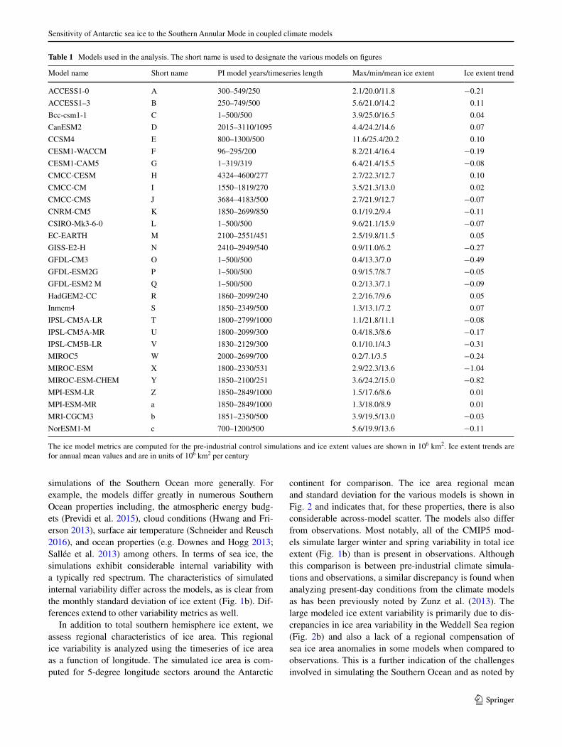
We assess CMIP5 pre-industrial (PI) control runs as listed in Table 1. As shown, the timeseries length is different across the various models. For our analysis, we use the longest timeseries possible from the different simulations. A number have sizable sea ice extent trends over the length of the PI timeseries indicating that they are not well equili-brated (Table 1; see also Turner et al. 2013a). We remove a linear trend from the ice extent timeseries prior to analysis. This may be problematic in some cases given that the equi-libration may not be linear. In general though, it does not qualitatively affect the results.

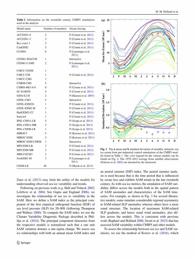
The annual cycle of pre-industrial southern hemisphere ice extent from the collection of CMIP5 simulations is shown in Fig. 1. As is clear, and noted in other studies (e.g. Turner et al. 2013a, 2015; Shu et al. 2015), the models differ considerably in their simulation of the mean Antarctic sea ice cover. Indeed considerable biases exist in climate model

Sensitivity of Antarctic sea ice to the Southern Annular Mode in coupled climate models

1 3

simulations of the Southern Ocean more generally. For example, the models differ greatly in numerous Southern Ocean properties including, the atmospheric energy budg-ets (Previdi et al. 2015), cloud conditions (Hwang and Fri-erson 2013), surface air temperature (Schneider and Reusch 2016), and ocean properties (e.g. Downes and Hogg 2013; Sallée et al. 2013) among others. In terms of sea ice, the simulations exhibit considerable internal variability with a typically red spectrum. The characteristics of simulated internal variability differ across the models, as is clear from the monthly standard deviation of ice extent (Fig. 1b). Dif-ferences extend to other variability metrics as well.

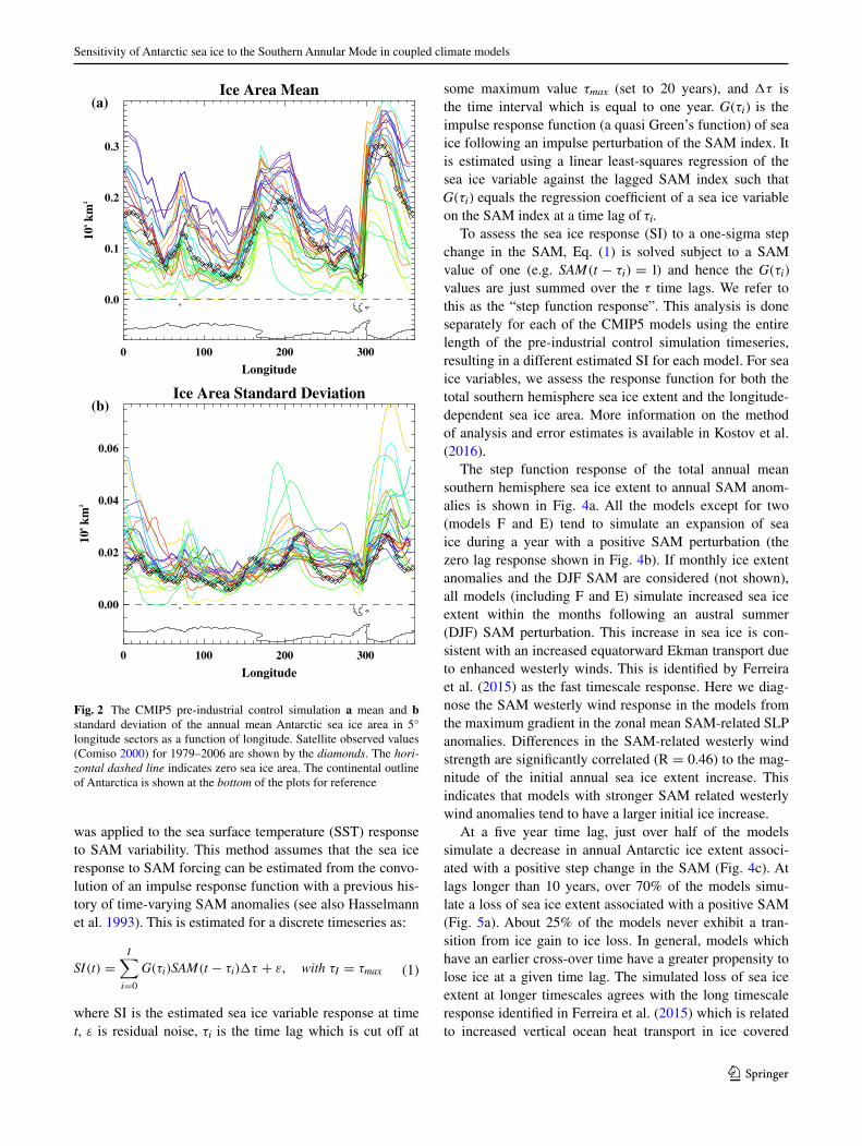
In addition to total southern hemisphere ice extent, we assess regional characteristics of ice area. This regional ice variability is analyzed using the timeseries of ice area as a function of longitude. The simulated ice area is com-puted for 5-degree longitude sectors around the Antarctic

continent for comparison. The ice area regional mean and standard deviation for the various models is shown in Fig. 2 and indicates that, for these properties, there is also considerable across-model scatter. The models also differ from observations. Most notably, all of the CMIP5 mod-els simulate larger winter and spring variability in total ice extent (Fig. 1b) than is present in observations. Although this comparison is between pre-industrial climate simula-tions and observations, a similar discrepancy is found when analyzing present-day conditions from the climate models as has been previously noted by Zunz et al. (2013). The large modeled ice extent variability is primarily due to dis-crepancies in ice area variability in the Weddell Sea region (Fig. 2b) and also a lack of a regional compensation of sea ice area anomalies in some models when compared to observations. This is a further indication of the challenges involved in simulating the Southern Ocean and as noted by

Table 1 Models used in the analysis. The short name is used to designate the various models on figures

The ice model metrics are computed for the pre-industrial control simulations and ice extent values are shown in 106 km2. Ice extent trends are for annual mean values and are in units of 106 km2 per century

Model name Short name PI model years/timeseries length Max/min/mean ice extent Ice extent trend

ACCESS1-0 A 300–549/250 2.1/20.0/11.8 −0.21

ACCESS1–3 B 250–749/500 5.6/21.0/14.2 0.11

Bcc-csm1-1 C 1–500/500 3.9/25.0/16.5 0.04

CanESM2 D 2015–3110/1095 4.4/24.2/14.6 0.07

CCSM4 E 800–1300/500 11.6/25.4/20.2 0.10

CESM1-WACCM F 96–295/200 8.2/21.4/16.4 −0.19

CESM1-CAM5 G 1–319/319 6.4/21.4/15.5 −0.08

CMCC-CESM H 4324–4600/277 2.7/22.3/12.7 0.10

CMCC-CM I 1550–1819/270 3.5/21.3/13.0 0.02

CMCC-CMS J 3684–4183/500 2.7/21.9/12.7 −0.07

CNRM-CM5 K 1850–2699/850 0.1/19.2/9.4 −0.11

CSIRO-Mk3-6-0 L 1–500/500 9.6/21.1/15.9 −0.07

EC-EARTH M 2100–2551/451 2.5/19.8/11.5 0.05

GISS-E2-H N 2410–2949/540 0.9/11.0/6.2 −0.27

GFDL-CM3 O 1–500/500 0.4/13.3/7.0 −0.49

GFDL-ESM2G P 1–500/500 0.9/15.7/8.7 −0.05

GFDL-ESM2 M Q 1–500/500 0.2/13.3/7.1 −0.09

HadGEM2-CC R 1860–2099/240 2.2/16.7/9.6 0.05

Inmcm4 S 1850–2349/500 1.3/13.1/7.2 0.07

IPSL-CM5A-LR T 1800–2799/1000 1.1/21.8/11.1 −0.08

IPSL-CM5A-MR U 1800–2099/300 0.4/18.3/8.6 −0.17

IPSL-CM5B-LR V 1830–2129/300 0.1/10.1/4.3 −0.31

MIROC5 W 2000–2699/700 0.2/7.1/3.5 −0.24

MIROC-ESM X 1800–2330/531 2.9/22.3/13.6 −1.04

MIROC-ESM-CHEM Y 1850–2100/251 3.6/24.2/15.0 −0.82

MPI-ESM-LR Z 1850–2849/1000 1.5/17.6/8.6 0.01

MPI-ESM-MR a 1850–2849/1000 1.3/18.0/8.9 0.01

MRI-CGCM3 b 1851–2350/500 3.9/19.5/13.0 −0.03

NorESM1-M c 700–1200/500 5.6/19.9/13.6 −0.11

M. M. Holland et al.

1 3

Zunz et al. (2013) may limit the utility of the models for understanding observed sea ice variability and trends.

Following on previous work (e.g. Hall and Visbeck 2002; Lefebvre et al. 2004; Sen Gupta and England 2006), we investigate the relationship of sea ice to variability in the SAM. Here we define a SAM index as the principal com-ponent of the first empirical orthogonal function (EOF) of sea level pressure (SLP) for 20–90S (following Thompson and Wallace 2000). To compute the SAM index we use the Climate Variability Diagnostic Package described in Phil-lips et al. (2014). The principal component timeseries from the respective models is normalized such that a one unit SAM variation denotes a one-sigma change. We assess sea ice relationships with both an annual mean SAM index and

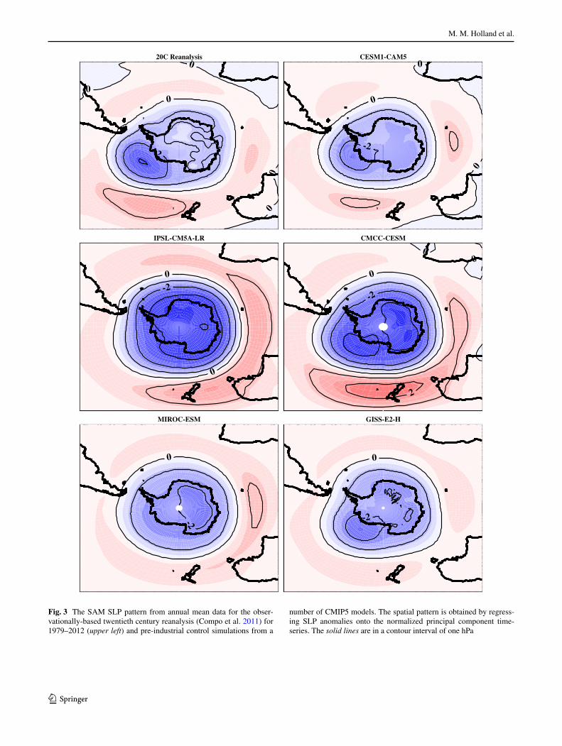
an austral summer (DJF) index. The austral summer analy-sis is used because that is the time period that is influenced by ozone loss and exhibits SAM trends in the late twentieth century. As with sea ice metrics, the simulation of SAM vari-ability differs across the models both in the spatial pattern of SAM anomalies and characteristics of the SAM time-series. For example, as shown in Fig. 3 for several illustra-tive models, some simulate considerable regional asymmetry in SAM-related SLP anomalies whereas others have a more zonal structure. The location of maximum SAM-related SLP gradients, and hence zonal wind anomalies, also dif-fers across the models. This is consistent with previous work (Raphael and Holland 2006; Swart et al. 2015) that has assessed SAM variability within CMIP5 and other models.

To assess the relationship between sea ice and SAM var-iations, we use the method of Kostov et al. (2016), which

Table 2 Information on the twentieth century CMIP5 simulations used in the analysis

Model name Number of members Ozone forcing

ACCESS1-0 2 P (Cionni et al. 2011)

ACCESS1-3 3 P (Cionni et al. 2011)

Bcc-csm1-1 3 P (Cionni et al. 2011)

CanESM2 5 P (Cionni et al. 2011)

CCSM4 6 P (Lamarque et al. 2011)

CESM1-WACCM 1 Interactive

CESM1-CAM5 2 P (Lamarque et al. 2011)

CMCC-CESM 1

CMCC-CM 1 P (Cionni et al. 2011)

CMCC-CMS 1

CNRM-CM5 5 Interactive

CSIRO-Mk3-6-0 8 P (Cionni et al. 2011)

EC-EARTH 5 P (Cionni et al. 2011)

GISS-E2-H 2 P (Hansen et al. 2007)

GFDL-CM3 5 Interactive

GFDL-ESM2G 1 P (Cionni et al. 2011)

GFDL-ESM2 M 1 P (Cionni et al. 2011)

HadGEM2-CC 1 P (Cionni et al. 2011)

Inmcm4 1 P (Cionni et al. 2011)

IPSL-CM5A-LR 5 P (Szopa et al. 2013)

IPSL-CM5A-MR 3 P (Szopa et al. 2013)

IPSL-CM5B-LR 1 P (Szopa et al. 2013)

MIROC5 5 P (Kawase et al. 2011)

MIROC-ESM 3 P (Kawase et al. 2011)

MIROC-ESM-CHEM 1 Interactive

MPI-ESM-LR 3 P (Cionni et al. 2011)

MPI-ESM-MR 3 P (Cionni et al. 2011)

MRI-CGCM3 3 P (Cionni et al. 2011)

NorESM1-M 3 P (Lamarque et al. 2011)

CESM-LE 40 P (Marsh et al. 2013)

J F M A M J J A S O N D

5

10

15

20

25

Mea

n Ic

e E

xten

t (1

06 km

2 )

J F M A M J J A S O N D

0.5

1.0

1.5

2.0

Stan

dard

Dev

iati

on (

106 k

m2 )

(a)

(b)

Fig. 1 The a mean and b standard deviation of monthly Antarctic sea ice extent from pre-industrial control simulations of the CMIP5 mod-els listed in Table 1. The color legend for the various models can be found on Fig. 4. The 1979–2012 average from satellite observations (Fetterer et al. 2002) are denoted by the diamonds

Sensitivity of Antarctic sea ice to the Southern Annular Mode in coupled climate models

1 3

was applied to the sea surface temperature (SST) response to SAM variability. This method assumes that the sea ice response to SAM forcing can be estimated from the convo-lution of an impulse response function with a previous his-tory of time-varying SAM anomalies (see also Hasselmann et al. 1993). This is estimated for a discrete timeseries as:

where SI is the estimated sea ice variable response at time t, ε is residual noise, τi is the time lag which is cut off at

(1)SI(t) =

I∑

i=0

G(τi)SAM(t − τi)�τ + ε, with τI = τmax

some maximum value τmax (set to 20 years), and �τ is the time interval which is equal to one year. G(τi) is the impulse response function (a quasi Green’s function) of sea ice following an impulse perturbation of the SAM index. It is estimated using a linear least-squares regression of the sea ice variable against the lagged SAM index such that G(τi) equals the regression coefficient of a sea ice variable on the SAM index at a time lag of τi.

To assess the sea ice response (SI) to a one-sigma step change in the SAM, Eq. (1) is solved subject to a SAM value of one (e.g. SAM(t − τi) = 1) and hence the G(τi) values are just summed over the τ time lags. We refer to this as the “step function response”. This analysis is done separately for each of the CMIP5 models using the entire length of the pre-industrial control simulation timeseries, resulting in a different estimated SI for each model. For sea ice variables, we assess the response function for both the total southern hemisphere sea ice extent and the longitude-dependent sea ice area. More information on the method of analysis and error estimates is available in Kostov et al. (2016).

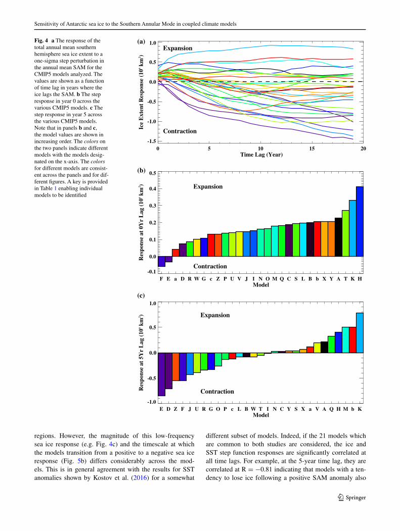
The step function response of the total annual mean southern hemisphere sea ice extent to annual SAM anom-alies is shown in Fig. 4a. All the models except for two (models F and E) tend to simulate an expansion of sea ice during a year with a positive SAM perturbation (the zero lag response shown in Fig. 4b). If monthly ice extent anomalies and the DJF SAM are considered (not shown), all models (including F and E) simulate increased sea ice extent within the months following an austral summer (DJF) SAM perturbation. This increase in sea ice is con-sistent with an increased equatorward Ekman transport due to enhanced westerly winds. This is identified by Ferreira et al. (2015) as the fast timescale response. Here we diag-nose the SAM westerly wind response in the models from the maximum gradient in the zonal mean SAM-related SLP anomalies. Differences in the SAM-related westerly wind strength are significantly correlated (R = 0.46) to the mag-nitude of the initial annual sea ice extent increase. This indicates that models with stronger SAM related westerly wind anomalies tend to have a larger initial ice increase.

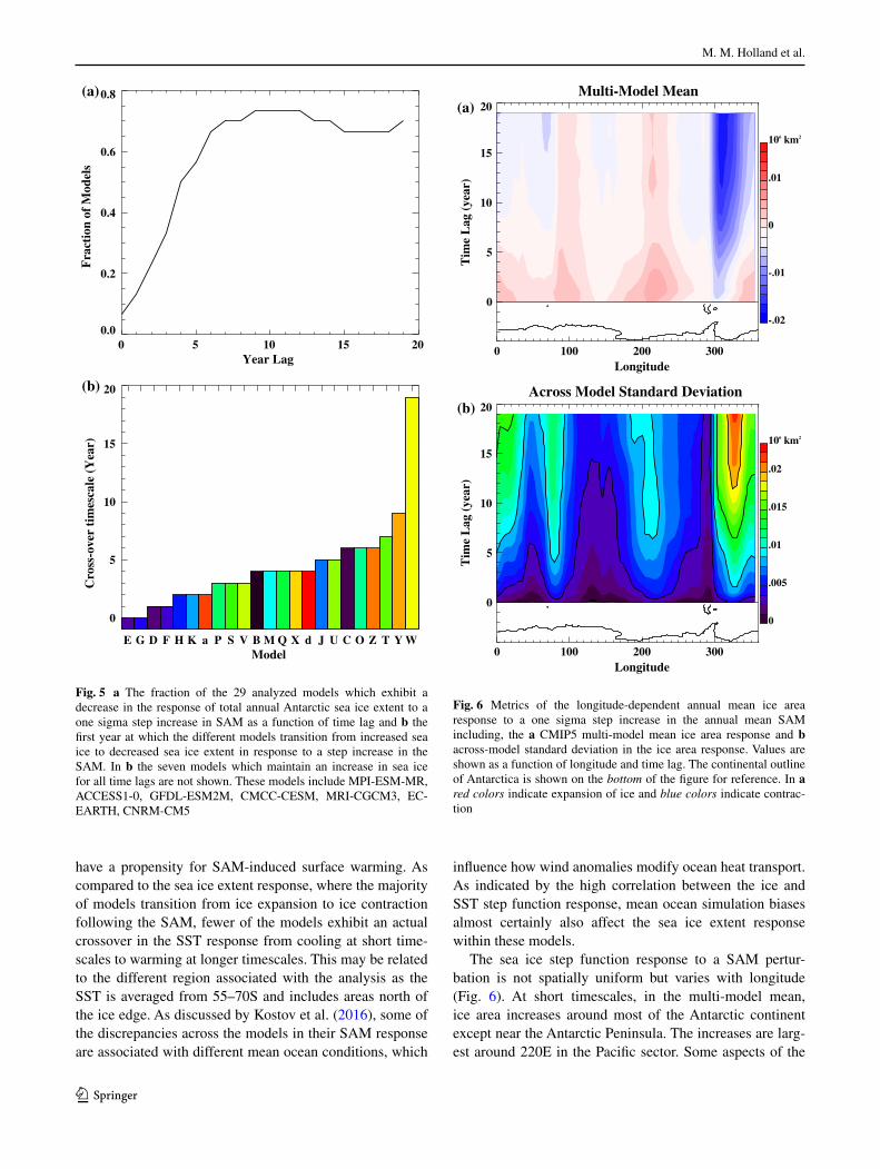
At a five year time lag, just over half of the models simulate a decrease in annual Antarctic ice extent associ-ated with a positive step change in the SAM (Fig. 4c). At lags longer than 10 years, over 70% of the models simu-late a loss of sea ice extent associated with a positive SAM (Fig. 5a). About 25% of the models never exhibit a tran-sition from ice gain to ice loss. In general, models which have an earlier cross-over time have a greater propensity to lose ice at a given time lag. The simulated loss of sea ice extent at longer timescales agrees with the long timescale response identified in Ferreira et al. (2015) which is related to increased vertical ocean heat transport in ice covered

Ice Area Mean

0 100 200 300

Longitude

0.0

0.1

0.2

0.3

106 k

m2

Ice Area Standard Deviation

0 100 200 300

Longitude

0.00

0.02

0.04

0.06

106 k

m2

(a)

(b)

Fig. 2 The CMIP5 pre-industrial control simulation a mean and b standard deviation of the annual mean Antarctic sea ice area in 5° longitude sectors as a function of longitude. Satellite observed values (Comiso 2000) for 1979–2006 are shown by the diamonds. The hori-zontal dashed line indicates zero sea ice area. The continental outline of Antarctica is shown at the bottom of the plots for reference

M. M. Holland et al.

1 3

20C Reanalysis

-2

0

0

00

0

CESM1-CAM5

-2

0

0

0

IPSL-CM5A-LR

-20

0

CMCC-CESM

-2

0

00

2

MIROC-ESM

-2

0

GISS-E2-H

-2

0

Fig. 3 The SAM SLP pattern from annual mean data for the obser-vationally-based twentieth century reanalysis (Compo et al. 2011) for 1979–2012 (upper left) and pre-industrial control simulations from a

number of CMIP5 models. The spatial pattern is obtained by regress-ing SLP anomalies onto the normalized principal component time-series. The solid lines are in a contour interval of one hPa

Sensitivity of Antarctic sea ice to the Southern Annular Mode in coupled climate models

1 3

regions. However, the magnitude of this low-frequency sea ice response (e.g. Fig. 4c) and the timescale at which the models transition from a positive to a negative sea ice response (Fig. 5b) differs considerably across the mod-els. This is in general agreement with the results for SST anomalies shown by Kostov et al. (2016) for a somewhat

different subset of models. Indeed, if the 21 models which are common to both studies are considered, the ice and SST step function responses are significantly correlated at all time lags. For example, at the 5-year time lag, they are correlated at R = −0.81 indicating that models with a ten-dency to lose ice following a positive SAM anomaly also

Fig. 4 a The response of the total annual mean southern hemisphere sea ice extent to a one-sigma step perturbation in the annual mean SAM for the CMIP5 models analyzed. The values are shown as a function of time lag in years where the ice lags the SAM. b The step response in year 0 across the various CMIP5 models. c The step response in year 5 across the various CMIP5 models. Note that in panels b and c, the model values are shown in increasing order. The colors on the two panels indicate different models with the models desig-nated on the x-axis. The colors for different models are consist-ent across the panels and for dif-ferent figures. A key is provided in Table 1 enabling individual models to be identified

0 5 10 15 20Time Lag (Year)

-1.5

-1.0

-0.5

0.0

0.5

1.0

Ice

Ext

ent

Res

pons

e (1

06 km

2 )

Expansion

Contraction

F E a D R W G c Z P U V J I N O M Q C S L B b X Y A T K HModel

-0.1

0.0

0.1

0.2

0.3

0.4

0.5

Res

pons

e at

0Y

r L

ag (

106 k

m2 ) Expansion

Contraction

E D Z F J U R G O P c L B W T I N C Y S X a V A Q H M b KModel

-1.0

-0.5

0.0

0.5

1.0

Res

pons

e at

5Y

r L

ag (

106 k

m2 ) Expansion

Contraction

(a)

(b)

(c)

M. M. Holland et al.

1 3

have a propensity for SAM-induced surface warming. As compared to the sea ice extent response, where the majority of models transition from ice expansion to ice contraction following the SAM, fewer of the models exhibit an actual crossover in the SST response from cooling at short time-scales to warming at longer timescales. This may be related to the different region associated with the analysis as the SST is averaged from 55–70S and includes areas north of the ice edge. As discussed by Kostov et al. (2016), some of the discrepancies across the models in their SAM response are associated with different mean ocean conditions, which

influence how wind anomalies modify ocean heat transport. As indicated by the high correlation between the ice and SST step function response, mean ocean simulation biases almost certainly also affect the sea ice extent response within these models.

The sea ice step function response to a SAM pertur-bation is not spatially uniform but varies with longitude (Fig. 6). At short timescales, in the multi-model mean, ice area increases around most of the Antarctic continent except near the Antarctic Peninsula. The increases are larg-est around 220E in the Pacific sector. Some aspects of the

0 5 10 15 20Year Lag

0.0

0.2

0.4

0.6

0.8F

ract

ion

of M

odel

s

E G D F H K a P S V B M Q X d J U C O Z T Y WModel

0

5

10

15

20

Cro

ss-o

ver

tim

esca

le (

Yea

r)(a)

(b)

Fig. 5 a The fraction of the 29 analyzed models which exhibit a decrease in the response of total annual Antarctic sea ice extent to a one sigma step increase in SAM as a function of time lag and b the first year at which the different models transition from increased sea ice to decreased sea ice extent in response to a step increase in the SAM. In b the seven models which maintain an increase in sea ice for all time lags are not shown. These models include MPI-ESM-MR, ACCESS1-0, GFDL-ESM2M, CMCC-CESM, MRI-CGCM3, EC-EARTH, CNRM-CM5

Multi-Model Mean

0 100 200 300Longitude

0

5

10

15

20

Tim

e L

ag (

year

)

-.02

-.01

0

.01

106 km2

Across Model Standard Deviation

0 100 200 300Longitude

0

5

10

15

20

Tim

e L

ag (

year

)

0

.005

.01

.015

.02

106 km2

(a)

(b)

Fig. 6 Metrics of the longitude-dependent annual mean ice area response to a one sigma step increase in the annual mean SAM including, the a CMIP5 multi-model mean ice area response and b across-model standard deviation in the ice area response. Values are shown as a function of longitude and time lag. The continental outline of Antarctica is shown on the bottom of the figure for reference. In a red colors indicate expansion of ice and blue colors indicate contrac-tion

Sensitivity of Antarctic sea ice to the Southern Annular Mode in coupled climate models

1 3

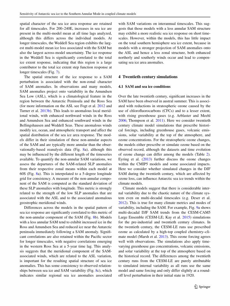
spatial character of the sea ice area response are retained for all timescales. For 200–240E, increases in sea ice are present in the multi-model mean at all time lags analyzed, although this differs across the individual models. At longer timescales, the Weddell Sea region exhibits the larg-est multi-model mean ice loss associated with the SAM but also the largest across-model uncertainty. The ice response in the Weddell Sea is significantly correlated to the total ice extent response, indicating that this region is a large contributor to the total ice extent step function response at longer timescales (Fig. 7).

The spatial structure of the ice response to a SAM perturbation is associated with the non-zonal character of SAM anomalies. In observations and many models, SAM anomalies project onto variability in the Amundsen Sea Low (ASL), which is a climatological feature in the region between the Antarctic Peninsula and the Ross Sea (for more information on the ASL see Fogt et al. 2012 and Turner et al. 2013b). This leads to anomalous local merid-ional winds, with enhanced northward winds in the Ross and Amundsen Sea and enhanced southward winds in the Bellingshausen and Weddell Seas. These anomalous winds modify ice, ocean, and atmospheric transport and affect the spatial distribution of the sea ice area response. The mod-els differ in their simulation of these non-annular aspects of the SAM and are typically more annular than the obser-vationally-based reanalysis data (Fig. 8a), although this may be influenced by the different length of the timeseries available. To quantify the non-annular SAM variations, we assess the departures of the SAM-related SLP anomalies from their respective zonal means within each model at 60S (Fig. 8a). This is interpolated to a 5-degree longitude grid for consistency. A measure of the non-annular compo-nent of the SAM is computed as the standard deviation of these SLP anomalies with longitude. This metric is strongly related to the strength of the low SLP anomalies that are associated with the ASL and to the associated anomalous geostrophic meridional winds.

Differences across the models in the spatial pattern of sea ice response are significantly correlated to this metric of the non-annular component of the SAM (Fig. 8b). Models with a less annular SAM tend to exhibit increased ice in the Ross and Amundsen Sea and reduced ice near the Antarctic peninsula immediately following a SAM anomaly. Signifi-cant correlations are also retained within the Pacific sector for longer timescales, with negative correlations emerging in the western Ross Sea at a 5-year time lag. This analy-sis suggests that the meridional component of the SAM-associated winds, which are related to the ASL variation, is important for the resulting spatial structure of sea ice anomalies. This has some consistency to observed relation-ships between sea ice and SAM variability (Fig. 8c), which indicates similar regional sea ice anomalies associated

with SAM variations on interannual timescales. This sug-gests that those models with a less annular SAM structure may exhibit a more realistic sea ice response on short time-scales. However, within the models, this has little impact on the total southern hemisphere sea ice extent, because in models with a stronger projection of SAM anomalies onto the ASL and hence a less zonal structure, both enhanced northerly and southerly winds occur and lead to compen-sating sea ice area anomalies.

4 Twentieth century simulations

4.1 SAM and sea ice conditions

Over the late twentieth century, significant increases in the SAM have been observed in austral summer. This is associ-ated with reductions in stratospheric ozone caused by the use of chlorofluorocarbons (CFCs) and to a lesser extent, with rising greenhouse gases (e.g. Arblaster and Meehl 2006; Thompson et al. 2011). Here we consider twentieth century climate model simulations that prescribe histori-cal forcings, including greenhouse gases, volcanic emis-sions, solar variability at the top of the atmosphere, and ozone concentrations. For the stratospheric ozone changes, the models either prescribe or simulate ozone based on the observed record, although the datasets and time evolution of ozone change can differ among the models (Table 2). Eyring et al. (2013) further discuss the ozone changes within the CMIP5 models and some associated impacts. Here we consider whether simulated changes in the DJF SAM during the twentieth century, which are affected by ozone loss, can influence Antarctic sea ice trends within the climate models.

Climate models suggest that there is considerable inter-nal variability due to the chaotic nature of the climate sys-tem even on multi-decadal timescales (e.g. Deser et al. 2012). This is true for many climate metrics and modes of variability, including the SAM. For example, Fig. 9a shows multi-decadal DJF SAM trends from the CESM-CAM5 Large Ensemble (CESM-LE; Kay et al. 2015) simulations for the pre-industrial and twentieth century climates. In the twentieth century, the CESM-LE runs use prescribed ozone as calculated by a high-top coupled chemistry–cli-mate model (Marsh et al. 2013). This ozone forcing agrees well with observations. The simulations also apply time-varying greenhouse gas concentrations, volcanic emissions, and solar variability at the top of the atmosphere based on the historical record. The differences among the twentieth century runs from the CESM-LE are purely attributable to simulated internal variability as all runs use the same model and same forcing and only differ slightly at a round-off level perturbation in their initial state in 1920.

M. M. Holland et al.

1 3

20C Reanalysis

-1.0

0.5

0.5

0.5

CESM1-CAM5

IPSL-CM5A-LR

0.5

CMCC-CESM

0.5

0.50.5

MIROC-ESM GISS-E2-H

Fig. 7 The non-annular component of the annual SAM from the twentieth century reanalysis (upper left panel) for 1979–2012 and some select models consistent with Fig. 3. The non-annular compo-

nent is computed as the difference of the SAM-related SLP anomalies from their zonal mean. The lined contour interval is 0.5 hPa and the zero contour is not shown. The dotted line indicates 60S latitude

Sensitivity of Antarctic sea ice to the Southern Annular Mode in coupled climate models

1 3

In response to anthropogenic forcing, the CESM-LE DJF SAM trends exhibit a discernible shift to positive values in the late twentieth century, which is consistent with the observed trend (Fig. 9a). The simulated mean trend for the

1975–2004 period is significantly different from zero at the 95% level. However, internal variability as diagnosed from the spread of trends across different ensemble members is still considerable, with a range of trends from −0.009 to

Fig. 8 a The SAM-associated SLP at 60S for the PI control simulations of the CMIP5 models (colored lines) and from the twentieth Century reanalysis (black dash line) and the ERA-Interim reanalysis data (Dee et al. 2011; black line). The reanalysis data are computed for 1979–2012. b The correlation of the ice area step function as a function of longitude with a metric of the non-annular com-ponent of the SAM as described in the text. Analysis is shown for the step function at 1 year lag (black) and 5 years lag (red). Values significant at the 95% level are indicated by the diamonds. c The correlation of the observed annual 1979–2012 detrended longitudinal ice area with the annual detrended SAM index obtained from the ERA-Interim reanalysis (solid) and the twentieth century reanalysis (dash). The dashed line indi-cates the 95% significance level

0 100 200 300

Longitude

-2

-1

0

1

(hPa)

0 100 200 300

Longitude

-1.0

-0.5

0.0

0.5

1.0

Correlation

0 100 200 300

Longitude

-1.0

-0.5

0.0

0.5

1.0

Correlation

(a)

(b)

(c)

M. M. Holland et al.

1 3

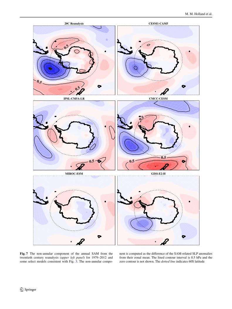
0.066 standard deviations per year across the members for 1975–2004. The CMIP5 models as a group also simulate a significant shift in the 30-year trends to positive values for the 1975–2004 period as compared to trends in their pre-industrial climates (Fig. 9b). The late twentieth century trend distribution is wider than the CESM-LE, with a range of −0.034 to 0.079 standard deviations per year for the 1975–2004 period. This wider spread is likely due in part to different prescribed forcing, including ozone, among the models and different model physics. However, as the comparison to CESM-LE suggests, internal variability also likely plays a large role in the variation in DJF SAM trends across the CMIP5 ensemble.

The distribution of annual sea ice extent trends from the CESM-LE and CMIP5 ensembles are shown in Fig. 10. As discussed in previous studies (Mahlstein et al. 2013; Turner et al. 2013a), the scatter in twentieth century sea ice trends across the climate models is large, with most simulations (and all members of the CESM-LE) showing ice loss over the 1975–2005 time period. This is in contrast to observa-tions, which show a small increasing trend in the total Ant-arctic sea ice extent over the satellite record since 1979 (e.g. Simmonds 2015). As indicated by the CESM-LE, internal variability can have a strong impact on the spread of trends from individual climate model realizations (see

-0.10 -0.05 0.00 0.05 0.10DJF SAM Trend

0.00

0.05

0.10

0.15

0.20

0.25

0.30F

requ

ency

of

Occ

urre

nce

-0.10 -0.05 0.00 0.05 0.10DJF SAM Trend

0.00

0.05

0.10

0.15

0.20

0.25

0.30

Fre

quen

cy o

f O

ccur

renc

e(a)

(b)

Fig. 9 The frequency of occurrence of 30 year trends in the DJF SAM timeseries from the a CESM-LE runs and b CMIP5 runs. The trends are in units of standard deviation per year. Shown are all pos-sible trends from the pre-industrial control runs (light grey), trends from ensemble members for 1975–2004 (black lines), and the 1979–2008 trend from the observationally-based twentieth century reanaly-sis (Compo et al. 2011) in red

-0.15 -0.10 -0.05 0.00 0.05 0.10 0.15Ice Trend (106 km2 per year)

0.00

0.05

0.10

0.15

0.20

0.25

0.30

Fre

quen

cy o

f O

ccur

renc

e

-0.15 -0.10 -0.05 0.00 0.05 0.10 0.15Ice Trend (106 km2 per year)

0.00

0.05

0.10

0.15

0.20

0.25

0.30

Fre

quen

cy o

f O

ccur

renc

e

(a)

(b)

Fig. 10 Thirty year trends in annual mean total Antarctic sea ice extent from a the CESM-LE and b the CMIP5 ensemble. The ice trends are in units of 106 km2 per year. The grey shading indicates the distribution of all possible 30 year trends in the pre-industrial control simulations. The black bars are the distribution of trends from 1975 to 2004. The red line shows the 1979–2008 observed trend (Fetterer et al. 2002) for reference. The dotted line indicates a trend of zero

Sensitivity of Antarctic sea ice to the Southern Annular Mode in coupled climate models

1 3

also Polvani and Smith 2013). This likely contributes to an important fraction of the spread in sea ice extent trends among the different CMIP5 models. However, given the wider spread in trends from the CMIP5 simulations, differ-ences in the prescribed external forcing and model struc-ture also likely contribute.

4.2 How are the twentieth century SAM timeseries and sea ice trends related?

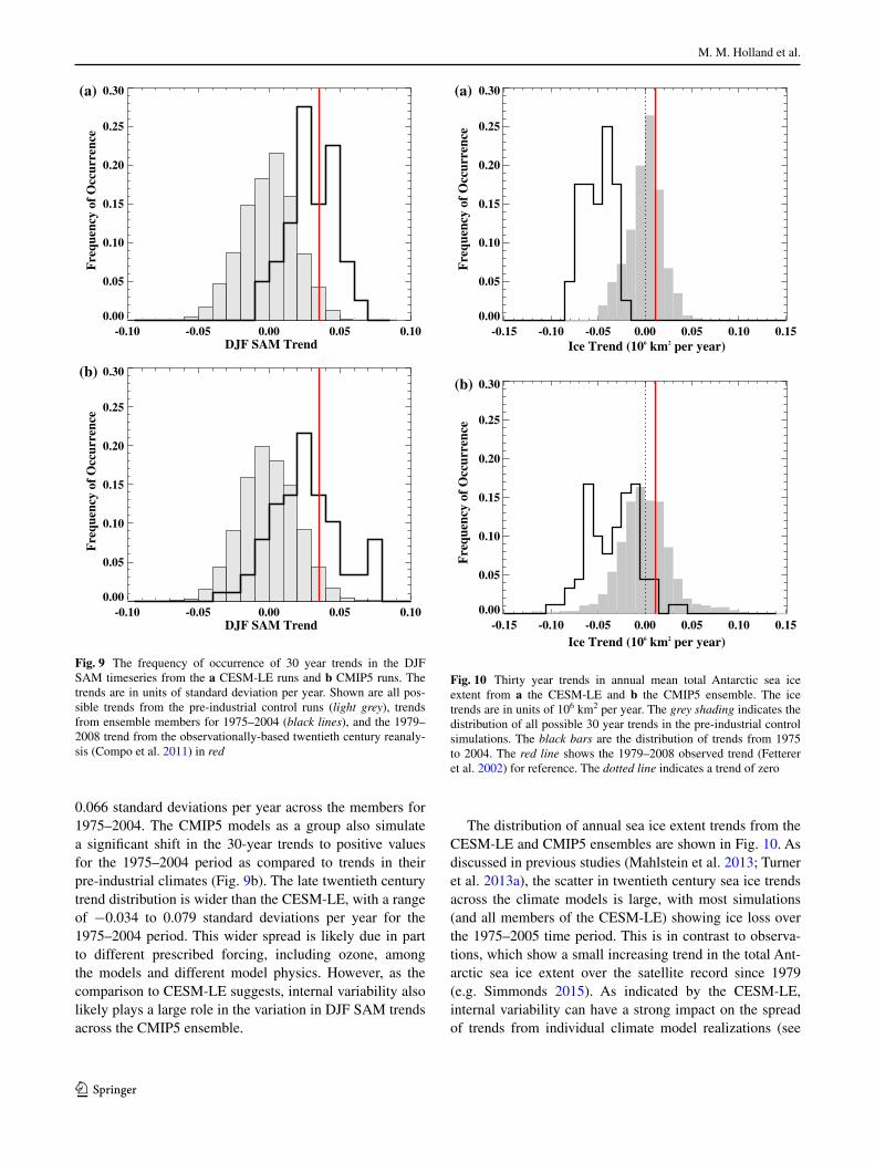
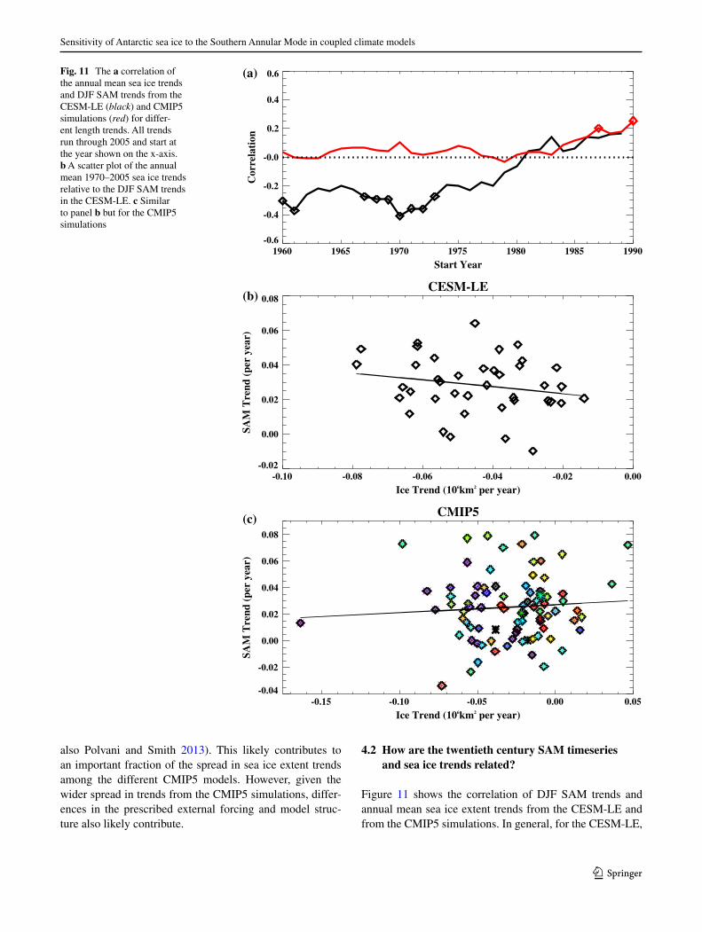
Figure 11 shows the correlation of DJF SAM trends and annual mean sea ice extent trends from the CESM-LE and from the CMIP5 simulations. In general, for the CESM-LE,

Fig. 11 The a correlation of the annual mean sea ice trends and DJF SAM trends from the CESM-LE (black) and CMIP5 simulations (red) for differ-ent length trends. All trends run through 2005 and start at the year shown on the x-axis. b A scatter plot of the annual mean 1970–2005 sea ice trends relative to the DJF SAM trends in the CESM-LE. c Similar to panel b but for the CMIP5 simulations

1960 1965 1970 1975 1980 1985 1990Start Year

-0.6

-0.4

-0.2

-0.0

0.2

0.4

0.6

Cor

rela

tion

CESM-LE

-0.10 -0.08 -0.06 -0.04 -0.02 0.00Ice Trend (106km2 per year)

-0.02

0.00

0.02

0.04

0.06

0.08

SAM

Tre

nd (

per

year

)

CMIP5

-0.15 -0.10 -0.05 0.00 0.05Ice Trend (106km2 per year)

-0.04

-0.02

0.00

0.02

0.04

0.06

0.08

SAM

Tre

nd (

per

year

)

(a)

(b)

(c)

M. M. Holland et al.

1 3

the spread in DJF SAM trends across the ensemble mem-bers is negatively correlated with the ice extent trends for timescales longer than about 25 years in the late twentieth century. These correlations only reach about 0.4, which is significant at the 95% level, but still quite small. Clearly other factors contribute to the spread in long-term sea ice trends across the CESM-LE members, but internal low-fre-quency variations in the SAM do appear to play a modest role. Members with larger DJF SAM trends tend to have enhanced ice loss in the twentieth century. This appears somewhat different from the analysis of the CMIP5 mod-els. When the collection of CMIP5 models is considered (Fig. 11c), little correlation exists between the DJF SAM trends and sea ice extent trends. Taken at face value, this suggests little influence of the SAM on sea ice trends within the twentieth century in the models.

However, as noted in Sect. 3, the models differ consid-erably in the simulated response of sea ice to a SAM per-turbation. We can account for this in the twentieth century simulations by convolving the twentieth century SAM timeseries with the response function obtained from the PI control runs. More specifically, we use Eq. (1) to provide an estimate of a sea ice property (SI) by multiplying the impulse response function (G(τi)) estimated from the PI control simulations by the time-varying twentieth century DJF SAM anomalies at the appropriate time lag and sum-ming this over the time lags. This means that the computed ice property is dependent on the prior 20 year evolution of SAM variations This provides an estimate of the sea ice variations in the twentieth century that can be attributed to the transient DJF SAM anomalies. This analysis is per-formed for all twentieth century ensemble members of the CMIP5 integrations that are available (Table 2) and for all members of the CESM-LE.

Figure 12 shows the correlation of the trends in the twentieth century annual mean Antarctic sea ice extent and the trends in the SAM-related sea ice extent response obtained through the convolution analysis. When the dif-ferent model responses to the SAM are accounted for, a significant relationship emerges for trends longer than about 20 years. This indicates that differences in the twen-tieth century transient SAM anomalies and the respective model responses to those anomalies are correlated with the spread of sea ice extent trends in the CMIP5 simulations at about R = 0.5. Comparing Figs. 11 and 12, the CESM-LE analysis also shows higher correlations for the convo-lution analysis. Given that all CESM-LE members use the same impulse response function (G(τi)) in the convolution analysis, this suggests that the transient nature of the SAM anomalies, and not just the linear trends, are important for the simulated sea ice response.

Assuming that the models simulate a realistic sea ice response to SAM variations, we should be able to obtain an

estimate of the effect of SAM variability on the observed sea ice by performing a similar convolution analysis using the modeled response function but subject to the observed SAM timeseries. This would account for both the effects of external forcings and the internal variability that occurred in the observed atmosphere. The convolution analysis approximates sea ice extent based on SAM conditions during the previous 20 years. As such, a long and consist-ent observationally-based SAM index is needed for this analysis (for example, to assess sea ice conditions start-ing in 1979, requires SAM information starting in 1960). This excludes the use of many reanalysis products because they are short in length and/or show spurious trends associ-ated with changing data input (e.g. Bromwich et al. 2007; Swart et al. 2015). As such, we perform the analysis using a SAM index derived from the twentieth century reanalysis (Compo et al. 2011), which assimilates only surface pres-sure observations. Prior to the International Geophysical Year in 1957, these observations were particularly sparse in the high southern latitudes leading to larger uncertainty in the reanalysis data and so we limit our analysis to the post 1957 period. To test the influence of the observationally-based data product, we repeat the analysis using a station-based estimate of the SAM index that is available since 1957 (Marshall 2003). For the period from 1957 to 2005, the DJF SAM timeseries from these two different datasets are correlated at R = 0.90.

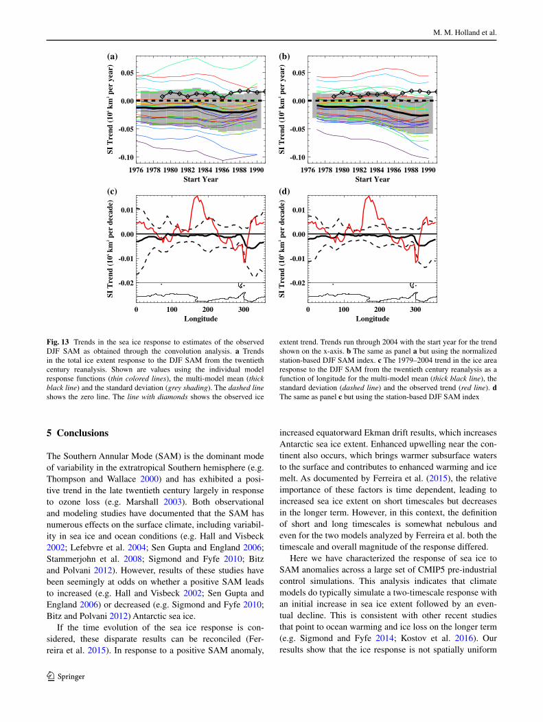
Shown in Fig. 13 is a convolution analysis using the two observationally-based estimates of the DJF SAM time-series for both the total Antarctic sea ice extent and the longitude dependent sea ice area response. The analysis is performed using the response functions from the indi-vidual models and then averaged to obtain a multi-model mean response. This multi-model mean response indicates DJF SAM-driven ice loss in the annual mean for total ice cover trends through 2005 and for ice area at essentially all longitudes for the 1979–2005 trends. However, as indi-cated on the figures, the uncertainty associated with the different response functions from the models is consider-able. Additional uncertainty arises from the determination of the observed SAM evolution. Comparing between the reanalysis and station-based SAM results (Fig. 13a–d), the trend in the sea ice response from 1979 to 2004 is typically larger when using the twentieth century reanalysis data. This is consistent with a larger DJF SAM trend in that data. However, this appears to be a considerably smaller source of uncertainty than the model response functions themselves.

Observed trends in sea ice are influenced by SAM-driven variations, the effects of other forcings, and internal variability. As such, a discrepancy between the observed trends and analysis shown in Fig. 13 could merely indi-cate the influence of non-SAM variations and may not

Sensitivity of Antarctic sea ice to the Southern Annular Mode in coupled climate models

1 3

necessarily indicate an issue with the models. Nevertheless, the observed trends generally are within the rather large standard deviation in the sea ice response trends from the convolution analysis. The primary exception to this is in the western Ross Sea region, where the observed trends are positive and well outside the multi-model spread. Notably,

observed ice trends within this region were also highlighted by Hobbs et al. (2015) as being outside simulated variabil-ity. This indicates that in the western Ross Sea either the model simulated response to the SAM is problematic or that other forcings are playing a strong role in the observed Ross Sea ice trends.

Fig. 12 The a correlation of the annual mean sea ice trends and trends in the SAM-related sea ice response obtained through a convolution analysis for the CESM-LE (black) and CMIP5 simulations (red). Correlations are computed for different length trends. All trends run through 2005 and start on the year shown on the x-axis. Sig-nificant values are indicated by the diamonds. b A scatter plot of the annual mean 1970–2005 sea ice trends and 1970–2005 trend in the SAM-related sea ice response for the CESM-LE. c Similar to panel b except for the CMIP5 simulations

1960 1965 1970 1975 1980 1985 1990

Start Year

-0.6

-0.4

-0.2

-0.0

0.2

0.4

0.6

Cor

rela

tion

CESM-LE

-0.10 -0.08 -0.06 -0.04 -0.02 0.00

Ice Trend (106km2 per year)

-0.05

-0.04

-0.03

-0.02

-0.01

0.00

0.01

SI T

rend

(10

6 km2 p

er y

ear)

CMIP5

-0.15 -0.10 -0.05 0.00 0.05

Ice Trend (106km2 per year)

-0.06

-0.04

-0.02

0.00

0.02

0.04

SI T

rend

(10

6 km2 p

er y

ear)

(a)

(b)

(c)

M. M. Holland et al.

1 3

5 Conclusions

The Southern Annular Mode (SAM) is the dominant mode of variability in the extratropical Southern hemisphere (e.g. Thompson and Wallace 2000) and has exhibited a posi-tive trend in the late twentieth century largely in response to ozone loss (e.g. Marshall 2003). Both observational and modeling studies have documented that the SAM has numerous effects on the surface climate, including variabil-ity in sea ice and ocean conditions (e.g. Hall and Visbeck 2002; Lefebvre et al. 2004; Sen Gupta and England 2006; Stammerjohn et al. 2008; Sigmond and Fyfe 2010; Bitz and Polvani 2012). However, results of these studies have been seemingly at odds on whether a positive SAM leads to increased (e.g. Hall and Visbeck 2002; Sen Gupta and England 2006) or decreased (e.g. Sigmond and Fyfe 2010; Bitz and Polvani 2012) Antarctic sea ice.

If the time evolution of the sea ice response is con-sidered, these disparate results can be reconciled (Fer-reira et al. 2015). In response to a positive SAM anomaly,

increased equatorward Ekman drift results, which increases Antarctic sea ice extent. Enhanced upwelling near the con-tinent also occurs, which brings warmer subsurface waters to the surface and contributes to enhanced warming and ice melt. As documented by Ferreira et al. (2015), the relative importance of these factors is time dependent, leading to increased sea ice extent on short timescales but decreases in the longer term. However, in this context, the definition of short and long timescales is somewhat nebulous and even for the two models analyzed by Ferreira et al. both the timescale and overall magnitude of the response differed.

Here we have characterized the response of sea ice to SAM anomalies across a large set of CMIP5 pre-industrial control simulations. This analysis indicates that climate models do typically simulate a two-timescale response with an initial increase in sea ice extent followed by an even-tual decline. This is consistent with other recent studies that point to ocean warming and ice loss on the longer term (e.g. Sigmond and Fyfe 2014; Kostov et al. 2016). Our results show that the ice response is not spatially uniform

1976 1978 1980 1982 1984 1986 1988 1990Start Year

-0.10

-0.05

0.00

0.05

SI T

rend

(10

6 km

2 per

yea

r)

1976 1978 1980 1982 1984 1986 1988 1990Start Year

-0.10

-0.05

0.00

0.05

SI T

rend

(10

6 km

2 per

yea

r)

0 100 200 300Longitude

-0.02

-0.01

0.00

0.01

SI T

rend

(10

6 km

2 per

dec

ade)

0 100 200 300Longitude

-0.02

-0.01

0.00

0.01

SI T

rend

(10

6 km

2 per

dec

ade)

(a) (b)

(c) (d)

Fig. 13 Trends in the sea ice response to estimates of the observed DJF SAM as obtained through the convolution analysis. a Trends in the total ice extent response to the DJF SAM from the twentieth century reanalysis. Shown are values using the individual model response functions (thin colored lines), the multi-model mean (thick black line) and the standard deviation (grey shading). The dashed line shows the zero line. The line with diamonds shows the observed ice

extent trend. Trends run through 2004 with the start year for the trend shown on the x-axis. b The same as panel a but using the normalized station-based DJF SAM index. c The 1979–2004 trend in the ice area response to the DJF SAM from the twentieth century reanalysis as a function of longitude for the multi-model mean (thick black line), the standard deviation (dashed line) and the observed trend (red line). d The same as panel c but using the station-based DJF SAM index

Sensitivity of Antarctic sea ice to the Southern Annular Mode in coupled climate models

1 3

however, with the Antarctic Peninsula region exhibiting decreases and the West Pacific region increases in sea ice area at all time lags in the multi-model mean response. After about 5 years, the ice area decreases in the Peninsula region extend to the entire Weddell Sea and dominate the total ice extent response, leading to the overall ice declines. Differences across the models in the regional character of sea ice change are associated with the non-annular structure of SAM anomalies, and in particular differences across the models in how SAM variability projects onto the Amund-sen Sea Low (ASL). As discussed by Hosking et al. (2013), many of the CMIP5 models simulate important biases in their depiction of the ASL, which could affect this aspect of the simulated sea ice forcing. However, while this is impor-tant for the spatial variations of the sea ice response, the resulting ice anomalies are largely compensating and so the non-annular structure of the simulated SAM has little influ-ence on the total ice extent response. At long timescales, the Weddell Sea region dominates the across-model uncer-tainty in the sea ice response indicating that simulating bet-ter conditions within this region is needed.

In response to a step increase in the SAM, the major-ity (about 70%) of the models transition from ice gain to ice loss within 7 years. However, this varies considerably across the models, with several models transitioning within the first year and others simulating ice gain for all time lags considered (out to 20 years). The magnitude of the initial ice extent gain is significantly related to the strength of the anomalous SAM-related westerlies, indicating that adequately simulating SAM characteristics is important for the ice response. A complementary study (Kostov et al. 2016), which considers the SST relationships to SAM vari-ations, also indicates that ocean model discrepancies are important in that different mean ocean conditions influence how effective anomalous winds are at driving ocean heat transport changes. A comparison to the Kostov et al. results suggests that these mean model biases also affect the sea ice response to the SAM. Our regional analysis indicates that biases within the Weddell Sea region may be particu-larly important for differences in the long timescale sea ice response across models.

The different model responses to SAM variations, as diagnosed from the pre-industrial control runs, have impli-cations for the transient climate response in the twentieth century. For the 1975–2004 period, the CMIP5 models simulate a discernible shift to positive SAM trends in the DJF season. This is consistent with prescribed or simu-lated ozone loss in the models. However, there is also a large spread in the trends across different simulations, much of which may be attributable to internal variability as diagnosed from a large ensemble of simulations from a single model. A simple correlation analysis suggests little influence of the different simulated SAM trends on sea ice

extent. However, if the different model SAM responses are accounted for, a significant relationship emerges. This indi-cates that different simulated transient SAM variations can account for a significant fraction of the late twentieth cen-tury spread in sea ice extent trends in the models provided that the different model responses are considered.

Consideration of the modeled SAM responses acting on the observed DJF SAM timeseries suggests that vari-ations in the observed SAM have contributed to a modest decrease in ice extent, with reductions occurring at all lon-gitudes, during the late twentieth century. However, given the large uncertainty in the modeled response to SAM vari-ations, the actual influence of SAM variations for twentieth century ice conditions remains unclear. Better constraints on the simulated sea ice response to the SAM are needed to more accurately simulate and understand its influence on trends in the Antarctic. As discussed by Kostov et al. (2016) biases in the mean ocean state appear to play an important role and should be the subject of future model improvements. Work also is needed to diagnose the rela-tive importance of other climate model biases and possible missing processes on the SAM response.

Acknowledgements The authors were supported under the NSF FESD program, Grant award #1338814. Y.K. received support from an NSF MOBY Grant, award #1048926. L.L. received sup-port from a NASA Grant, award NNX14AH74G. We acknowl-edge the World Climate Research Programme’s Working Group on Coupled Modelling, which is responsible for CMIP, and we thank the climate modeling groups (listed in Table 1 of this paper) for producing and making available their model output. For CMIP the U.S. Department of Energy’s Program for Climate Model Diagnosis and Intercomparison provides coordinating sup-port and led development of software infrastructure in partnership with the Global Organization for Earth System Science Portals. We also thank the CESM Large Ensemble Community Project and supercomputing resources provided by NSF/CISL/Yellowstone for providing the CESM-LE simulations. We also thank Dr. Peter Gent for comments on an earlier version of this manuscript.

References

Arblaster JM, Meehl GA (2006) Contributions of external forcings to Southern Annular Mode trends. J Clim 19:2896–2905

Bitz CM, Polvani LM (2012) Antarctic climate response to strato-spheric ozone depletion in a fine resolution ocean climate model. Geophys Res Lett. doi:10.1029/2012GL053393

Bromwich DH, Fogt RL, Hodges KI, Walsh JE (2007) A tropospheric assessment of the ERA-40, NCEP, and JRA-25 global reanalyses in the polar regions. J Geophys Res. doi:10.1029/2006JD007859

Cionni I, Eyring V, Lamarque JF, Randel WJ, Stevenson DS, Wu F, Bodeker GE, Shepherd TG, Shindell DT, Waugh DW (2011) Ozone database in support of CMIP5 simulations: results and corresponding radiative forcing. Atmos Chem Phys Discuss 11(4):10875–10933

Comiso JC (2000, updated 2015) Bootstrap sea ice concentrations from Nimbus-7 SMMR and DMSP SSM/I-SSMIS, version 2 [1979–2005]. Boulder, Colorado USA. NASA National Snow

M. M. Holland et al.

1 3

and Ice Data Center Distributed Active Archive Center. doi: http://dx.doi.org/10.5067/J6JQLS9EJ5HU

Compo GP et al (2011) The twentieth century reanalysis project. Q J R Meteorol Soc 137:1–28. doi:10.1002/qj.776

Dee DP et al (2011) The ERA-interim reanalysis: configuration and performance of the data assimilation system. QJR Meteorol Soc 137:553–597. doi:10.1002/qj.828

Deser C, Phillips A, Bourdette V, Teng H (2012) Uncertainty in cli-mate change projections: the role of internal variability. Clim Dyn 38:527–546. doi:10.1007/s00382-010-0977-x

Downes SM, Hogg AM (2013) Southern Ocean circulation and eddy compensation in CMIP5 models. J Clim 26(18):7198–7220

Eyring V et al (2013) Long-term ozone changes and associated cli-mate impacts in CMIP5 simulations. J Geophys Res Atmos 118:5029–5060. doi:10.1002/jgrd.50316

Ferreira D, Marshall J, Bitz CM, Solomon S, Plumb A (2015) Ant-arctic Ocean and sea ice response to ozone depletion: a two-time-scale problem. J Clim 28:1206–1226. doi:10.1175/JCLI-D-14-00313.1

Fetterer F, Knowles K, Meier W, Savoie M (2002) Sea Ice Index. National Snow and Ice Data Center, Boulder. doi:10.7265/N5QJ7F7W

Fogt RL, Wovrosh AJ, Langen RA, Simmond I (2012) The character-istic variability and connection to the underlying synoptic activ-ity of the Amundsen-Bellingshausen Seas Low. J Geophys Res 117:D07111. doi:10.1029/2011JD017337

Hall A, Visbeck M (2002) Synchronous variability in the Southern Hemisphere atmosphere, sea ice, and ocean resulting from the Annular Mode. J Clim 15:3043–3057

Hansen J et al (2007) Climate simulations for 1880–2003 with GISS modelE. Clim Dyn 29(7–8):661–696

Hasselmann K, Sausen R, Maier-Reimer E, Voss R (1993) On the cold start problem in transient simulations with coupled atmosphere-ocean models. Clim Dyn 9:53–61. doi:10.1007/BF00210008

Hobbs WR, Bindoff NL, Raphael MN (2015) New perspective on observed and simulated Antarctic sea ice extent trends using optimal fingerprinting techniques. J Clim 28:1543–1560. doi:10.1175/JCLI-D-14-00367.1

Hosking JS, Orr A, Marshall GJ, Turner J, Phillips T (2013) The influence of the Amundsen-Bellingshausen Seas low on the climate of West Antarctic and its representation in coupled cli-mate model simulations. J Clim 26:6633–6648. doi:10.1175/JCLI-D-12-00813.1

Hurrell JW et al (2013) The community earth system model: a frame-work for collaborative research. Bull Am Met Soc. doi:10.1175/BAMS-D-12-00121.1

Hwang YT, Frierson DMW (2013) A link between the double-intertropical convergence zone problem and cloud biases over the Southern Ocean. Proc Natl Acad Sci 110:4935–4940. doi:10.1073/pnas.1213302110

Kawase H, Nagashima T, Sudo K, Nozawa T (2011) Future changes in tropospheric ozone under representative concentration path-ways (RCPs). Geophys Res Lett 38:L05801. doi:10.1029/2010GL046402

Kay JE et al (2015) The community earth system model (CESM) large ensemble project: a community resource for study-ing climate change in the presence of internal climate vari-ability. Bull Am Met Soc 96:1333–1349. doi:10.1175/BAMS-D-13-00255.1

Knutti R, Masson D, Gettelman A (2013) Climate model genealogy: generation CMIP5 and how we got there. Geophys Res Lett 40:1194–1199. doi:10.1002/grl.50256

Kostov Y, Marshall J, Hausmann U, Armour KC, Ferreira D, Holland MM (2016) Fast and slow responses of Southern Ocean sea sur-face temperature to SAM in coupled climate models. Clim Dyn. doi:10.1007/s00382-016-3162-z

Kwok R, Comiso JC (2002) Spatial patterns of variability in Antarc-tic surface temperature: connections to the Southern Hemisphere Annular Mode and the southern oscillation. Geophy Res Lett. doi:10.1029/2002GL015415

Lamarque JF, Kyle GP, Meinshausen M, Riahi K, Smith SJ, van Vuuren DP, Conley AJ, Vitt F (2011) Global and regional evo-lution of short-lived radiatively-active gases and aerosols in the representative concentration pathways. Clim Chang 109:191–212

Lefebvre W, Goosse H, Timmermann R, Fichefet T (2004) Influence of the Southern Annular Mode on the sea ice–ocean system. J Geophys Res. doi:10.1029/2004JC002403

Mahlstein I, Gent PR, Solomon S (2013) Historical Antarctic mean sea ice area, sea ice trends, and winds in CMIP5 simulations. J Geophys Res Atmos 118:5105–5110. doi:10.1002/jgrd.50443

Marsh D, Mills M, Kinnison DE, Lamarque JF (2013) Climate change from 1850 to 2005 simulated in CESM1(WACCM). J Clim 26:7372–7391. doi:10.1175/JCLI-D-12-00558.1

Marshall GJ (2003) Trends in the Southern Annular Mode from observations and reanalyses. J Clim 16:4134–4143. doi:10.1175/1520-0442(2003)016<4134:TITSAM>2.0.CO;2

Pezza AB, Rashid HA, Simmonds I (2012) Climate links and recent extremes in Antarctic sea ice, high-latitude cyclones, Southern Annular Model and ENSO. Clim Dyn 38:57–73. doi:10.1007/s00382-011-1044-y

Phillips AS, Deser C, Fasullo J (2014) A new tool for evaluat-ing modes of variability in climate models. EOS 95:453–455. doi:10 .1002/2014EO490002

Polvani LM, Smith KL (2013) Can natural variability explains observed Antarctic sea ice trends? New modeling evidence from CMIP5. Geophys Res Lett 40:3195–3199. doi:10.1002/grl.50578

Previdi M, Smith KL, Polvani LM (2015) How well do the CMIP5 models simulate the Antarctic atmospheric energy budget? J Clim 28(20):7933–7942

Raphael M, Holland MM (2006) Twentieth century simulation of the Southern Hemisphere in coupled models. Part I: large scale circulation variability. Clim Dyn 26:217–228. doi:10.1007/s00382-005-0082-8

Sallée JB, Shuckburgh E, Bruneau N, Meijers AJS, Bracegirdle TJ, Wang Z, Roy T (2013) Assessment of Southern Ocean water mass circulation and characteristics in CMIP5 models: histori-cal bias and forcing response. J Geophys Res Oceans 118:1830–1844. doi:10.1002/jgrc.20135

Schneider DP, Reusch DB (2016) Antarctic and Southern Ocean sur-face temperatures in CMIP5 models in the context of the surface energy budget. J Clim 29(5):1689–1716

Sen Gupta A, England M (2006) Coupled ocean-atmosphere feedback in the Southern Annular Mode. J Clim 20:3677–3692

Shu Q, Song Z, Qiao F (2015) Assessment of sea ice simulations in the CMIP5 models. Cryosphere 9(1):399–409

Sigmond M, Fyfe JC (2010) Has the ozone hole contributed to increased Antarctic sea ice extent? Geophys Res Lett 37:L18502. doi:10.1029/2010GL044301

Sigmond M, Fyfe JC (2014) The Antarctic sea ice response to the ozone hole in climate models. J Clim 27:1336–1342. doi:10.1175/JCLI-D-13-00590.1

Simmonds I (2015) Comparing and contrasting the behavior of Arctic and Antarctic sea ice over the 35 year period 1979–2013. Ann Glaciol 56:18–28. doi:10.3189/2015AoG69A909

Simpkins GR, Ciasto LM, Thompson DWJ, England MH (2012) Seasonal relationships between large-scale climate variabil-ity and Antarctic sea ice concentration. J Clim 25:5451–5469. doi:10.1175/JCLI-D-11-00367.1

Smith KL, Polvani LM, Marsh DR (2012) Mitigation of 21st century Antarctic sea ice loss by stratospheric ozone recovery. Geophys Res Lett 39:L20701. doi:10.1029/2012GL053325

Sensitivity of Antarctic sea ice to the Southern Annular Mode in coupled climate models

1 3

Stammerjohn SE, Martinson DG, Smith RC, Yuan X, Rind D (2008) Trends in Antarctic annual sea ice retreat and advance and their relation to El Niño-Southern Oscillation and Southern Annular Mode variability. J Geophys Res 108:C03S90. doi:10.1029/2007JC004269

Swart NC, Fyfe JC, Gillett N, Marshall GJ (2015) Comparing trends in the Southern Annular Mode and surface westerly jet. J Clim 28:8840–8859. doi:10.1175/JCLI-D-15-0334.1

Szopa S et al (2013) Aerosol and ozone changes as forcing for climate evolution between 1850 and 2100. Clim Dyn 40:2223–2250. doi:10.1007/s00382-012-1408-y

Taylor KE, Stouffer RJ, Meehl GA (2012) An overview of CMIP5 and the experiment design. Bull Am Meteor Soc 93:485–498. doi:10.1175/BAMS-D-11-00094.1

Thompson DWJ, Solomon S (2002) Interpretation of recent South-ern Hemisphere climate change. Science 296(5569):895–899. doi:10.1126/science.1069270

Thompson DWJ, Wallace JM (2000) Annular modes in the extrat-ropical circulation. Part I: month-to month variability. J Clim 13:1000–1016

Thompson DWJ et al (2011) Signatures of the Antarctic ozone hole in Southern Hemisphere surface climate change. Nat Geosci 4:741749. doi:10.1038/ngeo1296

Turner J, Bracegirdle TJ, Phillips T, Marshall GJ, Hosking JS (2013a) An initial assessment of Antarctic sea ice extent in the CMIP5 models. J Clim 26:1473–1484. doi:10.1175/JCLI-D-12-00068.1

Turner J, Phillips T, Hosking JS, Marshall GJ, Orr A (2013b) The Amundsen Sea Low. Int J Climatol 33:1818–1829. doi:10.1002/joc.3558

Turner J, Hosking JS, Bracegirdle TJ, Marshall GJ, Phillips T (2015) Recent changes in Antarctic sea ice. Phil Trans R Soc A 373:20140163. doi:10.1098/rsta.2014.0163

Zunz V, Goosse H, Massonnet F (2013) How does internal variability influence the ability of CMIP5 models to reproduce the recent trend in Southern Ocean sea ice extent? Cryosphere 7:451–468. doi:10.5194/tc-7-451-2013