seminario dottorato 2014/15 · universit a di padova { dipartimento di matematica scuole di...
TRANSCRIPT
Universita di Padova – Dipartimento di Matematica
Scuole di Dottorato in Matematica Pura, Matematica Computazionale e Informatica
Seminario Dottorato 2014/15
Preface 2
Abstracts (from Seminario Dottorato’s web page) 3
Notes of the seminars 8
Matteo Basei, The stochastic mesh method to price American options and swing contracts . . . 8Joao Meireles, Singular perturbations of stochastic control problems with unbounded fast variables 18Paolo Pigato, An introduction to density estimates for diffusion processes . . . . . . . . . . . . 24Genaro Hernandez Mada, Semistable degenerations of K3 surfaces . . . . . . . . . . . . . . . 33Davide Buoso, Shape sensitivity analysis for vibrating plate models . . . . . . . . . . . . . . . . 42Sander Dommers, Metastability of the Ising model on random graphs at zero temperature . . . . 47Nguyen Khanh Tung, Automorphism-invariant modules . . . . . . . . . . . . . . . . . . . . . . 56Gabriele Santin, Introduction to kernel-based methods . . . . . . . . . . . . . . . . . . . . . . . 64Velibor Bojkovic, A short introduction to Berkovich affine line over the field Cp . . . . . . . . 70Aigul Myrzagaliyeva, On differential operators and multipliers in weighted Sobolev spaces . . 80Cristina Cornelio, Preferences in AI . . . . . . . . . . . . . . . . . . . . . . . . . . . . . . . . 90Alice Fiaschi, Variational methods in Nonlinear Elasticity: an introduction . . . . . . . . . . . 98Thuy T.T. Le, Controllability and the numerical approximation of the minimum time function . 107Francesco Mattiello, An introduction to derived categories . . . . . . . . . . . . . . . . . . . 119Federico Piazzon, Why should people in approximation theory care about (pluri-)potential theory? 134
1
Seminario Dottorato 2014/15
Preface
This document offers a large overview of the eight months’ schedule of Seminario Dottorato2014/15. Our “Seminario Dottorato” (Graduate Seminar) is a double-aimed activity. Atone hand, the speakers (usually Ph.D. students or post-docs, but sometimes also seniorresearchers) are invited to think how to communicate their researches to a public of math-ematically well-educated but not specialist people, by preserving both understandabilityand the flavour of a research report. At the same time, people in the audience enjoy arare opportunity to get an accessible but also precise idea of what’s going on in somemathematical research area that they might not know very well.Let us take this opportunity to warmly thank the speakers once again, in particular fortheir nice agreement to write down these notes to leave a concrete footstep of their par-ticipation. We are also grateful to the collegues who helped us, through their advices andsuggestions, in building an interesting and culturally complete program.
Padova, July 2nd, 2015
Corrado Marastoni, Tiziano Vargiolu
Universita di Padova – Dipartimento di Matematica 2
Seminario Dottorato 2014/15
Abstracts (from Seminario Dottorato’s web page)
Wednesday 5 November 2014
The stochastic mesh method to price swing contracts
Matteo BASEI (Padova, Dip. Mat.)
This talk is based on the results achieved during a six-month internship in the Risk Department
of a leading energy company. Our goal is twofold: on the one hand we give a brief survey on
the problem of pricing swing contracts by the stochastic mesh method, on the other hand we
describe our experience in the use of advanced mathematics in a private company. Firstly, we
consider the case of American options and study the original formulation of the stochastic mesh
method, introduced by Broadie and Glasserman in 1997. Secondly, we try to improve the method
by optimally calibrating the parameters, by a literature review and by the use of variance reduction
techniques. Finally, we use the revised method to price swing options in energy markets.
Wednesday 19 November 2014
Singular perturbations of stochastic control problems with unbounded fast variables
Joao MEIRELES (Padova, Dip. Mat.)
In this talk, we first give a short introduction to singular perturbations problems and to the
Hamilton-Jacobi approach to the singular limit ε → 0. And we will end by considering a specific
singular perturbation problem of a class of optimal stochastic control problems with unbounded
fast variables and discussing some recents results.
Wednesday 26 November 2014
An introduction to density estimates for diffusions
Paolo PIGATO (Padova, Dip. Mat.)
We recall some notions in Malliavin calculus and some general criteria for the absolute continuity
and regularity of the density of a diffusion. We present some estimates for degenerate diffu-
sions under a weak Hormander condition, obtained by starting from the Malliavin and Thalmaier
representation formula for the density. As an example, we focus in particular on the stochastic
differential equation used to price Asian Options.
Universita di Padova – Dipartimento di Matematica 3
Seminario Dottorato 2014/15
Wednesday 17 December 2014
A gentle introduction to semistable degeneration of K3 surfaces
Genaro HERNANDEZ MADA (Padova, Dip. Mat.)
In this talk we give the elements to understand the definition and two results about semistable
degenerations of K3 surfaces over the complex numbers. The first result is a description of the
special fiber and the second one is a classification of it in terms of monodromy. If time allows, we
shall also introduce the p-adic analogue of these results.
Wednesday 28 January 2015
Shape sensitivity analysis for vibrating plate models
Davide BUOSO (Padova, Dip. Mat.)
In this talk, we consider two different models for the vibration of a clamped plate: the Kirchhoff-
Love model, which leads to the well known biharmonc operator, and the Reissner-Mindlin model,
which instead gives a system of differential equations. We point out similarities and differences,
showing the connections between these two problems. Then we show some results concerning
the stability of the spectrum with respect to domain perturbations. After recalling the known
results in shape optimization for the biharmomic operator, we state some analyticity results for
the dependence of the eigenvalues upon domain perturbations and Hadamard-type formulas for
shape derivatives. Using these formulas, we prove that balls are critical domains for the symmetric
functions of the eigenvalues under volume constraint.
Wednesday 11 February 2015
Metastability of the Ising model on random graphs at zero temperature
Sander DOMMERS (Bologna, Dip. Mat.)
In this talk I will introduce a random graph model known as the configuration model. After this,
I will discuss the Ising model, which is a model from statistical physics where a spin is assigned to
each vertex in a graph and these spins tend to align, i.e., take the same value as their neighbors. It
is especially interesting to study the Ising model on random graphs. I will discuss some properties
of this model. In particular, I will talk about the dynamics and metastability in this model when
the interaction strength goes to infinity. This corresponds to the zero temperature limit in physical
terms.
Universita di Padova – Dipartimento di Matematica 4
Seminario Dottorato 2014/15
Wednesday 25 February 2015
Automorphism-invariant modules
Khanh Tung NGUYEN (Padova, Dip. Mat.)
In this talk, after recalling some basic concepts, we mention the class of injective modules, the class
of quasi-injective modules and their generalization, the class of automorphism-invariant modules.
Next, we give some results related to the endomorphism rings of automophism-invariant modules
and their injective envelopes. Finally, we show a connection between automorphism-invariant
modules and bolean rings.
Wednesday 18 March 2015
Introduction to kernel-based methods
Gabriele SANTIN (Padova, Dip. Mat.)
In this talk we give an introduction to kernel-based methods and to their application in different
fields of applied mathematics. We consider some examples that motivate the use of kernel-based
techniques. Each example can be included in the same framework, but allows to show and discuss
different features that arise naturally in the particular application. The examples deal with mul-
tivariate scattered data approximation, optimal recovery in Hilbert spaces, numerical solution of
PDE, machine learning, and statistics. After building up the fundamental tools of kernel-based
methods, we will introduce the problem of the determination of optimal subspaces for kernel-
based multivariate approximation. We will give some insight into the problem and discuss possible
applications.
Wednesday 1 April 2015
Zooming into p-adic curves
Velibor BOJKOVIC (Padova, Dip. Mat.)
The goal of the seminar is to introduce the audience to the basic notions of Berkovich geometry
through a toy example of a p-adic projective curve. After recalling the basic properties of a p-adic
field, we motivate Vladimir Berkovich’s approach to studying geometry over such fields and go into
describing the structure of compact p-adic curves.
Universita di Padova – Dipartimento di Matematica 5
Seminario Dottorato 2014/15
Wednesday 15 April 2015
Sobolev spaces, differential operators and multipliers
Aigul MYRZAGALIYEVA (Padova, Dip. Mat. and Eurasian National Univ. Astana)
In this talk, after recalling some basic notions of Sobolev spaces we give some examples, then we
introduce differential operators and multipliers in pair of Sobolev spaces. We give the statement
and motivation of the problem. Morever, we also present some open problems.
Wednesday 29 April 2015
Preferences in AI
Cristina CORNELIO (Padova, Dip. Mat.)
Artificial Intelligence (AI) is a field that has a long history but still constantly and actively grow-
ing and changing. The applications of AI are several, for example web search, speech recognition,
face recognition, machine translation, autonomous driving, automatic scheduling etc. These are
all complex real-world problems, and the goal of artificial intelligence (AI) is to tackle these with
rigorous mathematical tools: machine learning, search, game playing, Markov decision processes,
constraint satisfaction, graphical models, and logic. Recently, a new concept became very im-
portant in AI: the use of preferences. Let’s think about social networks, online shops, systems
that suggest music or films. In this talk it is presented an overview on the main applications of
preferences in AI, like recommender systems, multi-agent decision making, computational social
choice, stable marriage problems, uncertainty in preferences and qualitative preferences.
Wednesday 6 May 2015
Variational methods in nonlinear elasticity: an introduction
Alice FIASCHI (Padova, Dip. Mat.)
After a brief introduction of the variational formulation for the standard model in nonlinear elas-
ticity, we will consider the problem of finding the “right” space to describe the equilibrium configu-
rations of an elastic body, from the point of view of the Calculus of Variations. In this framework,
I will introduce the space of Young measures as a suitable space to describe materials exhibiting
microstructures.
Universita di Padova – Dipartimento di Matematica 6
Seminario Dottorato 2014/15
Wednesday 27 May 2015
Controllability and the numerical approximation of the minimum time function
Thien Thuy LE THI (Padova, Dip. Mat.)
In optimal control theory, minimum time problems are of interest since they appear in many
applications such as robotics, automotive, car industry, etc.. The scope of this talk is to give a brief
introduction of these problems. Controllability conditions under various settings are considered.
Such conditions play a vital role in studying the regularity of the minimum time function T (x).
Moreover, we will also introduce the HJB equation associated with a minimum time problem and
approaches to computing T (x) approximately.
Wednesday 10 June 2015
An introduction to derived categories
Francesco MATTIELLO (Padova, Dip. Mat.)
Derived categories were introduced in the sixties by Grothendieck and Verdier and have proved to
be of fundamental importance in Mathematics. Starting with a short review of the basic language
of category theory, we will first introduce the notion of abelian category with the help of several
examples. Then we will spend some time giving a thorough motivation for the construction of the
derived category of an abelian category. Finally, we will look at a way to break a derived category
into two pieces that permit (among other things) to recover the original abelian category.
Wednesday 24 June 2015
Why should people in approximation theory care about (pluri-)potential theory?
Federico PIAZZON (Padova, Dip. Mat.)
We give an introductory summary of results in (pluri-)potential theory that naturally come into
play when considering classical approximation theory issues both in one and (very concisely) in sev-
eral complex variables. We focus on Fekete points and the asymptotic of orthonormal polynomials
for certain L2 counterpart of Fekete measures. No specific knowledge on the topic is assumed.
Universita di Padova – Dipartimento di Matematica 7
Seminario Dottorato 2014/15
The stochastic mesh method to price
American options and swing contracts
Matteo Basei (∗)
Abstract. This talk is based on the results achieved during a six-month internship in the RiskDepartment of a leading energy company. Our goal is twofold: on the one hand we give a briefsurvey on the problem of pricing swing contracts by the stochastic mesh method, on the otherhand we describe our experience in the use of advanced mathematics in a private company.Firstly, we consider the case of American options and study the original formulation of the stochas-tic mesh method, introduced by Broadie and Glasserman in 1997. Secondly, we try to improve themethod by optimally calibrating the parameters, by a literature review and by the use of variancereduction techniques. Finally, we outline how to use the method to price swing options in energymarkets.
Contents
1. Introduction . . . . . . . . . . . . . . . . . . . . . . . . . . . . . . . . . . . . . . . . . . . . . . . . . . . . . . . . . . . . . . . . . . . 82. Pricing American options by the stochastic mesh method . . . . . . . . . . . . . . . . . . . . . 103. Improving the method . . . . . . . . . . . . . . . . . . . . . . . . . . . . . . . . . . . . . . . . . . . . . . . . . . . . . . . . 154. Pricing swing options by the stochastic mesh method . . . . . . . . . . . . . . . . . . . . . . . . . 15
1 Introduction
We here give the definitions of European and American options and outline some featuresof energy markets.
European and American options. The following definitions are fundamental inmathematical finance.
- A European option is a contract giving the holder the right (not the obligation!) tobuy or sell an underlying asset at a prespecified price and on a prespecified date.
(∗)Ph.D. course, Universita di Padova, Dip. Matematica, via Trieste 63, I-35121 Padova, Italy; E-mail:. Seminar held on November 5th, 2014.
Universita di Padova – Dipartimento di Matematica 8
Seminario Dottorato 2014/15
Example. We have the right to buy one UniPd stock at 10e on 10th November. Onthat date, we check the price of one UniPd stock; if the price is less than 10e, wedo not exercise the option, if the price is greater than 10e (say 15e), we do exercisethe option (the gain being 15-10=5e).
- An American option is similar to a European option, but here the holder can choose,among a set of prespecified dates, when to exercise the right.
Example. We have the right to buy one UniPd stock at 10e on 10th, 11th, 12th or13th November. On those dates, we check the price and decide if exercising or not.The problem of which date to choose is not easy at all and will be sketched below.
Given a function h : R×Rd → R and an option (either European or American), we say thatthe option has payoff h if h(t, x) is what the owner would gain when exercising the optionat time t and underlying price St = x. In the previous examples, h(t, x) = (x−10)+, sincewe exercise if and only if x ≥ 10 and, in that case, what we gain is x− 10.
A fundamental problem is how to compute the fair price of a European or Americanoption with payoff h, where, without entering in technicalities, by fair price we mean thatneither the buyer nor the seller can make sure profits. It can be proved that such a priceis
- Q = E[h(T, ST )] for European options, where T is the maturity;
- Q = supτ E[h(τ, Sτ )] for American options, where the τ ’s are stopping times takingvalue in the set of the possible exercise dates.
For the European price, closed formulas sometimes exist; otherwise, fast numerical schemescan be applied. On the contrary, the computation of the American price is a complicatedproblem, and several methods have been proposed. We here focus on the stochastic meshmethod, introduced by Broadie and Glasserman in [2].
Finally, we remark that much more complicated options are present in the market:multiple exercise, constraints, and so on. This is the case, for example, of swing options.
Swing contracts. The price of energy is subject to remarkable fluctuations, mainlybecause the markets are influenced by many elements (peaks in consumes, breakdowns inpower plants, etc.) and because energy storage is either costly or almost impossible. Tohedge against the risk of sudden price rises, several options are traded in the market. Inparticular, swing contracts give the holder the right to buy energy at an agreed (floating)price, but with some local and global constraints: on the one hand the withdrawal intensityis bounded, on the other hand some final conditions must be satisfied (e.g. lower and upperbounds on the totally bought quantity).
The problem of pricing swing options has been a challenging research subject in thelast few years. The difficulties are both theoretical (we deal with a constrained stochasticcontrol problem) and numerical (we usually have dozens of underlyings, so that there isthe need of designing algorithms which are efficient even with high-dimensional problems).
Basically, most of the methods proposed in the literature consist in a suitable adapta-tion of some existing techniques originally meant to price American options. In our case,we will adapt the stochastic mesh method.
Universita di Padova – Dipartimento di Matematica 9
Seminario Dottorato 2014/15
Contents. We here mainly focus on the basic theory of the stochastic mesh method.However, we will sketch some research areas related to this subject. In Section 1 wedescribe the original formulation of the stochastic mesh procedure; in Section 2 we try toimprove the method by optimally calibrating the parameters, by considering some changesin the algorithm and by implementing importance sampling techniques; in Section 3 weoutline the problem of pricing swing contracts by the stochastic mesh method.
2 Pricing American options by the stochastic mesh method
We first give a precise formulation of the problem of pricing American options, sketchedin the Introduction; then, we describe the pricing procedure proposed by Broadie andGlasserman.
Formulation of the problem. We consider a time interval [ti, tf ] and a filteredprobability space, where a d-dimensional Markov process S = Stt∈[ti,tf ] ∈ Rd is defined.We assume the initial state of the process to be deterministic and fixed: Sti = S0, for agiven S0 ∈ Rd. Let h be a function from [ti, tf ] × Rd to R representing the payoff, whichmeans that h(t, x) is what the holder gains if he exercises the option at time t ∈ [ti, tf ] andwith St = x. Let r ≥ 0 be the riskless interest rate, here assumed constant. It is knownthat the price at time t ∈ [ti, tf ] and state x ∈ Rd of the American option with payoff hand underlying S is
(2.1) Q(t, x) = supτ∈T t,tf
E[e−r(τ−t)h(τ, Sτ )|St = x],
where T a,b is the set of the [a, b]-valued stopping times. In particular, the initial price ofthe option is
(2.2) Q(ti, S0) = supτ∈T ti,tf
E[e−r(τ−ti)h(τ, Sτ )].
Instead of a continuous time interval [ti, tf ], a discrete time grid
ti = t0 < t1 < · · · < tT−1 < tT = tf
is usually considered, both for contractual issues and for numerical needs. In this case,the initial price of the option is
(2.3) Q(t0, S0) = supτ∈T 0,T
E[e−r(τ−t0)h(τ, Sτ )].
where T 0,T is the set of the t0, . . . , tT -valued stopping times. It can be proved that,as T → +∞, the value in (2.3) converges to the value in (2.2). We remark that, evenif we now consider a discrete set of exercise dates, the underlying is a continuous timeprocess. Finally, we will still use the name American option to designate problems as in(2.3), although the name Bermudan option is sometimes used in such a framework.
Universita di Padova – Dipartimento di Matematica 10
Seminario Dottorato 2014/15
It is well known that problem (2.3) admits the following dynamic programming repre-sentation:
Q(tT , x) = h(tT , x),(2.4)
Q(ti, x) = maxh(ti, x), e−r(ti+1−ti)E[Q(ti+1, Sti+1)|Sti = x],(2.5)
for x ∈ Rd and i ∈ 0, . . . , T − 1. The discounted conditional expectation in (2.5),called the continuation value, has the following meaning: it is the discounted price of theoption at time ti+1 if it is not exercised at time ti. In other words, equation (2.5) is themathematical formulation of the obvious principle that an American option should beexercised when the payoff is greater than the value one expects to gain if he decides notto exercise immediately.
As a consequence, we also have a formula for the optimal stopping time:
(2.6) τopt = mini ∈ 0, . . . , T : h(ti, Sti) ≥ Q(ti+1, Sti+1),
so that
(2.7) Q(t0, S0) = E[e−r(τopt−t0)h(τopt, Sτopt)].
At this level, formulas (2.6) and (2.7) are not useful from a practical point of view, sincethey require the knowledge of the price, which is exactly our aim.
To be consistent with [2], from now on we will write, with a small abuse of notation,
Q(i, x) = Q(ti, x), h(i, x) = h(ti, x).
Thus, the price function Q and the payoff h will take value in 0, . . . , T × Rd, whereasthe stopping times will be 0, . . . , T-valued.
Unless the European case, even under simple assumptions (such as the Black-Scholesmodel) there are no closed formulas for the price of an American option and the problemof approximating (2.3) has been a challenging research topic in the last years. Providinga detailed list of the main methods would be beyond the scope of this notes: we refer theinterested reader to the comprehensive book by Glasserman [4] and to the papers [3], [5].
Our aim is to study a particular method: the stochastic mesh (SM from now on)method, introduced by Broadie and Glasserman in [2]. Basically, the authors considerthe dynamic programming formulation of the pricing problem and, as a core part ofthe method, approximate the conditional expectations by weighted sums depending onthe density of the underlying. In so doing, they get a high-biased estimator (the meshestimator), which is combined to a low-biased estimator (the path estimator) to producea confidence interval. We now describe in detail this procedure.
First step: the mesh estimator. To simplify the notations, we henceforth assumer = 0. We first recall the dynamic programming formulation (2.4)-(2.5) of the pricingproblem for an American option:
Q(T, x) = h(T, x),(2.8)
Q(t, x) = maxh(t, x),E[Q(t+ 1, St+1)|St = x],(2.9)
Universita di Padova – Dipartimento di Matematica 11
Seminario Dottorato 2014/15
where (T, x) ∈ T×Rd and (t, x) ∈ (0, S0)∪1, . . . , T −1×Rd. Recall that we assumeS to be a continuous-time Markov process with deterministic initial value S0 ∈ Rd.
Let b ∈ N. The cornerstone of the SM approach is to consider the following net:
we simulate b paths of the underlying
and we forget the trajectory each point comes from.
In this way, we get a mesh (the stochastic mesh naming the method) made up of one de-terministic point X0(1) = S0 at time t = 0 and of b stochastic i.i.d. points Xt(1), . . . , Xt(b)at time t ∈ 1, . . . , T. Notice that, by construction, the density of each point at timet+ 1, conditioned to the values of the point(s) at time t, is g(1, ·) = f(0, S0, ·) in the caset = 0 and g(t + 1, ·) = 1
b
∑bk=1 f (t,Xt(k), ·) in the case t > 1, where the function f is
defined byf(t, x, ·) = Density(St+1|St = x),
for each t ∈ 1, . . . , T and x ∈ Rd (for simplicity’s sake, we omit to remark the condi-tioning values in the notations).
We link each point at time t to all the points at time t + 1 and we tag the arcs withthe following weights: w (0, X0(1), X1(j)) = 1, with j ∈ 1, . . . , b, and
w (t,Xt(i), Xt+1(j)) =f (t,Xt(i), Xt+1(j))
1b
∑bk=1 f (t,Xt(k), Xt+1(j))
,
with t ∈ 1, . . . , T and i, j ∈ 1, . . . , b. We then approximate the continuation value by
E[Q(t+ 1, St+1)|St = x] ≈ 1
b
b∑j=1
Q(t+ 1, Xt+1(j))w(t, x,Xt+1(j));
this leads to estimate the option price Q(0, S0) by Q(0, S0), where the function Q isrecursively defined by
Q(T,XT (i)) = h(T,XT (i)),
Q(t,Xt(i)
)= max
h(t,Xt(i)),1
b
b∑j=1
Q(t+ 1, Xt+1(j)
)w(t,Xt(i), Xt+1(j)
) ,
with t ∈ T − 1, . . . , 0 and i ∈ 1, . . . , b (but if t = 0, then i = 1). We call Q(0, S0) themesh estimator of the price. We remark that Q(0, S0) depends on b, even if, for the sakeof simplicity, such dependence is not explicit in the notation we use. It can be proved thatthe mesh estimator is high-biased and convergent to the real price:
Proposition 2.1 Under technical assumptions:
- the mesh estimator is high-biased, i.e. E[Q(0, S0)] ≥ Q(0, S0);
- for a suitable p > 1, the mesh estimator converges in Lp to the true price, i.e. ‖Q(0, S0)−Q(0, S0)‖p → 0 as b→∞.
Universita di Padova – Dipartimento di Matematica 12
Seminario Dottorato 2014/15
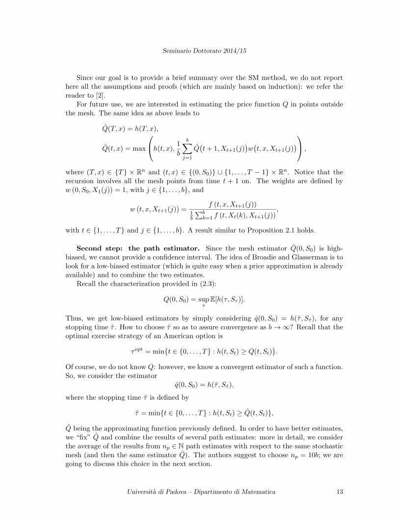
Since our goal is to provide a brief summary over the SM method, we do not reporthere all the assumptions and proofs (which are mainly based on induction): we refer thereader to [2].
For future use, we are interested in estimating the price function Q in points outsidethe mesh. The same idea as above leads to
Q(T, x) = h(T, x),
Q(t, x) = max
h(t, x),1
b
b∑j=1
Q(t+ 1, Xt+1(j)
)w(t, x,Xt+1(j)
) ,
where (T, x) ∈ T × Rn and (t, x) ∈ (0, S0) ∪ 1, . . . , T − 1 × Rn. Notice that therecursion involves all the mesh points from time t + 1 on. The weights are defined byw (0, S0, X1(j)) = 1, with j ∈ 1, . . . , b, and
w (t, x,Xt+1(j)) =f (t, x,Xt+1(j))
1b
∑bk=1 f (t,Xt(k), Xt+1(j))
,
with t ∈ 1, . . . , T and j ∈ 1, . . . , b. A result similar to Proposition 2.1 holds.
Second step: the path estimator. Since the mesh estimator Q(0, S0) is high-biased, we cannot provide a confidence interval. The idea of Broadie and Glasserman is tolook for a low-biased estimator (which is quite easy when a price approximation is alreadyavailable) and to combine the two estimates.
Recall the characterization provided in (2.3):
Q(0, S0) = supτ
E[h(τ, Sτ )].
Thus, we get low-biased estimators by simply considering q(0, S0) = h(τ , Sτ ), for anystopping time τ . How to choose τ so as to assure convergence as b→∞? Recall that theoptimal exercise strategy of an American option is
τopt = mint ∈ 0, . . . , T : h(t, St) ≥ Q(t, St).
Of course, we do not know Q: however, we know a convergent estimator of such a function.So, we consider the estimator
q(0, S0) = h(τ , Sτ ),
where the stopping time τ is defined by
τ = mint ∈ 0, . . . , T : h(t, St) ≥ Q(t, St),
Q being the approximating function previously defined. In order to have better estimates,we “fix” Q and combine the results of several path estimates: more in detail, we considerthe average of the results from np ∈ N path estimates with respect to the same stochasticmesh (and then the same estimator Q). The authors suggest to choose np = 10b; we aregoing to discuss this choice in the next section.
Universita di Padova – Dipartimento di Matematica 13
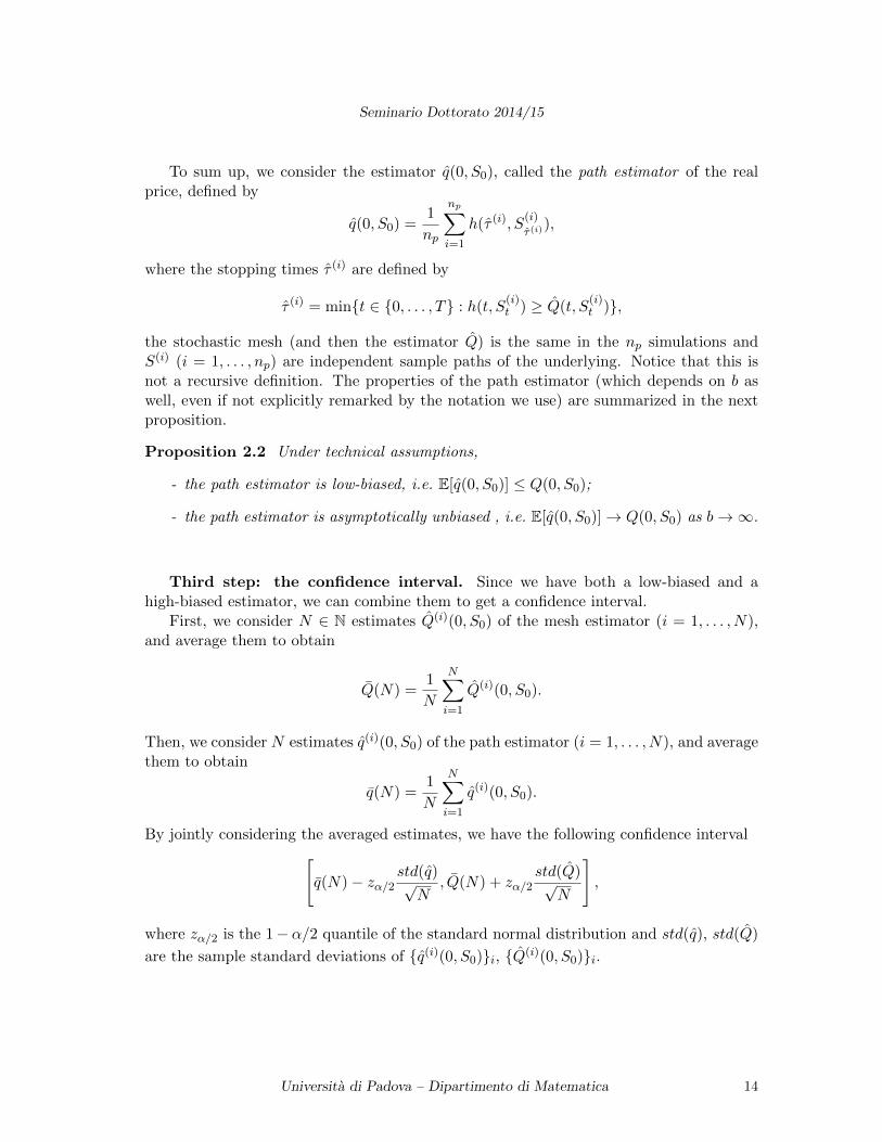
Seminario Dottorato 2014/15
To sum up, we consider the estimator q(0, S0), called the path estimator of the realprice, defined by
q(0, S0) =1
np
np∑i=1
h(τ (i), S(i)
τ (i)),
where the stopping times τ (i) are defined by
τ (i) = mint ∈ 0, . . . , T : h(t, S(i)t ) ≥ Q(t, S
(i)t ),
the stochastic mesh (and then the estimator Q) is the same in the np simulations andS(i) (i = 1, . . . , np) are independent sample paths of the underlying. Notice that this isnot a recursive definition. The properties of the path estimator (which depends on b aswell, even if not explicitly remarked by the notation we use) are summarized in the nextproposition.
Proposition 2.2 Under technical assumptions,
- the path estimator is low-biased, i.e. E[q(0, S0)] ≤ Q(0, S0);
- the path estimator is asymptotically unbiased , i.e. E[q(0, S0)]→ Q(0, S0) as b→∞.
Third step: the confidence interval. Since we have both a low-biased and ahigh-biased estimator, we can combine them to get a confidence interval.
First, we consider N ∈ N estimates Q(i)(0, S0) of the mesh estimator (i = 1, . . . , N),and average them to obtain
Q(N) =1
N
N∑i=1
Q(i)(0, S0).
Then, we consider N estimates q(i)(0, S0) of the path estimator (i = 1, . . . , N), and averagethem to obtain
q(N) =1
N
N∑i=1
q(i)(0, S0).
By jointly considering the averaged estimates, we have the following confidence interval[q(N)− zα/2
std(q)√N
, Q(N) + zα/2std(Q)√
N
],
where zα/2 is the 1−α/2 quantile of the standard normal distribution and std(q), std(Q)
are the sample standard deviations of q(i)(0, S0)i, Q(i)(0, S0)i.
Universita di Padova – Dipartimento di Matematica 14
Seminario Dottorato 2014/15
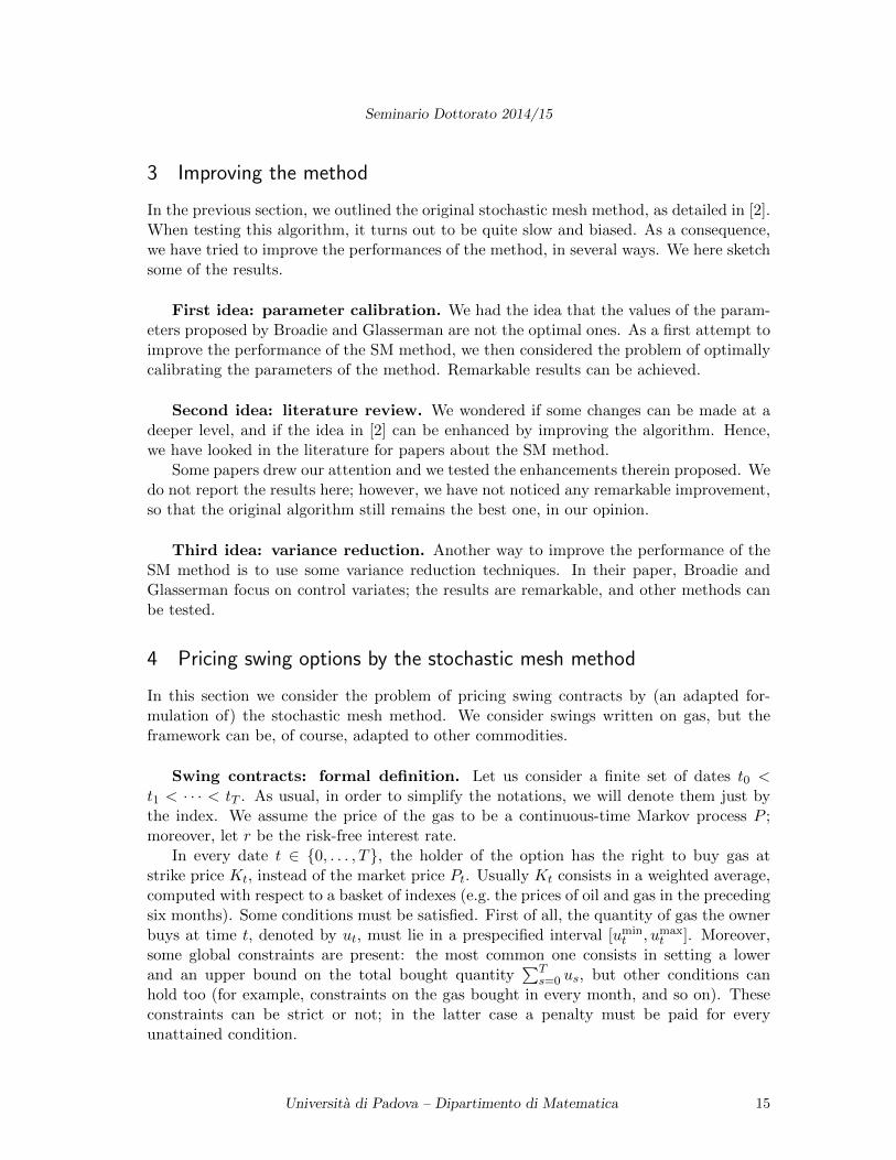
3 Improving the method
In the previous section, we outlined the original stochastic mesh method, as detailed in [2].When testing this algorithm, it turns out to be quite slow and biased. As a consequence,we have tried to improve the performances of the method, in several ways. We here sketchsome of the results.
First idea: parameter calibration. We had the idea that the values of the param-eters proposed by Broadie and Glasserman are not the optimal ones. As a first attempt toimprove the performance of the SM method, we then considered the problem of optimallycalibrating the parameters of the method. Remarkable results can be achieved.
Second idea: literature review. We wondered if some changes can be made at adeeper level, and if the idea in [2] can be enhanced by improving the algorithm. Hence,we have looked in the literature for papers about the SM method.
Some papers drew our attention and we tested the enhancements therein proposed. Wedo not report the results here; however, we have not noticed any remarkable improvement,so that the original algorithm still remains the best one, in our opinion.
Third idea: variance reduction. Another way to improve the performance of theSM method is to use some variance reduction techniques. In their paper, Broadie andGlasserman focus on control variates; the results are remarkable, and other methods canbe tested.
4 Pricing swing options by the stochastic mesh method
In this section we consider the problem of pricing swing contracts by (an adapted for-mulation of) the stochastic mesh method. We consider swings written on gas, but theframework can be, of course, adapted to other commodities.
Swing contracts: formal definition. Let us consider a finite set of dates t0 <t1 < · · · < tT . As usual, in order to simplify the notations, we will denote them just bythe index. We assume the price of the gas to be a continuous-time Markov process P ;moreover, let r be the risk-free interest rate.
In every date t ∈ 0, . . . , T, the holder of the option has the right to buy gas atstrike price Kt, instead of the market price Pt. Usually Kt consists in a weighted average,computed with respect to a basket of indexes (e.g. the prices of oil and gas in the precedingsix months). Some conditions must be satisfied. First of all, the quantity of gas the ownerbuys at time t, denoted by ut, must lie in a prespecified interval [umin
t , umaxt ]. Moreover,
some global constraints are present: the most common one consists in setting a lowerand an upper bound on the total bought quantity
∑Ts=0 us, but other conditions can
hold too (for example, constraints on the gas bought in every month, and so on). Theseconstraints can be strict or not; in the latter case a penalty must be paid for everyunattained condition.
Universita di Padova – Dipartimento di Matematica 15
Seminario Dottorato 2014/15
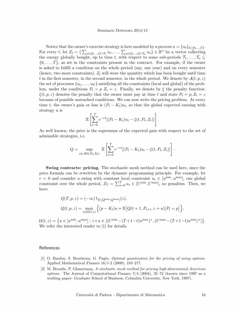
Notice that the owner’s exercise strategy is here modeled by a process u = utt∈0,...,T.For every t, let Zt =
(∑s∈0,...,t∩T1 us, . . . ,
∑s∈0,...,t∩Tn us
)∈ Rn be a vector collecting
the energy globally bought, up to time t, with respect to some sub-periods T1, . . . , Tn ⊆0, . . . , T, as set in the constraints present in the contract. For example, if the owneris asked to fulfill a condition on the whole period (say, one year) and on every semester(hence, two more constraints), Zt will store the quantity which has been bought until timet in the first semester, in the second semester, in the whole period. We denote by A(t, p, z)the set of processes ut, . . . , uT satisfying all the constraints (local and global) of the prob-lem, under the conditions Pt = p Zt = z. Finally, we denote by ξ the penalty function:ξ(t, p, z) denotes the penalty that the owner must pay at time t and state Pt = p, Zt = zbecause of possible unreached conditions. We can now write the pricing problem. At everytime t, the owner’s gain or loss is (Pt −Kt)ut, so that the global expected earning withstrategy u is
E
[T∑t=0
e−rt[(Pt −Kt)ut − ξ(t, Pt, Zt)]
].
As well known, the price is the supremum of the expected gain with respect to the set ofadmissible strategies, i.e.
Q = supu∈A(0,P0,Z0)
E
[T∑t=0
e−rt[(Pt −Kt)ut − ξ(t, Pt, Zt)]
].
Swing contracts: pricing. The stochastic mesh method can be used here, since theprice formula can be rewritten by the dynamic programming principle. For example, letr = 0 and consider a swing with constant local constraint ut ∈ [umin, umax], one globalconstraint over the whole period, ZT =
∑Ts=0 us ∈ [Umin, Umax], no penalties. Then, we
have
Q(T, p, z) = (−∞)1R\[Qmin,Qmax](z),
Q(t, p, z) = maxu∈U(t,z)
(p−Kt)u+ E
[Q(t+ 1, Pt+1, z + u)
∣∣Pt = p],
U(t, z) =u ∈ [umin, umax] : z+u ∈ [(Umin−(T+1−t)umax)+, (Umax−(T+1−t)umin)+]
.
We refer the interested reader to [1] for details.
References
[1] O. Bardou, S. Bouthemy, G. Pages, Optimal quantization for the pricing of swing options.Applied Mathematical Finance 16/1-2 (2009), 183–217.
[2] M. Broadie, P. Glasserman, A stochastic mesh method for pricing high-dimensional Americanoptions. The Journal of Computational Finance 7/4 (2004), 35–72 (known since 1997 as aworking paper: Graduate School of Business, Columbia University, New York, 1997).
Universita di Padova – Dipartimento di Matematica 16
Seminario Dottorato 2014/15
[3] M. Broadie, P. Glasserman, Pricing American-style securities by simulation. Journal of Eco-nomic Dynamics and Control 21 (1997), 1323–1352.
[4] P. Glasserman, “Monte Carlo Methods in Financial Engineering”. Springer-Verlag, New York,2004.
[5] F. A. Longstaff, E. S. Schwartz, Valuing American options by simulation: a simple least-squaresapproach. Review of Financial Studies 14 (2001), 113–147.
Universita di Padova – Dipartimento di Matematica 17
Seminario Dottorato 2014/15
Singular perturbations of stochastic control
problems with unbounded fast variables
Joao Meireles (∗)
Abstract. In this talk, we first give a short introduction to singular perturbations problems andto the Hamilton-Jacobi approach to the singular limit ε → 0. Then, we consider a specific singu-lar perturbation problem of a class of optimal stochastic control problems with unbounded andcontrolled fast variables and we discuss (briefly) how to solve it.
1 Statement of the problem
In a classic singular perturbed system (SPS) the state variables evolve along two differenttime scales: a positive parameter ε appears in front of one of the time derivatives affectingits velocity - the equation of the fast variables. Our problem is to describe and understandthe asymptotic behaviour of a (SPS) as the parameter ε vanishes.
A simple model is
(Sε)
x(t) = f(x(t), y(t), a(t)), x(0) = xεy(t) = g(x(t), y(t), a(t)), y(0) = y
where
• x ∈ Rn and y belongs to Tm ' Rm/Zm (the flat torus);
• the functions a(·) are controls and they are measurable functions from [0,∞) to acompact metric space A (and we will denote by A the set of all these functions);
• f and g are continuous functions in all their variables and Lipchitz-continuous in(x, y) uniformly with respect to the control a.
(Sε) is a good example of a singular perturbed control system. As mentioned before, therole of ε is obvious: it splits the state variables in two groups, one, a group of n slow
(∗)Ph.D. course, Universita di Padova, Dip. Matematica, via Trieste 63, I-35121 Padova, Italy; E-mail:. Seminar held on November 19th, 2014.
Universita di Padova – Dipartimento di Matematica 18
Seminario Dottorato 2014/15
variables evolving in a macroscopic time scale, and, another, a group of m fast variablesevolving along a microscopic time scale. This is the reason why the study of multiscaleproblems is an important issue in many applications of engineering, chemistry and physics.Many phenomena can be modelled by a (SPS).
Here we are interested in characterising and analysing the asymptotic behaviour of (Sε) asε → 0 (if this makes sense). It is expected that passing to the limit as ε → 0+ in the theinitial problem amounts to reducing the dimension of the state space and that the limitdynamics (S) (if it exists) involves only the slow variables.
2 Some approaches to singular perturbations problems
There are some approaches to address our problem. Here we present the most relevantones:
• (The Levinson-Tikhonov method) This approach consists in considering, as the nat-ural candidate for the limit, the system obtained by setting ε = 0 in (Sε). The resultis an ordinary differential equation combined with an algebraic equation. This ap-proach gives the appropriate solution when the stationary points of the fast dynamicsare attractive, a condition that may fail to be satisfied.
• (Limit of occupational measures) Other averaging approaches have been proposedby Artstein in the context of invariant measure theory (see [5]), and by Gaitsgoryand Leizarowitz, using limit occupational measures (see [11]).
• A PDE method based in the theory of viscosity solutions and of the homogenisationof fully nonlinear PDEs was developed by Alvarez and Bardi in [1,2,3], also [4] forproblems with an arbitrary number of scales. This the approach that we will considerin this note.
3 The PDE approach to singular perturbations problems
It is well known that under some regularity conditions the value function V ε of (Sε), i.e,
V ε(t, x, y) := infl(x(s), y(s), a(s))ds+ h(x(s), y(s)),
where l and h are given functions and the inf is being taken among all admissible controls,satisfies the Hamilton-Jacobi-Bellman equation
(1) (HJB)ε
V εt +H
(x, y,DxV
ε,DyV ε
ε
)= 0
V ε(0, x, y) = h(x, y)
where DxVε, DyV
ε stand for the gradient of V ε with respect to x and y respectively, and
Universita di Padova – Dipartimento di Matematica 19
Seminario Dottorato 2014/15
H is the Hamilton-Jacobi-Bellman operator
H(x, y, p, q) := maxa∈A−p · f(x, y, a)− q · g(x, y, a)− l(x, y, a).
The PDE approach to (SPP) consists in passing to the limit in the PDE (HJB)ε. Undersuitable conditions, it is possible to define an effective Hamiltonian H(x, p) such that theV ε converges locally uniformly, as ε→ 0, to a solution of
(2)
Vt + H(x,DxV ) = 0V (0, x, y) = h(x).
The proof of the existence of such an operator H, and the analysis of some of its properties,embody a wide line of research, going back to the first works on homogenisation of PDEs(see for example [10]) and, in particular, to the famous unpublished preprint [16] by Lions,Papanicolaou and Varadhan.
In the paper [2], two crucial properties about the convergence of the V ε has been singledout by the authors. One is an ergodicity property of the operator H, and therefore H, andanother is a property called stabilization to a constant of the pair (H,h) that allows thepossibility to define the effective initial datum h for the effective Cauchy problem (2). Allthese properties permit to establish the uniform convergence of V ε to the solution of theeffective equation and in some cases to prove that the effective Hamiltonian is the partialdifferential operator associated to the limit control problem (S). However, this theory wasdeveloped mostly for fast variables restricted to a compact set (almost all in the case ofthe m-dimensional torus). Nonetheless, in many physical and financial models the a prioriknowledge of the boundedness of the fast variables does not appear to be natural accordingto the empirical data. Very few has been done until now to treat the unboundedness case.
In the papers [7] and [8] the authors present an extension of the methods based on vis-cosity solutions showed in [1, 2, 3] to singular perturbation problems that have unboundedbut uncontrolled fast variables.
4 Singular perturbations with unbounded fast variables
In my thesis, I study singular perturbations of a class of optimal stochastic control prob-lems with finite time horizon and with unbounded and uncontrolled fast variables. Theproblem I treat is for t ∈ [0, T ] and given θ∗ > 1 and ε > 0
minimize in u and ξ: Ex,y[∫ Tt (l(Xs, Ys, us) + 1
θ∗ |ξs|θ∗)ds+ g(XT )]
subject to
(3)
dXs = F (Xs, Ys, us)ds+
√2σ(Xs, Ys, us)dWs, Xs0 = x
dYs = −1ε ξsds+
√1ε τ(Ys)dWs, Ys0 = y
Universita di Padova – Dipartimento di Matematica 20
Seminario Dottorato 2014/15
where l is a running cost function satisfying the following coercivity condition
−l0 + l−10 |y|
α ≤ l(x, y, u) ≤ l0(1 + |y|α) for some l0 > 0
where α > 1, g represents a terminal cost and is continuous, bounded from below, andgrowing like
∃Cg > 0 s.t. g(x) ≤ Cg(1 + |x|α),
and Xs ∈ Rn, Ys ∈ Rm, us is a control taking values in a given compact set U , ξ =(ξs)0≤s≤T denotes a control process taking its values in Rm, and Ws is a multi-dimensionalBrownian motion on some probability space.
Basic assumptions on the drift F and on the diffusion coefficient σ of the slow variablesXs are that they are Lipschitz continuos functions in (x, y) uniformly in u and satisfy thefollowing growth condition at infinity
|F |+ ||σ|| ≤ C(1 + |x|).
On the fast process Ys we assume that ττT = I.
Calling V ε(t, x, y) the value function of this optimal control problem, i.e.
V ε(t, x, y) = infu,ξ
Ex,y[∫ T
t(l(Xs, Ys, us) +
1
θ∗|ξs|θ
∗)ds+ g(XT )],
we are interested in the limit V as ε → 0 of V ε and in particular in understanding thePDE satisfied by V . This is a singular perturbation problem for the system above and forthe HJB equation associated to it. We treat it by PDE methods and a careful analysis ofthe associated ergodic stochastic control problem in the whole space Rm.
In fact, in Theorem 10.1 (see [17]) I prove that if V ε(t, x, y) is a viscosity solution ofthe HJB equation then the relaxed semilimits (no standard ones!)
(4) V (t, x) = lim inf(ε,t′,x′)→(0,t,x)
infy∈Rm
V ε(t′, x′, y)
and
(5) V = (supRVR)∗
(the upper semicontinuous envelope of supR VR) where VR is defined as
(6) VR(t, x) = lim sup(ε,t′,x′)→(0,t,x)
supy∈BR(0)
V ε(t′, x′, y)
are, respectively, a supersolution and a subsolution of the effective Cauchy Problem
(7)
−Vt + H(x,DxV,D
2xxV ) = 0 in (0,∞)× Rn
V (T, x) = g(x) in Rn.
Universita di Padova – Dipartimento di Matematica 21
Seminario Dottorato 2014/15
This procedure allow me to prove also that in some cases V ε(t, x, y) converges locallyuniformly, as ε→ 0, to the only solution V (t, x) of (7). Moreover, the effective HamiltonianH(x, p,M) is the unique constant λ such that the following ergodic PDE
(EP ) λ− 1
2∆φ(y) +
1
θ|Dφ(y)|θ = f(y) in Rm,
has a solution φ bounded from below, 1θ + 1
θ∗ = 1 and f(y) = −H(x, y, p,M, 0), whereH is the Bellman Hamiltonian associated to the slow variables of (3) and its last entryis for the mixed derivatives Dxy. Such type of equations appear in utility maximisationproblems in mathematical finance and were first studied by Naoyuki Ichihara in [Ichihara,2012] using probabilistic and analytical arguments.
References
[1] O. Alvarez, M. Bardi, Viscosity solutions methods for singular perturbations in deterministicand stochastic control. SIAM J. Control Optim. 40 (2001/02), 1159–1188.
[2] O. Alvarez, M. Bardi, Singular perturbations of nonlinear degenerate parabolic PDEs: a generalconvergence result. Arch. Ration. Mech. Anal. 170 (2003), 17–61.
[3] O. Alvarez, M. Bardi, Ergodicity, stabilisation, and singular perturbations for Bellman-Isaacsequations. Mem. Amer. Math. Soc. (2010).
[4] O. Alvarez, M. Bardi, C. Marchi, Multiscale problems and homogenisation for second-orderHamilton-Jacobi equations. J. Differential Equations 243 (2007), 349–387.
[5] Z. Artstein, Stability in presence of singular perturbations. Nonlinear Analysis 33 (1998),817–827.
[6] M. Bardi, I. Capuzzo Dolcetta, “Optimal control and viscosity solutions of Hamilton-Jacobi-Bellman equations”. Birkauser, Boston, 1997.
[7] M. Bardi, A. Cesaroni, Optimal control with random parameters: a multiscale approach. J.Control 17/1 (2011), 30–45.
[8] M. Bardi, A. Cesaroni, L. Manca, Convergence by viscosity methods in multiscale financialmodels with stochastic volatility. SIAM J. Financial Math. 1 (2010), 230–265.
[9] V. S. Borkar, V. Gaitsgory, Singular perturbations in ergodic control of diffusions. SIAM J.Control Optim. 46 (2007), 1562–1577.
[10] L. C. Evans, The perturbed test function method for viscosity solutions of nonlinear PDE. Proc.Roy. Soc. Edinburgh Sect. A 111 (1989), 359–375.
[11] V. Gaitsgory, A. Leizarowitz, Limit Occupational Measures Set for a Control System andAveraging of Singularly Perturbed Control System. Journal of Mathematical Analysis andApplications 233 (1999), 461–475.
[12] N. Ichihara, Recurrence and transience of optimal feedback processes associated with Bellmanequations of ergodic type. SIAM J. Control Optim. 49/5 (2011), 1938–1960.
Universita di Padova – Dipartimento di Matematica 22
Seminario Dottorato 2014/15
[13] N. Ichihara, Large time asymptotic problems for optimal stochastic control with super linearcost. Stochastic Processes and their Applications 122 (2012), 1248–1275.
[14] N. Ichihara and S.-J. Sheu, Large time behaviour of solutions of Hamilton-Jacobi-Bellmanequations with quadratic nonlinearity in gradients. SIAM J. Math. Anal. 45/1 (2013), 279–306.
[15] P. Kokotovic, H. Khalil, J. O’Reilly, “Singular Perturbation Methods in Control: Analysisand Design”. Academic Press, London, 1986.
[16] P.-L. Lions, G. Papanicolaou, S. R. S. Varadhan, Homogenisation of Hamilton-Jacobi equa-tions. Unpublished (1986).
[17] J. Meireles, “Singular Perturbations and Ergodic Problems for degenerate parabolic BellmanPDEs in Rm with Unbounded Data”. Phd thesis. Universita degli Studi di Padova, 2015.
Universita di Padova – Dipartimento di Matematica 23
Seminario Dottorato 2014/15
An introduction to density
estimates for diffusion processes
Paolo Pigato (∗)
Abstract. We recall some notions in Malliavin calculus and some general criteria for the absolutecontinuity and regularity of the density of a diffusion. We present some estimates for degeneratediffusion processes under a weak Hormander condition, obtained starting from the Malliavin andThalmaier representation formula for the density. As an example, we focus in particular on thestochastic differential equation used to price Asian Options.
1 Elements of Malliavin Calculus
Malliavin calculus is an infinite-dimensional differential calculus on the Wiener space. It isuseful to investigate regularity properties of solutions of stochastic differential equations,and its most important application is a probabilistic proof of Hormander’s theorem.
A crucial fact in this theory is the integration-by-parts formula, which relates thederivative operator on the Wiener space and the Skorohod extended stochastic integral.A consequence of this is a formula which links existence and regularity of the density of arandom variable to the so-called ”Malliavin covariance matrix”.
We introduce some basic notions, referring to [8]. We consider a probability space(Ω,F , P ), a Brownian motion W = (W 1
t , ...,Wdt )t≥0 and the filtration (Ft)t≥0 generated
by W . For fixed T > 0, we denote with H the Hilbert space L2([0, T ],Rd). For h ∈ H we
introduce this notation for the Ito integral of h: W (h) =∑d
j=1
∫ T0 hj(s)dW j
s . We denoteby C∞p (Rn) the set of all infinitely continuously differentiable functions f : Rn → R suchthat f and all of its partial derivatives have polynomial growth. We also denote by S theclass of random variables of the form
F = f(W (h1), ...,W (hn)),
for some f ∈ C∞p (Rn), h1, ..., hn in H, n ≥ 1. The Malliavin derivative of F ∈ S is defined
(∗)Ph.D. course, Universita di Padova, Dip. Matematica, via Trieste 63, I-35121 Padova, Italy; E-mail:. Seminar held on November 26th, 2014.
Universita di Padova – Dipartimento di Matematica 24
Seminario Dottorato 2014/15
as the H valued random variable given by
DF =n∑i=1
∂f
∂xi(W (h1), ...,W (hn))hi.
Remark that this implies D∫ T
0 hi(s)dWs = hi. Therefore, this expression can be seen asthe germ of a chain-rule formula and is therefore a reasonable definition for a ”derivative”.
The extension of the definition of D on a wider domain requires the introduction ofthe Sobolev norm of F :
‖F‖1,p = [E|F |p + ‖DF‖pH ]1p where ‖DF‖H =
(∫ T
0|DsF |2ds
) 12
.
It is possible to prove that D is a closable operator with respect to this norm an take theextension of D in the standard way. We can now define in the obvious way DF for anyF in the closure of S with respect to this norm. Therefore, the domain of D will be theclosure of S.
The higher order derivative of F is obtained by iteration. For any k ∈ N, for a multi-index α = (α1, ..., αk) ∈ 1, ..., dk and (s1, ..., sk) ∈ [0, T ]k, we can define
Dαs1,...,sk
F := Dα1s1 ...D
αkskF.
We denote with |α| = k the length of the multi-index. Remark that Dαs1,...,sk
F , is a random
variable with values in H⊗k, and its Sobolev norm is defined as
‖F‖k,p = [E|F |p +k∑j=1
|D(j)F |p]1p
where
|D(j)F |2 =
∑|α|=j
∫[0,T ]k
|Dαs1,...,sk
F |2ds1...dsk
1/2
.
The extension to the closure of S with respect to this norm is analogous to the firstorder derivative. We denote by Dk,p the space of the random variables which are k timesdifferentiable in the Malliavin sense in Lp, and Dk,∞ =
⋂∞p=1 Dk,p.
We denote with δ the adjoint operator of D, the so-called Skorohod integral. It ispossible to prove that δ coincides with the Ito integral for adapted integrands, and thatthe following formula holds, for any F ∈ D1,2 and u ∈ Dom(δ) such that F ∈ L2(Ω,H):
(1) δ(Fu) = Fδ(u)− E〈DF, u〉H .
We consider a random vector F = (F1, ..., Fn) in the domain of D. We define its Malliavincovariance matrix as follows:
γi,jF = 〈DFi, DFj〉H =d∑
k=1
∫ T
0DksFi ×Dk
sFjds.
Universita di Padova – Dipartimento di Matematica 25
Seminario Dottorato 2014/15
We say that F is non-degenerate if its Malliavin covariance matrix is invertible and
(2) E(|det γF |−p) <∞, ∀p ∈ N.
We denote with γF the inverse of γF . Using (1) it is possible to prove the followingintegration by parts formula. Let F ∈ D2,2 be a scalar r.v. such that (2) holds. Then forevery G ∈ D2,2
(3) E[φ′(F )G] = E[φ(F )H(F ;G)], ∀φ ∈ C∞c (R)
where the Malliavin weights are given by
H(F ;G) = −GγF × LF + 〈D(γFG), DF 〉.
Here L = −δ D is the Ornstein-Uhlenbeck operator. This integration by parts formula isreally important, because if it holds it tells us that F is absolutely continuous with respectto the Lebesgue measure and allows us to write this representation for the density:
pF (x) = E[1[x,∞)(F )H(F ; 1)].
The intuition behind this fact is the following: we first express the density as pF (x) =E[δ0(F − x)]. Then we formally write the Dirac delta in 0 as δ0(y) = ∂y1[0,∞)(y), andapply (3)
E[δ0(F − x)] = E[∂1[0,∞)(F − x)] = E[1[x,∞)(F )H(F, 1)].
If higher order integration by parts formula are available, they can be employed to findanalogous expressions for the derivatives of the density, iterating the procedure above.
The following multidimensional generalisation has been proved by Malliavin and Thal-maier in [7]:
pF (x) = −E [∇Qn(F − x)H(F ; 1)] ,
where Qn denotes the Poisson kernel on Rn, i.e. the fundamental solution of the Laplaceoperator ∆Qn = δ0. This is given by
Q1(x) = max(x, 0); Q2(x) = A−12 ln |x|; Qn(x) = −A−1
n |x|2−n, n > 2,
where An is the area of the unit sphere in Rn.
2 Application to diffusion processes
2.1 Hormander theorem
The original motivation and the most important application of the integration by partsmentioned in the previous section is a probabilistic proof of the Hormander theorem.
Let Xt, t ∈ [0, T ] be the solution of the following stochastic differential equation in Rn:
X0 = x, dXt =
d∑i=1
σi(Xt)dWit + b(Xt)dt,
Universita di Padova – Dipartimento di Matematica 26
Seminario Dottorato 2014/15
with W = (W 1, . . . ,W d) ∈ Rd, X ∈ Rn. We assume infinitely differentiable coefficientswith bounded partial derivatives of all orders. We denote σ0 = b.
For f, g : Rn → Rn we recall the definition of the directional derivative of f in thedirection g as
∂gf(x) =
n∑i=1
gi(x)∂xif(x).
The Lie bracket [f, g] in x is defined as
[f, g](x) = ∂gf(x)− ∂fg(x).
We say that the Hormander condition holds at point x if the vector space spanned by thevector fields
σ1, . . . , σd, [σi, σj ], 0 ≤ i, j ≤ d, [σi, [σj , σk]], 0 ≤ i, j, k ≤ d, . . .
at x is Rn.
Theorem 1 Assume that the Hormander condition holds at the initial point x. Then fort ∈ [0, T ] the random vector Xt has a probability distribution that is absolutely continuouswith respect to the Lebesgue measure, and the density is infinitely differentiable.
This result can be viewed as a probabilistic version of Hormander’s theorem on thehypoellipticity of second-order differential operators. We refer to [8] for details. The proofrelies on the fact that Xt is non-degenerate (meaning that (2) holds for F = Xt) for anyt > 0, if the Hormander condition at x is satisfied.
Remark 2 A similar theorem applies for the density pXt(y) at y if the Hormandercondition holds at y.
2.2 Bounds for the density
If it exists, define pt(x, y) as the density of Xt in y, with initial condition in x. Malliavincalculus also allows to find quantitative estimates for pt(x, y). We expect these estimatesto be Gaussian, since the SDE satisfied by Xt is a diffusion driven by a Brownian motion.
We now look closer at the Hormander non-degeneracy assumption. We say that theStrong Hormander condition holds at x if the vector space spanned by the vector fields
σ1, . . . , σd, [σi, σj ], 1 ≤ i, j ≤ d, [σi, [σj , σk]], 1 ≤ i, j, k ≤ d, . . .
at x is Rn. On the other hand, we say that the Weak Hormander condition at x holds ifthe vector space spanned by the vector fields
σ1, . . . , σd, [σi, σj ], 0 ≤ i, j ≤ d, [σi, [σj , σk]], 0 ≤ i, j, k ≤ d, . . .
at x is Rn (recall σ0 is the drift term). Also recall that we say that our diffusion is ellipticif the vector space spanned by the vector fields σ1, . . . , σd is Rn. Estimates of the densityare well known under this assumption, but it is a quite demanding one. For instance,
Universita di Padova – Dipartimento di Matematica 27
Seminario Dottorato 2014/15
ellipticity implies n ≤ d, i.e. the dimension of the driving Brownian Motion must be atleast the same as the dimension of the diffusion itself. This is not true if we just supposethe strong Hormander condition. Indeed, we can use the brackets [σi, σj ], 1 ≤ i, j ≤ d andtheir iterations to span Rn. Weak Hormander condition allows us to use also the bracketsbetween diffusion and drift coefficients, and therefore it is the weakest of the three. Wehave seen in the previous section that this condition is sufficient to prove existence andregularity of the density. But is it enough to find some Gaussian bounds?
The most celebrated work on this topic is a series of three papers by Kusuoka andStroock in the the eighties. In [5] the authors prove, under the weak Hormander condition,the following upper bounds:
pt(x, y) ≤ C0(T )(1 + |x|)m0
tn0exp
(−D0(T )|y − x|2
t
)Dαy pt(x, y) ≤ Cα(T )(1 + |x|)mα
tnαexp
(−Dα(T )|y − x|2
t
)where all the above constants depend on how many iterated Lie brackets we have to taketo span Rn, and on the final time T . Here Dα
y denotes the derivative of order α of pt(x, y)with respect to y. Lower bounds of this kind, in general, are not available.
Two-sided bounds in terms of a control metric are established in [6] under strongHormander conditions if the drift is generated by the vector fields of the diffusive part.The standard control metric is defined as follows. For x, y ∈ Rn we denote by C(x, y) theset of controls ψ ∈ L2([0, 1];Rn) such that the corresponding skeleton (ut)t∈[0,1] solutionof
dut(ψ) =
d∑j=1
σj(ut(ψ))ψjt dt, u0(ψ) = x
satisfies u1(ψ) = y. Notice that the drift b = σ0 does not appear in the equation of ut(ψ).We define the control (Caratheodory) distance as
dc(x, y) = inf(∫ 1
0|ψs|2 ds
)1/2: ψ ∈ C(x, y)
.
These metrics are really important in various fields of mathematics, having fundamentalrole in particular in sub-Riemannian geometry. The following estimates are proved: thereexist a constant M ≥ 1 such that
1
M |Bd(x, t1/2)|exp
(−Md(x, y)2
t
)≤ pt(x, y) ≤ M
|Bd(x, t1/2)|exp
(−d(x, y)2
Mt
)(4)
for (t, x, y) ∈ (0, 1]× Rn × Rn, where Bd(x, r) = y ∈ Rn : d(x, y) < r.
Remark 3 As we said before, this estimate holds if the drift is generated by the vectorfields of the diffusive part, meaning b =
∑k=1d αkσk, for some α1, . . . , αd ∈ C∞b (Rn). This
is a slight generalisation of the pure-diffusion case b = 0.
Universita di Padova – Dipartimento di Matematica 28
Seminario Dottorato 2014/15
3 A diffusion process under a weak Hormander condition
In this last section we present some original result, based on [9]. We consider a diffusionprocess
(5) Xt = x+
∫ t
0σ(Xs) dWs +
∫ t
0b(Xs)ds,
where X is in dimension two, W is in dimension one, and dWs denotes the Stratonovichintegral. This clearly implies that our diffusion cannot be elliptic, but it also implies thatthe strong Hormander condition cannot be satisfied, since σ is just a column vector. Ournon-degeneracy assumption is indeed of weak Hormander type: we suppose that σ and[b, σ] span R2, and we suppose it just locally, in a sense that we will specify later. We arein a different framework respect to the classical result (4) (cf. Remark 3), since here wedo not just allow a drift, but we actually need it to have the non-degeneracy. It is thanksto the existence of the drift that the randomness spreads in all directions and not just inthe direction of σ. There has been some interest in recent years in density estimates forsimilar weak-Hormander type models, see for instance [2] and [1].
The prototype of this kind of problems is a two dimensional system where the firstcomponent X1 follows a stochastic dynamic, and the second component X2 is a determin-istic functional of X1, so the randomness acts indirectly on X2. A natural application isthe equation used price the Asian option:
X1t = x1 +
∫ t
0σ1(X1
s ) dWs +
∫ t
0b1(X1
s )ds, X2t =
∫ t
0b2(X1
s )ds.
Here X1 represents the price of a stock following a local volatility model. X2 is an averageof the underlying price over some pre-set period of time, which determines the payoff ofthe so-called Asian options on X1. In this case it is easy to see that σ and [b, σ] span R2
if and only if σ1∂b2 6= 0. This is what one would expect, since the randomness should acton X1, and X2 should see it through a dependence on X1.
There are other possible application, such as in [3], [4]. These papers deal with astochastic Hodgkin-Huxley model for the functioning of a neuron: X2 is the concentrationof some chemicals resulting from a reaction involving the first component X1. Differentlyfrom our setting, though, there are several measurements corresponding to the input X1,so X2 is multi-dimensional. The pattern, however, is similar.
We take a control φ ∈ L2[0, T ], and the associated skeleton path solution of
(6) xt(φ) = x+
∫ t
0σ(xs(φ))φsds+
∫ t
0b(xs(φ))ds.
We are interested in a tube estimate for (5), which is still an open problem under thisweak non-degeneracy assumption. With tube estimate we mean that we are interested inP(supt≤T ‖Xt − xt(φ)‖ ≤ R
). Several works have considered this subject, starting from
Stroock and Varadhan in [10]. For them ‖ · ‖ is the Euclidean norm, but later on differentnorms have been used to take into account the regularity of the trajectories. This is
Universita di Padova – Dipartimento di Matematica 29
Seminario Dottorato 2014/15
somehow true also in our case. Indeed, because of the weak Hormander framework, ourdiffusion is non-isotropic. This means that it moves with different speeds in differentdirections. More precisely, it moves with speed t1/2 in the direction σ and t3/2 in thedirection [b, σ]. To account of this fact, we have to introduce a suitable norm. For anyR > 0, we denote with AR(x) the matrix
(R1/2σ(x), R3/2[b, σ](x)
). For fixed R, since we
suppose the weak Hormander condition and AR(x) is invertible, we associate to AR(x)the norm
|ξ|AR(x) =√〈(AR(x)AR(x)T )−1ξ, ξ〉 = |A−1
R (x)ξ|
on Rn. This is what we need, because it allows us to weight the two time scales in theappropriate way. Let us have a closer look at this norm for the Asian option SDE, i.e.σ2(x) = 0:
AR(x) =(R1/2σ(x), R3/2[b, σ](x)
)=
(σ1(x1)R1/2 (. . . )R3/2
0 σ1∂b(x1)R3/2
).
In this case the associated norm is equivalent to |ξ|∗ = |(R−1/2ξ1, R−3/2ξ2)|. Here it iseasier to see what is going on. The first component, following a diffusive dynamic, mustbe weighted according to the time scale t1/2. The second component, which is integratedin time once more, must be weighted according to the time scale t1/2×t = t3/2. Analogousnorms appear, in a multidimensional framework, in [2]. Just remark that the results thatwe are going to state here hold for a more general model in the sense that we allow σ2 6= 0.
We suppose σ, b differentiable three times, denote l(x) the smallest eigenvalue ofA(x) = (σ, [b, σ])(x), and n(x) =
∑3k=0
∑|α|=k(|∂αx b(x)|+ |∂αxσ(x)|). We assume that:
H1 Locally uniform weak Hormander condition: l(y) ≥ lt, along (xt(φ))t∈[0,T ].
H2 Locally uniform bounds for derivatives: n(y) ≤ nt, along (xt)t∈[0,T ].
H3 Geometric condition on volatility: ∃κσ : R2 → R s. t.
∂σσ(x) = κσ(x)σ(x).
We suppose w.l.o.g. that |κσ(x)| ≤ n(x), |κ′σ(x)| ≤ n(x) (this is a consequence ofH2). If σ(x) = (σ1(x), 0), i.e. the Asian option stochastic differential equation, thisproperty holds true with κσ = σ′1/σ1.
H4 Control on the growth of bounds: we suppose |φ·|2, l·, n· ∈ L(µ, h), for some h ∈R>0, µ ≥ 1, where
L(µ, h) = f(t) ≤ µf(s) for |t− s| ≤ h
Notice that the above hypothesis do not involve global controls of our bounds on R2: theyconcern the behaviour of the coefficients only along the skeleton path.
Under assumptions H1, H2, H3 we have the following Gaussian bounds for the densityin short time. Define, for fixed δ, x = x+ δb(x).
Universita di Padova – Dipartimento di Matematica 30
Seminario Dottorato 2014/15
Theorem 4 There exist constants L,L1, L2,K1,K2, δ∗ such that: for any r∗ > 0, for
δ ≤ δ∗ exp(−Lr2
∗), for |y − x|Aδ(x) ≤ r∗,
K1
δ2exp
(−L1|y − x|2Aδ(x)
)≤ pXδ(z) ≤
K2
δ2exp
(−L2|y − x|2Aδ(x)
).
Using this estimate we are able to prove the following result for the tube in the AR-matrix norm:
Theorem 5 We assume that H1, H2, H3, H4 holds, with xt(φ) given by (6). There
exist K, q universal constants such that for Ht = K(µntlt
)q, for R ≤ R∗(φ)
exp
(−∫ T
0Ht
(1
R+ |φt|2
)dt
)≤
P
(supt≤T|Xt − xt(φ)|AR(xt(φ)) ≤ 1
)≤
exp
(−∫ T
0
1
Ht
(1
R+ |φt|2
)dt
)
Both of these theorems can be stated in a control metric as well, which is a variant of theCaratheodory distance which looks appropriate to our framework. For φ ∈ L2((0, 1),R2),we define the norm
‖φ‖(1,3) =∥∥(φ1, φ2)
∥∥(1,3)
=∥∥∥(|φ1|, |φ2|1/3)
∥∥∥L2(0,1)
.
and, given A(x) = (σ(x), [b, σ](x)), the set
CA(x, y) = φ ∈ L2((0, 1),R2) : dvs = A(vs)φsds, x = v0, y = v1.
We define the control norm as
dc(x, y) = inf‖φ‖(1,3) : φ ∈ CA(x, y)
.
Remark that this distance accounts of the different speed in the [b, σ] direction. We definealso the following quasi-distance (which is naturally associated to the norm | · |AR()):
d(x, y) ≤√R⇔ |x− y|AR(x) ≤ 1.
It is possible to prove that d and dc are locally equivalent, and so we can re-state Theorem5 as follows:
Universita di Padova – Dipartimento di Matematica 31
Seminario Dottorato 2014/15
Corollary 6 For Ht = K(µntlt
)q, with K, q universal constants, for small R it holds
exp
(−∫ T
0Ht
(1
R+ |φt|2
)dt
)≤
P
(sup
0≤t≤Tdc(Xt, xt(φ)) ≤
√R
)≤
exp
(−∫ T
0
1
Ht
(1
R+ |φt|2
)dt
)
References
[1] V. Bally and A. Kohatsu-Higa, Lower bounds for densities of Asian type stochastic differentialequations. J. Funct. Anal. 258/9 (2010), 3134– 3164.
[2] F. Delarue and S. Menozzi, Density estimates for a random noise propagating through a chainof differential equations. J. Funct. Anal. 259/6 (2010), 1577–1630.
[3] R. Hopfner, E. Locherbach, and M. Thieullen, Ergodicity for a stochastic Hodgkin-Huxleymodel driven by Ornstein-Uhlenbeck type input. ArXiv e-prints.
[4] R. Hopfner, E. Locherbach, and M. Thieullen, Strongly degenerate time inhomogeneous sdes:densities and support properties. application to a Hodgkin-Huxley system with periodic input.ArXiv e-prints.
[5] S. Kusuoka and D. Stroock, Applications of the Malliavin calculus. II. J. Fac. Sci. Univ. TokyoSect. IA Math. 32 (1985), 1–76.
[6] S. Kusuoka and D. Stroock, Applications of the Malliavin calculus. III. J. Fac. Sci. Univ.Tokyo Sect. IA Math. 34/2 (1987), 391–442.
[7] P. Malliavin and A. Thalmaier, “Stochastic Calculus of Variations in Mathematical Finance”.Springer Verlag, Berlin, 2006.
[8] D. Nualart, “Malliavin Calculus and Related Topics”. Springer, Berlin, 2006.
[9] P. Pigato, Tube estimates for diffusion processes under a weak Hormander condition. Preprint(2014).
[10] D. Stroock and S. Varadhan, On the support of diffusion processes with applications to thestrong maximum principle. In Lucien M. Le Cam, Jerzy Neyman, and Elizabeth L. Scott,editors, Proceedings of the sixth Berkeley symposium on mathematical statistics and proba-bility, volume III: Probability theory, p. 333–359, Berkeley, CA, 1972. University of CaliforniaPress. (Berkeley, CA, June 21–July 18, 1970).
Universita di Padova – Dipartimento di Matematica 32
Seminario Dottorato 2014/15
Semistable degenerations of K3 surfaces
Genaro Hernandez Mada (∗)
The purpose of these notes is to present an introduction to the study of semistabledegenerations of K3 surfaces over the complex numbers. More particularly, given asemistable degeneration of K3 surfaces
π : X → ∆,
we shall state a classification of the special fiber X0 in terms of monodromy (see Theo-rem 6).
Since the purpose is not to give a detailed proof, we have omitted details about interme-diate results. In particular, we don’t give a proof for the exactness of the Clemens-Schmidsequence, which the most important tool to prove the main theorem. The main referencefor this is [11].
We assume the reader familiar with basic notions of algebraic topology, and in par-ticular with singular homology and cohomology with coefficients in a ring. For someHodge-theoretical reasons, we mainly use rational coefficients. Good references for thesenotions are [5] and [8].
We have divided these notes in two sections. In the first one, we give the generalgeometric notions to understand the main result, such as complex manifolds, algebraicvarieties and K3 surfaces. In the second one, we give the definition of semistable degen-eration and we state the results concerning the particular case of K3 surfaces, getting atthe end to the main theorem.
1 Geometric background
1.1 Complex manifolds
We begin with a basic definition in complex geometry:
Definition 1 A complex manifold of dimension n is a second countable Hausdorff topo-logical space X such that there exists an open covering Uii∈I together with homeomor-phisms φi : Ui → Bn, where
Bn = (z1, ..., zn) ∈ Cn| |z1|2 + · · ·+ |zn|2 < 1,(∗)Ph.D. course, Universita di Padova, Dip. Matematica, via Trieste 63, I-35121 Padova, Italy; E-mail:
. Seminar held on December 17th, 2014.
Universita di Padova – Dipartimento di Matematica 33
Seminario Dottorato 2014/15
with the property that for any pair i 6= j such that Ui ∩ Uj 6= ∅, the mapping φj · φ−1i is
holomorphic.
Remark 1 One may define a C∞-differentiable manifold (or more generally, Ck-differentiablemanifold, for some k ∈ N) by requiring Bn to be the real n-dimensional unit ball, and thetransition maps φj · φ−1
i to be C∞ (resp. Ck). In particular, any complex manifold ofdimension n is a C∞-differentiable manifold of dimension 2n.
Remark 2 The above definitions allow to speak of holomorphic maps between complexmanifolds and of C∞-differentiable functions between real manifolds.
Example 1 The simplest examples of complex manifolds are Bn itself, Cn, and the poly-disc B1×· · ·×B1. It is important to note that these three examples are essentially differentone from another as complex manifolds (i.e., we cannot find a holomorphic function withholomorphic inverse between two of them), while the real n-ball, Rn and the real polydiscare essentially the same (i.e, there exists a C∞ bijection with C∞ inverse between any twoof them).
Example 2 If k = R or C, we define the projective n-space Pnk as the quotient (kn+1 −0)/ ∼, where x ∼ y iff y = λx, for some λ ∈ k − 0. Then, PnC is a complex manifoldof dimension n, PnR is a C∞ manifold of dimension n, and there is a natural embeddingPnR → PnC. In particular, we may identify P1
C with the Riemann sphere, and via thisembedding, P1
R is an equator.
Example 3 Let P ∈ C[X1, ..., Xn] be polynomials in n variables with complex coefficients.Suppose that for any z = (z1, ..., zn) ∈ Cn, the vector of the partial derivatives ∂P
∂Xievaluated at z is not 0. Then, the set
z ∈ Cn|P (z) = 0
with its induced topology is a complex manifold.
This is an example of a non-singular (or smooth) affine algebraic variety. If we drop theassumption on the partial derivatives of P , we get a more general notion of affine algebraicvariety, allowing singularities. This is not anymore an example of complex manifold, sincethese cannot have singularities, by definition. For example,
(x, y) ∈ C2|xy = 0
is an affine algebraic variety, but it is not a complex manifold, since around the point(0, 0), any open neighbourhood is not homeomorphic to an open ball.
Universita di Padova – Dipartimento di Matematica 34
Seminario Dottorato 2014/15
1.2 Algebraic Varieties
Moreover, we can define algebraic varieties as the set of points in which a number ofpolynomials P1, ..., Pr ∈ C[X1, ..., Xn] vanish simultaneously.
If X is a complex manifold of dimension 1, we shall call it a curve, and if it is ofdimension 2, we shall call it a surface. Note that, in this sense, a curve is of real dimension2, so it would be a surface as a real manifold. In these notes, we shall work mainly withcomplex manifolds, and unless otherwise stated, when we refer to a curve or surface, it isin the complex sense. If X is also an algebraic variety, we shall say that it is an algebraiccurve (resp. algebraic surface).
Example 4 An example of an algebraic curve is that of elliptic curve. One may defineit as an algebraic curve defined by an equation of the type
y2 = x3 − px− q.
This is a very simple way of defining them, but they are object of study of current research.If the reader is interested, a good reference is [14].
In the context of algebraic geometry, an important notion is that of birational maps.To have the precise notion, see [4], but for our purposes, it is enough to think that twovarieties X,Y are birationally equivalent (also called simply birational) if there are denseopen subsets U ⊂ X, V ⊂ Y isomorphic to each other.
Example 5 An example of an algebraic surface is that of ruled surfaces. If C is a smoothcurve, then a ruled surface is a non-singular surface together with a map X → C suchthat all the fibers are birationally equivalent to P1
k.
Definition 2 An algebraic curve (resp. surface)X is rational if it is birationally equivalentto P1
k (resp. P2k).
1.3 Definition of K3 Surface
Now we shall give the definition of K3 surface. Here we shall denote by OX the structuralsheaf (i.e., the sheaf of holomorphic functions on X) and by Ωn
X the sheaf of holomorphicn-forms on X. For these notions, see for example [16].
Definition 3 A K3 surface is a connected, compact complex surface X such that its firstBetti number is b1(X) = 0 and Ω2
X∼= OX .
The name of K3 surface was introduced by Andre Weil in [17], and it was in honorof three algebraic geometers: Kummer, Kahler and Kodaira; and also in honor of themountain named K2 in Pakistan.
Example 6 Some examples of K3 surfaces are: any intersection of a quadric and a cubicin P4, or a quartic in P3.
Universita di Padova – Dipartimento di Matematica 35
Seminario Dottorato 2014/15
2 Semistable degenerations
Let ∆ be the complex open unit disc centered at 0, and X a complex manifold of dimensionn+ 1.
Definition 4 A semistable degeneration is a proper, flat, holomorphic map π : X → ∆,such that π−1(t) = Xt is a smooth complex variety for all t 6= 0, and X0 = π−1(0) hassmooth irreducible components intersecting transversally in such a way that π is locallydefined by the equation
t = x1 · · ·xk
Example 7 If X is defined by the equation xy− t = 0 in three variables, and π is definedby t, then it is clear that π is a semistable degeneration.
When the fibers are K3 surfaces we have the following result:
Theorem 1 Let π : X → ∆ be a semistable degeneration with Xt a K3 surface for allt 6= 0. Then, X is birational to a semistable degeneration with special fiber X0 being oneof the followng:
I) X0 is smooth
II) X0 = Y0 ∪ Y1 ∪ · · · ∪ Yk, where Y0, Yk are rational surfaces, Y1, .., Yk−1 are ellipticruled, with Yα ∩ Yα−1 and Yα ∩ Yα+1 sections of the ruling.
III) All components of X0 are rational surfaces, Yi∩(∪j 6=i)Yj is a cycle of rational curves,and |Γ| = S2
A natural question now is how to get a criterion to decide which of the three types ofspecial fiber we have, given a semistable degeneration of K3 surfaces. The one that weshall give here is in terms of cohomology, and more specifically, the monodromy operatoron the second cohomology group of a generic fiber. The method that we use to get this isexplained in [11].
Let X be a complex manifold of dimension n + 1 and ∆ the complex unit disc. Letπ : X → ∆ be a semistable degeneration, i.e., a flat, proper, holomorphic map suchfor any t 6= 0, Xt = π−1(t) is a smooth complex variety, and X0 = π−1(0) has smoothirreducible components intersecting transversally in such a way that π is locally definedby the equation
t = x1 · · ·xk.
In this case, the restriction of π to the punctured disc π∗ : X∗ → ∆∗ is a C∞ fibration, soπ1(∆∗) acts on Hm(Xt) for any t 6= 0. The Picard-Lefschetz transformation, denoted byT : Hm(Xt) → Hm(Xt) is the map induced by the canonical generator of π1(∆∗). Then,one can prove (see for example [7]) that T is unipotent, i.e., (T − I)m+1 = 0, where I is
Universita di Padova – Dipartimento di Matematica 36
Seminario Dottorato 2014/15
the identity operator. This allows to define a monodromy operator as
N := log T = (T − I)− 1
2(T − I)2 +
1
3(T − I)3 − · · · ,
which is in fact a finite sum. It is also clear that N is nilpotent, hence we can endowHm(Xt) with an increasing filtration
0 ⊂W0 ⊂W1 ⊂ · · · ⊂W2m = Hm(Xt)
which is the unique filtration such that:
1) N(Wk) ⊂Wk−2.
2) Nk induces an isomorphism on the graded parts:
Grm+k(Hm(Xt))
∼−→ Grm−k(Hm(Xt)).
One can make an explicit description of this filtration. See for example [11].We define a filtration on Hm(X0) via a spectral sequence. Denote by Y1, ..., Yr the
irreducible components of X0, which we assumed to be smooth and proper. We define thecodimension p stratum of X0 as
X [p] :=⊔
i0<···<ip
Yi0 ∩ · · · ∩ Yip .
We define Ep,q0 = Aq(X [p]), the C∞ q-forms on X [p]. Then, we have dp,q0 : Ep,q0 → Ep,q+10
the exterior derivative. We also have morphisms δp,q0 : Ep,q0 → Ep+1,q0 induced by the
combinatorial formula
(δp,q0 ω)|Yj0∩···∩Yjp+1=
p+1∑k=0
(−1)kω|Yj0∩···∩Yjk∩···∩Yjp+1
where Yjk means that we ignore this term. This defines a double complex (E•,•0 , d, δ) andwe have the following:
Theorem 2 The spectral sequence with
Ep,q1 = Hq(X [p])
degenerates at level 2 and it converges to H∗(X0).
By letting
Wk =⊕q≤k
E∗,q0 ,
we get a filtration on the simple complex associated to the double complex (E•,•0 , d, δ),and consequently a filtration on Hm(X0).
One can construct a retraction r : X → X0 which induces isomorphisms
(1) r∗ : Hm(X0)∼−→ Hm(X)
Universita di Padova – Dipartimento di Matematica 37
Seminario Dottorato 2014/15
(2) r∗ : Hm(X)∼−→ Hm(X0).
The details of this construction are in [3].The isomorphism (2) allows to define a filtration on Hm(X0) ∼= Hm(X) =: Hm. Indeed,
we use Poincare duality and define
W−k(Hm) = Ann(Wk−1(Hm)) = h ∈ Hm|(Wk−1(Hm), h) = 0.
Now that we have filtrations on Hm, Hm and Hmlim := Hm(Xt). We shall define maps
relating them and respecting the filtrations in the following sense:
Definition 5 Let H,H ′ vector spaces with filtrations that we denote by W• for both. Amorphism of filtered vector spaces of type r is a linear map φ : H → H ′ such that for allk,
φ(Wk(H)) = Wk+2r(H′) ∩ Im(φ).
We define a morphism α : H2n+2−m → Hm as the composite
H2n+2−m(X0)p−→ Hm(X,X −X0) −→ Hm(X),
where p is the Poincare duality map, and the second is the natural morphism.We define β : Hm
lim → H2n−m as the composite
Hm(Xt)pt−→ H2n−m(Xt)
i∗−→ H2n−m(X),
where i∗ is induced by the natural inclusion Xt → X and pt is the Poincare dualitymorphism. Then, we have the following:
Theorem 3 (Clemens-Schmid) The maps α, i∗, N, β are morphisms of filtered vectorspaces of type n+ 1, 0,−1,−n, respectively, and the sequence
(3) · · · → H2n+2−mα−→ Hm i∗−→ Hm
limN−→ Hm
limβ−→ H2n−m
α−→ Hm+2 → · · ·
is exact.
Remark 3 One can state the Clemens-Schmid exact sequence as an exact sequence ofMixed Hodge Structures. This explain the notation of Hm
lim, since that term is consideredwith the limit Mixed Hodge structure, defined by Steenbrink in [15].
Since we are interested in studying surfaces, now we want to restrict ourselves tothe case n = 2. By using the exact sequence (3) for H2, restricted to the elements ofthe filtrations on each term, and the properties of the graded parts, one can prove thefollowing monodromy criteria:
Theorem 4 Let Γ be the dual graph of X0 and denote
Φ = dim ker(H1(X [0])→ H1(X [1])),
Universita di Padova – Dipartimento di Matematica 38
Seminario Dottorato 2014/15
q =1
2h1(X [0]), g =
1
2h1(X [1]).
Then,
(a) N = 0 on H1lim if and only if h1(|Γ|) = 0 if and only if b1(Xt) = Φ.
(b) N2 = 0 on H2lim if and only if h2(|Γ|) = 0.
(c) N = 0 on H2lim if and only if h2(|Γ|) = 0 and Φ + 2g = 2q.
Now we apply these monodromy criteria to the case of semistable degenerations of K3surfaces. In order to use it, we first need the following classification:
Theorem 5 A semistable degeneration of K3 surfaces is birational to one for which thecentral fiber X0 is one of three types:
• Type I. X0 is a smooth K3 surface.
• Type II. X0 = Y0 ∪ · · · ∪ Yk+1, where Yα intersects only Yα±1, and each Yα ∩ Yα+1
is an elliptic curve. Y0, Yk+1 are rational surfaces, and for 1 ≤ α ≤ k, Yα is ruledwith Yα ∩ Yα+1 and Yα ∩ Yα−1 sections of the ruling.
• Type III. All components of X0 are rational surfaces, Yi ∩ (∪j 6=iYj) is a cycle ofrational curves, and |Γ| = S2.
Finally by applying the monodromy criteria to these three cases, we get a classificationof the special fiber in terms of the monodromy operator N :
Theorem 6
(a) X0 is of type I if and only if N = 0 on H2lim.
(b) X0 is of type II if and only if N 6= 0, but N2 = 0 on H2lim.
(c) X0 is of type III if and only if N2 6= 0.
Proof. We shall prove that if N = 0 on H2lim, then X0 is neccesarily of type I; if N 6= 0
and N2 = 0, then X0 is necessarily of type II; and if N2 6= 0, then X0 is necessarily oftype III. This shall prove the equivalence, since we know that we can be only in one ofthese three cases.
First assume that X0 is of type I. Then, X [0] = Xs, X[1] = ∅ and the dual graph Γ is
only one point. In this case, the spectral sequence has the form
Ep,q∞ = Ep,q1 = Hq(X [p]) =
0 if p ≥ 1Hq(Xs) if p = 0
and this gives immediately that Φ = dimGr1H1 = dimE0,1
2 = 0. Since H1(Xs) =H1(X [1]) = 0, and h2(|Γ|) = 0, we conclude that N = 0, by Theorem 4 (iii).
Universita di Padova – Dipartimento di Matematica 39
Seminario Dottorato 2014/15
Now assume that X0 is of type II. In this case, it is clear that the dual graph ishomeomorphic to [0, 1]. In particular, h2(|Γ|) = 0 and N2 = 0 by Theorem 4 (ii). Bydefinition of the type II, X [1] is the disjoint union of j+1 elliptic curves, hence h1(X [1]) =2j + 2. Since X0 and Xj+1 are rational surfaces, we have
h1(X [0]) =
j∑i=1
h1(Xi),
but the Xi’s are ruled, with the double curves rulings. Then, h1(X [0]) = 2j and we geth1(X [0])− h1(X [1]) = −2, but Φ cannot be negative, hence
Φ 6= h1(X [0])− h1(X [1])
and N 6= 0. Finally, assume that Xs is of type III. In this case, h2(|Γ|) = h2(S2) = 1 6= 0,hence N2 6= 0. This completes the proof.
By the preceding theorem, we can conclude that for semistable degenerations of K3surfaces, one can obtain a classification of the special fiber in terms of monodromy. Nowwe give an example of how this theorem can be used to study other kind of surfaces.
Example 8 Let π : X → ∆ be a semistable degeneration of Enriques surfaces. We assumemoreover that π is weakly projective. One can check that in this case, the monodromyoperator is always zero. However, one can get a classification as in the case of K3 surfaces,i.e., X is birational to one of the following cases (see [10]):
i) X0 is a smooth Enriques surface.
ii) Flower pot.
iii) Elliptic chain with one rational component.
iv) Rational chain.
v) Polyhedral
vi) Polyhedral with boundary.
Moreover, one can construct a double cover Y → ∆, birational to a semistable degenerationofK3 surfaces. In particular, we have a correspondence: cases i) and ii) give a degenerationof type I); cases III) and iv) give a degeneration of type II); and cases v) and vi) give adegeneration of type III). This means that the type of degeneration is distinguished bythe monodromy N on the associated family of K3 surfaces. Namely, in cases i) and ii),we have N = 0; in cases iii) and iv), we have N 6= 0, N2 = 0; in cases v) and vi), we haveN2 6= 0, N3 = 0.One can note, however, that if one wants a complete characterisation, one needs moreinformation, unlike the case of K3 surfaces. A similar treatment to this can be donefor hyperelliptic surfaces. For more details on both the case of Enriques and the case ofhyperelliptic surfaces, see [10].
Universita di Padova – Dipartimento di Matematica 40
Seminario Dottorato 2014/15
One may wonder if it is possible to do this entirely in an arithmetic setting, i.e., toget an arithmetic version of Theorem 6. This is beyond the purpose of these notes, but itis natural question that we are currently working on. Some references on how to addressthis problem are [1], [2], [6]. A result in this direction was obtained by Perez Buendıa in[13], where he uses a trascendental method to obtain the arithmetic result. In particular,he uses Theorem 6, so the classical result can be used to prove his main theorem.
References
[1] B. Chiarellotto, N. Tsuzuki, Clemens-Schmid exact sequence in characteristic p. ArXiv:1111.0779(2012).
[2] B. Chiarellotto, Rigid Cohomology and Invariant Cycles for a Semistable Log Scheme. DukeMathematical Journal 97 (1999), no.1, 155–169.
[3] C. H. Clemens, Degeneration of Kahler manifolds. Duke Math. J. 44 (1977), no. 2, 215–290.
[4] R. Hartshorne, “Algebraic Geometry”. Springer Verlag, 1977.
[5] A. Hatcher, “Algebraic Topology”. Available at http://www.math.cornell.edu/~hatcher.
[6] O. Hyodo, K. Kato, Semi-stable Reduction and Crystalline Cohomology with LogarithmicPoles. “Periode p-adiques”, Asterisque 223 (1994), 221–268.
[7] A. Landman, On the Picard-Lefschetz transformation for algebraic manifolds acquiring generalsingularities. Trans. Amer. Math. Soc. 181 (1973), 89–126.
[8] W. S. Massey, “A Basic Course in Algebraic Topology”. Springer Verlag, 1991.
[9] A. Mokrane, La suite spectrale des poids en cohomologie de Hyodo-Kato. Duke Math. J. 72(1993), 301–337.
[10] D. Morrison, Semistable Degenerations of Enriques and Hyperelliptic Surfaces. Duke Math.J. 48 (1981), no.1, 197–249.
[11] D. Morrison, Clemens-Schmid Exact Sequence and Applications. “Topics in TranscendentalAlgebraic Geometry”, Annals of Mathematics Studies 106, Princeton University Press (1984),101–119.
[12] Y. Nakajima, Liftings of Simple Normal Crossing Log K3 and Log Enriques Surfaces in MixedCharacteristics. Algebraic Geometry 9 (2000), 355–393.
[13] J. R. Perez Buendıa, A Crystalline Criterion for Good Reduction on Semi-stable K3-Surfacesover a p-Adic Field. Available at http://spectrum.library.concordia.ca/978195/ (2014).
[14] J. Silverman, “The Arithmetic of Elliptic curves”. Graduate Texts in Mathematics, Vol. 106,Springer New York, second edition, 2009.
[15] J. Steenbrink, Limits of Hodge structures. Invent. Math. 31 (1975/76), no. 3, 229–257.
[16] C. Voisin, “Hodge Theory and Complex Algebraic Geometry, I”. Cambridge Studies in Ad-vance Mathematis 76, 2002.
[17] A. Weil, “Final report on contract AF 18(603)-57”. Scientific works. Collected papers II,Springer Verlag, Berlin, New York, pp. 390–395, 545–547.
Universita di Padova – Dipartimento di Matematica 41
Seminario Dottorato 2014/15
Shape sensitivity analysis
for vibrating plate models
Davide Buoso (∗)
The classical formulation of the vibrating clamped plate problem is the following
(1)
∆2u = γu, in Ω,u = 0, on ∂Ω,∂u∂n = 0, on ∂Ω,
in the unknowns u (the eigenfunction), γ (the eigenvalue). Here Ω ⊂ R2 represents theshape of the plate, u the displacement, and γ the vibration frequency. The differentialproblem (1) comes from the study of a vibrating plate with clamped edges, within theso-called Kirchhoff-Love model. Recall that its weak formulation is∫
Ω∆u∆ϕ = γ
∫Ωuϕ, ∀ϕ ∈ H2
0 (Ω).
We refer to [10, 11] for an introduction to the problem.Using the Reissner-Mindlin model instead, the classical formulation of the vibrating
clamped plate problem is
(2)
−µ12∆βt − µ+λ
12 ∇divβt − µ kt2
(∇wt − βt) = t2γ12 βt, in Ω,
−µ kt2
(∆wt − divβt) = γwt, in Ω,βt = 0, wt = 0, on Ω,
in the unknowns (βt, wt) (the eigenfunction), γ (the eigenvalue). Here wt represents thedisplacement, βt the fiber rotation, µ, λ are the Lame constants of the material, t is thethickness of the plate and k is a correction factor. We recall that the weak formulation ofthe Reissner-Mindlin vibrating clamped plate problem (2) is
(3)µ
12
∫Ω∇βt : ∇ηdx+
µ+ λ
12
∫Ω
divβtdivηdx
+µk
t2
∫Ω
(∇wt − βt) · (∇v − η)dx = γ
∫Ω
(wtv +
t2
12βt · η
)dx,
(∗)Ph.D. course, Universita di Padova, Dip. Matematica, via Trieste 63, I-35121 Padova, Italy; E-mail:. Seminar held on January 28h, 2015.
Universita di Padova – Dipartimento di Matematica 42
Seminario Dottorato 2014/15
∀(η, v) ∈ (H10 (Ω))2 ×H1
0 (Ω), where A : B =∑2
i,j=1 aijbij .
We remark that, even if the Reissner-Mindlin model gives a system of equation, from anumerical point of view it seems better than the Kirchhoff-Love model, because it is of thesecond order, and therefore easier to treat using finite elements methods. Note also thatthe Kirchhoff-Love model assumes βt = ∇wt, while the Reissner-Mindlin one drops suchhypotesis. This assumption is satisfied for extremely thin plates, and therefore problem(2) is better to study moderately thick plates. However, we recall the following result from[1] (see also [2]).
Theorem 1 Suppose wt, βt and ζt satisfy
µ
12
∫Ω∇βt : ∇ηdx+
µ+ λ
12
∫Ω
divβtdivηdx+
∫Ωζt · (∇v − η)dx =
∫Ωgvdx,
where ζt = µkt2
(∇wt − βt). Then
βt β0 in (H10 (Ω))2,
wt w0 in H10 (Ω),
ζt ζ0 in H−1(div; Ω),
where w0, β0 and ζ0 satisfy
µ
12
∫Ω∇β0 : ∇ηdx+
µ+ λ
12
∫Ω
divβ0divηdx+
∫Ωζ0 · (∇v − η)dx =
∫Ωgvdx,
andβ0 = ∇w0.
As a consequence we get2µ+ λ
12∆2w0 = g.
In particular, this theorem tells us that the solutions of the Reissner-Mindlin clampedplate problem converge to those of the Kirchhoff-Love one, as t → 0. This holds also foreigenfunctions and eigenvalues (cf. [9, Section 2]).
Our main interest is to study the dependence of the eigenvalue of problem (3) withrespect to shape perturbation. In particular, we aim at stability estimates in the spirit of[5, 6, 7]. Note that such estimates for problem (1) were already proved in [8]. We alsoremark that the results shown here appeared in [4].
Let us start by the study of the map
φ 7→ γn[φ(Ω)],
where φ : Ω 7→ φ(Ω) is a diffeomorphism. Which regularity should we impose on φ? Itseems that, since only Sobolev spaces H1 are involved (the problem is of the second order),
Universita di Padova – Dipartimento di Matematica 43
Seminario Dottorato 2014/15
the use of bi-Lipschitz homeorphism should give the desired results. The correspondingpull-back operator from φ(Ω) to Ω is
(β,w) 7→ (β φ,w φ).
Note that such construction is the straight adaption to the case of systems of the argumentsused in [8] (see also [3]). The best estimate that can be obtained using such a pull-back is
|γn[φ(Ω)]− γn[Ω]| ≤ c
t2γn[Ω]‖∇φ− I‖L∞(Ω).
We observe that, as t → 0, the coefficients of problem (3) are diverging, and thereforein principle we could not obtain a better result. However, we already know a priori thatthe eigenvalues converge to those of problem (1) (up to a multiplicative constant), andtherefore we should expect a better estimate to hold. To this aim, we note that theunknown βt converge to the gradient of wt, hence we should treat it as a gradient ratherthan a vector. So the good pull-back seems to be
β 7→ (β φ) · (∇φ).
Note that, in order to use such transformation, we need φ to be at least of class C1,1. Wehave the following
Theorem 2 Letδ(φ) = max
1≤|α|≤2supx∈Ω|Dα(φ(x)− x)|.
There exists a constant c > 0 independent of φ, n, t such that
(4) |γn[φ(Ω)]− γn[Ω]| ≤ cγn[Ω]δ(φ),
provided δ(φ) < c−1.
Note that, thanks to the uniformity of estimate (4) with respect to t, as a bypassproduct we obtain again the stability estimates for problem (1) (cf. [8]).
In general, even if two open sets are known to be diffeomorphic, it is not easy to con-struct diffeomorphisms φ and to control the quantity δ(φ) via explicit geometric quantities.However, such a construction is possible in the so-called atlas class. We refer to [8] for thedefinition of atlas class, and to [5] for the construction of diffeomorphisms among opensets in such a class.
For our purposes, we briefly recall that an atlas A is defined as
A = (ρ, s, s′, Vjsj=1, rjsj=1),
where Vj are cuboids, rj are rotations, and ρ > 0, s, s′ ∈ N are other parameters. Inparticular, an open set Ω belongs to the class C(A) if rj(Ω ∩ Vj) is the subgraph of acontinuous function gj for any j = 1, . . . , s. We remark that, in a similar way, it is alsopossible to define the classes C1(A), C2(A), C0,1(A), C0,α(A) and so forth. In C(A) wedefine the atlas distance
Universita di Padova – Dipartimento di Matematica 44
Seminario Dottorato 2014/15
dA(Ω1,Ω2) = maxj=1,...,s
‖gj1 − gj2‖∞.
Note that (C(A), dA) is a complete metric space.Then we have the following
Theorem 3 Let A be fixed. Then for each n ∈ N there exists c > 0 independent of n, tsuch that
|γn[Ω1]− γn[Ω2]| ≤ cmaxγn[Ω1], γn[Ω2]dA(Ω1,Ω2),
for all Ω1,Ω2 ∈ C(A) such that dA(Ω1,Ω2) ≤ c−1.
We remark that, even though the atlas distance is quite easily computable, it is not aclear geometric quantity, since it obviously depends on the chosen atlas. In this sense, werecall that, given A,B ⊂ R2, the Hausdorff distance between A and B is defined as
dH(A,B) = max
supx∈A
d(x,B), supx∈B
d(x,A)
.
Another geometric quantity, which turns out to be interesting in the frame of stabilityestimates, is the so-called lower Hausdorff deviation, which is defined as
dH(A,B) = min
supx∈A
d(x,B), supx∈B
d(x,A)
.
In order to state the following result, we recall that an open set Ω belongs to the classCωM (A) if
|gj(x)− gj(y)| ≤Mω(|x− y|), ∀x, y ∈ rj(Ω ∩ Vj),
for any j = 1, . . . , s, where M is a positive constant, and ω is a modulus of continuity.
Lemma 4 (Burenkov, Lamberti) There exists K > 0 such that
dH(Ω1,Ω2) ≤ dA(Ω1,Ω2) ≤ Kω(dH(∂Ω1, ∂Ω2)),
for all Ω1,Ω2 ∈ CωM (A).
By means of the previous lemma, it is easy to prove the following
Theorem 5 Let A, ω, M be fixed. Then there exists c > 0 independent of n, t such that
|γn[Ω1]− γn[Ω2]| ≤ cmaxγn[Ω1], γn[Ω2]ω(dH(∂Ω1, ∂Ω2)),
for all Ω1,Ω2 ∈ CωM (A) such that dH(∂Ω1, ∂Ω2) ≤ c−1.
We conclude observing that, in the case Ω1,Ω2 ∈ CωM (A) satisfy
(Ω1)ε ⊂ Ω2 ⊂ (Ω1)ε,
Universita di Padova – Dipartimento di Matematica 45
Seminario Dottorato 2014/15
where
(Ω1)ε = x ∈ Ω1 : d(x, ∂Ω1) > ε,(Ω1)ε = x ∈ RN : d(x,Ω1) < ε,
then our estimates can be rewritten in a nicer form, namely
|γn[Ω1]− γn[Ω2]| ≤ cnω(ε).
References
[1] F. Brezzi, M. Fortin, Numerical approximation of Mindlin-Reissner plates. Math. Comp. 47,no. 175 (1986), 151–158.
[2] F. Brezzi, M. Fortin, “Mixed and hybrid finite element methods”. Springer Series in Compu-tational Mathematics, 15. Springer-Verlag, New York, 1991.
[3] D. Buoso, “Shape sensitivity analysis of the eigenvalues of polyharmonic operators and ellipticsystems”. Ph.D. thesis, Universita degli Studi di Padova, Padova, 2015.
[4] D. Buoso, P. D. Lamberti, Shape sensitivity analysis of the eigenvalues of the Reissner-Mindlinsystem. SIAM J. Math. Anal. 47 (2015), 407–426.
[5] V. I. Burenkov, E. B. Davies, Spectral stability of the Neumann Laplacian. J. DifferentialEquations 186 (2002), 485–508.
[6] V. I. Burenkov, P. D. Lamberti, Spectral stability of general non-negative self-adjoint operatorswith applications to Neumann-type operators. J. Differential Equations 233 (2007), 345–379.
[7] V. I. Burenkov, P. D. Lamberti, Spectral stability of Dirichlet second order uniformly ellipticoperators. J. Differential Equations 244 (2008), 1712–1740.
[8] V. I. Burenkov, P. D. Lamberti, Spectral stability of higher order uniformly elliptic operators. In“Sobolev Spaces in Mathematics II. Applications in Analysis and Partial Differential Equations(to the centenary of Sergey Sobolev)”, edited by V. Maz’ya, International Mathematical Series,Vol. 9, Springer, New York, 2009.
[9] R. G. Duran, L. Hervella-Nieto, E. Liberman, R. Rodrıguez, J. Solomin, Approximation of thevibration modes of a plate by Reissner-Mindlin equations. Math. Comp. 68, no. 228 (1999),1447–1463.
[10] A. Henrot, “Extremum problems for eigenvalues of elliptic operators”. Frontiers in Mathe-matics. Birkhauser Verlag, Basel, 2006.
[11] J. W. S. Rayleigh, “The theory of sound”. Dover Pub. New York, 1945 (republication of the1894/96 edition).
Universita di Padova – Dipartimento di Matematica 46
Seminario Dottorato 2014/15
Metastability of the Ising model
on random graphs at zero temperature
Sander Dommers (∗)
Abstract. In this note, which is mainly based on [6], a random graph model known as the con-figuration model is introduced. After this, we discuss the Ising model, which is a model fromstatistical physics where a spin is assigned to each vertex in a graph and these spins tend to align,i.e., take the same value as their neighbors. It is especially interesting to study the Ising model onrandom graphs. We discuss some properties of this model. In particular, we study the dynamicsand metastability in this model when the interaction strength goes to infinity. This correspondsto the zero temperature limit in physical terms.
1 Introduction
In the past decades complex networks and their behavior have attracted much attention.In the real world many of such networks can be found, for instance as social, information,technological and biological networks. In [12], an overview of many networks and theirproperties is given. It turns out that many of these networks behave more or less similarly.For example, most of these networks are so-called small worlds, which means that it takesonly small number of connections to go from any node in the network to any other node.They are also very inhomogeneous, many nodes only have a small number of connections,but there are also nodes, called hubs, with a huge number of connections. Such networksare also called scale free.
Since these networks are very complex, many random graph models have been proposedto study them. The most well known is the Erdos-Renyi random graph [9], where betweenevery pair of vertices an edge is formed independently with a certain probability. Onedrawback of this model is that it does not produce scale-free graphs. In this note wefocus on the configuration model, where this problem is easily solved, since the numberof connections of all the vertices in the graph is specified in advance before constructingthe graph, and hence the scale-free property can be given as an input to the model. Theexact construction of the configuration model is described below.
(∗)Universita di Bologna, Dipartimento di Matematica, Piazza di Porta San Donato 5, 40126 Bologna,BO, Italy. E-mail: . Seminar held on February 11th, 2014.
Universita di Padova – Dipartimento di Matematica 47
Seminario Dottorato 2014/15
Not only the structure of these networks is interesting, also the behavior of processesliving on these networks is a fascinating subject. Processes one can think of are opinionformation, the spread of information and the spread of viruses.
In this note, we focus on a simple model for opinion formation known as the Isingmodel. This model was first used to describe magnetization in a simple way, but has laterbeen used as a model for many other phenomena, see [13, 14, 15] for an extensive history.This model can, for example, be seen as a situation where people can have two differentopinions. They might prefer to vote for left or right wing political parties, for example.Every individual’s opinion is influenced by that of their friends. If, for example, most ofsomeones friends vote for a right wing party, it is more likely this person will also vote forthat party, and hence it is less likely that this person will vote for a left wing party. Alsoexternal sources such as the media can influence peoples opinions.
We focus on the dynamics of this model in the situation where it is very unlikely, butnot impossible, that someone goes against the majority opinion among that persons friendsand against the external influence. In this case the stable situation is when everyone hasthe same opinion that is also the same as the external influence dictates. If everyonehas the same opinion, but this is different from the external influence, the system is in ametastable situation. Nobody likes to change their opinion first because that would causea disagreement with their friends, but at the same time everyone wants to change theiropinion because the external influence tells them to. It can therefore take a very longtime for the system to reach the stable situation if the system starts from the metastablesituation. How long this will take is a question we answer in this note for some specificchoices of all the parameters involved.
This note is mainly based on [6] and this introduction is partly taken from [8].
2 Configuration model
In the configuration model the degrees of the vertices are prescribed and the graph is thenchosen randomly among all graphs with these degrees. More precisely, the configurationmodel is constructed as follows [3].
Start with n vertices labeled 1, . . . , n and write 1, . . . , n = [n]. Let D be a randomvariable with
(2.1) P[D = k] = pk, k = 1, 2, . . . .
Next, assign to assign to each vertex i ∈ [n] Di half-edges, where the Di are independentand identically distributed with the same distribution as D, so that vertex i has degreeDi. Let Ln =
∑ni=1Di be the total degree and assume that Ln is even. If this is not the
case, add 1 to Dn. Since we are interested in the limit n→∞ this will hardly change thegraph.
With Ln even we can now construct a graph. We do this by connecting one of thehalf-edges to one of the other Ln − 1 half-edges uniformly at random. We repeat thisprocedure of pairing up unpaired half-edges uniformly at random until all half-edges havebeen connected and denote the resulting graph by Gn.
Universita di Padova – Dipartimento di Matematica 48
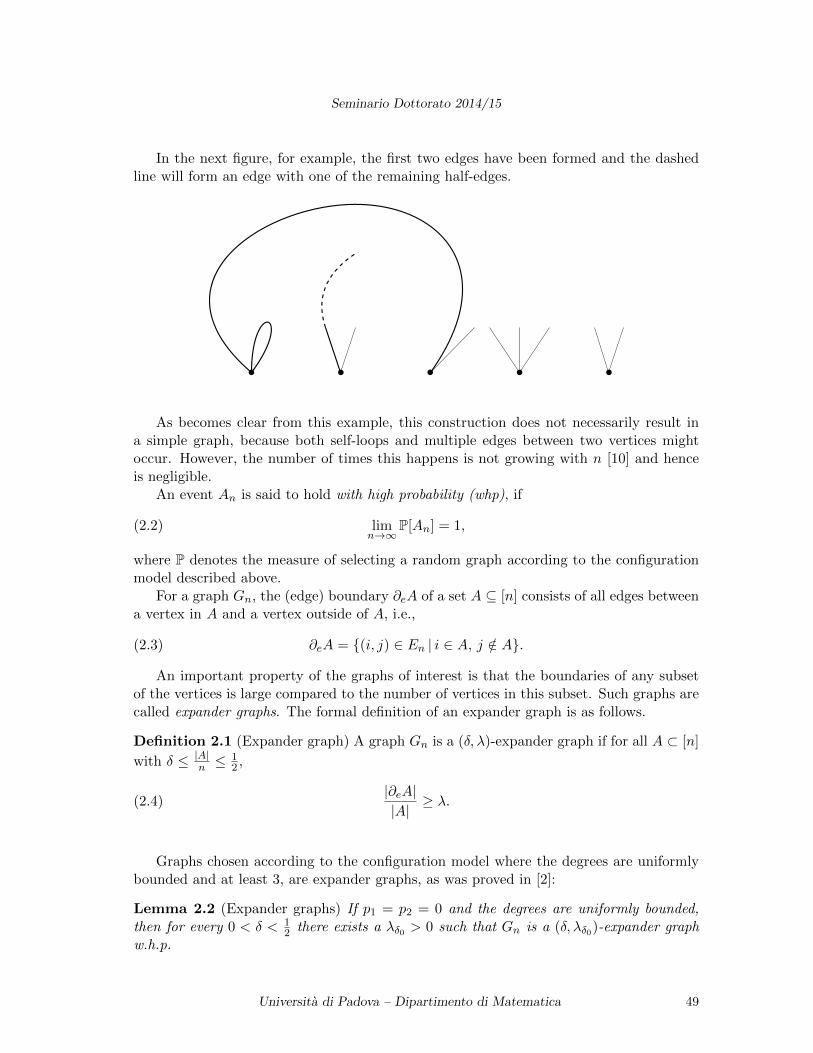
Seminario Dottorato 2014/15
In the next figure, for example, the first two edges have been formed and the dashedline will form an edge with one of the remaining half-edges.
As becomes clear from this example, this construction does not necessarily result ina simple graph, because both self-loops and multiple edges between two vertices mightoccur. However, the number of times this happens is not growing with n [10] and henceis negligible.
An event An is said to hold with high probability (whp), if
(2.2) limn→∞
P[An] = 1,
where P denotes the measure of selecting a random graph according to the configurationmodel described above.
For a graph Gn, the (edge) boundary ∂eA of a set A ⊆ [n] consists of all edges betweena vertex in A and a vertex outside of A, i.e.,
(2.3) ∂eA = (i, j) ∈ En | i ∈ A, j /∈ A.
An important property of the graphs of interest is that the boundaries of any subsetof the vertices is large compared to the number of vertices in this subset. Such graphs arecalled expander graphs. The formal definition of an expander graph is as follows.
Definition 2.1 (Expander graph) A graph Gn is a (δ, λ)-expander graph if for all A ⊂ [n]
with δ ≤ |A|n ≤12 ,
(2.4)|∂eA||A|
≥ λ.
Graphs chosen according to the configuration model where the degrees are uniformlybounded and at least 3, are expander graphs, as was proved in [2]:
Lemma 2.2 (Expander graphs) If p1 = p2 = 0 and the degrees are uniformly bounded,then for every 0 < δ < 1
2 there exists a λδ0 > 0 such that Gn is a (δ, λδ0)-expander graphw.h.p.
Universita di Padova – Dipartimento di Matematica 49
Seminario Dottorato 2014/15
A related quantity is the so-called isoperimetric number, which is defined as follows:
Definition 2.3 (Isoperimetric number) For a graph Gn, the (edge) isoperimetric numberof Gn equals
(2.5) ie(Gn) = minA⊂[n]
|A|≤n/2
|∂eA||A|
,
where |A| denotes the cardinality of the set A.
This definition implies that any graph is a (0, ie(Gn))-expander graph. When all de-grees are equal to r ≥ 3, such graphs are called r-regular graphs, then good bounds onthe isoperimetric number are known as proved in [4, 1].
Lemma 2.4 (Bounds on isoperimetric number) Let Gn be a random r-regular graph withr ≥ 3. Then, whp, there exists a constant C > 0 such that
(2.6)r
2−√
log 2√r ≤ ie(Gn) ≤ r
2− C√r.
The above shows that these random graphs behave in a significantly different way then,for example, the lattice Zd. If you look at a box [`]d ⊂ Zd then the boundary of this boxgrows like `d−1 and the number of vertices in the box like `d. Hence, by letting ` → ∞,we get that the isoperimetric number of Zd equals 0.
3 Ising model
The Ising model on a graph Gn is defined as follows. To each vertex i ∈ [n] we assign aspin σi ∈ −1,+1 and we denote a configuration by σ = (σi)i∈[n]. We define an energyfunction H(σ) : −1,+1n 7→ R, as
(3.1) H(σ) = −J∑
(i,j)∈En
σiσj − h∑i∈[n]
σi,
where J > 0 is the interaction constant and h ∈ R is the external magnetic field. H(σ) iscalled the Hamiltonian.
The probability that in equilibrium the system has configuration σ is then given byBoltzmann-Gibbs measure which is defined as
(3.2) µn(σ) =1
Zne−βH(σ),
where β = 1/T ≥ 0 is the inverse temperature and Zn is the normalization factor, calledthe partition function, i.e.,
(3.3) Zn =∑
σ∈−1,+1ne−βH(σ).
Universita di Padova – Dipartimento di Matematica 50
Seminario Dottorato 2014/15
Without loss of generality, we assume that J = 1, since this is just a rescaling of β and h.From this it becomes clear that spins in the graph that are neighbors of each other
indeed tend to align, because if these spins have the same sign then the energy is lower,and hence the probability that this happens is higher.
For a set A ⊆ [n], denote by σA the configuration where
(3.4) σAi =
+1, if i ∈ A,−1, if i /∈ A.
We also denote = σ∅ and = σ[n], the all minus and all plus configurations, respectively.We often identify the vertex and its spin, e.g., we say that vertex i has a + neighbor ifthere is a vertex j such that (i, j) ∈ En with σj = +1.
Many results about the equilibrium solution for the Ising model on random graphshave been obtained, see, for example, [5, 7, 8].
4 Dynamics of the Ising model and metastability
Besides looking at the Ising model at equilibrium, we can also look at this model whenthe spins evolve in time. We let the system evolve according to Glauber dynamics withMetropolis rates. That is, we consider a discrete time Markov chain where at every timestep we select one of the n spins uniformly at random. If flipping this spin (changing itfrom − to + or from + to −) results in a configuration with lower energy, this spin isalways flipped. If the energy is going up by flipping this spin, the spin is flipped withprobability e−β∆H , where ∆H is the energy difference. If β is large this means that thisis very unlikely to happen (but not impossible).
More formally, we can write the transition probabilities c(σA, σB) from configurationσA to σB as
(4.1) c(σA, σB) =
1ne−β[H(σB)−H(σA)]+ , if |A4B| = 1;
1−∑
B:|A4B|=11ne−β[H(σB)−H(σA)]+ , if A = B,
0, otherwise,
where A4B is the symmetric difference between sets A and B, and [a]+ = maxa, 0. Wedenote by Pη the law of the process starting from configuration η.
The time at which the process visits the configuration σ for the first time if the processstarts from η is called the hitting time of σ and is denoted by τσ. When studying metasta-bility, the problem is to find the hitting time of the stable configuration if the systemstarts in a metastable configuration. We now define what it means for a configuration tobe (meta)stable.
The stable state is the state for which the Hamiltonian is minimal. Throughout therest of this note we assume that h > 0, so that it is obvious from (3.1) that the stablestate is .
To define metastable states, we need to define the communication height between twoconfigurations σ and σ′ which is given by
(4.2) Φ(σ, σ′) = minω path from σ to σ′
maxσ′′∈ω
H(σ′′),
Universita di Padova – Dipartimento di Matematica 51
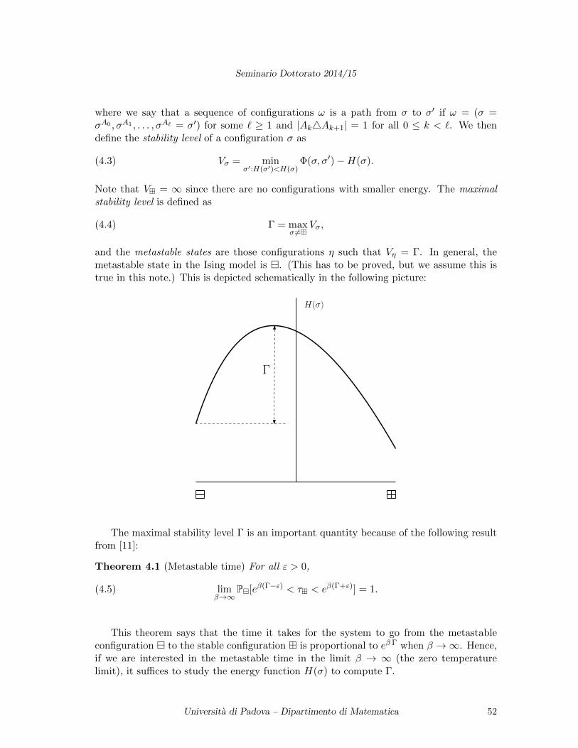
Seminario Dottorato 2014/15
where we say that a sequence of configurations ω is a path from σ to σ′ if ω = (σ =σA0 , σA1 , . . . , σA` = σ′) for some ` ≥ 1 and |Ak4Ak+1| = 1 for all 0 ≤ k < `. We thendefine the stability level of a configuration σ as
(4.3) Vσ = minσ′:H(σ′)<H(σ)
Φ(σ, σ′)−H(σ).
Note that V = ∞ since there are no configurations with smaller energy. The maximalstability level is defined as
(4.4) Γ = maxσ 6=
Vσ,
and the metastable states are those configurations η such that Vη = Γ. In general, themetastable state in the Ising model is . (This has to be proved, but we assume this istrue in this note.) This is depicted schematically in the following picture:
H(σ)
Γ
The maximal stability level Γ is an important quantity because of the following resultfrom [11]:
Theorem 4.1 (Metastable time) For all ε > 0,
(4.5) limβ→∞
P[eβ(Γ−ε) < τ < eβ(Γ+ε)] = 1.
This theorem says that the time it takes for the system to go from the metastableconfiguration to the stable configuration is proportional to eβ Γ when β →∞. Hence,if we are interested in the metastable time in the limit β → ∞ (the zero temperaturelimit), it suffices to study the energy function H(σ) to compute Γ.
Universita di Padova – Dipartimento di Matematica 52
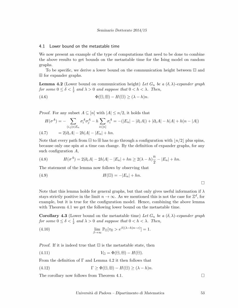
Seminario Dottorato 2014/15
4.1 Lower bound on the metastable time
We now present an example of the type of computations that need to be done to combinethe above results to get bounds on the metastable time for the Ising model on randomgraphs.
To be specific, we derive a lower bound on the communication height between and for expander graphs.
Lemma 4.2 (Lower bound on communication height) Let Gn be a (δ, λ)-expander graphfor some 0 ≤ δ < 1
2 and λ > 0 and suppose that 0 < h < λ. Then,
(4.6) Φ(,)−H() ≥ (λ− h)n.
Proof. For any subset A ⊆ [n] with |A| ≤ n/2, it holds that
H(σA) = −∑
(i,j)∈En
σAi σAj − h
∑i∈[n]
σAi = −(|En| − |∂eA|) + |∂eA| − h|A|+ h(n− |A|)
= 2|∂eA| − 2h|A| − |En|+ hn.(4.7)
Note that every path from to has to go through a configuration with bn/2c plus spins,because only one spin at a time can change. By the definition of expander graphs, for anysuch configuration A,
(4.8) H(σA) = 2|∂eA| − 2h|A| − |En|+ hn ≥ 2(λ− h)n
2− |En|+ hn.
The statement of the lemma now follows by observing that
(4.9) H() = −|En|+ hn.
Note that this lemma holds for general graphs, but that only gives useful information if λstays strictly positive in the limit n→∞. As we mentioned this is not the case for Zd, forexample, but it is true for the configuration model. Hence, combining the above lemmawith Theorem 4.1 we get the following lower bound on the metastable time.
Corollary 4.3 (Lower bound on the metastable time) Let Gn be a (δ, λ)-expander graphfor some 0 ≤ δ < 1
2 and λ > 0 and suppose that 0 < h < λ. Then,
(4.10) limβ→∞
P[τ > eβ((λ−h)n−ε)] = 1.
Proof. If it is indeed true that is the metastable state, then
(4.11) V = Φ(,)−H().
From the definition of Γ and Lemma 4.2 it then follows that
(4.12) Γ ≥ Φ(,)−H() ≥ (λ− h)n.
The corollary now follows from Theorem 4.1.
Universita di Padova – Dipartimento di Matematica 53
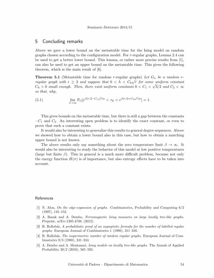
Seminario Dottorato 2014/15
5 Concluding remarks
Above we gave a lower bound on the metastable time for the Ising model on randomgraphs chosen according to the configuration model. For r-regular graphs, Lemma 2.4 canbe used to get a better lower bound. This lemma, or rather more precise results from [1],can also be used to get an upper bound on the metastable time. This gives the followingtheorem, which is the main result of [6].
Theorem 5.1 (Metastable time for random r-regular graphs) Let Gn be a random r-regular graph with r ≥ 3 and suppose that 0 < h < C0
√r for some uniform constant
C0 > 0 small enough. Then, there exist uniform constants 0 < C1 <√
3/2 and C2 < ∞so that, whp,
(5.1) limβ→∞
P[eβ(r/2−C1√r)n < τ < eβ(r/2+C2
√r)n] = 1.
This gives bounds on the metastable time, but there is still a gap between the constants−C1 and C2. An interesting open problem is to identify the exact constant, or even toprove that such a constant exists.
It would also be interesting to generalize this results to general degree sequences. Abovewe showed how to obtain a lower bound also in this case, but how to obtain a matchingupper bound is not known.
The above results only say something about the zero temperature limit β → ∞. Itwould also be interesting to study the behavior of this model at low positive temperatures(large but finite β). This in general is a much more difficult problem, because not onlythe energy function H(σ) is of importance, but also entropy effects have to be taken intoaccount.
References
[1] N. Alon, On the edge-expansion of graphs. Combinatorics, Probability and Computing 6/2(1997), 145–152.
[2] A. Basak and A. Dembo, Ferromagnetic Ising measures on large locally tree-like graphs.Preprint, arXiv:1205.4749, (2012).
[3] B. Bollobas, A probabilistic proof of an asymptotic formula for the number of labelled regulargraphs. European Journal of Combinatorics 1 (1980), 311–316.
[4] B. Bollobas, The isoperimetric number of random regular graphs. European Journal of Com-binatorics 9/3 (1988), 241–244.
[5] A. Dembo and A. Montanari, Ising models on locally tree-like graphs. The Annals of AppliedProbability 20/2 (2010), 565–592.
Universita di Padova – Dipartimento di Matematica 54
Seminario Dottorato 2014/15
[6] S. Dommers, Metastability of the Ising model on random regular graphs at zero temperature.Preprint, arXiv:1411.6802 (2014).
[7] S. Dommers, C. Giardina and R. van der Hofstad, Ising models on power-law random graphs.Journal of Statistical Physics 141/4 (2010),638–660.
[8] S. Dommers, C. Giardina and R. van der Hofstad, Ising critical exponents on random treesand graphs. Communications in Mathematical Physics 328/1 (2014), 355–395.
[9] P. Erdos and A. Renyi, On the evolution of random graphs. Publications of the MathematicalInstitute of the Hungarian Academy of Science 5 (1960), 17–61.
[10] R. van der Hofstad, “Random graphs and complex networks”. Lecture notes available at theurl http://www.win.tue.nl/~rhofstad/NotesRGCN.html (2014).
[11] F. Manzo, F.R. Nardi, E. Olivieri and E. Scoppola, On the essential features of metastability:tunnelling time and critical configurations. Journal of Statistical Physics 115/1-2 (2004), 591–642.
[12] M. E. J. Newman, The structure and function of complex networks. SIAM Review 45/2(2003),167–256.
[13] M. Niss, History of the Lenz–Ising model 1920–1950: from ferromagnetic to cooperative phe-nomena. Archive for History of Exact Sciences 59/3 (2005), 267–318.
[14] M. Niss, History of the Lenz–Ising model 1950–1965: from irrelevance to relevance. Archivefor History of Exact Sciences 63/3 (2009), 243–287.
[15] M. Niss, History of the Lenz–Ising model 1965–1971: the role of a simple model in under-standing critical phenomena. Archive for History of Exact Sciences 65/6 (2011), 625–658.
Universita di Padova – Dipartimento di Matematica 55
Seminario Dottorato 2014/15
Automorphism-invariant modules
Nguyen Khanh Tung (∗)
Abstract. In this note we mention the class of injective modules, the class of quasi-injective modulesand their generalization, the class of automorphism-invariant modules. Then we give some resultsrelated to the endomorphism rings of automophism-invariant modules and their injective envelopesand show a connection between automorphism-invariant modules and bolean rings.
1 Introduction
The important of injective modules in Module Theory and more generally in Algebra be-came obvious in the 1960s and 1970s largely through the lecture note of Carl Faith [10].Since that time there has been a continuing interest in such modules and their variousgeneralization which arose directly from the study of injective modules. Many resultsobatined for injective modules could be transfered readily to quasi-injective modules. Oneof generalizations of the class of quasi-injective modules is the class of automorphism-invariant modules. A module M is called automorphism-invariant if it is invariant underautomorphisms of its injective envelope, that is, if ϕ(M) ⊆ M for every ϕ ∈ Aut(E(M))(equivalently, if ϕ(M) = M for every ϕ ∈ Aut(E(M))). It is showed that every di-rect summand of automorphism-invariant modules is automorphism-invariant and theclass of automorphism-invariant modules satisfies Condition (C2) and (C3). However, anautomorphism-invariant module satisfy Condition (C1) if and only if it is quasi-injective.Moreover, we will see that if M is an automorphism-invariant module, then
End(M)/J(End(M))
turns out to be a rationally closed subring of
End(E(M))/J(End(E(M))).
Both the rings End(M)/J(End(M)) and End(E(M))/J(End(E(M))) are von Neumannregular [12, Proposition 1]. We consider in particular the case of automorphism-invariantmodules of finite Goldie dimension or indecomposable. Notice that automorphism-invariantmodules have the exchange property [12], so that indecomposable automorphism-invariant
(∗)Ph.D. course, Universita di Padova, Dip. Matematica, via Trieste 63, I-35121 Padova, Italy; E-mail:. Seminar held on February 25th, 2015.
Universita di Padova – Dipartimento di Matematica 56
Seminario Dottorato 2014/15
modules have a local endomorphism ring. Furthermore, idempotents can be lifted moduloevery right ideal both in End(M) and in End(E(M)) [17]. We then study the connec-tion between automorphism-invariant modules and boolean rings. The existence of such aconnection is from the results in Section 5 of [20], where Vamos considers modules whoseendomorphism ring (or endomorphism ring modulo the Jacobson radical) is a boolean ring.He studies modules in which the identity endomorphism is the sum of two automorphisms.This condition is related to the existence of factors of the endomorphism ring isomorphic tothe field F2 with two elements [13]. Notice that if M is an automorphism-invariant rightR-module and End(M) has no factor isomorphic to F2, then M is quasi-injective [11,Theorem 3]. Every automorphism-invariant module is the direct sum of a quasi-injectivemodule and a square-free module [7, Theorem 3]. This leads us to study, for automorphism-invariant square-free modules M , the relation between M being quasi-injective and theexistence of factors isomorphic to F2 in End(M) and in End(E(M)).
Throughout, all rings have identity element and modules are right unital. For a moduleM , E(M) denotes the injective envelope of M .
2 Injective and Quasi-Injective Modules
In this section, we introduduce injective and quasi-injective modules as well as their basicproperties that will be necessary to study automorphism-invariant modules. All resultsare well-known and can be found in most text-book of ring theory or module theory. Werefer the reader to [1] and [14].
Definition 2.1 Let ER,MR be two modules. We say that ER is injective relative toMR (or ER is M -injective) if, for each monomorphism f : KR →MR and each morphismg : KR → ER, there exists a morphism h : MR → ER with h f = g.
Definition 2.2 A module E is injective if E is injective relative to every module, thatis, for every monomorphism f : K → M and every morphism g : K → E, there existsa morphism h : M → E such that g = h f. A ring R is right selft-injective if RR isinjective.
In the next Proposition, we give a further criterion to determine injective modules,that is, a further characterization of injective modules.
Proposition 2.3 (Baer’s criterion) The following about a module E are equivalent:
(a) E is injective.
(b) E is injective relative to R.
(c) For every right ideal I ≤ RR and every morphism h : I → E there exists an x ∈ Esuch that h(a) = xa (a ∈ I).
Example 2.4 An abelian group G is divisible if nG = G for every non zero integer n.Hence G is divisible if and only if, for every g ∈ G and every n > 0, there exists h ∈ G
Universita di Padova – Dipartimento di Matematica 57
Seminario Dottorato 2014/15
such that g = nh. A Z-module G is injective if and only if it is a divisible abelian group.For instance, the abelian group Z is not divisible, and the abelian group Q is divisible.Hence, Q is injective.
Definition 2.5 An injective envelope of a module MR is a pair (ER, i) where ER is aninjective right R-module and i : MR → ER is an essential monomorphism.
Theorem 2.6 Every right R-module has a unique injective envelope up to isomorphism.
Definition 2.7 A module MR is called quasi-injective if M is M -injective.
Theorem 2.8 (R. E. Johnson and E. T. Wong, 1961) Let M be a module. Then M isquasi-injective if and only if it is invariant under every endomorphism of E(M).
Example 2.9 Let R = Z/4Z and M = 2Z/4Z. Then M is quasi-injective but notinjective.
3 Automorphism-Invariant Modules
The aim of this section is to give a presentation of some known and new results onautomorphism-invariant modules and related notions.
Definition 3.1 A module M is called automorphism-invariant if it is invariant underautomorphisms of its injective envelope, that is, if ϕ(M) ⊆ M for every ϕ ∈ Aut(E(M))(equivalently, if ϕ(M) = M for every ϕ ∈ Aut(E(M))).
It is showed that a module M is quasi-injective if and only if it is invariant un-der endomorphisms of its injective envelopes (Theorem 2.8). So every quasi-injectiveis automorphism-invariant. But the converse is not true by the following example.
Example 3.2 Let R consists of all (xn)n∈N ∈∏n∈N Z2 such that all except finitely many
xn are equal to some a ∈ Z2. Then R is a ring, and E(RR) =∏n∈N Z2. Because End(SR)
has only one automorphism, namely the identity, R is automorphism-invariant but it isnot quasi-injective.
Definition 3.3 A module M satisfies Condition (C1) if every submodule of M is essentialin a direct summand of M .
Definition 3.4 A module M satisfies Condition (C2) if every submodule of M isomorphicto a direct summand of M is also a direct summand of M .
Definition 3.5 A module M satisfies Condition (C3) if, for any two direct summandsN1, N2 of M with N1 ∩N2 = 0, the direct sum N1 ⊕N2 is a direct summand of M .
Universita di Padova – Dipartimento di Matematica 58
Seminario Dottorato 2014/15
It is well known that every injective (quasi-injective) module satisfies Condition (Ci) (i =1, 2, 3) (see [14] or [16]). The following results show that automorphism-invariant modulesalways satisfy Condition (C2) and (C3), but do not satisfy Condition (C1) in general.
Proposition 3.6 (T.-K. Lee and Y. Zhou, 2013) An automorphism-invariant modulesatisfies Condition (C1) if and only if it is quasi-injective.
Proposition 3.7 (T.-K. Lee and Y. Zhou, 2013) Every automorphism-invariant modulesatisfies Condition (C3).
Definition 3.8 A module M is called pseudo-injective if, for any submodule A of M,every monomorphism f : A→M can be extended to an element of End(M).
Theorem 3.9 (N. Er, S. Singh and A. K. Srivastava, 2013) Automorphism-invariant mod-ules are precisely pseudo-injective modules.
Proposition 3.10 (H. Q. Dinh, 2005) Every pseudo-injective satisfies Condition (C2).
Corollary 3.11 Every automorphism-invariant satisfies Condition (C2).
As the cases of injective and quasi-injective modules, a direct summand of an auto-morphism-invariant module inherits the property by the next proposition.
Proposition 3.12 (T.-K. Lee and Y. Zhou, 2013) Every direct summand of an automor-phism-invariant is automorphism-invariant.
Before stating some results about the endomorphism rings of automorphism-invariantmodules, we review some necessary concepts.
Definition 3.13 A ring morphism ϕ : R → S is local if, for every r ∈ R, ϕ(r) invertiblein S implies r invertible in R.
Proposition 3.14 A ring morphism ϕ : R→ S is local if and only if Kerϕ ≤ J(R) andϕ(U(R)) = ϕ(R)∩U(S) where U(R) and U(S) is the group of invertible elements of ringsR,S respectively.
Definition 3.15 A rationally closed subring of a ring S is a subring R of S such thatthe embedding R → S is a local morphism, that is, a subring R of S such that U(R) =R ∩ U(S).
Let M be a right R-module. From now we denote E(M) the injective envelope of M.Let ∆ be denote the set of all endomorphisms with essential kernel. The next propositioncharacterizes the Jacobson radical of the endomorphism rings of automorphism-invariantmodules.
Universita di Padova – Dipartimento di Matematica 59
Seminario Dottorato 2014/15
Proposition 3.16 (P. A. Guil Asensio and A. K. Srivastava, 2013) Let M be an automorphism-invariant module. Then the Jacobson radical of End(M) is ∆, End(M)/J(End(M)) is avon Neumann regular ring and idempotents can be lifted modulo J(End(M)).
More properties about the endomorphism of automorphism-invariant modules are pro-vided by the following results.
Theorem 3.17 (A. Alahmadi and A. Facchini and N. K. Tung, 2015) Let M be anautomorphism-invariant module and E(M) be its injective envelope. Then
(a) There is a canonical local morphism
ϕ : End(M)→ End(E(M))/J(End(E(M)))
with kernel J(End(M)), so that ϕ induces an embedding ϕ, as a rationally closed sub-ring, of the von Neumann regular ring End(M)/J(End(M)) into the von Neumannregular right self-injective ring
End(E(M))/J(End(E(M))).
(b) For every invertible element v of the ring End(E(M))/J(End(E(M))), there existsan invertible element u of End(M)/J(End(M)) such that ϕ(u) = v.
(c) For every idempotent element f of the ring End(E(M))/J(End(E(M))) there existsan idempotent element e of End(M)/J(End(M)) such that ϕ(e) = f if and only ifthe module M is quasi-injective.
(d) If M is quasi-injective, then ϕ is an isomorphism.
Proposition 3.18 (A. Alahmadi and A. Facchini and N. K. Tung, 2015) Let M be anautomorphism-invariant module. Then
(a) If M is indecomposable, then End(M) is a local ring.
(b) If M has finite Goldie dimension, then every injective endomorphism of M is anautomorphism of M and the endomorphism ring End(M) is a semiperfect ring.
Corollary 3.19 (A. Alahmadi and A. Facchini and N. K. Tung, 2015) If M,N are twoautomorphism-invariant R-modules of finite Goldie dimensions isomorphic to submodulesof each other, then M is isomorphic to N .
Proposition 3.20 (A. Alahmadi and A. Facchini and N. K. Tung, 2015) The followingconditions are equivalent for a ring R.
(a) Every automorphism-invariant R-module of finite Goldie dimension is quasi-injective.
Universita di Padova – Dipartimento di Matematica 60
Seminario Dottorato 2014/15
(b) Every automorphism-invariant indecomposable R-module of finite Goldie dimensionis uniform.
(c) Every automorphism-invariant indecomposable R-module of finite Goldie dimensionis quasi-injective.
A non-zero ring R is a boolean ring if every element of R is idempotent. A ring isboolean if and only if it is isomorphic to a subring of FX2 , where X is a non-empty set. Thenext theorem gives us a sufficient condition so that an automorphism-invariant module isquasi-injective.
Theorem 3.21 (P. A. Guil Asensio and A. K. Srivastava, 2014) Let M be a right modulesuch that End(M) has no factor isomorphic to F2. Then M is quasi-injective if and onlyif M is automorphism-invariant.
Recall that two modules are said to be orthogonal if they do not contain nonzeroisomorphic submodules.
Proposition 3.22 (A. Alahmadi and A. Facchini and N. K. Tung, 2015) Let M = M1⊕M2
be an automorphism-invariant R-module where M1 and M2 are orthogonal. Then End(M)has no factor isomorphic to F2 if and only if each End(Mi) (i = 1, 2) has no factorisormophic to F2.
Definition 3.23 A module M is square-free if it does not contain a direct sum of twonon-zero isomorphic submodules.
Theorem 3.24 (N. Er, S. Singh and A. K. Srivastava, 2013) Every automorphism-invariantmodule M decomposes as a direct sum M = X ⊕ Y , where X is quasi-injective, Y is asquare-free module orthogonal to X, and X and Y are relatively injective modules.
The previous theorem reduces studying automorphism-invariant modules to consider-ing automophism-invariant square-free modules.
Lemma 3.24.1 (A. Alahmadi and A. Facchini and N. K. Tung, 2015) If M1,M2 are tworight modules over a ring R and M1,M2 have isomorphic injective envelopes, which arenon-zero modules, then M1 and M2 have non-zero isomorphic submodules.
Corollary 3.25 (A. Alahmadi and A. Facchini and N. K. Tung, 2015) If M is an auto-morphism-invariant square-free module, then every injective endomorphism of M is anautomorphism of M .
Corollary 3.26 (A. Alahmadi and A. Facchini and N. K. Tung, 2015) If M,N are twoautomorphism-invariant square-free R-modules isomorphic to submodules of each other,then M is isomorphic to N .
Universita di Padova – Dipartimento di Matematica 61
Seminario Dottorato 2014/15
Proposition 3.27 (A. Alahmadi and A. Facchini and N. K. Tung, 2015) Let M be anautomorphism-invariant module and E(M) be its injective envelope. The following condi-tions are equivalent:
(a) M is square-free.
(b) E(M) is square-free.
(c) The von Neumann regular ring End(M)/J(End(M)) is abelian.
(d) The von Neumann regular right self-injective ring End(E(M))/J(End(E(M))) isabelian.
Theorem 3.28 (A. Alahmadi and A. Facchini and N. K. Tung, 2015) Let M be anautomorphism-invariant module and let E(M) be its injective envelope.
(a) If M is quasi-injective and End(M) has a factor isomorphic to F2, then End(E(M))has a factor isomorphic to F2.
(b) If M has finite Goldie dimension and End(M) has a factor isomorphic to F2, thenthe following conditions hold.
(i) End(E(M)) has a factor isomorphic to F2.
(ii) E(M) has a direct-sum decomposition E(M) = E⊕C with E orthogonal to C,E an indecomposable R-module and End(E)/J(End(E)) ∼= F2.
(iii) Aut(E) = 1 + J(End(E)), so that every automorphism of the R-module E isthe identity on an essential R-submodule of E.
(iv) E is the injective envelope of its non-zero R-submodule annE(2).
References
[1] D. W. Anderson and K. R. Fuller, “Rings and Categories of Modules”. Second Edition, GTM13, Springer-Verlag, New York, 1992.
[2] A. Alahmadi, A. Facchini and Nguyen Khanh Tung, Automorphism-invariant modules. Toappear in Rend. Sem. Mat. Univ. Padova (2015).
[3] B. Brainerd and J. Lambek, On the ring of quotients of a boolean ring. Canad. Math. Bull. 2(1959), 25–29.
[4] T. T. Bumby, Modules which are isomorphic to submodules of each other. Arch. Math. 16(1965), 184–185.
Universita di Padova – Dipartimento di Matematica 62
Seminario Dottorato 2014/15
[5] R. Camps and W. Dicks, On semilocal rings. Israel J. Math. 81 (1993), 203–211.
[6] H. Q. Dinh, A note on pseudo-injective modules. Comm. Algebra 33 (2005), 361–369.
[7] N. Er, S. Singh and A. K. Srivastava, Rings and modules which are stable under automorphismsof their injective hulls. J. Algebra 379 (2013), 223–229.
[8] A. Facchini, “Module Theory. Endomorphism rings and direct sum decompositions in someclasses of modules”. Progress in Math. 167, Birkhauser Verlag, Basel, 1998. Reprinted inModern Birkhauser Classics, Birkhauser Verlag, Basel, 2010.
[9] A. Facchini and D. Herbera, Local morphisms and modules with a semilocal endomorphismring. Algebr. Represent. Theory 9 (2006), 403–422.
[10] C. Faith, “Lectures on injective modules and quotient rings”. Springer LNM 49 (1967).
[11] P. A. Guil Asensio and A. K. Srivastava, Additive unit representations in endomorphism ringsand an extension of a result of Dickson and Fuller. In: “Ring Theory and its Applications”,Contemp. Math. 609, Amer. Math. Soc., Providence 2014, D. V. Huynh, et al., eds., pp.117–121.
[12] P. A. Guil Asensio and A. K. Srivastava, Automorphism-invariant modules satisfy the exchangeproperty. J. Algebra 388 (2013), 101–106.
[13] D. Khurana and A. K. Srivastava, Right self-injective rings in which every element is a sumof two units. J. Algebra Appl. 6 (2007), 281–286.
[14] T. Y. Lam, “Lectures on Modules and Rings”. Springer-Verlag, New York, 1998.
[15] T.-K. Lee and Y. Zhou, Modules which are invariant under automorphisms of their injectivehulls. J. Algebra Appl. 12 (2013).
[16] S. H. Mohamed and B. J. Muller, “Continuous and Discrete Modules”. London MathematicalSociety, Lecture Notes Series 147, Cambridge University Press, 1990.
[17] W. K. Nicholson, Lifting idempotents and exchange rings. Trans. Amer. Math. Soc. 229 (1977),269–278.
[18] S. Singh and A. K. Srivastava, Rings of invariant module type and automorphism-invariantmodules. Contemp. Math. AMS, in press; available in http://arxiv.org/pdf/1207.5370.pdf.
[19] B. Stenstrom, “Rings of quotients”. Springer-Verlag, Berlin-Heidelberg-New York, 1975.
[20] P. Vamos, 2-good rings. Quart. J. Math. 56 (2005), 417–430.
Universita di Padova – Dipartimento di Matematica 63
Seminario Dottorato 2014/15
Introduction to kernel-based methods
Gabriele Santin (∗)
This note is a brief introduction to the theory of kernel based methods, with particularfocus on approximation in kernel based spaces.
Kernel-based methods are emerging in various fields of applied mathematics as a tech-nique to solve several kind of problems. Kernel-based algorithm are successfully applied inapproximation theory, in machine learning, in geostatistics and in different type of numer-ical simulations in engineering. The use of such methods is motivated by reasons that varyfrom field to field, but it is mainly due to their flexibility and to the simple structure thatis shared by all the particular algorithms. In particular, in the field of approximation the-ory, kernel-based methods can be proven to be error optimal both in solving interpolationproblems and recovery of solution of certain PDEs.
In the following we will give an introduction to the use of kernels. The focus will be onapproximation, but the underlying theory is the same used in all the applications. Furtherdetails on the topics presented in this note can be found in the monographs [1, 2, 3].
1 Statement of the problem and motivation
We are interested in the following recovery problem in Rd. We are given a set of n ∈ Npairwise distinct points Xn = x1, . . . , xn ⊂ Ω ⊂ Rd, where Ω is a bounded set, and avector of values Fn = [f1, . . . , fn]T ∈ Rn. The vector Fn is understood as a collection ofsampling of an unknown continuous function f : Ω→ R, but for now we consider only then values fi.
Given this set of data, we consider a linear scheme to find a continuous functionsn : Ω→ R that interpolates the data, i.e., s(xi) = fi, 1 ≤ i ≤ n. To do so, one considersa suitable n-dimensional trial space V = spanvi, . . . , vn, where vj : Ω → R are linearlyindependent continuous functions, and an interpolant
sn =
n∑j=1
cjvj ,
for an unknown coefficient vector c = [c1, . . . , cn]T ⊂ Rn such that sn(xi) = fi, 1 ≤ i ≤ n.
(∗)Ph.D. course, Universita di Padova, Dip. Matematica, via Trieste 63, I-35121 Padova, Italy; E-mail:. Seminar held on March 18th, 2015.
Universita di Padova – Dipartimento di Matematica 64
Seminario Dottorato 2014/15
A minimal requirement for a scheme to be well posed is the existence of a uniquefunction sn ∈ V that interpolates the data, for any given set of data. This is equivalentto require that V is an Haar space.
Definition 1 An n-dimensional linear space V ⊂ C(Ω) is an Haar space of dimension non Ω if for any set Xn of pairwise distinct point in Ω and any set of values Fn ∈ Rn thereexist a unique function sn ∈ V such that sn(xi) = fi, 1 ≤ i ≤ n.
A typical example of an Haar space of dimension n in R is the space of univariate realpolynomials of degree n − 1, that is to say, the (n − 1)-degree polynomial interpolant ona set of n distinct points is always uniquely defined.
The situation is completely different if d > 1.
Theorem 1 (Mairhuber - Curtis) If Ω ⊂ Rd, d > 1, contains an interior point, thereexists no Haar spaces on Ω of dimension n > 1.
The theorem tells us that for d > 1, except for the trivial case n = 1, one can notchoose a fixed trial space V , but it is necessary to adapt it to each particular set of data.A strategy to overcome this problem comes from the use of kernels and we will see that,in some circumstances, it is also the unique optimal strategy.
2 From kernel interpolation to Hilbert spaces
A kernel K on a set S is a positive definite and symmetric function K : S×S → R, wherepositive definiteness is defined in the following sense.
Definition 2 A function K : S × S → R is positive definite if, for any n ∈ N, forany set x1, . . . , xn ⊂ S of pairwise distinct elements and for any vector of coefficientsc = [c1, . . . , cn]T ∈ Rn,
n∑i=1
n∑j=1
cicjK(xi, xj) ≥ 0.
If the above expression is zero only for c = 0, the function is strictly positive definite.
Although the theory can be developed for positive definite kernels, we will restrict thefollowing discussion to strictly positive definite kernels, to which we will refer simply askernels. Most of the results are true in both cases, but dealing with vanishing bilinear formsrequires more technical details. Moreover, in this note we will only consider continuouskernels defined on bounded subspaces Ω of Rd, even if kernels can be constructed onabstract sets S with almost no structure (e.g., kernels defined on sets of strings or ontrees and graphs are commonly used in Machine Learning; also, complex valued kernelsare studied in differential geometry and analysis).
To have a concrete example in mind, we recall that the Gaussian kernel K(x, y) =e−ε
2‖x−y‖, ε > 0, is in fact a kernel on Rd, for all d.
Universita di Padova – Dipartimento di Matematica 65
Seminario Dottorato 2014/15
2.1 Kernel-based interpolation
Given a kernel, the interpolation problem can be simply solved in the following way. Wecan build point-dependent trial spaces through translates of the kernel, i.e.,
V (Xn) = spanK(·, xi) : 1 ≤ i ≤ n,
hence look for interpolants in the form
sn =n∑j=1
cjK(·, xj),
for some unknown vector of coefficients c ∈ Rn. The vector c is determined by theinterpolation conditions sn(xi) = fi, 1 ≤ i ≤ n, i.e., by the solution of the linear system
Ac = Fn,
where the kernel matrix A = [K(xi, xj)]ni,j=1 ∈ Rn×n is symmetric and positive definite
by the definition of kernel, and it is in particular invertible for any set of pairwise distinctpoints. In other words, the interpolation problem is well posed for any data.
We just mention here that the actual computation of the solution of the above linearsystem is in general an hard task since the kernel matrix is usually ill-conditioned, and itshould not be solved directly. Nevertheless, several methods are available to compute c ina stable way, and the topic is currently an active field of research.
2.2 Kernel-based spaces
What we described so far is just a procedure to construct a continuous function withprescribed values at prescribed points. Now we would like to see if this is an effectiveapproximation method. Namely, we assume that the data values are samples of a functionf : Ω→ R, i.e., fi = f(xi), 1 ≤ i ≤ n, and we will investigate the relation between f andsn. In particular, we will characterize the space of functions that can be recovered witharbitrary accuracy by the above procedure, provided n is sufficiently large.
First, observe that for any x ∈ Ω the functions K(·, x) : Ω→ R and all the finite linearcombination of functions of this kind can be exactly recovered, simply by choosing as Xn
all the points used to construct the kernel translates. We denote as H0(Ω) the set of allthese functions, i.e.,
H0(Ω) = spanK(·, x) : x ∈ Ω.
On H0(Ω) is possible to define the bilinear form n∑j=1
cjK(·, xj),m∑i=1
diK(·, yi)
K
:=n∑j=1
m∑i=1
cjdiK(xj , yi).
and since K is a kernel, and it is in particular symmetric and strictly positive definite,this bilinear form defines an inner product on H0(Ω).
Universita di Padova – Dipartimento di Matematica 66
Seminario Dottorato 2014/15
The closure of H0(Ω) with respect to the norm induced by (·, ·)K is an Hilbert spaceHK(Ω) of functions on Ω to R, and it is called the native space of the kernel K on Ω. Wewill still denote by (·, ·)K its inner product.
The native space of K is in fact the natural space where kernel approximation takesplace, and in enjoys some useful property that are listed in the following theorem.
Theorem 2 The space HK(Ω) is a reproducing kernel Hilbert space (RKHS) with kernelK, i.e.,
(a) K(·, y) ∈ HK(Ω) for all y ∈ Ω,
(b) (f,K(·, x))K = f(x) for all f ∈ HK(Ω), x ∈ Ω,
and it is the unique RKHS with kernel K on Ω. Moreover,
(c) If f ∈ HK(Ω) then ‖f − sn‖K → 0 as n→∞,
(d) if there exists a positive constant Cf such that ‖sn‖K ≤ Cf for any finite set Xn ⊂ Ω,for any n ∈ N, then f ∈ HK(Ω) and ‖f‖K is the minimal possible value for theconstant Cf .
We now know how to solve the interpolation problem, how to build an Hilbert spaceof functions starting from a kernel, and that this space contains precisely (in the sense ofproperties (c), (d)) all the functions that can be approximated by the kernel method.
A question that naturally arises is if this is the only way to solve the interpolationproblem. We will see in the next Section that one can in fact go the other way round, i.e.,start with a quite general Hilbert space and prove that kernel interpolation is the optimalrecovery strategy in that space.
Before moving to the next Section, observe that working in a RKHS is very useful toconstruct numerical approximation schemes. First, to compute norms of functions in thedense subspace H0(Ω) it is enough to evaluate the kernel at some points. Second, thanksto property (b) of Theorem 2, norm convergence in HK(Ω) implies pointwise convergence.Indeed, if f, g ∈ HK(Ω),
|(f − g)(x)| = |(f − g,K(·, x)K | ≤ ‖f − g‖K‖K(·, x)‖K≤ ‖f − g‖K
√K(x, x) for all x ∈ Ω.
3 From Hilbert spaces to kernel interpolation
We now assume to have an Hilbert space H of functions from Ω to R, and we want tointerpolate a given function in H at prescribed, but arbitrary, points Xn ⊂ Ω. Given thistask, since we want to recover a function from its pointwise samples, it make sense toassume that the pointwise evaluation functionals δx are continuous in H. We are then inthe following situation.
Theorem 3 A Hilbert space H of functions from Ω to R is a reproducing kernel Hilbertspace if and only if the pointwise evaluation functionals δx are continuous for any x ∈ Ω.
Universita di Padova – Dipartimento di Matematica 67
Seminario Dottorato 2014/15
In this case, the kernel of the space is the Riesz representer of these functional, that is tosay,
δx(f) = (f,K(·, x))H for all f ∈ H, x ∈ Ω.
Moreover, the kernel is strictly positive definite if and only if all the functionals δx : x ∈Ω are linearly independent.
As the Theorem proves, kernel-based spaces are quite common. Examples of suchspaces are the following:
• any Hilbert space of finite dimension N is a RKHS. If vjNj=1 is any orthonormal
basis of this space, the kernel is K(x, y) =∑N
j=1 vj(x)vj(y), x, y ∈ Ω;
• the Sobolev space H10 ((0, 1)) is a RKHS. Its kernel is the Brownian bridge kernel
K(x, y) = min(x, y)− xy, x, y ∈ (0, 1);
• the Sobolev spaces Hβ(Rd), β > d/2 are RKHS, whose kernels are the β-Maternkernels, which can be expressed in terms of Bessel’s functions.
Under the assumption of continuity of the functionals δx, we are left to work in thenative space of a given kernel K. We will hence still use the notation HK(Ω) for this spaceand (·, ·)K for its inner product.
3.1 Optimal recovery
Going back to the interpolation problem, it is clear that the method described in theprevious sections is well defined here. In particular, the trial space V (Xn) is a finitedimensional subspace of HK(Ω), and we can define an interpolation operator
Sn : HK(Ω)→ V (Xn)
f 7→ sn.
where the interpolating function sn is defined as above. The next Theorem shows thatthis is in fact the unique optimal interpolation strategy in HK(Ω).
Theorem 4 The kernel interpolant sn is the minimal norm interpolant in HK(Ω), i.e.,
sn = min‖tn‖K : tn ∈ HK(Ω), tn(xi) = f(xi), 1 ≤ i ≤ n.
Moreover, the interpolation operator Sn coincides with the HK(Ω)-projection into the sub-space V (Xn), thus, in particular, the interpolant is also the ‖ · ‖K-best approximant off .
3.2 The power function and a simple error estimate
To conclude this note, we recall the basic error estimate on kernel approximation.
Universita di Padova – Dipartimento di Matematica 68
Seminario Dottorato 2014/15
Namely, although we introduced this method in order to being able to deal with scat-tered data, there is obviously a dependence of the approximation error upon the distribu-tion of the points in Xn. To measure this distribution it is customary to introduce the filldistance hXn,Ω,
hXn,Ω = supx∈Ω
minxi∈Xn
‖x− xi‖,
which corresponds to the radius of the biggest ball that can be put in Ω without pointsof Xn.
The error estimate is computed by bounding the power function Pn, that is the norm ofthe pointwise approximation error. Namely, since the interpolation operator is a boundedoperator in HK(Ω), we can compute the norm of the functional Ex := δx (id− Sn),
Ex : HK(Ω)→ HK(Ω)
f 7→ f(x)− sn(x).
The norm of this functional is the power function, and it can be computed as
P2n(x) = K(x, x)−
n∑j=1
vj(x)2, x ∈ Ω,
where vjnj=1 is any orthonormal basis of V (Xn). Of course, for any f ∈ HK(Ω), it holds
|f(x)− sn(x)| ≤ Pn(x)‖f‖K , x ∈ Ω.
The next Theorem uses this relation and a bound on the power function to have a boundon the pointwise approximation error.
Theorem 5 If Ω is bounded and satisfies an interior cone condition, and K ∈ C2k(Ω×Ω),there exists positive constants h0 and C such that, for all Xn with hXn,Ω ≤ h0,
|f(x)− sn(x)| ≤ ChkXn,Ω‖f‖K , x ∈ Ω.
References
[1] M. Buhmann, “Radial Basis Functions, Theory and Implementations”. Cambridge UniversityPress, 2003.
[2] G. F. Fasshauer, “Meshfree Approximation Methods with MATLAB”. World Scientific Pub-lishers, Singapore, 2007.
[3] H. Wendland, “Scattered Data Approximation”. Cambridge University Press, Cambridge,2005.
Universita di Padova – Dipartimento di Matematica 69
Seminario Dottorato 2014/15
A short introduction to Berkovich
affine line over the field Cp
Velibor Bojkovic (∗)
Abstract. In this note we present a construction of the Berkovich affine line over the field Cp,which is a p-adic analogue of the complex plane C. We emphasize on how one can visualize itstree-structure as well as explain what are its building blocks: both as a set and as a topologicalspace. We end by describing a connection between general Berkovich compact, connected, smoothcurves over Cp and (the reduction of) their semistable models over Fp.
1 Introduction: from Q to Cp
1.1 p-adic norm on Q
Let us start by recalling the definition of a norm on Q.
Definition 1.1 A norm on Q is a mapping | · | : Q → R≥0, x 7→ |x| which satisfies thefollowing three conditions:
(a) |x| = 0 iff x = 0,
(b) |xy| = |x||y|,
(c) |x+ y| ≤ |x|+ |y| for all x, y ∈ Q .
Example 1.2
(a) We all know the standard absolute value | · |∞ on Q (| − 2|∞ = 2, |95 |∞ = 95 ).
(b) Let c ∈ (0, 1), then |x|∞,c := |x|c∞ is also a norm on Q.
(c) The trivial absolute value | · |0 (|0| = 0 |x| = 1, x 6= 0).
(∗)Ph.D. course, Universita di Padova, Dip. Matematica, via Trieste 63, I-35121 Padova, Italy; E-mail:. Seminar held on April 1st, 2015.
Universita di Padova – Dipartimento di Matematica 70
Seminario Dottorato 2014/15
Exercise 1.3 Prove that | · |∞,c is really a norm on Q.
The main example of a norm on Q in this note is the so-called p-adic norm, where pis a prime number.
Definition 1.4 Let p ∈ Π, where Π is the set of prime numbers, and let x ∈ Q. Letus write x = a
b = pα a′
b′ where (p, a′) = (p, b′) = 1, and α ∈ Z. We define a function| · |p : Q→ R≥0 as x 7→ |x|p = p−α.
Theorem 1.5 The map | · |p is a norm on Q.
Exercise 1.6 Prove the following:
(a) | · |p is a norm on Q;
(b) For c ∈ (0, 1), | · |p,c := | · |cp is also a norm;
(c) p-adic norm is ultrametric, i.e. it satisfies the strong triangle inequality |x + y|p ≤max(|x|p, |y|p).
One may notice that the norms | · |p and | · |)p,c are more ”similar” than, for example,the norms | · |p and | · |∞, the similarity at this point being understood intuitively. Forexample, the sequence (pn)n converges in each of the norms | · |p,c but it doesn’t convergein none of the norms | · |∞,c, To make things formal, we recall the following.
Definition 1.7 We say that two norms | · |1 and | · |2 are equivalent if |x|1 < 1 iff |x|2 < 1.
The following celebrated theorem due to Ostrowski classifies all the norms on Q up toequivalence.
Theorem 1.8 (Ostrowski’s Theorem) Every norm on Q is either | · |0, or it is equivalentto | · |∞ or to | · |p for some p ∈ Π.
1.2 The field Cp
From the first course on mathematical analysis one knows that the fields R and C areobtained from Q by first completing with respect to the standard absolute value | · |∞ (thisgives R) and then taking the algebraic closure of R (to obtain C). Then, one proves aswell that C is complete.
What happens if we do the same procedure for Q (i.e. completing and then takingthe algebraic closure) with respect to the p-adic norm | · |p?
Definition 1.9 We define Qp to be completion of Qp with respect to the p-adic norm| · |p, and call it the p-adic field.
One may think about field Qp as of an analogue of the field R. However, when onetakes the algebraic closure of Qp, the obtained field Qp doesn’t really represent an analogue
Universita di Padova – Dipartimento di Matematica 71

Seminario Dottorato 2014/15
of the field C, as the following exercise suggests. Notice that | · |p canonically extends toQp, and we call the extension as well the p-adic norm and use | · |p to denote it.
Exercise 1.10 Prove that the algebraic closure Qp of Qp is not complete.
Definition 1.11 The p-adic completion of the field Qp is denoted by Cp.
It turns out that the field Cp is algebraically closed and complete, and as such one maythink of it as the p-adic analogue of the field of complex numbers C. But, it seems thatall the analogy stops here, as the following short list of properties suggests, and which isleft as an exercise.
Exercise 1.12
(a) Prove that the field Cp equiped with the topology induced by the norm | · |p is totallydisconnected. (Recall that the topological space is said to be totally disconnected ifthe maximal connected subsets are just points.)
(b) Let B(a, r), where a ∈ Cp and r ∈ R>0 be the closed disc in Cp with center in a andof radius r, i.e. the set of points b ∈ Cp, |a − b|p ≤ r. Prove that every point inB(a, r) is a center of it.
(c) Let a, b, c ∈ Cp. Prove that the ”triangle” with vertices in a, b, c is isoscele.
(d) Prove that the rim z ∈ Cp, |z| = 1 is both open and closed in p-adic topology.
(e) Let B(0, r) ⊂ Cp as above. Can you give an example of a continuous, locally constantfunction f : B(0, 1) → R which is not constant? Can this happen if we take thedisc B(0, r) ⊂ C? Why not?
And now, to the motivational question of this note: How one can do analytic geometryover a field such as Cp? What would for example be an equivalent over Cp of the classicalcomplex plane/affine line over C?
In the next sections we present a short introduction to the Berkovich theory of analyticspaces over normed fields, which answers in a satisfactory way the previous questions.
2 Berkovich affine line A1Cp
2.1 Berkovich spectrum of a normed ring
Definition 2.1 A normed commutative ring A is a commutative ring A equipped with afunction | · | : A→ R≥0 which satisfies the following conditions:
(a) |1| = 1 and |f | = 0 iff f = 0,
(b) |f · g| ≤ |f | · |g|,
Universita di Padova – Dipartimento di Matematica 72
Seminario Dottorato 2014/15
(c) |f + g| ≤ |f |+ |g|,
Definition 2.2 Let A be a commutative ring (assumed to be with unit). A multiplicativeseminorm on A is a function | · | : A→ R≥0 such that
(a) |0| = 0 and |1| = 1,
(b) |f · g| = |f ||g|,
(c) |f + g| ≤ |f |+ |g|.
Definition 2.3 Let A be a normed ring, with norm || · ||. The Berkovich spectrum of thering A is the setM(A) of all the multiplicative seminorms | · | on A which are bounded bythe norm || · ||. We say that | · | is bounded by || · || if there exists a positive real constantC such that for all f ∈ A, |f | < C||f ||. We equip the setM(A) with the weakest topologysuch that the functions, f :M(A)→ R≥0, where f ∈ A and given by |·| ∈ M 7→ |f | ∈ R≥0
are continuous.
We have the following fundamental theorem by Berkovich (see [1]).
Theorem 2.4 Let A be a commutative ring. Then,
(a) If A is nonzero, M(A) is nonempty.
(b) If A is complete, M(A) is compact.
Exercise 2.5 Let A be the ring Z equipped with the standard norm | · |∞. Then Z is acomplete ring. Find M(Z). What is M(Z) if we equip Z with the trivial norm?
Remark 2.6 The general idea for doing analytic geometry over the field Cp, whichwould be analogous to the complex analytic geometry over C, is to start with Cp-rings offunctions (in the theory so-called Cp-affinoid algebras) that would correspond to classicalcomplex holomorphic functions, and then to assign Berkovich spectrum to such rings (ofcourse, Cp-affinoid algebras come already with a norm, so there is no problem here).
2.2 The set A1Cp
Definition 2.7 The Berkovich affine line over Cp, A1Cp , is defined to be the set of multi-
plicative seminorms on the polynomial ring Cp[T ] extending the p-adic norm of Cp. Thetopology of A1
Cp is the weakest one such that all the functions f(T ) ∈ Cp[T ] which act on
A1Cp by | · | 7→ |f(T )| ∈ R≥0 are continuous.
Remark 2.8 Note a slight difference with respect to taking the Berkovich spectrum ofthe polynomial ring. First of all, we didn’t assume any norm on Cp[T ] so we couldn’t just
Universita di Padova – Dipartimento di Matematica 73
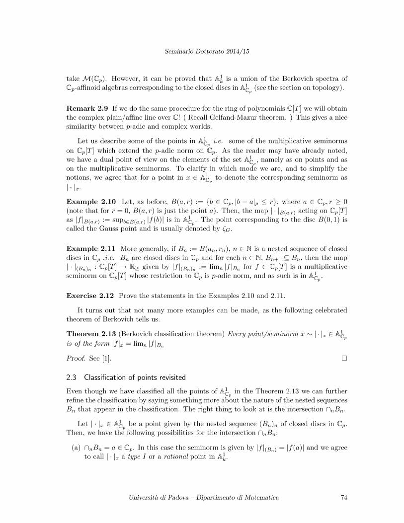
Seminario Dottorato 2014/15
take M(Cp). However, it can be proved that A1k is a union of the Berkovich spectra of
Cp-affinoid algebras corresponding to the closed discs in A1Cp (see the section on topology).
Remark 2.9 If we do the same procedure for the ring of polynomials C[T ] we will obtainthe complex plain/affine line over C! ( Recall Gelfand-Mazur theorem. ) This gives a nicesimilarity between p-adic and complex worlds.
Let us describe some of the points in A1Cp i.e. some of the multiplicative seminorms
on Cp[T ] which extend the p-adic norm on Cp. As the reader may have already noted,we have a dual point of view on the elements of the set A1
Cp , namely as on points and ason the multiplicative seminorms. To clarify in which mode we are, and to simplify thenotions, we agree that for a point in x ∈ A1
Cp to denote the corresponding seminorm as
| · |x.
Example 2.10 Let, as before, B(a, r) := b ∈ Cp, |b − a|p ≤ r, where a ∈ Cp, r ≥ 0(note that for r = 0, B(a, r) is just the point a). Then, the map | · |B(a,r) acting on Cp[T ]as |f |B(a,r) := supb∈B(a,r) |f(b)| is in A1
Cp . The point corresponding to the disc B(0, 1) iscalled the Gauss point and is usually denoted by ζG.
Example 2.11 More generally, if Bn := B(an, rn), n ∈ N is a nested sequence of closeddiscs in Cp ,i.e. Bn are closed discs in Cp and for each n ∈ N, Bn+1 ⊆ Bn, then the map| · |(Bn)n : Cp[T ] → R≥ given by |f |(Bn)n := limn |f |Bn for f ∈ Cp[T ] is a multiplicativeseminorm on Cp[T ] whose restriction to Cp is p-adic norm, and as such is in A1
Cp .
Exercise 2.12 Prove the statements in the Examples 2.10 and 2.11.
It turns out that not many more examples can be made, as the following celebratedtheorem of Berkovich tells us.
Theorem 2.13 (Berkovich classification theorem) Every point/seminorm x ∼ | · |x ∈ A1Cp
is of the form |f |x = limn |f |Bn
Proof. See [1].
2.3 Classification of points revisited
Even though we have classified all the points of A1Cp in the Theorem 2.13 we can further
refine the classification by saying something more about the nature of the nested sequencesBn that appear in the classification. The right thing to look at is the intersection ∩nBn.
Let | · |x ∈ A1Cp be a point given by the nested sequence (Bn)n of closed discs in Cp.
Then, we have the following possibilities for the intersection ∩nBn:
(a) ∩nBn = a ∈ Cp. In this case the seminorm is given by |f |(Bn) = |f(a)| and we agreeto call | · |x a type I or a rational point in A1
k.
Universita di Padova – Dipartimento di Matematica 74
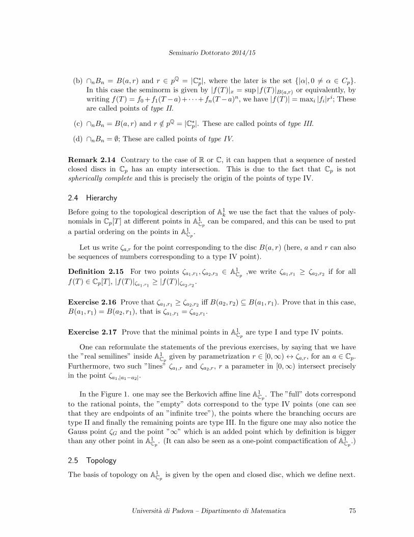
Seminario Dottorato 2014/15
(b) ∩nBn = B(a, r) and r ∈ pQ = |C∗p|, where the later is the set |α|, 0 6= α ∈ Cp.In this case the seminorm is given by |f(T )|x = sup |f(T )|B(a,r) or equivalently, bywriting f(T ) = f0 +f1(T −a)+ · · ·+fn(T −a)n, we have |f(T )| = maxi |fi|ri; Theseare called points of type II.
(c) ∩nBn = B(a, r) and r /∈ pQ = |C∗p|. These are called points of type III.
(d) ∩nBn = ∅; These are called points of type IV.
Remark 2.14 Contrary to the case of R or C, it can happen that a sequence of nestedclosed discs in Cp has an empty intersection. This is due to the fact that Cp is notspherically complete and this is precisely the origin of the points of type IV.
2.4 Hierarchy
Before going to the topological description of A1k we use the fact that the values of poly-
nomials in Cp[T ] at different points in A1Cp can be compared, and this can be used to put
a partial ordering on the points in A1Cp .
Let us write ζa,r for the point corresponding to the disc B(a, r) (here, a and r can alsobe sequences of numbers corresponding to a type IV point).
Definition 2.15 For two points ζa1,r1 , ζa2,r3 ∈ A1Cp ,we write ζa1,r1 ≥ ζa2,r2 if for all
f(T ) ∈ Cp[T ], |f(T )|ζa1,r1 ≥ |f(T )|ζa2,r2 .
Exercise 2.16 Prove that ζa1,r1 ≥ ζa2,r2 iff B(a2, r2) ⊆ B(a1, r1). Prove that in this case,B(a1, r1) = B(a2, r1), that is ζa1,r1 = ζa2,r1 .
Exercise 2.17 Prove that the minimal points in A1Cp are type I and type IV points.
One can reformulate the statements of the previous exercises, by saying that we havethe ”real semilines” inside A1
Cp given by parametrization r ∈ [0,∞)↔ ζa,r, for an a ∈ Cp.Furthermore, two such ”lines” ζa1,r and ζa2,r, r a parameter in [0,∞) intersect preciselyin the point ζa1,|a1−a2|.
In the Figure 1. one may see the Berkovich affine line A1Cp . The ”full” dots correspond
to the rational points, the ”empty” dots correspond to the type IV points (one can seethat they are endpoints of an ”infinite tree”), the points where the branching occurs aretype II and finally the remaining points are type III. In the figure one may also notice theGauss point ζG and the point ”∞” which is an added point which by definition is biggerthan any other point in A1
Cp . (It can also be seen as a one-point compactification of A1Cp .)
2.5 Topology
The basis of topology on A1Cp is given by the open and closed disc, which we define next.
Universita di Padova – Dipartimento di Matematica 75
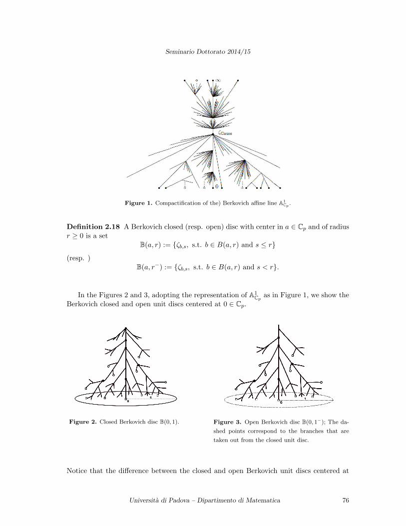
Seminario Dottorato 2014/15
Figure 1. Compactification of the) Berkovich affine line A1Cp
.
Definition 2.18 A Berkovich closed (resp. open) disc with center in a ∈ Cp and of radiusr ≥ 0 is a set
B(a, r) := ζb,s, s.t. b ∈ B(a, r) and s ≤ r
(resp. )B(a, r−) := ζb,s, s.t. b ∈ B(a, r) and s < r.
In the Figures 2 and 3, adopting the representation of A1Cp as in Figure 1, we show the
Berkovich closed and open unit discs centered at 0 ∈ Cp.
Figure 2. Closed Berkovich disc B(0, 1). Figure 3. Open Berkovich disc B(0, 1−); The da-
shed points correspond to the branches that are
taken out from the closed unit disc.
Notice that the difference between the closed and open Berkovich unit discs centered at
Universita di Padova – Dipartimento di Matematica 76
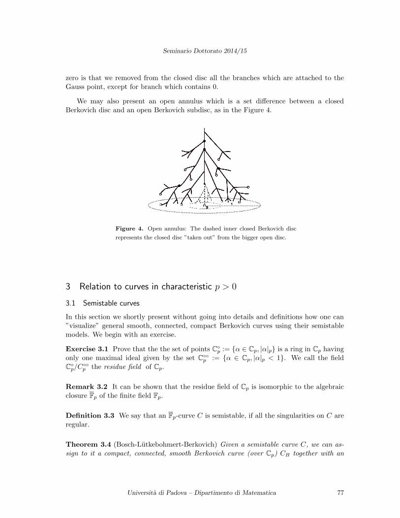
Seminario Dottorato 2014/15
zero is that we removed from the closed disc all the branches which are attached to theGauss point, except for branch which contains 0.
We may also present an open annulus which is a set difference between a closedBerkovich disc and an open Berkovich subdisc, as in the Figure 4.
Figure 4. Open annulus: The dashed inner closed Berkovich disc
represents the closed disc ”taken out” from the bigger open disc.
3 Relation to curves in characteristic p > 0
3.1 Semistable curves
In this section we shortly present without going into details and definitions how one can”visualize” general smooth, connected, compact Berkovich curves using their semistablemodels. We begin with an exercise.
Exercise 3.1 Prove that the the set of points Cp := α ∈ Cp, |α|p is a ring in Cp havingonly one maximal ideal given by the set Cp := α ∈ Cp, |α|p < 1. We call the fieldCp/Cp the residue field of Cp.
Remark 3.2 It can be shown that the residue field of Cp is isomorphic to the algebraicclosure Fp of the finite field Fp.
Definition 3.3 We say that an Fp-curve C is semistable, if all the singularities on C areregular.
Theorem 3.4 (Bosch-Lutkebohmert-Berkovich) Given a semistable curve C, we can as-sign to it a compact, connected, smooth Berkovich curve (over Cp) CB together with an
Universita di Padova – Dipartimento di Matematica 77
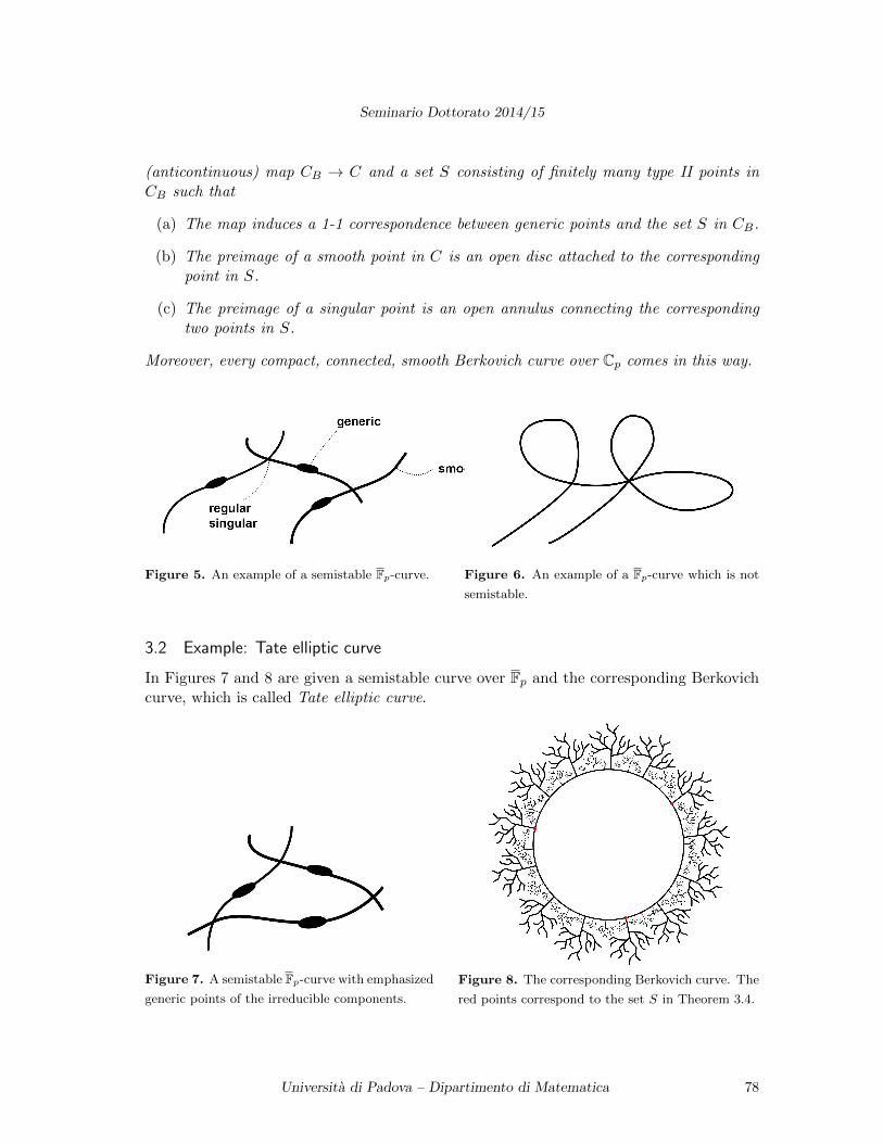
Seminario Dottorato 2014/15
(anticontinuous) map CB → C and a set S consisting of finitely many type II points inCB such that
(a) The map induces a 1-1 correspondence between generic points and the set S in CB.
(b) The preimage of a smooth point in C is an open disc attached to the correspondingpoint in S.
(c) The preimage of a singular point is an open annulus connecting the correspondingtwo points in S.
Moreover, every compact, connected, smooth Berkovich curve over Cp comes in this way.
Figure 5. An example of a semistable Fp-curve. Figure 6. An example of a Fp-curve which is not
semistable.
3.2 Example: Tate elliptic curve
In Figures 7 and 8 are given a semistable curve over Fp and the corresponding Berkovichcurve, which is called Tate elliptic curve.
Figure 7. A semistable Fp-curve with emphasized
generic points of the irreducible components.
Figure 8. The corresponding Berkovich curve. The
red points correspond to the set S in Theorem 3.4.
Universita di Padova – Dipartimento di Matematica 78
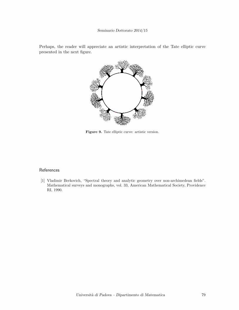
Seminario Dottorato 2014/15
Perhaps, the reader will appreciate an artistic interpretation of the Tate elliptic curvepresented in the next figure.
Figure 9. Tate elliptic curve: artistic version.
References
[1] Vladimir Berkovich, “Spectral theory and analytic geometry over non-archimedean fields”.Mathematical surveys and monographs, vol. 33, American Mathematical Society, ProvidenceRI, 1990.
Universita di Padova – Dipartimento di Matematica 79
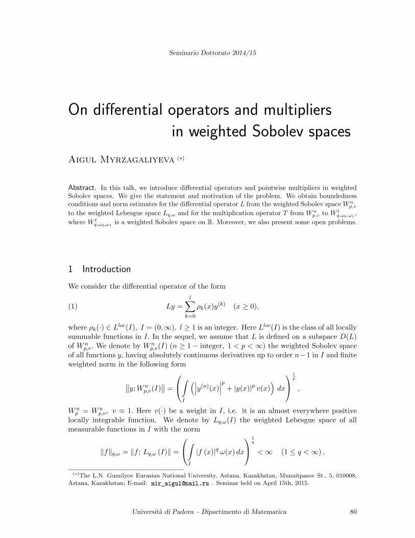
Seminario Dottorato 2014/15
On differential operators and multipliers
in weighted Sobolev spaces
Aigul Myrzagaliyeva (∗)
Abstract. In this talk, we introduce differential operators and pointwise multipliers in weightedSobolev spaces. We give the statement and motivation of the problem. We obtain boundednessconditions and norm estimates for the differential operator L from the weighted Sobolev space Wn
p,v
to the weighted Lebesgue space Lq,ω and for the multiplication operator T from Wnp,v to W l
q,ω0,ω1,
where W lq,ω0,ω1
is a weighted Sobolev space on R. Moreover, we also present some open problems.
1 Introduction
We consider the differential operator of the form
(1) Ly =
l∑k=0
ρk(x)y(k) (x ≥ 0),
where ρk(·) ∈ Lloc(I), I = (0,∞), l ≥ 1 is an integer. Here Lloc(I) is the class of all locallysummable functions in I. In the sequel, we assume that L is defined on a subspace D(L)of Wn
p,v. We denote by Wnp,v(I) (n ≥ 1− integer, 1 < p <∞) the weighted Sobolev space
of all functions y, having absolutely continuous derivatives up to order n−1 in I and finiteweighted norm in the following form
∥∥y;Wnp,v(I)
∥∥ =
∫I
(∣∣∣y(n)(x)∣∣∣p + |y(x)|p v(x)
)dx
1p
,
Wnp = Wn
p,v, v ≡ 1. Here v(·) be a weight in I, i.e. it is an almost everywhere positivelocally integrable function. We denote by Lq,ω(I) the weighted Lebesgue space of allmeasurable functions in I with the norm
‖f‖q,ω = ‖f ; Lq,ω (I)‖ =
∫I
|f (x)|q ω(x) dx
1q
<∞ (1 ≤ q <∞) ,
(∗)The L.N. Gumilyov Eurasian National University, Astana, Kazakhstan, Munaitpasov St., 5, 010008,Astana, Kazakhstan; E-mail: . Seminar held on April 15th, 2015.
Universita di Padova – Dipartimento di Matematica 80
Seminario Dottorato 2014/15
Lq(I) = Lq,ω(I), ω ≡ 1.The purpose of this paper is to obtain conditions for the boundedness of the differential
operator L as an operator acting from Wnp,v(I) to the space Lq,ω(I) and to apply these
results to the study of multipliers in Sobolev spaces.We define as length function in I any positive and right-continuous function h(·)
(h(·) is a l.f.). We denote by ∆(x) the segment [x,x+h(x)] for the l.f. h(·).This paper is organized as follows: In Sec. 2, we introduce Sobolev spaces used as
function spaces and we give some examples to understand why such spaces are important.In Sec. 3, you find basic definitions and notation. In Sec. 4, we present some new resultsformulated as theorems.
2 Sobolev spaces
In mathematics, a Sobolev space is a vector space of functions equipped with a norm thatis a combination of Lp-norms of the function itself as well as its derivatives up to a givenorder. The derivatives are understood in a suitable weak sense to make the space complete,thus a Banach space. Intuitively, the Sobolev space is a space of functions with sufficientlymany derivatives for some application domain, such as partial differential equations. Theirimportance comes from the fact that solutions of partial differential equations are naturallyfound in Sobolev spaces, rather than in spaces of continuous functions. In the twentiethcentury, however, it was observed that the space C1 (or C2, etc.) was not exactly theright space to study solutions of differential equations. Sobolev spaces are the modernreplacement for these spaces in which to look for solutions of partial differential equations.
Let us consider the simplest example the Dirichlet problem for the Laplace equationin a bounded domain Ω ⊂ Rn :
∆u = 0, x ∈ Ω,
u(x) = ϕ(x), x ∈ ∂Ω,
where ϕ(x) is a given function on the boundary ∂Ω. It is known that the Laplace equationis the Euler equation for the functional
l(u) =
∫Ω
n∑j=1
∣∣∣∣ ∂u∂xj∣∣∣∣2 dx.
We can consider this problem as a variational problem: to find the minimum of l(u) on theset of functions satisfying condition u|∂Ω = ϕ. It is much easier to minimize this functionalnot in C1(Ω), but in a larger class. Namely, in the Sobolev class W 1
2 (Ω). W 12 (Ω) consists
of all functions u ∈ L2(Ω), having the weak derivatives ∂u ∈ L2(Ω), j = 1, . . . , n. If theboundary ∂Ω is smooth, then the trace of u(x) on ∂Ω is well defined and relation u|∂Ω = ϕmakes sense. If we consider l(u) on W 1
2 (Ω), it is easy to prove the existence and uniquenessof solution of our variational problem. The function u ∈ W 1
2 (Ω), that gives minimum tol(u) under the condition u|∂Ω = ϕ, is called the weak solution of the Dirichlet problem forthe Laplacian.
Universita di Padova – Dipartimento di Matematica 81
Seminario Dottorato 2014/15
Let us consider the following exterior Oseen problem to clarify the importance of theweighted Sobolev space:
−∆u+ k ∂u∂x1
+∇π = 0 in Ω−,
divu = 0 in Ω−,
u = u∗ on ∂Ω−,
where Ω− ≡ R3\Ω, Ω = B(0, 1). The data are the boundary value u∗ and a real k > 0. Theproblem consists of looking for the velocity field u of the fluid and the pressure functionπ.
We introduce the weight function ρ(x) = 1+ |x|. Let us assume that (u, π) is a solutionof the problem and (u, π) equal to the fundamental solution of the Oseen system, which isof class C∞ in Ω−. Then the boundary data u∗ is just the restriction to ∂Ω− = ∂Ω. As wecan easily show, the component u of the fundamental solution behaves like 1
ρ at infinity
and accordingly is not in W 12 (Ω−). However, it is in the weighted Sobolev space W 1
2,ρ(Ω−).
3 Preliminaries and notation
Definition 1 (See [1]) A weighted function v in I is called admissible with respect to thelength function h(·), if there exist 0 < δ < 1, 0 < τ ≤ 1, such that the following inequalityis true
(2) h(x)n− 1
p infe
∫∆(x)\e
v(t) dt
1p
≥ τ
for all x ∈ I.
In (2) the infimum is taken over all measurable subset e of ∆(x) with Lebesgue measure|e| ≤ δ |∆(x)| . We denote by Πn,p(δ, τ) the set of admissible weights v with respect to thel.f. h(·).
We give some examples.
Example 1 Since
h(x)n− 1
p infe
∫∆(x)\e
v(t) dt
1p
= infe
∫[x,x+1]\e
dt
1p
≥ (1− δ)1p = τ,
the function v = 1 is admissible with respect to the l.f. h(·) = 1.
Definition 2 We say that a function ω(·) satisfies the slow variation condition withrespect to the l.f. h(·), if there exist constants 0 < b1 < 1 < b2 such that
(3) b1ω(x) ≤ ω(t) ≤ b2ω(x) for all t ∈ ∆(x).
Universita di Padova – Dipartimento di Matematica 82
Seminario Dottorato 2014/15
Example 2 Let v satisfy the slow variation condition (3) with respect to the l.f. h(x) = v(x)− 1np .
Then v is admissible with respect to the l.f. h(x) = v(x)− 1np when τp = b1(1 − δ). The
proof is trivial.
Every power function v (x) = (1 + |x|)µ , 0 < µ < +∞ satisfies the slow variation
condition with respect to the l.f. h (x) = (1 + x)− µnp . Indeed,(
1 + t
1 + x
)µ≤(
1 + x+ h(x)
1 + x
)µ=
(1 +
(1
1 + x
)1+ µnp
)µ≤ 2µ = b2,(
1 + t
1 + x
)µ=
(1 + x+ t− x
1 + x
)µ=
(1 +
t− x1 + x
)µ≥ 1 > 2−µ = b1
for all t ∈ ∆(x).
Definition 3 We say that a weight v satisfies the condition A(δ,β) (0 < δ, β < 1) withrespect to the length function h(·) in I if for any interval ∆ = [a, b] ⊂ ∆(x) = [x, x+h(x)](x ≥ 0) and any measurable subset e of ∆ with the Lebesgue measure |e| ≤ δ|∆| thefollowing inequality holds ∫
e
v(t) dt ≤ β∫∆
v(t) dt.
We denote by A(δ,β) the set of all weights v which satisfy the condition A(δ,β). For example,
if b2b−11 δ < 1 in (3), then v ∈ A(δ,β) with β = b2b
−11 δ.
Let v∗ be a Otelbayev function. Namely
v∗(x) = suph>0
h : hpn−1
x+h∫x
v(t) dt ≤ 1
(see [2]). We first show that 0 < v∗(x) <∞ for all x ≥ 0. To do this, we note that
M(x, h; v)def= hpn−1
x+h∫x
v(t) dt −−−−→h→0+
0
and that M(x, h; v)→∞ if h→∞. Hence, there exist δx > 0 and Tx > 0, such that
M(x, h; v) ≤ 1, if 0 < h ≤ δx,M(x, h; v) > 1, if h ≥ Tx.
Therefore, we obtain
(0, δx) ⊂ Hx,v = h > 0: M(x, h; v) ≤ 1 ⊂ (0, Tx),
δx ≤ supHx,v = v∗(x) ≤ Tx.
Universita di Padova – Dipartimento di Matematica 83
Seminario Dottorato 2014/15
The function v∗ is continuous in I. By using absolute continuity property of the integralwe can imply that
v∗(x)pn−1
x+v∗(x)∫x
v(t) dt = 1.
Example 3 Any weight v ∈ A(δ,β) with respect to the l.f. h(x) = v∗(x) in I is admissiblewith respect to the l.f. h(x) = v∗(x). Thus, for all e ⊂ ∆∗(x) = [x, x+ v∗(x)] with themeasure |e| ≤ δ|∆∗(x)|, we have
v∗(x)pn−1
∫∆∗(x)\e
v(t) dt = v∗(x)pn−1
∫∆∗(x)
v(t) dt−∫e
v(t) dt
≥≥ (1− β)v∗(x)pn−1
∫∆∗(x)
v(t) dt = 1− β = τ.
Let Cn[a, b] (−∞ < a < b <∞) be the space of all functions y, having continuousderivative up to order n in [a, b].
Proposition 1 (see [3]) Let 1 ≤ p < ∞. Then there exist constants A(n, j), A(n, j, p),j = 0, 1, 2, . . . , n− 1 such that(4)
maxa≤x≤b
∣∣∣y(j)(x)∣∣∣ ≤ A(n, j)(b− a)n−j−1/p
b∫a
∣∣∣y(n)(t)∣∣∣p dt+ (b− a)−np
b∫a
|y(t)|p dt
1/p
,
(5)∥∥∥y(j);Lp[ a, b]
∥∥∥ ≤ A(n, j, p)(b− a)n−j∥∥∥y(n);Lp[ a, b]
∥∥∥+ (b− a)−n ‖y;Lp[ a, b]‖
for all functions y(·) ∈ Cn[a, b]. Here we understand that the symbols A(n, j), A(n, j, p)denote the best choice of the constants in (4), (5).
Lemma 1 Let v belong to Πn,p(δ, τ) with respect to the l.f. h(·). Then there exists aconstant C∗ = C∗(δ, τ) > 1 independent of v(·) such that the following estimate is true
(6) h(x)−npx+h(x)∫x
|y|p dt ≤ C∗x+h(x)∫x
(∣∣∣y(n)∣∣∣p + |y|p v(t)
)dt (x ≥ 0)
for all y ∈ Cn (∆) , where ∆ = [x, x+ h(x)].
Universita di Padova – Dipartimento di Matematica 84
Seminario Dottorato 2014/15
4 Main results
4.1 One dimensional differential operators in weighted Sobolev spaces W np,v
Theorem 1 Let n > 1 be an integer. Let 1 < p ≤ q <∞. Let v belong to Πn,p(δ, τ) withrespect to the l.f. h(·). Let
Rk = supx≥0
h(x)n−k− 1
p
x+h(x)∫x
|ρk(t)|q dω(t)
1q
<∞
for k = 0, 1, . . . , l (dω(t) = ω(t)dt) . Then the operator L in (1) is bounded from Wnp,v(I)
to Lq,ω(I). Here the norm has the following form
(7)∥∥L; Wn
p,v(I)→ Lq,ω(I)∥∥ ≤ C l∑
k=0
Rk,
where C = (1 + C∗)1p
l∑k=0
A(n, k).
Let us assume that the operator L in (1) is bounded as an operator from Wnp,v to Lq,ω,
i.e. D(L) ⊂ Wnp,v and there exists a constant K > 0 such that
(8)
∫I
|Ly|q dω(t)
1q
≤ K‖y; Wnp,v‖ (y ∈ D(L)).
Theorem 2 Let 1 < p, q < ∞. Let the operator L in (1) be bounded from Wnp,v to Lq,ω.
Then
(9) Rk = supx≥0
v∗(x)n−k− 1
p
x+
3v∗(x)4∫
x+v∗(x)
4
|ρk(t)|q dω(t)
1q
≤ Ck∥∥L; Wn
p,v → Lq,ω∥∥ ,
where the constant Ck > 0 does not depend on ρk (0 ≤ k ≤ l), ω, v.
We set
R∗ =l∑
k=0
supx≥0
v∗(x)n−k− 1
p
x+v∗(x)∫x
|ρk(t)|q dω
1q
,
R∗ =
l∑k=0
supx≥1
v∗(x)n−k− 1
p
x+
3v∗(x)4∫
x+v∗(x)
4
|ρk(t)|q dω
1q
.
Universita di Padova – Dipartimento di Matematica 85
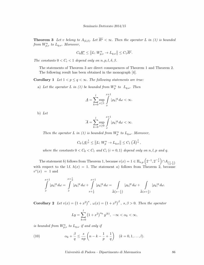
Seminario Dottorato 2014/15
Theorem 3 Let v belong to A(δ,β). Let R∗ < ∞. Then the operator L in (1) is boundedfrom Wn
p,v to Lq,ω. Moreover,
C0R∗ ≤
∥∥L; Wnp,v → Lq,ω
∥∥ ≤ C1R∗.
The constants 0 < Ci < 1 depend only on n, p, l, δ, β.
The statements of Theorem 3 are direct consequences of Theorem 1 and Theorem 2.The following result has been obtained in the monograph [4].
Corollary 1 Let 1 < p ≤ q <∞. The following statements are true:
a) Let the operator L in (1) be bounded from Wnp to Lq,ω. Then
A =
l∑k=0
supx≥1
x+1∫x
|ρk|q dω <∞.
b) Let
A =l∑
k=0
supx≥0
x+1∫x
|ρk|q dω <∞.
Then the operator L in (1) is bounded from Wnp to Lq,ω. Moreover,
C0 (A)1q ≤
∥∥L; Wnp → Lq,ω
∥∥ ≤ C1
(A) 1q ,
where the constants 0 < C0 < C1 and Ci (i = 0, 1) depend only on n, l, p and q.
The statement b) follows from Theorem 1, because v(x) = 1 ∈ Πn,p
(2−1, 2
− 1p
)∩A( 1
2, 12)
with respect to the l.f. h(x) = 1. The statement a) follows from Theorem 2, becausev∗(x) = 1 and
x+1∫x
|ρk|q dω =
x+ 12∫
x
|ρk|q dω +
x+1∫x+ 1
2
|ρk|q dω =
∫∆(x− 1
4)
|ρk|q dω +
∫∆(x+ 1
4)
|ρk|q dω.
Corollary 2 Let v(x) =(1 + x2
)s, ω(x) =
(1 + x2
)β, s, β > 0. Then the operator
Ly =
l∑k=0
(1 + x2
)αk y(k), −∞ < αk <∞,
is bounded from Wnp,v to Lq,ω if and only if
(10) αk +β
q≤ s
np
(n− k − 1
p+
1
q
)(k = 0, 1, . . . , l).
Universita di Padova – Dipartimento di Matematica 86
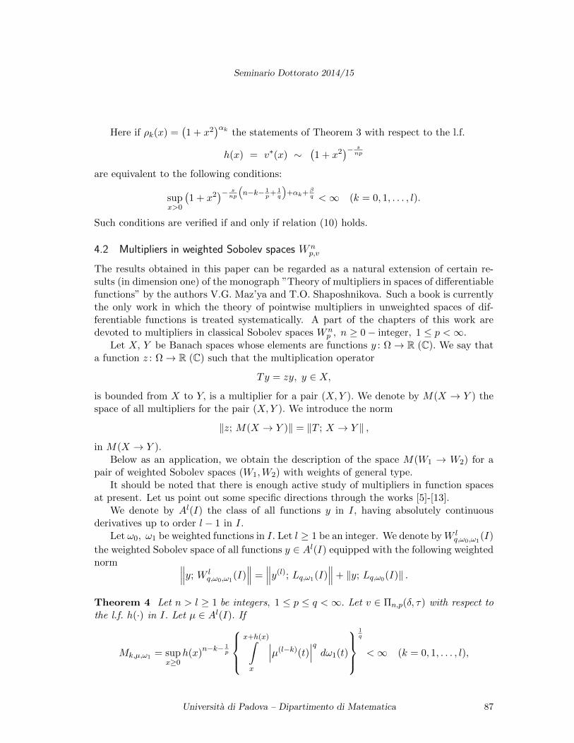
Seminario Dottorato 2014/15
Here if ρk(x) =(1 + x2
)αk the statements of Theorem 3 with respect to the l.f.
h(x) = v∗(x) ∼(1 + x2
)− snp
are equivalent to the following conditions:
supx>0
(1 + x2
)− snp
(n−k− 1
p+ 1q
)+αk+β
q <∞ (k = 0, 1, . . . , l).
Such conditions are verified if and only if relation (10) holds.
4.2 Multipliers in weighted Sobolev spaces W np,v
The results obtained in this paper can be regarded as a natural extension of certain re-sults (in dimension one) of the monograph ”Theory of multipliers in spaces of differentiablefunctions” by the authors V.G. Maz’ya and T.O. Shaposhnikova. Such a book is currentlythe only work in which the theory of pointwise multipliers in unweighted spaces of dif-ferentiable functions is treated systematically. A part of the chapters of this work aredevoted to multipliers in classical Sobolev spaces Wn
p , n ≥ 0− integer, 1 ≤ p <∞.Let X, Y be Banach spaces whose elements are functions y : Ω→ R (C). We say that
a function z : Ω→ R (C) such that the multiplication operator
Ty = zy, y ∈ X,
is bounded from X to Y, is a multiplier for a pair (X,Y ). We denote by M(X → Y ) thespace of all multipliers for the pair (X,Y ). We introduce the norm
‖z; M(X → Y )‖ = ‖T ; X → Y ‖ ,
in M(X → Y ).Below as an application, we obtain the description of the space M(W1 → W2) for a
pair of weighted Sobolev spaces (W1,W2) with weights of general type.It should be noted that there is enough active study of multipliers in function spaces
at present. Let us point out some specific directions through the works [5]-[13].We denote by Al(I) the class of all functions y in I, having absolutely continuous
derivatives up to order l − 1 in I.Let ω0, ω1 be weighted functions in I. Let l ≥ 1 be an integer. We denote byW l
q,ω0,ω1(I)
the weighted Sobolev space of all functions y ∈ Al(I) equipped with the following weightednorm ∥∥∥y; W l
q,ω0,ω1(I)∥∥∥ =
∥∥∥y(l); Lq,ω1(I)∥∥∥+ ‖y; Lq,ω0(I)‖ .
Theorem 4 Let n > l ≥ 1 be integers, 1 ≤ p ≤ q <∞. Let v ∈ Πn,p(δ, τ) with respect tothe l.f. h(·) in I. Let µ ∈ Al(I). If
Mk,µ,ω1 = supx≥0
h(x)n−k− 1
p
x+h(x)∫x
∣∣∣µ(l−k)(t)∣∣∣q dω1(t)
1q
<∞ (k = 0, 1, . . . , l),
Universita di Padova – Dipartimento di Matematica 87
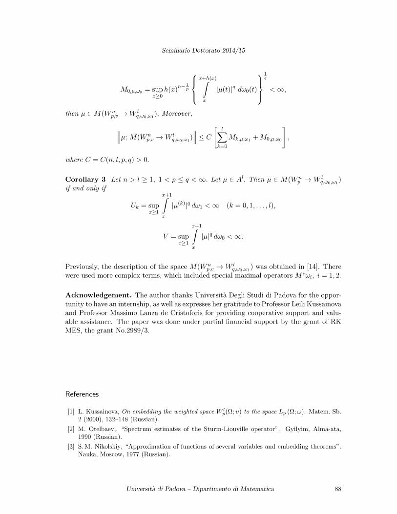
Seminario Dottorato 2014/15
M0,µ,ω0 = supx≥0
h(x)n− 1
p
x+h(x)∫x
|µ(t)|q dω0(t)
1q
<∞,
then µ ∈M(Wnp,v →W l
q,ω0,ω1). Moreover,
∥∥∥µ; M(Wnp,v →W l
q,ω0,ω1)∥∥∥ ≤ C [ l∑
k=0
Mk,µ,ω1 +M0,µ,ω0
],
where C = C(n, l, p, q) > 0.
Corollary 3 Let n > l ≥ 1, 1 < p ≤ q < ∞. Let µ ∈ Al. Then µ ∈ M(Wnp → W l
q,ω0,ω1)
if and only if
Uk = supx≥1
x+1∫x
|µ(k)|q dω1 <∞ (k = 0, 1, . . . , l),
V = supx≥1
x+1∫x
|µ|q dω0 <∞.
Previously, the description of the space M(Wnp,v → W l
q,ω0,ω1) was obtained in [14]. There
were used more complex terms, which included special maximal operators M∗ωi, i = 1, 2.
Acknowledgement. The author thanks Universita Degli Studi di Padova for the oppor-tunity to have an internship, as well as expresses her gratitude to Professor Leili Kussainovaand Professor Massimo Lanza de Cristoforis for providing cooperative support and valu-able assistance. The paper was done under partial financial support by the grant of RKMES, the grant No.2989/3.
References
[1] L. Kussainova, On embedding the weighted space W lp(Ω; υ) to the space Lp (Ω;ω). Matem. Sb.
2 (2000), 132–148 (Russian).
[2] M. Otelbaev,, “Spectrum estimates of the Sturm-Liouville operator”. Gyilyim, Alma-ata,1990 (Russian).
[3] S. M. Nikolskiy, “Approximation of functions of several variables and embedding theorems”.Nauka, Moscow, 1977 (Russian).
Universita di Padova – Dipartimento di Matematica 88
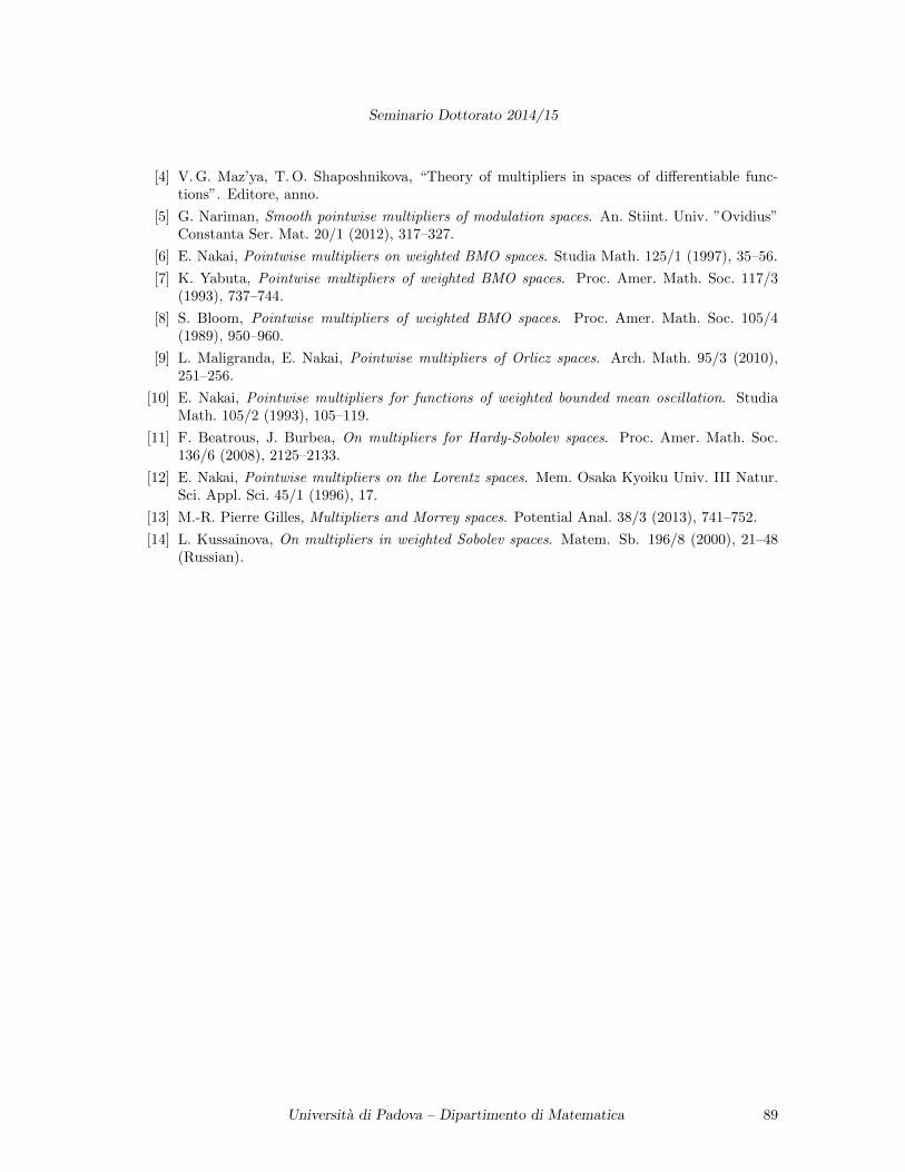
Seminario Dottorato 2014/15
[4] V. G. Maz’ya, T. O. Shaposhnikova, “Theory of multipliers in spaces of differentiable func-tions”. Editore, anno.
[5] G. Nariman, Smooth pointwise multipliers of modulation spaces. An. Stiint. Univ. ”Ovidius”Constanta Ser. Mat. 20/1 (2012), 317–327.
[6] E. Nakai, Pointwise multipliers on weighted BMO spaces. Studia Math. 125/1 (1997), 35–56.
[7] K. Yabuta, Pointwise multipliers of weighted BMO spaces. Proc. Amer. Math. Soc. 117/3(1993), 737–744.
[8] S. Bloom, Pointwise multipliers of weighted BMO spaces. Proc. Amer. Math. Soc. 105/4(1989), 950–960.
[9] L. Maligranda, E. Nakai, Pointwise multipliers of Orlicz spaces. Arch. Math. 95/3 (2010),251–256.
[10] E. Nakai, Pointwise multipliers for functions of weighted bounded mean oscillation. StudiaMath. 105/2 (1993), 105–119.
[11] F. Beatrous, J. Burbea, On multipliers for Hardy-Sobolev spaces. Proc. Amer. Math. Soc.136/6 (2008), 2125–2133.
[12] E. Nakai, Pointwise multipliers on the Lorentz spaces. Mem. Osaka Kyoiku Univ. III Natur.Sci. Appl. Sci. 45/1 (1996), 17.
[13] M.-R. Pierre Gilles, Multipliers and Morrey spaces. Potential Anal. 38/3 (2013), 741–752.
[14] L. Kussainova, On multipliers in weighted Sobolev spaces. Matem. Sb. 196/8 (2000), 21–48(Russian).
Universita di Padova – Dipartimento di Matematica 89
Seminario Dottorato 2014/15
Preferences in AI
Cristina Cornelio (∗)
Abstract. Artificial Intelligence (AI) is a field that has a long history but still constantly andactively growing and changing. The applications of AI are several, for example web search, speechrecognition, face recognition, machine translation, autonomous driving, automatic scheduling etc.These are all complex real-world problems, and the goal of artificial intelligence is to tackle themwith rigorous mathematical tools: machine learning, search, game playing, Markov decision pro-cesses, constraint satisfaction, graphical models, and logic. Recently, a new concept became veryimportant in AI: the use of preferences. Let’s think about social networks, online shops, systemsthat suggest music or films. In this document it is presented an overview on the main formalismsof qualitative preferences in AI, a particular subset of models to represent preferences, very usefulin real word applications.
1 Artificial Intelligence: an overview
Artificial Intelligence (AI) is a big field and there are many important applications of AItechnology in the real world. Most important are:
• Robotics. Robotics is widely used in industrial automation, but they are also usedas medical surgery support to help doctors in complicated surgical procedures. Arti-ficial body components (arms, legs) and also artificial organs (heart) was developedto interact directly with the human brain. Robotics is widely used in space explo-ration or to develop exploration robots for difficult conditions, for example with toohight/low temperature or pressure (e.g. deep sea).
• Natural language processing. The goal of this subfield is the direct interactionhuman-machines. A machine has to understand a text and to make a summary, totranslate a text in a proper way, to recognize if two texts are written by the sameperson, or to search text following the meaning and not following only the words inthe name.
• Autonomous control systems and planning. Autonomous schedule and plan-ning is mainly useful for robotic application (e.g. industrial robot and managementof the production line), but also in control system. Let’s think about the electricity
(∗)Ph.D. course, Universita di Padova, Dip. Matematica, via Trieste 63, I-35121 Padova, Italy; E-mail:. Seminar held on April 29th, 2015.
Universita di Padova – Dipartimento di Matematica 90
Seminario Dottorato 2014/15
industries: Enel uses neural networks to manage the electricity switches betweenthe centrals, the amount of produced energy and the temperature of the areas ofproduction. This subfield is also used to solve conflicts with the instructions givenby different machines/sensors.
• Games. IBM’s Deep Blue became the first computer program that wins again theworld chess champion Garry Kasparov. Let’s think about the video-games market:video-games are becoming increasingly realistic using AI components.
• Machine Learning. Machine Learning is a system that improves its performanceon a particular task using past experience. Examples of machine learning applicationare auto-parking cars , driver-less cars (e.g. Google car), handwriting recognitionand speech recognition.
• Preferences. Preferences play an increasing role in the web application. Recom-mender systems are hidden behind many web sites (e.g. Amazon or Netflix) tosuggest music, films, or products.
2 Qualitative Preferences on combinatorial domains
The ability to express preferences in a faithful way, which can be handled efficiently, isessential in many reasoning tasks. In settings such as e-commerce, on demand video,and other settings where supply outstrips an individuals ability to view all the availablechoices, we require an efficient formalism to model and reason with complex, interdepen-dent preferences. We may also use these preferences to make decisions about joint plans,actions, or items in multi-agent environments. Agents express their preferences over a setof candidate decisions, these preferences are aggregated into one decision which satisfies asmany agents as possible. Often multi-attribute preference modeling and reasoning causesa combinatorial explosion. The set of candidates is often described as a product of mul-tiple features, for example, a users preferences over a set of cars, which can be describedby their colors, technical specifications, cost, reliability, etc. A number of compact rep-resentation languages have been developed in the literature to tackle the computationalchallenges arising from these problems. The main tool for representing and reasoning withconditional preference statements of a single agent are the CP-nets. A more general andcomplete version of CP-nets are the GCP-nets, introduced in the following section (Sec-tion 3). Then we will introduce the other main formulations of qualitative preferences oncombinatorial domains.
3 GCP-nets
GCP-nets ([7] and [6]) allow a general form of conditional and qualitative preferences tobe modeled compactly.
Definition 3.1 A Generalized CP-net (GCP-net) C over Var is a set of conditionalpreference rules. A conditional preference rule is an expression p : l > l, where l is
Universita di Padova – Dipartimento di Matematica 91
Seminario Dottorato 2014/15
a literal of some atom X ∈ Var and p is a propositional formula over Var that does notinvolve variable X. A GCP-net corresponds to a directed graph (dependency graph) whereeach node is associated with a feature and the edges are pairs (Y,X) where Y appears inp in some rule p : x > x or p : x > x. Each node X is associated with a CP-table whichexpresses the user preference over the values of X. Each row of the CP-table correspondsto a conditional preference rule.
The CP-tables of a GCP-net can be incomplete (i.e. for some values of some variables’parents, the preferred value of X may not be specified) and/or locally inconsistent (i.e.for some values of some variables’ parents, the table may both contain the informationx > x and x > x). CP-nets [2] are a special case of GCP-net in which the preferences arelocally consistent and locally complete.
An outcome in a GCP-net is a complete assignment to all features. For example, givenVar = X1, X2 and binary domains D1 = D2 = T, F, all the possible outcomes areTT , TF , FT and FF .
A worsening flip is a change in the value of a feature to a value which is less preferredaccording to the cp-statement for that feature. This concept defines an order over the setof outcomes such that one outcome o is preferred to another outcome o′ (o o′) if and onlyif there is a chain of worsening flips from o to o′. The notion of worsening flip induces apreorder over the set of outcomes. This preorder allows maximal elements that correspondto the so-called optimal outcomes, which are outcomes that have no other outcome betterthan them.
Given any GCP-net and CP-net the problems of consistency checking and findingoptimal outcomes are PSPACE-complete [7]. Moreover, there could be several differentmaximal elements. When the dependency graph has no cycle the CP-net is called acyclic.The optimal outcomes for such nets are unique and can be found in polynomial time in N .The procedure used to this purpose is usually called a sweep forward and takes N steps[2].
The problem of dominance testing (i.e. determining if one outcome is preferred toanother) is PSPACE-complete for both GCP-nets and CP-nets. It is polynomial if theCP-nets are tree structured or poly-tree structured [5, 7].
4 CP-nets
CP-nets are a graphical model for compactly representing conditional and qualitative pref-erence relations [2]. They exploit conditional preferential independence by decomposing anagent’s preferences via the ceteris paribus (cp) assumption (all other things being equal).
CP-nets correspond to complete and locally consistent GCP-nets.CP-nets bear some similarity to Bayesian networks [4]: both use directed graphs where
each node stands for a domain variable, and assume a set of features F = X1, . . . , Xnwith finite domains D1, . . . , Dn.
Definition 4.1 A CP-net (conditional preference network) over features F = X1, . . . , Xnwith finite domains D1, . . . , Dn is a direct graph G over F in which:
Universita di Padova – Dipartimento di Matematica 92
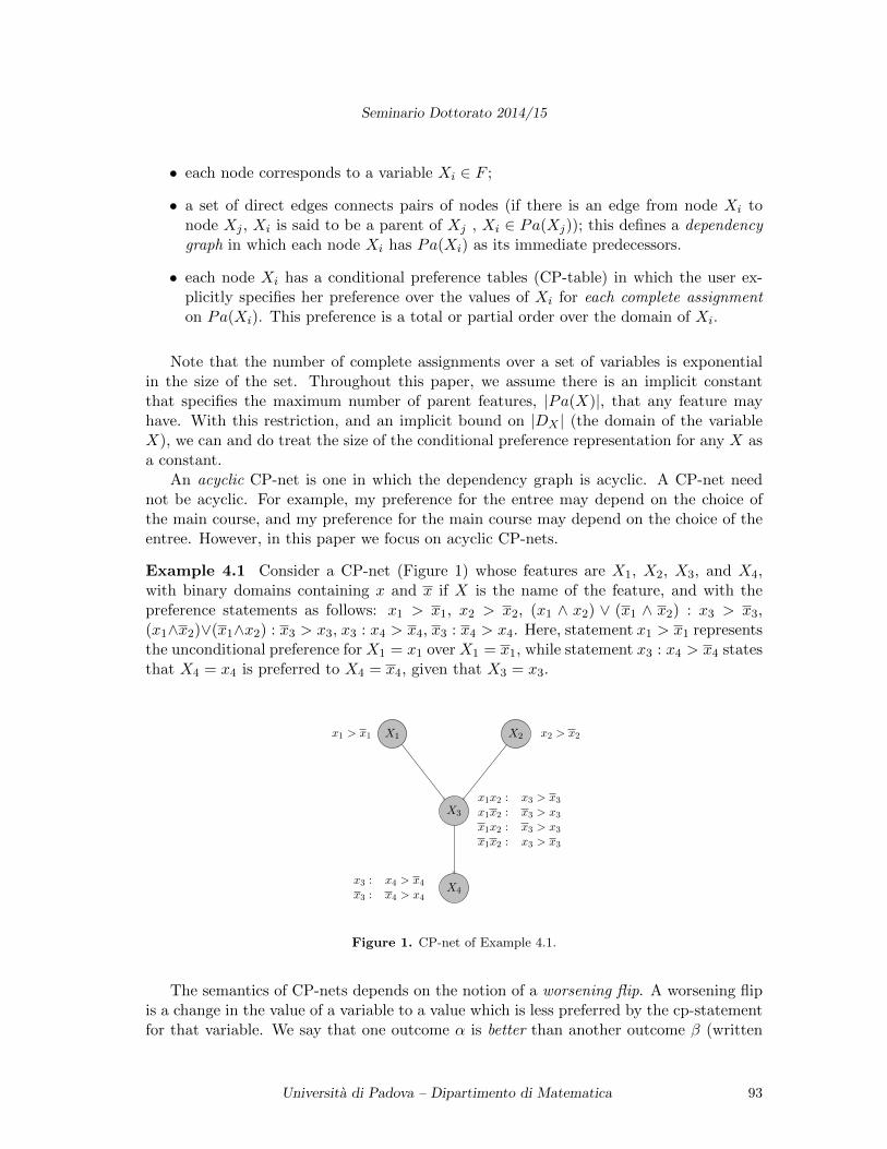
Seminario Dottorato 2014/15
• each node corresponds to a variable Xi ∈ F ;
• a set of direct edges connects pairs of nodes (if there is an edge from node Xi tonode Xj , Xi is said to be a parent of Xj , Xi ∈ Pa(Xj)); this defines a dependencygraph in which each node Xi has Pa(Xi) as its immediate predecessors.
• each node Xi has a conditional preference tables (CP-table) in which the user ex-plicitly specifies her preference over the values of Xi for each complete assignmenton Pa(Xi). This preference is a total or partial order over the domain of Xi.
Note that the number of complete assignments over a set of variables is exponentialin the size of the set. Throughout this paper, we assume there is an implicit constantthat specifies the maximum number of parent features, |Pa(X)|, that any feature mayhave. With this restriction, and an implicit bound on |DX | (the domain of the variableX), we can and do treat the size of the conditional preference representation for any X asa constant.
An acyclic CP-net is one in which the dependency graph is acyclic. A CP-net neednot be acyclic. For example, my preference for the entree may depend on the choice ofthe main course, and my preference for the main course may depend on the choice of theentree. However, in this paper we focus on acyclic CP-nets.
Example 4.1 Consider a CP-net (Figure 1) whose features are X1, X2, X3, and X4,with binary domains containing x and x if X is the name of the feature, and with thepreference statements as follows: x1 > x1, x2 > x2, (x1 ∧ x2) ∨ (x1 ∧ x2) : x3 > x3,(x1∧x2)∨(x1∧x2) : x3 > x3, x3 : x4 > x4, x3 : x4 > x4. Here, statement x1 > x1 representsthe unconditional preference for X1 = x1 over X1 = x1, while statement x3 : x4 > x4 statesthat X4 = x4 is preferred to X4 = x4, given that X3 = x3.
X1 X2
X3
X4
x1 > x1 x2 > x2
x1x2 : x3 > x3
x1x2 : x3 > x3
x1x2 : x3 > x3
x1x2 : x3 > x3
x3 : x4 > x4
x3 : x4 > x4
Figure 1. CP-net of Example 4.1.
The semantics of CP-nets depends on the notion of a worsening flip. A worsening flipis a change in the value of a variable to a value which is less preferred by the cp-statementfor that variable. We say that one outcome α is better than another outcome β (written
Universita di Padova – Dipartimento di Matematica 93
Seminario Dottorato 2014/15
α > β) if and only if there is a chain of worsening flips from α to β. This definition inducesa preorder over the outcomes.
In general, finding optimal outcomes and testing for optimality in this ordering is NP-hard. However, in acyclic CP-nets, there is only one optimal outcome and this can befound in as many steps as the number of features via a sweep forward procedure [2]. Wesweep through the CP-net, following the arrows in the dependency graph and assigningat each step the most preferred value in the preference table. More formally:
Definition 4.2 The sweep forward procedure, in acyclic CP-nets, to achieve the optimalvalue is as follows:
• Step 0 : We choose for the CP-nets independent features the value that it is rankedfirst in the ordering of the domains values.
• Step i : For each feature that it is not yet assigned and that has the values assign-ments of all the parents, we choose the value that it is most preferred (so ranked first)in the ordering of the domains values (in the rows corresponding to that particularassignments for the parentss values).
Example 4.2 For instance, in the CP-net above (Example 4.1), we would choose X1 = x1
and X2 = x2, then, because the parents X1X2 = x1x2, we choose X3 = x3 and then,because X3 = x3 we obtain X4 = x4. The optimal outcome is therefore x1x2x3x4.
Each step in the sweep forward procedure is exponential in the number of parents ofthe current feature, and there are as many steps as features. In this paper we assume thenumber of parents is bounded, so this algorithm takes time polynomial in the size of theCP-net.
In the general case the optimal outcome coincides with the solutions of a constraintproblem obtained replacing each cp-statement with a constraint. For example, the follow-ing cp-statement (concerning the Example 4.1) (x1 ∧ x2) ∨ (x1 ∧ x2) : x3 > x3 would bereplaced by the constraint (x1 ∧ x2) ∨ (x1 ∧ x2)⇒ x3 > x3.
Determining if one outcome is better than another according to this ordering (calleda dominance query) is NP-hard even for acyclic CP-nets [5, 7]. Whilst tractable specialcases exist, there are also acyclic CP-nets in which there are exponentially long chains ofworsening flips between two outcomes.
Example 4.3 In the CP-net of the Example 4.1, x1x2x3x4 is worse than x1x2x3x4.
4.1 Variants of CP-nets
CP-nets are deeply studied and widely used, thus many variants and generalization wasdeveloped. The main are the following:
• TCP-nets (Tradeoffs-enhanced CP-nets) [3] are a extension of CP-net that permitsto represent also the notion of relative importance and conditional relative impor-tance. A variable X is relative more important respect to a variable Y (X B Y ) if
Universita di Padova – Dipartimento di Matematica 94
Seminario Dottorato 2014/15
the it is more important that the value of X be high than that the value of Y behigh. For instance “The length of the journey is more important to me than thechoice of airline”. A variable X is relative more important respect to a variable Ygiven an assignment of a variable Z (Z = z0 : X B Y,Z = z1 : Y B X) if the itis more important that the value of X be high than that the value of Y be high,given the evidence that Z = z0. For instance “The length of the journey is moreimportant to me than the choice of airline provided that I am lecturing the followingday. Otherwise the choice of airline is more important”. This formulation introducethe CI-tables (conditional importance tables) to the dependency graph, to expressthe conditional importance statements.
• UCP-nets (Utility Conditional Preference networks) [1] are an extension of CP-nets in which the preferences are expressed in a quantitative formulation, and notonly qualitative as in CP-nets. Each varible express the preferences of the user ina table that contains the user utility values of the values in the variable domain. ACP-statement of the form x : y > y is represented in UCP-net by fY (y|x) = u1,fY (y|x) = u2 and u1 > u2 where fY is the utility function of the variable Y .
• mCP-nets (multi-agent Conditional Preference networks) [8] are an extension ofCP-net formalism to model and handle the preferences of multiple agents. A mCP-net is a set of m partial CP-nets (CP-net with partial or missing information) whichcan share some features. A mCP-net dependency graph is obtained by combiningthe graphs of the partial of the parial CP-nets having one occurrence of each sharedfeature. A feature can be shared between the CP-nets, visible to other CP-nets thatcan use this feature as precondition in the CP-statements, or private if is ranked inonly one CP-net and is not visible to the other CP-nets.
5 CP-theories and Comparative Preference languages
Other important generalizations of CP-nets are CP-theories and comparative preferencelanguages, two different logic formulation of qualitative preferences. The correspondingtheories and languages are defined below.
5.1 CP-theories
CP-theories are introduced in [9] as a logic of conditional preference which generalizesCP-nets.
Definition 5.1 Given a set of variables Var = X1, · · · , XN with domains Di, i =1, . . . , n, the language LVar is defined by all the statements of the form: u : xi x′i[W ]where u is an assignment of a set of variables U ⊆ Var \ Xi, xi 6= x′i ∈ Di and W is aset of variables such that W ⊆ (Var \ U \ Xi).
Definition 5.2 Given a language LVar as defined above, a conditional preference theory(CP-theory) Γ on Var is a subset of LVar . Γ generates a set of preferences that cor-
Universita di Padova – Dipartimento di Matematica 95
Seminario Dottorato 2014/15
responds to the set Γ∗ =⋃ϕ∈Γ ϕ
∗ where given ϕ = u : xi x′i[W ], ϕ∗ is defined asϕ∗ = (tuxw, tux′w′) : t ∈ Var \ (Xi ∪ U ∪W), w, w′ ∈W.
A CP-net is a particular case of a CP-theory where W = ∅ for all ϕ ∈ Γ.Two graphs are associated to a CP-theory: H(Γ) = (Xj , Xi)|∃ϕ ∈ Γ s.t. ϕ = u : xi
x′i[W ] and Xj ∈ U and G(Γ) = H ∪ (Xi, Xj)|∃ϕ ∈ Γ s.t. ϕ = u : xi x′i[W ] and Xj ∈W.
The semantics of CP-theories depends on the notion of a worsening swap, which is achange in the assignment of a set of variables to an assignment which is less preferred bya rule ϕ ∈ Γ. We say that one outcome o is better than another outcome o′ (o o′) if andonly if there is a chain of worsening swaps (a worsening swapping sequence) from o to o′.
Definition 5.3 A CP-theory Γ is locally consistent if and only if for all Xi ∈ Var andu ∈ Pa(Xi) in the graph H(Γ), Xiu is irreflexive.
Local consistency can be determined in time proportional to |Γ|2N . Given a CP-theoryΓ, if the graph G(Γ) is acyclic, Γ is consistent if and only if Γ is locally consistent, thusglobal consistency has the same complexity as local consistency given an acyclic graphG(Γ).
5.2 Comparative Preference languages
Comparative Preference theories [10] are an extension of CP-theories.
Definition 5.4 The comparative preference language CLVar is defined by all statementsof the form: p > q||T where P , Q and T are subsets of Var and p and q are assignmentsrespectively of the variables in P and in Q.
Definition 5.5 Given a language CLVar as defined above, a comparative preference theoryΛ on Var is a subset of CLVar . Λ generates a set of preferences that corresponds to theset Λ∗ =
⋃ϕ∈Λ ϕ
∗ where if ϕ = p > q||T , ϕ∗ is defined as a pair (α, β) of outcomes suchthat α extends p and β extends q and α and β agree on T : α T= β T .
References
[1] C. Boutilier, F. Bacchus, and R. I. Brafman, Ucp-networks: A directed graphical rep- resenta-tion of conditional utilities. In UAI ?01: Proceedings of the 17th Conference in Uncertaintyin Artificial Intelligence, University of Washington, Seattle, Washington, USA, August 2-5,2001, pages 56?64, 2001.
[2] C. Boutilier, R. Brafman, C. Domshlak, H. Hoos, and D. Poole, CP-nets: A tool for represent-ing and reasoning with conditional ceteris paribus preference statements. Journal of ArtificialIntelligence Research 21 (2004), 135–191.
Universita di Padova – Dipartimento di Matematica 96
Seminario Dottorato 2014/15
[3] R. Brafman and C. Domshlak, Introducing variable importance tradeoffs into cp-nets. In UAI?02, pages 69–76, 2002.
[4] B. D?Ambrosio, Inference in bayesian networks. AI Magazine, 20(2):21, 1999.
[5] C. Domshlak and R. Brafman, CP-nets: Reasoning and consistency testing. In Proc. 8thInternational Conference on Principles of Knowledge Representation and Reasoning (KR),2002.
[6] C. Domshlak, F. Rossi, K. Venable, and T. Walsh, Reasoning about soft constraints andconditional preferences: complexity results and approximation techniques. In Proc. of the18th International Joint Conference on Artificial Intelligence (IJCAI), 2003.
[7] J. Goldsmith, J. Lang, M. Truszczynski, and N. Wilson, The Computational Com- plexityof Dominance and Consistency in CP-nets. Journal of Artificial Intelligence Research 33/1(2008), 403–432.
[8] F. Rossi, K. Venable, and T. Walsh, mCP nets: representing and reasoning with preferencesof multiple agents. In Proc. of the 19th AAAI Conference on Artificial Intelligence (AAAI),2004.
[9] N. Wilson, Extending CP-Nets with Stronger Conditional Preference Statements. In Proceed-ings of AAAI-04, pages 735–741, 2004.
[10] N. Wilson, Efficient Inference for Expressive Comparative Preference Languages. In Proceed-ings of IJCAI-09, 2009.
Universita di Padova – Dipartimento di Matematica 97
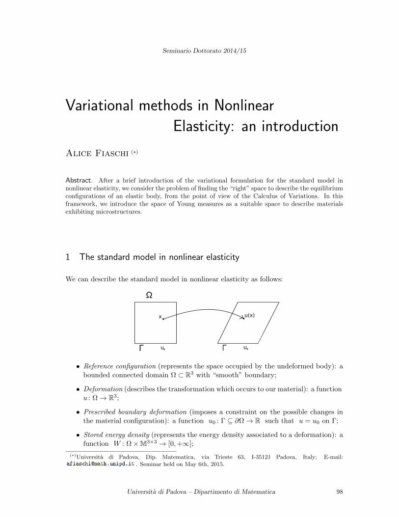
Seminario Dottorato 2014/15
Variational methods in Nonlinear
Elasticity: an introduction
Alice Fiaschi (∗)
Abstract. After a brief introduction of the variational formulation for the standard model innonlinear elasticity, we consider the problem of finding the “right” space to describe the equilibriumconfigurations of an elastic body, from the point of view of the Calculus of Variations. In thisframework, we introduce the space of Young measures as a suitable space to describe materialsexhibiting microstructures.
1 The standard model in nonlinear elasticity
We can describe the standard model in nonlinear elasticity as follows:
x u(x)
u0 u0
Ω
Γ
• Reference configuration (represents the space occupied by the undeformed body): abounded connected domain Ω ⊂ R3 with “smooth” boundary;
• Deformation (describes the transformation which occurs to our material): a functionu : Ω→ R3;
• Prescribed boundary deformation (imposes a constraint on the possible changes inthe material configuration): a function u0 : Γ ⊆ ∂Ω→ R such that u = u0 on Γ;
• Stored energy density (represents the energy density associated to a deformation): afunction W : Ω×M3×3 → [0,+∞];
(∗)Universita di Padova, Dip. Matematica, via Trieste 63, I-35121 Padova, Italy; E-mail:. Seminar held on May 6th, 2015.
Universita di Padova – Dipartimento di Matematica 98
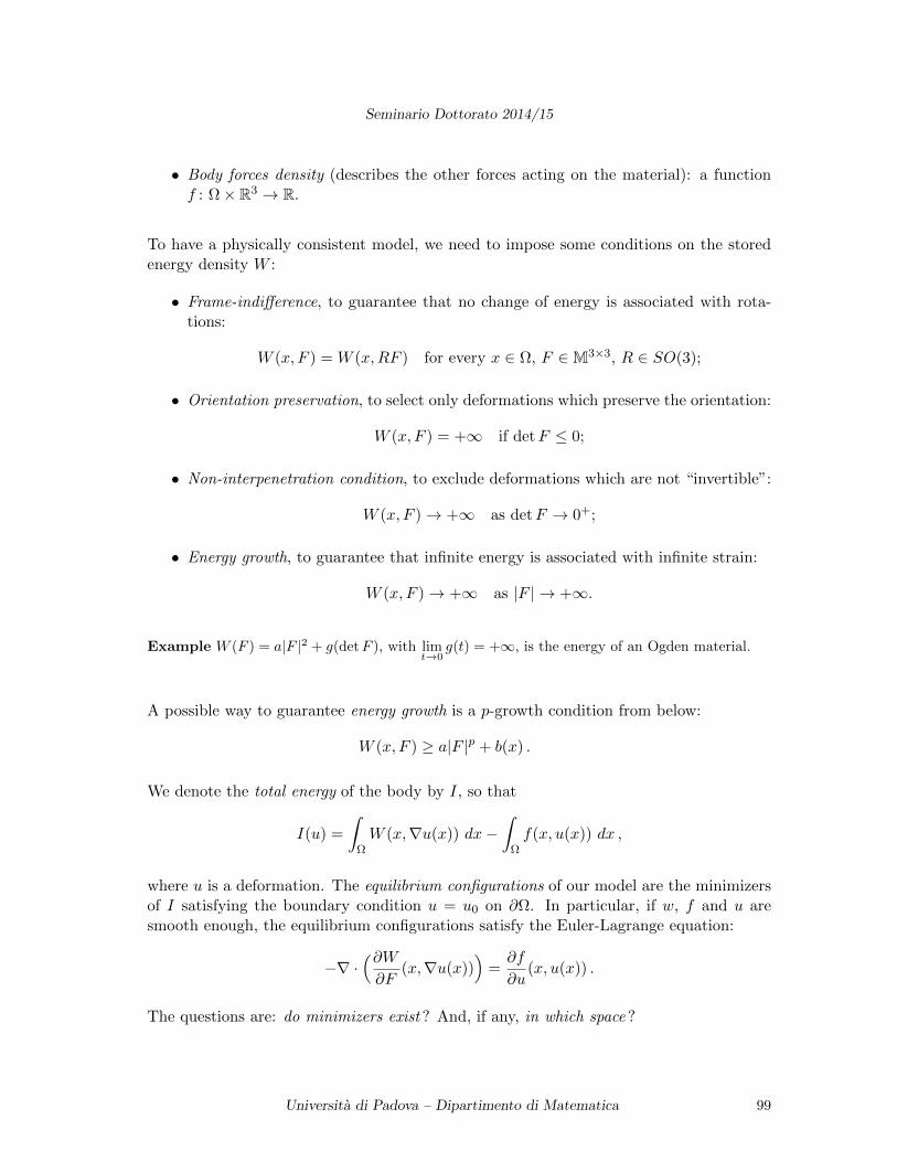
Seminario Dottorato 2014/15
• Body forces density (describes the other forces acting on the material): a functionf : Ω× R3 → R.
To have a physically consistent model, we need to impose some conditions on the storedenergy density W :
• Frame-indifference, to guarantee that no change of energy is associated with rota-tions:
W (x, F ) = W (x,RF ) for every x ∈ Ω, F ∈M3×3, R ∈ SO(3);
• Orientation preservation, to select only deformations which preserve the orientation:
W (x, F ) = +∞ if detF ≤ 0;
• Non-interpenetration condition, to exclude deformations which are not “invertible”:
W (x, F )→ +∞ as detF → 0+;
• Energy growth, to guarantee that infinite energy is associated with infinite strain:
W (x, F )→ +∞ as |F | → +∞.
Example W (F ) = a|F |2 + g(detF ), with limt→0
g(t) = +∞, is the energy of an Ogden material.
A possible way to guarantee energy growth is a p-growth condition from below:
W (x, F ) ≥ a|F |p + b(x) .
We denote the total energy of the body by I, so that
I(u) =
∫ΩW (x,∇u(x)) dx−
∫Ωf(x, u(x)) dx ,
where u is a deformation. The equilibrium configurations of our model are the minimizersof I satisfying the boundary condition u = u0 on ∂Ω. In particular, if w, f and u aresmooth enough, the equilibrium configurations satisfy the Euler-Lagrange equation:
−∇ ·(∂W∂F
(x,∇u(x)))
=∂f
∂u(x, u(x)) .
The questions are: do minimizers exist ? And, if any, in which space ?
Universita di Padova – Dipartimento di Matematica 99
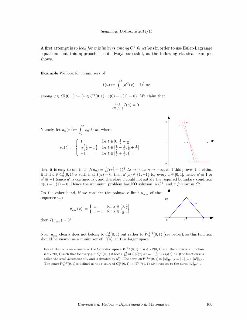
Seminario Dottorato 2014/15
A first attempt is to look for minimizers among C2 functions in order to use Euler-Lagrangeequation: but this approach is not always sucessful, as the following classical exampleshows.
Example We look for minimizers of
I(u) :=
∫ 1
0
(u′2(x)− 1)2 dx
among u ∈ C10 (0, 1) := u ∈ C1(0, 1), u(0) = u(1) = 0. We claim that
infC1
0 (0,1)I(u) = 0 .
Namely, let un(x) :=
∫ x
0
vn(t) dt, where
vn(t) :=
1 for t ∈ [0, 12 −
1n ]
n(
12 − x
)for t ∈ [ 12 −
1n ,
12 + 1
n ]
−1 for t ∈ [ 12 + 1n , 1] :
0
1
-1
1/2 1
vn
v4
then it is easy to see that I(un) =∫ 1
0(v2n − 1)2 dx → 0 as n → +∞, and this proves the claim.
But if u ∈ C10 (0, 1) is such that I(u) = 0, then u′(x) ∈ 1,−1 for every x ∈ [0, 1], hence u′ ≡ 1 or
u′ ≡ −1 (since u′ is continuous), and therefore u could not satisfy the required boundary conditionu(0) = u(1) = 0. Hence the minimum problem has NO solution in C1, and a fortiori in C2.
On the other hand, if we consider the pointwise limit umin
of thesequence un:
umin
(x) :=
x for x ∈ [0, 12 ]1− x for x ∈ [ 12 , 1]
then I(umin
) = 0 !
1/2
0 1/2 1
um
Now, umin
clearly does not belong to C10 (0, 1) but rather to W 1,4
0 (0, 1) (see below), so this functionshould be viewed as a minimizer of I(u) in this larger space.
Recall that u is an element of the Sobolev space W 1,p(0, 1) if u ∈ Lp(0, 1) and there exists a function
v ∈ Lp(0, 1) such that for every φ ∈ C∞c (0, 1) it holds∫ 10 u(x)φ′(x) dx = −
∫ 10 v(x)φ(x) dx (the function v is
called the weak derivative of u and is denoted by u′). The norm on W 1,p(0, 1) is ‖u‖W1,p = ‖u‖Lp +‖u′‖Lp .
The space W 1,p0 (0, 1) is defined as the closure of C∞0 (0, 1) in W 1,p(0, 1) with respect to the norm ‖u‖W1,p .
Universita di Padova – Dipartimento di Matematica 100
Seminario Dottorato 2014/15
The weak derivative of umin
is vmin
(x) :=
1 for x ∈ [0, 12 )−1 for x ∈ ( 1
2 , 1]: indeed
∫ 1
0
umin
(x)φ′(x) dx =
∫ 12
0
xφ′(x) dx+
∫ 1
12
(1− x)φ′(x) dx
=[xφ(x)
]1/20−∫ 1
2
0
φ(x) dx+[(1− x)φ(x)
]112
−∫ 1
12
(−1)φ(x) dx
=1
2φ( 1
2 )−(
1− 12
)φ( 1
2 )−∫ 1
0
vmin
(x)φ(x) dx = −∫ 1
0
vmin
(x)φ(x) dx .
Hence umin∈W 1,4(0, 1) and I(u
min) =
∫ 1
0(v
min(x)2 − 1) dx = 0 , as claimed.
2 The Direct Method of the Calculus of Variations
The previous example is in fact an instance of a more general situation.
Theorem (Existence Theorem) Let p > 1, and let W : Ω × R3 ×M3×3 → [0,+∞] be acontinuous map such that
• W (x, u, F ) ≥ a|F |p + b|u|q + c(x), for a > 0, b ∈ R, c ∈ L1(Ω), 1 ≤ q < p (coer-civeness);
• the map F 7→W (x, u, F ) is convex (convexity).
Then there exists (at least) one minimizer of I(u) =∫
ΩW (x, u(x),∇u(x)) dx in u0 +
W 1,p0 (Ω), provided I(u0) < +∞.
A minimizing sequence is a sequence un ∈ u0 +W 1,p0 (Ω) with I(un)→ inf I.
We just give an idea of the proof of the existence theorem:
• coerciveness implies the compactness of a minimizing sequence in the weak topologyof W 1,p, hence unk u for some subsequence (unk)k;
• convexity implies the lower semicontinuity of I with respect to the weak topology ofW 1,p, hence I(u) ≤ lim inf I(unk) = inf I.
The point is rather that the hypothesis of convexity is incompatible with our physicalassumptions on W , as the following simple example shows.
Example Recall that among our physical assumptions we required that W (RF ) = W (F ) for everyR ∈ SO(3), and that W (F ) → +∞ if detF → 0. Now, for simplicity let us consider F ∈ M2×2
and suppose W (1) < +∞. Let R =
(cosα − sinαsinα cosα
). Since 1
2R + 12R
T = (cosα)1, convexity
implies that W ((cosα)1) ≤ 12W (R) + 1
2W (RT ) = W (1)< +∞; but for α→ π2 , det((cosα)1)→ 0
although W ((cosα)1) is bounded from above by W (1) < +∞.
Universita di Padova – Dipartimento di Matematica 101
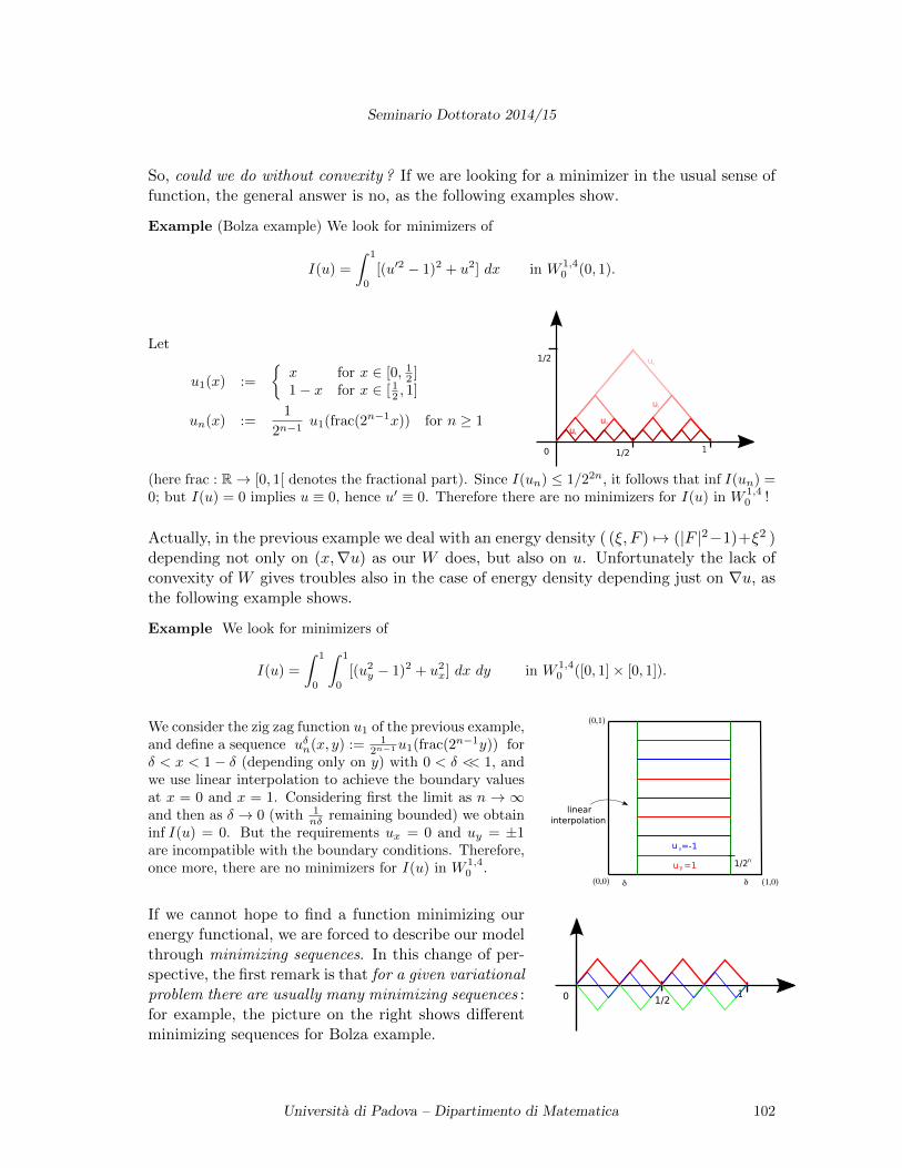
Seminario Dottorato 2014/15
So, could we do without convexity ? If we are looking for a minimizer in the usual sense offunction, the general answer is no, as the following examples show.
Example (Bolza example) We look for minimizers of
I(u) =
∫ 1
0
[(u′2 − 1)2 + u2] dx in W 1,40 (0, 1).
Let
u1(x) :=
x for x ∈ [0, 12 ]1− x for x ∈ [ 12 , 1]
un(x) :=1
2n−1u1(frac(2n−1x)) for n ≥ 1
1/2
0 1/2 1
u
1
2
3
4
u
u
u
(here frac : R→ [0, 1[ denotes the fractional part). Since I(un) ≤ 1/22n, it follows that inf I(un) =0; but I(u) = 0 implies u ≡ 0, hence u′ ≡ 0. Therefore there are no minimizers for I(u) in W 1,4
0 !
Actually, in the previous example we deal with an energy density ( (ξ, F ) 7→ (|F |2−1)+ξ2 )depending not only on (x,∇u) as our W does, but also on u. Unfortunately the lack ofconvexity of W gives troubles also in the case of energy density depending just on ∇u, asthe following example shows.
Example We look for minimizers of
I(u) =
∫ 1
0
∫ 1
0
[(u2y − 1)2 + u2x] dx dy in W 1,40 ([0, 1]× [0, 1]).
We consider the zig zag function u1 of the previous example,and define a sequence uδn(x, y) := 1
2n−1u1(frac(2n−1y)) forδ < x < 1− δ (depending only on y) with 0 < δ << 1, andwe use linear interpolation to achieve the boundary valuesat x = 0 and x = 1. Considering first the limit as n → ∞and then as δ → 0 (with 1
nδ remaining bounded) we obtaininf I(u) = 0. But the requirements ux = 0 and uy = ±1are incompatible with the boundary conditions. Therefore,once more, there are no minimizers for I(u) in W 1,4
0 .
u y=-1
u =1y
linear interpolation
1/2n
δ δ(0,0) (1,0)
(0,1)
If we cannot hope to find a function minimizing ourenergy functional, we are forced to describe our modelthrough minimizing sequences. In this change of per-spective, the first remark is that for a given variationalproblem there are usually many minimizing sequences :for example, the picture on the right shows differentminimizing sequences for Bolza example.
0 1/21
1
Universita di Padova – Dipartimento di Matematica 102
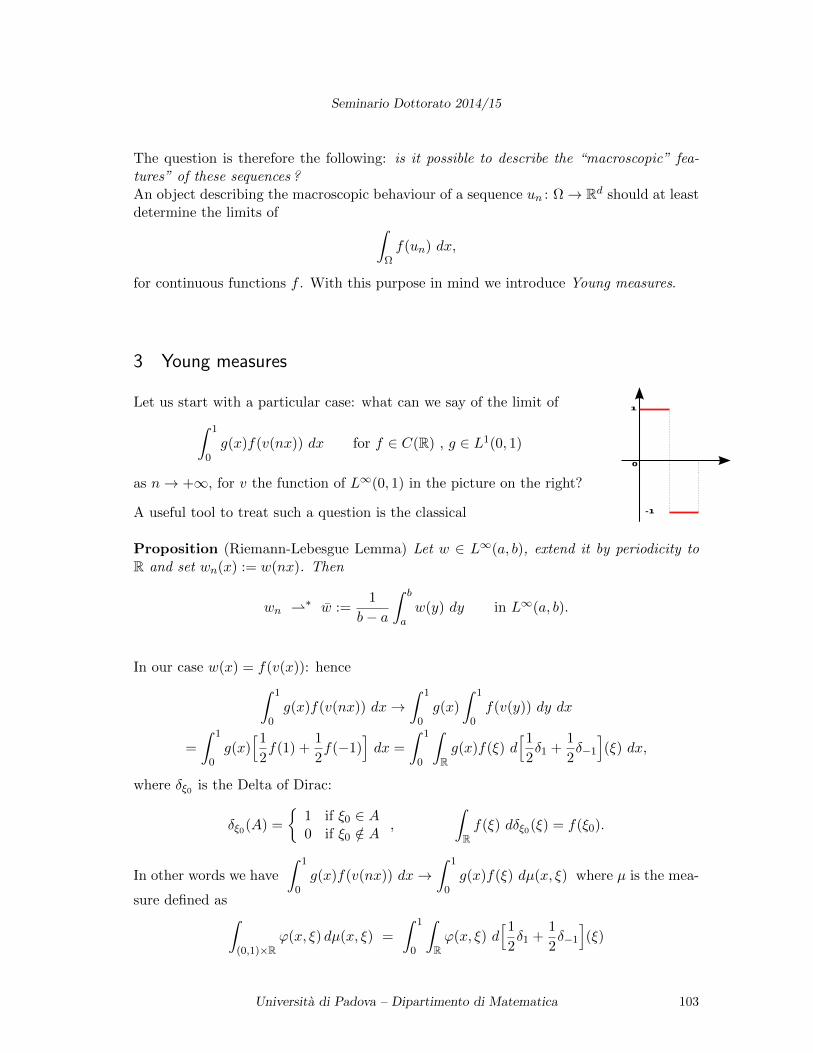
Seminario Dottorato 2014/15
The question is therefore the following: is it possible to describe the “macroscopic” fea-tures” of these sequences ?An object describing the macroscopic behaviour of a sequence un : Ω→ Rd should at leastdetermine the limits of ∫
Ωf(un) dx,
for continuous functions f . With this purpose in mind we introduce Young measures.
3 Young measures
Let us start with a particular case: what can we say of the limit of∫ 1
0g(x)f(v(nx)) dx for f ∈ C(R) , g ∈ L1(0, 1)
as n→ +∞, for v the function of L∞(0, 1) in the picture on the right?
A useful tool to treat such a question is the classical
1
0
-1
0
-1
1
1
-1
0
1
0
-1
Proposition (Riemann-Lebesgue Lemma) Let w ∈ L∞(a, b), extend it by periodicity toR and set wn(x) := w(nx). Then
wn ∗ w :=1
b− a
∫ b
aw(y) dy in L∞(a, b).
In our case w(x) = f(v(x)): hence∫ 1
0g(x)f(v(nx)) dx→
∫ 1
0g(x)
∫ 1
0f(v(y)) dy dx
=
∫ 1
0g(x)
[1
2f(1) +
1
2f(−1)
]dx =
∫ 1
0
∫Rg(x)f(ξ) d
[1
2δ1 +
1
2δ−1
](ξ) dx,
where δξ0 is the Delta of Dirac:
δξ0(A) =
1 if ξ0 ∈ A0 if ξ0 /∈ A
,
∫Rf(ξ) dδξ0(ξ) = f(ξ0).
In other words we have
∫ 1
0g(x)f(v(nx)) dx→
∫ 1
0g(x)f(ξ) dµ(x, ξ) where µ is the mea-
sure defined as∫(0,1)×R
ϕ(x, ξ) dµ(x, ξ) =
∫ 1
0
∫Rϕ(x, ξ) d
[1
2δ1 +
1
2δ−1
](ξ)
Universita di Padova – Dipartimento di Matematica 103
Seminario Dottorato 2014/15
for every bounded Borel function ϕ. We say that µ is the Young measure associated withthe minimizing sequence vn. In general, a Young measure µ on Ω with values in Rd canbe identified with a measurable family (µx)x∈Ω of probability measures µx on Rd by∫
Ω×Rϕ(x, ξ) dµ(x, ξ) =
∫Ω
∫Rϕ(x, ξ) dµx(ξ) dx
for every bounded Borel function ϕ.
Coming back to our modeling problem, we need to translate it in terms of Young measuresas summarized in the following table, where the question marks represent the still uncleartranslations:
Functions Young measures
v : Ω→ Rd (δv(x))x∈Ω measure on Ω× Rd∫ΩW (x, v(x)) dx
∫Ω×Rd
W (x, ξ) dδv(x)(ξ)dx
‖vn‖p bounded (p > 1) ?⇒ vn v weakly in Lp
(up to a subsequence)
∫ΩW (x, vn(x)) dx
∫Ω×RN W (x, ξ) dδvn(x)(ξ)dx
not lower semicontinuous with ?respect to weak convergence in Lp
To clear these question marks out, we must define a suitable topology on the spaceY (Ω;Rd) of Young measures and clarify some related notions: let us give a brief sketch ofthat.
Let C0(Ω × Rd) be the space of continuous functions ϕ such that the sets |ϕ| ≥ ε arecompact for any ε > 0, and let Mb(Ω×Rd) be the space of bounded Radon measures, i.e.the dual space of C0(Ω×Rd): therefore, for µ ∈Mb(Ω×Rd) and ϕ ∈ C0(Ω×Rd) we havea duality represented by 〈ϕ, µ〉 =
∫Ω×Rd ϕ dµ. From this duality we inherit a notion of
weak* convergence, as follows:
µn ∗ µ ⇐⇒
∫ϕ dµn →
∫ϕ dµ for any ϕ ∈ C0(Ω× Rd).
A Young measure µ = (µx)x∈Ω is an element of M+b (Ω×Rd) satisfying µ(A× Rd) = LN (A)
for every measurable set A ⊂ Ω: hence in particular Y (Ω;Rd) inherits the weak* topology
Universita di Padova – Dipartimento di Matematica 104
Seminario Dottorato 2014/15
from Mb(Ω × Rd). Moreover, if ϕ is continuous and ϕ ≥ 0, then the function µn 7→∫Ω×Rd ϕ(x, ξ) dµn is lower semicontinuous with respect to weak* convergence.
The p-moments of a Young measure µ are defined as∫
Ω×Rd |ξ|p dµ . If the p-moments of
a sequence (µn)n are equibounded we can deduce that (µn)n converges weakly*, up to asubsequence.Now, the p-moments of a sequence of Young measures µn associated with functions (∇un)n(i.e. µn = (δ∇un(x))x∈Ω) are ‖∇un‖Lp . Since the growth condition W (x, F ) ≥ a|F |p + b(x)implies ‖∇un‖Lp < C for any n, if un is a minimizing sequence we deduce that the p-moments of minimizing sequences are equibounded.Hence, thanks to the compactness property and the lower semicontinuity property de-scribed here before, using the Direct Method we can find a minimizer in Y (Ω;Rd).
We can then complete the table above:
Functions Young measures
v : Ω→ Rd (δv(x))x∈Ω measure on Ω× Rd∫ΩW (x, v(x)) dx
∫Ω×Rd
W (x, ξ) dδv(x)(ξ)dx
‖vn‖p bounded (p > 1) (δvn(x))x with equibounded p-moments
⇒ vn v weakly in Lp ⇒ (δvn(x))x µ weakly*
(up to a subsequence) (up to a subsequence)
∫ΩW (x, vn(x)) dx
∫Ω×RN W (x, ξ) dδvn(x)(ξ)dx
not lower semicontinuous with lower semicontinuous withrespect to weak convergence in Lp respect to weak* convergence
4 An example: Young measures and microstructures
A microstructure is any structure on a scale between macroscopic scale and the atomicscale. In a variational model, microstructures are formed to try to satisfy an optimalityproperty.
Example Solid-solid phase transitions in certain elastic crystals (the picture shows a microstruc-ture in Cu-Al-Ni).
Universita di Padova – Dipartimento di Matematica 105
Seminario Dottorato 2014/15
– Above the critical temperature θ0, Wθ(A) = 0
– Below the critical temperature, change of stability of the crystal structure:Wθ(B) = 0
– At the critical temperature both phases are stable: Wθ0(A) = Wθ0(B) = 0
Boundary conditions are typically caused by contacts with other part of the crystal where otherdeformation gradients prevail.
A nontrivial boundary condition λA+(1−λ)B causes no exact solutions: finer and finer mixturesof A and B are requested, and this is ilustrated by an equilibrium configuration given in terms ofYoung measures.
References
[1] B. Dacorogna, “Introduction to the Calculus of Variations”. Third Edition. Imperial CollegePress, London, 2015.
[2] S. Muller, Variational Models for microstructure and phase transitions. Calculus of Variationsand geometric evolution problems (Cetraro, 1996). Lecture Notes in Math., 1713, Springer,Berlin, 1999.
[3] P. Pedregal, “Parametrized Measures and Variational Principles”. Birkhauser-Verlag, Basel,Switzerland, 1997.
[4] P. Pedregal, “Variational Methods in Nonlinear Elasticity”. Society for Industrial and AppliedMathematics (SIAM), Philadelphia, 2000.
Universita di Padova – Dipartimento di Matematica 106
Seminario Dottorato 2014/15
Controllability and the numerical
approximation of the minimum time function
Thuy T.T. Le (∗)
Abstract. In optimal control theory, minimum time problems are of interest since they appearin many applications such as robotics, automotive, car industry, etc.. The scope of this talk isto give a brief introduction of these problems. Controllability conditions under various settingsare considered. Such conditions play a vital role in studying the regularity of the minimum timefunction T (x). Moreover, we will also introduce the HJB equation associated with a minimumtime problem and approaches to computing T (x) approximately.
1 Preliminary
1.1 Control theory
A standard reference is [1]. Consider the following controlled dynamics in Rn
(1.1)
y(t) = f(y(t), u(t)), t ∈ [0,+∞) a.e.
y(0) = ξ ∈ Rn,
where
+ U ∈ Rm is a control set
+ u : [0,+∞)→ U is a control function
Let S ∈ Rn be a target set and the set of admissible controls is defined as
Uad = u : [0,+∞)→ U : u is measurable.
The following assumptions are supposed to be satisfied in the sequel.
(∗)Ph.D. course, Universita di Padova, Dip. Matematica, via Trieste 63, I-35121 Padova, Italy; E-mail:. Seminar held on May 27th, 20145.
Universita di Padova – Dipartimento di Matematica 107
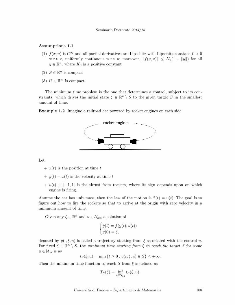
Seminario Dottorato 2014/15
Assumptions 1.1
(1) f(x, u) is C∞ and all partial derivatives are Lipschitz with Lipschitz constant L > 0w.r.t x, uniformly continuous w.r.t u; moreover, ‖f(y, u)‖ ≤ K0(1 + ‖y‖) for ally ∈ Rn, where K0 is a positive constant
(2) S ∈ Rn is compact
(3) U ∈ Rm is compact
The minimum time problem is the one that determines a control, subject to its con-straints, which drives the initial state ξ ∈ Rn \ S to the given target S in the smallestamount of time.
Example 1.2 Imagine a railroad car powered by rocket engines on each side.
Let
+ x(t) is the position at time t
+ y(t) = x(t) is the velocity at time t
+ u(t) ∈ [−1, 1] is the thrust from rockets, where its sign depends upon on whichengine is firing.
Assume the car has unit mass, then the law of the motion is x(t) = u(t). The goal is tofigure out how to fire the rockets so that to arrive at the origin with zero velocity in aminimum amount of time.
Given any ξ ∈ Rn and u ∈ Uad, a solution ofy(t) = f(y(t), u(t))
y(0) = ξ,
denoted by y(·, ξ, u) is called a trajectory starting from ξ associated with the control u.For fixed ξ ∈ Rn \ S, the minimum time starting from ξ to reach the target S for someu ∈ Uad is as
tS(ξ, u) = min t ≥ 0 : y(t, ξ, u) ∈ S ≤ +∞.
Then the minimum time function to reach S from ξ is defined as
TS(ξ) = infu∈Uad
tS(ξ, u).
Universita di Padova – Dipartimento di Matematica 108
Seminario Dottorato 2014/15
We also define the reachable sets for time t ≥ 0 as follows.
RS(t) = ξ ∈ Rn : TS(ξ) < t
is the set of starting points from which the system can reach the target in time less thant.
RS = ξ ∈ Rn : TS(ξ) < +∞
is the set of starting points from which the system can reach the target in finite time.
1.2 Nonsmooth analysis
Now we will introduce some basic notions in nonsmooth analysis which are needed in thiscontext, see [3].
Definition 1.3 Let S ∈ Rn be closed and ρ > 0 be given. S satisfies a ρ–internal spherecondition if for any x ∈ S there exists y such that x ∈ B(y, ρ) ⊂ S.
Definition 1.4 Let Ω ⊂ Rn be an open set. A function g : Ω→ R is locally semiconcaveif for every x ∈ Ω there exists a ball B(x, r) and a positive constant C such that
(1.2) λg(y) + (1− λ)g(y′) ≤ g(λy + (1− λ)y′) + C∥∥y − y′∥∥2
for all y, y′ ∈ B(x, r) and all λ ∈ [0, 1].
Global semiconcavity means that the above inequality is satisfied by every y, y′ ∈ Ωsuch that the segment [y, y′] ⊂ Ω with the same constant C. The constant C appearingin (1.2) is labeled as semiconcavity constant.
Example 1.5 The distance function to B(0, r), dB(0,r)
(x) = |x| − r, is semiconcave with
semiconcavity 1r .
Definition 1.6 Let Ω ⊂ Rn be an open set, g : Ω → R. We say that a vector p belongsto the proximal superdifferential of g at x (notated by p ∈ ∂P g(x)) if there exist σ > 0such that
g(y) ≤ g(x) + 〈p, y − x〉+ σ ‖y − x‖2
for all y in a neighborhood of x.
2 Controllability
This section is devoted to small–time controllability of a given system and sufficient con-ditions to guarantee that property.
Definition 2.1 The system (f, U) is
Universita di Padova – Dipartimento di Matematica 109
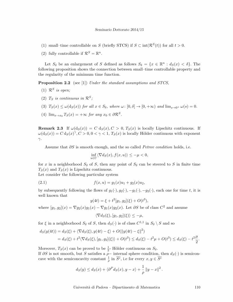
Seminario Dottorato 2014/15
(1) small–time controllable on S (briefly STCS) if S ⊂ int(RS(t)) for all t > 0.
(2) fully controllable if RS = Rn.
Let Sδ be an enlargement of S defined as follows Sδ = x ∈ Rn : dS(x) < δ. Thefollowing proposition shows the connection between small–time controllable property andthe regularity of the minimum time function.
Proposition 2.2 (see [1]) Under the standard assumptions and STCS,
(1) RS is open;
(2) TS is continuous in RS;
(3) TS(x) ≤ ω(dS(x)) for all x ∈ Sδ, where ω : [0, δ]→ [0,+∞) and lims→0+ ω(s) = 0.
(4) limx→x0 TS(x) = +∞ for any x0 ∈ ∂RS.
Remark 2.3 If ω(dS(x)) = C dS(x), C > 0, TS(x) is locally Lipschitz continuous. Ifω(dS(x)) = C dS(x)γ , C > 0, 0 < γ < 1, TS(x) is locally Holder continuous with exponentγ.
Assume that ∂S is smooth enough, and the so called Petrov condition holds, i.e.
infu∈U〈∇dS(x), f(x, u)〉 ≤ −µ < 0,
for x in a neighborhood Sδ of S, then any point of Sδ can be steered to S in finite timeTS(x) and TS(x) is Lipschitz continuous.Let consider the following particular system
(2.1) f(x, u) = g1(x)u1 + g2(x)u2,
by subsequently following the flows of g1(·), g2(·),−g1(·),−g2(·), each one for time t, it iswell known that
y(4t) = ξ + t2[g1, g2](ξ) +O(t3),
where [g1, g2](x) = ∇g2(x)g1(x)−∇g1(x)g2(x). Let ∂S be of class C2 and assume
〈∇dS(ξ), [g1, g2](ξ)〉 ≤ −µ,
for ξ in a neighborhood Sδ of S, then dS(·) is of class C1,1 in Sδ \ S and so
dS(y(4t)) = dS(ξ) + 〈∇dS(ξ), y(4t)− ξ〉+O(‖y(4t)− ξ‖2)
= dS(ξ) + t2〈∇dS(ξ), [g1, g2](ξ)〉+O(t3) ≤ dS(ξ)− t2µ+O(t3) ≤ dS(ξ)− t2µ2.
Moreover, TS(x) can be proved to be 12 - Holder continuous on Sδ.
If ∂S is not smooth, but S satisfies a ρ− internal sphere condition, then dS(·) is semicon-cave with the semiconcavity constant 1
ρ in Sc, i.e for every x, y ∈ Sc
dS(y) ≤ dS(x) + 〈∂PdS(x), y − x〉+1
ρ‖y − x‖2 .
Universita di Padova – Dipartimento di Matematica 110
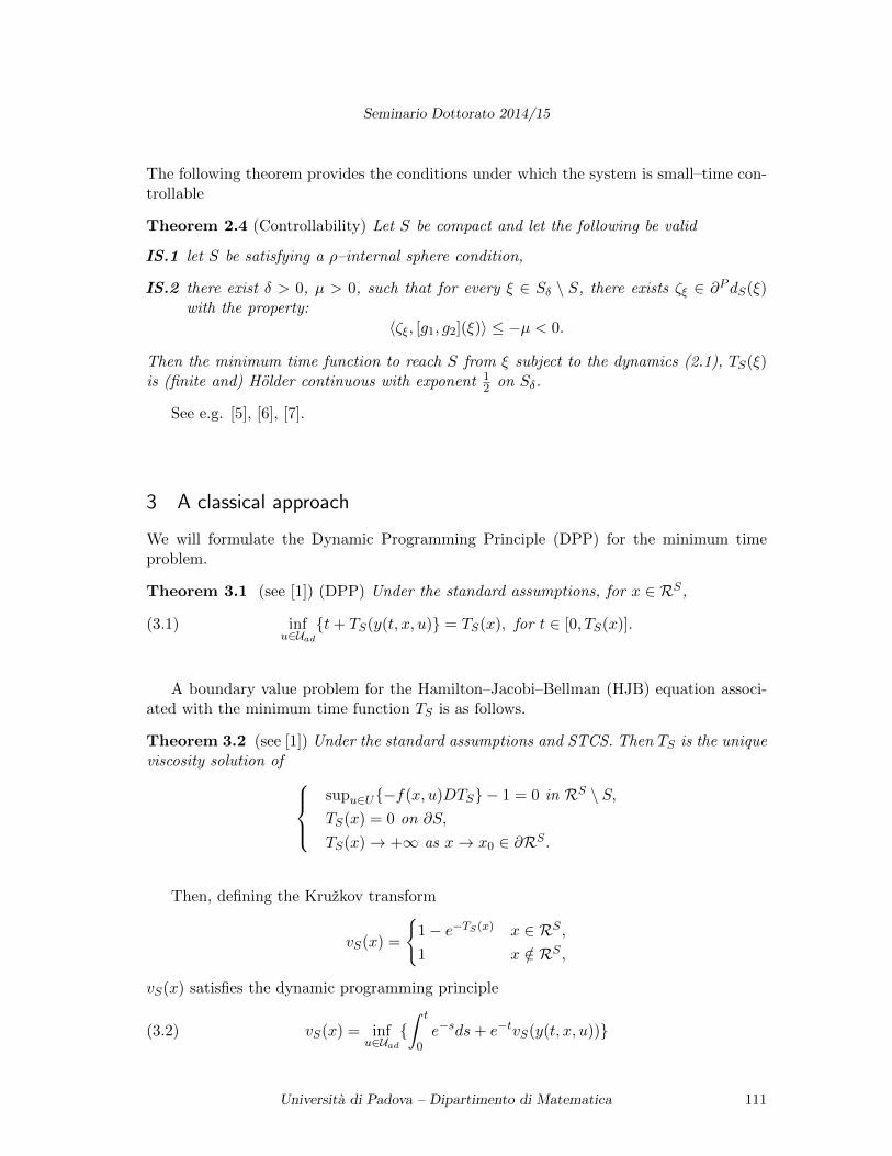
Seminario Dottorato 2014/15
The following theorem provides the conditions under which the system is small–time con-trollable
Theorem 2.4 (Controllability) Let S be compact and let the following be valid
IS.1 let S be satisfying a ρ–internal sphere condition,
IS.2 there exist δ > 0, µ > 0, such that for every ξ ∈ Sδ \ S, there exists ζξ ∈ ∂PdS(ξ)with the property:
〈ζξ, [g1, g2](ξ)〉 ≤ −µ < 0.
Then the minimum time function to reach S from ξ subject to the dynamics (2.1), TS(ξ)is (finite and) Holder continuous with exponent 1
2 on Sδ.
See e.g. [5], [6], [7].
3 A classical approach
We will formulate the Dynamic Programming Principle (DPP) for the minimum timeproblem.
Theorem 3.1 (see [1]) (DPP) Under the standard assumptions, for x ∈ RS,
(3.1) infu∈Uad
t+ TS(y(t, x, u) = TS(x), for t ∈ [0, TS(x)].
A boundary value problem for the Hamilton–Jacobi–Bellman (HJB) equation associ-ated with the minimum time function TS is as follows.
Theorem 3.2 (see [1]) Under the standard assumptions and STCS. Then TS is the uniqueviscosity solution of
supu∈U−f(x, u)DTS − 1 = 0 in RS \ S,TS(x) = 0 on ∂S,
TS(x)→ +∞ as x→ x0 ∈ ∂RS .
Then, defining the Kruzkov transform
vS(x) =
1− e−TS(x) x ∈ RS ,1 x /∈ RS ,
vS(x) satisfies the dynamic programming principle
(3.2) vS(x) = infu∈Uad
∫ t
0e−sds+ e−tvS(y(t, x, u))
Universita di Padova – Dipartimento di Matematica 111
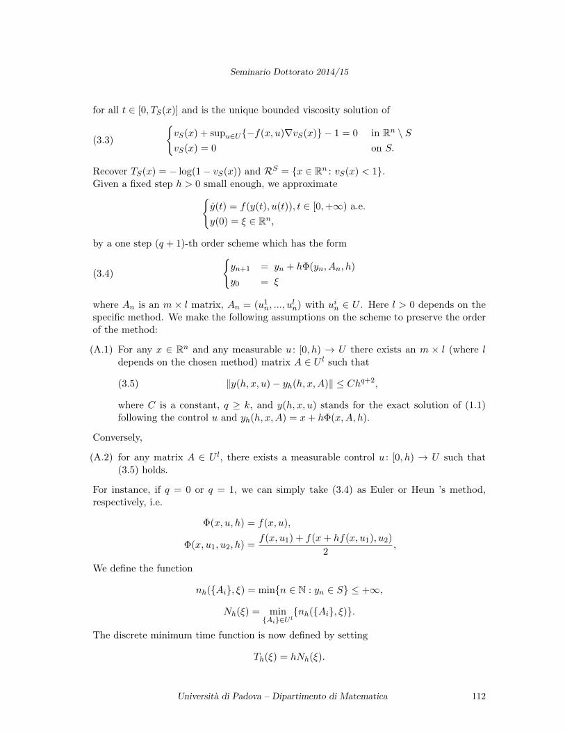
Seminario Dottorato 2014/15
for all t ∈ [0, TS(x)] and is the unique bounded viscosity solution of
(3.3)
vS(x) + supu∈U−f(x, u)∇vS(x) − 1 = 0 in Rn \ SvS(x) = 0 on S.
Recover TS(x) = − log(1− vS(x)) and RS = x ∈ Rn : vS(x) < 1.Given a fixed step h > 0 small enough, we approximate
y(t) = f(y(t), u(t)), t ∈ [0,+∞) a.e.
y(0) = ξ ∈ Rn,
by a one step (q + 1)-th order scheme which has the form
(3.4)
yn+1 = yn + hΦ(yn, An, h)
y0 = ξ
where An is an m × l matrix, An = (u1n, ..., u
ln) with uin ∈ U . Here l > 0 depends on the
specific method. We make the following assumptions on the scheme to preserve the orderof the method:
(A.1) For any x ∈ Rn and any measurable u : [0, h) → U there exists an m × l (where ldepends on the chosen method) matrix A ∈ U l such that
(3.5) ‖y(h, x, u)− yh(h, x,A)‖ ≤ Chq+2,
where C is a constant, q ≥ k, and y(h, x, u) stands for the exact solution of (1.1)following the control u and yh(h, x,A) = x+ hΦ(x,A, h).
Conversely,
(A.2) for any matrix A ∈ U l, there exists a measurable control u : [0, h) → U such that(3.5) holds.
For instance, if q = 0 or q = 1, we can simply take (3.4) as Euler or Heun ’s method,respectively, i.e.
Φ(x, u, h) = f(x, u),
Φ(x, u1, u2, h) =f(x, u1) + f(x+ hf(x, u1), u2)
2,
We define the function
nh(Ai, ξ) = minn ∈ N : yn ∈ S ≤ +∞,
Nh(ξ) = minAi∈U l
nh(Ai, ξ).
The discrete minimum time function is now defined by setting
Th(ξ) = hNh(ξ).
Universita di Padova – Dipartimento di Matematica 112
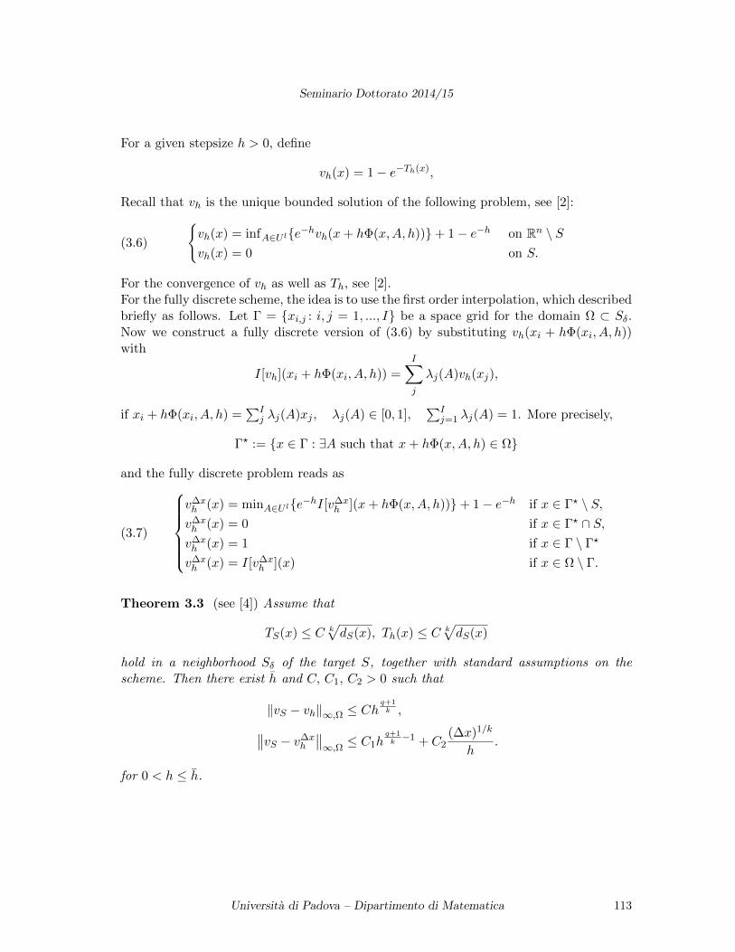
Seminario Dottorato 2014/15
For a given stepsize h > 0, define
vh(x) = 1− e−Th(x),
Recall that vh is the unique bounded solution of the following problem, see [2]:
(3.6)
vh(x) = infA∈U le−hvh(x+ hΦ(x,A, h))+ 1− e−h on Rn \ Svh(x) = 0 on S.
For the convergence of vh as well as Th, see [2].For the fully discrete scheme, the idea is to use the first order interpolation, which describedbriefly as follows. Let Γ = xi,j : i, j = 1, ..., I be a space grid for the domain Ω ⊂ Sδ.Now we construct a fully discrete version of (3.6) by substituting vh(xi + hΦ(xi, A, h))with
I[vh](xi + hΦ(xi, A, h)) =
I∑j
λj(A)vh(xj),
if xi + hΦ(xi, A, h) =∑I
j λj(A)xj , λj(A) ∈ [0, 1],∑I
j=1 λj(A) = 1. More precisely,
Γ? := x ∈ Γ : ∃A such that x+ hΦ(x,A, h) ∈ Ω
and the fully discrete problem reads as
(3.7)
v∆xh (x) = minA∈U le−hI[v∆x
h ](x+ hΦ(x,A, h))+ 1− e−h if x ∈ Γ? \ S,v∆xh (x) = 0 if x ∈ Γ? ∩ S,v∆xh (x) = 1 if x ∈ Γ \ Γ?
v∆xh (x) = I[v∆x
h ](x) if x ∈ Ω \ Γ.
Theorem 3.3 (see [4]) Assume that
TS(x) ≤ C k√dS(x), Th(x) ≤ C k
√dS(x)
hold in a neighborhood Sδ of the target S, together with standard assumptions on thescheme. Then there exist h and C, C1, C2 > 0 such that
‖vS − vh‖∞,Ω ≤ Chq+1k ,∥∥vS − v∆x
h
∥∥∞,Ω ≤ C1h
q+1k−1 + C2
(∆x)1/k
h.
for 0 < h ≤ h.
Universita di Padova – Dipartimento di Matematica 113
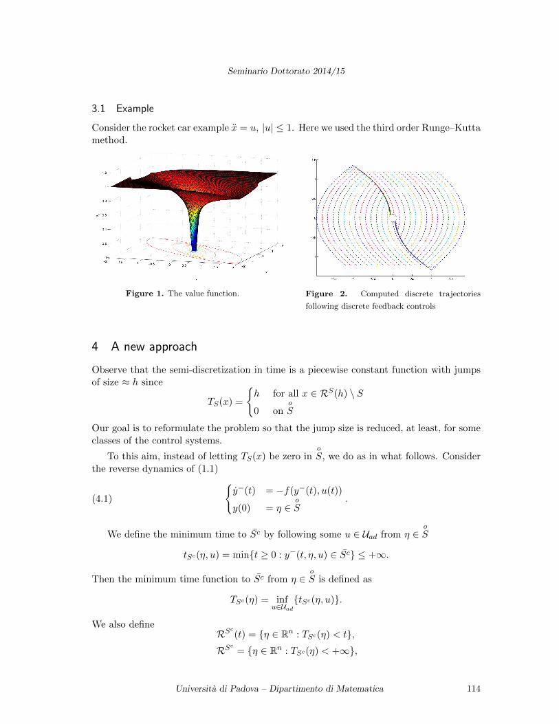
Seminario Dottorato 2014/15
3.1 Example
Consider the rocket car example x = u, |u| ≤ 1. Here we used the third order Runge–Kuttamethod.
Figure 1. The value function. Figure 2. Computed discrete trajectories
following discrete feedback controls
4 A new approach
Observe that the semi-discretization in time is a piecewise constant function with jumpsof size ≈ h since
TS(x) =
h for all x ∈ RS(h) \ S
0 onoS
Our goal is to reformulate the problem so that the jump size is reduced, at least, for someclasses of the control systems.
To this aim, instead of letting TS(x) be zero inoS, we do as in what follows. Consider
the reverse dynamics of (1.1)
(4.1)
y−(t) = −f(y−(t), u(t))
y(0) = η ∈oS
.
We define the minimum time to Sc by following some u ∈ Uad from η ∈oS
tSc(η, u) = mint ≥ 0 : y−(t, η, u) ∈ Sc ≤ +∞.
Then the minimum time function to Sc from η ∈oS is defined as
TSc(η) = infu∈Uad
tSc(η, u).
We also defineRSc(t) = η ∈ Rn : TSc(η) < t,RSc = η ∈ Rn : TSc(η) < +∞,
Universita di Padova – Dipartimento di Matematica 114
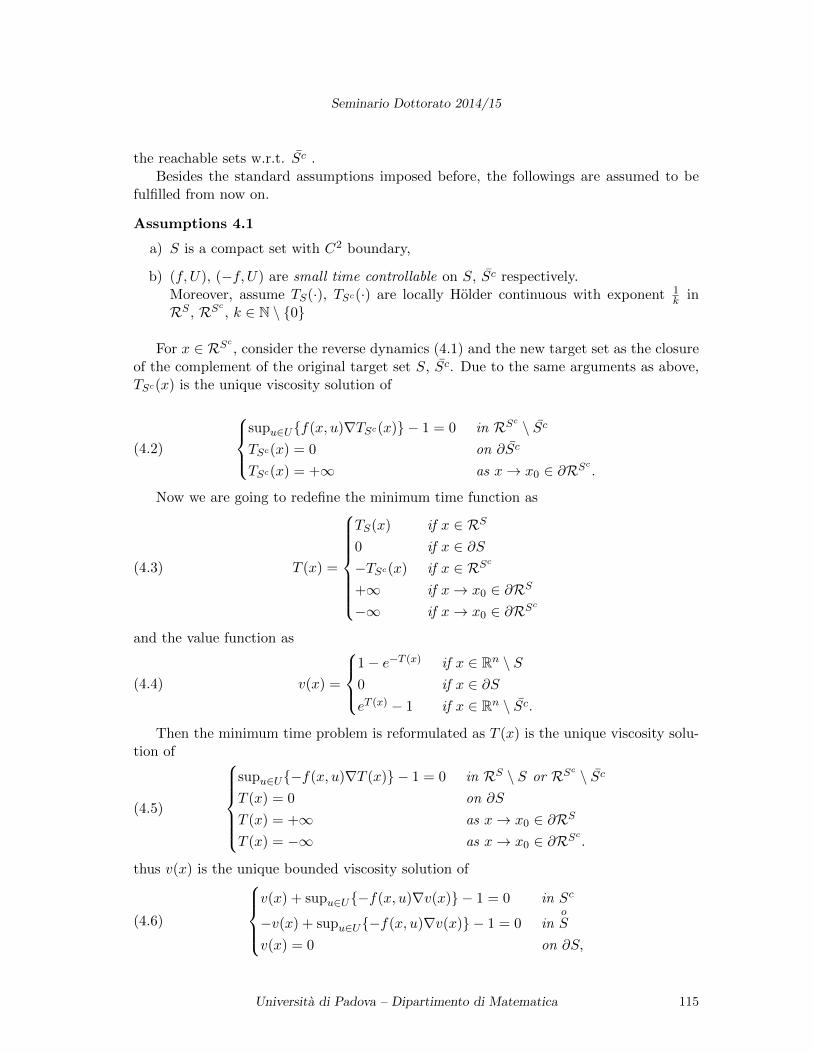
Seminario Dottorato 2014/15
the reachable sets w.r.t. Sc .Besides the standard assumptions imposed before, the followings are assumed to be
fulfilled from now on.
Assumptions 4.1
a) S is a compact set with C2 boundary,
b) (f, U), (−f, U) are small time controllable on S, Sc respectively.Moreover, assume TS(·), TSc(·) are locally Holder continuous with exponent 1
k inRS , RSc , k ∈ N \ 0
For x ∈ RSc , consider the reverse dynamics (4.1) and the new target set as the closureof the complement of the original target set S, Sc. Due to the same arguments as above,TSc(x) is the unique viscosity solution of
(4.2)
supu∈Uf(x, u)∇TSc(x) − 1 = 0 in RSc \ Sc
TSc(x) = 0 on ∂Sc
TSc(x) = +∞ as x→ x0 ∈ ∂RSc.
Now we are going to redefine the minimum time function as
(4.3) T (x) =
TS(x) if x ∈ RS
0 if x ∈ ∂S−TSc(x) if x ∈ RSc
+∞ if x→ x0 ∈ ∂RS
−∞ if x→ x0 ∈ ∂RSc
and the value function as
(4.4) v(x) =
1− e−T (x) if x ∈ Rn \ S0 if x ∈ ∂SeT (x) − 1 if x ∈ Rn \ Sc.
Then the minimum time problem is reformulated as T (x) is the unique viscosity solu-tion of
(4.5)
supu∈U−f(x, u)∇T (x) − 1 = 0 in RS \ S or RSc \ Sc
T (x) = 0 on ∂S
T (x) = +∞ as x→ x0 ∈ ∂RS
T (x) = −∞ as x→ x0 ∈ ∂RSc.
thus v(x) is the unique bounded viscosity solution of
(4.6)
v(x) + supu∈U−f(x, u)∇v(x) − 1 = 0 in Sc
−v(x) + supu∈U−f(x, u)∇v(x) − 1 = 0 inoS
v(x) = 0 on ∂S,
Universita di Padova – Dipartimento di Matematica 115
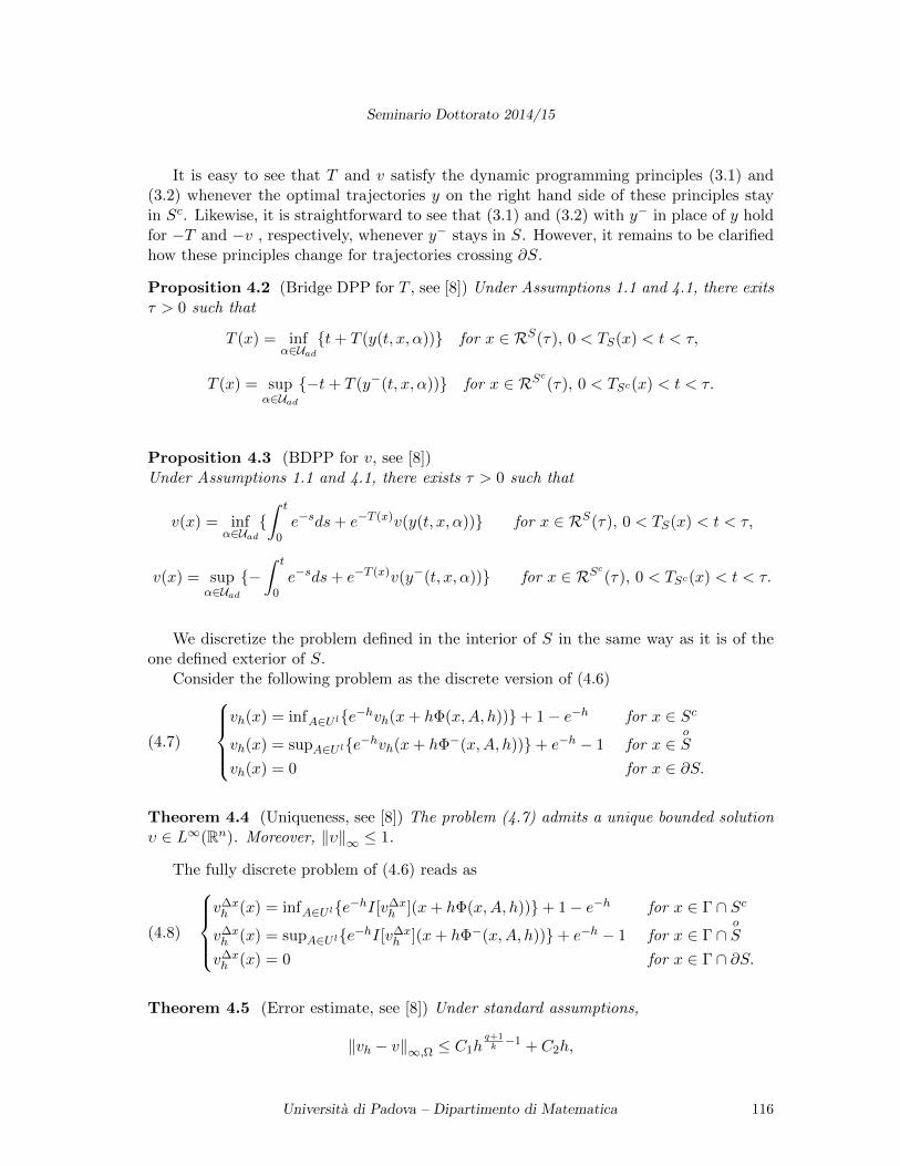
Seminario Dottorato 2014/15
It is easy to see that T and v satisfy the dynamic programming principles (3.1) and(3.2) whenever the optimal trajectories y on the right hand side of these principles stayin Sc. Likewise, it is straightforward to see that (3.1) and (3.2) with y− in place of y holdfor −T and −v , respectively, whenever y− stays in S. However, it remains to be clarifiedhow these principles change for trajectories crossing ∂S.
Proposition 4.2 (Bridge DPP for T , see [8]) Under Assumptions 1.1 and 4.1, there exitsτ > 0 such that
T (x) = infα∈Uad
t+ T (y(t, x, α)) for x ∈ RS(τ), 0 < TS(x) < t < τ,
T (x) = supα∈Uad
−t+ T (y−(t, x, α)) for x ∈ RSc(τ), 0 < TSc(x) < t < τ.
Proposition 4.3 (BDPP for v, see [8])Under Assumptions 1.1 and 4.1, there exists τ > 0 such that
v(x) = infα∈Uad
∫ t
0e−sds+ e−T (x)v(y(t, x, α)) for x ∈ RS(τ), 0 < TS(x) < t < τ,
v(x) = supα∈Uad
−∫ t
0e−sds+ e−T (x)v(y−(t, x, α)) for x ∈ RSc(τ), 0 < TSc(x) < t < τ.
We discretize the problem defined in the interior of S in the same way as it is of theone defined exterior of S.
Consider the following problem as the discrete version of (4.6)
(4.7)
vh(x) = infA∈U le−hvh(x+ hΦ(x,A, h))+ 1− e−h for x ∈ Sc
vh(x) = supA∈U le−hvh(x+ hΦ−(x,A, h))+ e−h − 1 for x ∈oS
vh(x) = 0 for x ∈ ∂S.
Theorem 4.4 (Uniqueness, see [8]) The problem (4.7) admits a unique bounded solutionυ ∈ L∞(Rn). Moreover, ‖υ‖∞ ≤ 1.
The fully discrete problem of (4.6) reads as
(4.8)
v∆xh (x) = infA∈U le−hI[v∆x
h ](x+ hΦ(x,A, h))+ 1− e−h for x ∈ Γ ∩ Sc
v∆xh (x) = supA∈U le−hI[v∆x
h ](x+ hΦ−(x,A, h))+ e−h − 1 for x ∈ Γ ∩oS
v∆xh (x) = 0 for x ∈ Γ ∩ ∂S.
Theorem 4.5 (Error estimate, see [8]) Under standard assumptions,
‖vh − v‖∞,Ω ≤ C1hq+1k−1 + C2h,
Universita di Padova – Dipartimento di Matematica 116
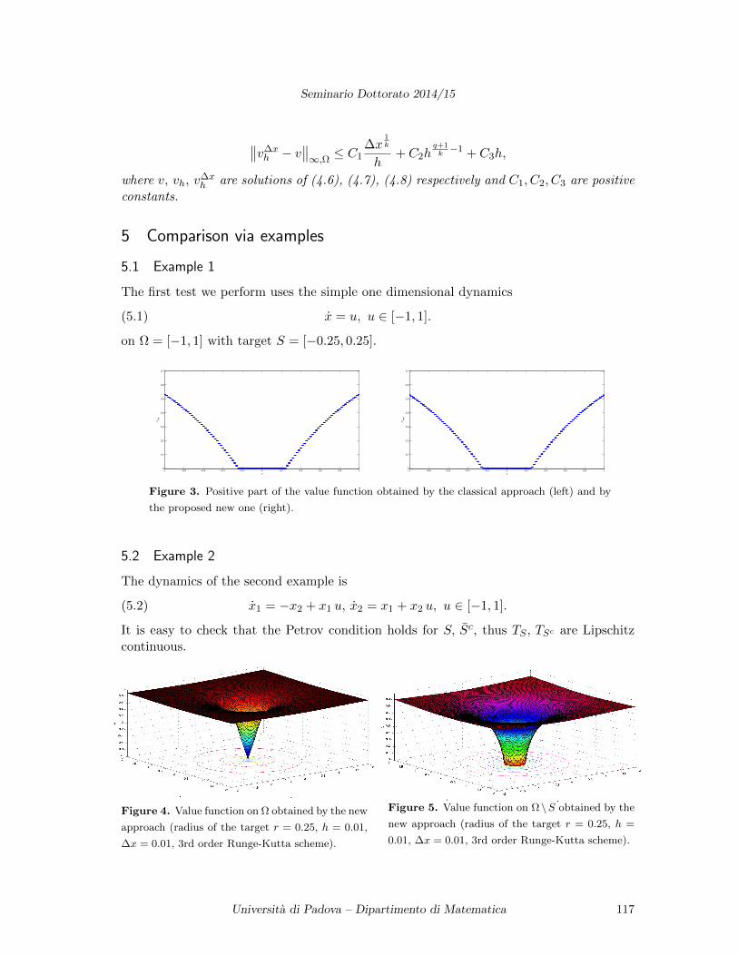
Seminario Dottorato 2014/15
∥∥v∆xh − v
∥∥∞,Ω ≤ C1
∆x1k
h+ C2h
q+1k−1 + C3h,
where v, vh, v∆xh are solutions of (4.6), (4.7), (4.8) respectively and C1, C2, C3 are positive
constants.
5 Comparison via examples
5.1 Example 1
The first test we perform uses the simple one dimensional dynamics
(5.1) x = u, u ∈ [−1, 1].
on Ω = [−1, 1] with target S = [−0.25, 0.25].
−1 −0.8 −0.6 −0.4 −0.2 0 0.2 0.4 0.6 0.8 10
0.1
0.2
0.3
0.4
0.5
0.6
0.7
x
Vol
d
−1 −0.8 −0.6 −0.4 −0.2 0 0.2 0.4 0.6 0.8 10
0.1
0.2
0.3
0.4
0.5
0.6
0.7
x
Vne
w
Figure 3. Positive part of the value function obtained by the classical approach (left) and by
the proposed new one (right).
5.2 Example 2
The dynamics of the second example is
(5.2) x1 = −x2 + x1 u, x2 = x1 + x2 u, u ∈ [−1, 1].
It is easy to check that the Petrov condition holds for S, Sc, thus TS , TSc are Lipschitzcontinuous.
Figure 4. Value function on Ω obtained by the new
approach (radius of the target r = 0.25, h = 0.01,
∆x = 0.01, 3rd order Runge-Kutta scheme).
Figure 5. Value function on Ω\S obtained by the
new approach (radius of the target r = 0.25, h =
0.01, ∆x = 0.01, 3rd order Runge-Kutta scheme).
Universita di Padova – Dipartimento di Matematica 117
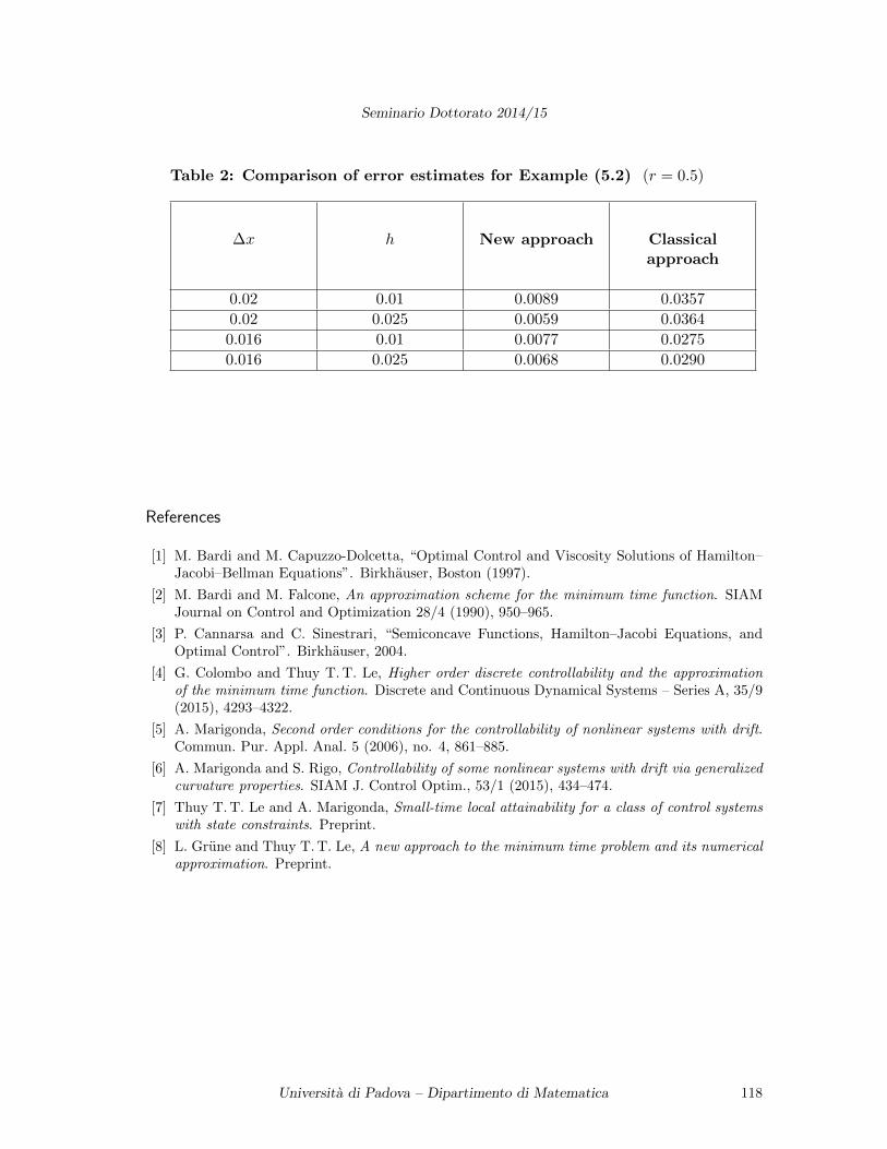
Seminario Dottorato 2014/15
Table 2: Comparison of error estimates for Example (5.2) (r = 0.5)
∆x h New approach Classicalapproach
0.02 0.01 0.0089 0.0357
0.02 0.025 0.0059 0.0364
0.016 0.01 0.0077 0.0275
0.016 0.025 0.0068 0.0290
References
[1] M. Bardi and M. Capuzzo-Dolcetta, “Optimal Control and Viscosity Solutions of Hamilton–Jacobi–Bellman Equations”. Birkhauser, Boston (1997).
[2] M. Bardi and M. Falcone, An approximation scheme for the minimum time function. SIAMJournal on Control and Optimization 28/4 (1990), 950–965.
[3] P. Cannarsa and C. Sinestrari, “Semiconcave Functions, Hamilton–Jacobi Equations, andOptimal Control”. Birkhauser, 2004.
[4] G. Colombo and Thuy T. T. Le, Higher order discrete controllability and the approximationof the minimum time function. Discrete and Continuous Dynamical Systems – Series A, 35/9(2015), 4293–4322.
[5] A. Marigonda, Second order conditions for the controllability of nonlinear systems with drift.Commun. Pur. Appl. Anal. 5 (2006), no. 4, 861–885.
[6] A. Marigonda and S. Rigo, Controllability of some nonlinear systems with drift via generalizedcurvature properties. SIAM J. Control Optim., 53/1 (2015), 434–474.
[7] Thuy T. T. Le and A. Marigonda, Small-time local attainability for a class of control systemswith state constraints. Preprint.
[8] L. Grune and Thuy T. T. Le, A new approach to the minimum time problem and its numericalapproximation. Preprint.
Universita di Padova – Dipartimento di Matematica 118
Seminario Dottorato 2014/15
An introduction to derived categories
Francesco Mattiello (∗)
Abstract. Derived categories were introduced in the sixties by Grothendieck and Verdier and haveproved to be of fundamental importance in Mathematics. Starting with a short review of the basiclanguage of category theory, we will first introduce the notion of abelian category with the help ofseveral examples. Then we will spend some time giving a thorough motivation for the constructionof the derived category of an abelian category.
Contents
Introduction . . . . . . . . . . . . . . . . . . . . . . . . . . . . . . . . . . . . . . . . . . . . . . . . . . . . . . . . . . . . . . . . . . . 1191. The language of category theory . . . . . . . . . . . . . . . . . . . . . . . . . . . . . . . . . . . . . . . . . . . . . 120
1.1. Categories . . . . . . . . . . . . . . . . . . . . . . . . . . . . . . . . . . . . . . . . . . . . . . . . . . . . . . . . . . . . . . . 1201.2. Products and coproducts . . . . . . . . . . . . . . . . . . . . . . . . . . . . . . . . . . . . . . . . . . . . . . . . 1221.3. Functors . . . . . . . . . . . . . . . . . . . . . . . . . . . . . . . . . . . . . . . . . . . . . . . . . . . . . . . . . . . . . . . . . 1231.4. Natural transformations . . . . . . . . . . . . . . . . . . . . . . . . . . . . . . . . . . . . . . . . . . . . . . . . . 124
2. Abelian categories . . . . . . . . . . . . . . . . . . . . . . . . . . . . . . . . . . . . . . . . . . . . . . . . . . . . . . . . . . . 1252.1. Additive categories . . . . . . . . . . . . . . . . . . . . . . . . . . . . . . . . . . . . . . . . . . . . . . . . . . . . . . 1252.2. Abelian categories . . . . . . . . . . . . . . . . . . . . . . . . . . . . . . . . . . . . . . . . . . . . . . . . . . . . . . . 127
3. Derived categories . . . . . . . . . . . . . . . . . . . . . . . . . . . . . . . . . . . . . . . . . . . . . . . . . . . . . . . . . . . 1293.1. The category of cochain complexes and the homotopy category . . . . . . . . . . . 1293.2. The derived category . . . . . . . . . . . . . . . . . . . . . . . . . . . . . . . . . . . . . . . . . . . . . . . . . . . . 131
References . . . . . . . . . . . . . . . . . . . . . . . . . . . . . . . . . . . . . . . . . . . . . . . . . . . . . . . . . . . . . . . . . . . . . 133
Introduction
Derived categories were introduced in the sixties by Grothendieck and Verdier in the studyof derived functors and spectral sequences.
Given an abelian category C, its derived category D(C) is obtained from the categoryCh(C) of (cochain) complexes in two stages. First one constructs a quotient K(C) of Ch(C)by identifying chain homotopy equivalent morphisms between complexes. Such a quotient
(∗)Ph.D. course, Universita di Padova, Dip. Matematica, via Trieste 63, I-35121 Padova, Italy; E-mail:. Seminar held on June 10th, 2015.
Universita di Padova – Dipartimento di Matematica 119
Seminario Dottorato 2014/15
category K(C) is called the homotopy category of C. It is an additive category in whichthe homotopy equivalences are invertible, but this advantage comes at a cost: K(C) isnot abelian anymore. Consequently, one has to look for an effective substitute for shortexact sequences, that should still have the property that it induces long exact sequenceson cohomology. The concept of a triangulated category with its “distinguished triangles”provides a solution. It turns out that the homotopy category K(C) can be endowed withthe structure of a triangulated category. The second step consists in “localizing” K(C) byinverting quasi-isomorphisms using a calculus of fractions. The goal is the following: wewant morphisms in K(C) which induce isomorphisms on cohomology to be invertible in thecategory to be constructed. If we want a quasi-isomorphism to become an isomorphism,it has to have an inverse. Unfortunately, there is no candidate for an inverse around. Soto define a derived category, we have to use a more elaborate process called localizationof categories.This short note is organized as follows. In Section 1 we recall the basic language ofcategory theory; in Section 2, we introduce predictive, additive and abelian categories;finally, in Section 3 we give a sketch of the construction of the derived category of anabelian category.The reader is referred to [1], [2], [3], [4], [5], [6], [7], [8].
1 The language of category theory
1.1 Categories
We recall that a category C consists of a class Ob(C) of objects, a set of morphismsHomC(A, B) (often denoted by Hom(A, B)) for every ordered pair (A, B) of objects,and a composition Hom(A, B)×Hom(B, C)→ Hom(A, C), denoted by (f, g) 7→ g f , for
every ordered triple A, B, C of objects. We often write f : A → B or Af→ B instead of
f ∈ Hom(A, B). The following axioms must be satisfied:
(a) the Hom sets are pairwise disjoint, that is, each f ∈ Hom(A, B) has a unique domainA and a unique target B;
(b) for each object A, there is an identity morphism 1A ∈ Hom(A, A) such that f 1A = fand 1B f = f for all f : A→ B;
(c) composition is associative: given morphisms Af //B
g //Ch //D , then h (g f) =
(h g) f .
There is a bijection between objects A and their identity morphisms 1A. Thus, wemay regard a category as consisting only of morphisms. In almost all uses of categories,however, it is more natural to think of two sorts of entries: objects and morphisms.
If C is a category, its opposite category Cop is the category with Ob(Cop) = Ob(C),with morphisms HomCop(A, B) = HomC(B, A) (we may write morphisms in Cop as fop,where f is a morphism in C), and with composition the reverse of that in C; that is,
gop fop = (f g)op. We illustrate the composition in Cop: a diagram Cfop //B
gop //A in Cop
Universita di Padova – Dipartimento di Matematica 120
Seminario Dottorato 2014/15
corresponds to the diagram Ag //B
f //C in C. Any concept or statement about anarbitrary category admits a dual concept or statement (the process of reversing arrows).
A category S is a subcategory of a category C if: Ob(S) ⊆ Ob(C); HomS(A, B) ⊆HomC(A, B) for all A, B ∈ Ob(S); if f ∈ HomS(A, B) and g ∈ HomS(B, C), then thecomposite g f ∈ HomS(A, C) is equal to the composite g f ∈ HomC(A, C); if A ∈ Ob(S),then the identity 1A ∈ HomS(A, A) is equal to the identity 1A ∈ HomC(A, A).A subcategory S of C is a full subcategory if, for all A, B ∈ Ob(S), we have HomS(A, B) =HomC(A, B).
A morphism u : B → C in a category C is a monomorphism (or is monic) if u can becanceled from the left; that is, for all objects A and all morphisms f, g : A→ B, we havethat u f = u g implies f = g.
Af //g// B
u // C.
It is clear that u : B → C is monic if and only if , for all A, the map u∗ : Hom(A, B) →Hom(A, C), u∗(f) = u f , is an injection.A morphism v : B → C in a category C is an epimorphism (or is epic) if v can be canceledfrom the right; that is for all objects D and all morphisms h, k : C → D, we have thath v = k v implies h = k.
Bv // C
h //
k// D.
It is clear that v : B → C is epic if and only if , for all D, the map v∗ : Hom(C, D) →Hom(B, D), v∗(f) = f v, is an injection.A morphism in a category C is a bijection if it is monic and epic.We call a left inverse (respectively, a right inverse) of u ∈ Hom(A, B) a morphismv ∈ Hom(B, A) such that v u = 1A (respectively u v = 1B); v is called the inverse ofu if it is both a left inverse and a right inverse of u (in which case it is uniquely deter-mined). The morphism u is called an isomorphism if it has an inverse. If u has a leftinverse (respectively, a right inverse) it is monic (respectively epic). Thus an isomorphismis bijective (the converse being, in general, false).The composite of two monomorphisms (respectively, epimorphisms) is a monomorphism(respectively, epimorphisms), hence the composite of two bijections is a bijection; simi-larly the composite of two isomorphisms is an isomorphism. If the composite v u of twomorphisms u, v is a monomorphism (respectively, an epimorphism), then u (respectively,v) is as well.
If B is an object in a category C, consider all ordered pairs (A, f), where f : A → Bis a monomorphism. Call two such pairs (A, f) and (A′, f ′) equivalent if there exists anisomorphism g : A′ → A with f ′ = f g.
Af // B
A′
g
OO
f ′
>>
Universita di Padova – Dipartimento di Matematica 121
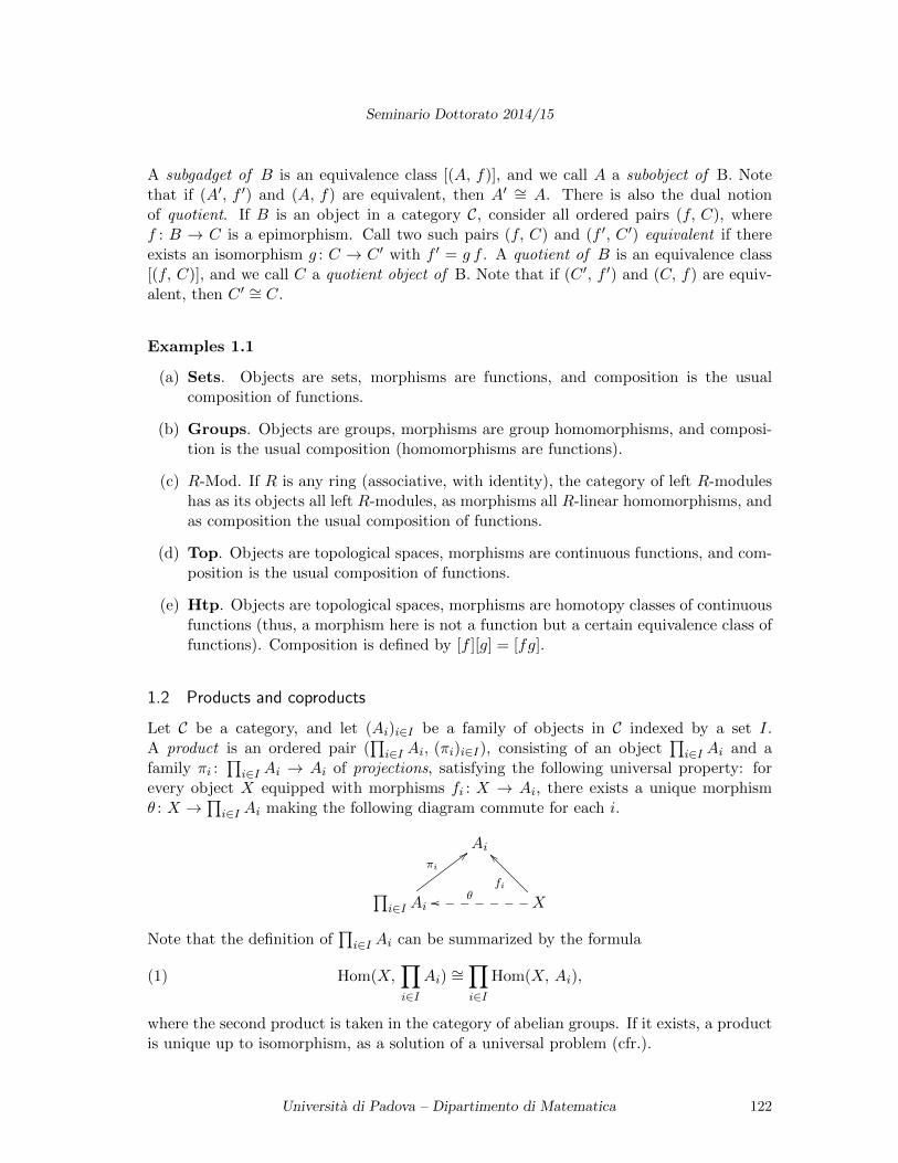
Seminario Dottorato 2014/15
A subgadget of B is an equivalence class [(A, f)], and we call A a subobject of B. Notethat if (A′, f ′) and (A, f) are equivalent, then A′ ∼= A. There is also the dual notionof quotient. If B is an object in a category C, consider all ordered pairs (f, C), wheref : B → C is a epimorphism. Call two such pairs (f, C) and (f ′, C ′) equivalent if thereexists an isomorphism g : C → C ′ with f ′ = g f . A quotient of B is an equivalence class[(f, C)], and we call C a quotient object of B. Note that if (C ′, f ′) and (C, f) are equiv-alent, then C ′ ∼= C.
Examples 1.1
(a) Sets. Objects are sets, morphisms are functions, and composition is the usualcomposition of functions.
(b) Groups. Objects are groups, morphisms are group homomorphisms, and composi-tion is the usual composition (homomorphisms are functions).
(c) R-Mod. If R is any ring (associative, with identity), the category of left R-moduleshas as its objects all left R-modules, as morphisms all R-linear homomorphisms, andas composition the usual composition of functions.
(d) Top. Objects are topological spaces, morphisms are continuous functions, and com-position is the usual composition of functions.
(e) Htp. Objects are topological spaces, morphisms are homotopy classes of continuousfunctions (thus, a morphism here is not a function but a certain equivalence class offunctions). Composition is defined by [f ][g] = [fg].
1.2 Products and coproducts
Let C be a category, and let (Ai)i∈I be a family of objects in C indexed by a set I.A product is an ordered pair (
∏i∈I Ai, (πi)i∈I), consisting of an object
∏i∈I Ai and a
family πi :∏i∈I Ai → Ai of projections, satisfying the following universal property: for
every object X equipped with morphisms fi : X → Ai, there exists a unique morphismθ : X →
∏i∈I Ai making the following diagram commute for each i.
Ai
∏i∈I Ai
πi
;;
X
fi
__
θoo
Note that the definition of∏i∈I Ai can be summarized by the formula
(1) Hom(X,∏i∈I
Ai) ∼=∏i∈I
Hom(X, Ai),
where the second product is taken in the category of abelian groups. If it exists, a productis unique up to isomorphism, as a solution of a universal problem (cfr.).
Universita di Padova – Dipartimento di Matematica 122
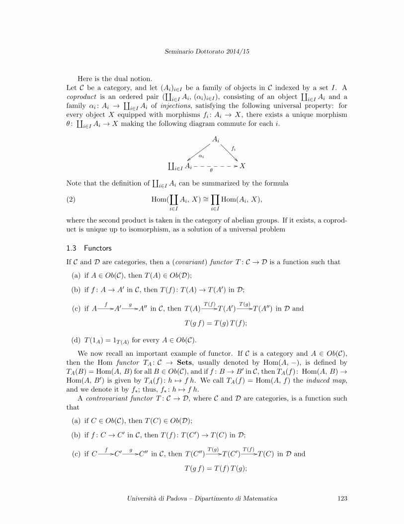
Seminario Dottorato 2014/15
Here is the dual notion.Let C be a category, and let (Ai)i∈I be a family of objects in C indexed by a set I. Acoproduct is an ordered pair (
∐i∈I Ai, (αi)i∈I), consisting of an object
∐i∈I Ai and a
family αi : Ai →∐i∈I Ai of injections, satisfying the following universal property: for
every object X equipped with morphisms fi : Ai → X, there exists a unique morphismθ :∐i∈I Ai → X making the following diagram commute for each i.
Ai
αi
fi
∐i∈I Ai θ
// X
Note that the definition of∐i∈I Ai can be summarized by the formula
(2) Hom(∐i∈I
Ai, X) ∼=∏i∈I
Hom(Ai, X),
where the second product is taken in the category of abelian groups. If it exists, a coprod-uct is unique up to isomorphism, as a solution of a universal problem
1.3 Functors
If C and D are categories, then a (covariant) functor T : C → D is a function such that
(a) if A ∈ Ob(C), then T (A) ∈ Ob(D);
(b) if f : A→ A′ in C, then T (f) : T (A)→ T (A′) in D;
(c) if Af //A′
g //A′′ in C, then T (A)T (f) //T (A′)
T (g) //T (A′′) in D and
T (g f) = T (g)T (f);
(d) T (1A) = 1T (A) for every A ∈ Ob(C).
We now recall an important example of functor. If C is a category and A ∈ Ob(C),then the Hom functor TA : C → Sets, usually denoted by Hom(A, −), is defined byTA(B) = Hom(A, B) for allB ∈ Ob(C), and if f : B → B′ in C, then TA(f) : Hom(A, B)→Hom(A, B′) is given by TA(f) : h 7→ f h. We call TA(f) = Hom(A, f) the induced map,and we denote it by f∗; thus, f∗ : h 7→ f h.
A controvariant functor T : C → D, where C and D are categories, is a function suchthat
(a) if C ∈ Ob(C), then T (C) ∈ Ob(D);
(b) if f : C → C ′ in C, then T (f) : T (C ′)→ T (C) in D;
(c) if Cf //C ′
g //C ′′ in C, then T (C ′′)T (g) //T (C ′)
T (f) //T (C) in D and
T (g f) = T (f)T (g);
Universita di Padova – Dipartimento di Matematica 123
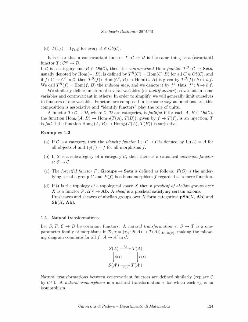
Seminario Dottorato 2014/15
(d) T (1A) = 1T (A) for every A ∈ Ob(C).
It is clear that a controvariant functor T : C → D is the same thing as a (covariant)functor T : Cop → D.If C is a category and B ∈ Ob(C), then the controvariant Hom functor TB : C → Sets,usually denoted by Hom(−, B), is defined by TB(C) = Hom(C, B) for all C ∈ Ob(C), andif f : C → C ′ in C, then TB(f) : Hom(C ′, B)→ Hom(C, B) is given by TB(f) : h 7→ h f .We call TB(f) = Hom(f, B) the induced map, and we denote it by f∗; thus, f∗ : h 7→ h f .
We similarly define functors of several variables (or multifunctors), covariant in somevariables and contravariant in others. In order to simplify, we will generally limit ourselvesto functors of one variable. Functors are composed in the same way as functions are, thiscomposition is associative and “identify functors” play the role of units.
A functor T : C → D, where C, D are categories, is faithful if for each A, B ∈ Ob(C),the function HomC(A, B) → HomD(T (A), T (B)), given by f 7→ T (f), is an injection; Tis full if the function HomC(A, B)→ HomD(T (A), T (B)) is surjective.
Examples 1.2
(a) If C is a category, then the identity functor 1C : C → C is defined by 1C(A) = A forall objects A and 1C(f) = f for all morphisms f .
(b) If S is a subcategory of a category C, then there is a canonical inclusion functorι : S → C.
(c) The forgetful functor F : Groups → Sets is defined as follows: F (G) is the under-lying set of a group G and F (f) is a homomorphism f regarded as a mere function.
(d) If U is the topology of a topological space X then a presheaf of abelian groups overX is a functor P : Uop → Ab. A sheaf is a presheaf satisfying certain axioms.Presheaves and sheaves of abelian groups over X form categories: pSh(X, Ab) andSh(X, Ab).
1.4 Natural transformations
Let S, T : C → D be covariant functors. A natural transformation τ : S → T is a one-parameter family of morphisms in D, τ = (τA : S(A)→ T (A))A∈Ob(C), making the follow-ing diagram commute for all f : A→ A′ in C:
S(A)
S(f)
τA // T (A)
T (f)
S(A′) τA′// T (A′).
Natural transformations between controvariant functors are defined similarly (replace Cby Cop). A natural isomorphism is a natural transformation τ for which each τA is anisomorphism.
Universita di Padova – Dipartimento di Matematica 124
Seminario Dottorato 2014/15
Natural transformations can be composed. If τ : S → T and σ : T → U are naturaltransformations, where S, T, U : C → D are functors, then define σ τ : S → U by (σ τ)A =σA τA, for all A ∈ Ob(C). It is easy to check that σ τ is a natural transformation (Rotman,Ex. 1.15).
For any functor S : C → D, define the identity natural transformation ωS : S → S bysetting (ωS)A : S(A) → S(A) to be the identity morphism 1S(A). The reader may checkthat a natural transformation τ : S → T is a natural isomorphism if and only if thereexists a natural transformation σ : T → S with σ τ = ωS and τ σ = ωT .
A functor S : C → D is an equivalence if there exists a functor T : D → C and naturalisomorphisms T S → 1C , S T → 1D.The following description of equivalence is often more closed at hand:
Proposition 1.3 A functor S : C → D is an equivalence if and only if it is full andfaithful, and every object of D is isomorphic to an object of the form S(C).
2 Abelian categories
2.1 Additive categories
An object A in a category C is called an initial object (respectively, a terminal object) if,for every object X ∈ C, there exists a unique morphism A → X (respectively, X → A).The reader may check that any two initial (respectively, terminal) objects in a categoryC, should they exist, are isomorphic and that this isomorphism is unique. A zero objectis an object that is both an initial object and a terminal object. If A is a zero objectin a category C, then Hom(A, A) is reduced to 0, and for any B ∈ Ob(C), Hom(A, B)(or Hom(B, A)) is reduced to 0. If A and A′ are zero objects, there exists a uniqueisomorphism of A to A′ (that is, the unique zero element of Hom(A, A′)). We will identifyall zero objects of C to a single one, denoted 0 by abuse of notation.
A category C is preadditive if
(a) Hom(A, B) is an (additive) abelian group for every A, B ∈ Ob(C);
(b) the distributive laws hold: given morphisms
Xa // A
f //g// B
b // Y,
where X and Y ∈ Ob(C), then
b (f + g) = b f + b g and (f + g) a = f a+ g a.
A preadditive category C is additive if the following two additional conditions holds:
(c) C has a zero object;
(d) C has finite products and finite coproducts.
Universita di Padova – Dipartimento di Matematica 125
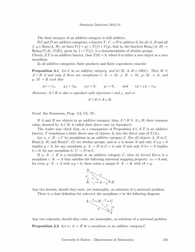
Seminario Dottorato 2014/15
The dual category of an additive category is still additive.If C and D are additive categories, a functor T : C → D is additive if, for all A, B and all
f, g ∈ Hom(A, B), we have T (f + g) = T (f) + T (g); that is, the function HomC(A, B)→HomD(T (A), T (B)), given by f 7→ T (f), is a homomorphism of abelian groups.Clearly, if T is an additive functor, then T (0) = 0, where 0 is either a zero object or a zeromorphism.
In all additive categories, finite products and finite coproducts coincide:
Proposition 2.1 Let C be an additive category, and let M, A, B ∈ Ob(C). Then M ∼=A u B if and only if there are morphisms i : A → M , j : B → M , p : M → A, andq : M → B such that
p i = 1A, q j = 1B, p j = 0, q i = 0, and i p+ j q = 1M .
Moreover, A uB is also a coproduct with injections i and j, and so
A uB ∼= A tB.
Proof. See Stenstrom, Prop. 3.2, Ch. IV.
If A and B are objects in an additive category, then A u B ∼= A t B; their commonvalue, denoted by A⊕B, is called their direct sum (or biproduct).
The reader may check that, as a consequence of Proposition 2.1, if T is an additivefunctor, T transforms a finite direct sum of objects Ai into the direct sum of T (Ai).
Let u, v : B → C be morphisms in an additive category C. For all objects A, D in C,Hom(A, B) and Hom(C, D) are abelian groups, and so u is monic if and only if u g = 0implies g = 0, for any morphism g : A → B in C; v is epic if and only if h v = 0 impliesh = 0, for any morphism h : C → D in C.
If u : A → B is a morphism in an additive category C, then its kernel Keru is amorphism ι : K → A that satisfies the following universal mapping property: u ι = 0 and,for every g : X → A with u g = 0, there exists a unique θ : X → K with i θ = g.
X
θ g
0
''K ι
// A u// B
Any two kernels, should they exist, are isomorphic, as solutions of a universal problem.There is a dual definition for cokernel, the morphism π in the following diagram:
A
0''
u // Bh
π // C
θY
Any two cokernels, should they exist, are isomorphic, as solutions of a universal problem.
Proposition 2.2 Let u : A→ B be a morphism in an additive category C.
Universita di Padova – Dipartimento di Matematica 126

Seminario Dottorato 2014/15
(a) If Keru exists, then u is monic if and only if Keru = 0.
(b) Dually, if Cokeru exists, then u is epic if and only if Cokeru = 0.
Proof. We refer to the diagrams in the definitions of kernel and cokernel. Let Keru beι : K → A, and assume that ι = 0. If g : X → A satisfies u g = 0, then the universalproperty of kernel provides a morphism θ : X → K with g = ι θ = 0 (because ι = 0).
Hence, u is monic. Conversely, if u is monic, consider Kι //
0//A
u //B . Since u ι = 0 =
u 0, we have ι = 0. The proof for epimorphisms and cokernels is dual.
It is immediate to show that any kernel is monic and any cokernel is epic.If ι is the kernel of some morphism and if Coker ι exists, then ι = Ker(Coker ι). Indeed,
let ι : K → A be the kernel of u : A→ B. Then u ι = 0 implies that u factors over Coker ι.If now ξ : X → A is any morphism such that Coker ι ξ = 0, then it follows that u ξ = 0,and ξ factors uniquely over Keru = ι. Therefore, ι is the kernel of Coker ι.
Let f : A→ B be a morphism in an additive category C, and assume that its cokernelCoker f : B → C exists. Then its image is Im f = Ker(Coker f). In more suggestive
notation, Im(Af→ B) = Ker(CokerA
f→ B). We denote Ker(Coker f) by Im f . Dually,one defines the notion of coimage.
2.2 Abelian categories
An abelian category is an additive category C that satisfies the following two additionalconditions (which are self-dual):
(e) Any morphism admits a kernel and a cokernel;
(f) Let u be a morphism in C. Then the canonical morphism u : Coimu → Imu is anisomorphism.
Let us show that given a morphism u : A → B in an additive category C, there isa canonical morphism u : Coimu → Imu. Let u : A → B, then there is a canonicalfactorization as indicated by the commutative diagram
Keru // Au //
λ
B //
µ
Cokeru
Coimuu// Imu
where u is obtained as follows: (Cokeru)u = 0 implies that u factors as u = µα (by theuniversal property of the kernel), for some α : A → Imu; then µα Keru = u Keru = 0implies that αKeru = 0, since µ, being a kernel, is monic. Therefore, α factors as α = uλ(by the universal property of the cokernel).
If C is an abelian category and B is a subcategory of C which is also abelian, then B issaid to be an abelian subcategory if the inclusion functor B → C is exact.
Universita di Padova – Dipartimento di Matematica 127
Seminario Dottorato 2014/15
If C is an abelian category, then the entire formalism of diagrams of homomorphismsbetween abelian groups can be carried over if we replace homomorphisms by morphisms inC, insofar as we are looking at properties of finite type, i.e. not involving infinite productsor coproducts. We content ourselves here with indicating a few particularly importantfacts. Note that the axiom (6) is equivalent to the following one:
(6’) Every morphism u has a factorization as u = ιπ, where π is a cokernel and ι is akernel.
Indeed, it is obvious that (6) implies (6′). Conversely, let C be a category satisfying (1)-(5) and (6’). If u factors as in (6’), then π = Coimπ = Coker(Kerπ) and ι = Im ι =Ker(Coker ι). But Kerπ = Keru since ι is a monomorphism, and similarly Coker ι =Cokeru. We conclude that Coker(Keru) = Ker(Cokeru), that is Coimu = Imu.
For the rest of this section we assume that C is abelian. The previous discussion shows:
Proposition 2.3 Let u be a morphism in C.
(a) If u is both a monomorphism and an epimorphism, then u is an isomorphism;
(b) If u is a monomorphism, then u = Ker(Cokeru);
(c) If u is a epimorphism, then u = Coker(Keru).
A sequence . . . //Ci−1αi−1 //Ci
αi //Ci+1αi+1 // // . . . is exact at Ci if Imαi−1 = Kerαi
(equals as subobjects of Ci). The whole sequence is exact if it is exact at each Ci.Let T : C → C′ be a (covariant) functor, where C′ is an abelian category. We say that T
is left exact (respectively, right exact) if T transforms any exact sequence 0 //A //B //C(respectively, A //B //C //0) into an exact sequence 0 //T (A) //T (B) //T (C)(respectively, T (C) //T (B) //T (A) //0). T is called an exact functor if it is bothleft exact and right exact; that is, T transforms any short exact sequence 0 //A //B //C //0into an exact sequence 0 //T (A) //T (B) //T (C) //0. If T is a controvariantfunctor, we say that T is left exact (respectively, right exact) if T has the correspondingproperty as a covariant functor Cop → C′.The composite of left exact, right exact, exact covariant functors is of the same type.As a significant example, we note that Hom(−, −) is an additive bifunctor on Cop×C, withvalues in Ab, controvariant in the first argument and covariant in the second argument,and left exact with respect to each argument.
Let C ∈ Ob(C), (Ci)i∈I a family of subobjects of C, and assume that the coproduct∐i∈I Ci exists. The monomorphisms Ci → C induce a morphism α :
∐i∈I Ci → C. The
image of α is called the sum of the subobjects Ci and it is denoted by∑
i∈I Ci. If α isa monomorphism, then it induces an isomorphism
∐i∈I Ci
∼=∑
i∈I Ci, and in this casethe sum is called direct sum. Dually, the epimorphisms C → C/Ci induce a morphismβ : C →
∏i∈I C/Ci (when the product exists). The kernel of β is the intersection of the
subobjects Ci and it is denoted by⋂i∈I Ci.
Universita di Padova – Dipartimento di Matematica 128
Seminario Dottorato 2014/15
Examples 2.4
(a) R-Mod is abelian, for any ring R. In fact, it can be shown that any small abeliancategory is equivalent to a full subcategory of such a category of modules (Mitchell’sembedding theorem). In particular:
(b) Ab is abelian.
(c) Groups is not abelian, as it is not additive.
(d) The full subcategory of Ab of all finitely generated abelian groups is an abeliancategory, as is the full subcategory of all torsion abelian groups.
(e) The full subcategory of Ab of all torsion-free abelian groups is not an abelian cate-gory, for there are morphisms having no cokernel; for example, the inclusion 2Z→ Zhas cokernel Z/2Z, which is not torsion-free.
(f) pSh(X, Ab) and Sh(X, Ab) are abelian categories. More generally, if C is anabelian category, then pSh(X, C) and Sh(X, C) are abelian.
(g) If C is abelian, then its opposite category Cop is abelian. So, a theorem using onlythe axioms in its proof is true in every abelian category; moreover, its dual is also atheorem in every abelian category, and its proof is dual to the original proof.
3 Derived categories
3.1 The category of cochain complexes and the homotopy category
In this section we let C be an additive category. A complex X• = (Xk, dkX) over C is asequence of objects Xk and morphisms dkX : Xk → Xk+1 (k ∈ Z):
. . . // Xk−1dk−1X // Xk
dkX // Xk+1 // . . .
such that dk+1X dkX = 0 for all k ∈ Z. A complex is bounded below if Xk = 0 for all but
finitely many k < 0. It is bounded above if Xk = 0 for all but finitely many k > 0. Itis bounded if it is bounded below and bounded above. We denote by Ch(C) the additivecategory of complexes and by Ch∗(C) (∗ = b, +, −) the full additive subcategory of Ch(C)consisting of bounded complexes (resp. bounded below, bounded above). We may considerC as a full subcategory of Chb(C) by identifying each object X of C with the complex. . . //0 //X //0 // . . . “concentrated in degree 0”, where X stands in degree 0.
Let X ∈ Ob(Ch(C)) and p ∈ Z. The shift functor is defined by
(X[p])n = Xn+p, dnX[p] = (−1)pdn+pX
and if f : X → Y is a morphism in Ch(C), then
(f [p])n = fn+p.
Universita di Padova – Dipartimento di Matematica 129
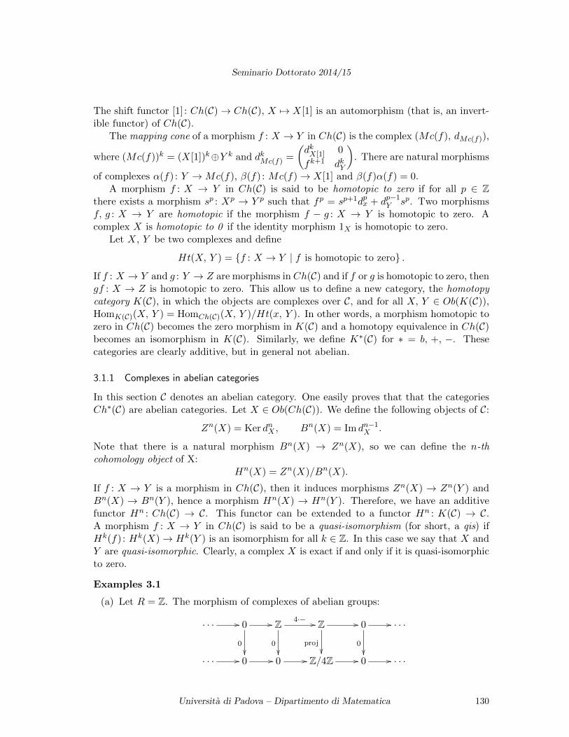
Seminario Dottorato 2014/15
The shift functor [1] : Ch(C)→ Ch(C), X 7→ X[1] is an automorphism (that is, an invert-ible functor) of Ch(C).
The mapping cone of a morphism f : X → Y in Ch(C) is the complex (Mc(f), dMc(f)),
where (Mc(f))k = (X[1])k⊕Y k and dkMc(f) =
(dkX[1] 0
fk+1 dkY
). There are natural morphisms
of complexes α(f) : Y →Mc(f), β(f) : Mc(f)→ X[1] and β(f)α(f) = 0.A morphism f : X → Y in Ch(C) is said to be homotopic to zero if for all p ∈ Z
there exists a morphism sp : Xp → Y p such that fp = sp+1dpx + dp−1Y sp. Two morphisms
f, g : X → Y are homotopic if the morphism f − g : X → Y is homotopic to zero. Acomplex X is homotopic to 0 if the identity morphism 1X is homotopic to zero.
Let X, Y be two complexes and define
Ht(X, Y ) = f : X → Y | f is homotopic to zero .
If f : X → Y and g : Y → Z are morphisms in Ch(C) and if f or g is homotopic to zero, thengf : X → Z is homotopic to zero. This allow us to define a new category, the homotopycategory K(C), in which the objects are complexes over C, and for all X, Y ∈ Ob(K(C)),HomK(C)(X, Y ) = HomCh(C)(X, Y )/Ht(x, Y ). In other words, a morphism homotopic tozero in Ch(C) becomes the zero morphism in K(C) and a homotopy equivalence in Ch(C)becomes an isomorphism in K(C). Similarly, we define K∗(C) for ∗ = b, +, −. Thesecategories are clearly additive, but in general not abelian.
3.1.1 Complexes in abelian categories
In this section C denotes an abelian category. One easily proves that that the categoriesCh∗(C) are abelian categories. Let X ∈ Ob(Ch(C)). We define the following objects of C:
Zn(X) = Ker dnX , Bn(X) = Im dn−1X .
Note that there is a natural morphism Bn(X) → Zn(X), so we can define the n-thcohomology object of X:
Hn(X) = Zn(X)/Bn(X).
If f : X → Y is a morphism in Ch(C), then it induces morphisms Zn(X) → Zn(Y ) andBn(X) → Bn(Y ), hence a morphism Hn(X) → Hn(Y ). Therefore, we have an additivefunctor Hn : Ch(C) → C. This functor can be extended to a functor Hn : K(C) → C.A morphism f : X → Y in Ch(C) is said to be a quasi-isomorphism (for short, a qis) ifHk(f) : Hk(X)→ Hk(Y ) is an isomorphism for all k ∈ Z. In this case we say that X andY are quasi-isomorphic. Clearly, a complex X is exact if and only if it is quasi-isomorphicto zero.
Examples 3.1
(a) Let R = Z. The morphism of complexes of abelian groups:
· · · // 0 //
0
Z 4·− //
0
Z //
proj
0 //
0
· · ·
· · · // 0 // 0 // Z/4Z // 0 // · · ·
Universita di Padova – Dipartimento di Matematica 130
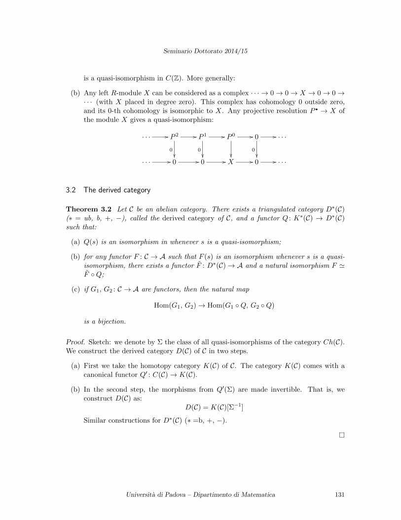
Seminario Dottorato 2014/15
is a quasi-isomorphism in C(Z). More generally:
(b) Any left R-module X can be considered as a complex · · · → 0→ 0→ X → 0→ 0→· · · (with X placed in degree zero). This complex has cohomology 0 outside zero,and its 0-th cohomology is isomorphic to X. Any projective resolution P • → X ofthe module X gives a quasi-isomorphism:
· · · // P 2 //
0
P 1 //
0
P 0 //
0 //
0
· · ·
· · · // 0 // 0 // X // 0 // · · ·
3.2 The derived category
Theorem 3.2 Let C be an abelian category. There exists a triangulated category D∗(C)(∗ = ub, b, +, −), called the derived category of C, and a functor Q : K∗(C) → D∗(C)such that:
(a) Q(s) is an isomorphism in whenever s is a quasi-isomorphism;
(b) for any functor F : C → A such that F (s) is an isomorphism whenever s is a quasi-isomorphism, there exists a functor F : D∗(C)→ A and a natural isomorphism F 'F Q;
(c) if G1, G2 : C → A are functors, then the natural map
Hom(G1, G2)→ Hom(G1 Q, G2 Q)
is a bijection.
Proof. Sketch: we denote by Σ the class of all quasi-isomorphisms of the category Ch(C).We construct the derived category D(C) of C in two steps.
(a) First we take the homotopy category K(C) of C. The category K(C) comes with acanonical functor Q′ : C(C)→ K(C).
(b) In the second step, the morphisms from Q′(Σ) are made invertible. That is, weconstruct D(C) as:
D(C) = K(C)[Σ−1]
Similar constructions for D∗(C) (∗ =b, +, −).
Universita di Padova – Dipartimento di Matematica 131
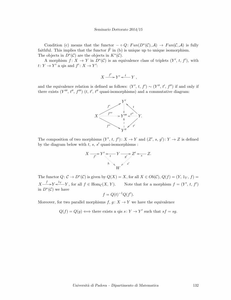
Seminario Dottorato 2014/15
Condition (c) means that the functor − Q : Fun(D∗(C),A) → Fun(C,A) is fullyfaithful. This implies that the functor F in (b) is unique up to unique isomorphism.The objects in D∗(C) are the objects in K∗(C).
A morphism f : X → Y in D∗(C) is an equivalence class of triplets (Y ′, t, f ′), witht : Y → Y ′ a qis and f ′ : X → Y ′:
Xf ′ // Y ′ Y
too ,
and the equivalence relation is defined as follows: (Y ′, t, f ′) ∼ (Y ′′, t′, f ′′) if and only ifthere exists (Y ′′′, t′′, f ′′′) (t, t′, t′′ quasi-isomorphisms) and a commutative diagram:
Y ′
X
f ′77
f ′′′ //
f ′′ ''
Y ′′′ Y.t′′oo
t′
t
aa
Y ′′
OO
The composition of two morphisms (Y ′, t, f ′) : X → Y and (Z ′, s, g′) : Y → Z is definedby the diagram below with t, s, s′ quasi-isomorphisms :
Xf ′// Y ′
h
Yt
oog′// Z ′
s′~~
Z.soo
W
The functor Q : C → D∗(C) is given by Q(X) = X, for all X ∈ Ob(C), Q(f) = (Y, 1Y , f) =
Xf //Y Y
1Yoo , for all f ∈ HomC(X, Y ). Note that for a morphism f = (Y ′, t, f ′)in D∗(C) we have
f = Q(t)−1Q(f ′).
Moreover, for two parallel morphisms f, g : X → Y we have the equivalence
Q(f) = Q(g)⇐⇒ there exists a qis s : Y → Y ′ such that sf = sg.
Universita di Padova – Dipartimento di Matematica 132
Seminario Dottorato 2014/15
References
[1] P. Gabriel, Des categories abeliennes. Bulletin de la Societe Mathematique de France 90(1962), 323–448.
[2] A. Grothendieck, Sur quelques points d’algebre homologique. Tohoku Mathematical Journal,Second Series 9.2 (1957), 119–183.
[3] M. Kashiwara and P. Schapira, “Categories and sheaves”. Grundlehren 332, Springer, 2006.
[4] B. Keller, Deriving DG categories. Ann. Sci. Ecole Norm. Sup. (4) 27 (1994), no. 1, 63–102.
[5] B. Keller, Derived categories and tilting. Handbook of tilting theory, London Math. Soc.Lecture Note Ser., vol. 332, Cambridge Univ. Press, Cambridge, 2007, pp. 49–104.
[6] A. Neeman, The Grothendieck duality theorem via Bousfields techniques and Brown repre-sentability. Journal of the American Mathematical Society 9 (1996), no. 1, 205–236.
[7] A. Neeman, “Triangulated categories”. Princeton, NJ: Princeton University Press, 2001.
[8] J. L. Verdier, Categories Derivees Quelques resultats (Etat 0). In “Cohomologie etale” (P.Deligne ed.), Lecture Notes in Mathematics 569, Springer Berlin Heidelberg, 1977, pp. 262–311.
Universita di Padova – Dipartimento di Matematica 133
Seminario Dottorato 2014/15
Why should people in
approximation theory care
about (pluri-)potential Theory?
Federico Piazzon (∗)
Abstract. We give a summary of results in (pluri-)potential theory that naturally come into playwhen considering classical approximation theory issues both in one and (very concisely) in severalcomplex variables. We focus on Fekete points and the asymptotic of orthonormal polynomials forcertain L2 counterpart of Fekete measures.
1 One variable case
1.1 Interpolation and Fekete Points
Let K ⊂ C be a compact set such that C∞\K is connected and f : K → C be a continuousfunction that is holomorphic in the interior of K, then Mergelyan Theorem ensures theexistence of sequences of polynomials uniformly approximating f on K.
Two reasonable questions are whether we can compute such a sequence by interpolationor not, and how the interpolation nodes should be chosen. It turns out that these questionsbecome much more difficult when suitably translated in the several variables context.
From here on we suppose K to be a polynomial determining set, that is if a polynomialvanish on K then it is the zero polynomial. If we consider the monomial basis zjj=1,2,...,k
for the space Pk of polynomials of degree at most k and we pick k+1 distinct points zk :=(z0, z1, . . . , zk) ∈ Kk+1 the interpolation problem can be written as V DMk(z0, . . . , zk)c =(f(z0), . . . , f(zk))
t where c ∈ Ck+1 and
VDMk
(z0, . . . , zk) := [zji ]i,j=0,...,k
is the Vandermonde Matrix. Notice that for each k+1-tuple of distinct points det VDMk(zk) 6=0 so the problem is well posed.
(∗)Ph.D. course, Universita di Padova, Dip. Matematica, via Trieste 63, I-35121 Padova, Italy; E-mail:. Seminar held on June 24th, 2015.
Universita di Padova – Dipartimento di Matematica 134
Seminario Dottorato 2014/15
It is a classical result that the norm of the operator Ik : (C (K), ‖ · ‖K)→(Pk, ‖ · ‖K
)is the Lebesgue Constant Λk := maxz∈K
∑km=0 |lm,k(z)|, where lm,k(z) :=
det VDMk(z0,...,zl−1,zl,...,zk)det VDMk(z0,...,zk) .
Minimizing Λk(zk) is an extremely hard task so one can consider the simplified problemof maximizing |det VDM(zk)|, though it is still a very hard one.
Definition 1.1 (Fekete Points) Let K ⊂ C be a compact set and zk := (z0, . . . , zk) ∈Kk+1. If we have |det VDMk(zk)| = maxζ∈Kk+1 | det VDMk(ζ)|, then zk is said to be aFekete array of order k, its elements are said Fekete points.
The relevance of Fekete points is easy to see: one has Λk(F k) ≤ k + 1 for any Feketearray F k; moreover notice that in general F k is not unique.
An interesting property of Vandermonde determinants is that for any array of pointszk we have
|det VDMk
(zk)| =∏i<j≤k
|zi − zj |
that is the product of their distances; this is one of the main points in connectinginterpolation with logarithmic potential theory. We introduce the number dk(K) :=
|VDMk(zk)|1/(k2) for one (thus any) Fekete array zk of order k. In analogy with the
case k = 0, dk(K) is called k-th diameter of K, it is a decreasing positive sequence, itslimit d(K) is called transfinite diameter of K.
Example 1.2 (Fekete points on the unit disc) Let D be the unit circle. Take any setof distinct points z = z0, . . . , zk and consider the determinant of the matrix V (z) :=VDMk(z). We have
‖V:,j(z)‖2 =
∥∥∥∥∥∥∥∥∥
zj0zj1...
zjk
∥∥∥∥∥∥∥∥∥
2
=√k + 1, for any j = 0, 1, . . . k.
Therefore Hadamard Inequality for determinants implies | det VDMk(z)| ≤∏kj=0 ‖V:,j(z)‖2 =
(k+ 1)k+12 . This upper bound is achieved if and only if the columns of V (z) are orthonor-
mal and this condition is satisfied for z a set of k+1 roots of unity. Therefore 2iπjk+1j=0,...,k
is a Fekete set for D.
1.2 Logarithmic Potential Theory
It is customary to introduce the differential operators d := ∂ + ∂ and dc := i(∂ − ∂) suchthat (passing to real coordinates) one has ∆ = 2i∂∂ = ddc.
We recall that using the Green Identity it is possible to show that E(z) := 12π log |z| is
a fundamental solution for the Laplacian, i.e., ddcE(z) = δ0 in the sense of distributions.We also recall that a real valued function u ∈ C 2 on a domain Ω is said to be harmonicif ∆u = 0 in Ω. A upper semi-continuous function v is said to be subharmonic in Ω if forany open relatively compact subset Ω1 ⊂ Ω and any harmonic function u on Ω such that
Universita di Padova – Dipartimento di Matematica 135
Seminario Dottorato 2014/15
v ≤ u on ∂Ω1 we have v ≤ u on Ω1. It follows that, given any compactly supported finiteBorel measure µ, the function
Uµ(z) := µ ∗ E(z) =
∫log
1
|z − ζ|dµ(ζ),
said the logarithmic potential of µ, is a superharmonic function (i.e. −Uµ is subharmonic)on C and in particular harmonic in C \ suppµ, moreover we have ddc Uµ = µ.
To the Laplace operator is naturally attached an energy minimization problem; werefer the reader to [21], [23] and [22] for details.
Problem 1.1 (Logarithmic Energy Minimization) Let K be a compact subset of C, min-imize
(LEM) I[µ] :=
∫ ∫log
1
|z − ζ|dµ(ζ)dµ(z) =
∫Uµ(z)dµ(z),
among µ ∈ M1(K), the set of Borel probability measures on K endowed with the weak∗
topology.
We notice that if we consider the electrostatic interaction between k+1 unitary charges
in the plan, the force acting on the i-th particle is∑
j 6=i(xi,xj ,yi−yj)|zi−zj |2 = −∇Uµ, where µ
denotes the uniform probability measure associated to the charges distribution. The elec-trostatic energy associated to this charges distribution is precisely Uµ =
∑i 6=j∑
log 1|zi−zj | ,
this minimization problem is very close to (LEM), we will see that in particular (LEM)is, in a suitable sense, its limit.
It turns out that I[·] is a lower semi-continuous functional on a locally compact space,one can use the Direct Methods of Calculus of Variation to prove that two situations mayoccur. Either I[µ] = +∞ for all µ ∈ M1(K), either there exists a unique minimizer thatis the equilibrium measure of K and is usually denoted by µK .
In the latter case one has UµK (z) = − log c(K) − gK(z), where gK := GC∞\K is thegeneralized (e.g. possibly not continuous) Green function with logarithmic pole at ∞ forthe complement of K. The number c(K) called logarithmic capacity of K and is defined asc(K) := exp(− infµ∈M1(K) I[µ]), thus is non zero precisely when the minimization problemis well posed. It turns out that UµK (z) = − log c(K) quasi everywhere on K, that is forany z ∈ K but for set of zero logarithmic capacity.
Sets of zero capacity are, roughly speaking, too small for logarithmic potential theory,they are termed polar and it can been shown that c(K) = 0 if and only if K is the −∞set of some subharmonic function defined in a neighbourhood of K.
The following result is due to Szego, Leja and Fekete.
Theorem 1.3 (Fundamental Theorem of Logarithmic Potential Theory) Let K ⊂ C be acompact non polar set, we have
c(K) = d(K).
Therefore, for any sequence of Fekete arrays F k, setting µk := 1k+1
∑kj=0 δF jk
, we have
µk* µK .
Universita di Padova – Dipartimento di Matematica 136
Seminario Dottorato 2014/15
Moreover locally uniformly on C \K we have
limk−Uµk(z) := lim
k
1
k + 1log
k+1∏j=0
|z − F jk | = gK(z)− log c(K) = −UµK .
The proof is based on lower semi-continuity and strict convexity of the energy func-tional and on the extremal property of Fekete points. Moreover the result holds truefor any sequence of so called asymptotically Fekete arrays that is, arrays Lk such that
limk |VDMk(Lk)|1/(n2) = d(K).
1.3 Back to Approximation
Other deep connections between interpolation and logarithmic potential theory are givenby the following two results. We recall that a compact set K is said to be regular if gK isa continuous function.
Theorem 1.4 (Bernstein Walsh [25]) Let K be a compact polynomially determining nonpolar set, then we have
gK(z) = lim supζ→z
(1
deg plog+ |p(ζ)|, ‖p‖K ≤ 1
).
Moreover
(Bernstein Wals Ineq.) |p(z)| ≤ ‖p‖K exp(deg p gK(z)) ∀p ∈P(C).
The approximation theorem comes as an application of Hermite reminder formula andthe previous theorem.
Theorem 1.5 (Bernstein-Walsh [25]) Let K ⊂ C be a compact regular polynomially convexnon polar set and f : K → C be a bounded function. Let dk(f,K) := inf‖f − p‖K : p ∈Pk, then for any real number R > 1 the following are equivalent
(1) limk dk(f,K)1/k < 1/R
(2) f is the restriction to K of f ∈ hol(DR), where DR := gK < logR.
1.4 L2 theory
We want to show that some analogues of results for Fekete points (that are L∞ maximizers,in some sense) holds for particular measures in a L2 fashion.
Definition 1.6 (Bernstein Markov Measures) Let K ⊂ C be a compact set and µ be aBorel measure such that suppµ ⊆ K, assume that
lim supk
(‖pk‖K‖pk‖L2
µ
)1/deg(pk)
≤ 1,
Universita di Padova – Dipartimento di Matematica 137
Seminario Dottorato 2014/15
for any sequence of non zero polynomials pk. Then we say that (K,µ) has the BernsteinMarkov property, BMP for short, or equivalently µ is a Bernstein Markov measure on K.
Example 1.7 We claim that dµ := 12πdθ is a Bernstein Markov measure for S1. To show
that, one first notice that the monomials (up to degree k) are a orthonormal basis of(Pk, 〈·; ·〉L2
µ
). Therefore, for any p ∈Pk we have
|p(z)| =
∣∣∣∣∣∣k∑j=0
〈p; zj〉L2µzj
∣∣∣∣∣∣ ≤ ‖p‖L2µ
k∑j=0
|zj |21/2
≤√k + 1‖p‖L2
µ,
hence lim supk
(‖pk‖K‖pk‖L2
µ
)1/ deg(pk)
≤ lim supk(k + 1)1/2k = 1.
Bernstein Markov measures on a given K are in general a very large set as the followingsufficient condition shows. For a exhaustive treatment of regular measures (e.g. a weakenedversion of Bernstein Markov property) the reader is referred to [24]; generalization to theCn version can be found in [5]. A survey with further development is [10].
Theorem 1.8 (Sufficient condition for BMP [24]) Let K be a compact non polar regularset and µ a Borel measure such that suppµ = K, assume that there exists a positivenumber t > 0 such that
(1) limr→0+
c(z ∈ K : µ(B(z, r)) ≥ rt
)= c(K).
Then (K,µ) satisfies the Bernstein Markov property.
Finding necessary condition is a relevant open question in the general theory of or-thogonal polynomials, a necessary condition was stated as a conjecture by Erdos.
The first interest on BMP is from the approximation point of view. Let us take aorthonormal system qjj=0,1,... for P, then each Pk is a Reproducing Kernel Hilbert
Space, being Kµk (z, ζ) :=
∑kj=0 qj(z)qj(ζ) the kernel. We denote by Bµ
k (z) the diagonal of
the kernel, say the Bergman Function Bµk (z) = Kµ
k (z, z) =∑k
j=0 |qj(z)|2. It is not hardto see that the Bergman function represent the worst possible case for the l.h.s. of the
definition of BMP, that is supdeg p≤k‖p‖K‖p‖
L2µ
=√‖Bµ
k ‖K .
We consider natural the projection operator Lµk :(C 0(K), ‖ · ‖K
)→(Pk, ‖ · ‖K
)defined by embedding the two spaces in L2
µ, Lµk [f ](z) :=
∑kj=0〈f, qj〉qj(z). It follows that
‖Lµk [f ]‖K ≤
k∑j=0
|〈f, qj〉|21/2
∥∥∥∥∥∥∥ k∑j=0
|qj(z)|21/2
∥∥∥∥∥∥∥K
≤ ‖f‖L2µ
√‖Bµ
k (z)‖K ≤ ‖f‖K√µ(K)‖Bµ
k (z)‖K .
Universita di Padova – Dipartimento di Matematica 138
Seminario Dottorato 2014/15
Therefore we have ‖Lµk‖ ≤√µ(K)‖Bµ
k (z)‖K . This can be used to bound the error of poly-
nomial approximation by least square projection, let pk be the best uniform polynomialapproximation of degree at most k to f
‖f − Lµk [f ]‖K = ‖f − pk + pk − Lµk [f ]‖K
≤ dk(f,K) + ‖Lµk [f − pk]‖K ≤ dk(f,K)
(1 +
√µ(K)‖Bµ
k (z)‖K).
This allows us to state a version of the Bernstein Walsh Lemma in a L2 fashion forBernstein Markov measures.
Theorem 1.9 (Bernstein Walsh L2 version [17]) Let K be a compact polynomially convexregular non polar set and µ a Borel probability measure such that suppµ = K satisfyingthe Bernstein Markov property. Then the following are equivalent.
(1) limk dk(f, µ)1/k < 1/R
(2) f is the restriction to K of f ∈ hol(DR), where DR := gK < logR.
Here limk dk(f, µ) is the error of best L2µ polynomial approximation to f of degree not
greater than k.There are other interesting analogies between BM measures and measures associated
to Fekete points. First we notice that if we pick a Fekete array Fk for K and we computethe squares of the modulus of the Vandermonde determinant on such points we can rewriteit as a L2 norm w.r.t. the associated Fekete measure µk, that is(2)
(k(k+1))!| det VDM(Fk)|2 =
∫. . .
∫| det VDM(ζ0, . . . , ζk)|2dµk(ζ0) . . . dµk(ζk) := Zk(µk),
notice that the right hand side can be generalized to any measure on E. On the otherhand if we perform the Gram-Schmidt ortogonalization of the Vandrmonde matrix onethe right hand side of (2) we obtain (up to a normalizing constant (k(k+1))!) the productof L2
µ norms of the monic orthonormal polynomials relative to µ and this is precisely the
determinant of the Gram-matrix Gµkk w.r.t.(Pk, ‖ · ‖L2
µk
)in the standard basis, that is
Gµkk = [〈zizj〉L2µk
]i,j .
This observation leads to a generalization of asymptotically Fekete points to any mea-sure, namely µ ∈M1(E) is asymptotically Fekete for E if limk Zk(µ,E)1/(k(k+1)) = d(E).
The following result, despite a not very difficult proof is fundamental, especially inmore general contexts: Bernstein Markov measures are asymptotically Fekete; see [8, 6].
Proposition 1.1 Let K be a compact non polar set and µ a Borel probability measuresuch that suppµ ⊂ K satisfying the Bernstein Markov property. We have
limk
(∫. . .
∫| det VDM(ζ0, . . . , ζk)|2dµ(ζ0) . . . dµ(ζk)
) 1k(k+1)
= limk
[(k(k + 1))! detGµk
] 1k(k+1) = d(K).
Universita di Padova – Dipartimento di Matematica 139
Seminario Dottorato 2014/15
Morally speaking, Fekete points are L∞ maximizers, while BM measures are L2 max-imizers.
Also we have that other interesting properties of Fekete points can be translated inthis fashion.
Theorem 1.10 Let K be a compact non polar set and µ a Borel probability measure suchthat suppµ ⊂ K satisfying the Bernstein Markov property. We have
i) limk1
2k(k+1) logBµk (z) = gK(z) point-wise, locally uniformly if K is regular.
ii) limkBµk
k(k+1)µ = µK in the weak∗ sense.
Notice that for Fekete measures Bµkk is the sum of the squared modulus of Lagrange
polynomials andBµkk
k(k+1) ≡ 1 on the support of µk.There are other applications of Bernstein Markov measures and potential theory tools
concerning for instance random polynomials ensambles generalizing the classical result onKac polynomials and asymptotic of zeroes of orthogonal polynomials; see for instance [11],[5], [9].
2 Several Variables Case
The extension of what we saw in the case of one complex variable is much more difficultand technical, but still the most of the relation in the previous section have their scvcounterpart, provided a correct ”translation”.
The first difficulty is in defining the n-dimensional transfinite diameter for a givencompact set, in particular showing the existence of the limit and its independence by theordering of the monomial basis. The solution has been given by Zaharjuta [26] by a so-phisticate procedure comparing the k-th diameter with certain integral mean of directionalChebyshev constants.
The second problem is that logarithmic energy is not related to maximization of Van-dermonde determinants when n > 1. As a consequence, subharmonic functions are nomore the ”correct space” to look at; they are replaced in this context by plurisubharmonicones.
Plurisubharmonic functions, PSH for short, are upper semi continuous functions beingsubharmonic along each complex line. This property is invariant under any holomorphicmapping, moreover there is a differential operator (the complex Monge Ampere) playinga role with PSH function similar to the one of Laplacian with respect to subharmonicfunctions in C.
Let u ∈ PSH(Cn) ∩ C 2, then one can consider the continuous (1, 1) form ddc u,
ddc u :=n∑i=1
2i∂2
∂zi∂zju(z)dzi ∧ dzj
Universita di Padova – Dipartimento di Matematica 140
Seminario Dottorato 2014/15
and then take the wedge powers of it
(ddc u)n := ddc u ∧ · · · ∧ ddc u = det[∂2
∂zi∂zju(z)]i,jdVn,
where dVn is the standard volume form on Cn.It is a classical result that ddc u can be defined as a positive current (i.e., an element of
the dual of test forms) for any PSH function and, due to the seminal works of Bedford andTaylor [1] [2], for locally bounded PSH function the operator (ddc u)n is well defined as apositive Borel measure. This extension is termed the generalized complex Monge Ampereoperator, Pluripotential Theory is the study of plurisubharmonic functions and MongeAmpere operator; we refer the reader to [15] for a detailed treatment of the subject.
In this context the role of Harmonic function is replaced by maximal plurisubharmonicfunctions that are defined requiring precisely the domination property that harmonicfunctions enjoy with respect to subharmonic functions in C; they are characterized by(ddc u)n = 0 in the sense of measures on the given domain. We denote by L(Cn) the classof plurisubharmonic functions with logarithmic pole at infinity, the Dirichlet problem forthe Monge Ampere operator
(ddc u)n = 0 in Cn \Ku =q.e. 0 on K,u ∈ L(Cn) ∩ L∞loc
enjoys the role of the Dirichlet problem for the Laplacian in C, its solution V ∗K is calledplurisubharmonic extremal function or, by analogy, pluricomplex Green function. BeingV ∗K representable, precisely as gK , with the (upper-semicontinuous regularization of the)upper envelope of function v in L(Cn) such that v ≤ 0 on K.
V ∗K(z) := lim supζ→z
VK(ζ)
VK(ζ) := supu(ζ), u ∈ L(Cn), u|K ≤ 1.
Again, as in the one dimension, one has ∆gK = µK here one has a pluripotential equilibriummeasure µK := (ddc V ∗K)n, thus it is supported on K by definition.
Pluripotential theory has analogies with potential theory but also differences, first theMonge Ampere operator if fully non linear, there is no notion of potential, a suitableenergy functional has been found only recently and there is no direct connection betweenpolynomials and finitely supported measures. However there are plenty of good news aswell.
First, the (Bernstein Wals Ineq.) goes precisely to Cn replacing gK by V ∗K , due tothat and a density result one has the scv counterpart (again replacing gK by V ∗K) of theBernstein Walsh Lemma 1.4, usually referred as the Bernstein Walsh Siciak Theorem.
For years the extension of the asymptotic property of Fekete points to Cn has been onlyconjectured. The work (see [4], [3]) of Berman Boucksom and Nymstrom finally provedthat, despite the strong differences between potential and pluripotential theory, one hasthe same L∞ and L2 asymptotic results. More precisely, for a non pluri-polar (i.e., notcontained in the −∞ set of a plurisubharmonic function) compact set K the followingholds.
Universita di Padova – Dipartimento di Matematica 141
Seminario Dottorato 2014/15
(a) Fekete measures for K converge weakly∗ to µK .
(b) The same remains true for any sequence of asymptotically Fekete arrays.
(c) For any Bernstein Markov measure µ limkBµk
dim Pk(Cn)µ = µK .
(d) For any Bernstein Markov measure µ limk12k logBµ
k = V ∗K locally uniformly if K isL-regular, e.g. V ∗K is continuous.
Moreover, the sufficient condition for the Bernstein Markov property can be translatedto Cn by replacing the logarithmic capacity by a non linear ”local” (e.g., relative to aopen hold all set) capacity associated with the Monge Ampere operator, say the relativecapacity ; see [7].
3 A discrete approach
Admissible meshes, shortly AM, are sequences Ak of finite subsets of a given compactset K such that
• there exists a positive real constant C such that for any p ∈Pk we have
maxK|p| ≤ C max
Ak|p|.
• CardAk increase at most polynomially.
They have been first introduced [14] as good sampling sets for uniform polynomial ap-proximation by discrete least squares. The construction of such subsets has been studiedfor several cases, with emphasis in holding the cardinality growth rate; see for instances[12, 18, 20, 16].
Let associate the uniform probability measure µk to Ak, then we can see that, pickingan orthonormal system q1, . . . , qNk of Pk we have√√√√‖ Nk∑
j=1
|qj |‖K =√‖Bµk
k ‖K ≤ C supp∈Pk
‖p‖Ak‖p‖L2
µk
≤ C√
CardAk.
As a consequence the error of uniform polynomial approximation by DLS on an AM hasthe (far to be sharp) upper bound ‖f − Lµkk [f ]‖K ≤ (1 + C
√CardAk)dk(f,K).
Notice that in particular we shown that lim supk
(‖pk‖K‖pk‖L2
µk
)1/k
≤(C√
CardAk)1/k
= 1
for any sequence of polynomials pk, deg pk ≤ k. In this sense admissible meshes are a kindof discrete model of Bernstein Markov measures suitable for applications since for eachfinite degree they are finitely supported, moreover in a variety of cases we can explicitlycompute an admissible mesh for the given K.
Universita di Padova – Dipartimento di Matematica 142
Seminario Dottorato 2014/15
Another analogy of these sequences of finitely supported measures is that it still holdtrue that the sequence of uniform probability measures µk associated to an admissiblemesh for K s an asymptotically Fekete sequence of measures, namely
limk
(∫. . .
∫| det VDM(z1, . . . , zNk)|dµk(z0) . . . dµk(zNk)
) n+12nkNk
= d(K), where Nk :=
(k + d
d
).
As a consequence it is possible to prove (following the case of a fixed Bernstein Markovmeasure; see [13] [19]) that one has
• limkBµkkNk
µk = µK .
• limk1
2NklogBµk
k = V ∗K locally uniformly if K is L-regular.
Lastly we can extract (by numerical linear algebra) from an admissible mesh its Feketepoints Fk ⊂ Ak, it turns out that they are asymptotically Fekete for K and thus
• limk µFk = µK in the weak∗ sense; see [12].
References
[1] E. Bedford and B. A. Taylor, The Dirichlet proiblem for a complex Monge Ampere equation.Inventiones Mathematicae, 50 (1976), 129–134.
[2] E. Bedford and B. A. Taylor, A new capacity for plurisubharmonic functions. ActaMathemat-ica,149/1 (1962), 1–40.
[3] R. Berman and S. Boucksom, Growth of balls of holomorphic sections and energy at equilib-rium. Invent. Math. 181/2 (2010), 337–394.
[4] R. Berman, S. Boucksom, and D. W. Nymstrom, Fekete points and convergence toward equi-librium on complex manifolds. Acta Mat. 207 (2011), 1–27.
[5] T. Bloom, Orthogonal polynomials in Cn. Indiana University Mathematical Journal 46/2(1997), 427–451.
[6] T. Bloom, L. P. Bos, J. P. Calvi, and N. Levenberg, Approximation in Cn. Annales PoloniciMathematici 106 (2012), 53–81.
[7] T. Bloom and N. Levenberg, Strong asymptotics for Christoffel functions of planar measures.J. Anal. Math. 106(2008), 353–371.
[8] T. Bloom and N. Levenberg, Transfinite diameter notions in Cn and integrals of Vandermondedeterminants. Ark. Math. 48/1 (2010), 17–40.
[9] T. Bloom and N. Levenberg, Pluripotential energy and large deviation. Indiana Univ. Math.J., 62/2 (2013), 523–550.
[10] T. Bloom, N. Levenberg, F. Piazzon and F. Wielonsky, Bernstein-Markov: a survey. DolomitesNotes on Approximation 8 (2015), , to appear (special issue).
Universita di Padova – Dipartimento di Matematica 143
Seminario Dottorato 2014/15
[11] T. Bloom, N. Levenberg and F. Wielonsky, Vector energy and large deviations. J. Anal. Math.125/1 (2015), 139–174.
[12] L. Bos, J. P. Calvi, N. Levenberg, A. Sommariva, and M. Vianello, Geometric weakly admissiblemeshes, discrete least squares approximation and approximate Fekete points. Math. Comp.80/275 (2011), 1623–1638.
[13] L. Bos, N. Levenberg, and S. Waldron, On the convergence of optimal measures. Constr.Approx. 32/1 (2010), 159–179.
[14] J. P. Calvi and N. Levenberg, Uniform approximation by discrete least squares polynomials.JAT 152 (2008), 82–100.
[15] M. Klimek, “Pluripotential Theory”. Oxford Univ. Press, 1991.
[16] A. Kroo, On optimal polinomial meshes. JAT 163 (2011), 1107–1124.
[17] N. Levenberg, Ten lectures on weighted pluripotential theory. Dolomites Notes on Approxima-tion 5 (2012), 1–59.
[18] F. Piazzon, Optimal polynomial admissible meshes on compact subsets of Rd with mild bound-ary regularity. Preprint submitted to JAT, arXiv:1302.4718 (2013).
[19] F. Piazzon, “Recent result in the theory of polynomial admissible meshes”. Master?s thesis,Dep. of Mathematics, University of Padua, Italy. Supervisor: M. Vianello, 2013.
[20] F. Piazzon and M. Vianello, Small perturbations of admissible meshes. Appl. Anal. 92 (2013),1063–1073.
[21] T. Ransford, “Potential Theory in the Complex Plane”. Cambridge Univ. Press, 1995.
[22] E. B. Saff, Logarithmic potential theory with applications to approximation theory. Surv. Ap-prox. Theory 5 (2010), 165–200.
[23] E. B. Saff and V. Totik, “Logarithmic potentials with external fields”. Springer-Verlag Berlin,1997.
[24] H. Stahl and V. Totik, “General Orthogonal Polynomials”. Cambridge Univ. Press, 1992.
[25] J. L. Walsh, “Approximation by Rational function on complex domains”. AMS, 1929.
[26] V. P. Zaharjuta, Transfinite diameter, Chebyshev constant and capacity for compacta in Cn.USSR Sb. 25/350 (1975).
Universita di Padova – Dipartimento di Matematica 144