selected topics on constrained and nonlinear controlfikar/nil11/nil-wbook-p.pdf · selected topics...
TRANSCRIPT

M. Huba, S. Skogestad, M. Fikar, M. Hovd,T. A. Johansen, B. Rohal’-Ilkiv
Editors
Selected Topics onConstrained and Nonlinear
ControlWorkbook
STU Bratislava – NTNU Trondheim

Copyright c© 2011 authorsCompilation: Miroslav FikarCover: Tatiana HubovaPrinted and bounded in Slovakia by Miloslav Roubal ROSA, Dolny Kubınand Tlaciaren Vrabel, Dolny Kubın
ISBN: 978-80-968627-3-3

Preface
This workbook was created within the NIL-I-007-d Project “Enhancing NO-SK Cooperation in Automatic Control” (ECAC) carried out in 2009-2011 byuniversity teams from the Slovak University of Technology in Bratislava andfrom the Norwegian University of Science and Technology in Trondheim. Asit is already given by the project title, its primary aim was enhancing co-operation in academic research in the automatic control area in the partnerinstitutions. This was achieved by supporting broad spectrum of activitiesranging from student mobilities at the MSc. and PhD. level, staff mobilities,organization of multilateral workshop and conferences, joint development ofteaching materials and publishing scientific publications. With respect to theoriginal project proposal, the period for carrying out the foreseen activi-ties was reasonably shortened and that made management of the all workmuch more demanding. Despite of this, the project has reached practicallyall planned outputs – this workbook represents one of them – and we believethat it really contributes to the enhancement of Slovak-Norwegian coopera-tion and to improvement of the educational framework at both participatinguniversities. Thereby, I would like to thank all colleagues participating inthe project activities at both participating universities and especially pro-fessor Sigurd Skogestad, coordinator of activities at the NTNU Trondheim,associate professor Katarına Zakova for managing the project activities, andprofessor Miroslav Fikar for the patient and voluminous work with collect-ing all contribution and compilation of all main three project publications(textbook, workbook, and workshop preprints).
Bratislava Mikulas Huba2.1.2011 Project coordinator
iii


Acknowledgements
The authors and editors are pleased to acknowledge the financial support thegrant No. NIL-I-007-d from Iceland, Liechtenstein and Norway through theEEA Financial Mechanism and the Norwegian Financial Mechanism. Thisbook is also co-financed from the state budget of the Slovak Republic.
v

Contents
1 Problems in Anti-Windup and Controller PerformanceMonitoring . . . . . . . . . . . . . . . . . . . . . . . . . . . . . . . . . . . . . . . . . . . . . . . 1Morten Hovd and Selvanathan Sivalingam1.1 Anti-Windup: Control of a Distillation Column with Input
Constraints . . . . . . . . . . . . . . . . . . . . . . . . . . . . . . . . . . . . . . . . . . . 11.1.1 Notation . . . . . . . . . . . . . . . . . . . . . . . . . . . . . . . . . . . . . . 21.1.2 Some Background Material on Anti-windup . . . . . . . 21.1.3 Decoupling and Input Constraints . . . . . . . . . . . . . . . . 91.1.4 The Plant Model used in the Assignment . . . . . . . . . 101.1.5 Assignment . . . . . . . . . . . . . . . . . . . . . . . . . . . . . . . . . . . 111.1.6 Solution . . . . . . . . . . . . . . . . . . . . . . . . . . . . . . . . . . . . . . 121.1.7 Simulations . . . . . . . . . . . . . . . . . . . . . . . . . . . . . . . . . . . 151.1.8 Anti-windup . . . . . . . . . . . . . . . . . . . . . . . . . . . . . . . . . . 191.1.9 Matlab Code . . . . . . . . . . . . . . . . . . . . . . . . . . . . . . . . . . 22
1.2 Anti-windup with PI Controllers and Selectors . . . . . . . . . . . . 271.2.1 Introduction to Selective Control . . . . . . . . . . . . . . . . . 271.2.2 The Control Problem in the Assignment . . . . . . . . . . 291.2.3 Assignment . . . . . . . . . . . . . . . . . . . . . . . . . . . . . . . . . . . 301.2.4 Solution . . . . . . . . . . . . . . . . . . . . . . . . . . . . . . . . . . . . . . 30
1.3 Stiction Detection . . . . . . . . . . . . . . . . . . . . . . . . . . . . . . . . . . . . . 341.3.1 Assignment . . . . . . . . . . . . . . . . . . . . . . . . . . . . . . . . . . . 351.3.2 Solution . . . . . . . . . . . . . . . . . . . . . . . . . . . . . . . . . . . . . . 361.3.3 Conclusions . . . . . . . . . . . . . . . . . . . . . . . . . . . . . . . . . . . 44
1.4 Controller Performance Monitoring using the Harris Index . . 451.4.1 Assignment . . . . . . . . . . . . . . . . . . . . . . . . . . . . . . . . . . . 461.4.2 Solution . . . . . . . . . . . . . . . . . . . . . . . . . . . . . . . . . . . . . . 46
References . . . . . . . . . . . . . . . . . . . . . . . . . . . . . . . . . . . . . . . . . . . . . . . . . 48
vii
viii Contents
2 Optimal Use of Measurements for Control, Optimizationand Estimation using the Loss Method: Summary ofExisting Results and Some New . . . . . . . . . . . . . . . . . . . . . . . . . . 53Sigurd Skogestad and Ramprasad Yelchuru and Johannes Jaschke2.1 Introduction . . . . . . . . . . . . . . . . . . . . . . . . . . . . . . . . . . . . . . . . . . 532.2 Problem Formulation . . . . . . . . . . . . . . . . . . . . . . . . . . . . . . . . . . 54
2.2.1 Classification of Variables . . . . . . . . . . . . . . . . . . . . . . . 542.2.2 Cost Function . . . . . . . . . . . . . . . . . . . . . . . . . . . . . . . . . 542.2.3 Measurement Model . . . . . . . . . . . . . . . . . . . . . . . . . . . . 552.2.4 Assumptions . . . . . . . . . . . . . . . . . . . . . . . . . . . . . . . . . . 552.2.5 Expected Set of Disturbances and Noise . . . . . . . . . . 552.2.6 Problem . . . . . . . . . . . . . . . . . . . . . . . . . . . . . . . . . . . . . . 562.2.7 Examples of this Problem . . . . . . . . . . . . . . . . . . . . . . . 562.2.8 Comments on the Problem . . . . . . . . . . . . . . . . . . . . . . 56
2.3 Solution to Problem: Preliminaries . . . . . . . . . . . . . . . . . . . . . . 572.3.1 Expression for uopt(d) . . . . . . . . . . . . . . . . . . . . . . . . . . 572.3.2 Expression for J around uopt(d) . . . . . . . . . . . . . . . . . 572.3.3 Expression for Ju around Moving uopt(d) . . . . . . . . . 582.3.4 Optimal Sensitivities . . . . . . . . . . . . . . . . . . . . . . . . . . . 58
2.4 The Loss Method . . . . . . . . . . . . . . . . . . . . . . . . . . . . . . . . . . . . . 592.4.1 The Loss Variable z as a Function of Disturbances
and Noise . . . . . . . . . . . . . . . . . . . . . . . . . . . . . . . . . . . . . 592.4.2 Loss for Given H , Disturbance and Noise (Analysis) 592.4.3 Worst-case and Average Loss for Given H (Analysis) 602.4.4 Loss Method for Finding Optimal H . . . . . . . . . . . . . 60
2.5 Reformulation of Loss Method to Convex Problem andExplicit Solution . . . . . . . . . . . . . . . . . . . . . . . . . . . . . . . . . . . . . . 63
2.6 Structural Constraints on H . . . . . . . . . . . . . . . . . . . . . . . . . . . . 652.7 Some Special Cases: Nullspace Method and Maximum
Gain Rule . . . . . . . . . . . . . . . . . . . . . . . . . . . . . . . . . . . . . . . . . . . . 662.7.1 No Measurement Noise: Nullspace Method (“full H”) 672.7.2 No Disturbances . . . . . . . . . . . . . . . . . . . . . . . . . . . . . . . 682.7.3 An Approximate Analysis Method for the General
Case: “Maximum Gain Rule” . . . . . . . . . . . . . . . . . . . . 682.8 Indirect Control and Estimation of Primary Variable . . . . . . 70
2.8.1 Indirect Control of y1 . . . . . . . . . . . . . . . . . . . . . . . . . . 712.8.2 Indirect Control of y1 Based on Estimator . . . . . . . . 71
2.9 Estimator for y1 Based on Data . . . . . . . . . . . . . . . . . . . . . . . . . 722.9.1 Data Approach 1 . . . . . . . . . . . . . . . . . . . . . . . . . . . . . . 722.9.2 Data Approach 2: Loss Regression . . . . . . . . . . . . . . . 722.9.3 Modification: Smoothening of Data . . . . . . . . . . . . . . . 752.9.4 Numerical Tests . . . . . . . . . . . . . . . . . . . . . . . . . . . . . . . 762.9.5 Test 1. Gluten Test Example from Harald Martens . 762.9.6 Test 2. Wheat Test Example from Bjorn Alsberg
(Kalivas, 1997) . . . . . . . . . . . . . . . . . . . . . . . . . . . . . . . . 77
Contents ix
2.9.7 Test 3. Our Own Example . . . . . . . . . . . . . . . . . . . . . . 782.9.8 Comparison with Normal Least Squares . . . . . . . . . . 79
2.10 Discussion . . . . . . . . . . . . . . . . . . . . . . . . . . . . . . . . . . . . . . . . . . . . 802.10.1 Gradient Information . . . . . . . . . . . . . . . . . . . . . . . . . . . 802.10.2 Relationship to NCO tracking . . . . . . . . . . . . . . . . . . . 80
2.11 Appendix . . . . . . . . . . . . . . . . . . . . . . . . . . . . . . . . . . . . . . . . . . . . 81References . . . . . . . . . . . . . . . . . . . . . . . . . . . . . . . . . . . . . . . . . . . . . . . . . 86
3 Measurement polynomials as controlled variables –Exercises . . . . . . . . . . . . . . . . . . . . . . . . . . . . . . . . . . . . . . . . . . . . . . . . . 91Johannes Jaschke and Sigurd Skogestad3.1 Introduction . . . . . . . . . . . . . . . . . . . . . . . . . . . . . . . . . . . . . . . . . . 913.2 Simple excercise . . . . . . . . . . . . . . . . . . . . . . . . . . . . . . . . . . . . . . . 913.3 Isothermal CSTR Case Study . . . . . . . . . . . . . . . . . . . . . . . . . . . 923.4 Solution . . . . . . . . . . . . . . . . . . . . . . . . . . . . . . . . . . . . . . . . . . . . . . 93
3.4.1 Component Balance . . . . . . . . . . . . . . . . . . . . . . . . . . . . 933.4.2 Optimization Problem . . . . . . . . . . . . . . . . . . . . . . . . . . 943.4.3 Optimality Conditions . . . . . . . . . . . . . . . . . . . . . . . . . . 943.4.4 Eliminating Unknowns k1, k2 and cB . . . . . . . . . . . . . 953.4.5 The Determinant . . . . . . . . . . . . . . . . . . . . . . . . . . . . . . 953.4.6 Maple Code . . . . . . . . . . . . . . . . . . . . . . . . . . . . . . . . . . . 96
4 Multi-Parametric Toolbox . . . . . . . . . . . . . . . . . . . . . . . . . . . . . . . . 101Michal Kvasnica4.1 Multi-Parametric Toolbox . . . . . . . . . . . . . . . . . . . . . . . . . . . . . . 101
4.1.1 Download and Installation . . . . . . . . . . . . . . . . . . . . . . 1024.2 Computational Geometry in MPT . . . . . . . . . . . . . . . . . . . . . . . 103
4.2.1 Polytopes . . . . . . . . . . . . . . . . . . . . . . . . . . . . . . . . . . . . . 1034.2.2 Polytope Arrays . . . . . . . . . . . . . . . . . . . . . . . . . . . . . . . 1064.2.3 Operations on Polytopes . . . . . . . . . . . . . . . . . . . . . . . . 1074.2.4 Functions Overview . . . . . . . . . . . . . . . . . . . . . . . . . . . . 113
4.3 Exercises . . . . . . . . . . . . . . . . . . . . . . . . . . . . . . . . . . . . . . . . . . . . . 1154.4 Solutions . . . . . . . . . . . . . . . . . . . . . . . . . . . . . . . . . . . . . . . . . . . . . 1224.5 Model Predictive Control in MPT . . . . . . . . . . . . . . . . . . . . . . . 131
4.5.1 Basic Usage . . . . . . . . . . . . . . . . . . . . . . . . . . . . . . . . . . . 1334.5.2 Closed-loop Simulations . . . . . . . . . . . . . . . . . . . . . . . . 1344.5.3 Code Generation and Deployment . . . . . . . . . . . . . . . . 1354.5.4 Advanced MPC using MPT and YALMIP . . . . . . . . 1364.5.5 Analysis . . . . . . . . . . . . . . . . . . . . . . . . . . . . . . . . . . . . . . 1414.5.6 System Structure sysStruct . . . . . . . . . . . . . . . . . . . . 1474.5.7 Problem Structure probStruct . . . . . . . . . . . . . . . . . . 151
4.6 Exercises . . . . . . . . . . . . . . . . . . . . . . . . . . . . . . . . . . . . . . . . . . . . . 1564.7 Solutions . . . . . . . . . . . . . . . . . . . . . . . . . . . . . . . . . . . . . . . . . . . . . 162References . . . . . . . . . . . . . . . . . . . . . . . . . . . . . . . . . . . . . . . . . . . . . . . . . 166
x Contents
5 Implementation of MPC Techniques to Real MechatronicSystems . . . . . . . . . . . . . . . . . . . . . . . . . . . . . . . . . . . . . . . . . . . . . . . . . . 171Gergely Takacs and Tomas Poloni and Boris Rohal’-Ilkiv andPeter Simoncic and Marek Honek and Matus Kopacka and JozefCsambal and Slavomır Wojnar5.1 Introduction . . . . . . . . . . . . . . . . . . . . . . . . . . . . . . . . . . . . . . . . . . 1725.2 MPC Methods for Vibration Control . . . . . . . . . . . . . . . . . . . . 173
5.2.1 Introduction . . . . . . . . . . . . . . . . . . . . . . . . . . . . . . . . . . . 1735.2.2 Hardware . . . . . . . . . . . . . . . . . . . . . . . . . . . . . . . . . . . . . 1745.2.3 Quadratic Programming based MPC . . . . . . . . . . . . . 1775.2.4 Newton-Raphson’s Suboptimal MPC . . . . . . . . . . . . . 1835.2.5 Multi-Parametric MPC . . . . . . . . . . . . . . . . . . . . . . . . . 1945.2.6 Conclusion . . . . . . . . . . . . . . . . . . . . . . . . . . . . . . . . . . . . 198
5.3 AFR Control . . . . . . . . . . . . . . . . . . . . . . . . . . . . . . . . . . . . . . . . . 2005.3.1 Introduction . . . . . . . . . . . . . . . . . . . . . . . . . . . . . . . . . . . 2005.3.2 Hardware Description . . . . . . . . . . . . . . . . . . . . . . . . . . 2015.3.3 AFR Model Design . . . . . . . . . . . . . . . . . . . . . . . . . . . . . 2065.3.4 Predictive Control . . . . . . . . . . . . . . . . . . . . . . . . . . . . . 2165.3.5 Results of a Real-Time Application of a Predictive
Control . . . . . . . . . . . . . . . . . . . . . . . . . . . . . . . . . . . . . . . 2195.3.6 Conclusion . . . . . . . . . . . . . . . . . . . . . . . . . . . . . . . . . . . . 222
References . . . . . . . . . . . . . . . . . . . . . . . . . . . . . . . . . . . . . . . . . . . . . . . . . 222
6 Laboratory Model of Coupled Tanks . . . . . . . . . . . . . . . . . . . . . . 229Vladimır Zilka and Mikulas Huba6.1 Introduction . . . . . . . . . . . . . . . . . . . . . . . . . . . . . . . . . . . . . . . . . . 2296.2 Coupled Tanks – Hydraulic Plant . . . . . . . . . . . . . . . . . . . . . . . 230
6.2.1 Identification . . . . . . . . . . . . . . . . . . . . . . . . . . . . . . . . . . 2326.2.2 Sensors Calibration . . . . . . . . . . . . . . . . . . . . . . . . . . . . 2356.2.3 Automatic Calibration and Identification. . . . . . . . . . 2366.2.4 Some Recommendation for Users . . . . . . . . . . . . . . . . 239
References . . . . . . . . . . . . . . . . . . . . . . . . . . . . . . . . . . . . . . . . . . . . . . . . . 241
7 Constrained PID Control Tasks for Coupled TanksControl . . . . . . . . . . . . . . . . . . . . . . . . . . . . . . . . . . . . . . . . . . . . . . . . . . . 247Vladimır Zilka and Mikulas Huba7.1 Introduction . . . . . . . . . . . . . . . . . . . . . . . . . . . . . . . . . . . . . . . . . . 2477.2 Basic P and PI controllers . . . . . . . . . . . . . . . . . . . . . . . . . . . . . . 248
7.2.1 PI-controller . . . . . . . . . . . . . . . . . . . . . . . . . . . . . . . . . . 2507.2.2 PI1 controller . . . . . . . . . . . . . . . . . . . . . . . . . . . . . . . . . . 251
7.3 Linearization around a fixed operating point . . . . . . . . . . . . . . 2557.4 Exact Feedback Linearization . . . . . . . . . . . . . . . . . . . . . . . . . . . 2577.5 PD2 controller . . . . . . . . . . . . . . . . . . . . . . . . . . . . . . . . . . . . . . . . 2607.6 Conclusion . . . . . . . . . . . . . . . . . . . . . . . . . . . . . . . . . . . . . . . . . . . 269References . . . . . . . . . . . . . . . . . . . . . . . . . . . . . . . . . . . . . . . . . . . . . . . . . 269
Contents xi
8 Remote Laboratory Software Module for Thermo OpticalPlant . . . . . . . . . . . . . . . . . . . . . . . . . . . . . . . . . . . . . . . . . . . . . . . . . . . . . 275Pavol Bistak8.1 Introduction . . . . . . . . . . . . . . . . . . . . . . . . . . . . . . . . . . . . . . . . . . 2758.2 Technical Requirements . . . . . . . . . . . . . . . . . . . . . . . . . . . . . . . . 276
8.2.1 Server . . . . . . . . . . . . . . . . . . . . . . . . . . . . . . . . . . . . . . . . 2768.2.2 Client Computer . . . . . . . . . . . . . . . . . . . . . . . . . . . . . . . 276
8.3 Installation . . . . . . . . . . . . . . . . . . . . . . . . . . . . . . . . . . . . . . . . . . . 2768.3.1 Server Installation . . . . . . . . . . . . . . . . . . . . . . . . . . . . . 2768.3.2 Client Installation . . . . . . . . . . . . . . . . . . . . . . . . . . . . . . 277
8.4 Running the Client Server Application . . . . . . . . . . . . . . . . . . . 2778.5 Client User Interface . . . . . . . . . . . . . . . . . . . . . . . . . . . . . . . . . . . 279
8.5.1 Settings . . . . . . . . . . . . . . . . . . . . . . . . . . . . . . . . . . . . . . 2808.5.2 Server IP Address and Control Buttons . . . . . . . . . . . 281
8.6 Running the Experiment . . . . . . . . . . . . . . . . . . . . . . . . . . . . . . . 2838.7 Rules for Creation of Models in Simulink . . . . . . . . . . . . . . . . . 2848.8 Conclusion . . . . . . . . . . . . . . . . . . . . . . . . . . . . . . . . . . . . . . . . . . . 286
9 Constrained PID control Tasks for Controlling theThermo Optical Plant . . . . . . . . . . . . . . . . . . . . . . . . . . . . . . . . . . . . 291Peter Tapak and Mikulas Huba9.1 Thermo-optical Plant uDAQ28/LT – Quick Start . . . . . . . . . . 292
9.1.1 Installation in Windows Operating System . . . . . . . . 2929.2 Light Channel Control . . . . . . . . . . . . . . . . . . . . . . . . . . . . . . . . . 298
9.2.1 Feedforward Control . . . . . . . . . . . . . . . . . . . . . . . . . . . 2999.2.2 I0 Controller . . . . . . . . . . . . . . . . . . . . . . . . . . . . . . . . . . 3029.2.3 Filtered Predictive I0 Controller . . . . . . . . . . . . . . . . . 3089.2.4 PI0 and FPI0 Controllers . . . . . . . . . . . . . . . . . . . . . . . 3139.2.5 PI1 controller . . . . . . . . . . . . . . . . . . . . . . . . . . . . . . . . . . 3199.2.6 Filtered Smith Predictor (FSP) . . . . . . . . . . . . . . . . . . 321
References . . . . . . . . . . . . . . . . . . . . . . . . . . . . . . . . . . . . . . . . . . . . . . . . . 327


List of Contributors
Pavol BistakInstitute of Control and Industrial Informatics, Faculty of ElectricalEngineering and Information Technology, Slovak University of Technologyin Bratislava, e-mail: [email protected]
Jozef CsambalInstitute of Measurement, Automation and Informatics, Faculty ofMechanical Engineering, Slovak University of Technology in Bratislava,e-mail: [email protected]
Marek HonekInstitute of Measurement, Automation and Informatics, Faculty ofMechanical Engineering, Slovak University of Technology in Bratislava,e-mail: [email protected]
Morten HovdDepartment of Engineering Cybernetics, Norwegian University of Scienceand Technology, Trondheim, Norway, e-mail: [email protected]
Mikulas HubaInstitute of Control and Industrial Informatics, Faculty of ElectricalEngineering and Information Technology, Slovak University of Technologyin Bratislava, e-mail: [email protected]
Johannes JaschkeDepartment of Chemical Engineering, Norwegian University of Science andTechnology, Trondheim, Norway, e-mail: [email protected]
Matus KopackaInstitute of Measurement, Automation and Informatics, Faculty ofMechanical Engineering, Slovak University of Technology in Bratislava,e-mail: [email protected]
Michal Kvasnica
xiii

xiv List of Contributors
Institute of Information Engineering, Automation and Mathematics,Faculty of Chemical and Food Technology, Slovak University of Technologyin Bratislava, e-mail: [email protected]
Tomas PoloniInstitute of Measurement, Automation and Informatics, Faculty ofMechanical Engineering, Slovak University of Technology in Bratislava,e-mail: [email protected]
Boris Rohal’-IlkivInstitute of Measurement, Automation and Informatics, Faculty ofMechanical Engineering, Slovak University of Technology in Bratislava,e-mail: [email protected]
Peter SimoncicInstitute of Measurement, Automation and Informatics, Faculty ofMechanical Engineering, Slovak University of Technology in Bratislava,e-mail: [email protected]
Selvanathan SivalingamDepartment of Engineering Cybernetics, Norwegian University of Science andTechnology, Trondheim, Norway, e-mail: [email protected]
Sigurd SkogestadDepartment of Chemical Engineering, Norwegian University of Science andTechnology, Trondheim, Norway, e-mail: [email protected]
Gergely TakacsInstitute of Measurement, Automation and Informatics, Faculty ofMechanical Engineering, Slovak University of Technology in Bratislava,e-mail: [email protected]
Peter TapakInstitute of Control and Industrial Informatics, Faculty of ElectricalEngineering and Information Technology, Slovak University of Technologyin Bratislava, e-mail: [email protected]
Slavomır WojnarInstitute of Measurement, Automation and Informatics, Faculty ofMechanical Engineering, Slovak University of Technology in Bratislava,e-mail: [email protected]
Ramprasad YelchuruDepartment of Chemical Engineering, Norwegian University of Science andTechnology, Trondheim, Norway, e-mail: [email protected]
Vladimır ZilkaInstitute of Control and Industrial Informatics, Faculty of ElectricalEngineering and Information Technology, Slovak University of Technologyin Bratislava, e-mail: [email protected]

Chapter 1
Problems in Anti-Windup and ControllerPerformance Monitoring
Morten Hovd and Selvanathan Sivalingam
Abstract This chapter provides assignments for control engineering studentson the topics of anti-windup and controller performance monitoring. The as-signments are provided with detailed problem setups and solution manuals.Windup has been recognized for decades as a serious problem in controlapplications, and knowledge of remedies for this problem (i.e., anti-winduptechniques) is essential knowledge for control engineers. The first problem inthis chapter will allow students to acquire and apply such knowledge. Thesubsequent problems focus on different aspects of Controller PerformanceMonitoring (CPM), an area that has seen rapid developments over the lasttwo decades. CPM techniques are important in particular for engineers work-ing with large-scale plants with a large number of control loops. Such plantsare often found in the chemical processing industries.
1.1 Anti-Windup: Control of a Distillation Column withInput Constraints
This assignment lets the student apply three different controller design meth-ods to the control of a 2×2 distillation column model. Subsequently, the con-troller implementations should be modified to account for input constraints.
Morten HovdDepartment of Engineering Cybernetics, Norwegian University of Science and Tech-nology, e-mail: [email protected]
Selvanathan SivalingamDepartment of Engineering Cybernetics, Norwegian University of Science and Tech-nology, e-mail: [email protected]
1
2 Morten Hovd and Selvanathan Sivalingam
1.1.1 Notation
Consider a linear continuous-time state space model given by
x = Ax +Bu
y = Cx +Du
where x is the state vector, u is the input vector, and y is the output vector,and A,B,C,D are matrices of appropriate dimension. The correspondingtransfer function model is given by
G(s) = C(sI −A)−1B +D
The following equivalent shorthand notation is adopted from Skogestad andPostlethwaite (2005), and will be used when convenient
G(s) =
[A BC D
]
1.1.2 Some Background Material on Anti-windup
In virtually all practical control problems, the range of actuation for thecontrol input is limited. Whenever the input reaches the end of its rangeof actuation (the control input is saturated), the feedback path is broken.If the controller has been designed and implemented without regard for thisproblem, the controller will continue operating as if the inputs have unlimitedrange of actuation, but further increases in the controller output will not beimplemented on the plant. The result may be that there is a large discrepancybetween the internal states of the controller and the input actually applied tothe plant. This problem often persists even after the controlled variable hasbeen brought back near its reference value, and controllers that would workfine with unlimited inputs or with small disturbances, may show very poorperformance once saturation is encountered.
The problem described is typically most severe when the controller hasslow dynamics – integral action is particularly at risk (since a pure integrationcorresponds to a time constant of infinity). An alternative term for integralaction is reset action, since the integral action ’resets’ the controlled variableto its reference value at steady state. When the input saturates while thereremains an offset in the controlled variable, the integral term will just continuegrowing, it ’winds up’. The problem described above is therefore often termedreset windup, and remedial action is correspondingly termed anti-reset windupor simply anti-windup.
1 Problems in Anti-Windup and Controller Performance Monitoring 3
Anti-windup techniques remain an active research area, and no attempt ismade here to give a comprehensive review of this research field. The aim israther to present some important and useful techniques that should be knownto practising control engineers.
1.1.2.1 Simple PI Control Anti-windup
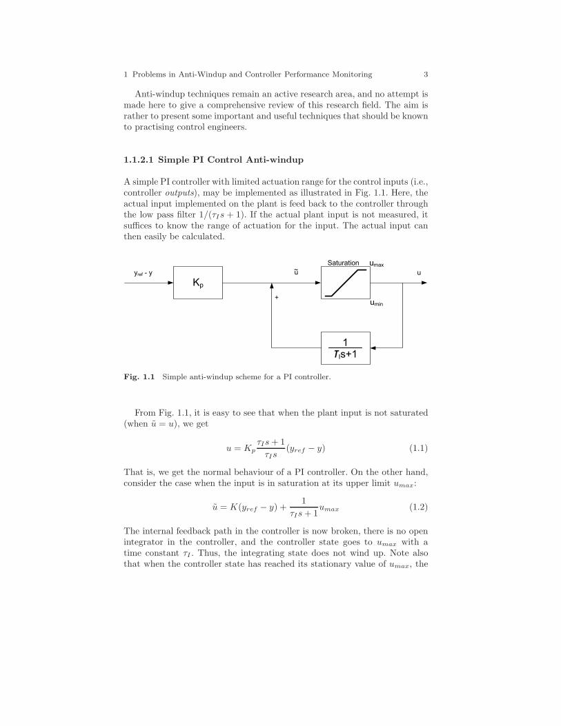
A simple PI controller with limited actuation range for the control inputs (i.e.,controller outputs), may be implemented as illustrated in Fig. 1.1. Here, theactual input implemented on the plant is feed back to the controller throughthe low pass filter 1/(τIs + 1). If the actual plant input is not measured, itsuffices to know the range of actuation for the input. The actual input canthen easily be calculated.
Kp
1τIs+1
umax
umin+
uu~Saturation
yref - y
Fig. 1.1 Simple anti-windup scheme for a PI controller.
From Fig. 1.1, it is easy to see that when the plant input is not saturated(when u = u), we get
u = KpτIs+ 1
τIs(yref − y) (1.1)
That is, we get the normal behaviour of a PI controller. On the other hand,consider the case when the input is in saturation at its upper limit umax:
u = K(yref − y) +1
τIs+ 1umax (1.2)
The internal feedback path in the controller is now broken, there is no openintegrator in the controller, and the controller state goes to umax with atime constant τI . Thus, the integrating state does not wind up. Note alsothat when the controller state has reached its stationary value of umax, the
4 Morten Hovd and Selvanathan Sivalingam
controller output will stay at its maximum value until the measurement yhas crossed the reference value yref .
This anti-windup scheme is straight forward and simple to implement pro-vided any actuator dynamics is fast compared to the PI controller time con-stant τI .
1.1.2.2 Velocity Form of PI Controllers
The PI controller in (1.1) is in position form, i.e., the controller output cor-responds to the desired position/value of the plant input. Alternatively, thecontroller output may give the desired change in the plant input.
Whereas the equations for PI controllers in position form are often ex-pressed in continuous time (even though the final implementation in a plantcomputer will be in discrete time), the velocity form of the PI controller ismost often expressed in discrete time. Let the subscript denote the discretetime index, and ek = yref − yk be the control offset at time k. The discretetime equivalent of (1.1) may then be expressed as
∆uk = uk − uk−1 =T
τIek−1 +Kp(ek − ek−1) (1.3)
where T is the sample interval. Here ∆uk represents the change in the plantinput at time k. If this change is sent to the actuator for the plant input,instead of the desired position of the input, the windup problem goes away.This is because desired changes that violate the actuation constraints simplywill not have any effect. Note that the actuator should implementnew desired value = present value + ∆uk
If the previous desired value is used instead of present value above, the velocityform of the controller will not remove windup problems.
The velocity form can also be found for more complex controllers, in par-ticular for PID controllers. However, derivative action is normally rather fast,and the effects thereof quickly die out. It is therefore often not considerednecessary to account for the derivative action in anti-windup of PID con-trollers.
1.1.2.3 Anti-windup in Cascaded Control Systems
For ordinary plant input, it is usually simple to determine the range of actu-ation. For instance, a valve opening is constrained to be within 0 and 100%,maximum and minimum operating speeds for pumps are often well known,etc. In the case of cascaded control loops, the ’plant input’ seen by the outerloop is actually the reference signal to the inner loop, and the control istypically based on the assumption that the inner loop is able to follow thereference changes set by the outer loop. In such cases, the ’available range of

1 Problems in Anti-Windup and Controller Performance Monitoring 5
actuation’ for the outer loop may be harder to determine, and may dependon operating conditions. An example of this problem may be a temperaturecontrol system, where the temperature control loop is the outer loop, andthe inner loop is a cooling water flow control loop with the valve openingas the plant input. In such an example, the maximum achievable flowratemay depend on up- and downstream pressures, which may depend on coolingwater demand elsewhere in the system.
Possible ways of handling anti-windup of the outer loop in such a situationinclude
• Using conservative estimates of the available range of actuation, with thepossibility of not fully utilising plant capacity in some operating scenaria.
• The controller in the inner loop may send a signal informing the controllerin the outer loop when it is in saturation (and whether it is at its maximumor minimum value). The controller in the outer loop may then stop theintegration if this would move the controller output in the wrong direction.
• Use the velocity form of the controller, provided the reference signal forthe inner loop is calculated as present plant output + change in referencefrom outer loop. If the reference signal is calculated as ’reference at lasttime step + change in reference from outer loop’, windup may still occur.
• For PI controllers, use the implementation shown in Fig. 1.1, where the’plant input’ used in the outer loop is the plant measurement for the innerloop.
Note that the two latter anti-windup schemes above both require a cleartimescale separation between the loops (the inner loop being faster than theouter loop), otherwise performance may suffer when the plant input (in theinner loop) is not in saturation. There is usually a clear timescale separationbetween cascaded loops.
1.1.2.4 Hanus’ Self-conditioned Form
Hanus’ self-conditioned form (Hanus et al (1987); Skogestad and Postleth-waite (2005)) is a quite general way of preventing windup in controllers.Assume a linear controller is used, with state space realization
v = AKv +BKe (1.4)
u = CKv +DKe (1.5)
where v are the controller states, e are the (ordinary) controller inputs, andu is the calculated output from the controller (desired plant input). Thecorresponding controller transfer function may be expressed as
K(s)s=
[AK BK
CK DK
]= CK(sI −AK)−1BK +DK (1.6)
6 Morten Hovd and Selvanathan Sivalingam
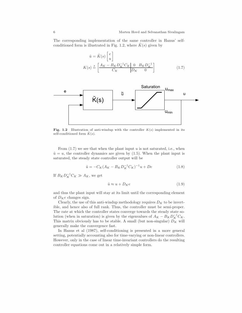
The corresponding implementation of the same controller in Hanus’ self-conditioned form is illustrated in Fig. 1.2, where K(s) given by
u = K(s)
[eu
]
K(s)s=
[AK −BKD−1
K CK 0 BKD−1K
CK DK 0
](1.7)
umax
umin
uu~
Saturation
e
~
Fig. 1.2 Illustration of anti-windup with the controller K(s) implemented in itsself-conditioned form K(s).
From (1.7) we see that when the plant input u is not saturated, i.e., whenu = u, the controller dynamics are given by (1.5). When the plant input issaturated, the steady state controller output will be
u = −CK(AK −BKD−1K CK)−1u+De (1.8)
If BKD−1K CK ≫ AK , we get
u ≈ u+DKe (1.9)
and thus the plant input will stay at its limit until the corresponding elementof DKe changes sign.
Clearly, the use of this anti-windup methodology requiresDK to be invert-ible, and hence also of full rank. Thus, the controller must be semi-proper.The rate at which the controller states converge towards the steady state so-lution (when in saturation) is given by the eigenvalues of AK −BKD−1
K CK .This matrix obviously has to be stable. A small (but non-singular) DK willgenerally make the convergence fast.
In Hanus et al (1987), self-conditioning is presented in a more generalsetting, potentially accounting also for time-varying or non-linear controllers.However, only in the case of linear time-invariant controllers do the resultingcontroller equations come out in a relatively simple form.
1 Problems in Anti-Windup and Controller Performance Monitoring 7
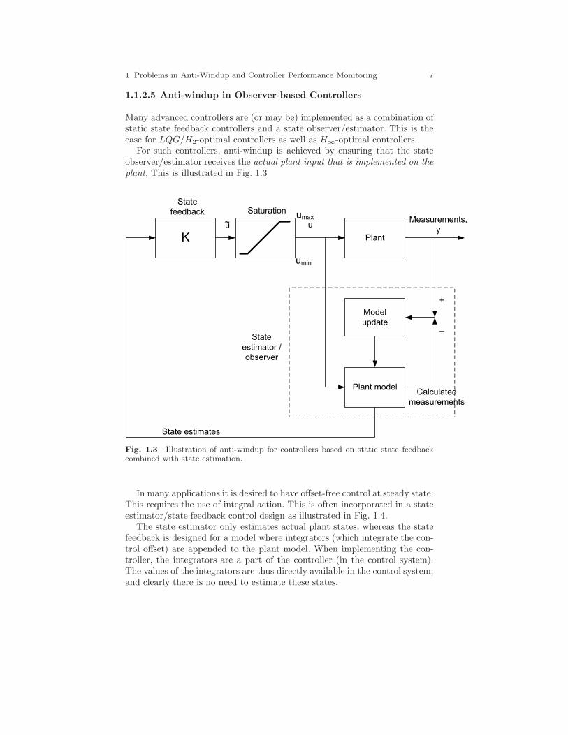
1.1.2.5 Anti-windup in Observer-based Controllers
Many advanced controllers are (or may be) implemented as a combination ofstatic state feedback controllers and a state observer/estimator. This is thecase for LQG/H2-optimal controllers as well as H∞-optimal controllers.
For such controllers, anti-windup is achieved by ensuring that the stateobserver/estimator receives the actual plant input that is implemented on theplant. This is illustrated in Fig. 1.3
uu~
State
feedback umax
umin
Saturation
Plant
Plant model
Measurements,
y
+
_
Model
update
State
estimator /
observer
State estimates
Calculated
measurements
Fig. 1.3 Illustration of anti-windup for controllers based on static state feedbackcombined with state estimation.
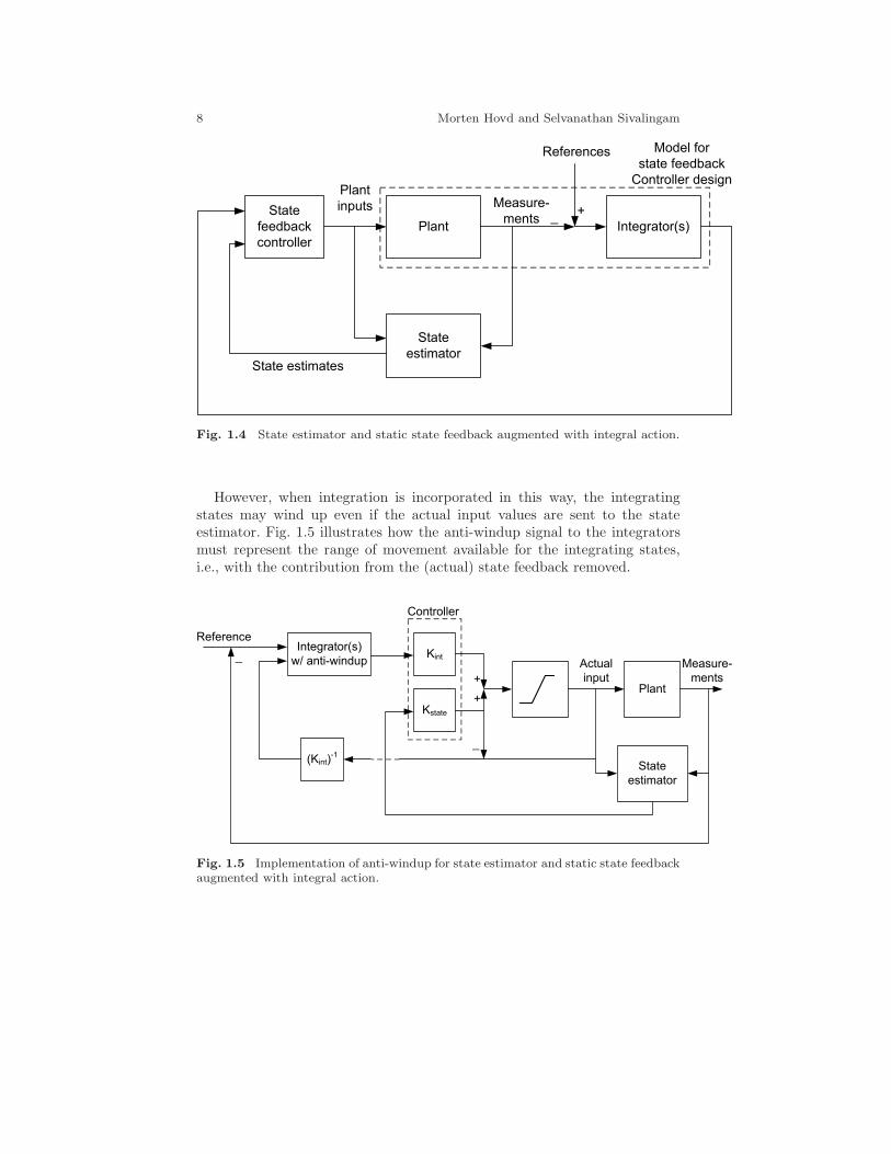
In many applications it is desired to have offset-free control at steady state.This requires the use of integral action. This is often incorporated in a stateestimator/state feedback control design as illustrated in Fig. 1.4.
The state estimator only estimates actual plant states, whereas the statefeedback is designed for a model where integrators (which integrate the con-trol offset) are appended to the plant model. When implementing the con-troller, the integrators are a part of the controller (in the control system).The values of the integrators are thus directly available in the control system,and clearly there is no need to estimate these states.
8 Morten Hovd and Selvanathan Sivalingam
Plant
State
estimator
State
feedback
controller
State estimates
Measure-
ments
Plant
inputs_
+
References
Integrator(s)
Model for
state feedback
Controller design
Fig. 1.4 State estimator and static state feedback augmented with integral action.
However, when integration is incorporated in this way, the integratingstates may wind up even if the actual input values are sent to the stateestimator. Fig. 1.5 illustrates how the anti-windup signal to the integratorsmust represent the range of movement available for the integrating states,i.e., with the contribution from the (actual) state feedback removed.
Plant
Kint
Kstate
+
+
State
estimator
Integrator(s)
w/ anti-windup
Reference
Actual
input
Measure-
ments
_
_
(Kint)-1
Controller
Fig. 1.5 Implementation of anti-windup for state estimator and static state feedbackaugmented with integral action.

1 Problems in Anti-Windup and Controller Performance Monitoring 9
Remark. Note that if Hanus’ self-conditioned form is used for the anti-windup, this requires a non-singularD-matrix, resulting in a PI block insteadof a purely integrating block. The size of this D-matrix may affect controllerperformance (depending on how and whether it is accounted for in the ’state’feedback control design).
1.1.3 Decoupling and Input Constraints
Decouplers are particularly prone to performance problems due to input con-straints. This is not easily handled by standard anti-windup, because much ofthe input usage can be related to counteracting interactions. Therefore, if anoutput is saturated, but other outputs are adjusted to counteract the effectsof the ’unsaturated’ output, severe performance problems may be expected.
One way of ensuring that the decoupler only tries to counteract interactionsdue to the inputs that are actually implemented on the plant, is to implementthe decoupler as illustrated in Fig. 1.6.
2
1
12
11
21
22
Controller,
loop 1
Controller,
loop 2
Unsaturated
inputs
r1
r2
_
_
Saturated
inputs
Plant
y1
y2
Fig. 1.6 Implementation of decoupler in order to reduce the effect of input satura-tion. The decoupler will only attempt to counteract interactions due to inputs thatare actually implemented on the plant.
The implementation in Fig. 1.6 is easily extended to systems of dimensionhigher than 2 × 2. When the inputs are unsaturated, the ’Decoupler withsaturation’ in Fig. 1.1 corresponds to the decoupling compensator W (s) =G(s)−1G(s), where G(s) denotes the diagonal matrix with the same diagonal
10 Morten Hovd and Selvanathan Sivalingam
elements as G(s). The precompensated plant therefore becomes GW = G,i.e., we are (nominally) left only with the diagonal elements of the plant.
Note that if the individual loop controllers ki(s) contain slow dynamics(which is usually the case, PI controllers are often used), they will still needanti-windup. In this case the anti-windup signal to the controller should notbe the saturated input, but the saturated input with the contribution from thedecoupling removed, i.e., the decoupling means that the saturation limitationsfor the individual loop controllers ki(s) are time variant.
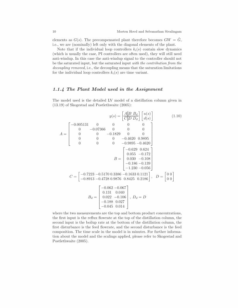
1.1.4 The Plant Model used in the Assignment
The model used is the detailed LV model of a distillation column given in(13.19) of Skogestad and Postlethwaite (2005):
y(s) =
[A B Bd
C D Dd
] [u(s)d(s)
](1.10)
A =
−0.005131 0 0 0 00 −0.07366 0 0 00 0 −0.1829 0 00 0 0 −0.4620 0.98950 0 0 −0.9895 −0.4620
B =
−0.629 0.6240.055 −0.1720.030 −0.108−0.186 −0.139−1.230 −0.056
C =
[−0.7223 −0.5170 0.3386 −0.1633 0.1121−0.8913 −0.4728 0.9876 0.8425 0.2186
], D =
[0 00 0
]
Bd =
−0.062 −0.0670.131 0.0400.022 −0.106−0.188 0.027−0.045 0.014
, Dd = D
where the two measurements are the top and bottom product concentrations,the first input is the reflux flowrate at the top of the distillation column, thesecond input is the boilup rate at the bottom of the distillation column, thefirst disturbance is the feed flowrate, and the second disturbance is the feedcomposition. The time scale in the model is in minutes. For further informa-tion about the model and the scalings applied, please refer to Skogestad andPostlethwaite (2005).
1 Problems in Anti-Windup and Controller Performance Monitoring 11
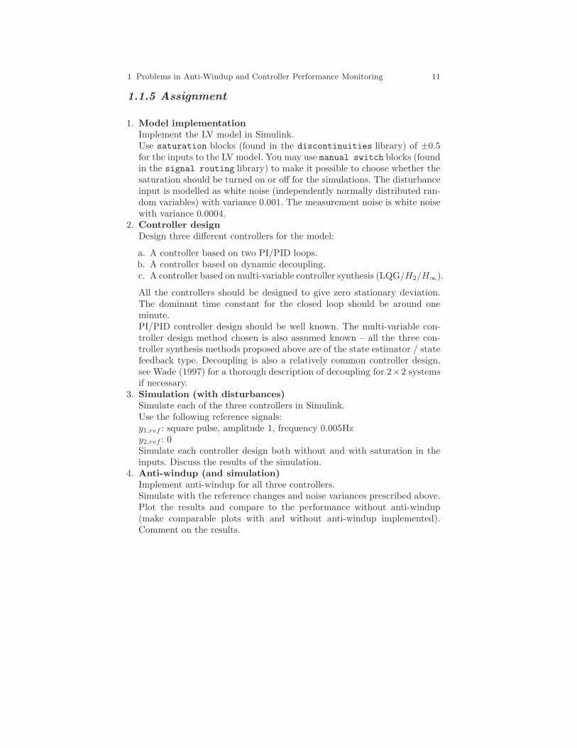
1.1.5 Assignment
1. Model implementationImplement the LV model in Simulink.Use saturation blocks (found in the discontinuities library) of ±0.5for the inputs to the LV model. You may use manual switch blocks (foundin the signal routing library) to make it possible to choose whether thesaturation should be turned on or off for the simulations. The disturbanceinput is modelled as white noise (independently normally distributed ran-dom variables) with variance 0.001. The measurement noise is white noisewith variance 0.0004.
2. Controller designDesign three different controllers for the model:
a. A controller based on two PI/PID loops.b. A controller based on dynamic decoupling.c. A controller based on multi-variable controller synthesis (LQG/H2/H∞).
All the controllers should be designed to give zero stationary deviation.The dominant time constant for the closed loop should be around oneminute.PI/PID controller design should be well known. The multi-variable con-troller design method chosen is also assumed known – all the three con-troller synthesis methods proposed above are of the state estimator / statefeedback type. Decoupling is also a relatively common controller design,see Wade (1997) for a thorough description of decoupling for 2×2 systemsif necessary.
3. Simulation (with disturbances)Simulate each of the three controllers in Simulink.Use the following reference signals:y1,ref : square pulse, amplitude 1, frequency 0.005Hzy2,ref : 0Simulate each controller design both without and with saturation in theinputs. Discuss the results of the simulation.
4. Anti-windup (and simulation)Implement anti-windup for all three controllers.Simulate with the reference changes and noise variances prescribed above.Plot the results and compare to the performance without anti-windup(make comparable plots with and without anti-windup implemented).Comment on the results.
12 Morten Hovd and Selvanathan Sivalingam
1.1.6 Solution
1.1.6.1 Model Implementation
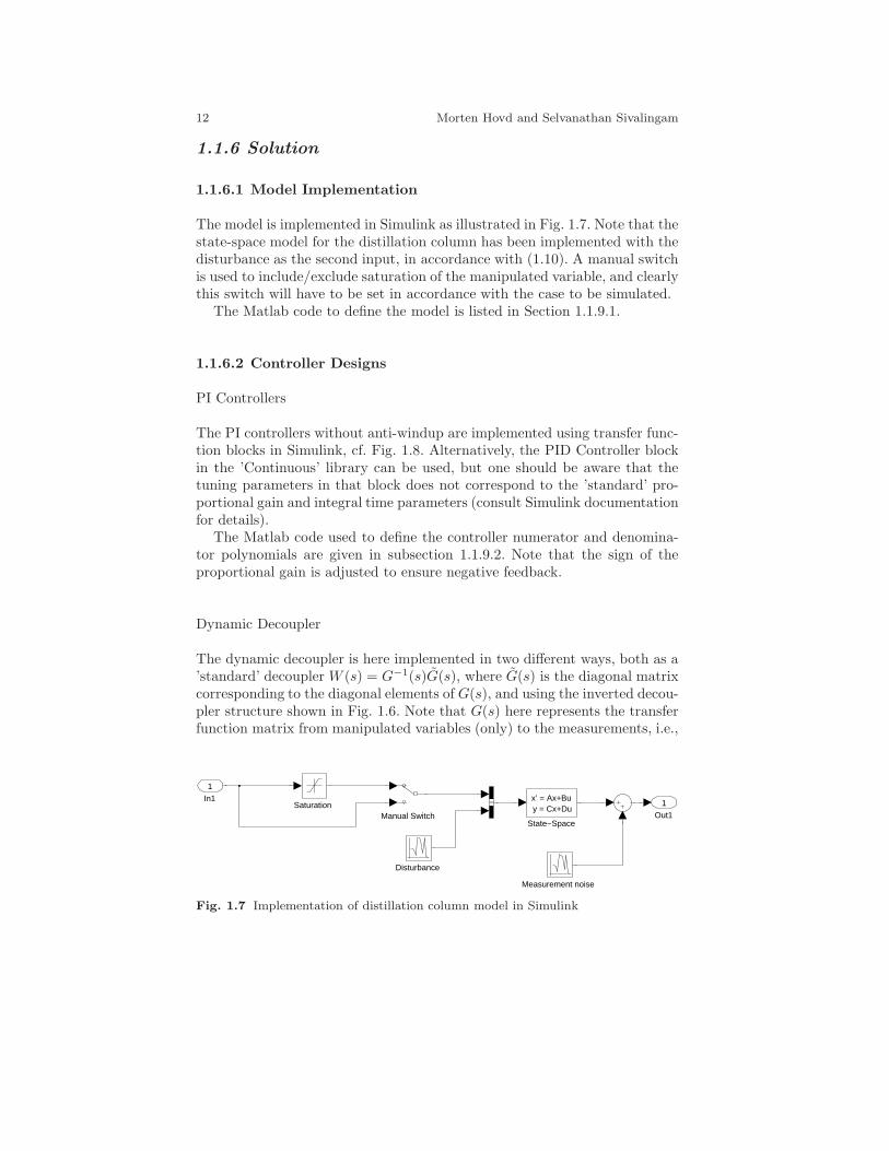
The model is implemented in Simulink as illustrated in Fig. 1.7. Note that thestate-space model for the distillation column has been implemented with thedisturbance as the second input, in accordance with (1.10). A manual switchis used to include/exclude saturation of the manipulated variable, and clearlythis switch will have to be set in accordance with the case to be simulated.
The Matlab code to define the model is listed in Section 1.1.9.1.
1.1.6.2 Controller Designs
PI Controllers
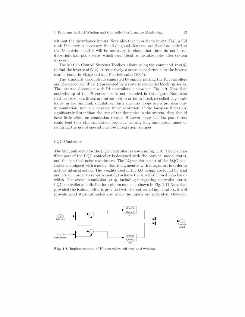
The PI controllers without anti-windup are implemented using transfer func-tion blocks in Simulink, cf. Fig. 1.8. Alternatively, the PID Controller blockin the ’Continuous’ library can be used, but one should be aware that thetuning parameters in that block does not correspond to the ’standard’ pro-portional gain and integral time parameters (consult Simulink documentationfor details).
The Matlab code used to define the controller numerator and denomina-tor polynomials are given in subsection 1.1.9.2. Note that the sign of theproportional gain is adjusted to ensure negative feedback.
Dynamic Decoupler
The dynamic decoupler is here implemented in two different ways, both as a’standard’ decoupler W (s) = G−1(s)G(s), where G(s) is the diagonal matrixcorresponding to the diagonal elements of G(s), and using the inverted decou-pler structure shown in Fig. 1.6. Note that G(s) here represents the transferfunction matrix from manipulated variables (only) to the measurements, i.e.,
Out1
1
State−Space
x’ = Ax+Bu y = Cx+DuSaturation
Measurement noise
Manual Switch
Disturbance
In1
1
Fig. 1.7 Implementation of distillation column model in Simulink
1 Problems in Anti-Windup and Controller Performance Monitoring 13
without the disturbance inputs. Note also that in order to invert G(s), a fullrank D matrix is necessary. Small diagonal elements are therefore added tothe D matrix – and it will be necessary to check that these do not intro-duce right half plane zeros, which would lead to unstable poles after systeminversion.
The Matlab Control Systems Toolbox allows using the command inv(G)
to find the inverse of G(s). Alternatively, a state space formula for the inversecan be found in Skogestad and Postlethwaite (2005).
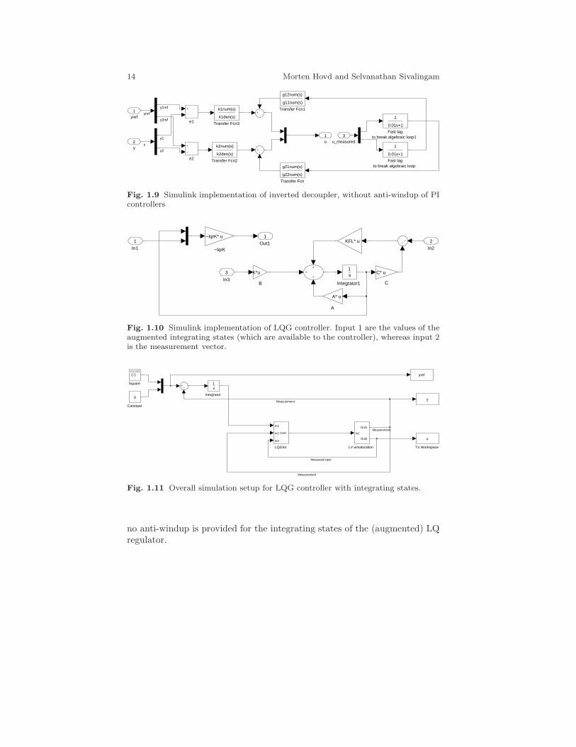
The ’standard’ decoupler is simulated by simply putting the PI controllersand the decoupler W (s) (represented by a state space model block) in series.The inverted decoupler with PI controllers is shown in Fig. 1.9. Note thatanti-windup of the PI controllers is not included in this figure. Note alsothat fast low-pass filters are introduced in order to break so-called ’algebraicloops’ in the Simulink simulation. Such algebraic loops are a problem onlyin simulation, not in a physical implementation. If the low-pass filters aresignificantly faster than the rest of the dynamics in the system, they shouldhave little effect on simulation results. However, very fast low-pass filterscould lead to a stiff simulation problem, causing long simulation times orrequiring the use of special purpose integration routines.
LQG Controller
The Simulink setup for the LQG controller is shown in Fig. 1.10. The Kalmanfilter part of the LQG controller is designed with the physical model states,and the specified noise covariances. The LQ regulator part of the LQG con-troller is designed with a model that is augmented with integrators in order toinclude integral action. The weights used in the LQ design are found by trialand error in order to (approximately) achieve the specified closed loop band-width. The overall simulation setup, including integrating controller states,LQG controller and distillation column model, is shown in Fig. 1.11 Note thatprovided the Kalman filter is provided with the saturated input values, it willprovide good state estimates also when the inputs are saturated. However,
Controlleroutput
1
PI2
k2num(s)
k2den(s)
PI1
k1num(s)
k1den(s)
Measurement
2
Reference
1
Fig. 1.8 Implementation of PI controllers without anti-windup.
14 Morten Hovd and Selvanathan Sivalingam
u1
e2
e1 Transfer Fcn3
k1num(s)
k1den(s)
Transfer Fcn2
k2num(s)
k2den(s)
Transfer Fcn1
g12num(s)
g11num(s)
Transfer Fcn
g21num(s)
g22num(s)
Fast lagto break algebraic loop1
1
0.01s+1
Fast lagto break algebraic loop
1
0.01s+1
u_measured3
y2
yref1
y
yref
y1ref
y1
y2ref
y2
Fig. 1.9 Simulink implementation of inverted decoupler, without anti-windup of PIcontrollers
Out1
1
Integrator1
1s
C
C* u
B
K*u
A
A* u
−lqrK
−lqrK* uKFL* u
In3
3
In2
2
In1
1
Fig. 1.10 Simulink implementation of LQG controller. Input 1 are the values of theaugmented integrating states (which are available to the controller), whereas input 2is the measurement vector.
To Workspace
u
Square
LV w/saturation
In1
Out1
Out2
LQGint
In1
In2
In3
Out1
Integrator
1s
Constant
0 y
yref
Measurement
Measurement
Measurement
Measured input
Fig. 1.11 Overall simulation setup for LQG controller with integrating states.
no anti-windup is provided for the integrating states of the (augmented) LQregulator.
1 Problems in Anti-Windup and Controller Performance Monitoring 15
1.1.7 Simulations
1.1.7.1 PI Controller
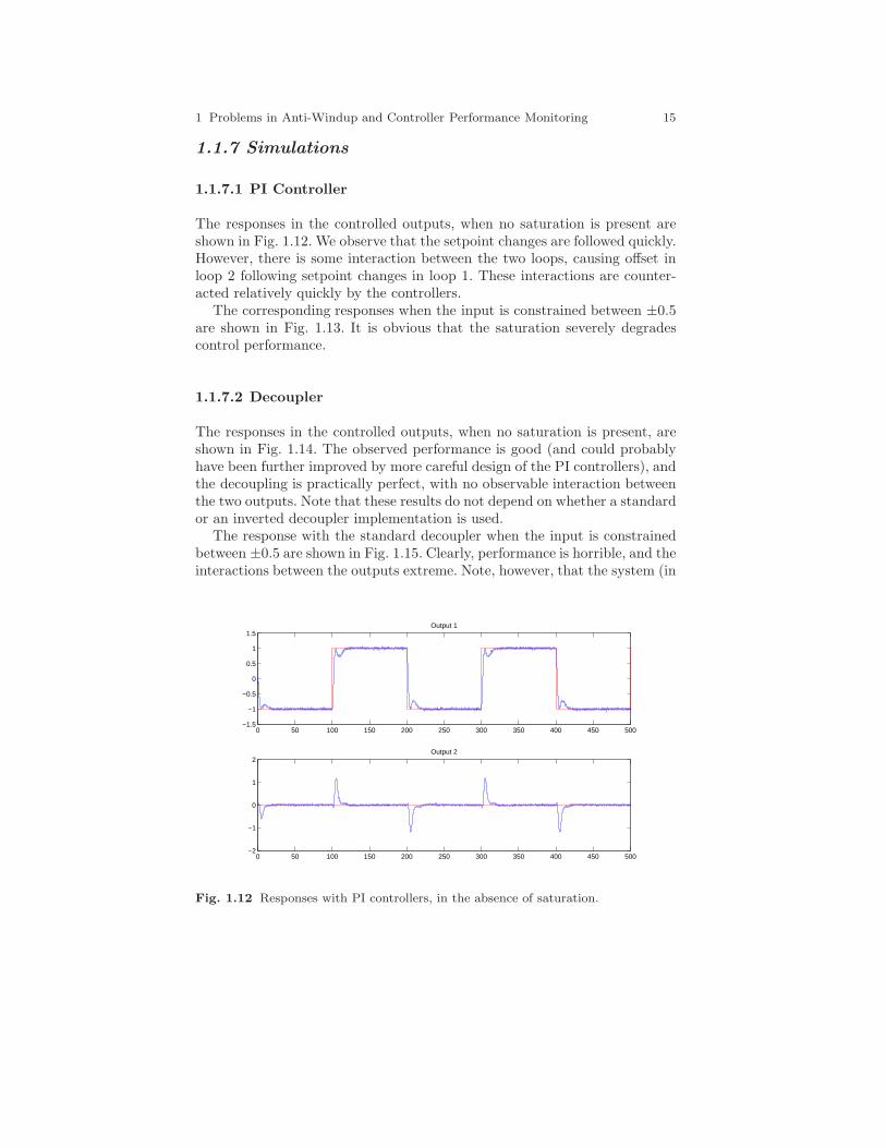
The responses in the controlled outputs, when no saturation is present areshown in Fig. 1.12. We observe that the setpoint changes are followed quickly.However, there is some interaction between the two loops, causing offset inloop 2 following setpoint changes in loop 1. These interactions are counter-acted relatively quickly by the controllers.
The corresponding responses when the input is constrained between ±0.5are shown in Fig. 1.13. It is obvious that the saturation severely degradescontrol performance.
1.1.7.2 Decoupler
The responses in the controlled outputs, when no saturation is present, areshown in Fig. 1.14. The observed performance is good (and could probablyhave been further improved by more careful design of the PI controllers), andthe decoupling is practically perfect, with no observable interaction betweenthe two outputs. Note that these results do not depend on whether a standardor an inverted decoupler implementation is used.
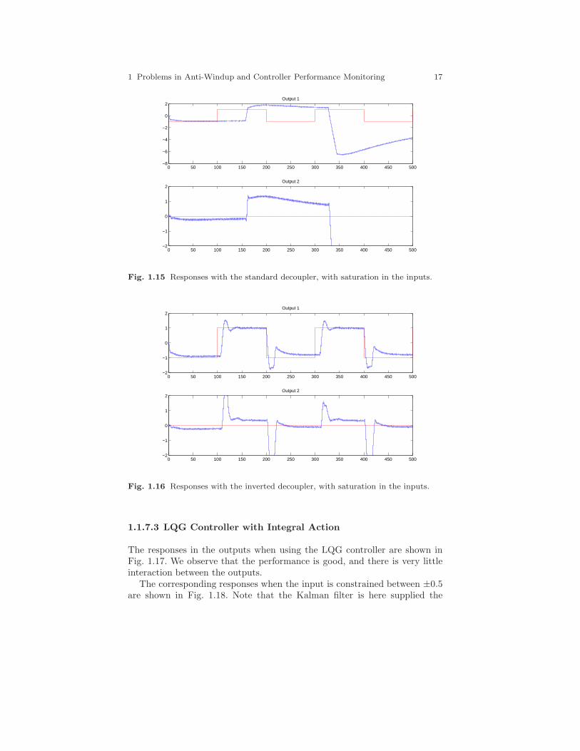
The response with the standard decoupler when the input is constrainedbetween ±0.5 are shown in Fig. 1.15. Clearly, performance is horrible, and theinteractions between the outputs extreme. Note, however, that the system (in
0 50 100 150 200 250 300 350 400 450 500−1.5
−1
−0.5
0
0.5
1
1.5Output 1
0 50 100 150 200 250 300 350 400 450 500−2
−1
0
1
2Output 2
Fig. 1.12 Responses with PI controllers, in the absence of saturation.

16 Morten Hovd and Selvanathan Sivalingam
0 50 100 150 200 250 300 350 400 450 500−2
−1
0
1
2Output 1
0 50 100 150 200 250 300 350 400 450 500−2
−1
0
1
2Output 2
Fig. 1.13 Responses with PI controllers, with saturation in the inputs.
0 50 100 150 200 250 300 350 400 450 500−2
−1
0
1
2Output 1
0 50 100 150 200 250 300 350 400 450 500−2
−1
0
1
2Output 2
Fig. 1.14 Responses with decoupler, in the absence of saturation.
this case) remains stable – although the responses leave the window displayedin the figure.
The corresponding response with the inverted decoupler are shown inFig. 1.16. We see that the performance is much better than with the stan-dard decoupler, although there is still significant interactions between theoutputs. These responses still suffer from the absence of anti-windup for thePI controllers used for the individual loops.
1 Problems in Anti-Windup and Controller Performance Monitoring 17
0 50 100 150 200 250 300 350 400 450 500−8
−6
−4
−2
0
2Output 1
0 50 100 150 200 250 300 350 400 450 500−2
−1
0
1
2Output 2
Fig. 1.15 Responses with the standard decoupler, with saturation in the inputs.
0 50 100 150 200 250 300 350 400 450 500−2
−1
0
1
2Output 1
0 50 100 150 200 250 300 350 400 450 500−2
−1
0
1
2Output 2
Fig. 1.16 Responses with the inverted decoupler, with saturation in the inputs.
1.1.7.3 LQG Controller with Integral Action
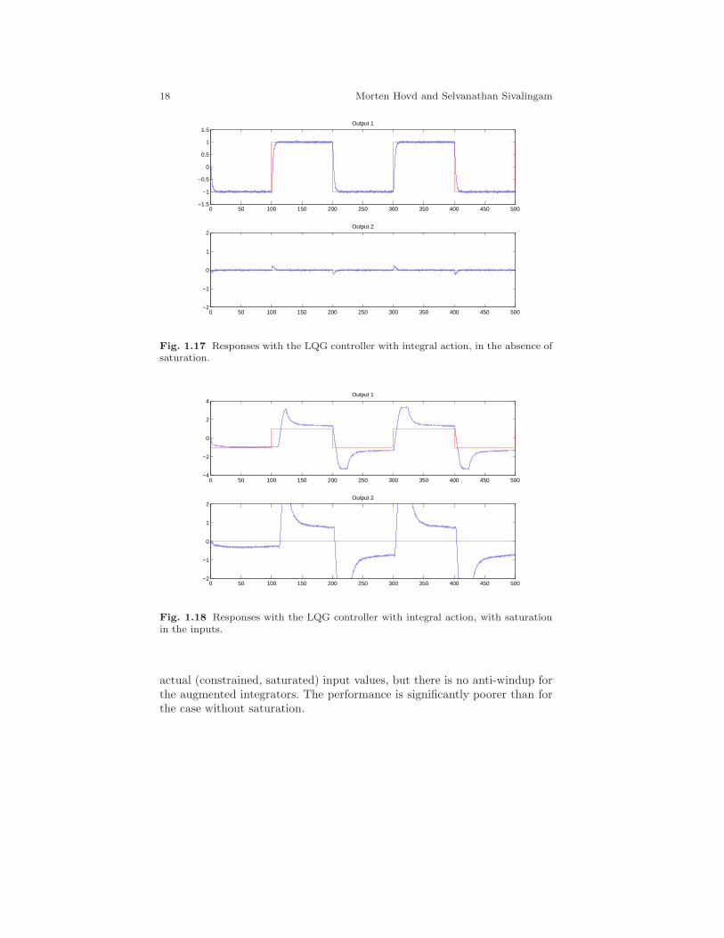
The responses in the outputs when using the LQG controller are shown inFig. 1.17. We observe that the performance is good, and there is very littleinteraction between the outputs.
The corresponding responses when the input is constrained between ±0.5are shown in Fig. 1.18. Note that the Kalman filter is here supplied the
18 Morten Hovd and Selvanathan Sivalingam
0 50 100 150 200 250 300 350 400 450 500−1.5
−1
−0.5
0
0.5
1
1.5Output 1
0 50 100 150 200 250 300 350 400 450 500−2
−1
0
1
2Output 2
Fig. 1.17 Responses with the LQG controller with integral action, in the absence ofsaturation.
0 50 100 150 200 250 300 350 400 450 500−4
−2
0
2
4Output 1
0 50 100 150 200 250 300 350 400 450 500−2
−1
0
1
2Output 2
Fig. 1.18 Responses with the LQG controller with integral action, with saturationin the inputs.
actual (constrained, saturated) input values, but there is no anti-windup forthe augmented integrators. The performance is significantly poorer than forthe case without saturation.
1 Problems in Anti-Windup and Controller Performance Monitoring 19
Out1
1
Transfer Fcn1
1
Ti2.s+1
Transfer Fcn
1
Ti1.s+1
Gain1
Kp2
Gain
Kp1
In3
3
In2
2
In1
1
Fig. 1.19 Implementation of two PI controllers with simple anti-windup techniquein Simulink.
1.1.7.4 Conclusion on Simulation Results
The simulations show that all three controller types are able to achieve goodcontrol of the plant. For all three controllers, the performance is significantlydegraded in the presence of saturation, although to different degrees for thedifferent controllers.
1.1.8 Anti-windup
In this section, anti-windup is implemented for all three controllers, and thesimulations re-run.
1.1.8.1 PI Controllers
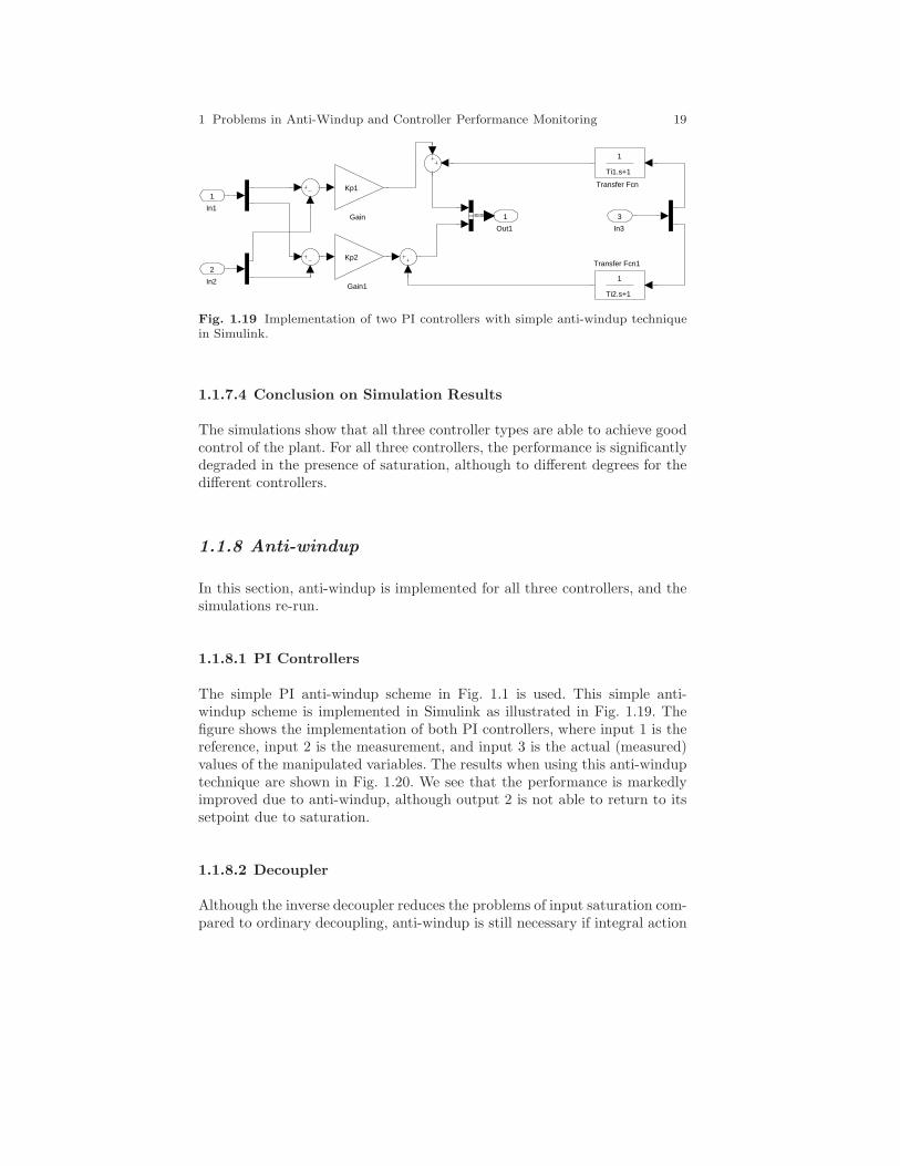
The simple PI anti-windup scheme in Fig. 1.1 is used. This simple anti-windup scheme is implemented in Simulink as illustrated in Fig. 1.19. Thefigure shows the implementation of both PI controllers, where input 1 is thereference, input 2 is the measurement, and input 3 is the actual (measured)values of the manipulated variables. The results when using this anti-winduptechnique are shown in Fig. 1.20. We see that the performance is markedlyimproved due to anti-windup, although output 2 is not able to return to itssetpoint due to saturation.
1.1.8.2 Decoupler
Although the inverse decoupler reduces the problems of input saturation com-pared to ordinary decoupling, anti-windup is still necessary if integral action

20 Morten Hovd and Selvanathan Sivalingam
0 50 100 150 200 250 300 350 400 450 500−1.5
−1
−0.5
0
0.5
1
1.5Output 1
0 50 100 150 200 250 300 350 400 450 500−2
−1
0
1
2Output 2
Fig. 1.20 Response with PI controllers with anti-windup.
u1
k2(Hanus)
x’ = Ax+Bu y = Cx+Du
k1(Hanus)
x’ = Ax+Bu y = Cx+Du
e2
e1
Transfer Fcn1
g12num(s)
g11num(s)
Transfer Fcn
g21num(s)
g22num(s)
Fast lagto break algebraic loop1
1
0.01s+1
Fast lagto break algebraic loop
1
0.01s+1
u_measured3
y2
yref1
y
yref
y1ref
y1
y2ref
y2
Fig. 1.21 Simulink implementation of inverse decoupler with anti-windup for outerPI controllers.
is used in the controllers for the individual loops that result after decouplingcompensation. This is the common case, which also is used in this example.However, even if simple PI controllers are used in the individual loops, wemay can no longer use the simple anti-windup scheme in Fig. 1.1. Rather, wehave to calculate the range of manipulated (input) variable movement that isavailable, after accounting for the action of the decoupling elements. This isis illustrated by the Simulink implementation in Fig. 1.21. Note that here theanti-windup of the PI controllers has been achieved using the so-called Hanusform. This could equivalently have been done using the scheme in Fig. 1.1.
The resulting responses when using the inverted decoupler with anti-windup are shown in Fig. 1.22. Comparing to Fig. 1.16, we see that the
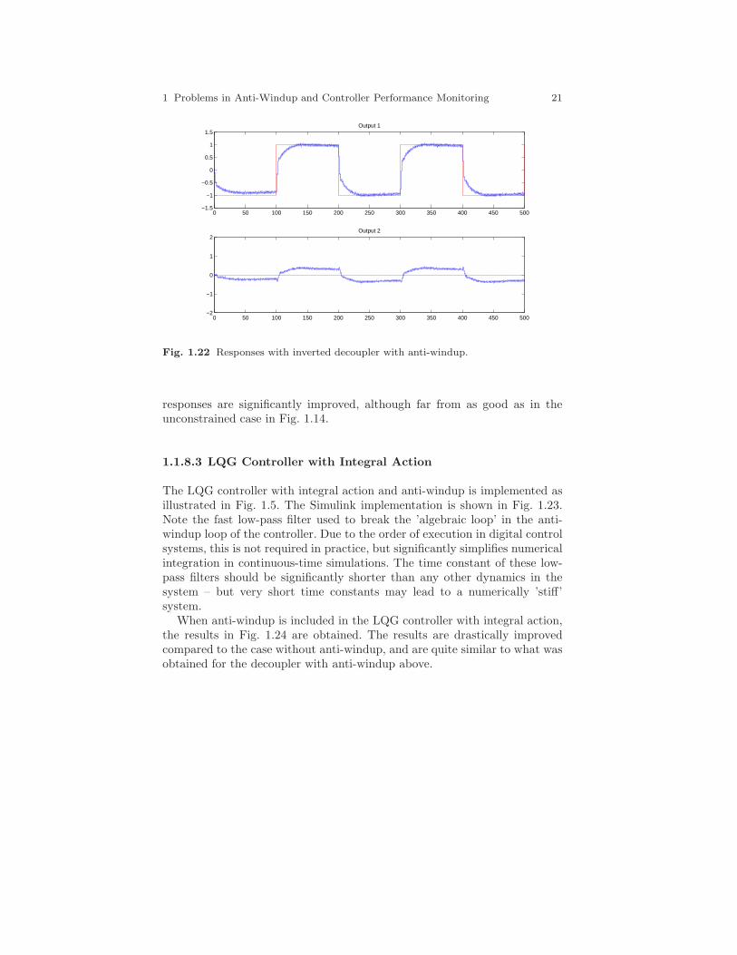
1 Problems in Anti-Windup and Controller Performance Monitoring 21
0 50 100 150 200 250 300 350 400 450 500−1.5
−1
−0.5
0
0.5
1
1.5Output 1
0 50 100 150 200 250 300 350 400 450 500−2
−1
0
1
2Output 2
Fig. 1.22 Responses with inverted decoupler with anti-windup.
responses are significantly improved, although far from as good as in theunconstrained case in Fig. 1.14.
1.1.8.3 LQG Controller with Integral Action
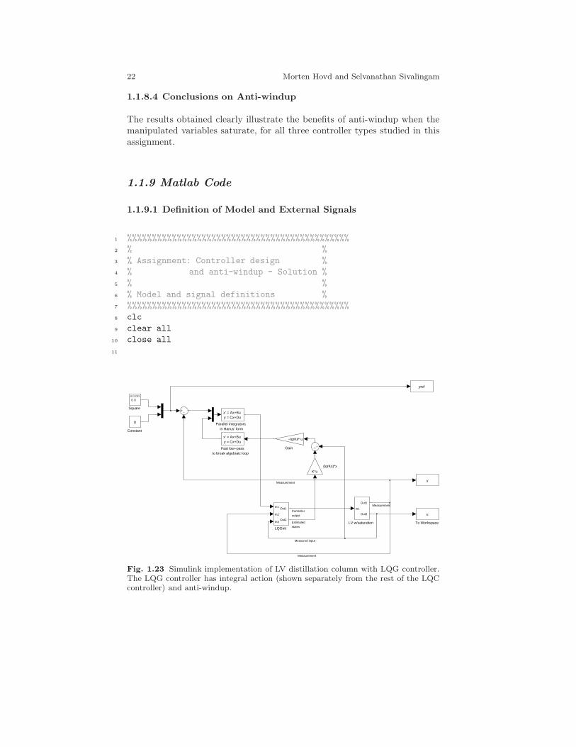
The LQG controller with integral action and anti-windup is implemented asillustrated in Fig. 1.5. The Simulink implementation is shown in Fig. 1.23.Note the fast low-pass filter used to break the ’algebraic loop’ in the anti-windup loop of the controller. Due to the order of execution in digital controlsystems, this is not required in practice, but significantly simplifies numericalintegration in continuous-time simulations. The time constant of these low-pass filters should be significantly shorter than any other dynamics in thesystem – but very short time constants may lead to a numerically ’stiff’system.
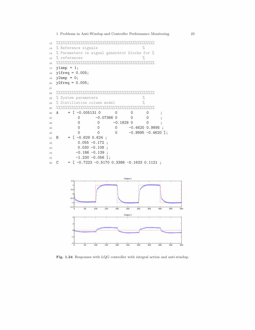
When anti-windup is included in the LQG controller with integral action,the results in Fig. 1.24 are obtained. The results are drastically improvedcompared to the case without anti-windup, and are quite similar to what wasobtained for the decoupler with anti-windup above.
22 Morten Hovd and Selvanathan Sivalingam
1.1.8.4 Conclusions on Anti-windup
The results obtained clearly illustrate the benefits of anti-windup when themanipulated variables saturate, for all three controller types studied in thisassignment.
1.1.9 Matlab Code
1.1.9.1 Definition of Model and External Signals
1 %%%%%%%%%%%%%%%%%%%%%%%%%%%%%%%%%%%%%%%%%%%%%
2 % %
3 % Assignment: Controller design %
4 % and anti-windup - Solution %
5 % %
6 % Model and signal definitions %
7 %%%%%%%%%%%%%%%%%%%%%%%%%%%%%%%%%%%%%%%%%%%%%
8 clc
9 clear all
10 close all
11
To Workspace
u
Square
Parallel integratorsin Hanus’ form
x’ = Ax+Bu y = Cx+Du
LV w/saturation
In1
Out1
Out2
LQGint
In1
In2
In3
Out1
Out2
Gain
−lqrKii* u
Fast low−passto break algebraic loop
x’ = Ax+Bu y = Cx+Du
Constant
0
(lqrKs)*x
K*u
y
yref
Measurement
Measurement
Measurement
Controller
output
Measured input
Estimated
states
Fig. 1.23 Simulink implementation of LV distillation column with LQG controller.The LQG controller has integral action (shown separately from the rest of the LQCcontroller) and anti-windup.
1 Problems in Anti-Windup and Controller Performance Monitoring 23
12 %%%%%%%%%%%%%%%%%%%%%%%%%%%%%%%%%%%%%%%%%%%%%
13 % Reference signals %
14 % Parameters in signal generator blocks for %
15 % references %
16 %%%%%%%%%%%%%%%%%%%%%%%%%%%%%%%%%%%%%%%%%%%%%
17 y1amp = 1;
18 y1freq = 0.005;
19 y2amp = 0;
20 y2freq = 0.005;
21
22 %%%%%%%%%%%%%%%%%%%%%%%%%%%%%%%%%%%%%%%%%%%%%
23 % System parameters %
24 % Distillation column model %
25 %%%%%%%%%%%%%%%%%%%%%%%%%%%%%%%%%%%%%%%%%%%%%
26 A = [ -0.005131 0 0 0 0 ;
27 0 -0.07366 0 0 0 ;
28 0 0 -0.1829 0 0 ;
29 0 0 0 -0.4620 0.9895 ;
30 0 0 0 -0.9895 -0.4620 ];
31 B = [ -0.629 0.624 ;
32 0.055 -0.172 ;
33 0.030 -0.108 ;
34 -0.186 -0.139 ;
35 -1.230 -0.056 ];
36 C = [ -0.7223 -0.5170 0.3386 -0.1633 0.1121 ;
0 50 100 150 200 250 300 350 400 450 500−1.5
−1
−0.5
0
0.5
1
1.5Output 1
0 50 100 150 200 250 300 350 400 450 500−2
−1
0
1
2Output 2
Fig. 1.24 Responses with LQG controller with integral action and anti-windup.

24 Morten Hovd and Selvanathan Sivalingam
37 -0.8913 -0.4728 0.9876 0.8425 0.2186 ];
38 Bd = [ -0.062 -0.067 ;
39 0.131 0.040 ;
40 0.022 -0.106 ;
41 -0.188 0.027 ;
42 -0.045 0.014 ];
43 D = [ 0 0 ;
44 0 0 ];
45 sys = ss(A,B,C,D);
46 G = tf(sys); % Used in decoupler
47
48 %%%%%%%%%%%%%%%%%%%%%%%%%%%%%%%%%%%%%%%%%%%%%
49 % White noise disturbances %
50 % and measurement noise %
51 %%%%%%%%%%%%%%%%%%%%%%%%%%%%%%%%%%%%%%%%%%%%%
52 kw = 0.001;
53 Wvar = kw*ones(2,1); %Disturbance variance
54 QXU = eye(7);
55 kv = 0.0004;
56 Vvar = kv*ones(2,1); %Measurementn noise variance
1.1.9.2 Simple PI Controller without Anti-windup
1 %%%%%%%%%%%%%%%%%%%%%%%%%%%%%%%%%%%%%%%%%%%%%
2 % PI controller %
3 %%%%%%%%%%%%%%%%%%%%%%%%%%%%%%%%%%%%%%%%%%%%%
4 s = tf(’s’);
5 Kp1 = 0.5; Kp2 = -0.5; % Signs are decided through
6 % dcgain(A,B,C,D), which results in
7 % [88.3573 -86.8074; 108.0808 -107.9375]
8 Ti1 = 2; Ti2 = 2;
9 k1 = Kp1*(Ti1*s+1)/(Ti1*s); [k1num,k1den] = tfdata(k1); k1num
= k1num1,:; k1den = k1den1,:;
10 k2 = Kp2*(Ti2*s+1)/(Ti2*s); [k2num,k2den] = tfdata(k2); k2num
= k2num1,:; k2den = k2den1,:;
1.1.9.3 Decoupling
1 % Transfer function matrix G(s) defined in file model.m,
2 % which must be run before this file.
1 Problems in Anti-Windup and Controller Performance Monitoring 25
3 % Similarly, the individual PI controllers used with the
decouplers are
4 % (in this case) identical to the controllers used for (
ordinary) PI control. The file
5 % PIcont.m should therefore also run before this file
6
7 %%%%%%%%%%%%%%%%%%%%%%%%%%%%%%%%%%%%%%%%%%%%%
8 % Dynamic decoupling controller %
9 %%%%%%%%%%%%%%%%%%%%%%%%%%%%%%%%%%%%%%%%%%%%%
10 Gdiag = [G(1,1) 0 ;
11 0 G(2,2) ];
12 % We need a non-singular D-matrix to calculate inv(G).
13 % Find an approximate G using a new D-matrix that does not
14 % introduce poles in the right-half plane
15 dd = [ 1e-3 0 ;
16 0 -1e-3 ];
17 Gapp = ss(A,B,C,dd);
18 %tzero(Gapp) % Check for zeros..
19 W = inv(Gapp)*Gdiag;
20 W = minreal(W);
21 [Wa,Wb,Wc,Wd] = ssdata(W);
22
23 %%%%%%%%%%%%%%%%%%%%%%%%%%%%%%%%%%%%%%%%%%%%%
24 % Anti-windup for dynamic decoupling %
25 %%%%%%%%%%%%%%%%%%%%%%%%%%%%%%%%%%%%%%%%%%%%%
26 % Note that all elements share the same denominator
27 [g11num,g11den] = tfdata(sys(1,1));
28 g11den = g11den1,:; g11num = g11num1,:;
29 [g12num,g12den] = tfdata(sys(1,2));
30 g12den = g12den1,:; g12num = g12num1,:;
31 [g21num,g21den] = tfdata(sys(2,1));
32 g21den = g21den1,:; g21num = g21num1,:;
33 [g22num,g22den] = tfdata(sys(2,2));
34 g22den = g22den1,:; g22num = g22num1,:;
35
36 % Using Hanus’ self-conditioned form for anti-windup
37 % of PI controllers
38 [k2a,k2b,k2c,k2d]=ssdata(k2);
39 [k1a,k1b,k1c,k1d]=ssdata(k1);
40
41 k1aw = k1a-k1b*inv(k1d)*k1c;
42 k1bw = [zeros(size(k1b)) k1b*inv(k1d)];
43 uz = size(k1b*inv(k1d));
44 k1cw = k1c;
45 k1dw = [k1d zeros(uz)];
26 Morten Hovd and Selvanathan Sivalingam
46
47 k2aw = k2a-k2b*inv(k2d)*k2c;
48 k2bw = [zeros(size(k2b)) k2b*inv(k2d)];
49 uz = size(k2b*inv(k2d));
50 k2cw = k2c;
51 k2dw = [k2d zeros(uz)];
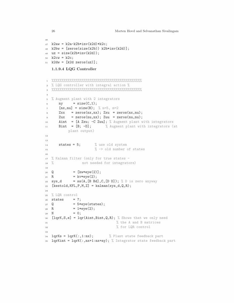
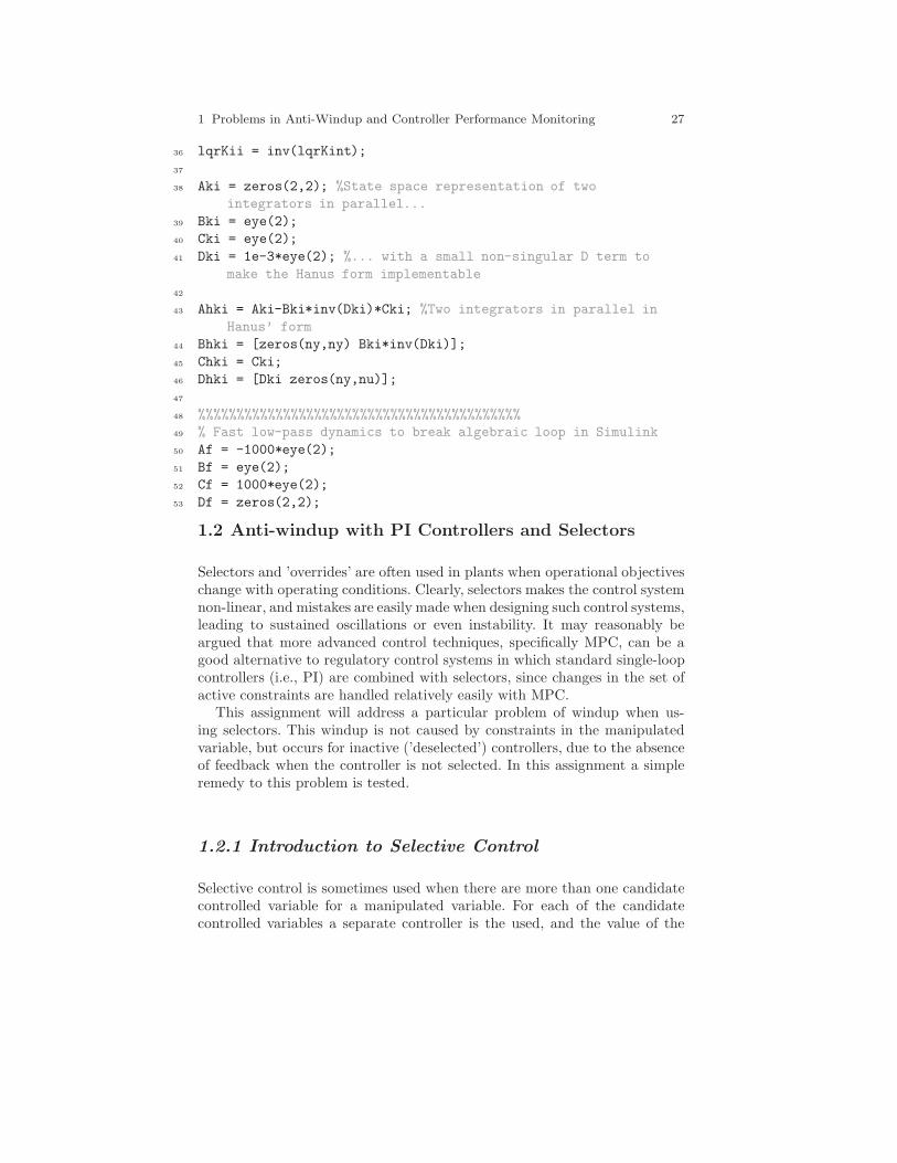
1.1.9.4 LQG Controller
1 %%%%%%%%%%%%%%%%%%%%%%%%%%%%%%%%%%%%%%%%%%%%%
2 % LQG controller with integral action %
3 %%%%%%%%%%%%%%%%%%%%%%%%%%%%%%%%%%%%%%%%%%%%%
4
5 % Augment plant with 2 integrators
6 ny = size(C,1);
7 [nx,nu] = size(B); % n=5, m=2
8 Zxx = zeros(nx,nx); Zxu = zeros(nx,nu);
9 Zux = zeros(nu,nx); Zuu = zeros(nu,nu);
10 Aint = [A Zxu; -C Zuu]; % Augment plant with integrators
11 Bint = [B; -D]; % Augment plant with integrators (at
plant output)
12
13
14 states = 5; % use old system
15 % -> old number of states
16
17 % Kalman filter (only for true states -
18 % not needed for integrators)
19
20 Q = [kw*eye(2)];
21 R = kv*eye(2);
22 sys_d = ss(A,[B Bd],C,[D D]); % D is zero anyway
23 [kestold,KFL,P,M,Z] = kalman(sys_d,Q,R);
24
25 % LQR control
26 states = 7;
27 Q = 5*eye(states);
28 R = 1*eye(2);
29 N = 0;
30 [lqrK,S,e] = lqr(Aint,Bint,Q,R); % Shows that we only need
31 % the A and B matrices
32 % for LQR control
33
34 lqrKs = lqrK(:,1:nx); % Plant state feedback part
35 lqrKint = lqrK(:,nx+1:nx+ny); % Integrator state feedback part
1 Problems in Anti-Windup and Controller Performance Monitoring 27
36 lqrKii = inv(lqrKint);
37
38 Aki = zeros(2,2); %State space representation of two
integrators in parallel...
39 Bki = eye(2);
40 Cki = eye(2);
41 Dki = 1e-3*eye(2); %... with a small non-singular D term to
make the Hanus form implementable
42
43 Ahki = Aki-Bki*inv(Dki)*Cki; %Two integrators in parallel in
Hanus’ form
44 Bhki = [zeros(ny,ny) Bki*inv(Dki)];
45 Chki = Cki;
46 Dhki = [Dki zeros(ny,nu)];
47
48 %%%%%%%%%%%%%%%%%%%%%%%%%%%%%%%%%%%%%%%%%%
49 % Fast low-pass dynamics to break algebraic loop in Simulink
50 Af = -1000*eye(2);
51 Bf = eye(2);
52 Cf = 1000*eye(2);
53 Df = zeros(2,2);
1.2 Anti-windup with PI Controllers and Selectors
Selectors and ’overrides’ are often used in plants when operational objectiveschange with operating conditions. Clearly, selectors makes the control systemnon-linear, and mistakes are easily made when designing such control systems,leading to sustained oscillations or even instability. It may reasonably beargued that more advanced control techniques, specifically MPC, can be agood alternative to regulatory control systems in which standard single-loopcontrollers (i.e., PI) are combined with selectors, since changes in the set ofactive constraints are handled relatively easily with MPC.
This assignment will address a particular problem of windup when us-ing selectors. This windup is not caused by constraints in the manipulatedvariable, but occurs for inactive (’deselected’) controllers, due to the absenceof feedback when the controller is not selected. In this assignment a simpleremedy to this problem is tested.
1.2.1 Introduction to Selective Control
Selective control is sometimes used when there are more than one candidatecontrolled variable for a manipulated variable. For each of the candidatecontrolled variables a separate controller is the used, and the value of the
28 Morten Hovd and Selvanathan Sivalingam
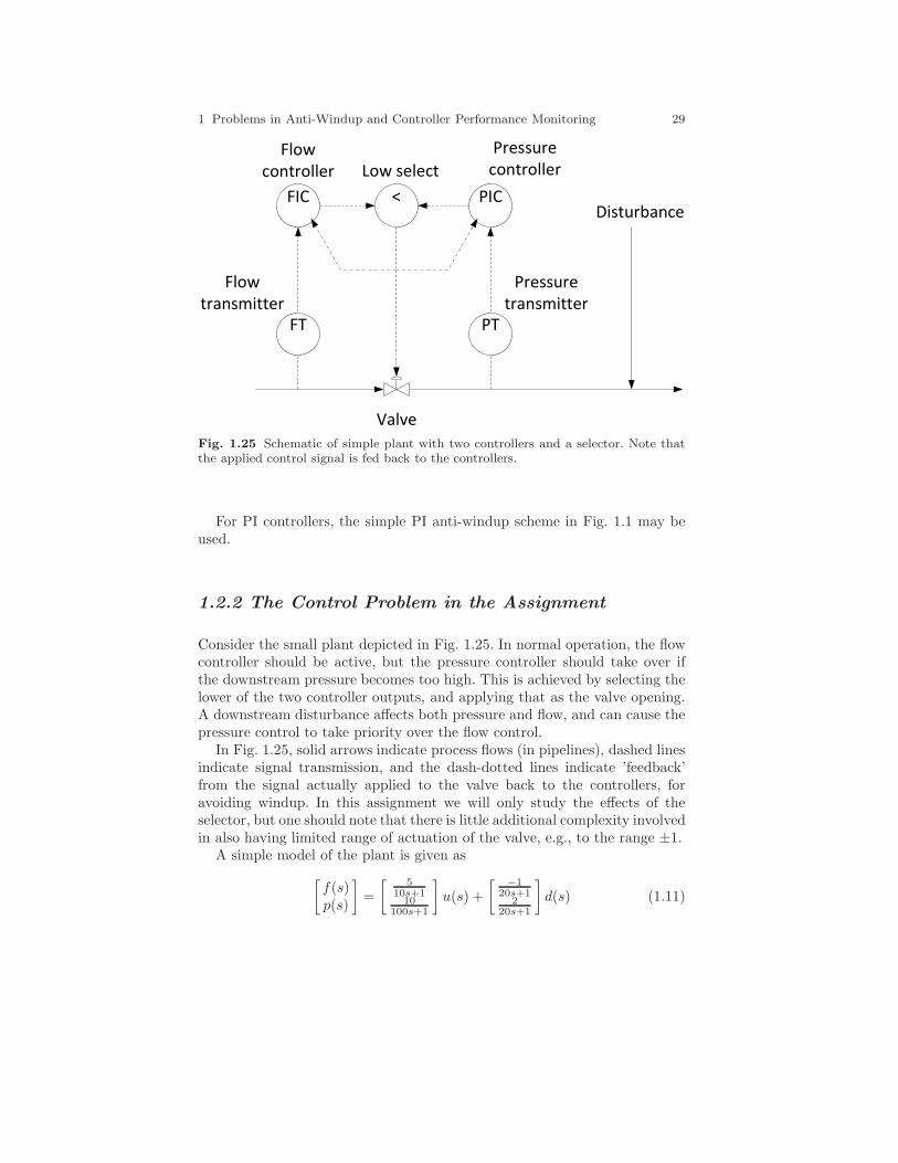
manipulated variable that is implemented is selected among the controlleroutputs. A simple example of selective control with pressure control on oneside and flow control on the other side of a valve is shown in Fig. 1.25.Normally one selects simply the highest or lowest value. A few points shouldbe made about this control structure:
• Clearly, a single manipulated variable can control only one controlled vari-able at the time, i.e., the only variable that is controlled at any instant isthe variable for which the corresponding controller output is implemented.It might appear strange to point out such a triviality, but discussions withseveral otherwise sensible engineers show that many have difficulty com-prehending this. Thus, one should consider with some care how such acontrol structure will work.
• The selection of the active controller is usually based on the controlleroutputs, not the controller inputs. Nevertheless the local operators andengineers often believe that the selection is based on the controller inputs,or that “the control switches when the a measurement passes its setpoint”.In principle, the selection of the active controller may also be based onthe controller inputs1. Some type of scaling will then often be necessary,in order to compare different types of physical quantities (e.g., comparingflowrates and pressures).
• If the controllers contain integral action, a severe problem that is similarto “reset windup” can occur unless special precautions are taken. The con-trollers that are not selected, should be reset (for normal PID controllerthis is done by adjusting the value of the controller integral) such that forthe present controller measurement, the presently selected manipulatedvariable value is obtained. Commonly used terms for this type of function-ality are “putting the inactive controllers in tracking mode” or “using afeedback relay”. This functionality should be implemented with some care,as faulty implementations which permanently lock the inactive controllersare known to have been used. On a digital control system, the controllersshould do the following for each sample interval:
1. Read in the process measurement.2. Calculate new controller output.3. The selector now selects the controller output to be implemented on the
manipulated variable.4. The controllers read in the implemented manipulated variable value.5. If the implemented manipulated variable value is different from the con-
troller output, the internal variables in the controller (typically the integralvalue) should be adjusted to obtain the currently implemented manipu-lated variable value as controller output, for the current process measure-ment.
1 Provided appropriate scaling of variables is used, the auctioneering control structuremay be a better alternative to using selective control with the selection based oncontroller inputs.
1 Problems in Anti-Windup and Controller Performance Monitoring 29
<
PT
PIC
FT
FICDisturbance
Pressure
controller
Flow
controller Low select
Flow
transmitter
Pressure
transmitter
Valve
Fig. 1.25 Schematic of simple plant with two controllers and a selector. Note thatthe applied control signal is fed back to the controllers.
For PI controllers, the simple PI anti-windup scheme in Fig. 1.1 may beused.
1.2.2 The Control Problem in the Assignment
Consider the small plant depicted in Fig. 1.25. In normal operation, the flowcontroller should be active, but the pressure controller should take over ifthe downstream pressure becomes too high. This is achieved by selecting thelower of the two controller outputs, and applying that as the valve opening.A downstream disturbance affects both pressure and flow, and can cause thepressure control to take priority over the flow control.
In Fig. 1.25, solid arrows indicate process flows (in pipelines), dashed linesindicate signal transmission, and the dash-dotted lines indicate ’feedback’from the signal actually applied to the valve back to the controllers, foravoiding windup. In this assignment we will only study the effects of theselector, but one should note that there is little additional complexity involvedin also having limited range of actuation of the valve, e.g., to the range ±1.
A simple model of the plant is given as
[f(s)p(s)
]=
[ 510s+110
100s+1
]u(s) +
[ −120s+1
220s+1
]d(s) (1.11)
30 Morten Hovd and Selvanathan Sivalingam
where f is the flowrate, p is the pressure, u is the valve position, and d isthe disturbance. Note that these variables, as always when using transferfunction models, are expressed in deviation variables, and thus both negativevalve positions, pressures and flowrates do make sense2.
1.2.3 Assignment
1. Model implementationImplement the a model of the plant in Simulink. The two controllers mayboth be given the setpoint zero. The disturbance should be modelled as asquare wave with period 500.
2. Controller tuningTune each of the PI controllers, without taking saturation or the selectorinto account. Any tuning methodology could be used (this should notbe very difficult anyway, since the plant in each of the loops is StrictlyPositive Real). However, completely unrealistic tunings should be avoided(i.e., for asymptotically stable plants like in this example, the closed looptime constant should not be orders of magnitude faster than the open looptime constant).
3. Simulation without anti-windupImplement the resulting PI controllers in Simulink – without accountingfor windup, and simulate with the disturbance active and both controllersoperating (i.e., with the selector).Comment on the results of the simulation.
4. Simulation with anti-windupImplement the PI controllers with anti-windup, and redo the simulation.Comment on the results and compare to the simulation results withoutanti-windup.
1.2.4 Solution
1.2.4.1 Model Implementation
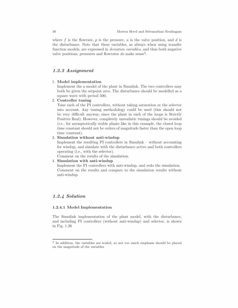
The Simulink implementation of the plant model, with the disturbance,and including PI controllers (without anti-windup) and selector, is shownin Fig. 1.26
2 In addition, the variables are scaled, so not too much emphasis should be placedon the magnitude of the variables
1 Problems in Anti-Windup and Controller Performance Monitoring 31
1.2.4.2 Controller Tuning
Not much effort has been put into the controller tuning. For each of thecontrollers, the integral time Ti has been set equal to the (dominant) timeconstant of the open loop, and a proportional gain of 1 is used. These tuningparameters are found to result in reasonable responses to setpoint changesfor each individual loop.
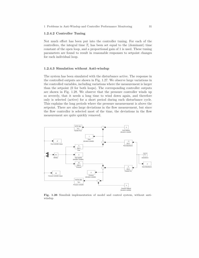
1.2.4.3 Simulation without Anti-windup
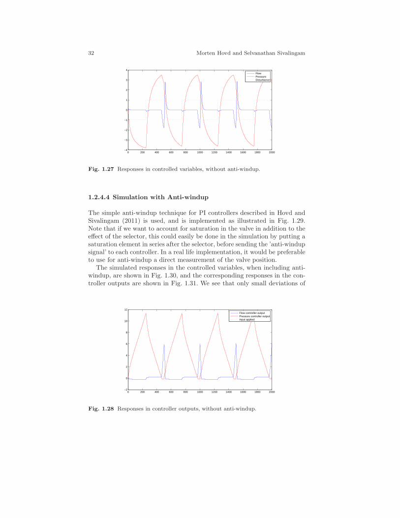
The system has been simulated with the disturbance active. The response inthe controlled outputs are shown in Fig. 1.27. We observe large variations inthe controlled variables, including variations where the measurement is largerthan the setpoint (0 for both loops). The corresponding controller outputsare shown in Fig. 1.28. We observe that the pressure controller winds upso severely, that it needs a long time to wind down again, and thereforeonly is selected (active) for a short period during each disturbance cycle.This explains the long periods where the pressure measurement is above thesetpoint. There are also large deviations in the flow measurement, but sincethe flow controller is selected most of the time, the deviations in the flowmeasurement are quite quickly removed.
Transfer Fcn1
Tif.s
kf*[Tif 1](s)
Transfer Fcn
2
20s+1
Save disturbance
d
Pressure setpoint(deviation variable)
0
Pressure controller output
up
Pressure controller
Tip.s
kp*[Tip 1](s)
Pressure(deviation variable)
p
Pressure
10
100s+1
MinMax
min
Input applied(deviation variable)
ur
Flow setpoint(deviation variable)
0
Flow disturbance
−1
20s+1Flow controller output
ufFlow
(deviation variable)
f
Flow
5
10s+1
Disturbance
Fig. 1.26 Simulink implementation of model and control system, without anti-windup
32 Morten Hovd and Selvanathan Sivalingam
0 200 400 600 800 1000 1200 1400 1600 1800 2000−4
−3
−2
−1
0
1
2
3
4
FlowPressureDisturbance
Fig. 1.27 Responses in controlled variables, without anti-windup.
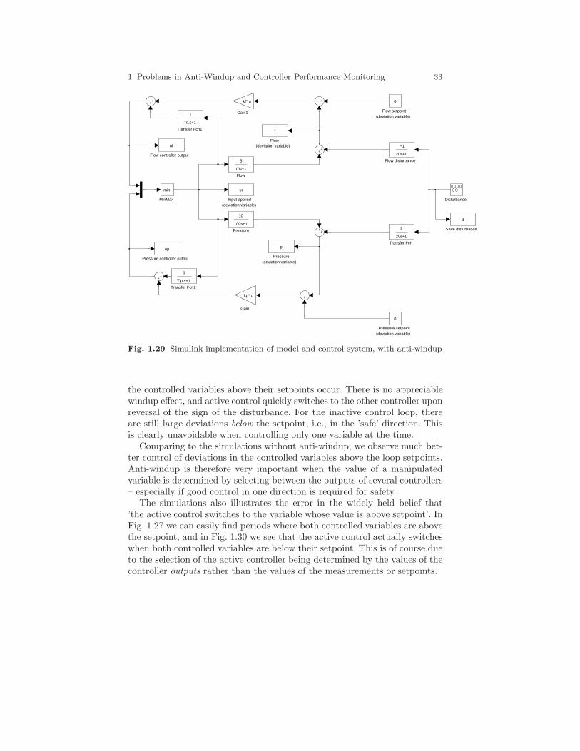
1.2.4.4 Simulation with Anti-windup
The simple anti-windup technique for PI controllers described in Hovd andSivalingam (2011) is used, and is implemented as illustrated in Fig. 1.29.Note that if we want to account for saturation in the valve in addition to theeffect of the selector, this could easily be done in the simulation by putting asaturation element in series after the selector, before sending the ’anti-windupsignal’ to each controller. In a real life implementation, it would be preferableto use for anti-windup a direct measurement of the valve position.
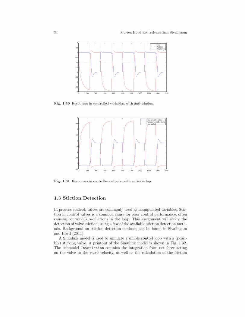
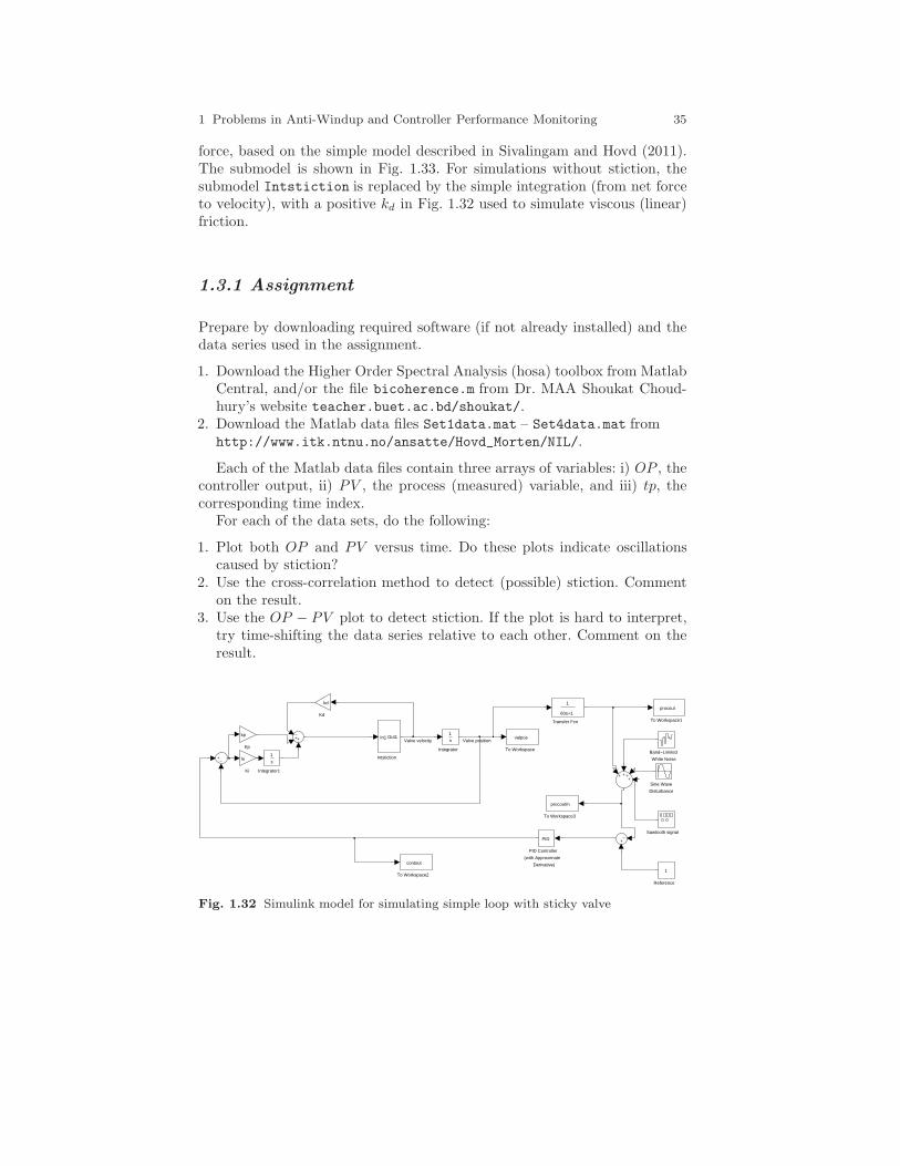
The simulated responses in the controlled variables, when including anti-windup, are shown in Fig. 1.30, and the corresponding responses in the con-troller outputs are shown in Fig. 1.31. We see that only small deviations of
0 200 400 600 800 1000 1200 1400 1600 1800 2000−2
0
2
4
6
8
10
12
Flow controller outputPressure controller outputInput applied
Fig. 1.28 Responses in controller outputs, without anti-windup.
1 Problems in Anti-Windup and Controller Performance Monitoring 33
Transfer Fcn2
1
Tip.s+1
Transfer Fcn1
1
Tif.s+1
Transfer Fcn
2
20s+1
Save disturbance
d
Pressure setpoint(deviation variable)
0
Pressure controller output
up
Pressure(deviation variable)
p
Pressure
10
100s+1
MinMax
min
Input applied(deviation variable)
ur
Gain1
kf* u
Gain
kp* u
Flow setpoint(deviation variable)
0
Flow disturbance
−1
20s+1Flow controller output
ufFlow
(deviation variable)
f
Flow
5
10s+1
Disturbance
Fig. 1.29 Simulink implementation of model and control system, with anti-windup
the controlled variables above their setpoints occur. There is no appreciablewindup effect, and active control quickly switches to the other controller uponreversal of the sign of the disturbance. For the inactive control loop, thereare still large deviations below the setpoint, i.e., in the ’safe’ direction. Thisis clearly unavoidable when controlling only one variable at the time.
Comparing to the simulations without anti-windup, we observe much bet-ter control of deviations in the controlled variables above the loop setpoints.Anti-windup is therefore very important when the value of a manipulatedvariable is determined by selecting between the outputs of several controllers– especially if good control in one direction is required for safety.
The simulations also illustrates the error in the widely held belief that’the active control switches to the variable whose value is above setpoint’. InFig. 1.27 we can easily find periods where both controlled variables are abovethe setpoint, and in Fig. 1.30 we see that the active control actually switcheswhen both controlled variables are below their setpoint. This is of course dueto the selection of the active controller being determined by the values of thecontroller outputs rather than the values of the measurements or setpoints.
34 Morten Hovd and Selvanathan Sivalingam
0 200 400 600 800 1000 1200 1400 1600 1800 2000−4
−3.5
−3
−2.5
−2
−1.5
−1
−0.5
0
0.5
1
FlowPressureDisturbance
Fig. 1.30 Responses in controlled variables, with anti-windup.
0 200 400 600 800 1000 1200 1400 1600 1800 2000−0.5
0
0.5
1
1.5
2
2.5
3
3.5
4
Flow controller outputPressure controller outputInput applied
Fig. 1.31 Responses in controller outputs, with anti-windup.
1.3 Stiction Detection
In process control, valves are commonly used as manipulated variables. Stic-tion in control valves is a common cause for poor control performance, oftencausing continuous oscillations in the loop. This assignment will study thedetection of valve stiction, using a few of the available stiction detection meth-ods. Background on stiction detection methods can be found in Sivalingamand Hovd (2011).
A Simulink model is used to simulate a simple control loop with a (possi-bly) sticking valve. A printout of the Simulink model is shown in Fig. 1.32.The submodel Intstiction contains the integration from net force actingon the valve to the valve velocity, as well as the calculation of the friction
1 Problems in Anti-Windup and Controller Performance Monitoring 35
force, based on the simple model described in Sivalingam and Hovd (2011).The submodel is shown in Fig. 1.33. For simulations without stiction, thesubmodel Intstiction is replaced by the simple integration (from net forceto velocity), with a positive kd in Fig. 1.32 used to simulate viscous (linear)friction.
1.3.1 Assignment
Prepare by downloading required software (if not already installed) and thedata series used in the assignment.
1. Download the Higher Order Spectral Analysis (hosa) toolbox from MatlabCentral, and/or the file bicoherence.m from Dr. MAA Shoukat Choud-hury’s website teacher.buet.ac.bd/shoukat/.
2. Download the Matlab data files Set1data.mat – Set4data.mat fromhttp://www.itk.ntnu.no/ansatte/Hovd_Morten/NIL/.
Each of the Matlab data files contain three arrays of variables: i) OP , thecontroller output, ii) PV , the process (measured) variable, and iii) tp, thecorresponding time index.
For each of the data sets, do the following:
1. Plot both OP and PV versus time. Do these plots indicate oscillationscaused by stiction?
2. Use the cross-correlation method to detect (possible) stiction. Commenton the result.
3. Use the OP − PV plot to detect stiction. If the plot is hard to interpret,try time-shifting the data series relative to each other. Comment on theresult.
Transfer Fcn
1
60s+1
To Workspace3
procoutm
To Workspace2
contout
To Workspace1
procout
To Workspace
valpos
Sine Wave
Disturbance
Sawtooth signal
Reference
1
PID Controller
(with Approximate
Derivative)
PID
Kp
kp
Ki
ki
Kd
kd
Intstiction
In1 Out1
Integrator1
1
s
Integrator
1
s
Band−Limited
White Noise
Valve velocity Valve position
Fig. 1.32 Simulink model for simulating simple loop with sticky valve
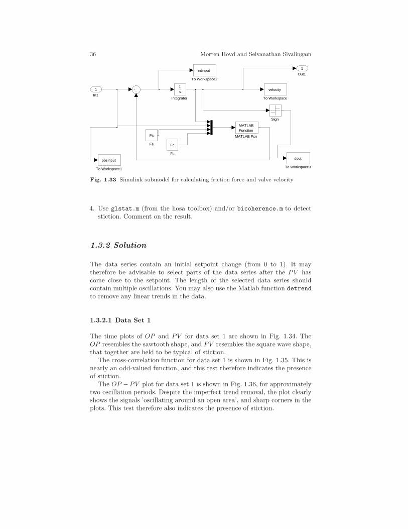
36 Morten Hovd and Selvanathan Sivalingam
Out1
1
To Workspace3
dout
To Workspace2
intinput
To Workspace1
posinput
To Workspace
velocity
Sign
MATLAB Fcn
MATLABFunction
Integrator
1s
Fs
Fs
Fc
Fc
In1
1
Fig. 1.33 Simulink submodel for calculating friction force and valve velocity
4. Use glstat.m (from the hosa toolbox) and/or bicoherence.m to detectstiction. Comment on the result.
1.3.2 Solution
The data series contain an initial setpoint change (from 0 to 1). It maytherefore be advisable to select parts of the data series after the PV hascome close to the setpoint. The length of the selected data series shouldcontain multiple oscillations. You may also use the Matlab function detrend
to remove any linear trends in the data.
1.3.2.1 Data Set 1
The time plots of OP and PV for data set 1 are shown in Fig. 1.34. TheOP resembles the sawtooth shape, and PV resembles the square wave shape,that together are held to be typical of stiction.
The cross-correlation function for data set 1 is shown in Fig. 1.35. This isnearly an odd-valued function, and this test therefore indicates the presenceof stiction.
The OP −PV plot for data set 1 is shown in Fig. 1.36, for approximatelytwo oscillation periods. Despite the imperfect trend removal, the plot clearlyshows the signals ’oscillating around an open area’, and sharp corners in theplots. This test therefore also indicates the presence of stiction.
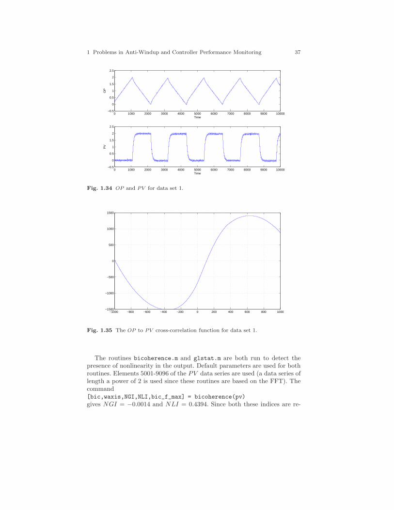
1 Problems in Anti-Windup and Controller Performance Monitoring 37
0 1000 2000 3000 4000 5000 6000 7000 8000 9000 10000−0.5
0
0.5
1
1.5
2
2.5
Time
OP
0 1000 2000 3000 4000 5000 6000 7000 8000 9000 10000−0.5
0
0.5
1
1.5
2
2.5
Time
PV
Fig. 1.34 OP and PV for data set 1.
−1000 −800 −600 −400 −200 0 200 400 600 800 1000−1500
−1000
−500
0
500
1000
1500
Fig. 1.35 The OP to PV cross-correlation function for data set 1.
The routines bicoherence.m and glstat.m are both run to detect thepresence of nonlinearity in the output. Default parameters are used for bothroutines. Elements 5001-9096 of the PV data series are used (a data series oflength a power of 2 is used since these routines are based on the FFT). Thecommand[bic,waxis,NGI,NLI,bic_f_max] = bicoherence(pv)
gives NGI = −0.0014 and NLI = 0.4394. Since both these indices are re-
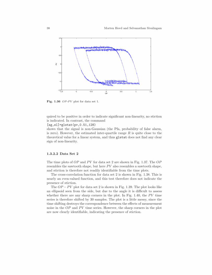
38 Morten Hovd and Selvanathan Sivalingam
−1.5 −1 −0.5 0 0.5 1 1.5−1.5
−1
−0.5
0
0.5
1
1.5
OP
PV
Fig. 1.36 OP -PV plot for data set 1.
quired to be positive in order to indicate significant non-linearity, no stictionis indicated. In contrast, the command[sg,sl]=glstat(pv,0.51,128)
shows that the signal is non-Gaussian (the Pfa, probability of false alarm,is zero). However, the estimated inter-quartile range R is quite close to thetheoretical value for a linear system, and thus glstat does not find any clearsign of non-linearity.
1.3.2.2 Data Set 2
The time plots of OP and PV for data set 2 are shown in Fig. 1.37. The OPresembles the sawtooth shape, but here PV also resembles a sawtooth shape,and stiction is therefore not readily identifiable from the time plots.
The cross-correlation function for data set 2 is shown in Fig. 1.38. This isnearly an even-valued function, and this test therefore does not indicate thepresence of stiction.
The OP −PV plot for data set 2 is shown in Fig. 1.39. The plot looks likean ellipsoid seen from the side, but due to the angle it is difficult to assesswhether there are any sharp corners in the plot. In Fig. 1.40, the PV timeseries is therefore shifted by 30 samples. The plot is a little messy, since thetime shifting destroys the correspondence between the effects of measurementnoise in the OP and PV time series. However, the sharp corners in the plotare now clearly identifiable, indicating the presence of stiction.
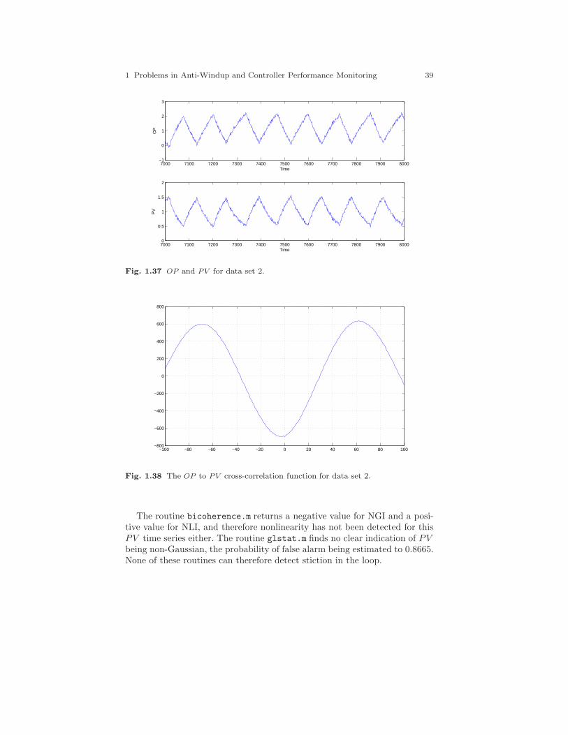
1 Problems in Anti-Windup and Controller Performance Monitoring 39
7000 7100 7200 7300 7400 7500 7600 7700 7800 7900 8000−1
0
1
2
3
Time
OP
7000 7100 7200 7300 7400 7500 7600 7700 7800 7900 80000
0.5
1
1.5
2
Time
PV
Fig. 1.37 OP and PV for data set 2.
−100 −80 −60 −40 −20 0 20 40 60 80 100−800
−600
−400
−200
0
200
400
600
800
Fig. 1.38 The OP to PV cross-correlation function for data set 2.
The routine bicoherence.m returns a negative value for NGI and a posi-tive value for NLI, and therefore nonlinearity has not been detected for thisPV time series either. The routine glstat.m finds no clear indication of PVbeing non-Gaussian, the probability of false alarm being estimated to 0.8665.None of these routines can therefore detect stiction in the loop.
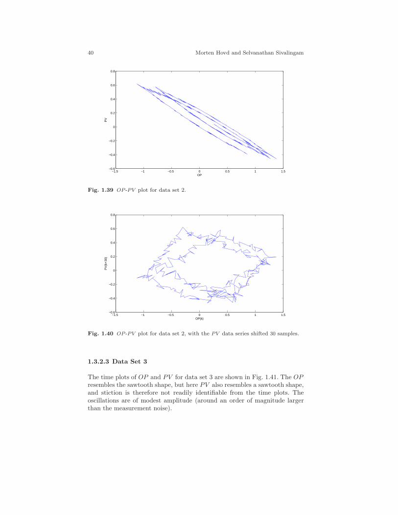
40 Morten Hovd and Selvanathan Sivalingam
−1.5 −1 −0.5 0 0.5 1 1.5−0.6
−0.4
−0.2
0
0.2
0.4
0.6
0.8
OP
PV
Fig. 1.39 OP -PV plot for data set 2.
−1.5 −1 −0.5 0 0.5 1 1.5−0.6
−0.4
−0.2
0
0.2
0.4
0.6
0.8
OP(k)
PV
(k+
30)
Fig. 1.40 OP -PV plot for data set 2, with the PV data series shifted 30 samples.
1.3.2.3 Data Set 3
The time plots of OP and PV for data set 3 are shown in Fig. 1.41. The OPresembles the sawtooth shape, but here PV also resembles a sawtooth shape,and stiction is therefore not readily identifiable from the time plots. Theoscillations are of modest amplitude (around an order of magnitude largerthan the measurement noise).
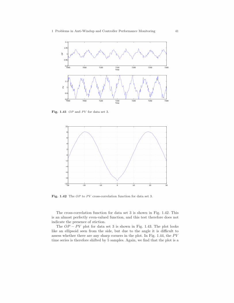
1 Problems in Anti-Windup and Controller Performance Monitoring 41
7000 7050 7100 7150 7200 7250 73000.9
0.95
1
1.05
1.1
Time
OP
7000 7050 7100 7150 7200 7250 73000.8
0.9
1
1.1
Time
PV
Fig. 1.41 OP and PV for data set 3.
−30 −20 −10 0 10 20 30−10
−8
−6
−4
−2
0
2
4
6
8
10
Fig. 1.42 The OP to PV cross-correlation function for data set 3.
The cross-correlation function for data set 3 is shown in Fig. 1.42. Thisis an almost perfectly even-valued function, and this test therefore does notindicate the presence of stiction.
The OP − PV plot for data set 3 is shown in Fig. 1.43. The plot lookslike an ellipsoid seen from the side, but due to the angle it is difficult toassess whether there are any sharp corners in the plot. In Fig. 1.44, the PVtime series is therefore shifted by 5 samples. Again, we find that the plot is a
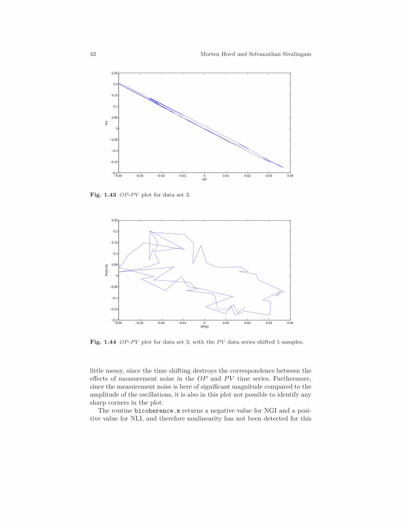
42 Morten Hovd and Selvanathan Sivalingam
−0.04 −0.03 −0.02 −0.01 0 0.01 0.02 0.03 0.04−0.2
−0.15
−0.1
−0.05
0
0.05
0.1
0.15
0.2
0.25
OP
PV
Fig. 1.43 OP -PV plot for data set 3.
−0.04 −0.03 −0.02 −0.01 0 0.01 0.02 0.03 0.04−0.2
−0.15
−0.1
−0.05
0
0.05
0.1
0.15
0.2
0.25
OP(k)
PV
(k+
5)
Fig. 1.44 OP -PV plot for data set 3, with the PV data series shifted 5 samples.
little messy, since the time shifting destroys the correspondence between theeffects of measurement noise in the OP and PV time series. Furthermore,since the measurement noise is here of significant magnitude compared to theamplitude of the oscillations, it is also in this plot not possible to identify anysharp corners in the plot.
The routine bicoherence.m returns a negative value for NGI and a posi-tive value for NLI, and therefore nonlinearity has not been detected for this
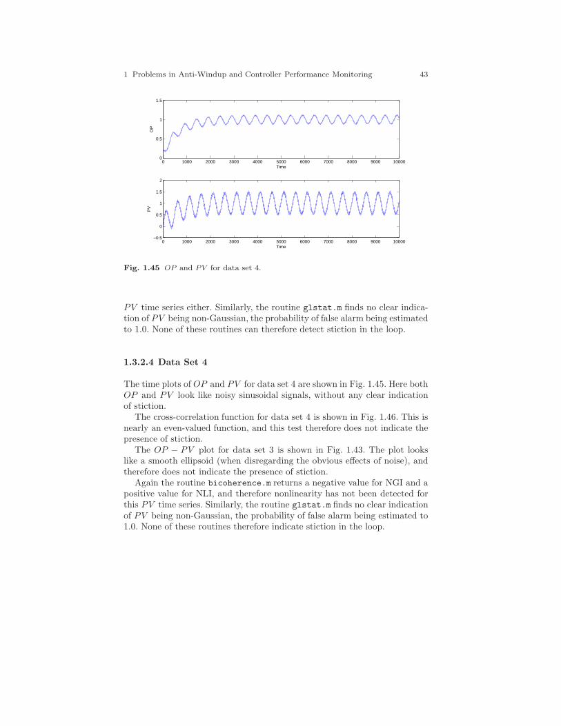
1 Problems in Anti-Windup and Controller Performance Monitoring 43
0 1000 2000 3000 4000 5000 6000 7000 8000 9000 100000
0.5
1
1.5
Time
OP
0 1000 2000 3000 4000 5000 6000 7000 8000 9000 10000−0.5
0
0.5
1
1.5
2
Time
PV
Fig. 1.45 OP and PV for data set 4.
PV time series either. Similarly, the routine glstat.m finds no clear indica-tion of PV being non-Gaussian, the probability of false alarm being estimatedto 1.0. None of these routines can therefore detect stiction in the loop.
1.3.2.4 Data Set 4
The time plots of OP and PV for data set 4 are shown in Fig. 1.45. Here bothOP and PV look like noisy sinusoidal signals, without any clear indicationof stiction.
The cross-correlation function for data set 4 is shown in Fig. 1.46. This isnearly an even-valued function, and this test therefore does not indicate thepresence of stiction.
The OP − PV plot for data set 3 is shown in Fig. 1.43. The plot lookslike a smooth ellipsoid (when disregarding the obvious effects of noise), andtherefore does not indicate the presence of stiction.
Again the routine bicoherence.m returns a negative value for NGI and apositive value for NLI, and therefore nonlinearity has not been detected forthis PV time series. Similarly, the routine glstat.m finds no clear indicationof PV being non-Gaussian, the probability of false alarm being estimated to1.0. None of these routines therefore indicate stiction in the loop.
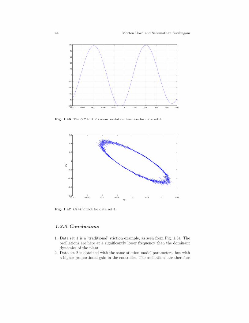
44 Morten Hovd and Selvanathan Sivalingam
−500 −400 −300 −200 −100 0 100 200 300 400 500−100
−80
−60
−40
−20
0
20
40
60
80
100
Fig. 1.46 The OP to PV cross-correlation function for data set 4.
−0.2 −0.15 −0.1 −0.05 0 0.05 0.1 0.15−0.8
−0.6
−0.4
−0.2
0
0.2
0.4
0.6
OP
PV
Fig. 1.47 OP -PV plot for data set 4.
1.3.3 Conclusions
1. Data set 1 is a ’traditional’ stiction example, as seen from Fig. 1.34. Theoscillations are here at a significantly lower frequency than the dominantdynamics of the plant.
2. Data set 2 is obtained with the same stiction model parameters, but witha higher proportional gain in the controller. The oscillations are therefore
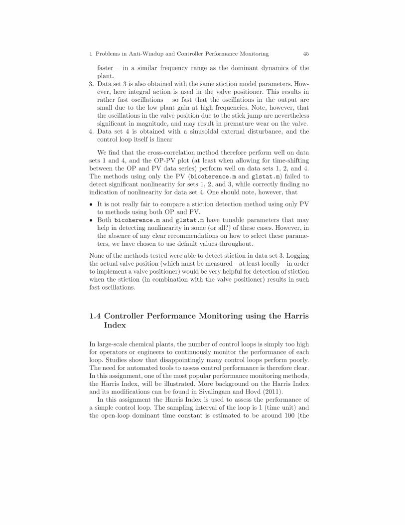
1 Problems in Anti-Windup and Controller Performance Monitoring 45
faster – in a similar frequency range as the dominant dynamics of theplant.
3. Data set 3 is also obtained with the same stiction model parameters. How-ever, here integral action is used in the valve positioner. This results inrather fast oscillations – so fast that the oscillations in the output aresmall due to the low plant gain at high frequencies. Note, however, thatthe oscillations in the valve position due to the stick jump are neverthelesssignificant in magnitude, and may result in premature wear on the valve.
4. Data set 4 is obtained with a sinusoidal external disturbance, and thecontrol loop itself is linear
We find that the cross-correlation method therefore perform well on datasets 1 and 4, and the OP-PV plot (at least when allowing for time-shiftingbetween the OP and PV data series) perform well on data sets 1, 2, and 4.The methods using only the PV (bicoherence.m and glstat.m) failed todetect significant nonlinearity for sets 1, 2, and 3, while correctly finding noindication of nonlinearity for data set 4. One should note, however, that
• It is not really fair to compare a stiction detection method using only PVto methods using both OP and PV.
• Both bicoherence.m and glstat.m have tunable parameters that mayhelp in detecting nonlinearity in some (or all?) of these cases. However, inthe absence of any clear recommendations on how to select these parame-ters, we have chosen to use default values throughout.
None of the methods tested were able to detect stiction in data set 3. Loggingthe actual valve position (which must be measured – at least locally – in orderto implement a valve positioner) would be very helpful for detection of stictionwhen the stiction (in combination with the valve positioner) results in suchfast oscillations.
1.4 Controller Performance Monitoring using the HarrisIndex
In large-scale chemical plants, the number of control loops is simply too highfor operators or engineers to continuously monitor the performance of eachloop. Studies show that disappointingly many control loops perform poorly.The need for automated tools to assess control performance is therefore clear.In this assignment, one of the most popular performance monitoring methods,the Harris Index, will be illustrated. More background on the Harris Indexand its modifications can be found in Sivalingam and Hovd (2011).
In this assignment the Harris Index is used to assess the performance ofa simple control loop. The sampling interval of the loop is 1 (time unit) andthe open-loop dominant time constant is estimated to be around 100 (the
46 Morten Hovd and Selvanathan Sivalingam
knowledge of the dominant time constant is not known for calculating theHarris Index, but is used in one of the more common modifications of theindex). The plant is strictly proper, but there is otherwise no time delay frominput to output, i.e., h(0) = 0, h(1) 6= 0 where h(k) is the impulse responsecoefficient for lag k. The plant is open loop stable and has no zeros outsidethe unit disk.
1.4.1 Assignment
1. Download the Matlab data file cpmsim.mat fromhttp://www.itk.ntnu.no/ansatte/Hovd_Morten/NIL/. The file containsthe measurement (OP) of a control loop. Since the setpoint is 0, the mea-surement and control offset are equivalent.
2. Calculate the Harris Index (or Normalized Harris Index) for the controlloop. Is there scope for significant improvements in control performance?
3. Select a reasonable value for the desired closed loop dominant time con-stant. Instead of the minimum variance benchmark used in the HarrisIndex, use a modified benchmark reflecting a desired closed loop time con-stant to assess control performance.
The calculations involved are relatively simple, and appropriate Matlabroutines may be programmed by the student. Alternatively, the Matlab rou-tines ar and impulse may be useful.
1.4.2 Solution
First the mean of the data series OP is removed with the command opd
= detrend(op,’constant’). Next, a 10th-order auto-regressive model fromthe (unmeasured) disturbance to the controlled variable is identified usingthe command mod=ar(opd,10). The routine ar() finds parameters for themodel
y(k) + α1y(k − 1) + α2y(k − 2) + · · ·+ α(10)y(k − 10) = a(k) (1.12)
mA(q−1)y(k) = d(k)
where y(k) is the measurement at time k, and a(k) is the (unmeasured) distur-bance. Note that the leading coefficient of the polynomial A(q−1), α(0) = 1.The coefficients of the polynomial A(q−1) are found in mod.a, and the es-timated variance of a(k) is found in mod.NoiseVariance. The AR modelis converted to an impulse response model by simple polynomial long divi-
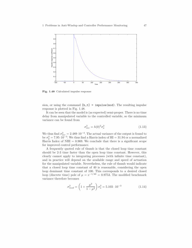
1 Problems in Anti-Windup and Controller Performance Monitoring 47
−100 −50 0 50 100 150 200 250 300 3500
0.1
0.2
0.3
0.4
0.5
0.6
0.7
0.8
0.9
1
Time
Impu
lse
resp
onse
coe
ffici
ent
Fig. 1.48 Calculated impulse response
sion, or using the command [h,t] = impulse(mod). The resulting impulseresponse is plotted in Fig. 1.48.
It can be seen that the model is (as expected) semi-proper. There is no timedelay from manipulated variable to the controlled variable, so the minimumvariance can be found from
σ2mv = h(0)2σ2
a (1.13)
We thus find σ2mv = 2.489·10−4. The actual variance of the output is found to
be σ2y = 7.95 ·10−3. We thus find a Harris index of HI = 31.94 or a normalized
Harris Index of NHI = 0.969. We conclude that there is a significant scopefor improved control performance.
A frequently quoted rule of thumb is that the closed loop time constantshould be 2-3 time faster than the open loop time constant. However, thisclearly cannot apply to integrating processes (with infinite time constant),and in practice will depend on the available range and speed of actuationfor the manipulated variable. Nevertheless, the rule of thumb would indicatethat a closed loop time constant of 40 is reasonable, considering the openloop dominant time constant of 100. This corresponds to a desired closedloop (discrete time) pole of µ = e−1/40 = 0.9753. The modified benchmarkvariance therefore becomes
σ2mod =
(1 +
µ2
1− µ2
)σ2a = 5.103 · 10−3 (1.14)

48 Morten Hovd and Selvanathan Sivalingam
With this modified benchmark variance, we find a modified Harris index ofHImod = 1.49, or NHImod = 0.327. Thus, with the chosen closed loop timeconstant as basis for comparison, the motivation for retuning the controlleris significantly reduced, as the observed variance is not much larger than the’acceptable’ variance.
Acknowledgements The authors are pleased to acknowledge the financial supportby a grant No. NIL-I-007-d from Iceland, Liechtenstein and Norway through the EEAFinancial Mechanism and the Norwegian Financial Mechanism.
The contributions of Anders Fougner and Anders Willersrud in preparing the anti-windup assignment are also gratefully acknowledged.
References
Hanus R, Kinnaert M, Henrotte JL (1987) Conditioning technique, a general anti-windup and bumpless transfer method. Automatica 23(6):729–739
Hovd M, Sivalingam S (2011) A short introduction to anti-windup. In: Huba M,Skogestad S, Fikar M, Hovd M, Johansen TA, Rohal’-Ilkiv B (eds) Selected Top-ics on Constrained and Nonlinear Control. Textbook, STU Bratislava – NTNUTrondheim
Sivalingam S, Hovd M (2011) Controller performance monitoring and assessment.In: Huba M, Skogestad S, Fikar M, Hovd M, Johansen TA, Rohal’-Ilkiv B (eds)Selected Topics on Constrained and Nonlinear Control. Textbook, STU Bratislava– NTNU Trondheim
Skogestad S, Postlethwaite I (2005) Multivariable Feedback Control. Analysis andDesign. John Wiley & Sons Ltd, Chichester, England
Wade HL (1997) Inverted decoupling – a neglected technique. ISA Transactions 36:3–10

1 Problems in Anti-Windup and Controller Performance Monitoring 49
Comments – Remarks

50 Morten Hovd and Selvanathan Sivalingam
Comments – Remarks

1 Problems in Anti-Windup and Controller Performance Monitoring 51
Comments – Remarks

52 Morten Hovd and Selvanathan Sivalingam
Comments – Remarks
Chapter 2
Optimal Use of Measurements forControl, Optimization and Estimationusing the Loss Method: Summary ofExisting Results and Some New
Sigurd Skogestad and Ramprasad Yelchuru and Johannes Jaschke
Abstract The objective of this chapter is to study the optimal use of mea-surements and measurements combinations, c = Hy in optimization andestimation based on the loss method.
2.1 Introduction
In this paper we consider a (steady-state) unconstrained quadratic optimiza-tion problem with linear measurement relationships. The main objective isto find a linear measurement combination, c = Hy, such that control ofthese indirectly leads to close-to-optimal operation with a small loss L, inspite of unknown disturbances, d, and measurement noise (error), ny. If theoriginal optimization problem is constrained, then we assume that any ac-tive constraints are kept constant (controlled) and we consider the lower-dimensional unconstrained subspace. Depending on the disturbance rangeconsidered, there may be several constrained regions, and the procedure offinding H needs to be repeated in each constrained region. Switching be-tween the regions will then be needed, and we will show that monitoring thecontrolled variables c = Hy in neighboring regions can be used for switching.
Sigurd SkogestadDepartment of Chemical Engineering, Norwegian University of Science and Technol-ogy in Trondheim, Norway, e-mail: [email protected]
Ramprasad YelchuruDepartment of Chemical Engineering, Norwegian University of Science and Technol-ogy in Trondheim, Norway, e-mail: [email protected]
Johannes JaschkeDepartment of Chemical Engineering, Norwegian University of Science and Technol-ogy in Trondheim, Norway, e-mail: [email protected]
53
54 Sigurd Skogestad and Ramprasad Yelchuru and Johannes Jaschke
What we here call the “loss method” is the same as what is called the“exact local method” in these papers (Halvorsen et al (2003); Alstad et al(2009)).
The new material in this summary paper is mainly related to using data(Y ,X) as the basis, and for example, to use the “loss”method for regression,see section 5, data approach 1 and 2.
2.2 Problem Formulation
2.2.1 Classification of Variables
• u - inputs (degrees of freedom) for optimization and control (it does notactually matter what they are as long as they form an independent set)
• d - disturbances, including parameter changes.• y - all available measurements (will later call a subset of these for x in ac-
cordance with statistics notation). The manipulated variables (MVs, oftenthe same as the inputs u) are generally included in the measurement sety. This will allow, for example, for simple control policies where the inputsare kept constant. Of course, the set y also includes measured disturbances(dm, a subset of d).
• ny - measurement noise (error) for y, ym = y + ny.• p - prices = weights that enter into cost function (do not affect y)
2.2.2 Cost Function
The objective is to choose the input u to minimize the quadratic cost function
J(u,d) = uTQ1u+ dTQ2d+ uTQ3d (2.1)
Note that for simplicity, we have not included linear terms in the cost func-tion. Any linear term in u can be removed by shifting the zero point for u
to be at the optimal point. On the other hand, a linear term in d cannot becounteracted by choosing the input u, so excluding it does not change thesolution. The same applies to any constant term in the cost.
If we compare (2.1), with a second-order Taylor series expansion of thecost around a nominal point (u∗,d∗), then we have that
Q1 =1
2J∗
uu,Q2 = J∗ud,Q3 =
1
2J∗
dd
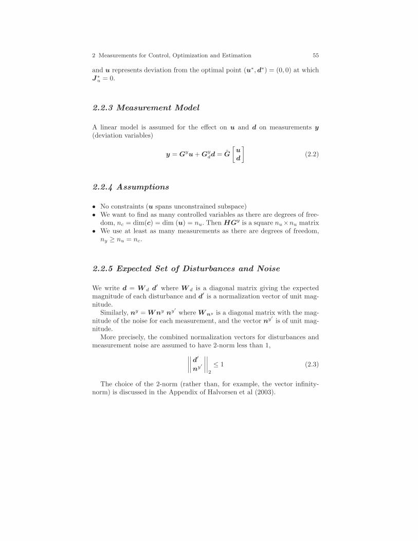
2 Measurements for Control, Optimization and Estimation 55
and u represents deviation from the optimal point (u∗,d∗) = (0, 0) at whichJ∗
u = 0.
2.2.3 Measurement Model
A linear model is assumed for the effect on u and d on measurements y
(deviation variables)
y = Gyu+Gydd = G
[u
d
](2.2)
2.2.4 Assumptions
• No constraints (u spans unconstrained subspace)• We want to find as many controlled variables as there are degrees of free-
dom, nc = dim(c) = dim (u) = nu. Then HGy is a square nu×nu matrix• We use at least as many measurements as there are degrees of freedom,
ny ≥ nu = nc.
2.2.5 Expected Set of Disturbances and Noise
We write d = W d d′ where W d is a diagonal matrix giving the expectedmagnitude of each disturbance and d′ is a normalization vector of unit mag-nitude.
Similarly, ny = Wny ny′
where Wny is a diagonal matrix with the mag-nitude of the noise for each measurement, and the vector ny′
is of unit mag-nitude.
More precisely, the combined normalization vectors for disturbances andmeasurement noise are assumed to have 2-norm less than 1,
∣∣∣∣∣∣∣∣d′
ny′
∣∣∣∣∣∣∣∣2
≤ 1 (2.3)
The choice of the 2-norm (rather than, for example, the vector infinity-norm) is discussed in the Appendix of Halvorsen et al (2003).
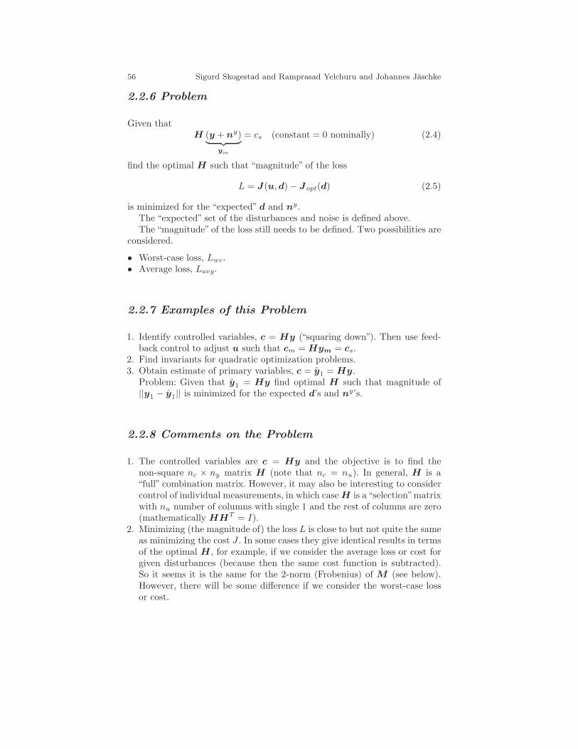
56 Sigurd Skogestad and Ramprasad Yelchuru and Johannes Jaschke
2.2.6 Problem
Given thatH (y + ny)︸ ︷︷ ︸
ym
= cs (constant = 0 nominally) (2.4)
find the optimal H such that “magnitude” of the loss
L = J(u,d)− Jopt(d) (2.5)
is minimized for the “expected” d and ny.The “expected” set of the disturbances and noise is defined above.The “magnitude” of the loss still needs to be defined. Two possibilities are
considered.
• Worst-case loss, Lwc.• Average loss, Lavg.
2.2.7 Examples of this Problem
1. Identify controlled variables, c = Hy (“squaring down”). Then use feed-back control to adjust u such that cm = Hym = cs.
2. Find invariants for quadratic optimization problems.3. Obtain estimate of primary variables, c = y1 = Hy.
Problem: Given that y1 = Hy find optimal H such that magnitude of||y1 − y1|| is minimized for the expected d’s and ny’s.
2.2.8 Comments on the Problem
1. The controlled variables are c = Hy and the objective is to find thenon-square nc × ny matrix H (note that nc = nu). In general, H is a“full” combination matrix. However, it may also be interesting to considercontrol of individual measurements, in which caseH is a“selection”matrixwith nu number of columns with single 1 and the rest of columns are zero(mathematically HHT = I).
2. Minimizing (the magnitude of) the loss L is close to but not quite the sameas minimizing the cost J . In some cases they give identical results in termsof the optimal H, for example, if we consider the average loss or cost forgiven disturbances (because then the same cost function is subtracted).So it seems it is the same for the 2-norm (Frobenius) of M (see below).However, there will be some difference if we consider the worst-case lossor cost.
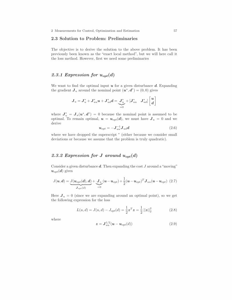
2 Measurements for Control, Optimization and Estimation 57
2.3 Solution to Problem: Preliminaries
The objective is to derive the solution to the above problem. It has beenpreviously been known as the “exact local method”, but we will here call itthe loss method. However, first we need some preliminaries
2.3.1 Expression for uopt(d)
We want to find the optimal input u for a given disturbance d. Expandingthe gradient Ju around the nominal point (u∗,d∗) = (0, 0) gives
Ju = J∗u + J∗
uuu+ J∗udd = J∗
u︸︷︷︸=0
+ [J∗uu J∗
ud]
[u
d
]
where J∗u = Ju(u
∗,d∗) = 0 because the nominal point is assumed to beoptimal. To remain optimal, u = uopt(d), we must have Ju = 0 and wederive
uopt = −J−1uuJudd (2.6)
where we have dropped the superscript ∗ (either because we consider smalldeviations or because we assume that the problem is truly quadratic).
2.3.2 Expression for J around uopt(d)
Consider a given disturbance d. Then expanding the cost J around a“moving”uopt(d) gives
J(u,d) = J(uopt(d),d)︸ ︷︷ ︸Jopt(d)
+ Ju︸︷︷︸=0
(u−uopt)+1
2(u−uopt)
TJuu(u−uopt) (2.7)
Here Ju = 0 (since we are expanding around an optimal point), so we getthe following expression for the loss
L(u, d) = J(u, d)− Jopt(d) =1
2zTz =
1
2||z||22 (2.8)
wherez = J1/2
uu (u− uopt(d)) (2.9)

58 Sigurd Skogestad and Ramprasad Yelchuru and Johannes Jaschke
2.3.3 Expression for Ju around Moving uopt(d)
A similar expansion, but now of the gradient gives
Ju = Ju(uopt)︸ ︷︷ ︸=0
+Juu(u− uopt) = Juu(u− uopt) (2.10)
Combining this with (2.9) gives z = J−1/2uu Ju and we have the “Johannes
expression” for the loss
L(u, d) = J(u, d)− Jopt(d) =1
2
∣∣∣∣∣∣J−1/2
uu Ju
∣∣∣∣∣∣2
2(2.11)
From these expressions we see that minimizing the loss L is equivalent to
minimizing ||z||2, which is equivalent to minimizing∣∣∣∣∣∣J1/2
uu (u − uopt)∣∣∣∣∣∣2or
∣∣∣∣∣∣J− 1
2uu Ju
∣∣∣∣∣∣2.
Thus, we have the important conclusion that minimizing the loss is equiv-alent to minimizing the weighted 2-norm of the gradient Ju, with the weightbeing given by the matrix J−1/2
uu . However, for the “normal” case when thereare no restrictions (like fixing some elements to zero) on the matrix H , we
will show below that the weight J−1/2uu does not have any effect on the optimal
H.
2.3.4 Optimal Sensitivities
Note from (2.6) that we can write uopt = F ud where F u = −J−1uuJud. More
generally, we can writeyopt = Fd (2.12)
where F is the optimal sensitivity of the outputs (measurements) with respectto the disturbances. Here, F can be obtained using (2.2) and (2.6),
yopt = Gyuopt +Gydd = (−GyJ−1
uuJud +Gyd)d
that is,F = (−GyJ−1
uuJud +Gyd) (2.13)
However, Juu can be difficult to obtain, especially if one relies on numericalmethods, and also taking the difference can introduce numerical inaccuracy.Thus, for practical use it is often better to obtain F from its definition,F = dyopt/dd, by numerically reoptimizing the model for the disturbances.
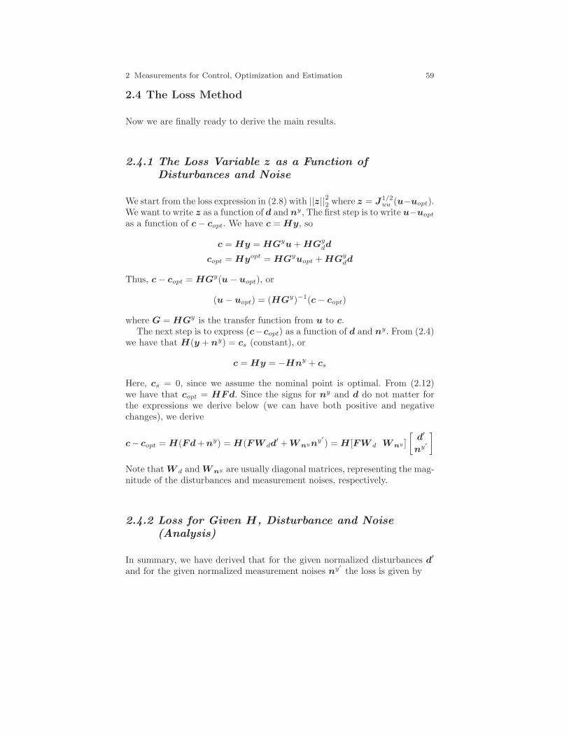
2 Measurements for Control, Optimization and Estimation 59
2.4 The Loss Method
Now we are finally ready to derive the main results.
2.4.1 The Loss Variable z as a Function ofDisturbances and Noise
We start from the loss expression in (2.8) with ||z||22 where z = J1/2uu (u−uopt).
We want to write z as a function of d and ny, The first step is to write u−uopt
as a function of c− copt. We have c = Hy, so
c = Hy = HGyu+HGydd
copt = Hyopt = HGyuopt +HGydd
Thus, c− copt = HGy(u− uopt), or
(u − uopt) = (HGy)−1(c− copt)
where G = HGy is the transfer function from u to c.The next step is to express (c−copt) as a function of d and ny. From (2.4)
we have that H(y + ny) = cs (constant), or
c = Hy = −Hny + cs
Here, cs = 0, since we assume the nominal point is optimal. From (2.12)we have that copt = HFd. Since the signs for ny and d do not matter forthe expressions we derive below (we can have both positive and negativechanges), we derive
c− copt = H(Fd+ny) = H(FW dd′ +Wnyny′
) = H [FW d Wny ]
[d′
ny′
]
Note that W d and Wny are usually diagonal matrices, representing the mag-nitude of the disturbances and measurement noises, respectively.
2.4.2 Loss for Given H, Disturbance and Noise(Analysis)
In summary, we have derived that for the given normalized disturbances d′
and for the given normalized measurement noises ny′
the loss is given by
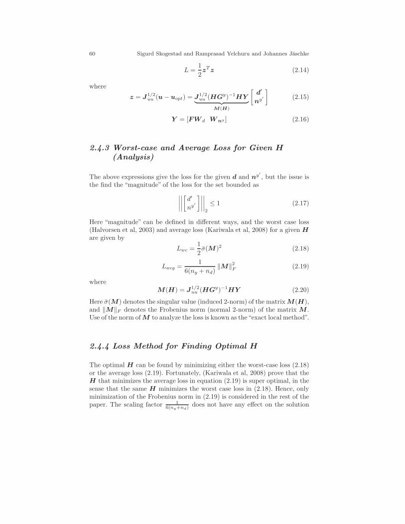
60 Sigurd Skogestad and Ramprasad Yelchuru and Johannes Jaschke
L =1
2zTz (2.14)
where
z = J1/2uu (u − uopt) = J1/2
uu (HGy)−1HY︸ ︷︷ ︸M(H)
[d′
ny′
](2.15)
Y = [FW d Wny ] (2.16)
2.4.3 Worst-case and Average Loss for Given H
(Analysis)
The above expressions give the loss for the given d and ny′
, but the issue isthe find the “magnitude” of the loss for the set bounded as
∣∣∣∣∣∣∣∣[d′
ny′
]∣∣∣∣∣∣∣∣2
≤ 1 (2.17)
Here “magnitude” can be defined in different ways, and the worst case loss(Halvorsen et al, 2003) and average loss (Kariwala et al, 2008) for a given H
are given by
Lwc =1
2σ(M )2 (2.18)
Lavg =1
6(ny + nd)‖M‖2F (2.19)
whereM(H) = J1/2
uu (HGy)−1HY (2.20)
Here σ(M) denotes the singular value (induced 2-norm) of the matrixM(H),and ‖M‖F denotes the Frobenius norm (normal 2-norm) of the matrix M .Use of the norm ofM to analyze the loss is known as the“exact local method”.
2.4.4 Loss Method for Finding Optimal H
The optimal H can be found by minimizing either the worst-case loss (2.18)or the average loss (2.19). Fortunately, (Kariwala et al, 2008) prove that theH that minimizes the average loss in equation (2.19) is super optimal, in thesense that the same H minimizes the worst case loss in (2.18). Hence, onlyminimization of the Frobenius norm in (2.19) is considered in the rest of thepaper. The scaling factor 1
6(ny+nd)does not have any effect on the solution
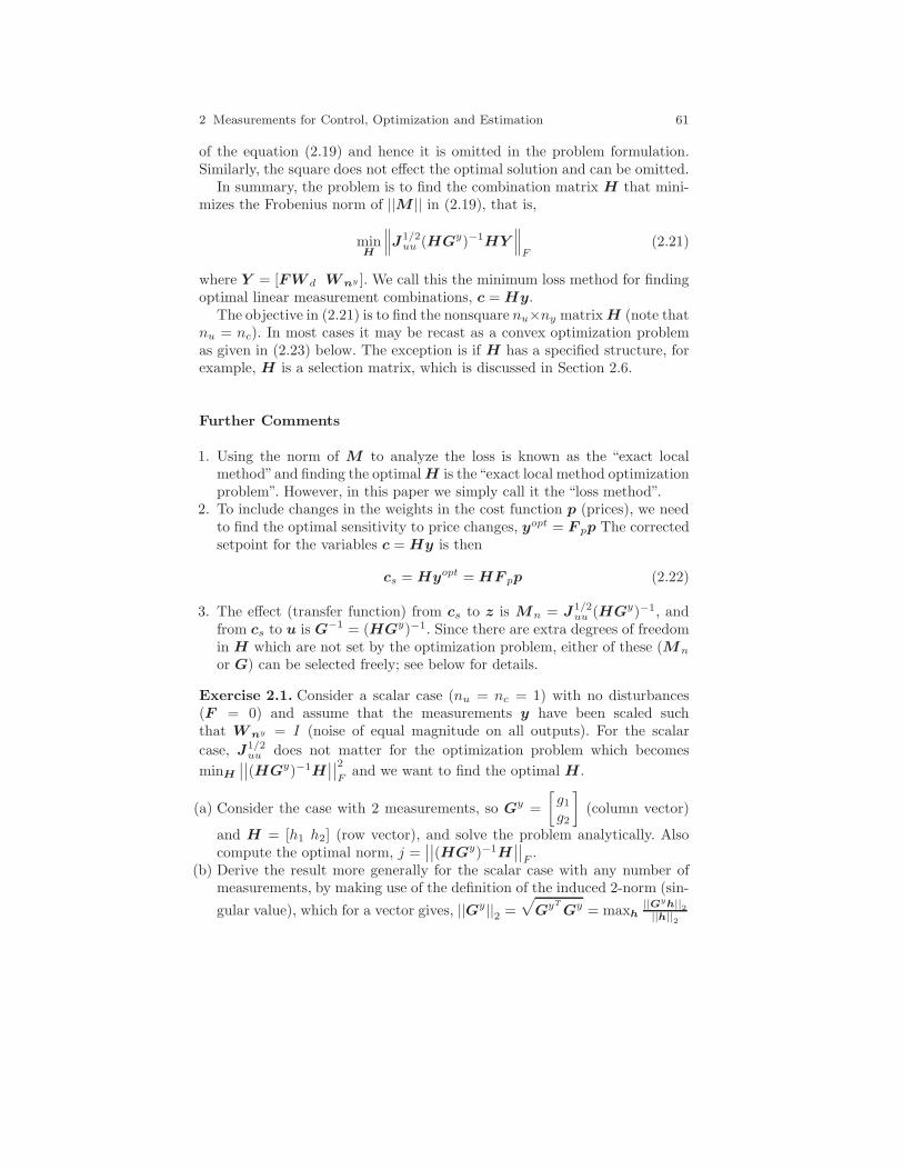
2 Measurements for Control, Optimization and Estimation 61
of the equation (2.19) and hence it is omitted in the problem formulation.Similarly, the square does not effect the optimal solution and can be omitted.
In summary, the problem is to find the combination matrix H that mini-mizes the Frobenius norm of ||M || in (2.19), that is,
minH
∥∥∥J1/2uu (HGy)−1HY
∥∥∥F
(2.21)
where Y = [FW d Wny ]. We call this the minimum loss method for findingoptimal linear measurement combinations, c = Hy.
The objective in (2.21) is to find the nonsquare nu×ny matrixH (note thatnu = nc). In most cases it may be recast as a convex optimization problemas given in (2.23) below. The exception is if H has a specified structure, forexample, H is a selection matrix, which is discussed in Section 2.6.
Further Comments
1. Using the norm of M to analyze the loss is known as the “exact localmethod”and finding the optimalH is the“exact local method optimizationproblem”. However, in this paper we simply call it the “loss method”.
2. To include changes in the weights in the cost function p (prices), we needto find the optimal sensitivity to price changes, yopt = F pp The correctedsetpoint for the variables c = Hy is then
cs = Hyopt = HF pp (2.22)
3. The effect (transfer function) from cs to z is Mn = J1/2uu (HGy)−1, and
from cs to u is G−1 = (HGy)−1. Since there are extra degrees of freedomin H which are not set by the optimization problem, either of these (Mn
or G) can be selected freely; see below for details.
Exercise 2.1. Consider a scalar case (nu = nc = 1) with no disturbances(F = 0) and assume that the measurements y have been scaled suchthat Wny = I (noise of equal magnitude on all outputs). For the scalar
case, J1/2uu does not matter for the optimization problem which becomes
minH∣∣∣∣(HGy)−1H
∣∣∣∣2Fand we want to find the optimal H .
(a) Consider the case with 2 measurements, so Gy =
[g1g2
](column vector)
and H = [h1 h2] (row vector), and solve the problem analytically. Alsocompute the optimal norm, j =
∣∣∣∣(HGy)−1H∣∣∣∣F.
(b) Derive the result more generally for the scalar case with any number ofmeasurements, by making use of the definition of the induced 2-norm (sin-
gular value), which for a vector gives, ||Gy||2 =√GyT
Gy = maxh||Gyh||2||h||2
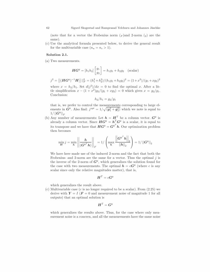
62 Sigurd Skogestad and Ramprasad Yelchuru and Johannes Jaschke
(note that for a vector the Frobenius norm (F )and 2-norm (2) are thesame).
(c) Use the analytical formula presented below, to derive the general resultfor the multivariable case (nu = nc > 1).
Solution 2.1.
(a) Two measurements.
HGy = [h1h2]
[g1g2
]= h1g1 + h2g2 (scalar)
j2 =∣∣∣∣(HGy)−1H
∣∣∣∣ ||2F = (h21+h2
2)/(h1g1+h2g2)2 = (1+x2)/(g1+xg2)
2
where x = h2/h1. Set d(j2)/dx = 0 to find the optimal x. After a lit-tle simplification x − (1 + x2)g2/(g1 + xg2) = 0 which gives x = g2/g1.Conclusion:
h2/h1 = g2/g1
that is, we prefer to control the measurements corresponding to large el-ements in Gy. Also find: jopt = 1/
√(g2
1 + g22) which we note is equal to
1/ ||Gy||F(b) Any number of measurements: Let h = HT be a column vector. Gy is
already a column vector. Since HGy = hTGy is a scalar, it is equal to
its transpose and we have that HGy = GyT
h. Our optimization problemthen becomes
minH
j = minh
∣∣∣∣∣
∣∣∣∣∣h
(GyT
h)
∣∣∣∣∣
∣∣∣∣∣F
= 1/
max
h
∣∣∣∣∣∣GyT
h
∣∣∣∣∣∣2
||h||2
= 1/ ||Gy||2
We have here made use of the induced 2-norm and the fact that both theFrobenius- and 2-norm are the same for a vector. Thus the optimal j isthe inverse of the 2-norm of Gy, which generalizes the solution found forthe case with two measurements. The optimal h = cGy (where c is anyscalar since only the relative magnitudes matter), that is,
HT = cGy
which generalizes the result above.(c) Multivariable case (c is no longer required to be a scalar). From (2.25) we
derive with Y = I (F = 0 and measurement noise of magnitude 1 for alloutputs) that an optimal solution is
HT = Gy
which generalizes the results above. Thus, for the case where only mea-surement noise is a concern, and all the measurements have the same noise
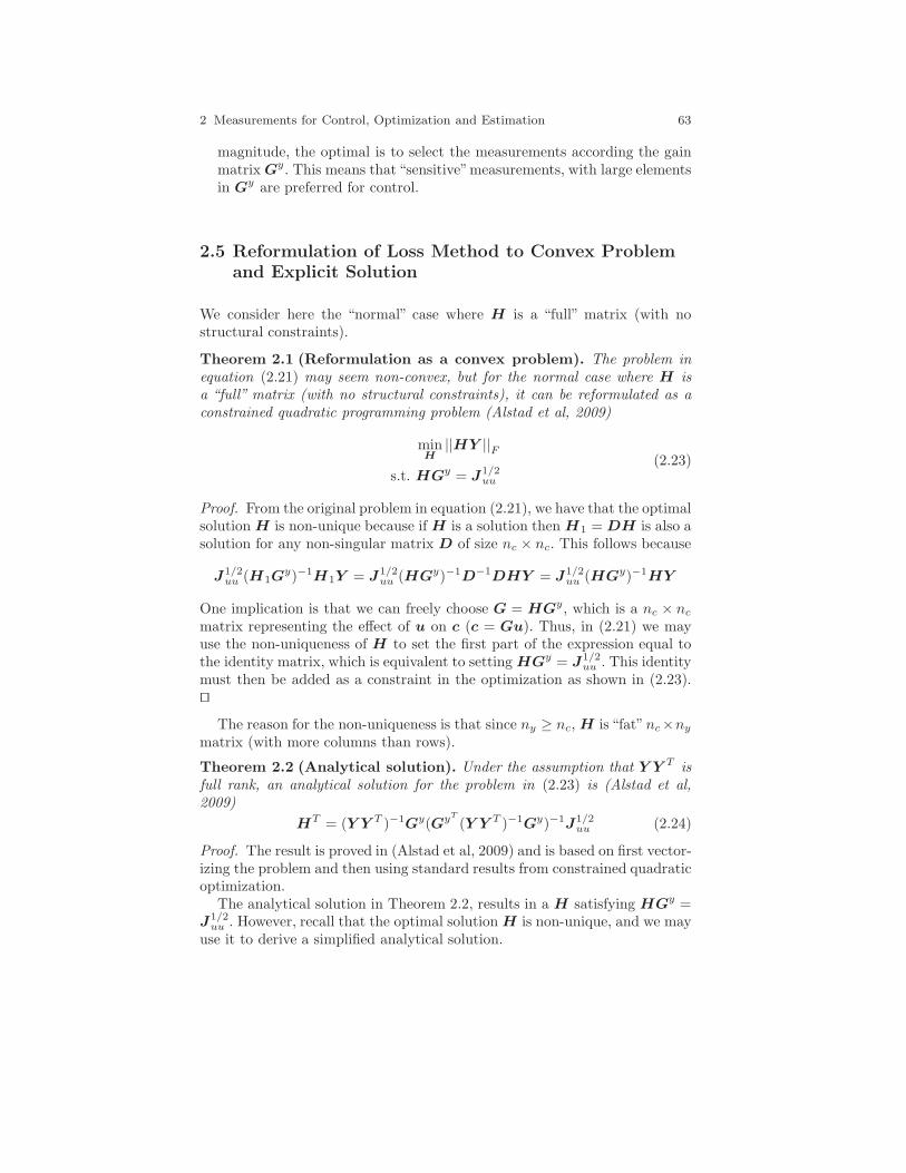
2 Measurements for Control, Optimization and Estimation 63
magnitude, the optimal is to select the measurements according the gainmatrix Gy. This means that “sensitive”measurements, with large elementsin Gy are preferred for control.
2.5 Reformulation of Loss Method to Convex Problemand Explicit Solution
We consider here the “normal” case where H is a “full” matrix (with nostructural constraints).
Theorem 2.1 (Reformulation as a convex problem). The problem inequation (2.21) may seem non-convex, but for the normal case where H isa “full” matrix (with no structural constraints), it can be reformulated as aconstrained quadratic programming problem (Alstad et al, 2009)
minH
||HY ||Fs.t. HGy = J1/2
uu
(2.23)
Proof. From the original problem in equation (2.21), we have that the optimalsolution H is non-unique because if H is a solution then H1 = DH is also asolution for any non-singular matrix D of size nc × nc. This follows because
J1/2uu (H1G
y)−1H1Y = J1/2uu (HGy)−1D−1DHY = J1/2
uu (HGy)−1HY
One implication is that we can freely choose G = HGy, which is a nc × nc
matrix representing the effect of u on c (c = Gu). Thus, in (2.21) we mayuse the non-uniqueness of H to set the first part of the expression equal tothe identity matrix, which is equivalent to setting HGy = J1/2
uu . This identitymust then be added as a constraint in the optimization as shown in (2.23).⊓⊔
The reason for the non-uniqueness is that since ny ≥ nc, H is “fat”nc×ny
matrix (with more columns than rows).
Theorem 2.2 (Analytical solution). Under the assumption that Y Y T isfull rank, an analytical solution for the problem in (2.23) is (Alstad et al,2009)
HT = (Y Y T )−1Gy(GyT
(Y Y T )−1Gy)−1J1/2uu (2.24)
Proof. The result is proved in (Alstad et al, 2009) and is based on first vector-izing the problem and then using standard results from constrained quadraticoptimization.
The analytical solution in Theorem 2.2, results in a H satisfying HGy =J1/2
uu . However, recall that the optimal solution H is non-unique, and we mayuse it to derive a simplified analytical solution.
64 Sigurd Skogestad and Ramprasad Yelchuru and Johannes Jaschke
Theorem 2.3 (Simplified analytical solution). Under the assumptionthat Y Y T is full rank, another analytical solution for the problem in (2.23)is
HT = (Y Y T )−1Gy (2.25)
Proof. This follows trivially from Theorem 2.2, since if HT is a solution then
so is HT1 = HTD and we simply select D = (GyT
(Y Y T )−1Gy)−1J1/2uu =
J−1/2uu GyT
(Y Y T )−1Gy, which is a nc × nc matrix. ⊓⊔Note that the analytical expressions in Theorems 2.2 and 2.3 require Y Y T
to be full rank. This implies that they generally do not apply to the case withno measurement error, W ny = 0, but otherwise they apply for any numberof measurements. One exception (but not so common in practice), when theanalytical expressions for H do apply also for W y = 0, is when ny ≤ nd,
because Y Y T then remains full rank.
Corollary 2.1 (Important insight). Theorem 2.3 gives the very importantinsight that Juu is not needed for finding the optimal H, provided we havethe normal case where H can be any nc × ny matrix.
This means that in (2.21) we can replace J1/2uu by any non-singular matrix,
and still get an optimal H. This can greatly simplify practical calculations,because Juu may be difficult to obtain numerically because it involves thesecond derivative. On the other hand, we found that F , which enters in Y , isrelatively straightforward to obtain numerically. Although Juu is not neededfor finding the optimal H, it would be required for finding a numerical valuefor the loss.
The analytical solutions are useful, in particular for their insights theyyield, but for practical calculations it is usually faster and more robust tocompute the optimal H by solving the convex quadratic optimization prob-lems. In addition, the convex optimization problems do not need the require-ment that Y Y T is non-singular. Based on the insight in Corollary 2.1, thequadratic optimization in Theorem 2.1 (Alstad et al, 2009), can be furtherreformulated to a more general form (Yelchuru and Skogestad, 2010)
Theorem 2.4 (Generalized convex formulation). An optimal H for theproblem in (2.23) is
minH
||HY ||Fs.t. HGy = Q
(2.26)
where Q is any non-singular nc×nc matrix, for example, Q = I, but Q mustbe fixed while minimizing ||HF ||F .Proof. The result follows from Corollary 2.1, but can more generally be de-
rived as follows. The problem in (2.23) is to minimize
∥∥∥∥∥∥(J1/2
uu (HGy)−1
︸ ︷︷ ︸X
HY )
∥∥∥∥∥∥F
.
2 Measurements for Control, Optimization and Estimation 65
The reason why we can omit the nc × nc matrix X, is that if H is an opti-mal solution then so is H1 = DH where D is any nonsingular nc × nc (seeproof of Theorem 2.1). However, note that the matrix X, or equivalently thematrix Q, must be fixed during the optimization, so it needs to be added asa constraint. ⊓⊔
The fact that Q can be chosen freely (Theorem 2.4) can be useful fornumerical reasons, or finding improved bounds for cases with constraints onH (see below).
Once we have found an optimal H using any of the Theorems above,we can use the non-uniqueness of optimal H to find another H1 = DH
with desired property or structure. For example, one can select D such thatG = HGy = I. Alternatively, one can specify selected elements in H1, forexample, H1 = [I K]. In the latter case, write H = [H lHr] and assumeH l is full rank, then H1 = [I K] = [DH l DHr], and we find db = H−1
l
and K = H−1l Hr.
Required information
To find the optimal “full”H using the loss method we need four pieces of in-formation. First, for the measurements we need the optimal disturbance sen-sitivity (F ) and input sensitivity (Gy). These are obtained from the model.Next, we must specify the disturbance magnitudes (Wd) and the noise magni-tudes (Wny ). The matrix Juu is not needed except when there are structuralconstraints, as discussed in the next section.
Note that changes (disturbances) in the prices (parameters) in the costfunction do not change the optimal H, based on the assumption that we stillhave a quadratic optimization problem with constant weights. However, asgiven in (2.22) the setpoint for c needs to be adjusted, cs = HF pp and forthis we need for the measurements the optimal price sensitivity (F p) whichcan be obtained from the model.
2.6 Structural Constraints on H
In the previous section we considered the normal case where H may be any“full” matrix. In terms of selecting controlled variables, c = Hy, this meansthat any combination of measurements are allowed. However, in practice theremay be constraints on H, for example, one wants to use a subset of themeasurements or one want to use a decentralized structure for H .
We will consider the following special cases
Case 1. No restrictions on H. This is the case already considered whereTheorems 2.1– 2.4 hold.
66 Sigurd Skogestad and Ramprasad Yelchuru and Johannes Jaschke
Note that key for deriving Theorems 2.1– 2.4 was that if H is a solutionthen so is H1 = DH where D is any non-singular matrix.
Case 2. H contains a subset of the measurements but is otherwise full.Theorems 2.1– 2.4 hold also in this case.The reason is that H1 = DH will have the same structure as H forany nonsingular D. This is because if H has columns equal to zero, thenthese columns will remain zero in DH even if D is “full”. For example, if
H =
[0 x 0 x x
0 x 0 x x
]then we can still allow a full D =
[x x
x x
](where x is
any number) and keep the structure of H in H1 = DH .Case 3. H contains measurements from disjoint set, so H has a block
diagonal (decentralized) structure. Theorems 2.1– 2.4 do not hold in thiscase.The reason is that for H1 = DH to have the same structure, D must
have a structure similar to H . For example, let H =
[x x x 0 00 0 0 x x
]then
D =
[x 00 x
](where x is any number) and if H =
[x x x x x
0 0 0 x x
]then
D =
[x x
0 x
].
Thus, for case 3 we do not have a convex problem formulation, that is, weneed to solve the nonconvex problem in (2.21) (with additional constraintson the structure of H). This is not surprising as decentralized control isgenerally a nonconvex problem. Nevertheless, Theorems 2.1 and 2.4, withadditional constraints on the structure of H , give convex optimizationproblems that provide upper bounds on the optimal H for case 3. Inparticular, in Theorem 2.4 4 we may make use of the extra degree offreedom provided by the matrix Q (Yelchuru and Skogestad, 2010).Also note that, as opposed to cases 1 and 2, Juu is needed to find theoptimal solution for case 3. This may seem a bit surprising.
Case 4. Decentralized control using single measurements, that is nys = nc
where nys is the number of selected measurements). Theorems 2.1– 2.4hold also in this case.This is a special case of case 3 where we use the fewest number of measure-ments. This case is different from case 2 in that H is a diagonal matrix.The reason why Theorems 2.1– 2.4 hold in this case, is that we can stillkeep D full because the “non-zero” part of H is square and we can tochange it to anything, so we can treat it a special case of “full H”.
2.7 Some Special Cases: Nullspace Method andMaximum Gain Rule
The general optimization problem is
2 Measurements for Control, Optimization and Estimation 67
minH
∣∣∣∣∣∣J1/2
uu (HGy)−1HY )∣∣∣∣∣∣F
(2.27)
where Y = [FW dW ny ]. The objective is to find the nonsquare nc × ny
matrix H (note that nu = nc). We will here consider some special casesof this problem, which historically were developed before the convex andanalytical solutions presented above.
2.7.1 No Measurement Noise: Nullspace Method (“fullH”)
For the special case with no measurement noise, W ny = 0, and with more(independent) measurements than (independent) inputs and disturbances,ny ≥ nu + nd, it is possible to find H such that
HF = 0 (2.28)
that is, the loss is zero. This is called the “nullspace method” (Alstad andSkogestad, 2007) because H is in the nullspace of F . In this case, Gy andW d do not matter for finding the optimal H .
The nullspace method is very simple and has been found to be very usefulin applications. Since the nullspace method neglects the effect of measurementerror, it is important to use preselect a subset of the measurements that areexpected to be insensitive to measurement errors.
Also, one cannot include too many disturbances, because otherwise onecannot satisfy the requirement ny ≥ nu + nd.
One limitation with the analytical formulas in (2.24) and (2.25) is thatthey do not give the nullspace method as a special case. This is becauseY = [FW d Wny ] at most has rank nd when W ny = 0. Thus, the ny × ny
matrix Y Y T at most has rank nd and is not invertible because this wouldrequire the rank to be ny. However, the convex optimization problems inTheorems 2.1 and 2.4 do give the nullspace method as a special case.
Comment: In general, with measurement noise included or with few mea-surements (so ny < nu + nd), it is not possible to make HY zero.
Explicit Expression for H for Nullspace Method
The following explicit expression applies for H (Alstad and Skogestad, 2007):
H = [JuuJud](Gy)−1 (2.29)
Proof. Here is a proof which is much simpler than that given in (Alstad andSkogestad, 2007): Want to find c = Hy with zero loss.
68 Sigurd Skogestad and Ramprasad Yelchuru and Johannes Jaschke
1. Measurement relationship: y = Gy[u
d
]. Inverting this:
[u
d
]= (G
y)−1y (2.30)
2. Optimality condition (NCO):
Ju = 0 (2.31)
3. First-order expansion of gradient:
Ju = J∗u + J∗
uuu+ J∗udd = [J∗
uu J∗ud]
[u
d
]
where we use Ju∗ = 0.
4. (2.30) and (2.31) then give: [Juu Jud]G−1
y y = 0 and it follows that
H = [Juu Jud](Gy)−1. ⊓⊔
2.7.2 No Disturbances
The case with no disturbances has limited practical significance, but is nev-ertheless and interesting limiting cases.
We assume there are no disturbances, W d = 0, and we scale the measure-ments y so that they all have unity measurement noise, W ny = I. From theanalytical expression (2.25), we then have that an optimal solution is
HT = Gy (2.32)
This gives the important insight that we prefer sensitive measurements.
2.7.3 An Approximate Analysis Method for theGeneral Case: “Maximum Gain Rule”
The maximum gain rule is an approximate analysis method for a given H .If we want to compare (analyze) alternative choices for H , for example, al-ternative choices of individual measurements, then the “maximum gain rule”is effective and gives considerable insight. The maximum gain rule has alsobeen used to find “optimal” H, especially for the case where one wants tocontrol individual measurements, and Yu and Kariwala have devised efficientbranch and bound methods for solving this problem.
2 Measurements for Control, Optimization and Estimation 69
In the “maximum gain rule” one considers the scaled gain matrix G =HGy from u to c. To derive the maximum gain rule, we return to the lossexpression
J =1
2zTz
wherez = J1/2
uu (u− uopt) = J1/2uu G−1(c− copt)
c− copt = H(Fd+ ny)
G = HGy
Here, c − copt may be viewed as the “optimal” (or expected) variation inthe selected variables, c = Hy, caused by disturbances and measurementnoise. The magnitude of c − copt = HFd + Hny is obtained by addingthe magnitude of the contributions from HFd and Hny, and we assumein the following that c − copt = W cc
′ where W c is a diagonal matrix forthe expected optimal variation (“optimal span”) in c and we assume that all
||c′||2 ≤ 1 are allowed. c−copt translates into changes in the inputs (u−uopt)
by the transformation u = G−1c and to a loss through the matrix J1/2uu . We
want (u−uopt) small, so we want the norm of G−1 small. More specifically,the largest (worst-case) value of ||z||2 for any allowed ||c′||2 ≤ 1 is equal to
σ(J1/2uu G−1W c), and we want this as small as possible. From singular value
properties we have that the σ(A−1) = 1/σ(A), that is we want to maximize
smin(W−1c GJ−1/2
uu ).We have then derived the maximum gain rule: Under the assumption
that ||c′||2 ≤ 1 , the worst-case loss is given by Lmax = 12
1σ2(Gs)
where
Gs = S1GS2 (2.33)
andS1 = W−1
c = diag(1/|ci − copt,i|)
S2 = J−1/2uu
Note that S1 includes the sum of the optimal variation (as given by the F -matrix) and the expected measurement error. Thus, to minimize the loss weshould select c = Gu with a large minimum singular value of the scaled gainmatrix Gs.
The only “non-exact”step in deriving this rule comes from the assumptionthat all ||c′||2 ≤ 1 are allowed, which means that we neglect some of thevariations in (c−copt) that are correlated. Nevertheless, since the presence ofmeasurement noise means that there is always some uncorrelated variation,at least if we consider individual measurements, c = y, this implies that wecan safely exclude candidate c’s with a small gain, that is, with a small valueof σ(Gs).
70 Sigurd Skogestad and Ramprasad Yelchuru and Johannes Jaschke
Note that Juu enters into the maximum gain rule, whereas it is actually notrequired when H is the optimal full matrix, see (2.26). However, in generalJuu must be included, see case 3 in the discussion following (2.26).
• Do we need the maximum gain rule?
One can analyze the loss with alternatives choices for c using the “exact localmethod”, so why do we need the maximum gain rule? The motivation forusing the maximum gain rule is at least threefold
1. It is simpler to compute.2. It given insight, in particular that we want to control “sensitive” variables
with a large scaled gain: Select variables c where the “optimal variation”(c − copt) (from disturbances, and including measurement noise) is smallcompared to the “achievable variation”(c = Gu) (from inputs).
3. The scaled gain matrix is Gs = S1GS2. Here, the gain matrix G is ob-tained by linearizing in a single operating point. To find the “scaling”matrices S1 and S2 we need to reoptimize for the disturbances (to findc − copt needed for S1) and to find the second derivative with respect to
the inputs (to find S2 = J−1/2uu ), which can be rather involved calculations.
If this information missing, then one may often get good results by esti-mating the optimal variations to find S1 (for example, based on operatingdata) and by setting S2 = I (one should in this case scale the inputs sothat their expected effect on the cost is similar).
This maximum gain rule has also proven to work surprisingly well onmany applications. Nevertheless, if one has data for the optimal sensitivity(F ), then our recommendation is to use the “exact local method” instead ofthe maximum gain rule. This is because one can analyze alternative choicesfor c (and H) more exactly by computing the norm (Frobenius norm or max.
singular value) of M =[J1/2
uu (HGy)−1HY]. Kariwala and Cao (2009) have
derived efficient branch and bound algorithms for finding the measurementchoice (optimal structured H) that minimize either the norm of M as wellas the scaled gain, σ(Gs). Although the computation times for minimizingthe latter are somewhat lower, the benefit is not sufficiently large to justifyusing the maximum gain rule, provided we have the necessary informationavailable for the first method.
2.8 Indirect Control and Estimation of Primary Variable
These two problems are very similar, and can be written as a special case ofthe loss method, involving the same matrices.
2 Measurements for Control, Optimization and Estimation 71
2.8.1 Indirect Control of y1
The objective is to keep the primary output y1 close to its setpoint, so thecost function is
J = (y1 − y1,s)2
However, y1 is not measured, but we have to use some other measurementsy. Thus, we want to achieve indirect control of y1 by keeping c = Hy at agiven setpoint.
To find the optimal “full” H using the loss method we need four piecesof information; F , Gy,Wd,Wny . In our case, the optimal sensitivity is F =(dyopt/dd) = (dy/dd)y1
It may be obtained by simulations where we keepy1 constant for the various disturbances. Instead of using simulations, wemay write y1 = G1u + Gd1d, and then (Hori et al, 2005) Juu = Gt
1G1,Jud = GT
1 Gd1, F = (−GyJ−1
uuJud +Gyd) = (−GyG−1
1 Gd1+G
yd).
In addition, we need to handle setpoint changes for the primary variable,y1,s, which requires changes in the setpoint for c. Note that y1,s only affectsthe cost function and may be viewed as a price variable p, so from (2.22)the required change in the setpoint is ∆cs = HFp∆y1,s, where Fp may beobtained from the model (exercise: derive the expression!).
2.8.2 Indirect Control of y1 Based on Estimator
Note that we still have not used the available degrees of freedom in H . Tosimplify the setpoint adjustment, we may use the degrees of freedom in H
to make HFp = I, or equivalently, c = y1. This means that c should bean estimate of y1. Note that y1 = G1u and c = HG1u (setting d = 0 forsimplicity). These two gains need to be identical, so we use the extra degreesof freedom in H to make
HGy = G1 (2.34)
It is then easy to include changes in setpoint; we just control c at y1,s.
Some comments on this estimator
• What kind of estimator is this? If we look at the problem formulation, thenwe see that it is be the optimal estimator in the following sense: When wecontrol y1 at the estimate (using the unconstrained degrees of freedom)then this minimizes the deviation from the given value (setpoint), for theexpected range of disturbances and measurement noise.
• For practical purposes, when obtaining the model, it may be smart to letthe primary outputs be the degrees of freedom, u = y1 that is, to use
72 Sigurd Skogestad and Ramprasad Yelchuru and Johannes Jaschke
“closed-loop data” (this may seem strange, but it is OK). Then we haveG1 = I.
2.9 Estimator for y1 Based on Data
The idea is to use the same approach as for the previous problem, but usingdata instead of a model. The objective is to estimate y1 based on measure-ments y (which we from now on will call x to follow statistics notation). Thatis, we want to find
y1 = Hx
(where x = y). The available information is given by the data Y all =[Y 1;X]. Note that the data must first be centered.
To use our method, we first need to know the expected optimal variationY . Here “optimal” means that y1 is constant. In addition, we also need toobtain Gy and G1 from the data. This means that the data must contain“non-optimal” variations in u, and not only contain optimal data where u =uopt(d).
Comment: The setup is the same as for the previous problem, expect thatit is not clear how noise in y1 can be included. It is a bit similar to “imple-mentation error”which has been neglected since we assumed integral action.
2.9.1 Data Approach 1
Here we assume that Y all is obtained from two different sources of data.
1. “Optimal” data with constant y1(X = Y opt): This is closed-loop data fory with y1 constant for various disturbances (d) and also with noise. Itshould be representative data for the expected operation. This directlygives the matrix Y = Y opt (including the weights) needed in (2.26).
2. “Non-optimal” data with constant d: This is data for x and y1 collectedwith varying u. From this data we directly obtainGy and G1. By selectingu = y1, one may also here used closed-loop data (but with y1 varying), inthis case G1 = I.
3. Find optimal H using (2.26) with HGy = I.
2.9.2 Data Approach 2: Loss Regression
More generally, we do not have separate “optimal” and “non-optimal” data.Instead, we have combined data Y all where y1 and x vary simultaneously.
2 Measurements for Control, Optimization and Estimation 73
Note that we here use the notation from statistics/chemometrics and call themeasurements y for x.
We can then do a two-step procedure. In the first step, we “split up” thedata Y all data to find G1, G
y and Y opt, and in step 2 we proceed as“normal”to find the optimal H .
Step 1A. We rearrange the data Y all such that the y1 values are in thefirst rows, and the x = y-measurements are in the rest (called X),
Y all = [Y 1;X]
Step 1B. We now want to separate the data into “optimal” and “nonop-timal” data. The data can generally be transformed by multiplying by a(real) unitary matrix V , because ||[HY all]|| = ||[HY allV ]|| for the 2-norm. Thus, we can use the SVD of
Y 1 = U1S1VT1
to transform the data to (“split up the data”)
Y allV 1 =
[G1 0Gy Xopt
]
Now, we have G1, Gy and Y = Xopt and can proceed as normal using
our derived formulas, see earlier.Step 2. Find the optimal H by solving the convex optimization in (2.26)
with Y = Xopt and the constraint HGy = G1.
% Loss method
% step 1A
Yall = [Y1; X];
% step 1B
[u,s,v]=svd(Y1);
Yall1 = Yall*v;
[r1,c1]=size(Yall);
[r2,c2]=size(Y1);
ny=r2;
G1=Yall1(1:ny,1:ny);
Gy=Yall1(ny+1:r1,1:ny);
Xopt = Yall1(ny+1:r1,ny+1:c1);
% step 2,
%Hopt = (pinv(Xopt*Xopt’)*Gy)’; %analytical expression
[Hopt,loss]=soc_avg(Gy,Xopt);
D=Hopt*Gy*inv(G1);
Hoptloss=inv(D)*Hopt;
74 Sigurd Skogestad and Ramprasad Yelchuru and Johannes Jaschke
Comments
• Alternatively in step 2, provided Y Y T has full rank, we may use theanalytical expression HT = (Y Y T )−1Gy in (2.25) and then “rescale”Hto get a new H1 = DH which satisfies H1G
y = G1, which gives H1 =G1(HGy)−1H . If Y Y T does not have full tank one may use some pseudoinverse (similar to PCR). This adds degrees of freedom to the method. Ithas not been tested out but some preliminary results are promising.
• The method seems a bit similar to PLS in that we use the data for y1 toaffect the x-data (we get Xopt from X by using the SVD of Y 1, and alsouse Gy when minimizing HXopt.
2.9.2.1 Modification for Case with Too Few Experiments (e.g.Spectroscopic Data)
If we start with a model, then the data matrix Y = [FW d Wny ] is a “fat”matrix; this is clear since the noise magnitude matrix Wny is a square matrix(usually diagonal). Thus, there exists no matrix H such that HY = 0.
However, if we start with data and have many measurements (e.g., spec-troscopic data), then Y = Xopt is likely a thin matrix, and there will exist an(or actually, infinitely many) H such that HY = 0. Since the experimentaldata Y contains measurement noise, this means that H is “fitting” the noise.The proposed method will then be very similar to least squares, althoughthe constraint HGy = G1 can make it different (as seen from the numericalexamples below).
Extra step 1C. To fix this up, one may add“artificial”measurement noiseto get a better representation of the actual measurement noise. Since therewill always be some independent noise for each measurement, it is suggestedto add a diagonal matrix Wny to the original data
Xextended = [XoptWny ]
where Xopt was found in Step 1B above.The problem is now to choose Wny . One approach is to estimate it from
the data using a preprocessing step. For example, one may do some prelimi-nary regression and from this obtain an estimate of the noise.
A very simple approach, which is tested on some applications below, is toassume that the measurements have been scaled (for example, by the normof the variation in each measurement), such that they have similar expectedmagnitudes. Thus, we use Wny = wnY where wn is a scalar.
noise = wn*eye(rx);
Xoptnoise = [Xopt noise];
[Hopt,loss]=soc_avg(Gy,Xoptnoise);
% etc......
2 Measurements for Control, Optimization and Estimation 75
wn is a tuning parameter but a systematic approach is the following: Plotthe singular values of Xopt and select wn such that the singular values ofXextended follow the same trend.
2.9.3 Modification: Smoothening of Data
The loss regression method is based on the loss method where it is assumedthat a model is available. When we are using data, then the model has tobe extracted first (step 1), and this step of the method is not based on arigorous approach to the final objective, which is to use the model for futurepredictions.
Therefore, it is likely that this step may be improved, One possible modi-fications is suggested next, although it seems from the later numerical teststhat it actually may have no effect.
2.9.3.1 Smoothening of y1
The above procedure (including step 1) assumes that all the noise is in thex = y. One way of dealing noise in y1 is to run through the procedure twice.
First, we go through the procedure (steps 1 and 2) and find the optimalH0.
Next, we go through the procedure again, but with a modified step 1Awhere use H0 to estimate the smoothened (fitted) values of y1 that corre-spond to the measured X,
Y smooth1 = H0X
and then we use this smoothened data in the other steps,
Y all = [Y smooth1 ;X]
Y1smooth = Hoptloss*X;
% then redo step 1 and 2
Yallsmooth = [Y1smooth; X];
[u,s,v]=svd(Y1smooth);
% etc....
However, from the numerical examples this smoothening has no effect onthe results, which in some sense is good, but on the other hand it does notoffer any extra degrees of freedom.
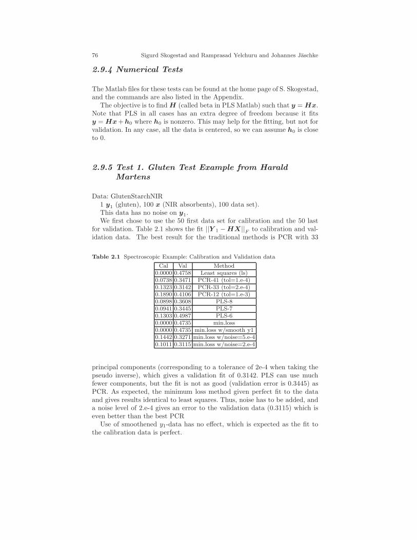
76 Sigurd Skogestad and Ramprasad Yelchuru and Johannes Jaschke
2.9.4 Numerical Tests
The Matlab files for these tests can be found at the home page of S. Skogestad,and the commands are also listed in the Appendix.
The objective is to find H (called beta in PLS Matlab) such that y = Hx.Note that PLS in all cases has an extra degree of freedom because it fitsy = Hx+h0 where h0 is nonzero. This may help for the fitting, but not forvalidation. In any case, all the data is centered, so we can assume h0 is closeto 0.
2.9.5 Test 1. Gluten Test Example from HaraldMartens
Data: GlutenStarchNIR1 y1 (gluten), 100 x (NIR absorbents), 100 data set).This data has no noise on y1.We first chose to use the 50 first data set for calibration and the 50 last
for validation. Table 2.1 shows the fit ||Y 1 −HX||F to calibration and val-idation data. The best result for the traditional methods is PCR with 33
Table 2.1 Spectroscopic Example: Calibration and Validation data
Cal Val Method0.0000 0.4758 Least squares (ls)0.0738 0.3471 PCR-41 (tol=1.e-4)0.1323 0.3142 PCR-33 (tol=2.e-4)0.1890 0.4106 PCR-12 (tol=1.e-3)0.0898 0.3608 PLS-80.0941 0.3445 PLS-70.1303 0.4987 PLS-60.0000 0.4735 min.loss0.0000 0.4735 min.loss w/smooth y10.1442 0.3271 min.loss w/noise=5.e-40.1011 0.3115 min.loss w/noise=2.e-4
principal components (corresponding to a tolerance of 2e-4 when taking thepseudo inverse), which gives a validation fit of 0.3142. PLS can use muchfewer components, but the fit is not as good (validation error is 0.3445) asPCR. As expected, the minimum loss method given perfect fit to the dataand gives results identical to least squares. Thus, noise has to be added, anda noise level of 2.e-4 gives an error to the validation data (0.3115) which iseven better than the best PCR
Use of smoothened y1-data has no effect, which is expected as the fit tothe calibration data is perfect.
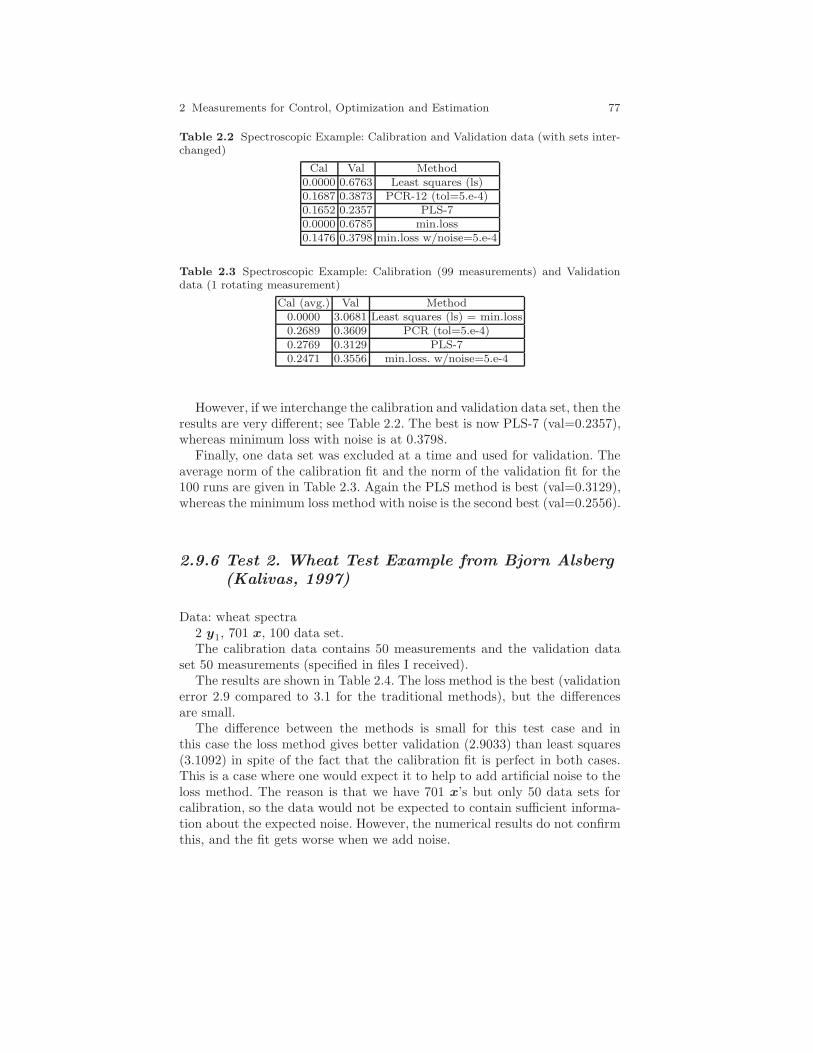
2 Measurements for Control, Optimization and Estimation 77
Table 2.2 Spectroscopic Example: Calibration and Validation data (with sets inter-changed)
Cal Val Method0.0000 0.6763 Least squares (ls)0.1687 0.3873 PCR-12 (tol=5.e-4)0.1652 0.2357 PLS-70.0000 0.6785 min.loss0.1476 0.3798 min.loss w/noise=5.e-4
Table 2.3 Spectroscopic Example: Calibration (99 measurements) and Validationdata (1 rotating measurement)
Cal (avg.) Val Method0.0000 3.0681 Least squares (ls) = min.loss0.2689 0.3609 PCR (tol=5.e-4)0.2769 0.3129 PLS-70.2471 0.3556 min.loss. w/noise=5.e-4
However, if we interchange the calibration and validation data set, then theresults are very different; see Table 2.2. The best is now PLS-7 (val=0.2357),whereas minimum loss with noise is at 0.3798.
Finally, one data set was excluded at a time and used for validation. Theaverage norm of the calibration fit and the norm of the validation fit for the100 runs are given in Table 2.3. Again the PLS method is best (val=0.3129),whereas the minimum loss method with noise is the second best (val=0.2556).
2.9.6 Test 2. Wheat Test Example from Bjorn Alsberg(Kalivas, 1997)
Data: wheat spectra2 y1, 701 x, 100 data set.The calibration data contains 50 measurements and the validation data
set 50 measurements (specified in files I received).The results are shown in Table 2.4. The loss method is the best (validation
error 2.9 compared to 3.1 for the traditional methods), but the differencesare small.
The difference between the methods is small for this test case and inthis case the loss method gives better validation (2.9033) than least squares(3.1092) in spite of the fact that the calibration fit is perfect in both cases.This is a case where one would expect it to help to add artificial noise to theloss method. The reason is that we have 701 x’s but only 50 data sets forcalibration, so the data would not be expected to contain sufficient informa-tion about the expected noise. However, the numerical results do not confirmthis, and the fit gets worse when we add noise.
78 Sigurd Skogestad and Ramprasad Yelchuru and Johannes Jaschke
Y 1 contains both the two y-variables (water and protein); presumablybetter fit can be obtained by fitting one at a time.
Table showing the fit ||Y 1 −HX||F to calibration and validation data:
Table 2.4 Wheat Spectra Calibration and Validation data
Cal. Val. Method0.0000 3.1092 least squares (= PCR -50)0.3136 3.0871 PCR-47 (tol=1.1 e-3)0.0052 3.1052 PLS-350.0000 2.9033 min.loss0.0000 2.9033 min.loss + noise=1.e-80.0069 3.1099 min.loss + noise=1.e-4
Again, smoothening of y1 has no effect, which again is not surprising sincethe fit was perfect.
2.9.7 Test 3. Our Own Example
The data contains 2 y1, 7 x, 2 d.
G1 =
[1 00 1
]Gd1
=
[0 00 0
]gy1
= [0.2034563] gy2= [00.213489] Gy =
[gTy1, gTy2
] gd1= [004568− 9] gd2
= [00− 3− 55918] Gyd= [gTd1
; gTd2]
8 (or 32) noisy data set generated from ideal data [GyGyd] (4 data sets)
with 2 (or 8) different noise sets to get a total of 8 data sets. We here generatethe data by adding noise to data from a model (“calibration set”) and the“validation set” is the noise-free data. To center the data I used oppositesign when the data was “repeated”. The noise was generated using randncommand in Matlab.
It was found that when tested on a single example then almost any of themethods could be the winner. To avoid this effect, the comparison was runmany times (with different random noise).
Table 2.5 shows the average value of ||Y 1 −HX||F for 8 data sets afterrunning 250 times. The best method is PCR (val=0.4931), PLS with 4 com-ponents (val=0.5137) is the best PLS. This is not surprising since we knowthat the data contains 4 directions. The new loss method is not doing so wellin this case (val=1.055), which is not so surprising since with only 8 datasets there is limited information about the noise. Note that it is even worsethan least squares (val=0.9985). As expected, the improvement by addingnoise was significant (val=0.5850), but it is still not quite as good as PCRand PLS.
Surprisingly, smoothening of y1 had absolutely no effect in this case, evenwhen I added noise on the y1-data (results not shown).

2 Measurements for Control, Optimization and Estimation 79
Table 2.5 Our own example: 8 data sets in each run (average of 500 runs)
w/noise(cal) no noise(val) Method0.2934 0.9985 LS (=PCR-8)0.5496 0.4931 PCR (tol=1, most cases PCR-5)0.5102 0.5137 PLS-40.3150 1.0552 loss method (no noise)0.3150 1.0552 loss method (smooth y1)0.4205 0.5850 loss method (noise=0.5)
Now, to show that the loss method does better when there is more data,Table 2.6 shows the average value of ||Y 1 −HX||F for 32 data sets afterrunning 300 times.
Table 2.6 Our own example: 32 data sets in each run (average of 300 runs)
w/noise(cal) no noise(val) Method1.4826 0.3560 LS (=PCR-8)1.4970 0.3560 PCR (most cases PCR-6)1.5256 0.3698 PLS-41.7700 0.2690 loss method (no noise)1.7700 0.2690 loss method (smooth y1)1.7703 0.2687 loss method (noise=0.5)
The loss method is the winner (val = 0.269) in spite of the fact that it hasno “tuning” parameters.
Here there is little effect of adding artificial noise with the loss method,presumable because we have enough data.
2.9.8 Comparison with Normal Least Squares
Normal least square solution. Problem: Find H such that the magnitude of||Y 1 −HY ||2 is minimized for the given set of data for Y 1 and Y .
Solution: H = Y 1pinv(Y ). This minimizes ||Y 1 −HY ||2 and, for caseswhere this H is not unique, minimizes ||H ||2.
This is the same as finding H to minimize ||[I H ]Y all||, which we knowis not the optimal solution
Proof. The data matrix is Y all = [Y 1;Y ] Assume that we seek Hall tominimize ||HallY all||2. We have degrees of freedom in Hall, so we set Hall =[I −H]. Then we want to minimize ||Hall[Y 1;Y ]||2 = ||−Y 1 +HY || thebest solution is given by the pseudo inverse, H = Y 1pinv(Y ) which is theusual least square solution. ⊓⊔
So why is least squares not optimal?
80 Sigurd Skogestad and Ramprasad Yelchuru and Johannes Jaschke
The “problem” (objectives function) for normal least squares is to get thebest match of the available data, ie., minimize ||Y 1 −HX||, and it does notconsider how the estimate y1 = Hx is going to be used in the future.
So why is the loss approach expected to be better?In the loss approach, the problem is:Given that y1 = Hx, find an optimal H such that the average magnitude
of ||y1 − y1||2 is minimized for the expected future ds and nys (which areassumed 2-norm bounded).
Here, we use the data to obtain Y = Y opt, Gy and G1 (step 1). This step
may possibly be improved but it seems reasonable.The main advantage is that in step 2, we obtain the estimate y1 = Hy that
will work best “on average” for the expected disturbances and measurementnoise (as are indirectly given by the data in Y opt, that is, we consider thefuture use of the estimator and not just fitting of the data).
2.10 Discussion
2.10.1 Gradient Information
How can we use the proposed approach in practice, for example, to find theoptimal policy for a marathon runner. We need to be able to distinguishbetween “optimal data” (Y opt) and “nonoptimal data” to find Gy and G1. Asimple approach is to set y1 = Ju (that is, we want to estimate the gradient).Then we know that optimal data corresponds to y1 = Ju = 0 and we cando exactly as above (Data approach 1 or 2). However, note that this meansthat we need some non-optimal data where we know the value of Ju.
2.10.2 Relationship to NCO tracking
Finally, some ideas related to NCO tracking.The NCO-idea is to set the Gradient= 0. An important difference com-
pared to the proposed loss approach, is that in NCO-tracking one tries tofind an expression for u (“open-loop implementation” similar to deadbeatcontrol).
On the other hand in the loss method (self-optimizing control), we “stop”when we have the expression for the gradient c = Ju. the implementation tofind u that gives Ju = 0 is by feedback control!
From (2.10) and (2.11) we see that we want to minimize (u−uopt) or Ju
(but weighted by Juu). Recall here that in the full-H case, Juu is not needed.Still, it remains unclear if this means that we can just minimize ||Ju||?

2 Measurements for Control, Optimization and Estimation 81
Another problem with NCO idea to “Control gradient to zero” is that thisis not really possible since gradient can not be measured. Thus, it needs to beestimated. For the case with no noise the estimate Ju is same as “nullspacemethod”, so c = Hy = Ju!
For noisy case not so clear, but may as well use c = Hy.
2.11 Appendix
1
2 % This is file matlab-test-cases.m
3 % Load data from C:\Documents and Settings\skoge\My Documents\
MATLAB
4
5 % -------------------------------------------------
6 % Test case 1. Martens data:
7 load GlutenStarchNIR
8 % X: Variablene 13-112 er NIR absorbanser (log(1/T) fra
850-1048 nm).
9 % y1: Variabel 4 er kvantitiv analytt-konsentrasjon (gluten),
10 % Matrix: 100 rows 112 cols: regular MATLAB matrix
11 % VarLabels: 112 rows 17 cols: MATLAB character string
12 % ObjLabels: 100 rows 7 cols: MATLAB character string
13 Yall=Matrix’;
14 XX = Yall(13:112,:);
15 YY = Yall(4,:);
16 X = XX(:,1:50);
17 X0= XX(:,51:100);
18 Y1= YY(:,1:50);
19 Y10=YY(:,51:100);
20
21 % repeated Martens
22 % 100 times where I take out data each time
23 %for nsis=1:98
24 %X = XX(:,[1:nsis nsis+2:100]); X0 = XX(:,nsis+1);
25 %Y1 = YY(:,[1:nsis nsis+2:100]); Y10 = YY(:,nsis+1);
26 % Two end cases are handled separately
27 %nsis=0
28 %X = XX(:,[nsis+2:100]); X0 = XX(:,nsis+1);
29 %Y1 = YY(:,[nsis+2:100]); Y10 = YY(:,nsis+1);
30 %nsis=99
31 %X = XX(:,[1:nsis]); X0 = XX(:,nsis+1);
32 %Y1 = YY(:,[1:nsis]); Y10 = YY(:,nsis+1)
33
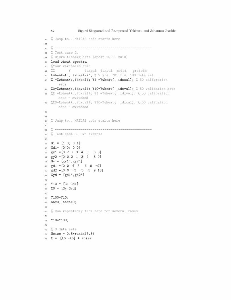
82 Sigurd Skogestad and Ramprasad Yelchuru and Johannes Jaschke
34 % Jump to.. MATLAB code starts here
35
36 % -------------------------------------------------
37 % Test case 2.
38 % Bjørn Alsberg data (epost 15.11 2010)
39 load wheat_spectra
40 %Your variables are:
41 %X Y idxcal idxval moist protein
42 Xwheat=X’; Ywheat=Y’; % 2 y’s, 701 x’s, 100 data set
43 X =Xwheat(:,idxcal); Y1 =Ywheat(:,idxcal); % 50 calibration
sets
44 X0=Xwheat(:,idxval); Y10=Ywheat(:,idxval); % 50 validation sets
45 %X =Xwheat(:,idxval); Y1 =Ywheat(:,idxval); % 50 calibration
sets - switched
46 %X0=Xwheat(:,idxcal); Y10=Ywheat(:,idxcal); % 50 validation
sets - switched
47
48
49 % Jump to.. MATLAB code starts here
50
51 % -------------------------------------------------
52 % Test case 3. Own example
53
54 G1 = [1 0; 0 1]
55 Gd1= [0 0; 0 0]
56 gy1 =[0.2 0 3 4 5 6 3]
57 gy2 =[0 0.2 1 3 4 8 9]
58 Gy = [gy1’,gy2’]
59 gd1 =[0 0 4 5 6 8 -9]
60 gd2 =[0 0 -3 -5 5 9 18]
61 Gyd = [gd1’,gd2’]
62
63 Y10 = [G1 Gd1]
64 X0 = [Gy Gyd]
65
66 Y100=Y10;
67 na=0; aa=a*0;
68
69 % Run repeatedly from here for several cases
70
71 Y10=Y100;
72
73 % 8 data sets
74 Noise = 0.5*randn(7,8)
75 X = [X0 -X0] + Noise
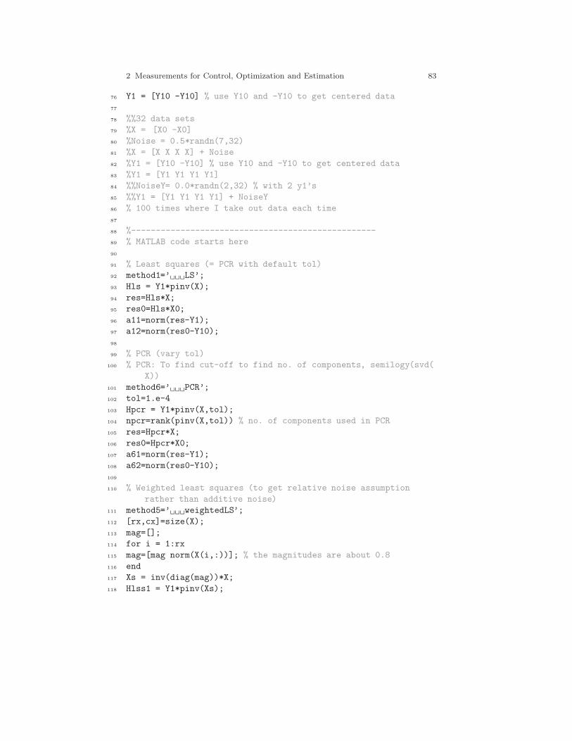
2 Measurements for Control, Optimization and Estimation 83
76 Y1 = [Y10 -Y10] % use Y10 and -Y10 to get centered data
77
78 %%32 data sets
79 %X = [X0 -X0]
80 %Noise = 0.5*randn(7,32)
81 %X = [X X X X] + Noise
82 %Y1 = [Y10 -Y10] % use Y10 and -Y10 to get centered data
83 %Y1 = [Y1 Y1 Y1 Y1]
84 %%NoiseY= 0.0*randn(2,32) % with 2 y1’s
85 %%Y1 = [Y1 Y1 Y1 Y1] + NoiseY
86 % 100 times where I take out data each time
87
88 %--------------------------------------------------
89 % MATLAB code starts here
90
91 % Least squares (= PCR with default tol)
92 method1=’ LS’;
93 Hls = Y1*pinv(X);
94 res=Hls*X;
95 res0=Hls*X0;
96 a11=norm(res-Y1);
97 a12=norm(res0-Y10);
98
99 % PCR (vary tol)
100 % PCR: To find cut-off to find no. of components, semilogy(svd(
X))
101 method6=’ PCR’;
102 tol=1.e-4
103 Hpcr = Y1*pinv(X,tol);
104 npcr=rank(pinv(X,tol)) % no. of components used in PCR
105 res=Hpcr*X;
106 res0=Hpcr*X0;
107 a61=norm(res-Y1);
108 a62=norm(res0-Y10);
109
110 % Weighted least squares (to get relative noise assumption
rather than additive noise)
111 method5=’ weightedLS’;
112 [rx,cx]=size(X);
113 mag=[];
114 for i = 1:rx
115 mag=[mag norm(X(i,:))]; % the magnitudes are about 0.8
116 end
117 Xs = inv(diag(mag))*X;
118 Hlss1 = Y1*pinv(Xs);

84 Sigurd Skogestad and Ramprasad Yelchuru and Johannes Jaschke
119 Hlss = Hlss1*inv(diag(mag));
120 ress=Hlss*X;
121 ress0=Hlss*X0;
122 a51=norm(ress-Y1) ;
123 a52=norm(ress0-Y10) ;
124
125 % pls
126 npls=35
127 %npls=npcr
128 [XL,yl,XS,YS,beta,PCTVAR] = plsregress(X’,Y1’,npls);
129 % Note that PLS has an additional bias/centering parameter.
130 yfit = [ones(size(X’,1),1) X’]*beta;
131 yfit0 = [ones(size(X0’,1),1) X0’]*beta;
132 a71=norm(yfit-Y1’);
133 a72=norm(yfit0-Y10’);
134 method7=’ PLS’;
135
136 % Loss method
137 % step 1
138 Yall = [Y1; X];
139 [u,s,v]=svd(Y1);
140 Yall1 = Yall*v;
141 [r1,c1]=size(Yall);
142 [r2,c2]=size(Y1);
143 ny=r2;
144 G1=Yall1(1:ny,1:ny);
145 Gy=Yall1(ny+1:r1,1:ny);
146 Xopt = Yall1(ny+1:r1,ny+1:c1);
147
148 % step 2,
149 %Hopt = (pinv(Xopt*Xopt’)*Gy)’; %analytical expression
150 [Hopt,loss]=soc_avg(Gy,Xopt);
151 D=Hopt*Gy*inv(G1); %
152 Hopt4=inv(D)*Hopt;
153 resb=Hopt4*X;
154 resb0=Hopt4*X0 ;
155 a41=norm(resb-Y1) ;
156 a42=norm(resb0-Y10) ;
157 method4=’ loss ’;
158
159 % NEW modified loss method for case with noise on Y: redo step
1.
160 % New estimate of Y1.
161 Y1smooth = Hopt4*X;
162 % then redo step 1 and 2

2 Measurements for Control, Optimization and Estimation 85
163 Yallsmooth = [Y1smooth; X];
164 [u,s,v]=svd(Y1smooth);
165 Yallsmooth = Yall*v;
166 G1smooth=Yallsmooth(1:ny,1:ny);
167 Gysmooth=Yallsmooth(ny+1:r1,1:ny);
168 Xsmooth = Yallsmooth(ny+1:r1,ny+1:c1);
169 % step 2
170 [Hopt,loss]=soc_avg(Gysmooth,Xsmooth);
171 D=Hopt*Gysmooth*inv(G1smooth); %
172 Hopt10=inv(D)*Hopt;
173 resa=Hopt10*X;
174 resa0=Hopt10*X0 ;
175 a101=norm(resa-Y1) ;
176 a102=norm(resa0-Y10) ;
177 method10=’ loss w/smooth’;
178
179 % loss method: add artificial noise weights
180 noisemag=2.e-4
181 %noisemag=tol
182 % Noise Alt.1 just additive noise:
183 noise = noisemag*eye(rx);
184 Xoptnoise = [Xopt noise];
185 % Noise Alt2. Add noise proportional to variation in each
output
186 %[rx,cx]=size(Xopt);
187 %mag=[];
188 %for i = 1:rx
189 %mag=[mag norm(Xopt(i,:))]; % the magnitudes are about 0.8
190 %end
191 %noise = noisemag*diag(mag);
192 %Xoptnoise = [Xopt noise];
193
194 % step 2- with artificial noise
195 % semilogy(svd(X))
196 % semilogy(svd([X X0])
197 [Hopt,loss]=soc_avg(Gy,Xoptnoise);
198 D=Hopt*Gy*inv(G1); %
199 Hopt9=inv(D)*Hopt;
200 resb=Hopt9*X;
201 resb0=Hopt9*X0 ;
202 a91=norm(resb-Y1) ;
203 a92=norm(resb0-Y10) ;
204 method9=’ loss w/noise’;
205
206 % Summary of results

86 Sigurd Skogestad and Ramprasad Yelchuru and Johannes Jaschke
207 methods=[method1 method5 method6 method7 method4 method10
method9]
208 a =[a11 a12; a51 a52; a61 a62; a71 a72; ; a41 a42; a101 a102;
a91 a92]’
209
210 % For repeated case 1 and case 3:
211 na=na+1
212 aa=aa+a;
213 aaa=aa/na
214 % For repeated case 1
215 end
Acknowledgements The authors are pleased to acknowledge the financial supportfrom the NIL-I-007-d project and the Norwegian Research Council
References
Alstad V, Skogestad S (2007) Null space method for selecting optimal measurementcombinations as controlled variables. Ind Eng Chem Res 46:846–853
Alstad V, Skogestad S, Hori E (2009) Optimal measurement combinations as con-trolled variables. Journal of Process Control 19(1):138–148
Halvorsen IJ, Skogestad S, Morud JC, Alstad V (2003) Optimal selection of controlledvariables. Ind Eng Chem Res 42
Hori ES, Skogestad S, Alstad V (2005) Perfect steady-state indirect control. Industrial& Engineering Chemistry Research 44(4):863–867
Kariwala V, Cao Y (2009) Bidirectional branch and bound for controlled vaiableselection. part ii: Exact local method for self-optimizing control. Computers andChemical Engineering 33:1402–1414
Kariwala V, Cao Y, Janardhanan S (2008) Local self-optimizing control with averageloss minimization. Ind Eng Chem Res 47:1150–1158
Yelchuru R, Skogestad S (2010) Miqp formulation for optimal controlled variableselection in self optimizing control. In: PSE Asia, 2010. July 25-28, Singapore

2 Measurements for Control, Optimization and Estimation 87
Comments – Remarks

88 Sigurd Skogestad and Ramprasad Yelchuru and Johannes Jaschke
Comments – Remarks

2 Measurements for Control, Optimization and Estimation 89
Comments – Remarks

90 Sigurd Skogestad and Ramprasad Yelchuru and Johannes Jaschke
Comments – Remarks
Chapter 3
Measurement polynomials as controlledvariables – Exercises
Johannes Jaschke and Sigurd Skogestad
Abstract In this chapter we present two exercises for finding controlledvariables, which are polynomials in the measurements. Detailed solutionsand maple source code are included so that the reader can easily follow theprocedure.
3.1 Introduction
To illustrate concepts from described in the textbook, we present some smallproblem and go through the solution step by step. The reader is encouragedto experiment on his own to understand the ideas better.
For solving the CSTR case study, the multires package is required1
3.2 Simple excercise
Exercise 3.1 (Cox 1992). Check whether the two polynomials f1 = 2x2 +3x+ 1 and f2 = 7x2 + x+ 3 have a common root in C.
Solution 3.1. The resultant is the determinant of the Sylvester matrix:
Johannes JaschkeDepartment of Chemical Engineering, NTNU Trondheim, Norway, e-mail: [email protected]
Sigurd SkogestadDepartment of Chemical Engineering e-mail: [email protected]
1 The software can be downloaded at www-sop.inria.fr/galaad/software/multires
91
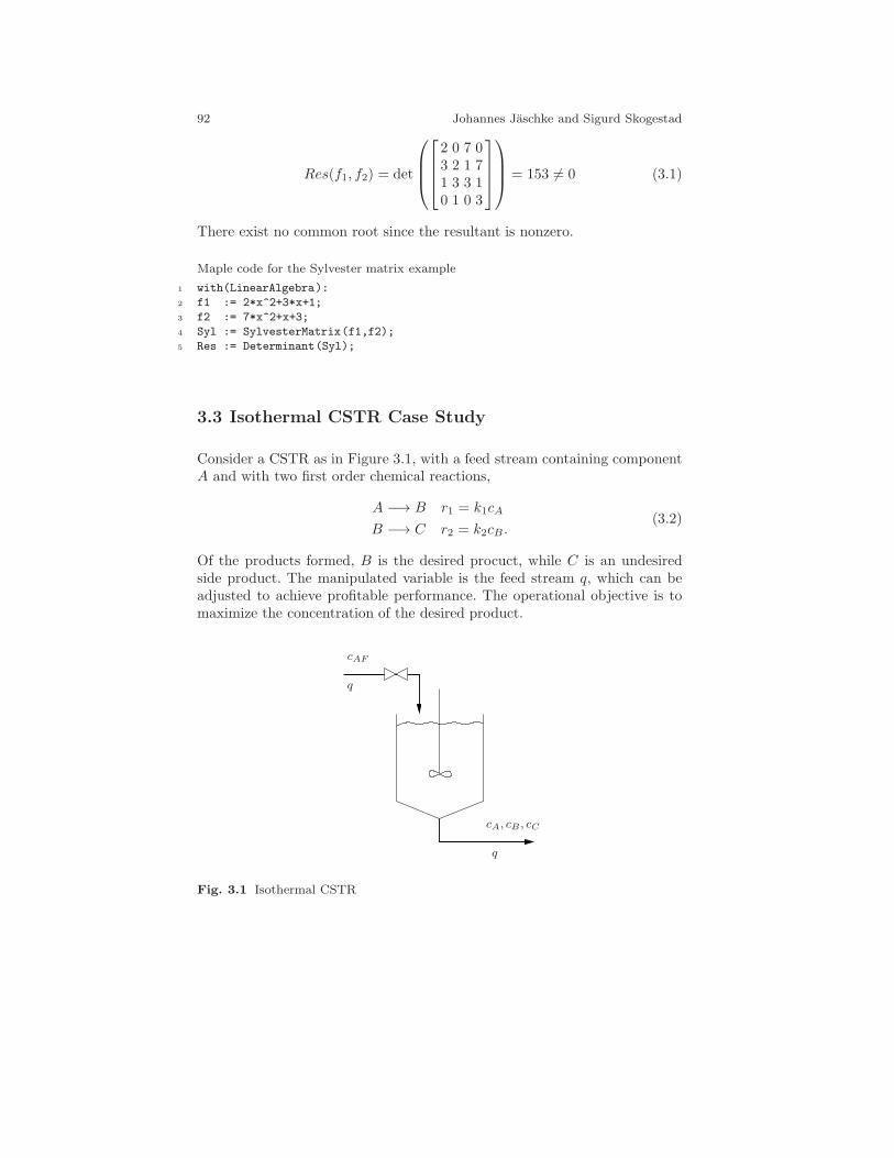
92 Johannes Jaschke and Sigurd Skogestad
Res(f1, f2) = det
2 0 7 03 2 1 71 3 3 10 1 0 3
= 153 6= 0 (3.1)
There exist no common root since the resultant is nonzero.
Maple code for the Sylvester matrix example
1 with(LinearAlgebra):
2 f1 := 2*x^2+3*x+1;
3 f2 := 7*x^2+x+3;
4 Syl := SylvesterMatrix(f1,f2);
5 Res := Determinant(Syl);
3.3 Isothermal CSTR Case Study
Consider a CSTR as in Figure 3.1, with a feed stream containing componentA and with two first order chemical reactions,
A −→ B r1 = k1cA
B −→ C r2 = k2cB .(3.2)
Of the products formed, B is the desired procuct, while C is an undesiredside product. The manipulated variable is the feed stream q, which can beadjusted to achieve profitable performance. The operational objective is tomaximize the concentration of the desired product.
cAF
cA, cB , cC
q
q
Fig. 3.1 Isothermal CSTR
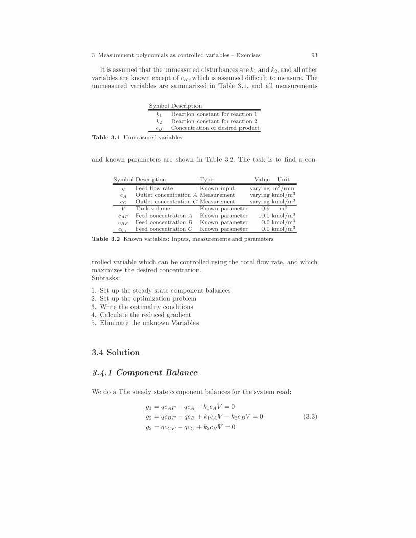
3 Measurement polynomials as controlled variables – Exercises 93
It is assumed that the unmeasured disturbances are k1 and k2, and all othervariables are known except of cB, which is assumed difficult to measure. Theunmeasured variables are summarized in Table 3.1, and all measurements
Symbol Description
k1 Reaction constant for reaction 1k2 Reaction constant for reaction 2cB Concentration of desired product
Table 3.1 Unmeasured variables
and known parameters are shown in Table 3.2. The task is to find a con-
Symbol Description Type Value Unit
q Feed flow rate Known input varying m3/mincA Outlet concentration A Measurement varying kmol/m3
cC Outlet concentration C Measurement varying kmol/m3
V Tank volume Known parameter 0.9 m3
cAF Feed concentration A Known parameter 10.0 kmol/m3
cBF Feed concentration B Known parameter 0.0 kmol/m3
cCF Feed concentration C Known parameter 0.0 kmol/m3
Table 3.2 Known variables: Inputs, measurements and parameters
trolled variable which can be controlled using the total flow rate, and whichmaximizes the desired concentration.Subtasks:
1. Set up the steady state component balances2. Set up the optimization problem3. Write the optimality conditions4. Calculate the reduced gradient5. Eliminate the unknown Variables
3.4 Solution
3.4.1 Component Balance
We do a The steady state component balances for the system read:
g1 = qcAF − qcA − k1cAV = 0
g2 = qcBF − qcB + k1cAV − k2cBV = 0
g2 = qcCF − qcC + k2cBV = 0
(3.3)
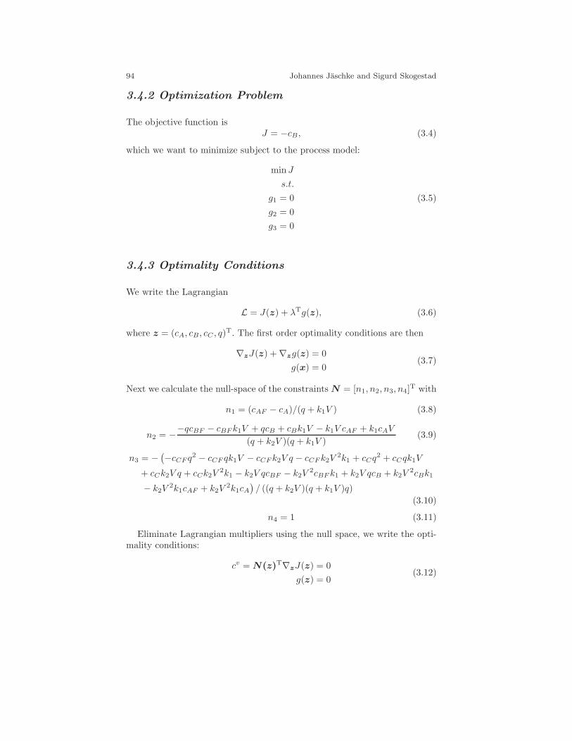
94 Johannes Jaschke and Sigurd Skogestad
3.4.2 Optimization Problem
The objective function isJ = −cB, (3.4)
which we want to minimize subject to the process model:
min J
s.t.
g1 = 0
g2 = 0
g3 = 0
(3.5)
3.4.3 Optimality Conditions
We write the Lagrangian
L = J(z) + λTg(z), (3.6)
where z = (cA, cB, cC , q)T. The first order optimality conditions are then
∇zJ(z) +∇zg(z) = 0
g(x) = 0(3.7)
Next we calculate the null-space of the constraints N = [n1, n2, n3, n4]T with
n1 = (cAF − cA)/(q + k1V ) (3.8)
n2 = −−qcBF − cBFk1V + qcB + cBk1V − k1V cAF + k1cAV
(q + k2V )(q + k1V )(3.9)
n3 = −(−cCF q
2 − cCF qk1V − cCFk2V q − cCFk2V2k1 + cCq
2 + cCqk1V
+ cCk2V q + cCk2V2k1 − k2V qcBF − k2V
2cBF k1 + k2V qcB + k2V2cBk1
− k2V2k1cAF + k2V
2k1cA)/ ((q + k2V )(q + k1V )q)
(3.10)
n4 = 1 (3.11)
Eliminate Lagrangian multipliers using the null space, we write the opti-mality conditions:
cv = N(z)T∇zJ(z) = 0
g(z) = 0(3.12)
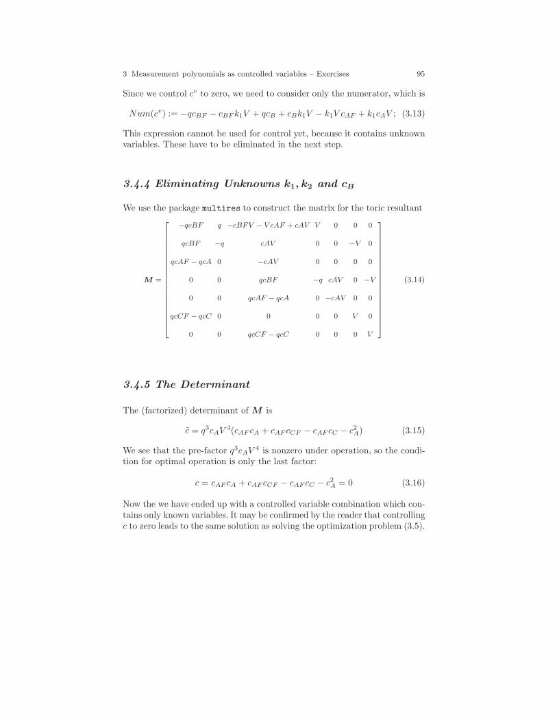
3 Measurement polynomials as controlled variables – Exercises 95
Since we control cv to zero, we need to consider only the numerator, which is
Num(cv) := −qcBF − cBFk1V + qcB + cBk1V − k1V cAF + k1cAV ; (3.13)
This expression cannot be used for control yet, because it contains unknownvariables. These have to be eliminated in the next step.
3.4.4 Eliminating Unknowns k1, k2 and cB
We use the package multires to construct the matrix for the toric resultant
M =
−qcBF q −cBFV − V cAF + cAV V 0 0 0
qcBF −q cAV 0 0 −V 0
qcAF − qcA 0 −cAV 0 0 0 0
0 0 qcBF −q cAV 0 −V
0 0 qcAF − qcA 0 −cAV 0 0
qcCF − qcC 0 0 0 0 V 0
0 0 qcCF − qcC 0 0 0 V
(3.14)
3.4.5 The Determinant
The (factorized) determinant of M is
c = q3cAV4(cAF cA + cAF cCF − cAF cC − c2A) (3.15)
We see that the pre-factor q3cAV4 is nonzero under operation, so the condi-
tion for optimal operation is only the last factor:
c = cAF cA + cAF cCF − cAF cC − c2A = 0 (3.16)
Now the we have ended up with a controlled variable combination which con-tains only known variables. It may be confirmed by the reader that controllingc to zero leads to the same solution as solving the optimization problem (3.5).

96 Johannes Jaschke and Sigurd Skogestad
3.4.6 Maple Code
The maple code for the CSTR example is given below
Maple code for the CSTR example
1 #################################################################
2 ## This is the file mapleCSTR.mpl
3 ## Simple CSTR
4 ## Johannes Jaeschke"
5 ## Nov. 2010
6 ################################################################
7
8 with(LinearAlgebra):with(VectorCalculus):
9 # Define the cost to minimize
10 J :=-cB;
11
12 # Setting up the constraints
13 g1 :=q*cAF - q*cA - k1*cA*V;
14 g2 :=q*cBF - q*cB + k1*cA*V - k2*cB*V;
15 g3 :=q*cCF - q*cC + k2*cB*V;
16 g :=[g1,g2,g3];
17
18 # Derive to obtain first order optimality constraints
19 Jac := Jacobian(g,[cA,cB,cC,q]);
20 gradT := Jacobian([J],[cA,cB,cC,q]);
21
22 # Calculate the null space of the constraints
23 N := NullSpace(Jac): N := N[1];
24
25 # Transpose and mutlitpy
26 G := Transpose(gradT):
27 NT := Transpose(N):
28 # The reduced gradient is then:
29 Cv := VectorMatrixMultiply(NT,G):
30 cv := simplify(numer(Cv[1])): # pick only numerator
31
32 # Unknown variables to be eliminated
33 read("multires.mpl"):
34 varlist := [k2,k1,cB]; #unknown variables
35 polylist:= [cv,g1,g2,g3]; #optimality conditions
36 BigMat := spresultant(polylist,varlist); #Construct resultant matrix
37 LargeMat:= det(BigMat); # Calculate determinant
38 c := factor(LargeMat); # factorize the CV
39 save Jac,grad,N,Cv,cv,c, "invariant"; # save results

3 Measurement polynomials as controlled variables – Exercises 97
Comments – Remarks

98 Johannes Jaschke and Sigurd Skogestad
Comments – Remarks

3 Measurement polynomials as controlled variables – Exercises 99
Comments – Remarks

100 Johannes Jaschke and Sigurd Skogestad
Comments – Remarks
Chapter 4
Multi-Parametric Toolbox
Michal Kvasnica
Abstract This chapter introduces the Multi-Parametric Toolbox (MPT) forMatlab, which is a freely-available tool for Model Predictive Control andcomputational geometry. MPT simplifies and automates many tasks a controlengineer has to go through when designing and validating optimal controllaws based on the MPC principle. The toolbox provides easy-to-use access tovarious tasks ranging from modeling of dynamical systems, through controlsynthesis, up to verification and code deployment. The purpose of this chapteris twofold. First, the toolbox is introduced and its functionality is explainedby means of simple, illuminating examples. Then, a set of advanced exercisesis provided for the reader to practice and master their skills.
4.1 Multi-Parametric Toolbox
Optimal control of constrained linear and piecewise affine systems has gar-nered great interest in the research community due to the ease with whichcomplex problems can be stated and solved. The aim of the Multi-ParametricToolbox (MPT) is to provide efficient computational means to obtain feed-back controllers for these types of constrained optimal control problems ina Matlab programming environment. As the name of the tool hints, it ismainly focused on calculation of feedback laws in the parametric fashion inwhich the feedback law takes a form of a PWA look-up table. But the toolboxis also able to formulate and solve MPC problems on-line in the receding hori-zon fashion, i.e. by solving the optimization problem for a particular value ofthe initial condition at each time step.
Michal KvasnicaFaculty of Chemical and Food Technology, Slovak University of Technologyin Bratislava, e-mail: [email protected]
101
102 Michal Kvasnica
In short, the Multi-Parametric Toolbox can be described as being a freeMatlab toolbox for design, analysis and deployment of MPC-based con-trol laws for constrained linear, nonlinear and hybrid systems. Efficiency ofthe code is guaranteed by the extensive library of algorithms from the fieldof computational geometry and multi-parametric optimization. The toolboxoffers a broad spectrum of algorithms compiled in a user friendly and ac-cessible format: starting from modeling systems which combine continuousdynamics with discrete logic (hybrid systems), through design of control lawsbased on different performance objectives (linear, quadratic, minimum time)to the handling of systems with persistent additive and polytopic uncertain-ties. Users can add custom constraints, such as polytopic, contraction, orcollision avoidance constraints, or create custom objective functions. Result-ing optimal control laws can either be embedded into control applicationsin the form of a C code, or deployed to target platforms using Real TimeWorkshop.
MPT can also be viewed as a unifying repository of hybrid systems de-sign tools from international experts utilizing state-of-the-art optimizationpackages. The list of included software packages includes packages for linearprogramming (CDD, GLPK), quadratic programming (CLP), mixed-integerlinear programming (GLPK), and semi-definite programming (SeDuMi). Inaddition, MPT ships with a dedicated solver for computing projections ofconvex polytopes, called ESP, a boolean optimization package ESPRESSO,as well as with the HYSDEL modeling language.
The main factor which distinguishes this toolbox from other alternativesis the big emphasis on efficient formulation of the problems which are beingsolved. This means that the toolbox provides implementation of novel controldesign and analysis algorithms, but also offers the user an easy way to usethem without the need to be an expert in the respective fields. MPT aimsat providing tools which can be used in the whole chain of the process ofsuccessful control design. It allows users not only to design optimization-based controllers, but also to formally verify that they behave as desired,investigate the behavior of the closed-loop system, and to post-process theresulting feedback laws in order to simplify them without loosing prescribeddesign properties.
4.1.1 Download and Installation
MPT is freely available for download from the project web site at http://control.ee.ethz.ch/˜mpt. After download, follow the installation instructionsand add all MPT’s subdirectories to Matlab path. To start off, check yourMPT installation by running the following command:
>> mpt_init
4 Multi-Parametric Toolbox 103
which should provide the output similar to this one:
looking for available solvers...
MPT toolbox 2.6.3 initialized...
LP solver: CDD Criss-Cross
QP solver: quadprog
MILP solver: GLPKCC
MIQP solver: YALMIP
Vertex enumeration: CDD
Any questions, suggestions and/or bug reports should be communicated [email protected].
4.2 Computational Geometry in MPT
4.2.1 Polytopes
First we introduce the computational geometry features of MPT. MPT con-tains a rich library for manipulating convex geometrical objects known aspolytopes.
Definition 4.1 (Convex Set). A set C ⊆ Rn is convex if the line segmentconnecting any two points in C lies entirely in C, i.e. θx1 + (1− θ)x2 ⊆ C forall x1, x2 ∈ C and θ ∈ R, 0 ≤ θ ≤ 1.
Definition 4.2 (Polyhedron). Convex set represented as the intersectionof a finite number of closed half-spaces aTi x ≤ bi, i.e. P = x ∈ Rn | Ax ≤ bwith
A =
aT1...
aTm
, b =
b1...bm
(4.1)
is called a polyhedron.
Definition 4.3 (Polytope). Polytope is a bounded polyhedron.
In general, polytopes can be described in two possible representations:
1. The H-representation, i.e. P = x | Ax ≤ b, where the input data A andb are matrices representing the defining half-spaces aTi x ≤ bi, or
2. the V-representation, i.e. P = convhx1, . . . , xm, where convh denotesthe convex hull operator, i.e. convhx1, . . . , xm = x | x = λ1x1 + · · ·+λmxm, 0 ≤ λi ≤ 1,
∑λi = 1. Here, the input data are the vertices
x1, . . . , xm of the polytope.

104 Michal Kvasnica
In MPT, polytopes are constructed using the polytope constructor1:
% define a triangle using inequalities
% x1 + x2 <= 1
% -x1 + x2 <= 1
% -x2 <= 0
A = [1 1; -1 1; 0 -1];
b = [1; 1; 0];
TH = polytope(A, b)
% define the triangle using vertices
x1 = [1; 0]; x2 = [-1; 0]; x3 = [0; 1];
TV = polytope([x1 x2 x3]’) % notice the transpose!
Calling the constructor returns a polytope object which can be processed inmultiple ways. Let us start by simple plots:
% plot the first polytope in a new window using red color
figure; plot(TH, ’r’);
% plot the first polytope in a new window using green color
figure; plot(TV, ’g’)
−1 −0.8 −0.6 −0.4 −0.2 0 0.2 0.4 0.6 0.8 10
0.1
0.2
0.3
0.4
0.5
0.6
0.7
0.8
0.9
1
x1
x 2
(a)
−1 −0.8 −0.6 −0.4 −0.2 0 0.2 0.4 0.6 0.8 10
0.1
0.2
0.3
0.4
0.5
0.6
0.7
0.8
0.9
1
x1
x 2
(b)
Fig. 4.1 Plot of polytopes TH (left) and TV (right).
The output of these commands is shown in Figure 4.1. It appears that thetwo polytopes are equal. But how to check this in an automated fashion?Easily, use the standard equivalence == Matlab operator:
% are they really equal?
TH == TV
ans =
1 See help polytope for more information.
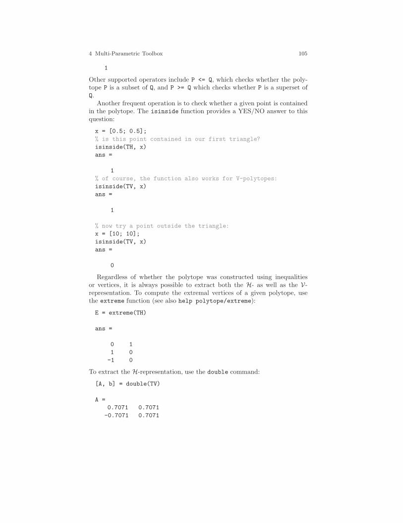
4 Multi-Parametric Toolbox 105
1
Other supported operators include P <= Q, which checks whether the poly-tope P is a subset of Q, and P >= Q which checks whether P is a superset ofQ.
Another frequent operation is to check whether a given point is containedin the polytope. The isinside function provides a YES/NO answer to thisquestion:
x = [0.5; 0.5];
% is this point contained in our first triangle?
isinside(TH, x)
ans =
1
% of course, the function also works for V-polytopes:
isinside(TV, x)
ans =
1
% now try a point outside the triangle:
x = [10; 10];
isinside(TV, x)
ans =
0
Regardless of whether the polytope was constructed using inequalitiesor vertices, it is always possible to extract both the H- as well as the V-representation. To compute the extremal vertices of a given polytope, usethe extreme function (see also help polytope/extreme):
E = extreme(TH)
ans =
0 1
1 0
-1 0
To extract the H-representation, use the double command:
[A, b] = double(TV)
A =
0.7071 0.7071
-0.7071 0.7071

106 Michal Kvasnica
0 -1.0000
b =
0.7071
0.7071
0
Notice that in this output all rows of A,b have been automatically normalizedsuch that the 2-norm of each row is equal to one to improve numerics.
4.2.2 Polytope Arrays
Instances of the polytope object can be concatenated into arrays. Currently,only one-dimensional arrays are supported by MPT and it does not matterif the elements are stored row-wise or column-wise. An array of polytopesis created using standard Matlab concatenation operators [,], e.g. A =
[B, C, D].It does not matter whether the concatenated elements are single poly-
topes or polyarrays. To illustrate this, assume that we have defined polytopesP1, P2, P3, P4, P5 and polyarrays A = [P1 P2] and B = [P3 P4 P5].Then the following polyarrays M and N are equivalent:
M = [A B]
N = [P1 P2 P3 P4 P5]
Individual elements of a polyarray can be obtained using the standard refer-encing (i) operator, i.e.
P = M(2)
will return the second element of the polyarray M which is equal to P2 in thiscase. More complicated expressions can be used for referencing:
Q = M([1,3:5])
will return a polyarray Q which contains first, third, fourth and fifth elementof polyarray M.
If the user wants to remove some element from a polyarray, he/she canuse the referencing command as follows:
M(2) = []
which will remove the second element from the polyarray M. Again, multipleindices can be specified, e.g.
M([1 3]) = []
will erase first and third element of the given polyarray. If some element of apolyarray is deleted, the remaining elements are shifted towards the start ofthe polyarray. This means that, assuming N = [P1 P2 P3 P4 P5], after
4 Multi-Parametric Toolbox 107
N([1 3]) = []
the polyarray N = [P2 P4 P5] and the length of the array is 3. No emptypositions in a polyarray are allowed. Similarly, empty polytopes are not beingadded to a polyarray.
A polyarray is still a polytope object, hence all functions which work onpolytopes support also polyarrays. This is an important feature mainly in thegeometric functions. Length of a given polyarray is obtained by
l = length(N)
A polyarray can be flipped by the following command:
Nf = fliplr(N)
i.e. if N = [P1 P2 P3 P4 P5] then Nf = [P5 P4 P3 P2 P1].
4.2.3 Operations on Polytopes
Next, we review some standard operations on polytopes.
4.2.3.1 Chebyshev Ball
The Chebychev’s ball of a polytope P = x ∈ Rn | Ax ≤ b is the largesthyperball inscribed in P , i.e. Br(xc) = x ∈ R
n | ‖x − xc‖2 ≤ r, such thatBr ⊆ P . The center and radius of such a hyperball can be easily found bysolving the following LP:
max r (4.2a)
subj. to Aixc + r‖Ai‖2 ≤ bi, (4.2b)
where Ai denotes the i-th row of A. The polytope P is empty if and only ifthe LP (4.2) is infeasible. If r = 0, then the polytope is lower dimensional.Note that the center of the Chebychev Ball is not unique, in general, i.e. therecan be multiple solutions (e.g. for rectangles).
Given a polytope object P, the center and radius of its Chebyshev’s ballcan be computed by calling the chebyball function:
>> [xc, r] = chebyball(P)
A sample Chebyshev’s ball inscribed in a 2D polytope is shown in Figure 4.2.
4.2.3.2 Affine Transformations
Consider a polytope P = x ∈ Rn | Ax ≤ b and an affine function f(x) =Fx + g with F ∈ Rn×n and g ∈ Rn, F non-singular. Then the image of the
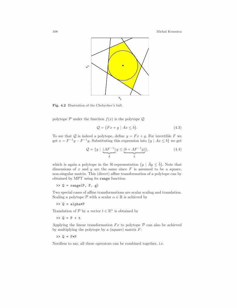
108 Michal Kvasnica
x1
x 2
Fig. 4.2 Illustration of the Chebychev’s ball.
polytope P under the function f(x) is the polytope Q
Q = Fx+ g | Ax ≤ b. (4.3)
To see that Q is indeed a polytope, define y = Fx + g. For invertible F weget x = F−1y − F−1g. Substituting this expression into y | Ax ≤ b we get
Q = y | (AF−1)︸ ︷︷ ︸A
y ≤ (b+AF−1g)︸ ︷︷ ︸b
, (4.4)
which is again a polytope in the H-representation y | Ay ≤ b. Note thatdimensions of x and y are the same since F is assumed to be a square,non-singular matrix. This (direct) affine transformation of a polytope can byobtained by MPT using its range function:
>> Q = range(P, F, g)
Two special cases of affine transformations are scalar scaling and translation.Scaling a polytope P with a scalar α ∈ R is achieved by
>> Q = alpha*P
Translation of P by a vector t ∈ Rn is obtained by
>> Q = P + t
Applying the linear transformation Fx to polytope P can also be achievedby multiplying the polytope by a (square) matrix F :
>> Q = F*P
Needless to say, all these operators can be combined together, i.e.
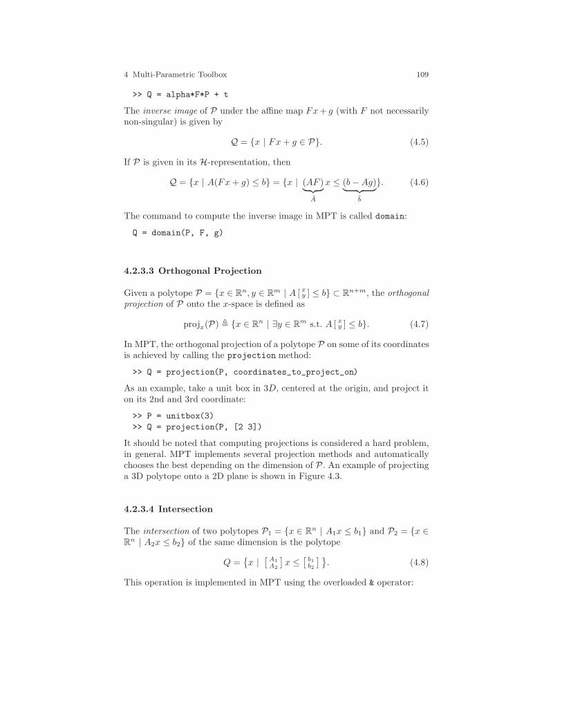
4 Multi-Parametric Toolbox 109
>> Q = alpha*F*P + t
The inverse image of P under the affine map Fx+ g (with F not necessarilynon-singular) is given by
Q = x | Fx+ g ∈ P. (4.5)
If P is given in its H-representation, then
Q = x | A(Fx+ g) ≤ b = x | (AF )︸ ︷︷ ︸A
x ≤ (b−Ag)︸ ︷︷ ︸b
. (4.6)
The command to compute the inverse image in MPT is called domain:
Q = domain(P, F, g)
4.2.3.3 Orthogonal Projection
Given a polytope P = x ∈ Rn, y ∈ Rm | A [ xy ] ≤ b ⊂ Rn+m, the orthogonalprojection of P onto the x-space is defined as
projx(P) , x ∈ Rn | ∃y ∈ R
m s.t. A [ xy ] ≤ b. (4.7)
In MPT, the orthogonal projection of a polytope P on some of its coordinatesis achieved by calling the projection method:
>> Q = projection(P, coordinates_to_project_on)
As an example, take a unit box in 3D, centered at the origin, and project iton its 2nd and 3rd coordinate:
>> P = unitbox(3)
>> Q = projection(P, [2 3])
It should be noted that computing projections is considered a hard problem,in general. MPT implements several projection methods and automaticallychooses the best depending on the dimension of P . An example of projectinga 3D polytope onto a 2D plane is shown in Figure 4.3.
4.2.3.4 Intersection
The intersection of two polytopes P1 = x ∈ Rn | A1x ≤ b1 and P2 = x ∈Rn | A2x ≤ b2 of the same dimension is the polytope
Q =x |
[A1
A2
]x ≤
[b1b2
] . (4.8)
This operation is implemented in MPT using the overloaded & operator:

110 Michal Kvasnica
Fig. 4.3 Illustration of orthogonal projection.
>> Q = P1 & P2
Note that MPT only computes full-dimensional intersections. Full dimen-sionality of the result Q can be checked by isfulldim(Q). An example of theintersection operation is shown in Figure 4.4.
−1 −0.8 −0.6 −0.4 −0.2 0 0.2 0.4 0.6 0.8 1−0.4
−0.2
0
0.2
0.4
0.6
0.8
1
x1
x 2
Fig. 4.4 Full-dimensional intersection of two polytopes.
4.2.3.5 Convex Hull
The convex hull of two or more polytopes Pi, i = 1, . . . ,m is the smallestconvex set which contains them, i.e.:
Q = convhvert(P1), . . . , vert(Pm), (4.9)
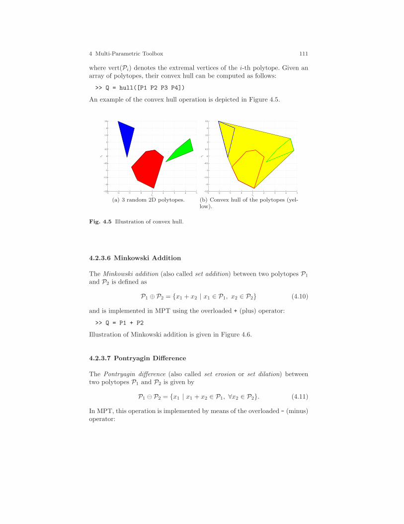
4 Multi-Parametric Toolbox 111
where vert(Pi) denotes the extremal vertices of the i-th polytope. Given anarray of polytopes, their convex hull can be computed as follows:
>> Q = hull([P1 P2 P3 P4])
An example of the convex hull operation is depicted in Figure 4.5.
−3 −2 −1 0 1 2 3 4 5−2.5
−2
−1.5
−1
−0.5
0
0.5
1
1.5
2
2.5
x1
x 2
(a) 3 random 2D polytopes.
−3 −2 −1 0 1 2 3 4 5−2.5
−2
−1.5
−1
−0.5
0
0.5
1
1.5
2
2.5
x1
x 2(b) Convex hull of the polytopes (yel-low).
Fig. 4.5 Illustration of convex hull.
4.2.3.6 Minkowski Addition
The Minkowski addition (also called set addition) between two polytopes P1
and P2 is defined as
P1 ⊕ P2 = x1 + x2 | x1 ∈ P1, x2 ∈ P2 (4.10)
and is implemented in MPT using the overloaded + (plus) operator:
>> Q = P1 + P2
Illustration of Minkowski addition is given in Figure 4.6.
4.2.3.7 Pontryagin Difference
The Pontryagin difference (also called set erosion or set dilation) betweentwo polytopes P1 and P2 is given by
P1 ⊖ P2 = x1 | x1 + x2 ∈ P1, ∀x2 ∈ P2. (4.11)
In MPT, this operation is implemented by means of the overloaded - (minus)operator:
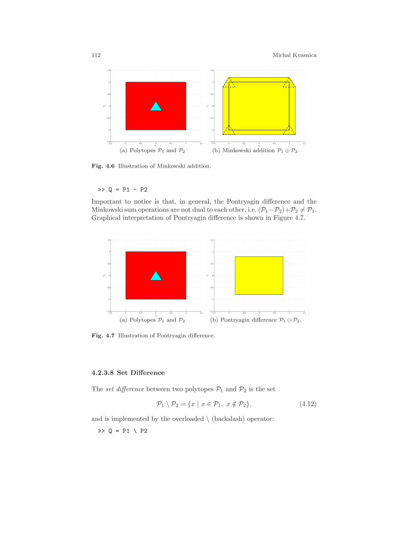
112 Michal Kvasnica
−1.5 −1 −0.5 0 0.5 1 1.5−1.5
−1
−0.5
0
0.5
1
1.5
x1
x 2
(a) Polytopes P1 and P2
−1.5 −1 −0.5 0 0.5 1 1.5−1.5
−1
−0.5
0
0.5
1
1.5
x1
x 2
(b) Minkowski addition P1 ⊕ P2.
Fig. 4.6 Illustration of Minkowski addition.
>> Q = P1 - P2
Important to notice is that, in general, the Pontryagin difference and theMinkowski sum operations are not dual to each other, i.e. (P1−P2)+P2 6= P1.Graphical interpretation of Pontryagin difference is shown in Figure 4.7.
−1.5 −1 −0.5 0 0.5 1 1.5−1.5
−1
−0.5
0
0.5
1
1.5
x1
x 2
(a) Polytopes P1 and P2
−1.5 −1 −0.5 0 0.5 1 1.5−1.5
−1
−0.5
0
0.5
1
1.5
x1
x 2
(b) Pontryagin difference P1 ⊖P2.
Fig. 4.7 Illustration of Pontryagin difference.
4.2.3.8 Set Difference
The set difference between two polytopes P1 and P2 is the set
P1 \ P2 = x | x ∈ P1, x /∈ P2, (4.12)
and is implemented by the overloaded \ (backslash) operator:
>> Q = P1 \ P2
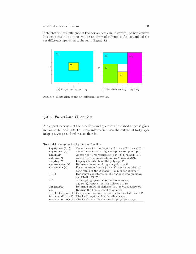
4 Multi-Parametric Toolbox 113
Note that the set difference of two convex sets can, in general, be non-convex.In such a case the output will be an array of polytopes. An example of theset difference operation is shown in Figure 4.8.
x1
x 2 P1
P2
(a) Polytopes P1 and P2
x1
x 2
Q1
Q2
Q3
Q4
(b) Set difference Q = P1 \ P2.
Fig. 4.8 Illustration of the set difference operation.
4.2.4 Functions Overview
A compact overview of the functions and operators described above is givenin Tables 4.1 and 4.2. For more information, see the output of help mpt,help polytope and references therein.
Table 4.1 Computational geometry functions
P=polytope(A,b) Constructor for the polytope P = x ∈ Rn | Ax ≤ b.P=polytope(V) Constructor for creating a V-represented polytopedouble(P) Access the H-representation, e.g. [A,b]=double(P).extreme(P) Access the V-representation, e.g. V=extreme(P).display(P) Displays details about the polytope P.nx=dimension(P) Returns dimension of a given polytope Pnc=nconstr(P) For a polytope P = x | Ax ≤ b returns number of
constraints of the A matrix (i.e. number of rows).[ , ] Horizontal concatenation of polytopes into an array,
e.g. PA=[P1,P2,P3].( ) Subscripting operator for polytope arrays,
e.g. PA(i) returns the i-th polytope in PA.length(PA) Returns number of elements in a polytope array PA.end Returns the final element of an array.[c,r]=chebyball(P) Center c and radius r of the Chebychev ball inside P.bool=isfulldim(P) Checks if polytope P is full dimensional.bool=isinside(P,x) Checks if x ∈ P. Works also for polytope arrays.

114 Michal Kvasnica
Table 4.2 Operators defined for polytope objects
P == Q Check if two polytopes are equal (P = Q).P ∼= Q Check if two polytopes are not-equal (P 6= Q).P >= Q Check if P ⊇ Q.P <= Q Check if P ⊆ Q.P > Q Check if P ⊃ Q.P < Q Check if P ⊂ Q.P & Q Intersection of two polytopes, P ∩ Q.P | Q Union of two polytopes, P ∪ Q.P + Q Minkowski sum, P ⊕Q (cf. (4.10)).P - Q Pontryagin difference, P ⊖Q (cf. (4.11)).P \ Q Set difference operator (cf. (4.12)).B=bounding_box(P) Minimal hyper-rectangle containing a polytope P.Q=range(P,A,f) Affine transformation of a polytope.
Q = Ax+ f | x ∈ P.Q=domain(P,A,f) Compute polytope that is mapped to P.
Q = x | Ax+ f ∈ P.R=projection(P,dim) Orthogonal projection of P onto coordinates
given in dim (cf. (4.7))

4 Multi-Parametric Toolbox 115
4.3 Exercises
Exercise 4.1. Perform following tasks:
1. Create a polytope P as the 2D unit box centered at the origin, i.e. P =(x1, x2)
T | − 1 ≤ x1 ≤ 1, − 1 ≤ x2 ≤ 1.2. Create an another polytope Q as the convex hull of points v1 = (−1, 0)T ,
v2 = (1, 0)T , v3 = (0, 1)T .3. Plot P in red and Q in blue (don’t forget to use figure to open a new
plot).4. Is P a subset of Q? Check this using vertices of Q.5. Is Q as subset of P? Check this using vertices of P.
Exercise 4.2. MPT offers an easy way to perform affine transformations ofpolytopes. These include:
• Shifting the polytope P in the direction given by a vector v leads a newpolytope R = x+ v | x ∈ P. It can by obtained by:v = [0.8; 1.4]; R = P + v
• Scaling P by a scalar factor α 6= 0 gives R = αx | x ∈ P:alpha = 0.6; R = alpha*P
• Affine transformation of P by an invertible matrix M gives R = Mx | x ∈P:M = [1.5 0; 0 1]; R = M*P
Now practice on the triangle defined in Exercise 1:
1. Let Q1 denote the shift of Q in the direction of the vector (0.5, − 0.2)T
2. Let Q2 be Q1 scaled by a factor of 0.83. Let Q3 represent Q2 rotated by 45o
4. Plot Q in red, Q1 in green, Q2 in blue and Q3 in magenta. Moreover, plotall polytopes in the same graph using wireframe.
Hints:
• Rotation is achieved by applying the following matrix transformation withθ being the angle in radians:
M =
[cos(θ) −sin(θ)sin(θ) cos(θ)
](4.13)
• To plot several polytopes in the same graph, do it in a standard Matlab
fashion, i.e. plot(P1, ’r’, P2, ’b’, ’P3’, ’g’)
• To plot using wireframe, use additional options:
opts = struct(’wire’, 1, ’linewidth’, 3);
plot(P1, ’r’, P2, ’b’, P3, ’g’, opts)

116 Michal Kvasnica
Exercise 4.3. Now concentrate only on Q and Q3 from the previous exercise.It is obvious from the plot that these two polytopes overlap, i.e. they have anon-empty intersection. To check this, use dointersect:
dointersect(Q3, Q)
ans =
1
Since the intersection of any two polytopes is again a polytope, the intersec-tion can be computed explicitly by calling the overloaded & operator:
Q4 = Q3 & Q
To visualize the intersection, we plot Q4 in solid yellow and Q3 and Q usingwireframes:
% a combined solid and wireframe plot cannot be achieved
% by a single command, therefore we split it in two steps:
opts = struct(’wire’, 1, ’linewidth’, 3);
plot(Q4, ’y’);
hold on; plot(Q, ’r’, Q3, ’m’, opts); hold off
−1 −0.8 −0.6 −0.4 −0.2 0 0.2 0.4 0.6 0.8 1−0.4
−0.2
0
0.2
0.4
0.6
0.8
1
x1
x 2
Fig. 4.9 Intersection of polytopes Q3 and Q.
Now practice: Plot the intersection of Q, Q2 and Q3.Hint: you can use & in a chain, i.e. Q & Q2 & Q3.
Exercise 4.4. The set difference operation between polytopes P and Q isdefined asP \Q = x | x ∈ P, x /∈ Q. In MPT, this is achieved by using the \ operator:
D = Q3 \ Q;
plot(D, ’g’)
hold on; plot(Q, ’r’, Q3, ’m’, opts); hold off

4 Multi-Parametric Toolbox 117
Notice that the set difference between two convex sets is not necessarily con-vex. In fact, the example above illustrates such case and we have D representedas an array of two polytopes:
D
D=
Polytope array: 2 polytopes in 2D
The number of elements of D can be determined by length(D) and its com-ponents can be accessed using standard Matlab indexing, e.g.
D1 = D(1);
D2 = D(2);
D3 = D(end); % same as D(2)
You can also create a polytope array on your own, e.g.
polyarray = [D(1) Q D(2) Q3]
Now practice: Plot the set difference between Q and Q3 (notice that orderingmakes a difference). How many polytopes define the difference?
Exercise 4.5. The Minkowski addition operation P1 ⊕P2, described in Sec-tion 4.2.3.6, is easy to implement of the polytopes P1 and P2 are given intheir V-representation, i.e. P1 = convhx1, . . . , xm, P2 = convhy1, . . . , yp.Then
P1 ⊕ P2 = convhxi + yj , ∀i, ∀j. (4.14)
Now assume that P1 and P2 are as follows:
>> P1 = unitbox(2)
>> P2 = unitbox(2)*0.1
−1 −0.8 −0.6 −0.4 −0.2 0 0.2 0.4 0.6 0.8 1−0.4
−0.2
0
0.2
0.4
0.6
0.8
1
x1
x 2
Fig. 4.10 Set difference between Q3 and Q.
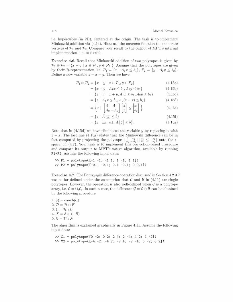
118 Michal Kvasnica
i.e. hypercubes (in 2D), centered at the origin. The task is to implementMinkowski addition via (4.14). Hint: use the extreme function to enumeratevertices of P1 and P2. Compare your result to the output of MPT’s internalimplementation, i.e. to P1+P2.
Exercise 4.6. Recall that Minkowski addition of two polytopes is given byP1 ⊕ P2 = x + y | x ∈ P1, y ∈ P2 . Assume that the polytopes are givenby their H-representation, i.e. P1 = x | A1x ≤ b1, P2 = y | A2y ≤ b2.Define a new variable z = x+ y. Then we have
P1 ⊕ P2 = x+ y | x ∈ P1, y ∈ P2 (4.15a)
= x+ y | A1x ≤ b1, A2y ≤ b2 (4.15b)
= z | z = x+ y,A1x ≤ b1, A2y ≤ b2 (4.15c)
= z | A1x ≤ b1, A2(z − x) ≤ b2 (4.15d)
=z |
[ 0 A1
A2 −A2
] [zx
]≤
[b1b2
](4.15e)
= z | A [ zx ] ≤ b (4.15f)
= z | ∃x, s.t. A [ zx ] ≤ b. (4.15g)
Note that in (4.15d) we have eliminated the variable y by replacing it withz − x. The last line (4.15g) states that the Minkowski difference can be infact computed by projecting the polytope
[0 A1
A2 −A2
][ zx ] ≤
[b1b2
]onto the z-
space, cf. (4.7). Your task is to implement this projection-based procedureand compare its output to MPT’s native algorithm, available by runningP1+P2. Assume the following input data:
>> P1 = polytope([-1 -1; -1 1; 1 -1; 1 1])
>> P2 = polytope([-0.1 -0.1; 0.1 -0.1; 0 0.1])
Exercise 4.7. The Pontryagin difference operation discussed in Section 4.2.3.7was so far defined under the assumption that C and B in (4.11) are singlepolytopes. However, the operation is also well-defined when C is a polytopearray, i.e. C = ∪iCi. In such a case, the difference G = C ⊖ B can be obtainedby the following procedure:
1. H = convh(C)2. D = H⊖ B3. E = H \ C4. F = E ⊕ (−B)5. G = D \ FThe algorithm is explained graphically in Figure 4.11. Assume the followinginput data:
>> C1 = polytope([0 -2; 0 2; 2 4; 2 -4; 4 2; 4 -2])
>> C2 = polytope([-4 -2; -4 2; -2 4; -2 -4; 0 -2; 0 2])
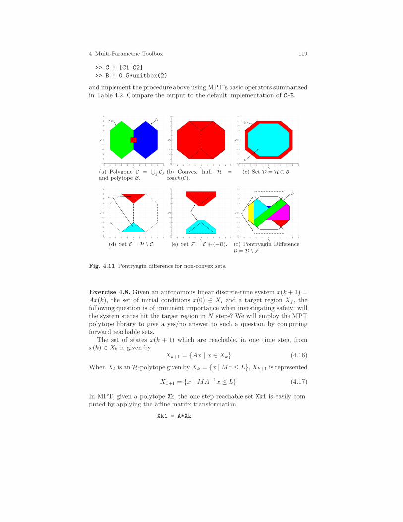
4 Multi-Parametric Toolbox 119
>> C = [C1 C2]
>> B = 0.5*unitbox(2)
and implement the procedure above using MPT’s basic operators summarizedin Table 4.2. Compare the output to the default implementation of C-B.
−5 −4 −3 −2 −1 0 1 2 3 4 5−5
−4
−3
−2
−1
0
1
2
3
4
5
x1
x 2
C2 C1
P1
(a) Polygone C =⋃
jCj
and polytope B.
−5 −4 −3 −2 −1 0 1 2 3 4 5−5
−4
−3
−2
−1
0
1
2
3
4
5
x1
x 2
(b) Convex hull H =convh(C).
−5 −4 −3 −2 −1 0 1 2 3 4 5−5
−4
−3
−2
−1
0
1
2
3
4
5
x1
x 2
H
D
(c) Set D = H⊖ B.
−5 −4 −3 −2 −1 0 1 2 3 4 5−5
−4
−3
−2
−1
0
1
2
3
4
5
x1
x 2
E
(d) Set E = H \ C.
−5 −4 −3 −2 −1 0 1 2 3 4 5−5
−4
−3
−2
−1
0
1
2
3
4
5
x1
x 2 F
(e) Set F = E ⊕ (−B).
−5 −4 −3 −2 −1 0 1 2 3 4 5−5
−4
−3
−2
−1
0
1
2
3
4
5
x1
x 2
D
F
(f) Pontryagin DifferenceG = D \ F .
Fig. 4.11 Pontryagin difference for non-convex sets.
Exercise 4.8. Given an autonomous linear discrete-time system x(k + 1) =Ax(k), the set of initial conditions x(0) ∈ Xi and a target region Xf , thefollowing question is of imminent importance when investigating safety: willthe system states hit the target region in N steps? We will employ the MPTpolytope library to give a yes/no answer to such a question by computingforward reachable sets.
The set of states x(k + 1) which are reachable, in one time step, fromx(k) ∈ Xk is given by
Xk+1 = Ax | x ∈ Xk (4.16)
When Xk is anH-polytope given byXk = x |Mx ≤ L,Xk+1 is represented
Xx+1 = x | MA−1x ≤ L (4.17)
In MPT, given a polytope Xk, the one-step reachable set Xk1 is easily com-puted by applying the affine matrix transformation
Xk1 = A*Xk
120 Michal Kvasnica
Assume the following input data:
A = [0.5, -0.75; 0.75, 0.5];
Xi = unitbox(2) + [3; 0]; % unit box centered at [3; 0]
Xf = 0.5*unitbox(2); % box with sides of +/- 0.5
% centered at [0; 0]
N = 10
Now answer the following questions:
1. Will the system states, starting from Xi, hit the target region in N steps?2. If no, by how much would N need to be increased?3. Plot the initial set, the terminal region and the reachable sets.
Hints:
• Apply (4.17) in a loop for k = 1:N starting with X1 = Xi.• Use a growing array to store the intermediate results, e.g.
R = polytope;
for k = 1:N
% compute polytope P
R = [R P]; % add P at the end of the array
end
• Use the dointersect function to detect hit of the target (remember Ex-ercise 5).
• You can plot the whole polytope array R in one shot by plot(R).
Exercise 4.9. Given is a discrete-time, LTI system xk+1 = Axk +Buk sub-ject to constraints xmin ≤ xk ≤ xmax, umin ≤ uk ≤ umax. Take the followingdata:
A =
[1 10 1
], B =
[10.5
], xmin =
[−5−5
], xmax =
[55
], umin = −1, umax = 1
Let’s stabilize the system by an LQR feedback uk = −Kxk with K = dlqr(A,
B, eye(2), 1), which gives K =[0.52 0.94
]. Obviously, such a controller
doesn’t take constraints into account.
However, there are some states for which all constraints are satisfied, e.g.
x = [0.1; 0.1]; % clearly satisfies state constraints
u = -K*x = -0.146; % clearly satisfies input constraints
and some for which they are violated, e.g.:
x = [1; 1]; % satisfies state constraints
u = -K*x = -1.46 % but violates input constraints
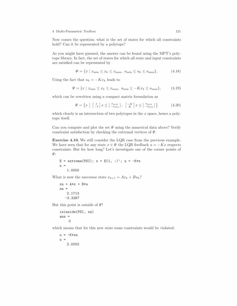
4 Multi-Parametric Toolbox 121
Now comes the question: what is the set of states for which all constraintshold? Can it be represented by a polytope?
As you might have guessed, the answer can be found using the MPT’s poly-tope library. In fact, the set of states for which all state and input constraintsare satisfied can be represented by
Ψ = x | xmin ≤ xk ≤ xmax, umin ≤ uk ≤ umax, (4.18)
Using the fact that uk = −Kxk leads to
Ψ = x | xmin ≤ xk ≤ xmax, umin ≤ −Kxk ≤ umax, (4.19)
which can be rewritten using a compact matrix formulation as
Ψ =x∣∣ [
I−I
]x ≤ [ xmax
−xmin] ,
[−KK
]x ≤ [ umax
−umin]
(4.20)
which clearly is an intersection of two polytopes in the x space, hence a poly-tope itself.
Can you compute and plot the set Ψ using the numerical data above? Verifyconstraint satisfaction by checking the extremal vertices of Ψ .
Exercise 4.10. We still consider the LQR case from the previous example.We have seen that for any state x ∈ Ψ the LQR feedback u = −Kx respectsconstraints. But for how long? Let’s investigate one of the corner points ofΨ :
E = extreme(PSI); x = E(1, :)’; u = -K*x
u =
1.0000
What is now the successor state xk+1 = Axk +Buk?
xn = A*x + B*u
xn =
2.1713
-3.3287
But this point is outside of Ψ !
isinside(PSI, xn)
ans =
0
which means that for this new state some constraints would be violated:
u = -K*xn
u =
2.0002
122 Michal Kvasnica
In other words, Ψ does not possess the set invariance property. In simplewords, a set Φ∞ is invariant if, for all starting points x0 inside such set, allfuture trajectories xk remain in the set ∀k ≥ 0. Set invariance is crucial forMPC in order to guarantee stability of the closed-loop system.
Now that we checked that Ψ is not invariant, can we compute its invariantsubset Φ∞? Following definition might help:
Φ∞ = xk | xk ∈ Ψ, (A−BK)xk ∈ Ψ, ∀k ≥ 0 (4.21)
Following iterative algorithm can be used to compute Φ∞:
Step 1: k = 1, Ψk = Ψ
Step 2: repeat
Step 3: Ψk+1 = x | x ∈ Ψk, (A−BK)x ∈ ΨkStep 4: k = k + 1
Step 5: until Ψk 6= Ψk−1
Step 6: Φ∞ = Ψk
The only non-trivial stage is Step 3. Remember the forward reach sets ofExample 4? Take a look again at (4.16) and you should spot some similarities.In fact, the set computed in Step 3 is the one-step backwards reachable set,i.e. the subset of Ψk which remains in Ψk for one time step. Since forwardreach sets were computed by Xk+1 = AXk, we can compute the backwardset by Xk+1 = A−1Xk, intersected with Xk itself, i.e.
PSI(k+1) = PSI(k) & inv(A-B*K)*PSI(k)
The rest of the solution should be clear. You will, however, need to replacerepeat-until by a while-end statement and negate the stopping conditionaccordingly.
Now it’s your turn: compute the invariant subset of PSI and plot it.
Note that many theoretical subtleties were untold in this story. One of thembeing that the presented algorithm has no guarantee of finite-time conver-gence, there you should place an upper limit on the number of iterations. 10is a safe choice.
4.4 Solutions
Solution 4.1 (for Exercise 4.1).
1. Create a polytope P as the 2D unit box centered at the origin, i.e. P =(x1, x2)
T | − 1 ≤ x1 ≤ 1, − 1 ≤ x2 ≤ 1.

4 Multi-Parametric Toolbox 123
% convert all inequalities into the form [a1 a2]*[x1; x2]
<= b:
% x_1 <= 1 i.e. [ 1 0]*[x1; x2] <= 1
% -x_1 <= 1 i.e. [-1 0]*[x1; x2] <= 1
% x_2 <= 1 i.e. [ 0 1]*[x1; x2] <= 1
% -x_2 <= 1 i.e. [ 0 -1]*[x1; x2] <= 1
% now stack all inequalities into a matrix:
A = [1 0; -1 0; 0 1; 0 -1];
b = [1; 1; 1; 1];
P = polytope(A, b);
2. Create an another polytope Q as the convex hull of points v1 = (−1, 0)T ,v2 = (1, 0)T , v3 = (0, 1)T .
v1 = [-0.5; 0]; v2 = [0.5; 0]; v3 = [0; 0.5];
Q = polytope([v1 v2 v3]’); % don’t forget the transpose!
3. Plot P in red and Q in blue (don’t forget to use figure to open a newplot).
figure; plot(P, ’r’)
figure; plot(Q, ’b’)
4. Is P a subset of Q? Check this using vertices of Q. Or a one-liner...
P <= Q
ans =
0
5. Is Q as subset of P? Check this using vertices of P. Or a one-liner...
Q <= P
ans =
1
Solution 4.2 (for Exercise 4.2).
1. Let Q1 denote the shift of Q in the direction of the vector (0.5, − 0.2)T
Q1 = Q + [0.5; -0.2];
2. Let Q2 be Q1 scaled by a factor of 0.8
Q2 = 0.8*Q1;
3. Let Q3 represent Q2 rotated by 45o
th = 45/180*pi; M = [cos(th) -sin(th); sin(th) cos(th)];
Q3 = M*Q2;
4. Plot Q in red, Q1 in green, Q2 in blue and Q3 in magenta. Moreover, plotall polytopes in the same graph using wireframe.
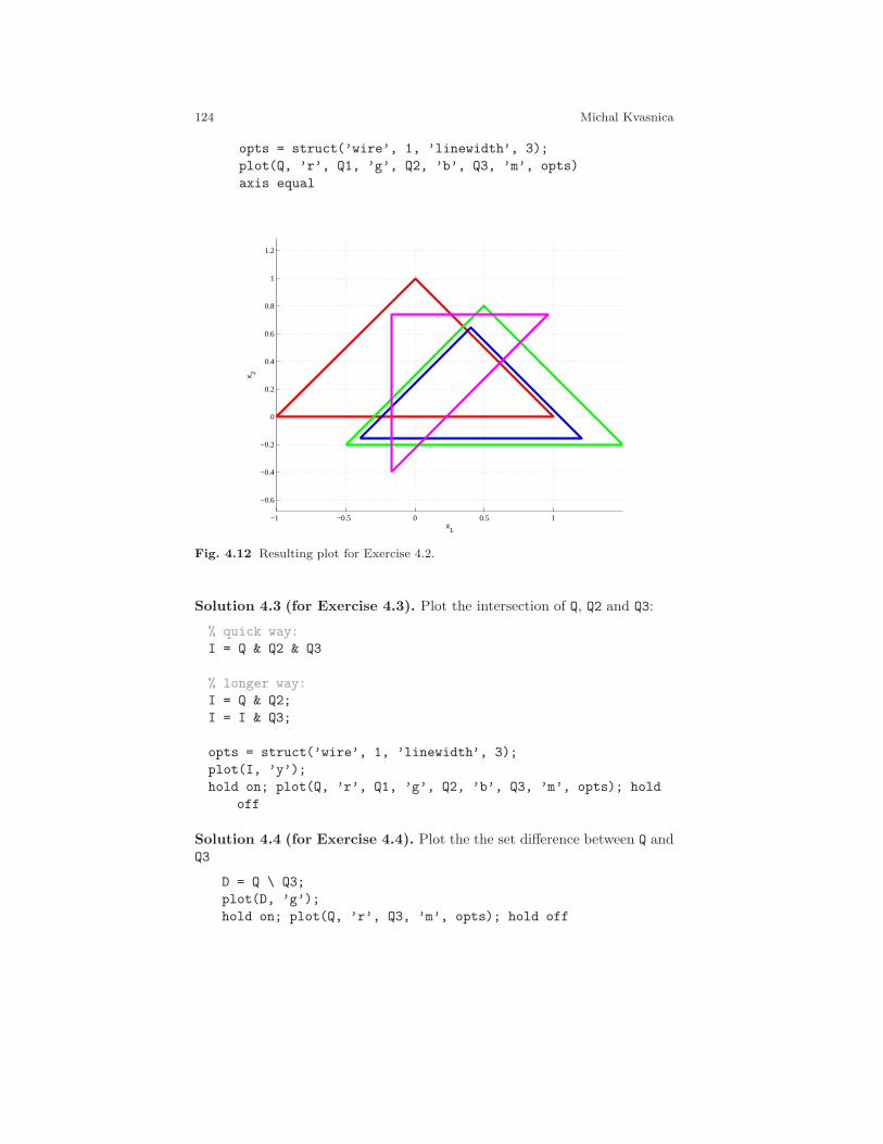
124 Michal Kvasnica
opts = struct(’wire’, 1, ’linewidth’, 3);
plot(Q, ’r’, Q1, ’g’, Q2, ’b’, Q3, ’m’, opts)
axis equal
−1 −0.5 0 0.5 1
−0.6
−0.4
−0.2
0
0.2
0.4
0.6
0.8
1
1.2
x1
x 2
Fig. 4.12 Resulting plot for Exercise 4.2.
Solution 4.3 (for Exercise 4.3). Plot the intersection of Q, Q2 and Q3:
% quick way:
I = Q & Q2 & Q3
% longer way:
I = Q & Q2;
I = I & Q3;
opts = struct(’wire’, 1, ’linewidth’, 3);
plot(I, ’y’);
hold on; plot(Q, ’r’, Q1, ’g’, Q2, ’b’, Q3, ’m’, opts); hold
off
Solution 4.4 (for Exercise 4.4). Plot the the set difference between Q andQ3
D = Q \ Q3;
plot(D, ’g’);
hold on; plot(Q, ’r’, Q3, ’m’, opts); hold off

4 Multi-Parametric Toolbox 125
−1 −0.5 0 0.5 1 1.5−0.4
−0.2
0
0.2
0.4
0.6
0.8
1
x1
x 2
Fig. 4.13 Intersection of polytopes Q, Q2, and Q3.
How many polytopes define the difference?
length(D)
ans =
3
Solution 4.5 (for Exercise 4.5).
% input data
P1 = unitbox(2);
P2 = unitbox(2)*0.1;
−1.5 −1 −0.5 0 0.5 1−0.5
0
0.5
1
x1
x 2
Fig. 4.14 Set difference between Q and Q3.
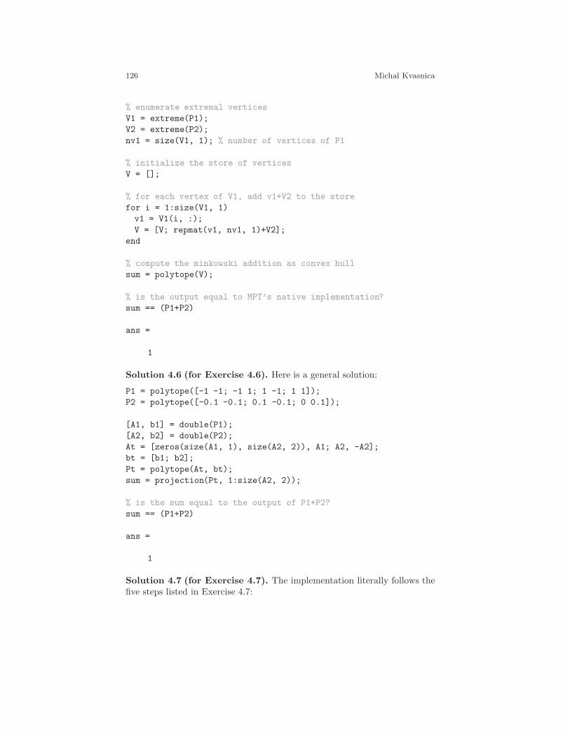
126 Michal Kvasnica
% enumerate extremal vertices
V1 = extreme(P1);
V2 = extreme(P2);
nv1 = size(V1, 1); % number of vertices of P1
% initialize the store of vertices
V = [];
% for each vertex of V1, add v1+V2 to the store
for i = 1:size(V1, 1)
v1 = V1(i, :);
V = [V; repmat(v1, nv1, 1)+V2];
end
% compute the minkowski addition as convex hull
sum = polytope(V);
% is the output equal to MPT’s native implementation?
sum == (P1+P2)
ans =
1
Solution 4.6 (for Exercise 4.6). Here is a general solution:
P1 = polytope([-1 -1; -1 1; 1 -1; 1 1]);
P2 = polytope([-0.1 -0.1; 0.1 -0.1; 0 0.1]);
[A1, b1] = double(P1);
[A2, b2] = double(P2);
At = [zeros(size(A1, 1), size(A2, 2)), A1; A2, -A2];
bt = [b1; b2];
Pt = polytope(At, bt);
sum = projection(Pt, 1:size(A2, 2));
% is the sum equal to the output of P1+P2?
sum == (P1+P2)
ans =
1
Solution 4.7 (for Exercise 4.7). The implementation literally follows thefive steps listed in Exercise 4.7:
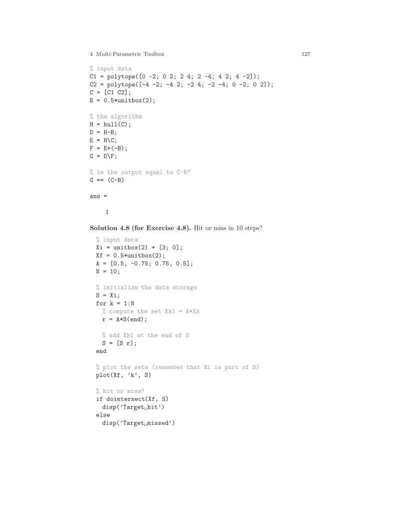
4 Multi-Parametric Toolbox 127
% input data
C1 = polytope([0 -2; 0 2; 2 4; 2 -4; 4 2; 4 -2]);
C2 = polytope([-4 -2; -4 2; -2 4; -2 -4; 0 -2; 0 2]);
C = [C1 C2];
B = 0.5*unitbox(2);
% the algorithm
H = hull(C);
D = H-B;
E = H\C;
F = E+(-B);
G = D\F;
% is the output equal to C-B?
G == (C-B)
ans =
1
Solution 4.8 (for Exercise 4.8). Hit or miss in 10 steps?
% input data
Xi = unitbox(2) + [3; 0];
Xf = 0.5*unitbox(2);
A = [0.5, -0.75; 0.75, 0.5];
N = 10;
% initialize the data storage
S = Xi;
for k = 1:N
% compute the set Xk1 = A*Xk
r = A*S(end);
% add Xk1 at the end of S
S = [S r];
end
% plot the sets (remember that Xi is part of S)
plot(Xf, ’k’, S)
% hit or miss?
if dointersect(Xf, S)
disp(’Target hit’)
else
disp(’Target missed’)
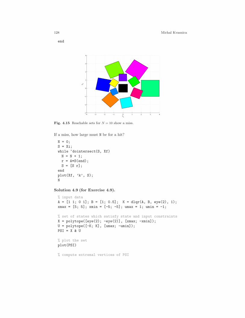
128 Michal Kvasnica
end
−4 −3 −2 −1 0 1 2 3 4−3
−2
−1
0
1
2
3
4
x1
x 2
Fig. 4.15 Reachable sets for N = 10 show a miss.
If a miss, how large must N be for a hit?
N = 0;
S = Xi;
while ~dointersect(S, Xf)
N = N + 1;
r = A*S(end);
S = [S r];
end
plot(Xf, ’k’, S);
N
Solution 4.9 (for Exercise 4.9).
% input data
A = [1 1; 0 1]; B = [1; 0.5]; K = dlqr(A, B, eye(2), 1);
xmax = [5; 5]; xmin = [-5; -5]; umax = 1; umin = -1;
% set of states which satisfy state and input constraints
X = polytope([eye(2); -eye(2)], [xmax; -xmin]);
U = polytope([-K; K], [umax; -umin]);
PSI = X & U
% plot the set
plot(PSI)
% compute extremal vertices of PSI
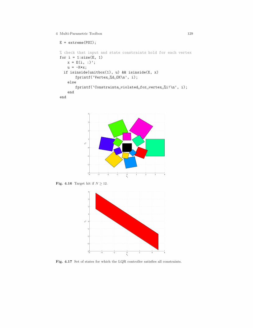
4 Multi-Parametric Toolbox 129
E = extreme(PSI);
% check that input and state constraints hold for each vertex
for i = 1:size(E, 1)
x = E(i, :)’;
u = -K*x;
if isinside(unitbox(1), u) && isinside(X, x)
fprintf(’Vertex %d OK\n’, i);
else
fprintf(’Constraints violated for vertex %i!\n’, i);
end
end
−4 −3 −2 −1 0 1 2 3 4−3
−2
−1
0
1
2
3
4
x1
x 2
Fig. 4.16 Target hit if N ≥ 12.
−6 −4 −2 0 2 4 6−4
−3
−2
−1
0
1
2
3
4
x1
x 2
Fig. 4.17 Set of states for which the LQR controller satisfies all constraints.
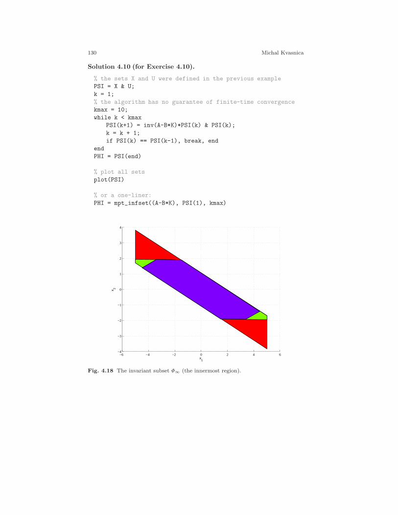
130 Michal Kvasnica
Solution 4.10 (for Exercise 4.10).
% the sets X and U were defined in the previous example
PSI = X & U;
k = 1;
% the algorithm has no guarantee of finite-time convergence
kmax = 10;
while k < kmax
PSI(k+1) = inv(A-B*K)*PSI(k) & PSI(k);
k = k + 1;
if PSI(k) == PSI(k-1), break, end
end
PHI = PSI(end)
% plot all sets
plot(PSI)
% or a one-liner:
PHI = mpt_infset((A-B*K), PSI(1), kmax)
−6 −4 −2 0 2 4 6−4
−3
−2
−1
0
1
2
3
4
x1
x 2
Fig. 4.18 The invariant subset Φ∞ (the innermost region).
4 Multi-Parametric Toolbox 131
4.5 Model Predictive Control in MPT
We consider the class of discrete-time, time-invariant systems given by thestate-space representation
x(t+ 1) = f(x(t), u(t)), (4.22)
where x(t) is the state vector at time t, x(t + 1) is the successor state, u(t)denotes the control input. Moreover, f(·, ·) is the state-update function whichdepends on the type of the model, which can either describe a linear time-invariant (LTI) system with
f(x(t), u(t)) = Ax(t) +Bu(t), (4.23)
or a Piecewise Affine (PWA) system with
f(x(t), u(t)) = Aix(t) +Biu(t) + fi if[x(t)u(t)
]∈ Di, (4.24)
where the state-update matrices change according to the position of the state-
input vector, i.e. the tuple (Ai, Bi, fi) is valid if[x(t)u(t)
]∈ Di, where Di, i =
1, . . . , D are polytopes of the state-input space. Furthermore, it is assumedthat the system variables are subject to constraints
x(t) ∈ X , u(t) ∈ U , ∀t ≥ 0, (4.25)
where X and U are polytopic sets.In MPC, optimal control actions are calculated by formulating and solving
a suitable optimization problem, which usually takes the following form:
minUN
‖PNxN‖p +N−1∑
k=0
‖Qxk‖p + ‖Ruk‖p (4.26a)
s.t. x0 = x(t), (4.26b)
xk+1 = f(xk, uk), k = 0, . . . , N − 1 (4.26c)
xk ∈ X , k = 0, . . . , N (4.26d)
uk ∈ U , k = 0, . . . , N − 1 (4.26e)
where xk and uk denote, respectively, the state and input predictions at timeinstants t+ k, initialized by the measurements of the current state x(t), andPN , Q, R are penalty matrices. The prediction is carried out over a finiteprediction horizon N . In addition, ‖Pz‖p with p = 2 stands for the square ofthe weighted 2-norm of z, i.e. zTPz. Similarly, p = 1 and p = ∞ denote the1- and ∞-norms of some vector.
The aim of MPC is to find the vector UN := [uT0 , u
T1 , . . . , u
TN−1]
T of optimalcontrol inputs which minimizes the cost function (4.26a). If f(·, ·) in (4.26c)
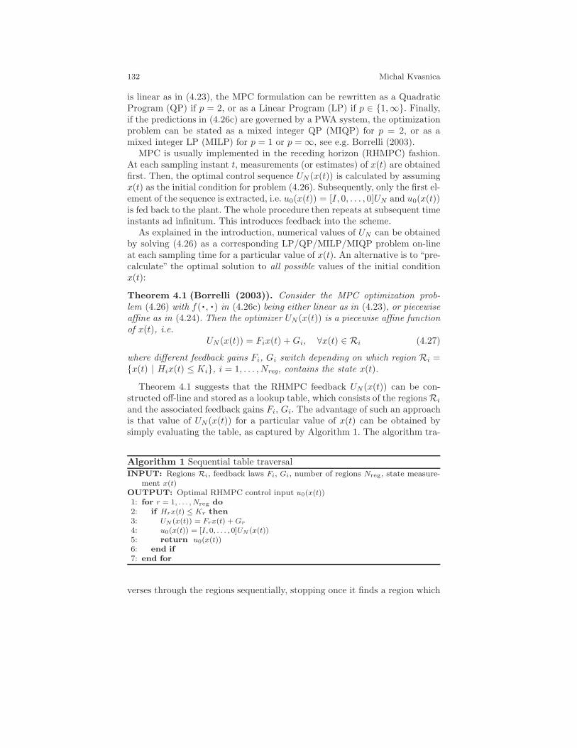
132 Michal Kvasnica
is linear as in (4.23), the MPC formulation can be rewritten as a QuadraticProgram (QP) if p = 2, or as a Linear Program (LP) if p ∈ 1,∞. Finally,if the predictions in (4.26c) are governed by a PWA system, the optimizationproblem can be stated as a mixed integer QP (MIQP) for p = 2, or as amixed integer LP (MILP) for p = 1 or p = ∞, see e.g. Borrelli (2003).
MPC is usually implemented in the receding horizon (RHMPC) fashion.At each sampling instant t, measurements (or estimates) of x(t) are obtainedfirst. Then, the optimal control sequence UN(x(t)) is calculated by assumingx(t) as the initial condition for problem (4.26). Subsequently, only the first el-ement of the sequence is extracted, i.e. u0(x(t)) = [I, 0, . . . , 0]UN and u0(x(t))is fed back to the plant. The whole procedure then repeats at subsequent timeinstants ad infinitum. This introduces feedback into the scheme.
As explained in the introduction, numerical values of UN can be obtainedby solving (4.26) as a corresponding LP/QP/MILP/MIQP problem on-lineat each sampling time for a particular value of x(t). An alternative is to “pre-calculate” the optimal solution to all possible values of the initial conditionx(t):
Theorem 4.1 (Borrelli (2003)). Consider the MPC optimization prob-lem (4.26) with f(·, ·) in (4.26c) being either linear as in (4.23), or piecewiseaffine as in (4.24). Then the optimizer UN(x(t)) is a piecewise affine functionof x(t), i.e.
UN (x(t)) = Fix(t) +Gi, ∀x(t) ∈ Ri (4.27)
where different feedback gains Fi, Gi switch depending on which region Ri =x(t) | Hix(t) ≤ Ki, i = 1, . . . , Nreg, contains the state x(t).
Theorem 4.1 suggests that the RHMPC feedback UN(x(t)) can be con-structed off-line and stored as a lookup table, which consists of the regionsRi
and the associated feedback gains Fi, Gi. The advantage of such an approachis that value of UN(x(t)) for a particular value of x(t) can be obtained bysimply evaluating the table, as captured by Algorithm 1. The algorithm tra-
Algorithm 1 Sequential table traversalINPUT: Regions Ri, feedback laws Fi, Gi, number of regions Nreg, state measure-
ment x(t)OUTPUT: Optimal RHMPC control input u0(x(t))1: for r = 1, . . . , Nreg do
2: if Hrx(t) ≤ Kr then
3: UN (x(t)) = Frx(t) +Gr
4: u0(x(t)) = [I, 0, . . . , 0]UN (x(t))5: return u0(x(t))6: end if
7: end for
verses through the regions sequentially, stopping once it finds a region which
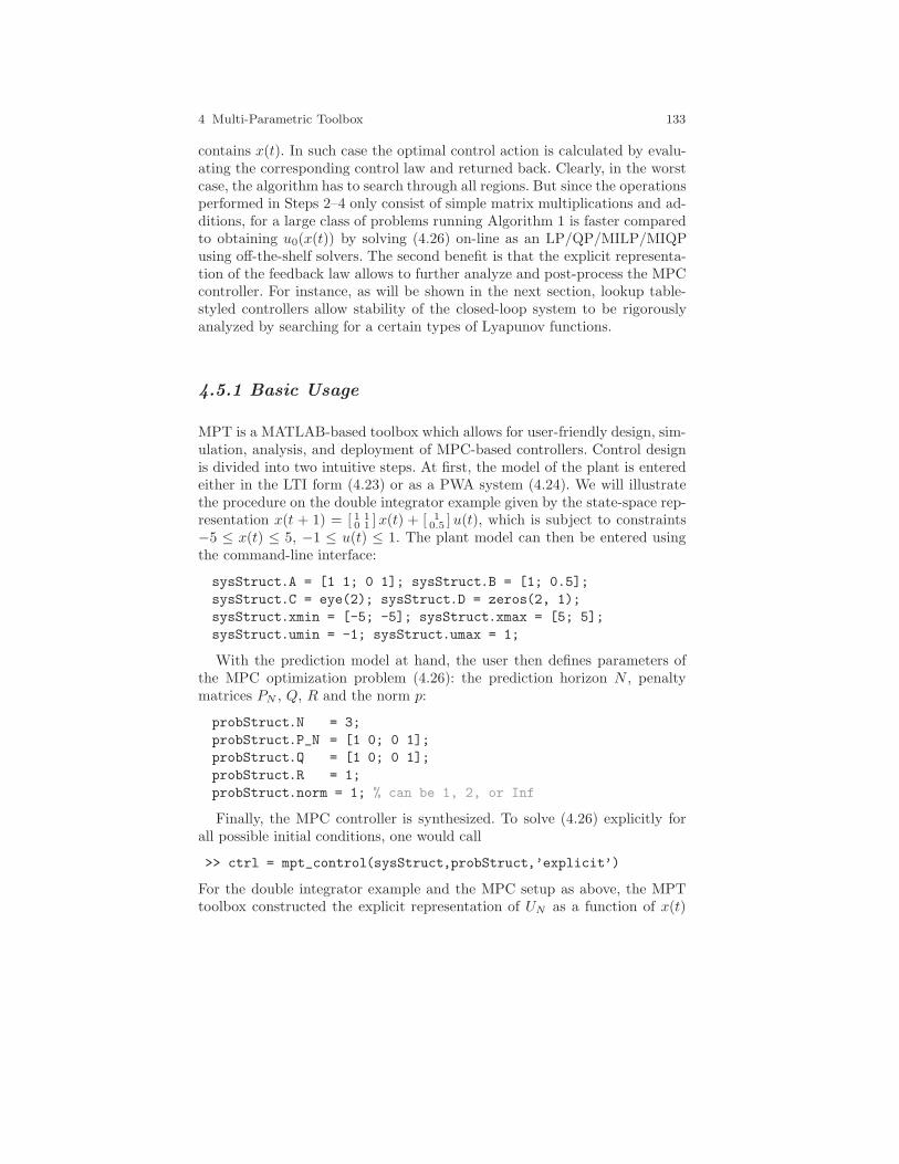
4 Multi-Parametric Toolbox 133
contains x(t). In such case the optimal control action is calculated by evalu-ating the corresponding control law and returned back. Clearly, in the worstcase, the algorithm has to search through all regions. But since the operationsperformed in Steps 2–4 only consist of simple matrix multiplications and ad-ditions, for a large class of problems running Algorithm 1 is faster comparedto obtaining u0(x(t)) by solving (4.26) on-line as an LP/QP/MILP/MIQPusing off-the-shelf solvers. The second benefit is that the explicit representa-tion of the feedback law allows to further analyze and post-process the MPCcontroller. For instance, as will be shown in the next section, lookup table-styled controllers allow stability of the closed-loop system to be rigorouslyanalyzed by searching for a certain types of Lyapunov functions.
4.5.1 Basic Usage
MPT is a MATLAB-based toolbox which allows for user-friendly design, sim-ulation, analysis, and deployment of MPC-based controllers. Control designis divided into two intuitive steps. At first, the model of the plant is enteredeither in the LTI form (4.23) or as a PWA system (4.24). We will illustratethe procedure on the double integrator example given by the state-space rep-resentation x(t + 1) = [ 1 1
0 1 ]x(t) + [ 10.5 ]u(t), which is subject to constraints
−5 ≤ x(t) ≤ 5, −1 ≤ u(t) ≤ 1. The plant model can then be entered usingthe command-line interface:
sysStruct.A = [1 1; 0 1]; sysStruct.B = [1; 0.5];
sysStruct.C = eye(2); sysStruct.D = zeros(2, 1);
sysStruct.xmin = [-5; -5]; sysStruct.xmax = [5; 5];
sysStruct.umin = -1; sysStruct.umax = 1;
With the prediction model at hand, the user then defines parameters ofthe MPC optimization problem (4.26): the prediction horizon N , penaltymatrices PN , Q, R and the norm p:
probStruct.N = 3;
probStruct.P_N = [1 0; 0 1];
probStruct.Q = [1 0; 0 1];
probStruct.R = 1;
probStruct.norm = 1; % can be 1, 2, or Inf
Finally, the MPC controller is synthesized. To solve (4.26) explicitly forall possible initial conditions, one would call
>> ctrl = mpt_control(sysStruct,probStruct,’explicit’)
For the double integrator example and the MPC setup as above, the MPTtoolbox constructed the explicit representation of UN as a function of x(t)
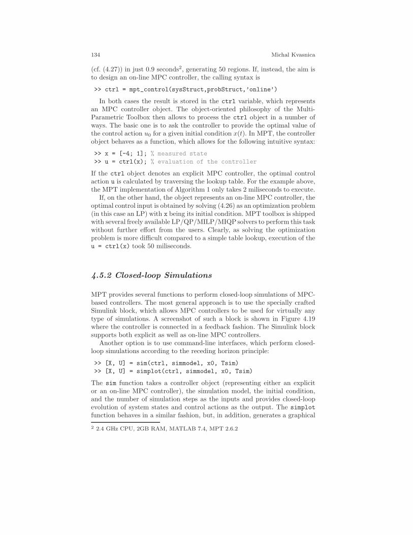
134 Michal Kvasnica
(cf. (4.27)) in just 0.9 seconds2, generating 50 regions. If, instead, the aim isto design an on-line MPC controller, the calling syntax is
>> ctrl = mpt_control(sysStruct,probStruct,’online’)
In both cases the result is stored in the ctrl variable, which representsan MPC controller object. The object-oriented philosophy of the Multi-Parametric Toolbox then allows to process the ctrl object in a number ofways. The basic one is to ask the controller to provide the optimal value ofthe control action u0 for a given initial condition x(t). In MPT, the controllerobject behaves as a function, which allows for the following intuitive syntax:
>> x = [-4; 1]; % measured state
>> u = ctrl(x); % evaluation of the controller
If the ctrl object denotes an explicit MPC controller, the optimal controlaction u is calculated by traversing the lookup table. For the example above,the MPT implementation of Algorithm 1 only takes 2 miliseconds to execute.
If, on the other hand, the object represents an on-line MPC controller, theoptimal control input is obtained by solving (4.26) as an optimization problem(in this case an LP) with x being its initial condition. MPT toolbox is shippedwith several freely available LP/QP/MILP/MIQP solvers to perform this taskwithout further effort from the users. Clearly, as solving the optimizationproblem is more difficult compared to a simple table lookup, execution of theu = ctrl(x) took 50 miliseconds.
4.5.2 Closed-loop Simulations
MPT provides several functions to perform closed-loop simulations of MPC-based controllers. The most general approach is to use the specially craftedSimulink block, which allows MPC controllers to be used for virtually anytype of simulations. A screenshot of such a block is shown in Figure 4.19where the controller is connected in a feedback fashion. The Simulink blocksupports both explicit as well as on-line MPC controllers.
Another option is to use command-line interfaces, which perform closed-loop simulations according to the receding horizon principle:
>> [X, U] = sim(ctrl, simmodel, x0, Tsim)
>> [X, U] = simplot(ctrl, simmodel, x0, Tsim)
The sim function takes a controller object (representing either an explicitor an on-line MPC controller), the simulation model, the initial condition,and the number of simulation steps as the inputs and provides closed-loopevolution of system states and control actions as the output. The simplot
function behaves in a similar fashion, but, in addition, generates a graphical
2 2.4 GHz CPU, 2GB RAM, MATLAB 7.4, MPT 2.6.2
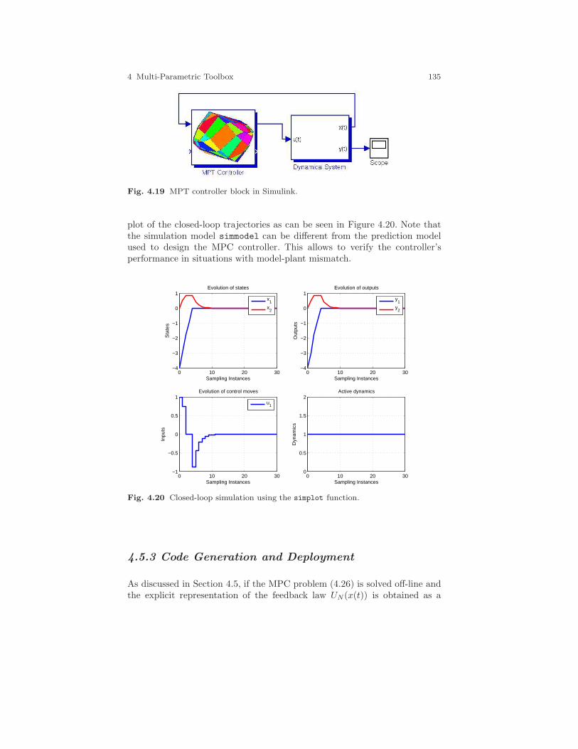
4 Multi-Parametric Toolbox 135
Fig. 4.19 MPT controller block in Simulink.
plot of the closed-loop trajectories as can be seen in Figure 4.20. Note thatthe simulation model simmodel can be different from the prediction modelused to design the MPC controller. This allows to verify the controller’sperformance in situations with model-plant mismatch.
0 10 20 30−4
−3
−2
−1
0
1Evolution of states
Sampling Instances
Sta
tes
x
1
x2
0 10 20 30−4
−3
−2
−1
0
1Evolution of outputs
Sampling Instances
Out
puts
y
1
y2
0 10 20 30−1
−0.5
0
0.5
1Evolution of control moves
Sampling Instances
Inpu
ts
u
1
0 10 20 300
0.5
1
1.5
2Active dynamics
Sampling Instances
Dyn
amic
s
Fig. 4.20 Closed-loop simulation using the simplot function.
4.5.3 Code Generation and Deployment
As discussed in Section 4.5, if the MPC problem (4.26) is solved off-line andthe explicit representation of the feedback law UN(x(t)) is obtained as a
136 Michal Kvasnica
lookup table, the optimal control action can be obtained at each samplinginstant by Algorithm 1. As the algorithm only performs trivial arithmeticoperations, it can be implemented using any high- or low-level programminglanguage. Simplicity of the individual operations also allows the table tobe traversed using low computational power. This makes the approach ofhigh practical relevance when applying MPC to systems with fast dynamicsusing low-cost hardware. To push into this direction, the MPT toolbox canautomatically generate real-time executable C-code version of Algorithm 1.The export can be initiated by calling
>> mpt_exportC(ctrl, ’target_filename’)
The function generates the files target_filename.cand target_filename.hwhich will contain, respectively, the table evaluation code and the table data(the regions Ri and the feedback gains Ki and Li, cf. (4.27)). The code canbe subsequently linked to any application written in the C language.
Another option is to use the Real-Time Workshop (RTW), which is ade-facto standard code generation tool supporting different types of digitalsignal processors and other CPUs. MPT provides a RTW-compatible C-codeimplementation of the Algorithm 1, which makes code generation and de-ployment a single click operation. To use this option, the controller is firstembedded into the Simulink environment using a provided block as shownin Section 4.5.2. The block is subsequently connected to signals from A/Dand D/A converters to close the control loop. Then, one simply clicks onthe respective icon in the Simulink window to initiate RTW, which compilesthe overall control scheme including the lookup table and then automaticallydownloads it to any supported target CPU.
4.5.4 Advanced MPC using MPT and YALMIP
In the previous section we have shown how to formulate, solve, analyze anddeploy MPC controllers using the MPT toolbox. The control design was basedon two main input objects – the sysStruct structure, which contains infor-mation about the system dynamics, and the probStruct structure, whichdefined parameters of the MPC optimization problem (4.26).
Although intuitive and easy to use, the command-line interface outlinedin Section 4.5.1 only allows for basic MPC design. In particular, the MPCproblem to be formulated and solved can only be adjusted by changing theprediction horizon or the penalty matrices in (4.26a). In this section we de-scribe a new addition to the Multi-Parametric Toolbox which allows moreadvanced MPC setups to be formulated easily and with low human effort.
The new framework for advanced model predictive control utilizes theYALMIP package, which is a versatile modeling language for construction ofgeneric optimization problems in MATLAB. The design procedure goes as
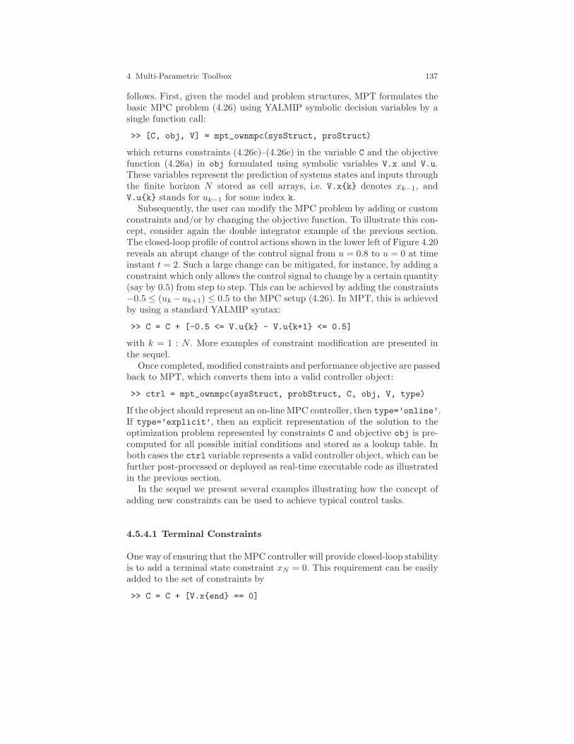
4 Multi-Parametric Toolbox 137
follows. First, given the model and problem structures, MPT formulates thebasic MPC problem (4.26) using YALMIP symbolic decision variables by asingle function call:
>> [C, obj, V] = mpt_ownmpc(sysStruct, proStruct)
which returns constraints (4.26c)–(4.26e) in the variable C and the objectivefunction (4.26a) in obj formulated using symbolic variables V.x and V.u.These variables represent the prediction of systems states and inputs throughthe finite horizon N stored as cell arrays, i.e. V.xk denotes xk−1, andV.uk stands for uk−1 for some index k.
Subsequently, the user can modify the MPC problem by adding or customconstraints and/or by changing the objective function. To illustrate this con-cept, consider again the double integrator example of the previous section.The closed-loop profile of control actions shown in the lower left of Figure 4.20reveals an abrupt change of the control signal from u = 0.8 to u = 0 at timeinstant t = 2. Such a large change can be mitigated, for instance, by adding aconstraint which only allows the control signal to change by a certain quantity(say by 0.5) from step to step. This can be achieved by adding the constraints−0.5 ≤ (uk −uk+1) ≤ 0.5 to the MPC setup (4.26). In MPT, this is achievedby using a standard YALMIP syntax:
>> C = C + [-0.5 <= V.uk - V.uk+1 <= 0.5]
with k = 1 : N . More examples of constraint modification are presented inthe sequel.
Once completed, modified constraints and performance objective are passedback to MPT, which converts them into a valid controller object:
>> ctrl = mpt_ownmpc(sysStruct, probStruct, C, obj, V, type)
If the object should represent an on-line MPC controller, then type=’online’.If type=’explicit’, then an explicit representation of the solution to theoptimization problem represented by constraints C and objective obj is pre-computed for all possible initial conditions and stored as a lookup table. Inboth cases the ctrl variable represents a valid controller object, which can befurther post-processed or deployed as real-time executable code as illustratedin the previous section.
In the sequel we present several examples illustrating how the concept ofadding new constraints can be used to achieve typical control tasks.
4.5.4.1 Terminal Constraints
One way of ensuring that the MPC controller will provide closed-loop stabilityis to add a terminal state constraint xN = 0. This requirement can be easilyadded to the set of constraints by
>> C = C + [V.xend == 0]
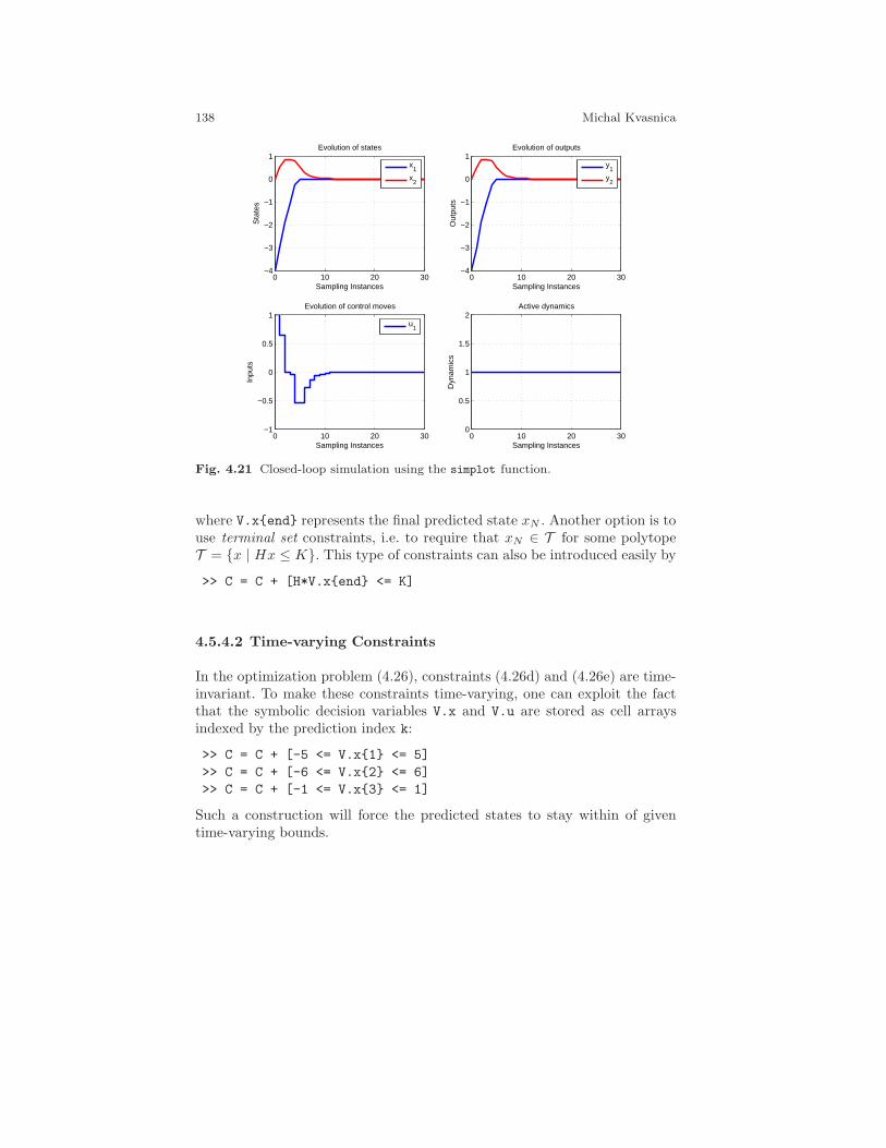
138 Michal Kvasnica
0 10 20 30−4
−3
−2
−1
0
1Evolution of states
Sampling Instances
Sta
tes
x
1
x2
0 10 20 30−4
−3
−2
−1
0
1Evolution of outputs
Sampling Instances
Out
puts
y
1
y2
0 10 20 30−1
−0.5
0
0.5
1Evolution of control moves
Sampling Instances
Inpu
ts
u
1
0 10 20 300
0.5
1
1.5
2Active dynamics
Sampling InstancesD
ynam
ics
Fig. 4.21 Closed-loop simulation using the simplot function.
where V.xend represents the final predicted state xN . Another option is touse terminal set constraints, i.e. to require that xN ∈ T for some polytopeT = x | Hx ≤ K. This type of constraints can also be introduced easily by
>> C = C + [H*V.xend <= K]
4.5.4.2 Time-varying Constraints
In the optimization problem (4.26), constraints (4.26d) and (4.26e) are time-invariant. To make these constraints time-varying, one can exploit the factthat the symbolic decision variables V.x and V.u are stored as cell arraysindexed by the prediction index k:
>> C = C + [-5 <= V.x1 <= 5]
>> C = C + [-6 <= V.x2 <= 6]
>> C = C + [-1 <= V.x3 <= 1]
Such a construction will force the predicted states to stay within of giventime-varying bounds.
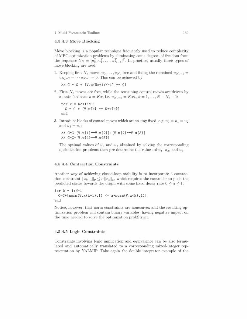
4 Multi-Parametric Toolbox 139
4.5.4.3 Move Blocking
Move blocking is a popular technique frequently used to reduce complexityof MPC optimization problems by eliminating some degrees of freedom fromthe sequence UN = [uT
0 , uT1 , . . . , u
TN−1]
T . In practice, usually three types ofmove blocking are used:
1. Keeping first Nc moves u0, . . . , uNcfree and fixing the remained uNc+1 =
uNc+2 = · · ·uN−1 = 0. This can be achieved by
>> C = C + [V.u(Nc+1:N-1) == 0]
2. First Nc moves are free, while the remaining control moves are driven bya state feedback u = Kx, i.e. uNc+k = Kxk, k = 1, . . . , N −Nc − 1:
for k = Nc+1:N-1
C = C + [V.uk == K*xk]
end
3. Introduce blocks of control moves which are to stay fixed, e.g. u0 = u1 = u2
and u3 = u4:
>> C=C+[V.u1==V.u2]+[V.u2==V.u3]
>> C=C+[V.u4==V.u5]
The optimal values of u0 and u3 obtained by solving the correspondingoptimization problems then pre-determine the values of u1, u2, and u4.
4.5.4.4 Contraction Constraints
Another way of achieving closed-loop stability is to incorporate a contrac-tion constraint ‖xk+1‖p ≤ α‖xk‖p, which requires the controller to push thepredicted states towards the origin with some fixed decay rate 0 ≤ α ≤ 1:
for k = 1:N-1
C=C+[norm(V.xk+1,1) <= a*norm(V.xk,1)]
end
Notice, however, that norm constraints are nonconvex and the resulting op-timization problem will contain binary variables, having negative impact onthe time needed to solve the optimization probStruct.
4.5.4.5 Logic Constraints
Constraints involving logic implication and equivalence can be also formu-lated and automatically translated to a corresponding mixed-integer rep-resentation by YALMIP. Take again the double integrator example of the
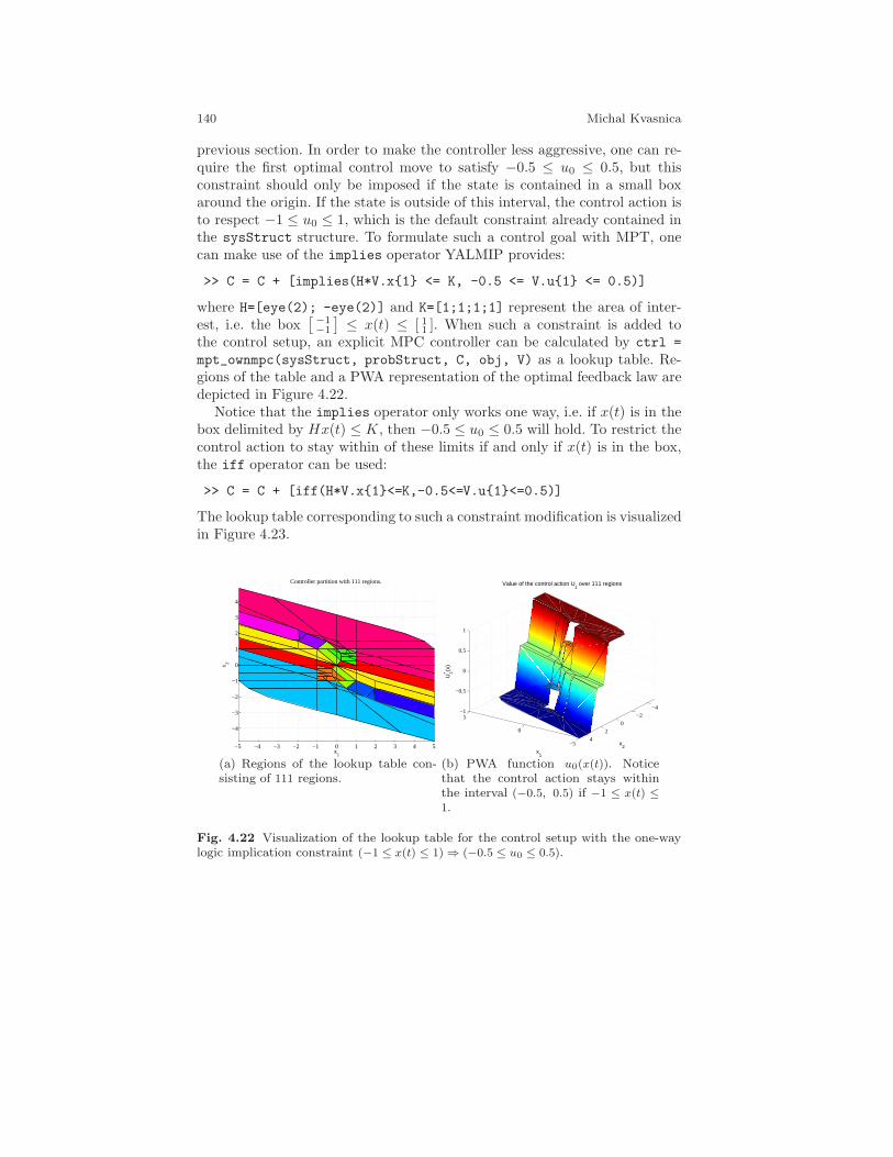
140 Michal Kvasnica
previous section. In order to make the controller less aggressive, one can re-quire the first optimal control move to satisfy −0.5 ≤ u0 ≤ 0.5, but thisconstraint should only be imposed if the state is contained in a small boxaround the origin. If the state is outside of this interval, the control action isto respect −1 ≤ u0 ≤ 1, which is the default constraint already contained inthe sysStruct structure. To formulate such a control goal with MPT, onecan make use of the implies operator YALMIP provides:
>> C = C + [implies(H*V.x1 <= K, -0.5 <= V.u1 <= 0.5)]
where H=[eye(2); -eye(2)] and K=[1;1;1;1] represent the area of inter-est, i.e. the box
[−1−1
]≤ x(t) ≤ [ 11 ]. When such a constraint is added to
the control setup, an explicit MPC controller can be calculated by ctrl =
mpt_ownmpc(sysStruct, probStruct, C, obj, V) as a lookup table. Re-gions of the table and a PWA representation of the optimal feedback law aredepicted in Figure 4.22.
Notice that the implies operator only works one way, i.e. if x(t) is in thebox delimited by Hx(t) ≤ K, then −0.5 ≤ u0 ≤ 0.5 will hold. To restrict thecontrol action to stay within of these limits if and only if x(t) is in the box,the iff operator can be used:
>> C = C + [iff(H*V.x1<=K,-0.5<=V.u1<=0.5)]
The lookup table corresponding to such a constraint modification is visualizedin Figure 4.23.
−5 −4 −3 −2 −1 0 1 2 3 4 5
−4
−3
−2
−1
0
1
2
3
4
x1
x 2
Controller partition with 111 regions.
(a) Regions of the lookup table con-sisting of 111 regions.
−5
0
5
−4−2
02
4
−1
−0.5
0
0.5
1
x2
Value of the control action U1 over 111 regions
x1
U* 1(x
)
(b) PWA function u0(x(t)). Noticethat the control action stays withinthe interval (−0.5, 0.5) if −1 ≤ x(t) ≤1.
Fig. 4.22 Visualization of the lookup table for the control setup with the one-waylogic implication constraint (−1 ≤ x(t) ≤ 1) ⇒ (−0.5 ≤ u0 ≤ 0.5).
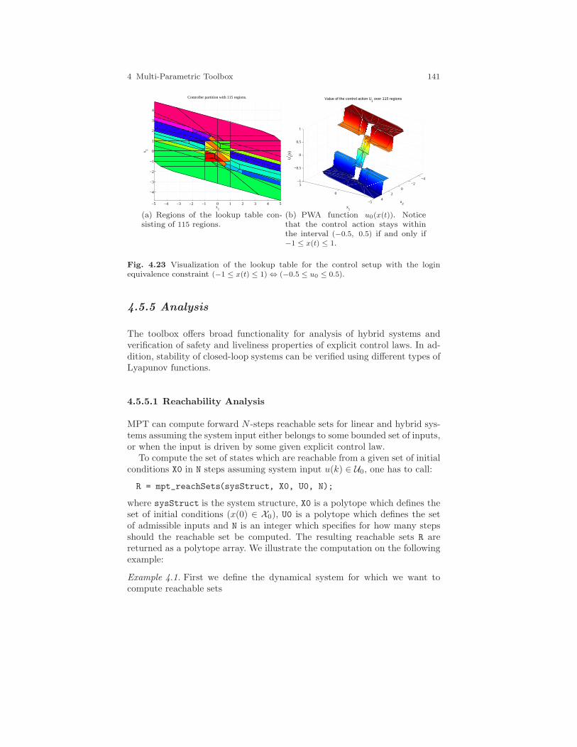
4 Multi-Parametric Toolbox 141
−5 −4 −3 −2 −1 0 1 2 3 4 5
−4
−3
−2
−1
0
1
2
3
4
x1
x 2
Controller partition with 115 regions.
(a) Regions of the lookup table con-sisting of 115 regions.
−5
0
5
−4−2
02
4
−1
−0.5
0
0.5
1
x2
Value of the control action U1 over 115 regions
x1
U* 1(x
)
(b) PWA function u0(x(t)). Noticethat the control action stays withinthe interval (−0.5, 0.5) if and only if−1 ≤ x(t) ≤ 1.
Fig. 4.23 Visualization of the lookup table for the control setup with the loginequivalence constraint (−1 ≤ x(t) ≤ 1) ⇔ (−0.5 ≤ u0 ≤ 0.5).
4.5.5 Analysis
The toolbox offers broad functionality for analysis of hybrid systems andverification of safety and liveliness properties of explicit control laws. In ad-dition, stability of closed-loop systems can be verified using different types ofLyapunov functions.
4.5.5.1 Reachability Analysis
MPT can compute forward N -steps reachable sets for linear and hybrid sys-tems assuming the system input either belongs to some bounded set of inputs,or when the input is driven by some given explicit control law.
To compute the set of states which are reachable from a given set of initialconditions X0 in N steps assuming system input u(k) ∈ U0, one has to call:
R = mpt_reachSets(sysStruct, X0, U0, N);
where sysStruct is the system structure, X0 is a polytope which defines theset of initial conditions (x(0) ∈ X0), U0 is a polytope which defines the setof admissible inputs and N is an integer which specifies for how many stepsshould the reachable set be computed. The resulting reachable sets R arereturned as a polytope array. We illustrate the computation on the followingexample:
Example 4.1. First we define the dynamical system for which we want tocompute reachable sets
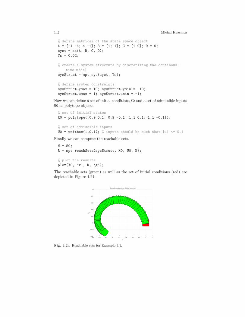
142 Michal Kvasnica
% define matrices of the state-space object
A = [-1 -4; 4 -1]; B = [1; 1]; C = [1 0]; D = 0;
syst = ss(A, B, C, D);
Ts = 0.02;
% create a system structure by discretizing the continous-
time model
sysStruct = mpt_sys(syst, Ts);
% define system constraints
sysStruct.ymax = 10; sysStruct.ymin = -10;
sysStruct.umax = 1; sysStruct.umin = -1;
Now we can define a set of initial conditions X0 and a set of admissible inputsU0 as polytope objects.
% set of initial states
X0 = polytope([0.9 0.1; 0.9 -0.1; 1.1 0.1; 1.1 -0.1]);
% set of admissible inputs
U0 = unitbox(1,0.1); % inputs should be such that |u| <= 0.1
Finally we can compute the reachable sets.
N = 50;
R = mpt_reachSets(sysStruct, X0, U0, N);
% plot the results
plot(X0, ’r’, R, ’g’);
The reachable sets (green) as well as the set of initial conditions (red) aredepicted in Figure 4.24.
−0.6 −0.4 −0.2 0 0.2 0.4 0.6 0.8 1 1.2−0.4
−0.2
0
0.2
0.4
0.6
0.8
1
x1
x 2
Reachable sets (green), set of initial states (red)
Fig. 4.24 Reachable sets for Example 4.1.

4 Multi-Parametric Toolbox 143
To compute reachable sets for linear or hybrid systems whose inputs aredriven by an explicit control law, the following syntax can be used:
R = mpt_reachSets(ctrl, X0, N);
where ctrl is the controller object as generated by mpt_control, X0 is a poly-tope which defines a set of initial conditions (x(0) ∈ X0), and N is an integerwhich specifies for how many steps should the reachable set be computed.The resulting reachable sets R are again returned as polytope array.
Example 4.2. In this example we illustrate the reachability computation onthe double integrator example
% load system and problem parameters
Double_Integrator
% compute explicit controller
ctrl = mpt_control(sysStruct, probStruct);
% define the set of initial conditions
X0 = unitbox(2,1) + [3;0];
% compute the 5-Steps reachable set
N = 5;
R = mpt_reachSets(ctrl, X0, N);
% plot results
plot(ctrl.Pn, ’y’, X0, ’r’, R, ’g’);
The reachable sets (green) as well as the set of initial conditions (red) aredepicted on top of the controller regions (yellow) in Figure 4.25.
−6 −4 −2 0 2 4 6−4
−3
−2
−1
0
1
2
3
4
x1
x 2
Reachable sets (green), set of initial conditions X0 (red), controller regions (yellow)
Fig. 4.25 Reachable sets for Example 4.2.
144 Michal Kvasnica
4.5.5.2 Verification
Reachability computation can be directly extended to answer the followingquestion: Do the states of a dynamical system (whose inputs either belongto some set of admissible inputs, or whose inputs are driven by an explicitcontrol law) enter some set of “unsafe” states in a given number of steps?
Example 4.3. In this example we show how to answer the verification ques-tion for the first case, i.e. system inputs belong to some set of admissibleinputs (u(k) ∈ U0). Although we use a linear system here, exactly the sameprocedure applies to hybrid systems in PWA representation as well.
% define matrices of the state-space object
A = [-1 -4; 4 -1]; B = [1; 1]; C = [1 0]; D = 0;
syst = ss(A, B, C, D);
Ts = 0.02;
% create a system structure by discretizing the continous-
time model
sysStruct = mpt_sys(syst, Ts);
% define system constraints
sysStruct.ymax = 10; sysStruct.ymin = -10;
sysStruct.umax = 1; sysStruct.umin = -1;
% define the set of initial condintions as a polytope object
X0 = polytope([0.9 0.1; 0.9 -0.1; 1.1 0.1; 1.1 -0.1]);
% set of admissible inputs as a polytope object
U0 = unitbox(1,0.1); % inputs should be such that |u| <= 0.1
% set of final states (the ‘‘unsafe’’ states)
Xf = unitbox(2,0.1) + [-0.2; -0.2];
% number of steps
N = 50;
% perform verification
[canreach, Nf] = mpt_verify(sysStruct, X0, Xf, N, U0);
If the system states can reach the set Xf, canreach will be true, otherwisethe function will return false. In case Xf can be reached, the optional secondoutput argument Nf will return the number of steps in which Xf can bereached from X0.
Example 4.4. It is also possible to answer the verification question if the sys-tem inputs are driven by an explicit control law:
4 Multi-Parametric Toolbox 145
% load dynamical system
Double_Integrator
% compute explicit controller
expc = mpt_control(sysStruct, probStruct);
% define set of initial condintions as a polytope object
X0 = unitbox(2,1) + [3;0];
% set of final states (the ‘‘unsafe’’ states)
Xf = unitbox(2,0.1) + [-0.2; -0.2];
% number of steps
N = 10;
% perform verification
[canreach, Nf] = mpt_verify(expc, X0, Xf1, N);
4.5.5.3 Invariant Set Computation
For controllers for which no feasibility guarantee can be given a priori, thefunction mpt_invariantSet can compute an invariant subset of a controller,such that constraints satisfaction is guaranteed for all time.
ctrl_inv = mpt_invariantSet(ctrl)
4.5.5.4 Lyapunov-type Stability Analysis
In terms of stability analysis, MPT offers functions which aim at identifyingquadratic, sum-of-squares, piecewise quadratic, piecewise affine or piecewisepolynomial Lyapunov functions. If such a function is found, it can be usedto show stability of the closed-loop systems even in cases where no suchguarantee can be given a priori based on the design procedure. To computea Lyapunov function, one has to call
ctrl_lyap = mpt_lyapunov(ctrl, lyaptype
where ctrl is an explicit controller and lyaptype is a string parameter whichdefines the type of a Lyapunov function to compute. Allowed values of thesecond parameter are summarized in Table 4.3. Parameters of the Lyapunovfunction, if one exists, will be stored in
lyapfunction = ctrl_lyap.details.lyapunov

146 Michal Kvasnica
lyaptype Type of Lyapunov function’quad’ Common quadratic Lyapunov function’sos’ Common sum-of-squares Lyapunov function’pwa’ Piecewise affine Lyapunov function’pwq’ Piecewise quadratic Lyapunov function’pwp’ Piecewise polynomial Lyapunov function
Table 4.3 Allowed values of the functiontype parameter in mpt_lyapunov.
4.5.5.5 Complexity Reduction
MPT also addresses the issue of complexity reduction of the resulting explicitcontrol laws. As explained in more detail in Section 4.5, the on-line evalua-tion of explicit control laws involves checking which region of the controllercontains a given measured state. Although such an effort is usually small,it can become prohibitive for complex controllers with several thousands oreven more regions. Therefore MPT allows to reduce this complexity by sim-plifying the controller partitions over which the control law is defined. Thissimplification is performed by merging regions which contain the same ex-pression of the control law. By doing so, the number of regions may be greatlyreduced, while maintaining the same performance as the original controller.The results of the merging procedure for a sample explicit controller of ahybrid system is depicted in Figure 4.26.
−10 −8 −6 −4 −2 0 2 4 6 8 10−10
−8
−6
−4
−2
0
2
4
6
8
10
x1
x 2
(a) Regions of an explicit controller beforesimplification (252 regions).
−10 −8 −6 −4 −2 0 2 4 6 8 10−10
−8
−6
−4
−2
0
2
4
6
8
10
x1
x 2
(b) Regions of an explicit controller aftersimplification (39 regions).
Fig. 4.26 Region merging results.
To simplify the representation of a given explicit controller by mergingregions which contain the same control law, one has to call:
ctrl_simple = mpt_simplify(ctrl)
4 Multi-Parametric Toolbox 147
If the function is called as indicated above, a heuristic merging will be used.It is also possible to use optimal merging based on boolean minimization:
ctrl_simple = mpt_simplify(ctrl, ’optimal’)
Note, however, that the optimal merging can be prohibitive for dimensionsabove 2 due to an exponential complexity of the merging procedure Geyer(2005). See clipping method (Kvasnica et al, 2011a) in Textbook and ap-proach based on separation functions (Kvasnica et al, 2011b) in Preprintsfor alternative ways with better convergence properties and larger reductionratio.
4.5.6 System Structure sysStruct
LTI dynamics can be captured by the following linear relations:
x(k + 1) = Ax(k) +Bu(k) (4.28a)
y(k) = Cx(k) +Du(k) (4.28b)
where x(k) ∈ Rnx is the state vector at time instance k, x(k + 1) denotesthe state vector at time k + 1, u(k) ∈ Rnu and y(k) ∈ Rny are values of thecontrol input and system output, respectively. A, B, C and D are matrices ofappropriate dimensions, i.e. A is a nx×nx matrix, dimension of B is nx×nu,C is a ny × nx and D a ny × nu matrix.
Dynamical matrices are stored in the following fields of the system struc-ture:
sysStruct.A = A
sysStruct.B = B
sysStruct.C = C
sysStruct.D = D
Example 4.5. Assume a double integrator dynamics sampled at 1 second:
x(k + 1) =
[1 10 1
]x(k) +
[10.5
]u(k) (4.29a)
y(k) =
[1 00 1
]x(k) +
[00
]u(k) (4.29b)
In MPT, the above described system can be defined as follows:

148 Michal Kvasnica
sysStruct.A = [1 1; 0 1];
sysStruct.B = [1; 0.5];
sysStruct.C = [1 0; 0 1];
sysStruct.D = [0; 0]
4.5.6.1 Import of Models from External Sources
MPT can design control laws for discrete-time constrained linear, switchedlinear and hybrid systems. Hybrid systems can be described in Piecewise-Affine (PWA) or Mixed Logical Dynamical (MLD) representations and anefficient algorithm is provided to switch from one representation to the otherform and vice-versa. To increase user’s comfort, models of dynamical systemscan be imported from various sources:
• Models of hybrid systems generated by the HYSDEL language• MLD structures generated by the function mpt_pwa2mld
• Nonlinear models defined by mpt_nonlinfcn template• State-space and transfer function objects of the Control toolbox,• System identification toolbox objects• MPC toolbox objects
In order to import a dynamical system, one has to call
sysStruct = mpt_sys(object, Ts)
where object can be either a string (in which case the model is importedfrom a corresponding HYSDEL source files), or it can be a variable of one ofthe above mentioned object types. The second input parameter Ts denotessampling time and can be omitted, in which case Ts = 1 is assumed.
Example 4.6. The following code will first define a continuous-time state-space object which is then imported to MPT:
% sampling time
Ts = 1;
% continuous-time model as state-space object
di = ss([1 1; 0 1], [1; 0.5], [1 0; 0 1], [0; 0]);
% import the model and discretize it
sysStruct = mpt_sys(di, Ts);
Note 4.1. If the state-space object is already in discrete-time domain, it isnot necessary to provide the sampling time parameter Ts to mpt_sys. Af-ter importing a model using mpt_sys it is still necessary to define systemconstraints as described previously.
4 Multi-Parametric Toolbox 149
MPT allows to define following types of constraints:
• Min/Max constraints on system outputs• Min/Max constraints on system states• Min/Max constraints on manipulated variables• Min/Max constraints on slew rate of manipulated variables
4.5.6.2 Constraints on System Outputs
Output equation is in general driven by the following relation for PWA sys-tems
y(k) = Cix(k) +Diu(k) + gi (4.30)
and byy(k) = Cx(k) +Du(k) (4.31)
for LTI systems. It is therefore clear that by choice of C = I one can use theseconstraints to restrict system states as well. Min/Max output constraints haveto be given in the following fields of the system structure:
sysStruct.ymax = outmax
sysStruct.ymin = outmin
where outmax and outmin are ny × 1 vectors.
4.5.6.3 Constraints on System States
Constraints on system states are optional and can be defined by
sysStruct.xmax = xmax
sysStruct.xmin = xmin
where xmax and xmin are nx × 1 vectors.
4.5.6.4 Constraints on Manipulated Variables
Goal of each control technique is to design a controller which chooses a propervalue of the manipulated variable in order to achieve the given goal (usuallyto guarantee stability, but other aspects like optimality may also be consid-ered at this point). In most real plants values of manipulated variables arerestricted and these constraints have to be taken into account in controllerdesign procedure. These limitations are usually saturation constraints andcan be captured by min / max bounds. In MPT, constraints on control inputare given in:
sysStruct.umax = inpmax
sysStruct.umin = inpmin
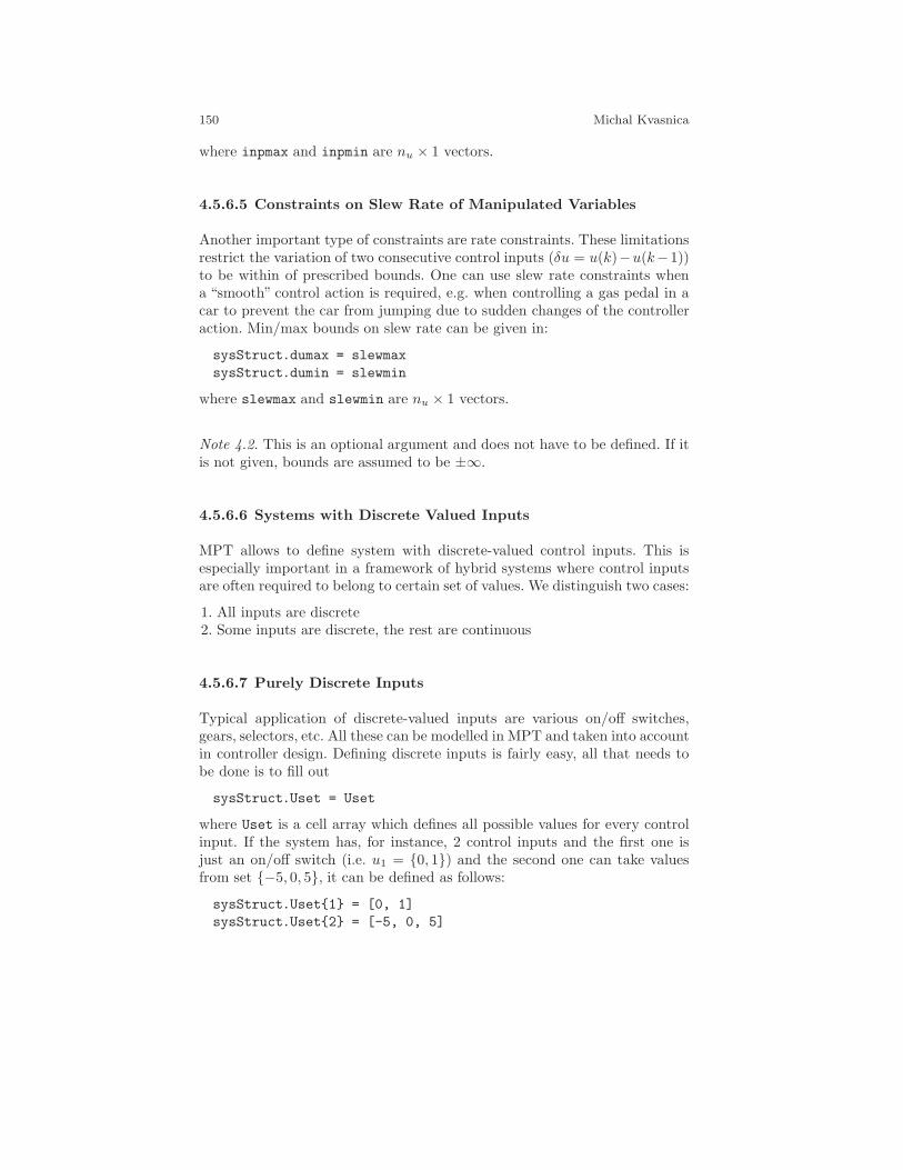
150 Michal Kvasnica
where inpmax and inpmin are nu × 1 vectors.
4.5.6.5 Constraints on Slew Rate of Manipulated Variables
Another important type of constraints are rate constraints. These limitationsrestrict the variation of two consecutive control inputs (δu = u(k)−u(k−1))to be within of prescribed bounds. One can use slew rate constraints whena “smooth” control action is required, e.g. when controlling a gas pedal in acar to prevent the car from jumping due to sudden changes of the controlleraction. Min/max bounds on slew rate can be given in:
sysStruct.dumax = slewmax
sysStruct.dumin = slewmin
where slewmax and slewmin are nu × 1 vectors.
Note 4.2. This is an optional argument and does not have to be defined. If itis not given, bounds are assumed to be ±∞.
4.5.6.6 Systems with Discrete Valued Inputs
MPT allows to define system with discrete-valued control inputs. This isespecially important in a framework of hybrid systems where control inputsare often required to belong to certain set of values. We distinguish two cases:
1. All inputs are discrete2. Some inputs are discrete, the rest are continuous
4.5.6.7 Purely Discrete Inputs
Typical application of discrete-valued inputs are various on/off switches,gears, selectors, etc. All these can be modelled in MPT and taken into accountin controller design. Defining discrete inputs is fairly easy, all that needs tobe done is to fill out
sysStruct.Uset = Uset
where Uset is a cell array which defines all possible values for every controlinput. If the system has, for instance, 2 control inputs and the first one isjust an on/off switch (i.e. u1 = 0, 1) and the second one can take valuesfrom set −5, 0, 5, it can be defined as follows:
sysStruct.Uset1 = [0, 1]
sysStruct.Uset2 = [-5, 0, 5]
4 Multi-Parametric Toolbox 151
where the first line corresponds to u1 and the second to u2. If the system tobe controlled has only one manipulated variable, the cell operator can beomitted, i.e. one could write:
sysStruct.Uset = [0, 1]
The set of inputs doesn’t have to be ordered.
4.5.6.8 Mixed Inputs
Mixed discrete and continuous inputs can be modelled by appropriate choiceof sysStruct.Uset. For each continuous input it is necessary to set the corre-sponding entry to [-Inf Inf], indicating to MPT that this particular inputvariable should be treated as a continuous input. For a system with two ma-nipulated variables, where the first one takes values from a set −2.5, 0, 3.5and the second one is continuous, one would set:
sysStruct.Uset1 = [-2.5, 0, 3.5]
sysStruct.Uset2 = [-Inf Inf]
4.5.6.9 Text Labels
State, input and output variables can be assigned a text label which overridesthe default axis labels in trajectory and partition plotting (xi, ui and yi,respectively). To assign a text label, set the following fields of the systemstructure, e.g. as follows:
sysStruct.xlabels = ’position’, ’speed’;
sysStruct.ulabels = ’force’;
sysStruct.ylabels = ’position’, ’speed’;
Each field is an array of strings corresponding to a given variable. If the userdoes not define any (or some) labels, they will be replaced by default strings(xi, ui and yi). The strings are used once polyhedral partition of the explicitcontroller, or closed-loop (open-loop) trajectories are visualized.
4.5.7 Problem Structure probStruct
Problem structure probStruct is a structure which states an optimizationproblem to be solved by MPT.
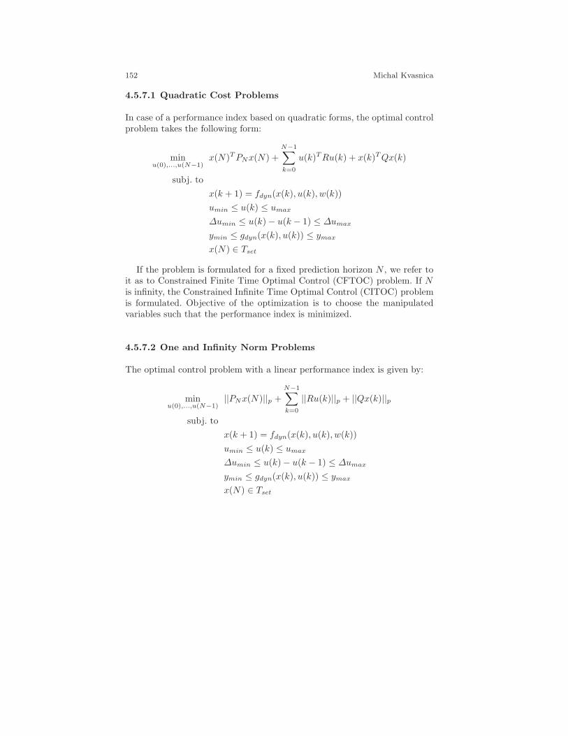
152 Michal Kvasnica
4.5.7.1 Quadratic Cost Problems
In case of a performance index based on quadratic forms, the optimal controlproblem takes the following form:
minu(0),...,u(N−1)
x(N)TPNx(N) +N−1∑
k=0
u(k)TRu(k) + x(k)TQx(k)
subj. to
x(k + 1) = fdyn(x(k), u(k), w(k))
umin ≤ u(k) ≤ umax
∆umin ≤ u(k)− u(k − 1) ≤ ∆umax
ymin ≤ gdyn(x(k), u(k)) ≤ ymax
x(N) ∈ Tset
If the problem is formulated for a fixed prediction horizon N , we refer toit as to Constrained Finite Time Optimal Control (CFTOC) problem. If Nis infinity, the Constrained Infinite Time Optimal Control (CITOC) problemis formulated. Objective of the optimization is to choose the manipulatedvariables such that the performance index is minimized.
4.5.7.2 One and Infinity Norm Problems
The optimal control problem with a linear performance index is given by:
minu(0),...,u(N−1)
||PNx(N)||p +N−1∑
k=0
||Ru(k)||p + ||Qx(k)||p
subj. to
x(k + 1) = fdyn(x(k), u(k), w(k))
umin ≤ u(k) ≤ umax
∆umin ≤ u(k)− u(k − 1) ≤ ∆umax
ymin ≤ gdyn(x(k), u(k)) ≤ ymax
x(N) ∈ Tset
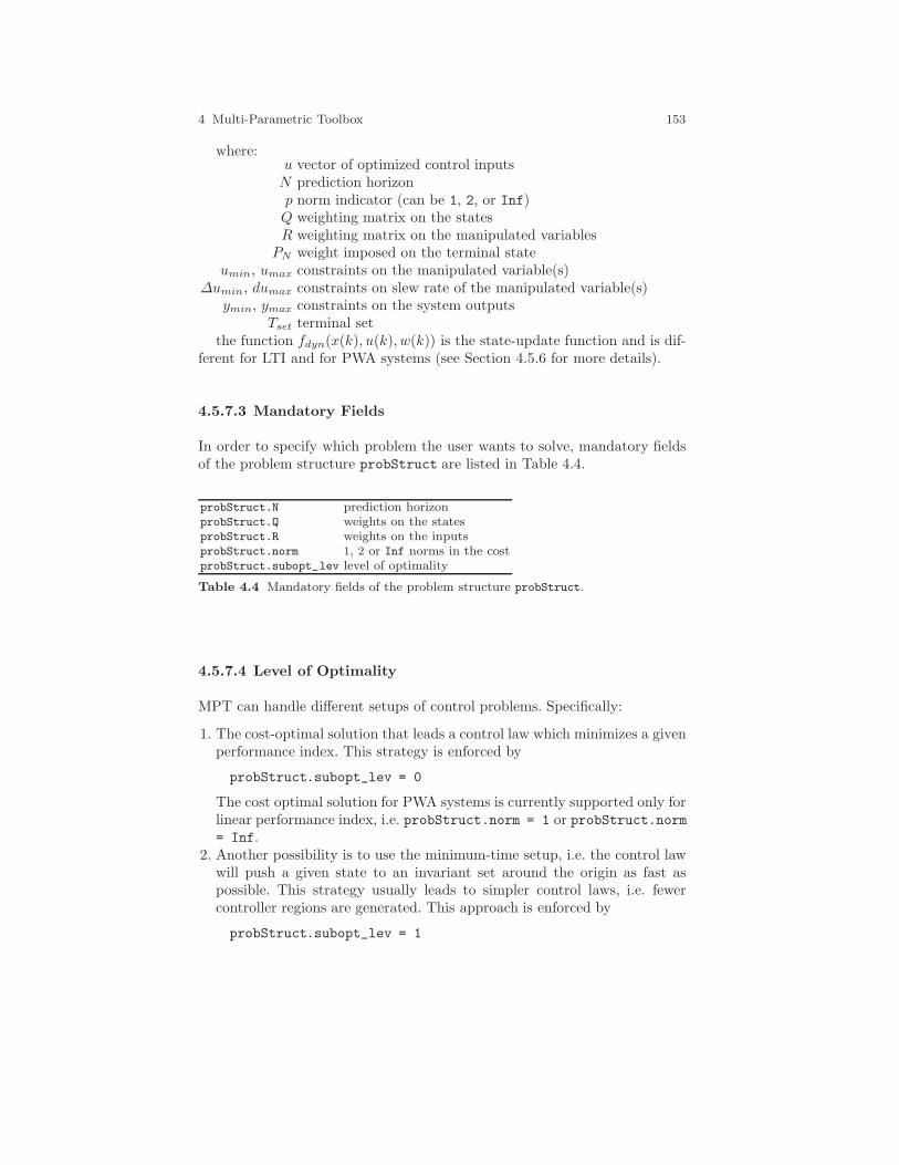
4 Multi-Parametric Toolbox 153
where:u vector of optimized control inputsN prediction horizonp norm indicator (can be 1, 2, or Inf)Q weighting matrix on the statesR weighting matrix on the manipulated variables
PN weight imposed on the terminal stateumin, umax constraints on the manipulated variable(s)
∆umin, dumax constraints on slew rate of the manipulated variable(s)ymin, ymax constraints on the system outputs
Tset terminal setthe function fdyn(x(k), u(k), w(k)) is the state-update function and is dif-
ferent for LTI and for PWA systems (see Section 4.5.6 for more details).
4.5.7.3 Mandatory Fields
In order to specify which problem the user wants to solve, mandatory fieldsof the problem structure probStruct are listed in Table 4.4.
probStruct.N prediction horizonprobStruct.Q weights on the statesprobStruct.R weights on the inputsprobStruct.norm 1, 2 or Inf norms in the costprobStruct.subopt_lev level of optimality
Table 4.4 Mandatory fields of the problem structure probStruct.
4.5.7.4 Level of Optimality
MPT can handle different setups of control problems. Specifically:
1. The cost-optimal solution that leads a control law which minimizes a givenperformance index. This strategy is enforced by
probStruct.subopt_lev = 0
The cost optimal solution for PWA systems is currently supported only forlinear performance index, i.e. probStruct.norm = 1 or probStruct.norm= Inf.
2. Another possibility is to use the minimum-time setup, i.e. the control lawwill push a given state to an invariant set around the origin as fast aspossible. This strategy usually leads to simpler control laws, i.e. fewercontroller regions are generated. This approach is enforced by
probStruct.subopt_lev = 1
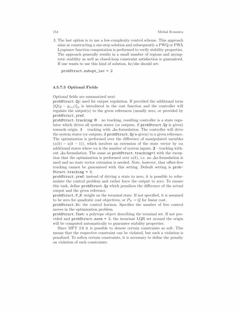
154 Michal Kvasnica
3. The last option is to use a low-complexity control scheme. This approachaims at constructing a one-step solution and subsequently a PWQ or PWALyapunov function computation is performed to verify stability properties.The approach generally results in a small number of regions and asymp-totic stability as well as closed-loop constraint satisfaction is guaranteed.If one wants to use this kind of solution, he/she should set:
probStruct.subopt_lev = 2
4.5.7.5 Optional Fields
Optional fields are summarized next.probStruct.Qy: used for output regulation. If provided the additional term‖Q(y − yref )‖p is introduced in the cost function and the controller willregulate the output(s) to the given references (usually zero, or provided byprobStruct.yref.probStruct.tracking: 0 – no tracking, resulting controller is a state regu-lator which drives all system states (or outputs, if probStruct.Qy is given)towards origin. 1 – tracking with ∆u-formulation. The controller will drivethe system states (or outputs, if probStruct.Qy is given) to a given reference.The optimization is performed over the difference of manipulated variables(u(k) − u(k − 1)), which involves an extension of the state vector by nuadditional states where nu is the number of system inputs. 2 – tracking with-out ∆u-formulation. The same as probStruct.tracking=1 with the excep-tion that the optimization is performed over u(k), i.e. no ∆u-formulation isused and no state vector extension is needed. Note, however, that offset-freetracking cannot be guaranteed with this setting. Default setting is prob-
Struct.tracking = 0.probStruct.yref: instead of driving a state to zero, it is possible to refor-mulate the control problem and rather force the output to zero. To ensurethis task, define probStruct.Qy which penalizes the difference of the actualoutput and the given reference.probStruct.P_N: weight on the terminal state. If not specified, it is assumedto be zero for quadratic cost objectives, or PN = Q for linear cost.probStruct.Nc: the control horizon. Specifies the number of free controlmoves in the optimization problem.probStruct.Tset: a polytope object describing the terminal set. If not pro-vided and probStruct.norm = 2, the invariant LQR set around the originwill be computed automatically to guarantee stability properties.
Since MPT 2.6 it is possible to denote certain constraints as soft. Thismeans that the respective constraint can be violated, but such a violation ispenalized. To soften certain constraints, it is necessary to define the penaltyon violation of such constraints:
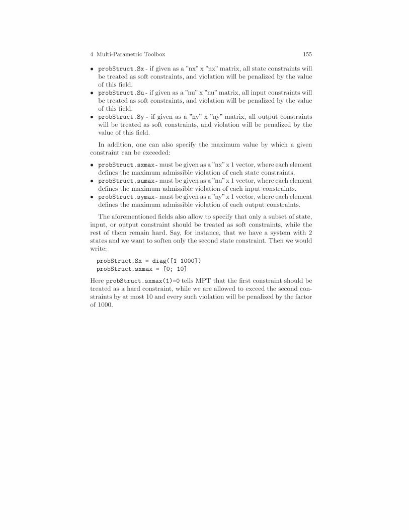
4 Multi-Parametric Toolbox 155
• probStruct.Sx - if given as a ”nx”x ”nx”matrix, all state constraints willbe treated as soft constraints, and violation will be penalized by the valueof this field.
• probStruct.Su - if given as a ”nu”x ”nu”matrix, all input constraints willbe treated as soft constraints, and violation will be penalized by the valueof this field.
• probStruct.Sy - if given as a ”ny” x ”ny” matrix, all output constraintswill be treated as soft constraints, and violation will be penalized by thevalue of this field.
In addition, one can also specify the maximum value by which a givenconstraint can be exceeded:
• probStruct.sxmax - must be given as a ”nx”x 1 vector, where each elementdefines the maximum admissible violation of each state constraints.
• probStruct.sumax - must be given as a ”nu”x 1 vector, where each elementdefines the maximum admissible violation of each input constraints.
• probStruct.symax - must be given as a ”ny”x 1 vector, where each elementdefines the maximum admissible violation of each output constraints.
The aforementioned fields also allow to specify that only a subset of state,input, or output constraint should be treated as soft constraints, while therest of them remain hard. Say, for instance, that we have a system with 2states and we want to soften only the second state constraint. Then we wouldwrite:
probStruct.Sx = diag([1 1000])
probStruct.sxmax = [0; 10]
Here probStruct.sxmax(1)=0 tells MPT that the first constraint should betreated as a hard constraint, while we are allowed to exceed the second con-straints by at most 10 and every such violation will be penalized by the factorof 1000.
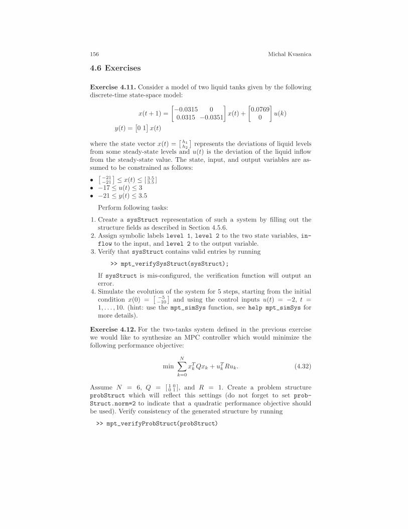
156 Michal Kvasnica
4.6 Exercises
Exercise 4.11. Consider a model of two liquid tanks given by the followingdiscrete-time state-space model:
x(t+ 1) =
[−0.0315 00.0315 −0.0351
]x(t) +
[0.0769
0
]u(k)
y(t) =[0 1
]x(t)
where the state vector x(t) =[h1
h2
]represents the deviations of liquid levels
from some steady-state levels and u(t) is the deviation of the liquid inflowfrom the steady-state value. The state, input, and output variables are as-sumed to be constrained as follows:
•[−21−21
]≤ x(t) ≤ [ 3.53.5 ]
• −17 ≤ u(t) ≤ 3• −21 ≤ y(t) ≤ 3.5
Perform following tasks:
1. Create a sysStruct representation of such a system by filling out thestructure fields as described in Section 4.5.6.
2. Assign symbolic labels level 1, level 2 to the two state variables, in-flow to the input, and level 2 to the output variable.
3. Verify that sysStruct contains valid entries by running
>> mpt_verifySysStruct(sysStruct);
If sysStruct is mis-configured, the verification function will output anerror.
4. Simulate the evolution of the system for 5 steps, starting from the initialcondition x(0) =
[ −5−10
]and using the control inputs u(t) = −2, t =
1, . . . , 10. (hint: use the mpt_simSys function, see help mpt_simSys formore details).
Exercise 4.12. For the two-tanks system defined in the previous exercisewe would like to synthesize an MPC controller which would minimize thefollowing performance objective:
min
N∑
k=0
xTk Qxk + uT
kRuk. (4.32)
Assume N = 6, Q = [ 1 00 1 ], and R = 1. Create a problem structure
probStruct which will reflect this settings (do not forget to set prob-
Struct.norm=2 to indicate that a quadratic performance objective shouldbe used). Verify consistency of the generated structure by running
>> mpt_verifyProbStruct(probStruct)
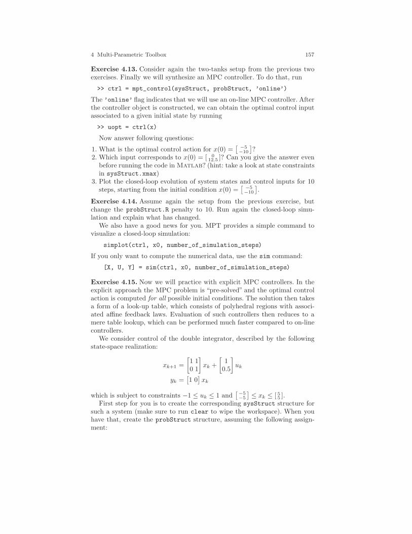
4 Multi-Parametric Toolbox 157
Exercise 4.13. Consider again the two-tanks setup from the previous twoexercises. Finally we will synthesize an MPC controller. To do that, run
>> ctrl = mpt_control(sysStruct, probStruct, ’online’)
The ’online’ flag indicates that we will use an on-line MPC controller. Afterthe controller object is constructed, we can obtain the optimal control inputassociated to a given initial state by running
>> uopt = ctrl(x)
Now answer following questions:
1. What is the optimal control action for x(0) =[ −5−10
]?
2. Which input corresponds to x(0) = [ 012.5 ]? Can you give the answer even
before running the code in Matlab? (hint: take a look at state constraintsin sysStruct.xmax)
3. Plot the closed-loop evolution of system states and control inputs for 10steps, starting from the initial condition x(0) =
[ −5−10
].
Exercise 4.14. Assume again the setup from the previous exercise, butchange the probStruct.R penalty to 10. Run again the closed-loop simu-lation and explain what has changed.
We also have a good news for you. MPT provides a simple command tovisualize a closed-loop simulation:
simplot(ctrl, x0, number_of_simulation_steps)
If you only want to compute the numerical data, use the sim command:
[X, U, Y] = sim(ctrl, x0, number_of_simulation_steps)
Exercise 4.15. Now we will practice with explicit MPC controllers. In theexplicit approach the MPC problem is “pre-solved” and the optimal controlaction is computed for all possible initial conditions. The solution then takesa form of a look-up table, which consists of polyhedral regions with associ-ated affine feedback laws. Evaluation of such controllers then reduces to amere table lookup, which can be performed much faster compared to on-linecontrollers.
We consider control of the double integrator, described by the followingstate-space realization:
xk+1 =
[1 10 1
]xk +
[10.5
]uk
yk =[1 0
]xk
which is subject to constraints −1 ≤ uk ≤ 1 and[−5−5
]≤ xk ≤ [ 55 ].
First step for you is to create the corresponding sysStruct structure forsuch a system (make sure to run clear to wipe the workspace). When youhave that, create the probStruct structure, assuming the following assign-ment:
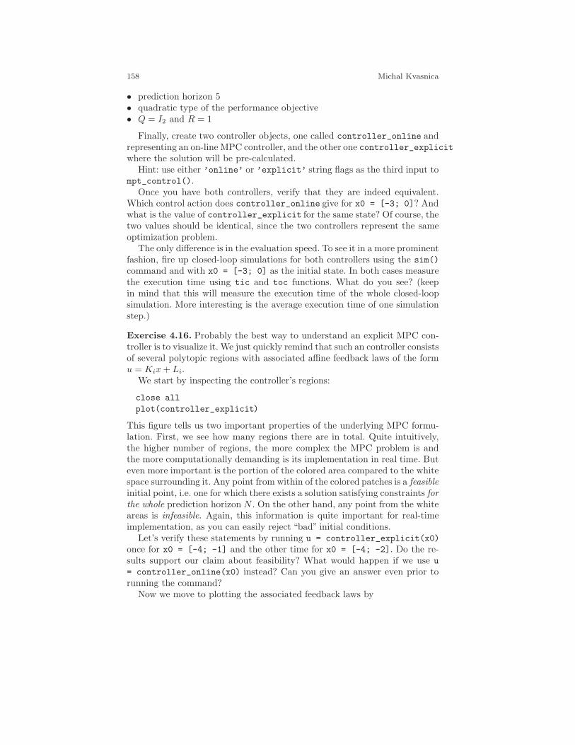
158 Michal Kvasnica
• prediction horizon 5• quadratic type of the performance objective• Q = I2 and R = 1
Finally, create two controller objects, one called controller_online andrepresenting an on-line MPC controller, and the other one controller_explicitwhere the solution will be pre-calculated.
Hint: use either ’online’ or ’explicit’ string flags as the third input tompt_control().
Once you have both controllers, verify that they are indeed equivalent.Which control action does controller_online give for x0 = [-3; 0]? Andwhat is the value of controller_explicit for the same state? Of course, thetwo values should be identical, since the two controllers represent the sameoptimization problem.
The only difference is in the evaluation speed. To see it in a more prominentfashion, fire up closed-loop simulations for both controllers using the sim()
command and with x0 = [-3; 0] as the initial state. In both cases measurethe execution time using tic and toc functions. What do you see? (keepin mind that this will measure the execution time of the whole closed-loopsimulation. More interesting is the average execution time of one simulationstep.)
Exercise 4.16. Probably the best way to understand an explicit MPC con-troller is to visualize it. We just quickly remind that such an controller consistsof several polytopic regions with associated affine feedback laws of the formu = Kix+ Li.
We start by inspecting the controller’s regions:
close all
plot(controller_explicit)
This figure tells us two important properties of the underlying MPC formu-lation. First, we see how many regions there are in total. Quite intuitively,the higher number of regions, the more complex the MPC problem is andthe more computationally demanding is its implementation in real time. Buteven more important is the portion of the colored area compared to the whitespace surrounding it. Any point from within of the colored patches is a feasibleinitial point, i.e. one for which there exists a solution satisfying constraints forthe whole prediction horizon N . On the other hand, any point from the whiteareas is infeasible. Again, this information is quite important for real-timeimplementation, as you can easily reject “bad” initial conditions.
Let’s verify these statements by running u = controller_explicit(x0)
once for x0 = [-4; -1] and the other time for x0 = [-4; -2]. Do the re-sults support our claim about feasibility? What would happen if we use u
= controller_online(x0) instead? Can you give an answer even prior torunning the command?
Now we move to plotting the associated feedback laws by
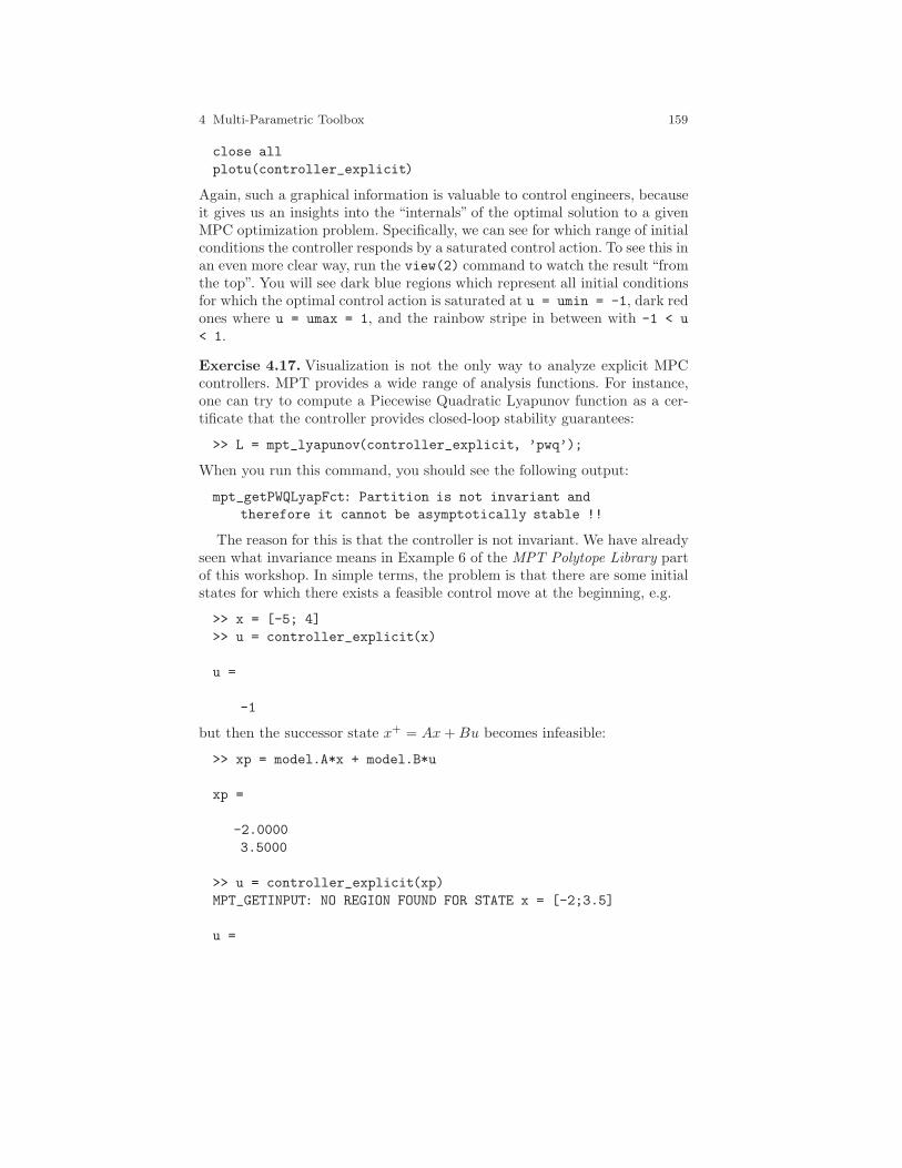
4 Multi-Parametric Toolbox 159
close all
plotu(controller_explicit)
Again, such a graphical information is valuable to control engineers, becauseit gives us an insights into the “internals” of the optimal solution to a givenMPC optimization problem. Specifically, we can see for which range of initialconditions the controller responds by a saturated control action. To see this inan even more clear way, run the view(2) command to watch the result “fromthe top”. You will see dark blue regions which represent all initial conditionsfor which the optimal control action is saturated at u = umin = -1, dark redones where u = umax = 1, and the rainbow stripe in between with -1 < u
< 1.
Exercise 4.17. Visualization is not the only way to analyze explicit MPCcontrollers. MPT provides a wide range of analysis functions. For instance,one can try to compute a Piecewise Quadratic Lyapunov function as a cer-tificate that the controller provides closed-loop stability guarantees:
>> L = mpt_lyapunov(controller_explicit, ’pwq’);
When you run this command, you should see the following output:
mpt_getPWQLyapFct: Partition is not invariant and
therefore it cannot be asymptotically stable !!
The reason for this is that the controller is not invariant. We have alreadyseen what invariance means in Example 6 of the MPT Polytope Library partof this workshop. In simple terms, the problem is that there are some initialstates for which there exists a feasible control move at the beginning, e.g.
>> x = [-5; 4]
>> u = controller_explicit(x)
u =
-1
but then the successor state x+ = Ax+Bu becomes infeasible:
>> xp = model.A*x + model.B*u
xp =
-2.0000
3.5000
>> u = controller_explicit(xp)
MPT_GETINPUT: NO REGION FOUND FOR STATE x = [-2;3.5]
u =
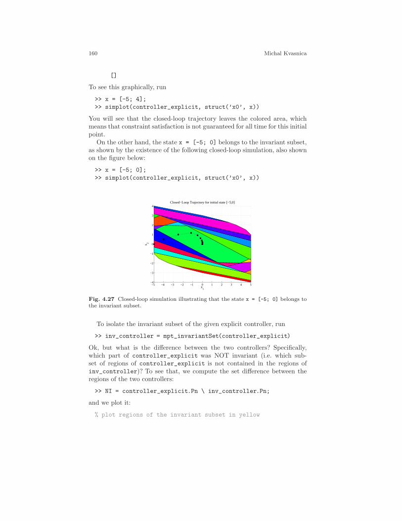
160 Michal Kvasnica
[]
To see this graphically, run
>> x = [-5; 4];
>> simplot(controller_explicit, struct(’x0’, x))
You will see that the closed-loop trajectory leaves the colored area, whichmeans that constraint satisfaction is not guaranteed for all time for this initialpoint.
On the other hand, the state x = [-5; 0] belongs to the invariant subset,as shown by the existence of the following closed-loop simulation, also shownon the figure below:
>> x = [-5; 0];
>> simplot(controller_explicit, struct(’x0’, x))
−5 −4 −3 −2 −1 0 1 2 3 4 5−4
−3
−2
−1
0
1
2
3
4
x1
x 2
Closed−Loop Trajectory for initial state [−5,0]
Fig. 4.27 Closed-loop simulation illustrating that the state x = [-5; 0] belongs tothe invariant subset.
To isolate the invariant subset of the given explicit controller, run
>> inv_controller = mpt_invariantSet(controller_explicit)
Ok, but what is the difference between the two controllers? Specifically,which part of controller_explicit was NOT invariant (i.e. which sub-set of regions of controller_explicit is not contained in the regions ofinv_controller)? To see that, we compute the set difference between theregions of the two controllers:
>> NI = controller_explicit.Pn \ inv_controller.Pn;
and we plot it:
% plot regions of the invariant subset in yellow
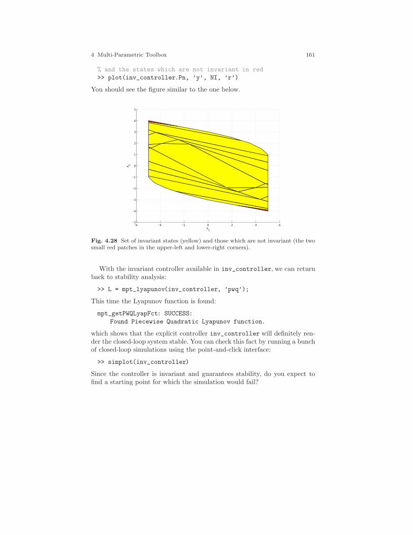
4 Multi-Parametric Toolbox 161
% and the states which are not invariant in red
>> plot(inv_controller.Pn, ’y’, NI, ’r’)
You should see the figure similar to the one below.
−6 −4 −2 0 2 4 6−5
−4
−3
−2
−1
0
1
2
3
4
5
x1
x 2
Fig. 4.28 Set of invariant states (yellow) and those which are not invariant (the twosmall red patches in the upper-left and lower-right corners).
With the invariant controller available in inv_controller, we can returnback to stability analysis:
>> L = mpt_lyapunov(inv_controller, ’pwq’);
This time the Lyapunov function is found:
mpt_getPWQLyapFct: SUCCESS:
Found Piecewise Quadratic Lyapunov function.
which shows that the explicit controller inv_controller will definitely ren-der the closed-loop system stable. You can check this fact by running a bunchof closed-loop simulations using the point-and-click interface:
>> simplot(inv_controller)
Since the controller is invariant and guarantees stability, do you expect tofind a starting point for which the simulation would fail?
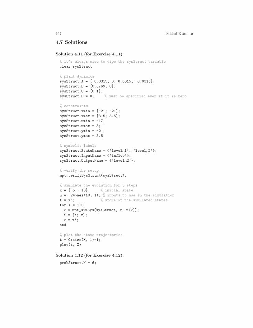
162 Michal Kvasnica
4.7 Solutions
Solution 4.11 (for Exercise 4.11).
% it’s always wise to wipe the sysStruct variable
clear sysStruct
% plant dynamics
sysStruct.A = [-0.0315, 0; 0.0315, -0.0315];
sysStruct.B = [0.0769; 0];
sysStruct.C = [0 1];
sysStruct.D = 0; % must be specified even if it is zero
% constraints
sysStruct.xmin = [-21; -21];
sysStruct.xmax = [3.5; 3.5];
sysStruct.umin = -17;
sysStruct.umax = 3;
sysStruct.ymin = -21;
sysStruct.ymax = 3.5;
% symbolic labels
sysStruct.StateName = ’level 1’, ’level 2’;
sysStruct.InputName = ’inflow’;
sysStruct.OutputName = ’level 2’;
% verify the setup
mpt_verifySysStruct(sysStruct);
% simulate the evolution for 5 steps
x = [-5; -10]; % initial state
u = -2*ones(10, 1); % inputs to use in the simulation
X = x’; % store of the simulated states
for k = 1:5
x = mpt_simSys(sysStruct, x, u(k));
X = [X; x];
x = x’;
end
% plot the state trajectories
t = 0:size(X, 1)-1;
plot(t, X)
Solution 4.12 (for Exercise 4.12).
probStruct.N = 6;
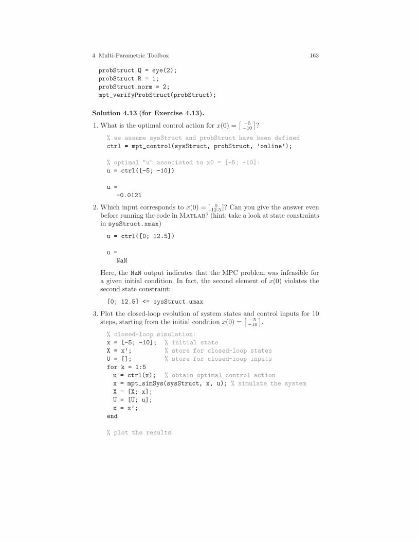
4 Multi-Parametric Toolbox 163
probStruct.Q = eye(2);
probStruct.R = 1;
probStruct.norm = 2;
mpt_verifyProbStruct(probStruct);
Solution 4.13 (for Exercise 4.13).
1. What is the optimal control action for x(0) =[ −5−10
]?
% we assume sysStruct and probStruct have been defined
ctrl = mpt_control(sysStruct, probStruct, ’online’);
% optimal "u" associated to x0 = [-5; -10]:
u = ctrl([-5; -10])
u =
-0.0121
2. Which input corresponds to x(0) = [ 012.5 ]? Can you give the answer even
before running the code in Matlab? (hint: take a look at state constraintsin sysStruct.xmax)
u = ctrl([0; 12.5])
u =
NaN
Here, the NaN output indicates that the MPC problem was infeasible fora given initial condition. In fact, the second element of x(0) violates thesecond state constraint:
[0; 12.5] <= sysStruct.umax
3. Plot the closed-loop evolution of system states and control inputs for 10steps, starting from the initial condition x(0) =
[ −5−10
].
% closed-loop simulation:
x = [-5; -10]; % initial state
X = x’; % store for closed-loop states
U = []; % store for closed-loop inputs
for k = 1:5
u = ctrl(x); % obtain optimal control action
x = mpt_simSys(sysStruct, x, u); % simulate the system
X = [X; x];
U = [U; u];
x = x’;
end
% plot the results
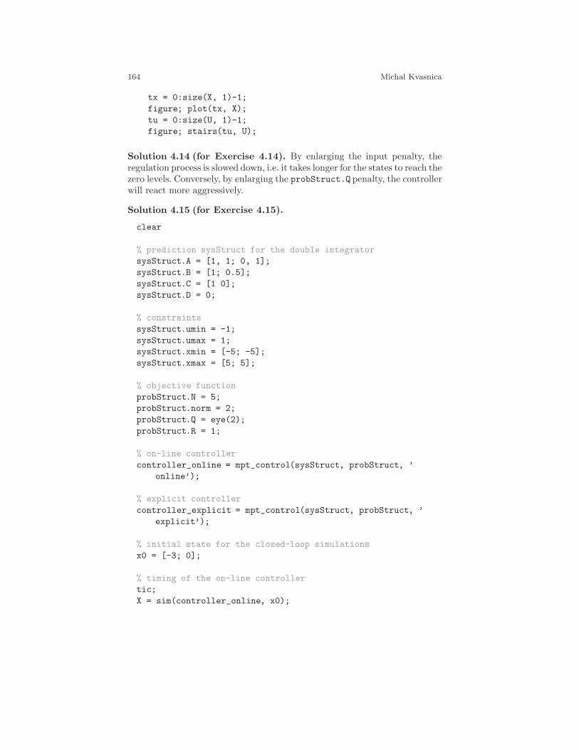
164 Michal Kvasnica
tx = 0:size(X, 1)-1;
figure; plot(tx, X);
tu = 0:size(U, 1)-1;
figure; stairs(tu, U);
Solution 4.14 (for Exercise 4.14). By enlarging the input penalty, theregulation process is slowed down, i.e. it takes longer for the states to reach thezero levels. Conversely, by enlarging the probStruct.Q penalty, the controllerwill react more aggressively.
Solution 4.15 (for Exercise 4.15).
clear
% prediction sysStruct for the double integrator
sysStruct.A = [1, 1; 0, 1];
sysStruct.B = [1; 0.5];
sysStruct.C = [1 0];
sysStruct.D = 0;
% constraints
sysStruct.umin = -1;
sysStruct.umax = 1;
sysStruct.xmin = [-5; -5];
sysStruct.xmax = [5; 5];
% objective function
probStruct.N = 5;
probStruct.norm = 2;
probStruct.Q = eye(2);
probStruct.R = 1;
% on-line controller
controller_online = mpt_control(sysStruct, probStruct, ’
online’);
% explicit controller
controller_explicit = mpt_control(sysStruct, probStruct, ’
explicit’);
% initial state for the closed-loop simulations
x0 = [-3; 0];
% timing of the on-line controller
tic;
X = sim(controller_online, x0);

4 Multi-Parametric Toolbox 165
t = toc; t/size(X, 1)
% timing of the explicit controller
tic;
X = sim(controller_explicit, x0);
t = toc; t/size(X, 1)
Solution 4.16 (for Exercise 4.16).
% run ex_2 to load all necessary data
close all
% plot the controller regions
plot(controller_explicit)
% plot the two initial conditions of interest
x1 = [-4; -1];
x2 = [-4; -2];
hold on
plot(x1(1), x1(2), ’kx’, x2(1), x2(2), ’ko’, ’markersize’,
12);
% optimal control action associated to x1
%
% since x1 is contained in one of the regions,
% we expect a feasible answer
u = controller_explicit(x1)
% check that x1 is indeed in one of the regions
isinside(controller_explicit.Pn, x1)
% optimal control action associated to x2
%
% since x2 is outside of the colored area,
% there should be no control action associated
% to this state, in which case u = []
u = controller_explicit(x2)
% check that x2 is indeed outside of the regions
isinside(controller_explicit.Pn, x2)
% now plot the feedback laws
close all
plotu(controller_explicit)
% rotate the graph manually to inspect it
166 Michal Kvasnica
% finally, look at it from the top
view(2)
Acknowledgements The authors are pleased to acknowledge the financial supportof the Scientific Grant Agency of the Slovak Republic under the grants 1/0071/09 and1/0537/10 and of the Slovak Research and Development Agency under the contractsNo. VV-0029-07 and No. LPP-0092-07. It is also supported by a grant No. NIL-I-007-d from Iceland, Liechtenstein and Norway through the EEA Financial Mechanismand the Norwegian Financial Mechanism.
References
Borrelli F (2003) Constrained Optimal Control Of Linear And Hybrid Systems, Lec-ture Notes in Control and Information Sciences, vol 290. Springer
Geyer T (2005) Low Complexity Model Predictive Control in Power Electronics andPower Systems. Dr. sc. thesis, ETH Zurich, Zurich, Switzerland, available fromhttp://control.ee.ethz.ch/index.cgi?page=publications;action=details;id=2124
Kvasnica M, Fikar M, Cirka L’, Herceg M (2011a) Complexity reduction in explicitmodel predictive control. In: Huba M, Skogestad S, Fikar M, Hovd M, JohansenTA, Rohal’-Ilkiv B (eds) Selected Topics on Constrained and Nonlinear Control.Textbook, STU Bratislava – NTNU Trondheim, pp 241–288
Kvasnica M, Rauova I, Fikar M (2011b) Separation functions used in simplificationof explicit mpc feedback laws. In: Huba M, Skogestad S, Fikar M, Hovd M, Jo-hansen TA, Rohal’-Ilkiv B (eds) Preprints of the NIL workshop: Selected Topicson Constrained and Nonlinear Control, STU Bratislava – NTNU Trondheim, pp48–53

4 Multi-Parametric Toolbox 167
Comments – Remarks

168 Michal Kvasnica
Comments – Remarks

4 Multi-Parametric Toolbox 169
Comments – Remarks

170 Michal Kvasnica
Comments – Remarks
Chapter 5
Implementation of MPC Techniques toReal Mechatronic Systems
Gergely Takacs and Tomas Poloni and Boris Rohal’-Ilkiv and PeterSimoncic and Marek Honek and Matus Kopacka and Jozef Csambal andSlavomır Wojnar
Abstract This chapter is focused on the implementation details of model pre-dictive control for mechatronic systems with fast dynamics. From the very
Gergely TakacsInstitute of Measurement, Automation and Informatics, Faculty of Mechanical Engi-neering, Slovak University of Technology in Bratislava, e-mail: [email protected]
Tomas PoloniInstitute of Measurement, Automation and Informatics, Faculty of Mechanical Engi-neering, Slovak University of Technology in Bratislava, e-mail: [email protected]
Boris Rohal’-IlkivInstitute of Measurement, Automation and Informatics, Faculty of Mechanical En-gineering, Slovak University of Technology in Bratislava, e-mail: [email protected]
Peter SimoncicInstitute of Measurement, Automation and Informatics, Faculty of Mechanical Engi-neering, Slovak University of Technology in Bratislava, e-mail: [email protected]
Marek HonekInstitute of Measurement, Automation and Informatics, Faculty of Mechanical Engi-neering, Slovak University of Technology in Bratislava, e-mail: [email protected]
Matus KopackaInstitute of Measurement, Automation and Informatics, Faculty of Mechanical Engi-neering, Slovak University of Technology in Bratislava, e-mail: [email protected]
Jozef CsambalInstitute of Measurement, Automation and Informatics, Faculty of Mechanical Engi-neering, Slovak University of Technology in Bratislava, e-mail: [email protected]
Slavomır WojnarInstitute of Measurement, Automation and Informatics, Faculty of Mechanical En-gineering, Slovak University of Technology in Bratislava, e-mail: [email protected]
171
172 Gergely Takacs et al
wide application possibilities of MPC and the numerous examples of mecha-tronic systems, two real-life laboratory examples have been selected. Firstan active vibration attenuation system is discussed, with numerous hardwareimplementation details. This is then followed by a detailed discussion of theimplementation of three very different stabilizing MPC approaches: tradi-tional quadratic programming based MPC, pre-computed explicit MPC anda sub-optimal approach called Newton-Raphson’s MPC. Details are given onsoftware and code implementation using coding examples in the Matlab andC programming environment. The next section of this chapter deals with avery different practical example: a spark ignition engine example. This sectionwill introduce the details of a full laboratory setup, hardware implementationdetails and practical issues regarding the use of MPC for the real-time controlof air-fuel ratio in automotive engines.
5.1 Introduction
The merits of well designed control algorithms have been long recognized bythe industry, where a performance improvement of a fraction point leads tosignificantly increased revenue or decreased production cost.
Performance is not the only criterion to judge the qualities of a controlstrategy. Every real actuator and process has inherent physical limits, whichare to be constrained in order to preserve safety, further influence productionoutput or to safeguard equipment. As claimed by Rossiter (2003), the onlycontrol method capable of handling process constraints on an algorithmiclevel is model predictive control (MPC). MPC has been used for decades inapplications, where sampling rates are in the order of several minutes or evenhours: for example in the petrochemical industry. Now the situation turnsto applications with very short sampling periods in orders of millisecondsmainly in mechatronic systems.
This chapter contributes to experimental implementation and real-timeverification of chosen efficient MPC techniques applied for control of fastmechatronic systems, namely laboratory vibration system (subsection 5.2)and internal combustion engine (subsection 5.3).
The section 5.2 discusses the implementation properties of three differ-ent MPC approaches on an experimental laboratory model. This device isbasically a simple lightly damped mechanical structure. The algorithms con-sidered here include the traditional infinite horizon dual-mode quadratic pro-gramming based MPC (QPMPC), pre-computed optimal multi-parametricMPC (MPMPC) and the efficient albeit sub-optimal Newton-Raphson’s MPC(NRMPC).
The control of automotive internal combustion engines is one of most com-plex control problems due to nonlinearities and variable time delays. This isreflected in the time variability of the model parameters in different regions
5 Implementation of MPC Techniques to Real Mechatronic Systems 173
of the engine operating space. The section 5.3 analyzes the practical aspectsof real-time implementation of a multi-model MPC technique to cope withthe problem of nonlinearities and variable time delays in controlling of the SIengine air-fuel ratio.
In both sections the main practical software and hardware aspects of thesuggested real-time solutions are discussed in details.
5.2 Implementation of Various MPC Methods for theVibration Control of Lightly Damped Cantilevers
5.2.1 Introduction
The algorithmic support of active vibration suppression applications is usu-ally limited to simple positive position feedback (PPF) or for example strain-rate feedback (SRF) control (Song et al, 2002). Other essential strategiesinclude PID or linear-quadratic (LQ) control (Preumont, 2002). Because ofthe simplicity of these approaches, no issues regarding computational imple-mentability arise. Even though these control schemes are often sufficient incertain applications, the advantages of MPC cannot be overlooked in vibra-tion damping.
Unfortunately the fast dynamics of vibration attenuation systems requirevery short sampling times, which limit the use of computationally intensiveon-line calculations usually associated with MPC. Traditional quadratic pro-gramming based MPC (QPMPC) has been successfully implemented by Willset al (2008), where the problems raised by the fast sampling were tackled byimplementing a machine code optimized quadratic programming solver ona specialized hardware. While this algorithm handles process constraints, itfails to address the important consequences of stability and constraint feasi-bility.
The stability and constraint feasibility of model predictive control algo-rithms may be guaranteed through the deployment of terminal constraints(Maciejowski, 2002). This unfortunately reduces the range in which the con-trol algorithm may operate, by assigning a region of attraction of all feasibleinitial conditions in the state-space. Amongst others, the size of this regionis dependent on the prediction horizon.
Clamped cantilever beams actuated by piezoelectric strips are a very spe-cial case in the eye of the control engineer. Model predictive control withguaranteed constraint stability and feasibility applied on such and similarsystems raises not only questions associated with algorithm speed but alsowith minimal useful prediction horizon length. Due to the stability require-ment, the useful range the stable MPC controller can operate is severely lim-
174 Gergely Takacs et al
ited, calling for extremely long prediction horizons (Takacs and Rohal’-Ilkiv,2009).
This is partly caused by the large relative deflections compared to the max-imal possible control effort by the piezoelectric actuators, and short samplingtimes. Optimization of prediction dynamics introduced by Cannon and Kou-varitakis (2005) offers a remedy to this problem, as it maximizes the regionof attraction which defines the useful controller range, however this idea isexecuted for for a computationally efficient albeit sub-optimal MPC approachcalled Newton-Raphson’s MPC.
This subsection describes the practical implementation of different MPCmethods onto systems of active vibration control with under-damped dynam-ics. Three MPC methods are introduced here:
• traditional dual-mode quadratic-programming basedMPC (QPMPC) withstability and feasibility guarantees
• a computationally efficient sub-optimal control strategy introduced byKouvaritakis et al (2000), Kouvaritakis et al (2002) and Cannon and Kou-varitakis (2005), called Newton-Raphson MPC (NRMPC)
• and finally an optimal multi-parametric programming based MPC ap-proach (MPMPC)
This section places focus on practical implementation details, while sug-gesting the simplest possible solutions. Therefore no customized on-linequadratic programming solvers or algorithms of multi-parametric program-ming are discussed here. All methods will be implemented in Matlab/Simulink,if possible using off the shelf solutions for off and on-line solvers. Typicallythe problem setup will be carried out in Matlab, while the on-line problemis running on an xPC Target platform system. We will begin our discussionwith introducing the experimental system used as an example.
5.2.2 Brief Description of the Experimental Hardware
A clamped cantilever beam may represent many real life under-damped flex-ible structures, such as helicopter rotor beams, antenna masts, manipulatingarms and solar panels on space structures. The experimental setup consideredas an example to demonstrate different MPC implementations may representthe vibration attenuation of any of the aforementioned physical systems.
The aim of the MPC based vibration control system is to minimize beamtip vibrations, while respecting constraints set by the maximal allowable volt-age levels on the piezoelectric patches. Since piezoelectric materials are proneto depolarization, maximal voltage input levels are set. Additional require-ments placed on the control system are the need for guaranteed stability andconstraint feasibility.
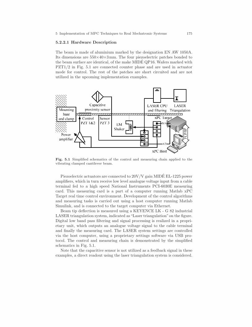
5 Implementation of MPC Techniques to Real Mechatronic Systems 175
5.2.2.1 Hardware Description
The beam is made of aluminium marked by the designation EN AW 1050A.Its dimensions are 550×40×3mm. The four piezoelectric patches bonded tothe beam surface are identical, of the make MIDE QP16. Wafers marked withPZT1/2 in Fig. 5.1 are connected counter phase and are used in actuatormode for control. The rest of the patches are short circuited and are notutilized in the upcoming implementation examples.
Fig. 5.1 Simplified schematics of the control and measuring chain applied to thevibrating clamped cantilever beam.
Piezoelectric actuators are connected to 20V/V gain MIDE EL-1225 poweramplifiers, which in turn receive low level analogue voltage input from a cableterminal fed to a high speed National Instruments PCI-6030E measuringcard. This measuring card is a part of a computer running Matlab xPCTarget real time control environment. Development of the control algorithmsand measuring tasks is carried out using a host computer running MatlabSimulink, and is connected to the target computer via Ethernet.
Beam tip deflection is measured using a KEYENCE LK - G 82 industrialLASER triangulation system, indicated as“Laser triangulation”on the figure.Digital low band pass filtering and signal processing is realized in a propri-etary unit, which outputs an analogue voltage signal to the cable terminaland finally the measuring card. The LASER system settings are controlledvia the host computer, using a proprietary settings software via USB pro-tocol. The control and measuring chain is demonstrated by the simplifiedschematics in Fig. 5.1.
Note that the capacitive sensor is not utilized as a feedback signal in theseexamples, a direct readout using the laser triangulation system is considered.
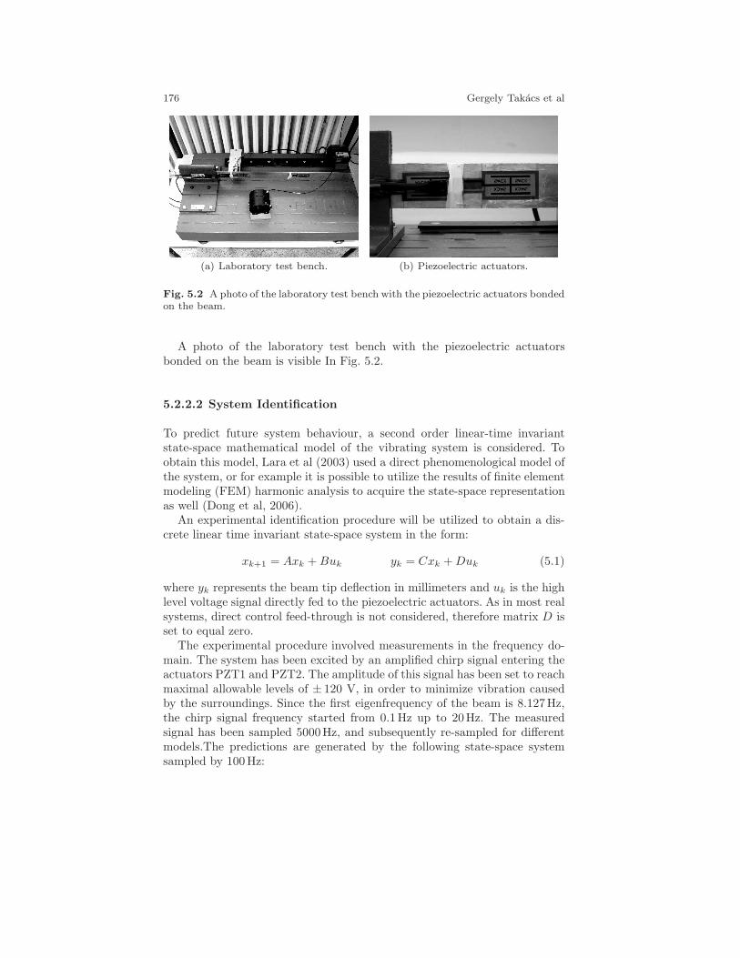
176 Gergely Takacs et al
(a) Laboratory test bench. (b) Piezoelectric actuators.
Fig. 5.2 A photo of the laboratory test bench with the piezoelectric actuators bondedon the beam.
A photo of the laboratory test bench with the piezoelectric actuatorsbonded on the beam is visible In Fig. 5.2.
5.2.2.2 System Identification
To predict future system behaviour, a second order linear-time invariantstate-space mathematical model of the vibrating system is considered. Toobtain this model, Lara et al (2003) used a direct phenomenological model ofthe system, or for example it is possible to utilize the results of finite elementmodeling (FEM) harmonic analysis to acquire the state-space representationas well (Dong et al, 2006).
An experimental identification procedure will be utilized to obtain a dis-crete linear time invariant state-space system in the form:
xk+1 = Axk +Buk yk = Cxk +Duk (5.1)
where yk represents the beam tip deflection in millimeters and uk is the highlevel voltage signal directly fed to the piezoelectric actuators. As in most realsystems, direct control feed-through is not considered, therefore matrix D isset to equal zero.
The experimental procedure involved measurements in the frequency do-main. The system has been excited by an amplified chirp signal entering theactuators PZT1 and PZT2. The amplitude of this signal has been set to reachmaximal allowable levels of ± 120 V, in order to minimize vibration causedby the surroundings. Since the first eigenfrequency of the beam is 8.127Hz,the chirp signal frequency started from 0.1Hz up to 20Hz. The measuredsignal has been sampled 5000Hz, and subsequently re-sampled for differentmodels.The predictions are generated by the following state-space systemsampled by 100Hz:
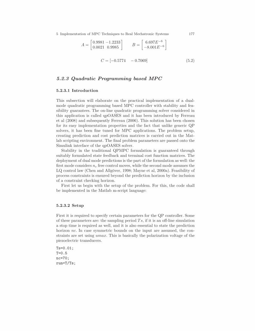
5 Implementation of MPC Techniques to Real Mechatronic Systems 177
A =
[0.9981 −1.22330.0021 0.9985
]B =
[6.697E−6
−8.001E−6
]
C = [−0.5774 − 0.7069] (5.2)
5.2.3 Quadratic Programming based MPC
5.2.3.1 Introduction
This subsection will elaborate on the practical implementation of a dual-mode quadratic programming based MPC controller with stability and fea-sibility guarantees. The on-line quadratic programming solver considered inthis application is called qpOASES and it has been introduced by Ferreauet al (2008) and subsequently Ferreau (2006). This solution has been chosenfor its easy implementation properties and the fact that unlike generic QPsolvers, it has been fine tuned for MPC applications. The problem setup,creating prediction and cost prediction matrices is carried out in the Mat-lab scripting environment. The final problem parameters are passed onto theSimulink interface of the qpOASES solver.
Stability in the traditional QPMPC formulation is guaranteed throughsuitably formulated state feedback and terminal cost function matrices. Thedeployment of dual mode predictions is the part of the formulation as well: thefirst mode considers nc free control moves, while the second mode assumes theLQ control law (Chen and Allgover, 1998; Mayne et al, 2000a). Feasibility ofprocess constraints is ensured beyond the prediction horizon by the inclusionof a constraint checking horizon.
First let us begin with the setup of the problem. For this, the code shallbe implemented in the Matlab m-script language:
5.2.3.2 Setup
First it is required to specify certain parameters for the QP controller. Someof these parameters are: the sampling period Ts, if it is an off-line simulationa stop time is required as well, and it is also essential to state the predictionhorizon nc. In case symmetric bounds on the input are assumed, the con-straints are set using umax. This is basically the polarization voltage of thepiezoelectric transducers.
Ts=0.01;
T=0.5
nc=70;
run=T/Ts;
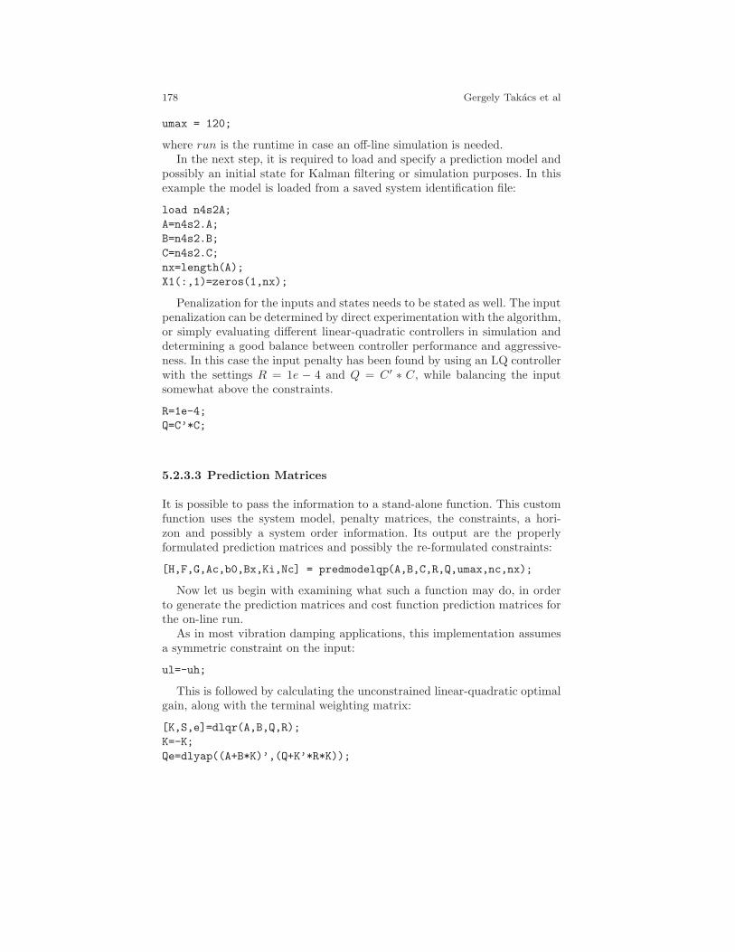
178 Gergely Takacs et al
umax = 120;
where run is the runtime in case an off-line simulation is needed.In the next step, it is required to load and specify a prediction model and
possibly an initial state for Kalman filtering or simulation purposes. In thisexample the model is loaded from a saved system identification file:
load n4s2A;
A=n4s2.A;
B=n4s2.B;
C=n4s2.C;
nx=length(A);
X1(:,1)=zeros(1,nx);
Penalization for the inputs and states needs to be stated as well. The inputpenalization can be determined by direct experimentation with the algorithm,or simply evaluating different linear-quadratic controllers in simulation anddetermining a good balance between controller performance and aggressive-ness. In this case the input penalty has been found by using an LQ controllerwith the settings R = 1e − 4 and Q = C′ ∗ C, while balancing the inputsomewhat above the constraints.
R=1e-4;
Q=C’*C;
5.2.3.3 Prediction Matrices
It is possible to pass the information to a stand-alone function. This customfunction uses the system model, penalty matrices, the constraints, a hori-zon and possibly a system order information. Its output are the properlyformulated prediction matrices and possibly the re-formulated constraints:
[H,F,G,Ac,b0,Bx,Ki,Nc] = predmodelqp(A,B,C,R,Q,umax,nc,nx);
Now let us begin with examining what such a function may do, in orderto generate the prediction matrices and cost function prediction matrices forthe on-line run.
As in most vibration damping applications, this implementation assumesa symmetric constraint on the input:
ul=-uh;
This is followed by calculating the unconstrained linear-quadratic optimalgain, along with the terminal weighting matrix:
[K,S,e]=dlqr(A,B,Q,R);
K=-K;
Qe=dlyap((A+B*K)’,(Q+K’*R*K));
5 Implementation of MPC Techniques to Real Mechatronic Systems 179
The forced and free state prediction matrices are calculated through a setof nested loops according to the following script:
M2=zeros(nc*nx);
for n=1:nc;
M1(n*nx-nx+1:n*nx,:)=[(A^n)];
for na=0:nx:(nc*nx); %na=0:nx:(nc*nx)
m2(nx*(n-1)+(na+1):nx*(n-1)+(na+nx),n)=[(A^(na/nx))*B];
end;
end;
M2=m2(1:nx*nc,:);
where several other possible solutions may exist. These solutions can be equiv-alently good, and while their runtime may differ this should not be an issuein an off-line problem setup process.
The last n rows of the matrices M1 and M2 are also selected:
M1l=M1(nx*nc-(nx-1):nx*nc,:);
M2l=M2(nx*nc-(nx-1):nx*nc,:);
The next step is to create the cost prediction matrices. One has to beginwith initialization:
H1=0;
F1=0;
G1=A^0*Q;
This is then followed by creating the cost prediction matrices H , F and G- first by running the following loop to get partial results:
for i=0:nc-2
H1t=M2(1+i*nx:i*nx+nx,:)’*Q*M2(1+i*nx:i*nx+nx,:);
H1=H1+H1t;
F1t=M2(1+i*nx:i*nx+nx,:)’*Q*M1(1+i*nx:i*nx+nx,:);
F1=F1+F1t;
G1t=M1(1+i*nx:i*nx+nx,:)’*Q*M1(1+i*nx:i*nx+nx,:);
G1=G1+G1t;
end
And finally assembling cost prediction matrices H , F and G:
H=H1+M2(1+(nc-1)*nx:(nc-1)*nx+nx,:)’*Qe*M2(1+(nc-1)*nx:(nc-1)*
nx+nx,:)+R*eye(nc);
F=F1+M2(1+(nc-1)*nx:(nc-1)*nx+nx,:)’*Qe*M1(1+(nc-1)*nx:(nc-1)*
nx+nx,:);
G=G1+M1(1+(nc-1)*nx:(nc-1)*nx+nx,:)’*Qe*M1(1+(nc-1)*nx:(nc-1)*
nx+nx,:);
To ensure feasibility and stability beyond the prediction horizon, the con-straint checking horizon is calculated as well. This process is started up byan initialization procedure:
180 Gergely Takacs et al
Ki=K;
Ki(2,:)=K*(A+B*K);
i=1;
Nc=0;
u=uh+1;
The length of the constraint checking horizon is computed in the followingloop:
while (u > uh);
Ki(i+2,:)=K*(A+B*K)^(i+1);
f=Ki(i+2,:);
Am=[Ki(1:(i+1),:);-Ki(1:(i+1),:)];
b=[uh*ones((i+1),1); -ul*ones((i+1),1)];
x0=linprog(-f,Am,b);
u=Ki(i+2,:)*x0;
Nc=Nc+1;
i=i+1;
end
This can be followed by defining the constraints and re-formulating themto be useful for direct quadratic programming solution. This formulationassumes symmetric input constraints:
Ac1=[eye(nc)];
b0=[uh*ones(nc+Nc,1); -ul*ones(nc+Nc,1)];
Bx1=zeros((nc-1),nx);
for i=0:Nc
Ac1(nc+i,:)=[Ki(i+1,:)*M2l];
Bx1(nc+i,:)=[-Ki(i+1,:)*M1l];
end
Ac=[Ac1;-Ac1];
Bx=[Bx1; -Bx1];
5.2.3.4 Re-formulating for the Simulink Interface
This sub-subsection introduces a way to reformulate the prediction matrices,so they can be used directly with the Simulink interface of qpOASES. Firstthe cost prediction matrix H is re-formulated, so it is suitable to pass on tothe qpOASES problem:
Hqp=[];
for i=1:nc
Hqpt=H(i,:);
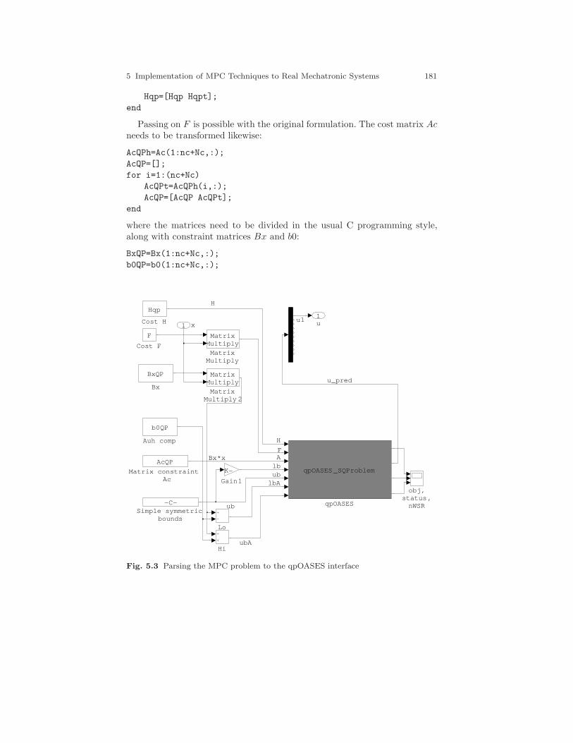
5 Implementation of MPC Techniques to Real Mechatronic Systems 181
Hqp=[Hqp Hqpt];
end
Passing on F is possible with the original formulation. The cost matrix Acneeds to be transformed likewise:
AcQPh=Ac(1:nc+Nc,:);
AcQP=[];
for i=1:(nc+Nc)
AcQPt=AcQPh(i,:);
AcQP=[AcQP AcQPt];
end
where the matrices need to be divided in the usual C programming style,along with constraint matrices Bx and b0:
BxQP=Bx(1:nc+Nc,:);
b0QP=b0(1:nc+Nc,:);
F
H
FF
u1
qpOASES
qpOASES _SQProblem
obj,status ,
nWSRSimple symmetric
bounds
−C−
Matrix constraint Ac
AcQP
MatrixMultiply 2
MatrixMultiply
MatrixMultiply
MatrixMultiply
Lo
Hi
Gain1
−K−
Cost H
Hqp
Cost F
F
Bx
BxQP
Auh comp
b0QP
x1
H
A
u_pred
lb
ub
ublbA
Bx*x
ubA
u1
Fig. 5.3 Parsing the MPC problem to the qpOASES interface
182 Gergely Takacs et al
5.2.3.5 Off-line Simulation
In case an off-line simulation is necessary for results verification or otherpurposes, we may use the Matlab default quadratic solver, named quadprog.To do this, one needs to launch a cycle with one iteration for each samplinginstant and supply the optimization problem to the solver in the followingfashion:
for k=1:run;
[U1(:,k),f,status1(1,k),output]=quadprog(H,F*(X1(:,k)),Ac,b0+
Bx*X1(:,k),[],[],[],[],[],options);
X1(:,k+1)=A*X1(:,k)+B*(U1(1,k))’;
Y1(k)=C*X1(:,k);
end
where X1 is the matrix containing the states and Y 1 is the vector containingthe deflection data. The last two lines assume that there is no need for stateobservation, this is to make the simulation simpler.
If the cost is needed as well, one needs to include either one of the followinglines in the code:
J(k,:)= U1(:,k)’*H*U1(:,k)+2*(X1(:,k))’*F’*U1(:,k)+X1(:,k)’*G
*X1(:,k);
J2(k,:)= X1(:,k)’*Q*X1(:,k)+U1(1,k)’*R*U1(1,k);
The optimization procedure can be fine-tuned by:
options = optimset(’LargeScale’,’off’,’Display’,’off’,’TolFun’
,1e-12);
It is also possible to substitute the Matlab built-in quadprog function withthe qpOASES Matlab interface. After compilation the sequential qpOASESsolver can be simply called by using the following code:
for k=1:run;
[objOA,U2(:,k),yd,status2(1,k),nWSRout2(1,k)]=
qpOASES_sequence(’i’,H,F*X2(:,k),Ac,’’,’’,’’,b0+Bx*X2(:,
k),10);
X2(:,k+1)=A*X2(:,k)+B*U2(1,k);
Y2(k)=C*X2(:,k);
end
5.2.3.6 Controller Loop in Simulink
The QPMPC controller loop is featured in Fig. 5.3. The controller loop con-tains means for A/D and D/A conversion, state observation, data loggingand others. The block containing the QPMPC controller takes the actual ob-server state as an input, and outputs controller voltage. It may be required to
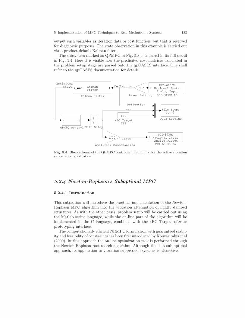
5 Implementation of MPC Techniques to Real Mechatronic Systems 183
output such variables as iteration data or cost function, but that is reservedfor diagnostic purposes. The state observation in this example is carried outvia a product-default Kalman filter.
The subsystem marked as QPMPC in Fig. 5.3 is featured in its full detailin Fig. 5.4. Here it is visible how the predicited cost matrices calculated inthe problem setup stage are parsed onto the qpOASES interface. One shallrefer to the qpOASES documentation for details.
Input
xPC Target TET
TET
Unit Delay
z1
QPMPC control
x u
PCI−6030E DA
PCI−6030ENational Instr.Analog Output
1
PCI−6030E AD
PCI−6030ENational Instr.
Analog Input1
Laser Setting
1.5
Kalman Filter
KalmanFilter ZZZX_estX_estX_estX_estX_estX_est
Data Logging
File ScopeId: 2
Amplifier Compensation
1/20
Estimatedstate
Deflection
Deflection
Input
Fig. 5.4 Block scheme of the QPMPC controller in Simulink, for the active vibrationcancellation application
5.2.4 Newton-Raphson’s Suboptimal MPC
5.2.4.1 Introduction
This subsection will introduce the practical implementation of the Newton-Raphson MPC algorithm into the vibration attenuation of lightly dampedstructures. As with the other cases, problem setup will be carried out usingthe Matlab script language, while the on-line part of the algorithm will beimplemented in the C language, combined with the xPC Target softwareprototyping interface.
The computationally efficient NRMPC formulation with guaranteed stabil-ity and feasibility of constraints has been first introduced by Kouvaritakis et al(2000). In this approach the on-line optimization task is performed throughthe Newton-Raphson root search algorithm. Although this is a sub-optimalapproach, its application to vibration suppression systems is attractive.
184 Gergely Takacs et al
Optimality levels may be enhanced by extending NRMPC by a simpleexplicit additional optimization, as introduced by Kouvaritakis et al (2002).The further development of NRMPC introduced by Cannon and Kouvari-takis (2005) proves to be essential for systems with a significant asymmetryin actuator capabilities and deformation range . The optimization of predic-tion dynamics formulated by Cannon and Kouvaritakis (2005) recovers themaximal possible ellipsoidal region of attraction.
The algorithm described by Kouvaritakis et al (2000), Kouvaritakis et al(2002) and Cannon and Kouvaritakis (2005) serves as a basis for the practi-cal implementation applied to the active vibrating system. For more detailson the theory behind the NRMPC approach, the reader shall refer to theaforementioned publications.
Let us begin with initializing the off-line part of the NRMPC code:
5.2.4.2 Initialization of the Off-line Code
The controller structure is obtained by evaluating linear matrix inequalities(LMI) defined by the invariance and feasibility conditions. LMI are parsedusing YALMIP introduced by L ofberg (2004) to the SeDuMi optimizationsoftware suite as formulated by Sturm (1999).
The first portion of the off-line code initializes the algorithm. Amongstothers, simulation stop time is defined along with the desired deflection, whichin the case of the vibration attenuation example is always zero. A linear time-invariant state space model is loaded from a file. Sampling time is also definedas Ts:
Tstop=60;
yd=0;
load m2ss.mat;
A=m2ss.A; B=m2ss.B; C=m2ss.C; D=m2ss.D;
Ts=0.01;
Other types of settings and tuning parameters are also declared at thebeginning of the script file. Symmetric input constraints are stated as uh.State penalties are set as Q = CTC which includes the output deflection inthe computed cost. Input weighting is declared as the variable R:
uh=120;
Q=C’*C;
R=1e-4;
Prediction cost performance bound γ is stated, which is necessary to belimited in order to preserve numerical stability of the process. A tolerancelimit is also set, which is used to modify the behavior of YALMIP regardingthe handling of strict inequalities.
tolerance=1e-8;
5 Implementation of MPC Techniques to Real Mechatronic Systems 185
gamma=1e6;
Dimensionality of the problem is determined, to allow the use of differentstate-space models for generating predictions:
dim=size(An); dim=dim(1,1);
[w.dim]=size(B); w.dim(1,3)=w.dim(1,1);
w.dim(1,4)=w.dim(1,2)*w.dim(1,3);
w.dim(1,5)=size(Q,1);
Matrix square-roots of the penalization variables are computed. These arerequired in the construction of the invariance condition. The closed loop linearquadratic gain is calculated as well, and it makes use of the prediction modeland penalties introduced earlier:
sqrtR = sqrtm(R); sqrtQ = sqrtm(Q);
K=-dlqr(An,B,Q,sqrtR*sqrtR);
Phi0=(An+B*K);
5.2.4.3 Off-line Variables and Constraints
Four optimization variables are declared, according to the dimensionality ofthe problem. Matrix N is fully parametrized and square, while the rest of theoptimization variables are real valued and symmetric:
Xq = sdpvar(w.dim(1,1),w.dim(1,1));
Yq = sdpvar(w.dim(1,1),w.dim(1,1));
N = sdpvar(w.dim(1,1),w.dim(1,1),’full’);
M = sdpvar(w.dim(1,2),w.dim(1,1));
The LMI constrain the semi-definite programming problem. The set com-mand instructs the parser YALMIP to construct a constraint in an LMIform:
Inv1 = [Yq,Xq;Xq,Xq];
Inv3 = [Phi0*Yq+B*M Phi0*Xq;N+Phi0*Yq+B*M Phi0*Xq];
if (gamma<1/tolerance)
gInv=gamma*eye(w.dim(1,5)+w.dim(1,2));
zInv=zeros(w.dim(1,5)+w.dim(1,2),2*w.dim(1,1));
Inv2=blkdiag(sqrtQ,sqrtR)*[Yq,Xq; K*Yq+M,K*Xq];
F = set([gInv,zInv,Inv2; zInv’,
Inv1,Inv3; Inv2’,Inv3’,Inv1] > 0);
else
F = set([Inv1 Inv3; Inv3’ Inv1] > 0);
end
The if construct checks whether there is an input constraint defined or not.If yes, the feasibility condition is translated to the proper LMI and added to
186 Gergely Takacs et al
the set of constraints defining the SDP problem. Input constraints are definedby:
if ~isempty(uh)
F = F + set([uh^2 [K*Yq+M K*Xq];
[K*Yq+M K*Xq]’ Inv1] > 0);
end
5.2.4.4 Solver Setup and Off-line Solution Initiation
Options are passed to the LMI parser and also to the solver, in this caseSeDuMi. Strict inequality constraints are relaxed and perturbed by the shiftsetting:
ops = sdpsettings(’verbose’,0);
ops = sdpsettings(ops,’shift’,10*tolerance);
ops = sdpsettings(ops,’solver’,’sedumi’,’sedumi.eps’,0)
Solution of the above defined SDP problem is initiated by the solvesdpYALMIP command. The LMI defining constraints are passed onto the solveras the variable F , options are contained in the ops parameter.
The aim of this optimization problem is to maximize the volume of theellipsoids defining the region of attraction and target set. This can be carriedout by utilizing the fact, that the volume of an ellipsoid is proportional to itsdeterminant:
maxε = −(detP )1/m (5.3)
where P is the optimization parameter in general and m is the dimensionof P . In this case optimization objectives and parameters are Y q and Xq,defining the projection and intersection of the augmented ellipsoid into xspace. It is desirable to maximize the volumes of ellipsoids defined by Y q andXq at the same time, by including them in a block diagonal construct.
Optimization parameters Y q,Xq,N andM are converted into the standarddouble precision matrix format, from the YALMIP optimization variable no-tation:
info = solvesdp(F,-geomean(blkdiag(Yq,Xq)),ops);
Yq = double(Yq); Xq = double(Xq);
N = double(N); M = double(M);
5.2.4.5 Factoring, Storing and Preparing Parameters for theOn-line NRMPC Run
After the optimization variables are available, the parameters used in theon-line NRMPC run have to be factored out and stored:
5 Implementation of MPC Techniques to Real Mechatronic Systems 187
[V,XiU] = lu(eye(w.dim(1,1)) - Yq/Xq);
XiU = XiU’;
Qzi = [inv(Xq),XiU;XiU’,-V\(Yq*XiU)];
Qz = [Yq,V;V’,-(Xq*XiU)\V];
Code segments -V\(Yq*XiU) and -(Xq*XiU)\V actually implement mathe-matical operations −V −1YqXiU and −(XqXiU)−1V .
The full, optimized shift matrices A0 and C0 are calculated according to:
A0 = (Xq*XiU)\(N/V’);
C0 = M/V’;
Q11=inv(Xq)
Q12=XiU;
Q21=XiU’;
Q22=-V\(Yq*XiU);
Kt=[K C0];
where code segment (Xq*XiU)\(N/V’) is equivalent to the operation(XqXiU)−1KV T−1.
A matrix right division is used in the segment M/V’ to implement theoperation M/V T−1. After this respective partitions of Qz are stored in vari-ables for the needs of the on-line NRMPC code. It is true that partitions Q12,Q21 are related in symmetry.
5.2.4.6 Cost Transformation
The following code segment is related to cost transformation, and the result-ing conversion of augmented states. The cost to be minimized in the on-lineNRMPC run has been expressed as JNRMPC = fT f which can be only truein the case the augmented states are transformed to make the cost equivalentwith the original MPC formulation.
Mx = dlyap(Phi0’,Q+K’*R*K);
Mc = dlyap(A0’,C0’*(R+B’*Mx*B)*C0);
In order to minimize an equivalent transformed cost and still having thesame simple function, the augmented states z have to be transformed in theon-line optimization task
[V,D]=eig(Mc);
d=sqrt(max(diag(D),tolerance));
invT=V*diag(1./d)/V;
invTT=blkdiag(eye(w.dim(1,1)),invT);
Select parameters are passed onto the on-line formulation, while some mi-nor practical operations are performed in the final code segment.
Pt=invTT’*Qzi*invTT;
188 Gergely Takacs et al
[R,S]=eig(Pt(dim+1:2*dim,dim+1:2*dim));
Sm=diag(S);
Q21=Pt(dim+1:2*dim,1:dim);
5.2.4.7 The Newton-Raphson Root Search Algorithm
The first problem in the on-line formulation is to find λ. For this, one needs touse the Newton-Raphson procedure. The underlying concept is very simple(Anstee, 2006) and in relation to the NRMPC procedure it can be stated as:
dΦ(λ)
dλ=
0− Φ(λ)
λn−1 − λn(5.4)
The procedure itself is also trivial and is represented by the following algo-rithm:
At each sampling instant initialize with λ = 0 and perform an iterationwhich calculates:
λn+1 = λn − Φ(λ)dΦ(λ)dλ
(5.5)
until the change in λ is smaller than the pre-determined tolerance, wheresubscript n denotes the iterations of the Newton-Raphson procedure.
One may take advantage of expressing the matrix Qf as the an eigenval-ue/eigenvector decomposition::
Qif = RΛiRT (5.6)
where R,Λ is defined by the eigenvalue - eigenvector decomposition of Qf andi is the i-th power or inverse. Using the decomposition (5.6) we may denoteM as:
M = Rdiag(1./(1− λSv))RT (5.7)
where “diag” denotes a diagonalization operation, Sv is a vector of eigen-values gained from Λ and ./ denotes the piecewise division operation. Thissubstitutes the inversion of the full matrix expression (I − λQf ) in the on-line algorithm. This expression occurs not only in evaluating the perturbationvector f , but also in the function Φ(λ) and its first derivative.
Let mv = (1 − λSv) and mi = diag(1./m(−i)v ), then:
Φ(λ) = xTkW1m
2W2xk +W3 (5.8)
dΦ(λ)
dλ= 2xT
kW4m3W2xk (5.9)
5 Implementation of MPC Techniques to Real Mechatronic Systems 189
The equation yielding the perturbation vector f will successively transformto
f = λRm1W4xk (5.10)
Matrices W1, W2, W3 can be calculated offline, therefore saving some timeavoiding unnecessary multiplications at every NR iteration and sample time.Matrix W4 can be calculated before the NR process for the actual sampletime initiates:
W1 = QxfR
W2 = WT1
W3 = W1Λ−1
W4 = −xTkW3W2 + xT
k Qxxk − 1
5.2.4.8 Real-time Code Implementation to C
The on-line part of the NRMPC controller is simple. The algorithm does notcontain full matrix inversions, only essential piecewise inversions. Matrix andvector operations within the NRMPC on-line algorithm are performed usingthe Basic Linear Algebra Subprograms (BLAS) package.
The Simulink scheme implementing the NRMPC controller gains its feed-back signal directly from a block reading the analogue input of the measure-ment card. The scheme is visible in Fig. 5.5. The output from this block isscaled according to the current settings of the LASER head, so its outputis given directly in millimetres. The File Scope block ensures real-time datalogging onto the xPC Target PC hard drive, which can be later re-used formeasurement processing.
Feedback measurement passes through a product default Kalman filter,a part of the Signal Processing Blockset toolbox (MathWorks, 2007). TheKalman filter is always enabled, and the number of filters is set to one. Initialcondition is assumed to be zero.
The estimated state, conforming to the dimensions of model consideredwhen creating the NRMPC controller, is passed onto a custom S-Functionblock implementing the on-line NRMPC code in C language. This block takesparameters R, T, Sm, Q21, Q11,K and C0 as its set-up and starting param-eters. All of these parameters are the result of running the Matlab scriptresponsible for initialization and off-line NRMPC algorithm evaluation. TheS-Function block has the core C program and two custom functions (See5.2.4.9) specified as modules.
The C program is contained within this S-Function, which has been createdusing the S-Function Builder. In addition to the specified parameters includ-ing their data type, input and output ports are declared. Here the input is theestimated state, and output the scalar controller variable. Discrete sampling
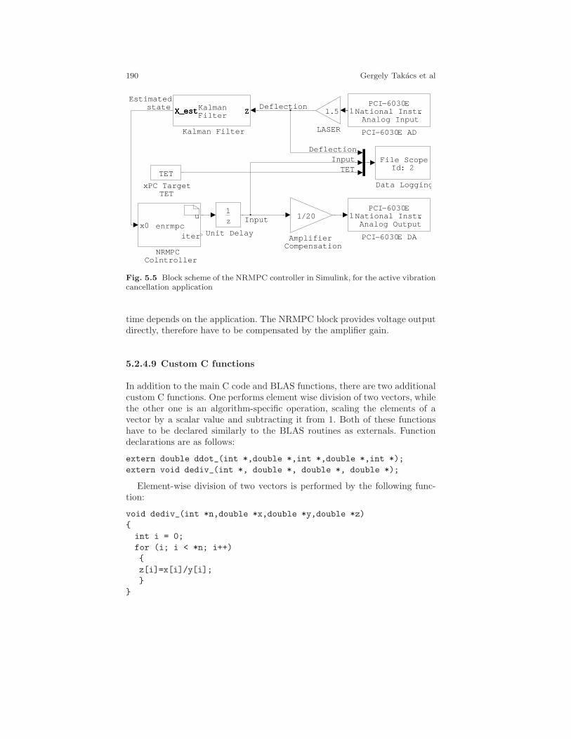
190 Gergely Takacs et al
xPC Target TET
TET
Unit Delay
z1
PCI−6030E DA
PCI−6030ENational Instr.Analog Output
1
PCI−6030E AD
PCI−6030ENational Instr.
Analog Input1
NRMPC Colntroller
enrmpcx0u
iter
LASER
1.5
Kalman Filter
KalmanFilter ZZZX_estX_estX_estX_estX_estX_est
Data Logging
File ScopeId: 2
Amplifier Compensation
1/20
Estimatedstate
Deflection
Deflection
TETInput
Input
Fig. 5.5 Block scheme of the NRMPC controller in Simulink, for the active vibrationcancellation application
time depends on the application. The NRMPC block provides voltage outputdirectly, therefore have to be compensated by the amplifier gain.
5.2.4.9 Custom C functions
In addition to the main C code and BLAS functions, there are two additionalcustom C functions. One performs element wise division of two vectors, whilethe other one is an algorithm-specific operation, scaling the elements of avector by a scalar value and subtracting it from 1. Both of these functionshave to be declared similarly to the BLAS routines as externals. Functiondeclarations are as follows:
extern double ddot_(int *,double *,int *,double *,int *);
extern void dediv_(int *, double *, double *, double *);
Element-wise division of two vectors is performed by the following func-tion:
void dediv_(int *n,double *x,double *y,double *z)
int i = 0;
for (i; i < *n; i++)
z[i]=x[i]/y[i];
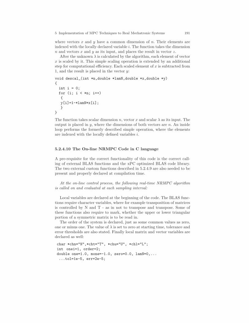
5 Implementation of MPC Techniques to Real Mechatronic Systems 191
where vectors x and y have a common dimension of n. Their elements areindexed with the locally declared variable i. The function takes the dimensionn and vectors x and y as its input, and places the result in vector z.
After the unknown λ is calculated by the algorithm, each element of vectorx is scaled by it. This simple scaling operation is extended by an additionalstep for computational efficiency. Each scaled element of x is subtracted from1, and the result is placed in the vector y:
void descal_(int *n,double *lamN,double *x,double *y)
int i = 0;
for (i; i < *n; i++)
y[i]=1-*lamN*x[i];
The function takes scalar dimension n, vector x and scalar λ as its input. Theoutput is placed in y, where the dimensions of both vectors are n. An insideloop performs the formerly described simple operation, where the elementsare indexed with the locally defined variables i.
5.2.4.10 The On-line NRMPC Code in C language
A pre-requisite for the correct functionality of this code is the correct call-ing of external BLAS functions and the xPC optimized BLAS code library.The two external custom functions described in 5.2.4.9 are also needed to bepresent and properly declared at compilation time.
At the on-line control process, the following real-time NRMPC algorithmis called on and evaluated at each sampling interval:
Local variables are declared at the beginning of the code. The BLAS func-tions require character variables, where for example transposition of matricesis controlled by N and T - as in not to transpose and transpose. Some ofthese functions also require to mark, whether the upper or lower triangularportion of a symmetric matrix is to be read in.
The order of the system is declared, just as some common values as zero,one or minus one. The value of λ is set to zero at starting time, tolerance anderror thresholds are also stated. Finally local matrix and vector variables aredeclared as well:
char *chn="N",*cht="T", *chu="U", *chl="L";
int onei=1, order=2;
double one=1.0, mone=-1.0, zero=0.0, lamN=0,...
...tol=1e-5, err=2e-5;
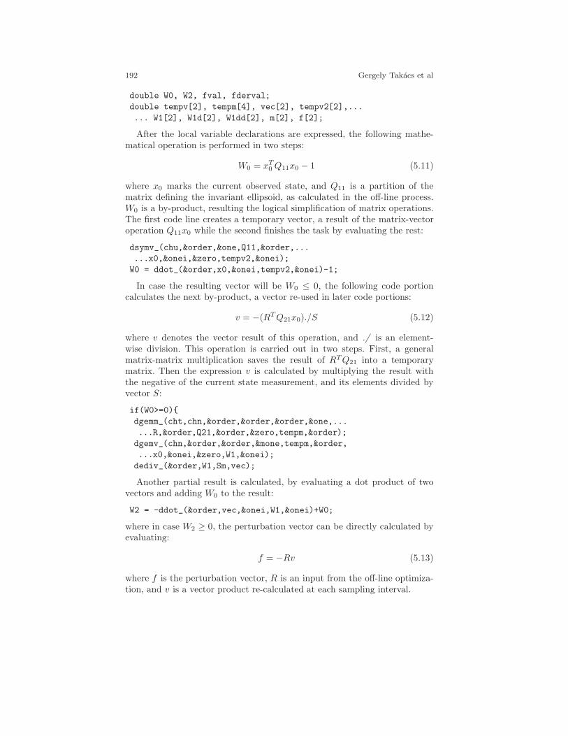
192 Gergely Takacs et al
double W0, W2, fval, fderval;
double tempv[2], tempm[4], vec[2], tempv2[2],...
... W1[2], W1d[2], W1dd[2], m[2], f[2];
After the local variable declarations are expressed, the following mathe-matical operation is performed in two steps:
W0 = xT0 Q11x0 − 1 (5.11)
where x0 marks the current observed state, and Q11 is a partition of thematrix defining the invariant ellipsoid, as calculated in the off-line process.W0 is a by-product, resulting the logical simplification of matrix operations.The first code line creates a temporary vector, a result of the matrix-vectoroperation Q11x0 while the second finishes the task by evaluating the rest:
dsymv_(chu,&order,&one,Q11,&order,...
...x0,&onei,&zero,tempv2,&onei);
W0 = ddot_(&order,x0,&onei,tempv2,&onei)-1;
In case the resulting vector will be W0 ≤ 0, the following code portioncalculates the next by-product, a vector re-used in later code portions:
v = −(RTQ21x0)./S (5.12)
where v denotes the vector result of this operation, and ./ is an element-wise division. This operation is carried out in two steps. First, a generalmatrix-matrix multiplication saves the result of RTQ21 into a temporarymatrix. Then the expression v is calculated by multiplying the result withthe negative of the current state measurement, and its elements divided byvector S:
if(W0>=0)
dgemm_(cht,chn,&order,&order,&order,&one,...
...R,&order,Q21,&order,&zero,tempm,&order);
dgemv_(chn,&order,&order,&mone,tempm,&order,
...x0,&onei,&zero,W1,&onei);
dediv_(&order,W1,Sm,vec);
Another partial result is calculated, by evaluating a dot product of twovectors and adding W0 to the result:
W2 = -ddot_(&order,vec,&onei,W1,&onei)+W0;
where in case W2 ≥ 0, the perturbation vector can be directly calculated byevaluating:
f = −Rv (5.13)
where f is the perturbation vector, R is an input from the off-line optimiza-tion, and v is a vector product re-calculated at each sampling interval.
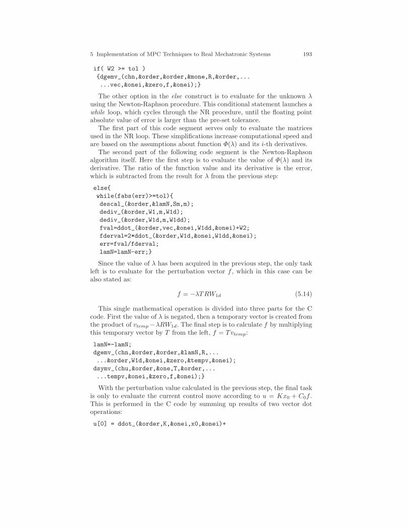
5 Implementation of MPC Techniques to Real Mechatronic Systems 193
if( W2 >= tol )
dgemv_(chn,&order,&order,&mone,R,&order,...
...vec,&onei,&zero,f,&onei);
The other option in the else construct is to evaluate for the unknown λusing the Newton-Raphson procedure. This conditional statement launches awhile loop, which cycles through the NR procedure, until the floating pointabsolute value of error is larger than the pre-set tolerance.
The first part of this code segment serves only to evaluate the matricesused in the NR loop. These simplifications increase computational speed andare based on the assumptions about function Φ(λ) and its i-th derivatives.
The second part of the following code segment is the Newton-Raphsonalgorithm itself. Here the first step is to evaluate the value of Φ(λ) and itsderivative. The ratio of the function value and its derivative is the error,which is subtracted from the result for λ from the previous step:
else
while(fabs(err)>=tol)
descal_(&order,&lamN,Sm,m);
dediv_(&order,W1,m,W1d);
dediv_(&order,W1d,m,W1dd);
fval=ddot_(&order,vec,&onei,W1dd,&onei)+W2;
fderval=2*ddot_(&order,W1d,&onei,W1dd,&onei);
err=fval/fderval;
lamN=lamN-err;
Since the value of λ has been acquired in the previous step, the only taskleft is to evaluate for the perturbation vector f , which in this case can bealso stated as:
f = −λTRW1d (5.14)
This single mathematical operation is divided into three parts for the Ccode. First the value of λ is negated, then a temporary vector is created fromthe product of vtemp−λRW1d. The final step is to calculate f by multiplyingthis temporary vector by T from the left, f = Tvtemp:
lamN=-lamN;
dgemv_(chn,&order,&order,&lamN,R,...
...&order,W1d,&onei,&zero,&tempv,&onei);
dsymv_(chu,&order,&one,T,&order,...
...tempv,&onei,&zero,f,&onei);
With the perturbation value calculated in the previous step, the final taskis only to evaluate the current control move according to u = Kx0 + C0f .This is performed in the C code by summing up results of two vector dotoperations:
u[0] = ddot_(&order,K,&onei,x0,&onei)+
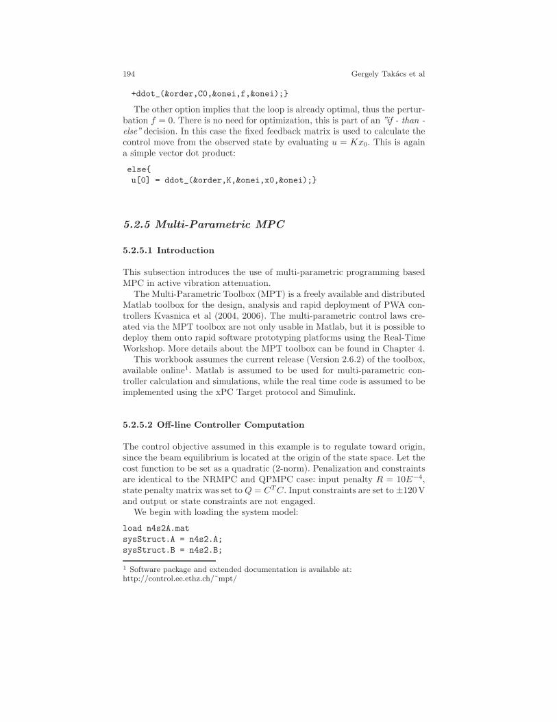
194 Gergely Takacs et al
+ddot_(&order,C0,&onei,f,&onei);
The other option implies that the loop is already optimal, thus the pertur-bation f = 0. There is no need for optimization, this is part of an ”if - than -else” decision. In this case the fixed feedback matrix is used to calculate thecontrol move from the observed state by evaluating u = Kx0. This is againa simple vector dot product:
else
u[0] = ddot_(&order,K,&onei,x0,&onei);
5.2.5 Multi-Parametric MPC
5.2.5.1 Introduction
This subsection introduces the use of multi-parametric programming basedMPC in active vibration attenuation.
The Multi-Parametric Toolbox (MPT) is a freely available and distributedMatlab toolbox for the design, analysis and rapid deployment of PWA con-trollers Kvasnica et al (2004, 2006). The multi-parametric control laws cre-ated via the MPT toolbox are not only usable in Matlab, but it is possible todeploy them onto rapid software prototyping platforms using the Real-TimeWorkshop. More details about the MPT toolbox can be found in Chapter 4.
This workbook assumes the current release (Version 2.6.2) of the toolbox,available online1. Matlab is assumed to be used for multi-parametric con-troller calculation and simulations, while the real time code is assumed to beimplemented using the xPC Target protocol and Simulink.
5.2.5.2 Off-line Controller Computation
The control objective assumed in this example is to regulate toward origin,since the beam equilibrium is located at the origin of the state space. Let thecost function to be set as a quadratic (2-norm). Penalization and constraintsare identical to the NRMPC and QPMPC case: input penalty R = 10E−4,state penalty matrix was set to Q = CTC. Input constraints are set to ±120Vand output or state constraints are not engaged.
We begin with loading the system model:
load n4s2A.mat
sysStruct.A = n4s2.A;
sysStruct.B = n4s2.B;
1 Software package and extended documentation is available at:http://control.ee.ethz.ch/˜mpt/
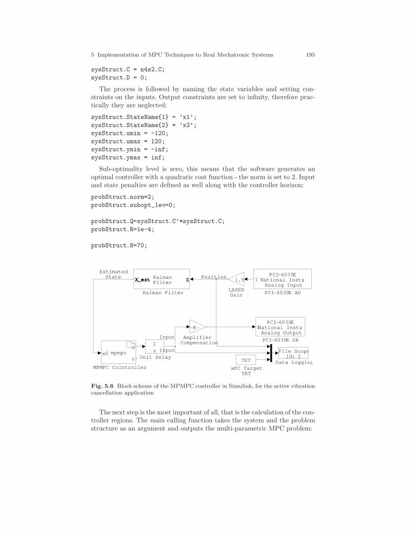
5 Implementation of MPC Techniques to Real Mechatronic Systems 195
sysStruct.C = n4s2.C;
sysStruct.D = 0;
The process is followed by naming the state variables and setting con-straints on the inputs. Output constraints are set to infinity, therefore prac-tically they are neglected:
sysStruct.StateName1 = ’x1’;
sysStruct.StateName2 = ’x2’;
sysStruct.umin = -120;
sysStruct.umax = 120;
sysStruct.ymin = -inf;
sysStruct.ymax = inf;
Sub-optimality level is zero, this means that the software generates anoptimal controller with a quadratic cost function - the norm is set to 2. Inputand state penalties are defined as well along with the controller horizon:
probStruct.norm=2;
probStruct.subopt_lev=0;
probStruct.Q=sysStruct.C’*sysStruct.C;
probStruct.R=1e-4;
probStruct.N=70;
xPC Target TET
TETUnit Delay
z
1PCI−6030E DA
PCI−6030ENational Instr.Analog Output
1
PCI−6030E AD
PCI−6030ENational Instr.
Analog Input1
MPMPC Colntroller
mpmpcx0u
r
LASERGain
1.5
Kalman Filter
KalmanFilter ZZZX_estX_estX_estX_estX_estX_est
Data Logging
File ScopeId: 2
Amplifier Compensation
−K−
EstimatedState Position
Input
Input
Fig. 5.6 Block scheme of the MPMPC controller in Simulink, for the active vibrationcancellation application
The next step is the most important of all, that is the calculation of the con-troller regions. The main calling function takes the system and the problemstructure as an argument and outputs the multi-parametric MPC problem:
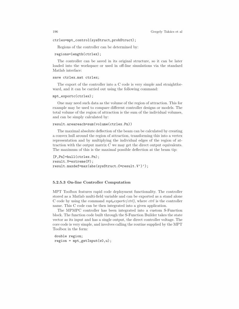
196 Gergely Takacs et al
ctrlex=mpt_control(sysStruct,probStruct);
Regions of the controller can be determined by:
regions=length(ctrlex);
The controller can be saved in its original structure, so it can be laterloaded into the workspace or used in off-line simulations via the standardMatlab interface:
save ctrlex.mat ctrlex;
The export of the controller into a C code is very simple and straightfor-ward, and it can be carried out using the following command:
mpt_exportc(ctrlex);
One may need such data as the volume of the region of attraction. This forexample may be used to compare different controller designs or models. Thetotal volume of the region of attraction is the sum of the individual volumes,and can be simply calculated by:
result.areareach=sum(volume(ctrlex.Pn))
The maximal absolute deflection of the beam can be calculated by creatinga convex hull around the region of attraction, transforming this into a vertexrepresentation and by multiplying the individual edges of the region of at-traction with the output matrix C we may get the direct output equivalents.The maximum of this is the maximal possible deflection at the beam tip:
[P,Pn]=hull(ctrlex.Pn);
result.V=extreme(P);
result.maxdef=max(abs(sysStruct.C*result.V’)’);
5.2.5.3 On-line Controller Computation
MPT Toolbox features rapid code deployment functionality. The controllerstored as a Matlab multi-field variable and can be exported as a stand aloneC code by using the command mpt exportc(ctrl), where ctrl is the controllername. This C code can be then integrated into a given application.
The MPMPC controller has been integrated into a custom S-Functionblock. The function code built through the S-Function Builder takes the statevector as its input and has a single output, the direct controller voltage. Thecore code is very simple, and involves calling the routine supplied by the MPTToolbox in the form:
double region;
region = mpt_getInput(x0,u);
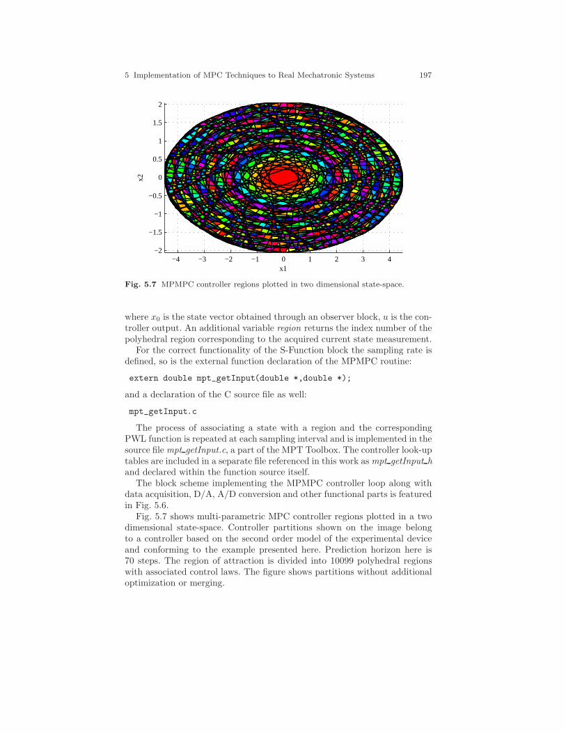
5 Implementation of MPC Techniques to Real Mechatronic Systems 197
−4 −3 −2 −1 0 1 2 3 4−2
−1.5
−1
−0.5
0
0.5
1
1.5
2
x1
x2
Fig. 5.7 MPMPC controller regions plotted in two dimensional state-space.
where x0 is the state vector obtained through an observer block, u is the con-troller output. An additional variable region returns the index number of thepolyhedral region corresponding to the acquired current state measurement.
For the correct functionality of the S-Function block the sampling rate isdefined, so is the external function declaration of the MPMPC routine:
extern double mpt_getInput(double *,double *);
and a declaration of the C source file as well:
mpt_getInput.c
The process of associating a state with a region and the correspondingPWL function is repeated at each sampling interval and is implemented in thesource file mpt getInput.c, a part of the MPT Toolbox. The controller look-uptables are included in a separate file referenced in this work asmpt getInput hand declared within the function source itself.
The block scheme implementing the MPMPC controller loop along withdata acquisition, D/A, A/D conversion and other functional parts is featuredin Fig. 5.6.
Fig. 5.7 shows multi-parametric MPC controller regions plotted in a twodimensional state-space. Controller partitions shown on the image belongto a controller based on the second order model of the experimental deviceand conforming to the example presented here. Prediction horizon here is70 steps. The region of attraction is divided into 10099 polyhedral regionswith associated control laws. The figure shows partitions without additionaloptimization or merging.
198 Gergely Takacs et al
−4−2
02
4
−2−1
01
2−40
−20
0
20
40
x1
x2
U* 1(x
)
Fig. 5.8 MPMPC controller input in volts.
MPMPC controller action expressed in Volts is plotted against the statespace in two dimensions in Fig. 5.8. Note how the control law is essentiallyreduced to a switching behaviour. In fact many real and simple vibrationcontrol systems utilize this highly simplified saturated effect.
Fig. 5.9 shows the plot of the quadratic cost function value J∗, related tothe polytopic controller regions in state-space.
5.2.6 Conclusion
This section has been dealing with the implementation of model predictivecontrol algorithms in the engineering field of active vibration attenuation. Dueto the nature of the problem very short sampling times are required, moreoverlarge actuator asymmetry can render the MPC problem quite formidable.
If the control process is augmented with guaranteed stability and feasibilityrequirements, the useful states are limited inside a portion of the otherwiseinfinitely large state-space. This portion of the state-space is called the regionof attraction. If the expected deformations of under-damped systems belongto a wide scale region, we have to ensure a matching region of attraction.
A good example of such and similar vibrational systems are for examplehelicopter rotor beams or solar panels in a microgravity environment. Thischapter introduced a simple laboratory system, which emulated the physicalproperties and dynamic behaviour of the aforementioned class of engineering
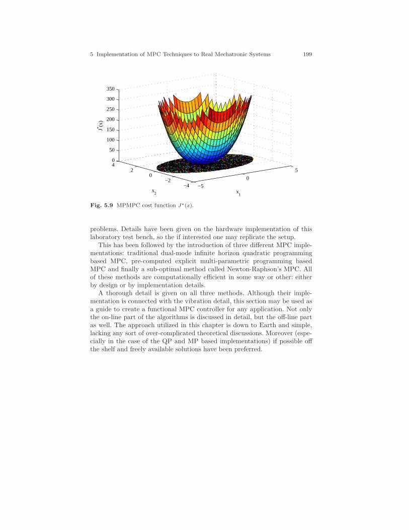
5 Implementation of MPC Techniques to Real Mechatronic Systems 199
−5
0
5
−4−2
02
40
50
100
150
200
250
300
350
x1
x2
J* (x)
Fig. 5.9 MPMPC cost function J∗(x).
problems. Details have been given on the hardware implementation of thislaboratory test bench, so the if interested one may replicate the setup.
This has been followed by the introduction of three different MPC imple-mentations: traditional dual-mode infinite horizon quadratic programmingbased MPC, pre-computed explicit multi-parametric programming basedMPC and finally a sub-optimal method called Newton-Raphson’s MPC. Allof these methods are computationally efficient in some way or other: eitherby design or by implementation details.
A thorough detail is given on all three methods. Although their imple-mentation is connected with the vibration detail, this section may be used asa guide to create a functional MPC controller for any application. Not onlythe on-line part of the algorithms is discussed in detail, but the off-line partas well. The approach utilized in this chapter is down to Earth and simple,lacking any sort of over-complicated theoretical discussions. Moreover (espe-cially in the case of the QP and MP based implementations) if possible offthe shelf and freely available solutions have been preferred.
200 Gergely Takacs et al
5.3 Implementation of Predictive Control of Air-FuelRatio in Spark Ignition Engine
5.3.1 Introduction
A run of a spark ignition engine (SI) is highly dependent on the mixture ofthe sucked air and injected fuel present in the cylinder, waiting to be ignitedby the spark. Incorrect ratio of this two components may lead to the poorengine power, ineffective functionality of the catalytic converter resulting inhigher level of emissions polluting the environment and in the extreme casethis can lead to the engine stoppage. Due to this reason it is crucial to keepthe air/fuel ratio (AFR) at the stoichiometric level, which means, that both,the air and the fuel are completely combusted. Due to above mentioned rea-sons and all the time tightening emission standards the car producers areimproving the control of the air/fuel ratio.Traditional control of air/fuel ratio is based on a feedforward control usingpredefined tables determining how much fuel has to be injected into a cylin-der, based on the information from the mass air flow meter. This fuel amountis subsequently corrected using the information from the lambda probe, sothe stoichiometric mixture can be reached. Due to a lambda probe position(at the engine exhaust) a delay arises, causing an improper feedback cor-rection at the unstable engine regimes, like acceleration, or deceleration. Onthe other side, this kind of control guarantees stability and robustness at allconditions and therefore is still preferred by car producers, despite its disad-vantages in control.The academic field have started to publish other kinds of air/fuel control,mostly model-based ones. The model-based approaches are bringing goodquality of control, but are also more sensitive to the model precision and is-sues with stability and robustness appear. A survey through popular ”meanvalue engine modeling” is described in Bengtsson et al (2007). This analyticalway of engine modeling is very clear, but requires exact knowledge of the sys-tem and the model error has to be taken into account explicitly. Other waysof a model acquisition are based on the experimental identification (black boxmodeling). Works of Zhai et al (2010), Zhai and Yu (2009) and Hou (2007)are specialized in employment of neural networks, while Mao et al (2009) usesfor engine modeling CARIMA models.In the engine control itself became popular fuzzy logic (Hou (2007)), neuralnetwork control (Arsie et al (2008)) and model predictive control (MPC) ap-proaches (Lorini et al (2006) and Muske and Jones (2006)). General topicson an issue of stability and robustness in MPC can be found in Mayne et al(2000b), or Zeman and Rohal-Ilkiv (2003).Our approach, introduced in Poloni et al (2007) is utilizing an analyticalmodel predictive controller with a penalization of a terminal state. It usesa multi-model approach using a weighted net (sugeno-type fuzzy logic) of
5 Implementation of MPC Techniques to Real Mechatronic Systems 201
autoregressive models (ARX) as a system model. The ARX models wereidentified in the particular working points of the engine as black box mod-els. This method of engine modeling offers an easy way of ”global nonlinearsystem model”acquisition with subsequent utilization in the model based sys-tem control. The preliminary real-time predictive control results presented inthis paper indicate that the proposed controller could be suitable alternativetoward the air/fuel ratio control through the look-up tables.
5.3.2 Hardware Description
The engine test bench consists of several components, building up together aflexible and freely programmable system, perfectly suitable for engine controland research.One part of the test bench is a combustion engine itself, rigidly connected tothe eddy current brake. As an interface and a communication part is utilizeda rapid control prototyping system based on dSpace hardware. This allows toexecute the designed controllers of the air/fuel ratio on the engine, insteadof the original electronic control unit (ECU).
5.3.2.1 Combustion Engine
For the experiments and measurements has been used a spark ignition enginefrom the Volkswagen Polo 1.4 16V (Fig. 5.10). It is a four-cylinder in-lineengine with a DOHC valve train.
Engine characteristics:
• Engine code: AUA• Volume: 1390ccm• Number of cylinders: 4• Number of valves: 16• Bore x stroke: 76.5 x 75.6mm• Compression ratio: 10.5• Power: 55kW (75k) at 5000 rpm• Torque: 126Nm at 3800 rpm• Injection system: multipoint, sequential, 1 injector per valve• Ignition: electronic, independent injectors• Fuel: Natural 95• Emissions processing: three way catalys
The original Bosch ECU has been completely replaced by a rapid proto-typing system. It is dedicated for the control of power stages, as injectors andignitors, as described in the Subsection 5.3.2.3.
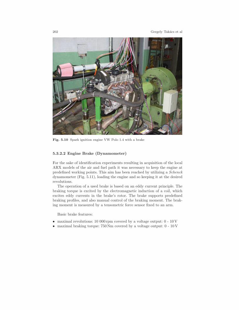
202 Gergely Takacs et al
Fig. 5.10 Spark ignition engine VW Polo 1.4 with a brake
5.3.2.2 Engine Brake (Dynamometer)
For the sake of identification experiments resulting in acquisition of the localARX models of the air and fuel path it was necessary to keep the engine atpredefined working points. This aim has been reached by utilizing a Schenckdynamometer (Fig. 5.11), loading the engine and so keeping it at the desiredrevolutions.
The operation of a used brake is based on an eddy current principle. Thebraking torque is excited by the electromagnetic induction of a coil, whichexcites eddy currents in the brake’s rotor. The brake supports predefinedbraking profiles, and also manual control of the braking moment. The brak-ing moment is measured by a tensometric force sensor fixed to an arm.
Basic brake features:
• maximal revolutions: 10 000 rpm covered by a voltage output: 0 - 10V• maximal braking torque: 750Nm covered by a voltage output: 0 - 10V

5 Implementation of MPC Techniques to Real Mechatronic Systems 203
The control unit of a brake is an independent device allowing the manualbrake control by analog voltage signals. It includes the following circuits:
• “thyristor phase” control circuit (braking moment)• revolutions measurement circuit• braking moment measurement circuit
The“thyristor phase”control circuit is based on the integrated circuit (IC)TCA785. Function of this IC is a phase control of a brake’s power stage. Thecontrol voltage span is 0 - 10V, corresponding to the braking moment. Thebraking moment is used for the aim of:
• regulation to constant revolutions, based on a discrete PI controller• regulation to a particular braking moment
Fig. 5.11 Engine brake
5.3.2.3 Rapid Control Prototyping System
The computational unit necessary for the real-time implementation of theMPC control is based on a powerful and freely programmable control systembased on dSpace and RapidPro units; or “Rapid Control Prototyping System”(RCP), (Fig. 5.13, dSPACE GmbH. (2009)).It is built up on the processor board ds1005 and hardware-in-loop platform

204 Gergely Takacs et al
dS2202 HIL.
The main components are (Fig. 5.12):
• DS1005 PPC Board - processor module• DS2202 HIL I/O Board - module of input/output interface• DS4121 ECU Interface Board - interface for the communication with the
ECU
DS1005 PPC Board
DS1005 PPC Board is a core processor module of the dSpace system. It hasa huge computational power for the real-time applications and creates aninterface between the input/output circuits and the host computer. DS1005is suitable for the systems with fast dynamics with a high computationalload.Basic features:
• processor PowerPC 750GX, 1 GHz• fully programmable from Simulink environment• fast communication between dSpace modules over PHS bus
Module DS2202 HIL I/O Board
The DS2202 HIL I/O Board module has been designed for the hardware-in-the-loop simulations in automobile industry applications. It supports mea-surements and and control of various peripheral devices typical for differentautomobile systems.Module features:
• 20 D/A channels a 16 A/D channels• 38 digital inputs and 16 digital outputs• supports 12 to 42V voltage systems
Modul DS4121
Module DS4121 is an interface between the ECU or RapidPro unit and thedSpace modular system. It has a support for two independent ECUs. Theflexibility of this solution allows to control the power stages of the engine,gearbox, or the valve train for a up to 12 cylinder engine.
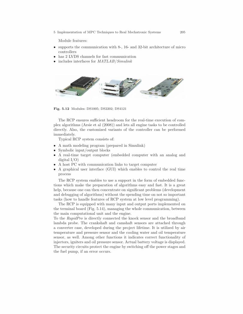
5 Implementation of MPC Techniques to Real Mechatronic Systems 205
Module features:
• supports the communication with 8-, 16- and 32-bit architecture of microcontrollers
• has 2 LVDS channels for fast communication• includes interfaces for MATLAB/Simulink
Fig. 5.12 Modules: DS1005; DS2202; DS4121
The RCP ensures sufficient headroom for the real-time execution of com-plex algorithms (Arsie et al (2008)) and lets all engine tasks to be controlleddirectly. Also, the customized variants of the controller can be performedimmediately.
Typical RCP system consists of:
• A math modeling program (prepared in Simulink)• Symbolic input/output blocks• A real-time target computer (embedded computer with an analog and
digital I/O)• A host PC with communication links to target computer• A graphical user interface (GUI) which enables to control the real time
process
The RCP system enables to use a support in the form of embedded func-tions which make the preparation of algorithms easy and fast. It is a greathelp, because one can then concentrate on significant problems (developmentand debugging of algorithms) without the spending time on not so importanttasks (how to handle features of RCP system at low level programming).
The RCP is equipped with many input and output ports implemented onthe terminal board (Fig. 5.14), managing the whole communication, betweenthe main computational unit and the engine.To the RapidPro is directly connected the knock sensor and the broadbandlambda probe. The crankshaft and camshaft sensors are attached througha converter case, developed during the project lifetime. It is utilized by airtemperature and pressure sensor and the cooling water and oil temperaturesensor, as well. Among other functions it indicates correct functionality ofinjectors, igniters and oil pressure sensor. Actual battery voltage is displayed.The security circuits protect the engine by switching off the power stages andthe fuel pump, if an error occurs.
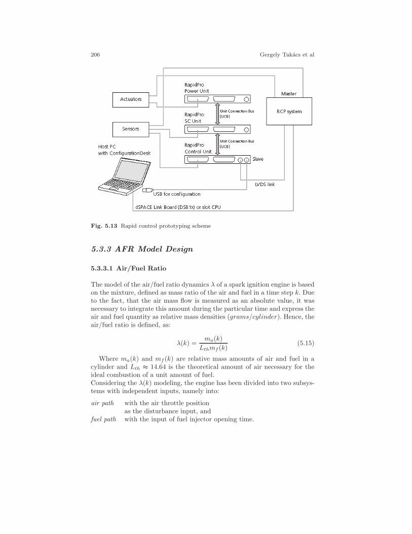
206 Gergely Takacs et al
Fig. 5.13 Rapid control prototyping scheme
5.3.3 AFR Model Design
5.3.3.1 Air/Fuel Ratio
The model of the air/fuel ratio dynamics λ of a spark ignition engine is basedon the mixture, defined as mass ratio of the air and fuel in a time step k. Dueto the fact, that the air mass flow is measured as an absolute value, it wasnecessary to integrate this amount during the particular time and express theair and fuel quantity as relative mass densities (grams/cylinder). Hence, theair/fuel ratio is defined, as:
λ(k) =ma(k)
Lthmf (k)(5.15)
Where ma(k) and mf (k) are relative mass amounts of air and fuel in acylinder and Lth ≈ 14.64 is the theoretical amount of air necessary for theideal combustion of a unit amount of fuel.Considering the λ(k) modeling, the engine has been divided into two subsys-tems with independent inputs, namely into:
air path with the air throttle positionas the disturbance input, and
fuel path with the input of fuel injector opening time.
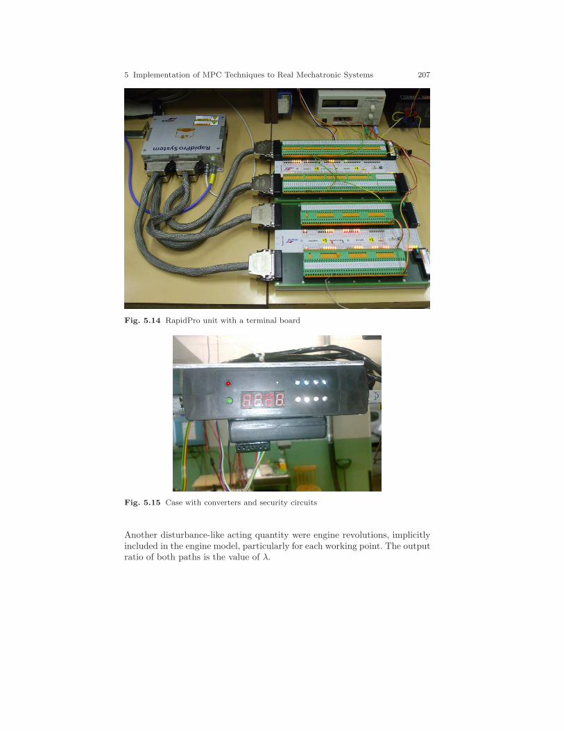
5 Implementation of MPC Techniques to Real Mechatronic Systems 207
Fig. 5.14 RapidPro unit with a terminal board
Fig. 5.15 Case with converters and security circuits
Another disturbance-like acting quantity were engine revolutions, implicitlyincluded in the engine model, particularly for each working point. The outputratio of both paths is the value of λ.
208 Gergely Takacs et al
5.3.3.2 SI Engine Modeling using ARX Models
The engine modeling is based on the weighted linear local model with singleinput single output (SISO) structure (Poloni et al (2008)). The parametersof local linear ARX models with weighted validity (Murray-Smith and Jo-hanssen (1997)) are identified to model AFR nonlinear dynamics. The prin-ciple of this nonlinear modeling technique is in partitioning of the engine’sworking range into smaller working points.
A net of local ARX models weighted for a particular working point φ isdefined, as:
∑nM
h=1 ρh(φ(k))Ah(q)y(k) =∑nM
h=1 ρh(φ(k))Bh(q)u(k) +∑nM
h=1 ρh(φ(k))ch + e(k)(5.16)
defined by polynomials Ah and Bh:
Ah(q) = 1 + ah,1q−1 + . . .+ ah,ny
q−ny
Bh(q) = bh,1+dhq−1−dh + . . .+ bh,nu+dh
q−nu−dh(5.17)
where symbolics q−i denotes a sample delay, e.x. q−iy(k) = y(k − i), ah,iand bh,(j+dh) are parameters of h-th local function and dh is its delay. Pa-rameter nM represents the number of local models.
The ρh denotes a weighting function for a particular ARX model (seeSec. 5.3.3.4) and e(k) is a stochastic term with a white noise properties.The engine working point itself is defined by engine revolutions nen and thethrottle valve position tr, hence: φ(k) = [nen(k), tr(k)]
T . The absolute termch of the equation is computed from the steady state values of the systemoutput ye,h and the system input ue,h, as:
ch = ye,h + ye,h
ny∑
i=1
ah,i − ue,h
nu∑
j=1
bh,j (5.18)
The model output is computed from the equation:
ys(k) =∑nM
h=1 ρh(φ(k))
·(∑ny
i=1 ah,iq−iys(k) +
∑nuj=1 bh,(j+dh)q
−j−dhu(k) + ch
)(5.19)
Introducing the estimated parameter vector θh and the regression vectorγ(k), equation (5.19) becomes:
ys(k) = γT (k)
nM∑
h=1
ρh(φ(k))θh +
nM∑
h=1
ρh(φ(k))ch (5.20)
5 Implementation of MPC Techniques to Real Mechatronic Systems 209
5.3.3.3 Model Identification
Parameters of the local ARX models have been estimated from the dataacquired from the exhaust gas oxygen sensor and an air flow sensor. Theidentification has been designed so, that the dynamics of the air path andfuel path stayed uncoupled. Dynamics of both paths were measured indi-rectly.The first experiment started at the stoichiometric value of λa in the opera-tion point φ. To excite the air path dynamics, the throttle valve position wasoscillating around its steady position according to a pseudo-random binarysignal (PRBS, Fig. 5.16), while the fuel injectors were delivering constant fuelmass mf,e. The change in λa value has been recorded. During the experimentthe engine had been braked at constant revolutions.The PRBS signal is a signal changing its value binary, that means from onelevel to another with a pseudo-randomly changing period (Fig. 16(a)). Thisperiod has to be chosen with respect to the identified system so, that foreven smallest change in PRBS a clear system response can be noticed. Thiscondition has to be ensured, to excite the entire system dynamics and con-sequently to perform a relevant system identification. The Fig. 16(b) showsan example of a correctly identified system with a good fit, compared to theoriginal data (system output).The identification of the fuel path dynamics has been done similarly, but withthe fixed throttle valve delivering a constant air massma,e. The PRBS is vary-ing the fuel injectors’ opening time. In both experiments it was necessary towisely propose a PRBS, so that the air/fuel mixture is always ignitable.The local ARX models can be subsequently determined from the measuredvalues of instantaneous λa(k) and λf (k) belonging to the air path and fuelpath, utilizing relative air and fuel mass densities, as:
ma(k) = ma,e(φ)λa(k) (5.21)
mf (k) =mf,e(φ)
λf (k)(5.22)
The final formula describing the aif/fuel ratio dynamics is built up of locallinear ARX models of the air and fuel paths is in the form:
λs(k) =1
Lth
·[γTa (k)
∑nAh=1
ρa,h(φ(k))θa,h+∑nA
h=1ρa,h(φ(k))ca,h
γTf(k)
∑nFh=1
ρf,h(φ(k))θf,h+∑nF
h=1ρf,h(φ(k))cf,h
](5.23)
Where:
γ is the regression vector of system inputs and outputsnA is the amount of working pointsρ is the interpolation functionφ is the vector of a working point
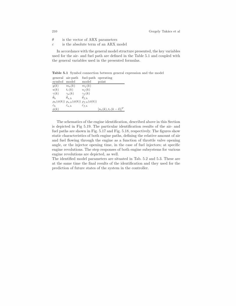
210 Gergely Takacs et al
θ is the vector of ARX parametersc is the absolute term of an ARX model
In accordance with the general model structure presented, the key variablesused for the air- and fuel path are defined in the Table 5.1 and coupled withthe general variables used in the presented formulas.
Table 5.1 Symbol connection between general expression and the model
general air-path fuel-path operatingsymbol model model pointy(k) ma(k) mf (k)u(k) tr(k) uf (k)γ(k) γa(k) γf (k)
θh θa,h θf,hρh(φ(k)) ρa,h(φ(k)) ρf,h(φ(k))ch ca,h cf,hφ(k) [ne(k), tr(k − δ)]T
The schematics of the engine identification, described above in this Sectionis depicted in Fig 5.19. The particular identification results of the air- andfuel paths are shown in Fig. 5.17 and Fig. 5.18, respectively. The figures showstatic characteristics of both engine paths, defining the relative amount of airand fuel flowing through the engine as a function of throttle valve openingangle, or the injector opening time, in the case of fuel injectors; at specificengine revolutions. The step responses of both engine subsystems for variousengine revolutions are depicted, as well.The identified model parameters are situated in Tab. 5.2 and 5.3. These areat the same time the final results of the identification and they used for theprediction of future states of the system in the controller.
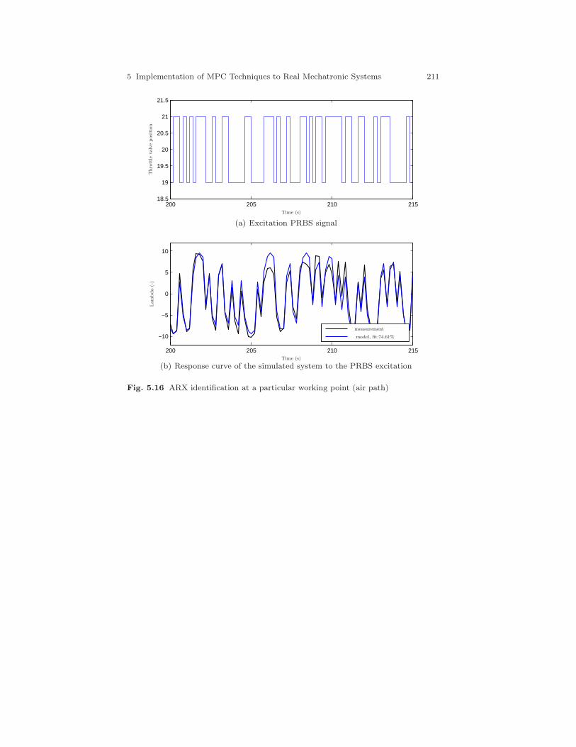
5 Implementation of MPC Techniques to Real Mechatronic Systems 211
200 205 210 21518.5
19
19.5
20
20.5
21
21.5
Throttle
valveposition
Time (s)
(a) Excitation PRBS signal
200 205 210 215
−10
−5
0
5
10
Lambda(-)
Time (s)
measurement
model, fit:74.61%
(b) Response curve of the simulated system to the PRBS excitation
Fig. 5.16 ARX identification at a particular working point (air path)
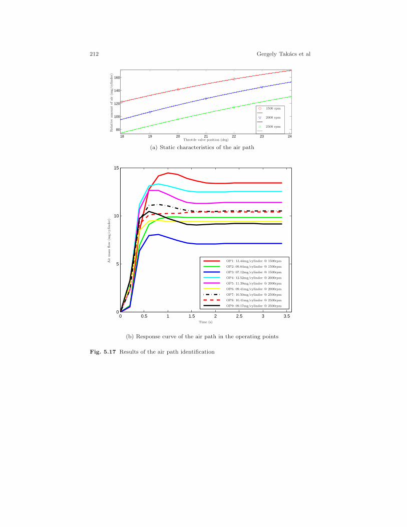
212 Gergely Takacs et al
18 19 20 21 22 23 24
80
100
120
140
160
Relativeamountofair
(mg/cy
linder)
Throttle valve position (deg)
1500 rpm
2000 rpm
2500 rpm
(a) Static characteristics of the air path
0 0.5 1 1.5 2 2.5 3 3.50
5
10
15
Air
mass
flow
(mg/cy
linder)
Time (s)
OP1: 13.44mg/cylinder @ 1500rpm
OP2: 09.84mg/cylinder @ 1500rpm
OP3: 07.12mg/cylinder @ 1500rpm
OP4: 12.52mg/cylinder @ 2000rpm
OP5: 11.39mg/cylinder @ 2000rpm
OP6: 09.41mg/cylinder @ 2000rpm
OP7: 10.50mg/cylinder @ 2500rpm
OP8: 10.41mg/cylinder @ 2500rpm
OP9: 09.17mg/cylinder @ 2500rpm
(b) Response curve of the air path in the operating points
Fig. 5.17 Results of the air path identification
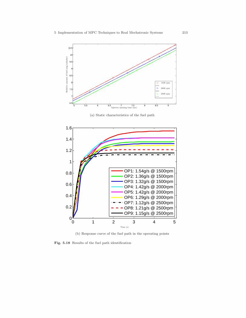
5 Implementation of MPC Techniques to Real Mechatronic Systems 213
5 5.5 6 6.5 7 7.5 8 8.5 96.5
7
7.5
8
8.5
9
9.5
10
10.5
Relativeamountoffuel
(mg/cy
linder)
Injector opening time (ms)
1500 rpm
2000 rpm
2500 rpm
(a) Static characteristics of the fuel path
0 1 2 3 4 50
0.2
0.4
0.6
0.8
1
1.2
1.4
1.6
OP1: 1.54g/s @ 1500rpmOP2: 1.36g/s @ 1500rpmOP3: 1.32g/s @ 1500rpmOP4: 1.42g/s @ 2000rpmOP5: 1.42g/s @ 2000rpmOP6: 1.29g/s @ 2000rpmOP7: 1.12g/s @ 2500rpmOP8: 1.21g/s @ 2500rpmOP9: 1.15g/s @ 2500rpm
Time (s)
(b) Response curve of the fuel path in the operating points
Fig. 5.18 Results of the fuel path identification
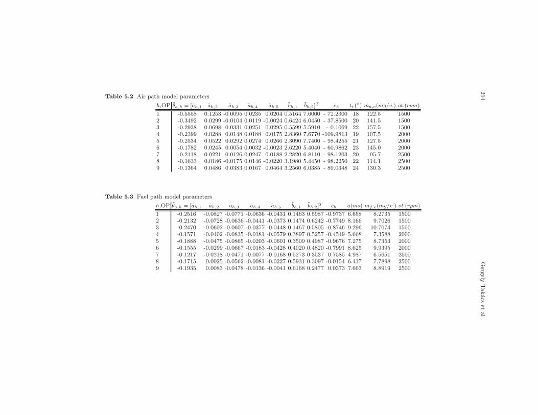
214
Gerg
elyTakacs
etal
Table 5.2 Air path model parameters
h,OP θa,h = [ah,1 ah,2 ah,3 ah,4 ah,5 bh,1 bh,2]T ch tr() ma,e(mg/v.) ot.(rpm)
1 -0.5558 0.1253 -0.0095 0.0235 0.0204 0.5164 7.6000 - 72.2300 18 122.5 15002 -0.3492 0.0299 -0.0104 0.0119 -0.0024 0.6424 6.0450 - 37.8500 20 141.5 15003 -0.2938 0.0698 0.0331 0.0251 0.0295 0.5599 5.5910 - 0.1069 22 157.5 15004 -0.2399 0.0288 0.0148 0.0188 0.0175 2.8360 7.6770 -109.9813 19 107.5 20005 -0.2534 0.0522 0.0292 0.0274 0.0266 2.3090 7.7400 - 98.4255 21 127.5 20006 -0.1782 0.0245 0.0054 0.0032 -0.0023 2.6220 5.4040 - 60.9862 23 145.0 20007 -0.2118 0.0221 0.0126 0.0247 0.0188 2.2820 6.8110 - 98.1203 20 95.7 25008 -0.1633 0.0186 -0.0175 0.0146 -0.0220 3.1980 5.4450 - 98.2250 22 114.1 25009 -0.1364 0.0486 0.0383 0.0167 0.0464 3.2560 6.0385 - 89.0348 24 130.3 2500
Table 5.3 Fuel path model parameters
h,OP θa,h = [ah,1 ah,2 ah,3 ah,4 ah,5 bh,1 bh,2]T ch u(ms) mf,e(mg/v.) ot.(rpm)
1 -0.2516 -0.0827 -0.0771 -0.0636 -0.0431 0.1463 0.5987 -0.9737 6.658 8.2735 15002 -0.2132 -0.0728 -0.0636 -0.0441 -0.0373 0.1474 0.6242 -0.7749 8.166 9.7026 15003 -0.2470 -0.0602 -0.0607 -0.0377 -0.0448 0.1467 0.5805 -0.8746 9.296 10.7074 15004 -0.1571 -0.0402 -0.0835 -0.0181 -0.0579 0.3897 0.5257 -0.4549 5.668 7.3588 20005 -0.1888 -0.0475 -0.0865 -0.0203 -0.0601 0.3509 0.4987 -0.9676 7.275 8.7353 20006 -0.1555 -0.0299 -0.0667 -0.0183 -0.0428 0.4020 0.4820 -0.7991 8.625 9.9395 20007 -0.1217 -0.0218 -0.0471 -0.0077 -0.0168 0.5273 0.3537 0.7585 4.987 6.5651 25008 -0.1715 0.0025 -0.0562 -0.0081 -0.0227 0.5931 0.3097 -0.0154 6.437 7.7898 25009 -0.1935 0.0083 -0.0478 -0.0136 -0.0041 0.6168 0.2477 0.0373 7.663 8.8919 2500
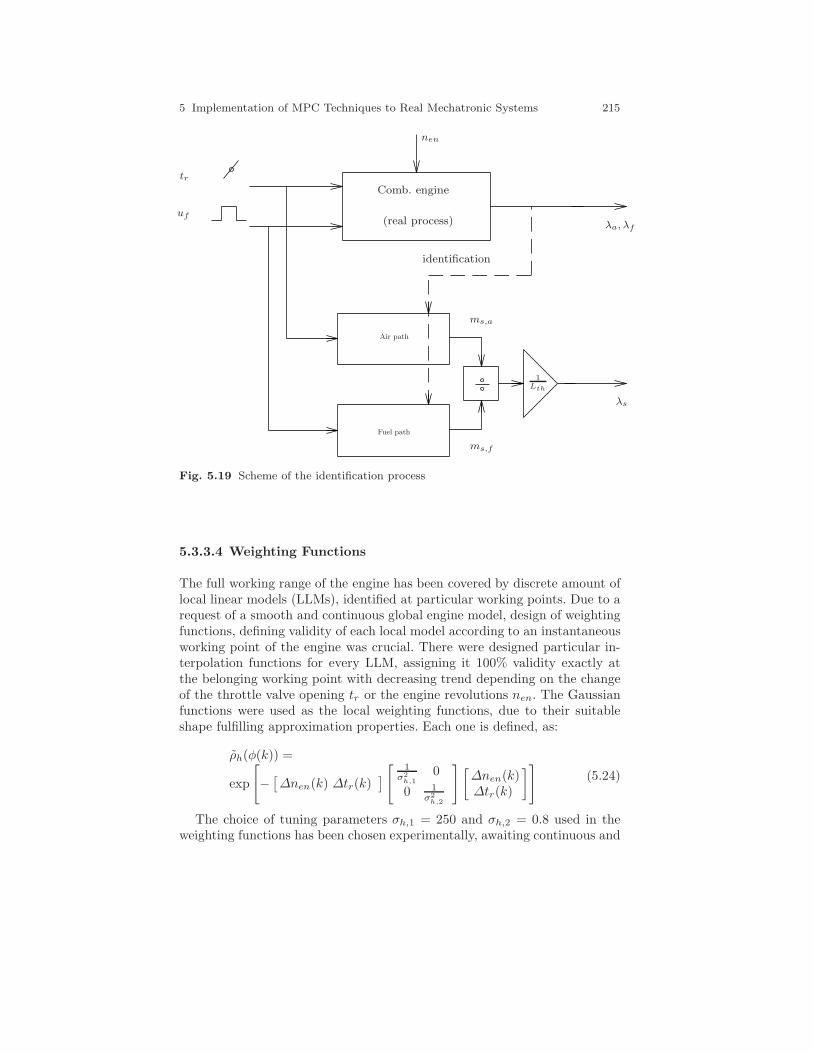
5 Implementation of MPC Techniques to Real Mechatronic Systems 215
nen
tr
uf
Comb. engine
(real process) λa, λf
identification
ms,a
Air path
Fuel path
ms,f
1
Lth
λs
Fig. 5.19 Scheme of the identification process
5.3.3.4 Weighting Functions
The full working range of the engine has been covered by discrete amount oflocal linear models (LLMs), identified at particular working points. Due to arequest of a smooth and continuous global engine model, design of weightingfunctions, defining validity of each local model according to an instantaneousworking point of the engine was crucial. There were designed particular in-terpolation functions for every LLM, assigning it 100% validity exactly atthe belonging working point with decreasing trend depending on the changeof the throttle valve opening tr or the engine revolutions nen. The Gaussianfunctions were used as the local weighting functions, due to their suitableshape fulfilling approximation properties. Each one is defined, as:
ρh(φ(k)) =
exp
[−[∆nen(k) ∆tr(k)
][ 1
σ2h,1
0
0 1σ2h,2
][∆nen(k)∆tr(k)
]](5.24)
The choice of tuning parameters σh,1 = 250 and σh,2 = 0.8 used in theweighting functions has been chosen experimentally, awaiting continuous and
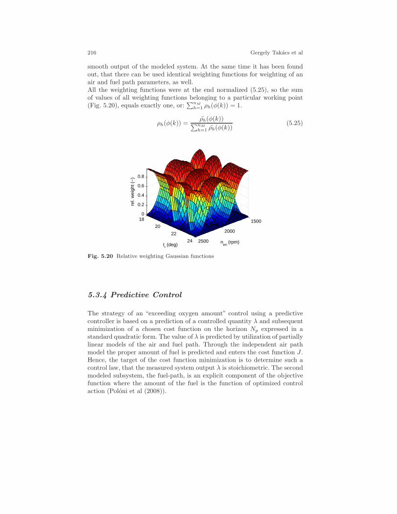
216 Gergely Takacs et al
smooth output of the modeled system. At the same time it has been foundout, that there can be used identical weighting functions for weighting of anair and fuel path parameters, as well.All the weighting functions were at the end normalized (5.25), so the sumof values of all weighting functions belonging to a particular working point(Fig. 5.20), equals exactly one, or:
∑nM
h=1 ρh(φ(k)) = 1.
ρh(φ(k)) =ρh(φ(k))∑nM
h=1 ρh(φ(k))(5.25)
1500
2000
2500
18
20
22
24
0
0.2
0.4
0.6
0.8
nen
(rpm)tr (deg)
rel.
wei
ght (
−)
Fig. 5.20 Relative weighting Gaussian functions
5.3.4 Predictive Control
The strategy of an “exceeding oxygen amount” control using a predictivecontroller is based on a prediction of a controlled quantity λ and subsequentminimization of a chosen cost function on the horizon Np expressed in astandard quadratic form. The value of λ is predicted by utilization of partiallylinear models of the air and fuel path. Through the independent air pathmodel the proper amount of fuel is predicted and enters the cost function J .Hence, the target of the cost function minimization is to determine such acontrol law, that the measured system output λ is stoichiometric. The secondmodeled subsystem, the fuel-path, is an explicit component of the objectivefunction where the amount of the fuel is the function of optimized controlaction (Poloni et al (2008)).
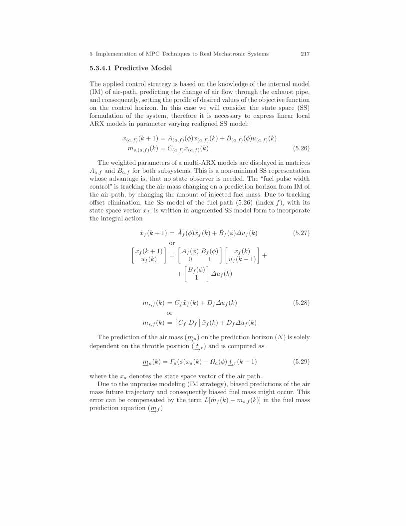
5 Implementation of MPC Techniques to Real Mechatronic Systems 217
5.3.4.1 Predictive Model
The applied control strategy is based on the knowledge of the internal model(IM) of air-path, predicting the change of air flow through the exhaust pipe,and consequently, setting the profile of desired values of the objective functionon the control horizon. In this case we will consider the state space (SS)formulation of the system, therefore it is necessary to express linear localARX models in parameter varying realigned SS model:
x(a,f)(k + 1) = A(a,f)(φ)x(a,f)(k) +B(a,f)(φ)u(a,f)(k)
ms,(a,f)(k) = C(a,f)x(a,f)(k) (5.26)
The weighted parameters of a multi-ARX models are displayed in matricesAa,f and Ba,f for both subsystems. This is a non-minimal SS representationwhose advantage is, that no state observer is needed. The “fuel pulse widthcontrol” is tracking the air mass changing on a prediction horizon from IM ofthe air-path, by changing the amount of injected fuel mass. Due to trackingoffset elimination, the SS model of the fuel-path (5.26) (index f ), with itsstate space vector xf , is written in augmented SS model form to incorporatethe integral action
xf (k + 1) = Af (φ)xf (k) + Bf (φ)∆uf (k) (5.27)
or[xf (k + 1)uf (k)
]=
[Af (φ) Bf (φ)
0 1
] [xf (k)
uf(k − 1)
]+
+
[Bf (φ)
1
]∆uf(k)
ms,f (k) = Cf xf (k) +Df∆uf (k) (5.28)
or
ms,f (k) =[Cf Df
]xf (k) +Df∆uf (k)
The prediction of the air mass (m−→a) on the prediction horizon (N) is solely
dependent on the throttle position ( t−→r) and is computed as
m−→a(k) = Γa(φ)xa(k) +Ωa(φ) t−→r(k − 1) (5.29)
where the xa denotes the state space vector of the air path.Due to the unprecise modeling (IM strategy), biased predictions of the air
mass future trajectory and consequently biased fuel mass might occur. Thiserror can be compensated by the term L[mf (k) −ms,f (k)] in the fuel massprediction equation (m−→f )
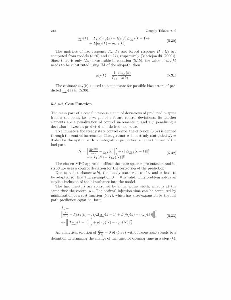
218 Gergely Takacs et al
m−→f (k) = Γf (φ)xf (k) +Ωf (φ)∆ u−→f (k − 1)+
+ L[mf(k)−ms,f (k)](5.30)
The matrices of free response Γa, Γf and forced response Ωa, Ωf arecomputed from models (5.26) and (5.27), respectively (Maciejowski (2000)).Since there is only λ(k) measurable in equation (5.15), the value of ma(k)needs to be substituted using IM of the air-path, then
mf (k) =1
Lth
ms,a(k)
λ(k)(5.31)
The estimate mf (k) is used to compensate for possible bias errors of pre-dicted m−→f (k) in (5.30).
5.3.4.2 Cost Function
The main part of a cost function is a sum of deviations of predicted outputsfrom a set point, i.e. a weight of a future control deviations. Its anotherelements are a penalization of control increments r; and a p penalizing adeviation between a predicted and desired end state.
To eliminate a the steady state control error, the criterion (5.32) is definedthrough the control increments. That guarantees in a steady state, that Jλ =0 also for the system with no integration properties, what is the case of thefuel path
Jλ =∥∥∥
m−→a(k)
Lth− m−→f (k)
∥∥∥2
2+ r‖∆ u−→f (k − 1)‖22
+p‖xf (N)− xf,r(N)‖22(5.32)
The chosen MPC approach utilizes the state space representation and itsstructure uses a control deviation for the correction of the prediction.
Due to a disturbance d(k), the steady state values of u and x have tobe adapted so, that the assumption J = 0 is valid. This problem solves anexplicit inclusion of the disturbance into the model.
The fuel injectors are controlled by a fuel pulse width, what is at thesame time the control uf . The optimal injection time can be computed byminimization of a cost function (5.32), which has after expansion by the fuelpath prediction equation, form:
Jλ =∥∥∥m−→a
Lth− Γf xf (k) +Ωf∆ u−→f (k − 1) + L[mf(k)−ms,f (k)]
∥∥∥2
2
+r∥∥∥∆ u−→f (k − 1)
∥∥∥2
2+ p‖xf (N)− xf,r(N)‖22
(5.33)
An analytical solution of dJλ
∆u−→= 0 of (5.33) without constraints leads to a
definition determining the change of fuel injector opening time in a step (k),
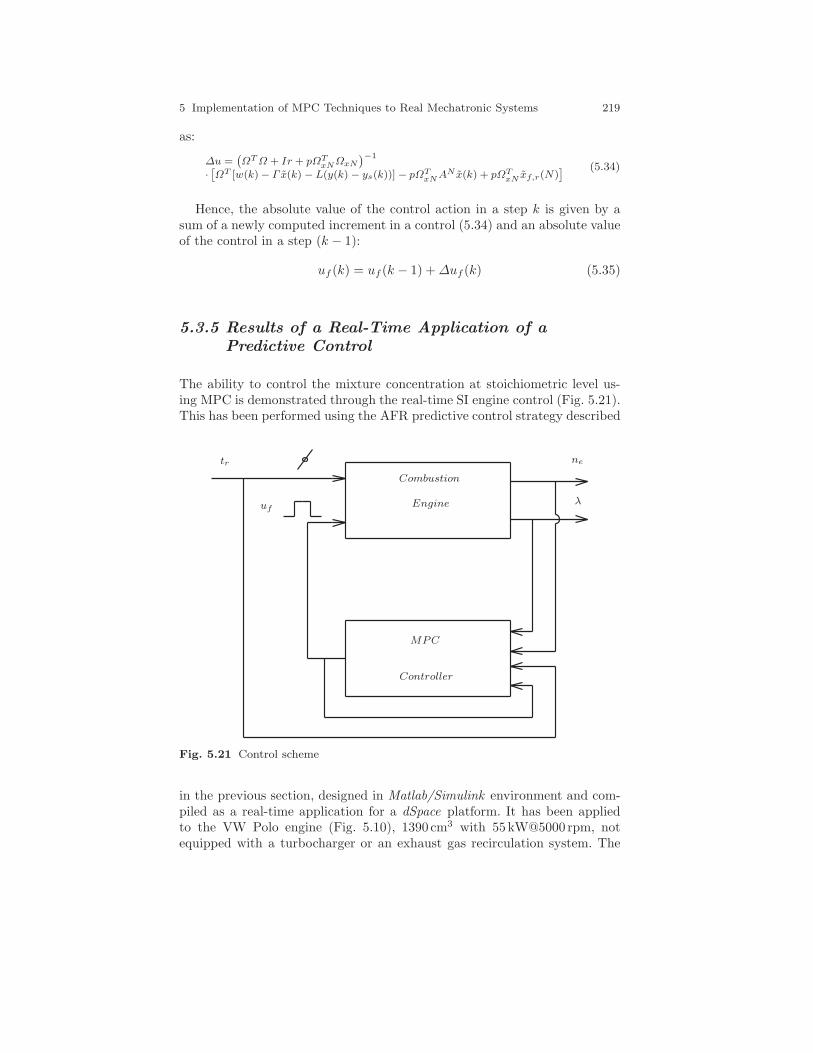
5 Implementation of MPC Techniques to Real Mechatronic Systems 219
as:
∆u =(
ΩTΩ + Ir + pΩTxNΩxN
)
−1
·[
ΩT [w(k)− Γ x(k) − L(y(k) − ys(k))]− pΩTxN
AN x(k) + pΩTxN
xf,r(N)] (5.34)
Hence, the absolute value of the control action in a step k is given by asum of a newly computed increment in a control (5.34) and an absolute valueof the control in a step (k − 1):
uf (k) = uf (k − 1) +∆uf (k) (5.35)
5.3.5 Results of a Real-Time Application of aPredictive Control
The ability to control the mixture concentration at stoichiometric level us-ing MPC is demonstrated through the real-time SI engine control (Fig. 5.21).This has been performed using the AFR predictive control strategy described
Combustion
Engine
MPC
Controller
tr
uf
ne
λ
Fig. 5.21 Control scheme
in the previous section, designed in Matlab/Simulink environment and com-piled as a real-time application for a dSpace platform. It has been appliedto the VW Polo engine (Fig. 5.10), 1390 cm3 with 55kW@5000 rpm, notequipped with a turbocharger or an exhaust gas recirculation system. The
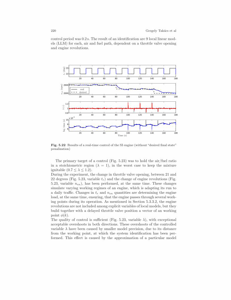
220 Gergely Takacs et al
control period was 0.2 s. The result of an identification are 9 local linear mod-els (LLM) for each, air and fuel path, dependent on a throttle valve openingand engine revolutions.
20 40 60 80 100 120 140 160 180
22
23
20 40 60 80 100 120 140 160 180
2000
2500
20 40 60 80 100 120 140 160 1800.8
1
1.2
20 40 60 80 100 120 140 160 180
6
8
10x 10
−3
t r(d
eg)
nen(rpm)
λ(-)
Inj.time(s)
Time (s)
real
desired
Fig. 5.22 Results of a real-time control of the SI engine (without“desired final state”penalization)
The primary target of a control (Fig. 5.23) was to hold the air/fuel ratioin a stoichiometric region (λ = 1), in the worst case to keep the mixtureignitable (0.7 ≤ λ ≤ 1.2).During the experiment, the change in throttle valve opening, between 21 and22 degrees (Fig. 5.23, variable tr) and the change of engine revolutions (Fig.5.23, variable nen), has been performed, at the same time. These changessimulate varying working regimes of an engine, which is adapting its run toa daily traffic. Changes in tr and nen quantities are determining the engineload, at the same time, ensuring, that the engine passes through several work-ing points during its operation. As mentioned in Section 5.3.3.2, the enginerevolutions are not included among explicit variables of local models, but theybuild together with a delayed throttle valve position a vector of an workingpoint φ(k).The quality of control is sufficient (Fig. 5.23, variable λ), with exceptionalacceptable overshoots in both directions. These overshoots of the controlledvariable λ have been caused by smaller model precision, due to its distancefrom the working point, at which the system identification has been per-formed. This effect is caused by the approximation of a particular model
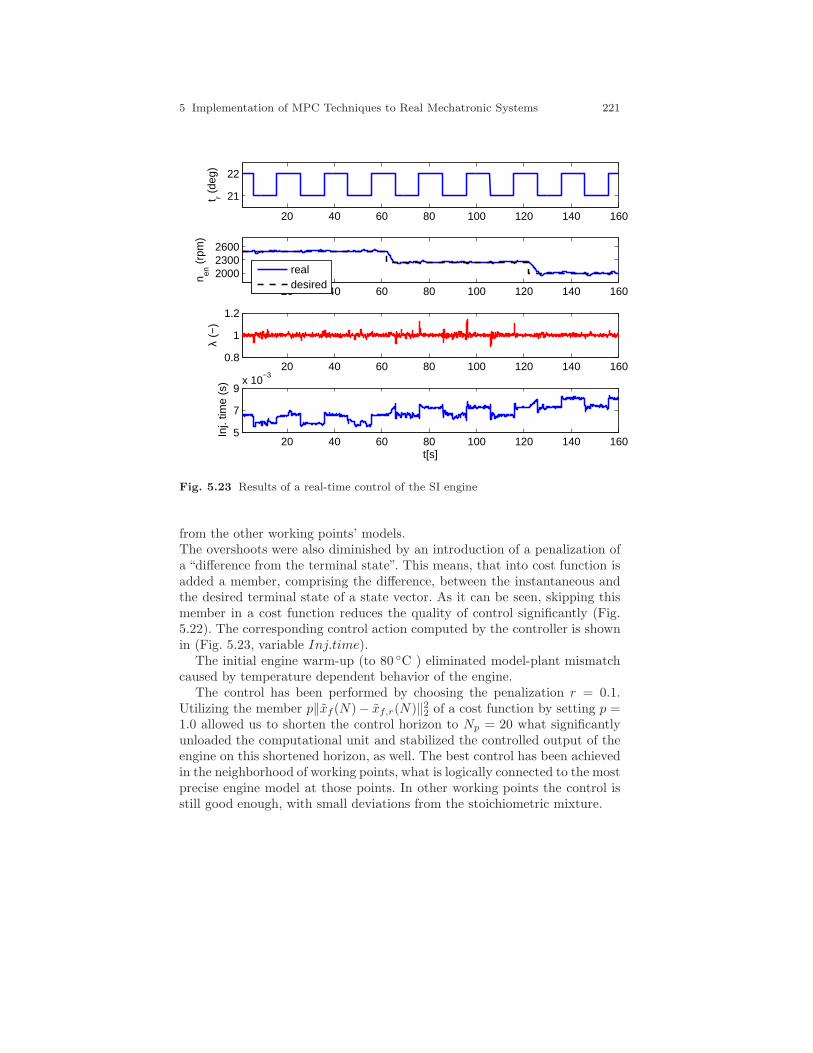
5 Implementation of MPC Techniques to Real Mechatronic Systems 221
20 40 60 80 100 120 140 160
21
22
t r (de
g)
20 40 60 80 100 120 140 160
200023002600
n en (
rpm
)
realdesired
20 40 60 80 100 120 140 1600.8
1
1.2
λ (−
)
20 40 60 80 100 120 140 1605
7
9x 10
−3
Inj.
time
(s)
t[s]
Fig. 5.23 Results of a real-time control of the SI engine
from the other working points’ models.The overshoots were also diminished by an introduction of a penalization ofa “difference from the terminal state”. This means, that into cost function isadded a member, comprising the difference, between the instantaneous andthe desired terminal state of a state vector. As it can be seen, skipping thismember in a cost function reduces the quality of control significantly (Fig.5.22). The corresponding control action computed by the controller is shownin (Fig. 5.23, variable Inj.time).
The initial engine warm-up (to 80 C ) eliminated model-plant mismatchcaused by temperature dependent behavior of the engine.
The control has been performed by choosing the penalization r = 0.1.Utilizing the member p‖xf(N)− xf,r(N)‖22 of a cost function by setting p =1.0 allowed us to shorten the control horizon to Np = 20 what significantlyunloaded the computational unit and stabilized the controlled output of theengine on this shortened horizon, as well. The best control has been achievedin the neighborhood of working points, what is logically connected to the mostprecise engine model at those points. In other working points the control isstill good enough, with small deviations from the stoichiometric mixture.
222 Gergely Takacs et al
5.3.6 Conclusion
Considering the preliminary results from the real-time experiments at theengine, it can be concluded, that the idea of the AFR model predictive con-trol based on local ARX models is suitable and applicable for the SI enginecontrol. Proposed flexible design of a predictive controller offers easy tuningpossibilities, extension of the global engine model to other working regimesof the engine and implementation of constraints. This fact also indicates thenext project step, which is the overshoot elimination in the λ - control by theidentification of wider net of “local engine models”.
Acknowledgements The authors gratefully acknowledge the financial support grantedby the Slovak Research and Development Agency under the contracts LPP-0096-07,LPP-0075-09 and LPP-0118-09. This research is also supported by the grant fromIceland, Liechtenstein and Norway through the EEA Financial Mechanism and theNorwegian Financial Mechanism. This grant is co-financed from the state budget ofthe Slovak Republic.
References
Anstee R (2006) The Newton-Rhapson Method. Lecture notesArsie I, Iorio SD, Noschese G, Pianese C, Sorrentino M (2008) Optimal air-fuel ratio.
dSpace Magazine (1):20–23Bengtsson J, Strandh P, Johansson R, Tunestal P, Johansson B (2007) Hybrid model-
ing of homogenous charge compression ignition (HCCI) engine dynamics -a survey.International journal of control 80(11):1814–1847
Cannon M, Kouvaritakis B (2005) Optimizing Prediction Dynamics for Robust MPC.IEEE Transactions on Automatic Control 50(11):1892–1597
Chen H, Allgover F (1998) A quasi-infinite horizon nonlinear model predictive controlscheme with guaranteed stability. Automatica 34(10):1205–1217
Dong X, Meng G, Peng J (2006) Vibration control of piezoelectric smart structuresbased on system identification technique: Numerical simulation and experimentalstudy. Journal of Sound and Vibration 273:680–693
Ferreau H (2006) An online active set strategy for fast solution of parametric quadraticprograms with applications to predictive engine control. Master’s thesis, Universityof Heidelberg
Ferreau H, Bock H, Diehl M (2008) An online active set strategy to overcome thelimitations of explicit mpc. International Journal of Robust and Nonlinear Control18(8):816–830
dSPACE GmbH (2009) HelpDesk ApplicationHou Z (2007) Air fuel ratio control for gasoline engine using neural network multi-step
predictive model. 3rd international conference on intelligent computing, Qingdao,China
Kouvaritakis B, Rossiter J, Schuurmans J (2000) Efficient robust predictive control.IEEE Transactions on Automatic Control 45(8):1545–1549
Kouvaritakis B, Cannon M, Rossiter J (2002) Who needs QP for linear MPC anyway?Automatica 38:879–884
5 Implementation of MPC Techniques to Real Mechatronic Systems 223
Kvasnica M, Grieder P, Baotic M (2004) Multi-Parametric Toolbox (MPT). Online,available: http://control.ee.ethz.ch/
Kvasnica M, Grieder P, Baotic M, Christophersen FJ (2006) Multi-Parametric Tool-box (MPT). Extended documentation
Lara A, Burch JC, Schloss JM, Sadek IS, Adali S (2003) Piezo patch sensor/actuatorcontrol of the vibrations of a cantilever under axial load. Composite Structures62:423–428
L ofberg J (2004) YALMIP: A toolbox for modeling and optimization in MATLAB.In: Proceedings of the CACSD Conference, Taipei, Taiwan
Lorini G, Miotti A, Scattolini R (2006) Modeling, simulation and predictive controlof a spark ignition engine. In: Predimot (ed) Predictive control of combustionengines, TRAUNER Druck GmbH & CoKG, pp 39–55
Maciejowski J (2002) Predictive Control with Constraints, 1st edn. Prentice HallMaciejowski JM (2000) Predictive control with constraints. University of CambridgeMao X, Wang D, Xiao W, Liu Z, Wang J, Tang H (2009) Lean limit and emissions
improvement for a spark-ignited natural gas engine using a generalized predictivecontrol (GPC)-based air/fuel ratio controller. Energy & Fuels (23):6026–6032
MathWorks T (2007) Matlab signal processing blockset v6.6 (r2007b). Software.Mayne DQ, Rawlings JB, Rao CV, Scokaert POM (2000a) Constrained model pre-
dictive control: Stability and optimality. Automatica 36:789–814Mayne DQ, Rawlings JB, Rao CV, Scokaert POM (2000b) Constrained model pre-
dictive control: Stability and optimality. Automatica (36):789–814Murray-Smith R, Johanssen TA (1997) Multiple model approaches to modelling and
control. Taylor & FrancisMuske KR, Jones JCP (2006) A model-based SI engine air fuel ratio controller. Amer-
ican Control Conference, Minneapolis, USAPoloni T, Rohal’-Ilkiv B, Johansen TA (2007) Multiple ARX model-based air-fuel
ratio predictive control for SI engines. In: IFAC Workshop on advanced fuzzy andneural control, Valenciennes, France, conference paper MO5-3
Poloni T, Johansen TA, Rohal’-Ilkiv B (2008) Identification and modeling of air-fuel ratio dynamics of a gasoline combustion engine with weighted arx modelnetwork. Transaction of the ASME (Journal of Dynamic Systems, Measurement,and Control) 130(6), 061009
Preumont A (2002) Vibration Control of Active Structures, 2nd edn. Kluwer Aca-demic Publishers
Rossiter JA (2003) Model-based predictive control: a practical approach, 1st edn.CRC Press LCC
Song G, Qiao PZ, Bibienda WK, Zhou GP (2002) Active vibration damping of com-posite beam using smart sensors and actuators. Journal of Aerospace Engineering15(3):97–103
Sturm JF (1999) Using SeDuMi 1.02, a MATLAB toolbox for optimization oversymmetric cones. Optimization Methods and Software - Special issue on InteriorPoint Methods 11-12:625–653
Takacs G, Rohal’-Ilkiv B (2009) MPC with guaranteed stability and constraint feasi-bility on flexible vibrating active structures: a comparative study. In: Proceedingsof The eleventh IASTED International Conference on Control and Applications,Cambridge, United Kingdom.
Wills AG, Bates D, Fleming AJ, Ninness B, Moheimani SOR (2008) Model predictivecontrol applied to constraint handling in active noise and vibration control. IEEETransactions on Control Systems Technology 16(1):3–12
Zeman J, Rohal-Ilkiv B (2003) Robust min-max model predictive control of linearsystems with constraints. IEEE International Conference on Industrial Technology,pp 930 – 935

224 Gergely Takacs et al
Zhai YJ, Yu DL (2009) Neural network model-based automotive engine air/fuel ratiocontrol and robustness evaluation. Engineering Applications of Artificial Intelli-gence (22):171U180
Zhai YJ, Ding-WenYu, Hong-YuGuo, DLYu (2010) Robust air/fuel ratio control withadaptive DRNN model and AD tuning. Engineering Applications of Artificial In-telligence (23):283–289

5 Implementation of MPC Techniques to Real Mechatronic Systems 225
Comments – Remarks

226 Gergely Takacs et al
Comments – Remarks

5 Implementation of MPC Techniques to Real Mechatronic Systems 227
Comments – Remarks

228 Gergely Takacs et al
Comments – Remarks
Chapter 6
Laboratory Model of Coupled Tanks
Vladimır Zilka and Mikulas Huba
Abstract This chapter gives introduction into work with frequently usedhydro-system of coupled tanks. The chapter explains analytical modellingfor one and two-level systems of coupled tanks, including the experimentalidentification of system’s parameters and sensor’s calibration.
6.1 Introduction
To be able to use their knowledge in solving practical tasks, for graduates it isimportant to develope skills in applying control theory related to linear andnon linear systems to real plants control. This may be just partially achievedby computer simulations and the feedback received in such a way is nevercomplete. Therefore, it is important to acquire already during the universitystudies some practice and experience related competences in designing andtesting of controllers on real systems.
Due to the simple manipulation, easily understandable and observable pro-cesses and their time constants, one of many systems used at universities fre-quently as pedagogical instruments in control education the system of coupledtanks has to be mentioned. The theoretical design of controllers included inthis publication comprehends two basic configurations: control of one, or oftwo coupled tanks. In considering coupled tanks, one of possible configura-tions is the coupling in series with interaction, when the liquid’s level in oneof the tanks influences the other tank’s liquid’s level as the liquid may flow
Vladimır ZilkaFaculty of Electrical Engineering and Information Technology, Slovak University ofTechnology in Bratislava, e-mail: [email protected]
Mikulas HubaFaculty of Electrical Engineering and Information Technology, Slovak University ofTechnology in Bratislava, e-mail: [email protected]
229
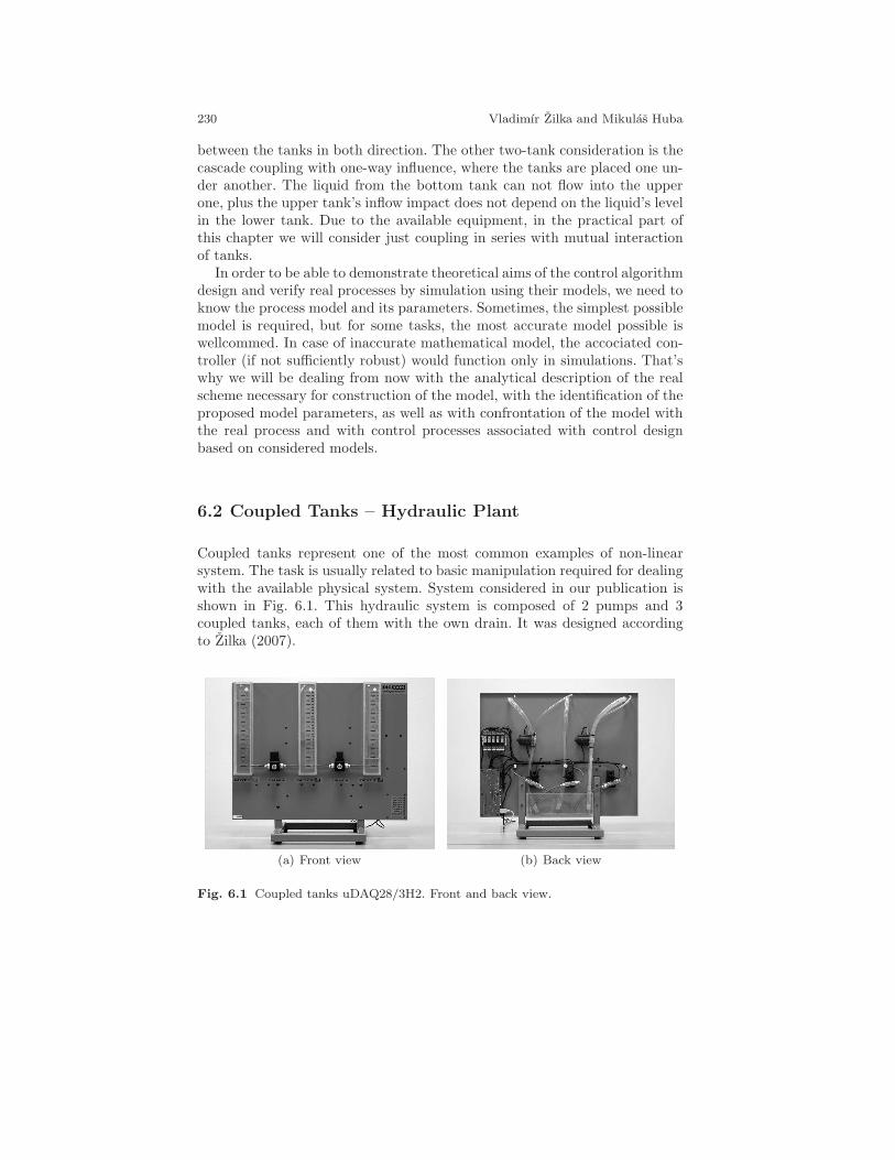
230 Vladimır Zilka and Mikulas Huba
between the tanks in both direction. The other two-tank consideration is thecascade coupling with one-way influence, where the tanks are placed one un-der another. The liquid from the bottom tank can not flow into the upperone, plus the upper tank’s inflow impact does not depend on the liquid’s levelin the lower tank. Due to the available equipment, in the practical part ofthis chapter we will consider just coupling in series with mutual interactionof tanks.
In order to be able to demonstrate theoretical aims of the control algorithmdesign and verify real processes by simulation using their models, we need toknow the process model and its parameters. Sometimes, the simplest possiblemodel is required, but for some tasks, the most accurate model possible iswellcommed. In case of inaccurate mathematical model, the accociated con-troller (if not sufficiently robust) would function only in simulations. That’swhy we will be dealing from now with the analytical description of the realscheme necessary for construction of the model, with the identification of theproposed model parameters, as well as with confrontation of the model withthe real process and with control processes associated with control designbased on considered models.
6.2 Coupled Tanks – Hydraulic Plant
Coupled tanks represent one of the most common examples of non-linearsystem. The task is usually related to basic manipulation required for dealingwith the available physical system. System considered in our publication isshown in Fig. 6.1. This hydraulic system is composed of 2 pumps and 3coupled tanks, each of them with the own drain. It was designed accordingto Zilka (2007).
(a) Front view (b) Back view
Fig. 6.1 Coupled tanks uDAQ28/3H2. Front and back view.
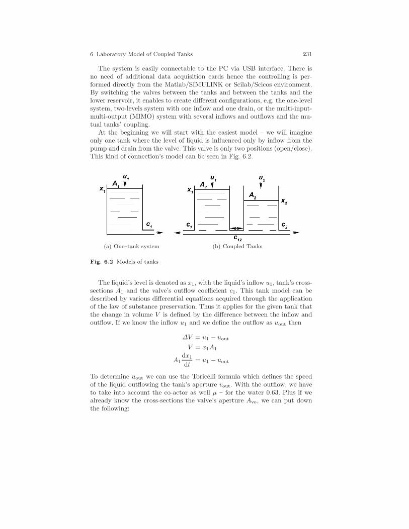
6 Laboratory Model of Coupled Tanks 231
The system is easily connectable to the PC via USB interface. There isno need of additional data acquisition cards hence the controlling is per-formed directly from the Matlab/SIMULINK or Scilab/Scicos environment.By switching the valves between the tanks and between the tanks and thelower reservoir, it enables to create different configurations, e.g. the one-levelsystem, two-levels system with one inflow and one drain, or the multi-input-multi-output (MIMO) system with several inflows and outflows and the mu-tual tanks’ coupling.
At the beginning we will start with the easiest model – we will imagineonly one tank where the level of liquid is influenced only by inflow from thepump and drain from the valve. This valve is only two positions (open/close).This kind of connection’s model can be seen in Fig. 6.2.
(a) One–tank system (b) Coupled Tanks
Fig. 6.2 Models of tanks
The liquid’s level is denoted as x1, with the liquid’s inflow u1, tank’s cross-sections A1 and the valve’s outflow coefficient c1. This tank model can bedescribed by various differential equations acquired through the applicationof the law of substance preservation. Thus it applies for the given tank thatthe change in volume V is defined by the difference between the inflow andoutflow. If we know the inflow u1 and we define the outflow as uout then
∆V = u1 − uout
V = x1A1
A1dx1
dt= u1 − uout
To determine uout we can use the Toricelli formula which defines the speedof the liquid outflowing the tank’s aperture vout. With the outflow, we haveto take into account the co-actor as well µ – for the water 0.63. Plus if wealready know the cross-sections the valve’s aperture Avo, we can put downthe following:
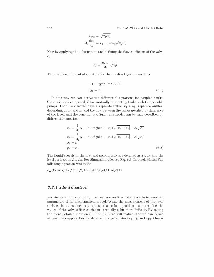
232 Vladimır Zilka and Mikulas Huba
vout =√2gx1
A1dx1
dt= u1 − µAvo
√2gx1
Now by applying the substitution and defining the flow coefficient of the valvec1
c1 =µAvo
A1
√2g
The resulting differential equation for the one-level system would be
x1 =1
A1u1 − c1
√x1
y1 = x1 (6.1)
In this way we can derive the differential equations for coupled tanks.System is then composed of two mutually interacting tanks with two possiblepumps. Each tank would have a separate inflow u1 a u2, separate outflowdepending on x1 and x2 and the flow between the tanks specified by differenceof the levels and the constant c12. Such tank model can be then described bydifferential equations
x1 =1
A1u1 − c12 sign(x1 − x2)
√|x1 − x2| − c1
√x1
x2 =1
A2u2 + c12 sign(x1 − x2)
√|x1 − x2| − c2
√x2
y1 = x1
y2 = x2 (6.2)
The liquid’s levels in the first and second tank are denoted as x1, x2 and thelevel surfaces as A1, A2. For Simulink model see Fig. 6.3. In block MatlabFcnfollowing equation was made
c_12sign(u(1)-u(2))sqrt(abs(u(1)-u(2)))
6.2.1 Identification
For simulating or controlling the real system it is indispensable to know allparameters of its mathematical model. While the measurement of the levelsurfaces in tanks does not represent a serious problem, to determine thevalues of the valve’s flow coeficient is usually a bit more difficult. By takingthe more detailed view on (6.1) or (6.2) we will realize that we can defineat least two approaches for determining parameters c1, c2 and c12. One is
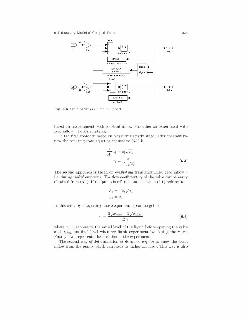
6 Laboratory Model of Coupled Tanks 233
Fig. 6.3 Coupled tanks - Simulink model.
based on measurement with constant inflow, the other on experiment withzero inflow – tank’s emptying.
In the first approach based on measuring steady state under constant in-flow the resulting state equation reduces to (6.1) is
1
A1u1 = c1
√x1
c1 =u1
A1√x1
(6.3)
The second approach is based on evaluating transients under zero inflow –i.e. during tanks’ emptying. The flow coefficient c1 of the valve can be easilyobtained from (6.1). If the pump is off, the state equation (6.1) reduces to
x1 = −c1√x1
y1 = x1
In this case, by integrating above equation, c1 can be get as
c1 =2√x1init − 2
√x1final
∆t1(6.4)
where x1init represents the initial level of the liquid before opening the valveand x1final its final level when we finish experiment by closing the valve.Finally, ∆t1 represents the duration of the experiment.
The second way of determination c1 does not require to know the exactinflow from the pump, which can leads to higher accuracy. This way is also
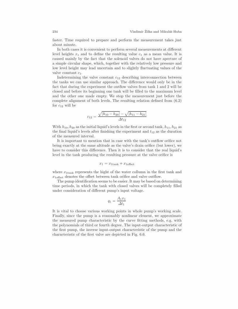
234 Vladimır Zilka and Mikulas Huba
faster. Time required to prepare and perform the measurement takes justabout minute.
In both cases it is convenient to perform several measurements at differentlevel heights x1 and to define the resulting value c1 as a mean value. It iscaused mainly by the fact that the solenoid valves do not have aperture ofa simple circular shape, which, together with the relatively low pressure andlow level height may lead uncertain and to slightly fluctuating values of thevalve constant c1.
Indetermining the valve constant c12 describing interconnection betweenthe tanks we can use similar approach. The difference would only be in thefact that during the experiment the outflow valves from tank 1 and 2 will beclosed and before its beginning one tank will be filled to the maximum leveland the other one made empty. We stop the measurement just before thecomplete alignment of both levels. The resulting relation defined from (6.2)for c12 will be
c12 =
√|h10 − h20| −
√|h11 − h21|
∆t12
With h10, h20 as the initial liquid’s levels in the first or second tank, h11, h21 asthe final liquid’s levels after finishing the experiment and t12 as the durationof the measured interval.
It is important to mention that in case with the tank’s outflow orifice notbeing exactly at the same altitude as the valve’s drain orifice (but lower), wehave to consider this difference. Then it is to consider that the real liquid’slevel in the tank producing the resulting pressure at the valve orifice is
x1 = x1tank + x1offset
where x1tank represents the hight of the water collumn in the first tank andx1offset denotes the offset between tank orifice and valve outflow.
The pump identification seems to be easier. It may be based on determiningtime periods, in which the tank with closed valves will be completely filledunder consideration of different pump’s input voltage.
q1 =A1x1
∆t1
It is vital to choose various working points in whole pump’s working scale.Finally, since the pump is a reasonably nonlinear element, we approximatethe measured pump characteristic by the curve fitting methods, e.g. withthe polynomials of third or fourth degree. The input-output characteristic ofthe first pump, the inverse input-output characteristic of the pump and thecharacteristic of the first valve are depicted in Fig. 6.6.
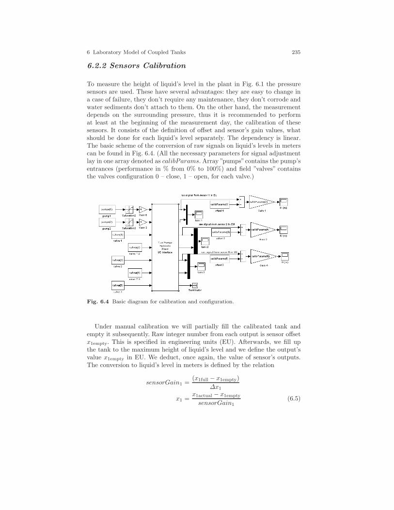
6 Laboratory Model of Coupled Tanks 235
6.2.2 Sensors Calibration
To measure the height of liquid’s level in the plant in Fig. 6.1 the pressuresensors are used. These have several advantages: they are easy to change ina case of failure, they don’t require any maintenance, they don’t corrode andwater sediments don’t attach to them. On the other hand, the measurementdepends on the surrounding pressure, thus it is recommended to performat least at the beginning of the measurement day, the calibration of thesesensors. It consists of the definition of offset and sensor’s gain values, whatshould be done for each liquid’s level separately. The dependency is linear.The basic scheme of the conversion of raw signals on liquid’s levels in meterscan be found in Fig. 6.4. (All the necessary parameters for signal adjustmentlay in one array denoted as calibParams. Array ”pumps”contains the pump’sentrances (performance in % from 0% to 100%) and field ”valves” containsthe valves configuration 0 – close, 1 – open, for each valve.)
Fig. 6.4 Basic diagram for calibration and configuration.
Under manual calibration we will partially fill the calibrated tank andempty it subsequently. Raw integer number from each output is sensor offsetx1empty. This is specified in engineering units (EU). Afterwards, we fill upthe tank to the maximum height of liquid’s level and we define the output’svalue x1empty in EU. We deduct, once again, the value of sensor’s outputs.The conversion to liquid’s level in meters is defined by the relation
sensorGain1 =(x1full − x1empty)
∆x1
x1 =x1actual − x1empty
sensorGain1(6.5)

236 Vladimır Zilka and Mikulas Huba
Here, x1actual is the actual value of liquid’s level in EU, x1empty is the outputin EU at the zero liquid level and x1full is the value of the output in EU atmaximum liquid level and ∆x1 is the height of the maximum liquid level. Forexample, if we know that at the zero level x1empty = 800EU, at the maximumlevel ∆x1 = 0.25m and output 3300EU, for the output 2300EU it holds:
sensorGain1 =3300− 800
0.25= 10000EUm−1
x1 =2300− 800
10000= 0.15m
After the calibration it is suitable to perform identification of system’s pa-rameters. It consists of the estimation of the flow coefficients of valves and ofthe pump’s parameters according to the above-mentioned process.
6.2.3 Automatic Calibration and Identification
The above mentioned procedure of calibration and identification is obviouslytime consuming and also not easy to calculate manually. To perform the suchlong time step-by-step measurements of the pump’s characteristics plus tosave the measured values subsequently after each measurement and evaluatethem afterwards, we have to sacrifice an enormous quantity of time. That’sall is the reason why we developed the software package for automatic iden-tification of system’s individual parameters and for identification of all valveand pump parameters. The control is very easy – only one click is needed toget the required identification in the menu. Menu’s environment can be seenin Fig. 6.5.
As the processes were described in details in the previous chapter, theindividual functionalities will be mentioned now just shortly. At the identifi-cation of the valve 1,2 or 3, the tank is fill up to the height of approximately24.5 cm, then we wait till the liquid’s level is stabilized and the tank is af-terwards emptied to 0.8 cm. (At almost zero level, the valve’s behaviour isstrictly non-linear and as we are not planning to regulate the level under 1 cm,we don’t consider the lowest boundary). The measured values are saved, to-gether with all used constants, into the mat file in the following format:
valveValvenumber-year-month-day-hour-minute-second.mat.For example: valve1-2009-12-20-16-26-43.mat and so on. We don’t
consider the first and the last measurement sample, from the other valueswith the step approximately 1.5 cm – we use each sixth sample, define thevalue c1 as well as the possible offset value of the valve offset1.
At the end we define the mean value of offset and of flow coefficient andwe save those two values together with the time course of emptying intothe valve1, valve2 and valve3.mat. We apply them directly to the proposedmodel, we simulate the emptying and we draw the comparison of simulation
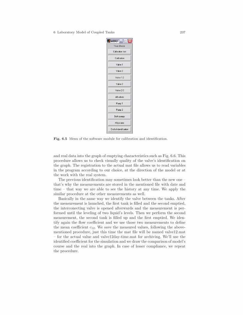
6 Laboratory Model of Coupled Tanks 237
Fig. 6.5 Menu of the software module for calibration and identification.
and real data into the graph of emptying characteristics such as Fig. 6.6. Thisprocedure allows us to check visually quality of the valve’s identification onthe graph. The registration to the actual mat file allows us to read variablesin the program according to our choice, at the direction of the model or atthe work with the real system.
The previous identification may sometimes look better than the new one –that’s why the measurements are stored in the mentioned file with date andtime – that way we are able to see the history at any time. We apply thesimilar procedure at the other measurements as well.
Basically in the same way we identify the valve between the tanks. Afterthe measurement is launched, the first tank is filled and the second emptied,the interconecting valve is opened afterwards and the measurement is per-formed until the leveling of two liquid’s levels. Then we perform the secondmeasurement, the second tank is filled up and the first emptied. We iden-tify again the flow coefficient and we use those two measurements to definethe mean coefficient c12. We save the measured values, following the above-mentioned procedure, just this time the mat file will be named valve12.mat– for the actual value and valve12day-time.mat for archiving. We’ll use theidentified coefficient for the simulation and we draw the comparison of model’scourse and the real into the graph. In case of lesser compliance, we repeatthe procedure.

238 Vladimır Zilka and Mikulas Huba
2 4 6 8 10 120
0.2
0.4
0.6
0.8
1
1.2
1.4
1.6
1.8x 10
−5
pump voltage [V]
pum
p ou
tput
[m3 /s
]
The input − output characteristic of the pump and approximation with 4rd degree polynomial
Real i−o characteristicApproximation
(a) IO characteristic
0 0.2 0.4 0.6 0.8 1 1.2 1.4 1.6 1.8
x 10−5
2
4
6
8
10
12
14
pum
p 1
volta
ge [V
]
pump 1 output [m3/s]
The inverse i−o characteristic of the pump 1 and approximation with 4rd degree polynomial
Real i−o characteristicApproximation
(b) Inverse IO characteristic
0 0.05 0.1 0.15 0.2 0.25
0.018
0.02
0.022
0.024
0.026
0.028
0.03
0.032
0.034
0.036
0.038
level [m]
flow
coe
ffici
ent o
f the
val
ve
The characteristic of the flow coefficient of the valve
identification − 2cm stepsidentification − steady statesapproximation
(c) Determining c1 by the first method
0 5 10 15 20 25 30 35 40 450
0.05
0.1
0.15
0.2
0.25
t [s]
leve
l [m
]
Outflow characteristic for real system and model − tank 1
Real systemSimulation
(d) Determining c1 by the second method
Fig. 6.6 Measured Input-Output pump characteristic and its approximation by the4th degree polynomial and inverse input-output pump characteristic and its approx-imation by the 4th degree polynomial (above). Determination of the valve coefficientc1 with two approaches – comparing the measurement and approximative data fortank 1 (below).
The measurement of pump’s characteristics is more time-consuming. Inorder to achieve the required accuracy, we continue with increasing the pumpinput by the step 3% of the maximal range 100% up to the moment wherethe pump starts slowly to draw the liquid. (In our case it will be around 19– 21 %.) At lower inputs, the pump is not working.
At the beginning of measurement, we empty the tank, and then fill it upby given input up to the fullest state, or during 60 seconds. That’s becauseat the lowest levels of input, the filling up would take too much time. Afterthe last measurement – for full input, we define the maximum inflow of thepump as well. We put the given inflows and power tensions into the field andsave them, at the end of experiment, by same way as valves, into the matfiles. The first pump’s name will obviously start by pump1 and the secondone by pump2.
6 Laboratory Model of Coupled Tanks 239
During the individual steps, we include into the measurement the artificialbreak of 40 s, to prevent the changes in pump’s parameters, its heating or topartially isolate the previous measurement from the actual one. We draw themeasured IO or inverse IO characteristics into the graph and compare themwith the approximations acquired thanks to curve fitting functions.
As the buttons’ names indicate, by the above-described procedures we canidentify all valves, both pumps and all system’s parameters.
To clean the older data, in order to delete the measured and saved val-ues more easily, we can use the script cleaning which will preserve only themeasured values and will delete all the mat files that contain the date in thename. That’s why one has to be very careful when using it. We should use itonly if we are sure, that we don’t want to archive the older values.
After we get all the required parameters, we only have to load them andhave a model that will use them correctly. The basic program would after-wards look as follows:
load ’calibParams’; % offsets and gains of pressure sensors
load ’valve1’; % parameters of drain valve from tank 1
load ’valve2’; % parameters of drain valve from tank 1
load ’valve12’; % parameters of valve between tank 1 & 2
load ’pump1’; % pump 1 parameters
load ’pump2’; % pump 2 parameters
A = 0.001; % tank area
T = 0.25; % sampling period
open(’model.mdl’); % open simulink model
Pump’s subblock is depicted in Fig. 6.7 where function block ’U->Q1’ con-tains:
PU1(1)*u(1)^4+PU1(2)*u(1)^3+PU1(3)*u(1)^2+PU1(4)*u(1)+PU1(5)
This 4 degree polynomial enables linearization of the pump. The input forthis function is inflow from controller (in m3 s−1). Function convert this inputto Volts. The ’Gain4’ changes Volts to %, because the pump input in matlabblock is in %.
There is also treshold. For too small input (smaller than 10−6m3 s−1) pushto output 0. This feaure respects the fact that the pump can not processsmaller inputs.
6.2.4 Some Recommendation for Users
At the end we would like to add some recommendations that may help youin keeping your plant in optimal work.
Use always distilled water, even in the case you need to add just smallamount of it. In this way you may reasonably prolonged intervals betweenclearings.
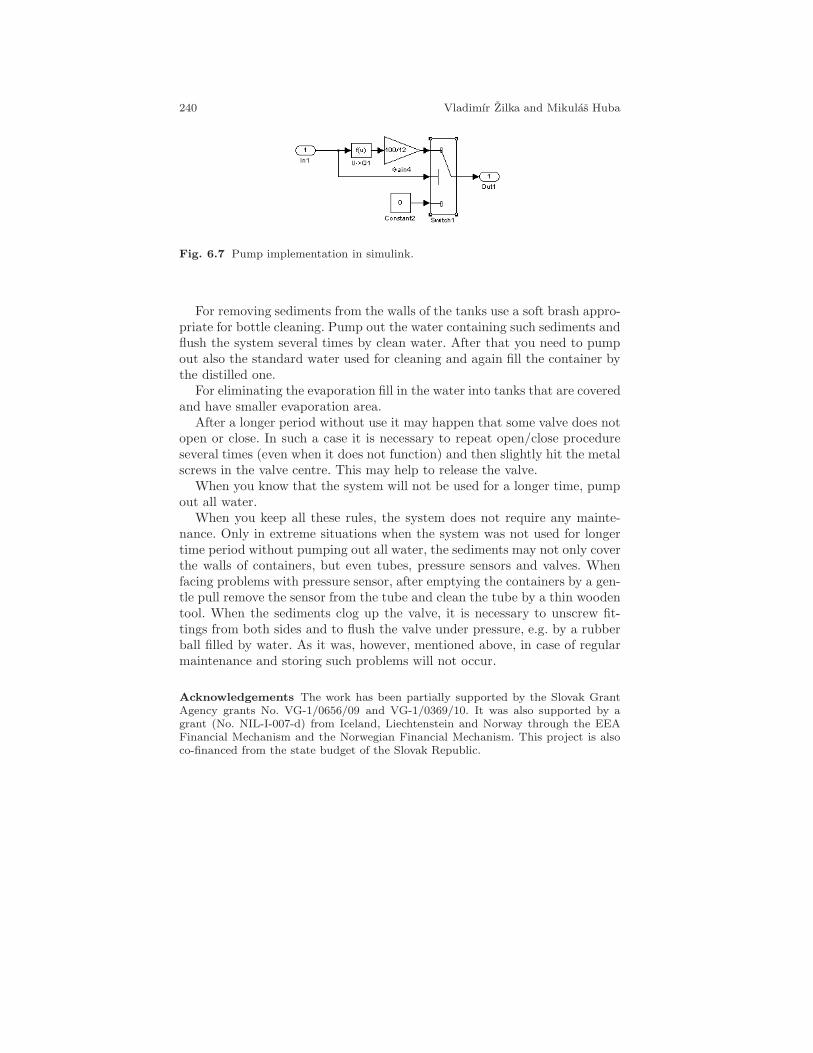
240 Vladimır Zilka and Mikulas Huba
Fig. 6.7 Pump implementation in simulink.
For removing sediments from the walls of the tanks use a soft brash appro-priate for bottle cleaning. Pump out the water containing such sediments andflush the system several times by clean water. After that you need to pumpout also the standard water used for cleaning and again fill the container bythe distilled one.
For eliminating the evaporation fill in the water into tanks that are coveredand have smaller evaporation area.
After a longer period without use it may happen that some valve does notopen or close. In such a case it is necessary to repeat open/close procedureseveral times (even when it does not function) and then slightly hit the metalscrews in the valve centre. This may help to release the valve.
When you know that the system will not be used for a longer time, pumpout all water.
When you keep all these rules, the system does not require any mainte-nance. Only in extreme situations when the system was not used for longertime period without pumping out all water, the sediments may not only coverthe walls of containers, but even tubes, pressure sensors and valves. Whenfacing problems with pressure sensor, after emptying the containers by a gen-tle pull remove the sensor from the tube and clean the tube by a thin woodentool. When the sediments clog up the valve, it is necessary to unscrew fit-tings from both sides and to flush the valve under pressure, e.g. by a rubberball filled by water. As it was, however, mentioned above, in case of regularmaintenance and storing such problems will not occur.
Acknowledgements The work has been partially supported by the Slovak GrantAgency grants No. VG-1/0656/09 and VG-1/0369/10. It was also supported by agrant (No. NIL-I-007-d) from Iceland, Liechtenstein and Norway through the EEAFinancial Mechanism and the Norwegian Financial Mechanism. This project is alsoco-financed from the state budget of the Slovak Republic.

6 Laboratory Model of Coupled Tanks 241
References
Zilka V (2007) Nonlinear controllers for a fluid tank system. Master’s thesis, Fac-ulty of Electrical Engineering and IT, Slovak University of Technology, Bratislava,Slovakia, (in Slovak)

242 Vladimır Zilka and Mikulas Huba
Comments – Remarks

6 Laboratory Model of Coupled Tanks 243
Comments – Remarks

244 Vladimır Zilka and Mikulas Huba
Comments – Remarks

6 Laboratory Model of Coupled Tanks 245
Comments – Remarks

Chapter 7
Constrained PID ControlTasks for Coupled Tanks Control
Vladimır Zilka and Mikulas Huba
Abstract This chapter treats basic issues of linear and non-linear controller’sdesign applied to control of hydraulic plant of availabe three-tank-system.Controllers based on approximation of the given non-linear system by thefirst order linear system by step responses are proposed and compared withcontrollers based on the analytical linearization of the nonlinear model in afixed operating point, by the input-output linearization in the actual state(exact linearization) and around a generalized operating point are developedand verified for the one-level and two-level system.
7.1 Introduction
A plant to be controlled may be modelled and identified in many ways. It ise.g. possible to derive mathematical models of the plant that for a given datashow nice matching but when used for the controller design, the resultingperformance will be pure. In case of inaccurate, or inappropriate mathemati-cal model, the resulting regulators would function only in simulations. That’swhy we will be dealing from now with the description of the real plant, estima-tion of its model, identification of its parameters as well as with confrontationof results achieved in control of the plant with the performance required inthe controller design.
In the next paragraph, we will show some examples of simple P, PI andPD controllers for different tanks’ configurations, from the simplest one tank
Vladimır ZilkaFaculty of Electrical Engineering and Information Technology, Slovak University ofTechnology in Bratislava, e-mail: [email protected]
Mikulas HubaFaculty of Electrical Engineering and Information Technology, Slovak University ofTechnology in Bratislava, e-mail: [email protected]
247
248 Vladimır Zilka and Mikulas Huba
system, with closed output valves, through one-level systems with one inflowand one outflow up to two-level system linearized by generalized input-outputlinearization and controlled by the PD2 controller.
7.2 Basic P and PI controllers
At the beginning, it would be the best to introduce the simplest case ofhydraulic system’s configuration. In doing so we will consider one-level systemwhich has all the valves closed. The pump feeding the liquid into this tankwill represent the actuator. Under control, such system behaves as simpleintegrator. Considering 6.1 we will define differential equations of such systemin the following form:
x1 =1
A1u1
y1 = x1 (7.1)
Obviously, we are dealing with linear system with the transfer function
F1(s) =Y1 (s)
U1 (s)=
1
A1s
i.e. with integrator having the integral time constant A1 (gain 1/A1). Fromtheory we know that to stabilize such a system (7.1), P-controller with a gainP1 would be sufficient. The closed loop transfer function will be:
G(s) =P1F1(s)
1 + P1F1(s)=
P1
A1s+ P1
If we want to control this system, we can request it to behave as the firstorder linear system with the transfer function
G(s) =1
T1s+ 1
In such a case, the P-controller’s gain results as
P1 =A1
T1
It is clear that by choosing the time constant T1, we are able to definethe dynamics of the closed loop that might also be expressed by its closedloop pole α = −1/T1. By decreasing this time constant, when the closed looppole is being shifted to −∞, we can speed up the transients processes. Andcontrary, by increasing T1, when the pole is shifted towards the origin, we
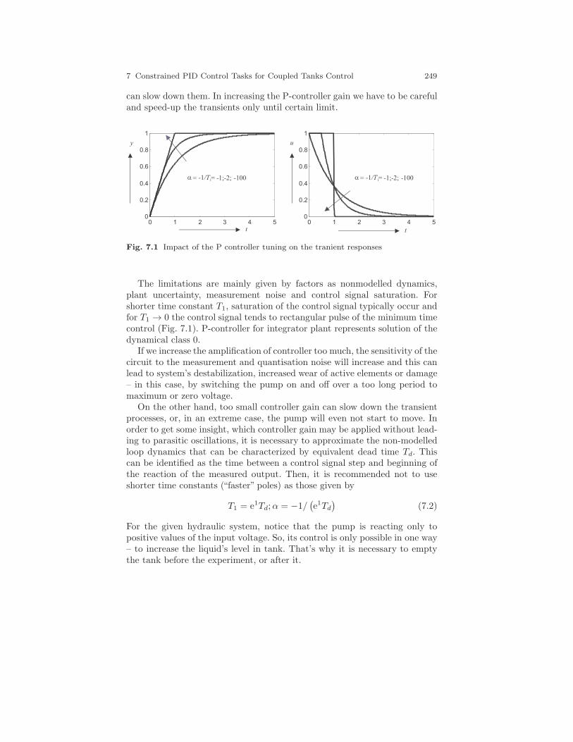
7 Constrained PID Control Tasks for Coupled Tanks Control 249
can slow down them. In increasing the P-controller gain we have to be carefuland speed-up the transients only until certain limit.
Fig. 7.1 Impact of the P controller tuning on the tranient responses
The limitations are mainly given by factors as nonmodelled dynamics,plant uncertainty, measurement noise and control signal saturation. Forshorter time constant T1, saturation of the control signal typically occur andfor T1 → 0 the control signal tends to rectangular pulse of the minimum timecontrol (Fig. 7.1). P-controller for integrator plant represents solution of thedynamical class 0.
If we increase the amplification of controller too much, the sensitivity of thecircuit to the measurement and quantisation noise will increase and this canlead to system’s destabilization, increased wear of active elements or damage– in this case, by switching the pump on and off over a too long period tomaximum or zero voltage.
On the other hand, too small controller gain can slow down the transientprocesses, or, in an extreme case, the pump will even not start to move. Inorder to get some insight, which controller gain may be applied without lead-ing to parasitic oscillations, it is necessary to approximate the non-modelledloop dynamics that can be characterized by equivalent dead time Td. Thiscan be identified as the time between a control signal step and beginning ofthe reaction of the measured output. Then, it is recommended not to useshorter time constants (“faster” poles) as those given by
T1 = e1Td;α = −1/(e1Td
)(7.2)
For the given hydraulic system, notice that the pump is reacting only topositive values of the input voltage. So, its control is only possible in one way– to increase the liquid’s level in tank. That’s why it is necessary to emptythe tank before the experiment, or after it.
250 Vladimır Zilka and Mikulas Huba
7.2.1 PI-controller
Now, let’s consider situation with opened outflow valve characterized with theflow coefficient c1. In this case the one-level system will be in the form 6.1.This system does no longer behave as pure integrator. Let’s try to controlit, at the beginning, with P-controller, designed in the previous part. Byexamining few operating point, we will realize that P-controller can’t controlthis system without the permanent control error. It is no surprise, if wetake into account that the opened outflow requires permanent inflow, butthe zero control error leads to zero inflow. With zero control error generatesthe P-controller zero action, but considering the fact that the liquid outflowsfrom the tank, it decreases the liquid’s level below the desired values. Tocompensate the outgoing liquid we have to use more advanced controllers.
The easiest way to compensate the outgoing water is to add parallel signalto the output of the controller. Such constant signal set usually manuallywas originally called as reset (offset). Later, this was replaced by automaticreset denoted today as the integral action and produced directly by the con-troller. By this modification we will obtain the PI-controller. The goal ofthe integral action is to integrate the control error values multiplicated bya suitable constant what will continuously increase the controller output –until the complete removal of the control error. The transfer function of suchPI-controller is:
R(s) = P +I
s
where P represents the gain of the proportional action of the controller andI is the gain of the integral action.
An easy experimental way to set up the PI-controller’s parameters maybe based on measured step-responses of the system. The step-responses ofthe system contain information about the basic dynamic attributes of thesystem and this is why it enables us to set up the controller’s parametersbetter than by the frequently used trial and error method. At the sametime, we have to realize that the step-response method was developed forthe responses of linear system to a unit step. Our system (6.1) is, however, anonlinear one. We can’t thus talk about the system’s step-responses for thewhole scope of liquid’s levels. The obtained information will depend on thechoice of concrete operating point, in which the step will be measured. Forthe PI-controller design having the best attributes in the most ample areas,it may seem to be useful to choose the operating point approximately in themiddle of the working area.
In the surroundings of chosen operating point we will approximate ournon-linear system (6.1) by the first order linear model. This will be obtainedby the step-response method from step responses measured firstly by settingup by appropriate input pump voltage the liquid’s level approximatelly to thethe middle of the tank hight and here to stabilize it for some time, optimallyfew centimeters under the middle. When the liquid’s level will be stabilized,
7 Constrained PID Control Tasks for Coupled Tanks Control 251
we will switch the pump input to higher voltage by approximately 1V stepand wait again for the liquid’s level to stabilize (it should stabilize few cen-timeters over the middle). From the measured step-response we will find outby constructing tangent at the origin the approximate value of time constantT1n and the value of the approximative plant gain K1 = ∆y/∆u.
So, in a close surroundings of the operating point corresponding to theinput voltage about u1 = 4V the system may be approximated by lineartransfer function
F1(s) =K1
T1ns+ 1
Then, in the previous paragraph mentioned P-controller design may nowbe used as well. When the open loop transfer function was in the case of the P-controller design given as 1/T1s the closed loop had the transfer 1/ (T1s+ 1).Now, we will design controller to yield the same open loop transfer functionas previously, i.e. 1/T1s, what yields
R1(s) =1
T1s· 1
F1(s)=
T1ns+ 1
K1T1s=
T1n
K1T1+
1
K1T1s
Thus the P and I actions will be
P1 =T1n
K1T1
I1 =1
K1T1
After calculating and testing this tuning we recommend you to experimenta bit and to track the influence of the changes of P1 and I1 on the controlperformance. You may observe that the achieved dynamics is differnt from theone possible pulse at saturation that was typical for the P controller design.This soultion represents basic part of the PI controller of the dynamical class0 (it should yet be completed by a prefilter with the time constant T1n – thenthe control signal after a setpoint step exponentially increases monotonicallyto its new steady-state value). Attempts to achieve faster dynamics may beconnected with strong overshooting of the output signal.
7.2.2 PI1 controller
Improved dynamics for larger setpoint steps without producing windup effectis possible to achieve by the so called PI1 controller that typically has oneinterval of the control signal at the saturation limit. This controller is based onreconstruction of the equivalent input or output disturbances by appropriateobserver using inverse or parallel plant model. Since the hydraulic plant (6.1)
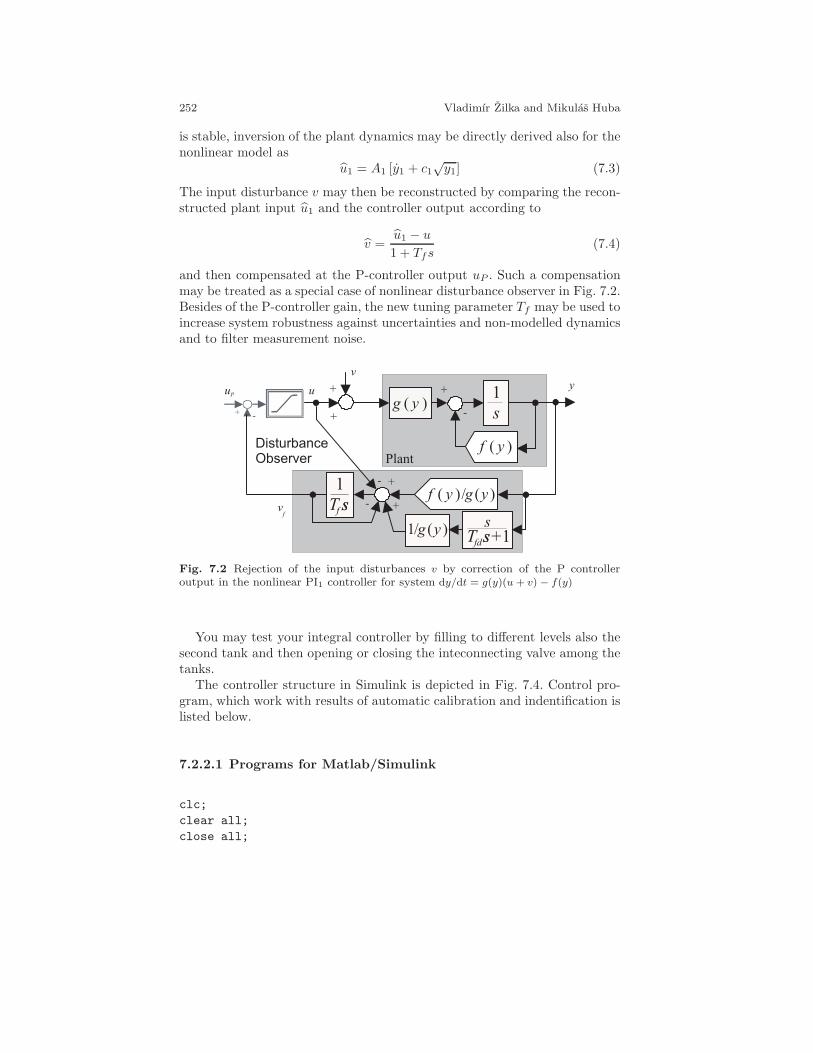
252 Vladimır Zilka and Mikulas Huba
is stable, inversion of the plant dynamics may be directly derived also for thenonlinear model as
u1 = A1 [y1 + c1√y1] (7.3)
The input disturbance v may then be reconstructed by comparing the recon-structed plant input u1 and the controller output according to
v =u1 − u
1 + Tfs(7.4)
and then compensated at the P-controller output uP . Such a compensationmay be treated as a special case of nonlinear disturbance observer in Fig. 7.2.Besides of the P-controller gain, the new tuning parameter Tf may be used toincrease system robustness against uncertainties and non-modelled dynamicsand to filter measurement noise.
Fig. 7.2 Rejection of the input disturbances v by correction of the P controlleroutput in the nonlinear PI1 controller for system dy/dt = g(y)(u + v) − f(y)
You may test your integral controller by filling to different levels also thesecond tank and then opening or closing the inteconnecting valve among thetanks.
The controller structure in Simulink is depicted in Fig. 7.4. Control pro-gram, which work with results of automatic calibration and indentification islisted below.
7.2.2.1 Programs for Matlab/Simulink
clc;
clear all;
close all;
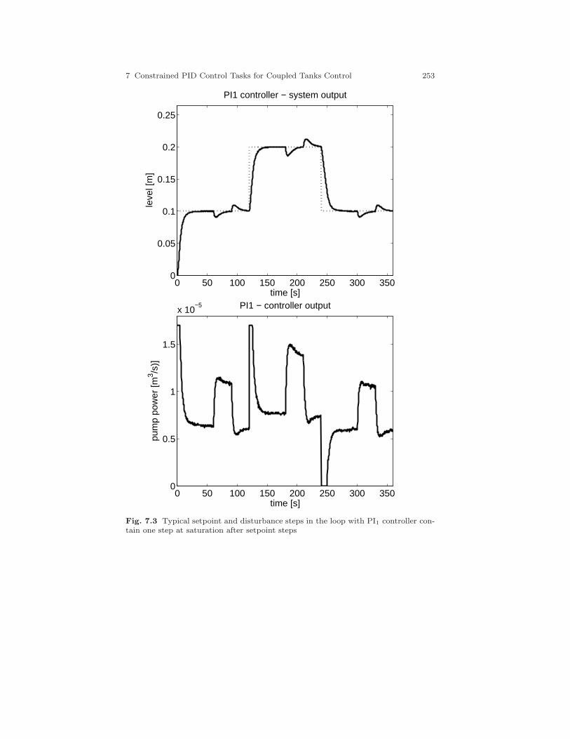
7 Constrained PID Control Tasks for Coupled Tanks Control 253
0 50 100 150 200 250 300 3500
0.05
0.1
0.15
0.2
0.25
time [s]
leve
l [m
]
PI1 controller − system output
0 50 100 150 200 250 300 3500
0.5
1
1.5
x 10−5
time [s]
pum
p po
wer
[m3 /s
)]
PI1 − controller output
Fig. 7.3 Typical setpoint and disturbance steps in the loop with PI1 controller con-tain one step at saturation after setpoint steps
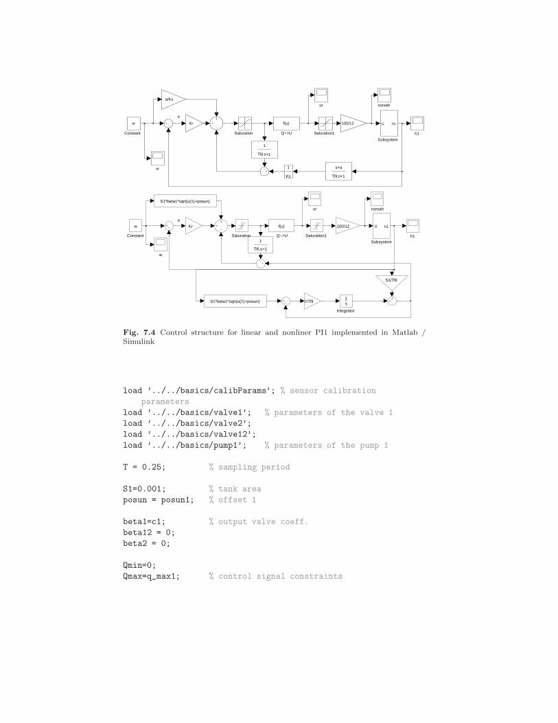
254 Vladimır Zilka and Mikulas Huba
e
w
ur rozsah
h1
s+a
Tfil.s+1
1
Ks
1
Tfil.s+1
Subsystem
U h1
Saturation1Saturation Q−>U
f(u) 100/12Kr
a/Ks
Constant
w
e
w
ur rozsah
h11
Tfil.s+1
Subsystem
U h1
Saturation1Saturation
S1*beta1*sqrt(u(1)+posun)
S1*beta1*sqrt(u(1)+posun)
Q−>U
f(u)
Integrator
1s
S1/Tfil
1/Tfil
100/12Kr
Constant
w
Fig. 7.4 Control structure for linear and nonliner PI1 implemented in Matlab /Simulink
load ’../../basics/calibParams’; % sensor calibration
parameters
load ’../../basics/valve1’; % parameters of the valve 1
load ’../../basics/valve2’;
load ’../../basics/valve12’;
load ’../../basics/pump1’; % parameters of the pump 1
T = 0.25; % sampling period
S1=0.001; % tank area
posun = posun1; % offset 1
beta1=c1; % output valve coeff.
beta12 = 0;
beta2 = 0;
Qmin=0;
Qmax=q_max1; % control signal constraints
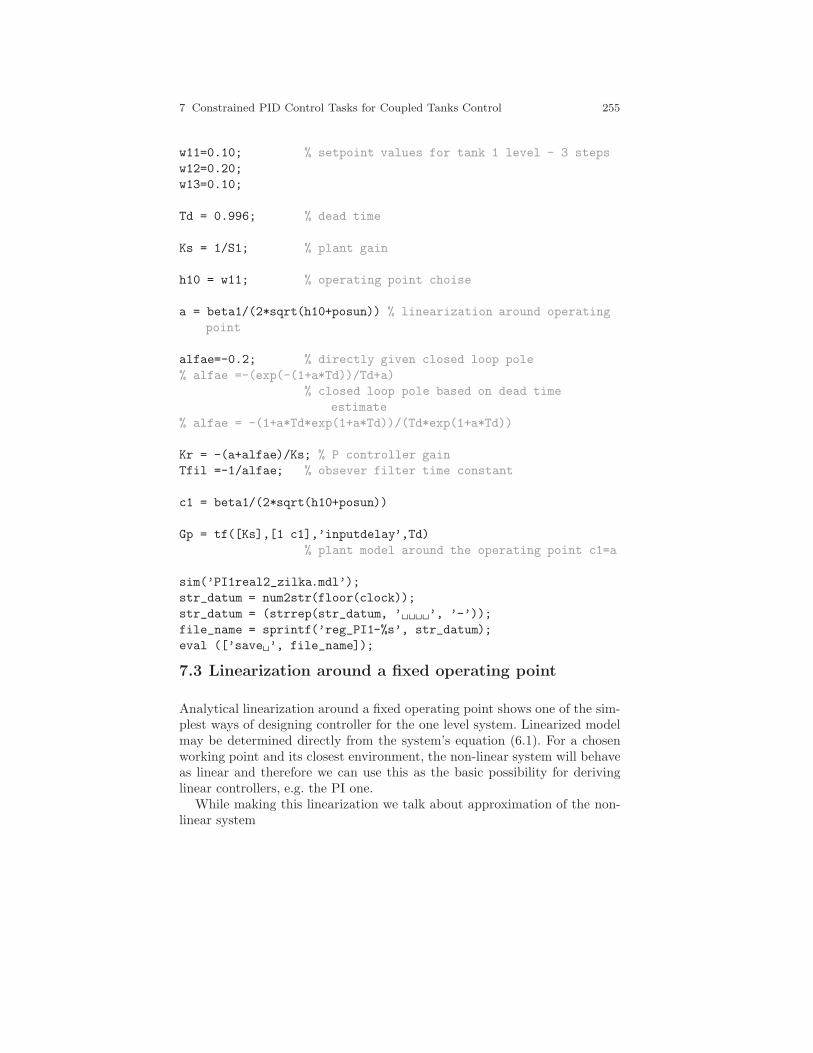
7 Constrained PID Control Tasks for Coupled Tanks Control 255
w11=0.10; % setpoint values for tank 1 level - 3 steps
w12=0.20;
w13=0.10;
Td = 0.996; % dead time
Ks = 1/S1; % plant gain
h10 = w11; % operating point choise
a = beta1/(2*sqrt(h10+posun)) % linearization around operating
point
alfae=-0.2; % directly given closed loop pole
% alfae =-(exp(-(1+a*Td))/Td+a)
% closed loop pole based on dead time
estimate
% alfae = -(1+a*Td*exp(1+a*Td))/(Td*exp(1+a*Td))
Kr = -(a+alfae)/Ks; % P controller gain
Tfil =-1/alfae; % obsever filter time constant
c1 = beta1/(2*sqrt(h10+posun))
Gp = tf([Ks],[1 c1],’inputdelay’,Td)
% plant model around the operating point c1=a
sim(’PI1real2_zilka.mdl’);
str_datum = num2str(floor(clock));
str_datum = (strrep(str_datum, ’ ’, ’-’));
file_name = sprintf(’reg_PI1-%s’, str_datum);
eval ([’save ’, file_name]);
7.3 Linearization around a fixed operating point
Analytical linearization around a fixed operating point shows one of the sim-plest ways of designing controller for the one level system. Linearized modelmay be determined directly from the system’s equation (6.1). For a chosenworking point and its closest environment, the non-linear system will behaveas linear and therefore we can use this as the basic possibility for derivinglinear controllers, e.g. the PI one.
While making this linearization we talk about approximation of the non-linear system
256 Vladimır Zilka and Mikulas Huba
x1 = f(x1, u1)
y1 = g(x1)
by a linear system
∆x1 = A∆x1 +B∆u1
∆y = C∆x1
where ∆x1 = x1 − x10 , ∆u1 = u1 − u10 , ∆y1 = y1 − y10 and x10 , u10 , y10 isour fixed operating point. It is to stress that the linearization is consideredaround a steady state, state, input and output are replaced by deviationsfrom it as: ∆x1, ∆u1 and ∆y1 and the matrices A, B and C are in generalgiven as:
A =
(∂f
∂x1
)
x1=x10,u1=u10
,B =
(∂f
∂u1
)
x1=x10,u1=u10
,C =
(∂g
∂x1
)
x1=x10,u1=u10
In case on one level hydraulic system (6.1)we get by such a linearization
∆x1 =1
A1∆u1 −
c12√x10
∆x1
∆y1 = ∆x1 (7.5)
We would like to point that (7.5) is not valid for x10 = 0. Taking into accountthat our system (7.5) is linear, we can consider its velocity transfer function
F1(s) =∆Y1(s)
∆U1(s)=
1A1
s+ c12√x10
Now for this system we propose PI-controller (for the first order linear sys-tem). Transfer function of the controller should again be made in such away to yield an open transfer function 1/T1s what may e.g. be achieved bychoosing
R1(s) =1
T1s· 1
F1(s)=
s+ c12√x10
1AT1s
=A1
T1+
A1c12T1
√x10s
where
P1 =A1
T1
I1 =A1c1
2T1√x10
are gains of P1 a I1 action of the controller. Note that the time constantT1 can be easily obtained from step-response of the system. We should not
7 Constrained PID Control Tasks for Coupled Tanks Control 257
omit the fact, that by designing the controller, we proceed from the system(7.5), which works with deviations from steady state, not with the absolutevaraibles. That’s why the controller is using them as well, i.e. it holds
R1(s) =∆U1(s)
∆E1(s)
where ∆U1(s) and ∆E1(s) are Laplace transforms of the deviations of thecontroller output, ∆u1 = u1 − u10 and of the control error, ∆e1 = e1 − e10 ,from steady states u10 a e10 . Of course, for control error in steady state ise10 = 0. In this case ∆e1 = e1, but at the controller output one still hasto consider deviation signal ∆u1. The system (6.1), which we are in factcontrolling, has as its input directly u. So, we need to arrange the controlleroutput by adding the stabilized steady-state value u10 and thus obtainingdirectly u1
u1 = ∆u1 + u10
The value u10 represents the stabilized value of the pump’s voltage, at whichthe liquid’s level or liquid’s volume in the tank has the stabilized value x10 .The numerical value u10 is, off course, needed at the implementation of thecontroller. We’ll define it based on system’s (6.1). In a steady-state all timederivatives are zero, thus x1 = 0. After substituting into (6.1) we’ll obtainu10 defined as
u10 = A1c1√x10
7.4 Exact Feedback Linearization
In this task, we would like to control the liquid’s level for different operatingpoints. By appropriate gain scheduling it is possible to have various operatingpoints and the associated controllers and then to switch between them, butas more practical it seems to schedule the controller parameters continuously.This is usually done by the input-output feedback linearization. In general,it is supposed a non-linear system in the following form:
x = f(x, u)
y = g(x)
where the state x ∈ Rn, the input u ∈ Rm, the output y ∈ Rp. Find, ifpossible, a static state feedback
u = ϕ(v, x)
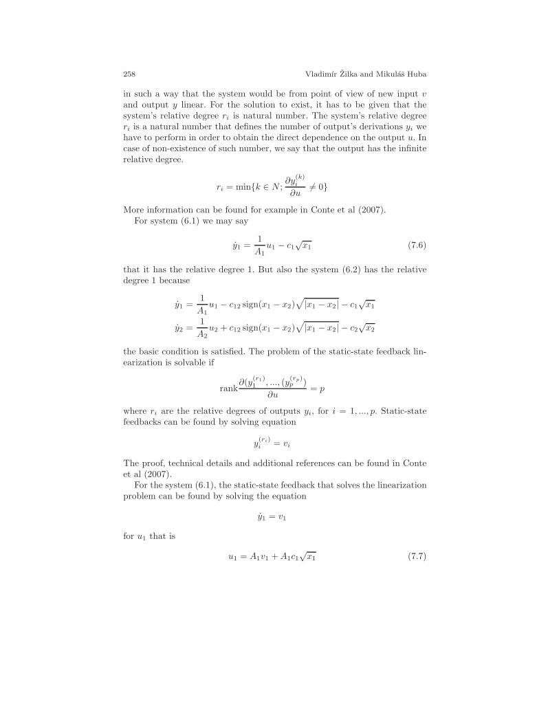
258 Vladimır Zilka and Mikulas Huba
in such a way that the system would be from point of view of new input vand output y linear. For the solution to exist, it has to be given that thesystem’s relative degree ri is natural number. The system’s relative degreeri is a natural number that defines the number of output’s derivations yi wehave to perform in order to obtain the direct dependence on the output u. Incase of non-existence of such number, we say that the output has the infiniterelative degree.
ri = mink ∈ N ;∂y
(k)i
∂u6= 0
More information can be found for example in Conte et al (2007).For system (6.1) we may say
y1 =1
A1u1 − c1
√x1 (7.6)
that it has the relative degree 1. But also the system (6.2) has the relativedegree 1 because
y1 =1
A1u1 − c12 sign(x1 − x2)
√|x1 − x2| − c1
√x1
y2 =1
A2u2 + c12 sign(x1 − x2)
√|x1 − x2| − c2
√x2
the basic condition is satisfied. The problem of the static-state feedback lin-earization is solvable if
rank∂(y
(r1)1 , ..., (y
(rp)p )
∂u= p
where ri are the relative degrees of outputs yi, for i = 1, ..., p. Static-statefeedbacks can be found by solving equation
y(ri)i = vi
The proof, technical details and additional references can be found in Conteet al (2007).
For the system (6.1), the static-state feedback that solves the linearizationproblem can be found by solving the equation
y1 = v1
for u1 that is
u1 = A1v1 +A1c1√x1 (7.7)

7 Constrained PID Control Tasks for Coupled Tanks Control 259
When we apply this, the feedback we get from the original system (6.1) linearsystem y1 = v1 with transfer function:
F1(s) =1
s
Now it is enough to design controller which will provide the required loopbehavior. It will be necessary for it to have opened loop transfer function1
T1s. When we talk about simple first degree integrator, in this case it is
enough use simple P-controller. Its gain will be
P1 =1
T1
For the two-level system (6.2) we will do the same. By requiring
y1 = v1
y2 = v2
the solution will be given equations for u1 and u2
u1 = A1v1 +A1c12 sign(x1 − x2)√
|x1 − x2|+A1c1√x1
u2 = A2v2 −A2c12 sign(x1 − x2)√|x1 − x2|+A2c2
√x2
Similarly to previous case, after application of these feedbacks we obtaintwo independent (decoupled) systems y1 = v1, y2 = v2 having the transferfunctions
F1(s) =1
s
F2(s) =1
s
We can continue again in the same way as with the one level system. As wenow have two independent liear systems, for each level we can design separateP-controller.
P1 =1
T1
P2 =1
T2
We would like to recall as well the special case of two tanks connection. Itdiffers from (6.1) in the way that the outflow from the first tank is at zero –valve 1 is closed, the second pump is turned off and the liquid’s height in thesecond tank is controller by controlling the inflow into the first tank. We canwrite down the system equations as it follows:
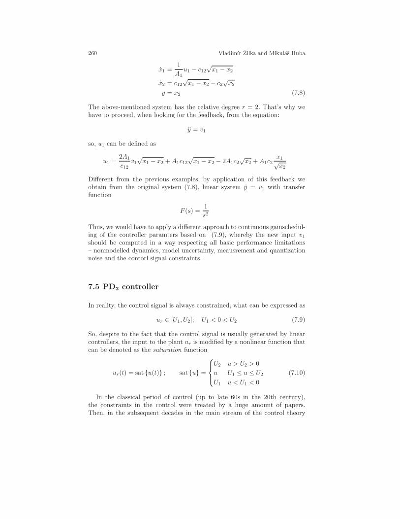
260 Vladimır Zilka and Mikulas Huba
x1 =1
A1u1 − c12
√x1 − x2
x2 = c12√x1 − x2 − c2
√x2
y = x2 (7.8)
The above-mentioned system has the relative degree r = 2. That’s why wehave to proceed, when looking for the feedback, from the equation:
y = v1
so, u1 can be defined as
u1 =2A1
c12v1√x1 − x2 +A1c12
√x1 − x2 − 2A1c2
√x2 +A1c2
x1√x2
Different from the previous examples, by application of this feedback weobtain from the original system (7.8), linear system y = v1 with transferfunction
F (s) =1
s2
Thus, we would have to apply a different approach to continuous gainschedul-ing of the controller paramters based on (7.9), whereby the new input v1should be computed in a way respecting all basic performance limitations– nonmodelled dynamics, model uncertainty, meausrement and quantizationnoise and the contorl signal constraints.
7.5 PD2 controller
In reality, the control signal is always constrained, what can be expressed as
ur ∈ [U1, U2]; U1 < 0 < U2 (7.9)
So, despite to the fact that the control signal is usually generated by linearcontrollers, the input to the plant ur is modified by a nonlinear function thatcan be denoted as the saturation function
ur(t) = sat u(t) ; sat u =
U2 u > U2 > 0
u U1 ≤ u ≤ U2
U1 u < U1 < 0
(7.10)
In the classical period of control (up to late 60s in the 20th century),the constraints in the control were treated by a huge amount of papers.Then, in the subsequent decades in the main stream of the control theory
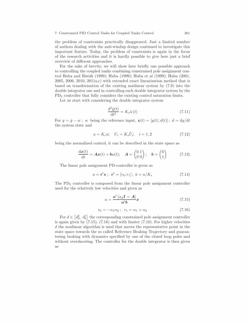
7 Constrained PID Control Tasks for Coupled Tanks Control 261
the problem of constraints practically disappeared. Just a limited numberof authors dealing with the anti-windup design continued to investigate thisimportant feature. Today, the problem of constraints is again in the focusof the research activities and it is hardly possible to give here just a briefoverview of different approaches.
For the sake of brevity, we will show here briefly one possible approachto controlling the coupled tanks combining constrained pole assignment con-trol Huba and Bistak (1999); Huba (1999); Huba et al (1999); Huba (2001,2005, 2006, 2010, 2011a,c) with extended exact linearization method that isbased on transformation of the existing nonlinear system by (7.9) into thedouble integrator one and in controlling such double integrator system by thePD2 controller that fully considers the existing control saturation limits.
Let us start with considering the double integrator system
d2y(t)
dt2= Ksu (t) (7.11)
For y = y − w ; w being the reference input, x(t) = [y(t), d(t)] ; d = dy/dtthe system state and
u = Ksu; Ui = KsUi; i = 1, 2 (7.12)
being the normalized control, it can be described in the state space as
dx(t)
dt= Ax(t) + bu(t); A =
(0 10 0
); b =
(01
)(7.13)
The linear pole assignment PD-controller is given as
u = rtx ; rt = [r0; r1] ; u = u/Ks (7.14)
The PD2 controller is composed from the linear pole assignment controllerused for the relatively low velocities and given as
u =at [α2I − A]
atbx (7.15)
r0 = −α1α2 ; r1 = α1 + α2 (7.16)
For d ∈[d20, d
10
]the corresponding constrained pole assignment controller
is again given by (7.15), (7.16) and with limiter (7.10). For higher velocitiesd the nonlinear algorithm is used that moves the representative point in thestate space towards the so called Reference Braking Trajectory and guaran-teeing braking with dynamics specified by one of the closed loop poles andwithout overshooting. The controller for the double integrator is then givenas
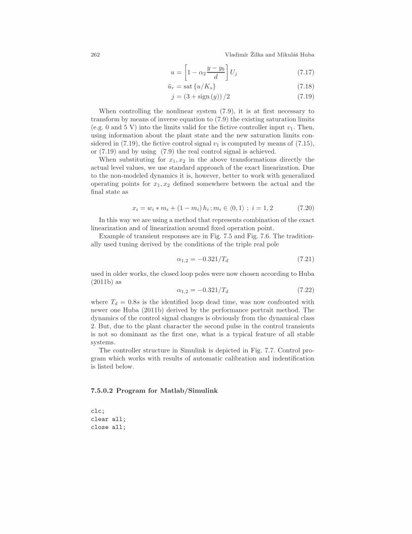
262 Vladimır Zilka and Mikulas Huba
u =
[1− α2
y − ybd
]Uj (7.17)
ur = sat u/Ks (7.18)
j = (3 + sign (y)) /2 (7.19)
When controlling the nonlinear system (7.9), it is at first necessary totransform by means of inverse equation to (7.9) the existing saturation limits(e.g. 0 and 5 V) into the limits valid for the fictive controller input v1. Then,using information about the plant state and the new saturation limits con-sidered in (7.19), the fictive control signal v1 is computed by means of (7.15),or (7.19) and by using (7.9) the real control signal is achieved.
When substituting for x1, x2 in the above transformations directly theactual level values, we use standard approach of the exact linearization. Dueto the non-modeled dynamics it is, however, better to work with generalizedoperating points for x1, x2 defined somewhere between the actual and thefinal state as
xi = wi ∗mi + (1−mi)hi ;mi ∈ 〈0, 1〉 ; i = 1, 2 (7.20)
In this way we are using a method that represents combination of the exactlinearization and of linearization around fixed operation point.
Example of transient responses are in Fig. 7.5 and Fig. 7.6. The tradition-ally used tuning derived by the conditions of the triple real pole
α1,2 = −0.321/Td (7.21)
used in older works, the closed loop poles were now chosen according to Huba(2011b) as
α1,2 = −0.321/Td (7.22)
where Td = 0.8s is the identified loop dead time, was now confronted withnewer one Huba (2011b) derived by the performance portrait method. Thedynamics of the control signal changes is obviously from the dynamical class2. But, due to the plant character the second pulse in the control transientsis not so dominant as the first one, what is a typical feature of all stablesystems.
The controller structure in Simulink is depicted in Fig. 7.7. Control pro-gram which works with results of automatic calibration and indentificationis listed below.
7.5.0.2 Program for Matlab/Simulink
clc;
clear all;
close all;
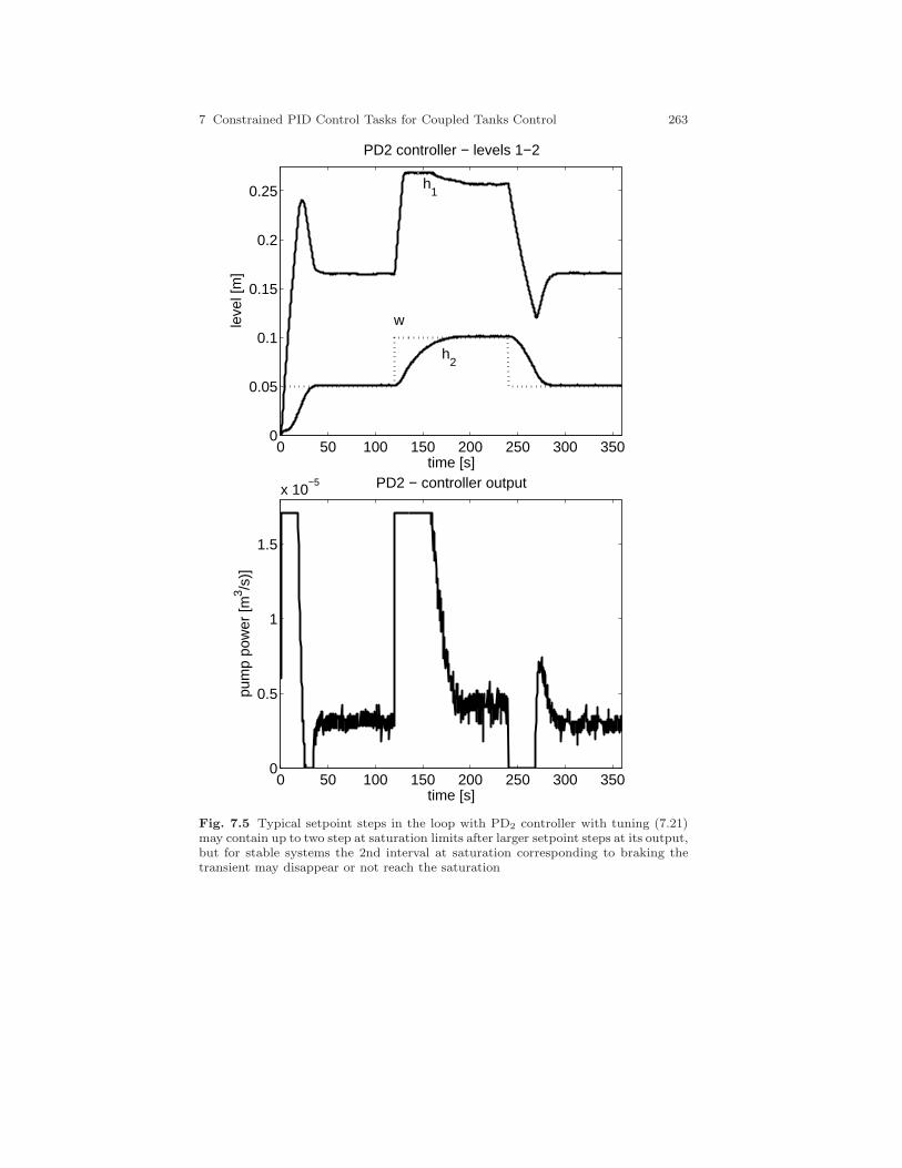
7 Constrained PID Control Tasks for Coupled Tanks Control 263
0 50 100 150 200 250 300 3500
0.05
0.1
0.15
0.2
0.25
time [s]
leve
l [m
]
PD2 controller − levels 1−2
h1
h2
w
0 50 100 150 200 250 300 3500
0.5
1
1.5
x 10−5
time [s]
pum
p po
wer
[m3 /s
)]
PD2 − controller output
Fig. 7.5 Typical setpoint steps in the loop with PD2 controller with tuning (7.21)may contain up to two step at saturation limits after larger setpoint steps at its output,but for stable systems the 2nd interval at saturation corresponding to braking thetransient may disappear or not reach the saturation
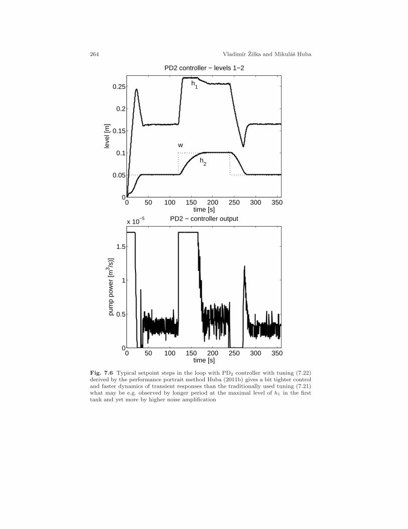
264 Vladimır Zilka and Mikulas Huba
0 50 100 150 200 250 300 3500
0.05
0.1
0.15
0.2
0.25
time [s]
leve
l [m
]
PD2 controller − levels 1−2
h1
h2
w
0 50 100 150 200 250 300 3500
0.5
1
1.5
x 10−5
time [s]
pum
p po
wer
[m3 /s
)]
PD2 − controller output
Fig. 7.6 Typical setpoint steps in the loop with PD2 controller with tuning (7.22)derived by the performance portrait method Huba (2011b) gives a bit tighter controland faster dynamics of transient responses than the traditionally used tuning (7.21)what may be e.g. observed by longer period at the maximal level of h1 in the firsttank and yet more by higher noise amplification
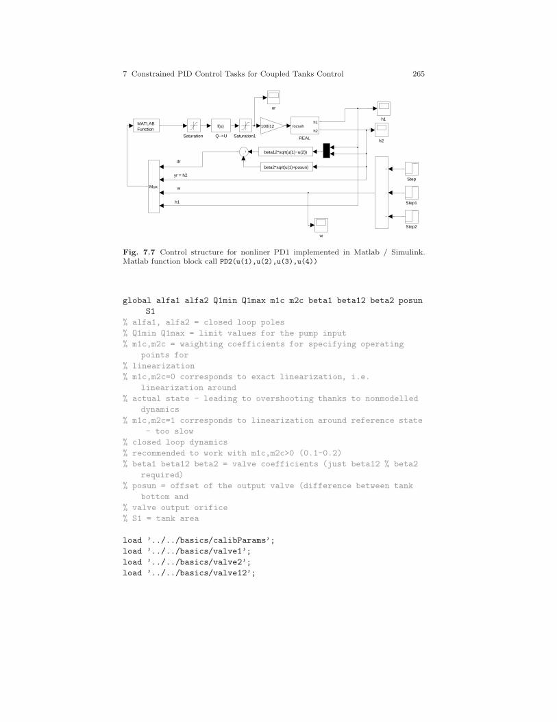
7 Constrained PID Control Tasks for Coupled Tanks Control 265
dr
yr = h2
w
h1
w
ur
h2
h1
Step2
Step1
Step
Saturation1Saturation REAL
rozsahh1
h2
beta2*sqrt(u(1)+posun)
beta12*sqrt(u(1)−u(2))
Q−>U
f(u)
Mux
MATLABFunction
100/12
Fig. 7.7 Control structure for nonliner PD1 implemented in Matlab / Simulink.Matlab function block call PD2(u(1),u(2),u(3),u(4))
global alfa1 alfa2 Q1min Q1max m1c m2c beta1 beta12 beta2 posun
S1
% alfa1, alfa2 = closed loop poles
% Q1min Q1max = limit values for the pump input
% m1c,m2c = waighting coefficients for specifying operating
points for
% linearization
% m1c,m2c=0 corresponds to exact linearization, i.e.
linearization around
% actual state - leading to overshooting thanks to nonmodelled
dynamics
% m1c,m2c=1 corresponds to linearization around reference state
- too slow
% closed loop dynamics
% recommended to work with m1c,m2c>0 (0.1-0.2)
% beta1 beta12 beta2 = valve coefficients (just beta12 % beta2
required)
% posun = offset of the output valve (difference between tank
bottom and
% valve output orifice
% S1 = tank area
load ’../../basics/calibParams’;
load ’../../basics/valve1’;
load ’../../basics/valve2’;
load ’../../basics/valve12’;
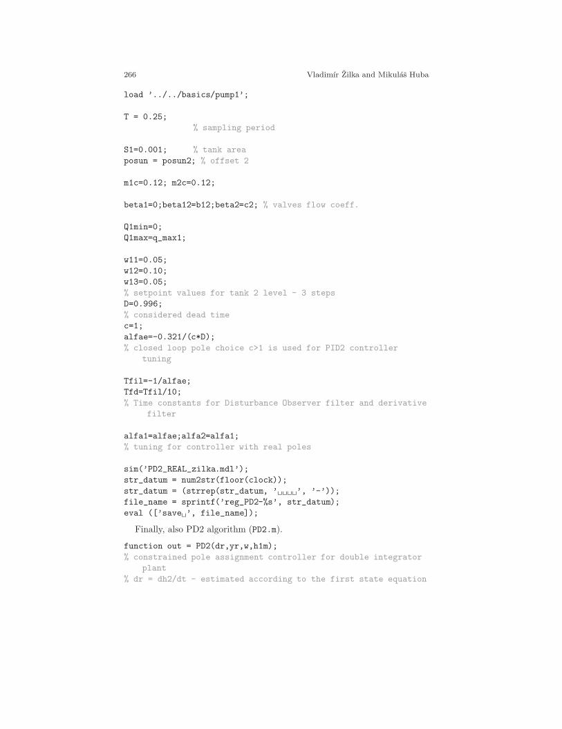
266 Vladimır Zilka and Mikulas Huba
load ’../../basics/pump1’;
T = 0.25;
% sampling period
S1=0.001; % tank area
posun = posun2; % offset 2
m1c=0.12; m2c=0.12;
beta1=0;beta12=b12;beta2=c2; % valves flow coeff.
Q1min=0;
Q1max=q_max1;
w11=0.05;
w12=0.10;
w13=0.05;
% setpoint values for tank 2 level - 3 steps
D=0.996;
% considered dead time
c=1;
alfae=-0.321/(c*D);
% closed loop pole choice c>1 is used for PID2 controller
tuning
Tfil=-1/alfae;
Tfd=Tfil/10;
% Time constants for Disturbance Observer filter and derivative
filter
alfa1=alfae;alfa2=alfa1;
% tuning for controller with real poles
sim(’PD2_REAL_zilka.mdl’);
str_datum = num2str(floor(clock));
str_datum = (strrep(str_datum, ’ ’, ’-’));
file_name = sprintf(’reg_PD2-%s’, str_datum);
eval ([’save ’, file_name]);
Finally, also PD2 algorithm (PD2.m).
function out = PD2(dr,yr,w,h1m);
% constrained pole assignment controller for double integrator
plant
% dr = dh2/dt - estimated according to the first state equation

7 Constrained PID Control Tasks for Coupled Tanks Control 267
% yr = h2 - measured level in tank 2
% w = reference value for tank 2
% h1m=h1 - measured level in tank 1
global alfa1 alfa2 Q1min Q1max m1c m2c beta1 beta12 beta2 posun
S1
% alfa1, alfa2 = closed loop poles
% Q1min Q1max = limit values for the pump input
% beta1 beta12 beta2 = valve coefficients (just beta1 % beta12
required)
% posun = offset of the output valve (difference between tank
bottom and
% valve output orifice
% ************signals transformations*************
h2m=yr; y = yr-w;
%s hifting reference state to the origin
w1 = ((beta2/beta12)^2)*(w+posun)+w;
% steady state level in tank 1
% corresponding to setpoint reference level w in tank 2
% posun = valve orifice offset
h1=m1c*w1+(1-m1c)*h1m;
h2=m2c*w+(1-m2c)*h2m;
% h1,h2 =operating points for linearization of tank 1 and 2
% m1c,m2c = waighting coefficients for specifying
% operating points for linearization
% m1c,m2c=0 correspond to exact linearization,
% i.e. linearization around actual state - leading
% to overshooting thanks to nonmodelled dynamics
% m1c,m2c=0 correspond to linearization around reference state
-
% too slow closed loop dynamics
% recommended to work with m1c,m2c>0 (0.1-0.2)
h12=abs(h1-h2);
z=sign(h1-h2);
a = beta12/(2*S1*sqrt(h12));
b = -(-beta12^2-1/2*(-2*beta2*h2-beta2*posun+beta2*h1)*beta12
/((h1-h2)^(1/2)*(h2+posun)^(1/2))+1/2*beta2^2);
% transformation to the normal form for output y=h2
% real control ur of pump with constraints Q1min, Q1max
% replaced by fictive input of a double integrator
% with limits Q12 and Q11
268 Vladimır Zilka and Mikulas Huba
Q12 = a*Q1max-b;
Q11 = a*Q1min-b;
% limit values of fictive input signal of double integrator
**************control algorithm*************
% control algorithm for constrained control
% of double integrators with real
% closed loop poles alfa1, alfa2
if (Q11*Q12>0)
if (h1m+h2m>w+w1)
u=Q1min;
else
u=Q1max;
end
ur=u;
else
if y>0
Q1j = Q12;
else
Q1j = Q11;
end
d1=Q11/alfa1;
d2=Q12/alfa1;
if(dr>d2) & (dr<d1)
u=(-alfa1*alfa2*y+(alfa1+alfa2)*dr);
% linear pole assignment
else
u=((1-alfa2*(y-0.5*(dr*dr/(Q1j)+Q1j/(alfa1*alfa1)))/dr)*
Q1j);
% nonlinear pole assignment
end
% constraining output
if (u>Q12)
u=Q12;
end
if (u<Q11)
u=Q11;
end
% ***********inverse transformation***********
% inverse transformation from the fictive
7 Constrained PID Control Tasks for Coupled Tanks Control 269
% double integrator input u to
% real input ur
ur = (u+b)/a;
end
out = ur;
7.6 Conclusion
We have described the basic possibilities of control of available hydraulic sys-tem established by different configuration of one or two containers with oneor two pumps. It is important to mention, that in case of control of real sys-tem with the mentioned controllers we will not obtain the ideally supposedresults. Certainly, due to modelling errors we will register some deviationsbetween supposed and real transients. The control performance will dependon the accuracy of identification and robustness of controller. As we will neverbe able to define the system’s parameters with 100% precision, the systemwild never behave as the perfect integrator and P-controller will not assurethe necessary quality of control. That’s why we propose to design the robustcontrollers having sufficient robustness against influence of disturbances, un-certainties and measurement noise. At the same time, these controllers shouldalso respect the available system’s limits. Such proposals for one-level systemcan be found for example Huba (2003); Pan et al (2005); Halas (2006); Almu-tairi and Zribi (2006); Zilka et al (2009). Further development of the above-mentioned procedures, as e.g. the disturbance decoupling problem of coupledtanks was studied in Zilka and Halas (2010) and non-interacting control ofcoupled tanks in Zilka and Halas (2011).
Acknowledgements The work has been partially supported by the Slovak GrantAgency grants No. VG-1/0656/09 and VG-1/0369/10. It was also supported by agrant (No. NIL-I-007-d) from Iceland, Liechtenstein and Norway through the EEAFinancial Mechanism and the Norwegian Financial Mechanism. This project is alsoco-financed from the state budget of the Slovak Republic.
References
Almutairi NB, Zribi M (2006) Sliding mode control of coupled tanks. Mechatronics16(7):427 – 441
Conte G, Moog C, Perdon A (2007) Algebraic Methods for Nonlinear Control Systems.Theory and Applications, 2nd edn. Communications and Control Engineering,Springer-Verlag, London
Halas M (2006) Quotients of noncommutative polynomials in nonlinear control sys-tems. In: 18th European Meeting on Cyberntetics and Systems Research, Vienna,Austria

270 Vladimır Zilka and Mikulas Huba
Huba M (1999) Dynamical classes in the minimum time pole assignment control. In:Computing Anticipatory Systems - CASYS ’98, Woodbury: American Institute ofPhysics, pp 499–512
Huba M (2001) Constrained control of the two tank system. In: 9th MediterraneanConference on Control and Automation, Dubrovnik, pp 93–98
Huba M (2003) Gain scheduled PI level control of a tank with variable cross section.In: 2nd IFAC Conference on Control Systems Design, Bratislava, Slovakia
Huba M (2005) P- und pd-polvorgaberegler fur regelstrecken mit begrenzter stell-grosse. Automatisierungstechnik AT 53(6):273–283
Huba M (2006) Constrained pole assignment control. In: Current Trends in NonlinearSystems and Control, L. Menini, L. Zaccarian, Ch. T. Abdallah, Edts., Birkhauser,Boston, pp 163–183
Huba M (2010) Designing robust controller tuning for dead time systems. In: IFACInt. Conf. System Structure and Control, Ancona, Italy
Huba M (2011a) Basic notions of robust constrained pid control. In: Selected topicson constrained and nonlinear control. M. Huba, S. Skogestad, M. Fikar, M. Hovd,T.A. Johansen, B. Roha¿-Ilkiv Editors, STU Bratislava - NTNU Trondheim
Huba M (2011b) Constrained pole assignment controller for sopdt plant. complexpoles. In: NIL Workshop on constrained and nonlinear control. M. Huba, S. Sko-gestad, M. Fikar, M. Hovd, T.A. Johansen, B. Roha¿-Ilkiv Editors, STU Bratislava- NTNU Trondheim
Huba M (2011c) Robust controller tuning for constrained double integrator. In: NILWorkshop on constrained and nonlinear control. M. Huba, S. Skogestad, M. Fikar,M. Hovd, T.A. Johansen, B. Roha¿-Ilkiv Editors, STU Bratislava - NTNU Trond-heim
Huba M, Bistak P (1999) Dynamic classes in the pid control. In: Proceedings of the1999 American Control Conference, San Diego: AACC
Huba M, Sovisova D, Oravec I (1999) Invariant sets based concept of the pole assign-ment control. In: European Control Conference ECC’99, Duesseldorf: VDI/VDE
Pan H, Wong H, Kapila V, de Queiroz MS (2005) Experimental validation of a non-linear backstepping liquid level controller for a state coupled two tank system.Control Engineering Practice 13(1):27 – 40
Zilka V, Halas M (2010) Disturbance decoupling of coupled tanks: From theory topractice. In: IFAC Symposium on System, Structure and Control - CSSS 2010,Ancona, Italy
Zilka V, Halas M (2011) Noninteracting control of coupled tanks: From theory topractice. In: 13th International Conference on Computer Aided Systems Theory -EUROCAST 2011, Las Palmas, Gran Canaria
Zilka V, Halas M, Huba M (2009) Nonlinear controllers for a fluid tank system.In: R. Moreno-Dıaz, F. Pichler, A. Quesada-Arencibia (Eds.): Computer AidedSystems Theory - EUROCAST 2009, Springer, Berlin, Germany, Lecture Notes inComputer Science, pp 618–625

7 Constrained PID Control Tasks for Coupled Tanks Control 271
Comments – Remarks

272 Vladimır Zilka and Mikulas Huba
Comments – Remarks

7 Constrained PID Control Tasks for Coupled Tanks Control 273
Comments – Remarks

274 Vladimır Zilka and Mikulas Huba
Comments – Remarks

Chapter 8
Remote Laboratory Software Module forThermo Optical Plant
Pavol Bistak
Abstract Virtual and remote laboratories play an important role in theeducation process of engineers. Their expansion is closely connected to thegrowth of Internet. This contribution describes how it is possible to install anduse the remote laboratory for the thermo optical plant. It explains the processof installation both the server and the client applications. Then the userinterface of the client application is discussed in details. An administrator ofthe remote laboratory can modify existing control structures therefore thereare special rules included in one section how to create new Simulink blockdiagrams in order to be compatible with the remote laboratory software.Thus one can set up the remote laboratory easily and it can be modified toher/his needs quickly.
8.1 Introduction
The remote laboratory software module for the uDAQ28/LT thermo opticalplant is represented by the client server application which main task is toenable remote experiments via Internet. Although the software has been de-signed to co-operate with the uDAQ28/LT real plant its usage is not limitedonly to this real system. The server part of the software is created by theprogram application written in the Java programming language. The serverapplication should be installed on the computer that directly controls thereal plant. The client part of the software is realized in the form of a Webpage with embedded Java applet. This provides a user friendly environmentto carry out remote experiments.
Pavol BistakInstitute of Control and Industrial Informatics, Slovak University of Technology inBratislava, e-mail: [email protected]
275
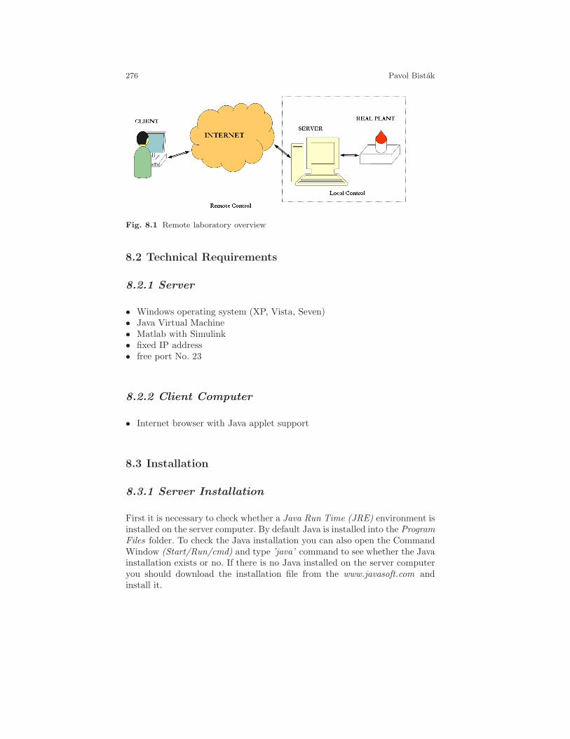
276 Pavol Bistak
Fig. 8.1 Remote laboratory overview
8.2 Technical Requirements
8.2.1 Server
• Windows operating system (XP, Vista, Seven)• Java Virtual Machine• Matlab with Simulink• fixed IP address• free port No. 23
8.2.2 Client Computer
• Internet browser with Java applet support
8.3 Installation
8.3.1 Server Installation
First it is necessary to check whether a Java Run Time (JRE) environment isinstalled on the server computer. By default Java is installed into the ProgramFiles folder. To check the Java installation you can also open the CommandWindow (Start/Run/cmd) and type ’java’ command to see whether the Javainstallation exists or no. If there is no Java installed on the server computeryou should download the installation file from the www.javasoft.com andinstall it.
8 Remote Laboratory Software Module for Thermo Optical Plant 277
The proper installation of the uDAQ28/LT thermo optical plant is anotherpreposition. The installation should be carried out according to the guide onthe installation CD. To check if the control of the real plant works locallyit is possible to run one of the predefined experiments from the installationCD.
In the case the above mentioned requirements are fulfilled the server ap-plication could be installed. Open the Server folder on the installation CDand double click the server install.bat file. During the process of installationthere will be a new folder called RemLabWorkspace created in the root di-rectory of the C: drive. Necessary Matlab files will be copied into this folder.Moreover the server application RemLabServer.exe will be copied into theRemLabWorkspace folder. Before running the server application it is recom-mended to check the setting of the serial port (in supplied block diagramsthat are placed in the directory C:\RemLabWorkspace).
Warning: Do not delete or move the folder C:\RemLabWorkspace. Thisfolder is fixed working directory of the server application. The RemLab-Server.exe application file can be moved from the C:\RemLabWorkspacefolder to any different place and it is also possible to create a shortcut placedat the desktop in order to run it quickly.
8.3.2 Client Installation
The client application is created in the form of a Java applet inserted into aWeb page. For the testing purposes the installation is not needed because itcan be run directly from the installation CD by clicking the client.html fileplaced in the Client\Application folder.
But the client application is aimed for a Web publication when it canbe accessible for all potential users. In this case it is necessary to upload thecontent of the Client\Application folder to the desired Web server. Then aftersetting the correct Internet address the client application is downloaded intothe Web browser window that enables running of Java applets.
8.4 Running the Client Server Application
The run of a client server application must be synchronized. First it isnecessary to run the server part of the application. After the server hasbeen successfully installed it is possible to run it by a double click to theRemLabServer.exe file that is (after the correct installation) placed in theC:\RemLabWorkspace folder. Depending on the server computer safety set-tings it can happen that the system will ask for confirmation of a trust tothe application.
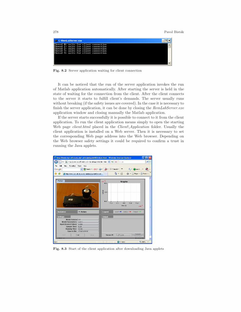
278 Pavol Bistak
Fig. 8.2 Server application waiting for client connection
It can be noticed that the run of the server application invokes the runof Matlab application automatically. After starting the server is held in thestate of waiting for the connection from the client. After the client connectsto the server it starts to fulfill client’s demands. The server usually runswithout breaking (if the safety issues are covered). In the case it is necessary tofinish the server application, it can be done by closing the RemLabServer.exeapplication window and closing manually the Matlab application.
If the server starts successfully it is possible to connect to it from the clientapplication. To run the client application means simply to open the startingWeb page client.html placed in the Client\Application folder. Usually theclient application is installed on a Web server. Then it is necessary to setthe corresponding Web page address into the Web browser. Depending onthe Web browser safety settings it could be required to confirm a trust inrunning the Java applets.
Fig. 8.3 Start of the client application after downloading Java applets
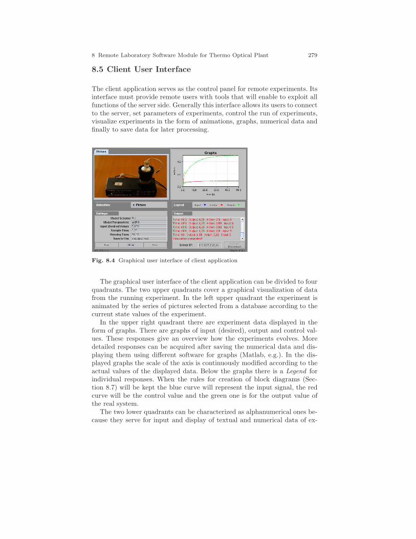
8 Remote Laboratory Software Module for Thermo Optical Plant 279
8.5 Client User Interface
The client application serves as the control panel for remote experiments. Itsinterface must provide remote users with tools that will enable to exploit allfunctions of the server side. Generally this interface allows its users to connectto the server, set parameters of experiments, control the run of experiments,visualize experiments in the form of animations, graphs, numerical data andfinally to save data for later processing.
Fig. 8.4 Graphical user interface of client application
The graphical user interface of the client application can be divided to fourquadrants. The two upper quadrants cover a graphical visualization of datafrom the running experiment. In the left upper quadrant the experiment isanimated by the series of pictures selected from a database according to thecurrent state values of the experiment.
In the upper right quadrant there are experiment data displayed in theform of graphs. There are graphs of input (desired), output and control val-ues. These responses give an overview how the experiments evolves. Moredetailed responses can be acquired after saving the numerical data and dis-playing them using different software for graphs (Matlab, e.g.). In the dis-played graphs the scale of the axis is continuously modified according to theactual values of the displayed data. Below the graphs there is a Legend forindividual responses. When the rules for creation of block diagrams (Sec-tion 8.7) will be kept the blue curve will represent the input signal, the redcurve will be the control value and the green one is for the output value ofthe real system.
The two lower quadrants can be characterized as alphanumerical ones be-cause they serve for input and display of textual and numerical data of ex-
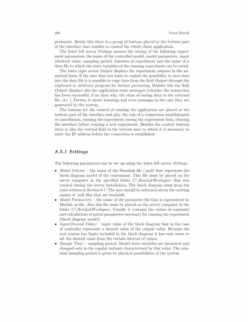
280 Pavol Bistak
periments. Beside this there is a group of buttons placed in the bottom partof the interface that enables to control the whole client application.
The lower left sector Settings assures the setting of the following experi-ment parameters: the name of the controlled model, model parameters, input(desired) value, sampling period, duration of experiment and the name of adata file to which the state variables of the running experiment can be saved.
The lower right sector Output displays the experiment outputs in the nu-merical form. If the user does not want to exploit the possibility to save datainto the data file it is possible to copy data from the field Output through theclipboard to arbitrary program for further processing. Besides this the fieldOutput displays also the application state messages (whether the connectionhas been successful, if no then why, the state of saving data to the externalfile, etc. ). Further it shows warnings and error messages in the case they aregenerated by the system.
The buttons for the control of running the application are placed at thebottom part of the interface and play the role of a connection establishmentor cancellation, running the experiment, saving the experiment data, clearingthe interface before running a new experiment. Besides the control buttonsthere is also the textual field in the bottom part to which it is necessary toenter the IP address before the connection is established.
8.5.1 Settings
The following parameters can be set up using the lower left sector Settings :
• Model Scheme – the name of the Simulink file (.mdl) that represents theblock diagram model of the experiment. This file must be placed on theserver computer in the specified folder C:\RemLabWorkspace that wascreated during the server installation. The block diagram must keep therules written in Section 8.7. The user should be informed about the existingnames of .mdl files that are available.
• Model Parameters – the name of the parameter file that is represented byMatlab .m file. Also this file must be placed on the server computer in thefolder C:\RemLabWorkspace. Usually it contains the values of constantsand calculations of initial parameters necessary for running the experiment(block diagram model).
• Input(Desired Value) – input value of the block diagram that in the caseof controller represents a desired value of the output value. Because thereal system has limits included in the block diagram it has only sense toset the desired value from the certain interval of values.
• Sample Time – sampling period. Model state variables are measured andchanged only in the regular instants characterized by this value. The min-imal sampling period is given by physical possibilities of the system.
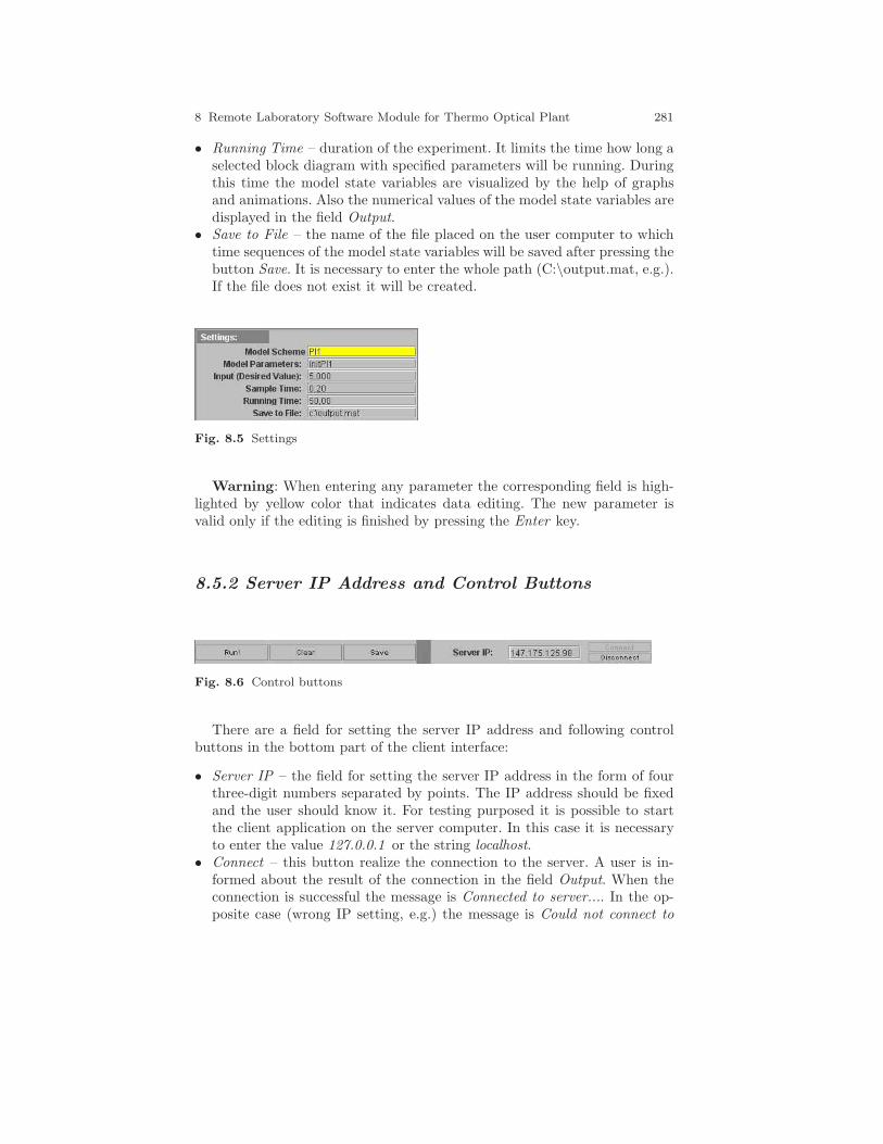
8 Remote Laboratory Software Module for Thermo Optical Plant 281
• Running Time – duration of the experiment. It limits the time how long aselected block diagram with specified parameters will be running. Duringthis time the model state variables are visualized by the help of graphsand animations. Also the numerical values of the model state variables aredisplayed in the field Output.
• Save to File – the name of the file placed on the user computer to whichtime sequences of the model state variables will be saved after pressing thebutton Save. It is necessary to enter the whole path (C:\output.mat, e.g.).If the file does not exist it will be created.
Fig. 8.5 Settings
Warning: When entering any parameter the corresponding field is high-lighted by yellow color that indicates data editing. The new parameter isvalid only if the editing is finished by pressing the Enter key.
8.5.2 Server IP Address and Control Buttons
Fig. 8.6 Control buttons
There are a field for setting the server IP address and following controlbuttons in the bottom part of the client interface:
• Server IP – the field for setting the server IP address in the form of fourthree-digit numbers separated by points. The IP address should be fixedand the user should know it. For testing purposed it is possible to startthe client application on the server computer. In this case it is necessaryto enter the value 127.0.0.1 or the string localhost.
• Connect – this button realize the connection to the server. A user is in-formed about the result of the connection in the field Output. When theconnection is successful the message is Connected to server.... In the op-posite case (wrong IP setting, e.g.) the message is Could not connect to
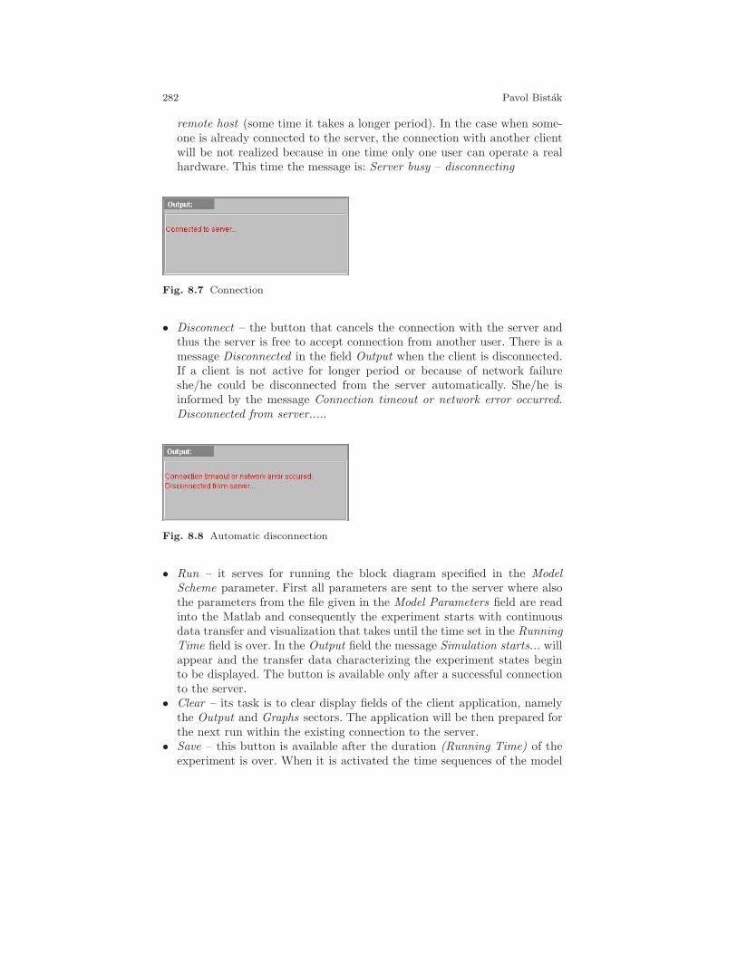
282 Pavol Bistak
remote host (some time it takes a longer period). In the case when some-one is already connected to the server, the connection with another clientwill be not realized because in one time only one user can operate a realhardware. This time the message is: Server busy – disconnecting
Fig. 8.7 Connection
• Disconnect – the button that cancels the connection with the server andthus the server is free to accept connection from another user. There is amessage Disconnected in the field Output when the client is disconnected.If a client is not active for longer period or because of network failureshe/he could be disconnected from the server automatically. She/he isinformed by the message Connection timeout or network error occurred.Disconnected from server.....
Fig. 8.8 Automatic disconnection
• Run – it serves for running the block diagram specified in the ModelScheme parameter. First all parameters are sent to the server where alsothe parameters from the file given in the Model Parameters field are readinto the Matlab and consequently the experiment starts with continuousdata transfer and visualization that takes until the time set in the RunningTime field is over. In the Output field the message Simulation starts... willappear and the transfer data characterizing the experiment states beginto be displayed. The button is available only after a successful connectionto the server.
• Clear – its task is to clear display fields of the client application, namelythe Output and Graphs sectors. The application will be then prepared forthe next run within the existing connection to the server.
• Save – this button is available after the duration (Running Time) of theexperiment is over. When it is activated the time sequences of the model
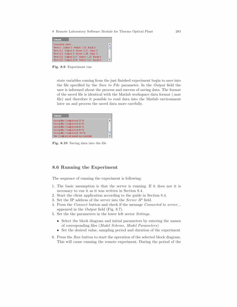
8 Remote Laboratory Software Module for Thermo Optical Plant 283
Fig. 8.9 Experiment run
state variables coming from the just finished experiment begin to save intothe file specified by the Save to File parameter. In the Output field theuser is informed about the process and success of saving data. The formatof the saved file is identical with the Matlab workspace data format (.matfile) and therefore it possible to read data into the Matlab environmentlater on and process the saved data more carefully.
Fig. 8.10 Saving data into the file
8.6 Running the Experiment
The sequence of running the experiment is following:
1. The basic assumption is that the server is running. If it does not it isnecessary to run it as it was written in Section 8.4.
2. Start the client application according to the guide in Section 8.4.3. Set the IP address of the server into the Server IP field.4. Press the Connect button and check if the message Connected to server...
appeared in the Output field (Fig. 8.7).5. Set the the parameters in the lower left sector Settings.
• Select the block diagram and initial parameters by entering the namesof corresponding files (Model Scheme, Model Parameters)
• Set the desired value, sampling period and duration of the experiment
6. Press the Run button to start the operation of the selected block diagram.This will cause running the remote experiment. During the period of the
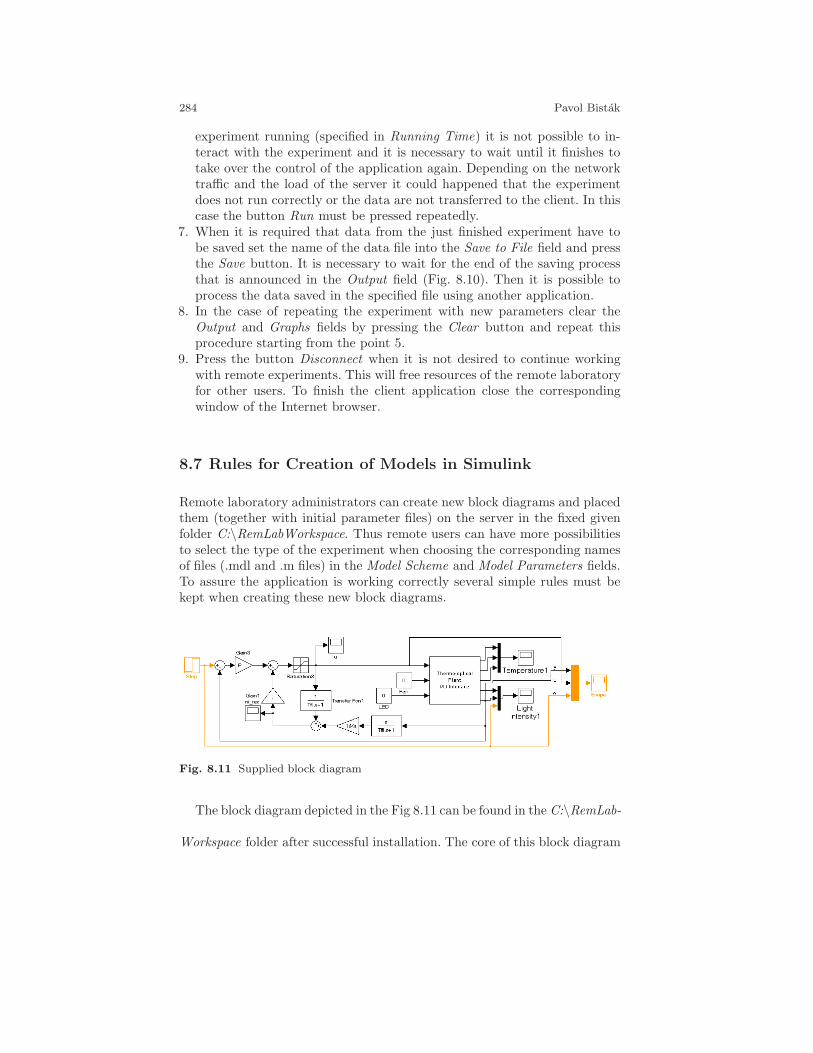
284 Pavol Bistak
experiment running (specified in Running Time) it is not possible to in-teract with the experiment and it is necessary to wait until it finishes totake over the control of the application again. Depending on the networktraffic and the load of the server it could happened that the experimentdoes not run correctly or the data are not transferred to the client. In thiscase the button Run must be pressed repeatedly.
7. When it is required that data from the just finished experiment have tobe saved set the name of the data file into the Save to File field and pressthe Save button. It is necessary to wait for the end of the saving processthat is announced in the Output field (Fig. 8.10). Then it is possible toprocess the data saved in the specified file using another application.
8. In the case of repeating the experiment with new parameters clear theOutput and Graphs fields by pressing the Clear button and repeat thisprocedure starting from the point 5.
9. Press the button Disconnect when it is not desired to continue workingwith remote experiments. This will free resources of the remote laboratoryfor other users. To finish the client application close the correspondingwindow of the Internet browser.
8.7 Rules for Creation of Models in Simulink
Remote laboratory administrators can create new block diagrams and placedthem (together with initial parameter files) on the server in the fixed givenfolder C:\RemLabWorkspace. Thus remote users can have more possibilitiesto select the type of the experiment when choosing the corresponding namesof files (.mdl and .m files) in the Model Scheme and Model Parameters fields.To assure the application is working correctly several simple rules must bekept when creating these new block diagrams.
Fig. 8.11 Supplied block diagram
The block diagram depicted in the Fig 8.11 can be found in the C:\RemLab-
Workspace folder after successful installation. The core of this block diagram
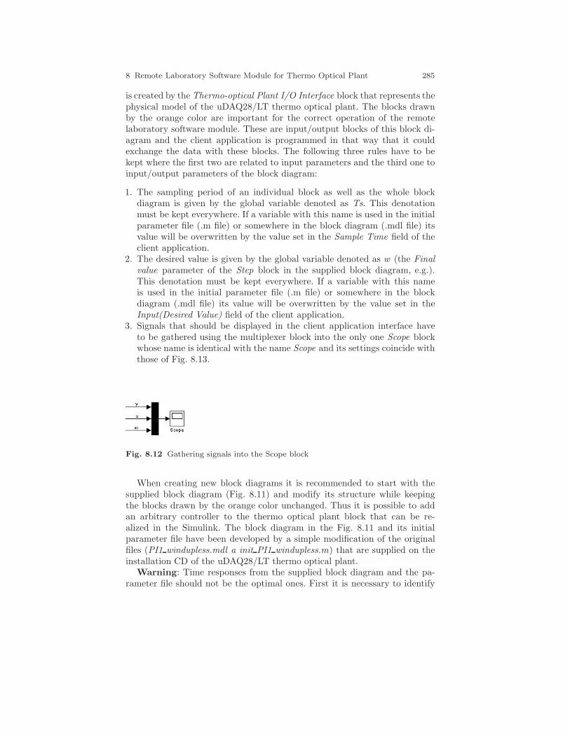
8 Remote Laboratory Software Module for Thermo Optical Plant 285
is created by the Thermo-optical Plant I/O Interface block that represents thephysical model of the uDAQ28/LT thermo optical plant. The blocks drawnby the orange color are important for the correct operation of the remotelaboratory software module. These are input/output blocks of this block di-agram and the client application is programmed in that way that it couldexchange the data with these blocks. The following three rules have to bekept where the first two are related to input parameters and the third one toinput/output parameters of the block diagram:
1. The sampling period of an individual block as well as the whole blockdiagram is given by the global variable denoted as Ts. This denotationmust be kept everywhere. If a variable with this name is used in the initialparameter file (.m file) or somewhere in the block diagram (.mdl file) itsvalue will be overwritten by the value set in the Sample Time field of theclient application.
2. The desired value is given by the global variable denoted as w (the Finalvalue parameter of the Step block in the supplied block diagram, e.g.).This denotation must be kept everywhere. If a variable with this nameis used in the initial parameter file (.m file) or somewhere in the blockdiagram (.mdl file) its value will be overwritten by the value set in theInput(Desired Value) field of the client application.
3. Signals that should be displayed in the client application interface haveto be gathered using the multiplexer block into the only one Scope blockwhose name is identical with the name Scope and its settings coincide withthose of Fig. 8.13.
Fig. 8.12 Gathering signals into the Scope block
When creating new block diagrams it is recommended to start with thesupplied block diagram (Fig. 8.11) and modify its structure while keepingthe blocks drawn by the orange color unchanged. Thus it is possible to addan arbitrary controller to the thermo optical plant block that can be re-alized in the Simulink. The block diagram in the Fig. 8.11 and its initialparameter file have been developed by a simple modification of the originalfiles (PI1 windupless.mdl a init PI1 windupless.m) that are supplied on theinstallation CD of the uDAQ28/LT thermo optical plant.
Warning: Time responses from the supplied block diagram and the pa-rameter file should not be the optimal ones. First it is necessary to identify
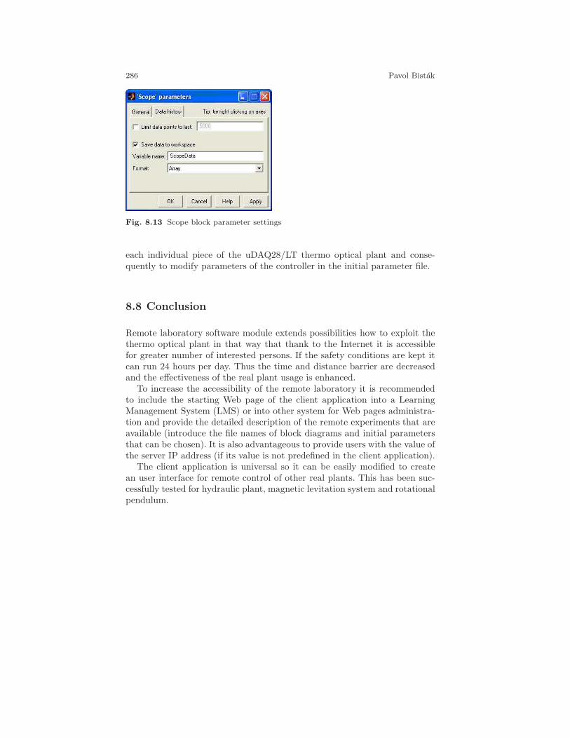
286 Pavol Bistak
Fig. 8.13 Scope block parameter settings
each individual piece of the uDAQ28/LT thermo optical plant and conse-quently to modify parameters of the controller in the initial parameter file.
8.8 Conclusion
Remote laboratory software module extends possibilities how to exploit thethermo optical plant in that way that thank to the Internet it is accessiblefor greater number of interested persons. If the safety conditions are kept itcan run 24 hours per day. Thus the time and distance barrier are decreasedand the effectiveness of the real plant usage is enhanced.
To increase the accessibility of the remote laboratory it is recommendedto include the starting Web page of the client application into a LearningManagement System (LMS) or into other system for Web pages administra-tion and provide the detailed description of the remote experiments that areavailable (introduce the file names of block diagrams and initial parametersthat can be chosen). It is also advantageous to provide users with the value ofthe server IP address (if its value is not predefined in the client application).
The client application is universal so it can be easily modified to createan user interface for remote control of other real plants. This has been suc-cessfully tested for hydraulic plant, magnetic levitation system and rotationalpendulum.

8 Remote Laboratory Software Module for Thermo Optical Plant 287
Comments – Remarks

288 Pavol Bistak
Comments – Remarks

8 Remote Laboratory Software Module for Thermo Optical Plant 289
Comments – Remarks

290 Pavol Bistak
Comments – Remarks
Chapter 9
Constrained PID controlTasks for Controlling the Thermo OpticalPlant
Peter Tapak and Mikulas Huba
Abstract Tuning of simple controllers respecting input constraints will beconsidered in this chapter and verified by controlling simple physical deviceof thermo-optical plant. The chapter starts with short user’s manual andinstallation guide to the uDAQ28/LT device which will be used as a realplant to apply the control on. In the introduction, several fundamental con-trollers of the Dynamical class 0 (DC0) will be considered that avoid controlsaturation by guaranteeing monotonic transients among steady states at thecontroller output. Processes of the DC0 are typically met in situations, wherethe dynamics of transients may be neglected, i.e. it is not connected with areasonable energy accumulation. In such cases, the ideal control responsefollowing a setpoint step may also converge to step function (not having asaturation phase). Controllers of the DC0 may also be successfully appliedto any stable plant, but in such situations it is no more possible to speed upthe control signal transient up to the step function, just to keep it monotonicthat guarantees that all such controllers may again be successfully treatedby the linear theory as well. In the second part, basic structures of the DC1will be introduced that may already typically have one constrained periodin their control signal step responses. Here, control structures with integralaction based on disturbance observers will be introduced that do not exhibitwindup phenomenon and so enable simpler one-step tuning that in the caseof traditional linear controllers extended by the anti-windup circuitry.
Peter TapakInstitute of Control and Industrial InformaticsFaculty of Electrical Engineering and IT, Slovak University of TechnologyIlkovicova 3, 812 19 Bratislava, Slovakia, e-mail: [email protected]
Mikulas HubaInstitute of Control and Industrial InformaticsFaculty of Electrical Engineering and IT, Slovak University of TechnologyIlkovicova 3, 812 19 Bratislava, Slovakia, e-mail: [email protected]
291
292 Peter Tapak and Mikulas Huba
9.1 Thermo-optical Plant uDAQ28/LT – Quick Start
This section gives a short guide to uDAQ28/LT plant. Get familiar withthermo-optical plant interface. For more information on the device please re-fer to the user’s manual. This device offers measurement of eighth processvariables (temperature and its filtered value, ambient temperature, light in-tensity, its filtered value and its derivative, the ventilator speed of rotationand its motor current). The temperature and the light intensity control chan-nels are interconnected by three manipulated variables: the bulb voltage (theheat and light source), the light-diode voltage (the light source) and the ven-tilator voltage (the system cooling). The plant can be easily connected tostandard computers via USB, when it enables to work with the sampling pe-riods 40-50 ms and larger. Within the Matlab/Simulink scheme the plant isrepresented as a single block, limiting use of costly and complicated softwarepackage for the real time control.
9.1.1 Installation in Windows Operating System
9.1.1.1 Device Driver Installation
New hardware is detected automatically by operating system and Found NewHardware Wizard will start after plugging device into electrical power networkand connecting it to PC by USB cable (Fig. 9.1). Choose driver installationfrom specific location (Fig. 9.2)
Directory driver from the package of supporting software is needed toselect as device driver location path (Fig. 9.3). Complete installation requirestwo cycles of adding new hardware (USB Serial Converter and USB SerialPort is installed into operating system, Found New Hardware Wizard startsautomatically second time). The user is informed on successful completion ofinstallation, see the window on the Fig. 9.4.
When the device has been installed, (virtual) serial port is available onthe list of hardware devices, labeled as USB Serial Port. One can get to itssettings through Device Manager (Start / Settings / Control Panel / System/ Hardware / Device Manager ) if Ports (COM & LPT) / USB Serial Port isselected (Fig. 9.5). The port has automatically assigned by the system one ofcom port numbers (which is not in use). If the assigned number is bigger than4, it is necessary to change it to different com port number from the range1-4, which is not in use at the moment. It is possible to perform on the tabPort Settings / Advanced / COM Port Number (Fig. 9.6). The last actionafter installation to be done is setting parameter Latency Timer (msec) onvalue 1, which minimizes data loss during data transfer. Parameter LatencyTimer (msec) is available on the same tab as COM Port Number (Fig. 9.6).In the case that all com port numbers from the range 1-4 are already in use by

9 Constrained PID control Tasks for Controlling the Thermo Optical Plant 293
Fig. 9.1 Found new hardware wizard
Fig. 9.2 Install driver from specific location selection
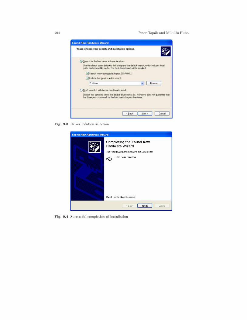
294 Peter Tapak and Mikulas Huba
Fig. 9.3 Driver location selection
Fig. 9.4 Successful completion of installation
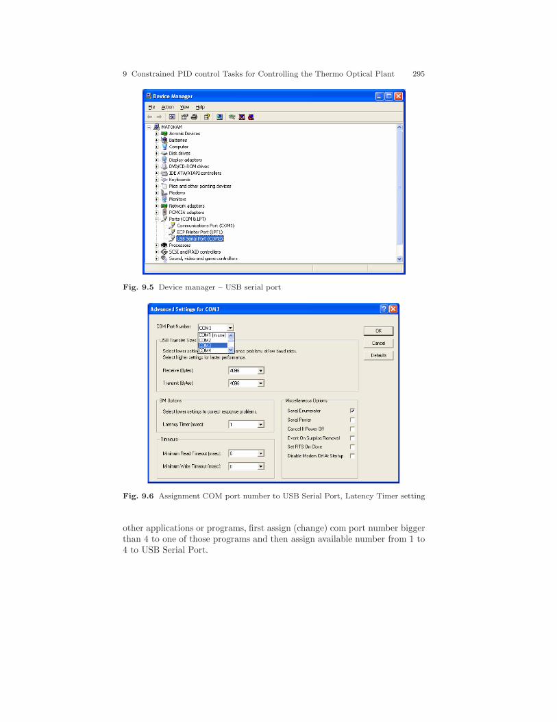
9 Constrained PID control Tasks for Controlling the Thermo Optical Plant 295
Fig. 9.5 Device manager – USB serial port
Fig. 9.6 Assignment COM port number to USB Serial Port, Latency Timer setting
other applications or programs, first assign (change) com port number biggerthan 4 to one of those programs and then assign available number from 1 to4 to USB Serial Port.
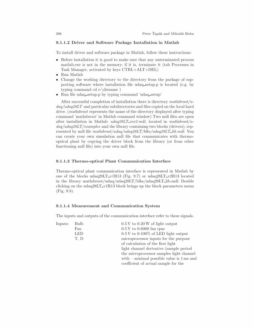
296 Peter Tapak and Mikulas Huba
9.1.1.2 Driver and Software Package Installation in Matlab
To install driver and software package in Matlab, follow these instructions:
• Before installation it is good to make sure that any unterminated processmatlab.exe is not in the memory; if it is, terminate it (tab Processes inTask Manager, activated by keys CTRL+ALT+DEL)
• Run Matlab• Change the working directory to the directory from the package of sup-
porting software where installation file udaq setup.p is located (e.g. bytyping command cd e:\dirname )
• Run file udaq setup.p by typing command ’udaq setup’
After successful completion of installation there is directory matlabroot/u-daq/udaq28LT and particular subdirectories and files copied on the local harddrive. (matlabroot represents the name of the directory displayed after typingcommand ’matlabroot’ in Matlab command window) Two mdl files are openafter installation in Matlab: udaq28LT iov2.mdl, located in matlabroot/u-daq/udaq28LT/examples and the library containing two blocks (drivers), rep-resented by mdl file matlabroot/udaq/udaq28LT/blks/udaq28LT lib.mdl. Youcan create your own simulation mdl file that communicates with thermo-optical plant by copying the driver block from the library (or from otherfunctioning mdl file) into your own mdl file.
9.1.1.3 Thermo-optical Plant Communication Interface
Thermo-optical plant communication interface is represented in Matlab byone of the blocks udaq28LT v1R13 (Fig. 9.7) or udaq28LT v2R13 locatedin the library matlabroot/udaq/udaq28LT/blks/udaq28LT lib.mdl. Doubleclicking on the udaq28LT v1R13 block brings up the block parameters menu(Fig. 9.8).
9.1.1.4 Measurement and Communication System
The inputs and outputs of the communication interface refer to these signals.
Inputs: Bulb 0-5V to 0-20W of light outputFan 0-5V to 0-6000 fan rpmLED 0-5V to 0-100% of LED light outputT, D microprocessor inputs for the purpose
of calculation of the first lightlight channel derivative (sample periodthe microprocessor samples light channelwith – minimal possible value is 1ms andcoefficient of actual sample for the
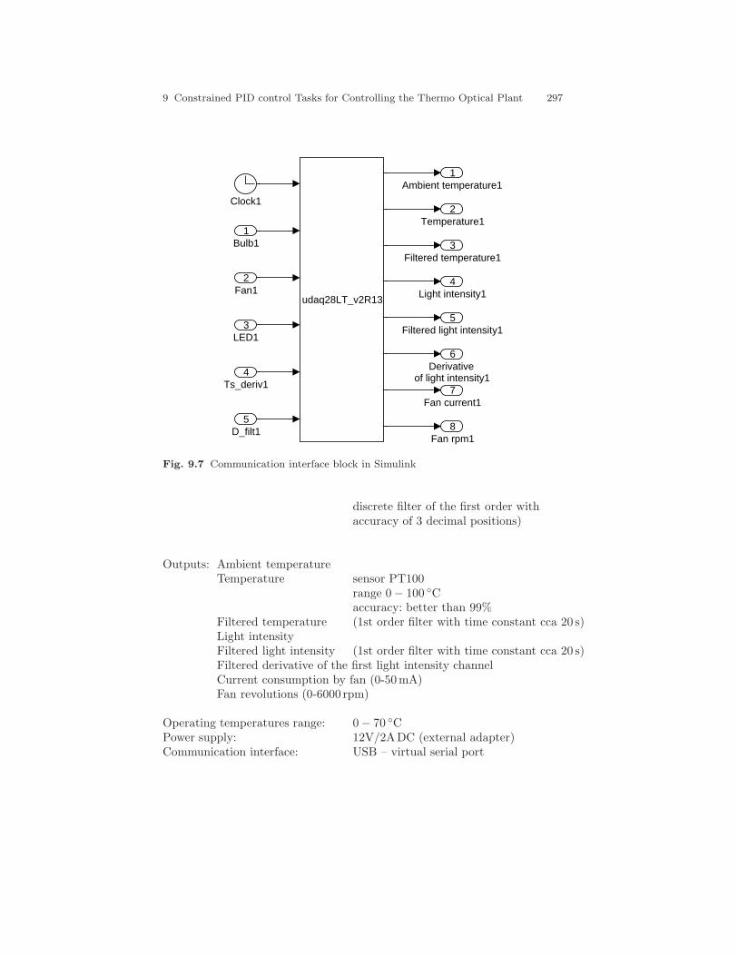
9 Constrained PID control Tasks for Controlling the Thermo Optical Plant 297
8Fan rpm1
7Fan current1
6Derivative
of light intensity1
5Filtered light intensity1
4Light intensity1
3Filtered temperature1
2Temperature1
1Ambient temperature1
udaq28LT_v2R13
Clock1
5D_filt1
4Ts_deriv1
3LED1
2Fan1
1Bulb1
Fig. 9.7 Communication interface block in Simulink
discrete filter of the first order withaccuracy of 3 decimal positions)
Outputs: Ambient temperatureTemperature sensor PT100
range 0− 100 Caccuracy: better than 99%
Filtered temperature (1st order filter with time constant cca 20 s)Light intensityFiltered light intensity (1st order filter with time constant cca 20 s)Filtered derivative of the first light intensity channelCurrent consumption by fan (0-50mA)Fan revolutions (0-6000 rpm)
Operating temperatures range: 0− 70 CPower supply: 12V/2ADC (external adapter)Communication interface: USB – virtual serial port

298 Peter Tapak and Mikulas Huba
Fig. 9.8 User dialog window of communication interface
Data transfer speed: 250 kbit/s
9.2 Light Channel Control
The non-filtered and filtered light channels of uDAQ/28LT plant are goingto be controlled in this section. Simple alternatives to linear I-controllers willbe practiced.
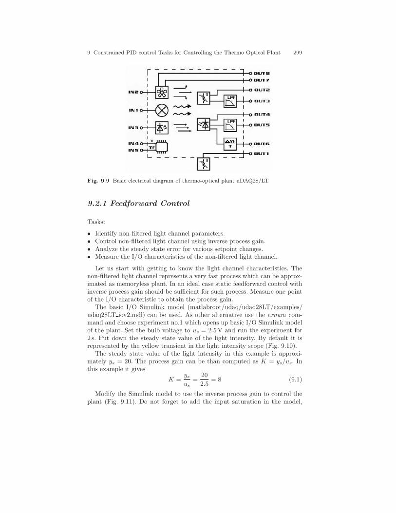
9 Constrained PID control Tasks for Controlling the Thermo Optical Plant 299
Fig. 9.9 Basic electrical diagram of thermo-optical plant uDAQ28/LT
9.2.1 Feedforward Control
Tasks:
• Identify non-filtered light channel parameters.• Control non-filtered light channel using inverse process gain.• Analyze the steady state error for various setpoint changes.• Measure the I/O characteristics of the non-filtered light channel.
Let us start with getting to know the light channel characteristics. Thenon-filtered light channel represents a very fast process which can be approx-imated as memoryless plant. In an ideal case static feedforward control withinverse process gain should be sufficient for such process. Measure one pointof the I/O characteristic to obtain the process gain.
The basic I/O Simulink model (matlabroot/udaq/udaq28LT/examples/udaq28LT iov2.mdl) can be used. As other alternative use the exnum com-mand and choose experiment no.1 which opens up basic I/O Simulink modelof the plant. Set the bulb voltage to us = 2.5V and run the experiment for2 s. Put down the steady state value of the light intensity. By default it isrepresented by the yellow transient in the light intensity scope (Fig. 9.10).
The steady state value of the light intensity in this example is approxi-mately ys = 20. The process gain can be than computed as K = ys/us. Inthis example it gives
K =ysus
=20
2.5= 8 (9.1)
Modify the Simulink model to use the inverse process gain to control theplant (Fig. 9.11). Do not forget to add the input saturation in the model,
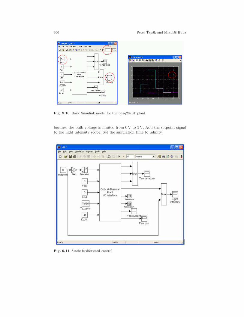
300 Peter Tapak and Mikulas Huba
Fig. 9.10 Basic Simulink model for the udaq28/LT plant
because the bulb voltage is limited from 0V to 5V. Add the setpoint signalto the light intensity scope. Set the simulation time to infinity.
Fig. 9.11 Static feedforward control
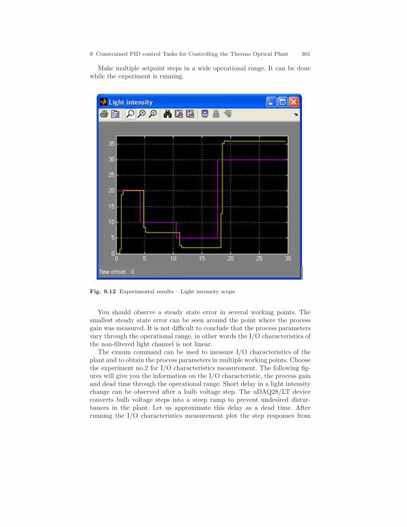
9 Constrained PID control Tasks for Controlling the Thermo Optical Plant 301
Make multiple setpoint steps in a wide operational range. It can be donewhile the experiment is running.
Fig. 9.12 Experimental results – Light intensity scope
You should observe a steady state error in several working points. Thesmallest steady state error can be seen around the point where the processgain was measured. It is not difficult to conclude that the process parametersvary through the operational range, in other words the I/O characteristics ofthe non-filtered light channel is not linear.
The exnum command can be used to measure I/O characteristics of theplant and to obtain the process parameters in multiple working points. Choosethe experiment no.2 for I/O characteristics measurement. The following fig-ures will give you the information on the I/O characteristic, the process gainand dead time through the operational range. Short delay in a light intensitychange can be observed after a bulb voltage step. The uDAQ28/LT deviceconverts bulb voltage steps into a steep ramp to prevent undesired distur-bances in the plant. Let us approximate this delay as a dead time. Afterrunning the I/O characteristics measurement plot the step responses from
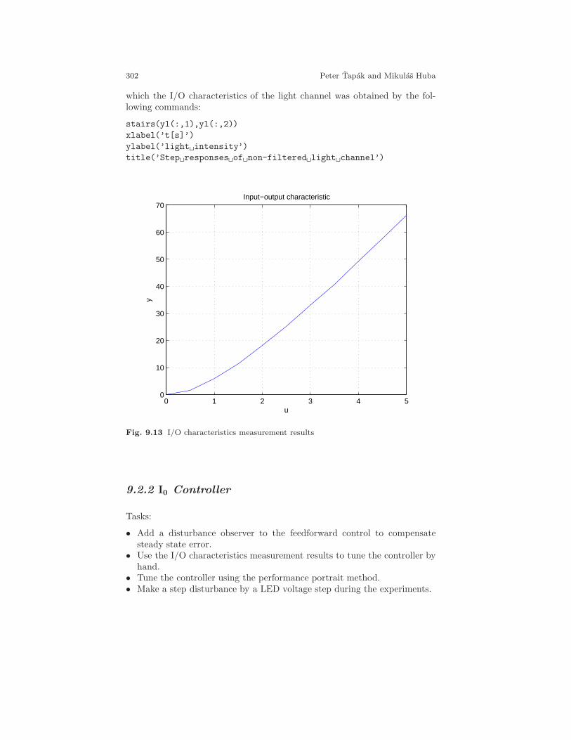
302 Peter Tapak and Mikulas Huba
which the I/O characteristics of the light channel was obtained by the fol-lowing commands:
stairs(yl(:,1),yl(:,2))
xlabel(’t[s]’)
ylabel(’light intensity’)
title(’Step responses of non-filtered light channel’)
0 1 2 3 4 50
10
20
30
40
50
60
70Input−output characteristic
u
y
Fig. 9.13 I/O characteristics measurement results
9.2.2 I0 Controller
Tasks:
• Add a disturbance observer to the feedforward control to compensatesteady state error.
• Use the I/O characteristics measurement results to tune the controller byhand.
• Tune the controller using the performance portrait method.• Make a step disturbance by a LED voltage step during the experiments.
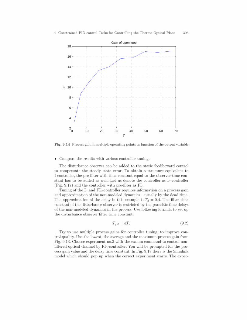
9 Constrained PID control Tasks for Controlling the Thermo Optical Plant 303
0 10 20 30 40 50 60 702
4
6
8
10
12
14
16
18Gain of open loop
y
K
Fig. 9.14 Process gain in multiple operating points as function of the output variable
• Compare the results with various controller tuning.
The disturbance observer can be added to the static feedforward controlto compensate the steady state error. To obtain a structure equivalent toI-controller, the pre-filter with time constant equal to the observer time con-stant has to be added as well. Let us denote the controller as I0-controller(Fig. 9.17) and the controller with pre-filter as FI0.
Tuning of the I0 and FI0-controller requires information on a process gainand approximation of the non-modeled dynamics – usually by the dead time.The approximation of the delay in this example is Td = 0.4. The filter timeconstant of the disturbance observer is restricted by the parasitic time delaysof the non-modeled dynamics in the process. Use following formula to set upthe disturbance observer filter time constant:
Tfil = eTd (9.2)
Try to use multiple process gains for controller tuning, to improve con-trol quality. Use the lowest, the average and the maximum process gain fromFig. 9.13. Choose experiment no.3 with the exnum command to control non-filtered optical channel by FI0-controller. You will be prompted for the pro-cess gain value and the delay time constant. In Fig. 9.18 there is the Simulinkmodel which should pop up when the correct experiment starts. The exper-
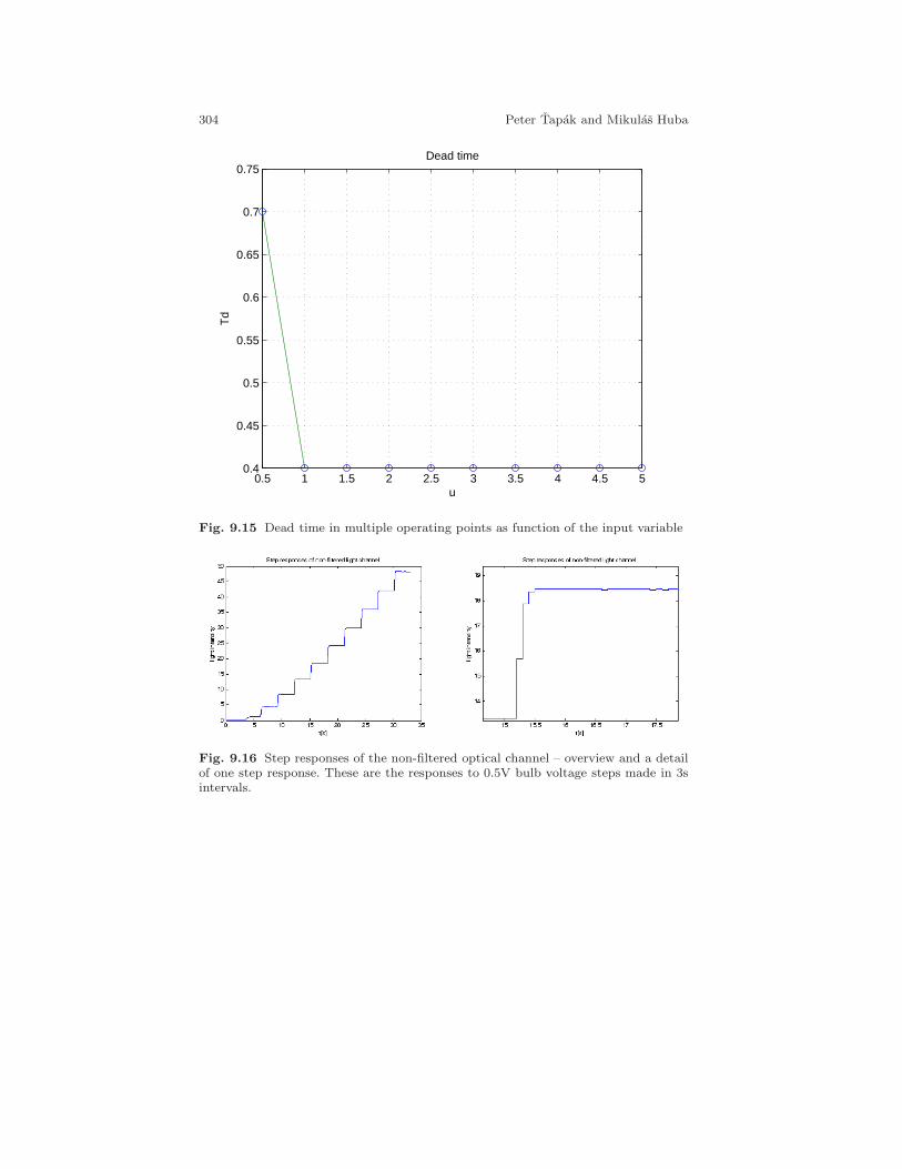
304 Peter Tapak and Mikulas Huba
0.5 1 1.5 2 2.5 3 3.5 4 4.5 50.4
0.45
0.5
0.55
0.6
0.65
0.7
0.75Dead time
u
Td
Fig. 9.15 Dead time in multiple operating points as function of the input variable
Fig. 9.16 Step responses of the non-filtered optical channel – overview and a detailof one step response. These are the responses to 0.5V bulb voltage steps made in 3sintervals.
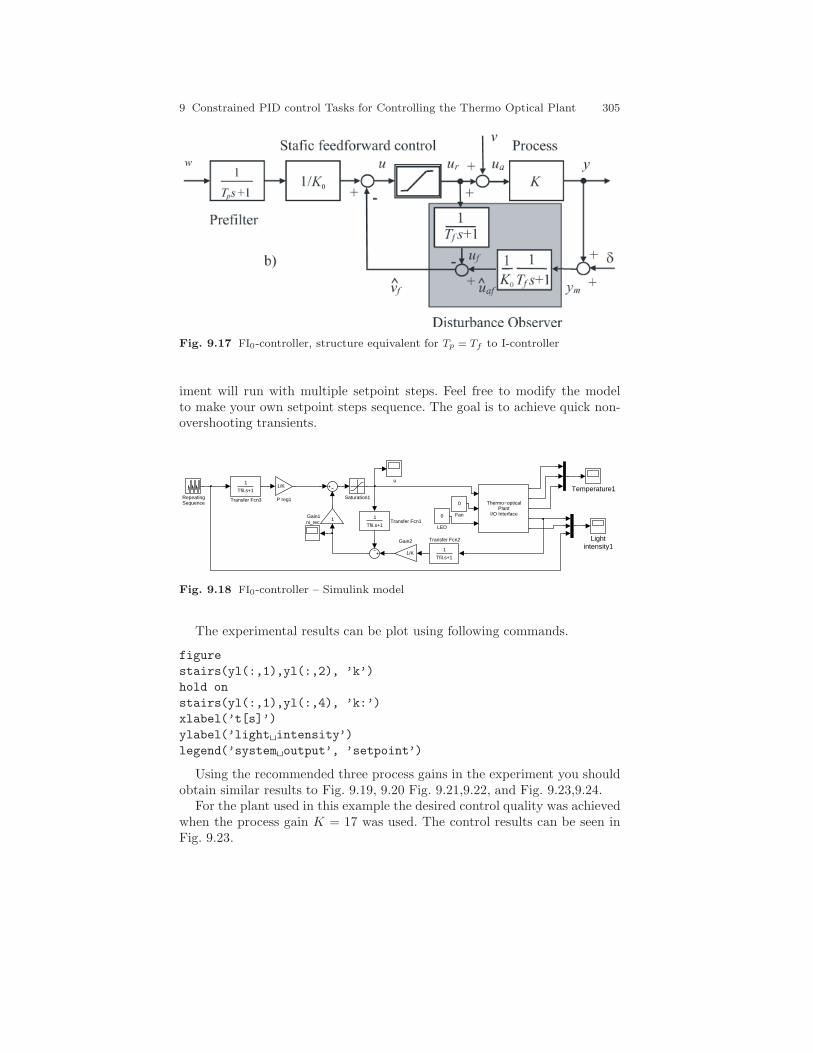
9 Constrained PID control Tasks for Controlling the Thermo Optical Plant 305
Fig. 9.17 FI0-controller, structure equivalent for Tp = Tf to I-controller
iment will run with multiple setpoint steps. Feel free to modify the modelto make your own setpoint steps sequence. The goal is to achieve quick non-overshooting transients.
u
ni_rec
1
Tfil.s+1
Transfer Fcn3
1
Tfil.s+1
Transfer Fcn2
1
Tfil.s+1Transfer Fcn1
Thermo−opticalPlant
I/O Interface
Temperature1Saturation1Repeating
Sequence
1/K
P reg1
Lightintensity1
0
LED
1/K
Gain2
1Gain1
0
Fan
Fig. 9.18 FI0-controller – Simulink model
The experimental results can be plot using following commands.
figure
stairs(yl(:,1),yl(:,2), ’k’)
hold on
stairs(yl(:,1),yl(:,4), ’k:’)
xlabel(’t[s]’)
ylabel(’light intensity’)
legend(’system output’, ’setpoint’)
Using the recommended three process gains in the experiment you shouldobtain similar results to Fig. 9.19, 9.20 Fig. 9.21,9.22, and Fig. 9.23,9.24.
For the plant used in this example the desired control quality was achievedwhen the process gain K = 17 was used. The control results can be seen inFig. 9.23.
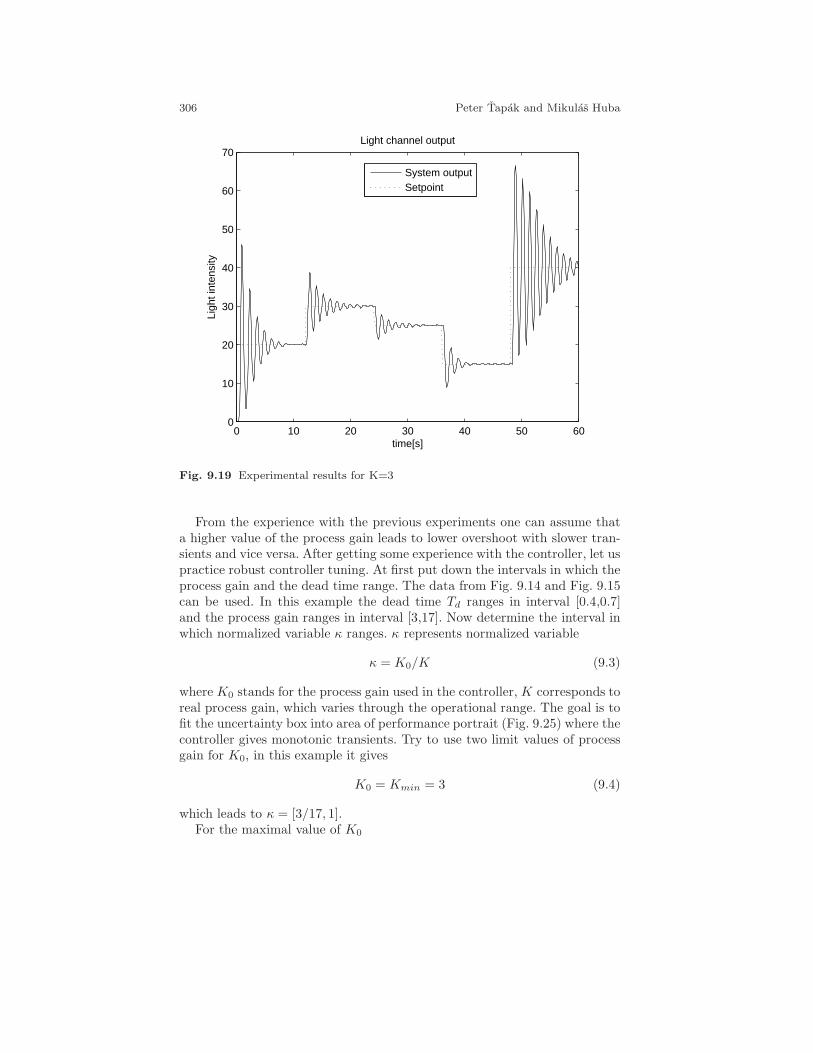
306 Peter Tapak and Mikulas Huba
0 10 20 30 40 50 600
10
20
30
40
50
60
70
time[s]
Ligh
t int
ensi
ty
Light channel output
System outputSetpoint
Fig. 9.19 Experimental results for K=3
From the experience with the previous experiments one can assume thata higher value of the process gain leads to lower overshoot with slower tran-sients and vice versa. After getting some experience with the controller, let uspractice robust controller tuning. At first put down the intervals in which theprocess gain and the dead time range. The data from Fig. 9.14 and Fig. 9.15can be used. In this example the dead time Td ranges in interval [0.4,0.7]and the process gain ranges in interval [3,17]. Now determine the interval inwhich normalized variable κ ranges. κ represents normalized variable
κ = K0/K (9.3)
where K0 stands for the process gain used in the controller, K corresponds toreal process gain, which varies through the operational range. The goal is tofit the uncertainty box into area of performance portrait (Fig. 9.25) where thecontroller gives monotonic transients. Try to use two limit values of processgain for K0, in this example it gives
K0 = Kmin = 3 (9.4)
which leads to κ = [3/17, 1].For the maximal value of K0
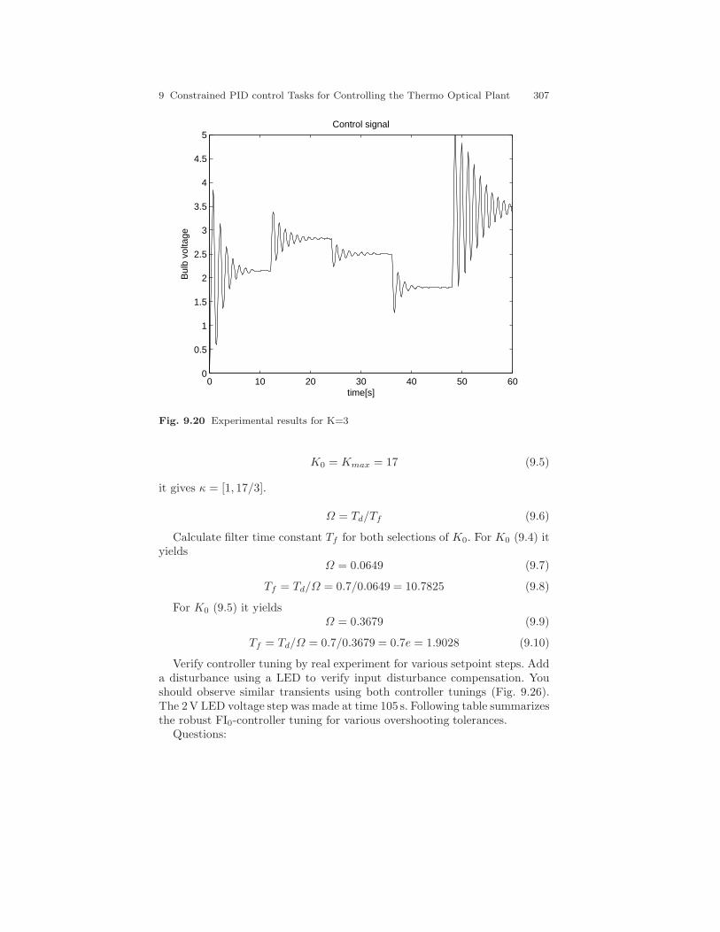
9 Constrained PID control Tasks for Controlling the Thermo Optical Plant 307
0 10 20 30 40 50 600
0.5
1
1.5
2
2.5
3
3.5
4
4.5
5
time[s]
Control signal
Bul
b vo
ltage
Fig. 9.20 Experimental results for K=3
K0 = Kmax = 17 (9.5)
it gives κ = [1, 17/3].
Ω = Td/Tf (9.6)
Calculate filter time constant Tf for both selections of K0. For K0 (9.4) ityields
Ω = 0.0649 (9.7)
Tf = Td/Ω = 0.7/0.0649 = 10.7825 (9.8)
For K0 (9.5) it yieldsΩ = 0.3679 (9.9)
Tf = Td/Ω = 0.7/0.3679 = 0.7e = 1.9028 (9.10)
Verify controller tuning by real experiment for various setpoint steps. Adda disturbance using a LED to verify input disturbance compensation. Youshould observe similar transients using both controller tunings (Fig. 9.26).The 2V LED voltage step was made at time 105 s. Following table summarizesthe robust FI0-controller tuning for various overshooting tolerances.
Questions:
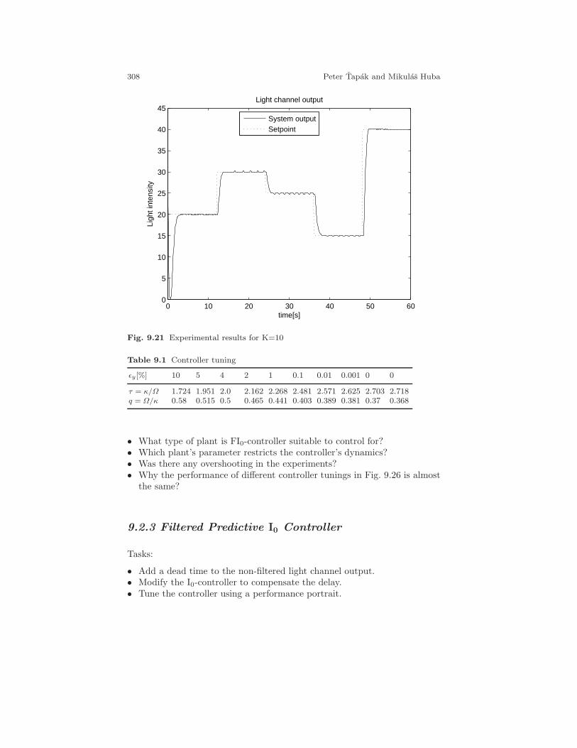
308 Peter Tapak and Mikulas Huba
0 10 20 30 40 50 600
5
10
15
20
25
30
35
40
45
time[s]
Ligh
t int
ensi
ty
Light channel output
System outputSetpoint
Fig. 9.21 Experimental results for K=10
Table 9.1 Controller tuning
ǫy[%] 10 5 4 2 1 0.1 0.01 0.001 0 0
τ = κ/Ω 1.724 1.951 2.0 2.162 2.268 2.481 2.571 2.625 2.703 2.718q = Ω/κ 0.58 0.515 0.5 0.465 0.441 0.403 0.389 0.381 0.37 0.368
• What type of plant is FI0-controller suitable to control for?• Which plant’s parameter restricts the controller’s dynamics?• Was there any overshooting in the experiments?• Why the performance of different controller tunings in Fig. 9.26 is almost
the same?
9.2.3 Filtered Predictive I0 Controller
Tasks:
• Add a dead time to the non-filtered light channel output.• Modify the I0-controller to compensate the delay.• Tune the controller using a performance portrait.
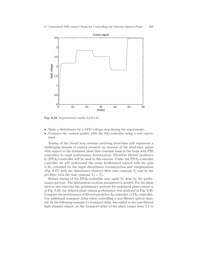
9 Constrained PID control Tasks for Controlling the Thermo Optical Plant 309
0 10 20 30 40 50 600
0.5
1
1.5
2
2.5
3
3.5
time[s]
Control signal
Bul
b vo
ltage
Fig. 9.22 Experimental results for K=10
• Make a disturbance by a LED voltage step during the experiments.• Compare the control quality with the FI0-controller using a real experi-
ment.
Tuning of the closed loop systems involving dead-time still represents achallenging domain of control research. an increase of the dead-time valueswith respect to the dominant plant time constant leads in the loops with PIDcontrollers to rapid performance deterioration. Therefore filtered predictiveI0 (FPrI0)-controller will be used in this exercise. Under the FPrI0-controllercontroller we will understand the static feedforward control with the gain1/K0 extended by the input disturbance reconstruction and compensation(Fig. 9.27) with the disturbance observer filter time constant Tf and by thepre-filter with the time constant Tp = Tf .
Robust tuning of the FPrI0-controller may again be done by the perfor-mance portrait. The information on plant parameters is needed. For the plantused in this exercises the performance portrait for undelayed plant output isin Fig. 9.29, the delayed plant output performance was analyzed in Fig. 9.30.Compare the performance of filtered predictive I0-controller vs FI0-controller.Use additional transport delay when controlling a non-filtered optical chan-nel. In the following example 5 s transport delay was added to the non-filteredlight channel output, so the transport delay of the plant ranges from 5.4 to
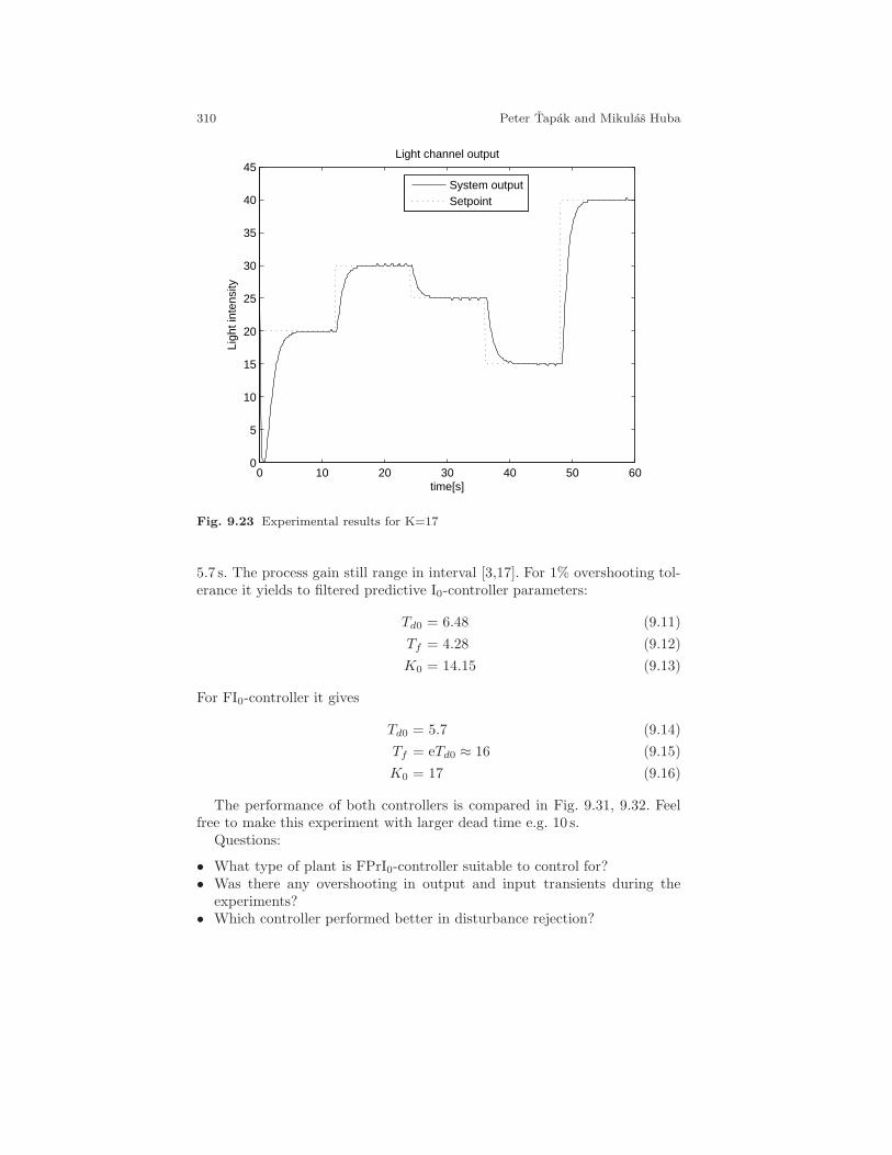
310 Peter Tapak and Mikulas Huba
0 10 20 30 40 50 600
5
10
15
20
25
30
35
40
45
time[s]
Ligh
t int
ensi
ty
Light channel output
System outputSetpoint
Fig. 9.23 Experimental results for K=17
5.7 s. The process gain still range in interval [3,17]. For 1% overshooting tol-erance it yields to filtered predictive I0-controller parameters:
Td0 = 6.48 (9.11)
Tf = 4.28 (9.12)
K0 = 14.15 (9.13)
For FI0-controller it gives
Td0 = 5.7 (9.14)
Tf = eTd0 ≈ 16 (9.15)
K0 = 17 (9.16)
The performance of both controllers is compared in Fig. 9.31, 9.32. Feelfree to make this experiment with larger dead time e.g. 10 s.
Questions:
• What type of plant is FPrI0-controller suitable to control for?• Was there any overshooting in output and input transients during the
experiments?• Which controller performed better in disturbance rejection?
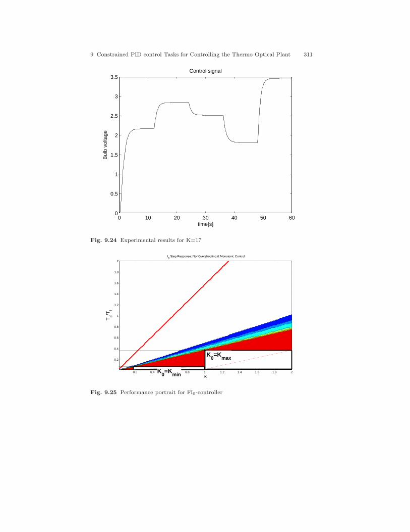
9 Constrained PID control Tasks for Controlling the Thermo Optical Plant 311
0 10 20 30 40 50 600
0.5
1
1.5
2
2.5
3
3.5
time[s]
Control signal
Bul
b vo
ltage
Fig. 9.24 Experimental results for K=17
0.2 0.4 0.6 0.8 1 1.2 1.4 1.6 1.8 2
0.2
0.4
0.6
0.8
1
1.2
1.4
1.6
1.8
2
I0 Step Response: NonOvershooting & Monotonic Control
Td/T
f
κK
0=K
min
K0=K
max
Fig. 9.25 Performance portrait for FI0-controller
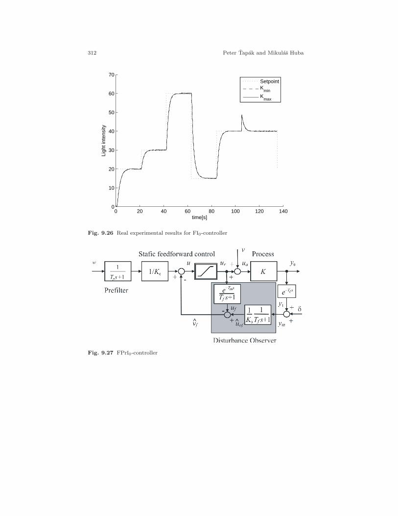
312 Peter Tapak and Mikulas Huba
0 20 40 60 80 100 120 1400
10
20
30
40
50
60
70
time[s]
Ligh
t int
ensi
ty
SetpointK
minK
max
Fig. 9.26 Real experimental results for FI0-controller
Fig. 9.27 FPrI0-controller
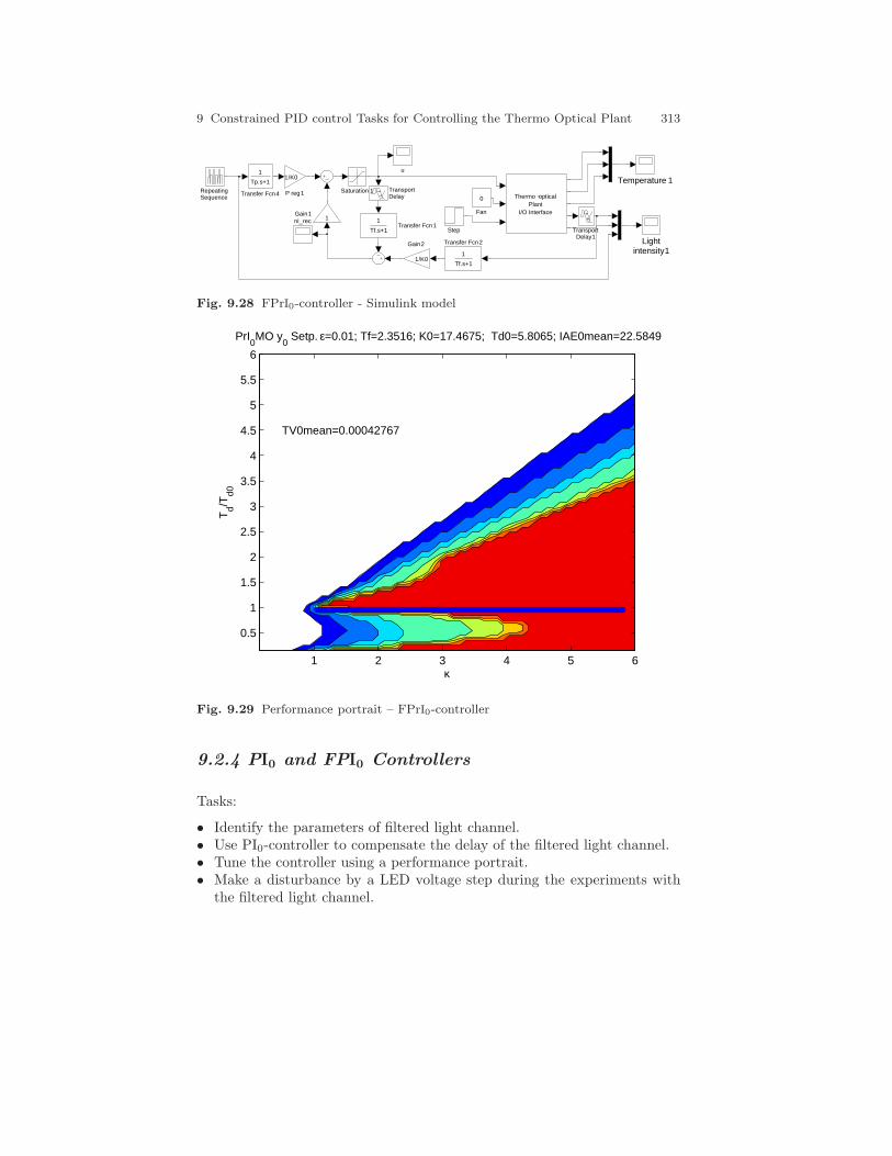
9 Constrained PID control Tasks for Controlling the Thermo Optical Plant 313
u
ni_rec
TransportDelay1
TransportDelayTransfer Fcn4
1
Tp.s+1
Transfer Fcn2
1
Tf.s+1
Transfer Fcn11
Tf.s+1
Thermo −opticalPlant
I/O Interface
Temperature 1
Step
Saturation 1RepeatingSequence
P reg1
1/K0
Lightintensity1
Gain2
1/K0
Gain11
Fan
0
Fig. 9.28 FPrI0-controller - Simulink model
Td/T
d0
κ
PrI0MO y
0 Setp. ε=0.01; Tf=2.3516; K0=17.4675; Td0=5.8065; IAE0mean=22.5849
TV0mean=0.00042767
1 2 3 4 5 6
0.5
1
1.5
2
2.5
3
3.5
4
4.5
5
5.5
6
Fig. 9.29 Performance portrait – FPrI0-controller
9.2.4 PI0 and FPI0 Controllers
Tasks:
• Identify the parameters of filtered light channel.• Use PI0-controller to compensate the delay of the filtered light channel.• Tune the controller using a performance portrait.• Make a disturbance by a LED voltage step during the experiments with
the filtered light channel.
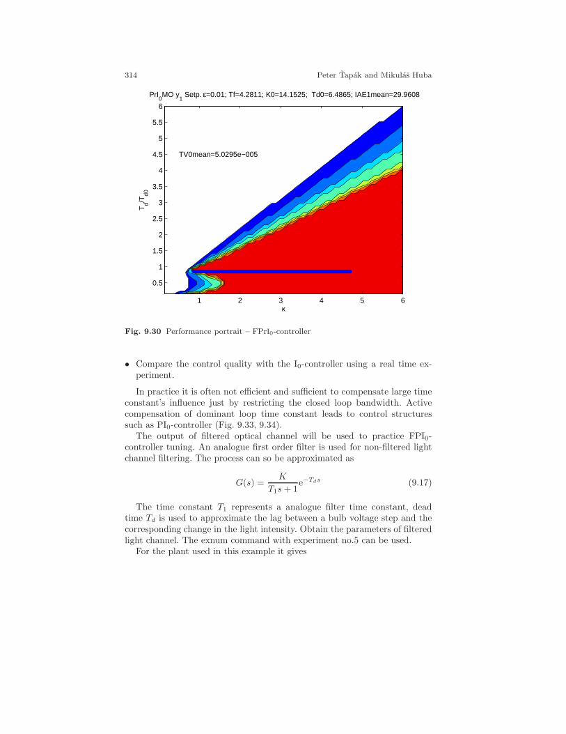
314 Peter Tapak and Mikulas Huba
Td/T
d0
κ
PrI0MO y
1 Setp. ε=0.01; Tf=4.2811; K0=14.1525; Td0=6.4865; IAE1mean=29.9608
TV0mean=5.0295e−005
1 2 3 4 5 6
0.5
1
1.5
2
2.5
3
3.5
4
4.5
5
5.5
6
Fig. 9.30 Performance portrait – FPrI0-controller
• Compare the control quality with the I0-controller using a real time ex-periment.
In practice it is often not efficient and sufficient to compensate large timeconstant’s influence just by restricting the closed loop bandwidth. Activecompensation of dominant loop time constant leads to control structuressuch as PI0-controller (Fig. 9.33, 9.34).
The output of filtered optical channel will be used to practice FPI0-controller tuning. An analogue first order filter is used for non-filtered lightchannel filtering. The process can so be approximated as
G(s) =K
T1s+ 1e−Tds (9.17)
The time constant T1 represents a analogue filter time constant, deadtime Td is used to approximate the lag between a bulb voltage step and thecorresponding change in the light intensity. Obtain the parameters of filteredlight channel. The exnum command with experiment no.5 can be used.
For the plant used in this example it gives
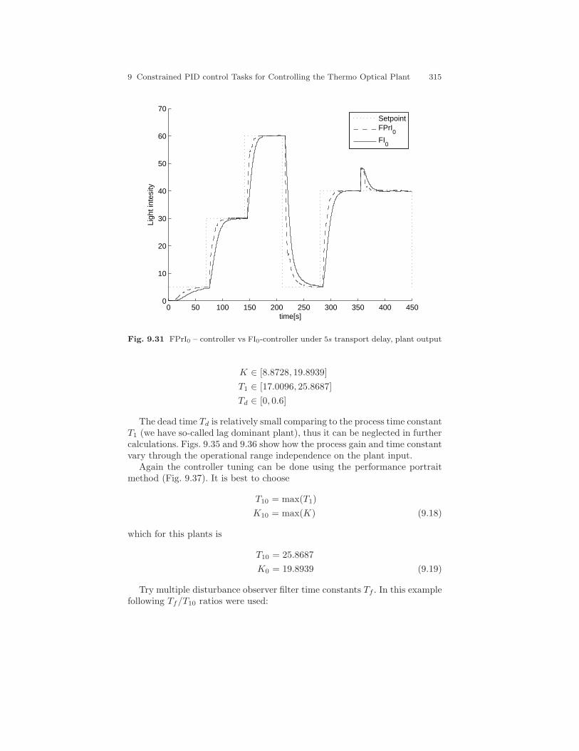
9 Constrained PID control Tasks for Controlling the Thermo Optical Plant 315
0 50 100 150 200 250 300 350 400 4500
10
20
30
40
50
60
70
time[s]
Ligh
t int
esity
SetpointFPrI
0FI
0
Fig. 9.31 FPrI0 – controller vs FI0-controller under 5s transport delay, plant output
K ∈ [8.8728, 19.8939]
T1 ∈ [17.0096, 25.8687]
Td ∈ [0, 0.6]
The dead time Td is relatively small comparing to the process time constantT1 (we have so-called lag dominant plant), thus it can be neglected in furthercalculations. Figs. 9.35 and 9.36 show how the process gain and time constantvary through the operational range independence on the plant input.
Again the controller tuning can be done using the performance portraitmethod (Fig. 9.37). It is best to choose
T10 = max(T1)
K10 = max(K) (9.18)
which for this plants is
T10 = 25.8687
K0 = 19.8939 (9.19)
Try multiple disturbance observer filter time constants Tf . In this examplefollowing Tf/T10 ratios were used:
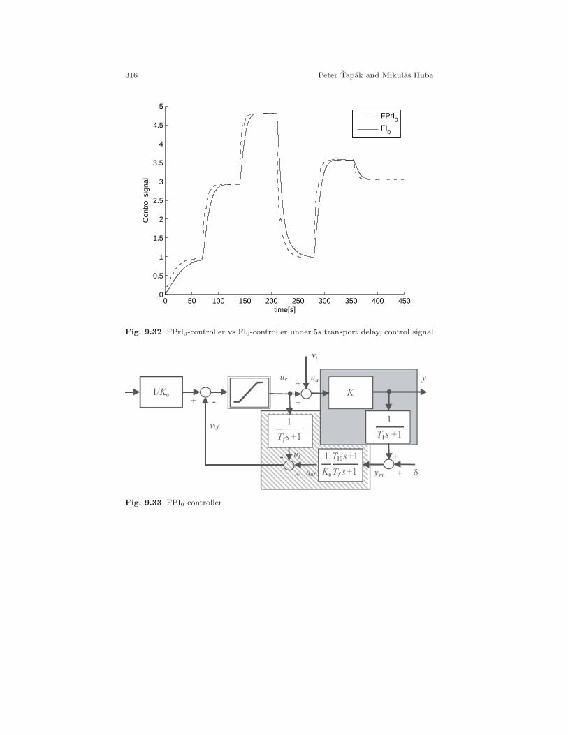
316 Peter Tapak and Mikulas Huba
0 50 100 150 200 250 300 350 400 4500
0.5
1
1.5
2
2.5
3
3.5
4
4.5
5
time[s]
Con
trol
sig
nal
FPrI
0
FI0
Fig. 9.32 FPrI0-controller vs FI0-controller under 5s transport delay, control signal
Fig. 9.33 FPI0 controller
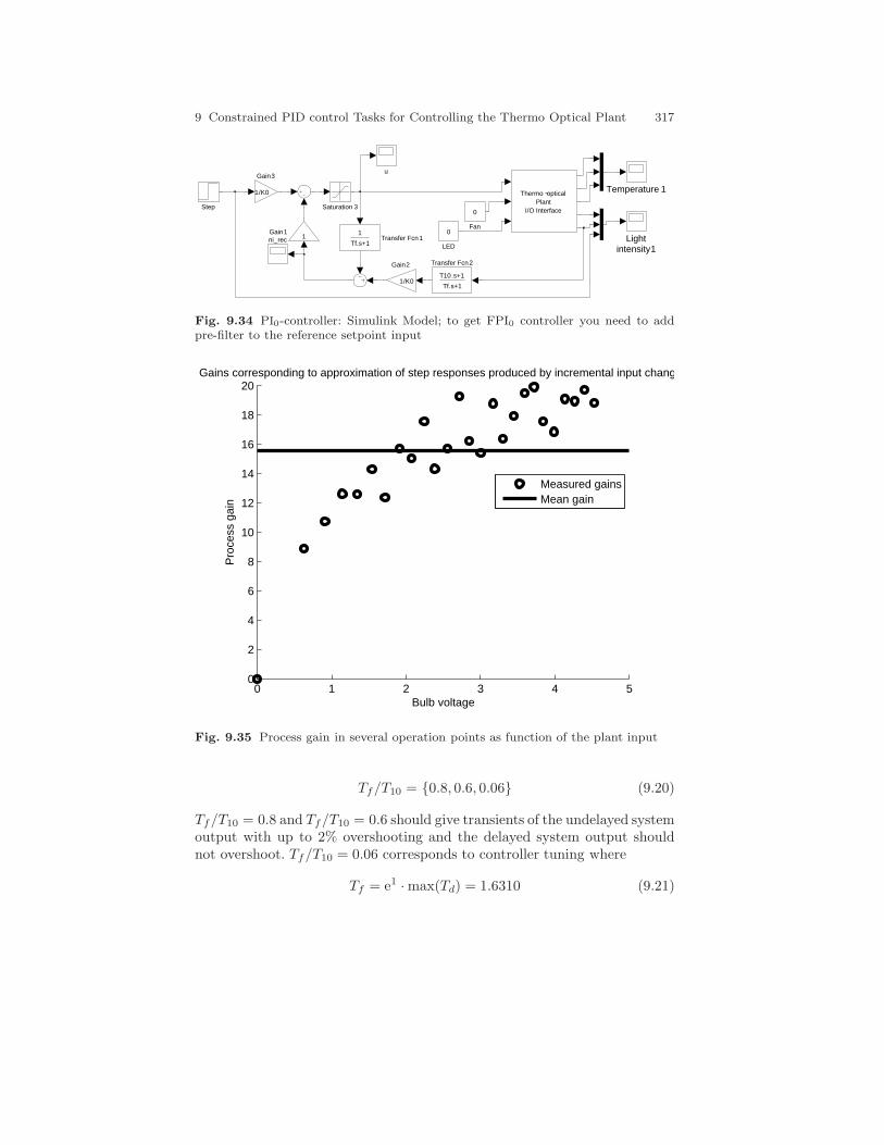
9 Constrained PID control Tasks for Controlling the Thermo Optical Plant 317
u
ni_rec
Transfer Fcn2
T10.s+1
Tf.s+1
Transfer Fcn11
Tf.s+1
Thermo −opticalPlant
I/O Interface
Temperature 1
Step Saturation 3
Lightintensity1LED
0
Gain3
1/K0
Gain2
1/K0
Gain11
Fan
0
Fig. 9.34 PI0-controller: Simulink Model; to get FPI0 controller you need to addpre-filter to the reference setpoint input
0 1 2 3 4 50
2
4
6
8
10
12
14
16
18
20Gains corresponding to approximation of step responses produced by incremental input changes
Bulb voltage
Pro
cess
gai
n
Measured gainsMean gain
Fig. 9.35 Process gain in several operation points as function of the plant input
Tf/T10 = 0.8, 0.6, 0.06 (9.20)
Tf/T10 = 0.8 and Tf/T10 = 0.6 should give transients of the undelayed systemoutput with up to 2% overshooting and the delayed system output shouldnot overshoot. Tf/T10 = 0.06 corresponds to controller tuning where
Tf = e1 ·max(Td) = 1.6310 (9.21)
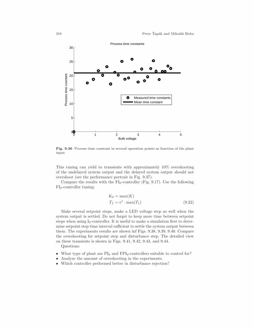
318 Peter Tapak and Mikulas Huba
0 1 2 3 4 50
5
10
15
20
25
30Process time constants
Bulb voltage
Pro
cess
tim
e co
snta
nt
Measured time constantsMean time constant
Fig. 9.36 Process time constant in several operation points as function of the plantinput
This tuning can yield to transients with approximately 10% overshootingof the undelayed system output and the delayed system output should notovershoot (see the performance portrait in Fig. 9.37).
Compare the results with the FI0-controller (Fig. 9.17). Use the followingFI0-controller tuning:
K0 = max(K)
Tf = e1 ·max(T1) (9.22)
Make several setpoint steps, make a LED voltage step as well when thesystem output is settled. Do not forget to keep more time between setpointsteps when using I0-controller. It is useful to make a simulation first to deter-mine setpoint step time interval sufficient to settle the system output betweenthem. The experiments results are shown inf Figs. 9.38, 9.39, 9.40. Comparethe overshooting for setpoint step and disturbance step. The detailed viewon these transients is shown in Figs. 9.41, 9.42, 9.43, and 9.44.
Questions:
• What type of plant are PI0 and FPI0-controllers suitable to control for?• Analyze the amount of overshooting in the experiments.• Which controller performed better in disturbance rejection?
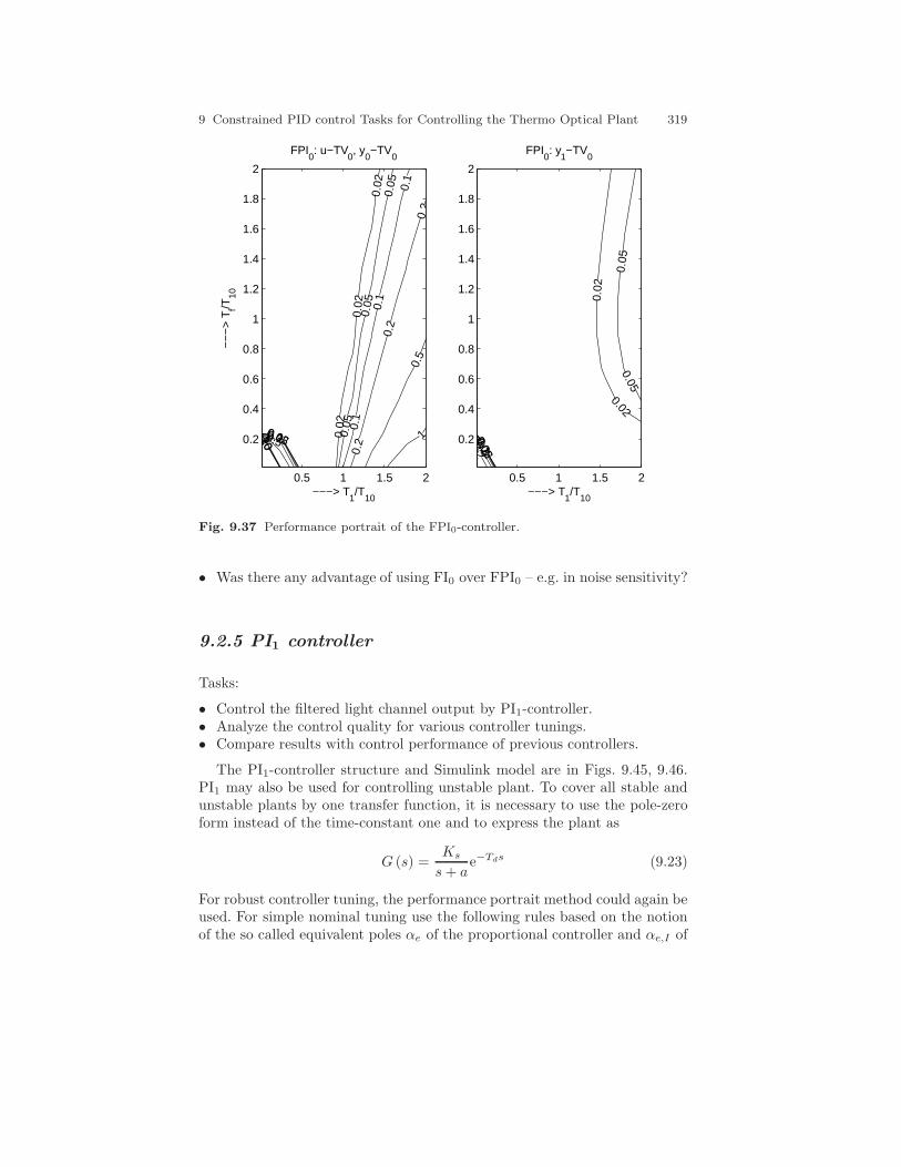
9 Constrained PID control Tasks for Controlling the Thermo Optical Plant 319
0.02 0.02
0.02
0.02
0.05 0.05
0.05
0.05
0.1
0.1
0.1
0.1
0.2
0.2
0.2
0.2
0.5
0.5
1 1251020
−−
−>
Tf/T
10
−−−> T1/T
10
FPI0: u−TV
0, y
0−TV
0
0.5 1 1.5 2
0.2
0.4
0.6
0.8
1
1.2
1.4
1.6
1.8
2
0.02
0.02
0.02
0.05
0.05
0.05
0.10.20.51
2
−−−> T1/T
10
FPI0: y
1−TV
0
0.5 1 1.5 2
0.2
0.4
0.6
0.8
1
1.2
1.4
1.6
1.8
2
Fig. 9.37 Performance portrait of the FPI0-controller.
• Was there any advantage of using FI0 over FPI0 – e.g. in noise sensitivity?
9.2.5 PI1 controller
Tasks:
• Control the filtered light channel output by PI1-controller.• Analyze the control quality for various controller tunings.• Compare results with control performance of previous controllers.
The PI1-controller structure and Simulink model are in Figs. 9.45, 9.46.PI1 may also be used for controlling unstable plant. To cover all stable andunstable plants by one transfer function, it is necessary to use the pole-zeroform instead of the time-constant one and to express the plant as
G (s) =Ks
s+ ae−Tds (9.23)
For robust controller tuning, the performance portrait method could again beused. For simple nominal tuning use the following rules based on the notionof the so called equivalent poles αe of the proportional controller and αe,I of
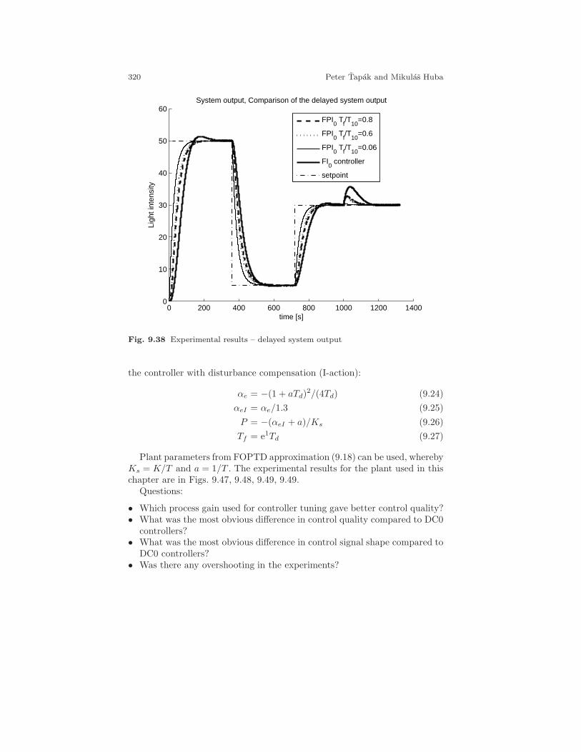
320 Peter Tapak and Mikulas Huba
0 200 400 600 800 1000 1200 14000
10
20
30
40
50
60
time [s]
Ligh
t int
ensi
ty
System output, Comparison of the delayed system output
FPI
0 T
f/T
10=0.8
FPI0 T
f/T
10=0.6
FPI0 T
f/T
10=0.06
FI0 controller
setpoint
Fig. 9.38 Experimental results – delayed system output
the controller with disturbance compensation (I-action):
αe = −(1 + aTd)2/(4Td) (9.24)
αeI = αe/1.3 (9.25)
P = −(αeI + a)/Ks (9.26)
Tf = e1Td (9.27)
Plant parameters from FOPTD approximation (9.18) can be used, wherebyKs = K/T and a = 1/T . The experimental results for the plant used in thischapter are in Figs. 9.47, 9.48, 9.49, 9.49.
Questions:
• Which process gain used for controller tuning gave better control quality?• What was the most obvious difference in control quality compared to DC0
controllers?• What was the most obvious difference in control signal shape compared to
DC0 controllers?• Was there any overshooting in the experiments?
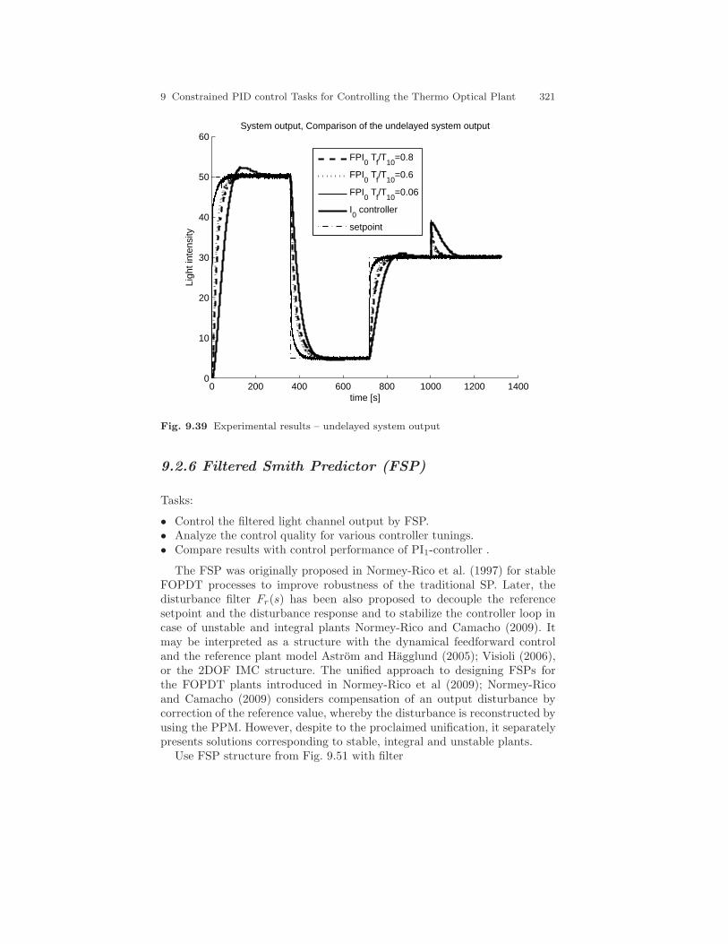
9 Constrained PID control Tasks for Controlling the Thermo Optical Plant 321
0 200 400 600 800 1000 1200 14000
10
20
30
40
50
60
time [s]
Ligh
t int
ensi
ty
System output, Comparison of the undelayed system output
FPI0 T
f/T
10=0.8
FPI0 T
f/T
10=0.6
FPI0 T
f/T
10=0.06
I0 controller
setpoint
Fig. 9.39 Experimental results – undelayed system output
9.2.6 Filtered Smith Predictor (FSP)
Tasks:
• Control the filtered light channel output by FSP.• Analyze the control quality for various controller tunings.• Compare results with control performance of PI1-controller .
The FSP was originally proposed in Normey-Rico et al. (1997) for stableFOPDT processes to improve robustness of the traditional SP. Later, thedisturbance filter Fr(s) has been also proposed to decouple the referencesetpoint and the disturbance response and to stabilize the controller loop incase of unstable and integral plants Normey-Rico and Camacho (2009). Itmay be interpreted as a structure with the dynamical feedforward controland the reference plant model Astrom and Hagglund (2005); Visioli (2006),or the 2DOF IMC structure. The unified approach to designing FSPs forthe FOPDT plants introduced in Normey-Rico et al (2009); Normey-Ricoand Camacho (2009) considers compensation of an output disturbance bycorrection of the reference value, whereby the disturbance is reconstructed byusing the PPM. However, despite to the proclaimed unification, it separatelypresents solutions corresponding to stable, integral and unstable plants.
Use FSP structure from Fig. 9.51 with filter
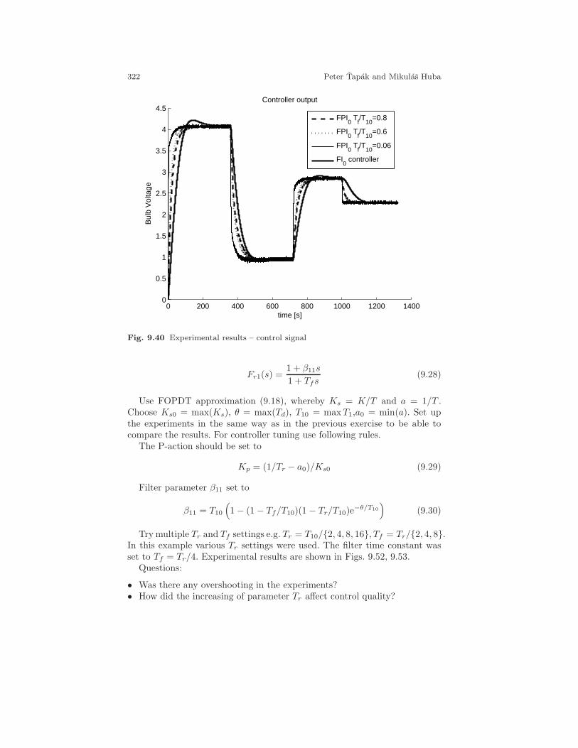
322 Peter Tapak and Mikulas Huba
0 200 400 600 800 1000 1200 14000
0.5
1
1.5
2
2.5
3
3.5
4
4.5
time [s]
Bul
b V
olta
ge
Controller output
FPI
0 T
f/T
10=0.8
FPI0 T
f/T
10=0.6
FPI0 T
f/T
10=0.06
FI0 controller
Fig. 9.40 Experimental results – control signal
Fr1(s) =1 + β11s
1 + Tfs(9.28)
Use FOPDT approximation (9.18), whereby Ks = K/T and a = 1/T .Choose Ks0 = max(Ks), θ = max(Td), T10 = maxT1,a0 = min(a). Set upthe experiments in the same way as in the previous exercise to be able tocompare the results. For controller tuning use following rules.
The P-action should be set to
Kp = (1/Tr − a0)/Ks0 (9.29)
Filter parameter β11 set to
β11 = T10
(1− (1 − Tf/T10)(1 − Tr/T10)e
−θ/T10
)(9.30)
Try multiple Tr and Tf settings e.g. Tr = T10/2, 4, 8, 16,Tf = Tr/2, 4, 8.In this example various Tr settings were used. The filter time constant wasset to Tf = Tr/4. Experimental results are shown in Figs. 9.52, 9.53.
Questions:
• Was there any overshooting in the experiments?• How did the increasing of parameter Tr affect control quality?
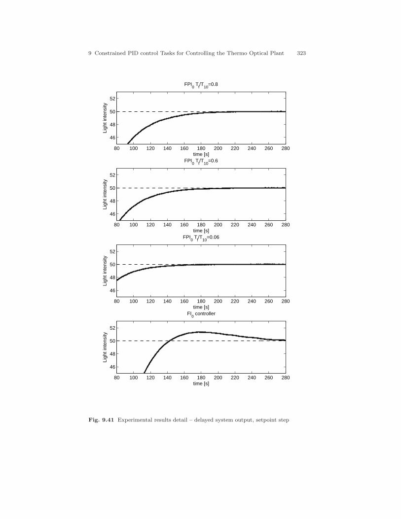
9 Constrained PID control Tasks for Controlling the Thermo Optical Plant 323
80 100 120 140 160 180 200 220 240 260 280
46
48
50
52Li
ght i
nten
sity
time [s]
FPI0 T
f/T
10=0.8
80 100 120 140 160 180 200 220 240 260 280
46
48
50
52
Ligh
t int
ensi
ty
time [s]
FPI0 T
f/T
10=0.6
80 100 120 140 160 180 200 220 240 260 280
46
48
50
52
Ligh
t int
ensi
ty
time [s]
FPI0 T
f/T
10=0.06
80 100 120 140 160 180 200 220 240 260 280
46
48
50
52
Ligh
t int
ensi
ty
time [s]
FI0 controller
Fig. 9.41 Experimental results detail – delayed system output, setpoint step
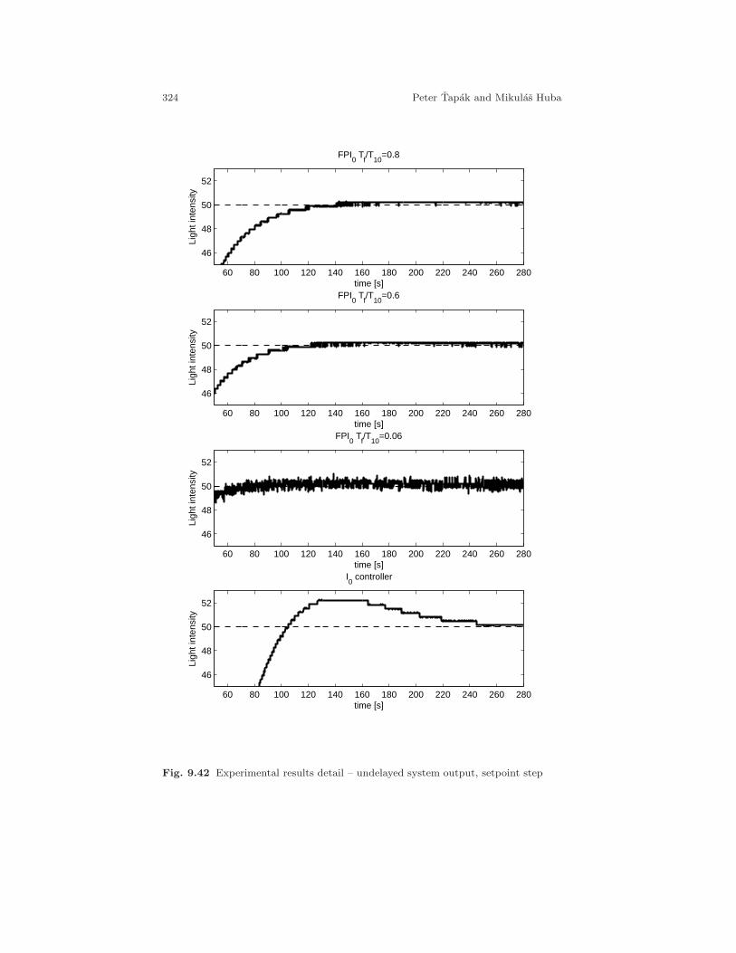
324 Peter Tapak and Mikulas Huba
60 80 100 120 140 160 180 200 220 240 260 280
46
48
50
52Li
ght i
nten
sity
time [s]
FPI0 T
f/T
10=0.8
60 80 100 120 140 160 180 200 220 240 260 280
46
48
50
52
Ligh
t int
ensi
ty
time [s]
FPI0 T
f/T
10=0.6
60 80 100 120 140 160 180 200 220 240 260 280
46
48
50
52
Ligh
t int
ensi
ty
time [s]
FPI0 T
f/T
10=0.06
60 80 100 120 140 160 180 200 220 240 260 280
46
48
50
52
Ligh
t int
ensi
ty
time [s]
I0 controller
Fig. 9.42 Experimental results detail – undelayed system output, setpoint step
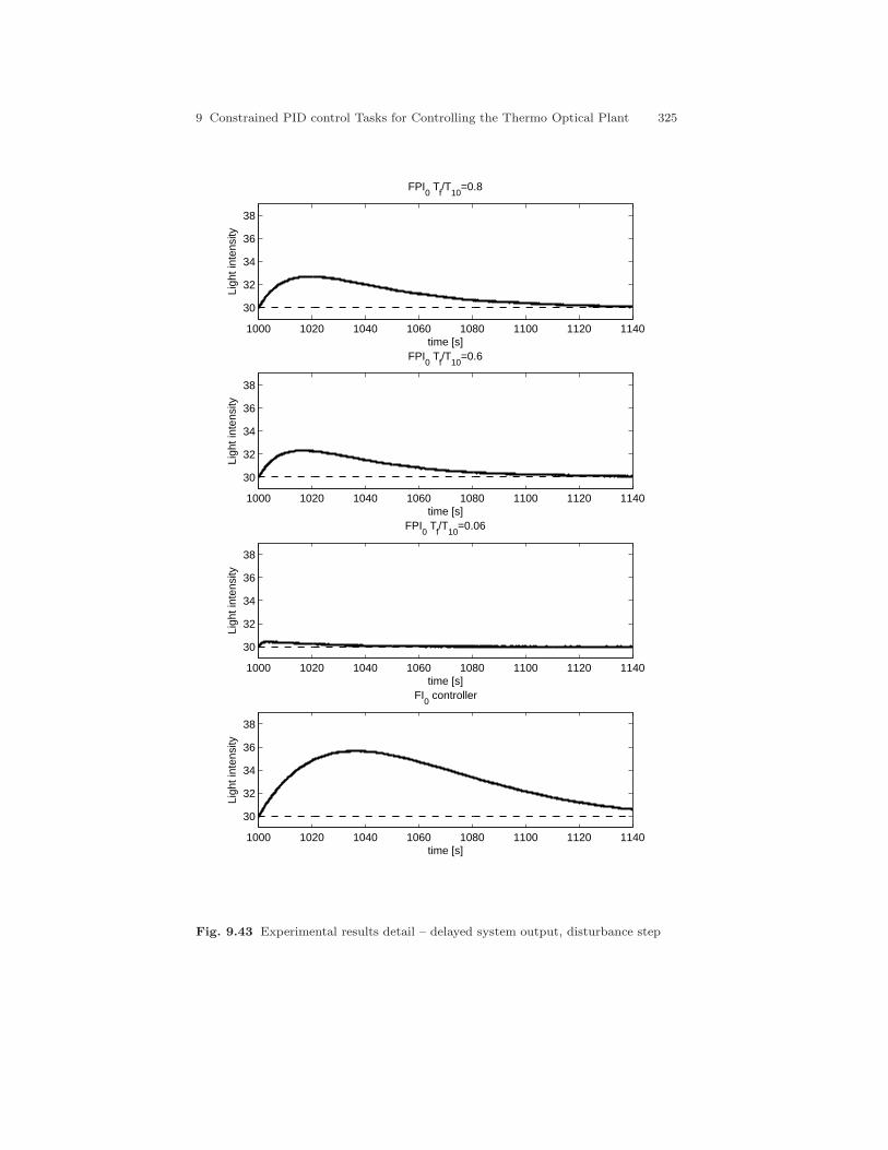
9 Constrained PID control Tasks for Controlling the Thermo Optical Plant 325
1000 1020 1040 1060 1080 1100 1120 1140
30
32
34
36
38Li
ght i
nten
sity
time [s]
FPI0 T
f/T
10=0.8
1000 1020 1040 1060 1080 1100 1120 1140
30
32
34
36
38
Ligh
t int
ensi
ty
time [s]
FPI0 T
f/T
10=0.6
1000 1020 1040 1060 1080 1100 1120 1140
30
32
34
36
38
Ligh
t int
ensi
ty
time [s]
FPI0 T
f/T
10=0.06
1000 1020 1040 1060 1080 1100 1120 1140
30
32
34
36
38
Ligh
t int
ensi
ty
time [s]
FI0 controller
Fig. 9.43 Experimental results detail – delayed system output, disturbance step
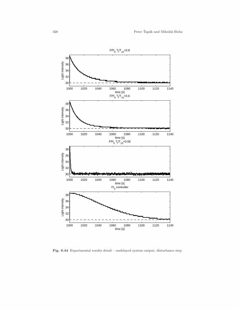
326 Peter Tapak and Mikulas Huba
1000 1020 1040 1060 1080 1100 1120 1140
30
32
34
36
38Li
ght i
nten
sity
time [s]
FPI0 T
f/T
10=0.8
1000 1020 1040 1060 1080 1100 1120 1140
30
32
34
36
38
Ligh
t int
ensi
ty
time [s]
FPI0 T
f/T
10=0.6
1000 1020 1040 1060 1080 1100 1120 1140
30
32
34
36
38
Ligh
t int
ensi
ty
time [s]
FPI0 T
f/T
10=0.06
1000 1020 1040 1060 1080 1100 1120 1140
30
32
34
36
38
Ligh
t int
ensi
ty
time [s]
FI0 controller
Fig. 9.44 Experimental results detail – undelayed system output, disturbance step
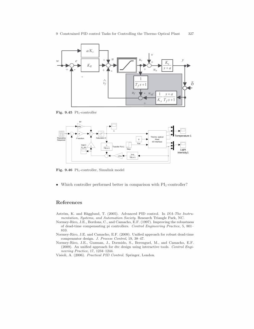
9 Constrained PID control Tasks for Controlling the Thermo Optical Plant 327
KR
-
-
-
+
+
+++
v
ur y
uf
ua
vf
ew
a/Ks
u
^
afu
d1
1
+sT f
1
1
+
+
sT
as
K fs
as
Ks
+
+
-
Fig. 9.45 PI1-controller
u
ni_rec
s+a
Tfil.s+1
Transfer Fcn11
Tfil.s+1
Thermo −opticalPlant
I/O Interface
Temperature 1
Step
Saturation 3RepeatingSequence
P−asction
P
Lightintensity1
1/Ks
Gain11
Fan
0
FF
a/Ks
Fig. 9.46 PI1-controller, Simulink model
• Which controller performed better in comparison with PI1-controller?
References
Astrom, K. and Hagglund, T. (2005). Advanced PID control. In ISA-The Instru-
mentation, Systems, and Automation Society. Research Triangle Park, NC.Normey-Rico, J.E., Bordons, C., and Camacho, E.F. (1997). Improving the robustness
of dead-time compensating pi controllers. Control Engineering Practice, 5, 801–810.
Normey-Rico, J.E. and Camacho, E.F. (2009). Unified approach for robust dead-timecompensator design. J. Process Control, 19, 38–47.
Normey-Rico, J.E., Guzman, J., Dormido, S., Berenguel, M., and Camacho, E.F.(2009). An unified approach for dtc design using interactive tools. Control Engi-
neering Practice, 17, 1234–1244.Visioli, A. (2006). Practical PID Control. Springer, London.

328 Peter Tapak and Mikulas Huba
0 20 40 60 80 1000
10
20
30
40
50
60
70
time [s]
Ligh
t int
ensi
ty
PI1 controller − output of filtered light channel, K=19
delayed outputundelayed outputsetpoint
Fig. 9.47 PI1-controller, filtered light channel control for K = 19
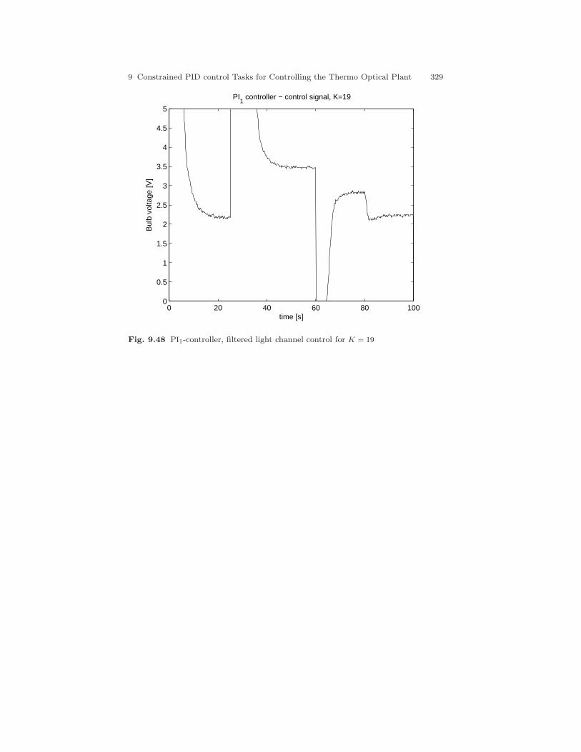
9 Constrained PID control Tasks for Controlling the Thermo Optical Plant 329
0 20 40 60 80 1000
0.5
1
1.5
2
2.5
3
3.5
4
4.5
5
time [s]
Bul
b vo
ltage
[V]
PI1 controller − control signal, K=19
Fig. 9.48 PI1-controller, filtered light channel control for K = 19
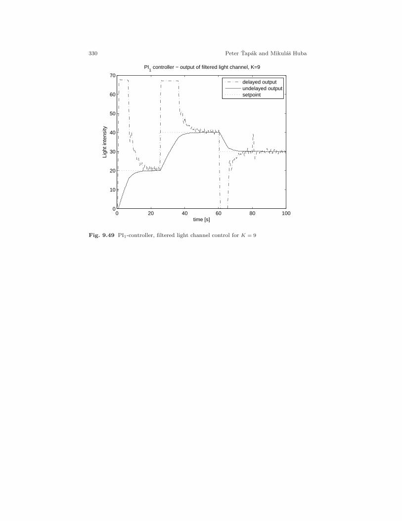
330 Peter Tapak and Mikulas Huba
0 20 40 60 80 1000
10
20
30
40
50
60
70
time [s]
Ligh
t int
ensi
ty
PI1 controller − output of filtered light channel, K=9
delayed outputundelayed outputsetpoint
Fig. 9.49 PI1-controller, filtered light channel control for K = 9
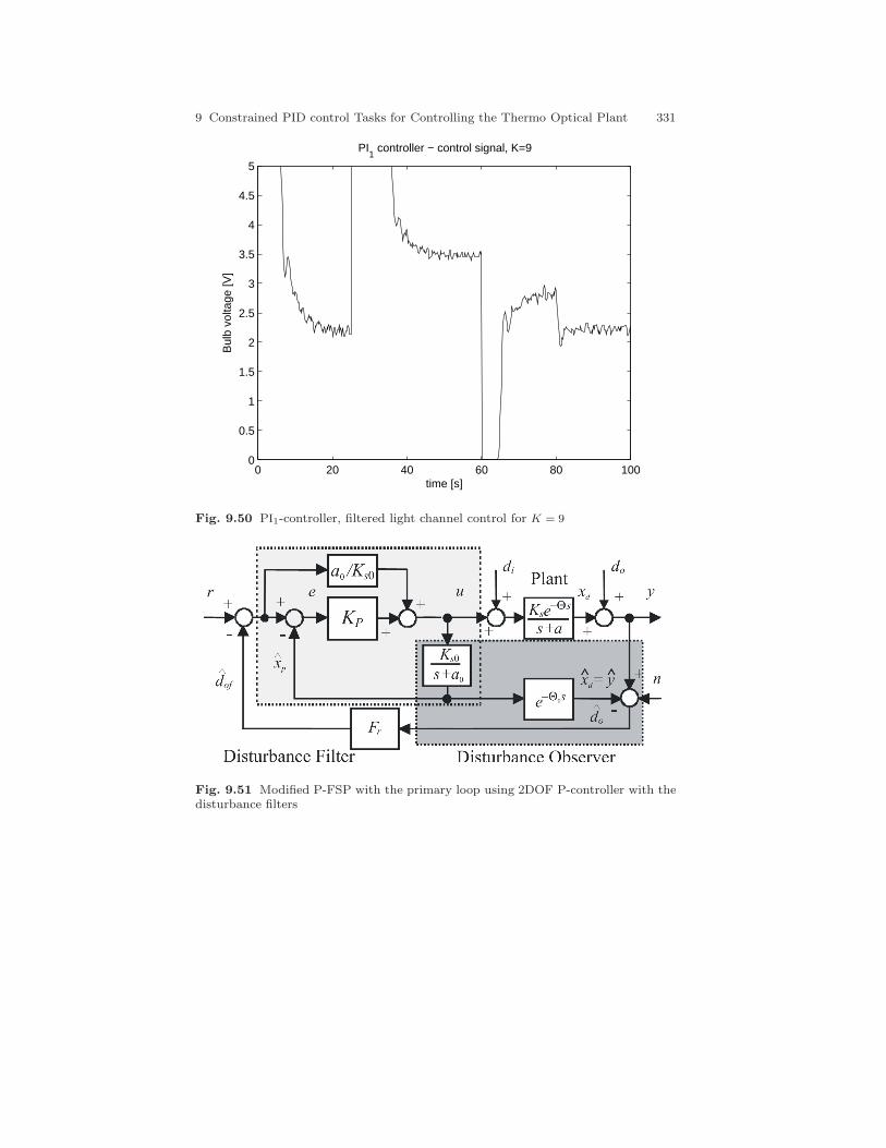
9 Constrained PID control Tasks for Controlling the Thermo Optical Plant 331
0 20 40 60 80 1000
0.5
1
1.5
2
2.5
3
3.5
4
4.5
5
time [s]
Bul
b vo
ltage
[V]
PI1 controller − control signal, K=9
Fig. 9.50 PI1-controller, filtered light channel control for K = 9
Fig. 9.51 Modified P-FSP with the primary loop using 2DOF P-controller with thedisturbance filters
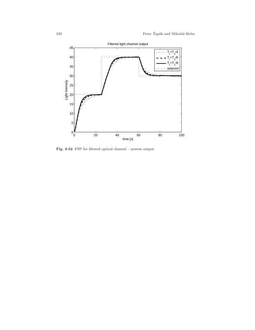
332 Peter Tapak and Mikulas Huba
0 20 40 60 80 1000
5
10
15
20
25
30
35
40
45
time [s]
Ligh
t int
ensi
ty
Filtered light channel output
T
r=T
1/4
Tr=T
1/6
Tr=T
1/8
setpoint
Fig. 9.52 FSP for filtered optical channel – system output
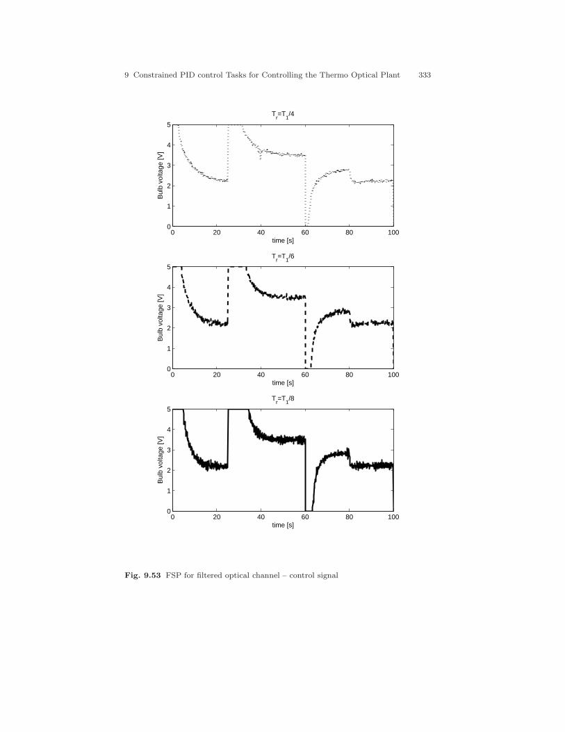
9 Constrained PID control Tasks for Controlling the Thermo Optical Plant 333
0 20 40 60 80 1000
1
2
3
4
5
Tr=T
1/4
time [s]
Bul
b vo
ltage
[V]
0 20 40 60 80 1000
1
2
3
4
5
time [s]
Bul
b vo
ltage
[V]
Tr=T
1/6
0 20 40 60 80 1000
1
2
3
4
5
Tr=T
1/8
time [s]
Bul
b vo
ltage
[V]
Fig. 9.53 FSP for filtered optical channel – control signal

334 Peter Tapak and Mikulas Huba
Comments – Remarks

9 Constrained PID control Tasks for Controlling the Thermo Optical Plant 335
Comments – Remarks

336 Peter Tapak and Mikulas Huba
Comments – Remarks

9 Constrained PID control Tasks for Controlling the Thermo Optical Plant 337
Comments – Remarks
