Seismic Records of the 2004 Sumatra and Other Tsunamis:

A Quantitative Study

EMILE A. OKAL

Abstract—Following the recent reports by YUAN et al. (2005) of recordings of the 2004 Sumatra

tsunami on the horizontal components of coastal seismometers in the Indian Ocean basin, we build a much

enhanced dataset extending into the Atlantic and Pacific Oceans, as far away as Bermuda and Hawaii, and

also expanded to five additional events in the years 1995–2006. In order to interpret these records

quantitatively, we propose that the instruments are responding to the combination of horizontal

displacement, tilt and perturbation in gravity described by GILBERT (1980), and induced by the passage of

the progressive tsunami wave over the ocean basin. In this crude approximation, we simply ignore the

island or continent structure, and assume that the seismometer functions de facto as an ocean-bottom

instrument. The records can then be interpreted in the framework of tsunami normal mode theory,and lead

to acceptable estimates of the seismic moment of the parent earthquakes. We further demonstrate the

feasibility of deconvolving the response of the ocean floor in order to reconstruct the time series of the

tsunami wave height at the surface of the ocean, suggesting that island or coastal continental seismometers

could complement the function of tsunameters.

Key words: Tsunami, seismic recording, 2004 Sumatra earthquake.

Introduction

In the aftermath of the 2004 Sumatra tsunami, YUAN et al. (2005) reported that

seven seismic stations located on islands and continental shores of the Indian Ocean

had recorded on their horizontal components the actual impact of the tsunami on the

nearby shores. These signals were generally polarized perpendicular to the shoreline

and featured energy in the 1 to 2 mHz range and amplitudes, expressed as

accelerations, on the order of 10)4 cm/s2. Following the landslides at Stromboli in

2002, LA ROCCA et al. (2004) had similarly reported low-frequency signals at the

seismic station on the nearby island of Panarea (21 km away from the source), but

Yuan et al.’s remarkable observations constitute the first such report in the far field.

They were also briefly confirmed by HANSON and BOWMAN (2005).

Department of Geological Sciences, Northwestern University, Evanston, IL 60201, USA.

Pure appl. geophys. 164 (2007) 325–3530033–4553/07/030325–29DOI 10.1007/s00024-006-0181-4

� Birkhauser Verlag, Basel, 2007

Pure and Applied Geophysics

In this context, the purpose of the present paper is to expand on YUAN et al.’s

(2005) work in several directions, by showing that such recordings were detectable

worldwide; that the signals extend, at least in the regional field, to high frequencies

in the 10 mHz range; that such signals are justifiable quantitatively using normal

mode theory; that similar signals from smaller tsunamis are also identifiable in the

seismic record, with their spectral amplitudes correlating well with the seismic

moment of the parent earthquake; that acceptable time series of the tsunami on the

high seas can be reconstructed from seismic records; and finally that seismic records

of tsunami waves can also be obtained on vertical seismometers, albeit at a lower

amplitude.

2. The Universal Character of the Seismic Recordings

Following in the footsteps of YUAN et al. (2005), we conducted a systematic

worldwide search for similar records, including at stations located outside the

Indian Ocean. At each targeted station, we extracted the long-period horizontal

channels, and proceeded to deconvolve the instrument and bandpass filter the

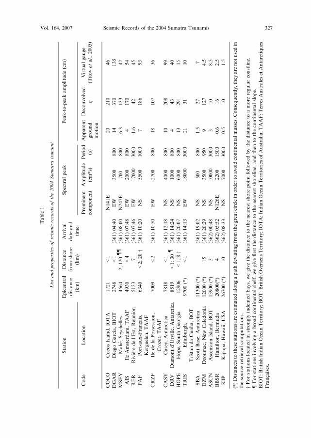
resulting ground motion between 0.1 and 10 mHz. Table 1 lists the stations at

which the tsunami was detected, with relevant information such as dominant

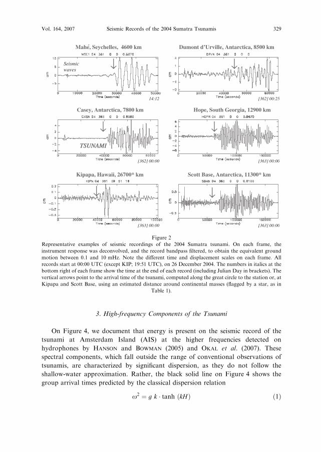
frequency and equivalent amplitude; their location is shown on Figure 1. Figure 2

provides representative examples of typical time series, after deconvolution of the

instrument response to ground displacement and bandpass filtering in the

0.1–10 mHz range. The association of the signals with the tsunami was made on

the basis of its arrival time, as predicted by the global simulation of TITOV et al.

(2005). Among the most remarkable results, we note that the tsunami is well

recorded seismically as far as Bermuda (29 hours after origin time and at a distance

of 20,800 km around the Cape of Good Hope), and Kipapa, Hawaii (31.5 hours

after origin time). The latter site is reached after a westward path estimated at

26,700 km, through the Atlantic Ocean and the Drake Passage (the eastward path

going south of Australia being about 8 hours shorter). This is an expression of the

strong directivity of the source towards the Western Indian Ocean, at right angles

to the direction of faulting (BEN-MENAHEM and ROSENMAN, 1972), and of the

efficient focusing of the wave by the shallow bathymetry along the Southwest

Indian Ridge (TITOV et al., 2005) as previously observed for Pacific Ocean tsunamis

by WOODS and OKAL (1987) and SATAKE (1988). These effects also probably

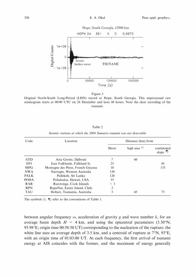
contribute to the spectacular quality of the recording at Hope, South Georgia,

where the tsunami is clearly discernible on the raw record, without the need for

filtering or instrument deconvolution (Fig. 3); they may be compounded by local

resonance effects in the Bays of Cumberland. The tsunami is also well recorded at

station SBA (Scott Base, Antarctica), following a somewhat convoluted path

around Australia and into McMurdo Sound.

326 E. A. Okal Pure appl. geophys.,

Table

1

Listandproperties

ofseismic

recordsofthe2004Sumatratsunami

Station

Epicentral

distance

(km)

Distance

from

shore

(km)

Arrival

date

and

time

Spectralpeak

Peak-to-peakamplitude(cm)

Code

Location

Prominent

component

Amplitude

(cm*s)

Period

(s)

Apparent

ground

motion

Deconvolved

gVirtualgauge

(Titovet

al.,2005)

COCO

CocosIsland,IO

TA

1721

<1

N141E

20

210

46

DGAR

DiegoGarcia,BIO

T2748

<1

(361)04:40

EW

3500

800

14

370

135

MSEY

Mahe,

Seychelles

4564

2;120{{

(361)08:00

N247E

700

800

6.3

133

42

AIS

IleAmsterdam,TAAF

4930

<4

(361)07:48

EW

2000

800

4170

54

RER

Riviere

del’Est,Reunion

5133

7(361)07:46

EW

17000

3000

1.6

42

45

PAF

Port-aux-Francais,

Kerguelen,TAAF

6340

<2;20y

(361)10:20

NS

5500

1000

7186

93

CRZF

Iledela

Possession,

Crozet,TAAF

7009

<2

(361)10:50

EW

2700

800

18

107

36

CASY

Casey,Antarctica

7818

<1

(361)12:18

NS

4000

800

10

208

99

DRV

Dumontd’U

rville,Antarctica

8519

<1;30{

(361)14:24

NS

1000

800

443

40

HOPE

Hope,

South

Georgia

12906

<1;8y

(361)20:07

NS

6000

800

13

291

15

TRIS

Edinburgh,

TristandaCunha,BOT

9700(*)

<1

(361)14:13

EW

18000

3000

21

31

10

SBA

ScottBase,Antarctica

11300(*)

(361)19:02

NS

500

800

1.5

27

7

DZM

Dzoumac,

New

Caledonia

12000(*)

15

(361)20:29

NS

3500

950

9127

4.5

ASCN

AscensionIsland,BOT

13900(*)

3(362)00:48

NS

10000

3000

310

8.5

BBSR

Hamilton,Bermuda

20800(*)

4(362)05:52

N126E

2200

1500

0.6

16

2.5

KIP

Kipapa,Hawaii,USA

26700(*)

10

(362)08:33

NS

7000

3000

0.5

10

1.5

(*)Distancesto

thesestationsare

estimatedalongapath

deviatingfrom

thegreatcirclein

order

toavoid

continentalmasses.Consequently,they

are

notusedin

thesourceretrievalcomputations.

yForstationslocatedin

strongly

indentedbays,wegivethedistance

tothenearest

shore

pointfollowed

bythedistance

toamore

regularcoastline.

{Forstationsinvolvingabroadcontinentalshelf,wegivefirstthedistance

tothenearest

shoreline,

andthen

tothecontinentalslope.

BIO

T:British

IndianOceanTerritory;BOT:British

OverseasTerritory;IO

TA:IndianOceanTerritories

ofAustralia;TAAF:TerresAustraleset

Antarctiques

Francaises.

Vol. 164, 2007 Seismic Records of the 2004 Sumatra Tsunamis 327

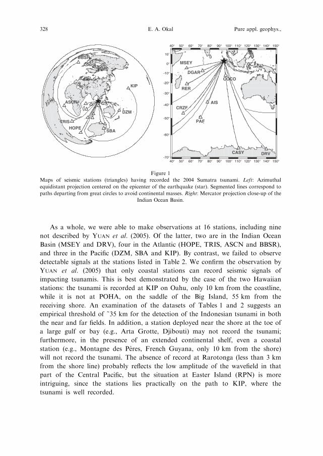
As a whole, we were able to make observations at 16 stations, including nine

not described by YUAN et al. (2005). Of the latter, two are in the Indian Ocean

Basin (MSEY and DRV), four in the Atlantic (HOPE, TRIS, ASCN and BBSR),

and three in the Pacific (DZM, SBA and KIP). By contrast, we failed to observe

detectable signals at the stations listed in Table 2. We confirm the observation by

YUAN et al. (2005) that only coastal stations can record seismic signals of

impacting tsunamis. This is best demonstrated by the case of the two Hawaiian

stations: the tsunami is recorded at KIP on Oahu, only 10 km from the coastline,

while it is not at POHA, on the saddle of the Big Island, 55 km from the

receiving shore. An examination of the datasets of Tables 1 and 2 suggests an

empirical threshold of ~35 km for the detection of the Indonesian tsunami in both

the near and far fields. In addition, a station deployed near the shore at the toe of

a large gulf or bay (e.g., Arta Grotte, Djibouti) may not record the tsunami;

furthermore, in the presence of an extended continental shelf, even a coastal

station (e.g., Montagne des Peres, French Guyana, only 10 km from the shore)

will not record the tsunami. The absence of record at Rarotonga (less than 3 km

from the shore line) probably reflects the low amplitude of the wavefield in that

part of the Central Pacific, but the situation at Easter Island (RPN) is more

intriguing, since the stations lies practically on the path to KIP, where the

tsunami is well recorded.

KIP

BBSR

HOPETRIS

ASCN

SBA

DZM

40°

40°

50°

50°

60°

60°

70°

70°

80°

80°

90°

90°

100°

100°

110°

110°

120°

120°

130°

130°

140°

140°

150°

150°

-70°

-60°

-50°

-40°

-30°

-20°

-10°

0°

10˚

MSEY

RER

CRZF

PAF

AIS

DGAR

COCO

CASY DRV

Figure 1

Maps of seismic stations (triangles) having recorded the 2004 Sumatra tsunami. Left: Azimuthal

equidistant projection centered on the epicenter of the earthquake (star). Segmented lines correspond to

paths departing from great circles to avoid continental masses. Right: Mercator projection close-up of the

Indian Ocean Basin.

328 E. A. Okal Pure appl. geophys.,

3. High-frequency Components of the Tsunami

On Figure 4, we document that energy is present on the seismic record of the

tsunami at Amsterdam Island (AIS) at the higher frequencies detected on

hydrophones by HANSON and BOWMAN (2005) and OKAL et al. (2007). These

spectral components, which fall outside the range of conventional observations of

tsunamis, are characterized by significant dispersion, as they do not follow the

shallow-water approximation. Rather, the black solid line on Figure 4 shows the

group arrival times predicted by the classical dispersion relation

x2 ¼ g k � tanh ðkHÞ ð1Þ

.≈

Casey, Antarctica, 7800 km Hope, South Georgia, 12900 km

Kipapa, Hawaii, 26700* km Scott Base, Antarctica, 11300* km

TSUNAMITSUNAMI

↓

↓↓

↓ ↓

↓

Mahe, Seychelles, 4600 km Dumont d’Urville, Antarctica, 8500 km

Seismicwaves

14:12

[362] 00:00

[363] 00:00

[362] 00:25

[363] 00:00

[363] 00:00

´

Figure 2

Representative examples of seismic recordings of the 2004 Sumatra tsunami. On each frame, the

instrument response was deconvolved, and the record bandpass filtered, to obtain the equivalent ground

motion between 0.1 and 10 mHz. Note the different time and displacement scales on each frame. All

records start at 00:00 UTC (except KIP; 19:51 UTC), on 26 December 2004. The numbers in italics at the

bottom right of each frame show the time at the end of each record (including Julian Day in brackets). The

vertical arrows point to the arrival time of the tsunami, computed along the great circle to the station or, at

Kipapa and Scott Base, using an estimated distance around continental masses (flagged by a star, as in

Table 1).

Vol. 164, 2007 Seismic Records of the 2004 Sumatra Tsunamis 329

between angular frequency x, acceleration of gravity g and wave number k, for an

average basin depth H = 4 km, and using the epicentral parameters (3.30�N;

95.98�E; origin time 00:58:50 UT) corresponding to the nucleation of the rupture; the

white line uses an average depth of 3.5 km, and a centroid of rupture at 7�N, 93�E,with an origin time of 01:03:00 UT. At each frequency, the first arrival of tsunami

energy at AIS coincides with the former, and the maximum of energy generally

Figure 3

Original North-South Long-Period (LHN) record at Hope, South Georgia. This unprocessed raw

seismogram starts at 00:00 UTC on 26 December and lasts 48 hours. Note the clear recording of the

tsunami.

Table 2

Seismic stations at which the 2004 Sumatra tsunami was not detectable

Code Location Distance (km) from

Shore high seas ðyÞ continental

slope ð{Þ

ATD Arta Grotte, Djibouti 7 60

EFI East Falklands, Falkland Is. 25 45

MPG Montagne des Peres, French Guyana 10 135

NWA Narrogin, Western Australia 150

PALK Pallekele, Sri Lanka 120

POHA Pohakuloa, Hawaii, USA 55

RAR Rarotonga, Cook Islands < 3

RPN RapaNui, Easter Island, Chile 3

TAU Hobart, Tasmania, Australia 3 45 75

The symbols ðy; {Þ refer to the conventions of Table 1.

330 E. A. Okal Pure appl. geophys.,

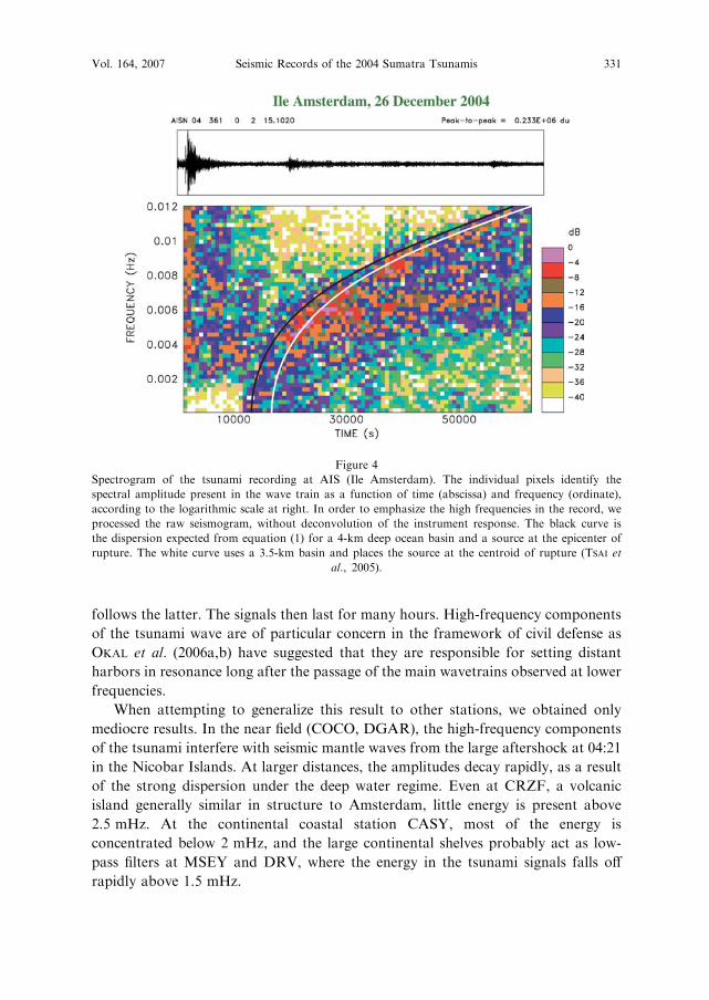
follows the latter. The signals then last for many hours. High-frequency components

of the tsunami wave are of particular concern in the framework of civil defense as

OKAL et al. (2006a,b) have suggested that they are responsible for setting distant

harbors in resonance long after the passage of the main wavetrains observed at lower

frequencies.

When attempting to generalize this result to other stations, we obtained only

mediocre results. In the near field (COCO, DGAR), the high-frequency components

of the tsunami interfere with seismic mantle waves from the large aftershock at 04:21

in the Nicobar Islands. At larger distances, the amplitudes decay rapidly, as a result

of the strong dispersion under the deep water regime. Even at CRZF, a volcanic

island generally similar in structure to Amsterdam, little energy is present above

2.5 mHz. At the continental coastal station CASY, most of the energy is

concentrated below 2 mHz, and the large continental shelves probably act as low-

pass filters at MSEY and DRV, where the energy in the tsunami signals falls off

rapidly above 1.5 mHz.

Figure 4

Spectrogram of the tsunami recording at AIS (Ile Amsterdam). The individual pixels identify the

spectral amplitude present in the wave train as a function of time (abscissa) and frequency (ordinate),

according to the logarithmic scale at right. In order to emphasize the high frequencies in the record, we

processed the raw seismogram, without deconvolution of the instrument response. The black curve is

the dispersion expected from equation (1) for a 4-km deep ocean basin and a source at the epicenter of

rupture. The white curve uses a 3.5-km basin and places the source at the centroid of rupture (TSAI et

al., 2005).

Vol. 164, 2007 Seismic Records of the 2004 Sumatra Tsunamis 331

4. Quantification of the Seismic Records of the Tsunami

In order to interpret the seismic records of the tsunami, we concentrate on their

low-frequency components, typically in the 0.3–1.5 mHz range, and note that at such

periods, the receiving stations are generally within one wavelength of the abyssal

plain where most of the propagation takes place. We then make the extreme

simplifying assumption that the shoreline seismometer actually functions as a

horizontal Ocean-Bottom Seismometer (OBS), simply attached to the solid Earth

structure underlying the water column in an unperturbed abyssal plain. Following

the seminal work of WARD (1980), it has long been known that the tsunami

eigenfunction is not limited to the oceanic layer, but is prolonged into any

substratum with finite rigidity l in the form of a pseudo-Rayleigh wave in which

potential energy is mostly elastic, as opposed to gravitational in the fluid (OKAL,

2003). While boundary conditions predict a discontinuity of the horizontal

component of particle displacement at the ocean bottom, the latter does not vanish

in the elastic medium, where its expression can be obtained in the limit x fi 0 as

l y3 ¼1

4� gqwg

lkð2Þ

using the formalism of OKAL (1988, 1991, 2003) and the notation of SAITO (1967); g is

the vertical amplitude of the eigenfunction y1 at the surface of the ocean, and qw the

density of the ocean water.

In addition, we note following GILBERT (1980) that a horizontal seismometer

responds to a spheroidal mode of the Earth through the combination of its

horizontal displacement, of the tilt component of the strain induced by the passage of

the equivalent wave, and of a component of gravity anomaly. As fully discussed in

the Appendix, the effect of the latter two is usually negligible, at most marginal, for

seismic modes, but will become primordial for a tsunami mode.

We rewrite GILBERT’s (1980) equation (4.13)

AV ¼ x2V � r�1l ðgU þ UÞ ð3Þ

in the formalism of SAITO (1967) as an apparent horizontal component y3app of the

tsunami eigenfunction by noting that ly3 = V ; y1= U; and y5 = )F, and obtain

yapp3 ¼ y3 �

1

rx2� ðgy1 � y5Þ; ð4Þ

where the {yi} make up the solution’s eigenvector, l = ka is the angular order of the

equivalent normal mode (a being the radius of the Earth), and r � a the radius at the

recorder.

We further assume that the tsunami is simply excited by a point source

double-couple, of seismic moment M0 with strike, dip and slip angles /f , d and k,with the receiver at distance D and azimuth /s, and detail the computation in the

332 E. A. Okal Pure appl. geophys.,

case of the record at Casey, Antarctica (CASY) shown on Figure 2. After

deconvolution of the instrument response, we measure spectral amplitude peaks

X(x) = 4000 cm*s at T = 840 s and X(x) = 4700 cm*s at T = 1175 s (Fig. 5).

We present below a detailed analysis of the former measurement. Note that such

spectral amplitudes are at least one order of magnitude greater than those

expected from the Earth’s free oscillations in a corresponding range of frequencies

(STEIN and OKAL, 2005).

We first proceed to compute the eigenfunction of the equivalent tsunami normal

mode at this period, using an Earth model derived from PREM (DZIEWONSKI and

ANDERSON, 1981) and featuring an ocean of depth H = 4 km, the corresponding

angular order being l = 242. Using g = 1 cm as a normalization of the vertical

displacement at the free surface, we obtain a vertical displacement of the ocean

bottom y1 = ) 3.12 · 10)2 cm, an overpressure at the sea floor )y2 = 974 dyn/cm2,

a horizontal component of the eigenfunction at the sea floor y3 = 4.12 · 10)6 cm in

the solid Earth and 2.72 · 10)2 cm in the fluid column, and a potential component of

the eigenfunction, y5 = 0.946 cm2s)2. The values of y1 and y3 are also in good

agreement with those predicted ()2.77 · 10)3 and 3.81 · 10)6 cm, respectively) under

the asymptotic approximations derived for an ocean layer over a homogeneous half

Casey, Antarctica, 26 December 2004

T = 840 sT = 840 s

T = 1175 sT = 1175 s

Figure 5

Spectral amplitude of the deconvolved apparent ground motion at CASY.The measurement of the spectral

peaks allows the resolution of the seismic moment of the source. See text for details.

Vol. 164, 2007 Seismic Records of the 2004 Sumatra Tsunamis 333

space by OKAL (2003). These numbers combine to an apparent horizontal

eigenfunction y3app = 1.17 · 10)4 cm in (3), where the tilt term (0.85 · 10)4 cm) is

predominant. Conversely, this suggests, for the CASY record, a spectral amplitude of

the vertical displacement of the tsunami wave at the surface g(x) = X (x)/(l · y3app)

= 1.42 · 105 cm*s.

From this spectral amplitude g(x), we can obtain an estimate of the seismic

moment M0 of the earthquake using the MTSU algorithm introduced by OKAL

and TITOV (2007). We recall that this procedure parallels that of the mantle

magnitude Mm developed by OKAL and TALANDIER (1989), and is derived from

the representation of the tsunami wave as a branch of normal modes of the Earth

(WARD, 1980). In this formalism, for T = 840 s, the source correction is CSTSU

= 2.201, and at D = 74.2 degrees, the distance correction is CD =) 0. 008. We

then obtain MTSU = log10 g(x) + CD + CTSUS + 3.10 = 10.44, equivalent to a

seismic moment M0 = 2.75 · 1030 dyn*cm. A more rigorous calculation

correcting for the exact excitation of the mode for the particular focal geometry

and azimuth of the receiver, rather than using CSTSU, leads to M0 = 1.56 ·

1030 dyn*cm for the Harvard CMT centroid depth h = 29 km. For the second

spectral peak (T = 1175 s; l = 172; X(x) = 4700 cm*s, one finds similarly MTSU

= 10.30, and M0 = 1.21 · 1030 dyn*cm when using the exact source geometry.

Given the many approximations involved in this computation, namely that the

seismometer functions as an OBS in the absence of the continental structure, and

that the rupture can be modeled as a point source double-couple, we regard the

agreement between our estimates and those resulting from seismological inversions

(M0 = 1.0 · 1030 dyn*cm (STEIN and OKAL, 2005); M0 = 1.15 · 1030 dyn*cm

(TSAI et al., 2005) as remarkable. Certainly, these calculations reproduce an

excellent order of magnitude of the exceptional size of the earthquake. In Table 1

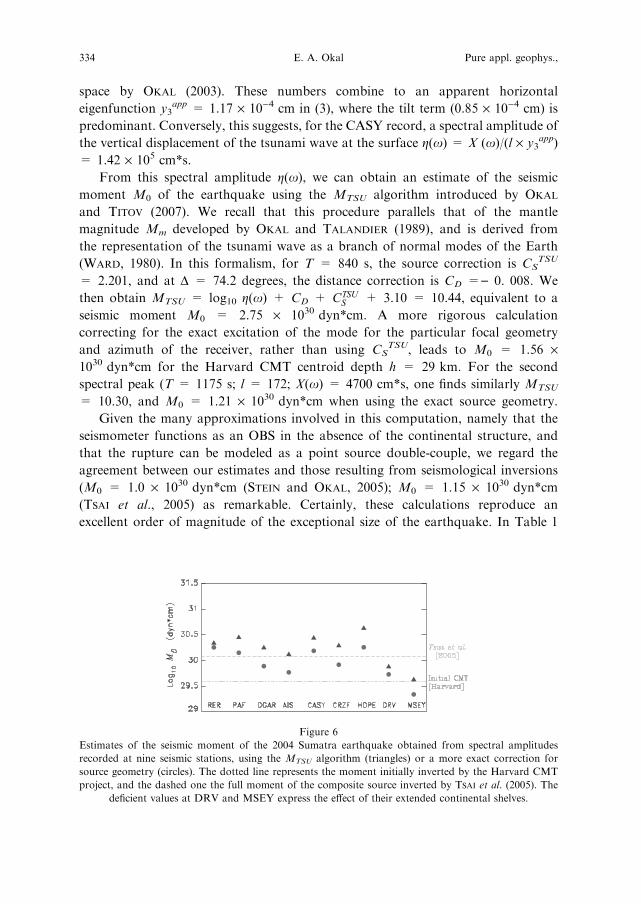
Figure 6

Estimates of the seismic moment of the 2004 Sumatra earthquake obtained from spectral amplitudes

recorded at nine seismic stations, using the MTSU algorithm (triangles) or a more exact correction for

source geometry (circles). The dotted line represents the moment initially inverted by the Harvard CMT

project, and the dashed one the full moment of the composite source inverted by TSAI et al. (2005). The

deficient values at DRV and MSEY express the effect of their extended continental shelves.

334 E. A. Okal Pure appl. geophys.,

and Figure 6, we extend our measurements to eight additional stations. At each

station, the moment is measured at the period featuring the spectral amplitude of

horizontal ground displacement with highest signal-to-noise ratio in the range 500–

5000 s; in practice these periods vary from 800 to 3000 seconds. We exclude

stations such as Bermuda and Scott Base for which the tsunami path around

continental masses departs significantly from a great circle. We also do not process

the record at Cocos Island, on which the timing of the arrivals is difficult to

reconcile with a definitive path, as already noted by YUAN et al. (2005). If we

further exclude the clearly deficient results at MSEY (Mahe, Seychelles) and DRV

(Dumont d’Urville, Antarctica), the geometrically averaged values of the moments

are 2.29 and 1.16 · 1030 dyn*cm, using the MTSU and full correction algorithms,

respectively, or only 0.30 ± 0.15 and 0.00 ± 0.18 logarithmic units over TSAI et

al.’s (2005) solution (dashed line on Fig. 6). In particular, all these measurements

suggest a moment several times larger than the original Harvard CMT solution of

3.95 · 1029 dyn*cm (dotted line on Fig. 6). They also confirm that the amplitude of

the tsunami in the far field is well accounted for by conventional mechanisms of

generation (once the exceptional size of the seismic moment is recognized), and

discount the need for ancillary mechanisms of excitation (influence of steep slopes

in the epicentral area; contribution of splay faults; large landslides).

We interpret the significant deficiencies of the solutions at MSEY, and to a

lesser extent at DRV, as site effects. Even though MSEY is within 2 km of the

shoreline, the Seychelles Islands have a continental structure (WEGENER, 1915; DU

TOIT, 1937; DAVIES, 1968), whose shelf extends about 120 km at sea in the

direction of arrival of the tsunami. Thus, the station cannot be regarded as coastal,

let alone as functioning as an OBS. Similarly, the extended continental shelf

seaward of DRV is probably responsible for the damping of the tsunami signal at

this otherwise coastal station.

We similarly attempted to invert a seismic moment from the spectral amplitudes

of the high-frequency components of the tsunami recorded at AIS, and described in

Section 2. We use the full source correction, since the the MTSU algorithm should

not be used at such periods, as the modeling of the correction CTSU was carried out

only in the 0.3–4 mHz frequency range (OKAL and TITOV, 2006). For amplitudes

X(x) � 500 and 1000 cm*s at the principal spectral peaks (T = 160 and 200 s), we

obtain M0 = 6.2 and 3.4 · 1029 dyn*cm, respectively. These values, especially the

second one, underestimate the moment of the event. We attribute this deficiency to

the significant depth extent of the source, for which the model of a point source,

legitimate at low frequencies (�1 mHz), becomes increasingly simplistic at

5–10 mHz, this effect being directly comparable to the deficiency affecting

conventional surface wave magnitudes MS when the source depth becomes

comparable to the wavelength.

Vol. 164, 2007 Seismic Records of the 2004 Sumatra Tsunamis 335

5. Application to Other Events

The purpose of this section is to apply the above formalisms to a selection of

other tsunamigenic earthquakes, in order to confirm the universal character of

seismic recordings of tsunamis, and to explore any possible quantitative correlation

between their amplitudes and the size of the parent earthquakes. All relevant

information is summarized in Table 3.

� The ‘‘Second’’ Sumatra (Nias) Earthquake of 28 March 2005

Although damaging in the near field, the tsunami generated by this earthquake

was deceptively small in the far field, a reflection of the shallow waters and large

islands present in the rupture area (SYNOLAKIS and ARCAS, quoted by KERR,

2005). Nevertheless, YUAN et al. (2005) did mention a seismic recording at

DGAR. We were able to detect the tsunami on seismic records at at least eight

stations, listed in Table 3, and to make spectral measurements at DGAR and

CRZF (at the other stations, the spectrum does not exhibit an appropriate signal-

to-noise ratio). While the seismic moment inverted from these records remains

large, it definitely characterizes the Nias earthquake as smaller than the 2004

Sumatra-Andaman one.

There are, however, significant differences between the seismic recordings of the

two Sumatra tsunamis. The 2005 tsunami was not recorded above noise level at the

Antarctic stations (CASY, DRV, SBA), and its record featured prominent ultra-long

period instabilities at MSEY. High-frequency components are not detected at

Amsterdam Island. Perhaps most astonishing is the timing of the signal at KIP,

around 15:20 on 29 March, or only 23 hours after origin time (Fig. 7), which would

correspond to eastward propagation, south of Australia, into the Tasman Sea and

the Southwest Pacific, rather than westward through the Drake Passage on 26

December, 2004. We have no explanation for this difference in routing between the

two tsunamis.

� The Peruvian Tsunami of 23 June 2001

This tsunami was damaging in the near field (OKAL et al., 2002), while its parent

earthquake was at the time the largest in the CMT catalogue (M0 = 4.7 · 1028 dyn-

cm), which it remained until the 2004 Sumatra earthquake. As shown on Figure 7a,

the tsunami is well recorded in the South central Pacific, from Pitcairn to Rarotonga.

Spectral measurements at RAR and PPT give an average moment only 11% larger

than the Harvard CMT solution.

The 2001 Peruvian tsunami was also recorded by the H2O observatory (CHAVE

et al., 2002) which operated on the ocean bottom about half way between Hawaii

and the Pacific Coast of the US from 1999 to 2003. The tsunami can be identified

in the spectrogram of the horizontal long-period component oriented N168�E

336 E. A. Okal Pure appl. geophys.,

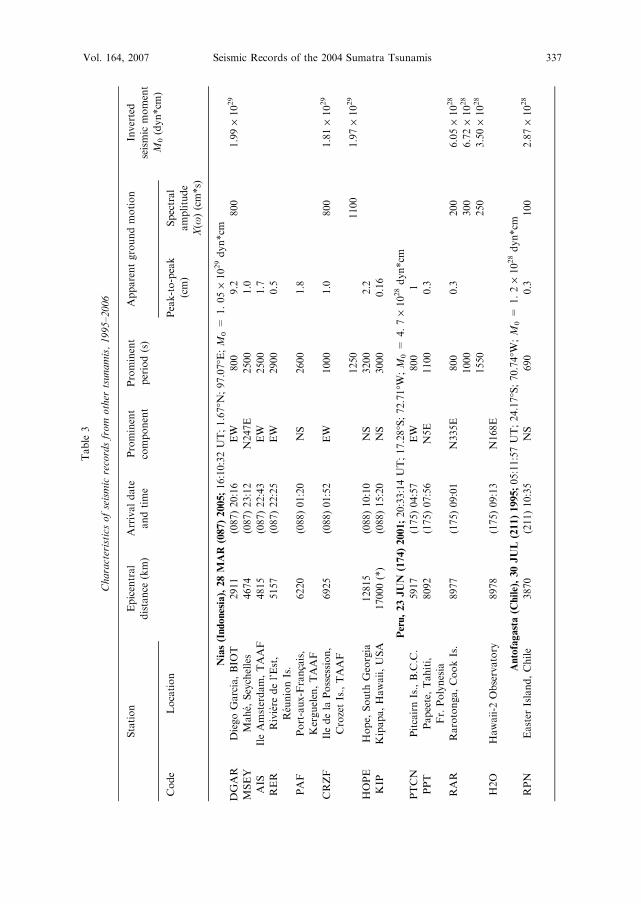
Table

3

Characteristics

ofseismic

recordsfrom

other

tsunamis,1995–2006

Station

Epicentral

distance

(km)

Arrivaldate

andtime

Prominent

component

Prominent

period(s)

Apparentgroundmotion

Inverted

seismic

moment

M0(dyn*cm

)

Code

Location

Peak-to-peak

(cm)

Spectral

amplitude

X(x

)(cm*s)

Nias(Indonesia),28MAR

(087)2005;16:10:32UT;1.67�N

;97.07�E

;M

0=

1.05

·1029dyn*cm

DGAR

DiegoGarcia,BIO

T2911

(087)20:16

EW

800

9.2

800

1.99

·1029

MSEY

Mahe,

Seychelles

4674

(087)23:12

N247E

2500

1.0

AIS

IleAmsterdam,TAAF

4815

(087)22:43

EW

2500

1.7

RER

Riviere

del’Est,

ReunionIs.

5157

(087)22:25

EW

2900

0.5

PAF

Port-aux-Francais,

Kerguelen,TAAF

6220

(088)01:20

NS

2600

1.8

CRZF

Iledela

Possession,

CrozetIs.,TAAF

6925

(088)01:52

EW

1000

1.0

800

1.81

·1029

1250

1100

1.97

·1029

HOPE

Hope,

South

Georgia

12815

(088)10:10

NS

3200

2.2

KIP

Kipapa,Hawaii,USA

17000(*)

(088)15:20

NS

3000

0.16

Peru,23JUN

(174)2001;20:33:14UT;17.28�S;72.71�W

;M

0=

4.7

·1028dyn*cm

PTCN

PitcairnIs.,B.C.C.

5917

(175)04:57

EW

800

1

PPT

Papeete,Tahiti,

Fr.Polynesia

8092

(175)07:56

N5E

1100

0.3

RAR

Rarotonga,CookIs.

8977

(175)09:01

N335E

800

0.3

200

6.05

·1028

1000

300

6.72

·1028

1550

250

3.50

·1028

H2O

Hawaii-2

Observatory

8978

(175)09:13

N168E

Antofagasta(C

hile),30JUL(211)1995;05:11:57UT;24.17�S;70.74�W

;M

0=

1.2

·1028dyn*cm

RPN

Easter

Island,Chile

3870

(211)10:35

NS

690

0.3

100

2.87

·1028

Vol. 164, 2007 Seismic Records of the 2004 Sumatra Tsunamis 337

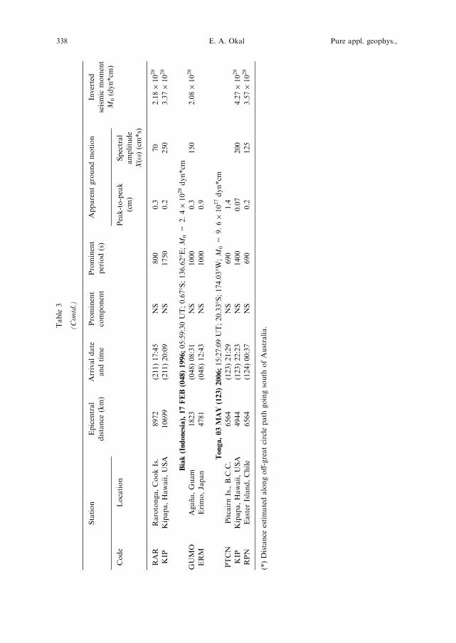
Table

3

(Contd.)

Station

Epicentral

distance

(km)

Arrivaldate

andtime

Prominent

component

Prominent

period(s)

Apparentgroundmotion

Inverted

seismic

moment

M0(dyn*cm

)

Code

Location

Peak-to-peak

(cm)

Spectral

amplitude

X(x

)(cm*s)

RAR

Rarotonga,CookIs.

8972

(211)17:45

NS

800

0.3

70

2.18

·1028

KIP

Kipapa,Hawaii,USA

10699

(211)20:09

NS

1750

0.2

250

3.37

·1028

Biak(Indonesia),17FEB(048)1996;05:59:30UT;0.67

�S;136.62�E

;M

0=

2.4

·1028dyn*cm

GUMO

Agana,Guam

1823

(048)08:31

NS

1000

0.3

150

2.08

·1028

ERM

Erimo,Japan

4781

(048)12:43

NS

1000

0.9

Tonga,03MAY

(123)2006;15:27:09UT;20.33�S;174.03�W

;M

0=

9.6

·1027dyn*cm

PTCN

PitcairnIs.,B.C.C.

6564

(123)21:29

NS

690

1.4

KIP

Kipapa,Hawaii,USA

4944

(123)22:23

NS

1400

0.07

200

4.27

·1028

RPN

Easter

Island,Chile

6564

(124)00:37

NS

690

0.2

125

3.57

·1028

(*)Distance

estimatedalongoff-greatcircle

path

goingsouth

ofAustralia.

338 E. A. Okal Pure appl. geophys.,

Kipapa, Hawaii, 28 March 2005 [Nias] Rarotonga, 30 July 1995 [Chile]

Rarotonga, 23 June 2001 [Peru] Agana, Guam, 17Feb.1996 [Biak] ˜

Hawaii-2 (H2O), 23 June 2001

a

b

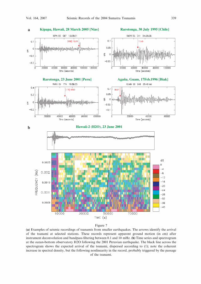
Figure 7

(a) Examples of seismic recordings of tsunamis from smaller earthquakes. The arrows identify the arrival

of the tsunami at selected stations. These records represent apparent ground motion (in cm) after

instrument deconvolution and bandpass filtering between 0.1 and 10 mHz. (b) Time series and spectrogram

at the ocean-bottom observatory H2O following the 2001 Peruvian earthquake. The black line across the

spectrogram shows the expected arrival of the tsunami, dispersed according to (1); note the coherent

increase in spectral density, but the following nonlinearity in the record, probably triggered by the passage

of the tsunami.

Vol. 164, 2007 Seismic Records of the 2004 Sumatra Tsunamis 339

(Fig. 7b), on the basis of the coherent rise in spectral density between 0.3 and

2 mHz at the group arrival times predicted by the dispersion relation (1). However,

the record suffers from obvious nonlinearity following this arrival and cannot be

processed quantitatively; it is possible that this instability was triggered by the

tsunami. Under the shallow water approximation, the ratio of velocity of

horizontal flow V in the water column to vertical surface displacement g is simply

V =g ¼ffiffiffiffiffiffiffiffiffi

g=Hp

, which predicts V on the order of a few mm/s. It is unclear whether

this would suffice to disturb the loose sedimentary structure in which the

instrument at H2O was deployed. Also, we note another occurrence of similar

instability much earlier in the time series.

� The Antofagasta, Chile Tsunami of 30 July 1995

This was the last Pacific tsunami with reported damage in the far field, as it

rocked a supply ship against the bottom of the harbor of Hakahau on Ua Pou in the

Marquesas Islands (GUIBOURG et al., 1997). The tsunami is well recorded on seismic

instruments from Easter Island to Western Samoa; however the record at AFI is

affected by strong nonlinearity. The average moment measured from spectral

amplitudes, M0 = 2.7 · 1028 dyn-cm, is about 2.3 times the CMT solution.

� The Biak, Indonesia Tsunami of 17 February 1996

This large earthquake (M0 = 2.4 · 1028 dyn*cm) generated a locally devastat-

ing tsunami which caused at least 120 deaths (MATSUTOMI et al., 2001), but was

recorded only marginally in the far field. We were able to identify a seismic

recording of the tsunami at Station GUMO (Agana, Guam), where the spectral

amplitude (150 cm*s at 1 mHz) leads to an excellent value of the seismic moment

(2.08 · 1028 dyn*cm). Unfortunately, Station KIP in Hawaii was down at that

time.

� The Tonga Tsunami of 03 May 2006

We also consider the case of this recent event, reminiscent of the 1977 intraslab

Tonga earthquake (TALANDIER and OKAL, 1979; LUNDGREN and OKAL, 1988),

300 km to the South. Despite a relatively deep focus (65 km), the tsunami is

detectable at seismic stations PTCN, RPN and KIP (at the time of writing, not all

South Pacific stations are available), and spectral amplitudes could be quantified at

the latter two.

These results are summarized on Figure 8, which compares seismic moments

inverted from spectral amplitudes of seismic recordings of the tsunamis to the

Harvard CMT solutions. This figure suggests a remarkable correlation, at least for

M0 ‡ 2 · 1028 dyn*cm, which serves to justify a posteriori the many assumptions used

in the present approach. It also confirms that the 2004 Sumatra earthquake was not

340 E. A. Okal Pure appl. geophys.,

anomalously tsunamigenic, and reconciles the amplitude of its tsunami with its

seismic source.

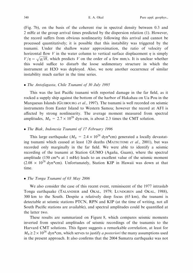
Finally, we examined the case of the Papua New Guinea tsunami of 17 July 1998.

The tsunami was catastrophic in the near field, with run-up reaching 15 m and

causing 2200 deaths, and is generally interpreted as resulting from an underwater

landslide triggered by the earthquake with a delay of 13 minutes (SYNOLAKIS et al.,

2002). Figure 9 shows that the tsunami is detectable on the EW component of the

regional station GUMO, between 1.5 and 3.5 mHz, with a dispersion of group times

suggesting propagation over an average water depth of 3 km, generally compatible

with the bathymetry of the shallow Eauripik Rise separating the East and West

Caroline Basins. However, the peak spectral amplitudes on this record (X(x) =

30 cm*s at T = 690 s and 2.5 cm*s at T = 330 s) lead to seismic moments of 6.1 ·1027 and 1.29 · 1028 dyn*cm, or 16 and 35 times the Harvard CMT solution,

Figure 8

Comparison of moments retrieved from spectral amplitudes of seismic records of six tsunamis with

published CMT solutions. For each earthquake, the gray circles are measurements at individual stations

(analogous to the circles on Fig. 6), and the squares the resulting geometrical average of the moments. In

the case of the 2004 Sumatra event, the deficient values at MSEY and DRV have been excluded.

Vol. 164, 2007 Seismic Records of the 2004 Sumatra Tsunamis 341

respectively. This confirms, if need be, that the 1998 Papua New Guinea tsunami

could not have been generated directly by the main shock. These observations

represent to our knowledge the first detection of the 1998 Papua New Guinea

Agana, Guam, 17 July 1998˜

Figure 9

Top: Time series of the EW long-period channel at Agana, Guam (GUMO) following the Papua New

Guinea earthquake of 17 July, 1998. The record is 25,000 s (� 7 hr) long. Center: Corresponding

spectrogram, showing arrival of tsunami �12,000 s into the time series with energy concentrated in the 1.2

to 3.5 mHz range. The black curve is the theoretical dispersion for propagation over a 3-km deep basin

from a source located at the Sissano amphitheater and and activated at 09:02 UTC (SYNOLAKIS et al.,

2002). Bottom: Equivalent surface wave amplitude g deconvolved from the top trace following the

procedure in Section 6, but bandpass filtered between 290 and 1000 s.

342 E. A. Okal Pure appl. geophys.,

tsunami at a distance (1809 km) falling outside the near field domain, which can be

used to support this conclusion.

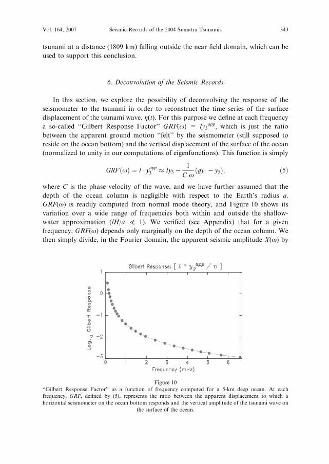
6. Deconvolution of the Seismic Records

In this section, we explore the possibility of deconvolving the response of the

seismometer to the tsunami in order to reconstruct the time series of the surface

displacement of the tsunami wave, g(t). For this purpose we define at each frequency

a so-called ‘‘Gilbert Response Factor’’ GRF(x) = ly3app, which is just the ratio

between the apparent ground motion ‘‘felt’’ by the seismometer (still supposed to

reside on the ocean bottom) and the vertical displacement of the surface of the ocean

(normalized to unity in our computations of eigenfunctions). This function is simply

GRF ðxÞ ¼ l � yapp3 � ly3 �

1

C xðgy1 � y5Þ; ð5Þ

where C is the phase velocity of the wave, and we have further assumed that the

depth of the ocean column is negligible with respect to the Earth’s radius a.

GRF(x) is readily computed from normal mode theory, and Figure 10 shows its

variation over a wide range of frequencies both within and outside the shallow-

water approximation (lH/a > 1). We verified (see Appendix) that for a given

frequency, GRF(x) depends only marginally on the depth of the ocean column. We

then simply divide, in the Fourier domain, the apparent seismic amplitude X(x) by

Figure 10

‘‘Gilbert Response Factor’’ as a function of frequency computed for a 5-km deep ocean. At each

frequency, GRF, defined by (5), represents the ratio between the apparent displacement to which a

horizontal seismometer on the ocean bottom responds and the vertical amplitude of the tsunami wave on

the surface of the ocean.

Vol. 164, 2007 Seismic Records of the 2004 Sumatra Tsunamis 343

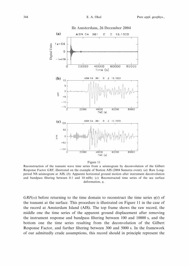
GRF(x) before returning to the time domain to reconstruct the time series g(t) ofthe tsunami at the surface. This procedure is illustrated on Figure 11 in the case of

the record at Amsterdam Island (AIS). The top frame shows the raw record, the

middle one the time series of the apparent ground displacement after removing

the instrument response and bandpass filtering between 100 and 10000 s, and the

bottom one the time series resulting from the deconvolution of the Gilbert

Response Factor, and further filtering between 300 and 5000 s. In the framework

of our admittedly crude assumptions, this record should in principle represent the

Ile Amsterdam, 26 December 2004(a)

(b)

(c)

Dig

ital U

nits

Figure 11

Reconstruction of the tsunami wave time series from a seismogram by deconvolution of the Gilbert

Response Factor GRF, illustrated on the example of Station AIS (2004 Sumatra event). (a): Raw Long-

period NS seismogram at AIS; (b): Apparent horizontal ground motion after instrument deconvolution

and bandpass filtering between 0.1 and 10 mHz; (c): Reconstructed time series of the sea surface

deformation, g.

344 E. A. Okal Pure appl. geophys.,

time series of the wave elevation g(t) of the surface of the ocean at the location, but

in the absence, of Amsterdam Island. Obviously, the high-frequency signal to the

left of the tsunami in the deconvolved trace should be ignored, as it represents the

result of processing the seismic surface waves from the earthquake through an

algorithm which is not applicable to them. This procedure was carried out for all

16 seismic records of the tsunami and the results, expressed as peak-to-peak g, arelisted in Table 1.

Unfortunately, no instruments capable of directly recording the 2004 Sumatra

tsunami on the high seas were operating at the time in the Indian Ocean, and thus it

is impossible to compare the results of our deconvolution to the actual height of the

tsunami. We nevertheless validate our algorithm in three different ways. First, we use

the record of the tsunami obtained by the JASON satellite altimeter which featured a

zero-to-peak amplitude of �70 cm (SCHARROO et al., 2005), on the same order of

magnitude as the deconvolved time series g on Figure 11 (85 cm). We emphasize,

however, the strong limitations of this comparison, given that the JASON trace is

neither a time nor a space series, and that it samples the tsunami several thousand km

to the north of AIS.

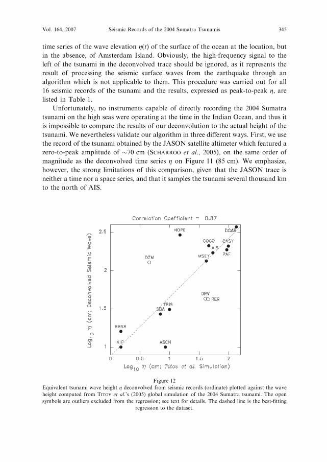
Figure 12

Equivalent tsunami wave height g deconvolved from seismic records (ordinate) plotted against the wave

height computed from TITOV et al.’s (2005) global simulation of the 2004 Sumatra tsunami. The open

symbols are outliers excluded from the regression; see text for details. The dashed line is the best-fitting

regression to the dataset.

Vol. 164, 2007 Seismic Records of the 2004 Sumatra Tsunamis 345

Second, we compare in Figure 12 the peak-to-peak amplitudes of our decon-

volved traces (listed in Table 1) to those computed as part of TITOV et al.’s (2005)

global simulation of the 2004 tsunami. Specifically, for each station, we extracted

from these authors’ database a time series at a ‘‘virtual gauge’’ located on the high

seas in the neighborhood of the station (typically 50 km out at sea, but with

allowances made for exceptional structures), and retained its peak-to-peak ampli-

tude, which we list as the last column of Table 1. The dataset is well correlated,

except for a number of intriguing outliers. Among them is Dumont d’Urville (DRV),

where we have already noted the deficient amplitude of the tsunami signal, possibly

due to the large continental shelf bordering the continent; the virtual gauge is located

seaward of the shelf. Both DZM in New Caledonia and RER in Reunion are the only

stations at substantial altitude (in both cases �800 m), which may affect their

response; we note however that one of them (DZM) has an enhanced response, the

other (RER) a deficient one. Excluding those three stations, we find a very strong

correlation (87%) between our deconvolved amplitudes and those simulated by

TITOV et al. (2005). However, we have no interpretation for the extreme amplitude

deconvolved at HOPE (although it may express some form of resonance of the

strongly indented Cumberland Bays where the station is located), nor for the extreme

deficiency at Ascension Island (ASCN). Also, we note that, while the deconvolved

amplitudes correlate with the simulated ones, the former remain generally several

times larger than the latter.

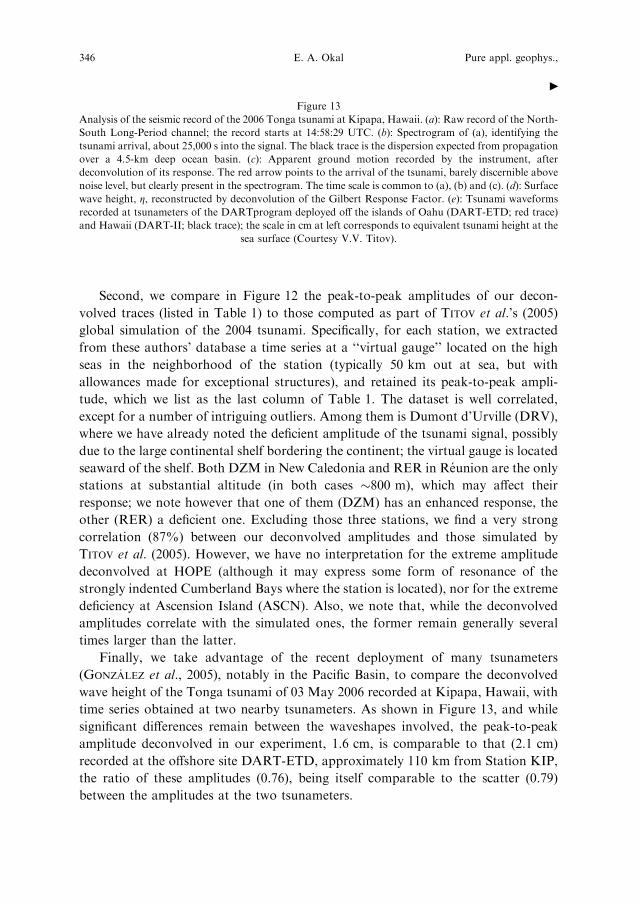
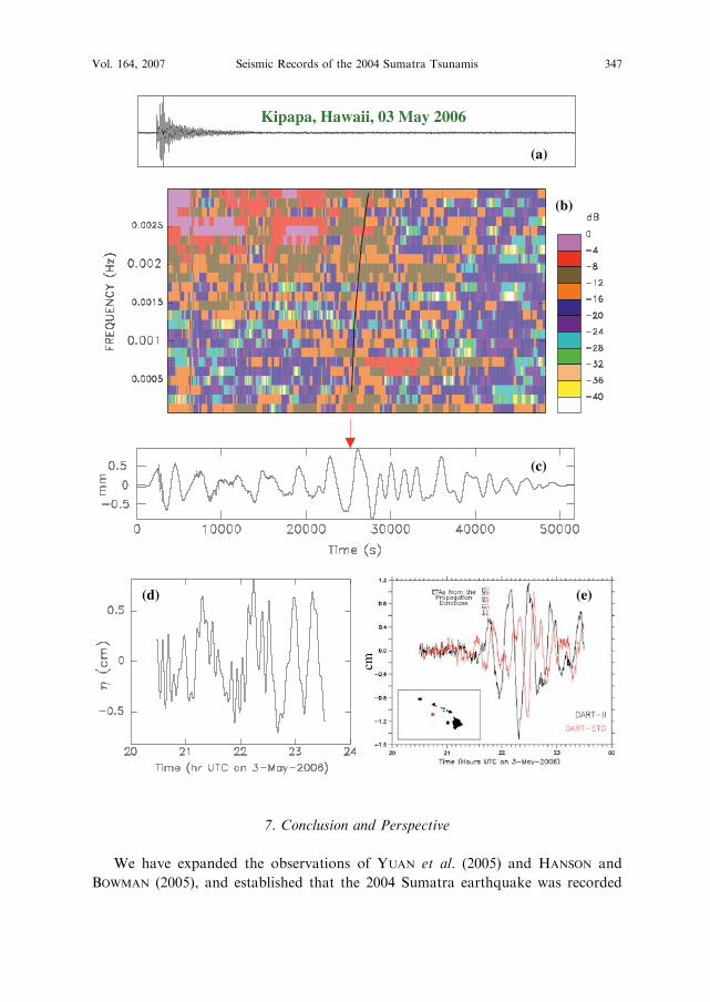
Finally, we take advantage of the recent deployment of many tsunameters

(GONZALEZ et al., 2005), notably in the Pacific Basin, to compare the deconvolved

wave height of the Tonga tsunami of 03 May 2006 recorded at Kipapa, Hawaii, with

time series obtained at two nearby tsunameters. As shown in Figure 13, and while

significant differences remain between the waveshapes involved, the peak-to-peak

amplitude deconvolved in our experiment, 1.6 cm, is comparable to that (2.1 cm)

recorded at the offshore site DART-ETD, approximately 110 km from Station KIP,

the ratio of these amplitudes (0.76), being itself comparable to the scatter (0.79)

between the amplitudes at the two tsunameters.

Figure 13

Analysis of the seismic record of the 2006 Tonga tsunami at Kipapa, Hawaii. (a): Raw record of the North-

South Long-Period channel; the record starts at 14:58:29 UTC. (b): Spectrogram of (a), identifying the

tsunami arrival, about 25,000 s into the signal. The black trace is the dispersion expected from propagation

over a 4.5-km deep ocean basin. (c): Apparent ground motion recorded by the instrument, after

deconvolution of its response. The red arrow points to the arrival of the tsunami, barely discernible above

noise level, but clearly present in the spectrogram. The time scale is common to (a), (b) and (c). (d): Surface

wave height, g, reconstructed by deconvolution of the Gilbert Response Factor. (e): Tsunami waveforms

recorded at tsunameters of the DARTprogram deployed off the islands of Oahu (DART-ETD; red trace)

and Hawaii (DART-II; black trace); the scale in cm at left corresponds to equivalent tsunami height at the

sea surface (Courtesy V.V. Titov).

c

346 E. A. Okal Pure appl. geophys.,

7. Conclusion and Perspective

We have expanded the observations of YUAN et al. (2005) and HANSON and

BOWMAN (2005), and established that the 2004 Sumatra earthquake was recorded

Kipapa, Hawaii, 03 May 2006

(a)

(b)

(c)

(e)(d)

cm

Vol. 164, 2007 Seismic Records of the 2004 Sumatra Tsunamis 347

essentially worldwide on the horizontal long-period channels of seismic stations

located in the vicinity (within �35 km) of shorelines. However, the recording can be

affected by site effects such as the presence of an extended continental shelf; large

bays can apparently enhance the signal (as at HOPE), or suppress it (as at ATD). At

intermediate ranges of distance (�4000 km), we show that seismometers can detect

the full spectrum of a tsunami branch, including their higher-frequency component

up to 10 mHz, which are strongly affected by dispersion outside the domain of

applicability of the shallow water approximation.

We have shown that it is possible to interpret seismic recordings of the

tsunami as representing the response of the seismometer to a deformation of the

ocean floor involving lateral displacement, tilt and gravitational potential, as

derived theoretically by GILBERT (1980). In this model, it is assumed that, for

stations located much closer to the shoreline than one wavelength, the progressive

wave is essentially unaltered from its structure on the high seas, with the result

that the instrument functions as an Ocean-Bottom Seismometer responding to the

tsunami in a deep basin. Estimates of the seismic moment of the parent

earthquake obtained in this framework and using standard normal mode theory

(WARD, 1980; OKAL, 1988, 2003) are in excellent agreement with published values,

which serves to justify the model, however outrageous the approximations

involved may sound.

In addition, we show that tsunami signals are present in the seismic

recordings of at least five more earthquakes, and that the seismic moments

derived from our algorithm scale remarkably well with published centroid-moment

tensor values.

The technique can be extended to a formal deconvolution of the seismic records

by removal of the Gilbert Response Function. On Figures 12 and 13, we found a

clear correlation between the amplitudes of the resulting time series and those

obtained from TITOV et al.’s [2005] global simulation (and in one case with a genuine

tsunameter record). This further confirms that such deconvolved signals are

representations of the tsunami wavefields on the high seas, and hence supports the

validity of the interpretation of the seismic recordings of the tsunamis. While this

requires a number of drastic simplifying assumptions, and notwithstanding the

potential importance of site effects at individual locations, the seismic instruments

have the great advantage of being for the most part already deployed on many

oceanic islands and continental shores, and in any case of coming at a fraction of the

deployment and above all maintenance costs of a network of bottom pressure

recorders linked to their open-seas buoys. The present study suggests that existing or

future broadband horizontal seismometers located near shore on oceanic islands or

continents could complement advantageously a network of buoy-based instruments

of the DART type.

348 E. A. Okal Pure appl. geophys.,

Acknowledgments

This research was supported by the National Science Foundation, under Grant

CMS-03-0154. I thank Rainer Kind for many discussions on this and other topics

in Potsdam in the Fall of 2005. I am grateful to Vasily Titov for access to the

database of global simulations of the Sumatra tsunami (TITOV et al., 2005), and for

the DART tsunameter records included in Figure 13. I thank Steve Ward for his

review of the original version of the paper, and in particular for his suggestion to

look at vertical records. Figure 1 was plotted using the GMT software (WESSEL

and SMITH, 1991).

Appendix

Tilt and Gravity Terms Compared for Seismic and Tsunami Modes

We compare here the various contributions from displacement, tilt and gravity to

the recording by long-period seismometers, of conventional seismic and tsunami

modes.

In addition to the response of a horizontal seismometer, given by equations (3) or

(4), we consider GILBERT’S (1980) expression for the response of a vertical

seismometer (his equation (4.12) p. 66):

AU ¼ x2 þ 2gr

� �

U þ lþ 1

rU; ðA-1Þ

which we rewrite in the formalism of SAITO (1967) as equivalent to the recording

of an apparent vertical displacement yapp1

yapp1 ¼ y1 þ

2grx2

y1 �lþ 1

rx2y5: ðA-2Þ

• For conventional seismic spheroidal modes, the second terms in (4) and (A-2) are

negligible as long as their period T remains less than 2pffiffiffiffiffiffiffiffiffiffi

a=2gp

� 1 hr, which is the

case of all mantle waves. As the latter carry very little gravitational energy, the

third terms are also negligible and for all practical purposes, y1app = y1; y3

app = y3;

the seismometer responds to ground motion. For the lowest frequency modes,

whose period approaches one hour, the contributions of the second and third

terms in (A-2) become important; however, because their signs are generally

opposite, the departure of y1app from y1 does not exceed 20% (for 0S2), as

Vol. 164, 2007 Seismic Records of the 2004 Sumatra Tsunamis 349

documented in GILBERT’S (1980) Table 1 (p. 66) or DAHLEN and TROMP’S (1998)

Table 10.1 (p. 375); the horizontal response would be affected more significantly

for the four gravest spheroidal modes, down to 0S5. Since few studies of the

fundamental spheroidal modes are conducted on horizontal instruments, and

toroidal modes are unaffected by such terms (GILBERT, 1980), the conclusion is

that tilt and gravity terms contribute marginally if at all to the recording of

conventional seismic modes. They do not affect the order of magnitude of the

recorded amplitude (this would happen only in the case of the yet-to-be observed

Slichter mode 1S1).

• We illustrate the case of tsunami modes by considering a typical period of 1014

seconds, corresponding to l ¼ 200 for an ocean depth of 4 km, overlying a solid

Earth inspired from PREM (DZIEWONSKI and ANDERSON, 1981). For a normal-

ization of the eigenfunction g = 1 cm at the surface of the ocean, we compute at

the ocean bottom y1 =) 0.0037 cm; y3 = 5.96 · 10)6 cm in the solid; and y5 =

0.0117 (cm/s)2. (Note that a negative value of y1 is expected, as it expresses the

downward vertical response of the elastic Earth to the overpressure accompanying

an upwards vertical displacement of the ocean surface.) In turn, these numbers

lead to a free air contribution (second term in (A-2)) of )2.98 · 10)4 cm (or only

8% of y1), and to a potential contribution (third term in (A-2)) of )9.66 · 10)3 cm

(or 2.6 times y1), the apparent displacement for a vertical seismometer being y1app

= ) 0.0137 cm. For the horizontal component, the tilt contribution to y3app

(second term in (4)) is 1.49 · 10)4 cm (25 times y3) and the potential contribution

(third term in (4)) is 4.81 · 10)5 cm (8 times y3), for a total y3 = 2.03 · 10)4 cm,

and an apparent displacement l y3app = 4.06 · 10)2 cm, i.e., three times the

amplitude of the vertical signal. This factor of three is further found to vary little

with frequency.

Seismic waves TSUNAMI

[363] 00:00

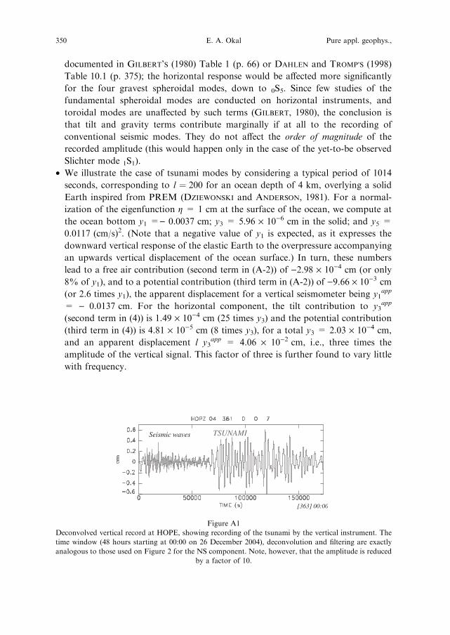
Figure A1

Deconvolved vertical record at HOPE, showing recording of the tsunami by the vertical instrument. The

time window (48 hours starting at 00:00 on 26 December 2004), deconvolution and filtering are exactly

analogous to those used on Figure 2 for the NS component. Note, however, that the amplitude is reduced

by a factor of 10.

350 E. A. Okal Pure appl. geophys.,

On Figure A1, we plot the vertical long-period seismogram at Hope, processed

in exactly the same fashion as the horizontal component on Figure 2. Note that the

tsunami is very prominent in this high-quality record, but that its amplitude is only

1/10 of its north-south counterpart, as opposed to the predicted 1/3. We cannot

explain this discrepancy by a factor of about three, but suspect that it may be

rooted in the different nature of the terms controlling the horizontal and vertical

responses. The former is completely governed by the tilt term, which depends only

on the wavelength of the tsunami mode, and as such may be more robust under the

extreme approximation made in assuming that the island seismometer behaves as

an OBS, while the vertical response is controlled principally by the potential term,

for which the approximation may not hold; note in particular that the missing

factor of three represents essentially the ratio y1app/y1 at the bottom of the ocean

(3.78). For this reason, we elect not to further study and attempt to quantify the

vertical records of the tsunami. However, we stress that they are indeed present.

Finally, we address the question of the sensitivity of the Gilbert Response

Function GRF to the height H of the ocean column. Under the Linear Shallow Water

Approximation, we have shown in OKAL (1982, 1988) that the eigenstress y2 at the

fluid-solid interface can be taken as y2 = )gqwg, and that in turn the vertical

displacement at the interface is y1 = y2/ Z with the impedance Z = 4/3 lk where l is

the rigidity of the substratum and k the wavenumber. As we discussed above, the

GRF is controlled by the tilt term in (4), leading to

GRF ¼ lyapp3

g� lg

rx2� 34

qwglk� 3

4� qwg2

l� 1x2

: ðA-3Þ

This expression is expected to be independent ofH, which we verified by recomputing

all the contributions to y1app and y3

app for an ocean depth H = 5 km, for which the

new value of l at 1014 s is 179, as opposed to (H = 4 km; l = 200) used above. We

find that y3app becomes 2.23 · 10)4 cm, and thus l y3

app = 3.99 · 10)2 cm, a decrease

of 1.7%, and for the vertical component, y1app =) 0.0139 cm, an absolute increase of

1.3% with respect to the case of the shallower ocean. Similar numbers are also found

across the frequency spectrum, and so we conclude that the effect of H on the Gilbert

Response Function GRF is negligible given the other approximations made in this

study.

REFERENCES

BEN-MENAHEM, A. and ROSENMAN, M. (1972), Amplitude patterns of tsunami waves from submarine

earthquakes, J. Geophys. Res. 77, 3097–3128.

CHAVE, A.D., DUENNEBIER, F.K., BUTLER, R., PETITT, R.A., Jr., WOODING, F.B., HARRIS, D., BAILEY,

J.W., HOBART, E., JOLLY, J., BOWEN, A.D. and YOERGER, D.R., H2O: The Hawaii-2 Observatory. In

Vol. 164, 2007 Seismic Records of the 2004 Sumatra Tsunamis 351

Science-technology Synergy for Research in the Marine Environment: Challenges for the XXIst Century

(eds. L. Beranzoli, P. Favali, and G. Smriglio), Devel. Mar. Tech. Ser., 12, pp. 83–92 (Elsevier,

Amsterdam, 2002).

DAHLEN, F.A. and TROMP, J. Theoretical Seismology (Princeton Univ. Press, 1998, 1025 pp.)

DAVIES, D. (1968), When did the Seychelles leave India? Nature 220, 1225–1226.

DU TOIT, A.L., Our Wandering Continents, 366 pp. (Oliver & Boyd, London, 1937).

DZIEWONSKI, A.M. and ANDERSON, D.L. (1981), Preliminary Earth Reference Model, Phys. Earth Planet.

Inter. 25, 297–356.

GILBERT, F., An introduction to low-frequency seismology. In Proc. Intl. School Phys. ‘‘Enrico Fermi’’, 78

(eds. A.M. Dziewonski and E. Boschi), pp. 41–81 (North Holland, Amsterdam, 1980).

GONZALEZ, F.I., BERNARD, E.N., MEINIG, C., EBLE, M.C., MOFJELD, H.O. and STALIN, S. (2005), The

NTHMP Tsunameter network, Natural Hazards 35, 25–39.

GUIBOURG, S., HEINRICH, P., and ROCHE, R. (1997), Numerical modeling of the 1995 Chilean tsunami.

Impact on French Polynesia, Geophys. Res. Lett. 24, 775–778.

HANSON J.A. and BOWMAN, J.R. (2005), Dispersive and reflected tsunami signals from the 2004 Indian

Ocean tsunami observed on hydrophones and seismic stations, Geophys. Res. Lett. 32(17), L17606, 5 pp.

KERR, R.A. (2005),Model shows islands muted tsunami after latest Indonesian earthquake, Science 308, 341.

LA ROCCA, M., GALLUZZO, D., SACCOROTTI, G., TINTI, S., CIMINI, G.B., and DEL PEZZO E. (2004),

Seismic signals associated with landslides and with a tsunami at Stromboli Volcano, Italy, Bull. Seismol.

Soc. Amer. 94, 1850–1867.

LUNDGREN, P.R. and OKAL, E.A. (1988), Slab decoupling in the Tonga arc: the June 22, 1977 earthquake,

J. Geophys. Res. 93, 13355–13366.

MATSUTOMI, H., SHUTO, N., IMAMURA, F., and TAKAHASHI, T. (2001), Filed survey of the 1996 Irian Jaya

earthquake tsunami on Biak Island, Nat. Haz. 24, 199–212.

OKAL, E.A. (1982), Mode-wave equivalence and other asymptotic problems in tsunami theory, Phys. Earth

Planet. Inter. 30, 1–11.

Okal, E.A. (1988), Seismic parameters controlling far-field tsunami amplitudes: A review, Natural Hazards

1, 67–96.

OKAL, E.A. (1991), Erratum [to ‘‘Seismic parameters controlling far-field tsunami amplitudes: A review’’],

Natural Hazards 4, 433.

OKAL, E.A. (2003), Normal modes energetics for far-field tsunamis generated by dislocations and landslides,

Pure Appl. Geophys. 160, 2189–2221.

OKAL, E.A. and TALANDIER, J. (1989),Mm: A variable period mantle magnitude, J. Geophys. Res. 94, 4169–

4193.

OKAL, E.A. and TITOV, V.V. (2007), MTSU: Recovering seismic moments from tsunameter records, Pure

Appl. Geophys., 164, 355–378.

OKAL, E.A., DENGLER, L., ARAYA, S., BORRERO, J.C., GOMER, B., KOSHIMURA, S., LAOS, G., OLCESE, D.,

ORTIZ, M., SWENSSON, M., TITOV, V.V., and Vegas, F. (2002), A field survey of the Camana, Peru tsunami

of June 23, 2001, Seismol. Res. Lett. 73, 904–917.

OKAL, E.A., FRITZ, H.M., RAVELOSON, R., JOELSON, G., PANCOSKOVA, P., and RAMBOLAMANANA, G.

(2006a), Field survey of the 2004 Indonesian tsunami in Madagascar, Earthquake Spectra 22, S263–S283.

OKAL, E.A., SLADEN, A., and OKAL, E.A.-S. (2006b), Field survey of the 2004 Indonesian tsunami on

Rodrigues, Mauritius, and Reunion Islands, Earthquake Spectra 22, S241–S261.

OKAL, E.A., TALANDIER, J., and REYMOND, D. (2007) Quantification of hydrophone records of the 2004

Sumatra tsunami, Pure Appl. Geophys. 164, 309–323.

SAITO, M. (1967), Excitation of free oscillations and surface waves by a point source in a vertically

heterogeneous Earth, J. Geophys. Res. 72, 3689–3699.

SATAKE, K. (1988), Effects of bathymetry on tsunami propagation: Application of ray tracing to tsunamis,

Pure Appl. Geophys. 126, 28–35.

SCHARROO, R., SMITH, W.H.F., TITOV, V.V., and ARCAS, D. (2005) Observing the Indian Ocean tsunami

with satellite altimetry, Geophys. Res. Abstr. 7, 230 (abstract).

STEIN, S. and OKAL, E.A. (2005), Size and speed of the Sumatra earthquake, Nature 434, 581–582.

352 E. A. Okal Pure appl. geophys.,

SYNOLAKIS, C.E., BARDET, J.-P., BORRERO, J.C., DAVIES, H.L., OKAL, E.A., SILVER, E.A., SWEET, S., and

TAPPIN, D.R. (2002), The slump origin of the 1998 Papua New Guinea tsunami, Proc. Roy. Soc. (London),

Ser. A 458, 763–789.

TALANDIER, J. and OKAL, E.A. (1979), Human perception of T waves: the June 22, 1977 Tonga earthquake

felt on Tahiti, Bull. Seismol. Soc. Amer. 69,1475–1486.

TITOV, V.V., RABINOVICH, A.B., MOFJELD, H.O., THOMSON, R.E., and GONZALEZ, F.I. (2005), The global

reach of the 26 December 2004 Sumatra tsunami, Science 309, 2045–2048.

TSAI, V.C., NETTLES, M., EKSTROM, G., and DZIEWONSKI, A.M. (2005), Multiple CMT source analysis of

the 2004 Sumatra earthquake, Geophys. Res. Lett. 32(17), L17304, 4 pp.

WARD, S.N. (1980), Relationships of tsunami generation and an earthquake source, J. Phys. Earth 28, 441–

474.

WEGENER, A.L., Die Entstehung der Kontinente und Ozeane (Vieweg, Braunschweig, 1915).

WOODS, M.T. and OKAL, E.A. (1987) Effect of variable bathymetry on the amplitude of teleseismic tsunamis:

a ray-tracing experiment, Geophys. Res. Lett. 14, 765–768.

WESSEL, P. and SMITH, W.H.F. (1991), Free software helps map and display data, Eos, Trans. Amer. Geo-

phys. Un. 72, 441 and 445–446.

YUAN, X., KIND, R., and PEDERSEN, H. (2005), Seismic monitoring of the Indian Ocean tsunami, Geophys.

Res. Lett. 32(15), L15308, 4 pp.

(Received May 29, 2006, accepted July 30, 2006)

To access this journal online:

http://www.birkhauser.ch

Vol. 164, 2007 Seismic Records of the 2004 Sumatra Tsunamis 353