seismic modeling, migration and velocity · pdf fileseismic modeling, migration and velocity...
TRANSCRIPT
Seismic Modeling, Migration and VelocityInversion
The Partial Differential Wave Equations
Bee Bednar
Panorama Technologies, Inc.14811 St Marys Lane, Suite 150
Houston TX 77079
May 30, 2014
Bee Bednar (Panorama Technologies) Seismic Modeling, Migration and Velocity Inversion May 30, 2014 1 / 29

Outline
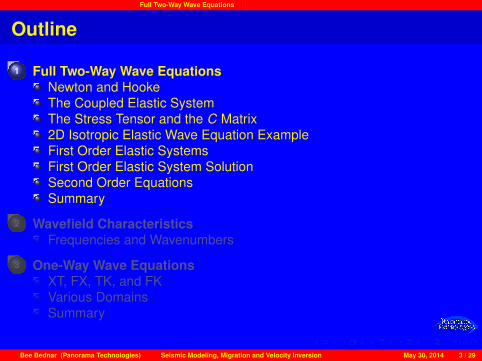
1 Full Two-Way Wave EquationsNewton and HookeThe Coupled Elastic SystemThe Stress Tensor and the C Matrix2D Isotropic Elastic Wave Equation ExampleFirst Order Elastic SystemsFirst Order Elastic System SolutionSecond Order EquationsSummary
2 Wavefield CharacteristicsFrequencies and Wavenumbers
3 One-Way Wave EquationsXT, FX, TK, and FKVarious DomainsSummary
Bee Bednar (Panorama Technologies) Seismic Modeling, Migration and Velocity Inversion May 30, 2014 2 / 29
Full Two-Way Wave Equations
Outline
1 Full Two-Way Wave EquationsNewton and HookeThe Coupled Elastic SystemThe Stress Tensor and the C Matrix2D Isotropic Elastic Wave Equation ExampleFirst Order Elastic SystemsFirst Order Elastic System SolutionSecond Order EquationsSummary
2 Wavefield CharacteristicsFrequencies and Wavenumbers
3 One-Way Wave EquationsXT, FX, TK, and FKVarious DomainsSummary
Bee Bednar (Panorama Technologies) Seismic Modeling, Migration and Velocity Inversion May 30, 2014 3 / 29

Full Two-Way Wave Equations Newton and Hooke
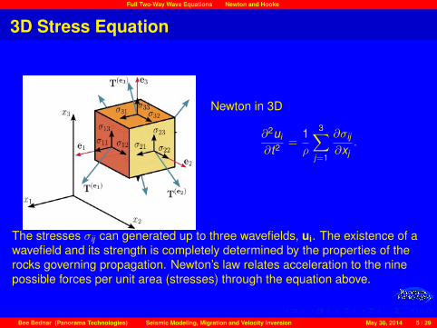
3D Stress Equation
Newton in 3D
∂2ui
∂t2 =1ρ
3∑j=1
∂σij
∂xj.
In 3D,the forces that can affect a point are in-line compressional andorthogonal shear. Looking at a small cube each of the nine faces of the cubecan move both inward and outward as compressional as well as shear alongvertical and horizontal planes.
Bee Bednar (Panorama Technologies) Seismic Modeling, Migration and Velocity Inversion May 30, 2014 4 / 29
Full Two-Way Wave Equations Newton and Hooke
3D Stress Equation
Newton in 3D
∂2ui
∂t2 =1ρ
3∑j=1
∂σij
∂xj.
The stresses σij can generated up to three wavefields, ui. The existence of awavefield and its strength is completely determined by the properties of therocks governing propagation. Newton’s law relates acceleration to the ninepossible forces per unit area (stresses) through the equation above.
Bee Bednar (Panorama Technologies) Seismic Modeling, Migration and Velocity Inversion May 30, 2014 5 / 29

Full Two-Way Wave Equations Newton and Hooke
3D Hooke
For a linear 3D medium, Hooke’s law can be rephrased asA CHANGE in FORCE per unit volume is equal to the bulk modulustimes the increase in volume divided by the original volume.
The 3D stress equation has nine stress factors, σij , one for each of the threedimensions and three coupled wavefields, ui . Hooke’s law says that
each component of stress σij is linearly proportional to everycomponent of strain Emn
so that
σij =∑m,n
cijmnEmn =∑m,n
cijmn12
(∂um
∂xn+∂un
∂xm
)In this case the cijmn are elements of what is called the stress tensor.
Bee Bednar (Panorama Technologies) Seismic Modeling, Migration and Velocity Inversion May 30, 2014 6 / 29

Full Two-Way Wave Equations The Coupled Elastic System
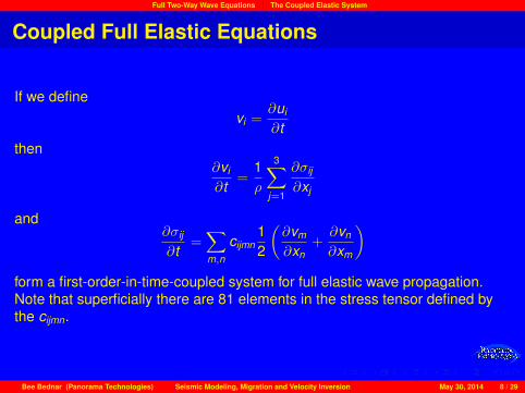
Coupled Full Elastic Equations
The two equations∂2ui
∂t2 =1ρ
3∑j=1
∂σij
∂xj
σij =∑m,n
cijmn12
(∂um
∂xn+∂un
∂xm
)form a coupled system for full elastic wave propagation. Note that superficiallythere are 81 elements in the stress tensor defined by the cijmn.
Bee Bednar (Panorama Technologies) Seismic Modeling, Migration and Velocity Inversion May 30, 2014 7 / 29
Full Two-Way Wave Equations The Coupled Elastic System
Coupled Full Elastic Equations
If we definevi =
∂ui
∂tthen
∂vi
∂t=
1ρ
3∑j=1
∂σij
∂xj
and∂σij
∂t=∑m,n
cijmn12
(∂vm
∂xn+∂vn
∂xm
)form a first-order-in-time-coupled system for full elastic wave propagation.Note that superficially there are 81 elements in the stress tensor defined bythe cijmn.
Bee Bednar (Panorama Technologies) Seismic Modeling, Migration and Velocity Inversion May 30, 2014 8 / 29
Full Two-Way Wave Equations The Stress Tensor and the C Matrix
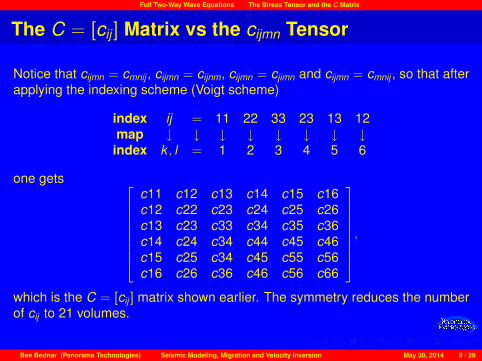
The C = [cij ] Matrix vs the cijmn Tensor
Notice that cijmn = cmnij , cijmn = cijnm, cijmn = cjimn and cijmn = cmnij , so that afterapplying the indexing scheme (Voigt scheme)
index ij = 11 22 33 23 13 12map ↓ ↓ ↓ ↓ ↓ ↓ ↓ ↓index k , l = 1 2 3 4 5 6
one gets c11 c12 c13 c14 c15 c16c12 c22 c23 c24 c25 c26c13 c23 c33 c34 c35 c36c14 c24 c34 c44 c45 c46c15 c25 c34 c45 c55 c56c16 c26 c36 c46 c56 c66
,
which is the C = [cij ] matrix shown earlier. The symmetry reduces the numberof cij to 21 volumes.
Bee Bednar (Panorama Technologies) Seismic Modeling, Migration and Velocity Inversion May 30, 2014 9 / 29

Full Two-Way Wave Equations 2D Isotropic Elastic Wave Equation Example
2D Isotropic Elastic Wave Equation
As an example, the 2D Isotropic Elastic Wave Equation is
∂v1∂t = 1
ρ
(∂σ1,1∂x1
+∂σ1,3∂x3
)∂v3∂t = 1
ρ
(∂σ1,3∂x1
+∂σ3,3∂x3
)∂σ1,1∂t = λ+2µ
ρ∂v1∂x1
+ λρ∂v3∂x3
∂σ1,3∂t = µ
ρ
(∂v3∂x1
+ ∂v1∂x3
)∂σ3,3∂t = λ+2µ
ρ∂v3∂x3
+ λρ∂v1∂x1
where, in the usual geophysical notation, x1 = x , and x3 = z. Thus, v1represents particle velocity in the horizontal and v3 is particle velocity in thevertical direction. In this case the C matrix is defined by λ+ 2µ and µ. Notethat these are actually 2D numeric fields. That is, they are 2D functions of xand z.
Bee Bednar (Panorama Technologies) Seismic Modeling, Migration and Velocity Inversion May 30, 2014 10 / 29
Full Two-Way Wave Equations First Order Elastic Systems
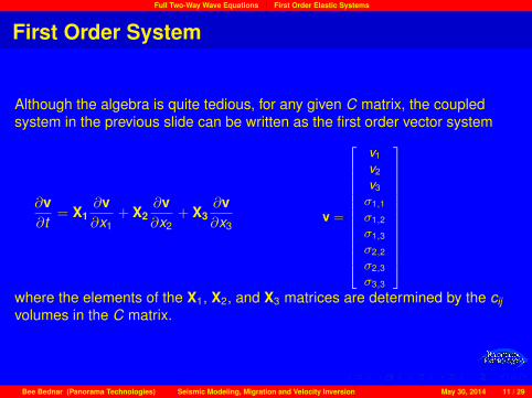
First Order System
Although the algebra is quite tedious, for any given C matrix, the coupledsystem in the previous slide can be written as the first order vector system
∂v∂t
= X1∂v∂x1
+ X2∂v∂x2
+ X3∂v∂x3
v =
26666666666664
v1
v2
v3
σ1,1
σ1,2
σ1,3
σ2,2
σ2,3
σ3,3
37777777777775where the elements of the X1, X2, and X3 matrices are determined by the cijvolumes in the C matrix.
Bee Bednar (Panorama Technologies) Seismic Modeling, Migration and Velocity Inversion May 30, 2014 11 / 29
Full Two-Way Wave Equations First Order Elastic System Solution
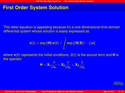
First Order System Solution
This latter equation is appealing because it’s a one-dimensional-time-domaindifferential system whose solution is easily expressed as
v(t) = exp [tH] v(0) +
t∫0
exp [ξH] S(t − ξ)dξ
where v(0) represents the initial conditions, S(t) is the source term and H isthe operator
H = X1∂
∂x1+ X2
∂
∂x2+ X3
∂
∂x3
Bee Bednar (Panorama Technologies) Seismic Modeling, Migration and Velocity Inversion May 30, 2014 12 / 29
Full Two-Way Wave Equations Second Order Equations
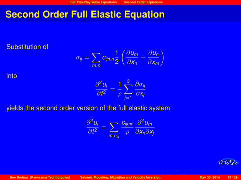
Second Order Full Elastic Equation
Substitution of
σij =∑m,n
cijmn12
(∂um
∂xn+∂un
∂xm
)into
∂2ui
∂t2 =1ρ
3∑j=1
∂σij
∂xj
yields the second order version of the full elastic system
∂2ui
∂t2 =∑m,n,j
cijmn
ρ
∂2um
∂xn∂xj
Bee Bednar (Panorama Technologies) Seismic Modeling, Migration and Velocity Inversion May 30, 2014 13 / 29

Full Two-Way Wave Equations Second Order Equations
Second Order Isotropic Elastic Equation
When the C matrix represents a isotropic elastic system, the two shear ortransverse waves are identical, so, after considerable algebraic manipulation,one can write
∂2u∂t2 = (
λ+ 2µρ
)∇(∇ · u)− µ
ρ∇×∇× u
where the first component of u = (u1,u3) is the compressional wave and thethird component is the transverse or shear wave. From a physical viewpoint,the dot product annihilates the compressional component, while the crossproduct annihilates the shear component.
Bee Bednar (Panorama Technologies) Seismic Modeling, Migration and Velocity Inversion May 30, 2014 14 / 29
Full Two-Way Wave Equations Second Order Equations
Second Order Scalar Wave Equation
In a purely acoustic media, the shear parameters are zero, so there is nopropagation of shear waves. The 3D elastic equation reduces to the scalarform
∂2u∂t2 =
λ
ρ
(∂2u∂x2 +
∂2u∂y2 +
∂2u∂z2
)Setting v =
√λρ produces the traditional scalar wave equation.
Bee Bednar (Panorama Technologies) Seismic Modeling, Migration and Velocity Inversion May 30, 2014 15 / 29

Full Two-Way Wave Equations Summary
Two-Way Wave Equation Summary
In the interest of clarity, the previous derivations were performed under someoverly simplistic assumptions. Most notably was the assumption that thedensity, ρ, was constant as a function of position. Had this not been the case,the full scalar wave equation would have taken the form
∂2p∂t2 = ρv2
[∂
∂x1ρ
∂p∂x
+∂
∂y1ρ
∂p∂y
+∂
∂z1ρ
∂p∂z
].
and the fully elastic wave equation would have been a bit more complex.Fortunately, this assumption will not significantly impair out ability tounderstand the computational aspects of digital wave propagation, so thediscussion is continued with the equations as previously derived. Theanisotropic models of interest are VTI, TTI, ORT , and TORT , all of which areincorporated within the fully elastic wave equation.
Bee Bednar (Panorama Technologies) Seismic Modeling, Migration and Velocity Inversion May 30, 2014 16 / 29

Full Two-Way Wave Equations Summary
Two-Way Wave Equation Summary
There are two fundamental wave equation styles:
Scalar∂2p∂t2 = ρv2
[∂
∂x1ρ
∂p∂x
+∂
∂y1ρ
∂p∂y
+∂
∂z1ρ
∂p∂z
]and vector
∂σij
∂t=
∑m,n
cijmn12
(∂vm
∂xn+∂vn
∂xm
)∂vi
∂t=
1ρ
3∑j=1
∂σij
∂xj
Bee Bednar (Panorama Technologies) Seismic Modeling, Migration and Velocity Inversion May 30, 2014 17 / 29
Full Two-Way Wave Equations Summary
Two-Way Wave Equation Summary
Its worth noting that every seismic wave equation of interest can be derivedfrom the coupled system
∂σij
∂t=
∑m,n
cijmn12
(∂vm
∂xn+∂vn
∂xm
)∂vi
∂t=
1ρ
3∑j=1
∂σij
∂xj
so technically this is the only system of concern.
Bee Bednar (Panorama Technologies) Seismic Modeling, Migration and Velocity Inversion May 30, 2014 18 / 29

Wavefield Characteristics
Outline
1 Full Two-Way Wave EquationsNewton and HookeThe Coupled Elastic SystemThe Stress Tensor and the C Matrix2D Isotropic Elastic Wave Equation ExampleFirst Order Elastic SystemsFirst Order Elastic System SolutionSecond Order EquationsSummary
2 Wavefield CharacteristicsFrequencies and Wavenumbers
3 One-Way Wave EquationsXT, FX, TK, and FKVarious DomainsSummary
Bee Bednar (Panorama Technologies) Seismic Modeling, Migration and Velocity Inversion May 30, 2014 19 / 29
Wavefield Characteristics Frequencies and Wavenumbers
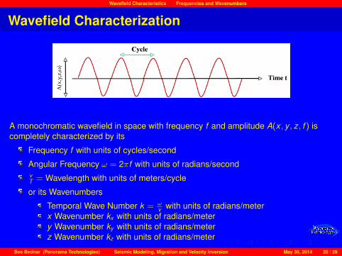
Wavefield Characterization
A monochromatic wavefield in space with frequency f and amplitude A(x , y , z, f ) iscompletely characterized by its
Frequency f with units of cycles/second
Angular Frequency ω = 2πf with units of radians/secondvf = Wavelength with units of meters/cycle
or its Wavenumbers
Temporal Wave Number k = ωv with units of radians/meter
x Wavenumber kx with units of radians/metery Wavenumber ky with units of radians/meterz Wavenumber kz with units of radians/meter
Bee Bednar (Panorama Technologies) Seismic Modeling, Migration and Velocity Inversion May 30, 2014 20 / 29
Wavefield Characteristics Frequencies and Wavenumbers
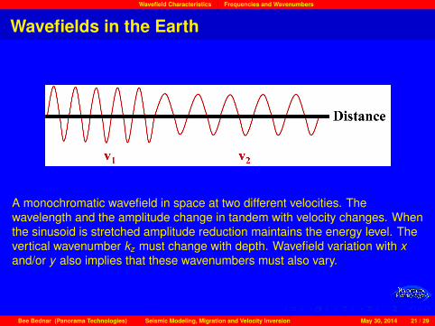
Wavefields in the Earth
A monochromatic wavefield in space at two different velocities. Thewavelength and the amplitude change in tandem with velocity changes. Whenthe sinusoid is stretched amplitude reduction maintains the energy level. Thevertical wavenumber kz must change with depth. Wavefield variation with xand/or y also implies that these wavenumbers must also vary.
Bee Bednar (Panorama Technologies) Seismic Modeling, Migration and Velocity Inversion May 30, 2014 21 / 29
Wavefield Characteristics Frequencies and Wavenumbers
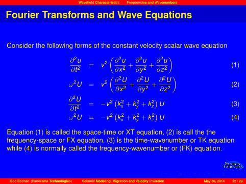
Fourier Transforms and Wave Equations
Consider the following forms of the constant velocity scalar wave equation
∂2u∂t2 = v2
(∂2u∂x2 +
∂2u∂y2 +
∂2u∂z2
)(1)
ω2U = v2(∂2U∂x2 +
∂2U∂y2 +
∂2U∂z2
)(2)
∂2U∂t2 = −v2 (k2
x + k2y + k2
z)
U (3)
ω2U = −v2 (k2x + k2
y + k2z)
U (4)
Equation (1) is called the space-time or XT equation, (2) is call the thefrequency-space or FX equation, (3) is the time-wavenumber or TK equationwhile (4) is normally called the frequency-wavenumber or (FK) equation.
Bee Bednar (Panorama Technologies) Seismic Modeling, Migration and Velocity Inversion May 30, 2014 22 / 29

One-Way Wave Equations
Outline
1 Full Two-Way Wave EquationsNewton and HookeThe Coupled Elastic SystemThe Stress Tensor and the C Matrix2D Isotropic Elastic Wave Equation ExampleFirst Order Elastic SystemsFirst Order Elastic System SolutionSecond Order EquationsSummary
2 Wavefield CharacteristicsFrequencies and Wavenumbers
3 One-Way Wave EquationsXT, FX, TK, and FKVarious DomainsSummary
Bee Bednar (Panorama Technologies) Seismic Modeling, Migration and Velocity Inversion May 30, 2014 23 / 29

One-Way Wave Equations XT, FX, TK, and FK
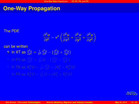
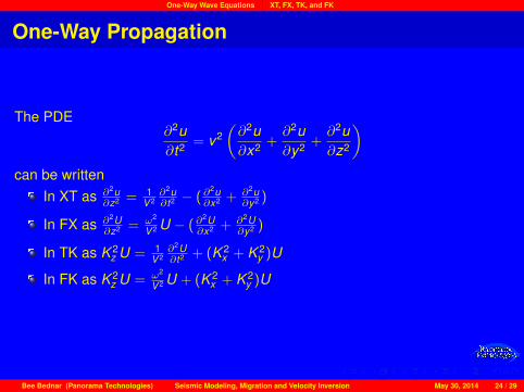
One-Way Propagation
The PDE∂2u∂t2 = v2
(∂2u∂x2 +
∂2u∂y2 +
∂2u∂z2
)can be written
In XT as ∂2u∂z2 = 1
V 2∂2u∂t2 − (∂
2u∂x2 + ∂2u
∂y2 )
In FX as ∂2U∂z2 = ω2
V 2 U − (∂2U∂x2 + ∂2U
∂y2 )
In TK as K 2z U = 1
V 2∂2U∂t2 + (K 2
x + K 2y )U
In FK as K 2z U = ω2
V 2 U + (K 2x + K 2
y )U
Bee Bednar (Panorama Technologies) Seismic Modeling, Migration and Velocity Inversion May 30, 2014 24 / 29
One-Way Wave Equations XT, FX, TK, and FK
One-Way Propagation
The PDE∂2u∂t2 = v2
(∂2u∂x2 +
∂2u∂y2 +
∂2u∂z2
)can be written
In XT as ∂2u∂z2 = 1
V 2∂2u∂t2 − (∂
2u∂x2 + ∂2u
∂y2 )
In FX as ∂2U∂z2 = ω2
V 2 U − (∂2U∂x2 + ∂2U
∂y2 )
In TK as K 2z U = 1
V 2∂2U∂t2 + (K 2
x + K 2y )U
In FK as K 2z U = ω2
V 2 U + (K 2x + K 2
y )U
Bee Bednar (Panorama Technologies) Seismic Modeling, Migration and Velocity Inversion May 30, 2014 24 / 29
One-Way Wave Equations Various Domains
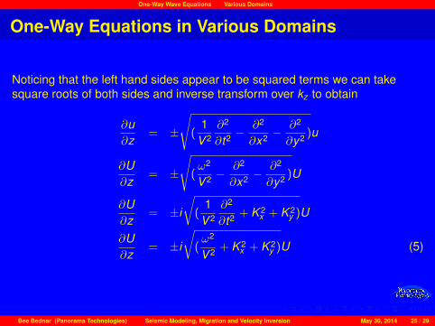
One-Way Equations in Various Domains
Noticing that the left hand sides appear to be squared terms we can takesquare roots of both sides and inverse transform over kz to obtain
∂u∂z
= ±
√(
1V 2
∂2
∂t2 −∂2
∂x2 −∂2
∂y2 )u
∂U∂z
= ±
√(ω2
V 2 −∂2
∂x2 −∂2
∂y2 )U
∂U∂z
= ±i
√(
1V 2
∂2
∂t2 + K 2x + K 2
y )U
∂U∂z
= ±i
√(ω2
V 2 + K 2x + K 2
y )U (5)
Bee Bednar (Panorama Technologies) Seismic Modeling, Migration and Velocity Inversion May 30, 2014 25 / 29
One-Way Wave Equations Various Domains
One-Way Propagation
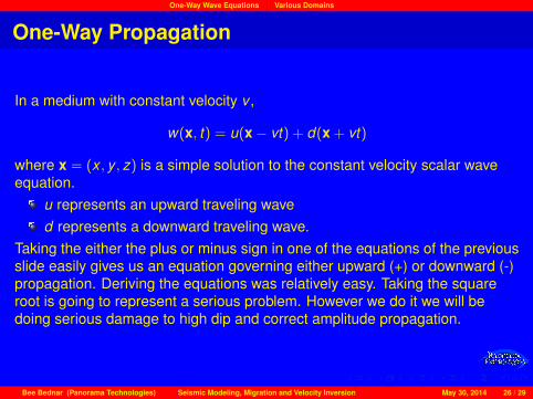
In a medium with constant velocity v ,
w(x, t) = u(x− vt) + d(x + vt)
where x = (x , y , z) is a simple solution to the constant velocity scalar waveequation.
u represents an upward traveling waved represents a downward traveling wave.
Taking the either the plus or minus sign in one of the equations of the previousslide easily gives us an equation governing either upward (+) or downward (-)propagation. Deriving the equations was relatively easy. Taking the squareroot is going to represent a serious problem. However we do it we will bedoing serious damage to high dip and correct amplitude propagation.
Bee Bednar (Panorama Technologies) Seismic Modeling, Migration and Velocity Inversion May 30, 2014 26 / 29
One-Way Wave Equations Summary
One-Way Equation Summary
Used for both isotropic and anisotropic propagationFor full elastic one-way propagation
Based on an equation with vs = 0Very non-physicalStanding wave noiseLower quality amplitudes and dips
Bee Bednar (Panorama Technologies) Seismic Modeling, Migration and Velocity Inversion May 30, 2014 27 / 29
One-Way Wave Equations Summary
One-Way Propagation
Why?Increases efficiencyStep down one ∆z at a time
Why not?Dips limited to 90 degreesNo multiplesNo RefractionsAmplitude distortion
Bee Bednar (Panorama Technologies) Seismic Modeling, Migration and Velocity Inversion May 30, 2014 28 / 29

One-Way Wave Equations Summary
Questions?
Bee Bednar (Panorama Technologies) Seismic Modeling, Migration and Velocity Inversion May 30, 2014 29 / 29