4.2 Seismic methods

33

4.2 Seismic methods

Seismic measurements are well known from their use in hydrocarbon exploration, but can also be applied for mapping of shallower underground structures such as buried valleys. The method is comparable to a marine echo sounder: seismic waves are created by a hit on the surface and they travel underground. Like sound waves, they are reflected and refracted when they reach a boundary between different layers in the underground. Using the time required for the wave to come back to the surface and the velocity of travel, we can determine the depth of different geological boundaries. The velocity value of the waves carries information on the type of sediment or rock. This method is important not only for structural information, e.g. in delineating faults or valley structures, but also for physical characterization of layers and thus is very useful in hydrogeological investigations. Since the 1920’s, seismic reflection techniques have been used to search for petroleum and refraction techniques have been used in engineering applications. Additionally, since the 1980’s, significant strides have been made in both near-surface seismic reflection surveying and in the development of shallow-seismic refraction methods. Near-surface methods use an adaptation of parameters to high resolution information – that is the capacity to discriminate layers – and may provide results also from layers that are 500 m in depth, such as deep buried valleys. The main references for this Section are Pelton (2005), Steeples (2005), various chapters on seismic methods in Knödel et al. (1997), Rabbel (2006), Yilmaz (2001). 4.2.1 Physical base

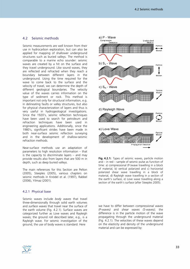
Seismic waves include body waves that travel three-dimensionally through solid earth volumes and surface waves that travel near the surface of the earth volume (Fig. 4.2.1). Surface waves are categorized further as Love waves and Rayleigh waves; the ground roll described later, e.g., is a Rayleigh wave. For seismic investigation of the ground, the use of body waves is standard. Here

Fig. 4.2.1: Types of seismic waves, particle motion and – in red – sample of seismic pulse as function of time: a) compressional (P-)wave travelling in a block of material, b) vertical polarized and c) horizontal polarized shear wave travelling in a block of material, d) Rayleigh wave travelling in a section of the earth‘s surface, e) Love wave travelling along a section of the earth’s surface (after Steeples 2005).

we have to differ between compressional waves (P-waves) and shear waves (S-waves); the difference is in the particle motion of the wave propagating through the underground material (Fig. 4.2.1). The velocities of these waves depend on the elasticity and density of the underground material and can be expressed by:

HELGA WIEDERHOLD

34

ρμ3

4+k=VP (4.2.1)

ρμ=VS (4.2.2)

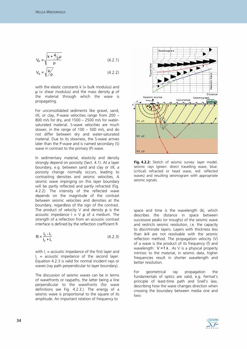
with the elastic constants k (= bulk modulus) and μ (= shear modulus) and the mass density ρ of the material through which the wave is propagating. For unconsolidated sediments like gravel, sand, till, or clay, P-wave velocities range from 200 – 800 m/s for dry, and 1500 – 2500 m/s for water-saturated material. S-wave velocities are much slower, in the range of 100 – 500 m/s, and do not differ between dry and water-saturated material. Due to its slowness, the S-wave arrives later than the P-wave and is named secondary (S) wave in contrast to the primary (P) wave. In sedimentary material, elasticity and density strongly depend on porosity (Sect. 4.1). At a layer boundary, e.g. between sand and clay or till, a porosity change normally occurs, leading to contrasting densities and seismic velocities. A seismic wave impinging on this layer boundary will be partly reflected and partly refracted (Fig. 4.2.2). The intensity of the reflected wave depends on the magnitude of the contrast between seismic velocities and densities at the boundary, regardless of the sign of the contrast. The product of velocity V and density ρ is the acoustic impedance I = V ρ of a medium. The strength of a reflection from an acoustic contrast interface is defined by the reflection coefficient R

12

12

I+III

=R-

(4.2.3)

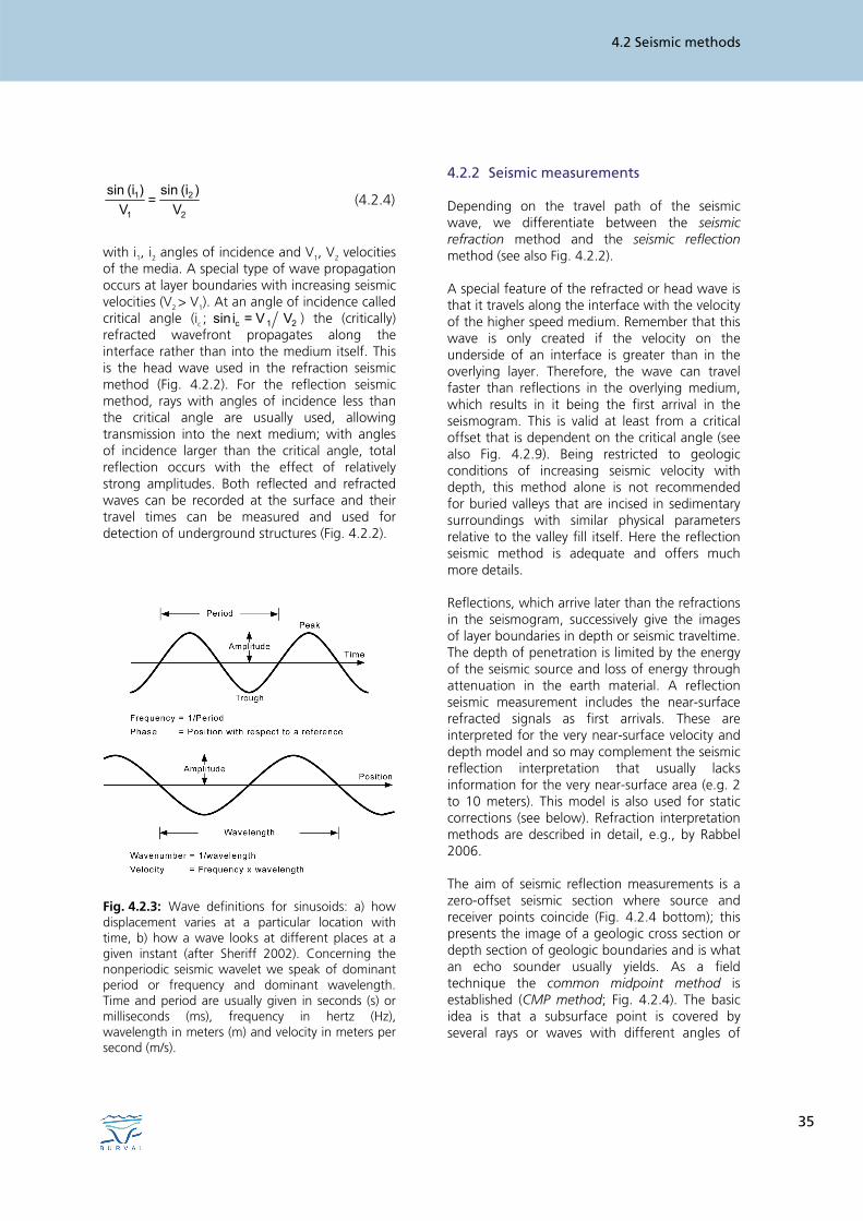
with I1 = acoustic impedance of the first layer and I2 = acoustic impedance of the second layer. Equation 4.2.3 is valid for normal incident rays or waves (ray path perpendicular to layer boundary). The discussion of seismic waves can be in terms of wavefronts or raypaths, the latter being a line perpendicular to the wavefronts (for wave definitions see Fig. 4.2.3.). The energy of a seismic wave is proportional to the square of its amplitude. An important relation of frequency to

Fig. 4.2.2: Sketch of seismic survey: layer model, seismic rays (green: direct travelling wave, blue: (critical) refracted or head wave, red: reflected waves) and resulting seismogram with appropriate seismic signals.

space and time is the wavelength (λ), which describes the distance in space between successive peaks (or troughs) of the seismic wave and restricts seismic resolution, i.e. the capacity to discriminate layers. Layers with thickness less than λ/4 are not resolvable with the seismic reflection method. The propagation velocity (V) of a wave is the product of its frequency (f) and wavelength: λf=V . As V is a physical property intrinsic to the material, in seismic data, higher frequencies result in shorter wavelength and better resolution. For geometrical ray propagation the fundamentals of optics are valid, e.g. Fermat’s principle of least-time path and Snell’s law, describing how the wave changes direction when crossing the boundary between media one and two:

4.2 Seismic methods

35

2

2

1

1

V)i(sin

=V

)i(sin (4.2.4)

with i1, i2 angles of incidence and V1, V2 velocities of the media. A special type of wave propagation occurs at layer boundaries with increasing seismic velocities (V2 > V1). At an angle of incidence called critical angle (ic ; 21c VV=isin ) the (critically) refracted wavefront propagates along the interface rather than into the medium itself. This is the head wave used in the refraction seismic method (Fig. 4.2.2). For the reflection seismic method, rays with angles of incidence less than the critical angle are usually used, allowing transmission into the next medium; with angles of incidence larger than the critical angle, total reflection occurs with the effect of relatively strong amplitudes. Both reflected and refracted waves can be recorded at the surface and their travel times can be measured and used for detection of underground structures (Fig. 4.2.2).

Fig. 4.2.3: Wave definitions for sinusoids: a) how displacement varies at a particular location with time, b) how a wave looks at different places at a given instant (after Sheriff 2002). Concerning the nonperiodic seismic wavelet we speak of dominant period or frequency and dominant wavelength. Time and period are usually given in seconds (s) or milliseconds (ms), frequency in hertz (Hz), wavelength in meters (m) and velocity in meters per second (m/s).

4.2.2 Seismic measurements

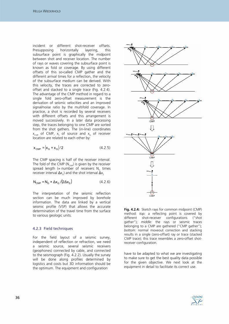
Depending on the travel path of the seismic wave, we differentiate between the seismic refraction method and the seismic reflection method (see also Fig. 4.2.2). A special feature of the refracted or head wave is that it travels along the interface with the velocity of the higher speed medium. Remember that this wave is only created if the velocity on the underside of an interface is greater than in the overlying layer. Therefore, the wave can travel faster than reflections in the overlying medium, which results in it being the first arrival in the seismogram. This is valid at least from a critical offset that is dependent on the critical angle (see also Fig. 4.2.9). Being restricted to geologic conditions of increasing seismic velocity with depth, this method alone is not recommended for buried valleys that are incised in sedimentary surroundings with similar physical parameters relative to the valley fill itself. Here the reflection seismic method is adequate and offers much more details. Reflections, which arrive later than the refractions in the seismogram, successively give the images of layer boundaries in depth or seismic traveltime. The depth of penetration is limited by the energy of the seismic source and loss of energy through attenuation in the earth material. A reflection seismic measurement includes the near-surface refracted signals as first arrivals. These are interpreted for the very near-surface velocity and depth model and so may complement the seismic reflection interpretation that usually lacks information for the very near-surface area (e.g. 2 to 10 meters). This model is also used for static corrections (see below). Refraction interpretation methods are described in detail, e.g., by Rabbel 2006. The aim of seismic reflection measurements is a zero-offset seismic section where source and receiver points coincide (Fig. 4.2.4 bottom); this presents the image of a geologic cross section or depth section of geologic boundaries and is what an echo sounder usually yields. As a field technique the common midpoint method is established (CMP method; Fig. 4.2.4). The basic idea is that a subsurface point is covered by several rays or waves with different angles of

HELGA WIEDERHOLD

36

incident or different shot-receiver offsets. Presupposing horizontally layering, this subsurface point is graphically the midpoint between shot and receiver location. The number of rays or waves covering the subsurface point is known as fold or coverage. By using different offsets of this so-called CMP gather and the different arrival times for a reflection, the velocity of the subsurface medium can be derived. With this velocity, the traces are corrected to zero-offset and stacked to a single trace (Fig. 4.2.4). The advantage of the CMP method in regard to a single fold zero-offset measurement is the derivation of seismic velocities and an improved signal/noise ratio by the multifold coverage. In practice, a shot is recorded by several receivers with different offsets and this arrangement is moved successively. In a later data processing step, the traces belonging to one CMP are sorted from the shot gathers. The (in-line) coordinates xCMP of CMP, xS of source and xG of receiver location are related to each other by:

2/x+x=x GSCMP (4.2.5)

The CMP spacing is half of the receiver interval. The fold of the CMP (NCMP) is given by the receiver spread length (= number of receivers NG times receiver interval ΔxG) and the shot interval ΔxS

( )SGGCMP xΔ2/xΔ×N=N (4.2.6)

The interpretation of the seismic reflection section can be much improved by borehole information. The data are linked by a vertical seismic profile (VSP) that allows the accurate determination of the travel time from the surface to various geologic units. 4.2.3 Field techniques

For the field layout of a seismic survey, independent of reflection or refraction, we need a seismic source, several seismic receivers (geophones) connected by cable, and connected to the seismograph (Fig. 4.2.2). Usually the survey will be done along profiles determined by logistics and costs but 3D information should be the optimum. The equipment and configuration

Fig. 4.2.4: Sketch rays for common midpoint (CMP) method: top: a reflecting point is covered by different shot-receiver configurations (“shot gather”); middle: the rays or seismic traces belonging to a CMP are gathered (“CMP gather”); bottom: normal moveout correction and stacking results in a single (zero-offset) ray or trace (stacked CMP trace); this trace resembles a zero-offset shot-receiver configuration.

have to be adapted to what we are investigating to make sure to get the best quality data possible for the given objective. We next look at the equipment in detail to facilitate its correct use.

4.2 Seismic methods

37

Seismic source

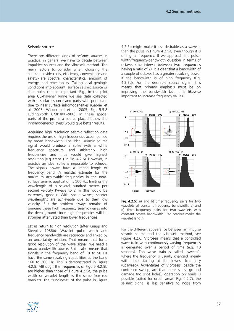
There are different kinds of seismic sources in practice; in general we have to decide between impulsive sources and the vibroseis method. The main factors to consider when choosing the source - beside costs, efficiency, convenience and safety - are spectral characteristics, amount of energy, and repeatability. Taking local geologic conditions into account, surface seismic source or shot holes can be important. E.g., in the pilot area Cuxhavener Rinne we see data collected with a surface source and parts with poor data due to near surface inhomogeneities (Gabriel et al. 2003, Wiederhold et al. 2005; Fig. 5.5.8 Lüdingworth CMP 800–900). In these special parts of the profile a source placed below the inhomogeneous layers would give better results. Acquiring high resolution seismic reflection data requires the use of high frequencies accompanied by broad bandwidth. The ideal seismic source signal would produce a spike with a white frequency spectrum and arbitrarily high frequencies and thus would give highest resolution (e.g. trace 1 in Fig. 4.2.6). However, in practice an ideal spike is impossible to achieve. The signals always have a limited length or frequency band. A realistic estimate for the maximum achievable frequencies in the near-surface seismic application is 500 Hz, limiting the wavelength of a several hundred meters per second velocity P-wave to 2 m (this would be extremely good!). With shear waves, shorter wavelengths are achievable due to their low velocity. But the problem always remains of bringing these high frequency seismic waves into the deep ground since high frequencies will be stronger attenuated than lower frequencies. Let us return to high resolution (after Knapp and Steeples 1986b): Wavelet pulse width and frequency bandwidth are reciprocal and linked by an uncertainty relation. That means that for a good resolution of the wave signal, we need a broad bandwidth source. But it also means that signals in the frequency band of 10 to 50 Hz have the same resolving capabilities as the band 160 to 200 Hz. This is demonstrated in Figure 4.2.5. Although the frequencies of Figure 4.2.5b are higher than those of Figure 4.2.5a, the pulse width or wavelet length is the same (see red bracket). The “ringiness” of the pulse in Figure

4.2.5b might make it less desirable as a wavelet than the pulse in Figure 4.2.5a, even though it is of higher frequency. If we approach the pulse-width/frequency-bandwidth question in terms of octaves (the interval between two frequencies having a ratio of 2), it is clear that a bandwidth of a couple of octaves has a greater resolving power if the bandwidth is of high frequency (Fig. 4.2.5d). For the desirable source signal, this means that primary emphasis must be on improving the bandwidth but it is likewise important to increase frequency values.

Fig. 4.2.5: a) and b) time-frequency pairs for two wavelets of constant frequency bandwidth; c) and d) time frequency pairs for two wavelets with constant octave bandwidth. Red bracket marks the wavelet length.

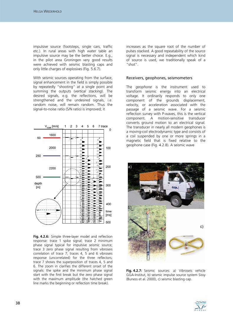
For the different appearance between an impulse seismic source and the vibroseis method, see Figure 4.2.6. Vibroseis means that a controlled wave train with continuously varying frequencies is generated over a period of time (e.g. 10 seconds). This wave train is called “sweep”, where the frequency is usually changed linearly with time starting at the lowest frequency (upsweep). Advantages of Vibroseis, beside the controlled sweep, are that there is less ground damage (no shot holes), operation on roads is possible (suited for urban areas; Fig. 4.2.7), the seismic signal is less sensitive to noise from

HELGA WIEDERHOLD

38

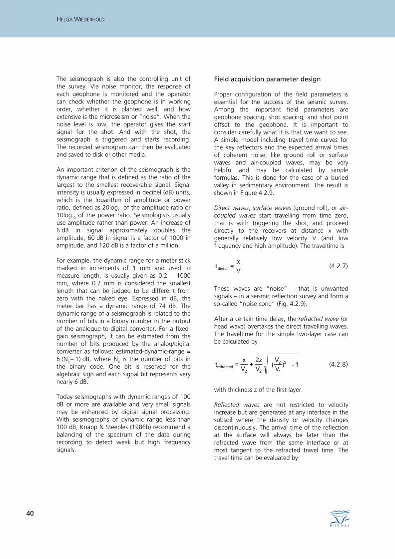
impulsive source (footsteps, single cars, traffic etc.). In rural areas with high water table an impulsive source may be the better choice. E.g., in the pilot area Groningen very good results were achieved with seismic blasting caps and only little charges of explosives (Fig. 5.6.7). With seismic sources operating from the surface, signal enhancement in the field is simply possible by repeatedly “shooting” at a single point and summing the outputs (vertical stacking). The desired signals, e.g. the reflections, will be strengthened and the undesired signals, i.e. random noise, will remain random. Thus the signal-to-noise ratio (S/N ratio) is improved; it

Fig. 4.2.6: Simple three-layer model and reflection response: trace 1 spike signal; trace 2 minimum phase signal typical for impulsive seismic source; trace 3 zero phase signal resulting from vibroseis correlation of trace 7; traces 4, 5 and 6 vibroseis response (uncorrelated) for the three reflectors; trace 7 shows the superposition of traces 4, 5 and 6. The zoom in clarifies the different onset of the signals: the spike and the minimum phase signal start with the first break but the zero phase signal with the maximum amplitude (the hatched green line marks the beginning or reflection time break).

increases as the square root of the number of pulses stacked. A good repeatability of the source signal is necessary and independent which kind of source is used, we traditionally speak of a “shot”. Receivers, geophones, seismometers

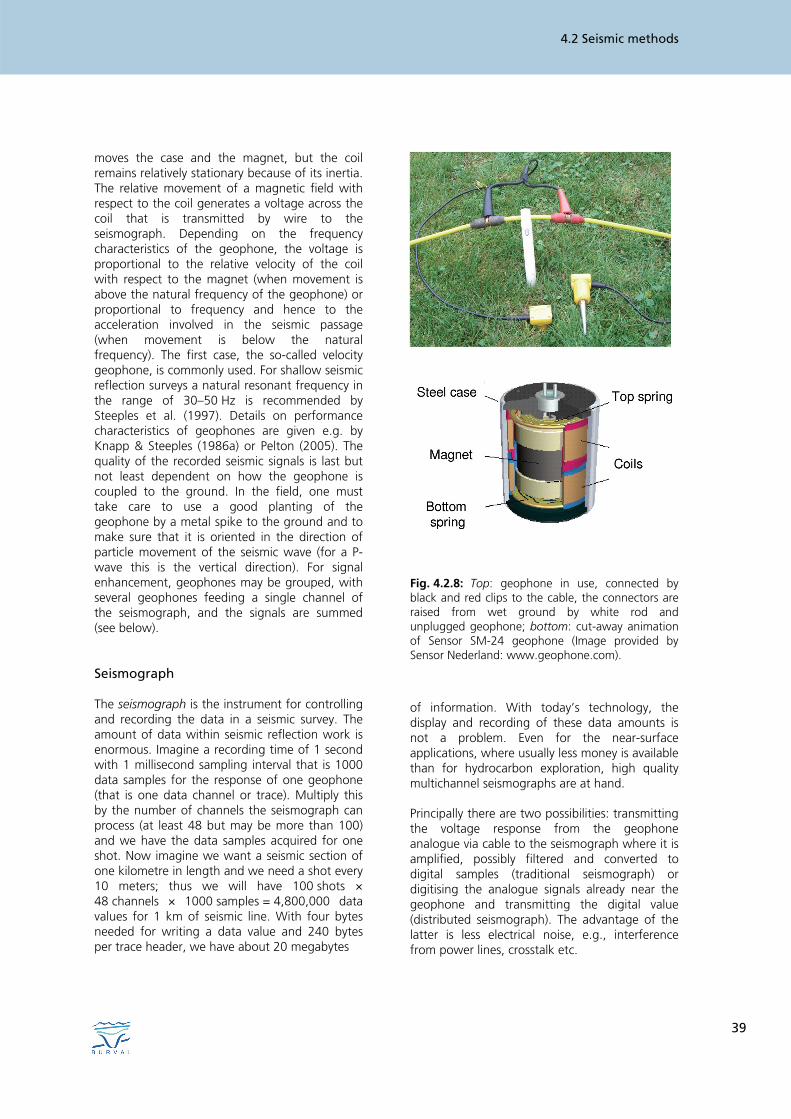
The geophone is the instrument used to transform seismic energy into an electrical voltage. It ordinarily responds to only one component of the grounds displacement, velocity, or acceleration associated with the passage of a seismic wave. For a seismic reflection survey with P-waves, this is the vertical component. A motion-sensitive transducer converts ground motion to an electrical signal. The transducer in nearly all modern geophones is a moving-coil electrodynamic type and consists of a coil suspended by one or more springs in a magnetic field that is fixed relative to the geophone case (Fig. 4.2.8). A seismic wave

Fig. 4.2.7: Seismic sources: a) Vibroseis vehicle GGA-Institut, b) seismic impulse source system Sissy (Buness et al. 2000), c) seismic blasting cap.

4.2 Seismic methods

39

moves the case and the magnet, but the coil remains relatively stationary because of its inertia. The relative movement of a magnetic field with respect to the coil generates a voltage across the coil that is transmitted by wire to the seismograph. Depending on the frequency characteristics of the geophone, the voltage is proportional to the relative velocity of the coil with respect to the magnet (when movement is above the natural frequency of the geophone) or proportional to frequency and hence to the acceleration involved in the seismic passage (when movement is below the natural frequency). The first case, the so-called velocity geophone, is commonly used. For shallow seismic reflection surveys a natural resonant frequency in the range of 30–50 Hz is recommended by Steeples et al. (1997). Details on performance characteristics of geophones are given e.g. by Knapp & Steeples (1986a) or Pelton (2005). The quality of the recorded seismic signals is last but not least dependent on how the geophone is coupled to the ground. In the field, one must take care to use a good planting of the geophone by a metal spike to the ground and to make sure that it is oriented in the direction of particle movement of the seismic wave (for a P-wave this is the vertical direction). For signal enhancement, geophones may be grouped, with several geophones feeding a single channel of the seismograph, and the signals are summed (see below). Seismograph

The seismograph is the instrument for controlling and recording the data in a seismic survey. The amount of data within seismic reflection work is enormous. Imagine a recording time of 1 second with 1 millisecond sampling interval that is 1000 data samples for the response of one geophone (that is one data channel or trace). Multiply this by the number of channels the seismograph can process (at least 48 but may be more than 100) and we have the data samples acquired for one shot. Now imagine we want a seismic section of one kilometre in length and we need a shot every 10 meters; thus we will have 100 shots × 48 channels × 1000 samples = 4,800,000 data values for 1 km of seismic line. With four bytes needed for writing a data value and 240 bytes per trace header, we have about 20 megabytes

Fig. 4.2.8: Top: geophone in use, connected by black and red clips to the cable, the connectors are raised from wet ground by white rod and unplugged geophone; bottom: cut-away animation of Sensor SM-24 geophone (Image provided by Sensor Nederland: www.geophone.com).

of information. With today’s technology, the display and recording of these data amounts is not a problem. Even for the near-surface applications, where usually less money is available than for hydrocarbon exploration, high quality multichannel seismographs are at hand. Principally there are two possibilities: transmitting the voltage response from the geophone analogue via cable to the seismograph where it is amplified, possibly filtered and converted to digital samples (traditional seismograph) or digitising the analogue signals already near the geophone and transmitting the digital value (distributed seismograph). The advantage of the latter is less electrical noise, e.g., interference from power lines, crosstalk etc.

HELGA WIEDERHOLD

40

The seismograph is also the controlling unit of the survey. Via noise monitor, the response of each geophone is monitored and the operator can check whether the geophone is in working order, whether it is planted well, and how extensive is the microseism or “noise”. When the noise level is low, the operator gives the start signal for the shot. And with the shot, the seismograph is triggered and starts recording. The recorded seismogram can then be evaluated and saved to disk or other media. An important criterion of the seismograph is the dynamic range that is defined as the ratio of the largest to the smallest recoverable signal. Signal intensity is usually expressed in decibel (dB) units, which is the logarithm of amplitude or power ratio, defined as 20log10 of the amplitude ratio or 10log10 of the power ratio. Seismologists usually use amplitude rather than power. An increase of 6 dB in signal approximately doubles the amplitude, 60 dB in signal is a factor of 1000 in amplitude, and 120 dB is a factor of a million. For example, the dynamic range for a meter stick marked in increments of 1 mm and used to measure length, is usually given as 0.2 – 1000 mm, where 0.2 mm is considered the smallest length that can be judged to be different from zero with the naked eye. Expressed in dB, the meter bar has a dynamic range of 74 dB. The dynamic range of a seismograph is related to the number of bits in a binary number in the output of the analogue-to-digital converter. For a fixed-gain seismograph, it can be estimated from the number of bits produced by the analog/digital converter as follows: estimated-dynamic-range = 6 (Nb – 1) dB, where Nb is the number of bits in the binary code. One bit is reserved for the algebraic sign and each signal bit represents very nearly 6 dB. Today seismographs with dynamic ranges of 100 dB or more are available and very small signals may be enhanced by digital signal processing. With seismographs of dynamic range less than 100 dB, Knapp & Steeples (1986b) recommend a balancing of the spectrum of the data during recording to detect weak but high frequency signals.

Field acquisition parameter design

Proper configuration of the field parameters is essential for the success of the seismic survey. Among the important field parameters are geophone spacing, shot spacing, and shot point offset to the geophone. It is important to consider carefully what it is that we want to see. A simple model including travel time curves for the key reflectors and the expected arrival times of coherent noise, like ground roll or surface waves and air-coupled waves, may be very helpful and may be calculated by simple formulas. This is done for the case of a buried valley in sedimentary environment. The result is shown in Figure 4.2.9. Direct waves, surface waves (ground roll), or air-coupled waves start travelling from time zero, that is with triggering the shot, and proceed directly to the receivers at distance x with generally relatively low velocity V (and low frequency and high amplitude). The traveltime is

Vx

=tdirect (4.2.7)

These waves are “noise” – that is unwanted signals – in a seismic reflection survey and form a so-called “noise cone” (Fig. 4.2.9). After a certain time delay, the refracted wave (or head wave) overtakes the direct travelling waves. The traveltime for the simple two-layer case can be calculated by

1)VV

(Vz2

+Vx

=t 2

1

2

22refracted - (4.2.8)

with thickness z of the first layer. Reflected waves are not restricted to velocity increase but are generated at any interface in the subsoil where the density or velocity changes discontinuously. The arrival time of the reflection at the surface will always be later than the refracted wave from the same interface or at most tangent to the refracted travel time. The travel time can be evaluated by

4.2 Seismic methods

41

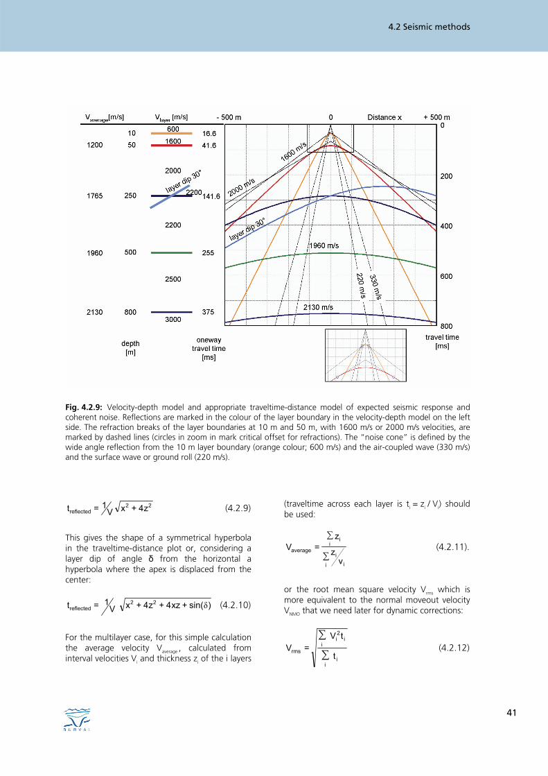
Fig. 4.2.9: Velocity-depth model and appropriate traveltime-distance model of expected seismic response and coherent noise. Reflections are marked in the colour of the layer boundary in the velocity-depth model on the left side. The refraction breaks of the layer boundaries at 10 m and 50 m, with 1600 m/s or 2000 m/s velocities, are marked by dashed lines (circles in zoom in mark critical offset for refractions). The “noise cone” is defined by the wide angle reflection from the 10 m layer boundary (orange colour; 600 m/s) and the air-coupled wave (330 m/s) and the surface wave or ground roll (220 m/s).

22reflected z4+xV

1=t (4.2.9)

This gives the shape of a symmetrical hyperbola in the traveltime-distance plot or, considering a layer dip of angle δ from the horizontal a hyperbola where the apex is displaced from the center:

)sin(+xz4+z4+xV1=t 22

reflected δ (4.2.10)

For the multilayer case, for this simple calculation the average velocity Vaverage , calculated from interval velocities Vi and thickness zi of the i layers

(traveltime across each layer is ti = zi / Vi) should be used:

∑

∑

i ii

ii

average

vz

z=V (4.2.11).

or the root mean square velocity Vrms which is more equivalent to the normal moveout velocity VNMO that we need later for dynamic corrections:

∑

∑

ii

ii

2i

rmst

tV=V (4.2.12)

HELGA WIEDERHOLD

42

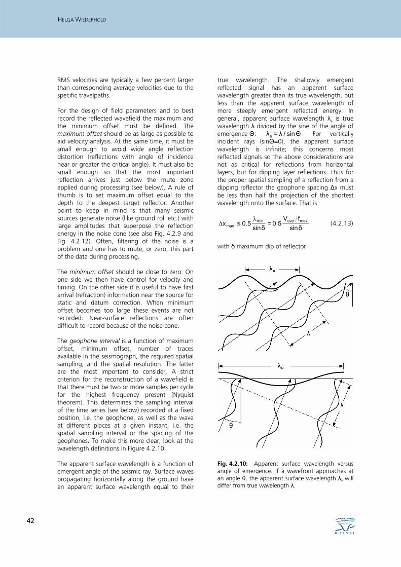
RMS velocities are typically a few percent larger than corresponding average velocities due to the specific travelpaths. For the design of field parameters and to best record the reflected wavefield the maximum and the minimum offset must be defined. The maximum offset should be as large as possible to aid velocity analysis. At the same time, it must be small enough to avoid wide angle reflection distortion (reflections with angle of incidence near or greater the critical angle). It must also be small enough so that the most important reflection arrives just below the mute zone applied during processing (see below). A rule of thumb is to set maximum offset equal to the depth to the deepest target reflector. Another point to keep in mind is that many seismic sources generate noise (like ground roll etc.) with large amplitudes that superpose the reflection energy in the noise cone (see also Fig. 4.2.9 and Fig. 4.2.12). Often, filtering of the noise is a problem and one has to mute, or zero, this part of the data during processing. The minimum offset should be close to zero. On one side we then have control for velocity and timing. On the other side it is useful to have first arrival (refraction) information near the source for static and datum correction. When minimum offset becomes too large these events are not recorded. Near-surface reflections are often difficult to record because of the noise cone. The geophone interval is a function of maximum offset, minimum offset, number of traces available in the seismograph, the required spatial sampling, and the spatial resolution. The latter are the most important to consider. A strict criterion for the reconstruction of a wavefield is that there must be two or more samples per cycle for the highest frequency present (Nyquist theorem). This determines the sampling interval of the time series (see below) recorded at a fixed position, i.e. the geophone, as well as the wave at different places at a given instant, i.e. the spatial sampling interval or the spacing of the geophones. To make this more clear, look at the wavelength definitions in Figure 4.2.10. The apparent surface wavelength is a function of emergent angle of the seismic ray. Surface waves propagating horizontally along the ground have an apparent surface wavelength equal to their

true wavelength. The shallowly emergent reflected signal has an apparent surface wavelength greater than its true wavelength, but less than the apparent surface wavelength of more steeply emergent reflected energy. In general, apparent surface wavelength λa is true wavelength λ divided by the sine of the angle of emergence Θ: Θsin/λ=λa . For vertically incident rays (sinΘ=0), the apparent surface wavelength is infinite; this concerns most reflected signals so the above considerations are not as critical for reflections from horizontal layers, but for dipping layer reflections. Thus for the proper spatial sampling of a reflection from a dipping reflector the geophone spacing Δx must be less than half the projection of the shortest wavelength onto the surface. That is

δsinfV

5.0=δsin

5.0≤x maxaveminmax

λΔ (4.2.13)

with δ maximum dip of reflector.

Fig. 4.2.10: Apparent surface wavelength versus angle of emergence. If a wavefront approaches at an angle θ, the apparent surface wavelength λa will differ from true wavelength λ.

4.2 Seismic methods

43

From the reflection signal point of view, another consideration in determining receiver interval involves the concept of the first Fresnel zone. Reflected energy represents a sampling from a relatively large area of the reflecting surface and this is related to the first Fresnel zone. The size and shape of the first Fresnel zone depend upon reflector depth z and wavelength λ of the reflected energy:

fT

V5.0=2

z=R 0λ

(4.2.14)

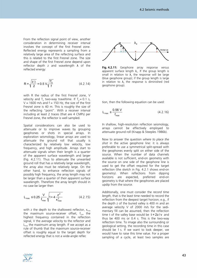
with R the radius of the first Fresnel zone, V velocity and T0 two-way traveltime. If T0 = 0.1 s, V = 1600 m/s and f = 150 Hz, the size of the first Fresnel zone is 40 m. This is roughly the size of the reflecting “point”. With a receiver interval including at least 2 traces (that are 4 CMPs) per Fresnel zone, the reflector is well sampled. Spatial considerations can also be used to attenuate or to improve waves by grouping geophones or shots in special arrays. In exploration seismology, linear arrays are used to attenuate the ground roll that usually is characterized by relatively low velocity, low frequency, and high amplitude. Arrays start to attenuate signals when their length is a quarter of the apparent surface wavelength and larger (Fig. 4.2.11). Thus to attenuate the unwanted ground roll that has a relatively large wavelength, the array also must be relatively large. On the other hand, to enhance reflection signals of possibly high frequency, the array length may not be larger than a quarter of their apparent surface wavelength. Therefore the array length should in no case be larger then

2max

2

maxmax x

z4+1

fV

25.0≤L (4.2.15)

with z the depth to the shallowest reflector, xmax the maximum source-receiver offset, fmax the highest frequency contained in the reflection signal, V the average velocity to the reflector and Lmax the maximuim array length. If we accept as a rule of thumb that the maximum source-receiver offset is roughly equal to the target depth for reflected energy that is not a wide-angle reflec

Fig. 4.2.11: Geophone array response versus apparent surface length λa. If the group length is small in relation to λa the response will be large (blue geophone group); if the group length is large in relation to λa the response is diminished (red geophone group).

tion, then the following equation can be used:

maxmax f

V56.0≤L (4.2.16)

In shallow, high-resolution reflection seismology, arrays cannot be effectively employed to attenuate ground roll (Knapp & Steeples 1986b). Now to answer the question where to place the shot in the active geophone line: it is always preferable to use a symmetrical split-spread with the geophones evenly split on either side of the source. When the number of data channels available is not sufficient, end-on geometry with the source on one side of the geophone line is used to get the offset required for the target reflection (the sketch in Fig. 4.2.1 shows end-on geometry). When reflections from dipping horizons are expected, preferred end-on geometry is that where the geophones are placed updip from the source. Additionally, one must consider the record time length, that is the least time needed to record the reflection from the deepest target horizon; e.g., if the depth z of the buried valley is 400 m and an average velocity V of 2000 m/s for the sedi-mentary fill can be assumed, then the reflection time t of the valley base would be v/z2=t and thus be 400 ms or 0.4 s. This is the two-way reflection time. To image also the surrounding or geological setting, the recording time in this case should be 1 s. If we want to look deeper, we would have to raise this time value. For a proper sampling of a cycle, at least two samples are

HELGA WIEDERHOLD

44

necessary. Expressed in relation to frequency, this means that the highest frequency that can be resolved, the Nyquist frequency fNy, needs the time between two sample points or sampling interval to be Nyf2/1=tΔ with Δt in milliseconds (ms) and f in hertz (Hz). In practice, four samples are recommended, or Nyf4/1=tΔ . Example: with a sampling interval of 1 ms, frequencies up to 250 Hz are well sampled; the Nyquist frequency is 500 Hz. To avoid aliasing, frequencies above the Nyquist frequency must be removed before sampling. The inverse of the sample interval is called sample rate ( tΔ1= ). 4.2.4 Data processing

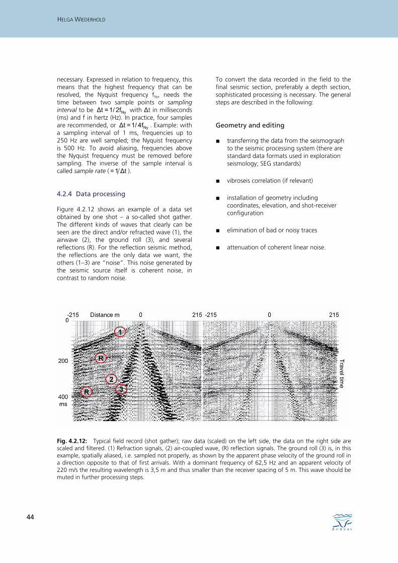
Figure 4.2.12 shows an example of a data set obtained by one shot – a so-called shot gather. The different kinds of waves that clearly can be seen are the direct and/or refracted wave (1), the airwave (2), the ground roll (3), and several reflections (R). For the reflection seismic method, the reflections are the only data we want, the others (1–3) are “noise”. This noise generated by the seismic source itself is coherent noise, in contrast to random noise.

To convert the data recorded in the field to the final seismic section, preferably a depth section, sophisticated processing is necessary. The general steps are described in the following: Geometry and editing

■ transferring the data from the seismograph to the seismic processing system (there are standard data formats used in exploration seismology; SEG standards)

■ vibroseis correlation (if relevant)

■ installation of geometry including coordinates, elevation, and shot-receiver configuration

■ elimination of bad or noisy traces

■ attenuation of coherent linear noise.

Fig. 4.2.12: Typical field record (shot gather); raw data (scaled) on the left side, the data on the right side are scaled and filtered. (1) Refraction signals, (2) air-coupled wave, (R) reflection signals. The ground roll (3) is, in this example, spatially aliased, i.e. sampled not properly, as shown by the apparent phase velocity of the ground roll in a direction opposite to that of first arrivals. With a dominant frequency of 62,5 Hz and an apparent velocity of 220 m/s the resulting wavelength is 3,5 m and thus smaller than the receiver spacing of 5 m. This wave should be muted in further processing steps.

4.2 Seismic methods

45

Signal enhancement (scaling, filtering, muting)

If we would look at the raw shot gather without any scaling, we would clearly see the decrease of amplitudes with distance and time. The earth has two effects on a propagating wavefield: (1) energy density decays proportionately to 1/r2 where r is the radius of the wavefront. Wave amplitude then, being proportional to the square root of energy density, decays with 1/r. As velocity usually increases with depth, this causes further divergence of the wavefront and a more rapid decay in amplitudes with distance. (2) The frequency content of the initial source signal changes in a time-variant manner as it propagates. In particular, high frequencies are absorbed more rapidly than low frequencies (due to intrinsic attenuation). These effects must be compensated by a time-variant scaling. By a time-invariant scaling, the amplitudes for each trace may be scaled or balanced with regard to the gather or individually. Also, automatic gain functions like AGC can be applied, but be aware that the true amplitude information is lost. Typically, prestack deconvolution (inverse filtering, spectral whitening, shaping the amplitude-frequency response) is aimed at improving temporal resolution by compressing the effective source wavelet contained in the seismic trace to a spike. After deconvolution, a wide band-pass filter is often needed. In the extreme case that ground roll is not attenuated or eliminated after the above processes, this area of the shot gather should be muted (zeroing the amplitudes) (Fig. 4.2.12). Travel time corrections (static corrections, dynamic corrections)

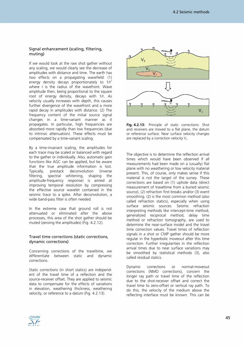
Concerning corrections of the traveltime, we differentiate between static and dynamic corrections. Static corrections (in short statics) are independ-ent of the travel time of a reflection and the source-receiver offset. They are applied to seismic data to compensate for the effects of variations in elevation, weathering thickness, weathering velocity, or reference to a datum (Fig. 4.2.13).

Fig. 4.2.13: Principle of static corrections: Shot and receivers are moved to a flat plane, the datum or reference surface. Near surface velocity changes are replaced by a correction velocity Vc.

The objective is to determine the reflection arrival times which would have been observed if all measurements had been made on a (usually) flat plane with no weathering or low velocity material present. This, of course, only makes sense if this material is not the target of the survey. These corrections are based on (1) uphole data (direct measurement of traveltime from a buried seismic source), (2) refraction first breaks and/or (3) event smoothing. (2) is the most common method (also called refraction statics), especially when using surface seismic sources. Seismic refraction interpreting methods like intercept-time method, generalized reciprocal method, delay time method or refraction tomography, are used to determine the near-surface model and the travel time correction values. Travel times of reflection signals in a shot or CMP gather should be more regular in the hyperbolic moveout after this time correction. Further irregularities in the reflection arrival times due to near surface variations may be smoothed by statistical methods (3), also called residual statics. Dynamic corrections or normal-moveout corrections (NMO corrections), concern the longer ray path or travel time of the reflection due to the shot-receiver offset and correct the travel time to zero-offset or vertical ray path. To do this, the velocity of the medium above the reflecting interface must be known. This can be

HELGA WIEDERHOLD

46

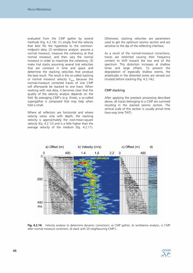
evaluated from the CMP gather by several methods (Fig. 4.2.14): (1) simply find the velocity that best fits the hyperbola to the common-midpoint data; (2) semblance analysis: assume a normal moveout, measure the coherency at that normal moveout, and then vary the normal moveout in order to maximize the coherency; (3) make trial stacks assuming several trial velocities that are constant in time and space and determine the stacking velocities that produce the best result. The result is the so-called stacking or normal moveout velocity VNMO because the normal-moveout corrected traces of one CMP will afterwards be stacked to one trace. When working with real data, it becomes clear that the quality of the velocity analysis depends on the fold. By averaging CMP’s (e.g. three), a so-called supergather is composed that may help when fold is small. Where all reflectors are horizontal and where velocity varies only with depth, the stacking velocity is approximately the root-mean-square velocity (Eq. 4.2.12) and is a little higher than the average velocity of the medium (Eq. 4.2.11).

Otherwise, stacking velocities are parameters used to get the optimum seismic section and are sensitive to the dip of the reflecting interface. As a result of the normal-moveout corrections, traces are stretched causing their frequency content to shift toward the low end of the spectrum. This distortion increases at shallow times and large offsets. To prevent the degradation of especially shallow events, the amplitudes in the distorted zones are zeroed out (muted) before stacking (Fig. 4.2.14c). CMP stacking

After applying the prestack processing described above, all traces belonging to a CMP are summed resulting in the stacked seismic section. The vertical scale of this section is usually arrival time (two-way time TWT).

Fig. 4.2.14: Velocity analysis to determine dynamic corrections: a) CMP gather, b) semblance analysis, c) CMP after normal moveout correction, d) stack with 20 neighbouring CMP’s.

4.2 Seismic methods

47

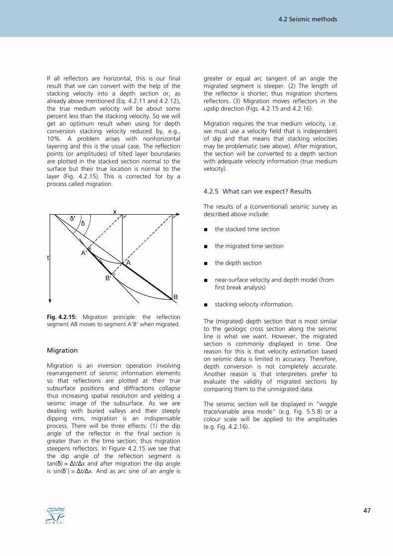
If all reflectors are horizontal, this is our final result that we can convert with the help of the stacking velocity into a depth section or, as already above mentioned (Eq. 4.2.11 and 4.2.12), the true medium velocity will be about some percent less than the stacking velocity. So we will get an optimum result when using for depth conversion stacking velocity reduced by, e.g., 10%. A problem arises with nonhorizontal layering and this is the usual case. The reflection points (or amplitudes) of tilted layer boundaries are plotted in the stacked section normal to the surface but their true location is normal to the layer (Fig. 4.2.15). This is corrected for by a process called migration.

Fig. 4.2.15: Migration principle: the reflection segment AB moves to segment A’B’ when migrated.

Migration

Migration is an inversion operation involving rearrangement of seismic information elements so that reflections are plotted at their true subsurface positions and diffractions collapse thus increasing spatial resolution and yielding a seismic image of the subsurface. As we are dealing with buried valleys and their steeply dipping rims, migration is an indispensable process. There will be three effects: (1) the dip angle of the reflector in the final section is greater than in the time section; thus migration steepens reflectors. In Figure 4.2.15 we see that the dip angle of the reflection segment is tan(δ) = Δt/Δx and after migration the dip angle is sin(δ’) = Δt/Δx. And as arc sine of an angle is

greater or equal arc tangent of an angle the migrated segment is steeper. (2) The length of the reflector is shorter; thus migration shortens reflectors. (3) Migration moves reflectors in the updip direction (Figs. 4.2.15 and 4.2.16). Migration requires the true medium velocity, i.e. we must use a velocity field that is independent of dip and that means that stacking velocities may be problematic (see above). After migration, the section will be converted to a depth section with adequate velocity information (true medium velocity). 4.2.5 What can we expect? Results

The results of a (conventional) seismic survey as described above include: ■ the stacked time section

■ the migrated time section

■ the depth section

■ near-surface velocity and depth model (from first break analysis)

■ stacking velocity information.

The (migrated) depth section that is most similar to the geologic cross section along the seismic line is what we want. However, the migrated section is commonly displayed in time. One reason for this is that velocity estimation based on seismic data is limited in accuracy. Therefore, depth conversion is not completely accurate. Another reason is that interpreters prefer to evaluate the validity of migrated sections by comparing them to the unmigrated data. The seismic section will be displayed in “wiggle trace/variable area mode” (e.g. Fig. 5.5.8) or a colour scale will be applied to the amplitudes (e.g. Fig. 4.2.16).

HELGA WIEDERHOLD

48

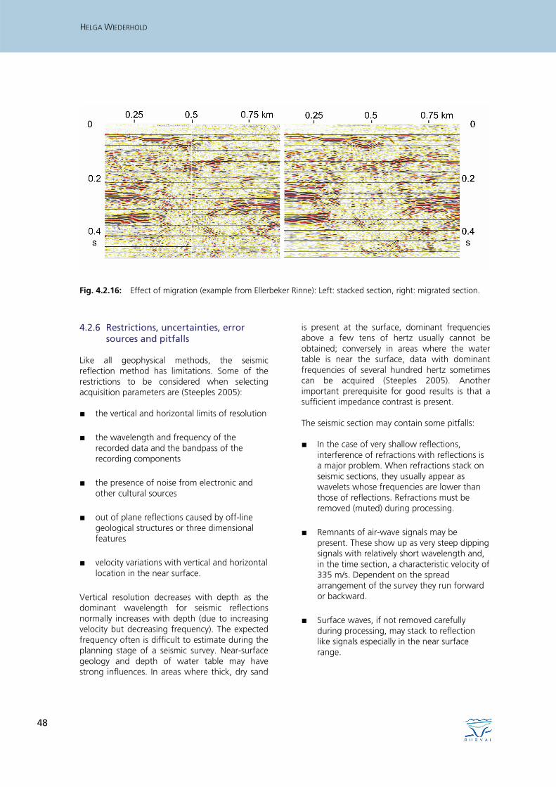
Fig. 4.2.16: Effect of migration (example from Ellerbeker Rinne): Left: stacked section, right: migrated section.

4.2.6 Restrictions, uncertainties, error

sources and pitfalls

Like all geophysical methods, the seismic reflection method has limitations. Some of the restrictions to be considered when selecting acquisition parameters are (Steeples 2005): ■ the vertical and horizontal limits of resolution

■ the wavelength and frequency of the recorded data and the bandpass of the recording components

■ the presence of noise from electronic and other cultural sources

■ out of plane reflections caused by off-line geological structures or three dimensional features

■ velocity variations with vertical and horizontal location in the near surface.

Vertical resolution decreases with depth as the dominant wavelength for seismic reflections normally increases with depth (due to increasing velocity but decreasing frequency). The expected frequency often is difficult to estimate during the planning stage of a seismic survey. Near-surface geology and depth of water table may have strong influences. In areas where thick, dry sand

is present at the surface, dominant frequencies above a few tens of hertz usually cannot be obtained; conversely in areas where the water table is near the surface, data with dominant frequencies of several hundred hertz sometimes can be acquired (Steeples 2005). Another important prerequisite for good results is that a sufficient impedance contrast is present. The seismic section may contain some pitfalls: ■ In the case of very shallow reflections,

interference of refractions with reflections is a major problem. When refractions stack on seismic sections, they usually appear as wavelets whose frequencies are lower than those of reflections. Refractions must be removed (muted) during processing.

■ Remnants of air-wave signals may be present. These show up as very steep dipping signals with relatively short wavelength and, in the time section, a characteristic velocity of 335 m/s. Dependent on the spread arrangement of the survey they run forward or backward.

■ Surface waves, if not removed carefully during processing, may stack to reflection like signals especially in the near surface range.

4.2 Seismic methods

49

■ Migration effects, i.e., if velocities higher than the actual medium velocity are used for migration typical “smiles” may occur. If we use too low velocities there may be remnants of diffractions.

■ Multiples, that is seismic energy which has been reflected more than once, are identified by their travel times, and/or may be identified during velocity analysis by their velocity. Multiples are not a severe problem of onshore near surface seismic data.

Principally, to validate a seismic section and their conclusions, interpreters must have access to at least one field file, along with display copies of one or more of the intermediate processing steps whenever possible (Steeples & Miller 1998). Vertical seismic profiles allow the accurate determination of the travel time of seismic waves to various geologic units and thus allow the accurate determination of seismic velocities. They are recommended to secure depth sections and interpretations. 4.2.7 References

Buness AH, Druivenga G, Wiederhold H (2000): SISSY – eine tragbare und leistungsstarke seismische Energiequelle. – Geol. JB. E52: 63–88.

Gabriel G, Kirsch R, Siemon B, Wiederhold H (2003): Geophysical investigation of buried Pleistocene subglacial valleys in Northern Germany. – Journal of Applied Geophysics 53: 159–180.

Knapp RW, Steeples DW (1986a): High-resolution common-depth-point seismic reflection profiling – Instrumentation. – Geophysics 51: 276–282.

Knapp RW, Steeples DW (1986b): High-resolution common-depth-point reflection profiling – Field acquisition parameter design. – Geophysics 51: 283–294.

Knödel K, Krummel H, Lange G (1997): Geophysik. – Handbuch zur Erkundung des Untergrundes von Deponien und Altlasten Band 3, Springer; Berlin Heidelberg.

Pelton JR (2005): Near-Surface Seismology: Surface-Based Methods. – In: Butler DK (Ed.), Near-Surface Geophysics: 219–264, Soc. of Expl. Geophys.; Tulsa, USA.

Rabbel W (2006): Seismic methods. – In: Kirsch R (Ed.), Groundwater geophysics – A tool for hydrogeology: 23–84; Springer; Berlin Heidelberg.

Sheriff RE (2002): Encyclopedic Dictionary of Exploration Geophysics (4th ed.). – Soc. of Expl. Geophys.; Tulsa, USA.

Steeples DW (2005): Shallow seismic methods. – In: Rubin Y, Hubbard SS (Eds.), Hydrogeophysics: 215–251, Springer; Dordrecht, the Netherlands.

Steeples DW, Miller RD (1998): Avoiding pitfalls in shallow seismic reflection surveys. Geophysics 63: 1213–1224.

Steeples DW, Green AG, McEvilly TV, Miller RD, Doll WE, Rector JW (1997): A workshop examination of shallow seismic reflection surveying. – The Leading Edge 16: 1641–1647.

Wiederhold H, Gabriel G, Grinat M (2005): Geophysikalische Erkundung der Bremer-haven-Cuxhavener Rinne im Umfeld der Forschungsbohrung Cuxhaven. – Z. Angew. Geol. 51(1): 28–38.

Yilmaz O (2001): Seismic Data Analysis (vol 1 and 2, 2nd ed.). – Soc. of Expl. Geophys.; Tulsa, USA.

HELGA WIEDERHOLD

50

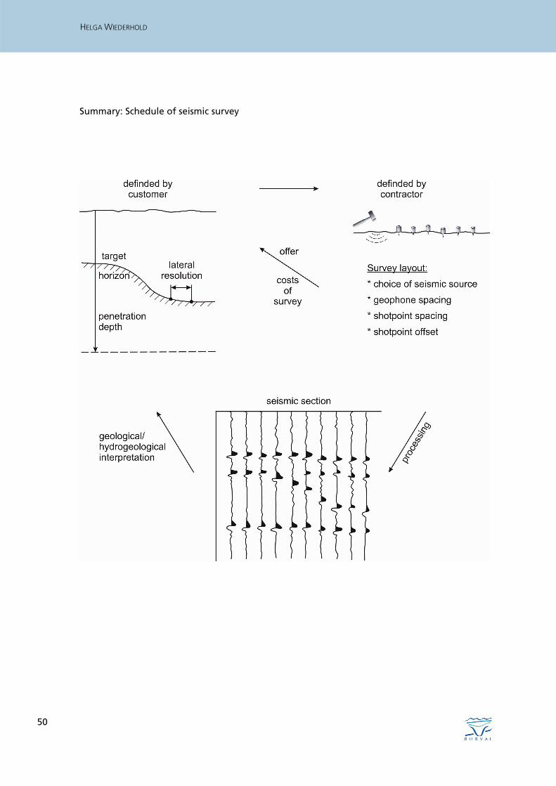
Summary: Schedule of seismic survey