© 2012 EAGE www.firstbreak.org 39

special topicfirst break volume 30, March 2012

Modelling/Interpretation

1 Roxar Software Solutions, Emerson Process Management.2 Norwegian Computing Centre.* Corresponding author, E-mail:

Seismic Inversion and its Applications in Reservoir Characterization

Krishnakumar Narayanan Nair,1 Odd Kolbjørnsen,2 and Arne Skaorstad,1 review seismic inversion and propose a fast and efficient way of estimating elastic properties and facies proba-bility parameters using the results from inversion and through the incorporation of facies logs.

W hile seismic inversion is successful in estimat-ing the elastic properties from seismic data with greater vertical resolution and acceptable noise levels, Bayesian inversion methodology is able to

provide an assessment of uncertainty which brings value to the geomodeller.

The primary goal of this article will be to illustrate the application of inverted parameters for reservoir modelling. Reservoir modellers often use seismic attributes from band limited input seismic data to condition facies and petrophysi-cal models. However, such band-limited seismic data doesn’t capture the low and high frequency information, due to the earth’s filtering, and it is usually difficult to capture the minute details of the reservoir properties, due to the lack of low frequency contents in the seismic data.

The suggested alternative is to use elastic properties as well as facies probability parameters to condition property models for improved volumetric estimation. The result will be higher quality and more accurate reservoir models. In addition, the facies probability parameters generated using inversion can assist the geomodeller to guide facies simulation.

Simultaneous geostatistical inversionIt is assumed that seismic data is generated as a result of the wavelet convolution with Earth’s reflectivity series. The reflec-tivity series is considered to be a function of elastic properties and, hence, the reverse process of estimating elastic properties from the observed seismic data is known as inverse modelling.

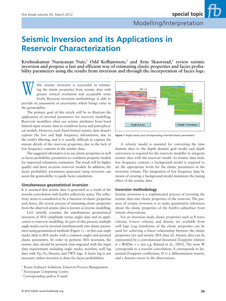
Let’s initially examine the simultaneous geostatistical inversion of AVA (amplitude versus angle) data and its appli-cation to reservoir modelling. As part of this process, multiple angle stacks can be inverted simultaneously into elastic param-eters using geostatistical methods (Figure 1) – in this case angle stacks (that is AVA stacks with a common angle) and inverted elastic parameters. In order to perform AVA inversion, the seismic data should be prestack time migrated with the input data requirements including angle stacks, wavelets, well log data with Vp, Vs, Density, and TWT logs. A facies log is not necessary unless inversion is done for facies probabilities.

A velocity model is essential for converting the time domain data to the depth domain grid model and depth conversion is required for the reservoir modeller to integrate seismic data with the reservoir model. As seismic data lacks low frequency content, a background model is required to set the appropriate levels for the elastic parameters in the inversion volume. The integration of low frequency data by means of creating a background model minimizes the tuning effect of the seismic data.

Inversion methodologySeismic inversion is a sophisticated process of inverting the seismic data into elastic properties of the reservoir. The pur-pose of seismic inversion is to make quantitative inferences about the elastic properties of the Earth’s subsurface from remote observations.

For an inversion study, elastic properties such as P-wave velocity, S-wave velocity, and density are available from well logs. Log transforms of the elastic properties can be used for achieving a linear relationship between the elastic properties (m) and seismic AVA data (d). Seismic data can be represented by a convolutional linearized Zoeppritz relation d = WADm + e (see e.g. Buland et al., 2003). The term W corresponds to a wavelet convolution, A corresponds to lin-earized Zoeppritz coefficients, D is a differentiation matrix, and e denotes errors in the observations.

Figure 1 Angle stacks and corresponding inverted elastic parameters.

www.firstbreak.org © 2012 EAGE40

special topic first break volume 30, March 2012

Modelling/Interpretation

In order to create a background model, the first step is to estimate a vertical trend from the well logs. Before estimating the vertical trend, it is mandatory to check the alignment of the wells. If time surfaces are available, that can be used for controlling the alignment. It is also important that the align-ment reflects the correlation structure (deposition/compaction).

The trend extraction starts by calculating an average log value for each layer. This average is calculated for the Vp, Vs, and Rho well logs and is based on all available wells. When the inversion volume has been filled with the vertical time trend, it can be filtered to low frequencies which are absent in the seismic data. Kriging is used to ensure that the back-ground model matches the well data. Ideally, the background model should be as smooth as possible.

As with the prior model for the elastic parameters, a full time dependant error covariance matrix is collapsed into a noise covariance matrix, a lateral correlation vector and a temporal correlation vector. The lateral correlation is usually difficult to estimate and one choice is to make it equal to that of the elastic parameters. The temporal correlation can be partly estimated from well tie analysis.

A noise estimate can be found by generating synthetic seismic data using the wavelet optimally shifted in each well, and subtracting this from the seismic data. The remaining part can be assumed to be noise, and we can then measure the noise energy from this. The correlation between the noises in different angle stacks is hard to estimate but can be included through a parametric model.

Wavelets can be estimated at all well locations, where we obtain the reflection coefficients from well logs. The standard seismic convolution equation can be written as d = w*c + e, where d is the seismic amplitude data, w is the wavelet, c the reflection coefficients and e is the noise.

This will be transferred to the Fourier domain and multiplied with the reflection coefficients. Solving this in the frequency domain is unstable, so it is advisable to conduct smoothing. This is possible by transforming back to the time domain, multiplying with a Papoulis taper, and transforming them back to the frequency domain (White, R.E., and Simm, R., 1998).

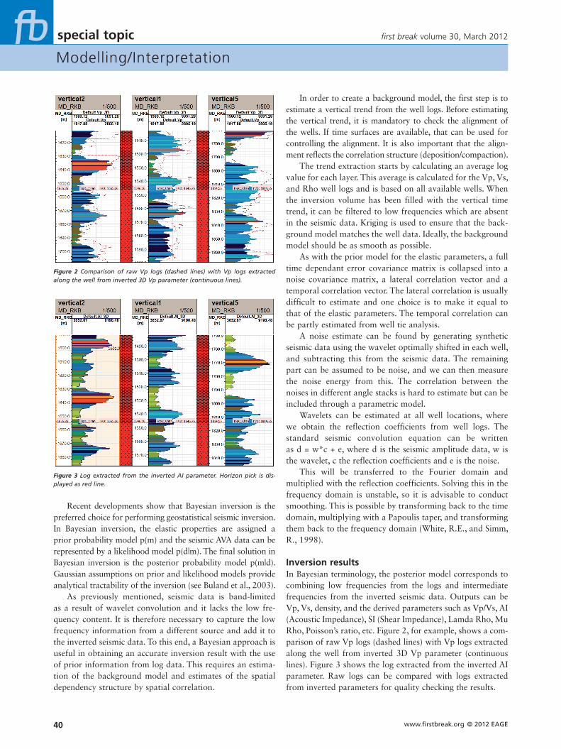
Inversion resultsIn Bayesian terminology, the posterior model corresponds to combining low frequencies from the logs and intermediate frequencies from the inverted seismic data. Outputs can be Vp, Vs, density, and the derived parameters such as Vp/Vs, AI (Acoustic Impedance), SI (Shear Impedance), Lamda Rho, Mu Rho, Poisson’s ratio, etc. Figure 2, for example, shows a com-parison of raw Vp logs (dashed lines) with Vp logs extracted along the well from inverted 3D Vp parameter (continuous lines). Figure 3 shows the log extracted from the inverted AI parameter. Raw logs can be compared with logs extracted from inverted parameters for quality checking the results.

Recent developments show that Bayesian inversion is the preferred choice for performing geostatistical seismic inversion. In Bayesian inversion, the elastic properties are assigned a prior probability model p(m) and the seismic AVA data can be represented by a likelihood model p(d|m). The final solution in Bayesian inversion is the posterior probability model p(m|d). Gaussian assumptions on prior and likelihood models provide analytical tractability of the inversion (see Buland et al., 2003).

As previously mentioned, seismic data is band-limited as a result of wavelet convolution and it lacks the low fre-quency content. It is therefore necessary to capture the low frequency information from a different source and add it to the inverted seismic data. To this end, a Bayesian approach is useful in obtaining an accurate inversion result with the use of prior information from log data. This requires an estima-tion of the background model and estimates of the spatial dependency structure by spatial correlation.

Figure 2 Comparison of raw Vp logs (dashed lines) with Vp logs extracted along the well from inverted 3D Vp parameter (continuous lines).

Figure 3 Log extracted from the inverted AI parameter. Horizon pick is dis-played as red line.

© 2012 EAGE www.firstbreak.org 41

special topicfirst break volume 30, March 2012

Modelling/Interpretation

Accuracy can be achieved by the calibration of seismic data to information observed at wells.

Geoscientists are required to make sure that the time to depth conversion and seismic-well tie has been performed accurately. To this end, inverted seismic data can guide the distribution of petrophysical properties such as porosity or water saturation. The calibration of seismic information is often difficult for various reasons, such as scale difference between seismic, modelling grid cell size and well data, and the inability of the seismic data to clearly discriminate between petrophysical variations across the reservoir.

These issues can be over-ridden to a certain extent with the use of prior information used in inversion from the well logs. With reservoir modelling, the goal of inversion is to extract acoustic properties that are highly correlated with

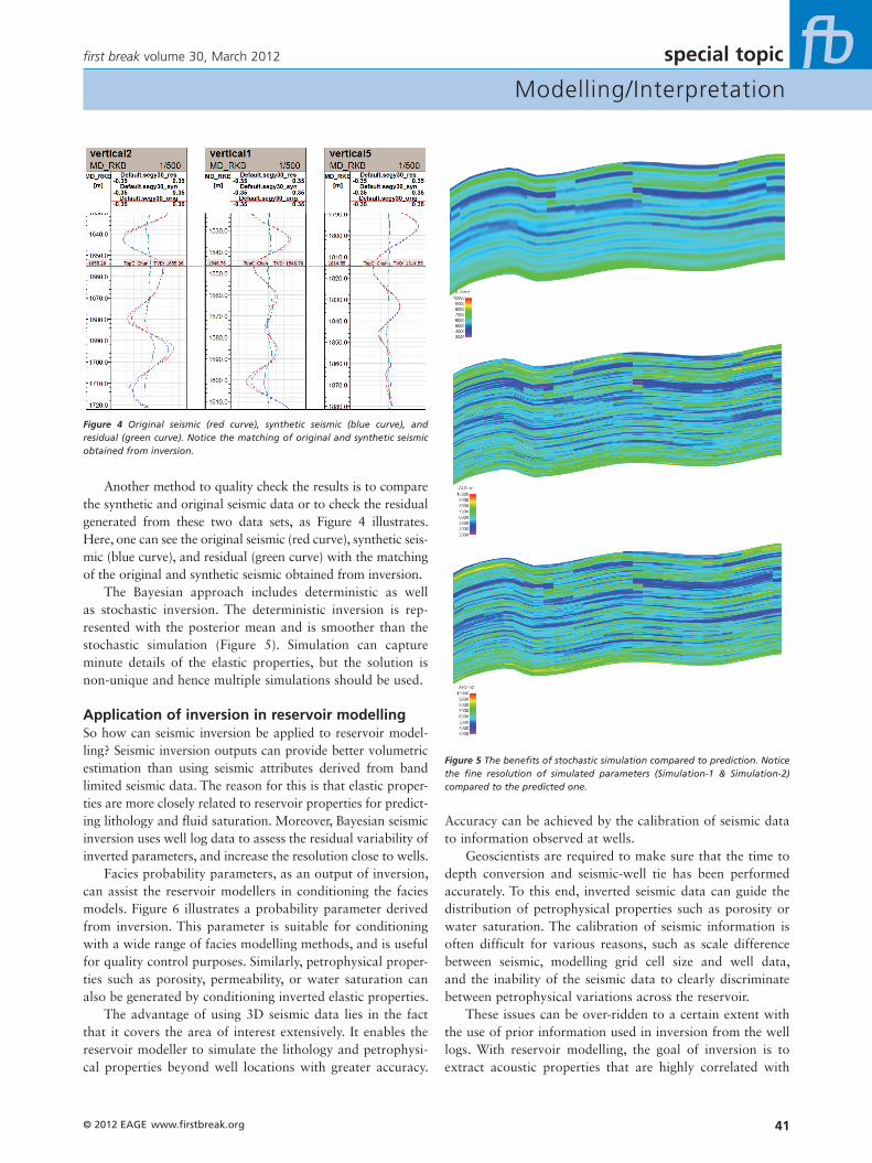
Another method to quality check the results is to compare the synthetic and original seismic data or to check the residual generated from these two data sets, as Figure 4 illustrates. Here, one can see the original seismic (red curve), synthetic seis-mic (blue curve), and residual (green curve) with the matching of the original and synthetic seismic obtained from inversion.

The Bayesian approach includes deterministic as well as stochastic inversion. The deterministic inversion is rep-resented with the posterior mean and is smoother than the stochastic simulation (Figure 5). Simulation can capture minute details of the elastic properties, but the solution is non-unique and hence multiple simulations should be used.

Application of inversion in reservoir modellingSo how can seismic inversion be applied to reservoir model-ling? Seismic inversion outputs can provide better volumetric estimation than using seismic attributes derived from band limited seismic data. The reason for this is that elastic proper-ties are more closely related to reservoir properties for predict-ing lithology and fluid saturation. Moreover, Bayesian seismic inversion uses well log data to assess the residual variability of inverted parameters, and increase the resolution close to wells.

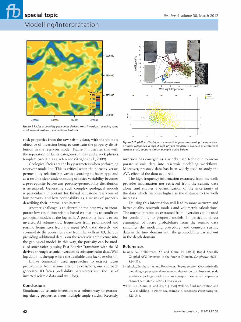
Facies probability parameters, as an output of inversion, can assist the reservoir modellers in conditioning the facies models. Figure 6 illustrates a probability parameter derived from inversion. This parameter is suitable for conditioning with a wide range of facies modelling methods, and is useful for quality control purposes. Similarly, petrophysical proper-ties such as porosity, permeability, or water saturation can also be generated by conditioning inverted elastic properties.

The advantage of using 3D seismic data lies in the fact that it covers the area of interest extensively. It enables the reservoir modeller to simulate the lithology and petrophysi-cal properties beyond well locations with greater accuracy.

Figure 4 Original seismic (red curve), synthetic seismic (blue curve), and residual (green curve). Notice the matching of original and synthetic seismic obtained from inversion.

Figure 5 The benefits of stochastic simulation compared to prediction. Notice the fine resolution of simulated parameters (Simulation-1 & Simulation-2) compared to the predicted one.

www.firstbreak.org © 2012 EAGE42

special topic first break volume 30, March 2012

Modelling/Interpretation

inversion has emerged as a widely used technique to incor-porate seismic data into reservoir modelling workflows. Moreover, prestack data has been widely used to study the AVA effect of the data acquired.

The high frequency information extracted from the wells provides information not retrieved from the seismic data alone, and enables a quantification of the uncertainty of the data which becomes higher as the distance to the wells increases.

Utilizing this information will lead to more accurate and better quality reservoir models and volumetric calculations. The output parameters extracted from inversion can be used for conditioning to property models. In particular, direct estimation of facies probabilities from the seismic data simplifies the modelling procedure, and connects seismic data in the time domain with the geomodelling carried out in the depth domain.

ReferencesBuland, A., Kolbjornsen, O. and Omre, H. [2003] Rapid Spatially

Coupled AVO Inversion in the Fourier Domain. Geophysics, 68(1),

824–836.

Stright, L., Bernhardt, A. and Boucher, A. [In preparation] Geostatistically

modelling topographically-controlled deposition of sub-seismic scale

sandstone packages within a mass transport dominated deep-water

channel belt. Mathematical Geosciences.

White, R.E., Simm, R. and Xu, S. [1998] Well tie, fluid substitution and

AVO modelling - a North Sea example. Geophysical Prospecting 46,

323–346.

rock properties from the raw seismic data, with the ultimate objective of inversion being to constrain the property distri-bution in the reservoir model. Figure 7 illustrates this with the separation of facies categories in logs and a rock physics template overlain as a reference (Stright et al., 2009).

Geological facies are the key parameters when performing reservoir modelling. This is critical when the porosity versus permeability relationship varies according to facies type and as a result a clear understanding of facies variability becomes a pre-requisite before any porosity-permeability distribution is attempted. Generating such complex geological models is particularly important for fluvial sandstone reservoirs of low porosity and low permeability as a means of properly describing their internal architecture.

Another challenge is to determine the best way to incor-porate low resolution seismic based estimations to condition geological models at the log scale. A possibility here is to use inverted AI volume (low frequencies from prior model and seismic frequencies from the input AVA data) directly and co-simulate the porosities away from the wells in 3D, thereby providing additional details on the reservoir architecture into the geological model. In this way, the porosity can be mod-elled stochastically using Fast Fourier Transform with the AI derived through seismic inversion as soft constraint data. Well log data fills the gap where the available data lacks resolution.

Unlike commonly used approaches to extract facies probabilities from seismic attribute crossplots, our approach generates 3D facies probability parameters with the use of inverted seismic data and well logs.

ConclusionsSimultaneous seismic inversion is a robust way of extract-ing elastic properties from multiple angle stacks. Recently,

Figure 6 Facies probability parameter derived from inversion, revealing some predominant east-west channelized features.

Figure 7 (Top) Plot of Vp/Vs versus acoustic impedance showing the separation of facies categories in logs. A rock physics template is overlain as a reference (Stright et al., 2009). A similar example is also below.