seismic interferometry, surface waves and source distribution · seismic interferometry, surface...

Geophys. J. Int. (2008) 175, 1067–1087 doi: 10.1111/j.1365-246X.2008.03918.x

GJI

Sei

smol

ogy

Seismic interferometry, surface waves and source distribution

David Halliday∗ and Andrew Curtis∗School of GeoSciences, Institute of Earth Science, The University of Edinburgh, UK. E-mail: [email protected]

Accepted 2008 July 14. Received 2008 June 26; in original form 2007 October 18

S U M M A R YSeismic interferometry can be used to estimate interreceiver surface wave signals by cross-correlation of signals recorded at each receiver. The quality of the estimated surface wavesis controlled by the distribution of sources exciting the cross-correlated wavefields, and it iscommonly thought that only sources at or near the surface are required to generate accurateestimates. We study the role of source distribution in surface wave interferometry for bothsurface and subsurface sources using surface wave Green’s functions for laterally homogeneousmedia. We solve the interferometric integral using a Rayleigh wave orthogonality relationshipcombined with a stationary phase approach. Contrary to popular opinion we find that sourcesat depth do indeed play a role in the recovery of surface waves by interferometry. We findthat interferometry performs well when surface sources are distributed homogeneously at thesurface of the Earth. However, when this homogeneous distribution is not available amplitudeerrors are introduced, and when multiple modes are present strong spurious events appear andhigher mode surface waves may not be correctly estimated. In order to recover higher modesurface waves we propose an additional step in the processing of surface wave data for seismicinterferometry: by separating modes and applying interferometry to each mode individually itis possible to recover the interreceiver surface wave modes, without the artefacts introducedby limited source coverage.

Key words: Interferometry; Surface waves and free oscillations; Theoretical seismology.

1 I N T RO D U C T I O N

In seismic interferometry Green’s functions between pairs of receivers are extracted by cross-correlation of wavefields recorded at eachreceiver that are excited by sources on a closed surface surrounding the receivers. The Green’s functions are the signals that would be recordedat one receiver if an impulsive point source was fired at the location of the other receiver. Thus, interferometry synthesizes the data that wouldhave been recorded if one of the receivers had been a source and the other had been a receiver (Lobkis & Weaver 2001; Weaver & Lobkis2001; Snieder 2004a; Wapenaar 2004; Wapenaar & Fokkema 2006).

These wavefields can be excited by active sources or passive sources, and applications of the method vary with details changing from caseto case (Curtis et al. 2006). For example, van Manen et al. (2005, 2006, 2007) propose an efficient full wavefield modelling algorithm basedon seismic interferometry. They extract the exact Green’s functions between any pair of points in a synthetic medium by cross-correlatingwavefields recorded at each point, arising from two different source types on an enclosing boundary. Bakulin & Calvert (2004, 2006) presenta related approach in which they use active sources on the surface of the Earth and cross-correlate recorded wavefields at pairs of receiversplaced in subsurface wells to simulate data from a subsurface source at one of the receiver locations. Draganov et al. (2007) apply passiveseismic interferometry by cross-correlating recordings of background noise in a desert setting to estimate interreceiver reflected wavefields.

A popular application of seismic interferometry is the isolation of interreceiver surface wave signals. When the sources used ininterferometry are located at or near the surface of the earth they predominantly excite surface waves that travel between the two receivers.For example, in exploration seismology, direct and scattered interreceiver surface waves can be estimated using active sources at the surface.The estimated surface waves can then be used as part of a source–receiver surface wave removal algorithm in order to expose the desired andmuch weaker body wave energy (Curtis et al. 2006; Dong et al. 2006; Halliday et al. 2007, 2008). In earthquake seismology interferometry isapplied to so-called passive wavefields emanating from unknown sources in or on the Earth (Shapiro & Campillo 2004; Shapiro et al. 2005),or from secondary scattering sources (as illustrated using the seismic coda by Campillo & Paul 2003). The resulting interreceiver seismograms

∗Also at: ECOSSE (Edinburgh Collaborative of Subsurface Science and Engineering), UK.

C© 2008 The Authors 1067Journal compilation C© 2008 RAS

1068 D. Halliday and A. Curtis

are dominated by fundamental mode Rayleigh waves and these are used to invert for group velocity maps (e.g. Gertstoft et al. 2006). Inengineering/near-surface seismology near-surface shear wave velocity profiles can be extracted from recordings of ambient noise (a processreferred to as microtremor analysis, e.g. Aki 1957; Louie 2001) and from active source surface wave recordings (Xia et al. 2000; Beaty et al.2002). Chavez-Garcıa & Luzon (2005) investigate the relationship between microtremor analysis and passive seismic interferometry andHalliday et al. (2008) illustrate that in a suburban environment interferometric surface wave estimates can be produced using both backgroundnoise sources (i.e. motorway traffic, building sites, main roads, etc.) and active sources (similar to the estimates used for ground roll removal).

Theory dictates that a closed surface of sources is required for seismic interferometry (e.g. Wapenaar & Fokkema 2006). The range ofapplications introduced above illustrate that this requirement may, in practise, be able to be relaxed. However, limited source coverage doesintroduce errors and it is important to understand these. For example, Snieder et al. (2006) use a stationary phase approach to show howspurious multiples are introduced when attempting to recover reflected body waves using only surface sources. As a consequence Mehta et al.(2007) use wavefield separation to suppress the contribution of such spurious events in an application of the virtual source method of Bakulin& Calvert (2004, 2006).

Here we study the effect of missing subsurface sources and different source distributions on the interferometric construction of surfacewaves. We use a stationary phase approach similar to Snieder (2004a), who uses a 2-D source distribution to show that interreceiver surfacewaves can be correctly recovered from recordings of passive noise fields when the sources of noise are distributed homogeneously at the surfaceof the Earth. We present a comprehensive 3-D analysis of the interferometric integral using surface wave Green’s functions, considering theeffects of source type, sources at depth, and in particular the effect on higher mode surface waves.

We conclude that: (1) contrary to commonly cited opinion, sources at depth play an important role in seismic interferometry for surfacewaves, particularly when we are interested in the construction of higher mode surface waves—without sources at depth we cannot expect toestimate higher mode surface waves correctly; (2) both point forces and deformation-rate-tensor sources are required to recover the correctrelative amplitudes of different surface wave modes; (3) when the homogeneous surface source distribution assumed by Snieder (2004a) is notpresent we can still recover good estimates of the correct interreceiver surface waves but only when individual modes can be isolated and (4)it is more difficult to recover correct multimode interreceiver surface waves due to the introduction of spurious events in the interferometricsynthesis.

The above conclusions do not prohibit interferometric higher-mode surface wave estimation. While amplitude errors are introducedit is still possible to recover the correct phase of the surface waves. The spurious events introduced in the presence of higher modes arecreated by the cross-correlations between different modes and may be avoided by separating the individual surface wave modes prior tointerferometry. We therefore, propose modal separation (where possible) prior to the application of seismic interferometry. Surface wavemodes can be separated using bandpass filters (Crampin & Bath 1965), phase matched filtering (Hwang & Mitchell 1986) or mode-branchstripping (van Heijst & Woodhouse 1997), but modes are more efficiently separated using frequency–wavenumber analysis, common inexploration geophysics where receiver arrays are well sampled spatially (e.g. Vermeer 2002). In earthquake seismology, densely sampledseismograph arrays are rare, however array methods still exist to identify and separate higher modes (e.g. Nolet 1975; Nolet & Panza 1976;Cara 1978; Mitchel 1980).

In exploration seismology our findings have implications for the prediction and removal of ground roll with interferometry. Ground rolloften consists of complex surface waves, exhibiting higher modes and multiple scattering (e.g. Al-Husseini et al. 1981; Herman & Perkins2006; Halliday et al. 2008). Hence, when only surface source geometries are available (as is the usual case in exploration seismology) modalseparation may be a key process in the application of seismic interferometry to such settings, as in order to remove higher modes correctlywe must be able to estimate these with the smallest possible error.

In earthquake seismology, our results explain why higher mode surface waves may not be recovered correctly, since the Earth’s passivenoise fields are predominantly excited by heterogeneous near-surface source distributions. To date, applications of interferometry at crustaland lithospheric scale only consider the recovery of fundamental mode surface waves (Gertstoft et al. 2006; Moschetti et al. 2007; Yanget al. 2007; Lin et al. 2008; Yao et al. 2008). While these surface waves produce velocity maps in agreement with regional geology, highermodes can be used to provide information in depth ranges unsampled by the fundamental mode (e.g. MacBeth & Burton 1985; Dost 1990;Yoshizawa & Kennet 2004). Thus the recovery of higher mode surface waves using modal separation may allow for improved velocity mapsfrom seismic interferometry. This argument also applies to applications of interferometry to near-surface engineering surveys, where highermode surface waves are commonly used to enhance the depth resolution of near-surface velocity models (e.g. Xia et al. 2000; Beaty et al.2002).

Finally, the methods used here may also be extended to body waves. Under certain circumstances the full elastic response of a systemcan be written as a sum of normal modes (Aki & Richards 2002, chap. 7; Snieder 2002). Therefore, an extension of this approach may allowfor detailed analysis of errors introduced by restricted source coverage in the body wave case, or for the analysis of the effect of body waveson surface wave interferometry.

In this paper, we first introduce the appropriate interferometric equations and surface wave Green’s functions and use a 2-D syntheticexample to illustrate the effect of using only surface sources in seismic interferometry. We then use the surface wave Green’s functionsto analyse the interferometric integral for surface waves. This analysis allows us to investigate the role of missing subsurface sources inmore detail and the effect of different surface source distributions. Finally, we discuss possible implications of our results and observations,providing possible solutions to allow for the recovery of higher mode surface waves in different applications of seismic interferometry.

C© 2008 The Authors, GJI, 175, 1067–1087

Journal compilation C© 2008 RAS

Seismic interferometry, surface waves and source distribution 1069

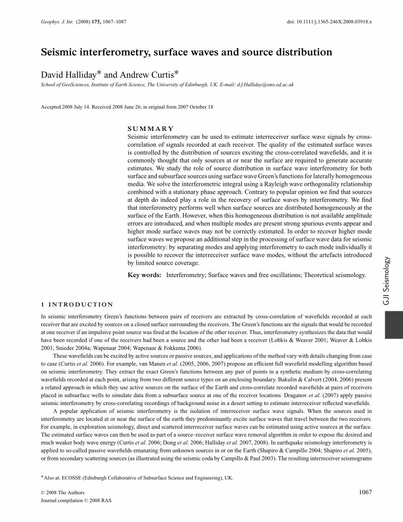
Figure 1. Geometry for eq. (1). Note that rA and rB lie beneath the free surface in this case.

2 F U L L I N T E R F E RO M E T R I C C O N S T RU C T I O N O F S U R FA C E WAV E S

We begin with the frequency domain version of the elastic interferometric formula of van Manen et al. (2006),

G∗im(rA, rB) − Gim(rA, rB)

=∫

S

{Gin(rA, r)n j cnjkl∂k G∗

ml (rB, r) − n j cnjkl∂k Gil (rA, r)G∗mn(rB, r)

}dS, (1)

where Gim(rA, rB) denotes the Green’s function representing the ith component of particle displacement at location rA due to a unidirectional,impulsive, point force in the m direction at rB (herein referred to as a monopole source), ∂k Gml (rB, r) is the partial derivative in the k directionof the Green’s function Gml (rB, r), cnjkl is the elasticity tensor, ∗ denotes complex conjugation, n j is the outward normal to the arbitrarilyshaped surface S, where S encloses the locations rA and rB (Fig. 1) and the term n j cnjkl∂k Gml (rB, r) represents the particle displacement atrB due to a deformation-rate-tensor source at r (herein referred to as a dipole source). Einstein’s summation convention applies for repeatedindices.

We assume that the portion of the earth in which we are interested is a lossless, horizontally layered medium, and that in this mediumthe wavefield is dominated by (or can be represented by) surface waves. The Green’s functions for such a medium are given by Snieder (2002,eq. 14) as

Gim(rA, rB) =∑

ν

pνi (z A, ϕ)pν∗

m (zB, ϕ)ei(kν X+ π

4 )√π

2 kν X, (2)

and (from our Appendix A)

n j cnjkl∂k Gml (rA, rB) =∑

ν

pνm(z A, ϕ)T ν∗

n (zB, ϕ)ei(kν X+ π

4 )√π

2 kν X, (3)

where z A and zB are the depths of the locations rA and rB , respectively. Here pνi is the ith component of the polarization vector

pν(z A, ϕ) =

⎡⎢⎣

r ν1 (z A) cos ϕ

r ν1 (z A) sin ϕ

ir ν2 (z A)

⎤⎥⎦ , (4)

T νn is the nth component of the traction vector

Tν(z, ϕ) = eνkln j cnjkl , (5)

or

Tν(z, ϕ) =

⎡⎢⎣

ikνr ν1 (z) cos2 ϕ ikνr ν

1 (z) cos ϕ sin ϕ −kνr ν2 (z) cos ϕ

ikνr ν1 (z) cos ϕ sin ϕ ikνr ν

1 (z) sin2 ϕ −kνr ν2 (z) sin ϕ

∂

∂z r ν1 (z) cos ϕ ∂

∂z r ν1 (z) sin ϕ ∂

∂z ir ν2 (z)

⎤⎥⎦ n j cnjkl , (6)

where eνkl = pν

l (z A, ϕ)Eνk (ϕ), kν is the wavenumber associated with the νth surface wave mode, Eν

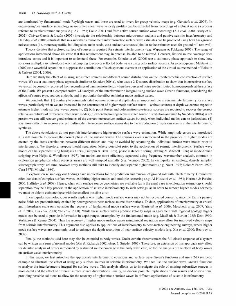
k (ϕ) is the strain operator (Appendix A), Xis the horizontal offset between the locations rA and rB , ϕ is the azimuth of the horizontal path between rA and rB (Fig. 2) and r ν

1 (z) and r ν2 (z)

are the horizontal and vertical Rayleigh wave eigenfunctions, respectively. To simplify the expression the modal normalization 8cνU ν I ν1 = 1

is assumed (Snieder 2002), where cν , U ν and I ν1 are the phase velocity, group velocity and kinetic energy for the current mode, respectively.

This Green’s function is for a single frequency, and in the following we assume summation over the relevant frequency range.Wapenaar & Fokkema (2006) show that when the integration surface S is a sphere with extremely large radius, and if the area around

S is homogeneous it is possible to approximate integrals such as eq. (1) to include a sum only over P- and S-wave source types. Since P-and S-wave sources can be written as a sum of monopole sources we can consider that it is reasonable to approximate eq. (1) using the

C© 2008 The Authors, GJI, 175, 1067–1087



Figure 2. A plan view showing geometric variables used to describe the surface wave Green’s function (eq. 2).

cross-correlation and summation of only monopole responses, that is,

G∗im(rA, rB) − Gim(rA, rB) ≈

∫S

Gin(rB, r)G∗mn(rA, r)dS. (7)

This allows interferometry to be applied to real situations where only monopole sources may be available. This approximation is discussedin more detail at the end of Section 2.2.

2.1 The effect of missing subsurface sources

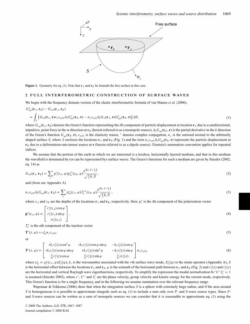
We now use a layered 2-D example to illustrate the application of exact seismic interferometry (eq. 1) before illustrating the effect of removingthe subsurface part of the boundary of sources S. Fig. 3 illustrates a layered 2-D model that generates significant higher mode surface waves(adapted from the shear wave velocity profile of Gabriels et al. 1987). We solve the eigenvalue problem for Rayleigh waves in a horizontallylayered medium to calculate displacement eigenvectors [r ν

1 (z) and r ν2 (z)] and their derivates for each of the first six modes (Lai & Rix 1998;

Aki & Richards 2002). While both the length-scale of this model and the frequencies considered are more relevant to exploration seismology,the same theory can be applied to larger scale, earthquake seismology problems. One benefit of using an example like this to illustrate our

Figure 3. (a) Geometry used in Figs 4–6. Thick dashed lines indicate the location of the integration surface, black triangles indicate the location of the receiverline, and horizontal lines indicate the free surface (top) and each successive interface below that. (b) Layer parameters.

C© 2008 The Authors, GJI, 175, 1067–1087



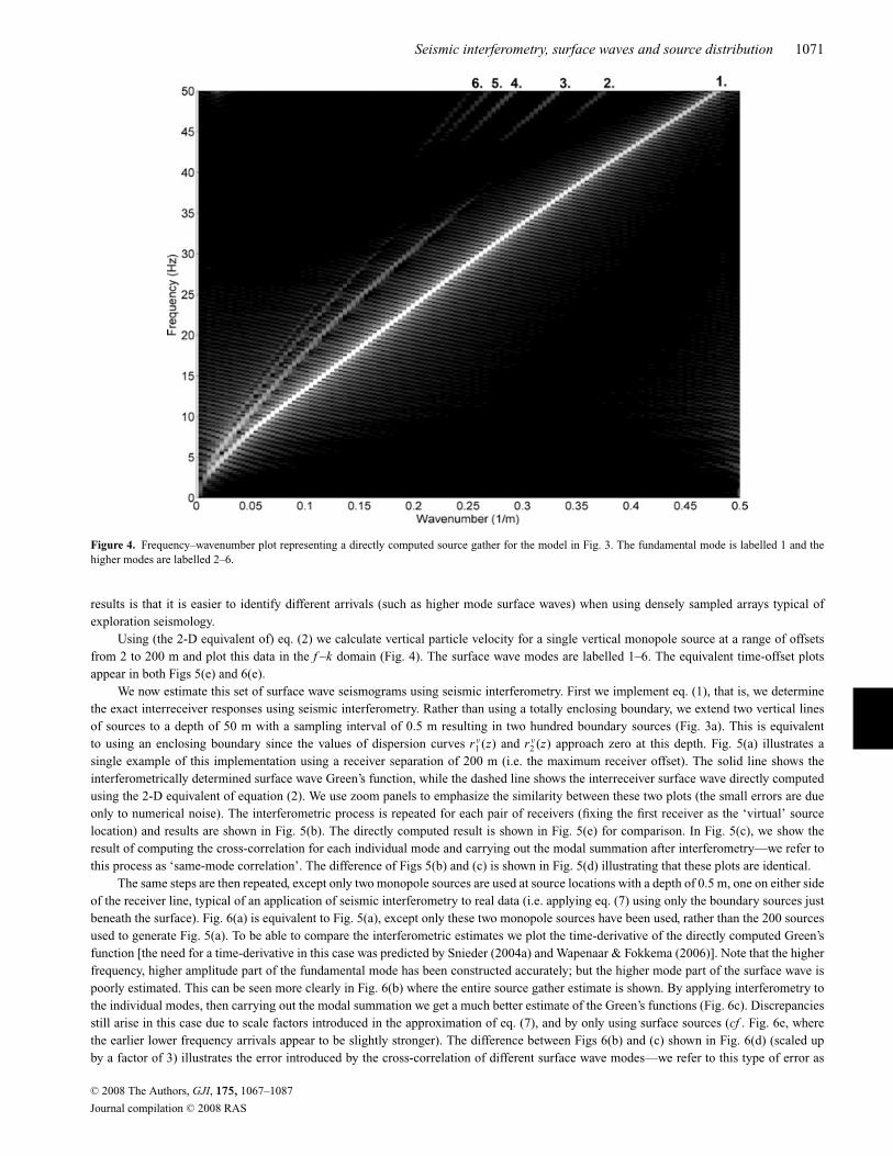
Figure 4. Frequency–wavenumber plot representing a directly computed source gather for the model in Fig. 3. The fundamental mode is labelled 1 and thehigher modes are labelled 2–6.

results is that it is easier to identify different arrivals (such as higher mode surface waves) when using densely sampled arrays typical ofexploration seismology.

Using (the 2-D equivalent of) eq. (2) we calculate vertical particle velocity for a single vertical monopole source at a range of offsetsfrom 2 to 200 m and plot this data in the f –k domain (Fig. 4). The surface wave modes are labelled 1–6. The equivalent time-offset plotsappear in both Figs 5(e) and 6(e).

We now estimate this set of surface wave seismograms using seismic interferometry. First we implement eq. (1), that is, we determinethe exact interreceiver responses using seismic interferometry. Rather than using a totally enclosing boundary, we extend two vertical linesof sources to a depth of 50 m with a sampling interval of 0.5 m resulting in two hundred boundary sources (Fig. 3a). This is equivalentto using an enclosing boundary since the values of dispersion curves r ν

1 (z) and r ν2 (z) approach zero at this depth. Fig. 5(a) illustrates a

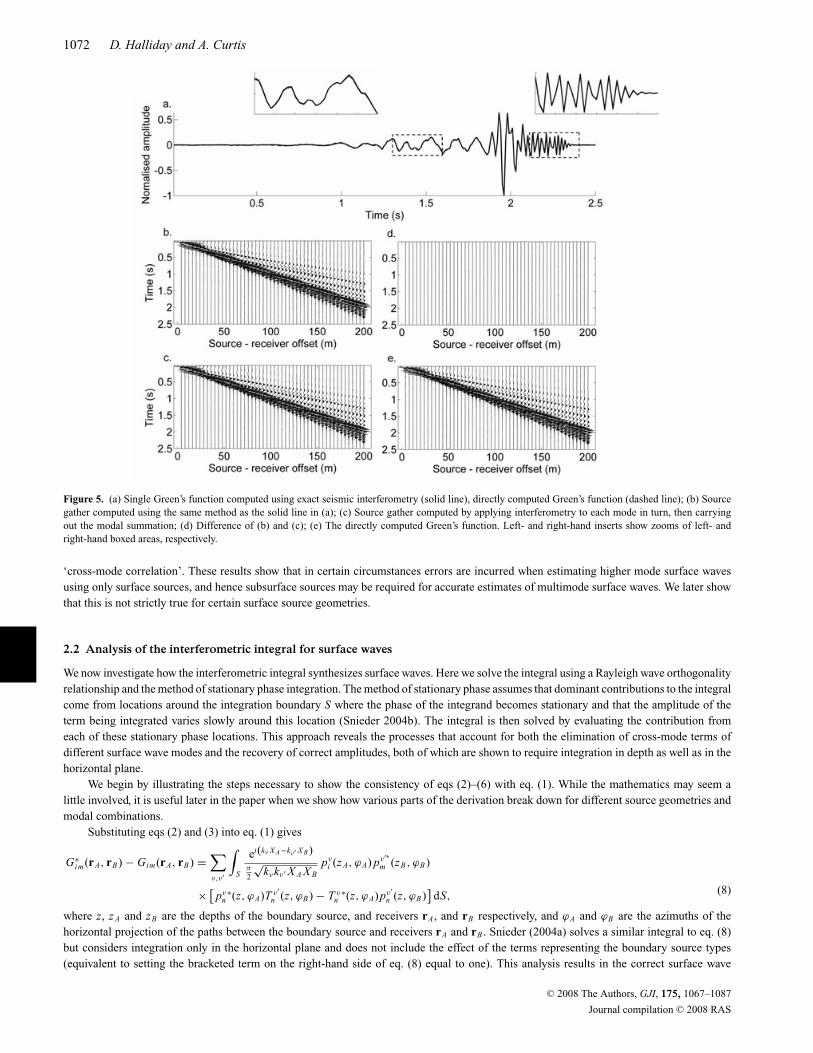
single example of this implementation using a receiver separation of 200 m (i.e. the maximum receiver offset). The solid line shows theinterferometrically determined surface wave Green’s function, while the dashed line shows the interreceiver surface wave directly computedusing the 2-D equivalent of equation (2). We use zoom panels to emphasize the similarity between these two plots (the small errors are dueonly to numerical noise). The interferometric process is repeated for each pair of receivers (fixing the first receiver as the ‘virtual’ sourcelocation) and results are shown in Fig. 5(b). The directly computed result is shown in Fig. 5(e) for comparison. In Fig. 5(c), we show theresult of computing the cross-correlation for each individual mode and carrying out the modal summation after interferometry—we refer tothis process as ‘same-mode correlation’. The difference of Figs 5(b) and (c) is shown in Fig. 5(d) illustrating that these plots are identical.

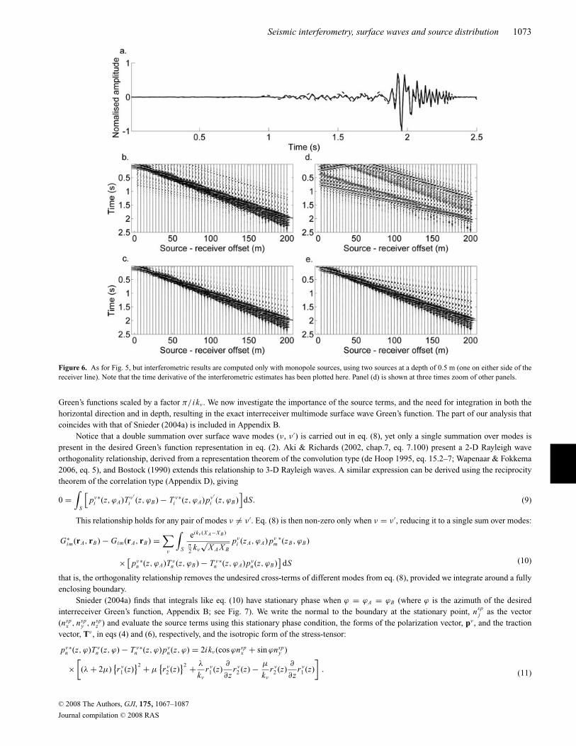
The same steps are then repeated, except only two monopole sources are used at source locations with a depth of 0.5 m, one on either sideof the receiver line, typical of an application of seismic interferometry to real data (i.e. applying eq. (7) using only the boundary sources justbeneath the surface). Fig. 6(a) is equivalent to Fig. 5(a), except only these two monopole sources have been used, rather than the 200 sourcesused to generate Fig. 5(a). To be able to compare the interferometric estimates we plot the time-derivative of the directly computed Green’sfunction [the need for a time-derivative in this case was predicted by Snieder (2004a) and Wapenaar & Fokkema (2006)]. Note that the higherfrequency, higher amplitude part of the fundamental mode has been constructed accurately; but the higher mode part of the surface wave ispoorly estimated. This can be seen more clearly in Fig. 6(b) where the entire source gather estimate is shown. By applying interferometry tothe individual modes, then carrying out the modal summation we get a much better estimate of the Green’s functions (Fig. 6c). Discrepanciesstill arise in this case due to scale factors introduced in the approximation of eq. (7), and by only using surface sources (cf . Fig. 6e, wherethe earlier lower frequency arrivals appear to be slightly stronger). The difference between Figs 6(b) and (c) shown in Fig. 6(d) (scaled upby a factor of 3) illustrates the error introduced by the cross-correlation of different surface wave modes—we refer to this type of error as

C© 2008 The Authors, GJI, 175, 1067–1087



Figure 5. (a) Single Green’s function computed using exact seismic interferometry (solid line), directly computed Green’s function (dashed line); (b) Sourcegather computed using the same method as the solid line in (a); (c) Source gather computed by applying interferometry to each mode in turn, then carryingout the modal summation; (d) Difference of (b) and (c); (e) The directly computed Green’s function. Left- and right-hand inserts show zooms of left- andright-hand boxed areas, respectively.

‘cross-mode correlation’. These results show that in certain circumstances errors are incurred when estimating higher mode surface wavesusing only surface sources, and hence subsurface sources may be required for accurate estimates of multimode surface waves. We later showthat this is not strictly true for certain surface source geometries.

2.2 Analysis of the interferometric integral for surface waves

We now investigate how the interferometric integral synthesizes surface waves. Here we solve the integral using a Rayleigh wave orthogonalityrelationship and the method of stationary phase integration. The method of stationary phase assumes that dominant contributions to the integralcome from locations around the integration boundary S where the phase of the integrand becomes stationary and that the amplitude of theterm being integrated varies slowly around this location (Snieder 2004b). The integral is then solved by evaluating the contribution fromeach of these stationary phase locations. This approach reveals the processes that account for both the elimination of cross-mode terms ofdifferent surface wave modes and the recovery of correct amplitudes, both of which are shown to require integration in depth as well as in thehorizontal plane.

We begin by illustrating the steps necessary to show the consistency of eqs (2)–(6) with eq. (1). While the mathematics may seem alittle involved, it is useful later in the paper when we show how various parts of the derivation break down for different source geometries andmodal combinations.

Substituting eqs (2) and (3) into eq. (1) gives

G∗im(rA, rB) − Gim(rA, rB) =

∑ν,ν′

∫S

ei(kν X A−kν′ X B)

π

2

√kνkν′ X A X B

pνi (z A, ϕA) pν′∗

m (zB, ϕB)

× [pν

n∗(z, ϕA)T ν′

n (z, ϕB) − T νn

∗(z, ϕA)pν′n (z, ϕB)

]dS,

(8)

where z, z A and zB are the depths of the boundary source, and receivers rA, and rB respectively, and ϕA and ϕB are the azimuths of thehorizontal projection of the paths between the boundary source and receivers rA and rB . Snieder (2004a) solves a similar integral to eq. (8)but considers integration only in the horizontal plane and does not include the effect of the terms representing the boundary source types(equivalent to setting the bracketed term on the right-hand side of eq. (8) equal to one). This analysis results in the correct surface wave

C© 2008 The Authors, GJI, 175, 1067–1087



Figure 6. As for Fig. 5, but interferometric results are computed only with monopole sources, using two sources at a depth of 0.5 m (one on either side of thereceiver line). Note that the time derivative of the interferometric estimates has been plotted here. Panel (d) is shown at three times zoom of other panels.

Green’s functions scaled by a factor π/ ikν . We now investigate the importance of the source terms, and the need for integration in both thehorizontal direction and in depth, resulting in the exact interreceiver multimode surface wave Green’s function. The part of our analysis thatcoincides with that of Snieder (2004a) is included in Appendix B.

Notice that a double summation over surface wave modes (ν, ν ′) is carried out in eq. (8), yet only a single summation over modes ispresent in the desired Green’s function representation in eq. (2). Aki & Richards (2002, chap.7, eq. 7.100) present a 2-D Rayleigh waveorthogonality relationship, derived from a representation theorem of the convolution type (de Hoop 1995, eq. 15.2–7; Wapenaar & Fokkema2006, eq. 5), and Bostock (1990) extends this relationship to 3-D Rayleigh waves. A similar expression can be derived using the reciprocitytheorem of the correlation type (Appendix D), giving

0 =∫

S

[pν

i∗(z, ϕA)T ν′

i (z, ϕB) − T νi

∗(z, ϕA)pν′i (z, ϕB)

]dS. (9)

This relationship holds for any pair of modes ν �= ν ′. Eq. (8) is then non-zero only when ν = ν ′, reducing it to a single sum over modes:


∑ν

∫S

eikν (X A−X B )

π

2 kν

√X A X B

pνi (z A, ϕA) pν

m∗(zB, ϕB)

× [pν

n∗(z, ϕA)T ν

n (z, ϕB) − T νn

∗(z, ϕA)pνn (z, ϕB)

]dS (10)

that is, the orthogonality relationship removes the undesired cross-terms of different modes from eq. (8), provided we integrate around a fullyenclosing boundary.

Snieder (2004a) finds that integrals like eq. (10) have stationary phase when ϕ = ϕA = ϕB (where ϕ is the azimuth of the desiredinterreceiver Green’s function, Appendix B; see Fig. 7). We write the normal to the boundary at the stationary point, nsp

j as the vector(nsp

x , nspy , nsp

z ) and evaluate the source terms using this stationary phase condition, the forms of the polarization vector, pν , and the tractionvector, Tν , in eqs (4) and (6), respectively, and the isotropic form of the stress-tensor:

pνn∗(z, ϕ)T ν

n (z, ϕ) − T νn

∗(z, ϕ)pνn (z, ϕ) = 2ikν(cos ϕnsp

x + sin ϕnspy )

×[

(λ + 2μ){r ν

1 (z)}2 + μ

{r ν

2 (z)}2 + λ

kν

r ν1 (z)

∂

∂zr ν

2 (z) − μ

kν

r ν2 (z)

∂

∂zr ν

1 (z)

]. (11)

C© 2008 The Authors, GJI, 175, 1067–1087



Figure 7. Geometric configuration for a stationary point for the direct surface wave.

Using the energy integrals (Aki & Richards 2002, chap. 7, eq. 7.74)

I ν2 = 1

2

∫ ∞

0

[(λ + 2μ)

{r ν

1 (z)}2 + μ

{r ν

2 (z)}2]

dz, (12)

and

I ν3 =

∫ ∞

0

[λr ν

1 (z)∂r ν

2 (z)

∂z− μr ν

2 (z)∂r ν

1 (z)

∂z

]dz, (13)

allows the integration of eq. (11) over depth to be written as∫ ∞

0

[pν

n∗(z, ϕ)T ν

n (z, ϕ) − T νn

∗(z, ϕ)pνn (z, ϕ)

]dz = 2ikν(cos ϕnsp

x + sin ϕnspy )

[2I ν

2 + I ν3

kν

]. (14)

Thus we have solved the part of the integral dependent on depth. Using eq. (7.76) from Aki & Richards (2002), I ν2 + I ν

3 /2kν = cνU ν I ν1 ,

and recalling from the definition after eq. (6) that 8cνU ν I ν1 = 1, then

G∗im(rA, rB) − Gim(rA, rB) ≈

∑ν

ikν

π

∫S

eikν (X A−X B )

kν

√X A X B

pνi (z A, ϕ) pν

m∗(zB, ϕ)dS

× (cos ϕnsp

x + sin ϕnspy

). (15)

In Appendix B, we show that this integral can be solved following the stationary phase argument of Snieder (2004a), resulting in

G∗im(rA, rB) − Gim(rA, rB) ≈ −η

∑ν

pνi (z A, ϕ) pν

m∗(zB, ϕ)

eiη(kν X+ π4 )√

π

2 kν X, (16)

where X is the horizontal offset between rA and rB . There are two types of stationary phase location, one where X A < X B and one whereX A > X B , these two cases are denoted by η = −1 and η = 1, respectively. This result is virtually identical to eq. (2), the only differencebeing that in eq. (16) both causal (forward time) and acausal (reverse time) Green’s functions exist. Note that by considering source terms andintegration in depth we have not only correctly accounted for the higher mode surface waves, but we have also accounted for the factor π/ ikν

introduced in the analysis of Snieder (2004a). This result is illustrated in Fig. 5, where we have plotted the causal part of the interferometricallydetermined Green’s functions.

In eq. (7), we approximated the interferometric integral to be a sum over only point-force sources. In Appendix C, we investigate theeffect of this approximation and using the far-field condition we derive a scale factor allowing us to quantify the effect of using only monopolesources, as is common in applications of interferometry to real data. We find that eq. (7) can be rewritten as

G∗im(rA, rB) − Gim(rA, rB) ≈ ikν

∫S

Mν(ω)Gin(rB, r)G∗mn(rA, r)dS, (17)

where Mν(ω) is a scale factor accounting for the changes introduced by using only monopole sources, given by

Mν(ω) = 2n j cνU νρ. (18)

We can expect results using only monopole sources to vary with frequency (ω), surface wave mode (ν), and the near-surface density,ρ. The term ikν (= iω/cν) can partly be accounted for with a time derivative (in the frequency domain a time derivative is equivalent tomultiplication by iω). This is the only term that affects the phase of the Green’s function (for a single frequency); hence, without accountingfor the rest of the scale factor we can still expect the estimated surface wave to have the correct phase. Note that the presence of higher modescomplicates the application of the term iω/cν , as it varies for each mode. Of course, methods exist to estimate local material properties (e.g.Aki 1957; Curtis & Robertsson 2002; van Vossen et al. 2005), and it is possible to identify and separate different surface wave modes using

C© 2008 The Authors, GJI, 175, 1067–1087



array based frequency–wavenumber methods, or single-station methods (e.g. van Heijst & Woodhouse 1997). Hence, if required, these scalefactors could be estimated and used explicitly.

In Appendix C, we note that a similar approach to the above can be used to solve the single source-type interferometric integral (eq. 17).In this case, due to complications with scale factors we have neglected the effect of higher mode surface waves. However, in Appendix D wealso derive a Rayleigh wave orthogonality relationship for the single source case. Hence, apart from varying scale factors, we expect sourcesat depth to play a similar role in this case.

3 I N T E R F E RO M E T RY W I T H O N LY S U R FA C E S O U RC E S

In practise the most likely case is that sources will only be available at (or near) the surface of the earth as this is the usual case in active sourceseismology, and also in passive interferometry where passive wavefields are believed to be excited by predominantly near-surface sources(Shapiro & Campillo 2004; Shapiro et al. 2005). Here we illustrate the effect of different surface source distributions on the estimation ofinterreceiver surface waves, for both single and multimode cases.

3.1 Surface source distribution—single mode surface waves

Snieder (2004a) considers a homogeneous distribution of sources at the surface of the Earth and shows that the correct interreceiver surfacewave can be recovered, and we begin by illustrating this case. The scale factor in eq. (17) applies when a fully enclosing boundary of sourcesis present. Since we now only use sources at the surface, and terms such as eqs (12)–(14) which require integration in depth do not hold, thisscale factor no longer applies. Here we use a single mode, hence there are no complications due to varying scale factors for different modes.To account for the lack of sources at depth we introduce a modal and frequency dependent scale factor, Aν(ω), that may differ from Mν(ω)depending on source configurations. For this homogeneous distribution we replace the integration surface S by integration over the x- andy-coordinates,

Gestim(rA, rB) ≈ ikν Aν(ω)

∫ y2

y1

∫ x2

x1

Gin(rB, r)G∗mn(rA, r) dx dy. (19)

Here we define the estimated Green’s function resulting from the chosen source geometry as Gestim (rA, rB). Using the simple case of a

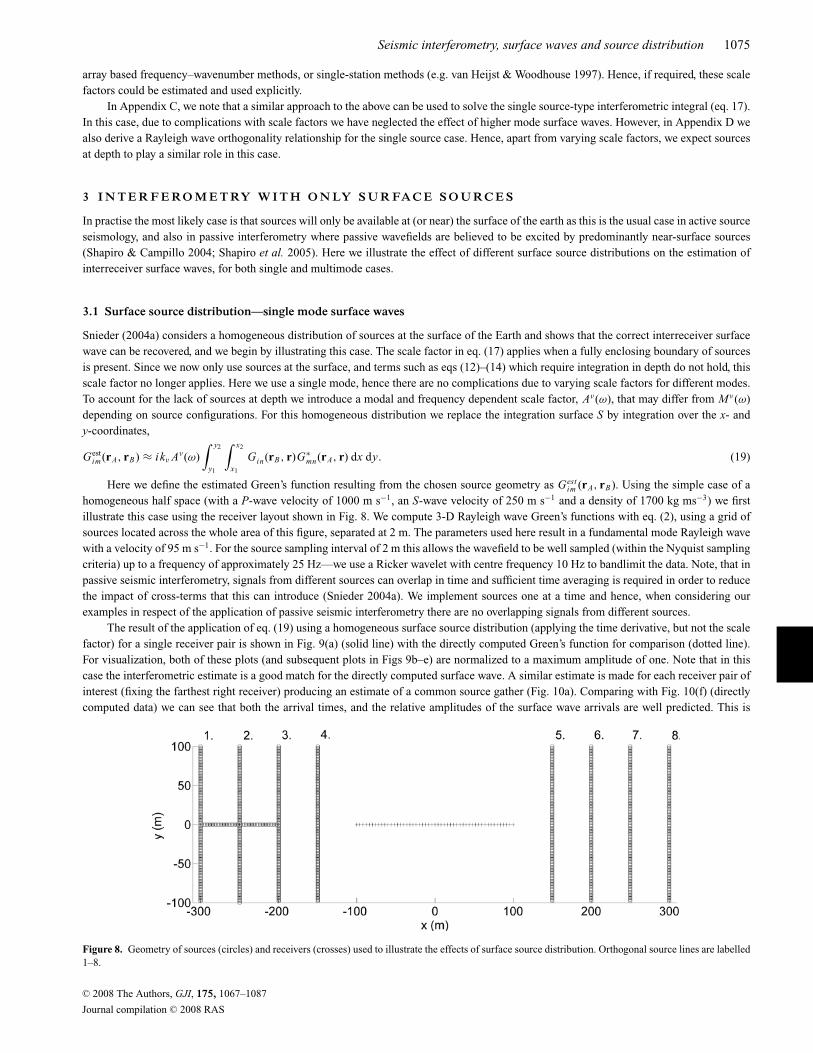
homogeneous half space (with a P-wave velocity of 1000 m s−1, an S-wave velocity of 250 m s−1 and a density of 1700 kg ms−3) we firstillustrate this case using the receiver layout shown in Fig. 8. We compute 3-D Rayleigh wave Green’s functions with eq. (2), using a grid ofsources located across the whole area of this figure, separated at 2 m. The parameters used here result in a fundamental mode Rayleigh wavewith a velocity of 95 m s−1. For the source sampling interval of 2 m this allows the wavefield to be well sampled (within the Nyquist samplingcriteria) up to a frequency of approximately 25 Hz—we use a Ricker wavelet with centre frequency 10 Hz to bandlimit the data. Note, that inpassive seismic interferometry, signals from different sources can overlap in time and sufficient time averaging is required in order to reducethe impact of cross-terms that this can introduce (Snieder 2004a). We implement sources one at a time and hence, when considering ourexamples in respect of the application of passive seismic interferometry there are no overlapping signals from different sources.

The result of the application of eq. (19) using a homogeneous surface source distribution (applying the time derivative, but not the scalefactor) for a single receiver pair is shown in Fig. 9(a) (solid line) with the directly computed Green’s function for comparison (dotted line).For visualization, both of these plots (and subsequent plots in Figs 9b–e) are normalized to a maximum amplitude of one. Note that in thiscase the interferometric estimate is a good match for the directly computed surface wave. A similar estimate is made for each receiver pair ofinterest (fixing the farthest right receiver) producing an estimate of a common source gather (Fig. 10a). Comparing with Fig. 10(f) (directlycomputed data) we can see that both the arrival times, and the relative amplitudes of the surface wave arrivals are well predicted. This is

Figure 8. Geometry of sources (circles) and receivers (crosses) used to illustrate the effects of surface source distribution. Orthogonal source lines are labelled1–8.

C© 2008 The Authors, GJI, 175, 1067–1087



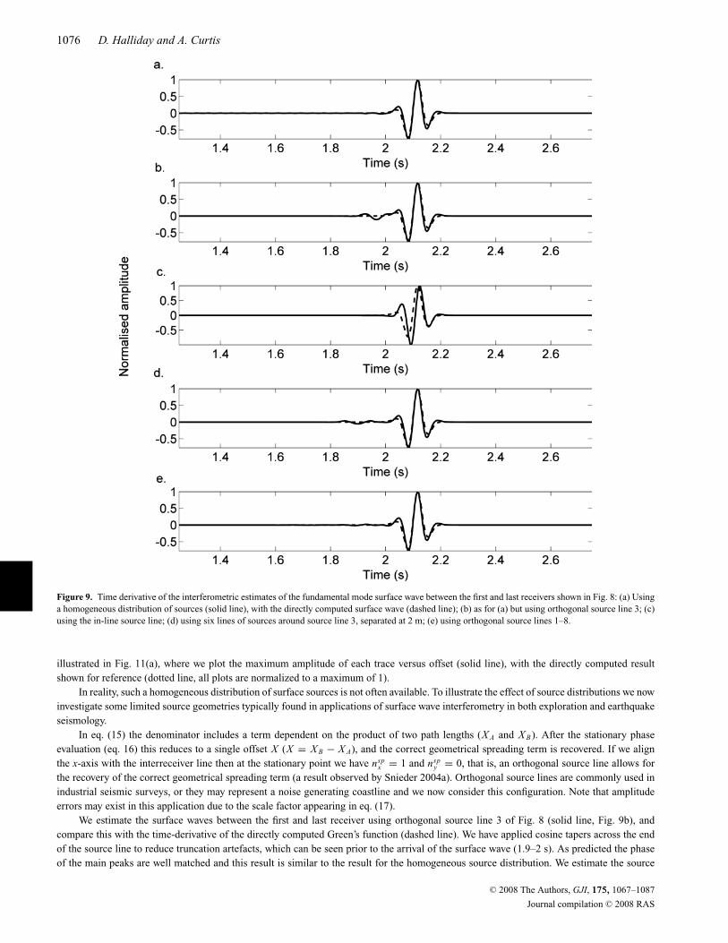
Figure 9. Time derivative of the interferometric estimates of the fundamental mode surface wave between the first and last receivers shown in Fig. 8: (a) Usinga homogeneous distribution of sources (solid line), with the directly computed surface wave (dashed line); (b) as for (a) but using orthogonal source line 3; (c)using the in-line source line; (d) using six lines of sources around source line 3, separated at 2 m; (e) using orthogonal source lines 1–8.

illustrated in Fig. 11(a), where we plot the maximum amplitude of each trace versus offset (solid line), with the directly computed resultshown for reference (dotted line, all plots are normalized to a maximum of 1).

In reality, such a homogeneous distribution of surface sources is not often available. To illustrate the effect of source distributions we nowinvestigate some limited source geometries typically found in applications of surface wave interferometry in both exploration and earthquakeseismology.

In eq. (15) the denominator includes a term dependent on the product of two path lengths (X A and X B). After the stationary phaseevaluation (eq. 16) this reduces to a single offset X (X = X B − X A), and the correct geometrical spreading term is recovered. If we alignthe x-axis with the interreceiver line then at the stationary point we have nsp

x = 1 and nspy = 0, that is, an orthogonal source line allows for

the recovery of the correct geometrical spreading term (a result observed by Snieder 2004a). Orthogonal source lines are commonly used inindustrial seismic surveys, or they may represent a noise generating coastline and we now consider this configuration. Note that amplitudeerrors may exist in this application due to the scale factor appearing in eq. (17).

We estimate the surface waves between the first and last receiver using orthogonal source line 3 of Fig. 8 (solid line, Fig. 9b), andcompare this with the time-derivative of the directly computed Green’s function (dashed line). We have applied cosine tapers across the endof the source line to reduce truncation artefacts, which can be seen prior to the arrival of the surface wave (1.9–2 s). As predicted the phaseof the main peaks are well matched and this result is similar to the result for the homogeneous source distribution. We estimate the source

C© 2008 The Authors, GJI, 175, 1067–1087



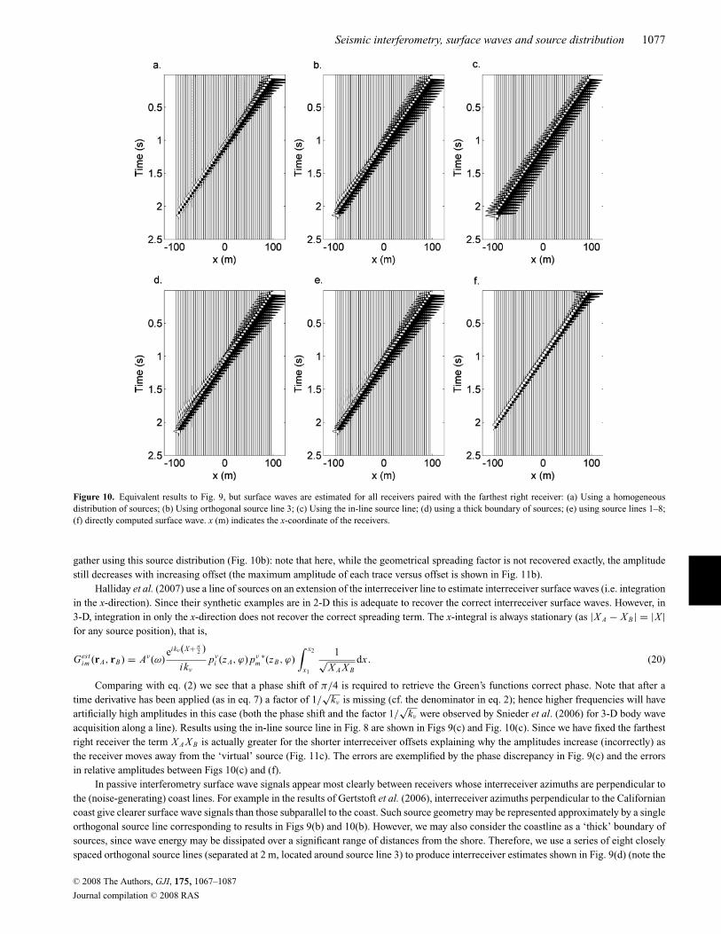
Figure 10. Equivalent results to Fig. 9, but surface waves are estimated for all receivers paired with the farthest right receiver: (a) Using a homogeneousdistribution of sources; (b) Using orthogonal source line 3; (c) Using the in-line source line; (d) using a thick boundary of sources; (e) using source lines 1–8;(f) directly computed surface wave. x (m) indicates the x-coordinate of the receivers.

gather using this source distribution (Fig. 10b): note that here, while the geometrical spreading factor is not recovered exactly, the amplitudestill decreases with increasing offset (the maximum amplitude of each trace versus offset is shown in Fig. 11b).

Halliday et al. (2007) use a line of sources on an extension of the interreceiver line to estimate interreceiver surface waves (i.e. integrationin the x-direction). Since their synthetic examples are in 2-D this is adequate to recover the correct interreceiver surface waves. However, in3-D, integration in only the x-direction does not recover the correct spreading term. The x-integral is always stationary (as |X A − X B | = |X |for any source position), that is,

Gestim (rA, rB) = Aν(ω)

eikν(X+ π2 )

ikν

pνi (z A, ϕ) pν

m∗(zB, ϕ)

∫ x2

x1

1√X A X B

dx . (20)

Comparing with eq. (2) we see that a phase shift of π/4 is required to retrieve the Green’s functions correct phase. Note that after atime derivative has been applied (as in eq. 7) a factor of 1/

√kν is missing (cf. the denominator in eq. 2); hence higher frequencies will have

artificially high amplitudes in this case (both the phase shift and the factor 1/√

kν were observed by Snieder et al. (2006) for 3-D body waveacquisition along a line). Results using the in-line source line in Fig. 8 are shown in Figs 9(c) and Fig. 10(c). Since we have fixed the farthestright receiver the term X A X B is actually greater for the shorter interreceiver offsets explaining why the amplitudes increase (incorrectly) asthe receiver moves away from the ‘virtual’ source (Fig. 11c). The errors are exemplified by the phase discrepancy in Fig. 9(c) and the errorsin relative amplitudes between Figs 10(c) and (f).

In passive interferometry surface wave signals appear most clearly between receivers whose interreceiver azimuths are perpendicular tothe (noise-generating) coast lines. For example in the results of Gertstoft et al. (2006), interreceiver azimuths perpendicular to the Californiancoast give clearer surface wave signals than those subparallel to the coast. Such source geometry may be represented approximately by a singleorthogonal source line corresponding to results in Figs 9(b) and 10(b). However, we may also consider the coastline as a ‘thick’ boundary ofsources, since wave energy may be dissipated over a significant range of distances from the shore. Therefore, we use a series of eight closelyspaced orthogonal source lines (separated at 2 m, located around source line 3) to produce interreceiver estimates shown in Fig. 9(d) (note the

C© 2008 The Authors, GJI, 175, 1067–1087



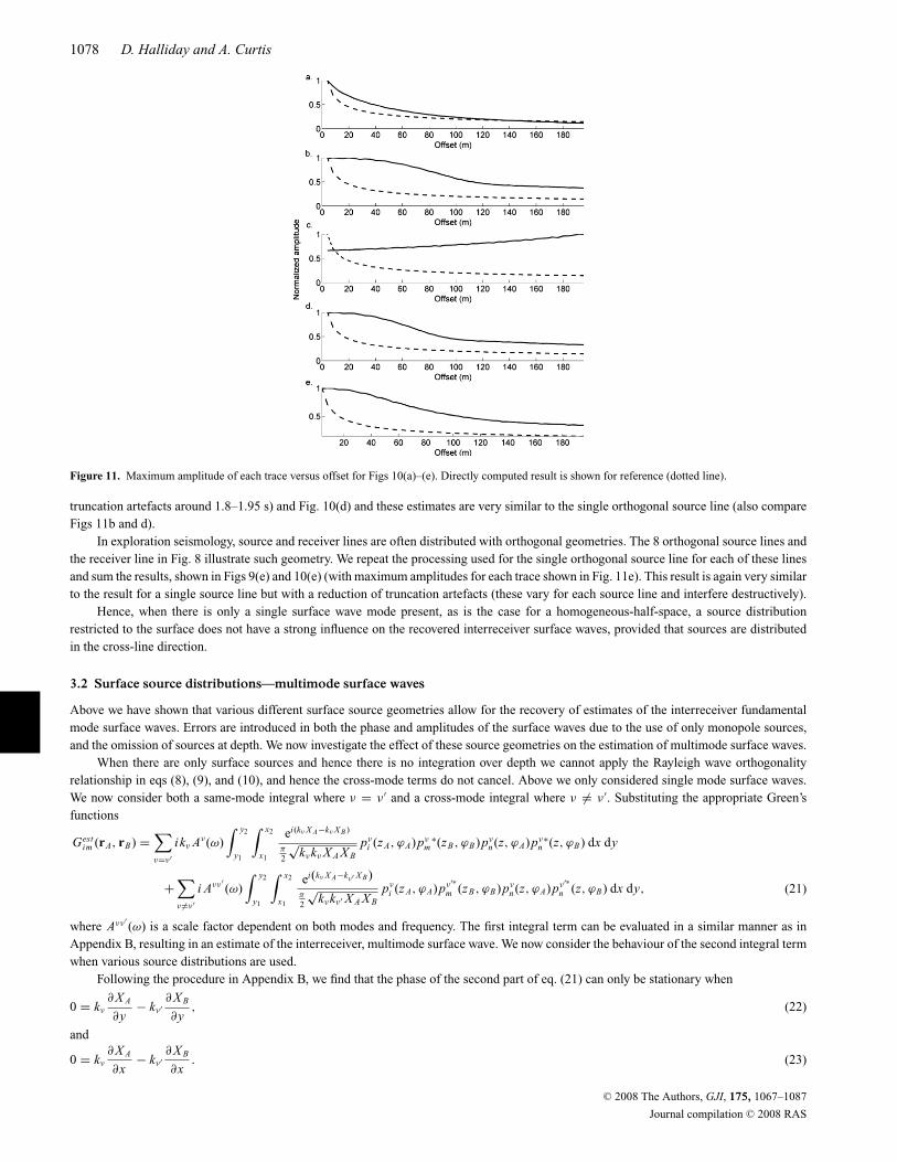
Figure 11. Maximum amplitude of each trace versus offset for Figs 10(a)–(e). Directly computed result is shown for reference (dotted line).

truncation artefacts around 1.8–1.95 s) and Fig. 10(d) and these estimates are very similar to the single orthogonal source line (also compareFigs 11b and d).

In exploration seismology, source and receiver lines are often distributed with orthogonal geometries. The 8 orthogonal source lines andthe receiver line in Fig. 8 illustrate such geometry. We repeat the processing used for the single orthogonal source line for each of these linesand sum the results, shown in Figs 9(e) and 10(e) (with maximum amplitudes for each trace shown in Fig. 11e). This result is again very similarto the result for a single source line but with a reduction of truncation artefacts (these vary for each source line and interfere destructively).

Hence, when there is only a single surface wave mode present, as is the case for a homogeneous-half-space, a source distributionrestricted to the surface does not have a strong influence on the recovered interreceiver surface waves, provided that sources are distributedin the cross-line direction.

3.2 Surface source distributions—multimode surface waves

Above we have shown that various different surface source geometries allow for the recovery of estimates of the interreceiver fundamentalmode surface waves. Errors are introduced in both the phase and amplitudes of the surface waves due to the use of only monopole sources,and the omission of sources at depth. We now investigate the effect of these source geometries on the estimation of multimode surface waves.

When there are only surface sources and hence there is no integration over depth we cannot apply the Rayleigh wave orthogonalityrelationship in eqs (8), (9), and (10), and hence the cross-mode terms do not cancel. Above we only considered single mode surface waves.We now consider both a same-mode integral where ν = ν ′ and a cross-mode integral where ν �= ν ′. Substituting the appropriate Green’sfunctions

Gestim (rA, rB) =

∑ν=ν′

ikν Aν(ω)∫ y2

y1

∫ x2

x1

ei(kν X A−kν X B )

π

2

√kνkν X A X B

pνi (z A, ϕA)pν

m∗(zB, ϕB)pν

n (z, ϕA)pνn∗(z, ϕB) dx dy

+∑ν �=ν′

i Aνν′(ω)

∫ y2

y1

∫ x2

x1

ei(kν X A−kν′ X B)

π

2

√kνkν′ X A X B

pνi (z A, ϕA)pν′∗

m (zB, ϕB)pνn (z, ϕA)pν′∗

n (z, ϕB) dx dy, (21)

where Aνν′(ω) is a scale factor dependent on both modes and frequency. The first integral term can be evaluated in a similar manner as in

Appendix B, resulting in an estimate of the interreceiver, multimode surface wave. We now consider the behaviour of the second integral termwhen various source distributions are used.

Following the procedure in Appendix B, we find that the phase of the second part of eq. (21) can only be stationary when

0 = kν

∂ X A

∂y− kν′

∂ X B

∂y, (22)

and

0 = kν

∂ X A

∂x− kν′

∂ X B

∂x. (23)

C© 2008 The Authors, GJI, 175, 1067–1087



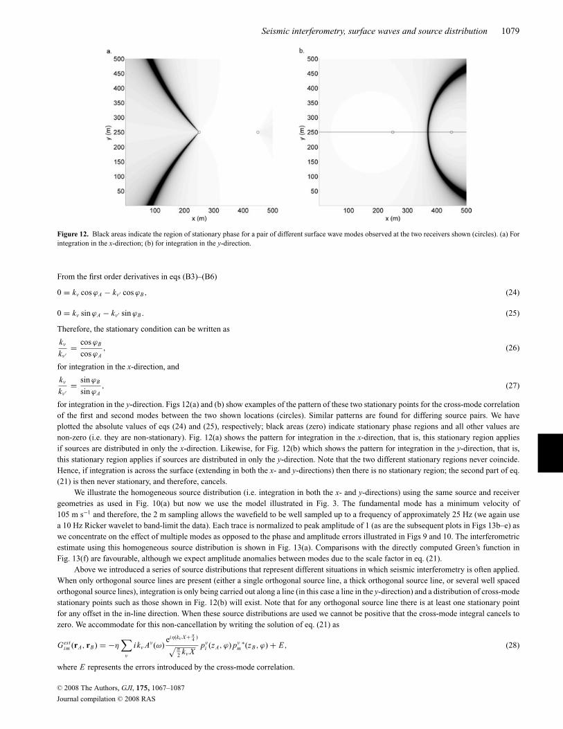
Figure 12. Black areas indicate the region of stationary phase for a pair of different surface wave modes observed at the two receivers shown (circles). (a) Forintegration in the x-direction; (b) for integration in the y-direction.

From the first order derivatives in eqs (B3)–(B6)

0 = kν cos ϕA − kν′ cos ϕB, (24)

0 = kν sin ϕA − kν′ sin ϕB . (25)

Therefore, the stationary condition can be written as

kν

kν′= cos ϕB

cos ϕA, (26)

for integration in the x-direction, and

kν

kν′= sin ϕB

sin ϕA, (27)

for integration in the y-direction. Figs 12(a) and (b) show examples of the pattern of these two stationary points for the cross-mode correlationof the first and second modes between the two shown locations (circles). Similar patterns are found for differing source pairs. We haveplotted the absolute values of eqs (24) and (25), respectively; black areas (zero) indicate stationary phase regions and all other values arenon-zero (i.e. they are non-stationary). Fig. 12(a) shows the pattern for integration in the x-direction, that is, this stationary region appliesif sources are distributed in only the x-direction. Likewise, for Fig. 12(b) which shows the pattern for integration in the y-direction, that is,this stationary region applies if sources are distributed in only the y-direction. Note that the two different stationary regions never coincide.Hence, if integration is across the surface (extending in both the x- and y-directions) then there is no stationary region; the second part of eq.(21) is then never stationary, and therefore, cancels.

We illustrate the homogeneous source distribution (i.e. integration in both the x- and y-directions) using the same source and receivergeometries as used in Fig. 10(a) but now we use the model illustrated in Fig. 3. The fundamental mode has a minimum velocity of105 m s−1 and therefore, the 2 m sampling allows the wavefield to be well sampled up to a frequency of approximately 25 Hz (we again usea 10 Hz Ricker wavelet to band-limit the data). Each trace is normalized to peak amplitude of 1 (as are the subsequent plots in Figs 13b–e) aswe concentrate on the effect of multiple modes as opposed to the phase and amplitude errors illustrated in Figs 9 and 10. The interferometricestimate using this homogeneous source distribution is shown in Fig. 13(a). Comparisons with the directly computed Green’s function inFig. 13(f) are favourable, although we expect amplitude anomalies between modes due to the scale factor in eq. (21).

Above we introduced a series of source distributions that represent different situations in which seismic interferometry is often applied.When only orthogonal source lines are present (either a single orthogonal source line, a thick orthogonal source line, or several well spacedorthogonal source lines), integration is only being carried out along a line (in this case a line in the y-direction) and a distribution of cross-modestationary points such as those shown in Fig. 12(b) will exist. Note that for any orthogonal source line there is at least one stationary pointfor any offset in the in-line direction. When these source distributions are used we cannot be positive that the cross-mode integral cancels tozero. We accommodate for this non-cancellation by writing the solution of eq. (21) as

Gestim (rA, rB) = −η

∑ν

ikν Aν(ω)eiη(kν X+ π

4 )√π

2 kν Xpν

i (z A, ϕ) pνm

∗(zB, ϕ) + E, (28)

where E represents the errors introduced by the cross-mode correlation.

C© 2008 The Authors, GJI, 175, 1067–1087



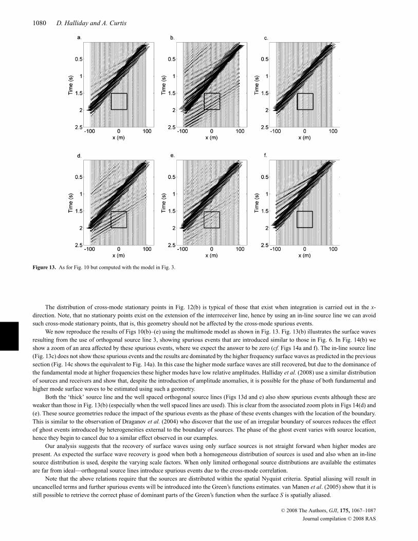
Figure 13. As for Fig. 10 but computed with the model in Fig. 3.

The distribution of cross-mode stationary points in Fig. 12(b) is typical of those that exist when integration is carried out in the x-direction. Note, that no stationary points exist on the extension of the interreceiver line, hence by using an in-line source line we can avoidsuch cross-mode stationary points, that is, this geometry should not be affected by the cross-mode spurious events.

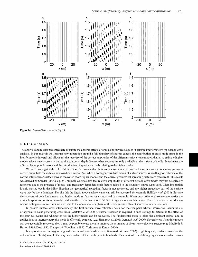
We now reproduce the results of Figs 10(b)–(e) using the multimode model as shown in Fig. 13. Fig. 13(b) illustrates the surface wavesresulting from the use of orthogonal source line 3, showing spurious events that are introduced similar to those in Fig. 6. In Fig. 14(b) weshow a zoom of an area affected by these spurious events, where we expect the answer to be zero (cf. Figs 14a and f). The in-line source line(Fig. 13c) does not show these spurious events and the results are dominated by the higher frequency surface waves as predicted in the previoussection (Fig. 14c shows the equivalent to Fig. 14a). In this case the higher mode surface waves are still recovered, but due to the dominance ofthe fundamental mode at higher frequencies these higher modes have low relative amplitudes. Halliday et al. (2008) use a similar distributionof sources and receivers and show that, despite the introduction of amplitude anomalies, it is possible for the phase of both fundamental andhigher mode surface waves to be estimated using such a geometry.

Both the ‘thick’ source line and the well spaced orthogonal source lines (Figs 13d and e) also show spurious events although these areweaker than those in Fig. 13(b) (especially when the well spaced lines are used). This is clear from the associated zoom plots in Figs 14(d) and(e). These source geometries reduce the impact of the spurious events as the phase of these events changes with the location of the boundary.This is similar to the observation of Draganov et al. (2004) who discover that the use of an irregular boundary of sources reduces the effectof ghost events introduced by heterogeneities external to the boundary of sources. The phase of the ghost event varies with source location,hence they begin to cancel due to a similar effect observed in our examples.

Our analysis suggests that the recovery of surface waves using only surface sources is not straight forward when higher modes arepresent. As expected the surface wave recovery is good when both a homogeneous distribution of sources is used and also when an in-linesource distribution is used, despite the varying scale factors. When only limited orthogonal source distributions are available the estimatesare far from ideal—orthogonal source lines introduce spurious events due to the cross-mode correlation.

Note that the above relations require that the sources are distributed within the spatial Nyquist criteria. Spatial aliasing will result inuncancelled terms and further spurious events will be introduced into the Green’s functions estimates. van Manen et al. (2005) show that it isstill possible to retrieve the correct phase of dominant parts of the Green’s function when the surface S is spatially aliased.

C© 2008 The Authors, GJI, 175, 1067–1087



Figure 14. Zoom of boxed areas in Fig. 13.

4 D I S C U S S I O N

The analysis and results presented here illustrate the adverse effects of only using surface sources in seismic interferometry for surface waveanalysis. In our analysis we illustrate how integration around a full boundary of sources cancels the contribution of cross-mode terms in theinterferometric integral and allows for the recovery of the correct amplitudes of the different surface wave modes, that is, to estimate highermode surface waves correctly we require sources at depth. Hence, when sources are only available at the surface of the Earth estimates areaffected by amplitude errors and the introduction of spurious arrivals relating to the higher modes.

We have investigated the role of different surface source distributions in seismic interferometry for surface waves. When integration iscarried out in both the in-line and cross-line direction (i.e. when a homogeneous distribution of surface sources is used) a good estimate of thecorrect interreceiver surface wave is recovered (both higher modes, and the correct geometrical spreading factors are recovered). This resultwas derived by Snieder (2004a, eq. 24), but here we also show that relative amplitudes of different surface wave modes may not be correctlyrecovered due to the presence of modal- and frequency-dependent scale factors, related to the boundary source types used. When integrationis only carried out in the inline direction the geometrical spreading factor is not recovered, and the higher frequency part of the surfacewave may be more dominant. Despite this the higher mode surface waves can still be recovered, for example Halliday et al. (2008) illustratethe recovery of both fundamental and higher mode surface waves using a real data example. When only orthogonal source geometries areavailable spurious events are introduced due to the cross-correlation of different higher mode surface waves. These errors are reduced whenseveral orthogonal source lines are used due to the non-stationary phase of the error across different source boundary locations.

In passive surface wave interferometry, the best surface wave estimates occur for receiver pairs whose interreceiver azimuths areorthogonal to noise generating coast lines (Gertstoft et al. 2006). Further research is required in such settings to determine the effect ofthe spurious events and whether or not the higher-modes can be recovered. The fundamental mode is often the dominant arrival, and inapplications of interferometry this mode is efficiently extracted (e.g. Shapiro et al. 2005; Gertstoft et al. 2006). Nevertheless if multiple modescan be successfully recovered then it may be possible to use these to improve the estimates of shear wave velocity structure (e.g. MacBeth &Burton 1985; Dost 1990; Trampert & Woodhouse 1995; Yoshizawa & Kennet 2004).

In exploration seismology orthogonal source- and receiver-lines are often used (Vermeer 2002). High frequency surface waves (on theorder of tens of hertz) sample the very near-surface of the Earth (tens to hundreds of metres), often exhibiting higher mode surface waves

C© 2008 The Authors, GJI, 175, 1067–1087



(e.g. Al-Husseini et al. 1981; Halliday et al. 2008). Hence the errors illustrated above may have a more significant impact in exploration thanin earthquake seismology. This also applies to engineering settings where high frequency, higher mode surface waves are used to invert forshear wave velocity profiles, providing extra information that can not be extracted from the fundamental mode alone (e.g. Xia et al. 2000;Beaty et al. 2002).

Due to these cross-mode errors pre-processing may be required to recover higher mode surface waves successfully with only surfacesources. Such pre-processing may be easier to apply in exploration or engineering seismology with well sampled receiver arrays allowing forseparation of modes, for example, in the frequency–wavenumber domain (e.g. Vermeer 2002). In earthquake seismology, mode separationcan be attempted using bandpass filters (e.g. Crampin & Bath 1965), phase matched filtering (e.g. Hwang & Mitchell 1986) but detailedanalysis and isolation of higher mode Rayleigh waves typically requires array measurements (e.g. Nolet 1975; Nolet & Panza 1976; Cara1978; Mitchel 1980), although single-station methods do exist (e.g. van Heijst & Woodhouse 1997). Densely sampled arrays are seldomavailable, and hence it may be more difficult to identify and separate all higher mode surface waves.

5 C O N C LU S I O N S

We have investigated seismic interferometry for surface waves using Green’s functions terms for surface waves in laterally homogeneousmedia. This analysis has revealed that there are two key components to the application of full and exact interferometry:

1. Integration over a fully enclosing boundary allows for the cancellation of cross-mode terms by the Rayleigh wave orthogonalityrelationship.

2. Integration in the cross-line direction allows for the retrieval of the correct spreading terms in the surface wave Green’s functions (aresult previously derived by Snieder 2004a, eq. 24).

Both of these components play an important role in recovering the correct relative amplitudes for different surface wave modes. Using only asingle source type provides similar results, with the introduction of a frequency- and modal-dependent scaling term that varies depending onsource geometries. When sources are not present in the subsurface further scaling terms may emerge, cross-mode terms may not cancel, andspurious events can be introduced when attempting to recover higher mode surface waves.

The insight provided by this analysis allows the effect of surface source distribution to be considered when designing surveys andexperiments and interpreting results of interferometry in future:

1. By integrating across the surface of the Earth (i.e. integration in both the x- and y-direction) the correct geometrical spreading term isrecovered and the effect of cross-mode correlation is cancelled.

2. Integration along a line perpendicular to the interreceiver line allows for the recovery of approximate geometrical spreading terms.However, unless only a single surface wave mode is present (or a single mode is dominant) spurious events are introduced due to un-cancelledcross-mode correlations.

3. Integration along an extension of the receiver line gives incorrect spreading terms, and introduces a phase shift of π/4 . While thisphase error does not matter when we wish to measure group velocities, if unaccounted for it can introduce errors when measuring phasevelocities. Our examples illustrate a dominance of higher frequencies, suggesting that the variation of scale factors in this case may be moreextreme. One benefit of this source distribution is that it is not affected by the strong spurious events observed when using orthogonal sourcedistributions.

We have illustrated our findings using synthetic Rayleigh wave Green’s functions, showing the problems surrounding the recovery of highermode surface waves for various source geometries. We propose that by using a modal separation pre-processing step, the results of surfacewave interferometry can be improved to allow for the recovery of multimode surface waves.

These observations have implications in exploration seismology, where interreceiver surface waves can be estimated by interferometryand removed from source–receiver data. There are also implications for earthquake seismology where interstation surface waves are estimatedusing passive seismic interferometry, and in engineering geophysics where both the active and passive method may be applied—successfulrecovery of higher mode surface waves can allow for the extraction of more detailed subsurface velocity structure.

Finally, since it is possible to represent the full elastic response of a layered medium using a modal summation, these results could beextended to study the role of surface source distribution in interferometry for body waves, or to study the effect of body waves in interferometryfor surface waves. However, both of these topics require further research.

ACKNOWLEDGMENTS

We thank Roel Snieder and an anonymous reviewer for their valuable comments which helped to improve the manuscript greatly. We especiallythank Roel Snieder for pointing out an error in Appendix C. We also thank Deyan Draganov and Simon King who provided useful commentson the manuscript.

C© 2008 The Authors, GJI, 175, 1067–1087



R E F E R E N C E S

Aki, K., 1957. Space and time spectra of stationary stochastic waves withspecial reference to microtremors, Bull. Earthq. Res. Inst., 35, 415–456.

Aki, K. & Richards, P.G., 2002. Quantitative Seismology, University ScienceBooks, CA.

Al-Husseini, M.I., Glover, J.B. & Barley, B.J., 1981. Dispersion patterns ofthe ground roll in eastern Saudi Arabia, Geophysics, 46, 121–137.

Bakulin, A. & Calvert, R., 2004. Virtual source: new method for imag-ing and 4D below complex overburden, in Proceedings of the 74th An-nual International Meeting, SEG, Expanded Abstracts, SEG, Tulsa, OK,pp. 2477–2480.

Bakulin, A. & Calvert, R., 2006. The virtual source method: theory and casestudy, Geophysics, 71, SI139–SI150.

Beaty, K.S., Schmitt, D.R. & Sacchi, M., 2002. Simulated annealing in-version of multimode Rayeligh wave dispersion curves for geologicalstructure, Geophys. J. Int., 151, 622–631.

Bostock, M.G., 1990. On the orthogonality of surface wave eigenfunctionsin cylindrical coordinates, Geophys. J. Int., 103, 763–767.

Campillo, M. & Paul, A., 2003. Long-range correlations in the diffuse seis-mic coda, Science, 299, 547–549.

Cara, M., 1978. Regional variations of higher Rayleigh-mode phase veloci-ties: a spatial-filtering method, Geophys. J. R. astr. Soc., 54, 439–460.

Chavez-Garcıa, F.J. & Luzon, F., 2005. On the correlation of seismic mi-crotremors, J. geophys. Res., 110, B11313.

Crampin, S. & Bath, M., 1965. Higher modes of seismic surface waves:mode separation, Geophys. J., 10, 81–92.

Curtis, A. & Robertsson, J., 2002. Volumetric wavefield recording and near-receiver group velocity estimation for land seismics, Geophysics, 67,1602–1611.

Curtis, A., Gerstoft, P., Sato, H., Snieder, R. & Wapenaar, K., 2006. Seismicinterferometry—turning noise into signal, Leading Edge, 25, 1082–1092.

de Hoop, A.T., 1995. Handbook of Radiation and Scattering of Waves,Academic Press, London.

Dong, S., He, R. & Schuster, G., 2006. Interferometric prediction and leastsquares subtraction of surface waves, in Proceedings of the 76th An-nual International Meeting, SEG, Expanded Abstracts, SEG, Tulsa, OK,pp. 2783–2786.

Dost, B., 1990. Upper mantle structure under Western Europe from funda-mental and higher mode surface waves using the Nars array, Geophys. J.Int., 100, 131–151.

Draganov, D., Wapenaar, K. & Thorbecke, J., 2004. Passive seismic imagingin the presence of white noise sources, Leading Edge, 23, 889–892.

Draganov, D., Wapenaar, K., Mulder, W., Singer, J. & Verdel, A., 2007.Retrieval of reflections from seismic background-noise measurements,Geophys. Res. Lett., 34, L04305.

Gabriels, P., Snieder, R. & Nolet, G., 1987. In situ measurements of shear-wave velocity in sediments with higher-mode Rayleigh waves, Geophys.Prospect., 35, 187–196.

Gertstoft, P., Sabra, K.G., Roux, P., Kuperman, W.A. & Fehler, M.C., 2006.Green’s functions extraction and surface-wave tomography from micro-seisms in southern California, Geophysics, 71, SI23–SI31.

Halliday, D.F., Curtis, A., van-Manen, D.-J. & Robertsson, J., 2007. Interfer-ometric surface wave isolation and removal, Geophysics, 72, A69–A73.

Halliday, D.F., Curtis, A. & Kragh, E., 2008. Seismic surface waves in a sub-urban environment—active and passive interferometric methods, LeadingEdge, 27, 210–218.

Herman, G.C. & Perkins, C., 2006. Predictive removal of scattered noise,Geophysics, 71, V41–V49.

Hwang, H.J. & Mitchell, B.J., 1986. Interstation surface wave analysis byfrequency-domain wiener deconvolution and modal isolation, Bull. seism.Soc. Am., 76, 847–864.

Lai, C.G. & Rix, G.J., 1998. Simultaneous inversion of rayleigh phase ve-locity and attenuation for near-surface site characterization, Report No.GIT-CEE/GEO-98–2, School of Civil and Environmental Engineering,Georgia Institute of Technology.

Lin, F.-C., Moschetti, M.P. & Ritzwoller, M., 2008. Surface wave to-mography of the western United States from ambient seismic noise:

Rayleigh and Love wave phase velocity maps, Geophys. J. Int., 173, 281–298.

Lobkis, O.I. & Weaver, R.L., 2001. Ultrasonics without a source: thermalfluctuation correlations at MHz frequencies, Phys. Rev. Lett., 87, 3011–3017.

Louie, J.N., 2001. Faster, better: shear-wave velocity to 100 meters depthfrom refraction microtremor arrays, Bull. seism. Soc. Am., 91, 347–364.

MacBeth, C.D. & Burton, P.W., 1985. Upper crustal shear velocity modelsfrom higher mode Rayleigh wave dispersion in Scotland, Geophys. J. R.astr. Soc., 83, 519–539.

Mehta, K., Bakulin, A., Sheiman, J., Calvert, R. & Snieder, R., 2007. Im-proving the virtual source method by wavefield separation, Geophysics,72, V79–V86.

Mitchel, R.G., 1980. Array measurements of higher mode Rayleigh wavedispersion: an approach utilizing source parameters, Geophys. J. R. astr.Soc., 63, 311–331.

Moschetti, M.P., Ritzwoller, M. & Shapiro, N., 2007. Surface wave tomog-raphy of the Western United States from ambient seismic noise: Rayleighwave group velocity maps, Geochem., Geophys., Geosyst., 8, Q08010.

Nolet, G., 1975. Higher Rayleigh modes in Western Europe, Geophys. Res.Lett., 2, 60–62.

Nolet, G. & Panza, G.F., 1976. Array analysis of seismic surface waves:limits and possibilities, Pure appl. Geophys, 114, 776–790.

Shapiro, N. & Campillo, M., 2004. Emergence of broadband Rayleigh wavesfrom correlations of the ambient seismic noise, Geophys. Res. Lett., 31,L07614.

Shapiro, N., Campillo, M., Stehly, L. & Ritzwoller, M., 2005. High-resolution surface-wave tomography from ambient seismic noise, Science,307, 1615–1617.

Snieder, R., 2002. Scattering of surface waves, in Scattering and InverseScattering in Pure and Applied Science, pp. 562–577, eds Pike, R. andSabatier, P., Academic Press, San Diego.

Snieder, R., 2004a. Extracting the Green’s function from the correlation ofcoda waves: a derivation based on stationary phase, Phys. Rev. E, 69,046610.

Snieder, R., 2004b. A Guided Tour of Mathematical Methods for the PhysicalSciences, 2nd edn, Cambridge University Press, Cambridge.

Snieder, R., Wapenaar, K. & Larner, K., 2006. Spurious multiples in seismicinterferometry of primaries, Geophysics, 71, SI111–SI124.

Trampert, J. & Woodhouse, J.H., 1995. Global phase velocity maps of loveand rayleigh waves between 40 and 150 seconds, Geophys. J. Int., 122,675–690.

van Heijst, H.J. & Woodhouse, J., 1997. Measuring surface-wave overtonephase velocities using a mode-branch stripping technique, Geophys. J.Int., 131, 209–230.

van Manen, D.-J., Robertsson, J.O.A. & Curtis, A., 2005. Modeling of wavepropagation in inhomogeneous media, Phys. Rev. Lett., 94, 164 301–16 4301, 164 301–164 304.

van Manen, D.-J., Curtis, A. & Robertsson, J.O.A., 2006. Interferometricmodeling of wave propagation in inhomogeneous elastic media usingtime reversal and reciprocity, Geophysics, 71, SI47–SI60.

van Manen, D.-J., Robertsson, J.O.A. & Curtis, A., 2007. Exact wavefieldsimulation for finite-volume scattering problems, J. acoust.. Soc. Am.Expr. Lett., 122, EL115–EL121.

van Vossen, R., Curtis, A. & Trampert, J., 2005. Subsonic near-surfaceP velocity and low S velocity observations using propagator inversion,Geophysics, 70, R15–R23.

Vermeer, G., 2002. 3D seismic survey design, SEG, Tulsa, OK.Wapenaar, K., 2004. Retrieving the elastodynamic Green’s function of an

arbitrary inhomogeneous medium by cross correlation, Phys. Rev. Lett.,93, 254 301–254 301, 254 301–254 304.

Wapenaar, K. & Fokkema, J., 2006. Green’s function representations forseismic interferometry, Geophysics, 71, SI33–SI44.

Weaver, R.L. & Lobkis, O.I., 2001. On the emergence of the Green’s functionin the correlations of a diffuse field, J. acoust. Soc. Am., 110, 3011–3017.

Xia, J., Miller, R.D. & Park, C.B., 2000. Advantages of calculating shear-wave velocity from surface waves with higher modes, in Proceedings of

C© 2008 The Authors, GJI, 175, 1067–1087



the 70th Annual International Meeting, SEG, Expanded Abstracts, SEG,Tulsa, OK, pp. 1295–1298.

Yang, Y., Ritzwoller, M., Levshin, A.L. & Shapiro, N., 2007. Ambient noiseRayleigh wave tomography across Europe, Geophys. J. Int., 168, 259–274.

Yao, H., Beghein, C. & van der Hilst, R.D., 2008. Surface wave array tomog-

raphy in SE Tibet from ambient seismic noise and two-station analysis –II. Crustal and upper-mantle structure, Geophys. J. Int., 173, 205–219.

Yoshizawa, K. & Kennet, B.L.N., 2004. Multi-mode surface wave tomogra-phy for the Australian region using a three-stage approach incorporatingfinite frequency effects, J. geophys. Res., 109, B02310.

A P P E N D I X A : D E F O R M AT I O N - R AT E - T E N S O R S U R FA C E WAV E G R E E N ’ SF U N C T I O N S

Eq. (1) requires the Green’s functions representing particle displacement arising from both point-force sources and deformation-rate-tensorsources. Snieder (2002, eqs 14 and 23) gives the particle displacement-point force Green’s function (eq. 2), and the spatial derivative of thisGreen’s function

∂k Gim(rA, rB) =∑

ν

pνi (z A, ϕ)

{Eν

k pνm(zB, ϕ)

}∗ ei(kν X+ π4 )√

π

2 kν X, (A1)

where Eνk is the kth component of the strain operator for the vth mode

Eν =

⎛⎜⎝ ikν cos ϕ

ikν sin ϕ∂

∂z

⎞⎟⎠ . (A2)

As discussed by van Manen et al. (2006) the term n j cnjkl∂k Gml (rB, rA) in eq. (1) corresponds to the response due to deformation-rate-tensor sources. For surface waves we write this response as

n j cnjkl∂k Gml (rA, rB) = n j cnjkl

∑ν

pνm(z A, ϕ)

{Ek pν

l (zB, ϕ)}∗ ei(kν X+ π

4 )√π

2 kν X, (A3)

or

n j cnjkl∂k Gml (rA, rB) =∑

ν

pνm(z A, ϕ)T ν∗

n (zB, ϕ)ei(kν X+ π

4 )√π

2 kν X, (A4)

where, the traction T νn (z, ϕ) associated with the νth mode is

T νn (z, ϕ) = n j cnjkl

{Eν

k pνl (z, ϕ)

}. (A5)

Incorporating the isotropic elasticity tensor this matrix consists of the nine components of stress

Tν(z, ϕ) =

⎛⎜⎝

τ νxx τ ν

xy τ νxz

τ νyx τ ν

yy τ νyz

τ νzx τ ν

zy τ νzz

⎞⎟⎠ n j . (A6)

These stress components are given by

τ νxx = ikν

[λr ν

1 (z) + iλ

kν

∂

∂zr ν

2 (z) + 2μr ν1 (z) cos2 ϕ

], (A7)

τ νxy = τ ν

yx = ikν

[2μr ν

1 (z) cos ϕ sin ϕ], (A8)

τ νxz = τ ν

zx = kν

[−μr ν

2 (z) cos ϕ + μ

kν

∂

∂zr ν

1 (z) cos ϕ

], (A9)

τ νyy = ikν

[λr ν

1 (z) + iλ

kν

∂

∂zr ν

2 (z) + 2μr ν1 (z) sin2 ϕ

], (A10)

τ νyz = τ ν

zy = kν

[−μr ν

2 (z) sin ϕ + μ

kν

∂

∂zr ν

1 (z) sin ϕ

], (A11)

τ νzz = ikν

[λr ν

1 (z) + iλ

kν

∂

∂zr ν

2 (z) + 2μ

kν

∂

∂zr ν

2 (z)

]. (A12)

Thus the Rayleigh wave response to a deformation-rate-tensor source can be determined from the earth properties (λ and μ), theazimuth of the propagation path (ϕ), the Rayleigh wave eigenvectors [r ν

1 (z) and r ν2 (z)] and the set of wavenumbers, kν for all surface wave

modes, ν.

C© 2008 The Authors, GJI, 175, 1067–1087



A P P E N D I X B : S TAT I O NA RY P H A S E E VA LUAT I O N O F T H E I N T E R F E RO M E T R I CI N T E G R A L

In this Appendix, we show the details of the stationary phase analysis required to solve the interferometric integral for surface waves. First,we derive the stationary phase condition, important in the analysis of eq. (10) in the main text. We then illustrate the steps necessary to solvefor the exact interreceiver surface waves (i.e. we show the steps involved in reaching eq. 16 from eq. 15).

To solve the integral in eq. (15) using the stationary phase approximation we follow Snieder (2004a). We define the locations, r, rA andrB as (x, y, z), (0, 0, 0) and (R, 0, 0), respectively, the lengths XA and XB are defined as

X A =√

x2 + y2, (B1)

X B =√

(x − R)2 + (y)2, (B2)

and the first derivatives are defined as

∂ X A

∂y= y

X A= sin ϕA, (B3)

∂ X B

∂y= y

X B= sin ϕB . (B4)

∂ X A

∂x= x

X A= cos ϕA, (B5)

∂ X B

∂x= x − R

X B= cos ϕB . (B6)

The integral is stationary when 0 = ∂(X A − X B)/∂x and when 0 = ∂(X A − X B)

/∂y, that is, when ϕ = ϕA = ϕB . This condition is

applied to eq. (10) of the main text:


∑ν

∫S

eikν (X A−X B )

π

2 kν

√X A X B

pνi (z A, ϕ) pν

m∗(zB, ϕ)

× [pν

n∗(z, ϕ)T ν

n (z, ϕ) − T νn


]dS,

(B7)

from here it is then simpler to analyse the term in brackets on the right-hand side of eq. (10).Following eqs (10)–(15) in the main text we reach


∑ν

ikν

π

∫S

eikν (X A−X B )

kν

√X A X B

pνi (z A, ϕ) pν

m∗(zB, ϕ)dS (cos ϕnsp

x + sin ϕnspy ). (B8)

The integral now consists of the sum of the horizontal components of the normal to the boundary. Having already determined thestationary phase condition, we continue to evaluate each component using the stationary phase approach of Snieder (2004a). First, we evaluatethe part dependent on the x-component of the normal

Cnx = 1

2

∑ν

ikν

π

∫S

eikν (X A−X B )

kν

√X A X B

pνi (z A, ϕ) pν

m∗(zB, ϕ) cos ϕ dy. (B9)

In order to evaluate the integral we require the second derivates at this stationary point

∂2 X A

∂x2= cos2 ϕ

X A, (B10)

∂2 X B

∂x2= cos2 ϕ

X B

. (B11)

Following Snieder (2004a,b) and Snieder et al.(2006) the integral is equal to

Cnx ≈ 1

2

∑ν

ikν

π

eikν (X A−X B )

kν

√X A X B

pνi (z A, ϕ) pν

m∗(zB, ϕ) cos ϕe−i π

4

√2π

kν

1√cos2 ϕ

(1

X A− 1

X B

) , (B12)

after some manipulation

Cnx ≈ −η

2

∑ν


π

2 kν Xpν

i (z A, ϕ) pνm

∗(zB, ϕ), (B13)

where X is the horizontal offset between rA and rB . There are two types of stationary points, one where X A < X B and one where X A > X B ,these two cases are denoted by η = −1 and η = 1, respectively.

C© 2008 The Authors, GJI, 175, 1067–1087



The treatment of the integral over the x-coordinate is similar to the treatment of the integration over the y-coordinate but with a sin2 ϕ

replacing the cos2 ϕ in eq. (B12), that is,

Cny ≈ −η

2

∑ν


π

2 kν Xpν

i (z A, ϕ) pνm

∗(zB, ϕ). (B14)

Combining (B13) and (B14) results in eq. (16) of the main text

G∗im(rA, rB) − Gim(rA, rB) ≈ −η

∑ν


π

2 kν Xpν

i (z A, ϕ) pνm

∗(zB, ϕ). (B15)

A P P E N D I X C : S I N G L E S O U RC E T Y P E A P P ROX I M AT I O N S F O R S U R FA C E WAV E S

Wapenaar & Fokkema (2006, eq. 76) show that interferometric integrals, such as eq. (1), can be approximated to include the cross-correlationof Green’s functions arising from both P- and S-wave type sources. This requires that the integration surface S is a sphere with extremelylarge radius, and that the region at and around S is homogeneous. In reality we often consider only point-force sources as expressed in eq.(7). In this Appendix, we investigate the effect of using only point-force sources in seismic interferometry for surface waves.

In the main text we consider the combination of monopole and dipole sources. In our stationary phase analysis these appear as

pνn∗(z, ϕ)T ν

n (z, ϕ) − T νn

∗(z, ϕ)pνn (z, ϕ). (C1)

In eq. (14) we integrate this term over depth, that is,∫ ∞

0

[pν

n∗(z, ϕ)T ν

n (z, ϕ) − T νn


]dz = 2ikν(cos ϕnsp

x + sin ϕnspy )

[2I ν

2 + I ν3

kν

], (C2)

and following Aki & Richards (2002, eq. 7.76) this becomes∫ ∞

0

[pν

n∗(z, ϕ)T ν

n (z, ϕ) − T νn


]dz = 1

2ikν(cos ϕnsp

x + sin ϕnspy ). (C3)

In the main text this allows us to solve for the exact interreceiver surface wave (eqs 15 and 16).We now perform the same analysis but only consider point-force sources (assuming that ν = ν ′), that is,∫ ∞

0

[pν

n∗(z, ϕ)pν

n (z, ϕ)]dz =

∫ ∞

0

[{r ν

1 (z)}2 + {

r ν2 (z)

}2]

dz. (C4)

Using eq. (7.74) from Aki & Richards (2002), I ν1 = 1

2

∫ ∞0 ρ(z)[{r ν

1 (z)}2 + {r ν2 (z)}2]dz and from the definition of eq. (2) that 8cνU ν I ν

1 = 1,then∫ ∞

0

[pν

n∗(z, ϕ)pν

n (z, ϕ)]dz = 1

4cνU νρ, (C5)

where we have also assumed that ρ is constant at the boundary, S which can be achieved, for example, by assuming that the boundary doesnot extend to great depth.

By comparison with eq. (C3) we can see that this does not introduce the terms necessary to solve for the exact interreceiver surfacewave, as shown in the main text (eq. (16)). However, we now assume that the boundary of integration is a cylinder with large radius. Thedirection of the horizontal component of the normal vector to the boundary is then approximately equal to the direction of the pertinent ray ata stationary point for the interpoint Green’s function, that is, cos θ h

x = cos ϕ and sin θ hy = sin ϕ. This is similar to the far-field condition used

by Wapenaar & Fokkema (2006). In this case eq. (C3) becomes∫ ∞

0

[pν

n∗(z, ϕ)T ν

n (z, ϕ) − T νn


]dz = 1

2ikνn j . (C6)

Using the far-field condition this factor ikνn j/2 is required in order to recover the exact interreceiver surface wave Green’s function. Bycomparing eqs (C5) and (C6) we can see that in order to recover this factor when using only monopole sources we must multiply the resultingcross-correlations by a modal and frequency dependent scale factor Mν(ω),

Mν(ω) = 2n j cνU νρ. (C7)

Therefore, we rewrite eq. (7) as

G∗im(rA, rB) − Gim(rA, rB) ≈ ikν

∫S

Mν(ω)Gin(rB, r)G∗mn(rA, r) dS. (C8)

Note that the scale factor is dependant on both frequency (ω) and the density at the boundary, ρ. By using this scale factor it is possibleto solve the integral for the interreceiver surface waves following the approach detailed in the main text and in Appendix B.

C© 2008 The Authors, GJI, 175, 1067–1087



A P P E N D I X D : C O R R E L AT I O N T Y P E R AY L E I G H WAV E O RT H O G O NA L I T YR E L AT I O N S H I P

In order to account for cross-terms of two different surface wave modes we require a Rayleigh wave orthogonality relationship of thecorrelation type (eq. 9).

van Manen et al. (2006, eq. 5) derive a reciprocity relation of the correlation type∫S

{u(B)

i n j ci jkl∂ku∗(A)l − n j ci jkl∂ku(B)

l u∗(A)i

}dS = −

∫V

{u(B)

i f ∗(A) − f (B)u∗(A)i

}dV . (D1)

If V is source free then∫S

{u(B)

i n j ci jkl∂ku∗(A)l − n j ci jkl∂ku(B)

l u∗(A)i

}dS = 0. (D2)

We define state B to be the particle displacement component associated with the nth Rayleigh wave mode, and state A to be the particledisplacement component associated with the mth Rayleigh wave mode

u(A,B)i = pm,n

i (z, ϕ)ei(km,n X+ π

4 )√km,n X

, (D3)

and

n j ci jkl∂ku(A,B)i = T m,n

i (z, ϕ)ei(km,n X+ π

4 )√km,n X

. (D4)

Substituting these into eq. (D2) gives the correlation type Rayleigh wave orthogonality relationship (eq. 9)

0 =∫

S

[pn

i (z, ϕ)T mi

∗(z, ϕ) − T ni (z, ϕ)pm

i∗(z, ϕ)

]dS. (D5)

In Appendix C, we have shown that under certain circumstances we can approximate deformation-rate-tensor sources to be timederivatives of monopole sources modulated by a modal and frequency dependant scale factor. We therefore, assume that it is reasonable toreplace the traction terms, T m

i by terms iωSm pmi (z, ϕ) (using the same approximations discussed in Appendix C)

0 ≈ −∫

S

[iωSm pn

i (z, ϕ)pmi

∗(z, ϕ) + iωSn pni (z, ϕ)pm

i∗(z, ϕ)

]dS, (D6)

where Sm and Sn are modal and frequency dependant scale factors. Hence, under the approximations in Appendix C we can apply the followingorthogonality relationship

0 ≈∫

S

[pn

i (z, ϕ)pmi

∗(z, ϕ)]

dS. (D7)

Note that eq. (D7) is only exact when the required approximations are met and scale factors can be determined (see Appendix C).

C© 2008 The Authors, GJI, 175, 1067–1087


seismic interferometry, surface waves and source distribution · seismic interferometry, surface...

Documents