seislab for matlab - bki.netbki.net/ricc/s4mpdf.pdf · seislab for matlab matlab software for the...
TRANSCRIPT
SeisLab for Matlab
MATLAB Software for the Analysis of Seismic and Well-Log Data.
A Tutorial
Version 3.011
Eike Rietsch
February 14, 2010
1S4M 3p01.tex
Copyright c⃝ 2000-2010 by Eike Rietsch
Permission is granted to anyone to make or distribute verbatim copies of this document as received,
in any medium, provided that the copyright notice and the permission notice are preserved, and
that the distributor grants the recipient permission for further redistribution as permitted by this
notice.
LinuxTM is a registered trademark of Linus Torvalds
MatlabTM is a trademark of The MathWorks, Inc.
MicrosoftTM and Microsoft WindowsTM are trademarks of Microsoft Corp.
ProMAX is a trademark or registered trademark of Landmark Graphics Corporation
SunTM and SolarisTM are trademarks of Sun Microsystems, Inc. Inc.
UNIX R⃝ is a registered trademark of The Open Group.
Foreword
Version 3.0 of SeiLab for Matlab represents a break with the past in that it requires Matlab release
R2007a (or a later one) to handle all new features and to allow more recently introduced coding
constructs. An example is the option to represent the numeric fields of a seismic dataset or a
well log as either single-precision (4 bytes) or double-precision (8 bytes). This can be done on
a dataset-by-dataset basis using the overloaded Matlab functions single and double or, for all
seismic datasets, by setting field ‘precision’ of global variable S4M to single. The effect on
computational performance is generally small for tasks that can be handled in memory, but the
reduced memory requirements may make the big difference — in some cases one may be able to
perform a task in single precision that could not be done in double precision.
The functions of SeisLab 3 are in folder/directory geophysics 3.0; in the Matlab search path this
folder must precede those of previous versions (such as Geophysics 2.01).
Foreword for Version 2.01
SeisLab version 2.01 is completely equivalent to version 2.0 except for a rewrite of function presets
which defines system defaults and user defaults. This modification allows a user to copy an up-
dated version of the m-files in folder Geophysics 2.xx, including presets, onto a previous version
without the danger of overwriting his/her customization of presets. The new version of presets
is explained in the updated chapter on initialization (page 71 ff.).
Foreword for Version 2.0
Version 2.0 of SeisLab reflects a trend towards the use of graphical user interfaces (GUI’s) and
interactive features; recent efforts to compile SeisLab applications and to create stand-alone tools
that can be used by someone who does not have Matlab have accelerated this trend. It became
necessary to add new fields to the standard data structures so that they could be identified easily
by a variety of tools that would then handle them appropriately. One of the consequences of this
change is that data structures saved by earlier versions of SeisLab will need some editing before
they can be used by Version 2.0. In addition, the layout of the information field of seismic headers
and well logs has been extended to tables and parameters. Thus old scripts that make explicit use
of these fields — rather than via SeisLab functions — may require some modifications.
iii

iv
All in all, the change from Version 1.3 are subtle. The most obvious ones a user would notice are
additional menu buttons on figures: in many figures it is now possible to track the position of the
cursor. If tracking is turned on the position of the cursor is displayed in the lower left corner of the
figure. For plots that display three pieces of information (e.g. seismic data which show location
(trace number), time, and seismic amplitude) those three data values are displayed.
There are now two different ways to provide input arguments to SeisLab functions. Instead of sup-
plying arguments via the argument list in the function-call statement, parameters can be specified
via a global structure. The fields of the structure are the very keywords used in the argument list.
This way of providing arguments is simpler in an interactive environment where parameters are
chosen via a GUI.
Contents
1 INTRODUCTION 1
1.1 General . . . . . . . . . . . . . . . . . . . . . . . . . . . . . . . . . . . . . . . . . . . 1
1.2 Initialization . . . . . . . . . . . . . . . . . . . . . . . . . . . . . . . . . . . . . . . . 2
1.3 Command-line help . . . . . . . . . . . . . . . . . . . . . . . . . . . . . . . . . . . . . 3
1.4 Input arguments of functions . . . . . . . . . . . . . . . . . . . . . . . . . . . . . . . 3
1.5 Test datasets . . . . . . . . . . . . . . . . . . . . . . . . . . . . . . . . . . . . . . . . 4
1.6 Precision . . . . . . . . . . . . . . . . . . . . . . . . . . . . . . . . . . . . . . . . . . . 5
1.7 Displays . . . . . . . . . . . . . . . . . . . . . . . . . . . . . . . . . . . . . . . . . . . 6
1.8 Scripts with examples . . . . . . . . . . . . . . . . . . . . . . . . . . . . . . . . . . . 6
2 SEISMIC DATA 9
2.1 A brief look at some functions for seismic data . . . . . . . . . . . . . . . . . . . . . 9
2.2 Headers . . . . . . . . . . . . . . . . . . . . . . . . . . . . . . . . . . . . . . . . . . . 13
2.3 Description of seismic datasets . . . . . . . . . . . . . . . . . . . . . . . . . . . . . . 14
2.4 Operator and function overloading . . . . . . . . . . . . . . . . . . . . . . . . . . . . 18
2.4.1 Overloaded operators . . . . . . . . . . . . . . . . . . . . . . . . . . . . . . . 19
2.4.2 Overloaded functions . . . . . . . . . . . . . . . . . . . . . . . . . . . . . . . . 21
2.5 Key tasks of seismic-data analysis . . . . . . . . . . . . . . . . . . . . . . . . . . . . 22
2.5.1 Input/Output of seismic data . . . . . . . . . . . . . . . . . . . . . . . . . . . 22
2.5.1.1 Input seismic data in SEG-Y format . . . . . . . . . . . . . . . . . . 22
2.5.1.2 Output seismic data in SEG-Y format . . . . . . . . . . . . . . . . . 25
2.5.1.3 Proprietary data formats . . . . . . . . . . . . . . . . . . . . . . . . 26
2.5.2 Seismic-data display . . . . . . . . . . . . . . . . . . . . . . . . . . . . . . . . 27
2.5.2.1 Wiggle plots . . . . . . . . . . . . . . . . . . . . . . . . . . . . . . . 27
v
vi CONTENTS
2.5.2.2 Color plots . . . . . . . . . . . . . . . . . . . . . . . . . . . . . . . . 30
2.5.2.3 Quick-look plots . . . . . . . . . . . . . . . . . . . . . . . . . . . . . 31
2.5.2.4 Plots of 3-D seismic data . . . . . . . . . . . . . . . . . . . . . . . . 32
2.5.2.5 Other seismic-related plots . . . . . . . . . . . . . . . . . . . . . . . 32
2.5.2.6 Interactive seismic plots . . . . . . . . . . . . . . . . . . . . . . . . . 34
2.6 Description of other selected functions for seismic data analysis . . . . . . . . . . . . 36
s header4phase . . . . . . . . . . . . . . . . . . . . . . . . . . . . . . . . . . . . . . . 36
s align . . . . . . . . . . . . . . . . . . . . . . . . . . . . . . . . . . . . . . . . . . . . 37
s append . . . . . . . . . . . . . . . . . . . . . . . . . . . . . . . . . . . . . . . . . . . 37
s attributes . . . . . . . . . . . . . . . . . . . . . . . . . . . . . . . . . . . . . . . . . 37
s check . . . . . . . . . . . . . . . . . . . . . . . . . . . . . . . . . . . . . . . . . . . . 38
s convert . . . . . . . . . . . . . . . . . . . . . . . . . . . . . . . . . . . . . . . . . . . 38
s convolve . . . . . . . . . . . . . . . . . . . . . . . . . . . . . . . . . . . . . . . . . . 39
s correlate . . . . . . . . . . . . . . . . . . . . . . . . . . . . . . . . . . . . . . . . . . 39
s create qfilter . . . . . . . . . . . . . . . . . . . . . . . . . . . . . . . . . . . . . . . 40
s create wavelet . . . . . . . . . . . . . . . . . . . . . . . . . . . . . . . . . . . . . . . 40
s filter . . . . . . . . . . . . . . . . . . . . . . . . . . . . . . . . . . . . . . . . . . . . 40
s header . . . . . . . . . . . . . . . . . . . . . . . . . . . . . . . . . . . . . . . . . . . 40
s header math . . . . . . . . . . . . . . . . . . . . . . . . . . . . . . . . . . . . . . . . 41
s history . . . . . . . . . . . . . . . . . . . . . . . . . . . . . . . . . . . . . . . . . . . 42
ds header sort . . . . . . . . . . . . . . . . . . . . . . . . . . . . . . . . . . . . . . . . 42
s principal components . . . . . . . . . . . . . . . . . . . . . . . . . . . . . . . . . . . 42
s phase rotation . . . . . . . . . . . . . . . . . . . . . . . . . . . . . . . . . . . . . . . 44
s reflcoeff . . . . . . . . . . . . . . . . . . . . . . . . . . . . . . . . . . . . . . . . . . 45
s resample . . . . . . . . . . . . . . . . . . . . . . . . . . . . . . . . . . . . . . . . . . 45
s rm trace nulls . . . . . . . . . . . . . . . . . . . . . . . . . . . . . . . . . . . . . . . 45
s select . . . . . . . . . . . . . . . . . . . . . . . . . . . . . . . . . . . . . . . . . . . . 46
s shift . . . . . . . . . . . . . . . . . . . . . . . . . . . . . . . . . . . . . . . . . . . . 47
s stack . . . . . . . . . . . . . . . . . . . . . . . . . . . . . . . . . . . . . . . . . . . . 47
s tools . . . . . . . . . . . . . . . . . . . . . . . . . . . . . . . . . . . . . . . . . . . . 48
s trace numbers . . . . . . . . . . . . . . . . . . . . . . . . . . . . . . . . . . . . . . . 48
s wavextra . . . . . . . . . . . . . . . . . . . . . . . . . . . . . . . . . . . . . . . . . . 48
CONTENTS vii
s wiener filter . . . . . . . . . . . . . . . . . . . . . . . . . . . . . . . . . . . . . . . . 49
3 WELL LOGS 51
3.1 A brief look at some functions for well log curves . . . . . . . . . . . . . . . . . . . . 51
3.2 Description of log structures . . . . . . . . . . . . . . . . . . . . . . . . . . . . . . . . 54
3.3 Description of functions for well log analysis . . . . . . . . . . . . . . . . . . . . . . . 55
l check . . . . . . . . . . . . . . . . . . . . . . . . . . . . . . . . . . . . . . . . . . . . 55
l compare . . . . . . . . . . . . . . . . . . . . . . . . . . . . . . . . . . . . . . . . . . 55
l convert . . . . . . . . . . . . . . . . . . . . . . . . . . . . . . . . . . . . . . . . . . . 56
l crossplot . . . . . . . . . . . . . . . . . . . . . . . . . . . . . . . . . . . . . . . . . . 56
l curve math . . . . . . . . . . . . . . . . . . . . . . . . . . . . . . . . . . . . . . . . 57
l histogram . . . . . . . . . . . . . . . . . . . . . . . . . . . . . . . . . . . . . . . . . 58
l interpolate . . . . . . . . . . . . . . . . . . . . . . . . . . . . . . . . . . . . . . . . . 59
l lithocurves . . . . . . . . . . . . . . . . . . . . . . . . . . . . . . . . . . . . . . . . . 59
l lithoplot . . . . . . . . . . . . . . . . . . . . . . . . . . . . . . . . . . . . . . . . . . 60
l redefine . . . . . . . . . . . . . . . . . . . . . . . . . . . . . . . . . . . . . . . . . . 61
l regression . . . . . . . . . . . . . . . . . . . . . . . . . . . . . . . . . . . . . . . . . 63
l rename . . . . . . . . . . . . . . . . . . . . . . . . . . . . . . . . . . . . . . . . . . . 66
l resample . . . . . . . . . . . . . . . . . . . . . . . . . . . . . . . . . . . . . . . . . . 66
l select . . . . . . . . . . . . . . . . . . . . . . . . . . . . . . . . . . . . . . . . . . . . 67
l plot . . . . . . . . . . . . . . . . . . . . . . . . . . . . . . . . . . . . . . . . . . . . . 67
l plot1 . . . . . . . . . . . . . . . . . . . . . . . . . . . . . . . . . . . . . . . . . . . . 68
l tools . . . . . . . . . . . . . . . . . . . . . . . . . . . . . . . . . . . . . . . . . . . . 68
l trim . . . . . . . . . . . . . . . . . . . . . . . . . . . . . . . . . . . . . . . . . . . . 68
read las file . . . . . . . . . . . . . . . . . . . . . . . . . . . . . . . . . . . . . . . . . 69
show las header . . . . . . . . . . . . . . . . . . . . . . . . . . . . . . . . . . . . . . . 69
write las file . . . . . . . . . . . . . . . . . . . . . . . . . . . . . . . . . . . . . . . . . 69
4 GENERAL TOPICS 71
4.1 Initialization Function . . . . . . . . . . . . . . . . . . . . . . . . . . . . . . . . . . . 71
presets . . . . . . . . . . . . . . . . . . . . . . . . . . . . . . . . . . . . . . . . . . . . 71
4.2 Input Arguments via a Global Structure . . . . . . . . . . . . . . . . . . . . . . . . . 77
List of Figures
1.1 Filtered Gaussian noise; created by s plot(s data) . . . . . . . . . . . . . . . . . . 5
1.2 A figure from script Examples4SeismicWigglePlots; the label in the lower left
corner shows that it has been run from workflow WF Seislab examples. The figure
shows a vertical line along the zero-deflection axis of most traces. This is an artifact
that, more or less frequently, shows up on paper copies of seismic wiggle plots; it
can be prevented by including input argument {‘quality’,‘high’} in function
s wplot (for a discussion of keyword quality see page 28). . . . . . . . . . . . . . 7
2.1 Wiggle-trace plot with default settings. . . . . . . . . . . . . . . . . . . . . . . . . . 9
2.2 Wiggle-trace plot with traces labeled by CDP, increasing from right to left. . . . . . 11
2.3 Comparison of original (black) and filtered (red) seismic traces. . . . . . . . . . . . 12
2.4 Plot of CDP locations. . . . . . . . . . . . . . . . . . . . . . . . . . . . . . . . . . . . 13
2.5 Illustration of the effect of the abs operator (black) and of unary minus (red). . . . 19
2.6 Plot created by statement 2 . . . . . . . . . . . . . . . . . . . . . . . . . . . . . . . . 28
2.7 Plot of seismic traces in different colors. . . . . . . . . . . . . . . . . . . . . . . . . . 29
2.8 Wiggle trace plot on top of color plot of the same seismic data. . . . . . . . . . . . 31
2.9 Time slice; created by s slice3d(s data3d,{‘slice’,‘time’,500},{‘style’,‘surface’})32
2.10 Logarithmic-scale plot of two seismic datasets [seismic data (red) and a wavelet
(blue)]. . . . . . . . . . . . . . . . . . . . . . . . . . . . . . . . . . . . . . . . . . . . 33
2.11 Two options for the display of the phase spectrum of a minimum-phase wavelet. . . 33
2.12 Seismic display created by s ispectrum with three windows; the associated spectra
are shown in the next figure. . . . . . . . . . . . . . . . . . . . . . . . . . . . . . . . 35
2.13 Spectra of the seismic data in the three windows shown on the seismic display above
(created by s ispectrum). . . . . . . . . . . . . . . . . . . . . . . . . . . . . . . . . 35
viii
LIST OF FIGURES ix
2.14 Zero-phase wavelet, after a time shift of 41 ms and a phase shift of −42◦ (gray) on
top of a minimum-phase wavelet (black). The time shift and phase shift required for
the best match were taken from the phase-shift and time-shift headers created by
function s header4phase. . . . . . . . . . . . . . . . . . . . . . . . . . . . . . . . . 36
2.15 The left plot shows the original data, and the center plot illustrates how well a
combination of the first three principal components represents these original data.
The plot on the right shows the difference between the two seismic plots to the left. 44
3.1 Plot of all traces of log structure logout. . . . . . . . . . . . . . . . . . . . . . . . . 52
3.2 Cross-plot of velocity and density for two lithologies: sand (yellow diamonds) and
shale (gray dots); created by two calls to l crossplot . . . . . . . . . . . . . . . . 57
3.3 P-velocity and density with lithology (shale, wet sand, hydrocarbon sand indicated
by different colors and markers; created by l lithoplot . . . . . . . . . . . . . . . 62
3.4 Density log with superimposed trend curves . . . . . . . . . . . . . . . . . . . . . . 65

x LIST OF FIGURES
1
Chapter 1
INTRODUCTION
1.1 General
This manual describes MATLAB functions/macros for input, output, and manipulation/analysis
of seismic data and well log curves, as well as functions that manipulate tables and pseudo-wells1.
The seismic-related functions described here are not intended for seismic data processing but rather
for the more experimental analysis of small datasets. They should facilitate and speed up testing of
new ideas and concepts. Likewise, the well log functions are intended for simple log manipulation
steps like those, for example, required for their use with seismic data.
Data sets representing seismic data, log data, tables, and pseudo-wells are represented by MATLAB
structures. At first glance, the description of all the possible fields of these structures may make
them look complicated. However, a user may never need to explicitly create one of these fields
himself. These fields are all created by certain functions as part of their normal output. It was
a design decision to make the data in these structures visible and easily accessible. A user who
understands the concept of Matlab structures can access any piece of information stored in these
structures.
A truly object-oriented design of, say, a seismic dataset would make all these data items invisible
— accessible only by means of specific tools. A user could not “mess up” an object, but — by the
same token — he would loose a great deal of flexibility (for example, he could not add new fields).
Since it is rapid testing of new ideas and quick development of tools not available anywhere else
that are the main purpose of these functions, unfettered and easy access to every item of a dataset
is highly desirable.
This manual assumes that the user is reasonably familiar with MATLAB and, in particular, with
1Tables and pseudo-wells are not included in the public-domain version
2
MATLAB structures and cell arrays, which were introduced in MATLAB 5 and are used extensively.
This version, unlike previous ones, makes use of features and constructs introduced in Matlab 6.5
to R2006a. Hence, many functions described here will not work with earlier versions of MATLAB.
Furthermore, I have used the functions only under Windows. It is not inconceivable that there may
be problems — in particular with file I/O and graphics — under UNIX/Linux.
The manual is not meant to be an exhaustive description of all the features, parameters, keywords,
etc. used in all the functions, but rather intended to provide an overview over the functionality
available and examples of the use of specific functions. The MATLAB help facility can be used
to find out what arguments a particular function accepts. Wherever practical, default settings of
parameters have been chosen so that the functions can be useful with a minimal number of input
arguments.
Most functions can be grouped into one of four different categories:2
• seismic-related functions,
• log-related functions,
• functions that deal with tables
• functions that manipulate pseudo-wells
These categories are discussed below.
1.2 Initialization
In order to function properly, SeisLab needs certain parameters. These parameters are set by func-
tion presets which calls two other functions, systemDefaults4Seislab and userDefaults4Seislab.
The latter sets parameters that a user is likely to customize (such as the directories where data files,
such as SEG-Y files or LAS files with well data, are located). Function systemDefaults4Seislab,
on the other hand, sets those parameters that do not depend on a user’s environment. In any case,
every parameter defined in systemDefaults4Seislab can be changed in userDefaults4Seislab.
Since these parameters are used in many functions, a session using SeisLab functions should be
preceded by
presets
The following three statements represent a simple example of a SeisLab session.
presets % Initialize parameters
seismic=s data; % Create a synthetic seismic dataset
s wplot(seismic) % Plot the seismic dataset
More information about presets can be found in Section 4.1 on page 71 ff.
2Only functions from the first two categories are included in the public-domain version. Hence, occasional refer-
ences to functions from these other categories should be ignored in the public-domain version of SeisLab.
1.3. COMMAND-LINE HELP 3
1.3 Command-line help
Matlab’s standard help tools, help and lookfor are, of course, available for SeisLab functions
as well. In addition, the following functions are intended to locate quickly functions that perform
specific tasks for a particular type of data structure.
• l tools List functions that deal with well logs.
• s tools List functions that deal with seismic data.
• pw tools List functions that deal with pseudo-well structures.
• t tools List functions that deal with tables.
Without argument each of these functions displays all the functions available for the specific type
of dataset, together with a one-line explanation of their purpose. In order to restrict the output a
search term can be added. Thus
>> s tools plot
s 2d spliced synthetic Plot synthetic spliced into seismic line
s 3d header plot Make contour plot of one header as function of ...
s 3d spliced synthetic Plot synthetic spliced into inline and cross-line ...
s compare Plot one seismic data set on top of another for ...
s cplot Plot seismic data in form of color-coded pixels ...
s header plot Plot header values of a seismic data set
s ispectrum Interactively pick windows on seismic plot and ...
s plot "Quick-look" plot of seismic data (color if more ...
s spectrum Plot amplitude and/or phase spectra of one or ...
s spick1 Interactively pick time/trace pairs from a plot ...
s spicks Interactively pick time/trace pairs from a plot ....
s volume browser Interactive display/plot of a 3D seismic data set ...
s wedge model Compute/plot synthetic from wedge model and ...
s wplot Plot seismic data in wiggle-trace format
displays only functions that are related to plotting of seismic data sets; ellipses (...) indicate
truncated lines.
1.4 Input arguments of functions
The majority of SeisLab functions has required and optional input arguments. Required arguments
precede optional arguments and are “positional”; they are in a specific position (e.g. first, second,
etc.) in the list of arguments. The order of subsequent optional input arguments, if any, is
arbitrary. They consist of a keyword followed by one or more values — all encapsulated in a cell
array. Keywords are strings. The following SeisLab function call, which plots the seismic dataset
seismic in wiggle-trace format, illustrates this.
4
s wplot(seismic,{‘trough fill’,[0.6 0.6 0.6]},{‘annotation’,‘cdp’})
The first input argument, seismic, i.e. the name of the seismic dataset to plot, is required. The
other two input arguments — enclosed by curly brackets — are optional.
The first string within a set of curly brackets is the name of a parameter (also called “key-
word”) and the subsequent numbers and/or variables define its value(s). In the example above,
‘trough fill’ is a keyword specifying what color should be used to fill the troughs of the seis-
mic wiggles; hence, {‘trough fill’,[0.6 0.6 0.6]} specifies that the troughs of the seismic
wiggles, which — by default — are not filled with any color, should be gray (the three-component
vector [0.6 0.6 0.6] is the RGB representation of a lighter shade of gray). The other optional
argument, {‘annotation’,‘cdp’}, specifies that the traces should be annotated by CDP num-
ber; the default annotation is trace number.
Keywords can be abbreviated/shortened as long as the abbreviation is unique, i.e. as long as there
is no other keyword for which it is also an abbreviation. For example, if there are two keywords
that start with “line”, say, linestyle and linewidth, they could be abbreviated to linest
and linewi, respectively, or even to lines and linew. However, dropping one more character
from either keyword would make the abbreviations non-unique. Keyword abbreviations can be
disallowed by setting field ‘keyword expansion’ of global variable S4M to false.
1.5 Test datasets
For testing and demonstration purposes it is frequently desirable to have quick access to test data.
Hence, there are functions that create a variety of test datasets. It is a common feature of these
functions that they have no input arguments and only one output argument: the dataset. They
generally follow a naming convention of the form x data and x datann where x stands for the
letters l, pw, s, t; and nn is a one-digit or two-digit number, or — as in the case below — a digit
and a letter.
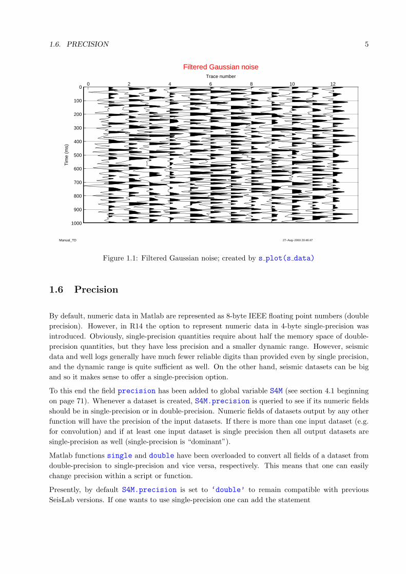
Test datasets for seismic data
• s data creates a seismic dataset consisting of 12 traces, 1000 ms long, of filtered random
noise as shown in Figure 1.1. It has one header: CDP.
• s data3d creates a 3-D seismic dataset; the only difference between a 2-D dataset and a 3-D
dataset is that the latter must have headers with location information — preferably inline
numbers and cross-line numbers. Consequently, the dataset output by s data3d has two
headers: iline no and xline no.
1.6. PRECISION 5
27−Aug−2003 20:46:47Manual_TD
0 2 4 6 8 10 120
100
200
300
400
500
600
700
800
900
1000
Tim
e (m
s)
Trace number
Filtered Gaussian noise
Figure 1.1: Filtered Gaussian noise; created by s plot(s data)
1.6 Precision
By default, numeric data in Matlab are represented as 8-byte IEEE floating point numbers (double
precision). However, in R14 the option to represent numeric data in 4-byte single-precision was
introduced. Obviously, single-precision quantities require about half the memory space of double-
precision quantities, but they have less precision and a smaller dynamic range. However, seismic
data and well logs generally have much fewer reliable digits than provided even by single precision,
and the dynamic range is quite sufficient as well. On the other hand, seismic datasets can be big
and so it makes sense to offer a single-precision option.
To this end the field precision has been added to global variable S4M (see section 4.1 beginning
on page 71). Whenever a dataset is created, S4M.precision is queried to see if its numeric fields
should be in single-precision or in double-precision. Numeric fields of datasets output by any other
function will have the precision of the input datasets. If there is more than one input dataset (e.g.
for convolution) and if at least one input dataset is single precision then all output datasets are
single-precision as well (single-precision is “dominant”).
Matlab functions single and double have been overloaded to convert all fields of a dataset from
double-precision to single-precision and vice versa, respectively. This means that one can easily
change precision within a script or function.
Presently, by default S4M.precision is set to ‘double’ to remain compatible with previous
SeisLab versions. If one wants to use single-precision one can add the statement
6
S4M.precision=’single’;
to file userDefaults4Seislab.m or create this file if it does not yet exist.
Alternatively, one can start a script with
presets
global S4M
S4M.precision=’single’;
Obviously, S4M.precision can be changed anywhere within a script or function. However, one
needs to keep in mind that this variable is only checked when a dataset is created. If one needs to
convert a double-precision dataset to single precision the function single needs to be used.
1.7 Displays
The ability to plot data is an important part of SeisLab. All figures use a labeling convention that
has proved useful in distinguishing figures create by different scripts or different runs of the same
script. Specifically, they write the name of the script that created the figure in the lower left corner
and the date and the time the script was started in the lower right corner. This means that figures
created by the same script have the same time-stamp. This feature is controlled by the value of
field figure labels of the global variable S4M. The default value is true. If this behavior is
not desired, e.g. because the figure is intended for a publication and should not have these labels,
S4M.figure labels should be set to false. More about the global structure S4M and its fields
can be found in the description of function presets in Chapter 4.1.
Figures have drop-down menus in addition to those provided by Matlab. Most depend on the type
for plot. However, a button Save plot is common to all of them. Attached to this button is a
drop-down menu with three choices to save the figure. The top one saves the figure as an EMF file
specifically for use in PowerPoint displays (EMF files can be edited in PowerPoint). The directory
to which this file is saved can be specified in field pp directory of global structure S4M (see Section
4.1 on pages 71 ff). The second choice is the JPEG format because of its universal use, and the
third choice, finally, saves the figure as an encapsulated Postscript (EPS) file, specifically for use in
LATEXdocuments. The directory to which EPS files are saved is specified in field eps directory
of global structure S4M.
In principle, Matlab allows saving figures in these and more formats. However, this requires a lot
of clicks.
1.8 Scripts with examples
The SeisLab distribution includes a folder “Examples”. It contains Matlab scripts that are intended
to illustrate the use of SeisLab. These scripts show sample implementations of various tasks a user
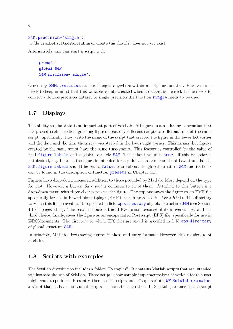
might want to perform. Presently, there are 12 scripts and a “superscript”, WF Seislab examples,
a script that calls all individual scripts — one after the other. In SeisLab parlance such a script
1.8. SCRIPTS WITH EXAMPLES 7
is a “Workflow”. In figures, the workflow name is displayed in the lower left corner above the
script name (see Figure 1.2). I highly recommend to run the work-flow script to check if SeisLab is
correctly installed.
31−Jul−2009 05:33:32WF_Seislab_examplesExamples4SeismicWigglePlots
1 3 5 7 9 110
100
200
300
400
500
600
700
800
900
1000
Trace number
Dataset
Example 11: Plot of two equally scaled datasets
1 3 5 7 9 110
100
200
300
400
500
600
700
800
900
1000
Trace number
0.5*Dataset (same scale)
Figure 1.2: A figure from script Examples4SeismicWigglePlots; the label in the lower left
corner shows that it has been run from workflow WF Seislab examples. The figure shows a
vertical line along the zero-deflection axis of most traces. This is an artifact that, more or less
frequently, shows up on paper copies of seismic wiggle plots; it can be prevented by including input
argument {‘quality’,‘high’} in function s wplot (for a discussion of keyword quality see
page 28).

8
Chapter 2
SEISMIC DATA
2.1 A brief look at some functions for seismic data
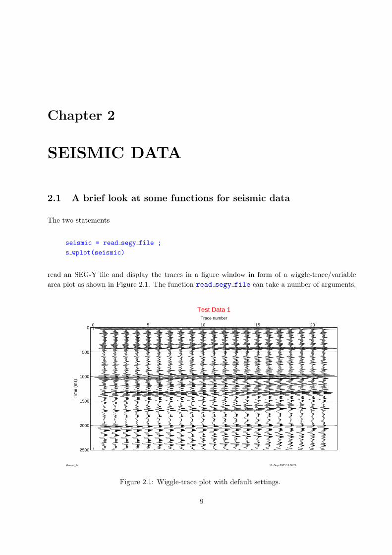
The two statements
seismic = read segy file ;
s wplot(seismic)
read an SEG-Y file and display the traces in a figure window in form of a wiggle-trace/variable
area plot as shown in Figure 2.1. The function read segy file can take a number of arguments.
11−Sep−2005 15:36:21Manual_1a
0 5 10 15 200
500
1000
1500
2000
2500
Trace number
Tim
e (m
s)
Test Data 1
Figure 2.1: Wiggle-trace plot with default settings.
9
10 CHAPTER 2. SEISMIC DATA
One of them, of course, is the file name; but if it is not given, a file selection box allows interactive
file selection.
The data read from the SEG-Y file are stored in the structure seismic. This structure is basically a
container which collects different pieces of data (seismic traces, headers, start time, sample interval,
etc.) under one name. The structure seismic is then input to the plot function s wplot (most
seismic-related functions start with “s ”, and the “w” in s wplot stands for wiggle — s cplot
makes seismic plots with amplitudes represented by color).
The function s wplot has one required argument, the name of the seismic dataset. All other
arguments are optional. Figure 2.1 shows the plot obtained with these defaults. The traces are
numbered sequentially. Because no title was specified explicitly the string in the field name of the
seismic dataset (in this example Test Data 1) is used as a default title.
Using some of the optional arguments, one can tailor the two statements to specific needs. For
example,
seismic data = read segy file(‘C:\Data\Test Data 2.sgy’,{‘times’,500,1500}, ...
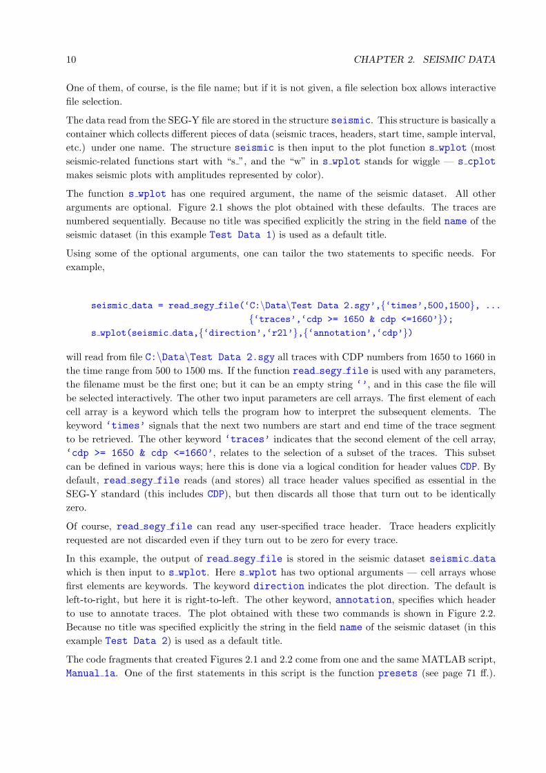
{‘traces’,‘cdp >= 1650 & cdp <=1660’});s wplot(seismic data,{‘direction’,‘r2l’},{‘annotation’,‘cdp’})
will read from file C:\Data\Test Data 2.sgy all traces with CDP numbers from 1650 to 1660 in
the time range from 500 to 1500 ms. If the function read segy file is used with any parameters,
the filename must be the first one; but it can be an empty string ‘’, and in this case the file will
be selected interactively. The other two input parameters are cell arrays. The first element of each
cell array is a keyword which tells the program how to interpret the subsequent elements. The
keyword ‘times’ signals that the next two numbers are start and end time of the trace segment
to be retrieved. The other keyword ‘traces’ indicates that the second element of the cell array,
‘cdp >= 1650 & cdp <=1660’, relates to the selection of a subset of the traces. This subset
can be defined in various ways; here this is done via a logical condition for header values CDP. By
default, read segy file reads (and stores) all trace header values specified as essential in the
SEG-Y standard (this includes CDP), but then discards all those that turn out to be identically
zero.
Of course, read segy file can read any user-specified trace header. Trace headers explicitly
requested are not discarded even if they turn out to be zero for every trace.
In this example, the output of read segy file is stored in the seismic dataset seismic data
which is then input to s wplot. Here s wplot has two optional arguments — cell arrays whose
first elements are keywords. The keyword direction indicates the plot direction. The default is
left-to-right, but here it is right-to-left. The other keyword, annotation, specifies which header
to use to annotate traces. The plot obtained with these two commands is shown in Figure 2.2.
Because no title was specified explicitly the string in the field name of the seismic dataset (in this
example Test Data 2) is used as a default title.
The code fragments that created Figures 2.1 and 2.2 come from one and the same MATLAB script,
Manual 1a. One of the first statements in this script is the function presets (see page 71 ff.).
2.1. A BRIEF LOOK AT SOME FUNCTIONS FOR SEISMIC DATA 11
11−Sep−2005 15:36:21Manual_1a
165016521654165616581660500
600
700
800
900
1000
1100
1200
1300
1400
1500
CDP numberT
ime
(ms)
Test Data 2
Figure 2.2: Wiggle-trace plot with traces labeled by CDP, increasing from right to left.
which sets a number of global variables, among them a plot label for the lower left corner of plots
and the date and the time the script was started. It is this date/time combination that is displayed
in the lower right corner of the plots. Consequently, all plots created by the script in a particular
run bear the same time stamp.
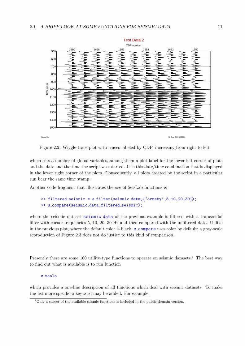
Another code fragment that illustrates the use of SeisLab functions is
>> filtered seismic = s filter(seismic data,{‘ormsby’,5,10,20,30});>> s compare(seismic data,filtered seismic);
where the seismic dataset seismic data of the previous example is filtered with a trapezoidal
filter with corner frequencies 5, 10, 20, 30 Hz and then compared with the unfiltered data. Unlike
in the previous plot, where the default color is black, s compare uses color by default; a gray-scale
reproduction of Figure 2.3 does not do justice to this kind of comparison.
Presently there are some 160 utility-type functions to operate on seismic datasets.1 The best way
to find out what is available is to run function
s tools
which provides a one-line description of all functions which deal with seismic datasets. To make
the list more specific a keyword may be added. For example,
1Only a subset of the available seismic functions is included in the public-domain version.
12 CHAPTER 2. SEISMIC DATA
11−Sep−2005 15:36:21Manual_1a
0 2 4 6 8 10 12500
600
700
800
900
1000
1100
1200
1300
1400
1500
Trace number
Tim
e (m
s)
Test Data 2 vs. filtered Test Data 2
Figure 2.3: Comparison of original (black) and filtered (red) seismic traces.
s tools seg
lists only those functions that deal with SEG-Y data files (the search is not case sensitive):
read segy file Read disk file in SEG-Y format
show segy header Output/Display EBCDIC header of SEG-Y file as ASCII
write segy file Write disk file in SEG-Y format
2.2. HEADERS 13
2.2 Headers
Trace headers (headers, for short) store trace-specific information such as offset, trace location, CDP
number, in-line number, cross-line number, etc. and play a major role in seismic data processing.
As mentioned above, when an SEG-Y file is read a number of headers are read by default; other
headers may be read as requested by input arguments of read segy file. Additional headers will
be added by certain functions: s align, for example, which aligns (flattens) an event on a seismic
section stores the shifts applied to each trace in a header value. This way the shifts can be undone
if necessary.
Headers are discussed again in the section on seismic datasets. As long as established functions are
used for their manipulation nothing needs to be known about the way they are stored in the seismic
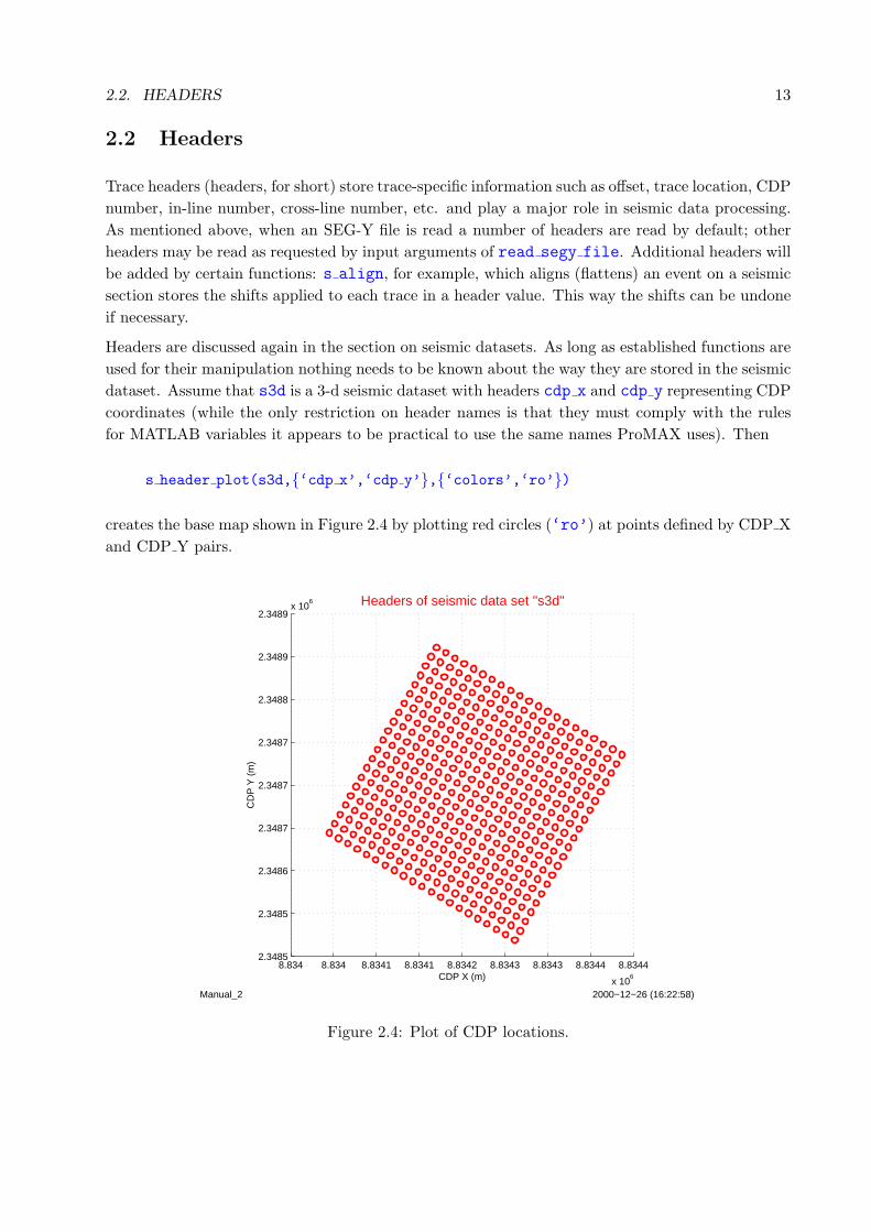
dataset. Assume that s3d is a 3-d seismic dataset with headers cdp x and cdp y representing CDP
coordinates (while the only restriction on header names is that they must comply with the rules
for MATLAB variables it appears to be practical to use the same names ProMAX uses). Then
s header plot(s3d,{‘cdp x’,‘cdp y’},{‘colors’,‘ro’})
creates the base map shown in Figure 2.4 by plotting red circles (‘ro’) at points defined by CDP X
and CDP Y pairs.
2000−12−26 (16:22:58)Manual_2
8.834 8.834 8.8341 8.8341 8.8342 8.8343 8.8343 8.8344 8.8344
x 106
2.3485
2.3485
2.3486
2.3487
2.3487
2.3487
2.3488
2.3489
2.3489x 10
6 Headers of seismic data set "s3d"
CDP X (m)
CD
P Y
(m
)
Figure 2.4: Plot of CDP locations.
14 CHAPTER 2. SEISMIC DATA
The same base map can be created by means of the standard Matlab plot commands
>> figure
>> plot(ds gh(s3d,‘cdp x’),ds gh(s3d,‘cdp y)’,‘ro’,‘LineWidth’,1.5)
>> xlabel([s gd(s3d,‘cdp x’),‘(’,s gu(s3d,‘cdp x’),‘)’])
>> ylabel([s gd(s3d,‘cdp y’),‘(’,s gu(s3d,‘cdp y’),‘)’])
>> title(’Headers of seismic data set "s3d"’,‘FontSize’,14,‘Color’,‘r’)
>> grid on
>> timeStamp
which is more tedious. It employs the functions
>> header values = ds gh(seismic,header mnemonic);
>> header units = s gu(seismic,header mnemonic);
>> header description = s gd(seismic,header mnemonic);
to retrieve, from seismic dataset seismic, a row vector of header values and a text strings with units
of measurement and a description, respectively, of the header with mnemonic header mnemonic
(header mnemonic is a character string).
Obviously, the header values could be extracted directly from the matrix seismic.headers and
units of measurement and header description from the cell array seismic.header info. How-
ever, using the above functions insulates a user from the need to know in what particular row of
seismic.headers and seismic.header info the requested information is stored. Also, if the
global variable S4M.case sensitive is set to 0 (false) — see start-up function presets (page 71)
— it does not matter if the header mnemonic specified is in lower case, upper case, capitalized, or
consists of any mixture of lower-case and upper-case characters. Incidentally, function ds gh has a
second, optional output argument; it is the appropriate row of cell matrix seismic.header info,
a three-element cell vector with the header mnemonic, the header’s units of measurement, and the
header description.
2.3 Description of seismic datasets
The seismic-related functions assume that a seismic dataset is represented by a structure which
— in addition to the actual seismic traces — contains necessary ancillary information in form of
required parameters, optional parameters, and headers. Parameters are pieces of information such
as start time, sample interval, etc. which pertain to all traces of the seismic dataset. Headers, on
the other hand, are trace-specific. They can vary from one trace to the next. Hence, each header
has a value for each trace. Seismic data proper are stored in a matrix whose columns represent
individual traces. In general, each row in this matrix represents a specific time. However, it is
also possible that each row represents a frequency or a depth. Hence, the term “time” is used in a
somewhat loose sense; it could also mean some other dimension. For this reason seismic datasets
have a field called units which defines the units of measurements. The default is ms.
The simplest seismic dataset can be created by the MATLAB statement
2.3. DESCRIPTION OF SEISMIC DATASETS 15
>> seismic = s convert(matrix,start time,sample interval)
where matrix denotes a matrix of seismic trace values, start time is the time of the first sample
and sample interval the sample interval. The resulting structure seismic has the nine fields
required of a seismic dataset. They are described below, and the description uses the following
variables
nsamp number of samples per trace
ntr number of traces per dataset
nh number of headers in the dataset
In this section the name seismic is used to refer to a seismic dataset. Thus, seismic.traces
denotes the field ‘traces’ of a seismic dataset.
• type type of dataset. For seismic data it is set to the string ‘seismic’. This field is
intended to allow interactive programs to identify quickly the type of dataset represented by
a particular structure; i.e. distinguish between seismic datasets, well logs, etc.
• tag an attribute that describes more clearly the kind of seismic datasets. Possible values are:
‘wavelet’, ‘impedance’, ‘reflectivity’, and the catch-all ‘unspecified’.
• name Name of the dataset; by default, for a dataset read from an SEG-Y file, it is the file
name.
• first Time (or frequency, or depth) associated with the first row of field ‘traces’.
• last Time (or frequency, or depth) associated with the last row of field ‘traces’.
• step Sample interval; obviously (last - first)/step +1 = nsamp.
• units Units of measurements for time (or frequency, or depth); examples are ‘ms’, ‘Hz’, ‘m’,
‘ft’.
• traces A matrix of numeric values with dimension nsamp by ntr. Each column of the field
traces represents a seismic trace.
• null Null value or no-data value. This value, in general NaN, is set by a function if some of
its output data in traces are not valid. This may happen if noise spikes have been removed,
if datasets with differing start times or end times are concatenated, etc. While it is common
to set to zero or to clip bad data (such as noise burst, data with excessive NMO stretch, etc.)
it is frequently more prudent to have a special value that identifies them as invalid. If there
are no invalid values then the field null is set to the empty matrix, []. If seismic.null
== 0 then either all data are valid or invalid data have simply been zeroed. When data are
written to an SEG-Y file (see write segy file) any NaNs are replaced by zeros.
In addition to the required fields seismic functions create and use a number of additional structure
fields. Most frequently used are:
16 CHAPTER 2. SEISMIC DATA
• headers A matrix of numeric header values with dimension nh by ntr. Each row of this
matrix represents the value of a particular header for each trace. Examples of such headers
are cdp, offset, etc.
• header info A cell array of strings with dimension nh by 3. Each row of this cell array lists
a header in terms of its mnemonic (first column), its units of measurement (second column),
and its description. Many headers, such as cdp, have no units of measurement; they have
‘n/a’ in column 2.
• history A four-column cell array with a “processing history”, i.e a list of the MATLAB
functions used to create the seismic dataset. Entries into this field are made automatically
by most processes unless this option is turned off (see description of the function presets).
• header null Null value or no-data value. This value, in general NaN, is set by a process if
some of its output data in headers are not valid. This may happen if datasets with differing
headers are concatenated (e.g. synthetics spliced into real data), etc. When headers are
written to an SEG-Y file any NaNs are be replaced by zeros.
• time One time value for each row of data matrix seismic.trace allowing non-uniformly
spaced data. This is generally used if seismic data have been converted from time to depth.
Furthermore there can be an arbitrary number of fields representing parameters
Below is an example of the simplest seismic dataset:
wavelet
type : ‘seismic’ Type of structure
tag : ‘wavelet’ Tag; more specific description of dataset
name : ‘Ormsby (zero-phase)’ Name
first : -40 Time of first sample
step : 4 Sample interval in msec
last : 40 Time of last sample in msec
units : ‘ms’ Units of measurement of time axis
traces : [21x1 double] One-column array with 21 entries
null : [ ] No null values
It represents an 80-ms wavelet with 4 ms sample interval and centered at time zero. While it may
be advantageous to have more information attached to the structure (for example the CDP or
in-line and cross-line number for which the wavelet was determined, or the processing history), this
is not required. However, even if no header is explicitly specified there is an implied pseudo-header
trace no that can be used like any other header. It is the sequential number of each trace and is
called pseudo-header since it is not attached to a specific trace; thus if one removes a trace from
a dataset the pseudo-header trace no of all traces following the one that was removed will be
decreased by one. “Real” headers of a trace, on the other hand, are not affected if one or more
traces are added or removed from a dataset.
The following example shows a more elaborate structure output by the function
read segy file discussed below which reads an SEG-Y file.
2.3. DESCRIPTION OF SEISMIC DATASETS 17
seismic
type : ‘seismic’ Type of structure
tag : ‘unspecified’ Tag; more specific description of dataset
name : ‘Test Data 3’ Name
line number : 1 Line number
traces per record : 48 Traces per record
first : 0 Time of first sample
step : 2 Sample interval in msec
last : 2000 Time of last sample in msec
units : ‘ms’ Units of measurement for the time axis
header info : [6x3 char] Descriptions of the header mnemonics
headers : [6x480 double] Header values
traces : [1001x480 double] Array (480 traces with 1001 samples, each)
history : 1x4 cell
null : [ ] No null values
The nine fields familiar from the first example indicate that the dataset consists of 480 traces
with 1001 samples each and a sample interval of 2 ms. Furthermore, there are the scalar fields
line number, traces per record and units which were take directly from the binary reel
header of the SEG-Y file. Of generally more interest are the trace headers. This seismic dataset
has six trace headers. Information about these trace headers is stored in the field header info.
They resemble the way ProMAX lists headers. The six header mnemonics as well as the associated
units of measurement and header descriptions are shown below.
Header mnemonic Units Header description
‘ds seqno’ ‘n/a’ ‘Trace sequence number within line’
‘ffid’ ‘n/a’ ‘Original Field record number’
‘o trace no’ ‘n/a’ ‘Trace sequence number within original field record’
‘cdp’ ‘n/a’ ‘CDP ensemble number’
‘seq cdp’ ‘n/a’ ‘Trace sequence number within CDP ensemble’
‘iline no’ ‘n/a’ ‘In-line number
None of these headers is associated with units of measurement and so all entries in the second
column are ‘n/a’. This would have been different if offsets or coordinates had been among the
headers. The most convenient and informative way of looking at the headers of seismic data
structure seismic is to execute the command
s header(seismic).
By default, read segy file initially reads 22 pre-set trace headers but then discards all those
whose values are zero for every trace. The first five headers listed above represent the remaining
non-zero preset trace headers. The sixth header (iline no) is a user-requested header read from
a user-defined byte location in the binary trace header of the SEG-Y file.
There are some mild restrictions on header names (they must satisfy all requirements placed on
MATLAB variables). Furthermore, it is highly recommended that the following header mnemonics
18 CHAPTER 2. SEISMIC DATA
Header mnemonics Header descriptions
cdp CDP ensemble number
offset Source-receiver distance
iline no In-line number
xline no Cross-line number
cdp x X-coordinate of CDP
cdp y Y-coordinate of CDP
sou x X coordinate of source
sou y Y coordinate of source
sou elev Surface elevation at source
rec x X coordinate of receiver
rec y Y coordinate of receiver
rec elev Receiver elevation
source Energy source point number
sou depth Source depth below surface
rec h2od Water depth at receiver
sou h2od Water depth at source
ffid Field file ID number
Table 2.1: Partial list of headers read from SEG-Y files; the complete list can be obtained with the
help read segy file command.
be used where applicable since they are expected to be present in certain functions. They correspond
to those used in ProMAX and, hence, ProMAX users should not find them difficult to remember.
The last field in the above structure is the history field. This is an optional field generally
created by all functions that create seismic datasets (e.g. read segy file) provided S4M.history
== true. Other functions append information to this field if it exists AND if S4M.history ==
true.
2.4 Operator and function overloading
Operator overloading refers to a facility in Matlab where operators such as ‘’+”, “-” or built-in
functions such as abs, sqrt, are given a special meaning in situations where they had none
before. An example is multiplication by a number of a Matlab structure such as a seismic dataset.
Thus 3*seismic (here and in the following seismic is a seismic dataset) would normally result
in an error message. However, in SeisLab the multiplication operator has been overloaded to make
this a meaningful statement for seismic datasets. In fact, 3*seismic means that the samples of the
seismic traces, i.e. the elements of the matrix seismic.traces, are multiplied by 3. In general,
the operator is applied to one field of the seismic dataset — the field traces. This is a convenience
feature meant to simplify interactive operations. Since it involves function calls it is somewhat
slower than direct operations on the field traces.
2.4. OPERATOR AND FUNCTION OVERLOADING 19
2.4.1 Overloaded operators
Unary plus (+) and minus (-)
+ seismic legal, but the same as seismic
- seismic means seismic.traces → - seismic.traces
Thus
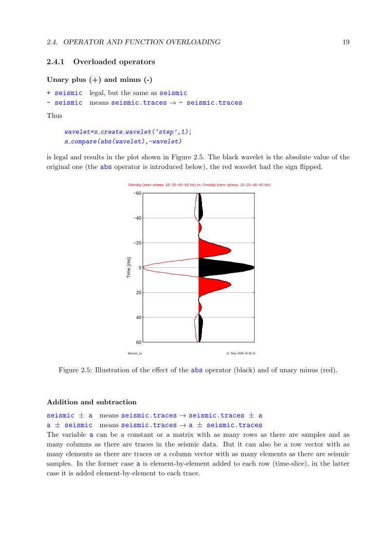
wavelet=s create wavelet(‘step’,1);
s compare(abs(wavelet),-wavelet)
is legal and results in the plot shown in Figure 2.5. The black wavelet is the absolute value of the
original one (the abs operator is introduced below), the red wavelet had the sign flipped.
11−Sep−2005 15:36:21Manual_1a
−60
−40
−20
0
20
40
60
Tim
e (m
s)
Ormsby (zero−phase, 10−20−40−60 Hz) vs. Ormsby (zero−phase, 10−20−40−60 Hz)
Figure 2.5: Illustration of the effect of the abs operator (black) and of unary minus (red).
Addition and subtraction
seismic ± a means seismic.traces → seismic.traces ± a
a ± seismic means seismic.traces → a ± seismic.traces
The variable a can be a constant or a matrix with as many rows as there are samples and as
many columns as there are traces in the seismic data. But it can also be a row vector with as
many elements as there are traces or a column vector with as many elements as there are seismic
samples. In the former case a is element-by-element added to each row (time-slice), in the latter
case it is added element-by-element to each trace.
20 CHAPTER 2. SEISMIC DATA
Multiplication
seismic * a means seismic.traces → seismic.traces * a
and is the same as a * seismic
The variable a can be a constant or a matrix with as many rows as there are samples and as
many columns as there are traces in the seismic data. But it can also be a row vector with as many
elements as there are traces or a column vector with as many elements as there are seismic samples.
In the former case each row (time-slice) is element-by-element multiplied by a, in the latter each
trace is element-by-element multiplied by a. An example is:
s=s data;
s1=s-s.traces(:,3);
s wplot(s1)
Division
seismic/a means seismic.traces → seismic.traces/a
The variable a should be a scalar (1×1 matrix).
Element-by-element division seismic ./ a means
seismic.traces → seismic.traces ./ a
The variable a can be a constant or a matrix with as many rows as there are samples and as
many columns as there are traces in the seismic data. But it can also be a row vector with as
many elements as there are traces or a column vector with as many elements as there are seismic
samples. In the former case each row (time-slice) is element-by-element divided by a, in the latter
each trace is element-by-element divided by a.
Thus, for example,
seismic scaled=seismic./max(seismic.traces);
normalizes traces so that the maximum of each trace is 1.
a ./ seismic means seismic.traces → a ./ seismic.traces
The variable a can be a constant or a matrix with as many rows as there are samples and as
many columns as there are traces in the seismic data. But it can also be a row vector with as
many elements as there are traces or a column vector with as many elements as there are seismic
samples. In the former case a is element-by-element divided by each row (time-slice), in the latter
case a is element-by-element divided by each trace.
Element-by-element power
seismicˆa means seismic.traces → seismic.traces.ˆa
2.4. OPERATOR AND FUNCTION OVERLOADING 21
2.4.2 Overloaded functions
Absolute value
abs(seismic) means seismic.traces → abs(seismic.traces)
An example of the use of the abs operation is shown in Figure 2.5, above.
Cumulative sum
cumsum(seismic) means seismic.traces → cumsum(seismic.traces)
Finite difference
diff(seismic) means seismic.traces → diff(seismic.traces)
Double precision
double(seismic) converts all numeric fields (’traces’, ’first’, ‘last’, ‘step’, etc.) of seismic dataset
seismic from single precision to double precision. It works completely analogously for well logs.
A dataset is not changed if the numeric fields are already in double precision.
Use function show precision to display the precision of the numeric fields of a dataset.
Exponential function
exp(seismic) means seismic.traces → exp(seismic.traces)
Imaginary part
imag(seismic) means seismic.traces → imag(seismic.traces)
Logarithm
log(seismic) means seismic.traces → log(seismic.traces)
For this operation to be valid the seismic traces must have positive samples only.
Real part
real(seismic) means seismic.traces → real(seismic.traces)
Sign
sign(seismic) means seismic.traces → sign(seismic.traces)
This means that positive samples are replaced by 1 and negative samples by -1. Zeros are not
changed.
22 CHAPTER 2. SEISMIC DATA
Single precision
single(seismic) converts all numeric fields (’traces’, ’first’, ‘last’, ‘step’, etc.) of seismic dataset
seismic from double precision to single precision. It works completely analogously for well logs.
Numeric fields of a dataset are not changed if they are already in single precision.
Use function show precision to display the precision of the numeric fields of a dataset.
2.5 Key tasks of seismic-data analysis
2.5.1 Input/Output of seismic data
SeisLab has several functions that allow importing and exporting of seismic data. The most im-
portant ones read and write files that follow the SEG-Y standard. The document describing this
standard can be found on the SEG web site (www.seg.org).
2.5.1.1 Input seismic data in SEG-Y format
Function read segy file reads seismic data and stores them in a seismic dataset — in the example
below it is called seismic. It has a single non-keyword argument: the filename. However, it is
generally not required. If the file name is not supplied, as in the example below,
seismic=read segy file
the function opens a file-selection window that allows interactive file selection.
Whenever a file is selected interactively the full path together with the name of the file selected is
printed to the screen. (The file selection function also remembers the directory from which the file
was copied and, on a subsequent request for an SEG-Y file, will open this directory right away.) If
read segy file is part of a MATLAB script this file name can be copied conveniently from the
MATLAB window to the script so that the file will be read without user intervention the next time
the script is run. File name and path name are also stored in S4M.filename and S4M.pathname,
i.e. in fields of the global structure S4M initialized in function presets. The file name without
extension is also written to the field name of the seismic dataset.
If the filename is known it can be included as the first argument.
seismic=read segy file(filename)
The filename filename should generally include the path. If it is invalid it is ignored and the
interactive file selection window will pop up. This latter behavior is important since a filename is
expected if any of the optional keyword-based input arguments are used.
Frequently, one needs only a subset of the seismic data. It is conceivable to read all the data and
then use function s select to select the subset required. However, this is not only more time
consuming; for large datasets one may encounter computer-memory limitations.
2.5. KEY TASKS OF SEISMIC-DATA ANALYSIS 23
The keyword times can be used to restrict the time range of the data read. Thus
seismic=read segy file(filename,{‘times’,start time,end time})
or
seismic=read segy file(filename,{‘times’,[start time,end time]})
reads only the seismic data for times beginning with start time and ending with end time. If
the requested range exceeds the range of the available data only the available data are read; for
example, if end time is greater than the time of the last sample of the seismic data then end time
is reduced to the actual end time of the data.
The keyword traces, which allows selection of the traces to read, offers more flexibility. It can be
used to read specific user-defined traces or use a logical expression to select the traces to read. For
example, statement
seismic=read segy file(filename,{‘traces’,1:2:10}) 1a
reads traces 1, 3, 5, 7, 9 of the SEG-Y file. The same traces can be selected via a logical expression.
seismic=read segy file(filename, ...
{‘traces’,‘mod(trace no,2)==1 & trace no < 10’}) 1b
The logical expression is contained in the string following the keyword traces. It uses the pseudo-
header (or implied header) trace no.2
The logical expression above contains only headers, functions of headers or constants. Special
care must be taken if the logical expression is to contain variables. Suppose one wants to use the
variables inc and last to select the increment in the trace number and the last possible trace.
For statement 1a this is trivial.
seismic=read segy file(filename,{‘traces’,1:inc:last})
The same is not true for statement 1b . It has to undergo some modifications since the variables
inc and last have to be converted to strings.
seismic=read segy file(filename, ...
{‘traces’,[’mod(trace no,‘,num2str(inc),‘)==1 & ...
trace no < ‘,num2str(last)]})
By default, read segy file reads those trace headers the SEG-Y standard document considers
significant.3 However, one might want to read additional headers — for example, those stored
2The pseudo-header trace no is not an explicitly defined header but it can be used like one. It represents the
sequential number of a seismic trace. For the first trace it has always the value 1.3Default headers and their byte locations are listed in the help section of read segy file.
24 CHAPTER 2. SEISMIC DATA
in unassigned byte locations. In order to read additional headers one needs to specify a header
mnemonic to be used for it in SeisLab, the first byte of its location in the binary trace header the
number of bytes, and the units of measurement; a brief description of the header is generally helpful.
Information of the additional headers to be read is supplied means of the keyword headers. This is
illustrated in the next example in which the inline number and the source-receiver distance (offset)
are read (actually, the offset is already read by default).
seismic = read segy file(‘’, ...
{‘headers’,{‘ILINE NO’,189,4,‘n/a’,‘In-line number’}, ...
{‘offset’,37,4,‘m’,‘Source-receiver distance’}})
In this case the file is interactively selected (the filename is empty). The inline number is read from
the 4 bytes beginning at byte locations 189 of the trace header and the offset from the 4 bytes be-
ginning at byte location 37; both are stored in the matrix of header values field seismic.headers
of the output dataset.
It is important to point out that headers read by default are treated differently than headers
explicitly requested by a user. Default headers are read but only retained if they are not identically
zero. Headers read because of a user request are always retained. For CDP data the offset is
generally zero; hence the default header offset is generally discarded. However, if it is explicitly
specified as in the example above it will be present — even if all its values are zero.
Reading 3-D data
Seismic 3-D data usually have headers that identify the geographic location of each trace in the data
volume. The most popular ones are inline number and cross-line number or cdp x and cdp y (the
x and y-coordinates of the CDP). Revision 2 of the SEG-Y standard suggests that the former be
stored in the binary trace header as 4 bytes beginning at header locations 189 and 193, respectively,
the latter two as 4 bytes beginning at header locations 181 and 185, respectively. The default used
by ProMAX is the other way around. In any case, one needs to find out where in the trace header
these numbers are stored. The following example assumes standard storage of inline and cross-line
numbers. Keyword ‘traces’ is used to select a volume of 99 by 101 traces centered around a
trace with inline number 334 and cross-line number 454 (e.g. a well location); they are less than
(or at most) 50 traces away from the center trace. The time range selected is 3100 to 4900 ms.
seis=read segy file(seisfilename,{‘headers’, ...
{‘ILINE NO’,189,4,‘n/a’,‘In-line number’}, ...
{‘XLINE NO’,193,4,‘n/a’,‘Cross-line number’}}, ...
{‘traces’,‘abs(iline no-334) < 50 & abs(xline no-454) =< 50’}, ...
{‘times’,3100,4900});
The resulting dataset has headers ‘XLINE NO’ and ‘ILINE NO’ in addition to those read by
default.4
Obviously, one can use logical expressions in various ways to specify traces one needs to read; e.g.
4By default, header mnemonics are not case-sensitive; hence, ‘ILINE NO’, for example, is equivalent to
‘iline no’. This behavior can be changed by setting field case sensitive of global variable S4M to false.
2.5. KEY TASKS OF SEISMIC-DATA ANALYSIS 25
{‘traces’,‘iline no >= 1000 & iline no <= 20000 & mod(xline no,2) == 0’}
selects the even cross-line numbers for all inline numbers between (and including) 1000 and 2000.
Binary-data formats
The SEG-Y standard allows five different formats for the numbers representing the seismic traces.
Presently, SeisLab supports only two of them — the legacy 4-byte IBM floating-point format and
the big-endian 4-byte IEEE floating-point format. A code number for the format used is stored in
bytes 25-26 of the binary file header, and an error will be thrown if the SEG-Y file had been created
with an unsupported format. Experience has shown that not all SEG-Y files have the correct format
code; hence, read segy file allows explicit specification of the format via keyword format. The
format specified via keyword format overrides the format code in the SEG-Y file; hence, it should
be used with caution.5
Zero time
In general, the first sample of every seismic trace in an SEG-Y file is associated with time 0, the
time of the shot (possibly with some corrections). However, each trace can be assigned a lag (delay)
which is stored in trace header bytes 109-110; it represents a lag time between shot and recording
start in ms. The value of lag is added to the start time of the seismic; hence, it can be used to
simulate non-zero start time of the seismic data. The existence of SEG-Y files with corrupted trace
headers made it necessary to provide an option to ignore the lag information. Hence, the need for
keyword ignoreshift which tells read segy file to ignore the shift parameter.
2.5.1.2 Output seismic data in SEG-Y format
Function write segy file which writes seismic data to a disk file in SEG-Y format has two
positional parameter, the dataset name and the filename; it latter is optional. If it is not supplied
or invalid a file-selection window will pop up to allow interactive filename selection. This is a simple
example which writes the seismic dataset seismic to disk.
write segy file(seismic)
NaNs in the data will be replaced by zeros.
If the start time is greater than zero then the data will be prepended by zeros to make the start
time zero. If the start time is less than zero (this is frequently the case for wavelets) the start time is
reset to zero and header lag is set to the actual start time. Consequently, when read segy file
reads this dataset it will restore the original start time. SEG-Y readers in other programs should
do the same.
One might wonder why positive and negative start times are treated differently. There used to be
SEG-Y readers that did not honor the lag header. This way, at least for positive start times, they
get the data correctly timed, and in SeisLab one can always use function s rm zeros to get rid of
the leading zeros.
5It is impossible to tell from a single number if it was read with the wrong format. However, a histogram of seismic
data read with the wrong format is markedly different from a histogram of data read with the correct format.
26 CHAPTER 2. SEISMIC DATA
By default the function writes the most important headers (the help section of write segy file
lists them together with their locations in the binary trace header). Those that are not found in
the dataset are deemed to be zero. If additional headers need to be stored they can be specified
via keyword headers. Specifically, for each header one needs to supply the mnemonic, the index
of the first byte of the trace header and the number of bytes it will occupy (either 2 or 4). The
following is an example.
write segy file(seismic,filename, ...
{‘headers’,{‘iline no’,189,4},{‘xline no’,193,4}});
The statement saves seismic dataset seismic in a file with filename filename. In addition to
the headers saved by default it stores header iline no in 4 bytes beginning at byte 189 in the
binary trace header and header xline no right after it (4 bytes beginning at byte 193 of the binary
trace header). These byte locations are actually the ones recommended in Revision 2 of the SEG-Y
format standard. Of course, headers with mnemonics iline no and xline no must be present in
dataset seismic.
Utility functions for SEG-Y files
Function show segy header is a little utility function that reads a disk file written in SEG-Y
format and outputs the EBCDIC header (converted to ASCII) to a file or prints it to the screen.
2.5.1.3 Proprietary data formats
Several companies with seismic-exploration software have developed their own formats for seismic
data files, usually text (ASCII) files. Most of these are used to exchange wavelets where shortcom-
ings of the SEG-Y format are felt most. Functions that read/write these files for several company
formats have been written and are discussed in the following.
Landmark Graphics
Function s wavelet from landmark reads wavelets in Landmark Graphics’ own format, and
s wavelet4landmark does the reverse; it writes wavelet in such a form that Landmark software
can read it.
Hampson-Russell
Function s wavelet from hampson russell reads wavelets from files in Hampson-Russell’s for-
mat. Function s wavelet4hampson russell writes a wavelet to a text file so that Hampson-
Russell software can read it.
Fugro Jason
Function s seismic4jason writes seismic data to an ASCII file in Jason, comma-separated format.
2.5. KEY TASKS OF SEISMIC-DATA ANALYSIS 27
2.5.2 Seismic-data display
Displays of seismic data play a fundamental role in seismic data analysis. SeisLab offers a num-
ber of plotting functions. Here they are grouped in categories such as wiggle plots, color plots,
combinations of wiggle and colors plots, plots of 3-D data, plots of spectra, headers, etc.
In addition to the “Save plot” menu item discussed above, seismic plots have a menu “Options”
with two menu items. The first, “Add scroll bars” (“Remove scroll bars”), allows one to add scroll
bars to a plot. When pressed for the first time this button creates scroll bars along the right-hand
side and along the bottom of the figure. The size of the scroll window needs to be selected by
the user. While the scroll bars are present the normal zoom function is unavailable. Clicking the
button again will remove the scroll bars. The scroll bars can be turned on and off repeatedly. This
way one can view a subset of the seismic data and move it horizontally and/or vertically.
The second menu item, “Turn tracking on” (“Turn tracking off”) refers to a feature where the
current position of the cursor and the seismic amplitude at the cursor location are displayed in the
lower left corner of the figure. This menu item toggles cursor tracking on and off. While cursor
tracking is on, the normal zoom function is unavailable. Initially, cursor tracking is turned off.
2.5.2.1 Wiggle plots
Function s wplot is the workhorse of wiggle-trace plotting. The folder “Examples” of the SeisLab
Distribution contains a script, Examples4SeismicWigglePlots.m with examples of its use. The
simplest form is
s wplot(seismic)
which plots the seismic dataset seismic. The vertical axis is annotated in time, the horizontal
axis in trace number (in fact, the pseudo header trace no). Figure 2.1, above, shows an example
of such a default plot.
To allow more general use the function does not abort if seismic is not a seismic dataset, but
rather a matrix. In this case the matrix columns are plotted as seismic traces in spike-format,
which is intended for the display of reflection coefficient series; the vertical and horizontal axes are
annotated as “Rows” and “Columns”, respectively.
The result of statement
s wplot(randn(50,12)) 2
is shown in Figure 2.6.
28 CHAPTER 2. SEISMIC DATA
12−Jul−2009 07:04:52Examples4SeismicWigglePlots
1 3 5 7 9 11
5
10
15
20
25
30
35
40
45
50
ColumnsR
ow
s
Figure 2.6: Plot created by statement 2 .
A large number of keyword-activated options allows control of many aspects of the plot. More
commonly used keywords are:
• {‘annotation’,string parameter} Specifies a header mnemonic for the annotation of
the horizontal axis. Default is the trace number ‘trace no’.
• {‘deflection’,numerical parameter} Amount of trace deflection. Default is 1.5.
• {‘direction’,string parameter} Possible values are ‘l2r’ (left to right) and ‘r2l’
(right to left). Default is ‘l2r’.
• {‘interpol’,string parameter} Interpolation to create a smooth plot. Options are
‘cubic’, ‘v5cubic’, and ‘linear’ (see Matlab function ‘’interp1”). Default is ‘v5cubic’.
• {‘orient’,string parameter}Orientation of plot. Options are ‘landscape’ and ‘portrait’.
Default is ‘portrait’ for ten or fewer traces and landscape for more than ten traces.
• {‘peak fill’,string parameter} Color of peak fill. Any MATLAB color is allowed.
Default is ‘k’ (black). An empty string parameter means no fill.
• {‘quality’,string parameter} This parameter controls how the seismic data are plotted.
If string parameter is ‘high’ or ‘draft’ the seismic data are displayed as wiggles; if
string parameter is ‘spike’ the seismic data are displayed as spikes. This latter option
is intended for the display of reflection coefficients.
For screen displays the difference between ‘high’ and ‘draft’ is generally immaterial.
However, hard copies, in particular on color printers, may show superfluous vertical lines
2.5. KEY TASKS OF SEISMIC-DATA ANALYSIS 29
when the figure had been created with the draft option. An example of such lines is shown
in Figure 1.2. In such cases the slower high-quality option ‘high’ should be used.
• {‘scale’,string parameter} Scaling of the data prior to plotting. Options are ‘yes’
(scale individual traces) and ‘no’ (do not scale individual traces; this preserves relative
amplitudes). Default is ‘no’. The scale factors actually used can be output and used to
scale subsequent plots. This can be used to create plots with several scale factors, and is
illustrated in Example 11 of script Examples4SeismicWigglePlots.
• {‘trough fill’,string parameter} Color of trough fill. Any Matlab color is allowed.
Default is the empty string implying no fill.
• {‘wiggle color’,string parameter} Color of wiggle. Any Matlab color is allowed. De-
fault is ‘k’ (black). An empty string parameter means no wiggle.
Examples of seismic plots are, for example, in Figures 2.1 and 2.2. Seismic traces can also be
plotted in different colors. This is illustrated in Figure 2.7
27−Nov−2004 22:16:45Colored_traces
0 2 4 6 8 10 120
100
200
300
400
500
600
700
800
900
1000
Trace number
Tim
e (m
s)
Test data
Figure 2.7: Plot of seismic traces in different colors.
The code that generated Figure 2.7 is shown below. It creates two copies, seismic1 and seismic2,
of the original seismic data. Traces 3, 5, and 10 of seismic1 are set to null values (NaN) and thus
will not be plotted. In seismic2 all traces except 3, 5, and 10 are set to null values. Then the two
datasets are plotted with seismic2 plotted in the same figure window as seismic1 (argument
{‘figure’,‘old’}).
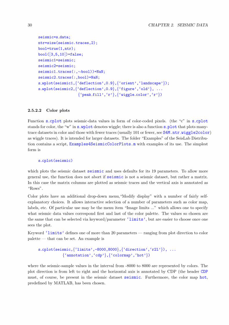
30 CHAPTER 2. SEISMIC DATA
seismic=s data;
ntr=size(seismic.traces,2);
bool=true(1,ntr);
bool([3,5,10 ])=false;
seismic1=seismic;
seismic2=seismic;
seismic1.traces(:,∼bool))=NaN;seismic2.traces(:,bool)=NaN;
s wplot(seismic1,{‘deflection’,0.9},{‘orient’,‘landscape’});s wplot(seismic2,{‘deflection’,0.9},{‘figure’,‘old’}, ...
{‘peak fill’,‘r’},{‘wiggle color’,‘r’})
2.5.2.2 Color plots
Function s cplot plots seismic-data values in form of color-coded pixels. (the “c” in s cplot
stands for color, the “w” in s wplot denotes wiggle; there is also a function s plot that plots many-
trace datasets in color and those with fewer traces (usually 101 or fewer, see S4M.ntr wiggle2color)
as wiggle traces). It is intended for larger datasets. The folder “Examples” of the SeisLab Distribu-
tion contains a script, Examples4SeismicColorPlots.m with examples of its use. The simplest
form is
s cplot(seismic)
which plots the seismic dataset seismic and uses defaults for its 19 parameters. To allow more
general use, the function does not abort if seismic is not a seismic dataset, but rather a matrix.
In this case the matrix columns are plotted as seismic traces and the vertical axis is annotated as
“Rows”.
Color plots have an additional drop-down menu,“Modify display” with a number of fairly self-
explanatory choices. It allows interactive selection of a number of parameters such as color map,
labels, etc. Of particular use may be the menu item “Image limits ...” which allows one to specify
what seismic data values correspond first and last of the color palette. The values so chosen are
the same that can be selected via keyword/parameter ‘limits’, but are easier to choose once one
sees the plot.
Keyword ‘limits’ defines one of more than 20 parameters — ranging from plot direction to color
palette — that can be set. An example is
s cplot(seismic,{‘limits’,-8000,8000},{‘direction’,‘r2l’}), ...
{‘annotation’,‘cdp’},{‘colormap’,‘hot’})
where the seismic-sample values in the interval from -8000 to 8000 are represented by colors. The
plot direction is from left to right and the horizontal axis is annotated by CDP (the header CDP
must, of course, be present in the seismic dataset seismic. Furthermore, the color map hot,
predefined by MATLAB, has been chosen.
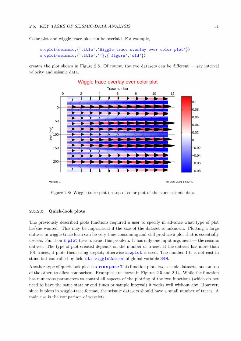
2.5. KEY TASKS OF SEISMIC-DATA ANALYSIS 31
Color plot and wiggle trace plot can be overlaid. For example,
s cplot(seismic,{‘title’,‘Wiggle trace overlay over color plot’})s wplot(seismic,{‘title’,‘’},{‘figure’,‘old’})
creates the plot shown in Figure 2.8. Of course, the two datasets can be different — say interval
velocity and seismic data.
−0.08
−0.06
−0.04
−0.02
0
0.02
0.04
0.06
0.08
0.1
30−Jun−2001 14:53:40Manual_1
Trace number
Tim
e (m
s)
Wiggle trace overlay over color plot
0 2 4 6 8 10 12
0
50
100
150
200
Figure 2.8: Wiggle trace plot on top of color plot of the same seismic data.
2.5.2.3 Quick-look plots
The previously described plots functions required a user to specify in advance what type of plot
he/she wanted. This may be impractical if the size of the dataset is unknown. Plotting a large
dataset in wiggle-trace form can be very time-consuming and still produce a plot that is essentially
useless. Function s plot tries to avoid this problem. It has only one input argument — the seismic
dataset. The type of plot created depends on the number of traces. If the dataset has more than
101 traces, it plots them using s cplot; otherwise s wplot is used. The number 101 is not cast in
stone but controlled by field ntr wiggle2color of global variable S4M.
Another type of quick-look plot is s compare This function plots two seismic datasets, one on top
of the other, to allow comparison. Examples are shown in Figures 2.5 and 2.14. While the function
has numerous parameters to control all aspects of the plotting of the two functions (which do not
need to have the same start or end times or sample interval) it works well without any. However,
since it plots in wiggle-trace format, the seismic datasets should have a small number of traces. A
main use is the comparison of wavelets.
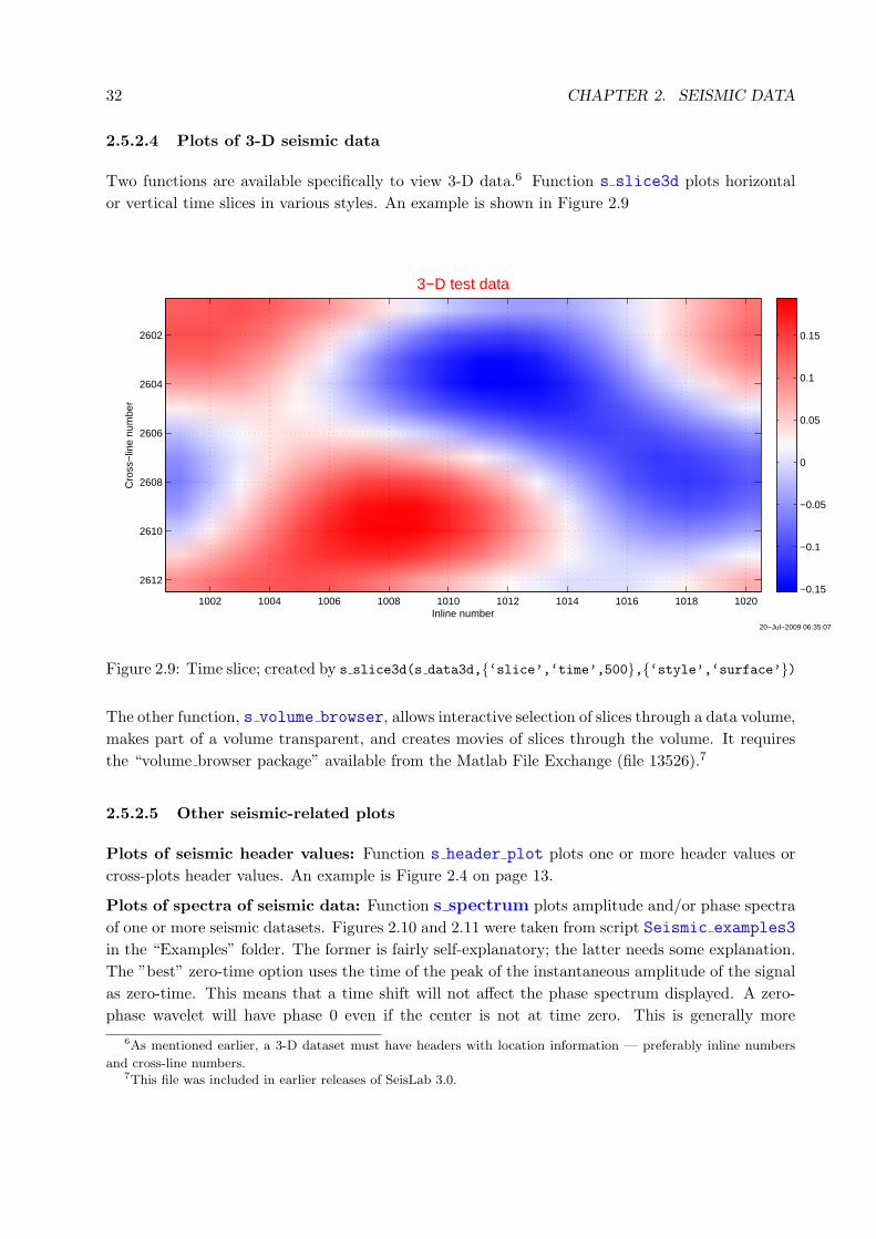
32 CHAPTER 2. SEISMIC DATA
2.5.2.4 Plots of 3-D seismic data
Two functions are available specifically to view 3-D data.6 Function s slice3d plots horizontal
or vertical time slices in various styles. An example is shown in Figure 2.9
20−Jul−2009 06:35:07
Inline number
Cro
ss−
line
num
ber
3−D test data
1002 1004 1006 1008 1010 1012 1014 1016 1018 1020
2602
2604
2606
2608
2610
2612−0.15
−0.1
−0.05
0
0.05
0.1
0.15
Figure 2.9: Time slice; created by s slice3d(s data3d,{‘slice’,‘time’,500},{‘style’,‘surface’})
The other function, s volume browser, allows interactive selection of slices through a data volume,
makes part of a volume transparent, and creates movies of slices through the volume. It requires
the “volume browser package” available from the Matlab File Exchange (file 13526).7
2.5.2.5 Other seismic-related plots
Plots of seismic header values: Function s header plot plots one or more header values or
cross-plots header values. An example is Figure 2.4 on page 13.
Plots of spectra of seismic data: Function s spectrum plots amplitude and/or phase spectra
of one or more seismic datasets. Figures 2.10 and 2.11 were taken from script Seismic examples3
in the “Examples” folder. The former is fairly self-explanatory; the latter needs some explanation.
The ”best” zero-time option uses the time of the peak of the instantaneous amplitude of the signal
as zero-time. This means that a time shift will not affect the phase spectrum displayed. A zero-
phase wavelet will have phase 0 even if the center is not at time zero. This is generally more
6As mentioned earlier, a 3-D dataset must have headers with location information — preferably inline numbers
and cross-line numbers.7This file was included in earlier releases of SeisLab 3.0.
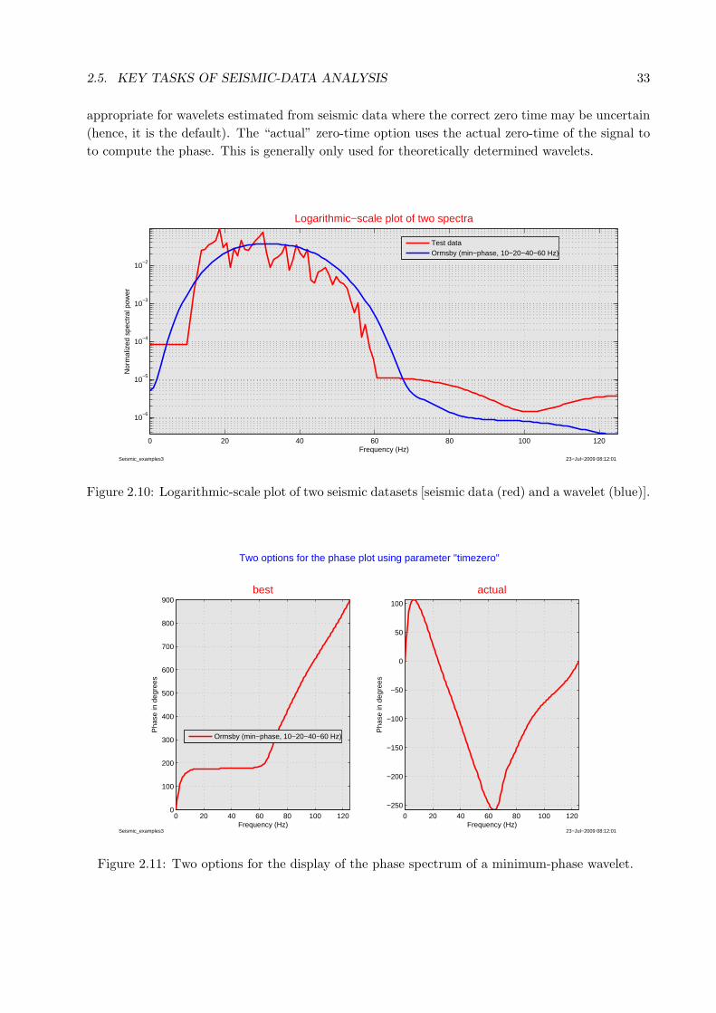
2.5. KEY TASKS OF SEISMIC-DATA ANALYSIS 33
appropriate for wavelets estimated from seismic data where the correct zero time may be uncertain
(hence, it is the default). The “actual” zero-time option uses the actual zero-time of the signal to
to compute the phase. This is generally only used for theoretically determined wavelets.
23−Jul−2009 08:12:01Seismic_examples3
0 20 40 60 80 100 120
10−6
10−5
10−4
10−3
10−2
Frequency (Hz)
Nor
mal
ized
spe
ctra
l pow
er
Logarithmic−scale plot of two spectra
Test dataOrmsby (min−phase, 10−20−40−60 Hz)
Figure 2.10: Logarithmic-scale plot of two seismic datasets [seismic data (red) and a wavelet (blue)].
23−Jul−2009 08:12:01Seismic_examples3
0 20 40 60 80 100 1200
100
200
300
400
500
600
700
800
900
Frequency (Hz)
Pha
se in
deg
rees
best
Ormsby (min−phase, 10−20−40−60 Hz)
Ormsby (min−phase, 10−20−40−60 Hz)
Two options for the phase plot using parameter "timezero"
0 20 40 60 80 100 120
−250
−200
−150
−100
−50
0
50
100
Frequency (Hz)
Pha
se in
deg
rees
actual
Figure 2.11: Two options for the display of the phase spectrum of a minimum-phase wavelet.
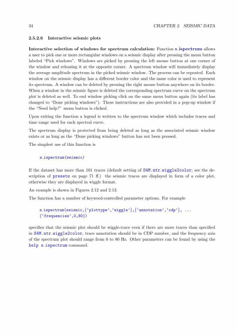
34 CHAPTER 2. SEISMIC DATA
2.5.2.6 Interactive seismic plots
Interactive selection of windows for spectrum calculation: Function s ispectrum allows
a user to pick one or more rectangular windows on a seismic display after pressing the menu button
labeled “Pick windows”. Windows are picked by pressing the left mouse button at one corner of
the window and releasing it at the opposite corner. A spectrum window will immediately display
the average amplitude spectrum in the picked seismic window. The process can be repeated. Each
window on the seismic display has a different border color and the same color is used to represent
its spectrum. A window can be deleted by pressing the right mouse button anywhere on its border.
When a window in the seismic figure is deleted the corresponding spectrum curve on the spectrum
plot is deleted as well. To end window picking click on the same menu button again (its label has
changed to “Done picking windows”). These instructions are also provided in a pop-up window if
the “Need help?” menu button is clicked.
Upon exiting the function a legend is written to the spectrum window which includes traces and
time range used for each spectral curve.
The spectrum display is protected from being deleted as long as the associated seismic window
exists or as long as the “Done picking windows” button has not been pressed.
The simplest use of this function is
s ispectrum(seismic)
If the dataset has more than 101 traces (default setting of S4M.ntr wiggle2color; see the de-
scription of presets on page 71 ff.) the seismic traces are displayed in form of a color plot,
otherwise they are displayed in wiggle format.
An example is shown in Figures 2.12 and 2.13.
The function has a number of keyword-controlled parameter options. For example
s ispectrum(seismic,{‘plottype’,‘wiggle’},{‘annotation’,‘cdp’}, ...
{‘frequencies’,0,80})
specifies that the seismic plot should be wiggle-trace even if there are more traces than specified
in S4M.ntr wiggle2color, trace annotation should be in CDP number, and the frequency axis
of the spectrum plot should range from 0 to 80 Hz. Other parameters can be found by using the
help s ispectrum command.
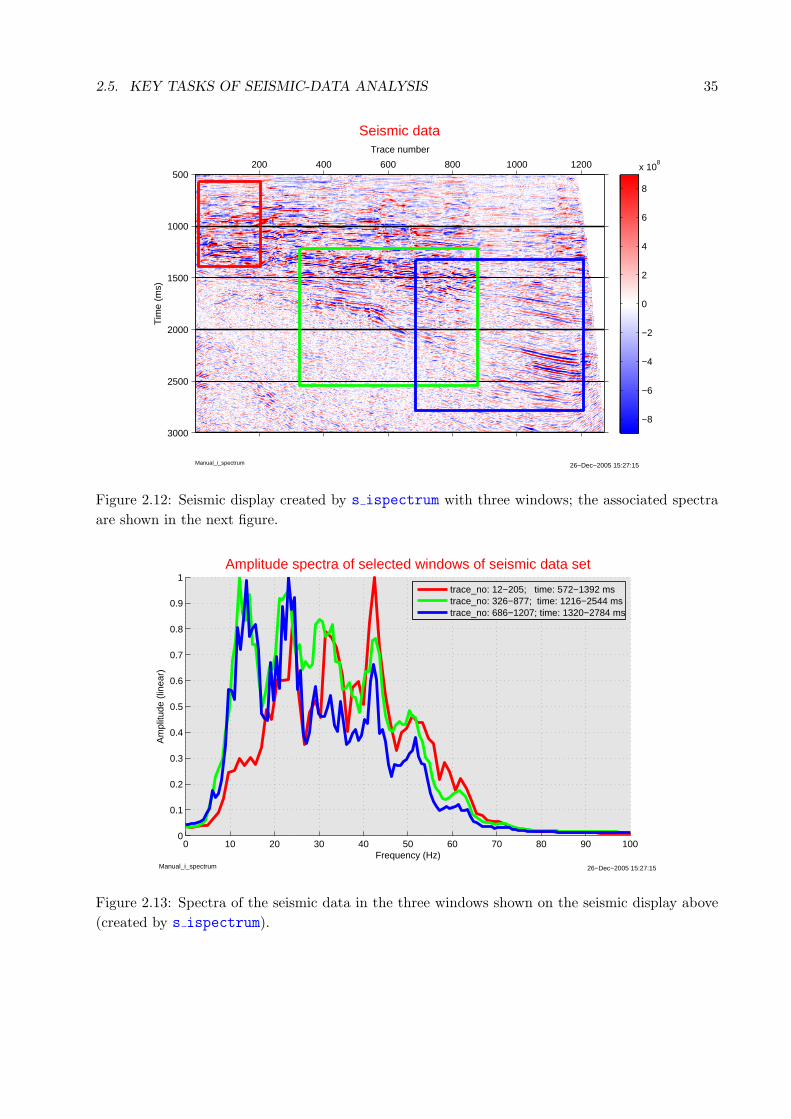
2.5. KEY TASKS OF SEISMIC-DATA ANALYSIS 35
26−Dec−2005 15:27:15Manual_i_spectrum
Trace numberT
ime
(ms)
Seismic data
200 400 600 800 1000 1200
500
1000
1500
2000
2500
3000
−8
−6
−4
−2
0
2
4
6
8
x 108
Figure 2.12: Seismic display created by s ispectrum with three windows; the associated spectra
are shown in the next figure.
26−Dec−2005 15:27:15Manual_i_spectrum
0 10 20 30 40 50 60 70 80 90 1000
0.1
0.2
0.3
0.4
0.5
0.6
0.7
0.8
0.9
1
Frequency (Hz)
Am
plitu
de (
linea
r)
Amplitude spectra of selected windows of seismic data set
trace_no: 12−205; time: 572−1392 mstrace_no: 326−877; time: 1216−2544 mstrace_no: 686−1207; time: 1320−2784 ms
Figure 2.13: Spectra of the seismic data in the three windows shown on the seismic display above
(created by s ispectrum).
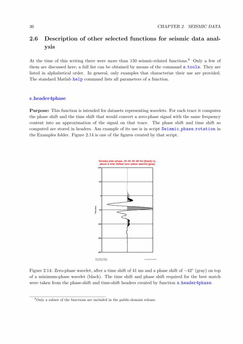
36 CHAPTER 2. SEISMIC DATA
2.6 Description of other selected functions for seismic data anal-
ysis
At the time of this writing there were more than 150 seismic-related functions.8 Only a few of
them are discussed here; a full list can be obtained by means of the command s tools. They are
listed in alphabetical order. In general, only examples that characterize their use are provided.
The standard Matlab help command lists all parameters of a function.
s header4phase
Purpose: This function is intended for datasets representing wavelets. For each trace it computes
the phase shift and the time shift that would convert a zero-phase signal with the same frequency
content into an approximation of the signal on that trace. The phase shift and time shift so
computed are stored in headers. Am example of its use is in script Seismic phase rotation in
the Examples folder. Figure 2.14 is one of the figures created by that script.
22−Sep−2009 16:54:06WF_Seislab_examplesSeismic_phase_rotation
−100
−50
0
50
100
150
200
Tim
e (m
s)
Ormsby (min−phase, 10−20−40−60 Hz) [black] vs.phase & time shifted zero−phase wavelet [gray]
Figure 2.14: Zero-phase wavelet, after a time shift of 41 ms and a phase shift of −42◦ (gray) on top
of a minimum-phase wavelet (black). The time shift and phase shift required for the best match
were taken from the phase-shift and time-shift headers created by function s header4phase.
8Only a subset of the functions are included in the public-domain release.
2.6. DESCRIPTION OF OTHER SELECTED FUNCTIONS FOR SEISMIC DATA ANALYSIS37
s align
Purpose: This function flattens an event (e.g. a reflector) by aligning it on all traces to that of a
reference trace.
s append
Purpose: This function appends one seismic data set to another to form one single seismic data
structure. The simplest form is
seisout = s append(seisin1,seisin2);
where seisout contains the traces of seisin1 followed by the traces of seisin2. Times of the
first and the last sample of seisout are defined by:
seisout.first = min(seisin1.first,seisin2.first);
seisout.last = max(seisin1.first,seisin2.first).
Likewise the headers of seisout are the union of the headers of seisin1 and seisin2. Times
in one input dataset that are not present in the other are set to the trace null value in the output
dataset. If the trace null value is NaN the field seisout.null is set to NaN. Similarly, headers
absent in one dataset but present in the other are set to the header null value which may differ
from the trace null value. If the header null value is NaN the field seisout.header null is set to
NaN.
Other ways of handling the combination of the two datasets can be specified by keyword-controlled
input arguments.
s attributes
Purpose: For each trace of the input dataset this function computes attributes of the seismic
traces and stores them in header(s). The attributes computed are:
• Average absolute amplitude of each trace
• Maximum absolute amplitude of each trace
• Median of absolute amplitudes of each trace
• Absolute value of trace minimum of each trace
• L2 norm each trace
• Maximum of each trace
• Mean of each trace
• Median of each trace
38 CHAPTER 2. SEISMIC DATA
• Minimum of each trace
• Minimum of the absolute values of each trace
• RMS amplitude of each trace
The simplest form is
s attributes(seismic)
which computes and prints to the screen a summary of the attributes. If an output dataset is
provided, the attributes are added to the trace headers or they replace already existing headers
with the same name.
seismic = s attributes(seismic)
It is also possible to specify that only a subset of the attributes be computed.
seismic=s attributes(seismic,{‘action’,‘add ne’},{‘attributes’,‘max’,‘rms’});
In this example s attributes computes the maximum amplitude and the RMS amplitude of each
trace, stores this information in headers named max and rms, respectively, and outputs the input
dataset with the additional headers.
s check
Purpose: This functions checks a seismic data structure for formal errors such as inconsistencies,
missing required fields, etc. It takes only one argument, the dataset to be checked. An example is
s check(seismic)
which checks for errors of the structure seismic; if, indeed, errors are found, it will print messages
explaining them. Otherwise, the message No formal errors found in ‘‘seismic’’ will be
printed.
It is expected that every seismic-related function listed in this manual will pass this consistency
test; however, users may modify structures outside of these functions and, if these changes are more
severe, checking if they violate any formal requirements may be appropriate.
s convert
Purpose: This function converts a matrix into a minimal seismic data structure. An example is
seismic=s convert(randn(201,20),0,4)
2.6. DESCRIPTION OF OTHER SELECTED FUNCTIONS FOR SEISMIC DATA ANALYSIS39
which converts a 200 by 20 matrix of random, normally distributed noise into a 20-trace seismic
dataset with start time 0 and 4 ms sample interval. The result is the following seismic dataset
seismic =type: ‘seismic’
tag: ‘unspecified’
name: ‘’
first: 0
step: 4
last: 800
units: ‘ms’
traces: [200x20 double]
null: []
history: {‘12-Jul-2007 21:15:41 ‘ [799] ‘S CONVERT’ []}
Since no content has been specified for the history field it is set by default (since S4M.history
== true). The same is true for the fields units, tag, and name.
s convolve
Purpose: seisout = s convolve(seisin1,seisin2) convolves the two seismic datasets and
outputs the result. There are optional input arguments that allow specification of various aspects
of the operation. The two seismic datasets must satisfy the following restrictions: either both
datasets have the same number of traces (in this case corresponding traces of the two datasets are
convolved) or at least one of the datasets must consist of one trace only (in this case it is convolved
with all the traces of the other dataset. As a result the number of traces in seisout is equal to
the number of traces of the larger input dataset (in terms of traces). Consequently, the headers
of this larger dataset are passed on to the output dataset. If both datasets have the same number
of traces the headers of the first datasets are copied to the output dataset. This behavior can be
changed by use of the keyword header
• {‘header’,numerical parameter} Select input dataset to supply the headers for seisout.
Possible values are 1 and 2. Default is 1.
If one of the datasets consists of one trace and the other has more than one trace the headers of
the larger datasets are copied to the output dataset.
s correlate
Purpose: seis = s correlate(seis1,seis2) performs a crosscorrelation of the traces of the
two seismic data sets and outputs the result. Optional, keyword-controlled arguments allow speci-
fication of various aspects of the operation. The default is that each trace of the second dataset is
correlated with each trace of the first dataset. The output dataset has two headers (default: ‘seis1’
40 CHAPTER 2. SEISMIC DATA
and ‘seis2’) which, for each output trace indicate which input trace of the first and of the second
dataset was used for its calculation.
Alternatively, each trace of the second dataset can be correlated with the corresponding trace of
the first dataset. In this latter case the two seismic datasets must have the same number of traces.
As a result the number of traces in seisout is equal to the number of traces of the input datasets.
The headers of the first input dataset are passed on to the output data set.
s create qfilter
Purpose: This function creates constant-Q absorption filters. For a range of t and Q values these
filters have an amplitude spectrum
A(f) = exp
(−πft
Q
)and a phase spectrum that ensures that they are causal.
This function is used, for example, in script Seismic examples2.
s create wavelet
Purpose: This function computes a Ricker wavelet or a wavelet with trapezoidal amplitude spec-
trum. In the latter case the phase options are minimum-phase, zero-phase, and maximum-phase.
An example is
wav=s create wavelet({‘type’,‘min-phase’},{‘frequencies’,10,10,40,60}, ...
{‘step’,2})
which creates a minimum-phase wavelet with 2 ms sample interval; the amplitude spectrum has
corner frequencies of 10, 10, 40, and 50 Hz.
This function is used, for example, in script Seismic examples1.
s filter
Purpose: This function filters a seismic dataset using an Ormsby band-pass filter (trapezoidal
amplitude spectrum).
This function is used, for example, in script Seismic examples1.
s header
Purpose: This function displays or manipulates trace headers of a seismic dataset. It can be used
to add, replace, display, rename, or delete trace headers (mnemonics, descriptions, and values).
2.6. DESCRIPTION OF OTHER SELECTED FUNCTIONS FOR SEISMIC DATA ANALYSIS41
The simplest use is
s header(seismic);
which prints to screen the name of every trace header together with its minimum value, maximum
value, minimum and maximum trace-to-trace increment, units of measurement and description.
The general usage of the function is:
seismic = s header(seismic,action,mnem,values,units,description)
The second argument, action, specifies the action taken by the function. Possible values of action
are:
• add Add header with mnemonic mnem to seismic dataset. Error if it already exists.
• add ne Add header with mnemonic mnem to seismic data set. Replaces it if it already exists.
• replace Replaces header with mnemonic mnem in seismic data set. Error if it already exists.
• delete Delete header with mnemonic(s) mnem in seismic dataset. Error if it header does
(headers do) not exist.
• delete ne Delete header(s) with mnemonic(s) mnem in seismic dataset. No error if it one or
more header does (headers do) not exist.
• keep Keep header(s) with mnemonic(s) mnem in seismic dataset; delete all others. Error if
there is not ar least one header to delete.
• keep ne Keep header(s) with mnemonic(s) mnem in seismic dataset; delete all others. No
error if it one or more header does (headers do) not exist.
• rename Rename header mnemonic, keep everything else the same
• list Print a short list: for specified header mnemonic(s) it lists minimum and maximum
value, smallest and greatest trace-to-trace change, units of measurement, and header descrip-
tion. This is the default that is being used if the seismic dataset is the only input argument.
s header math
Purpose: This function manipulates trace headers of a seismic dataset. It can be used to add or
replace trace headers by arithmetic manipulation of existing headers. As usual, the pseudo-header
“trace no” is implicitly present. An example of its use is:
seismic = s header math(seismic,‘add’,‘offset=sqrt((sou x-rec x)̂2 + ...
(sou y-rec y)̂2)’,‘m’,‘Source-receiver offset’)
which computes a new header, offset, from the source and receiver coordinates. These coordinates
must, of course, be headers of dataset seismic.
42 CHAPTER 2. SEISMIC DATA
s history
Purpose: This function manipulates the processing history as stored in the field history. The
simplest use is s history(seismic) which prints to screen the contents of the history field of
dataset seismic.
ds header sort
Purpose: This function sorts header value(s) of seismic data and pseudo-wells and outputs an
index vector (sorting can be performed in increasing or decreasing order). This index vector can
be used to sort seismic traces or pseudo-wells by header values.
Assume the traces of dataset wavelets are wavelets estimated for a number of traces and/or time
intervals and that the coefficient of correlation between the synthetic and the seismic is stored in
header cc coefficient (see function s wavextra). The following code segment will find and
plot the five wavelets with the highest correlation coefficient.
index=ds header sort(wavelets,{‘headers’,‘cc coefficient’}, ...
{‘sortdir’,‘decreasing’});bestwavelets=s select(wavelets,{‘traces’,index(1:5)});s wplot(bestwavelets)
s principal components
Purpose: This function computes principal components of the input dataset. Let sj(t) denote J
seismic traces. Then the first principal component is the function p1(t) which minimizes
J∑j=1
[sj(t)− cj1p1(t)]2
with appropriately chosen scale factors cj,1 (the function p1(t) is usually normalized to unit energy).
The first principal component p1(t) can be regarded as the single seismic trace that “best represents”
the J different seismic traces sj(t). It is easy to show that the first principal component is nothing
but a weighted stack of all the seismic traces (the weights may turn out be positive or negative).
It should be noted that the minimization condition above is not generally used to compute the
principal components; this is done via a Singular Value Decomposition of the matrix of seismic
traces.
The general representation of the seismic traces in terms of the principal components, pk, is
sj(t) =∑k
cjkpk(t) (2.1)
If the sum includes all principal components then the equal sign is appropriate. However, frequently
it is desirable to include only the first few ones.
The function s principal components has three possible outputs that can be selected via key-
word output.
2.6. DESCRIPTION OF OTHER SELECTED FUNCTIONS FOR SEISMIC DATA ANALYSIS43
1. a new dataset consisting of one or more of the principal components of the input dataset; i.e.,
the pk(t) for a user-specified range of k values.
2. a dataset where each of the input traces is represented by one or more of the principal
components; i.e., the sum in Eq. (2.1) over a user-specified range of k values.
3. the coefficients cjk in Eq. (2.1).
An example, with all the default parameters, is
pcs = s principal components(seismic);
The output dataset pcs has as many traces as the input data set but each trace is a scaled version
of the first principal component of the traces of dataset seismic, i.e. the j-th trace of the output
dataset is cj1p1(t) where cj,1 is the coefficient in Eq. (2.1), and p1(t) is the first principal component.
The statement
pcs=s principal components(seismic,{‘index’,1:3});
creates a dataset pcs where each trace is an approximation of the corresponding trace of the input
dataset by means of the first 3 principal components (this assumes that the dataset seismic has at
least 3 traces). Obviously, there are as many output traces as there are input traces. An example
from script Seismic principal components in the examples-folder is shown in Figure 2.15. The
difference between the two seismic plots on the left is the contribution that would have come from
principal components 4 to 12. An interesting feature is the fact that the difference is noticeably
larger for the first and last trace. This is due to the fact that the seismic traces have a certain
degree of continuity. There are fewer traces similar to the outermost traces; hence, the latter have
less influence on the shape of the first few principal components.
Assume the seismic dataset seismic consists of 7 traces.
seis1 4=s principal components(seismic,{‘components’,1:4});seis5 7=s principal components(seismic,{‘components’,5:7});error=max(seismic.traces-(seis1 4.traces+seis5 7.traces))
Then the traces of seis1 4 (the seismic data represented by the first 4 principal components)
added to the traces of seis5 7 (the seismic data represented by the last 3 principal components)
produce the traces of the original input data. In theory, the 7-component vector error should be
zero. In practice, due to rounding errors, its elements are generally non-zero but very small.
On the other hand, if the principal components are requested, the statement
pcs=s principal components(seismic,{‘output’,‘pc});
produces a seismic dataset with only one trace, the first principal component s(t) as defined above
— regardless of the number of input traces.
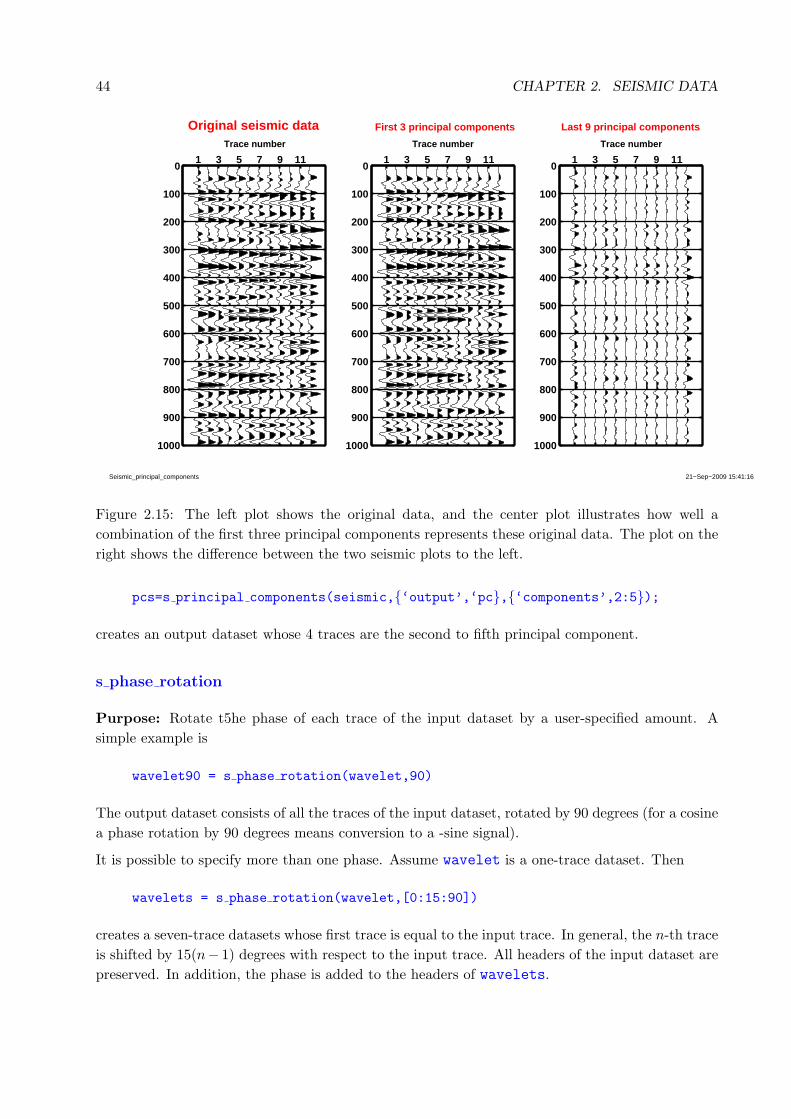
44 CHAPTER 2. SEISMIC DATA
21−Sep−2009 15:41:16Seismic_principal_components
1 3 5 7 9 110
100
200
300
400
500
600
700
800
900
1000
Trace number
Original seismic data
1 3 5 7 9 110
100
200
300
400
500
600
700
800
900
1000
Trace number
First 3 principal components
1 3 5 7 9 110
100
200
300
400
500
600
700
800
900
1000
Trace number
Last 9 principal components
Figure 2.15: The left plot shows the original data, and the center plot illustrates how well a
combination of the first three principal components represents these original data. The plot on the
right shows the difference between the two seismic plots to the left.
pcs=s principal components(seismic,{‘output’,‘pc},{‘components’,2:5});
creates an output dataset whose 4 traces are the second to fifth principal component.
s phase rotation
Purpose: Rotate t5he phase of each trace of the input dataset by a user-specified amount. A
simple example is
wavelet90 = s phase rotation(wavelet,90)
The output dataset consists of all the traces of the input dataset, rotated by 90 degrees (for a cosine
a phase rotation by 90 degrees means conversion to a -sine signal).
It is possible to specify more than one phase. Assume wavelet is a one-trace dataset. Then
wavelets = s phase rotation(wavelet,[0:15:90])
creates a seven-trace datasets whose first trace is equal to the input trace. In general, the n-th trace
is shifted by 15(n− 1) degrees with respect to the input trace. All headers of the input dataset are
preserved. In addition, the phase is added to the headers of wavelets.
2.6. DESCRIPTION OF OTHER SELECTED FUNCTIONS FOR SEISMIC DATA ANALYSIS45
If the input dataset has more than one trace there are two options for the output dataset. It can
be a structure array where each element is a seismic dataset and contains the input data shifted
by one of the angles specified. An example is
wavelets array=s phase rotation(wavelets,[15:15:90],{‘output’,‘array’})s wplot(wavelets array(3))
where the output is a 6-element structure array whose third element (the input data shifted by
45 degrees) is displayed in form of a wiggle plot. If no output form is specified or if {‘output’,‘standard’} the output dataset is a normal seismic dataset. The number of traces is equal to the
product of the number of input traces and the number of phase angles specified. For each trace the
phase angle is stored in a header whose default mnemonic is ‘phase’. The sequence is as follows:
input traces rotated by the first phase angle, input traces rotated by the second phase angle, ... .
The following code fragment shows how one can extract all rotations of a particular trace (in this
example trace 5):
% Create a header with trace numbers
wavelets = s header(wavelets,‘add’,‘trace number’, ...
1:size(wavelets.traces,2),‘n/a’,‘Trace number’)
% Apply phase rotation
rotated wavelets=s phase rotation(wavelets,[15:15:90],{‘output’,‘array’})% Select all traces with trace number 5
wavelet5 = s select(rotated wavelets,{‘traces’,‘trace number == 5’}))
Then, using s header sort, one can resort the traces in any desired way.
s reflcoeff
Purpose: This function computes reflection coefficients from a seismic data structure representing
impedance.
s resample
Purpose: This function samples a seismic dataset to a new sample interval which can be greater
or smaller than the sample interval of the input data.
The wavelet option prepends and appends a zero to the traces of the input dataset prior to
interpolation and then removes it again before returning the interpolation result.
s rm trace nulls
Purpose: Remove common null values (NaN’s) at the beginning/end of traces and replace other
null values with zeros. Such null values are usually introduced if datasets with different start time
and/or end time are concatenated (see s append) or if traces of a dataset are shifted by different
amounts (function s shift).
46 CHAPTER 2. SEISMIC DATA
s select
Purpose: Select a subset of a seismic dataset by specifying a time range and/or a trace range.
The most frequently used keywords are times and traces. The former is used to select a time
range. For example,
s select(seismic,{‘times’,1000,2000})
selects all samples of the seismic dataset seismic within the time range from 1000 to 2000 ms.
s select(seismic,{‘times’,seismic.first:2*seismic.step:seismic.last})
outputs every other sample of the seismic dataset seismic. If the start time selected is less than
the start time (and/or the end time selected is greater than the end time) of the seismic input data
then null values are output for those times for which no input data are available. The null value
can be chosen with the keyword null. The default is {‘null’,0}.Traces can be selected by trace number, individual header values, or by means of a logical expression.
For example, the first example above can be expanded to only read the first 10 traces:
s select(seismic,{‘times’,1000,2000},{‘traces’,1:10})
An equivalent statement is
s select(seismic,{‘times’,1000,2000},{‘traces’,‘trace no’,1:10})
In this case the “pseudo-header” trace no, which represents trace numbers, is used to specify the
traces to output. Of course, any header of the dataset seismic can be used to specify traces.
Another equivalent statement is
s select(seismic,{‘times’,1000,2000},{‘traces’,‘trace no <= 10’})
which defines the traces to keep via a logical expression.
The command
s select(seismic,{‘traces’,‘cdp’,1000:1010})
selects traces by CDP-number. The same selection can be achieved by means of a logical expression:
s select(seismic,{‘traces’,‘cdp >= 1000 & cdp <= 1010’})
Likewise, the two commands
s select(seismic,{‘traces’,‘cdp’,1000:inf})
and
2.6. DESCRIPTION OF OTHER SELECTED FUNCTIONS FOR SEISMIC DATA ANALYSIS47
s select(seismic,{‘traces’,‘cdp >= 1000’})
produce the same output. The former command shows that requests for traces that are not in the
input data are ignored (this differs from the way a time range is selected).
In general, a logical expression for trace selection provides more flexibility in that multiple headers
can be used. The command
s select(seismic,{‘traces’,‘iline no>1000 & iline no<=1100 & xline no==2000’})
outputs all in-lines with in-line numbers from 1001 to 1100 for cross-line 2000. The logical expression
may contain MATLAB functions such as fix, round, ceil, mod. Thus
s select(seismic,{‘traces’,‘cdp >= 1000 & mod(cdp,2) == 0’})
outputs all traces with an even CDP number not less than 1000.
This function is used, for example, in scripts Seismic examples1 and
Examples4LogOnSeismicPlot.
s shift
Purpose: This function applies a common time shift or trace-specific time shifts to individual
traces of a seismic dataset. The shifts can be specified explicitly or be taken from the trace
headers.
s stack
Purpose: This function stacks seismic traces. If a header mnemonic is specified, traces with the
same value of that header are stacked; otherwise all traces of the input dataset are stacked. Thus
stack = s stack(seismic)
stacks all traces in seismic into one single trace while the more elaborate example
[stack,multiplicity] = s stack(seismic,{‘header’,‘CDP’});
stacks all traces of seismic with the same CDP number. The number of output traces is thus
equal to the number of different CDP’s in seismic. The optional second output argument
multiplicity is a seismic dataset identical to stack, except that a sample of the field traces rep-
resents the number of samples that were stacked to compute the corresponding sample of seismic.
This is only relevant if not all CDs have the same number of traces or if at least some traces have
null values.
48 CHAPTER 2. SEISMIC DATA
s tools
Purpose: This function writes one-line descriptions for seismic functions (in alphabetic order).
The simplest call is
s tools
which displays this description for all functions. The output can be restricted by adding a search
string. For example,
s tools create
will show all functions that create seismic datasets;
s tools seg
will show all functions that deal with SEG-Y datasets. The search is not case-sensitive.
s trace numbers
Purpose: Compute trace numbers of a seismic dataset based on selected header values. An
example is
index=s trace numbers(seismic,‘CDP’,[107:109]),
which computes, for dataset seismic, the indices of the traces with CDP-numbers 107, 108, 109.
This function is used, for example, in script Examples4LogOnSeismicPlot where it finds the
trace number over which to plot a log curve.
s wavextra
Purpose: This function uses the following approach to extract a number of wavelets from seismic
data and a reflection coefficient sequence:
1. Select a segment of the reflection coefficient sequence with a user-defined length starting the
first sample of the reflection coefficient sequence.
2. Select a segment of the seismic data whose start time differs from the start time of the
reflection coefficient sequence segment by a user-defined shift ∆t.
3. Estimate the wavelet that leads to the best match between seismic and synthetic.
4. Shift log window and seismic window down the same user-specified amount and go back to
step 3. Repeat this process until the end of the log has been reached.
2.6. DESCRIPTION OF OTHER SELECTED FUNCTIONS FOR SEISMIC DATA ANALYSIS49
5. Increment ∆t and go back to step 1. Repeat this process until ∆t has reached a user-specified
maximum value.
Wavelet estimation using a log-derived reflection coefficient series and a number of traces around
the nominal well location is an example for the use of headers. Wavelets can be estimated from
each seismic trace and a number of log intervals. Consequently, there will be a large number of
wavelets (sometimes tens of thousands) and each of them has in its header the following pieces of
information:
• CDP or in-line number and cross-line number of the seismic trace that was used for its
computation.
• The start time of the segment of this seismic trace used for its computation.
• The start time of the segment of the reflection coefficient series used for its computation
• The coefficient of correlation between a synthetic and the segment of the seismic trace used.
The synthetic is the convolution of the wavelet with the segment of the reflection coefficients
used: the header name is cc wavelet.
• The median of the correlation coefficients of all wavelets estimated from the same trace (using
different segments of trace and reflection coefficient series): the header name is cc median.
• The highest correlation coefficient of all wavelets estimated from the same trace (using dif-
ferent segments of trace and reflection coefficient series): the header name is cc max.
The wavelets can then be sorted by header value using s header sort; for example, one might sort
by cc median and then display the wavelets from the 5 to 10 traces which lead to the highest median
correlation coefficients. This kind of display shows how the wavelets change with time/depth. One
could also sort first by cc median and then by cc max. The top wavelet obtained in this way might
be a good candidate for overall best wavelet. The use of function s wavextra is, for example shown
in example script Seismic log examples1.
s wiener filter
Purpose: This function computes one or more Wiener filters to convert one seismic dataset into
another.

50 CHAPTER 2. SEISMIC DATA
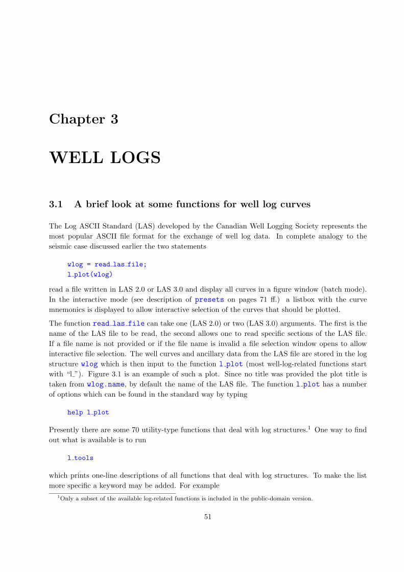
Chapter 3
WELL LOGS
3.1 A brief look at some functions for well log curves
The Log ASCII Standard (LAS) developed by the Canadian Well Logging Society represents the
most popular ASCII file format for the exchange of well log data. In complete analogy to the
seismic case discussed earlier the two statements
wlog = read las file;
l plot(wlog)
read a file written in LAS 2.0 or LAS 3.0 and display all curves in a figure window (batch mode).
In the interactive mode (see description of presets on pages 71 ff.) a listbox with the curve
mnemonics is displayed to allow interactive selection of the curves that should be plotted.
The function read las file can take one (LAS 2.0) or two (LAS 3.0) arguments. The first is the
name of the LAS file to be read, the second allows one to read specific sections of the LAS file.
If a file name is not provided or if the file name is invalid a file selection window opens to allow
interactive file selection. The well curves and ancillary data from the LAS file are stored in the log
structure wlog which is then input to the function l plot (most well-log-related functions start
with “l ”). Figure 3.1 is an example of such a plot. Since no title was provided the plot title is
taken from wlog.name, by default the name of the LAS file. The function l plot has a number
of options which can be found in the standard way by typing
help l plot
Presently there are some 70 utility-type functions that deal with log structures.1 One way to find
out what is available is to run
l tools
which prints one-line descriptions of all functions that deal with log structures. To make the list
more specific a keyword may be added. For example
1Only a subset of the available log-related functions is included in the public-domain version.
51
52 CHAPTER 3. WELL LOGS
0 0.2 0.42700
2800
2900
3000
3100
3200
3300
3400
3500
3600
3700
PRROCK
na
dept
h (m
)
0 50 100
CLAY
%
0 500010000
VSROCK
ft/s
0 50 100
SATNBRINE
%
0 50
PHI
%
0 1 2
x 104
VPROCK
ft/s
2000−12−25 (15:3:17)Manual_1
WELL #1
1 2 32700
2800
2900
3000
3100
3200
3300
3400
3500
3600
3700
RROCK
g/cm3
dept
h (m
)
Figure 3.1: Plot of all traces of log structure logout.
l tools las
lists not only those functions that deal with LAS files (the search is not case sensitive) but also
other functions that have the character group “las” as part of their description (the description of
l elastic impedance does not fit onto one line of this manual and, hence, as been broken into
two).
l elastic impedance Compute ‘‘elastic impedance’’ for user-defined
angles of incidence
read las file Read disk file in LAS 2.0 format
show las header Output/display header of LAS 2.0 file
write las file Write disk file in LAS 2.0 format
In a LAS file each log curve is associated with at least three pieces of information: a mnemonic,
units of measurement, and a description. Examples of mnemonics are “DT”, “DTCO”, or “BHC”
for sonic interval transit time, “RHOB” for bulk density, etc.; examples of units of measurement
are “us/ft” meaning µs/ft, or “g/cm3”, meaning g/cm3. Curve mnemonics are frequently chosen
to provide some idea of how the curve has been measured/computed and hence may vary from
one logging company or log analyst to the next. There is also a tremendous variation in the way
units are denoted. When writing a LAS file one commercial program, for example, denotes feet by
“F” which lead another commercial program, while converting non-metric units to MKS, to output
depth in Kelvin, as it obviously interpreted “F” as Fahrenheit.
3.1. A BRIEF LOOK AT SOME FUNCTIONS FOR WELL LOG CURVES 53
The function read las file leaves header mnemonics as they are in the LAS file (the only excep-
tion is “DEPT” which is converted to “DEPTH”). However, units of measurements are converted
to a standard form (for example, LAS file writers have come up with at least 6 different ways to
say “g/cm3”) — at least for those curves that are most relevant for someone dealing with seismic
data. Of course, misinterpretations are possible; however, “F” would be interpreted as “feet” and
converted to “ft” (and not assumed to represent Fahrenheit). This conversion is performed in
function unit substitution which contains the list of what is converted into what.
To simplify their use many functions assume standard mnemonics for curves. These standard
mnemonics are defined in function systemDefaults4Seislab in a global structure called CURVES.
They are shown in Tables 1-3 on pages 76 ff. Thus “acoustic impedance”, for example, has the
mnemonic aImp.
This list is likely to grow.
Several of the curves (those identifying lithology) are designated as logical. This means that their
values are either 1 (true) or 0 (false).
Obviously, curve mnemonics can be changed globally or locally at any time. The following code
fragment illustrates this.
well log = read las file;
well log = l rename(well log,{‘RHOB’,‘rho’},{‘DTCO’,‘DTp’}); 3a
well log = l seismic acoustic(well log);
It reads an LAS file with sonic and density curves, and changes their mnemonics of from “DTCO” to
“DTp” and from “RHOB” to “rho”, respectively. In the last statement the function, l seismic acoustic,
assumes that density and sonic curves use these standard mnemonics, computes compressional ve-
locity “Vp” and acoustic impedance “aImp” and adds them to the dataset well log.
One of the parameters set in the initialization function presets (see page 71 ff.) is
S4M.case sensitive. If this parameter is set to false, which is the default, then 3a could
have been written as
well log = l rename(well log,{‘rhob’,‘rho’},{‘dtco’,‘dtp’}); 3b
In fact any combination of upper-case letters and lower-case letters is permissible.
However, a user is not wedded to these standard mnemonics. First of all, they can be changed
in function systemDefaults4Seislab or by means of function l redefine. Assume it were
necessary to preserve the original mnemonics in the example above. Then one could write
well log = read las file;
l redefine({‘rho’,‘RHOB’},{‘DTp’,‘DTCO’});well log = l seismic acoustic(well log);
where l redefine changes the default mnemonics rho and DTp to RHOB and DT, respectively (note
that l redefine has no output argument; it changes fields of the global structure CURVES)
But the standard mnemonics can also be changed on a case-by-case basis. One could write
54 CHAPTER 3. WELL LOGS
well log = read las file;
well log = l seismic acoustic(well log,{‘rho’,‘RHOB’},{‘DTp’,‘DTCO’});
The two additional arguments tell l seismic acoustic that the density curve has mnemonic
RHOB (instead of the standard mnemonic rho) and the sonic log has mnemonic DTCO (instead of
the standard mnemonic DTp).
The two curves computed in l seismic acoustic in all the above cases would still have default
mnemonics Vp and aImp. But this could be changed as well. With either
well log = read las file;
l redefine({‘rho’,‘RHOB’},{‘DTp’,‘DTCO’},{‘Vp’,‘Vel’},{‘aImp’,‘IMP’});well log = l seismic acoustic(well log);
or
well log = read las file;
well log = l seismic acoustic(well log,{‘rho’,‘RHOB’},{‘DTp’,‘DTCO’}, ...
{‘aImp’,‘IMP’},{‘Vp’,‘Vel’});
the mnemonics of acoustic impedance and compressional velocity will be IMP and Vel, respec-
tively. In this last case,which avoids the call to function l redefine, the standard mnemonics
are not changed. Consequently, a subsequently called function that needs, for example, the acous-
tic impedance must be told explicitly what its mnemonic is. Thus the true benefit of standard
mnemonics accrues when a number of functions are to be executed in sequence: there is no need
to tell each of them what curve mnemonics to use. Renaming of curve mnemonics or redefin-
ing of standard curve mnemonics occurs only once — preferably right after reading the LAS file.
Thereafter, the code need not be changed if another log is to be processed in the same way.
3.2 Description of log structures
The log-related functions assume that a log is represented by a structure which — in addition to
the actual log curves represented by a matrix — contains necessary ancillary information in form of
the mnemonics associated with each curve, the units of measurement, and a more understandable
description. Furthermore, there can be parameters such as Kelly bushing elevation, water depth,
etc. Basically, a log structure has nine (ten if there are null values) required fields and any number
of optional fields. This description uses the variable ncurves to denote the number of curves in
the well log.
• type General identifier of the type of dataset. For a well log it is the string ‘well-log’.
• tag This field is used to identify the type of well log — if appropriate. The default tag is
‘unspecified’.
3.3. DESCRIPTION OF FUNCTIONS FOR WELL LOG ANALYSIS 55
• name Name associated with the dataset. This could be the well name. When read from a
LAS file it is the file name without .las extension. By default it is used as a plot title.
• first Start of log, (first depth value).
• last End of log, (last depth value).
• step Depth increment (0 if non-uniform).
• units Units of measurement for the depth.
• null No-data (null) value; generally NaN. This field is only present if there are null values.
In LAS files null values are frequently represented by the number -999.25.
• curves A matrix of log curves with ncurves columns; the first column must be DEPTH
and this description always refers to depth with the understanding that it could be something
equivalent such as TWT (two-way time).
• curve info Cell array of dimension ncurves×3. The first column contains the curve
mnemonics, the second column the units of measurement, and the last column a descrip-
tion of each curve. There must be one row for each curve. Obviously, the first row of
curve info pertains to the depth, and so curve info{1,2} must be the same as the field
units described above.
3.3 Description of functions for well log analysis
l check
Purpose: Check a log data structure for formal errors such as inconsistencies, missing required
fields, etc. It takes only one argument, the dataset to be checked. An example is
wlog=l data; l check(wlog)
which checks for errors of the structure wlog; if indeed errors are found, l check will print
messages explaining them. Otherwise, the message No formal errors found in ‘‘name’’(where name is the dataset name) will be printed.
It is expected that every log structure created or modified by a SeisLab function will pass this
consistency test; however, users may modify structures outside of these functions and, if these
changes are more severe, checking if they violate any formal requirements may be appropriate.
l compare
Purpose: Compare two or more log curves. The function plots one or more log curves from one
or more wells into one figure window. A simple example is
l compare({log1,‘Vp’},{log1,‘Vs’})
56 CHAPTER 3. WELL LOGS
which plots compressional velocity and shear velocity of log structure log1. Of course the curves
need not come from the same log structure.
l compare({log1,‘Vp’},{log2,‘Vp pred’})
compares a measured velocity curve of log1 with a predicted velocity curve from log2. If depth
units or units of measurement of the curves differ they are automatically converted to those of the
first log. There are a number of parameters that can be set. The following function call
l compare({log1,‘DT’,{‘color’,‘r’},{‘linewidth’,2},{‘legend’,‘Sonic log’}},...{log2,‘DTCO’,{‘color’,‘g’},{‘linewidth’,2},{‘legend’,‘Sonic log’}})
plots the first curve in red with a line width of 2 points and the second curve in green with the
same line width.
l convert
Purpose: Convert a matrix of curve values and three-column cell matrices with curve names,
curve units of measurement, curve description into a well log structure. An example is
wlog=l convert(columns,{‘depth’,‘ft’,‘Depth’; ...
’DTp’,‘us/ft’,‘Sonic’; ...
’VpVs’,‘n/a’,‘Vp-Vs ratio’; ...
’rho’,‘g/cm3’,‘Density’; ...
’epsilon’,‘n/a’,‘epsilon’; ...
’delta’,‘n/a’,‘delta’});
which converts the six-column matrix columns into a log structure with six curves with the
mnemonics depth, DTp, Vp, Vs, rho, epsilon, and delta. The first column of matrix
columns, representing the depth, must be strictly monotonic.
l crossplot
Purpose: Make cross-plots of log curves. A simple example, is
l crossplot(wlog,‘Vp’,‘rho’)
which creates a plot in which the horizontal axis is velocity and the vertical axis the density
(assuming curves Vp and rho are present in the log structure wlog). A plot like this could also
be generated with modest additional effort with standard MATLAB tools. The function is more
useful for more elaborate plots; an example is shown in Figure 3.2; it has been generated by
3.3. DESCRIPTION OF FUNCTIONS FOR WELL LOG ANALYSIS 57
04−Aug−2001 14:50:27Manual_crossplot
2000 2500 3000 3500 4000 4500 50002.1
2.15
2.2
2.25
2.3
2.35
2.4
2.45
2.5
2.55
2.6wlog_test
P−velocity (m/s)
Den
sity
(g/
cm3 )
ShaleSand
Figure 3.2: Cross-plot of velocity and density for two lithologies: sand (yellow diamonds) and shale
(gray dots); created by two calls to l crossplot
l crossplot(wlog test,‘Vp’,‘rho’,{‘depths’,3000,3500}, ...
{‘rows’,‘shale & rho > 2.1 & Vp < 5000’}, ...
{‘color’,[0.6, 0.6, 0.6]},{‘marker’,‘.’})l crossplot(wlog test,‘Vp’,‘rho’,{‘depths’,3000,3500}, ...
{‘rows’,‘sand & rho > 2.1 & Vp < 5000’}, ...
{‘color’,[1 0.8 0]},{‘marker’,‘d’},{‘figure’,‘old’})legend(‘Shale’,‘Sand’,4)
Here, log values are restricted to the depth range from 3000 to 3500 m, Furthermore, only depths
are considered for which the density is greater than 2.1 g/cm3 and the velocity is less than 5000
m/s. The first call to l crossplot displays the velocity-density relationship for shales, the second
the one for sands.
l curve math
Purpose: This function performs arithmetic using curves to append new curves or replace existing
ones. A curve is created through arithmetic operations on existing curves. A simple example is the
computation of the acoustic impedance from a sonic curve and a density curve. The resulting log
structure logout has all the curves of login and, in addition, an impedance curve.
logout = l curve math(login,‘add’,‘aImp=(1.0e6/DTp)*rho’,...
‘ft/sec x g/cm3’,‘Acoustic impedance’)
58 CHAPTER 3. WELL LOGS
The first argument is the input log, the second argument defines the operation to perform (add,
add ne, or replace) and the third is an expression in MATLAB syntax. A new curve with
mnemonic aImp is created by dividing 106 by the sonic log (creates velocity) and multiplying the
result by the density log. The last two arguments are the units and the description of the new
curve. In this example it is assumed that the original log has curves with mnemonics DTp and
rho representing a sonic and a density curve and that their units of measurement are µsec/ft and
g/cm3, respectively. The difference between add and add ne is that with the former the function
aborts with an error message if the mnemonic is already in use while it will overwrite it ( ne means
“no error”) in the latter case. On the other hand, replace will abort with an error message if the
curve to be replaced does not exist.
Another example is
logout = l curve math(login,‘replace’,‘depth=depth-login.ekb’,
‘m’,‘Depth below sea level’)
which changes the depth column (first curve) from measured depth to depth below sea level (ground
level) by removing the Kelly bushing elevation from the depth (assuming a parameter login.ekb
exists and depth and Kelly bushing elevation are measured in meter). If the first curve (depth) is
changed the fields first, step, and last of logout will reflect this change.
More sophisticated results can be achieved by repeated use of l curve math. The following two
lines of code create a curve of shale velocity with NaN’s wherever there is no shale.
wlog = l curve math(wlog,‘add’,‘Vp shale=Vp’,l gu(wlog,‘Vp’), ...
‘Compressional velocity in shale’)
wlog = l curve math(wlog,‘replace’,‘Vp shale(shale == 0) = NaN’)
The first line simply adds a copy of the velocity curve; the second function then places NaN’s in
this curve wherever the shale-curve is zero (the shale-curve is a curve which is 1 (true) when shale
is present and 0 (false) otherwise. Since the second function call replaces an existing curve the last
two arguments (units of measurements and description, respectively) can be omitted.
See also s select.
l histogram
Purpose: Create histogram(s) of values of a log curve. An example of the simplest use of this
command is
l histogram(wlog,‘rho’)
which plots a histogram of the density values (assuming that a density curve with mnemonic rho
exists in log structure log). A more sophisticated use is
l histogram(wlog,‘rho’,{‘litho’,‘shale’,‘w sand’,‘hc sand’})
3.3. DESCRIPTION OF FUNCTIONS FOR WELL LOG ANALYSIS 59
which creates a figure with three histograms — one for shale densities and one each for densities
of wet sand and hydrocarbon sand. With even more parameters
hstgrm = l histogram(wlog,‘rho’,{‘litho’,‘shale’,‘w sand’,‘hc sand’}, ...
{‘output type’,‘samples’},{‘edges’,2:0.1:2.8})
a user can specify that the y-axis of the histogram should be in samples (rather than percent (%),
the default), and specify the edges of the bins. Here the bin size is 0.1 g/cm3; the first bin starts
at 2.0 g/cm3, the last bin ends at 2.8 g/cm3. Furthermore, the function outputs a table structure
with the bin edges, the bin centers, and the histograms for shale wet sand, and hydrocarbon sand.
For this case the table structure looks like this:
title: ‘Histogram of well log’
edges: [2 2.1000 2.2000 2.3000 2.4000 2.5000 2.6000 2.7000 2.8000]
centers: [2.0500 2.1500 2.2500 2.3500 2.4500 2.5500 2.6500 2.7500]
column info: [1x1 struct]
rho4shale: [9x1 double]
rho4w sand: [9x1 double]
rho4hc sand: [9x1 double]
The field column info is a structure with the following fields:
edges: {‘g/cm3’ ‘Density’}centers: {‘g/cm3’ ‘Density’}
rho4shale: {‘Samples’ ‘Distribution of rho for shale’}rho4w sand: {‘Samples’ ‘Distribution of rho for wet sand’}
rho4hc sand: {‘Samples’ ‘Distribution of rho for hydrocarbon sand’}
l interpolate
Purpose: This function interpolates null values of all curves specified by an optional list of
mnemonics. The function assumes that null values are represented by NaN’s.
l lithocurves
Purpose: Create “logical” curves to identify lithology. The curve values are 1 (true) if the lithology
is present at a depth value and 0 (false) if it is not. It assumes that the input log has at least the
curves Vclay and computes the following additional curves if they do not exist (by default, the
function aborts with an error message if one of the lithologies to be created already exists; this
behavior can be changed via the keyword action)
sand sh sand shale
60 CHAPTER 3. WELL LOGS
based on the (default) condition
sand = vclay < 0.25
sh sand = vclay >= 0.25 & vclay <= 0.35
shale = vclay > 0.35
The cut-offs used above can be changed via keyword ‘clay cutoffs’.
If the input log has, in addition, the curve Sbrine the following additional logical curves are
computed (if they do not exist)
hc sand wet sand
Thus sand is split up into wet sand and hydrocarbon sand based on the (default) condition
hc sand = sand & sbrine <= 0.60
wet sand = sand & sbrine > 0.60
The water saturation cut-off can be changed via keyword ‘sw cutoff’. The above conditions
assume that the units of Vclay and Sbrine are fractions; they are appropriately modified if one or
both are in percent. Hence, if the default cut-offs are used and at least the Vclay curve is present
then all it takes is
wlog=l lithocurves(wlog)
It should be noted that the same end can be achieved, with somewhat more typing, via
wlog=l curve math(wlog,‘add’,‘sand=vclay < 0.25’,‘logical’,‘Sand’)
wlog=l curve math(wlog,‘add’,‘sh sand=vclay >= 0.25 & vclay < 0.35’, ...
‘logical’,‘Shaley sand’)
wlog=l curve math(wlog,‘add’,‘shale=vclay >= 0.35’,‘logical’,‘Shale’);
Splitting sand into wet and hydrocarbon sand would require two more calls to l curve math.
l lithoplot
Purpose: Plot log curves with colors and/or markers representing lithology. This requires that
‘logical’ curves representing lithology exist in the log structure. Such curves could, for example, be
created by means of function l lithocurves.
The simplest example is
l lithoplot(wlog)
which uses all the lithology curves in the log structure wlog to plot all the non-lithology curves.
In general, it is preferable to restrict the number of curves and the number of lithologies.
3.3. DESCRIPTION OF FUNCTIONS FOR WELL LOG ANALYSIS 61
l lithoplot(wlog,{‘curves’,‘Vp’,‘rho’,‘aImp’}, ...
{‘lithos’,‘shale’,‘sh sand’,‘wet sand’,‘gas sand’})
which only plots the P-velocity, density, and acoustic impedance with shale, shaley sand, wet sand,
and gas sand indicated by specific colors and markers. For a number of frequently used lithologies
these colors/markers are predefined (see help l lithoplot for specifics). Shale, for example is
represented by a gray dot (a small symbol because shale is generally quite dominant). It is, of
course possible to change all this. For example, the above example could be expanded to
l lithoplot(wlog,{‘curves’,‘Vp’,‘rho’,‘aImp’}, ...
{‘lithos’,‘shale’,‘sh sand’,‘wet sand’,‘gas sand’}, ...
{‘shale’,‘k’,‘.’},{‘sh sand’,[0.6, 0.6, 0.6],‘.’})
which redefines shales to be represented by black dots and shaley sands by gray dots. This example
also illustrates that colors represented by characters (‘r’ for red, ‘k’ for black, etc.) as well as
the RGB definition of colors can be used. An example of such a lithology plot is shown in Figure
3.3. It was created by
aux=l lithoplot(wlog2,{‘curves’,‘Vp’,‘rho’},{‘depths’,2000,2500}, ...
{‘lithos’,‘shale’,‘wet sand’,‘hc sand’})set(aux.axis handles(1),‘XDir’,‘reverse’)
Only log values that represent on of the three lithologies shale, wet sand, or hydrocarbon sand
are displayed. Log samples representing, say, shaley sand, limestone, or coal are not plotted.
The function l lithoplot has an optional output argument, the structure aux; it has a field
axis handles that is an array with the handles to all subplot axes. This is used here to reverse
the x-axis of the first subplot to make it conform to standard log-display practice.
l redefine
Purpose: Change one or more default (standard) curve mnemonics. The simplest form is
l redefine({‘rho’,‘rhob’})
which changes the default curve mnemonic for the bulk density from rho to rhob. This is an
alternative to changing the curve mnemonics in a log structure to be equal to the default mnemonics
(see l rename). An arbitrary number of default mnemonics can be changed with one l redefine.
l redefine({‘rhob’,‘rho’},{‘DT’,‘DTp’},{‘VCL’,‘Vclay’})
changes default curve mnemonics rho, DTp, Vclay to rhob, DT, Vcl, respectively.
This function changes the values of fields in global structure CURVES (see the description of presets
on pages 71 ff.)
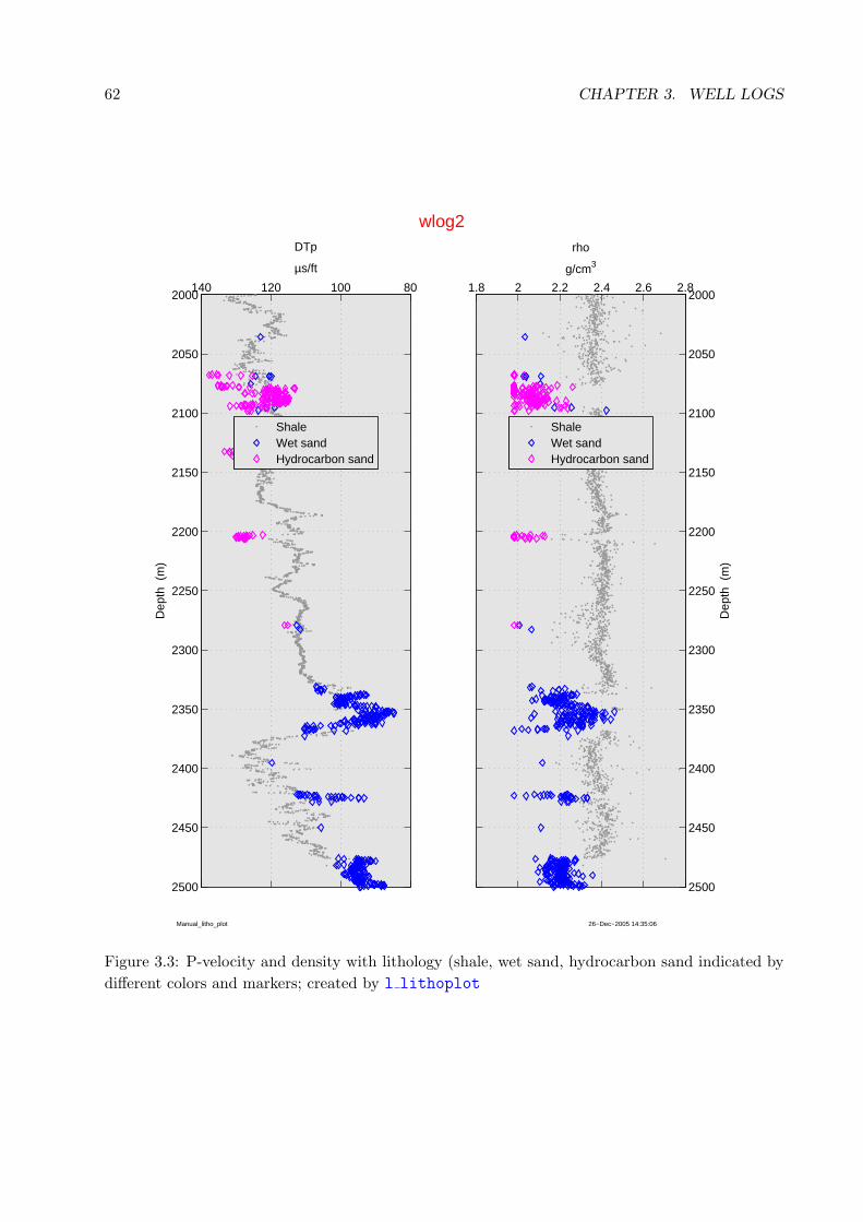
62 CHAPTER 3. WELL LOGS
26−Dec−2005 14:35:06Manual_litho_plot
wlog2
801001201402000
2050
2100
2150
2200
2250
2300
2350
2400
2450
2500
DTp
µs/ft
Dep
th (
m)
ShaleWet sandHydrocarbon sand
1.8 2 2.2 2.4 2.6 2.82000
2050
2100
2150
2200
2250
2300
2350
2400
2450
2500
rho
g/cm3
Dep
th (
m)
ShaleWet sandHydrocarbon sand
Figure 3.3: P-velocity and density with lithology (shale, wet sand, hydrocarbon sand indicated by
different colors and markers; created by l lithoplot
3.3. DESCRIPTION OF FUNCTIONS FOR WELL LOG ANALYSIS 63
l regression
Purpose: Compute attribute relationships between two or more log curves. A simple example of
its use is
wlog = l regression(wlog,‘vs=x1*vp+1000*x2’)
which computes parameters x1 and x2 so that the shear velocity vs is expressed “as well as
possible” in terms of a linear relationship with the compressional velocity vp. Vs (assuming that
curve mnemonics are not case-sensitive) and Vp must be curve mnemonics for shear velocity and
compressional velocity, respectively. The default meaning of the expression “as well as possible” is
(L1 norm)
|vs − x1vp + 1000x2| = min.
It is also possible to specify the L2 norm.
|vs − x1vp + 1000x2|2 = min).
by means of the keyword norm
wlog = l regression(wlog,‘vs=x1*vp+1000*x2’,{‘norm’,‘L2’})
l regression uses the MATLAB functions (Optimization Toolbox) fminunc (for unconstrained
minimization) and fmincon (for constrained optimization). These functions require a starting
value for each variable, and if none are provided as arguments (as in the example above) then
l regression sets the starting values of all parameters equal to 1.
In the relationship above the parameter x2 is multiplied by 1000. In theory, this is not necessary.
In practice, any parameter estimation program works best if the unknowns are balanced (for linear
systems this is equivalent to balancing matrix columns). The factor 1000 has been chosen to be in
the order of magnitude of compressional and shear velocities measured in m/s. Hence the default
starting value is not orders of magnitude off.
In general, it is good practice to use constraints to limit the search performed since regression
parameters could easily range from a compaction factor of the order of 10−4 m−1 to several thousand
ft/s as in the example above. It is even helpful to tell l regression if one or more parameters
must be non-negative. Bounds on the parameter values are particularly important if parameters
are exponents or part of exponential functions.
In the example above all depth levels in the log structure are used for which there are valid
compressional AND shear velocities. It is possible to restrict these values to a range of depth
and/or use logical constraints. For example
wlog = l regression(wlog,‘vs=x1*vp+1000*x2’,{‘depths’,2000,3000}, ...
{‘rows’,‘sand’})
restricts the samples to sands (for which the values of logical curve sand are equal to 1) in the
depth range from 2000 to 3000 m (assuming the depth units are m). Of course, a logical curve with
64 CHAPTER 3. WELL LOGS
mnemonic sand must exist in the log structure wlog (see function l lithocurves). The keywords
rows and depths are those used in l select to extract specific rows from a log structure. The
above statement could also have been written as
wlog = l regression(wlog,‘vs=x1*vp+1000*x2’, ...
{‘rows’,‘sand & depth >= 2000 & depth <= 3000’})
The expression relating shear velocity and compressional velocity used above is linear. It does
not have to be. Any valid MATLAB statement is allowed provided the only variables are curve
mnemonics and up to 9 parameters (x1, x2, ...., x9) and there is only one variable (mnemonic
of an existing curve) to the left of the equal sign. The parameters can be constrained by specifying
lower and upper bounds. For example
wlog = l regression(wlog,‘vs=x1*vp+1000*x2’,{‘lbounds’,0,-inf})
requires that x1 is non-negative since it has a lower bound 0; x2 is not constrained since its lower
bound is −∞. The keyword ubounds can be used to set upper bounds. If bounds are given they
must be given for all parameters, but inf and -inf are allowed. If bounds are known they should
be given to prevent the algorithm from going astray.
As mentioned before fitting can be done via either the L1-norm or the L2-norm. However, there
is a third option. It is based on the L1-norm but treats positive deviations different from negative
deviations. With, say,
g(x1, x2) = vs − x1vp − 1000x2;
it can be expressed as
f1H(g(x1, x2)) ∗ g(x1, x2)− f2H(−g(x1, x2))g(x1, x2) = min. (3.1)
where H(·) is the Heaviside function
H(x) =
{1 for x > 0
0 for x < 0
and f1 and f2 are positive factors. Obviously, expression (3.1) is equivalent to f1|g(x1, x2)| if
f1 = f2. However, if f1 < f2, then positive deviations receive lower weight than negative ones. The
regression will tend to better match the large values. If f1 > f2, the result is the opposite. Figure
3.4, which is the result of the following MATLAB statements illustrates this.
expression = ‘rho=x1*(depth/1000)ˆx2’;
[log curves,aux1] = l regression(log curves,expression, ...
{‘norm’,‘L1’},{‘lbounds’,0,0},{‘mnem’,‘L1 fit’}, ...
{‘description’,‘L1 fit to density’});[log curves,aux2] = l regression(log curves,expression, ...
{‘norm’,‘L2’},{‘lbounds’,0,0},{‘mnem’,‘L2 fit’}, ...
{‘description’,‘L2 fit to density’});
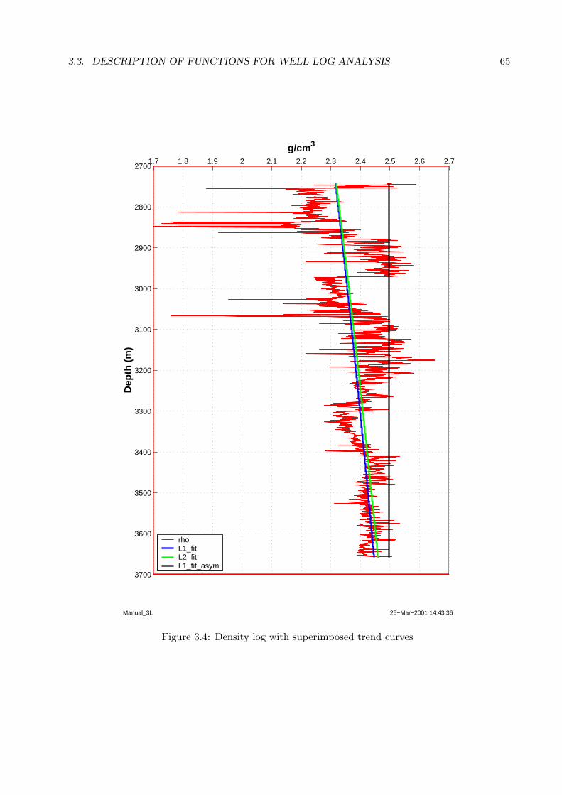
3.3. DESCRIPTION OF FUNCTIONS FOR WELL LOG ANALYSIS 65
25−Mar−2001 14:43:36Manual_3L
1.7 1.8 1.9 2 2.1 2.2 2.3 2.4 2.5 2.6 2.72700
2800
2900
3000
3100
3200
3300
3400
3500
3600
3700
g/cm3
Dep
th (
m)
rhoL1_fitL2_fitL1_fit_asym
Figure 3.4: Density log with superimposed trend curves
66 CHAPTER 3. WELL LOGS
[log curves,aux3] = l regression(log curves,expression, ...
{‘norm’,‘L1’,0.1,1},{‘lbounds’,0,0},{‘mnem’,‘L1 fit asym’}, ...
{‘description’,‘L1 asymm. fit to density’});l compare({log curves,‘rho’},{log curves,‘L1 fit’,{‘linewidth’,2}}, ...
{log curves,‘L2 fit’,{‘linewidth’,2}}, ...
{log curves,‘L1 fit asym’,{‘linewidth’,2}}, ...
{‘parameters’,{‘lloc’,3}})
L1-norm and L2-norm fits are close together with the latter slightly higher, and the asymmetric fit
is clearly separated from the two.
l rename
Purpose: Change one or more curve mnemonics. The simplest form is
log = l rename(log,{‘rhob’,‘rho’})
which changes the mnemonic RHOB of a density curve (assuming curve mnemonics have been defined
as not case-sensitive; see function presets) to rho, the standard density mnemonic used in SeisLab.
The above statement is equivalent to
log = l curve(log,‘rename’,‘rhob’,‘rho’)
In both statements units of measurement and curve description are not changed. The main differ-
ence between l rename and l curve with the ‘rename’ option is that the former allows renaming
of more than one curve. Thus,
log new = l rename(log,{‘rhob’,‘rho’},{‘dtco’,‘DTp’},{‘VCL’,‘Vclay’})
renames the three curves with mnemonics RHOB, DTCO, and VCL to the standard SeisLab mnemon-
ics. Curve mnemonics are renamed in the order they are listed. Hence,
log new = l rename(log,{‘rho’,‘rho1’},{‘rhob’,‘rho’})
first changes rho to rho1 and then changes rhob to rho.
The function aborts with an error message if a new curve mnemonic is already in use.
A related function is l redefine which changes/redefines one or more default (standard) curve
mnemonics. This is an alternative to changing the curve mnemonics in a log to equal the default
mnemonics.
l resample
Purpose: This function re-samples the curves of a log to a new, uniform sample interval. This
sample interval can be smaller or larger than the original sample interval of the input data.
3.3. DESCRIPTION OF FUNCTIONS FOR WELL LOG ANALYSIS 67
l select
Purpose: Select a subset of log curve(s) and/or depth values from a log structure.
A simple example is
new log = s select(wlog,{‘curves’,‘DTp’,‘rho’,‘shale’})
which copies three curves (compressional sonic, density, and a logical curve which is true when a
sample represents shale and false if not) to a new log structure, new log. The function terminates
abnormally with an error message if any one of the three curves is not present in wlog. Of course,
one can also chose a depth range. The following function call is identical to the one above, except
that the three curves in new log are restricted to depths ranging from 3000 to 4000 (the units are
the those used for the depth).
new log=s select(wlog,{‘curves’,‘DTp’,‘rho’,‘shale’},{‘depths’,3000,4000})
There is a third way in which data from a log structure can be selected; the following line of code
shows an example.
new log = s select(wlog,{‘rows’,‘shale == 1’})
In this case new log includes all curves of wlog but only for those depths for which the shale
marker is equal to 1 (i.e. the log curves only for shale).
l plot
Purpose: This function plots log curves. Using all the default settings
l plot(wlog)
plots all the curves in the log structure wlog, each with its own axes. For fewer than 5 curves
the default figure orientation is “portrait”, otherwise it is “landscape”. The string in field name is
plotted as title. An example of the output is shown in Figure 3.1. For log structures with a large
number of curves is it may be more practical to restrict the number of curves plotted. An example
is
l plot(slog,{‘curves’,‘dtp’,‘dts’},{‘depths’,2000,3000})
which not only restricts the number of curves plotted to compressional and shear velocity but also
the range of depths (from 2000 to 3000 in whatever depth units the log structure uses). Other
keywords that can be used are ‘figure’ (to specify if a new figure should be created (default) or
if an existing figure should be used), ‘orient’ to specify figure orientation if the default described
above is not appropriate, and ‘color’ to assign a curve color (default is red); all curves are plotted
68 CHAPTER 3. WELL LOGS
in the same color. Right-clicking a curve brings up a menu that allows one to change curve color,
line style, line thickness, etc.
If one of the curve mnemonics requested via keyword ‘curves’ does not exist in the log structure
a warning message is issued and the corresponding subplot window is left empty.
l plot1
Purpose: Like l plot this function plots log curves. However, all log curves are plotted in one
and the same window. If the units of measurement of all plotted curves are the same they are used
to annotate the horizontal axis. If this is not the case, the horizontal axis ia annotated from 0 to
1, and all curves are scaled and shifted in such a way that the smallest value is 0 and the largest
value is 1. The true minimum and maximum values are plotted as part of the legend next to the
curve mnemonic. l plot1 understands all the keywords used by l plot (with the exception that
the plural ‘colors’ is used instead of the singular in l plot). Hence the example above reads
l plot1(slog,{‘curves’,‘dtp’,‘dts’},{‘depths’,2000,3000})
The number of curves plotted cannot exceed the number of colors available. Since there are 7 colors
preset, a maximum of 7 curves can be plotted without increasing the number of colors. If there are
more curves to plot than there are colors available, curves for which there are no colors left will not
be plotted and an alert message will be printed.
Additional keywords, not available in l plot, are ‘linewidth’ and ‘lloc’; they set the line
width of the curves and the location of the legend.
l tools
Purpose: This function writes one-line description for log function (in alphabetic order). The
simplest call is l tools which displays this description for all log functions. The output can be
restricted by adding a search string. For example, l tools create will show all functions that
create log datasets; l tools las will show all functions that deal with LAS files. The search is
not case-sensitive.
l trim
Purpose: This function removes leading and trailing rows from log curves if they contain null
values. Null values bracketed by non-null values are retained. The function assumes that null
values are represented by NaN’s. If this is not the case they are replaced by NaN’s in the output
structure. With the minimum number of input arguments
wlog=l trim(wlog);
3.3. DESCRIPTION OF FUNCTIONS FOR WELL LOG ANALYSIS 69
the function l trim removes leading and/or trailing null values that are common to ALL curves
with the exception of the depth (first column of the curve matrix) which must not have null values
at all. This is equivalent to
wlog=l trim(wlog,‘all’);
This is a very benign operation as it does not remove any valid data. Of a more drastic nature is
this function with the option ‘any’
wlog=l trim(wlog,‘any’);
which removes leading and/or trailing rows of the matrix of curve values if ANY of the curves
contains a null value. Of course, if one of the curves is very short (say a particular log had been
measured only over a reservoir interval) all other curves are shortened to this interval as well. To
avoid problems with such short curves it is possible to restrict the number of curves for which the
condition is evaluated. For example,
wlog=l trim(wlog,‘any’,{‘DTp’,‘rho’});
removes leading and/or trailing rows of the matrix of curve values if the sonic and/or the density
log have null values. All other curves are disregarded.
As mentioned above, gaps, i. e. null values within log curves (null values preceded and followed
by valid curve values), are likely to be retained. The function l interpolate can be used to
interpolate across such gaps. The function l curve can be used to find out if any of the log curves
have gaps.
read las file
Purpose: This function reads a disk file written in LAS format and outputs a log structure. The
function tries to be lenient and accept files even if they do not quite follow the LAS standard.
show las header
Purpose: This function reads a disk file written in LAS format and outputs the header to a file
or prints it to the screen.
write las file
Purpose: This function writes a log structure to disk in LAS format.

70 CHAPTER 3. WELL LOGS
Chapter 4
GENERAL TOPICS
4.1 Initialization Function
presets
Purpose: This function calls two other functions, systemDefaults4Seislab and userDefaults4Seislab.
The former, called first, creates four global structures, CURVES, CURVE TYPES, TABLES, and S4M,
which are used by many SeisLab functions. The last of them, S4M, is of particular importance; some
fields of this structure are intended to be customized by a user. These fields should be redefined
in function userDefaults4Seislab. In fact, any field set in systemDefaults4Seislab can be
overridden in userDefaults4Seislab — or anywhere else for this matter.
One can use the commands
presets
global S4M
show(S4M)
to display the alphabetically sorted fields of S4M.
Some of the key fields of S4M with their default settings are:
• seismic path — path to the directory with seismic data. SEG-Y files are assumed to have
the file extension “sgy” or “segy”. If a file name is not specified when read segy file or
write segy file is called a file selection window opens. The directory in which it starts is
set by this variable. This may save a number of mouse clicks. Analogous fields exist for log
data (usually extension ”las”), mat files (extension ”mat”), and table files (extension ”tbl”).
• default path — This is a global variable with a path for files with file extensions other
than ‘‘sgy’’, ‘‘segy’’, ‘‘las’’, ‘‘tbl’’, or ‘‘mat’’.
Those defined in systemDefaults4Seislab are:
71
72 CHAPTER 4. GENERAL TOPICS
• script
Default is ‘’; but if the initialization function presets is called from a script this field stores
the name of that script.
• alert = true
This parameter specifies if, in certain circumstances, messages should be printed to alert the
user to certain situations or results.
• case sensitive = false
This parameter specifies whether or not seismic header mnemonics and curve mnemonics of
well logs are case-sensitive; i.e. it establishes if ‘CDP’ is the same trace header as ‘cdp’ or
if ‘RHOB’ is the same curve mnemonic as ‘rhob’ or ‘Rhob’ (with the default setting they
are).
• deployed = false
This parameter specifies if one is running a compiled version of SeisLab (compiled versions
of Matlab functions may be somewhat restricted in their functionality; this limitation went
away with Matlab versions 7.x).
• experience=1
Experience level of a user. Three values are supported: Novice: -1; User: 0; Expert: 1.
Mostly used in compiled versions of SeisLab.
• figure labels = true
Add a text label, S4M.plot label, in the lower left corner of a plot and date/time, S4M.time,
in the lower right corner. They are not plotted if this field id set to false.
• font name = ‘Arial’
Name of default font for plots.
• fp format = ‘ieee’
Floating point format used when writing data to a SEG-Y file. Default is IEEE with big-
endian byte ordering which is now part of the SEG-Y standard.
• history = true
The default setting of this field is 1 (true). This means that seismic datasets have a field
history. Each seismic function adds one line to the history field before it outputs the
seismic data. This way every seismic dataset has a kind of processing history attached.
Seismic functions add information to the history field of any dataset they process (unless
they are too deep down in the calling sequence; this is to avoid cluttering the history field).
• history level = 1
Specifies how deep in the calling sequence a function must be so that it does not write to the
history field even if S4M.history == 1.
• interactive=false
If interactive is off (false) a running script or function will not stop with an interactive mes-
sage to request a user action but will perform the default action. An example is l plot(wlog)
4.1. INITIALIZATION FUNCTION 73
which plots the curves of well log wlog. If interactive=true and if no curves have been
specified in the argument list a listbox requesting selection of the curves to plot will pop up;
however, if interactive=false then l plot will plot all the curves without asking the
user.
• mymatlab=fileparts(which(’presets’))
Name of the folder with a user’s Matlab files (actually the folder in which function presets
is).
• name=’SeisLab’
Name of the package; used in the title pane of figures
• ntr wiggle2color=101
Number of traces for which automatic seismic plotting (e.g. s plot, s ispectrum) switches
from wiggle trace to color (s wplot always plots wiggles and s cplot always makes color
plots).
• plot label
Label for lower left corner of plots; default is S4M.script.
• plot labels on
This parameter specifies if there should be labels at the bottom of a figure (a label in the
lower left corner (see plot label) and the date and time in the lower right corner). Possible
values are true and false. Default: true.
• eps directory=fullfile(’C:\Documents and Settings’, ...
getenv(’USERNAME’),‘My Documents’,‘My Pictures’)
Directory used to store encapsulated PostScript files. These files are intended for use in
LATEXdocuments. They are created by clicking the ”Save plot” figure-menu button and se-
lecting the “EPS” option.
• pp directory=fullfile(’C:\Documents and Settings’, ...
getenv(’USERNAME’),‘My Documents’,‘My Pictures’)
Directory used to store PowerPoint files. These files use the EMF (Enhanced Meta File)
format which converts readily to Microsoft Office drawing objects and can then be edited.
They are created by clicking the ”Save plot” figure-menu button and selecting the “EMF”
option.
• start time
Set to date and time when presets was run.
Executing presets at the beginning of a script is a good idea because it restores the de-
fault values of all global parameters and updates the time information in S4M.start time.
Several plot programs put this time in the lower right corner of the plot. This way all plots
generated with the same script during the same run bear the same “time stamp”; see also
S4M.plot labels on.
• matlab version = 7.1
Version of Matlab (the value 7.1 is just an example). Determined by examining the output of
74 CHAPTER 4. GENERAL TOPICS
Matlab’s version command. This parameter is used in some functions that require different
code depending on the version of Matlab used.
• landscape
Default figure position and size of landscape plots on the screen.
• portrait
Default figure position and size of portrait plots on the screen.
• seismic path — path to the directory with seismic data. If a file name is not specified
when read segy file or write segy file is called a file selector window opens. The
directory in which it starts is set by this variable. This may save a number of mouse clicks.
Analogous fields exist for log data (extension ”log”), mat files (extension ”mat”), and table
files (extension ”tbl”).
• log path — path to the directory with well data. If a file name is not specified when
read las file or write las file is called a file selector window opens. The directory
in which it starts is set by this variable.
• default path — This is a global variable with a path for files with file extensions other
than ‘‘sgy’’, ‘‘las’’, ‘‘tbl’’, or ‘‘mat’’.
The file presets calls functions systemDefaults4Seislab and userDefaults4Seislab (if it
exists). The latter is meant to be customized by the user. Function presets should be called prior
to using any of the SeisLab functions.
Hence the first lines of a script might look like this:
clear all
presets
Others global variables are more general and are set in function systemDefaults4Seislab which
is called by presets.
• CURVES — defines default curve mnemonics for log structures (see Tables 4.2, 4.1, and 4.3)
• CURVE TYPES — defines types of curves (e.g. impedance) of interest for geophysical work..
This is a five-column cell array.
1. type of curve (curve name)
2. possible units of measurements separated by a vertical bar (“|”). Units of measurements
are used for a tentative determination of the curve type (there are obviously different
curves that have the same mnemonics (e.g. clay volume and water saturation or P-
velocity and S-velocity).
3. Mnemonics for curve types; these mnemonics are largely identical with the corresponding
curve mnemonics (see global variable CURVES)
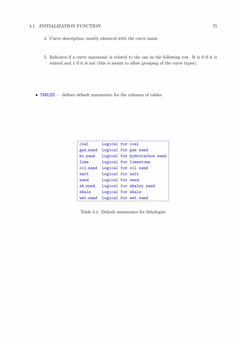
4.1. INITIALIZATION FUNCTION 75
4. Curve description; mostly identical with the curve name
5. Indicator if a curve mnemonic is related to the one in the following row. It is 0 if it is
related and 1 if it is not (this is meant to allow grouping of the curve types).
• TABLES — defines default mnemonics for the columns of tables.
coal Logical for coal
gas sand Logical for gas sand
hc sand Logical for hydrocarbon sand
lime Logical for limestone
oil sand Logical for oil sand
salt Logical for salt
sand Logical for sand
sh sand Logical for shaley sand
shale Logical for shale
wet sand Logical for wet sand
Table 4.1: Default mnemonics for lithologies
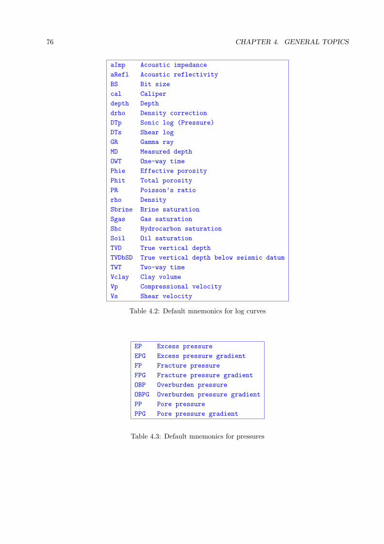
76 CHAPTER 4. GENERAL TOPICS
aImp Acoustic impedance
aRefl Acoustic reflectivity
BS Bit size
cal Caliper
depth Depth
drho Density correction
DTp Sonic log (Pressure)
DTs Shear log
GR Gamma ray
MD Measured depth
OWT One-way time
Phie Effective porosity
Phit Total porosity
PR Poisson’s ratio
rho Density
Sbrine Brine saturation
Sgas Gas saturation
Shc Hydrocarbon saturation
Soil Oil saturation
TVD True vertical depth
TVDbSD True vertical depth below seismic datum
TWT Two-way time
Vclay Clay volume
Vp Compressional velocity
Vs Shear velocity
Table 4.2: Default mnemonics for log curves
EP Excess pressure
EPG Excess pressure gradient
FP Fracture pressure
FPG Fracture pressure gradient
OBP Overburden pressure
OBPG Overburden pressure gradient
PP Pore pressure
PPG Pore pressure gradient
Table 4.3: Default mnemonics for pressures
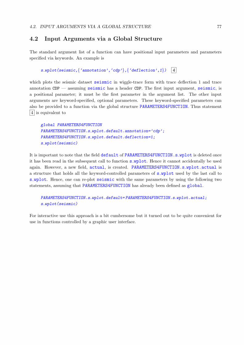
4.2. INPUT ARGUMENTS VIA A GLOBAL STRUCTURE 77
4.2 Input Arguments via a Global Structure
The standard argument list of a function can have positional input parameters and parameters
specified via keywords. An example is
s wplot(seismic,{‘annotation’,‘cdp’},{‘deflection’,1}) 4
which plots the seismic dataset seismic in wiggle-trace form with trace deflection 1 and trace
annotation CDP — assuming seismic has a header CDP. The first input argument, seismic, is
a positional parameter; it must be the first parameter in the argument list. The other input
arguments are keyword-specified, optional parameters. These keyword-specified parameters can
also be provided to a function via the global structure PARAMETERS4FUNCTION. Thus statement
4 is equivalent to
global PARAMETERS4FUNCTION
PARAMETERS4FUNCTION.s wplot.default.annotation=’cdp’;
PARAMETERS4FUNCTION.s wplot.default.deflection=1;
s wplot(seismic)
It is important to note that the field default of PARAMETERS4FUNCTION.s wplot is deleted once
it has been read in the subsequent call to function s wplot. Hence it cannot accidentally be used
again. However, a new field, actual, is created. PARAMETERS4FUNCTION.s wplot.actual is
a structure that holds all the keyword-controlled parameters of s wplot used by the last call to
s wplot. Hence, one can re-plot seismic with the same parameters by using the following two
statements, assuming that PARAMETERS4FUNCTION has already been defined as global.
PARAMETERS4FUNCTION.s wplot.default= PARAMETERS4FUNCTION.s wplot.actual;
s wplot(seismic)
For interactive use this approach is a bit cumbersome but it turned out to be quite convenient for
use in functions controlled by a graphic user interface.
Index
absorption filters, 40
alert, 72
arguments, see input arguments
case-sensitive, 53
command-line help, 3
cursor tracking, 27
CURVE TYPES, see global variables
CURVES, see global variables
EPS files, 73
example files
Examples4LogOnSeismicPlot, 47, 48
Seismic examples1, 40, 47
Seismic examples2, 40
Seismic log examples1, 49
Seismic phase rotation, 36
Seismic principal components, 43
figure labels, 6
functions related to pseudo-wells
pw tools, 3
function overloading, 20–22
general functions
presets, 2, 10, 14, 16, 22, 53, 61, 66, 71–74
show precision, 21, 22
systemDefaults4Seislab, 2, 53, 71, 74
timeStamp, 14
userDefaults4Seislab, 2, 71, 74
global variables
CURVES, 53, 61, 71
CURVE TYPES, 71, 74
PARAMETERS4FUNCTION, 77
S4M, iii, 4–6, 14, 18, 22, 24, 30, 34, 71, 73, 74
TABLES, 71
headers, 13–14, 16–18, 23, 26, 37
help, see command-line help
history, 72
impedance
acoustic, 53, 54
elastic, 52
implied header, see pseudo-header
initialization, see general functions: presets, 2
input arguments, 3–4
via global variable, 77
keyword abbreviation, 4
LAS file, 51–54
menu
Modify display, 30
Options, 27
Save plot, 27
Save plot, 6
mnemonics
case-sensitive, 24, 53
curve, 53
standard for curves, 53, 54
operator overloading, 18–20
overloading, see operator overloading or function
overloading
parameter abbreviation, see keyword abbrevia-
tion
PARAMETERS4FUNCTION, see global variables
plotting
log curves, 67
seismic data, 29
seismic data, 27–34
PowerPoint files, 73
precision, 5–6
78
INDEX 79
principal components, 42, 44
pseudo-header, 16, 23, 27, 41, 46
Q-filter, see absorption filter
required fields
seismic data set, 15
well log, 54
S4M, see global variables
sample data, see test data
Save plot menu, 27, 73
scroll bars, 27
SEG-Y file, 26
SEG-Y file, 12, 13, 15–18, 23, 25, 26, 48, 72
seismic headers, see headers
seismic functions
s wavelet4hampson russell, 26
S4M, 31
double, 5
ds gh, 14
ds header sort, 42
presets, 6, 34
read segy file, 9, 10, 17, 22–25, 74
s append, 37, 45
s attributes, 37
s check, 38
s compare, 11, 31
s convert, 38
s cplot, 30, 31, 73
s create qfilter, 40
s create wavelet, 19, 40
s data3d, 4
s data, 4
s filter, 11
s gd, 14
s gu, 14
s header math, 41
s header plot, 13, 32
s header sort, 45
s hesader, 40
s history, 42
s ispectrum, 34, 35, 73
s phase rotation, 44
s plot, 9, 27, 29, 31, 73
s principal components, 42
s rm zeros, 25
s seismic4jason, 26
s select, 22, 42, 46, 47
s shift, 45, 47
s slice3d, 32
s spectrum, 32
s stack, 47
s tools, 3, 11, 12, 36, 48
s wavelet4landmark, 26
s wavelet from hampson russell, 26
s wavelet from landmark, 26
s wavextra, 42, 48, 49
s wiener filter, 49
s wplot, 4, 7, 10, 31, 42, 73, 77
show precision, 21, 22
single, 5
userDefaults4Seislab, 6
write segy file, 74
seismic data
input/output, 22–26
comparing, 11, 31
display, 27–34
plotting, 10, 27–34
reading, 9
table-related functions
t tools, 3
TABLES, see global variables
test data, 4
three-dimensional data, 24, 25, 32
time stamp, 73
unit substitution, 53
wavelet estimation, 48
well log functions
l curve, 66
l elastic impedance, 52
l lithocurves, 64
l lithoplot, 60–62
l plot1, 68
l plot, 51, 67, 72, 73

80 INDEX
l redefine, 53, 54, 61
l rename, 53, 66
l seismic acoustic, 53, 54
l tools, 3, 68
l trim, 68, 69
read las file, 51, 53, 54, 69, 74
show precision, 21, 22
unit substitution, 53
write las file, 74
Wiener filter, 49
workflow, 7