sedimentgenerated noise and bed stress in a tidal...

JOURNAL OF GEOPHYSICAL RESEARCH: OCEANS, VOL. 118, 1–17, doi:10.1002/jgrc.20169, 2013

Sediment-generated noise and bed stress in a tidal channelChristopher Bassett,1 Jim Thomson,2 and Brian Polagye1

Received 24 October 2012; revised 13 March 2013; accepted 20 March 2013.

[1] Tidally driven currents and bed stresses can result in noise generated by movingsediments. At a site in Admiralty Inlet, Puget Sound, Washington State (USA), peak bedstresses exceed 20 Pa. Significant increases in noise levels are attributed to mobilizedsediments at frequencies from 4–30 kHz with more modest increases noted from1–4 kHz. Sediment-generated noise during strong currents masks background noise fromother sources, including vessel traffic. Inversions of the acoustic spectra for equivalentgrain sizes are consistent with qualitative data of the seabed composition. Bed stresscalculations using log layer, Reynolds stress, and inertial dissipation techniques generallyagree well and are used to estimate the shear stresses at which noise levels increase fordifferent grain sizes. Regressions of the acoustic intensity versus near-bed hydrodynamicpower demonstrate that noise levels are highly predictable above a critical thresholddespite the scatter introduced by the localized nature of mobilization events.Citation: Bassett, C., J. Thomson, and B. Polagye (2013), Sediment-generated noise and bed stress in a tidal channel, J. Geophys.Res. Oceans, 118, doi:10.1002/jgrc.20169.

1. Introduction[2] Sources of ambient noise in the ocean have been

the focus of numerous scientific studies dating back toWorld War II. Among the most commonly identifiedsources of ambient noise are shipping traffic [Wenz, 1962;Greene and Moore, 1995], weather [Wenz, 1962; Nystuenand Selsor, 1997; Ma et al., 2005], biological sources[Greene and Moore, 1995], and molecular agitation [Mellen,1952]. A more limited body of research identifies themotion of different sized sediment grains due to strongcurrents or surface waves as an ambient noise source[Voglis and Cook, 1970; Harden Jones and Mitson, 1982;Thorne, 1986b; Thorne et al., 1989; Thorne, 1990; Masonet al., 2007]. Noise generated by mobilized sediments isreferred to as sediment-generated noise. The frequency ofsound produced by particle collisions can be related to thesize of the mobile particles [Thorne, 1986a]. Given thatincipient motion of particles is driven by hydrodynamic con-ditions, for water depths on the order of 100 m, noise fromcoarse-grained sediments is only likely to be produced byhigh-current environments (e.g., current velocities >2 m s–1),restricting the geographic range in which this sound makesa significant contribution to ambient noise levels. In shal-lower water (i.e., depths on the order of 10 m or less), noise

Additional supporting information may be found in the online versionof this article.

1Department of Mechanical Engineering, University of Washington,Seattle, Washington, USA.

2Applied Physics Laboratory, University of Washington, Seattle,Washington, USA.

Corresponding author: C. Bassett, Department of Mechanical Engineer-ing, University of Washington, Stevens Way, Box 352600, Seattle, WA98103, USA. ([email protected])

©2013. American Geophysical Union. All Rights Reserved.2169-9275/13/10.1002/jgrc.20169

from the resuspension and transport of sediments by surfacewaves and wave-current interactions is also possible andmore likely to be observed over a broader geographic range.

[3] A lack of data identifying sediment-generated noiseas an important ambient noise source in a range of coastalenvironments represents a data gap with implications forpassive acoustic studies of marine species that inhabit suchareas (i.e., SNR for detection, classification, and localiza-tion algorithms), and for monitoring anthropogenic noise inthese areas. For example, tidal energy projects are in variousstages of development in coastal waters of the United States,Canada, the United Kingdom, Ireland, and South Korea.There are significant knowledge gaps with respect to possi-ble environmental impacts of tidal energy projects [Polagyeet al., 2011]. Sites suitable for tidal energy experience strongcurrents (>2 m s–1) that, depending on bottom type, couldmobilize sediments. Sediment-generated noise needs to beunderstood to design effective characterization and monitor-ing studies of the sound produced by tidal energy projectsand its effects on marine mammals.

[4] The conditions under which incipient motion of par-ticles occurs has long been an active research area. Shields’[1936] commonly cited work noted that lack of similar-ity between experiments and a lack of understanding ofnatural processes affecting motion of the bed were thetwo most important difficulties faced in developing rela-tionships between hydrodynamic conditions and bed loadtransport. To address these problems, controlled laboratoryexperiments were performed on bed types consisting ofhomogenous grain sizes with different densities. Resultswere presented in terms of dimensionless parameters to gen-eralize the results. The non-dimensionalized tractive forces,called the Shields parameter (‚b), were described as

‚b =�b

(�s – �)gD, (1)

1

BASSETT ET AL.: SEDIMENT-GENERATED NOISE

where �b is the bed stress, �s is the density of the sediment,� is the density of the water, g is gravity, and D is the diam-eter of the sediment grain. Results were presented againstthe grain Reynolds number (Re�) using the shear velocity(u�) as the characteristic velocity scale. For a particular flowregime (i.e., Re�), once the Shields parameter exceeded acritical value, incipient motion occurred. The empirical rela-tionships identified by Shields have been revisited numeroustimes in the literature. For example, Miller et al. [1977]and the references therein include relationships for incipientmotion of coarse-grained sediments. Miller et al. noted thatpredictions of incipient motion are difficult in complex nat-ural environments due to turbulence, bed forms, and grainsize distributions.

[5] Incipient motion of particles is often presented asa function of the mean shear stress or shear velocity.Field data [Heathershaw and Thorne, 1985], experimentalresults [Diplas et al., 2008], and numerical analysis [Lee andBalachandar, 2012] have highlighted how drag forces andturbulence can affect critical shear stresses. Unlike Shields[1936], these studies suggest that drag forces on individualgrains, rather than overall bed stresses, are more appropriatefor predicting incipient motion. Instantaneous forces asso-ciated with turbulent fluctuations can mobilize grains, evenwhen mean shear stresses are below critical values. Instan-taneous near-bed forces are, however, difficult to quantify inhigh-energy field environments.

[6] Once sediments are mobilized, there are two mecha-nisms by which sound is generated: bed load and saltation[Mason et al., 2007]. Bed load is the sustained motion ofparticles as a result of intergranular forcing and saltation isthe partial entrainment and resettlement of grains that aretoo large for sustained motion across the seabed. Regard-less of the type of motion, sound is generated as a result ofcollisions between individual particles.

[7] Laboratory experiments using artificial and real sed-iments have demonstrated that the spectral structure ofsediment-generated noise is related to the material propertiesand size of the particles by

fr � 0.182�

E�(1 – �2)

�0.4 � g0.1

D0.9

�, (2)

where fr is the resonant frequency, E is Young’s modu-lus, � is Poisson’s ratio, � is the particle density, g isthe gravitational acceleration, and D the particle diameter[Thorne, 1985, 1986a]. By applying the material properties,the centroid frequency of sediment-generated noise becomesa function of only the grain diameter. Thorne [1986a] relatedthe frequency to the grain diameter according to

fc =192D0.9 , (3)

which showed good agreement with laboratory measure-ments. It was also found that the expression for sphericalparticles could be applied with good agreement to non-spherical particles [Thorne, 1986a].

[8] As a result of agreement between radiated noise fromnon-spherical particles and expected theoretical resonant fre-quencies of spherical particles, equation (3) can be invertedto solve for the size of arbitrarily shaped agitated sedimentgrains. Thorne [1986a] also applied the inversion of the

expected resonant frequency for equivalent particle diameter(equation (3)) to field measurements of sediment-generatednoise. The frequencies attributed to noise from moving sed-iments agreed with video analysis and sediment grabs atthe site. Further attempts to apply acoustic data to accu-rately recreate the particle size distribution of the bed wereless successful. They did, however, demonstrate that suchestimates can capture the principal components of mobileparticles [Thorne, 1986a]. Subsequent research applied theresults to noise from bed load transport in West Solent,United Kingdom. At this site, a linear relationship betweenmobilized mass and recorded sound intensity was verifiedusing a hydrophone and video analysis [Thorne, 1986b;Thorne et al., 1989; Williams et al., 1989; Thorne, 1990].Mason et al. [2007] successfully applied the inversionmethod to a full-scale shingle transport experiment.

[9] This paper presents data collected from a tidal chan-nel in which peak currents exceed 3 m s–1. The results anddiscussion address three distinct but interrelated topics: thehydrodynamic conditions that give rise to bed load transport,the spectral content of sediment-generated noise, and therelationship of sediment-generated noise given prevailinghydrodynamic conditions. Section 2 outlines concepts criti-cal to the interpretation of the results, data acquisition, andprocessing methods for each area of analysis. In section 3,the results are presented and used to investigate the rela-tionship of sediment-generated noise to near-bed currents.Questions raised by the findings of this study, comparisonsto previously published results, and transferability of resultsto other sites are discussed in section 4.

2. Methods2.1. Site Description

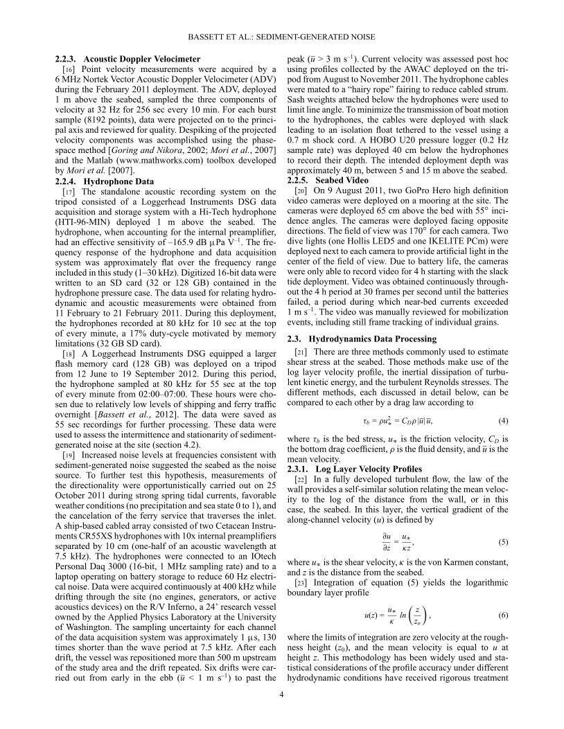
[10] The study site is located in Admiralty Inlet, PugetSound, Washington (USA). The majority of the tidalexchange between Puget Sound and the Strait of Juan deFuca occurs in Admiralty Inlet, resulting in currents inexcess of 3.0 m s–1 [Polagye and Thomson, 2013]. A mapof Admiralty Inlet, Puget Sound, and the bathymetry areincluded in Figure 1.

[11] Classification of the seabed at the site is difficultdue to the water depth (>50 m), lack of ambient light,and strong currents. Acoustic profiling undertaken in 2009[Snohomish PUD, 2012] indicated a hard substrate, butcould not provide a more accurate classification. Transectsby a remotely operated vehicle (ROV) [Greene, 2011, anappendix to Snohomish PUD [2012]], are the most compre-hensive data set currently available. Grain size distributionsin the ROV survey were determined using ranging lasersseparated by 10 cm on the ROV housing. Grain size classifi-cation was made based on a modified Wentworth scale whereD is the characteristic diameter of the grain [Wentworth,1922]. The reported bottom types included a combinationof small boulders (D = 25.6–40.0 cm), cobbles (D =6.4–25.6 cm), pebbles (D = 3.2–6.4 cm), gravel (D = 0.2–3.2 cm), and coarse sand (D = 0.05–0.2 cm). Greene [2011]reports two dominant substrate types within the immediatevicinity (O(100 m)) of the study site: a soft, unconsolidatedbimodal distribution of pebble and gravel likely to be mobi-lized during strong currents, and a mix of cobble (35–50%),pebbles (<35%), and small boulders. Small boulders and

2


Figure 1. (a) A map of the Salish Sea. The red box highlights northern Admiralty Inlet. (b) A map ofnorthern Admiralty Inlet, Puget Sound, and the deployment site. The deployments are represented by awhite square (the Feb 2011 and June–Sept 2012 locations are indistinguishable at this scale) and graylines (Oct 2011 drifts).

cobbles were typically well rounded and moderately toheavily encrusted with sponges, bryozoans, barnacles, tubeworms, and algae, suggesting these substrates to be sta-tionary [Greene, 2011]. Finer-grain constituents have beenlargely winnowed from the surface pavement. Where peb-bles, gravel, and coarse sand were reported, they wereunencrusted. Farther from the locations where instrumenta-tion packages were deployed, in areas with weaker currents,pebbles were encrusted. In general, the substrate was uncon-solidated and smaller constituents were easily moved bythe ROV.

2.2. Data Collection[12] Oceanographic and acoustics measurements were

obtained using a combination of autonomous instrumen-tation packages built around Sea Spider tripods (Ocean-science, Ltd.) and ship-based cabled instruments. Threeprimary deployments were used in data analysis and twoadditional deployments were used to obtain supplemen-tary information. All deployments were in northeasternAdmiralty Inlet, near Whidbey Island. A list of the deploy-ments, locations, and instruments used in the analysis areincluded in Table 1. The relationship between noise levelsand hydrodynamics are based on the February 2011 deploy-ment (tripod at depth of 55 m). October 2011 (shipboardcabled drifts) data were used to assess the directionalityand June–September 2012 data (tripod at depth of 54 m)were used to assess the intermittency and stationarity ofsediment-generated noise.2.2.1. Acoustic Wave and Current Profiler

[13] A 1 MHz Nortek Acoustic Wave and Current pro-filer (AWAC) was used to measure currents from 1.05 to26.05 m above the seabed. The AWAC profiled the water

column in 0.5 meter bins at a frequency of 1 Hz during theFebruary 2011 deployment. Mean current magnitude anddirection were calculated using 5 min ensembles. As shownin Thomson et al. [2012], this ensemble period filtersout the majority of turbulence. The standard error fora single ping measurement, also referred to as “Dopplernoise,” was �u = 0.224 m s–1. The uncertainty ineach velocity bin as a function of �u and the numberof raw pings, N, in the ensemble is u ˙ �up

N[Brumley

et al., 1991]. For 5 min ensembles, the resulting uncer-tainty was 0.013 m s–1, a value two orders of magni-tude smaller than observed maximum non-turbulent currents(i.e., mean currents).

[14] Current profiles obtained using the AWAC duringthe August–November 2011 deployment were used to deter-mine current velocities during shipboard drift surveys on25 October 2011. Each profile was based on 30 sec averagesobtained every 60 sec in 1 meter spatial bins. The resultinguncertainty in the currents was 0.045 m s–1.2.2.2. Acoustic Doppler Current Profiler

[15] A 470 kHz Nortek Continental Acoustic DopplerCurrent Profiler (ADCP) was used to measure currents from1.69 to 49.69 m above the seabed in 1 m bins during theJune–September 2012 deployment. Mean current magnitudeand direction were calculated using 1 min ensembles. Linearinterpolations of the February 2011 data were used to calcu-late a scalar factor to convert the velocity in the lowest bin ofthe June–September 2012 data (1.69 m) to the expected near-bed velocity at the same height as the February 2011 data(1.05 m). Current profiles were used only to approximatenear-bed currents for the purposes of studying the intermit-tency and stationarity of sediment-generated noise duringstrong currents.

Table 1. Deployments, Locations, and Instrument Packages Used in this Study

Deployments Location Instruments Purpose

11–21 Feb 2011 48 09.120ıN, 122 41.152ıW ADV, AWAC, Hydrophones (�2) Bed stress and ambient noise9 Aug 2011 48 09.124ıN, 122 41.195ıW GoPro Hero (�2), Dive lights (�4) Video of seabed10 Aug–14 Nov 2011 48 9.148ıN, 122 41.305ıW AWAC Current profiles during drift survey25 Oct 2011 Drifts Cabled hydrophones (�2) Ambient noise

Pressure logger Hydrophone depth12 June–19 Sept 2012 48 09.172ıN, 122 41.171ıW ADCP, Hydrophone Current profiles and ambient noise

3


2.2.3. Acoustic Doppler Velocimeter[16] Point velocity measurements were acquired by a

6 MHz Nortek Vector Acoustic Doppler Velocimeter (ADV)during the February 2011 deployment. The ADV, deployed1 m above the seabed, sampled the three components ofvelocity at 32 Hz for 256 sec every 10 min. For each burstsample (8192 points), data were projected on to the princi-pal axis and reviewed for quality. Despiking of the projectedvelocity components was accomplished using the phase-space method [Goring and Nikora, 2002; Mori et al., 2007]and the Matlab (www.mathworks.com) toolbox developedby Mori et al. [2007].2.2.4. Hydrophone Data

[17] The standalone acoustic recording system on thetripod consisted of a Loggerhead Instruments DSG dataacquisition and storage system with a Hi-Tech hydrophone(HTI-96-MIN) deployed 1 m above the seabed. Thehydrophone, when accounting for the internal preamplifier,had an effective sensitivity of –165.9 dB �Pa V–1. The fre-quency response of the hydrophone and data acquisitionsystem was approximately flat over the frequency rangeincluded in this study (1–30 kHz). Digitized 16-bit data werewritten to an SD card (32 or 128 GB) contained in thehydrophone pressure case. The data used for relating hydro-dynamic and acoustic measurements were obtained from11 February to 21 February 2011. During this deployment,the hydrophones recorded at 80 kHz for 10 sec at the topof every minute, a 17% duty-cycle motivated by memorylimitations (32 GB SD card).

[18] A Loggerhead Instruments DSG equipped a largerflash memory card (128 GB) was deployed on a tripodfrom 12 June to 19 September 2012. During this period,the hydrophone sampled at 80 kHz for 55 sec at the topof every minute from 02:00–07:00. These hours were cho-sen due to relatively low levels of shipping and ferry trafficovernight [Bassett et al., 2012]. The data were saved as55 sec recordings for further processing. These data wereused to assess the intermittence and stationarity of sediment-generated noise at the site (section 4.2).

[19] Increased noise levels at frequencies consistent withsediment-generated noise suggested the seabed as the noisesource. To further test this hypothesis, measurements ofthe directionality were opportunistically carried out on 25October 2011 during strong spring tidal currents, favorableweather conditions (no precipitation and sea state 0 to 1), andthe cancelation of the ferry service that traverses the inlet.A ship-based cabled array consisted of two Cetacean Instru-ments CR55XS hydrophones with 10x internal preamplifiersseparated by 10 cm (one-half of an acoustic wavelength at7.5 kHz). The hydrophones were connected to an IOtechPersonal Daq 3000 (16-bit, 1 MHz sampling rate) and to alaptop operating on battery storage to reduce 60 Hz electri-cal noise. Data were acquired continuously at 400 kHz whiledrifting through the site (no engines, generators, or activeacoustics devices) on the R/V Inferno, a 24’ research vesselowned by the Applied Physics Laboratory at the Universityof Washington. The sampling uncertainty for each channelof the data acquisition system was approximately 1 �s, 130times shorter than the wave period at 7.5 kHz. After eachdrift, the vessel was repositioned more than 500 m upstreamof the study area and the drift repeated. Six drifts were car-ried out from early in the ebb (u < 1 m s–1) to past the

peak (u > 3 m s–1). Current velocity was assessed post hocusing profiles collected by the AWAC deployed on the tri-pod from August to November 2011. The hydrophone cableswere mated to a “hairy rope” fairing to reduce cabled strum.Sash weights attached below the hydrophones were used tolimit line angle. To minimize the transmission of boat motionto the hydrophones, the cables were deployed with slackleading to an isolation float tethered to the vessel using a0.7 m shock cord. A HOBO U20 pressure logger (0.2 Hzsample rate) was deployed 40 cm below the hydrophonesto record their depth. The intended deployment depth wasapproximately 40 m, between 5 and 15 m above the seabed.2.2.5. Seabed Video

[20] On 9 August 2011, two GoPro Hero high definitionvideo cameras were deployed on a mooring at the site. Thecameras were deployed 65 cm above the bed with 55ı inci-dence angles. The cameras were deployed facing oppositedirections. The field of view was 170ı for each camera. Twodive lights (one Hollis LED5 and one IKELITE PCm) weredeployed next to each camera to provide artificial light in thecenter of the field of view. Due to battery life, the cameraswere only able to record video for 4 h starting with the slacktide deployment. Video was obtained continuously through-out the 4 h period at 30 frames per second until the batteriesfailed, a period during which near-bed currents exceeded1 m s–1. The video was manually reviewed for mobilizationevents, including still frame tracking of individual grains.

2.3. Hydrodynamics Data Processing[21] There are three methods commonly used to estimate

shear stress at the seabed. Those methods make use of thelog layer velocity profile, the inertial dissipation of turbu-lent kinetic energy, and the turbulent Reynolds stresses. Thedifferent methods, each discussed in detail below, can becompared to each other by a drag law according to

�b = �u2� = CD� |u| u, (4)

where �b is the bed stress, u� is the friction velocity, CD isthe bottom drag coefficient, � is the fluid density, and u is themean velocity.2.3.1. Log Layer Velocity Profiles

[22] In a fully developed turbulent flow, the law of thewall provides a self-similar solution relating the mean veloc-ity to the log of the distance from the wall, or in thiscase, the seabed. In this layer, the vertical gradient of thealong-channel velocity (u) is defined by

@u@z

=u��z

, (5)

where u� is the shear velocity, � is the von Karmen constant,and z is the distance from the seabed.

[23] Integration of equation (5) yields the logarithmicboundary layer profile

u(z) =u��

ln�

zzo

�, (6)

where the limits of integration are zero velocity at the rough-ness height (z0), and the mean velocity is equal to u atheight z. This methodology has been widely used and sta-tistical considerations of the profile accuracy under differenthydrodynamic conditions have received rigorous treatment

4

www.mathworks.com


[Heathershaw, 1979; Gross and Nowell, 1983; Grant et al.,1984; Green, 1992; Lueck and Lu, 1997].

[24] The uncertainty of the shear velocity is related to thelog layer fit by

�u� = t˛/2,n–2

�1

n – 2

�1 – R2

R2

��1/2

, (7)

where t˛/2,n–2 is the Student’s t-statistic for a confidence level˛ with n degrees of freedom and R2 is the coefficient ofdetermination [Gross and Nowell, 1983]. Since the uncer-tainty in density is negligible (CTD measurements using aSeabird 16plus recorded density variations of less than 2 kgm–3, relative to a nominal value of 1024 kg m–3 during theFebruary deployment), the uncertainty in bed stress fromequation (4) is only dependent on the uncertainty in fric-tion velocity. The propagation of uncertainty from frictionvelocity to the bed stress is calculated according to

��b = 2�b�u�u�

, (8)

where �u� is the error calculated using equation (7). Rea-sonable confidence intervals for shear velocity and bedstress calculations are contingent upon high coefficients ofdetermination for the log layer fits.

[25] In this study, log layer fitting followed the meth-ods discussed in Lueck and Lu [1997] and was applied toAWAC data collected during February 2011. For each pro-file, a least squares fit to the bottom bins of the profile (1.05to 4.05 m) was first calculated. From the bottom bins, newfits were calculated adding one velocity bin each iterationuntil the profile extended to 25 m from the seabed. The loglayer depth (z) was defined as the depth at which the high-est R2 value was identified. Only those fits with maximumR2 exceeding 0.95 were retained. This most often was absentduring transitions between flood and ebb tides, so data withnear-bed currents below 0.5 m s–1 were not analyzed.2.3.2. Reynolds Stress

[26] In a turbulent flow, the velocity is described by(ui + u0i), where ui is the mean velocity, u0i is the velocityfluctuation, and the index (i) denotes the velocity compo-nent. The instantaneous kinematic stress, based on velocityfluctuations in the vertical and along channel flow, is writtenas u0w0, and is calculated as the covariance of the compo-nents. By assuming a constant stress layer, the bed stress isobtained from the Reynolds stress by

�b = –�u0w0, (9)

where � is the fluid density. In general, Reynolds stress cal-culations are noisy because the variance of each flow compo-nent is large relative to the mean [Gross and Nowell, 1983].Rigorous treatment of the Reynolds stress calculations andshear stress estimates is presented in both oceanographic andatmospheric literature [Tennekes, 1973; Heathershaw, 1979;Gross and Nowell, 1983; Heathershaw and Thorne, 1985;Trowbridge et al., 1999; Lu et al., 2000].

[27] Turbulent Reynolds stresses were calculated fromADV data for each 5 min interval directly from the covari-ance of along-channel and vertical velocity componentsaccording to equation (9). The correlation coefficient andcoefficient of determination for each Reynolds stress calcu-lation were calculated. An autocorrelation of the Reynolds

stress was used to identify the decorrelation time scales,which were generally on the order of 1 sec. The number ofdegrees of freedom was calculated as the full sample length(256 sec) divided by the event duration (twice the decor-relation time) [Gross and Nowell, 1983]. The degrees offreedom, t-statistic, and R2 value were used in equation (7) tocalculate the uncertainty in the shear velocity which is prop-agated to the bed stress. To remove spurious data, when therelative Reynolds stress uncertainties exceeded 100% (datawith low velocities when the variance of the velocities fluc-tuations was large relative to the mean velocity), the datawere excluded from analysis. As for the log layer method,the excluded data were associated with the transition flows.2.3.3. Inertial Dissipation

[28] Kolmogorov hypothesized large, turbulent eddiestransfer energy to increasingly smaller eddies until vis-cous dissipation takes place at scales on the order of theKolmogorov length. Although the largest scales of turbu-lence may not be isotropic, Kolmogorov noted that theenergy cascade through the inertial subrange from the large,energy containing eddies to dissipation scales consists ofisotropic turbulent eddies. For an isotropic turbulent energycascade, the frequency spectrum of turbulent kinetic energyis described by

S( f ) = ˛�2/3f –5/3�

u2

�2/3

, (10)

where ˛ is a constant taken to be 0.69 when using the verticalvelocity spectrum, � is the dissipation rate, f is the frequency,and u is the mean along-channel velocity at a given depth.Dissipation can be calculated by fitting a line to the portionof the turbulence spectrum with the f –5/3 slope.

[29] For a fully developed, unstratified flow with negligi-ble advection, the turbulent kinetic energy budget reducesto a balance between the production and dissipation ofturbulence. This balance is described by

� = –u0w0@u@z

, (11)

where � is the dissipation rate and u0w0 is the kinematicstress. By assuming a constant stress layer and substitutingthe friction velocity for the kinematic stress (u2

� = –u0w0),the bed stress can be found by

�b = �(��z)2/3, (12)

where � is the von Karmen constant.[30] The dissipation of turbulent kinetic energy was cal-

culated using the turbulent velocity spectrum for each ADVburst. Each 256 sec record was broken up into individualwindows with 1024 data points and an overlap of 50%.After removing the mean, windows were multiplied by aHann function and rescaled to preserve variance. An ensem-ble average of all windows in each burst produced the finalspectrum. The first window was removed because the over-lapping process resulted in zero padding of the first window.The resulting spectra have 40 degrees of freedom [Priestley,1981]. The 95% confidence interval, obtained from a chi-squared distribution, is 0.61 S( f ) < S( f ) < 1.48 S( f ) whereS( f ) is the turbulence spectrum.

[31] The vertical velocity spectrum was used to estimatethe dissipation rate of turbulent kinetic energy because the

5


ADV beam geometry resulted in less noise in the verti-cal direction. The vertical velocity spectrum was multipliedby f 5/3 to obtain a flat spectrum in the inertial subrange.The slope of the spectrum was calculated over a seriesof frequency ranges: 0.25–1, 0.5–2, 1–6, 4–8, 8–12, and12–16 Hz. The fits for the frequency ranges contained either25, 65, or 81 points. The frequency range with the minimumslope was defined as the inertial subrange. The dissipationwas calculated by setting the mean value over this rangeequal to ˛�2/3

� u2�

�2/3 and solving for �. Uncertainties werecalculated by finding the standard deviation and 95% con-fidence intervals for the spectrum values in the frequencyrange of the fit. The relative uncertainty bounds for thebed stress, obtained by propagating the uncertainty in thedissipation rate through equations (10) and (12), are

��b =

s4�2�2z2

9 (��z)2/3 (��)2, (13)

where the uncertainties of all of the variables, with theexception of the dissipation rate, are negligible.

[32] On the tripod, the ADV was deployed immedi-ately adjacent to a second hydrophone shrouded in ashield intended to reduce measurements of flow-noise(10 cm diameter, 43.2 cm height). The sampling volume wasapproximately 15 cm from the flow shield. A projection ofthe wake in the direction of the flow revealed that when ebbvelocities exceeded 0.5 m s–1, the ADV sampling volumewas immediately downstream of the flow shield. As a result,the measurements from the ADV during ebb tides may havebeen compromised by the wake and are not presented.2.3.4. Drag Coefficients

[33] The drag coefficients for flood and ebb tides and theirrespective uncertainties were calculated by regressing theshear velocity versus the mean current squared. The regres-sions were performed in both log space and linear space.In linear scale calculations large shear velocities are empha-sized whereas log scale calculations emphasize small shearvelocities [Lueck and Lu, 1997]. For comparison, the dragcoefficients were calculated for Reynolds stress and iner-tial dissipation techniques. For both techniques, equation (4)governs the relationship between the calculated bed stresses,shear velocities, and drag coefficients.

2.4. Acoustic Data Processing[34] Acoustics data were processed using standard signal

processing techniques. For the primary data set of Febru-ary 2011, the digitized signals were converted to voltage andsplit into windows containing 216 data points with a 50%overlap. For each window, the mean voltage was removed,a Hann function applied, and the signal scaled to preservevariance before applying a Fast Fourier Transform (FFT).Calibration curves were applied to convert voltage spectrato pressure spectra. Ensemble averages of the windowedpressure spectra were calculated to improve the underly-ing statistics in each 10 sec recording (ensemble size of23, bandwidth of 1.2 Hz). The one-third octave band soundpressure levels (TOLs) [1–25 kHz center frequencies] werecalculated by integrating under the spectra.

[35] The June–September 2012 data were processed intwo ways to support the analysis of stationarity and inter-mittency. First, to produce spectrograms with high temporal

resolution (�t � 0.025 seconds), data were processed using212 data points (bandwidth of 19.5 Hz). Spectra and broad-band sound pressure levels (2–20 kHz) were also calculatedin 1 sec windows (ensemble size of 38). These data wereused to highlight mobilization events in the direct vicinityof the hydrophones. Stationarity was investigated by sub-sampling each 55 sec recording to obtain five total signals(4 subsamples and the original). The subsampled signalswere the first 1, 5, 10, and 30 sec of each recording. Thesefour signals and the entire 55 sec recording were used tocalculate the TOLs (ensemble sizes: 40, 196, 391, 1172,2344). The resulting TOLs were used to compare the resultsof different duty cycles by subtracting the TOLs of the 55sec recordings from those calculated using the 1, 5, 10, and30 sec subsamples. A distribution of the results, using 0.5decibel bins, was calculated for three different frequencies(4, 8, and 16 kHz) during all periods when sediment-generated noise occurs and in one velocity bin (ebb currentsbetween 1.15–1.35 m s–1).2.4.1. Frequency Dependence ofSediment-Generated Noise

[36] The equivalent grain diameter for the particles in thisstudy were calculated using the theoretical expression in theform of equation (3), based on a fit to equation (2), for sitespecific material properties. Available information about thecomposition of the seabed note a mix of plutonic and meta-morphic rocks [Greene, 2011]. Using the material propertiesof basalt (� = 2500 kg m–3, E = 60 GPa, and � = 0.15)the theoretical centroid frequencies for equivalent grain sizeswere related by

fc =206D0.9 . (14)

[37] The resonant frequencies for equivalent grain sizespresent at the site did not vary significantly from the resultsobtained for basalt if other possible material types wereassumed. Specifically, the material properties of granite,rhyolite, quartize, gneiss, and slate all resulted in equiva-lent grain diameters within 15% of those obtained under anassumption of basalt for a given frequency. This differencewas relatively small when compared to the distributions ofgrain sizes which spans nearly two orders of magnitude fromcoarse sand to cobbles.2.4.2. Directionality

[38] The directionality of sound can be determined usingcross-spectral methods. In an array, the phase (12) rela-tionship between two independent signals can be calculatedwhen coherence (�12) values are statistically significant. Thesquared coherence is calculated by

�212 =

|S12( f )|2

S11( f )S22( f ), (15)

where S12 is the cross-spectrum, S11 is the autospectrum ofthe first signal, and S22 is the autospectrum of the secondsignal [Priestley, 1981]. Each component of equation (15),as well as the coincident and quadrature spectra, is cal-culated from the October 2011 drift study according tothe previously identified signal processing techniques (i.e.,windowing and averaging) prior to the calculation of thecoherence. Data windows contained 215 points with a 50%overlap, resulting in spectra with a bandwidth of 39.1 Hz.Processed data were used to calculate the phase lags between

6


the two hydrophones at frequencies of interest during strongcurrents to indicate whether the noise was generated aboveor below the hydrophones (section 2.4.2). Mean squaredcoherence was calculated for 10 sec sequences (ensemblesize 180). Phase lags were calculated with respect to thedeeper hydrophone such that a negative phase lag indicatesnoise generated below the array. The maximum uncertaintyof the phase attributable to the DAQ, based on the samplinguncertainty, was less than 3ı at the frequencies of interest.

[39] Confidence levels for coherence represent the lowestmean-squared coherence that is expected to occur randomly.Thompson [1979] calculated the significance of squared-coherence values and compared the results to Monte Carlosimulations. The work demonstrated that the confidenceinterval is related to the number of degrees of freedom in thecalculations for the mean-squared coherence by

�21–˛ = 1 – ˛[ 2

�–2 ], (16)

where 1 – ˛ is the confidence level and � is the equiva-lent number of degrees of freedom for the cross-spectrum[Priestley, 1981, Table 6.2].

[40] The phase relationships between signals are calcu-lated using coincident and quadrature spectra. The phase lag,as a function of frequency, between signal one and signaltwo is calculated by

12( f ) = tan–1�

–Q12( f )C12( f )

�, (17)

where 12 is the phase lag, Q12 is the quadspectrum, and C12is the cospectrum [Priestley, 1981]. Phase lag estimates aresuspect, although not necessarily incorrect, when squared-coherence does not exceed the desired confidence level.

[41] For sediment-generated noise and a vertical linearray of two hydrophones measuring collisions directlyin-line with the array (i.e., collisions directly below thehydrophones for a vertical array), the estimated phase lagbetween two measurements is related to the acoustic fre-quency (f), speed of sound (c), and the separation distancebetween the hydrophones (L). As frequency increases, thephase lag of the signal is expected to increase linearly for alocalized source directly below the array. Under ideal condi-tions, the phase lag relationship, in degrees, for the verticalline array is described by

Q12( f ) = 360�

f Lc

�, (18)

where Q denotes the idealized phase lag for a source directlybelow a vertical array. In practice, the incidence angle (thelocation of the source relative to the line array) and theorientation angle for a line array (i.e., angle from ver-tical) are important. In both cases, deviations from theideal case reduce the measured phase lag relative to theidealized value.2.4.3. Noise Level Regressions

[42] To assess the relationship between near-bed currentvelocities and sediment-generated noise, regressions wereperformed using terms developed from the one-third octaveband sound pressure levels and the near-bed velocity cubed.The velocity-cubed metric was used because it provides alogical balance between the units of sound and velocity.

Using the plane wave assumption, the TOLs can be eas-ily converted to an acoustic intensity (i.e., power per unitarea). Likewise, the velocity-cubed metric, normalized by anarea of 1 m2, can be readily interpreted as a rate of energyinput (i.e., power) per unit area. Thus, the regression coef-ficients may be thought of as representing of the efficiencywith which hydrodynamic power is converted to acous-tic power through the mobilization of sediment. The finalequations and units for the terms used in the regression aredescribed by

Pa,m = 10 log�

10TOLm

10p2o�c

�[dB re 1 W m–2], (19)

Ph =12�U3

A[W m–2], (20)

where Pa,m is the acoustic power in the mth TOL, Ph is thenear-bed hydrodynamic power, po is the underwater refer-ence pressure (1�Pa), � is the density (1024 kg m–3), c isthe sound speed (1490 m s–1), U is the along-channel, near-bed, mean velocity, and A is the area (1 m2). The regression,described by

Pa,m = am + bmPh, (21)

provides the coefficients am and bm, which may be con-ceptually thought of as the background noise intensity(y-intercept, dB re 1W m–2) and the efficiency with whichthe power input to the seabed by currents is converted tosound (slope, dB re 1W m–2 per unit increase in near-bed hydrodynamic power). We note that this should beconsidered only a conceptual framework to give physicalcontext to the regression coefficients since, for example,the power input to the seabed is likely related to U3. Onecould construct a similar conceptual framework around a U2

dependence on the basis of drag forces acting on the seabed.In practice, we found that the use of a U3 versus U2 has lit-tle effect on the statistical power of the derived regressioncoefficients.

[43] Prior to estimating the regression coefficients, Auto-matic Identification System data (section 2.5.1) were used toremove measurements with co-temporal vessel traffic within10 km of the site. For the remaining data, mean measuredTOLs were calculated in 0.1 m s–1 velocity bins. Only peri-ods when TOLs exceed the quiescent mean (TOL for |U| <0.3 m s–1) by 3 dB or more were used in the regression. Aseparate regression was performed for each one-third octaveband. The lowest velocity bin in which the 3 dB increasewas noted for each TOL was considered the critical veloc-ity. This critical velocity was used to estimate the criticalshear stress for mobilization of the equivalent grain sizesaccording to the inversion of the spectrum. It should be notedthat defining the critical shear stress as the point at whichTOLs have increased by 3 dB is inherently conservative.Miller et al. [1977] notes that the threshold should be definedas the conditions (bed stress) just lower than that whichresults in incipient motion. By relying on increases in soundintensity above ambient noise levels (which are attributed toother sources) to identify critical bed stresses, the thresholdsreported here differ from established definitions. However,no other method to identify incipient motion is suitable forthese indirect observations.

7


[44] To access the regression quality, the R2 values arecalculated fits to velocity bin-averaged TOLs according toequations (19)–(21). Similarly, near-bed currents were usedto create a reconstruction predicted TOLs using the regres-sion results according to equation (22). The R2 values werethen calculated using observed TOLs and the TOLs pre-dicted from the regression coefficients. These R2 valuesrepresent the degree to which mean noise levels in a one-third octave band were dependent on the near-bed currents.To qualitatively demonstrate this dependence, the regressioncoefficients were used to construct a 24-hour spectrogram ofnoise levels from 1-25 kHz. Using the regression, the outputwas converted to TOLs according to

TOLm(t) = 10log10

��cp2

o10

am10

�+

12

bm�U3 [dB re 1�Pa], (22)

with terms as defined in equations (19)–(21). The regressioncoefficients were only applied to conditions when mean cur-rents exceeded the critical values. When near-bed velocitieswere below the critical value, the TOL values were taken tobe only the first term of equation (22) (i.e., mean ambientnoise during weak currents).

2.5. Exclusion of Other Noise Sources2.5.1. Vessel Noise

[45] While noise from vessel traffic is often considered atfrequencies lower than those of interest for this study (i.e., <1 kHz), Bassett et al. [2012] identifies vessel traffic noise asan important contributor to ambient noise at the frequenciesconsidered in this study. Consequently, a field assessmentof sediment-generated noise from a location with high ves-sel traffic density needs to exclude periods when vesseltraffic might substantially contribute to ambient noise. AnAutomatic Identification System (AIS) was deployed at theAdmiralty Head Lighthouse in Fort Casey State Park, lessthan 1 km from the site, to log real-time vessel traffic data.An AIS receiver (Comar AIS-2-USB) and data acquisitioncomputer recorded incoming AIS strings and appended themwith a timestamp using a Python script written to recordand archive the data. Data were post-processed using aPython package (NOAA data version 0.43) [Schwehr, 2010].This process converted raw AIS transmissions into ASCIIformat text.

[46] Vessel coordinates and speed over ground wereextracted from each AIS string. The coordinates were usedto calculate the radial distance from the vessel to thehydrophone. To prevent vessel noise from biasing analysisof sediment-generated noise, all recordings of ambient noisewith an AIS transmitting vessel in transit (vessel speed >0.05 m s–1) within 10 km of the site were excluded. In addi-tion, acoustic data were reviewed manually and recordingswith signals consistent with vessel traffic were also removed.This can occur when vessels that do not consistently trans-mit AIS information, such as military vessels, transit the site.Due to low signal-to-noise ratios relative to flow-inducedpseudosound, such events were difficult to identify duringperiods of strong currents and were not removed from thedata set [Bassett, 2010]. As demonstrated in section 3.2, thisshould not have an impact on the results because peak lev-els from vessel noise are exceeded by sediment-generatednoise at the frequencies under consideration duringstrong currents.

2.5.2. Pseudosound[47] Hydrodynamic flow-noise, or pseudosound, is a

result of turbulent pressure fluctuations measured byhydrophones. This non-propagating noise is a low-frequencyphenomenon and should not be included in a discussionof ambient noise. Studies have reported flow-noise fromoceanic turbulence at frequencies as high as 110 Hz [Gobatand Grosenbaugh, 1997]. In a series of papers on hydro-dynamic flow-noise and wind screen noise, Strasberg notedthat the frequency of noise generated by turbulent pres-sure fluctuations is related to the wavelengths of the spatialvelocity fluctuations and the mean velocity [Strasberg, 1979,1984, 1988]. The upper frequency limit for flow-noise isdescribed by f = |u| –1

o , where u is the mean current and ois the Kolmorgorov microscale, the smallest scale that canoccur before viscosity damps out the turbulent fluctuations.The microscales are related to the dissipation rate by o =(�3/�)0.25 where � is the kinematic viscosity and � is the dis-sipation rate. For an extreme example, a peak dissipation rateof 0.002 m2 s–3, consistent with previous findings at the sitein this study [Thomson et al., 2012] is used. This dissipationrate implies bed stresses on the order of 10 Pa and suggestsa microscale of 0.2 mm. With near-bed currents on the orderof 2 m s–1, the peak at the site, the maximum theoreticalfrequency at which flow-noise is expected is approximately10 kHz. However, when the size of the hydrophone ele-ment is larger than the turbulent microscales, as is the casein this extreme example where the hydrophone diameter(0.019 m) is nearly two orders of magnitude larger than theKomolgorov microscale, the signal of pseudosound at thesefrequencies will be attenuated. This attenuation is a resultof phase changes across the hydrophone that cause the pres-sure differences to partially cancel [Strasberg, 1979, 1984],such that the measurable limit of flow-noise is lower than thetheoretical maximum. For peak conditions, the scales of tur-bulence of the same size as the hydrophone would result innoise up to 100 Hz.

[48] The basic characteristics of the acoustic spectraduring periods with strong currents suggest that flow-noise is not the source of the increases above 1 kHz.Figure2 includes an example spectrum from a period with anear-bed velocity of 1.6 m s–1. Between 1–2 kHz noise lev-els in this example, and in general for periods with strongcurrents, are within the range of observed noise levels dur-ing slack tide conditions (section 3.2). Furthermore, above1 kHz, the observed spectra diverge from the observed andexpected “red” spectrum associated flow-noise. Given thatthe analysis in this study focuses on frequencies greater than1 kHz, we conclude that pseudosound is not of primaryimportance in this study and is “masked” by propagatingambient noise in the frequency range of interest.

3. Results[49] There is a strong dependence of observed noise lev-

els on near-bed currents (Figure 3). The combination ofacoustic and hydrodynamic measurements are used furtherto analyze the relationships between sediment-generatednoise levels and the near-bed currents. As for the methods,hydrodynamic results precede acoustic results. Followingthe hydrodynamic results, sections discussing the direc-tionality, intermittency, and stationarity of observed noise

8


101 102 103 10495

100

105

110

115

120

125

130

Frequency (Hz)

TO

L (

dB

re

1μP

a)

PseudosoundSediment−generatednoise

Figure 2. An example spectrum typical of acoustic mea-surements during strong currents. In this example withcurrents of 1.6 m s–1, at frequencies below 1 kHz, the spec-trum is “red” as expected for measurements of flow-noise.Above 1 kHz, the patterns are not consistent with flow-noisemeasurements, but rather with sediment-generated noise.

are presented along with a comparison of the observednoise measurements during comparable conditions duringthe three deployments. These relationships are summarizedusing a frequency dependent regression.

3.1. Hydrodynamics[50] Bed stresses obtained via the log layer, Reynolds

stress, and inertial dissipation techniques are plotted againstthe mean current for the bottom velocity bin (1.05 m) inFigure 4. Each measurement has unique error bars obtainedaccording to the methodology discussed in section 2.3. Forclarity, a single relative uncertainty representative of eachmethod is included.

[51] A total of 75% of log layer fits meet the R2 >0.95 criterion. Periods when R2 values are lower than 0.95are typically associated with slack currents. When currentsexceed 1 m s–1, 99% of log layer fits have an R2 valueexceeding 0.95. No fits with R2 values greater than 0.95 havefewer than 10 degrees of freedom (i.e., the log layer height isalways at least 10 bins high). The propagation of the uncer-tainty to the shear stress calculation results in a maximumuncertainty of ˙36%, although for currents greater than1 m s–1, the maximum uncertainty in shear stress is typicallyless than ˙10%.

[52] Representative uncertainties for the Reynolds stressmethod are evaluated using the cumulative probability den-sity of uncertainties (not shown). Fifty percent of uncertain-ties for this method are ˙15% or less. A more conservativerepresentative uncertainty for bed stresses of ˙35%, the95% value from the distribution, is chosen. For the iner-tial dissipation method, the representative uncertainty ischosen as the 95% value from a cumulative probability den-sity function of relative uncertainties of the bed stress. Therepresentative uncertainty is ˙27%.

[53] Mean bed stresses, roughness length calculated bythe log layer fits, and drag coefficients obtained usingthe Reynolds stress and inertial dissipation techniques areincluded for 0.25 m s–1 velocity bins in Table 2. Themethods show good agreement and are in closest agreementwhen currents exceed 1 m s–1. As discussed in section 3.2,

these are the same periods in which significant increases ofambient noise are observed. Figure 4 also includes plots ofthe bed stresses estimated by the Reynolds stress methodversus the inertial dissipation and log layer methods. Duringflood tides there is good agreement between the results for allthree methods. During ebb tides the log layer and Reynoldsstress methods agree well. As mentioned in section 2.3, thedissipation rate of turbulent kinetic energy during ebb cur-rents are not included in Table 2 and Figure 4, because themeasurements may have been compromised by the wakeof another instrument. Bed stresses calculated by all meth-ods are found to exceed 1 Pa at the site for currents greaterthan 0.5 m s–1. Above 1 m s–1 mean bed stresses areapproximately 5 Pa, and peak bed stresses exceed 20 Pa.

[54] The drag coefficient is calculated on both linear andlog scales for comparison. Drag coefficients calculated usingReynolds stresses for the log and linear fits are indistinguish-able with values of 0.0039 and 0.0045 for ebb and floodtides. The drag coefficients calculated using the Reynoldsstress and inertial dissipation techniques during flood tidesare comparable to values obtained at other sites with coarse-grained beds [Williams et al., 1989; Thorne et al., 1989;Lueck and Lu, 1997]. Based on the good agreement betweenthe flood tide drag coefficients and measured data, the dragcoefficient (CD = 0.0044, linear scale) is applied later tocalculate critical shear stresses.3.2. Acoustics3.2.1. Frequency Dependence ofSediment-Generated Noise

[55] When noise levels are considered across all stages ofthe tide, there are significant increases in noise levels relativeto near-quiescent conditions above 1 kHz that are correlatedwith strong currents, as shown in Figure 5 for mean noisespectra in one-third octave bands in 0.2 m s–1 near-bed veloc-ity bins. Previous analysis of data from the same site providecontext for the increases in ambient noise attributed to themobilization of the bed. Bassett et al. [2012] presents ambi-ent noise levels, primarily associated with vessel traffic, for

−2 −1 0 1 20

5

10

15

20

25

TO

L −

TO

Lm

ean

,sla

ck (

dB

re

1μP

a)

Velocity (m s−1)

Fre

qu

ency

(kH

z)

1.00

1.25

1.60

2.00

2.50

3.15

4.00

5.00

6.30

8.00

10.00

10.25

16.00

20.00

25.00

Figure 3. TOLs with the mean quiescent noise levels (|U| <0.3 m s–1) subtracted versus near-bed current from 1 to25 kHz.

9


Drag Coefficient Dissipation

Reynolds Stress Log Layer

−2 −1 0 1 2

10−1

100

101

102

10−1 100 101 102 10−1 100 101 102

10−1

100

101

102

10−1

100

101

102

a)

u (m s−1)

τ b (

Pa)

τ b (

Pa)

τ b (

Pa)

Dissipation vs. Reynolds stress Log Layer vs. Reynolds stress

b) Ebb c) Flood

τb (Pa)τb (Pa)

Figure 4. (a) Measured bed stresses versus mean velocity using inertial dissipation, Reynolds stress,log layer fits, and a drag coefficient (calculated from Reynolds stress estimate). Error bars highlight therepresentative 95% uncertainty values for each method. The drag coefficients and their uncertainties arecalculated using a linear fit to Reynolds stress data (0.0039 for ebb tides and 0.0044 for flood tides,Table 2). (b) A comparison of bed stresses calculated by two methods for ebb tides. (c) A comparison ofbed stresses calculated by three methods for flood tides.

Table 2. Mean Bed Stresses in 0.25 m s–1 Velocity Bins for Reynolds Stress, Inertial Dissipation, and Log Layer Fit Techniques,Roughness Length Calculated by Log Layer Fits, and Drag Coefficients

�b (Pa) Velocity Bin (m s–1) 0–0.25 0.25–0.5 0.5–0.75 0.75–1.0 1.0–1.25 1.25–1.5 1.5–1.75 >1.75

Flood Reynolds Stress 0.2 0.8 2.0 3.6 6.4 8.6 14.3 15.7Inertial Dissipation 0.1 0.5 1.8 3.2 6.4 10.8 14.3 13.5

Log Layer - - 3.2 4.7 7.2 10.6 14.1 15.8Ebb Reynolds Stress 0.2 0.7 1.7 3.2 5.8 8.1 16.7 27.1

Inertial Dissipation - - - - - - - -Log Layer - - 3.2 5.0 8.7 12.4 17.3 19.8

z0 (m) Velocity Bin (m s–1) 0–0.25 0.25–0.5 0.5–0.75 0.75–1.0 1.0–1.25 1.25–1.5 1.5–1.75 >1.75

Flood Log Layer - - 0.018 0.008 0.007 0.007 0.005 0.005Ebb Log Layer - - 0.025 0.015 0.012 0.011 0.012 0.008

Linear Log

CD Ebb Flood Ebb Flood

Reynolds 0.0039˙ 0.0011 0.0044˙ 0.0002 0.0039˙ 0.0010 0.0045˙ 0.0001StressInertial - 0.0033˙ 0.0001 - 0.0042˙ 0.0001Dissipation

10


0 − 0.4 m s−1 0.85 − 1.05 m s−1 1.05 − 1.25 m s−1

1.25 − 1.45 m s−1 1.45 − 1.65 m s−1 > 1.65 m s−1

17.3 8.0 3.7 1.7 0.8 0.4

D (cm)

1 1080

90

100

110

120Ebb

TO

L (

dB

re

1μP

a)

Frequency (kHz)

17.3 8.0 3.7 1.7 0.8 0.4

1 1080

90

100

110

120

Frequency (kHz)

D (cm)

Flood

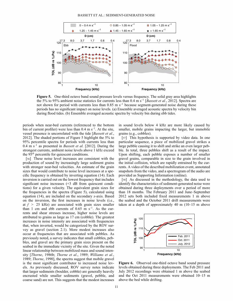
Figure 5. One-third octave band sound pressure levels versus frequency. The solid gray area highlightsthe 5% to 95% ambient noise statistics for currents less than 0.4 m s–1 [Bassett et al., 2012]. Spectra arenot shown for period with currents less than 0.85 m s–1 because segment-generated noise during theseperiods has no significant impact on noise levels. (a) Ensemble averaged acoustic spectra by velocity binduring flood tides. (b) Ensemble averaged acoustic spectra by velocity bin during ebb tides.

periods when near-bed currents (referenced to the bottombin of current profiler) were less than 0.4 m s–1. At the site,vessel presence is uncorrelated with the tide [Bassett et al.,2012]. The shaded portions of Figure 5 highlight the 5% to95% percentile spectra for periods with currents less than0.4 m s–1 as presented in Bassett et al. [2012]. During thestrongest currents, ambient noise levels above 1 kHz exceedthe 95th percentile for quiescent conditions.

[56] These noise level increases are consistent with theproduction of sound by increasingly large sediment grainswith stronger near-bed velocities. An estimate of the grainsizes that would contribute to noise level increases at a spe-cific frequency is obtained by inverting equation (14). Eachinversion is carried out on the lowest frequency that includessignificant noise increases (+3 dB from quiescent condi-tions) for a given velocity. The equivalent grain sizes forthe frequencies in the spectra (Figure 5), calculated usingequation (14), are included on the secondary x-axis. Basedon the inversion, the first increases in noise levels (i.e.,at f > 25 kHz) are associated with grain sizes smallerthan 1 cm and ebb currents of 0.65 m s–1. As the cur-rents and shear stresses increase, higher noise levels areattributed to grains as large as 17 cm (cobble). The greatestincreases in noise intensity are associated with frequenciesthat, when inverted, would be categorized by the ROV sur-vey as gravel (section 2.1). More modest increases alsooccur at frequencies that are associated with pebbles. Aspreviously noted, a survey indicates that small cobbles, peb-bles, and gravel are the primary grain sizes present on theseabed in the immediate vicinity of the site. Given the notedlinear relationship between mobilized mass and sound inten-sity [Thorne, 1986b; Thorne et al., 1989; Williams et al.,1989; Thorne, 1990], the spectra suggest that mobile gravelis the most significant contributor to increased noise lev-els. As previously discussed, ROV survey notes indicatethat larger sediments (boulder, cobble) are generally heavilyencrusted while smaller sediments (gravel, pebble, andcoarse sand) are not. This suggests that the modest increases

in sound levels below 4 kHz are more likely caused bysmaller, mobile grains impacting the larger, but immobilegrains (e.g., cobbles).

[57] This hypothesis is supported by video data. In oneparticular sequence, a piece of mobilized gravel strikes alarge pebble causing it to shift and strike an even larger peb-ble. In total, three pebbles shift as a result of the impact.Upon shifting, each pebble exposes a number of smallergravel grains, comparable in size to the grain involved inthe initial collision, which are rapidly entrained by the cur-rents. A video of the described mobilization event, annotatedsnapshots from the video, and a spectrogram of the audio areprovided as Supporting Information (online).

[58] As discussed in the methodology, the data used toidentify the characteristics of sediment-generated noise wereobtained during three deployments over a period of morethan 18 months. The February 2011 and June–September2012 sets both included fixed measurements 1 m abovethe seabed and the October 2011 drift measurements weretaken at a depth of approximately 40 m (10–15 m above

1 1090

100

110

120

TO

L (

dB

re

1μP

a)

Frequency (kHz)

Feb. 2011Oct. 2011July. 2012

Figure 6. Observed one-third octave band sound pressurelevels obtained during three deployments. The Feb 2011 andJuly 2012 recordings were obtained 1 m above the seabedand the Oct 2011 measurements were obtained 10–15 mabove the bed while drifting.

11


0 2 4 6 8 100

0.2

0.4

0.6

0.8

1

γ2

a)

99%

0 2 4 6 8 10−180

−90

0

90

180

φ 12 (d

eg)

Frequency (kHz)

b)Surface Noise

Seabed Noise

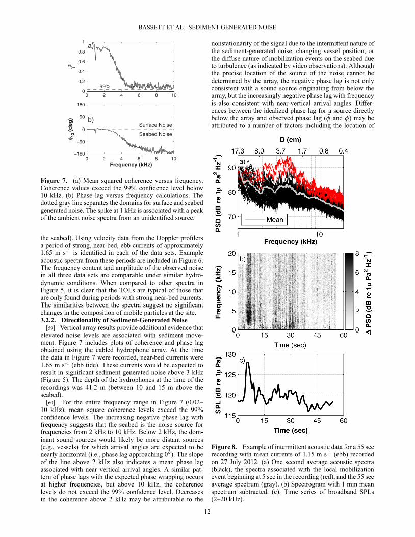
Figure 7. (a) Mean squared coherence versus frequency.Coherence values exceed the 99% confidence level below10 kHz. (b) Phase lag versus frequency calculations. Thedotted gray line separates the domains for surface and seabedgenerated noise. The spike at 1 kHz is associated with a peakof the ambient noise spectra from an unidentified source.

the seabed). Using velocity data from the Doppler profilersa period of strong, near-bed, ebb currents of approximately1.65 m s–1 is identified in each of the data sets. Exampleacoustic spectra from these periods are included in Figure 6.The frequency content and amplitude of the observed noisein all three data sets are comparable under similar hydro-dynamic conditions. When compared to other spectra inFigure 5, it is clear that the TOLs are typical of those thatare only found during periods with strong near-bed currents.The similarities between the spectra suggest no significantchanges in the composition of mobile particles at the site.3.2.2. Directionality of Sediment-Generated Noise

[59] Vertical array results provide additional evidence thatelevated noise levels are associated with sediment move-ment. Figure 7 includes plots of coherence and phase lagobtained using the cabled hydrophone array. At the timethe data in Figure 7 were recorded, near-bed currents were1.65 m s–1 (ebb tide). These currents would be expected toresult in significant sediment-generated noise above 3 kHz(Figure 5). The depth of the hydrophones at the time of therecordings was 41.2 m (between 10 and 15 m above theseabed).

[60] For the entire frequency range in Figure 7 (0.02–10 kHz), mean square coherence levels exceed the 99%confidence levels. The increasing negative phase lag withfrequency suggests that the seabed is the noise source forfrequencies from 2 kHz to 10 kHz. Below 2 kHz, the dom-inant sound sources would likely be more distant sources(e.g., vessels) for which arrival angles are expected to benearly horizontal (i.e., phase lag approaching 0ı). The slopeof the line above 2 kHz also indicates a mean phase lagassociated with near vertical arrival angles. A similar pat-tern of phase lags with the expected phase wrapping occursat higher frequencies, but above 10 kHz, the coherencelevels do not exceed the 99% confidence level. Decreasesin the coherence above 2 kHz may be attributable to the

nonstationarity of the signal due to the intermittent nature ofthe sediment-generated noise, changing vessel position, orthe diffuse nature of mobilization events on the seabed dueto turbulence (as indicated by video observations). Althoughthe precise location of the source of the noise cannot bedetermined by the array, the negative phase lag is not onlyconsistent with a sound source originating from below thearray, but the increasingly negative phase lag with frequencyis also consistent with near-vertical arrival angles. Differ-ences between the idealized phase lag for a source directlybelow the array and observed phase lag ( Q and ) may beattributed to a number of factors including the location of

Figure 8. Example of intermittent acoustic data for a 55 secrecording with mean currents of 1.15 m s–1 (ebb) recordedon 27 July 2012. (a) One second average acoustic spectra(black), the spectra associated with the local mobilizationevent beginning at 5 sec in the recording (red), and the 55 secaverage spectrum (gray). (b) Spectrogram with 1 min meanspectrum subtracted. (c). Time series of broadband SPLs(2–20 kHz).

12


1 sec. 5 sec.10 sec 30 sec.

0

0.25

0.5

0.75P

DF

4 kHz

0

0.25

0.5

0.75

PD

F

8 kHz

−8 −4 0 4 80

0.25

0.5

0.75

PD

F

Δ TOL (dB)

16 kHz

Figure 9. Probability distribution functions of the differ-ence between 55 sec TOLs and 1, 5, 10, and 30 sec TOLsfor ebb currents between 1.15 and 1.35 m s–1. Other veloc-ity bins and frequency bins are not shown but have similardistributions.

the noise sources on the seabed and off-vertical hydrophoneorientation. Although there was no significant wire angleobserved during the deployment, it is possible that verti-cal shear lower in the water column may have resultedin a horizontal displacement between the upper and lowerhydrophones changing the vertical separation distance andthe orientation angle of the line array resulting in a decreasedphase lag.3.2.3. Intermittency and Stationarity

[61] The sound produced by sediment grains shifting onthe seabed is not continuous. That is, bed load transport is

not sustained at a given location throughout the tidal cycle.The mean spectra are representative of characteristic noiselevels integrated over an area of the seabed under differenthydrodynamic conditions, but do not provide details abouttransient events. For example, a series of 1 sec averagespectra, a spectrogram with the 55 sec mean spectrum sub-tracted, and a time-series of broadband (2–20 kHz) soundpressure levels, presented in Figure 8, show the dominantsignal associated with a single local mobilization event.The peak intensities suggest that both the pebbles andgravel were mobilized. Manual review of the recorded audioreveals elevated noise levels attributable to sediment motionalthough the identification of individual events is generallynot possible (i.e., the spectra in Figure 8 are representa-tive of a minority of recordings when sediment generatednoise is present). However, when localized events occur nearthe hydrophone, the identification of sound from individualevents is possible. During these instances, the sound is sim-ilar to what one hears when gravel is poured over a pileof gravel. During these events, broadband sound pressurelevels increase by up to 15 dB with energy contained infrequency bands between 1 and 30 kHz.

[62] As demonstrated in Figure 8, intermittent signalsassociated with highly localized mobilization events havethe potential to impact sediment-generated noise statisticsbased on the averaging period or the duty cycle of the record-ing instrument. Figure 9 includes the probability distributionfunctions of the difference between TOLs calculated using55 sec averages and those calculated using 1, 5, 10, and30 sec averages for three frequencies (4, 8, and 16 kHz).For each frequency, the mean TOL is approximately thesame (< 1 dB difference) regardless of the length of therecording. However, as is expected for a weakly stationarysignal, in each case, the distribution is narrower for longeraveraging periods.

3.3. Noise Level Regressions[63] Regression statistics for the sound intensity versus

near-bed hydrodynamic power per unit area are included inTable 3 for the velocity bin averaged acoustic data and for

Table 3. Results and Statistics for the Noise Versus Velocity-Cubed Regressionsa

Ebb Flood

fc (kHz) am bm ucr (m s–1) R2 Time Series n R2 Bin Ave. am bm ucr (m s–1) R2 Time Series n R2 Bin Ave.

1 –85.4 0.0024 1.25 0.15 463 0.97 –87.6 0.0042 1.25 0.23 438 0.931.25 –85.1 0.0031 1.25 0.25 463 0.99 –88.4 0.0048 1.25 0.32 438 0.941.600 –83.5 0.0042 1.25 0.39 463 0.99 –87.7 0.0055 1.25 0.38 438 0.952.000 –83.6 0.0046 1.25 0.44 463 0.98 –87.9 0.0056 1.25 0.42 438 0.942.500 –86.1 0.0052 1.25 0.54 463 0.99 –89.3 0.0054 1.25 0.45 438 0.923.150 –86.1 0.0058 1.25 0.62 463 0.99 –89.9 0.0064 1.25 0.46 438 0.934.000 –84.5 0.0060 1.25 0.62 463 0.99 –88.0 0.0068 1.25 0.42 438 0.915.000 –84.9 0.0064 1.15 0.60 564 0.99 –86.6 0.0065 1.15 0.47 645 0.936.300 –86.6 0.0069 1.05 0.65 700 0.99 –88.9 0.0074 0.95 0.59 1049 0.968.000 –87.7 0.0075 0.95 0.67 782 0.98 –90.4 0.0082 0.85 0.70 1256 0.9810.000 –88.2 0.0078 0.85 0.68 837 0.98 –91.1 0.0089 0.85 0.73 1256 0.9812.500 –88.1 0.0076 0.85 0.62 837 0.98 –91.0 0.0091 0.85 0.70 1256 0.9816.000 –88.1 0.0075 0.85 0.55 837 0.97 –90.8 0.0090 0.85 0.67 1256 0.9820.000 –87.8 0.0069 0.85 0.52 837 0.97 –91.0 0.0088 0.85 0.67 1256 0.9825.000 –91.6 0.0078 0.65 0.59 949 0.96 –95.2 0.0102 0.85 0.72 1256 0.97

aCoefficients am (ambient noise) and bm (efficiency) correspond respectively to the y-intercept and slope of the acoustic intensity versus hydrodynamicpower for one-third octave bands. R2 values are calculated for the time series data with no vessels present using the coefficients from the velocity binaveraged regressions. The total number of points used to calculate raw R2 values is n. The threshold for significant noise increases, +3 dB from mean slacktide conditions is ucr(m s–1).

13


Figure 10. Comparison of observed noise levels and atime series constructed from the regressions coefficients for17 February 2011. Periods with currents exceeding 1 ms–1 are highlighted. (a) Measured spectrogram. The regularincreases in broadband noise levels during weak currents area result of vessel traffic. (b) Spectrogram reconstructed usingregression coefficients. (c) Near-bed currents.

the time series data using the regression coefficients obtainedfrom the bin averaged data (note again that the bin averageddata are required to identify critical near-bed velocities).The regression coefficients suggest that, in the absence ofsediment-generated noise, these frequency bands would berelatively quiet and that the conversion of hydrodynamicto acoustic power is inefficient. These are both physicallyrealistic relations and consistent with the prior discussion.For bin-averaged data, the R2 values for both flood and ebbcurrents exceed 0.9 for all frequency bands.

[64] The R2 values for the unbinned time series data arelowest at the low frequencies, but still highly significantgiven the total number of data points included in the regres-sions. The source of the lower R2 values, specifically atlower frequencies, can be explained by the low signal-to-noise ratio of sediment-generated noise to other ambientnoise sources and the section on intermittency and station-arity (section 3.2.3). Especially below 4 kHz, noise levelsduring periods of strong currents fall within the range asso-ciated with quiescent conditions. As such, scatter in the dataat these frequencies may be in part attributed to other noisesources. In all frequency bands, there is also more scatter inthe acoustic data during low currents.

[65] Based on the method, the onset of noise levelincreases is correlated with bed stresses on the order of3 Pa. In general, the regression slope coefficient increaseswith frequency, suggesting that hydrodynamic power ismore efficiently converted to acoustic power for small grainsizes. Just as mean shear stresses in a velocity bin varybetween flood and ebb currents, noise levels and the effi-ciencies also vary between flood and ebb tides. The ebb effi-ciencies, converted to an approximate noise level increasein 0.1 m s–1 bins, range from approximately 0.9 (1 kHz)to 3 dB (25 kHz) per 0.1 m s–1 increase in the near-bedvelocity. During flood tides, the comparable coefficients are1.5 (1 kHz) to 3.6 dB (25 kHz) per 0.1 m s–1 increase in thenear-bed velocity.

[66] To provide a qualitative example of the predictivevalue of the regression coefficients, a time series of TOLsand currents is included in Figure 10 for a 24 h period. Bothregression coefficients are only applied to TOLs when themean currents exceed the critical velocity (Table 3). Ves-sel traffic, which is not represented using the regressions,regularly increases TOLs in all measured frequency bands(as previously discussed, the regression values are derivedfrom observations without vessel traffic). During strong cur-rents, there is good agreement in received levels across allfrequency bands included in the regressions. This agree-ment demonstrates that sediment-generated noise levels atthe sites are highly predictable from the near-bed velocity,once site-specific regression coefficients have been obtained.At this site, strong spatial gradients result in significantreductions in currents at scales on the order of 100s ofmeters [Palodichuk et al., 2013]. As a result, sediment-generated noise levels are expected to change at comparablelength scales.

4. Discussion[67] The results presented here demonstrate a rich rela-

tionship between hydrodynamics, the physics of incipientmotion and mobilization of heterogeneous, coarse-grainedbeds, and ambient noise in high-energy environments. Asdemonstrated in Figure 5, sediment-generated noise is a sig-nificant source of ambient noise at this location. The inten-sity and regularity of sediment-generated noise is dependenton hydrodynamic conditions and seabed composition. Ifconditions regularly mobilize the bed, sediment-generatednoise can contribute significantly to ambient noise over abroad frequency range related to the local composition ofthe seabed.

4.1. Bed Stress and Sediment Mobilization[68] The shear stresses at which increases in ambient

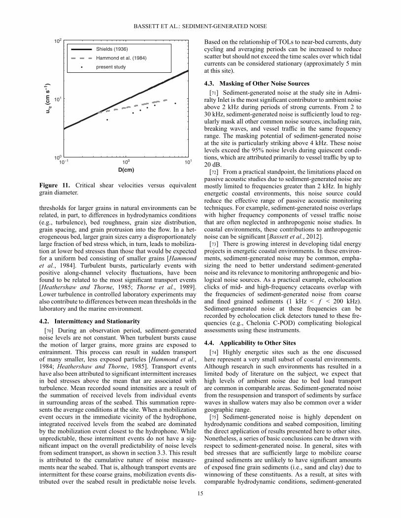
noise are attributed to sediment-generated noise are lowerthan previous estimates discussed in section 1. Again, wenote that the thresholds defined in this study are based onincreases in TOLs, which require regular mobilizations orcollisions between grains. In this study, noise levels forequivalent grains size up to 6 cm (f > 2.5 kHz) increasewith shear stresses greater than 7 Pa. By contrast, compara-ble values were noted by Thorne et al. [1989] for sand andgravel in a tidal channel and by Miller et al. [1977] for 1 cmequivalent grain sizes in experimental work. A comparisonbetween critical shear velocities (u�c) calculated for site spe-cific data, the Shield’s parameter (assuming ‚c = 0.06), andHammond et al. [1984] are included in Figure 11. The sitespecific critical shear stresses were calculated assuming adrag coefficient of 0.0044 (section 3.1) and the critical veloc-ity thresholds included in Table 3. The critical shear stressesfor all calculated grain sizes are lower than the critical valuesusing the Shields parameter and Hammond et al. [1984].

[69] The referenced thresholds for sediment movement,described in Miller et al. [1977], which covers literaturedating back to Shields [1936], are derived from simplifiedexperimental studies intended to reduce scatter in the datasets. Amongst the common design parameters are unidirec-tional flows, flumes with parallel sidewalls, and beds con-sisting of rounded, uniformly sized grains. Lower observed

14


Shields (1936)

Hammond et al. (1984)

present study

Figure 11. Critical shear velocities versus equivalentgrain diameter.

thresholds for larger grains in natural environments can berelated, in part, to differences in hydrodynamics conditions(e.g., turbulence), bed roughness, grain size distribution,grain spacing, and grain protrusion into the flow. In a het-erogeneous bed, larger grain sizes carry a disproportionatelylarge fraction of bed stress which, in turn, leads to mobiliza-tion at lower bed stresses than those that would be expectedfor a uniform bed consisting of smaller grains [Hammondet al., 1984]. Turbulent bursts, particularly events withpositive along-channel velocity fluctuations, have beenfound to be related to the most significant transport events[Heathershaw and Thorne, 1985; Thorne et al., 1989].Lower turbulence in controlled laboratory experiments mayalso contribute to differences between mean thresholds in thelaboratory and the marine environment.

4.2. Intermittency and Stationarity[70] During an observation period, sediment-generated

noise levels are not constant. When turbulent bursts causethe motion of larger grains, more grains are exposed toentrainment. This process can result in sudden transportof many smaller, less exposed particles [Hammond et al.,1984; Heathershaw and Thorne, 1985]. Transport eventshave also been attributed to significant intermittent increasesin bed stresses above the mean that are associated withturbulence. Mean recorded sound intensities are a result ofthe summation of received levels from individual eventsin surrounding areas of the seabed. This summation repre-sents the average conditions at the site. When a mobilizationevent occurs in the immediate vicinity of the hydrophone,integrated received levels from the seabed are dominatedby the mobilization event closest to the hydrophone. Whileunpredictable, these intermittent events do not have a sig-nificant impact on the overall predictability of noise levelsfrom sediment transport, as shown in section 3.3. This resultis attributed to the cumulative nature of noise measure-ments near the seabed. That is, although transport events areintermittent for these coarse grains, mobilization events dis-tributed over the seabed result in predictable noise levels.

Based on the relationship of TOLs to near-bed currents, dutycycling and averaging periods can be increased to reducescatter but should not exceed the time scales over which tidalcurrents can be considered stationary (approximately 5 minat this site).

4.3. Masking of Other Noise Sources[71] Sediment-generated noise at the study site in Admi-

ralty Inlet is the most significant contributor to ambient noiseabove 2 kHz during periods of strong currents. From 2 to30 kHz, sediment-generated noise is sufficiently loud to reg-ularly mask all other common noise sources, including rain,breaking waves, and vessel traffic in the same frequencyrange. The masking potential of sediment-generated noiseat the site is particularly striking above 4 kHz. These noiselevels exceed the 95% noise levels during quiescent condi-tions, which are attributed primarily to vessel traffic by up to20 dB.

[72] From a practical standpoint, the limitations placed onpassive acoustic studies due to sediment-generated noise aremostly limited to frequencies greater than 2 kHz. In highlyenergetic coastal environments, this noise source couldreduce the effective range of passive acoustic monitoringtechniques. For example, sediment-generated noise overlapswith higher frequency components of vessel traffic noisethat are often neglected in anthropogenic noise studies. Incoastal environments, these contributions to anthropogenicnoise can be significant [Bassett et al., 2012].

[73] There is growing interest in developing tidal energyprojects in energetic coastal environments. In these environ-ments, sediment-generated noise may be common, empha-sizing the need to better understand sediment-generatednoise and its relevance to monitoring anthropogenic and bio-logical noise sources. As a practical example, echolocationclicks of mid- and high-frequency cetaceans overlap withthe frequencies of sediment-generated noise from coarseand fined grained sediments (1 kHz < f < 200 kHz).Sediment-generated noise at these frequencies can berecorded by echolocation click detectors tuned to these fre-quencies (e.g., Chelonia C-POD) complicating biologicalassessments using these instruments.

4.4. Applicability to Other Sites[74] Highly energetic sites such as the one discussed

here represent a very small subset of coastal environments.Although research in such environments has resulted in alimited body of literature on the subject, we expect thathigh levels of ambient noise due to bed load transportare common in comparable areas. Sediment-generated noisefrom the resuspension and transport of sediments by surfacewaves in shallow waters may also be common over a widergeographic range.

[75] Sediment-generated noise is highly dependent onhydrodynamic conditions and seabed composition, limitingthe direct application of results presented here to other sites.Nonetheless, a series of basic conclusions can be drawn withrespect to sediment-generated noise. In general, sites withbed stresses that are sufficiently large to mobilize coarsegrained sediments are unlikely to have significant amountsof exposed fine grain sediments (i.e., sand and clay) due towinnowing of these constituents. As a result, at sites withcomparable hydrodynamic conditions, sediment-generated

15


noise is unlikely to be significant at high frequencies( f > 50 kHz, D � 0.1 cm, the upper limit for coarse sand)except in the cases of energetic estuaries with large sus-pended sediment loads from local inflows. More energeticsites are likely to produce noise at lower frequencies, unlessscoured to bedrock, because larger shear stresses can supportthe motion of larger grain sizes.

5. Conclusion[76] Analysis of hydrodynamic and acoustic measure-

ments from a site in Admiralty Inlet, Puget Sound, WA(USA) suggests that sediment-generated noise is the domi-nant noise source between 1 and 30 kHz during periods ofstrong currents. Peak sediment-generated noise levels from4 to 20 kHz are associated with mobile gravel and peb-bles. Sediment-generated noise levels in one-third octavebands exceed noise levels attributed to vessel noise byup to 20 dB. Equivalent grain sizes, estimated by invert-ing the acoustic spectra associated with sediment-generatednoise, are in agreement with the known distribution ofgrain sizes present at the site. Three methods of calculatingthe bed stress show good agreement for periods of strongcurrents. Using increases in noise levels at different fre-quencies, critical shear stresses for different grain sizes areestimated and found to be lower than laboratory studiesdespite the use of a more conservative definition of criti-cal shear stress. Regressions of the sound intensity versusthe near-bed hydrodynamic power per unit area show thatnoise levels are predictable and that the largest increasesin noise levels are associated with smaller grains (higherfrequencies). Localized, intermittent events can increaserecorded noise levels by more than 10 dB over a periodof seconds. Due to such events, the distribution of TOLsrecorded in a velocity bin is narrower for longer record-ing periods, as long as near-bed velocities can still beconsidered stationary.

[77] Acknowledgments. Thanks to field engineers Joe Talbert andAlex deKlerk for the successful recoveries and deployments of the tripods.Many thanks to Capt. Andy Reay-Ellers, the captain of the R/V JackRobertson, Andrea Ogston, Chris Chickadel, Sarah Giddings, and MichelleHickner. We also thank the three anonymous reviewers for their helpfulcomments on the manuscript. Snohomish Public Utility District’s inter-est in tidal energy was the motivation for studying ambient noise atthe site. Washington State Parks allowed for the placement of the AISsystem on Admiralty Head Lighthouse. Funding provided by U.S. Depart-ment of Energy award DE-EE0002654. Student support was provided toChristopher Bassett by National Science Foundation award DGE-0718124.

ReferencesBassett, C. (2010), Underwater ambient noise at a proposed tidal energy site

in Puget Sound, Master’s thesis, University of Washington.Bassett, C., B. Polagye, M. Holt, and J. Thomson (2012), A vessel noise

budget for Admiralty Inlet, Puget Sound, Washington (USA), J. Acoust.Soc. Am., 132(6), 3706–3719, doi:10.1121/1.4763548.

Brumley, B., R. Cabrera, K. Deines, and E. Terray (1991), Performance ofa broad-band acoustic doppler current profiler, IEEE J. Ocean. Eng.,16(4), 402–407, doi:10.1109/48.90905.

Diplas, P., C. Dancey, A. Celik, M. Valyrakis, K. Greer, and T. Akar(2008), The role of impulse on the initiation of particle movementunder turbulent flow conditions, Science, 322 (5902), 717–720, doi:10.1126/science.1158954.

Gobat, J. I., and M. Grosenbaugh (1997), Modeling the mechanical andflow-induced noise on the surface suspended acoustic receiver, 748–754,IEEE Oceans. doi:10.1109/OCEANS.1997.624086.

Goring, D., and V. Nikora (2002), Despiking acoustic doppler velocimeterdata, J. Hydraul. Eng., 128 (1), 117–126, doi:10.1061/(ASCE)0733-9429(2002)128:1(117).

Grant, W., A. Williams III, and S. Glenn (1984), Bottom stressestimates and their prediction on the Northern California con-tinental shelf during CODE-1: The importance of wave-currentinteraction, J. Phys. Oceanogr., 14 (3), 506–526, doi:10.1175/1520-0485(1984)014<0506:BSEATP>2.0.CO;2.

Green, M. (1992), Spectral estimates of bed shear stress at subcriticalreynolds numbers in a tidal boundary layer, J. Phys. Oceanogr., 22(8),903–917, doi:10.1175/1520-0485(1992)022<0903:SEOBSS>2.0.CO;2.

Greene, C. R., Jr., and S. Moore (1995), Man-made noise, in MarineMammals and Noise, pp. 101–158, Academic Press, San Diego.

Greene, H., (2011), Habitat characterization of the SnoPUD turbine site—Admiralty Head, Washington State, Tech. Rep., Sound and Sea Technol-ogy.

Gross, T., and A. Nowell (1983), Mean flow and turbulence scaling in a tidalboundary layer, Cont. Shelf Res., 2(2-3), 109–126, doi:10.1016/0278-4343(83)90011-0.

Hammond, F. D. C., A. D. Heathershaw, and D. N. Langhorne (1984), Acomparison between Shields’ threshold criterion and the movement ofloosely packed gravel in a tidal channel, Sedimentology, 31, 51–62, doi:10.1111/j.1365-3091.1984.tb00722.

Harden Jones, F., and R. Mitson (1982), The movement of noisy sand-waves in the Strait of Dover, ICES J. Mar. Sci., 40 (1), 53–61, doi:10.1093/icesjms/40.1.53.

Heathershaw, A. (1979), The turbulent structure of the bottom boundarylayer in a tidal channel, Geophys. J. R. Astron. Soc., 58, 395–430, doi:10.1111/j.1365-246X.1979.tb01032.X.

Heathershaw, A. D., and P. D. Thorne (1985), Sea-bed noises reveal role ofturbulent bursting phenomenon in sediment transport by tidal currents,Nature, 316(6026), 339–342, doi:10.1038/316339a0.

Lee, H., and S. Balachandar (2012), Critical shear stress for incipientmotion of a particle on a rough bed, J. Geophys. Res., 117(F01026), 1–19,doi:10.1029/2011JF002208.

Lu, Y., R. Lueck, and D. Huang (2000), Turbulence characteristics ina tidal channel, J. Phys. Oceanogr., 30, 855–867, doi:10.1175/1520-0485(2000)030<0855:TCIATC>2.0.CO;2.

Lueck, R., and Y. Lu (1997), The logarithmic layer in a tidal chan-nel, Cont. Shelf Res., 17(14), 1785–1801, doi:10.1016/S0278-4343(97)00049-6.

Ma, B., J. Nystuen, and R.-C. Lien (2005), Prediction of underwater soundlevels from rain and wind, J. Acoust. Soc. Am., 117(6), 3555–3565, doi:10.1121/1.1910283.

Mason, T., D. Priestley, and D. Reeve (2007), Monitoring near-shore shin-gle transport under waves using a passive acoustic technique, J. Acoust.Soc. Am., 122(2), 737–746, doi:10.1121/1.2747196.

Mellen, R. (1952), The thermal-noise limit in the detection of under-water acoustic signals, J. Acoust. Soc. Am., 24 (5), 478–480, doi:10.1121/1.1906924.

Miller, M., I. McCave, and P. Komar (1977), Threshold of sedimentmotion under unidirectional currents, Sedimentology, 24(4), 507–527,doi:10.1111/j.1365-3091.1977.tb00136.X.

Mori, N., T. Suzuki, and S. Kakuno (2007), Noise of acoustic Dopplervelocimeter data in bubbly flows, J. Eng. Mech., 133(1), 122–125, doi:10.1061/(ASCE)0733-9399(2007)133:1(122).

Nystuen, J., and H. Selsor (1997), Weather classification using pas-sive acoustic drifters, J. Atmos. Oceanic Technol., 14, 656–666, doi:10.1175/1520-0426(1997)014<0656:WCUPAD>2.0.CO;2 .

Polagye, B., and J. Thomson (2013), Tidal energy resourcecharacterization: Methodology and field study in Admiralty Inlet,Puget Sound, US, IMechE, Part A: J. Power and Energy, doi:10.1177/0957650912470081.

Polagye, B., B. Van Cleve, A. Copping, and K. Kirkendall, (2011), Envi-ronmental effects of tidal energy development, Tech. Rep., 186 p, U.S.Dept. Commerce, NOAA Tech. Memo. NMFS F/SPO-116.

Palodichuk, M., B. Polagye, and J. Thomson (2013), Resource mapping attidal energy sites, J. Ocean. Eng., doi:10.1109/JOE.2012.2227578.

Priestley, M. (1981), Spectral Analysis and Time Series, 467, 660–661,Academic Press, London.

Schwehr, K. (2010), Python software for processing ais data. v0.43.Shields, A. (1936), Application of similarity principles and turbulence

research to bedload movement, Translated from Anwendung derAchnichkeits Geschiebebewegung, in Mitt. Preuss. VersAnst. Wasserb.Schiftb., edited by W. D. Ott, and J. C. von Vcheten, vol. 167, 36 p.,Publ. Calif. Inst. Technol. Hydrodyn. Lab.

Snohomish PUD, (2012), Admiralty Inlet pilot tidal project, FERC projectno. 12690, Tech. Rep., Public Utility District No. 1 of Snohomish County.

Strasberg, M. (1984), Adaptive Methods in Underwater Acoustics,125–143, Reidel, Boston, MA.

Strasberg, M. (1988), Dimensional analysis of windscreen noise, J. Acoust.Soc. Am., 83(2), 544–548, doi:10.1121/1.396148.

16


Strasberg, N. (1979), Nonacoustic noise interference in measurements ofinfrasonic ambient noise, J. Acoust. Soc. Am., 66(5), 1487–1493, doi:10.1121/1.383543.

Tennekes, H. (1973), The logarithmic wind profile, J. Atmos. Sci., 30,234–238, doi:10.1175/1520-0469(1973)030<0234:TLWP>2.0.CO;2.

Thompson, R. O. (1979), Coherence significance levels, J. of Atmos. Sci.,36, 2020–2021, doi:10.1175/1520-0469(1979)036<2020:CSL>2.0.CO;2.

Thomson, J., B. Polagye, V. Durgesh, and M. Richmond (2012), Measure-ments of turbulence at two tidal energy sites in Puget Sound, WA (USA),IEEE J. Ocean. Eng., 37(3), 363–374, doi:10.1109/JOE.2012.2191656.

Thorne, P. (1985), The measurement of acoustic noise generated by mov-ing artificial sediments, J. Acoust. Soc. Am., 78 (3), 1013–1023, doi:10.1121/1.393018.

Thorne, P. (1986a), Laboratory and marine measurements on the acousticdetection of sediment transport, J. Acoust. Soc. Am., 80(3), 899–910, doi:10.1121/1.393913.

Thorne, P. (1986b), An intercomparison between visual and acousticdetection of seabed gravel movement, Mar. Geol., 72, 11–31, doi:10.1016/0025-3227(86)90096-4.

Thorne, P. D., J. J. Williams, and A. D. Heathershaw (1989), In situ acousticmeasurements of marine gravel threshold and transport, Sedimentology,36, 61–74, doi:10.1111/j.1365-3091.1989.tb00820.X.

Thorne, P. (1990), Seabed generation of ambient noise, J. Acoust. Soc. Am.,87(1), 149–153, doi:10.1121/1.399307.

Trowbridge, J., W. Geyer, M. Bowen, and A. Williams III (1999), Near-bottom turbulence measurements in a partially mixed estuary: Turbu-lent energy balance, velocity structure, and along-channel momentumbalance, J. Phys. Oceanogr., 29 (2), 3056–3072, doi:10.1175/1520-0485(1999)029<3056:NBTMIA>2.0.CO;2.

Voglis, G., and J. Cook (1970), A new source of acoustic noiseobserved in the North Sea, Ultrasonics, 8, 100–101, doi:10.1016/0041-624X(70)90049-1.

Wentworth, C. K. (1922), A scale of grade and class terms for clasticsediments, J. Geol., 30(5), 377–392.

Wenz, G. (1962), Acoustic ambient noise in the ocean: Spectra and sources,J. Acoust. Soc. Am., 34(12), 1936–1956, doi:10.1121/1.1909155.

Williams, J., P. Thorne, and A. Heathershaw (1989), Measurements of tur-bulence in the benthic boundary layer over a gravel bed, Sedimentology,36, 959–971, doi:10.1111/j.1365-3091.1989.tb01533.X.

17

sedimentgenerated noise and bed stress in a tidal...

Documents