section 6.5: partial fractions and logistic growth
DESCRIPTION
Section 6.5: Partial Fractions and Logistic Growth. These are called non-repeating linear factors. 1. This would be a lot easier if we could re-write it as two separate terms. You may already know a short-cut for this type of problem. We will get to that in a few minutes. 1. - PowerPoint PPT PresentationTRANSCRIPT

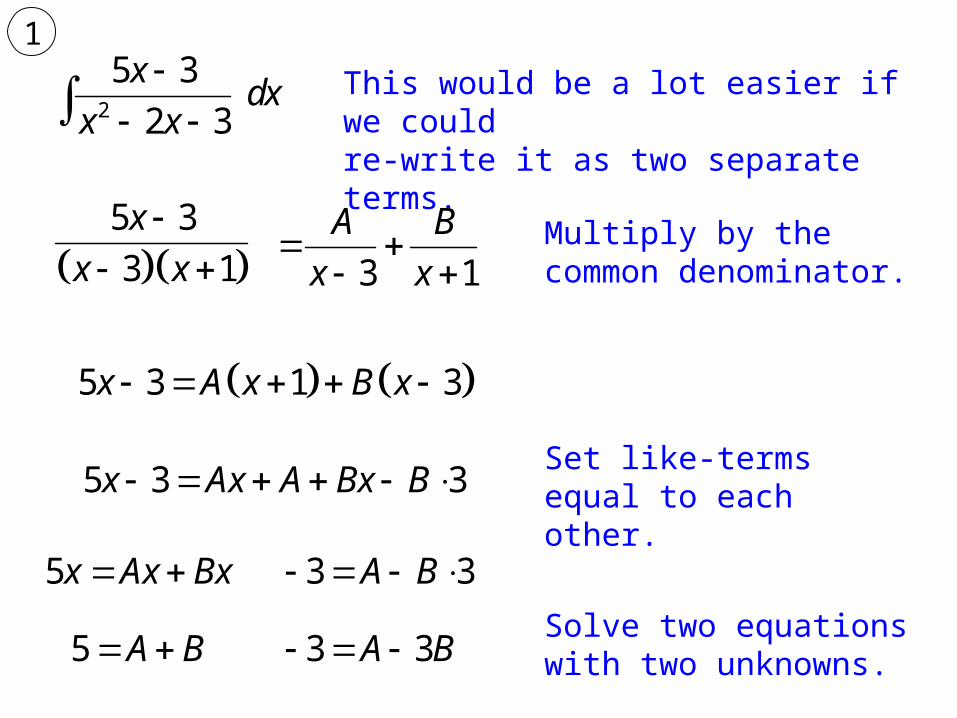
Section 6.5:Partial Fractions and Logistic Growth

2
5 3
2 3
xdx
x x
This would be a lot easier if we could
re-write it as two separate terms.
5 3
3 1
x
x x
3 1
A B
x x
1
These are called non-repeating linear factors.
You may already know a short-cut for this type of problem. We will get to that in a few minutes.
2
5 3
2 3
xdx
x x
This would be a lot easier if we could
re-write it as two separate terms.
5 3
3 1
x
x x
3 1
A B
x x
Multiply by the common denominator.
5 3 1 3x A x B x
5 3 3x Ax A Bx B Set like-terms equal to each other.
5x Ax Bx 3 3A B
5 A B 3 3A B Solve two equations with two unknowns.
1
2
5 3
2 3
xdx
x x
5 3
3 1
x
x x
3 1
A B
x x
5 3 1 3x A x B x
5 3 3x Ax A Bx B
5x Ax Bx 3 3A B
5 A B 3 3A B Solve two equations with two unknowns.
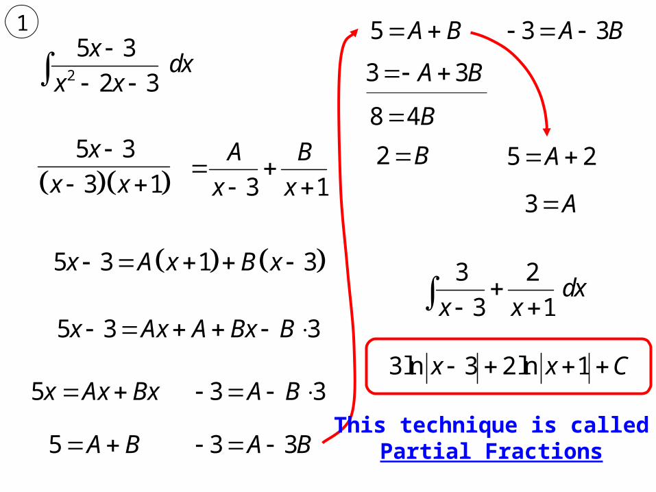
5 A B 3 3A B
3 3A B
8 4B
2 B 5 2A
3 A
3 2
3 1dx
x x
3ln 3 2ln 1x x C
This technique is calledPartial Fractions
1
2
5 3
2 3
xdx
x x
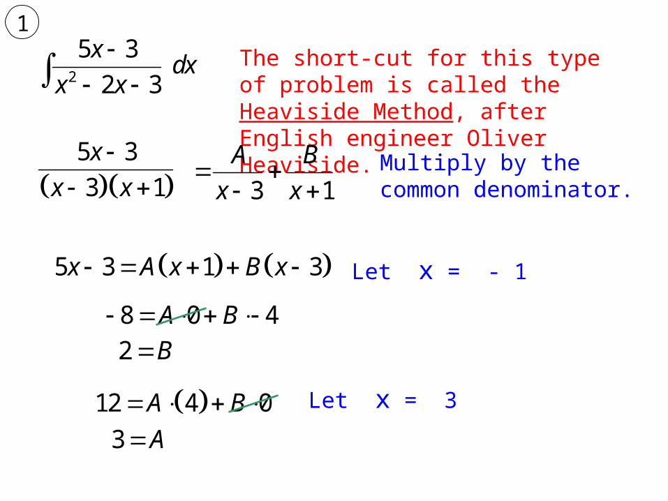
The short-cut for this type of problem is
called the Heaviside Method, after English engineer Oliver Heaviside.
5 3
3 1
x
x x
3 1
A B
x x
Multiply by the common denominator.
5 3 1 3x A x B x
8 0 4A B
1
Let x = - 1
2 B
12 4 0A B Let x = 3
3 A
2
5 3
2 3
xdx
x x
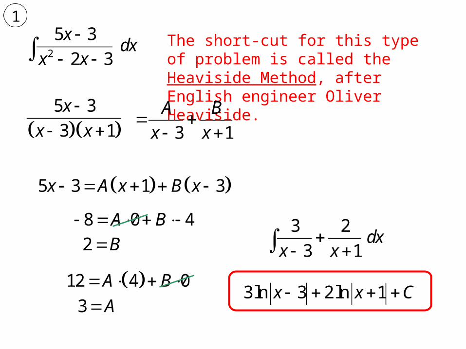
The short-cut for this type of problem is
called the Heaviside Method, after English engineer Oliver Heaviside.
5 3
3 1
x
x x
3 1
A B
x x
5 3 1 3x A x B x
8 0 4A B
1
2 B
12 4 0A B 3 A
3 2
3 1dx
x x
3ln 3 2ln 1x x C
3 2
2
2 4 3
2 3
x x x
x x
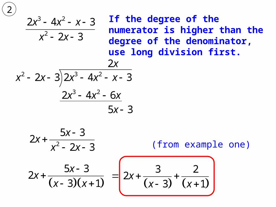
If the degree of the numerator is higher than the degree of the denominator, use long division first.
2 3 22 3 2 4 3x x x x x 2x
3 22 4 6x x x 5 3x
2
5 32
2 3
xxx x
5 3
23 1
xx
x x
3 2
23 1
xx x
2
(from example one)

We have used the exponential growth equationto represent population growth.
0kty y e
The exponential growth equation occurs when the rate of growth is proportional to the amount present.
If we use P to represent the population, the differential equation becomes: dP
kPdt
The constant k is called the relative growth rate.
/dP dtk
P
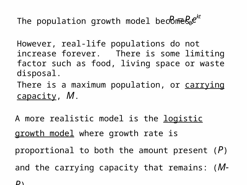
The population growth model becomes: 0ktP Pe
However, real-life populations do not increase forever. There is some limiting factor such as food, living space or waste disposal.
There is a maximum population, or carrying capacity, M.
A more realistic model is the logistic growth model where
growth rate is proportional to both the amount present (P)
and the carrying capacity that remains: (M-P)
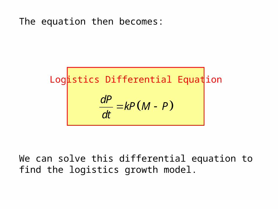
The equation then becomes:
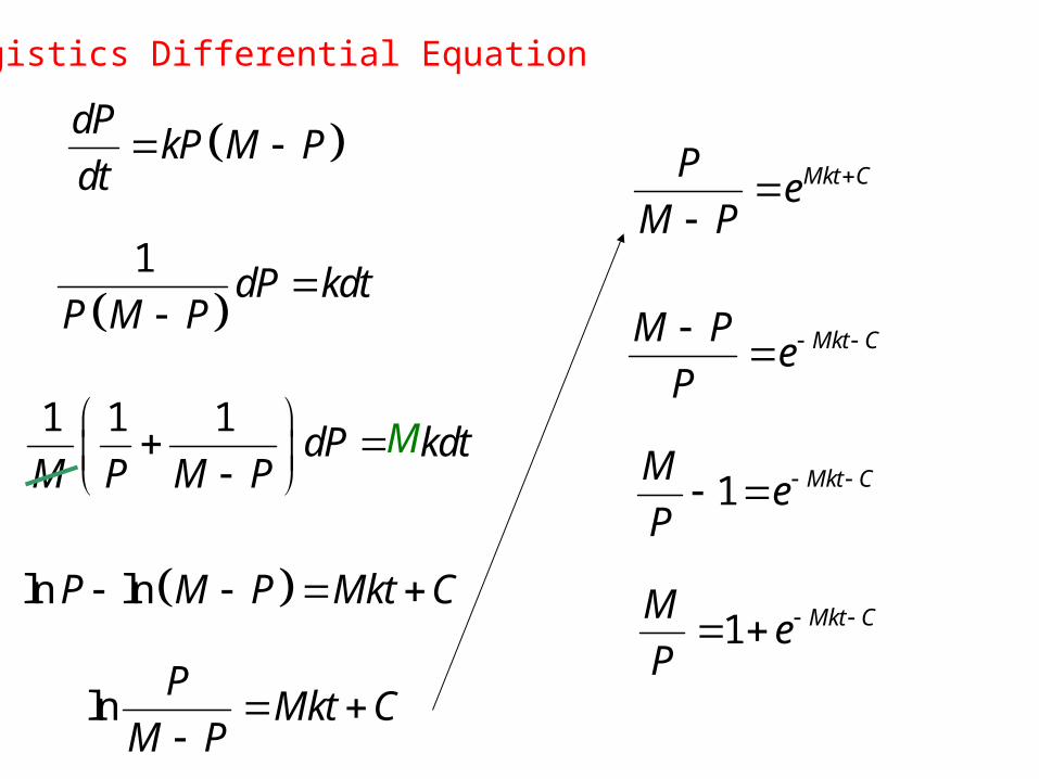
Logistics Differential Equation
dPkP M P
dt
We can solve this differential equation to find the logistics growth model.
PartialFractions
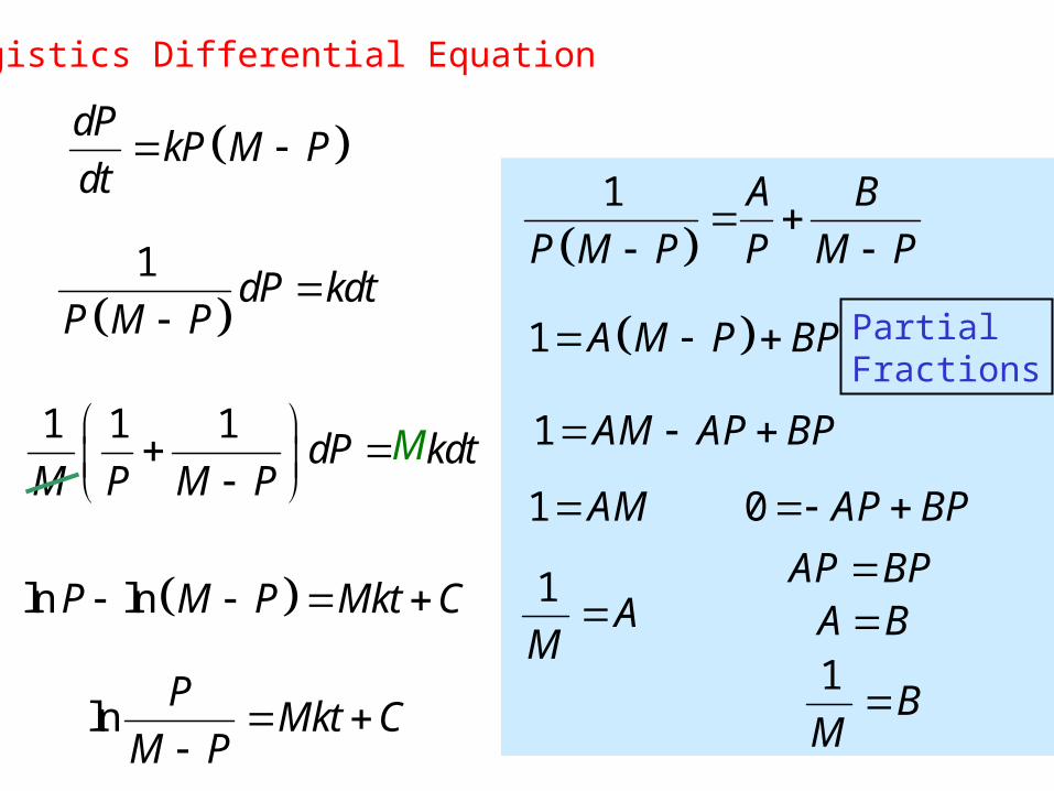
Logistics Differential Equation
dPkP M P
dt
1
dP kdtP M P
1 A B
P M P P M P
1 A M P BP
1 AM AP BP
1 AM
1A
M
0 AP BP AP BPA B1
BM
1 1 1 dP kdt
M P M P
ln lnP M P Mkt C
lnP
Mkt CM P
M
Logistics Differential Equation
Mkt CPe
M P
Mkt CM Pe
P
1 Mkt CMe
P
1 Mkt CMe
P
dPkP M P
dt
1
dP kdtP M P
1 1 1 dP kdt
M P M P
ln lnP M P Mkt C
lnP
Mkt CM P
M
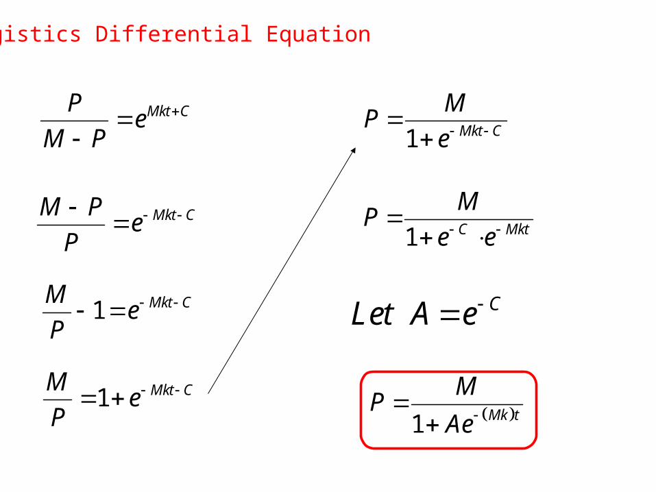
Logistics Differential Equation
1 Mkt C
MP
e
1 C Mkt
MP
e e
CLet A e
1 Mk t
MP
Ae
Mkt CPe
M P
Mkt CM Pe
P
1 Mkt CMe
P
1 Mkt CMe
P
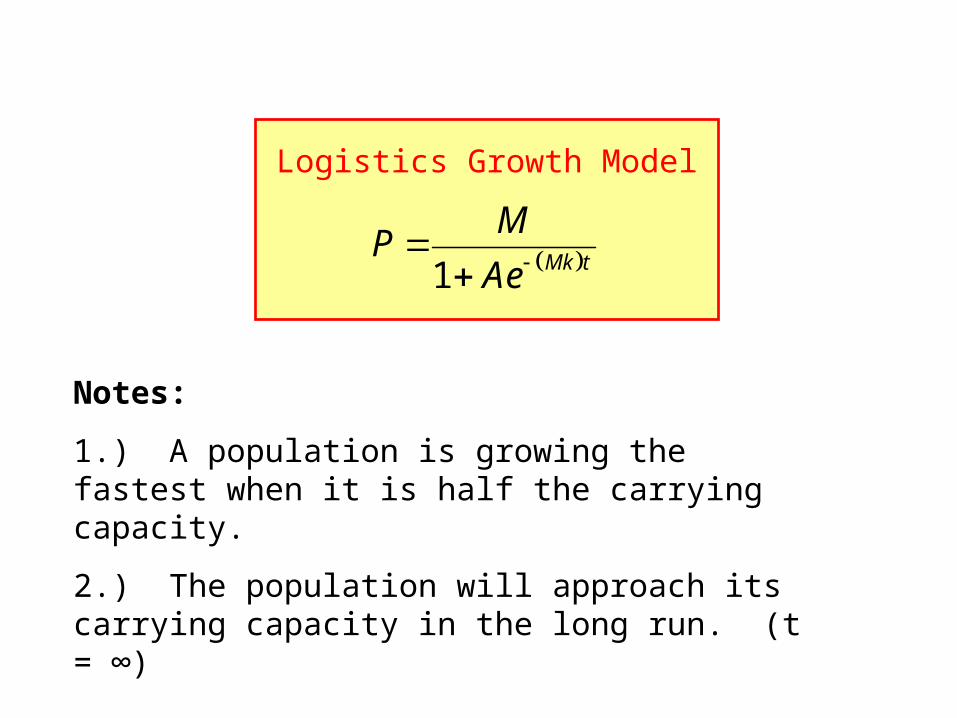
Logistics Growth Model
1 Mk t
MP
Ae
Notes:
1.) A population is growing the fastest when it is half the carrying capacity.
2.) The population will approach its carrying capacity in the long run. (t = ∞)
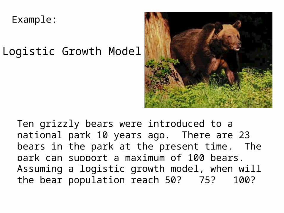
Example:
Logistic Growth Model
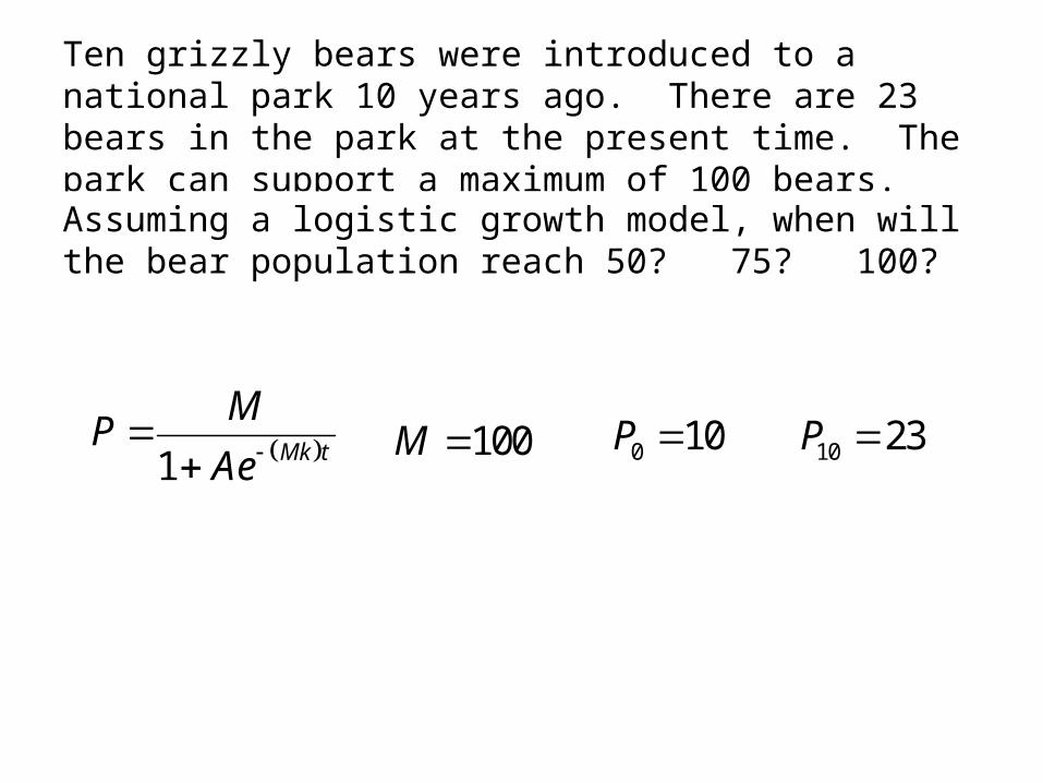
Ten grizzly bears were introduced to a national park 10 years ago. There are 23 bears in the park at the present time. The park can support a maximum of 100 bears.
Assuming a logistic growth model, when will the bear population reach 50? 75? 100?
Ten grizzly bears were introduced to a national park 10 years ago. There are 23 bears in the park at the present time. The park can support a maximum of 100 bears.
Assuming a logistic growth model, when will the bear population reach 50? 75? 100?
1 Mk t
MP
Ae
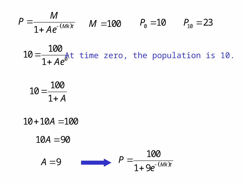
100M 0 10P 10 23P
1 Mk t
MP
Ae
100M 0 10P 10 23P
0
10010
1 Ae
10010
1 A
10 10 100A
10 90A
9A
At time zero, the population is 10.
100
1 9 Mk tP
e
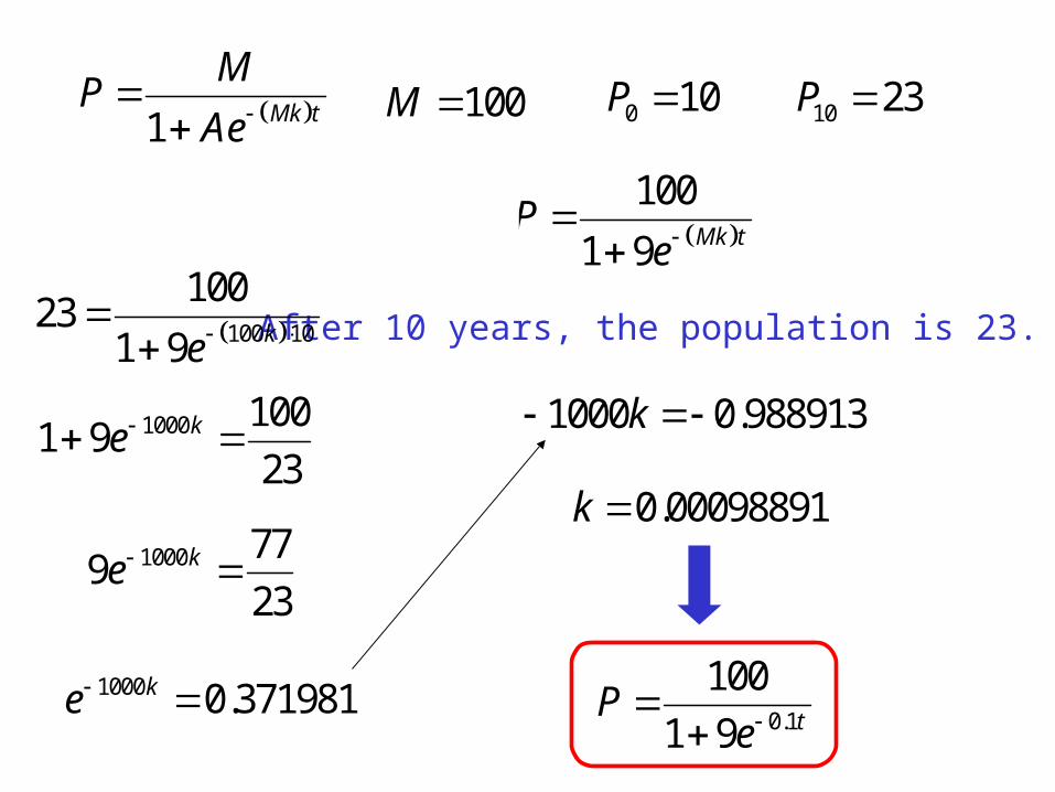
100M 0 10P 10 23P
After 10 years, the population is 23.
100
1 9 Mk tP
e
100 10
10023
1 9 ke
1000 1001 9
23ke
1000 779
23ke
1000 0.371981ke
1000 0.988913k
0.00098891k
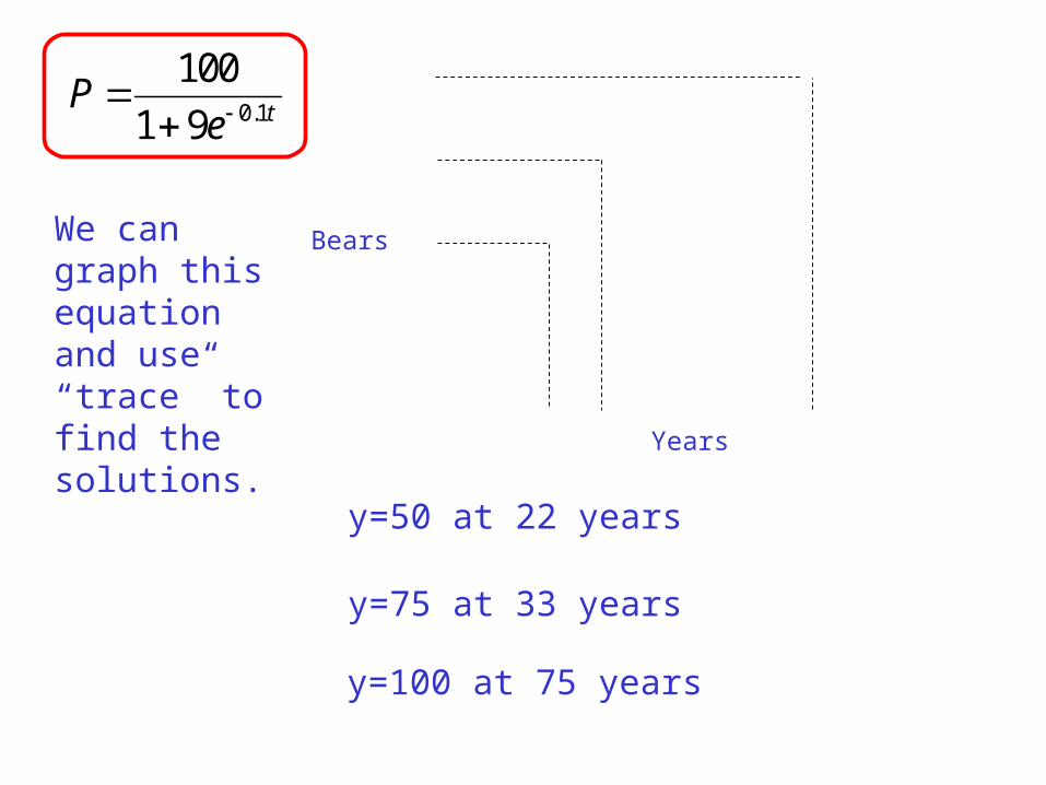
0.1
100
1 9 tP
e
1 Mk t
MP
Ae
0.1
100
1 9 tP
e
Years
BearsWe can graph this equation and use “trace” to find the solutions.
y=50 at 22 years
y=75 at 33 years
y=100 at 75 years